phisx: quantum physics - tu clausthalorion.pt.tu-clausthal.de/atp/downloads/scripts/qm.pdf ·...
TRANSCRIPT
don’t p
anic!
Theoretical Physics IIIQuantum Theory
Peter E. Blöchl
Caution! This version is not completed and may containerrors
Institute of Theoretical Physics; Clausthal University of Technology;D-38678 Clausthal Zellerfeld; Germany;http://www.pt.tu-clausthal.de/atp/
2
© Peter Blöchl, 2000-August 4, 2019Source: http://www2.pt.tu-clausthal.de/atp/phisx.html
Permission to make digital or hard copies of this work or portions thereof for personal or classroomuse is granted provided that copies are not made or distributed for profit or commercial advantage andthat copies bear this notice and the full citation. To copy otherwise requires prior specific permissionby the author.
1
1To the title page: What is the meaning of ΦSX? Firstly, it sounds like “Physics”. Secondly, the symbols stand forthe three main pillars of theoretical physics: “X” is the symbol for the coordinate of a particle and represents ClassicalMechanics. “Φ” is the symbol for the wave function and represents Quantum Mechanics and “S” is the symbol for theEntropy and represents Statistical Physics.

Foreword and Outlook
At the beginning of the 20th century physics was shaken by two big revolutions. One was the theoryof relativity, the other was quantum theory. The theory of relativity introduces a large but finiteparameter, the speed of light. The consequence is a unified description of space and time. Quantumtheory introduces a small but finite parameter, the Planck constant. The consequence of quantumtheory is a unified concept of particles and waves.
Quantum theory describes the behavior of small things. Small things behave radically differentthan what we know from big things. Quantum theory becomes unavoidable to describe nature atsmall dimensions. Not only that, but the implications of quantum mechanics determine also how ourmacroscopic world looks like. For example, in a purely classical world all matter would essentiallycollapse into a point, leaving a lot of light around.
Quantum mechanics is often considered difficult. It seems counterintuitive, because the pictureof the world provided in classical physics, which we have taken for granted, is inaccurate. Our mindnaturally goes into opposition, if observations conflict with the well proven views we make of ourworld and which work so successfully for our everyday experiences. Teaching, and learning, quantummechanics is therefore a considerable challenge. It is also one of the most exciting tasks, becauseit enters some fundamentally new aspects into our thinking. In contrast to many quotes, it is mystrong belief that one can “understand” quantum mechanics just as one can “understand” classicalmechanics2. However, on the way, we have to let go of a number of prejudices that root deep in ourmind.
Because quantum mechanics appears counterintuitive and even incomplete due to its probabilisticelements, a number of different interpretations of quantum mechanics have been developed. Theycorrespond to different mathematical representations of the same theory. I have chosen to startwith a description using fields which is due to Erwin Schrödinger, because I can borrow a number ofimportant concepts from the classical theory of electromagnetic radiation. The remaining mysteryof quantum mechanics is to introduce the particle concept into a field theory. However, otherformulations will be introduced later in the course.
I have structured the lecture in the following way:In the first part, I will start from the experimental observations that contradict the so-called
classical description of matter.I will then try to sketch how a theory can be constructed that captures those observations. I
will not start from postulates, as it is often done, but demonstrate the process of constructing thetheory. I find this process most exciting, because it is what a scientist has to do whenever he is facedwith a new experimental facts that do not fit into an existing theory. Quantum mechanics comes intwo stages, called first and second quantization. In order to understand what quantum mechanicsis about, both stages are required, even though the second part is considered difficult and is oftentaught in a separate course. I will right from the beginning describe what both stages are about, inorder to clear up the concepts and in order to put the material into a proper context. However, inorder to keep the project tractable, I will demonstrate the concepts on a very simple, but specific
2This philosophical question requires however some deep thinking about what understanding means. Often theproblems understanding quantum mechanics are rooted in misunderstandings about what it means to understandclassical mechanics.
3

4
example and sacrifice mathematical rigor and generality. This is, however, not a course on secondquantization, and after the introduction, I will restrict the material to the first quantization until Icome to the last chapter.
Once the basic elements of the theory have been developed, I will demonstrate the consequenceson some one-dimensional examples. Then it is time to prepare a rigorous mathematical formu-lation. I will discuss symmetry in some detail. In order to solve real world problems it is importantto become familiar with the most common approximation techniques. Now we are prepared to ap-proach physical problems such as atoms and molecules. Finally we will close the circle by discussingrelativistic particles and many particle problems.
There are a number of textbooks available. The following citations3 are not necessarily completeor refer to the most recent edition. Nevertheless, the information should allow to locate the mostrecent version of the book.
• Cohen-Tannoudji, Quantenmechanik[3]. In my opinion a very good and modern textbook withlots of interesting extensions.
• Schiff, Quantum Mechanics[1]. Classical textbook.
• Gasiorowicz, Quantenphysik[2].
• Merzbacher, Quantum mechanics[3].
• Alonso and Finn, Quantenphysik[1],
• Atkins, Molecular Quantum Mechanics[4]. This book is a introductory text on quantum me-chanics with focuses on applications to molecules and descriptions of spectroscopic techniques.
• Messiah, Quantum Mechanics[2]. A very good older text with extended explanations. Veryuseful are the mathematical appendices.
• W. Nolting, Grundkurs Theoretische Physik 5: Quantenmechanik [4]. Compact and detailedtext with a lot of problems and solutions.
• C. Kiefer Quantentheorie [5] Not a text book but easy reading for relaxation. [6]J.-L. Basdevantand J. Dalibard, Quantum mechanics. A very good course book from the Ecole Polytechnique,which links theory well upon modern themes. It is very recent (2002).
3Detailed citations are compiled at the end of this booklet.

Contents
1 Waves? Particles? Particle waves! 13
2 Experiment: the double slit 152.1 Macroscopic particles: playing golf . . . . . . . . . . . . . . . . . . . . . . . . . . . 152.2 Macroscopic waves: water waves . . . . . . . . . . . . . . . . . . . . . . . . . . . . 162.3 Microscopic waves: light . . . . . . . . . . . . . . . . . . . . . . . . . . . . . . . . 212.4 Microscopic particles: electrons . . . . . . . . . . . . . . . . . . . . . . . . . . . . . 222.5 Summary . . . . . . . . . . . . . . . . . . . . . . . . . . . . . . . . . . . . . . . . 232.6 Recommended exercises . . . . . . . . . . . . . . . . . . . . . . . . . . . . . . . . 23
3 Towards a theory 253.1 Particles: classical mechanics revisited . . . . . . . . . . . . . . . . . . . . . . . . . 25
3.1.1 Hamilton formalism . . . . . . . . . . . . . . . . . . . . . . . . . . . . . . . 273.2 Waves: the classical linear chain . . . . . . . . . . . . . . . . . . . . . . . . . . . . 29
3.2.1 Equations of motion ... . . . . . . . . . . . . . . . . . . . . . . . . . . . . . 293.2.2 ... and their solutions . . . . . . . . . . . . . . . . . . . . . . . . . . . . . . 30
3.3 Continuum limit: transition to a field theory . . . . . . . . . . . . . . . . . . . . . . 323.4 Differential operators, wave packets, and dispersion relations . . . . . . . . . . . . . 333.5 Breaking translational symmetry . . . . . . . . . . . . . . . . . . . . . . . . . . . . 353.6 Introducing mass into the linear chain (Home study) . . . . . . . . . . . . . . . . . 393.7 Measurements . . . . . . . . . . . . . . . . . . . . . . . . . . . . . . . . . . . . . . 413.8 Postulates of Quantum mechanics . . . . . . . . . . . . . . . . . . . . . . . . . . . 433.9 Is Quantum theory a complete theory? . . . . . . . . . . . . . . . . . . . . . . . . . 443.10 Planck constant . . . . . . . . . . . . . . . . . . . . . . . . . . . . . . . . . . . . . 453.11 Wavy waves are chunky waves: second quantization . . . . . . . . . . . . . . . . . . 453.12 Summary . . . . . . . . . . . . . . . . . . . . . . . . . . . . . . . . . . . . . . . . 46
4 Quantum effects 474.1 Quasi-one-dimensional problems in the real world . . . . . . . . . . . . . . . . . . . 484.2 Time-independent Schrödinger equation . . . . . . . . . . . . . . . . . . . . . . . . 504.3 Method of separation of variables . . . . . . . . . . . . . . . . . . . . . . . . . . . 514.4 Free particles and spreading wave packets . . . . . . . . . . . . . . . . . . . . . . . 54
4.4.1 Wave packets delocalize with time . . . . . . . . . . . . . . . . . . . . . . . 554.4.2 Wick rotation . . . . . . . . . . . . . . . . . . . . . . . . . . . . . . . . . . 574.4.3 Galilei invariance (home study) . . . . . . . . . . . . . . . . . . . . . . . . . 57
4.5 Particle in a box, quantized energies and zero-point motion . . . . . . . . . . . . . . 58
5

6 CONTENTS
4.5.1 Time-dependent solutions for the particle in the box . . . . . . . . . . . . . 624.6 Potential step and splitting of wave packets . . . . . . . . . . . . . . . . . . . . . . 65
4.6.1 Kinetic energy larger than the potential step . . . . . . . . . . . . . . . . . 654.6.2 Construct the other partial solution using symmetry transformations . . . . . 674.6.3 Kinetic energy smaller than the potential step . . . . . . . . . . . . . . . . . 724.6.4 Logarithmic derivative . . . . . . . . . . . . . . . . . . . . . . . . . . . . . 73
4.7 Barrier and tunnel effect . . . . . . . . . . . . . . . . . . . . . . . . . . . . . . . . 744.8 Particle in a well and resonances . . . . . . . . . . . . . . . . . . . . . . . . . . . . 774.9 Summary . . . . . . . . . . . . . . . . . . . . . . . . . . . . . . . . . . . . . . . . 794.10 Recommended exercises . . . . . . . . . . . . . . . . . . . . . . . . . . . . . . . . 80
5 Language of quantum mechanics 815.1 Kets and the linear space of states . . . . . . . . . . . . . . . . . . . . . . . . . . . 81
5.1.1 Axioms . . . . . . . . . . . . . . . . . . . . . . . . . . . . . . . . . . . . . 835.1.2 Bra’s and brackets . . . . . . . . . . . . . . . . . . . . . . . . . . . . . . . 855.1.3 Some vocabulary . . . . . . . . . . . . . . . . . . . . . . . . . . . . . . . . 85
5.2 Operators . . . . . . . . . . . . . . . . . . . . . . . . . . . . . . . . . . . . . . . . 855.2.1 Axioms . . . . . . . . . . . . . . . . . . . . . . . . . . . . . . . . . . . . . 865.2.2 Some vocabulary . . . . . . . . . . . . . . . . . . . . . . . . . . . . . . . . 87
5.3 Analogy between states and vectors . . . . . . . . . . . . . . . . . . . . . . . . . . 915.4 The power of the Dirac notation . . . . . . . . . . . . . . . . . . . . . . . . . . . . 925.5 Extended Hilbert space . . . . . . . . . . . . . . . . . . . . . . . . . . . . . . . . . 925.6 Application: harmonic oscillator . . . . . . . . . . . . . . . . . . . . . . . . . . . . 92
5.6.1 Algebraic treatment of the one-dimensional harmonic oscillator . . . . . . . 935.6.2 Wave functions of the harmonic oscillator . . . . . . . . . . . . . . . . . . . 965.6.3 Multidimensional harmonic oscillator . . . . . . . . . . . . . . . . . . . . . . 97
6 Representations 1016.1 Unity operator . . . . . . . . . . . . . . . . . . . . . . . . . . . . . . . . . . . . . . 1016.2 Representation of a state . . . . . . . . . . . . . . . . . . . . . . . . . . . . . . . . 1026.3 Representation of an operator . . . . . . . . . . . . . . . . . . . . . . . . . . . . . 1036.4 Change of representations . . . . . . . . . . . . . . . . . . . . . . . . . . . . . . . 1036.5 From bra’s and ket’s to wave functions . . . . . . . . . . . . . . . . . . . . . . . . 104
6.5.1 Real-space representation . . . . . . . . . . . . . . . . . . . . . . . . . . . 1046.5.2 Momentum representation . . . . . . . . . . . . . . . . . . . . . . . . . . . 1066.5.3 Orthonormality condition of momentum eigenstates (Home study) . . . . . 107
6.6 Application: Two-state system . . . . . . . . . . . . . . . . . . . . . . . . . . . . . 1086.6.1 Pauli Matrices . . . . . . . . . . . . . . . . . . . . . . . . . . . . . . . . . . 1106.6.2 Excursion: The Fermionic harmonic oscillator (Home study) . . . . . . . . . 111
7 Measurements 1137.1 Expectation values . . . . . . . . . . . . . . . . . . . . . . . . . . . . . . . . . . . 1137.2 Certain measurements . . . . . . . . . . . . . . . . . . . . . . . . . . . . . . . . . 113
7.2.1 Schwarz’ inequality . . . . . . . . . . . . . . . . . . . . . . . . . . . . . . . 1157.3 Eigenstates . . . . . . . . . . . . . . . . . . . . . . . . . . . . . . . . . . . . . . . 1167.4 Heisenberg’s uncertainty relation . . . . . . . . . . . . . . . . . . . . . . . . . . . . 1187.5 Measurement process . . . . . . . . . . . . . . . . . . . . . . . . . . . . . . . . . . 120

CONTENTS 7
7.6 Kopenhagen interpretation . . . . . . . . . . . . . . . . . . . . . . . . . . . . . . . 1207.7 Decoherence . . . . . . . . . . . . . . . . . . . . . . . . . . . . . . . . . . . . . . . 1227.8 Difference between a superposition and a statistical mixture of states . . . . . . . . 123
7.8.1 Mixture of states . . . . . . . . . . . . . . . . . . . . . . . . . . . . . . . . 1237.8.2 Superposition of states . . . . . . . . . . . . . . . . . . . . . . . . . . . . . 1237.8.3 Implications for the measurement process . . . . . . . . . . . . . . . . . . . 124
8 Dynamics 1258.1 Dynamics of an expectation value . . . . . . . . . . . . . . . . . . . . . . . . . . . 1258.2 Quantum numbers . . . . . . . . . . . . . . . . . . . . . . . . . . . . . . . . . . . 1258.3 Ehrenfest Theorem . . . . . . . . . . . . . . . . . . . . . . . . . . . . . . . . . . . 1278.4 Particle conservation and probability current . . . . . . . . . . . . . . . . . . . . . . 1318.5 Schrödinger, Heisenberg and Interaction pictures . . . . . . . . . . . . . . . . . . . 132
8.5.1 Schrödinger picture . . . . . . . . . . . . . . . . . . . . . . . . . . . . . . . 1328.5.2 Heisenberg picture . . . . . . . . . . . . . . . . . . . . . . . . . . . . . . . 1328.5.3 Interaction picture . . . . . . . . . . . . . . . . . . . . . . . . . . . . . . . 134
9 Symmetry 1379.1 Introduction . . . . . . . . . . . . . . . . . . . . . . . . . . . . . . . . . . . . . . . 137
9.1.1 Some properties of unitary operators . . . . . . . . . . . . . . . . . . . . . . 1409.1.2 Symmetry groups . . . . . . . . . . . . . . . . . . . . . . . . . . . . . . . . 141
9.2 Finite symmetry groups . . . . . . . . . . . . . . . . . . . . . . . . . . . . . . . . . 1419.3 Continuous symmetries . . . . . . . . . . . . . . . . . . . . . . . . . . . . . . . . . 142
9.3.1 Shift operator . . . . . . . . . . . . . . . . . . . . . . . . . . . . . . . . . . 1429.4 Recommended exercises . . . . . . . . . . . . . . . . . . . . . . . . . . . . . . . . 144
10 Specific Symmetries 14510.1 Parity . . . . . . . . . . . . . . . . . . . . . . . . . . . . . . . . . . . . . . . . . . 14510.2 n-fold rotation about an axis . . . . . . . . . . . . . . . . . . . . . . . . . . . . . . 14610.3 Exchange of two particles . . . . . . . . . . . . . . . . . . . . . . . . . . . . . . . . 147
10.3.1 Fermions . . . . . . . . . . . . . . . . . . . . . . . . . . . . . . . . . . . . 14810.3.2 Bosons . . . . . . . . . . . . . . . . . . . . . . . . . . . . . . . . . . . . . 149
10.4 Continuous translations . . . . . . . . . . . . . . . . . . . . . . . . . . . . . . . . . 15110.5 Discrete translations, crystals and Bloch theorem . . . . . . . . . . . . . . . . . . . 152
10.5.1 Real and reciprocal lattice: One-dimensional example . . . . . . . . . . . . . 15210.5.2 Real and reciprocal lattice in three dimensions . . . . . . . . . . . . . . . . 15310.5.3 Bloch Theorem . . . . . . . . . . . . . . . . . . . . . . . . . . . . . . . . . 15710.5.4 Schrödinger equation in momentum representation . . . . . . . . . . . . . . 159
10.6 Some common Lattices . . . . . . . . . . . . . . . . . . . . . . . . . . . . . . . . . 16010.6.1 Cubic lattices . . . . . . . . . . . . . . . . . . . . . . . . . . . . . . . . . . 160
10.7 Recommended exercises . . . . . . . . . . . . . . . . . . . . . . . . . . . . . . . . 161
11 Rotations, Angular Momentum and Spin 16311.1 Rotations . . . . . . . . . . . . . . . . . . . . . . . . . . . . . . . . . . . . . . . . 163
11.1.1 Derivation of the Angular momentum . . . . . . . . . . . . . . . . . . . . . 16411.1.2 Another derivation of the angular momentum (Home study) . . . . . . . . . 164
11.2 Commutator Relations . . . . . . . . . . . . . . . . . . . . . . . . . . . . . . . . . 165
8 CONTENTS
11.3 Algebraic derivation of the eigenvalue spectrum . . . . . . . . . . . . . . . . . . . . 16611.4 Eigenstates of angular momentum: spherical harmonics . . . . . . . . . . . . . . . . 17211.5 Spin . . . . . . . . . . . . . . . . . . . . . . . . . . . . . . . . . . . . . . . . . . . 17611.6 Addition of angular momenta . . . . . . . . . . . . . . . . . . . . . . . . . . . . . . 17811.7 Products of spherical harmonics . . . . . . . . . . . . . . . . . . . . . . . . . . . . 18011.8 Recommended exercises . . . . . . . . . . . . . . . . . . . . . . . . . . . . . . . . 181
12 Atoms 18312.1 Radial Schrödinger equation . . . . . . . . . . . . . . . . . . . . . . . . . . . . . . 18312.2 The Hydrogen Atom . . . . . . . . . . . . . . . . . . . . . . . . . . . . . . . . . . 187
13 Approximation techniques 19513.1 Perturbation theory . . . . . . . . . . . . . . . . . . . . . . . . . . . . . . . . . . . 19513.2 General principle of perturbation theory . . . . . . . . . . . . . . . . . . . . . . . . 19613.3 Time-independent perturbation theory . . . . . . . . . . . . . . . . . . . . . . . . . 196
13.3.1 Degenerate case . . . . . . . . . . . . . . . . . . . . . . . . . . . . . . . . 19813.3.2 First order perturbation theory . . . . . . . . . . . . . . . . . . . . . . . . . 20013.3.3 Second order perturbation theory . . . . . . . . . . . . . . . . . . . . . . . 201
13.4 Time-dependent perturbation theory . . . . . . . . . . . . . . . . . . . . . . . . . . 20213.4.1 Transition probabilities . . . . . . . . . . . . . . . . . . . . . . . . . . . . . 20413.4.2 Fermi’s golden rule . . . . . . . . . . . . . . . . . . . . . . . . . . . . . . . 206
13.5 Variational or Rayleigh-Ritz principle . . . . . . . . . . . . . . . . . . . . . . . . . . 20813.6 WKB-Approximation . . . . . . . . . . . . . . . . . . . . . . . . . . . . . . . . . . 212
13.6.1 Classical turning points . . . . . . . . . . . . . . . . . . . . . . . . . . . . . 21413.7 Numerical integration of one-dimensional problems . . . . . . . . . . . . . . . . . . 215
13.7.1 Stability . . . . . . . . . . . . . . . . . . . . . . . . . . . . . . . . . . . . . 21613.7.2 Natural boundary conditions . . . . . . . . . . . . . . . . . . . . . . . . . . 21713.7.3 Radial wave functions for atoms . . . . . . . . . . . . . . . . . . . . . . . . 217
13.8 Recommended exercises . . . . . . . . . . . . . . . . . . . . . . . . . . . . . . . . 218
14 Relativistic particles 21914.1 A brief review of theory of relativity . . . . . . . . . . . . . . . . . . . . . . . . . . 21914.2 Relativistic Electrons . . . . . . . . . . . . . . . . . . . . . . . . . . . . . . . . . . 22114.3 Electron in the electromagnetic field . . . . . . . . . . . . . . . . . . . . . . . . . . 22214.4 Down-folding the positron component . . . . . . . . . . . . . . . . . . . . . . . . . 22314.5 The non-relativistic limit: Pauli equation . . . . . . . . . . . . . . . . . . . . . . . . 22414.6 Relativistic corrections . . . . . . . . . . . . . . . . . . . . . . . . . . . . . . . . . 225
14.6.1 Spin-Orbit coupling . . . . . . . . . . . . . . . . . . . . . . . . . . . . . . . 22714.6.2 Darwin term . . . . . . . . . . . . . . . . . . . . . . . . . . . . . . . . . . 22814.6.3 Mass-velocity term . . . . . . . . . . . . . . . . . . . . . . . . . . . . . . . 228
15 Many Particles 22915.1 Bosons . . . . . . . . . . . . . . . . . . . . . . . . . . . . . . . . . . . . . . . . . . 229
15.1.1 Quantum mechanics as classical wave theory . . . . . . . . . . . . . . . . . 22915.1.2 Second quantization . . . . . . . . . . . . . . . . . . . . . . . . . . . . . . 23015.1.3 Coordinate representation . . . . . . . . . . . . . . . . . . . . . . . . . . . 232
15.2 Fermions . . . . . . . . . . . . . . . . . . . . . . . . . . . . . . . . . . . . . . . . . 233

CONTENTS 9
15.3 Final remarks . . . . . . . . . . . . . . . . . . . . . . . . . . . . . . . . . . . . . . 233
16 Exercises 23516.1 Interference . . . . . . . . . . . . . . . . . . . . . . . . . . . . . . . . . . . . . . . 23516.2 Penetration of electrons into an insulator . . . . . . . . . . . . . . . . . . . . . . . 23516.3 Quantized conductance . . . . . . . . . . . . . . . . . . . . . . . . . . . . . . . . . 23616.4 Translation operator from canonical momentum . . . . . . . . . . . . . . . . . . . . 23616.5 Rotator . . . . . . . . . . . . . . . . . . . . . . . . . . . . . . . . . . . . . . . . . 23816.6 Symmetrization of states . . . . . . . . . . . . . . . . . . . . . . . . . . . . . . . . 23816.7 Kronig-Penney model . . . . . . . . . . . . . . . . . . . . . . . . . . . . . . . . . . 23916.8 Model for optical absorption . . . . . . . . . . . . . . . . . . . . . . . . . . . . . . 24416.9 Gamow’s theory of alpha decay . . . . . . . . . . . . . . . . . . . . . . . . . . . . . 24716.10Transmission coefficient of a tunneling barrier . . . . . . . . . . . . . . . . . . . . . 24716.11Fowler-Nordheim tunneling . . . . . . . . . . . . . . . . . . . . . . . . . . . . . . . 247
I Appendix 249
A Galilei invariance 251
B Spreading wave packet of a free particle 253B.1 Probability distribution . . . . . . . . . . . . . . . . . . . . . . . . . . . . . . . . . 255
C The one-dimensional rectangular barrier 257C.1 E > V , the barrier can be classically surmounted . . . . . . . . . . . . . . . . . . . 258C.2 Tunneling effect E < V . . . . . . . . . . . . . . . . . . . . . . . . . . . . . . . . . 260
D Particle scattering at a one-dimensional square well 263D.1 Square well E > 0 . . . . . . . . . . . . . . . . . . . . . . . . . . . . . . . . . . . . 263D.2 Square well E < 0 . . . . . . . . . . . . . . . . . . . . . . . . . . . . . . . . . . . . 263
E Alternative proof of Heisenberg’s uncertainty principle 267
F Nodal-line theorem (Knotensatz) 271F.1 Nodal theorem for ordinary differential equations of second order . . . . . . . . . . . 271
F.1.1 Proof . . . . . . . . . . . . . . . . . . . . . . . . . . . . . . . . . . . . . . 271F.2 Courant’s Nodal Line Theorem . . . . . . . . . . . . . . . . . . . . . . . . . . . . . 272
G Spherical harmonics 277G.1 Spherical harmonics addition theorem . . . . . . . . . . . . . . . . . . . . . . . . . 277G.2 Unsöld’s Theorem . . . . . . . . . . . . . . . . . . . . . . . . . . . . . . . . . . . . 277G.3 Condon-Shortley phase . . . . . . . . . . . . . . . . . . . . . . . . . . . . . . . . . 277
H Time-inversion symmetry 279H.1 Schrödinger equation . . . . . . . . . . . . . . . . . . . . . . . . . . . . . . . . . . 279H.2 Pauli equation . . . . . . . . . . . . . . . . . . . . . . . . . . . . . . . . . . . . . . 280H.3 Time inversion for Bloch states . . . . . . . . . . . . . . . . . . . . . . . . . . . . . 282
I Random Phase approximation 285
10 CONTENTS
I.1 Repeated random phase approximation . . . . . . . . . . . . . . . . . . . . . . . . . 287I.2 Transition matrix element . . . . . . . . . . . . . . . . . . . . . . . . . . . . . . . . 288I.3 Rate equation . . . . . . . . . . . . . . . . . . . . . . . . . . . . . . . . . . . . . . 289
I.3.1 Approximate rate equation from Fermi’s Golden rule . . . . . . . . . . . . . 289I.3.2 Rate equation in the random-phase approximation . . . . . . . . . . . . . . 289
I.4 Off-diagonal elements . . . . . . . . . . . . . . . . . . . . . . . . . . . . . . . . . . 290
J Propagator for time dependent Hamiltonian 293
K Matching of WKB solution at the classical turning point 295
L Optical absorption coefficient 299L.1 Macroscopic theory . . . . . . . . . . . . . . . . . . . . . . . . . . . . . . . . . . . 299L.2 Quantum derivation . . . . . . . . . . . . . . . . . . . . . . . . . . . . . . . . . . . 302
L.2.1 Light pulse . . . . . . . . . . . . . . . . . . . . . . . . . . . . . . . . . . . 302L.2.2 Poynting vector and incident energy . . . . . . . . . . . . . . . . . . . . . . 303L.2.3 The interaction between light and electrons . . . . . . . . . . . . . . . . . . 303L.2.4 Transition probability and absorbed energy . . . . . . . . . . . . . . . . . . 304L.2.5 Absorption coefficient . . . . . . . . . . . . . . . . . . . . . . . . . . . . . 305L.2.6 Dipole operator . . . . . . . . . . . . . . . . . . . . . . . . . . . . . . . . . 305L.2.7 Absorption coefficient and joint density of states . . . . . . . . . . . . . . . 306
L.3 Peierls substitution . . . . . . . . . . . . . . . . . . . . . . . . . . . . . . . . . . . 306L.3.1 Approximations of Peierls substitution . . . . . . . . . . . . . . . . . . . . . 310L.3.2 Perturbation due to the electromagnetic field: Peierls substitution . . . . . . 311L.3.3 Perturbation due to the electromagnetic field: Dipole operator . . . . . . . . 312
M Quantum electrodynamics 313M.1 The action of quantum electrodynamics . . . . . . . . . . . . . . . . . . . . . . . . 313M.2 Positrons . . . . . . . . . . . . . . . . . . . . . . . . . . . . . . . . . . . . . . . . 314
N Method of separation of variables 319
O Trigonometric functions 321
P Gauss’ theorem 323
Q Fourier transform 325Q.1 General transformations . . . . . . . . . . . . . . . . . . . . . . . . . . . . . . . . . 325Q.2 Fourier transform in an finite interval . . . . . . . . . . . . . . . . . . . . . . . . . . 325Q.3 Fourier transform on an infinite interval . . . . . . . . . . . . . . . . . . . . . . . . 326Q.4 Table of Fourier transforms . . . . . . . . . . . . . . . . . . . . . . . . . . . . . . . 327Q.5 Fourier transform of Dirac’s delta-function . . . . . . . . . . . . . . . . . . . . . . . 327
R Pauli Matrices 329
S Matrix identities 331S.1 Notation . . . . . . . . . . . . . . . . . . . . . . . . . . . . . . . . . . . . . . . . . 331S.2 Identities related to the trace . . . . . . . . . . . . . . . . . . . . . . . . . . . . . . 331

CONTENTS 11
S.2.1 Definition . . . . . . . . . . . . . . . . . . . . . . . . . . . . . . . . . . . . 331S.2.2 Invariance under commutation of a product . . . . . . . . . . . . . . . . . . 331S.2.3 Invariance under cyclic permutation . . . . . . . . . . . . . . . . . . . . . . 332S.2.4 Invariance under unitary transformation . . . . . . . . . . . . . . . . . . . . 332
S.3 Identities related to the determinant . . . . . . . . . . . . . . . . . . . . . . . . . . 332S.3.1 Definition . . . . . . . . . . . . . . . . . . . . . . . . . . . . . . . . . . . . 332S.3.2 Product rule . . . . . . . . . . . . . . . . . . . . . . . . . . . . . . . . . . . 332S.3.3 Permutation of a product . . . . . . . . . . . . . . . . . . . . . . . . . . . . 333S.3.4 1 . . . . . . . . . . . . . . . . . . . . . . . . . . . . . . . . . . . . . . . . . 334
T Special Functions 335T.1 Bessel and Hankel functions . . . . . . . . . . . . . . . . . . . . . . . . . . . . . . 335T.2 Hermite Polynomials . . . . . . . . . . . . . . . . . . . . . . . . . . . . . . . . . . 335T.3 Legendre Polynomials . . . . . . . . . . . . . . . . . . . . . . . . . . . . . . . . . . 335T.4 Laguerre Polynomials . . . . . . . . . . . . . . . . . . . . . . . . . . . . . . . . . . 335
U Principle of least action for fields 339
V `-degeneracy of the hydrogen atom 341V.1 Laplace-Runge-Lenz Vector . . . . . . . . . . . . . . . . . . . . . . . . . . . . . . . 341
V.1.1 Commutator relations of Runge-Lenz vector and angular momentum . . . . 342V.1.2 Rescale to obtain a closed algebra . . . . . . . . . . . . . . . . . . . . . . . 342
V.2 SO(4) symmetry . . . . . . . . . . . . . . . . . . . . . . . . . . . . . . . . . . . . 342V.3 `-Degeneracy of the hydrogen atom . . . . . . . . . . . . . . . . . . . . . . . . . . 343V.4 Derivation of commutator relations used in this chapter . . . . . . . . . . . . . . . . 344
V.4.1 Calculation of ~M2 . . . . . . . . . . . . . . . . . . . . . . . . . . . . . . . . 346V.4.2 Commutator of ~M and ~H . . . . . . . . . . . . . . . . . . . . . . . . . . . 349V.4.3 Commutators of ~M and ~L . . . . . . . . . . . . . . . . . . . . . . . . . . . 351V.4.4 Commutators of ~J(1) and ~J(2) . . . . . . . . . . . . . . . . . . . . . . . . . 353
W A small Dictionary 355
X Greek Alphabet 359
Y Philosophy of the ΦSX Series 361
Z About the Author 363

12 CONTENTS

Chapter 1
Waves? Particles? Particle waves!
Fig. 1.1: Louis Victorde Broglie, 1892-1987.French physicist. Nobelprice in Physics 1929 forthe de Broglie relationsE = ~ω and p = ~k ,linking energy to frequencyand momentum to inversewavelength, which he pos-tulated 1924 in his PhDthesis.[7]
Quantum mechanics is about unifying two concepts that we use todescribe nature, namely that of particles and that of waves.
• Waves are used to describe continuous distributions such as wa-ter waves, sound waves, electromagnetic radiation such as lightor radio waves. Even highway traffic has properties of waves withregions of dense traffic and regions with low traffic. The char-acteristic properties of waves are that they are delocalized andcontinuous.
• On the other hand we use the concept of particles to describe themotion of balls, bullets, atoms, atomic nuclei, electrons, or in theexample of highway traffic the behavior of individual cars. Thecharacteristic properties of particles are that they are localizedand discrete. They are discrete because we cannot imagine halfa particle. (We may divide a bigger junk into smaller pieces, butthen we would say that the larger junk consisted out of severalparticles.)
However, if we look a little closer, we find similarities between theseconcepts:
• A wave can be localized in a small region of space. For example,a single water droplet may be considered a particle, because itis localized, and it changes its size only slowly. Waves can alsobe discrete, in the case of bound states of a wave equation: Aviolin string (g: Violinensaite) can vibrate with its fixed naturalvibrational frequency, the pitch, or with its first, second, etc. harmonic. The first overtonehas two times the frequency of the pitch (g:Grundton), the second overtone has three timesthe frequency of the pitch and so on. Unless the artist changes the length of the vibratingpart of the chord, the frequencies of these waves are fixed and discrete. We might considerthe number of the overtone as analogous to number of particles, which changes in discrete,equi-spaced steps. This view of particles as overtones of some vibrating object is very close toparticle concept in quantum field theory.
• If we consider many particles, such as water molecules, we preferto look at them as a single object, such as a water wave. Even ifwe consider a single particle, and we lack some information aboutit, we can use a probability distribution to describe its whereabouts
13

14 1 WAVES? PARTICLES? PARTICLE WAVES!
at least in an approximate manner. This is the realm of statisticalmechanics.
Quantum mechanics shows that particles and waves are actually two aspects of more generalobjects, which I will call particle waves. In our everyday life, the two aspects of this generalizedobject are well separated. The common features become evident only at small length and timescales. There is a small parameter, namely the Planck constant h, that determines when the twoaspects of particle waves are well separated and when they begin to blur1. In practice, the reducedPlanck constant “hbar”, ~ def
= h2π , is used2. Compared to our length and time scales, ~ is so tiny
that our understanding of the world has sofar been based on the assumption that ~ = 0. However,as one approached very small length and time scales, however, it became evident that ~ > 0, and afew well established concepts, such as those of particles and waves, went over board.
A similar case, where a new finite parameter had to be introduced causing a lot of philosophicalturmoil is the theory of relativity. The speed of light, c , is so much larger than the speed of thefastest object we can conceive, that we can safely regard this quantity as infinite in our everydaylife. More accurate experiments, however, have found that c < ∞. As a result, two very differentquantities, space and time, had to be unified.
Interestingly, the concept of a maximum velocity such as the speed of light, which underlies thetheory of relativity, is a natural (even though not necessary) consequence of a wave theory, such asquantum mechanics. Thus we may argue that the theory of relativity is actually a consequence ofquantum mechanics.
1“to blur” means in german “verschwimmen”2The Planck constant is defined as h. This has been a somewhat unfortunate choice, because h appears nearly
always in combination with 1/(2π). Therefore, the new symbol ~ = h/(2π), denoted reduced Planck constant hasbeen introduced. The value of ~ is ≈ 10−34 Js to within 6%.
Chapter 2
Experiment: the double slit
Fig. 2.1: Thomas Young,1773-1829. English physi-cian and physicist. Es-tablished a wave theory oflight with the help of thedouble-slit experiment.
The essence of quantum mechanics becomes evident from a singleexperiment[8, 9, 10, 11]: the double-slit experiment. The experimentis simple: We need a source of particles or waves, such as golf balls,electrons, water waves or light. We need an absorbing wall with twoholes in it and behind the wall, at a distance, an array of detectors ora single detector that can be moved parallel to the wall with the holes.We will now investigate what the detector sees.
2.1 Macroscopic particles: playing golf
Let us first investigate the double-slit experiment for a simple case,namely macroscopic particles such as golf balls.
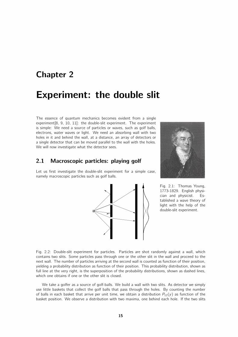
Fig. 2.2: Double-slit experiment for particles. Particles are shot randomly against a wall, whichcontains two slits. Some particles pass through one or the other slit in the wall and proceed to thenext wall. The number of particles arriving at the second wall is counted as function of their position,yielding a probability distribution as function of their position. This probability distribution, shown asfull line at the very right, is the superposition of the probability distributions, shown as dashed lines,which one obtains if one or the other slit is closed.
We take a golfer as a source of golf-balls. We build a wall with two slits. As detector we simplyuse little baskets that collect the golf balls that pass through the holes. By counting the numberof balls in each basket that arrive per unit time, we obtain a distribution P12(y) as function of thebasket position. We observe a distribution with two maxima, one behind each hole. If the two slits
15

16 2 EXPERIMENT: THE DOUBLE SLIT
are close together the two maxima may also merge into one.Let us repeat the experiment with the second slit closed. The golfer shots the balls at the same
rate at the wall with the single remaining slit. This experiment yields a distribution of golf balls P1(y).Then we repeat the experiment with the first hole closed and obtain the distribution P2(y).
For classical particles the three distributions are not independent but they are related by
P12(y) = P1(y) + P2(y) ,
that is the two distributions P1(y) and P2(y) simply add up to P12(y).The explanation for this result is that the ball passes either through one or the other hole. If
it passes through one hole, it does not feel the other hole, and vice versa. Hence, the probabilitiessimply add up.
2.2 Macroscopic waves: water waves
Now, let us turn to waves we understand well, namely water waves.
Fig. 2.3: Double-slit experiment for waves. A source on the left emits waves, which pass throughtwo slits in a first wall. The intensity, which is proportional to the maximum squared amplitude atthe second wall is monitored and shown on the very right. One observes an interference patternfor the intensity as the waves emerging from the two slits interfere. They interfere constructively incertain directions from the double slit, indicated by the dashed lines, leading to a maximum of theintensity, and they interfere destructively in other directions, leading to vanishing intensity. While theamplitudes of the waves emerging from the two slits add up to the total amplitude, the intensitiesobtained, when one or the other slit is closed, do not add up to the total amplitude.
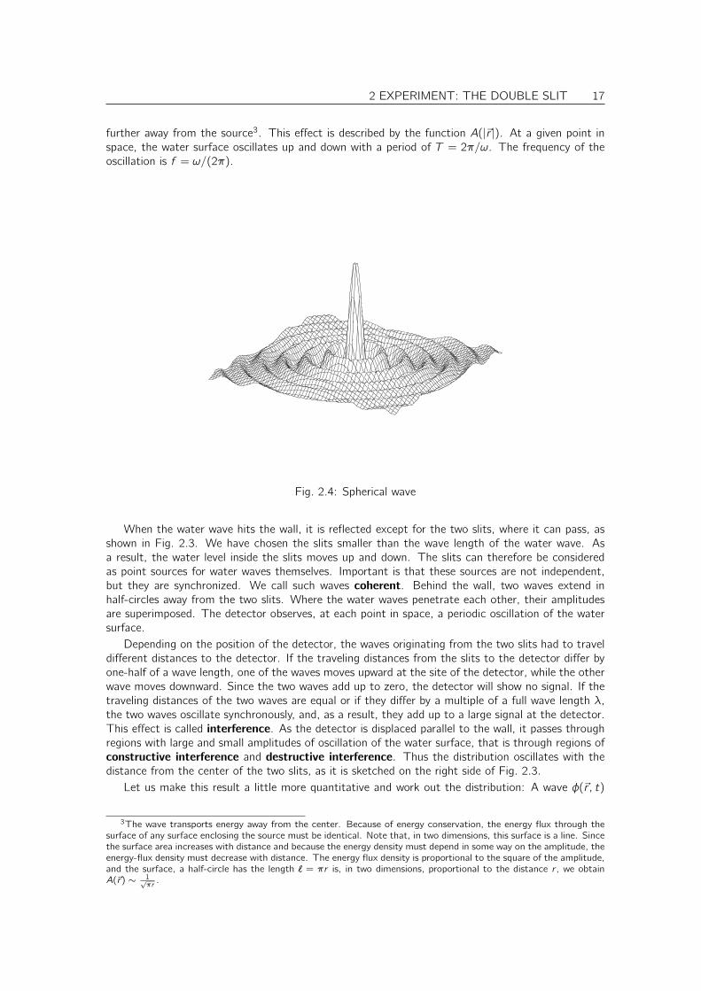
The water wave is created in this experiment by a finger that periodically moves up above anddown below the water surface. The frequency is characterized by the angular frequency ω.1 Thewater wave moves radially outward. The height of the water surface has the form
φ(~r , t) = A(|~r |) sin (k |~r | − ωt) = A(|~r |) sin(k[|~r | −
ω
kt])
(2.1)
It is assumed that the finger is located at the origin of the coordinate system. We see2 that the crestsand troughs of the wave move outward with constant velocity ω/k . The wave crests are separatedby the wave length λ = 2π/k . The amplitude of the oscillations decreases with the distance fromthe source, because the energy of the wave is distributed over a larger region as the wave moves
1The angular frequency is 2π times the frequency or ω = 2π/T where T is the period of the oscillation.2Consider a wave crest, which forms a line defined by those points for which the argument of the sinus has the
value π+ 2πn with an integer n. Hence the line is defined by |~r(t)| = π+2πnk
+ ωkt. Thus the velocity of the wave crest
is v =d |~r(t)|dt
= ωk.
2 EXPERIMENT: THE DOUBLE SLIT 17
further away from the source3. This effect is described by the function A(|~r |). At a given point inspace, the water surface oscillates up and down with a period of T = 2π/ω. The frequency of theoscillation is f = ω/(2π).
Fig. 2.4: Spherical wave
When the water wave hits the wall, it is reflected except for the two slits, where it can pass, asshown in Fig. 2.3. We have chosen the slits smaller than the wave length of the water wave. Asa result, the water level inside the slits moves up and down. The slits can therefore be consideredas point sources for water waves themselves. Important is that these sources are not independent,but they are synchronized. We call such waves coherent. Behind the wall, two waves extend inhalf-circles away from the two slits. Where the water waves penetrate each other, their amplitudesare superimposed. The detector observes, at each point in space, a periodic oscillation of the watersurface.
Depending on the position of the detector, the waves originating from the two slits had to traveldifferent distances to the detector. If the traveling distances from the slits to the detector differ byone-half of a wave length, one of the waves moves upward at the site of the detector, while the otherwave moves downward. Since the two waves add up to zero, the detector will show no signal. If thetraveling distances of the two waves are equal or if they differ by a multiple of a full wave length λ,the two waves oscillate synchronously, and, as a result, they add up to a large signal at the detector.This effect is called interference. As the detector is displaced parallel to the wall, it passes throughregions with large and small amplitudes of oscillation of the water surface, that is through regions ofconstructive interference and destructive interference. Thus the distribution oscillates with thedistance from the center of the two slits, as it is sketched on the right side of Fig. 2.3.
Let us make this result a little more quantitative and work out the distribution: A wave φ(~r , t)
3The wave transports energy away from the center. Because of energy conservation, the energy flux through thesurface of any surface enclosing the source must be identical. Note that, in two dimensions, this surface is a line. Sincethe surface area increases with distance and because the energy density must depend in some way on the amplitude, theenergy-flux density must decrease with distance. The energy flux density is proportional to the square of the amplitude,and the surface, a half-circle has the length ` = πr is, in two dimensions, proportional to the distance r , we obtainA(~r) ∼ 1√
πr.

18 2 EXPERIMENT: THE DOUBLE SLIT
originating from a single point source, such as one of the slits, has the form
φ(~r , t)Eq. 2.1
= A(`) sin(k`− ωt), (2.2)
where ` = |~r − ~r0| is the distance of the detector at position ~r from the point source at ~r0. In ourexperiment the two slits play the role of the point sources.
1
2d
y
x
Fig. 2.5: Demonstration of the variables used for the calculation of the distribution of the doubleslit experiment for classical waves.
The two waves originate from slits separated by a distance d . We denote the distances of the
detector from each slit as `1 =√x2 + (y − d
2 )2 and `2 =√x2 + (y + d
2 )2 respectively. x is thedistance of the screen from the slits and y is the position on the screen relative to the projection ofthe mid plane of the slits. Similarly we denote the wave amplitudes as φ1 and φ2.
In order to design the experiment such that we can compare it with the corresponding particleexperiment, we consider here the intensity of the wave instead of the amplitude.
The intensity is the time averaged energy flux of the wave. We have rescaled the wave amplitudesuch that the proportionality constant between energy flux and half of the squared wave amplitudeis absorbed in the latter. Thus the intensity can be written in the form
I(~r) =1
2
⟨φ2(~r , t)
⟩t
= limT→∞
1
T
∫ T
0
dt1
2φ2(~r , t) (2.3)
The angular brackets denote the time average.

2 EXPERIMENT: THE DOUBLE SLIT 19
Let us now calculate the intensity I12 = 12
⟨12 (φ1 + φ2)2
⟩t
of the superposed waves from the two
slits, where φ1 = A(`1) sin(k`1 − ωt) and φ2 = A(`2) sin(k`2 − ωt).We introduce the mean distance `0
def= 1
2 (`1 +`2) and the difference ∆def= `2−`1, so that `1 = `0−∆/2
and `2 = `0 + ∆/2. Similarly we use the short hand A1def= A(`1) and A2
def= A(`2)
The sinus can be decomposed according to
sin(a + b)Eq. O.4
= sin(a) cos(b) + cos(a) sin(b) , (2.4)
where a = k`0 − ωt and b = ±k∆/2, to obtain
sin(k`0 ± k∆
2− ωt) Eq. 2.4
= sin(k`0 − ωt) cos(k∆
2)± cos(k`0 − ωt) sin(k
∆
2) (2.5)
Similarly we can write
A1 =1
2(A1 + A2) +
1
2(A1 − A2)
A2 =1
2(A1 + A2)−
1
2(A1 − A2) (2.6)
so that we obtain for the superposition of the two waves
φ1 + φ2 = A(`1) sin(k`1 − ωt) + A(`2) sin(k`2 − ωt)Eq. 2.5,Eq. 2.6
= (A1 + A2) sin(k`0 − ωt) cos(k∆/2)
+ (A1 − A2) cos(k`0 − ωt) sin(k∆/2) (2.7)
Now we introduce the following shorthand notations R,S, α
Rdef= (A1 + A2) cos(k∆/2) (2.8)
Sdef= (A1 − A2) sin(k∆/2) (2.9)
cos(α)def= R/
√R2 + S2 (2.10)
sin(α) = S/√R2 + S2 (2.11)
The last relation for the sinus follows directly from the identity cos2(α) + sin2(α) = 1.
φ1 + φ2Eq. 2.7
= R sin(k`0 − ωt) + S cos(k`0 − ωt)
=√R2 + S2
[sin(k`0 − ωt) cos(α) + cos(k`0 − ωt) sin(α)
]Eq. 2.4
=√R2 + S2 sin(k`0 − ωt + α) (2.12)
In the last step we used again Eq. 2.4. cont’d

20 2 EXPERIMENT: THE DOUBLE SLIT
From the last equation we can read that the intensity of the oscillation averaged over time is givenby the squared pre-factor R2 + S2 multiplied by a factor 1/2 that results from the time average ofthe oscillatory part.
I12Eq. 2.3
= limT→∞
1
T
∫ T
0
dt1
2(φ1(t) + φ2(t))2 Eq. 2.12
=1
4
(R2 + S2
)Eqs. 2.8,2.9
=1
4(A1 + A2)2 cos2(k∆/2) +
1
4(A1 − A2)2 sin2(k∆/2)
Eq. O.2=
1
4A2
1 +1
4A2
2 +1
2A1A2(cos2(k∆/2)− sin2(k∆/2))
Eq. O.2=
1
4A2
1 +1
4A2
2 +1
2A1A2(1− 2 sin2(k∆/2))
Eq. O.7=
1
4A2
1︸︷︷︸I1
+1
4A2
2︸︷︷︸I2
+1
2A1A2 cos(k∆))
One factor 12 in the proportionality between intensity and A2 stems from the definition of the intensity
and the other from the time average of the squared sinus function.
INTERFERENCE PATTERN IN THE INTENSITY
Thus we obtain the intensity I12(y)Eq. 2.3
=⟨
12 (φ1(y , t) + φ2(y , t))2
⟩twhen both slits are open as
I12(y) = I1(y) + I2(y) + 2√I1(y)I2(y) cos(k∆(y))︸ ︷︷ ︸
Interference term
(2.13)
from the intensities I1(y) =
⟨12φ
21(y)
⟩t
and I2(y) =
⟨12φ
22(y)
⟩t
that are obtained, when one or the
other slit is closed
∆(y) in Eq. 2.13 is a function 4 that varies monotonously from −d for y = −∞ to +d at y = +∞as shown in Fig. 2.6. Close to the center, that is for y = 0 and if the screen is much farther fromthe slits than the slits are separated, ∆ is approximately ∆(y) = yd/x + O(y2). Hence the spatialoscillation near the center of the screen has a period 5 of 2πx/(kd).
An important observation is that the intensities do not simply add up as the probabilities do forparticles. The first two terms are just the superposed intensities of the contribution of the two slits.If we interpret the intensities as probabilities for a particle to arrive, they correspond to the probabilitythat a particle moves through the left slit and the probability that it moved to the right slit. The
4
∆(y) = `2 − `1 =
√x2 + (y +
1
2d)2 −
√x2 + (y −
1
2d)2 =
√x2 + y2 +
d2
4+ dy −
√x2 + y2 +
d2
4+ dy
=
√x2 + y2 +
d2
4
[√1 +
yd
x2 + y2 + d2
4
−√
1−yd
x2 + y2 + d2
4
]
d<<x,y≈
√x2 + y2
[√1 +
yd
x2 + y2−
√1−
yd
x2 + y2
]Taylor
=√x2 + y2
yd
x2 + y2= d
y√x2 + y2
sin γdef= y√
x2+y2
= sin(γ)d
5The period Λ of cos(k∆(y) is given by k∆(y + Λ) = k∆(y) + 2π. In the center of the screen, i.e. y = 0 and for
small wave length, we can Taylor-expand ∆ and obtain k d∆dy
Λ = 2π. Thus the period is Λ = 2πk
(d∆dy
)−1= 2πx
kd.

2 EXPERIMENT: THE DOUBLE SLIT 21
−20 20−40
∆
d
0 y
−1
1
0
Fig. 2.6: ∆(y) = `2 − `1 for a a double slit with d = 1 and a screen separated from the slit byx = 10. The function ∆ is approximately linear ∆(y) ≈ d/x in the center of the interference pattern,i.e. for y ≈ 0, and it is nearly constant for x >> d . For large deflections, it saturates at a value∆(|y | >> x) = ±d .
last, oscillatory term is a property of waves called interference term.The interference term oscillates more rapidly if the wave length λ = 2π/k becomes small com-
pared to the distance of the slits, i.e. λ << d . This is shown in Fig. 2.7. In the extreme case of avery short wave length, the interference term oscillates so rapidly that the oscillations are averagedout by any experiment that has a finite resolution. In this limit, the oscillations become invisible. Insuch an ’inaccurate’ experiment, the wave intensities behave additive just as probabilities for particles.Hence, waves with very short wave lengths behave in a certain way like particles. Waves with longerwave lengths do not.
DISAPPEARANCE OF THE INTERFERENCE TERM FOR SMALL WAVE LENGTH
In the limit of very small wave length, the interference term is averaged out in any experiment havinga finite resolution. The non-oscillatory term of the intensities, which can still be observed, behavesadditive just like the probability of particles. Thus the wave character of particles disappears in thelimit of short wavelength.
This is a very important result, which lies at the heart of measurement theory and the classicallimit of quantum mechanics that will be described later.
2.3 Microscopic waves: light
Sofar, everything sounds familiar. Now let us switch to the microscopic world and investigate light,which has a much shorter wave length:
The wave length of visible light varies from 750 nm for red light to 400 nm for blue light. Ifthe wave length is longer than for visible light, we pass through infrared, namely heat radiation, tomicrowaves as they are used for radio and mobile telephony. For wave lengths shorter than that ofvisible light, we pass through ultraviolet light up to X-ray radiation. The wave length of visible lightis still large compared to atomic dimensions. Atoms in a crystal have a typical distance of 1-2 Å or0.1-0.2 nm, which is why X-rays need to be used to determine crystal structures.
If we perform the two-slit experiment with light, we need to use photo-detectors. A photo-detector contains electrons loosely bound to defect atoms in a crystal. When such a crystal is placedin an electric field, such as that of a light beam, the electrons can follow the applied electric field,resulting in a measurable current.

22 2 EXPERIMENT: THE DOUBLE SLIT
0 10−10 −5 5
Fig. 2.7: Interference pattern of a two dimensional wave through a double slit with separationd = 5, on a screen located at a distance z = 1 behind the slits. The wave length has valuesλ = 0.2, 2, 20, 200 with increasing values from the bottom to the top. Each figure contains inaddition the sum of intensities from the individual slits (yellow dashed line), which would correspondto a pure particle picture.
Let us now return to the double-slit experiment. For a regular light source, we obtain the sameinterference pattern as for water waves, only a lot smaller in its dimensions.
What happens as we slowly turn down the light? At first, the intensity measured by the photodetector becomes smaller, but the signal maintains its shape. If we turn the light further down, afterthe intensity is far too small to be observed with the naked eye, the signals begins to flicker andfor even lower intensity random independent flashes of very low intensity are observed. If we use anarray of photo detectors at different positions, only one detects a flash at a time, while the othersare completely silent. (The experimentalists assured me that this is not a problem with their photodetectors.) If we add up the signals over time, the original interference pattern is observed.
Thus if the light is turned down, it behaves lumpy, like particles! These particles are calledphotons.
Apparently, if the light is strong, many photons are detected in short time intervals, so that weobtain a signal that appears continuous. In reality we see many particles. Thus our experience hasmisguided us, and we have introduced a concept of a continuous wave, even though we actuallyobserve particles.
2.4 Microscopic particles: electrons
Let us now go to the microscopic world of particles. We choose electrons as example. We mount asmall metallic tip so that it points towards a metallic plate that has two slits in it. Between tip andmetal plate we apply a large voltage. Near the tip the electric field becomes so large, that it ripselectrons out of the tip, which in turn travel towards the metallic plate. The metallic plate has twoslits, which allows some electrons to pass through.
Electrons that pass through the slits are collected by a detector. We count the electrons thatarrive at the detector, when the detector is at a given position. The electrons pass one by one, andenter the detector as individual particles, but when we count a large number of them as a function ofposition of the detector, we obtain a clear interference pattern as in the case of light! This is shown

2 EXPERIMENT: THE DOUBLE SLIT 23
in Fig. 2.8.
Fig. 2.8: Results of a double-slit-experiment performed by Dr. Tonomurashowing the build-up of an interferencepattern of single electrons. Numbers ofelectrons are 10 (a), 200 (b), 6000 (c),40000 (d), 140000 (e).[12, 11, 13]
We remember that the interference pattern for waterwaves resulted from the wave passing through both holessimultaneously. We expect that a particle, which passesthrough either one or the other hole cannot have an inter-ference pattern.
Let us change the experiment. We close one hole,collect the signals, then close the other, and add up thesignals. The result are two maxima, but no interferencepattern. Apparently there is not only the possibility thatthe particle passes through one or the other slit, but alsothe probability that it passes through both slits simultane-ously. The latter possibility makes the difference betweenthe two humps, which are expected for particles, and theinterference pattern, expected for waves.
A movie and demonstration of the double-slit experi-ment can be found at the Hitachi Web site http://www.hqrd.hitachi.co.jp/em/doubleslit.cfm
2.5 Summary
We have learned that waves such as light are composed offixed quanta, which we may identify with particles. Par-ticles such as electrons on the other hand are wavy intheir collective behavior. In the macroscopic world, eitherthe particle properties or the wave properties dominate, sothat we have developed two different concepts for them.In reality they are two aspects of the same concept, whichis the realm of quantum theory.
The observations of the double-slit experiment cannotbe derived from any theory of classical waves or classicalparticles independently. What we observe is a new phe-nomenon. A new theory is required, and that theory isquantum theory. Together with Einstein’s theory of rel-ativity, the advent quantum theory changed radically ourview of the world in the early 20th century.
2.6 Recommended exercises
1. Interference: Exercise 16.1 on p. 235

24 2 EXPERIMENT: THE DOUBLE SLIT

Chapter 3
Towards a theory
Fig. 3.1: ErwinSchrödinger, 1887-1961.Photograph from 1933.Austrian Physicist. Nobelprice 1933 in physics forthe Schrödinger equation.
In the previous section, we learned that particle beams exhibit interfer-ence patterns as they are known from waves. To be more precise, theprobability of finding a particle at a point in space exhibits an interfer-ence pattern. Therefore, we need to construct a theory that on the onehand is able to describe interference patterns on a small length scale andon the other hand it must match classical mechanics on a macroscopiclength scale. One possibility is to consider particles as wave packets. Ifthe size of the wave packet and the wave length is small on macroscopiclength scales, we may be fooled in thinking that the particle is in fact apoint. On the other hand, the wavy nature may reveal itself on a lengthscale comparable to the wave length.
In the following, we will try to find a theory of waves in the form ofdifferential equations, in which wave packets behave, on a macroscopiclength scale, like classical particles.
3.1 Particles: classical mechanics revisited
Before we investigate the behavior of wave packets, let us revisit themain features of classical mechanics. One requirement of our theory isthat the wave packets behave like classical particles, if the wave lengthis small. Therefore, we first need to have a clear understanding of the dynamics of classical particles.
In classical mechanics, the motion of particles is predicted by Newton’s equations of motion
m..x = F = −∂xV (x)
where each dot denotes a time derivative, and ∂xV is the derivative of the potential V (x) with respectto the position x . Newton’s equations relates the acceleration
..x of a particle to the force F acting
on the particle with the mass m as proportionality constant.The equations of motion can be derived from another formalism, the principle of least action1.
The principle of least action is particularly useful to obtain a consistent set of forces from, for example,symmetry arguments.
We start from a so-called Lagrangian L(v , x), which depends on positions x and velocities v =.x .
For a particle in a potential, the Lagrangian has the form kinetic energy minus potential energy
L(v , x) =1
2mv2 − V (x)
1“principle of least action” translates as “Wirkungsprinzip; Hamilton principle” into German
25

26 3 TOWARDS A THEORY
The principle of least action says that from all conceivable paths x(t) starting at time t1 from x1
and arriving at time t2 at their destination x2, the particle will choose that path which minimizes theaction S.2 The action is a functional 3 of the path defined as follows:
ACTION
The action S is a functional of a path x(t). It is the integral of the Lagrangian L over a path
S[x(t)] =
∫ x2,t2
x1,t1
dt L(.x, x) (3.1)
The integration bounds indicate that the path begins at a specified space-time point (x1, t1) andends at another one, namely (x2, t2). When the path is varied within the framework of the principleof least action, these boundary conditions remain unchanged.
x(t)+ x(t)δ
δx(t)
x(t)
x
t
(x1,t1)
(x2,t2)
Fig. 3.2: Two paths, x(t) and x(t) + δx(t), connecting two space-time points, (x1, t1) and (x2, t2).Each path has a different value for the action S[x(t)]. The action depends on the path as a whole.If the action does not change to first order with respect to all possible small variations δx(t), theaction is stationary for this path, and the path is a physical trajectory from the initial to the finalpoints.
The minimum, or better a stationary point, of the action is obtained as follows: We consider apath x(t) and a small variation δx(t). The variation δx(t) vanishes at the initial and the final time.Now we test whether an arbitrary variation δx(t) can change the action to first order. If that is not
2One should better say that the physical path makes the action stationary rather than minimize it. Historically thismore general formulation has been noticed only long after the principle of least action has been formulated, so that weoften speak about minimizing the action, even though this statement is too limited.
3A functional maps a function onto a number. To show the analogy, a function maps a number onto a number. Afunctional can be considered a function of a vector, where the vector index has become continuous.

3 TOWARDS A THEORY 27
the case, the action is stationary for the path x(t).
S[x(t) + δx(t)] =
∫dt L(
.x + δ
.x, x + δx)
Taylor=
∫dt[L(.x, x) +
∂L∂vδ.x +
∂L∂xδx +O(δx2)
]part. int.
= S[x(t)] +
∫dt[ ddt
(∂L∂vδx)−( ddt
∂L∂v
)δx +
∂L∂xδx +O(δx2)
]= S[x(t)] +
[∂L∂vδx]x2,t2
x1,t1︸ ︷︷ ︸=0
+
∫dt[−( ddt
dLdv
)+dLdx
]δx(t) +O(δx2)
δS = S[x(t) + δx(t)]− S[x(t)] =
∫dt[−( ddt
∂L∂v
)+∂L∂x
]δx +O(δx2)
Thus, the functional derivative of the action is
δSδx(t)
= −( ddt
∂L∂v
)+∂L∂x
(3.2)
The notation O(δx2) is a short hand notation for all terms that contains the second and higherpowers of δx .
The derivation contains the typical steps, which are worth to remember:(1) Taylor expansion of the Lagrangian to first order in coordinates and velocities.(2) Conversion of derivatives δ
.x into δx using partial integration.
(3) Removing the complete derivatives using boundary conditions δx(t1) = δx(t2) = 0.The requirement that dS = S[x + δx ] − S[x ] vanishes for any variation δx in first order of δx ,
translates, with the help of Eq. 3.2, therefore into the
EULER-LAGRANGE EQUATIONS
d
dt
∂L(v , x)
∂v=∂L(v , x)
∂xwith v =
.x (3.3)
The Euler-Lagrange equations are identical to Newton’s equation of motion which is easily verifiedfor the special form L = 1
2mv2 − V (x) of the Lagrangian.
3.1.1 Hamilton formalism
The Hamilton formalism is identical to the principle of least action, but it is formulated in moreconvenient terms. Noether’s Theorem4[14] says that every continuous symmetry results in a con-served quantity. For a system that is translationally symmetric in space and time, the two conservedquantities are momentum and energy, respectively. The Hamilton formalism is built around thosetwo quantities.
The Hamilton formalism is obtained by a Legendre transformation of the Lagrangian. We definea new function, the Hamilton function
4see ΦSX: Klassische Mechanik
28 3 TOWARDS A THEORY
HAMILTON FUNCTION
H(p, x)def=pv − L(v , x, t), (3.4)
The Hamilton function depends on positions and momenta p, but not on on the velocities! Asdescribed in the following, the velocities are considered a function v(p, x) of momenta and coordinatesthemselves, i.e.
H(p, x) = p · v(p, x, t)− L(v(p, x, t), x, t),
The physical meaning of the Hamilton function is the total energy.
In order to get rid of the dependence on the velocity v in Eq. 3.4, we define the momentum p sothat the Hamilton function H does not explicitly depend on
.x . This leads to
∂H∂v
= p −∂L∂v
= 0
which defines the canonical momentum as follows:
CANONICAL MOMENTUM
pdef=∂L∂v
(3.5)
The difference between the canonical momentum described above and the kinetic momentum de-fined as p′ = mv , that is as mass times velocity. The kinetic momentum is the canonical momentumof a free particle.
From Eq. 3.5 we obtain the momentum p(x, v , t) as function of positions and velocities. Thisexpression can be converted into an expression for the velocity v(p, x, t) as function of momenta andpositions. The latter is used in Eq. 3.4 to obtain the Hamilton function.
In the following, we derive a new set of equations of motion by forming the derivatives of theHamilton function with respect to positions and momenta and by using the Euler Lagrange equationsEq. 3.3. The resulting equations of motion are called Hamilton’s equations. Hamilton equations,contain exactly the same information as Newton’s equation of motion and the Euler-Lagrange equa-tions.
∂H∂x
Eq. 3.4= −
∂L∂x
+
(p −
∂L∂v
)︸ ︷︷ ︸
= ∂H∂v
=0
∂v(p, x)
∂x
Eq. 3.3= −
d
dt
∂L∂v
Eq. 3.5= −.p
∂H∂p
Eq. 3.4= v +
(p −
∂L∂v
)︸ ︷︷ ︸
= ∂H∂.x
=0
∂v(p, x)
∂p= v =
.x
We generalize the result to higher dimensions

3 TOWARDS A THEORY 29
HAMILTON’S EQUATIONS OF MOTION
.pi = −
∂H∂xi
.x i =
∂H∂pi
(3.6)
We will come back to the Hamilton equations in quantum mechanics, when we investigate the dy-namics of wave packets. Euler-Lagrange equations, Hamilton equations and Newton’s equations ofmotion have the same content and are mathematically identical.
3.2 Waves: the classical linear chain
Let us now remind ourselves of some properties of classical waves. As a working example, I amchoosing the most simple wave I can think of, namely the vibrations of a linear chain. The linearchain consists of particles, or beads, distributed along a line. The beads are free to move along thedirection of the line, but each bead is connected to the two neighboring beads by springs.
The linear chain is a simple model for lattice vibrations, where atoms oscillate about some equilib-rium positions. If an atom in a crystal is displaced, the bonds to the neighboring atoms are stretchedon one side and compressed on the other. The resulting forces try to restore the original atomicdistances. If we let the beads loose, they will start to oscillate. These oscillations usually propagatealong the entire chain. If we consider the material on a larger length scale, and if we ignore that thematerial is made of individual atoms, we can consider those lattice deformations as continuous wavessimilar to water waves or light. These lattice-distortion waves are called phonons. Phonons are thequanta of lattice vibrations just as photons are the quanta of light.
• Phonons are used to describe the transport of sound waves in solids.
• Phonons are responsible for heat transport in insulators. (In metals the electronic contributionto the heat transport is usually a lot larger than the lattice contribution.)
3.2.1 Equations of motion ...
jxjφ
αm
∆
Let us now describe the linear chain mathematically:The positions of the particles are at xj(t) = xj + φj(t). The equi-
librium positions xj = j∆ are equally spaced with a distance ∆ betweenneighboring particles. The displacements from the equilibrium positionsare denoted by φj(t).
Let us write down the Lagrangian, from which we obtain the equa-tions of motion. The Lagrangian is kinetic energy minus potential en-ergy.
L(.φj, φj) =
∑j
[1
2m.φ
2
j −1
2α(φj − φj−1)2
](3.7)
α is the spring constant. Thus the energy of a spring is 12α(d − d0)2, where d = xj − xj−1 is the
actual length of the spring and d0 = xj − xj−1 is the length of the spring without tension.

30 3 TOWARDS A THEORY
The action is defined as the integral of the Lagrange function.
S [φj(t)] =
∫ φ2,j,t2
φ1,j,t1
dt L(.φj(t), φj(t))
We use curly brackets to denote all elements in a vector, and brackets to denote functions. Theaction is a functional of the time-dependent displacements [φj(t)]. According to the variationalprinciple, the physical displacements φj(t) are the extremum of the action under the condition thatthe displacements at the initial time t1 and the final time t2 have fixed values.
We determine the equations of motion for the displacements φj(t) from the extremum condition,that is the Euler-Lagrange equations Eq. 3.3.
d
dt
∂L
∂.φn
Eq. 3.3=
∂L∂φn
Eq. 3.7⇒d
dt
(m.φn
)=
∂
∂φn
(−
1
2α(φn − φn−1)2 −
1
2α(φn+1 − φn)2
)⇒ m
..φn = −α(φn − φn−1) + α(φn+1 − φn)
⇒ m..φn = α (φn+1 − 2φn + φn−1) (3.8)
The right hand side reminds of the differential quotient of the second derivative. 5
3.2.2 ... and their solutions
The equations of motion Eq. 3.8 are those of a multidimensional harmonic oscillator, since the forcesare linear in the displacements φn. The multidimensional harmonic oscillator can be solved withthe techniques described in ΦSX: Klassische Mechanik[14].
The problem Eq. 3.8 is even simpler than the multidimensional harmonic oscillator, because itis translationally invariant. Translationally invariant problems are best solved with an exponentialAnsatz.
φj(t) =
∫dk
2πa(k)ei(kxj−ω(k)t) (3.9)
We insert this Ansatz into the equations of motion Eq. 3.8 for the linear chain. This will provideus with the dispersion relation of the linear chain. A dispersion relation relates the frequency ω(k)to the wave vector k . Another form of the dispersion relation connects the energy of a particle to itsmomentum. Later, we will see that there is an intimate connection between energy and frequencyon the one hand and the momentum and the wave vector on the other hand.
m..φn
Eq. 3.8= α (φn+1 − 2φn + φn−1)
Eq. 3.9⇒∫dk
2π(−mω2(k))a(k)ei(kxn−ωt) =
∫dk
2πα (eik∆ − 2 + e−ik∆)︸ ︷︷ ︸[
eik∆2 −eik
∆2
]2
=(2i)2 sin2(k ∆2
)
a(k)ei(kxn−ωt)
mω2(k) = 4α sin2(k∆
2)
ω(k) = ±2
√α
msin(
k∆
2) (3.10)
5Differential quotient of the second derivative
d2f
dx2= lim
∆→0
f (x + ∆)− 2f (x) + f (x − ∆)
∆2

3 TOWARDS A THEORY 31
Eq. 3.10 is the dispersion relation of the linear chain. Its graph is shown in Fig. 3.3. Like the dispersionrelation of light, the one of the linear chain behaves almost linear for small wave vectors. In contrastto light, however,the linear chain has a maximum angular frequency6 of ωmax = 2
√α/m. This is a
consequence of the discrete nature of the linear chain.
−3
−2
−1
0
1
2
3
−1.5 −1 −0.5 0 0.5 1 1.5
ω/√
αm
∆2 k
Fig. 3.3: Dispersion relation ω(k) of the discrete linear chain. The straight (dotted) lines are thedispersion relation of a continuous linear chain. The dispersion relation of the discrete chain is periodicwith period 2π
∆ . (Each branch by itself has a period of 4π∆ .)
With the dispersion relation Eq. 3.10, we can write down the solution Eq. 3.9 for the linear chainas
φj(t) =
∫dk
2π
(a+(k)ei(kxj−|ω(k)|t) + a−(k)ei(kxj+|ω(k)|t)
)with
a+(k) = a−(−k)∗
The last requirement ensures that the displacements are real. 7
Usually, we can work with each component independently of the other. The coefficients a±(k)are determined from the initial conditions.
φj(t = 0) =
∫dk
2π(a+(k) + a−(k))eikxj
∂tφj(t = 0) = −∫dk
2πi |ω(k)|(a+(k)− a−(k))eikxj
6The angular frequency ω is defined as
ω =2π
T= 2πf (3.11)
where T is the duration of a period and f = 1/T is the frequency.7Here we show that the requirement that a field has only real values implies the relation a(k) = a∗(−k) of its
Fourier components: Let φj = φ(xj ), where xj = ∆j . The requirement that the displacements φ(x) are real has theform
φ(x) = φ∗(x)φj=
∫ dk2π eikx a(k)⇒
∫dk
2πeikxa(k) =
∫dk
2πe−ikxa∗(k)︸ ︷︷ ︸
=∫ dk
2π eik∆j a∗(−k)
⇒∫dk
2πeikx
(a(k)− a∗(−k)
)= 0 ⇒ a(k) = a∗(−k)
q.e.d.

32 3 TOWARDS A THEORY
3.3 Continuum limit: transition to a field theory
Sofar, the linear chain has been formulated by discrete beads. For our purposes, the discrete natureof the chain is of no interest.8 Therefore, we take the continuum limit ∆→ 0 of the linear chain. Inthis way make the transition to a field theory.
We start out with the Lagrangian Eq. 3.7 for the discrete linear chain, and modify it introducingthe equilibrium distance ∆ at the proper positions without changing the result.
L(∂tφj, φj)Eq. 3.7
= lim∆→0
∑j
∆︸ ︷︷ ︸→∫dx
[1
2
m
∆︸︷︷︸→%
(∂tφj)2 (t)−
1
2α∆︸︷︷︸→E
(φj(t)− φj−1(t)
∆
)2
︸ ︷︷ ︸→(∂xφ)2
]
As ∆ approaches zero, we can convert the sum into an integral and the differential quotient willapproach the derivative. We also see that a meaningful limit is obtained only if the mass is scaledlinearly with ∆, that is m(∆) = %∆ and if the spring constant is scaled inversely with ∆, that isα(∆) = E
∆ . % is the mass density of the linear chain and E is its linear elastic constant9. Thusthe potential-energy term in the Lagrangian can be identified with the strain energy. Finally, thedisplacements φj(t) of the individual beads must be replaced by a displacement field φ(x, t) so thatφ(xj , t) = φj(t) for xj = j∆.
The limit ∆→ 0 then yields
L[φ(x), ∂tφ(x)] =
∫dx
[1
2% (∂tφ(x))2 −
1
2E(∂xφ(x))2
]cdef=√E%
=1
2E∫dx
[1
c2(∂tφ(x))2 − (∂xφ(x))2
](3.12)
where we have introduced the speed of sound c =√E% . The identification of c with the speed of
sound will follow later from the Euler-Lagrange equation and the corresponding dispersion relation.The Euler-Lagrange equations for fields are only slightly more complicated compared to those for
particles. First we extract the Lagrangian density `. The spatial integral of the Lagrangian densityyields the Lagrange function and the integral over space and time yields the action.
For the linear chain, the Lagrangian density is
`(φ, ∂tφ, ∂xφ, x, t) =E2
[ 1
c2(∂tφ)2 − (∂xφ)2
](3.13)
EULER-LAGRANGE EQUATIONS FOR FIELDS
The Euler-Lagrange equations for fields have the form (see ΦSX: Klassische Mechanik[14])
∂t∂`
∂(∂tφ)+ ∂x
∂`
∂(∂xφ)−∂`
∂φ= 0 (3.14)
For the linear chain, we obtain the following equations of motion from Eq. 3.14
1
c2∂2t φ(x, t) = ∂2
xφ(x, t)
8Our ultimate goal is to develop a field theory for particles in free space. Since space and time do not exhibit anystructure, we can as well consider an infinitely fine-grained linear chain.
9The elastic constant (or Young modulus) E = σ/ε is the ratio between stress σ and strain ε. The strain is therelative displacement per unit length. The stress is the force per area that is to be applied to a solid bar. Whereas theelastic constant of a tree-dimensional object has the unit of pressure or “energy-divided-by-volume”, what we call linearelastic constant has the unit “energy-divided-by-length”.

3 TOWARDS A THEORY 33
and the dispersion relation
ω = ±ck
If we compare this dispersion relation with that of the discrete chain in Fig. 3.3, we see that thecontinuum limit is identical to the k → 0 limit of the discrete chain, which is the long wave lengthlimit.
3.4 Differential operators, wave packets, and dispersion rela-tions
Let us now investigate the dynamics of a wave packet. In order to show the full generality of theargument, we start from a general linear differential equation of a translationally invariant system inspace and time.
For a translationally invariant system, the corresponding time and space coordinates do not ex-plicitly enter the differential operator, but only derivatives.10 Hence the differential equation of sucha system has the form11:
Q(∂t , ∂x)φ(x, t) = 0
In the special case of the continuous linear chain discussed before, the function Q has the formQ(a, b) = 1
c2 a2 − b2 so that the differential operator has the form Q(∂t , ∂x) = 1
c2 ∂2t − ∂2
x .12,13
The Ansatz φ(x, t) = ei(kx−ωt) converts the differential equation of a translationally invariantsystem into an algebraic equation, because
∂tei(kx−ωt) = −iωei(kx−ωt)
∂xei(kx−ωt) = +ikei(kx−ωt) (3.15)
so that
0 = Q(∂t , ∂x)ei(kx−ωt) = Q(−iω, ik)ei(kx−ωt)
Resolving the equation Q(−iω, ik) = 0 for ω yields the dispersion relation ωσ(~k), which providesthe angular frequency ω as function of the wave vector k . Depending on the order14 of the differentialequation with respect to time, we may obtain one or several solutions ω for a given k . Thus thedispersion relation may have several branches, which we denote by an index σ.
In the special case of the continuous linear chain Q(−iω, ik) = −ω2
c2 + k2, so that the dispersionrelation has two branches, namely ω1 = ck and ω2 = −ck .
The most general solution of the differential equation is then
φ(x, t) =∑σ
∫dk
2πei(kx−ωσ(k)t)aσ(k) (3.16)
with some arbitrary coefficients aσ(k). Once the initial conditions are specified, which determineaσ(k), we can determine the wave function for all future times.
10Any dependence on x or t in the differential operator would imply that it is not invariant with respect to thecorresponding translations. The differential operator is called translationally invariant, if a shifted solution of thedifferential equation is again a solution of the same differential operator.
11Any differential equation of two variables x and t can be written in the form Q(x, t, ∂x , ∂t)φ(x, t) = 0, whereQ(x, t, u, v) is an arbitrary function of the four arguments. The differential operator is defined by the power seriesexpansion, where u is replaced by ∂x and v is replaced by ∂t
12Here we use a strange concept, namely a function of derivatives. The rule is to write out the expression as if thederivative were a number, but without interchanging any two symbols in a product, because ∂xx 6= x∂x . Note that∂xx = 1 + x∂x , because in operator equations we should always consider that this operator is applied to a function, i.e.∂xxf (x) = f (x) + x∂x f (x) = (1 + x∂x )f (x). Any differentiation occurring in a product acts on all symbol multipliedto it on its right-hand side.
13The operator def= 1
c2 ∂2t − ~∇2 is called the d’Alambert operator. The Laplacian is defined as ∆
def= ~∇2.
14The order of a differential equation is the highest appearing power of a derivative in a differential equation.

34 3 TOWARDS A THEORY
Wave packets
Let us now investigate the behavior of a wave packet. We select an envelope function χ(x, t = 0),a wave vector k0 and one particular branch, i.e. σ, of the dispersion relation.
WAVE PACKET
A wave packet has the form
φ(x, t) = ei(k0x−ωσ(k0)t)χ(x, t) (3.17)
An example is shown in Fig. 3.4. We call χ(x, t) the envelope function. The envelope functionmodulates a plane wave. k0 is the dominating wave vector. We usually assume that the envelopefunction is smooth and extended over several wave lengths λ = 2π/|k0| of the plane wave part.
We want to investigate the behavior of the dynamical evolution of an envelope function χ(x, t).By equating
ei(k0x−ωσ(k0)t)χ(x, t)Eq. 3.17
= φ(x, t)Eq. 3.16
=
∫dk
2πei(kx−ωσ(k)t)aσ(k)
we obtain a expression of χ(x, t)
χ(x, t) =
∫dk
2πei(
[k−k0]x−[ωσ(k)−ωσ(k0)]t)aσ(k) (3.18)
This is an exciting result: For a system, that is translationally invariant in space and time, thedispersion relation is sufficient to predict the complete future of a wave packet.
ψ ψ
x
χ( , )tkψ( , )k t
k0
ψ( , )x t
ei(k0 ωx− t)
k−k0
λ
k
x tχ( , )
2πδ( )
vgr
vph
Fig. 3.4: Wave packet in real and reciprocal space. In real space, a wave packet Ψ(x, t) is theproduct between a plane wave ei(kx−ωt) and a smooth envelope function χ(x, t). The plane wavemoves with the phase velocity vph, while the envelope function moves with the group velocity vgr . Inreciprocal space, the plane wave part is a δ-function times 2π centered at the dominant wave vektork0. Because the envelope function is smooth, it contributes only near k = 0. The wave packetΨ(k, t) is a convolution Ψ(k, t) =
∫dk ′
2π 2πδ(k − k0 − k ′)χ(k ′, t) = χ(k − k0, t).
Sofar, everything has been exact. Now, we need to introduce an approximation that is only validfor very smooth envelope functions χ(x, t) . We assume that the envelope function is smooth on thelength scale of the wave length λ = 2π/k . This implies that its Fourier transform aσ(k) has largecomponents only for k close to |k0|.15 In this region, we can replace ω(k) by its Taylor expansion16
15If f (x) =∫dk2πf (k)eikx then we find by variable substitution x → αx and k → k/α that f (αx) =
∫dk2π
1αf ( k
αx)eikx .
If α becomes smaller f (αx) becomes smoother in real space and more localized near k = 0 in k-space.16The notation O(xn) is a shorthand notation for all terms containing powers of x of order n and higher.

3 TOWARDS A THEORY 35
ω(k) ≈ ω(k0) + dωdk |k0 (k − k0) +O(k − k0)2 to first order in k − k0.
χ(x, t)Eq. 3.18≈
∫dk
2πei [k−k0](x− ∂ωσ
∂kt)aσ(k)
Eq. 3.18= χ(x −
∂ω
∂k︸︷︷︸vg
t, 0) (3.19)
Thus, the wave packet moves with the so-called group velocity vg = ∂ω∂k , without much of a change
of its shape.Let us generalize the result to three dimensions.
GROUP VELOCITY
The wave packet as a whole, i.e. its envelope function, moves with velocity
~vgEq. 3.19
= ~∇~k∣∣∣~k0
ω(~k) or vg,i =∂ω
∂ki
∣∣∣∣~k0
(3.20)
It is not quite true that the wave packet does not change its shape. If we violate the assumptionthat the wave packet is very extended and consider envelope functions that are less smooth, thenthe Fourier transform is no more localized around k0, and higher order terms of the Taylor expansionof ωσ(~k) become important. These terms contribute to a delocalization, or spreading, of the wavepacket. This effect can be thought of in the following way: The wave packet consists of componentswith different velocities, so that faster components run ahead and the slower components lag behindthe rest of the wave packet. As a result, the wave packet usually broadens with time. This broadeningof the wave packet is called dispersion.
In general, the group velocity is distinct from the phase velocity. The phase velocity is derivedfrom a single plane wave
ei(kx−ωt) = eik(x−
vp︷︸︸︷ω
kt)
(3.21)
The phase velocity is the velocity of a single wave crest or wave trough.Again, we list here the three-dimensional expression for the phase velocity
PHASE VELOCITY
~vpEq. 3.21
=ω(~k0)
|~k0|~ek0 =
ω(~k0)
|~k0|
~k0
|~k0|(3.22)
where ~ek = ~k/|~k | is the unit vector pointing along the wave vector ~k . The phase velocity is thevelocity of a wave crest. It can be read from the dispersion relation ω(k) as the slope of the lineconnecting the origin with a particular point at the dispersion relation.
The dispersion relation of the continuous linear chain is purely linear, which implies that thewaves have a constant uniform velocity. This velocity is the velocity of sound, and it is analogous tothe speed of light. A medium with a linear dispersion relation is convenient for signal transmissionbecause, given a constant value for ω/k , a wave packet does maintain its shape during time evenif it is localized in space. Hence, the information encoded in the shape of the wave packet remainsintact during transmission.
3.5 Breaking translational symmetry
The wave packets discussed so-far move with a constant speed. This is a consequence of thetranslational symmetry we have imposed. In order to explore, how we can teach wave packets to
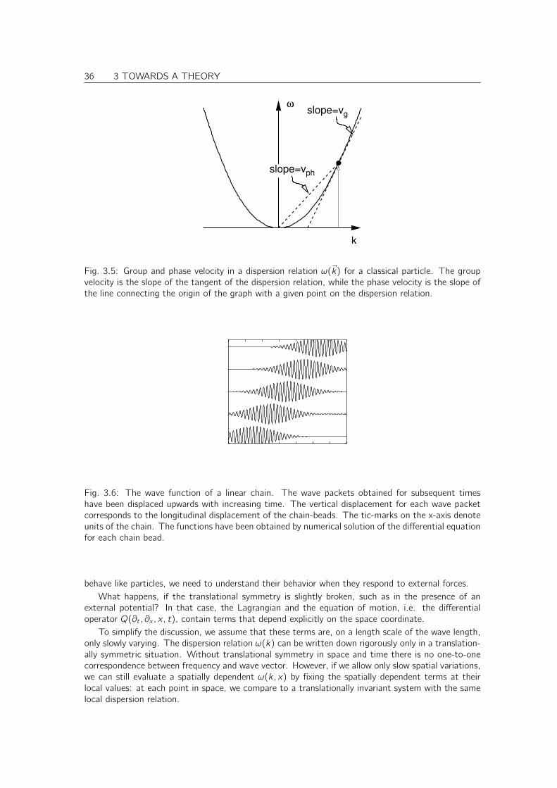
36 3 TOWARDS A THEORY
slope=vph
slope=vg
ω
k
Fig. 3.5: Group and phase velocity in a dispersion relation ω(~k) for a classical particle. The groupvelocity is the slope of the tangent of the dispersion relation, while the phase velocity is the slope ofthe line connecting the origin of the graph with a given point on the dispersion relation.
600 1100
Fig. 3.6: The wave function of a linear chain. The wave packets obtained for subsequent timeshave been displaced upwards with increasing time. The vertical displacement for each wave packetcorresponds to the longitudinal displacement of the chain-beads. The tic-marks on the x-axis denoteunits of the chain. The functions have been obtained by numerical solution of the differential equationfor each chain bead.
behave like particles, we need to understand their behavior when they respond to external forces.What happens, if the translational symmetry is slightly broken, such as in the presence of an
external potential? In that case, the Lagrangian and the equation of motion, i.e. the differentialoperator Q(∂t , ∂x , x, t), contain terms that depend explicitly on the space coordinate.
To simplify the discussion, we assume that these terms are, on a length scale of the wave length,only slowly varying. The dispersion relation ω(k) can be written down rigorously only in a translation-ally symmetric situation. Without translational symmetry in space and time there is no one-to-onecorrespondence between frequency and wave vector. However, if we allow only slow spatial variations,we can still evaluate a spatially dependent ω(k, x) by fixing the spatially dependent terms at theirlocal values: at each point in space, we compare to a translationally invariant system with the samelocal dispersion relation.

3 TOWARDS A THEORY 37
Let us define the position of the wave packet as17.
x0(t)def=
∫dx |φ(x, t)|2x∫dx |φ(x, t)|2
(3.23)
The mean k-vector is denoted by k0. The velocity of the wave packet is the group velocity
∂tx0(t)Eq. 3.20
=∂
∂kω (x0(t), k0(t)) . (3.24)
Since we still have translational symmetry in the time variables, the value of the conjugate variableω(x0(t), k0(t)) remains constant18, so that
0 =d
dtω(x0(t), k0(t)) =
∂ω
∂x∂tx0︸︷︷︸∂ω∂k
+∂ω
∂k∂tk0
Eq. 3.20=
∂ω
∂k
(∂ω∂x
+ ∂tk0
)
⇒ ∂tk0 = −∂
∂xω(x0(t), k0(t)) (3.25)
Let us take a closer look at what we have got: the wave packet travels according to
∂tx0Eq. 3.24
=dω
dk; ∂tk0
Eq. 3.25= −
dω
dx(3.26)
This sounds familiar! Let us compare this result with Hamilton’s equation of motion, Eq. 3.6, forclassical particles
∂tx =dHdp
; ∂tp = −dHdx
(3.27)
The two sets of equations, Eq. 3.26 and Eq. 3.27, are identical, if we perform the replacement
H(p, x)→ ~ω(x, ~k)
p → ~k
where ~ is some arbitrary constant, which we will later identify with the reduced Planck constant.(We have dropped here the subscripts of x and k .)
What we have done sofar, is to derive the equations of motion for wave packets from a specifieddifferential operator. We have seen that the dynamics of wave packets is identical to that of classicalparticles, if the dispersion relations are related.
We are almost there!
17Consider P (x) =|φ(x)|2∫dx |φ(x)2| as a density. Then the definition of the local position is the average position.
18 I have not really explained why ω is conserved with time. Let us assume a differential equationQ(∂t , ∂x , x)Ψ(x, t) = 0. We can then make an Ansatz Ψ(x, t) = e−iωtφ(x, ω). Inserting the Ansatz into the dif-ferential equation yields Q(−iω, ∂x , x) = 0. For each value of ω, we obtain one or more solutions φσ(x, ω). Thegeneral solution can therefore be written as Ψ(x, t) =
∑σ
∫dω2πφσ(x, ω)aσ(ω)eiωt with some arbitrary coefficients aσ.
Thus if we choose the coefficients so that only a small ω-region contributes, this region will be the same for all times.Hence, ω does not change in time.

38 3 TOWARDS A THEORY
CORRESPONDENCE PRINCIPLE
In order to construct wave packets that behave like classical particles, we start from a LagrangianL for the classical particle. From the Lagrangian we derive the Hamilton function H. The equationE −H(p, x) = 0 is converted with the help of Eq. 3.15 into a differential equation by replacing
E → ~ω → i~∂t
p → ~k →~i∂x (3.28)
Hdef= H( ~i ∂x , x) is called the Hamilton operator. The correspondence principle was invented by de
Broglie in his PhD thesis. It is also called de Broglie relation[7].The correspondence principle is used to translate the classical equations of motion into the quantummechanical wave equations and vice versa.
The correspondence principle, when applied to the classical equation E = H(p, x), directly leadsto the
SCHRÖDINGER EQUATION [15, 16, 17, 18]
Q(∂t , ∂x , x, t)ψ(x, t) = [i~∂t −H(~i∂x , x, t)]ψ(x, t) = 0 (3.29)
I introduced a new symbol, namely ψ(x, t) instead of φ(x, t), in order to distinguish the displacementfield φ of a linear chain from the Schrödinger wave function ψ .19
We found a theory that is capable of describing the interference patterns, while reproducingclassical mechanics for wave packets on a macroscopic length scale. What we have done sofar is toquantize the motion of a classical particle with a given Lagrangian. This is called first quantization.The Schrödinger equation is for quantum mechanics what Newton’s law is for classical mechanics.Most of this course will be devoted to the Schrödinger equation, how to understand it, and how tosolve it.
Without proof, I add here the form of the corresponding Lagrangian, that produces the Schrödingerequation as the corresponding Euler-Lagrange equation.
L[ψ, ∂tψ, ∂xψ, x, t] =
∫dx ψ∗(x, t)
[i~∂t −H(
~i∂x , x, t)
]ψ(x, t) (3.30)
It is a simple exercise to show that the action for a Hamilton function H = p2/(2m) + V (x) is real,and, to show, via Eq. 3.14, that the Euler-Lagrange equation for Eq. 3.30 is indeed the Schrödingerequation.
In most practical cases, the translation from a classical system in to the quantum description isunique. However, there are exceptions. In classical physics we need not pay attention to the order inwhich momenta and positions appear. When we replace the momentum and energy by its differentialoperators, however, the product px results in a different differential equation than the product xpbecause ∂xx 6= x∂x . There is no unique recipe that shows us how to arrive at the correct wave-description from a classical theory alone. Experiments provided guidance to set up the Hamiltonfunction for a classical system. When the resulting Hamiltonian is not sufficient to determine thequantum mechanical Hamilton operator, we need to resort to experiments again.
19The field φ of the hanging linear chain will be analogous to that of a relativistic particle. In the non-relativisticlimit, the wave function φ does not directly turn into the Schrödinger field ψ(x, t). An additional transformation isrequired to get rid of the energy related to the rest-mass.

3 TOWARDS A THEORY 39
3.6 Introducing mass into the linear chain (Home study)
We have ventured far from the linear chain, with which we began this chapter. The wave packets ofthe linear chain do not seem to have too much to do with particles. The reason is that the dispersionrelation of the linear chain is similar to that of photons, the mass-less light-particles. However, itdoes not seem to be able to describe particles with mass such as electrons.
Here, I will show that a small variation of the linear chain actually leads to to the relativisticdispersion relation of particles that have a mass. While being a bit of a curiosity, the comparisonof a purely classical system that is analogous to a quantum mechanical wave description may bevery useful to imagine quantum mechanical principles. Furthermore, it may even guide the interestedreader into the fundamental principles underlying the Theory of Relativity.
Let us again have a look at the continuous linear chain. In Eq. 3.12 (p. 32) we obtained theLagrangian, which had the form
L[φ(x),.φ(x)] =
E2
∫dx[ 1
c2|∂tφ|2 − |∂xφ|2
]where E is the linear elastic constant. There is a simple generalization of that Lagrangian. Theproperties we want to preserve are
• spatial and temporal translational symmetry and the so-called
• gauge symmetry20 21. Gauge symmetry means that the physics depends only on the absolutevalue of φ and not its phase. Furthermore, we require that the Hamiltonian has
• only terms up to quadratic order in φ in order to maintain its simple form.
There is exactly one additional term, which we can include, namely a constant multiplied with theabsolute square of φ. We choose this constant equal to m2
0c2
~2 , where m0 is a free parameter. Wecould have chosen any other prefactor. The explicit form chosen will be motivated later, when wecompare the dispersion relation for the hanging linear chain with that of a relativistic particle.
L[φ(x),.φ(x), ∂xφ(x)] =
E2
∫dx[ 1
c2|∂tφ|2 − |∂xφ|2 −
(m0c
~
)2
|φ|2]
(3.31)
The Euler-Lagrange equation Eq. 3.14 for this Lagrange function is the Klein-Gordon equation
KLEIN-GORDON EQUATION
[ 1
c2∂2t − ∂2
x + (m0c
~)2]φ(x, t) = 0 (3.32)
20“gauge symmetry” translates as “Eichsymmetrie” into German21Gauge is pronounced “geidsch”.
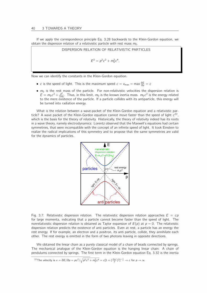
40 3 TOWARDS A THEORY
If we apply the correspondence principle Eq. 3.28 backwards to the Klein-Gordon equation, weobtain the dispersion relation of a relativistic particle with rest mass m0.
DISPERSION RELATION OF RELATIVISTIC PARTICLES
E2 = p2c2 +m20c
4,
Now we can identify the constants in the Klein-Gordon equation.
• c is the speed of light. This is the maximum speed c = vmax = max ∂E∂p = c
• m0 is the rest mass of the particle. For non-relativistic velocities the dispersion relation isE = m0c
2 + p2
2m0. Thus, in this limit, m0 is the known inertia mass. m0c
2 is the energy relatedto the mere existence of the particle. If a particle collides with its antiparticle, this energy willbe turned into radiation energy.
What is the relation between a wave-packet of the Klein-Gordon equation and a relativistic par-ticle? A wave packet of the Klein-Gordon equation cannot move faster than the speed of light c22,which is the basis for the theory of relativity. Historically, the theory of relativity indeed has its rootsin a wave theory, namely electrodynamics: Lorentz observed that the Maxwell’s equations had certainsymmetries, that were incompatible with the concept of an infinite speed of light. It took Einstein torealize the radical implications of this symmetry and to propose that the same symmetries are validfor the dynamics of particles.
p
anti particles
particles
E
light
: E=c
p light: E=−cp
m0c2
rest energy
nonrelativistic
dispersion relation
E=m0c2+p2/(2m0)
Fig. 3.7: Relativistic dispersion relation. The relativistic dispersion relation approaches E = cpfor large momenta, indicating that a particle cannot become faster than the speed of light. Thenonrelativistic dispersion relation is obtained as Taylor expansion of E(p) at p = 0. The relativisticdispersion relation predicts the existence of anti particles. Even at rest, a particle has an energy therest energy. If for example, an electron and a positron, its anti particle, collide, they annihilate eachother. The rest energy is emitted in the form of two photons leaving in opposite directions.
We obtained the linear chain as a purely classical model of a chain of beads connected by springs.The mechanical analogue of the Klein-Gordon equation is the hanging linear chain: A chain ofpendulums connected by springs. The first term in the Klein-Gordon equation Eq. 3.32 is the inertia
22The velocity is v = ∂E/∂p = pc2/√p2c2 +m2
0c4 = c[1 + (m0c
p)2]−
12 → c for p →∞

3 TOWARDS A THEORY 41
force of the individual beads. The second term is the force due to the springs between neighboringbeads. The last term can be described by a force between the displaced bead and its equilibriumposition.
Thus we have found a purely classical model, that describes a quantized relativistic particle. Thereis only one caveat: the displacements of the linear chain must be real, whereas the wave functionsbelonging to one branch of the dispersion relation are always complex.
3.7 Measurements
The purpose of any theory is to make predictions for measurable quantities. A measurable quantityis called an Observable. Examples for observables are energy, momentum, position etc. Howeverthere are also quantities that are not observable: The vector potential ~A(~r , t) of electrodynamics issuch an example: A gauge transformation yields different vector potentials, which describe exactlythe same physics. Thus the vector potential cannot be measured. Nevertheless, the magnetic field,which is directly related to the vector potential, can be measured.
In classical mechanics, the state of a system is described by the positions and momenta of allparticles. Thus all observables can be expressed as functions A(p, x) of positions and momenta.An example is the energy, which is expressed by the Hamilton function H(p, x) , or the angularmomentum defined as ~L(~r , ~p) = ~r × ~p.
Quantum mechanical wave packets, however, are spread over some volume. Therefore, they donot have a precise position nor a precise momentum. Thus, we need to perform an average in orderto attribute a value to an observable for a given wave packet.
We relate the square of the wave function to an intensity, just as in optics. On the other hand,the intensity has been related to the density of particles or the probability density to find a particleat a given point in time and space.
PHYSICAL MEANING OF THE WAVE FUNCTION
The absolute square φ∗(x)φ(x) of the wave function is interpreted as probability density for theparticle to be at a given position.
As a consequence of this probabilistic interpretation of the wave function, we need to requirethat a intensity of a wave function integrates to unity. We call this condition the normalizationcondition.
NORMALIZATION CONDITION
∫dx φ∗(x, t)φ(x, t) = 1 (3.33)
The normalization condition reflects that the probability for the system being in any state is equal toone.
Most of the previous discussion has been based on wave packets of the form φ(x, t) = χ(x, t)ei(kx−ωt),which are very localized on a macroscopic length scale, but delocalized on a length scale set by thewave length. Intuitively we identify the position 〈x〉 of a wave packet with the center of the intensity.
〈x〉 =
∫dx φ∗(x)xφ(x) =
∫dx |χ(x)|2x (3.34)
Thus we have defined what we mean with the position of a wave packet.Now let us turn to the momentum. The momentum of an extended wave packet should be related
to the wave vector k0 of the plane wave part.

42 3 TOWARDS A THEORY
The correspondence principle identified ~k with the momentum of a classical particle. We canobtain the momentum of a wave packet as
〈p〉 Eq. 3.28=
∫dx φ∗(x)
~i∂xφ(x)
Eq. 3.17= ~k − i~
∫dx χ∗(x)∂xχ(x)
= ~k −i~2
(∫dx χ∗(x)∂xχ(x) +
∫dx χ(x)∂xχ
∗(x)︸ ︷︷ ︸(A)
)
−i~2
(∫dx χ∗(x)∂xχ(x)−
∫dx χ(x)∂xχ
∗(x)︸ ︷︷ ︸(A)
)
= ~k −i~2
∫dx ∂x
(χ∗(x)χ(x)
)−m
∫dx
i~2m
(χ∗(x)∂xχ(x)− χ(x)∂xχ
∗(x))
︸ ︷︷ ︸Jχ(x)
= ~k −i~2
[χ∗(x)χ(x)
]∞−∞︸ ︷︷ ︸
=0
+~∫dx Im[χ∗(x)∂xχ(x)]
Im(χ)=0= ~k
The assumptions are that the envelope function is purely real, i.e. Im(χ) = 0, and that it vanishesat infinity.23
Thus we have defined what we mean with the momentum of a wave packet. We have used herethe Symbol 〈A〉 to denote the quantum mechanical mean value of an observable A consistent withthe expression Eq. 3.34 for the positions. Furthermore we required that the wave packet be localized,so that its amplitude vanishes at infinity.
Now, we need to generalize these results to more general observables A. In classical mechanics,an observable can always be expressed by a function A(x, p) of the positions and momenta. Thisis because positions and momenta characterize a classical state uniquely, two generalizations arepossible:
• we could attribute the observable to the function
〈A〉 = A(〈p〉, 〈x〉) (3.35)
of the mean values for positions and momenta obtained above.
• we could attribute the observable to the differential operator A( ~i ∂x , x) and evaluate the ex-pectation value as
〈A〉 =
∫dx φ∗(x)A(
~i∂x , x)φ(x) (3.36)
similar to the expressions for the positions and momenta.
Only the second choice, Eq. 3.36, is correct. Using the former choice, Eq. 3.35, a variable transformwould result in different expressions for the expectation value.
Another indication in favor of the second choice Eq. 3.36 is the following: The correspondenceprinciple, Eq. 3.28 on p. 38, provides us, together with the Schrödinger equation Eq. 3.29, with aprescription for the energy in the form:
〈E〉 Eqs. 3.28,3.36=
∫dx φ∗(x)i~∂tφ(x)
Eq. 3.29=
∫dx φ∗(x)H(
~i∂x , x)φ(x)
23The expression Jχ resembles the expression for the flux density. that is derived later in Section 8.4 on p. 131. Asit is applied only to the envelope function it has a different meaning in this case, and with the assumption of a realenvelope function the expression for Jχ vanishes altogether.

3 TOWARDS A THEORY 43
Since the energy H(p, q) is a perfectly allowed measurable quantity, our generalization must beconsistent with the expression given above. The alternative rule using 〈A〉 = A(〈p〉, 〈x〉) would givean inconsistent result.
Therefore, we set up the general rule for the evaluation of observables: start from a classicalobservable A(p, x, t) and replace momenta by its differential operator according to the correspondenceprinciple.
EXPECTATION VALUE OF A GENERAL OBSERVABLE
The expectation value of an observable, which is represented by a function of momenta and positionA(p, x), is obtained for a quantum mechanical system from its wave function as
〈A〉 =
∫dx φ∗(x)A( ~i ∂x , x, t)φ(x)∫
dx φ∗(x)φ(x)(3.37)
We have used here a form that does not require explicit normalization.
3.8 Postulates of Quantum mechanics
In this section, we have gone through the process of constructing a theory, that describes newexperimental facts from the double-slit experiment. We can now summarize our choices in a set ofpostulates.[4]
1. State: The state of a quantum mechanical system with one particle is fully described bythe wave function Ψ(~r , t), that depends on the position of the particle and the time. Forsystems with several particles, the wave function depends on the position s of all particles, i.e.Ψ(~r1, . . . , ~rN , t).
2. Dynamics: The time evolution of a wave function is determined by the Schrödinger equationEq. 3.29.
3. Observable: Observables are represented by linear differential operators acting on the wavefunction. We will see later that these differential operators need to have the property of beinghermitian, a term that will be described later.
4. Measurement: For a given state of the system only the probabilities for the outcome of anexperiment can be predicted. The mean value for the of the predicted outcomes is the ex-pectation value defined by Eq. 3.37. In particular, the expectation value of the observable Athat is defined by A(~r , ~p) = δ(~r −~r0) provides the probability density for finding the particle atposition ~r0. This probability density is the square of the wave function at position ~r0, that isψ∗(~r , t)ψ(~r , t).
This set of postulates is not formulated in its most general form. This set is also not complete anda few postulates for the measurement process will be added later.
The connection with classical mechanics is given by the following two requirements.
1. if the classical dynamics is governed by Hamilton equations with a Hamiltonian H(p, q), so that
E = H(~p, ~x)
the wave function evolves according the differential equation
i~∂tΨ(~r , t) = H(~i~∇, ~r)Ψ(~r , t)
The connection is provided by the correspondence principle Eq. 3.28.

44 3 TOWARDS A THEORY
2. If a classical observable is represented by a function A(~p, ~x), then the quantum mechanicaloperator representing the observable is obtained by the correspondence principle.
3. The transformation of a function into an operator via the correspondence principle is not alwaysunique. In those cases one has to choose that operator, which is hermitian.
3.9 Is Quantum theory a complete theory?
There is a fundamental question related to measurements, that is heavily discussed until today. Let usgo back to the diffraction pattern of photons. A theory based on waves, namely Maxwell’s equationscan describe the intensity of the electromagnetic field. However the experiment also shows that whenthe intensity is turned down, we observe a discrete signal here or there, but no more a continuoussignal.
There are two conclusions following out of this observation.
• The events come in chunks.
• The intensity corresponds to the probability of an event.
The second observation is the reason for calling the wave function the probability amplitude:φ∗(x)φ(x) is the probability to find the particle at position x .
The probabilistic nature of quantum mechanical predictions appears unsatisfactory, and seems toindicate that the theory is incomplete. The sentence “Gott würfelt nicht” (“God does not play dice”)was Einstein’s comment to quantum theory, but all attempts to find an inconsistency in the theory,or any contradiction between the predictions of the theory and experimental observation failed.
It is very difficult to imagine that any deterministic theory is capable of describing the outcomeof the double-slit experiment with an individual particle. The experimental setup we described for thedouble-slit experiment has been completely symmetric with respect to a mirror reflection about they = 0 line connecting the source with the midpoint of the two slits. The outcome of the individualsignals, however, is not symmetric. A single particle can appear anywhere, as long as the probabilityis finite, which in general is off-center and therefore not symmetric, unlike the experimental setup.Hence we cannot use a symmetric theory to predict the outcome for a single particle. We need amechanism to break the symmetry. But where do we take the information how the symmetry isbroken? Until we find some uncontrolled environmental effects not considered in the experimentalsetup as we described it, we need to be content with the probabilistic theory.
Do we have to accept a theory that is less complete and predictive than classical mechanics? Notreally: think of chaos. If we would know the exact values of positions and velocities of a particle andthe equations of motion, classical mechanics can, in principle, predict the outcome for all future. Butis the exact specification of the initial conditions meaningful? Try to devise an experiment so thatthe trajectory is prepared in a unique way far into the future. It does not suffice to determine theinitial conditions very, very accurate. Accurate is not what we mean with exact. After some time,trajectories in a chaotic system with even slightly different initial conditions deviate completely fromeach other. Hence, also in classical mechanics there are experiments, whose outcome we cannotpredict with arbitrary certainty.
On the other hand, there are experiments for which quantum mechanics provides exact predictions.Namely those for which the probability distribution shrinks to a point.
When we compare quantum mechanics and classical mechanics closely, the difference in thecompleteness appears more gradual than qualitative.

3 TOWARDS A THEORY 45
3.10 Planck constant
We still need to determine the value of one undetermined constant, namely the Planck constanth. In practice, the reduced Planck constant ~ def
= h2π is used24 and often both are named in the
same way, namely as Planck constant. Sofar the Planck constant played the role of an arbitraryproportionality constant in the correspondence principle E = ~ω, p = ~k .
Only experiment can tell us the value of ~. The best value of ~ is currently[19, 20]
~ = 1.05457168× 10⁻³⁴kgm2
s(3.38)
What is the physical meaning of ~?
• The unit of ~ is that of an angular momentum ~L = ~r × ~p or of a phase-space-volume elementdp dx .
• Planck constant determines the length scale on which the wavy nature becomes evident, namelythe wave length λ. Given a classical particle with velocity v , the wave length is λ = 2π
k = 2π~p =
2π~mv . We recognize that the wavelength vanishes if Planck constant would be zero. In this case,we would return to classical physics, where the oscillations are so rapid that they cannot beobserved.
• The limit of fast particles is similar to the classical limit ~ → 0. Indeed, quantum mechanicaleffects seem to become unimportant at high temperatures.
• Let us consider a few real world examples:
– What is the wave length of a walking person? Let us make an estimate: the person shouldweigh 72 kg and walk with a speed of 3.6 km/h=1m/sec. Its wave length is thereforeλ ≈ 10−35 m. This is the 1025th fraction of an interatomic distance. Thus we can safelydescribe a person by classical physics.
– The situation is different for an electron. An electron has a mass of about 10−30 kg. Thewave length of an electron at the same speed is already three millimeter or about 107
atomic distances.
3.11 Wavy waves are chunky waves: second quantization
We have mentioned that we have an intensity which we identify with a particle number. However,sofar we have no way to explain why the intensity comes in chunks, as we expect it from particles.Here I will give a brief outlook on how the chunks are explained. I cannot give here the theory in itsfull glory, because that fills another lecture series on its own. Rather I want to sketch the main linesof thought.
Our starting point was the linear chain. We built it up from particles connected by springs. Amodification of the linear chain revealed, that the collective motion of the beads produces wavepackets, that behave like classical particles. Hence we identified particles with wave packets. Tobe consistent, we have to describe also every bead of the chain by a wave packet. What are theconsequences?
Let us consider a violin chord as a realization of the continuous linear chain.25 The violin chord24The Planck constant is defined as h. This has been a somewhat unfortunate choice, because h appears nearly
always in combination with 1/(2π). Therefore, the new symbol ~ = h/(2π), denoted reduced Planck constant hasbeen introduced. The value of ~ is ≈ 10−34 Js to within 6%.
25The linear chain is not exactly the correct model for a violin chord. The transversal oscillation of the violin chorddiffers from the longitudinal oscillation of the linear chain. However, for small displacements the transversal oscillationbehaves mathematically similar to a longitudinal oscillation. A better realization of the linear chain would be a rubberchord stretched along its direction.

46 3 TOWARDS A THEORY
produces waves that are enclosed by its end points. A violin chord oscillate with frequencies that aremultiples of the pitch. It does not oscillate with any other frequencies.
What the violin chord is for a massless particle, the harmonic oscillator is for a massive particle.Remember, that we identified the linear chain with a massless particle. The wave function of aparticle with mass in a harmonic potential oscillates with frequencies that are multiples of the classicaleigenfrequency (plus a constant). The frequency is related to the energy. Thus the energy of sucha system can change in discrete steps.
Let us consider a chain where we freeze all beads except one. This bead can be described by aharmonic oscillator. Its energy is discretized, like the frequency of a violin chord. Thus we have aspecial wave, which comes in chunks. Each frequency corresponds to a given number of particles.Since the energy of a wave is always quadratic in the wave function amplitudes, it can always be relatedto harmonic oscillators and all harmonic oscillators have discrete and equidistant energy levels. Hence,when the wave function amplitude (or the position of the beads) is described by wave packets, allfield theories of the type discussed so far result in chunky waves.
Thus we have an additional dimension in addition to space and time, namely the field of a givenparticle. This system is described by a wave function φ(x, t). If we quantize this world, we obtainchunky fields and particle waves.
3.12 Summary
In this section we introduced the Schrödinger equation. In three dimensions the Schrödinger equationhas the form:
i~∂tψ(~r , t) = H(~i~∇, ~r)ψ(~r , t) (3.39)
It has been obtained from the classical energy expression E = H(~p,~r) which is transformed into adifferential equation by using the correspondence principle, E → i~∂t and ~p → ~
i~∇, and multiplication
by the wave function.
• ψ(~r , t) is the wave function. ψ is a complex function and the absolute square value P (~r , t) =ψ∗(~r , t)ψ(~r , t) is the probability density to find the particle at point ~r in space at time t.
• the Hamilton operator H( ~i~∇, ~r) is obtained from the Hamilton H(~p,~r) function by replacing
the momentum ~p by the momentum operator
~p =~i~∇ (3.40)
• ~ = 1.054 × 10⁻³⁴ Js is Planck’s constant (germ: Planck’sches Wirkungsquantum). Notethat h = 2π~ is called by the same name. If Planck’s constant were zero, we would obtain ourtraditional classical point mechanics.
Instead of describing a particle as a point with defined position and a momentum, in quantummechanics we describe particles by a wave packet with a intensity distribution φ∗(x)φ(x) and amomentum distribution.
The wavy nature of the wave packets becomes evident only at small length scales, so that itevaded observation for a long time. One exception is again electromagnetism. There the wavelength can be very large. Here a field theory has been used a long time before quantum mechanicshas been invented.
We have also sketched how the quantization of the wave function itself naturally leads to theconcepts of chunks of the wave, which are identified as individual particles. Thus we changed ourperspective radically, from point-like particles to “waves of waves”. The macroscopic predictions ofquantum theory are, however, still in accord with the particle picture classical mechanics.

Chapter 4
Quantum effects
Fig. 4.1: Max Planck, 1858-1947. German Physicist. No-bel price 1918 for the discov-ery of energy quanta. Photoaus dem Jahr 1901
In this section, we will explore the physical effects that result fromthe Schrödinger equation:
QUANTUM EFFECTS
• Spreading of wave packets,
• Splitting of wave packets,
• Tunnel effect,
• Quantized energy levels,
• Zero-point energy, and
• Resonances.
One of the main tasks of this section is to become familiar withthe similarities and differences of quantum-mechanical particle waveson one side and either classical particles or classical waves on theother side. The comparison will lead us to conceptual difficulties thatwe have to become familiar with. The reason we try to compare toclassical problems is that this allows us to use the experience thatwe have already gained. However, it is important to also gain athorough understanding of the conceptual problems.
In order to illustrate the quantum effects, I am choosing a class of very simple problems thatcan be solved analytically, namely systems where the potential varies only in one dimension andis piecewise constant. Thus the particles behave like free particles except where the value of thepotential changes abruptly to another value. The problems are
• the free particle,
• the potential step,
• the particle in a box,
• the potential barrier, and
• the potential well.
47

48 4 QUANTUM EFFECTS
4.1 Quasi-one-dimensional problems in the real world
Even though the examples are chosen to introduce quantum effects, the one-dimensional problemsdiscussed in the following play an important role in practical problems. All these problems can berealized and have been used in electronic devices.
Electronic devices are build by bringing different materials into contact with each other, in order tocontrol the flow of electrons through these devices. Three basic types of materials play a role: metals,which conduct electrons freely, insulators which do not conduct electrons, and semiconductors whichcan be made conducting or insulating depending on the electrostatic fields, temperature and doping.
E
E
EF
p
EF
p
Eg
Ec
Ev
Fig. 4.2: Schematic bandstructure of a metal (top)and an insulator (bottom).EF is the Fermi level. Eg isthe band gap of the insula-tor. Ev is the top of thevalence band and Ec is thebottom of the conductionband.
Each material can be considered to be homogeneous and each ma-terial has its own dispersion relation for the electrons. This dispersionrelation is called band structure1. Every state can be occupied by amaximum of two electrons. The bands, the branches in the dispersionrelation, are filled with electrons up to an energy, the so-called Fermienergy EF . In Fig. 4.2 we divide materials into two classes: If a bandcrosses the Fermi energy the material is a metal. Otherwise it is aninsulator or a semiconductor. In this case, a forbidden energy region,where electrons cannot travel, separate the filled states, called the va-lence bands2, from the empty states, called the conduction bands.The forbidden energy region is called the band gap.
If there is no electric field, there are as many electrons moving rightas there are electrons moving left. As a consequence there is no netelectric current. An electrical current flows only when the balance ofelectrons moving into opposite directions is broken, which can only hap-pen when electrons are excited above the Fermi energy. In a metal thereis no minimum energy to excite electrons. Therefore, metals conductelectrons at all temperatures. In an insulator, the band gap is so largethat thermal energies are insufficient to lift electrons from the valenceband into the conduction band. Therefore, hardly any current flows inan insulator. In a semiconductor, the band gap is sufficiently small, sothat the conductance can be easily modulated by temperature, dopantatoms and external fields.
We can learn a lot about electrons in materials from the free particlemodel, which underlies much of the discussion in this chapter. In asemiconductor, only the lowest part of the conduction band and theuppermost part of the valence band matter for electron transport, because thermal energies are smalland cannot lift many electrons much higher. Therefore, we can perform a Taylor expansion of theconduction band about the minimum up to second order. This gives a parabola shaped dispersionrelation, which can be written as
E(k) = Ec +~2~k2
2m∗c
Ec is the conduction band minimum and m∗c is called the effective mass of the conduction electron.Similarly we can describe the hole by a dispersion relation
E(k) = Ev −~2~k2
2m∗v
where Ev is the valence band top and m∗v is the effective mass of the holes. Holes behave as particleswith a positive charge, similar to positrons.
1The concept of band structures is more general. There are band structures for phonons, that are the quantaof lattice vibrations. There are even band structures for photons in so-called photonic crystals, a recent and highlyinteresting research area.
2Usually one distinguishes the valence states from so-called core states, which are also occupied. Core states arelocated so close to the nucleus, that they do not interact with neighboring atoms.

4 QUANTUM EFFECTS 49
We have seen that particles which interact with a material behave like free particles but withchanged properties such as the mass or the charge. Such particles are called quasiparticles. Thesituation is similar to that of light entering a material. Inside the material the speed of light is lowerthan in vacuum, which explains the refractive index of materials. Also here we consider the photonand the response of the material to the electric fields of the photon as one quasi particle.
We have done some simplifications: In reality (1) the effective mass can be a 3 × 3 tensor. (2)The minimum need not to be located at k = 0. (3) There may be several minima and several nearbybranches of the bands at the conduction and valence band edges.
In a metal, the band structure can be described by a parabola with a minimum below the Fermienergy. Only electrons near the Fermi energy contribute to the current. Close to the Fermi energy,the dispersion relation is approximately linear with the wave vector ~k , so that the electrons have aconstant velocity similar to light and sound waves.
Here I will describe the realization of the model systems discussed in this section in electronicdevices:
• The free particle describes for example the transport in a bulk material
• The potential step is a model for an interface between two materials with different band edges.
• In the particle in the box a particle is confined in all three spatial directions as in a quantumdot. A quantum dot could be realized by surrounding a semiconductor by an insulator, sothat any conduction electrons cannot escape. Quantum dots are used for example for so-calledsingle electron transistors. If the particle is confined only in one direction, the particle in the boxdescribes a two-dimensional electron gas, which was important to obtain the so-called quantumHall effect, for which v. Klitzing was awarded the Nobel prize.
• The finite barrier is realized by an insulating layer between two metals or semiconductors.The finite barrier is a model of a gate oxide in a MOSFET3 transistor to describe its tunnelcurrent. Also the scanning tunneling microscope (Nobel prize H. Rohrer and G. Binnig) usesthe tunneling current from a surface to a tip to monitor surfaces with atomic resolution.
• A particle in a well describes electrons in a structure that can be made by depositing twodifferent semiconductors A and B in the sequence ABA. Since the conduction band edge ofthe semiconductor B is higher or lower than that of A, the conduction band edge forms eithera finite barrier or a finite well. The transport through a finite well is relevant for the transportthrough a “resonant tunnel diode”
3MOSFET=Metal-oxide-semiconductor field-effect transistor

50 4 QUANTUM EFFECTS
• Dirac atom (not yet included) The Dirac atom is the most simple one-dimensional model foran atom. It is a model for a two-dimensional electron gas or a one-dimensional conductor.
Almost any of these quasi-one-dimensional problems can be realized by growing thin layers ofsemiconductors onto other semiconductors. Such structures can be very complex and are calledmultilayer structures.
4.2 Time-independent Schrödinger equation
Before we enter the discussion of quantum effects, we need to become familiar with the time-independent Schrödinger equation. If the Hamiltonian is time independent, the Schrödinger equationcan be substantially simplified. Time-independent problems are so abundant, so that most of ourdiscussion will address those problems.
For time-independent problems, the wave function can be broken up into a product of a time-dependent part, and a time independent part, which depends only on the atomic position. Thetime-dependent part is trivial. The time-independent part of the wave function obeys the time-independent Schrödinger equation.
Let us Fourier transform the Schrödinger equation with respect to the time.4 The time-dependentwave function ψ(r, t) is related to its Fourier-transformed counterpart ψ(r, ~ω) by5
ψ(~r , t) =
∫dω
2πe−iωtψ(~r , ~ω) (4.1)
Inserting the Fourier transform into the Schrödinger equation Eq. 3.29 yields6(i~∂t −H(
~i~∇, ~r)
)Ψ(r, t) = 0
Eq. 4.1⇒(i~∂t −H(
~i~∇, ~r)
)[∫dω
2πe−iωtψ(~r , ~ω)
]= 0
⇒[∫
dω
2π
(i~∂t −H(
~i~∇, ~r)
)e−iωtψ(~r , ~ω)
]= 0
⇒∫dω
2πe−iωt
[(~ω −H(
~i~∇, ~r)
)ψ(~r , ~ω)
]︸ ︷︷ ︸equation holds only if this vanishes
= 0
4Note here that we denote the Fourier transform with the same symbol as the original functions. Mathematicallythis is incorrect! However, this notation is very convenient when used cautiously. When we evaluate the function valuewe need not only the numeric value of the argument, but also the type. So if we evaluate the function for a giventime, we obtain a different result than if we evaluate the function for a frequency with the same numeric value. Wewill later see how such a notation can be formulated rigorously in the bracket formalism of Dirac.
5The reader may be wonder why we use e−iωt instead of eiωt , which would be our regular notation of a Fouriertransform. The origin of te minus sign is that we derived the Schrödinger equation from plane waves ei(kx−ωt). Thesign convention for ω is a matter of choice, but if we use this form of the Schrödinger equation, we need to adhere tothis choice.
6Plane waves eiωt are linear independent. Linear independency implies that no superposition∑i cie
iωi t of different(ωi 6= ωj ) plane waves can result in a vanishing function. Thus the expression∫
dω
2πc(ω)eiωt = 0
can hold for all t only, when c(ω) = 0. Because plane waves are linear independent, the Fourier transform is unique.

4 QUANTUM EFFECTS 51
We obtain
H(~i~∇, ~r)ψ(~r , ~ω) = ψ(~r , ~ω)~ω
after realizing that the equation must be valid for every Fourier component.By replacing ~ω with E, we obtain the time-independent Schrödinger equation.
TIME-INDEPENDENT SCHRÖDINGER EQUATION
H(~r ,~i~∇) ψ(~r , E) = ψ(~r , E) E (4.2)
We call such an equation an eigenvalue equation. The equation has solutions only for specificvalues of E. These values are the eigenvalues of the Hamiltonian. The set of all eigenvalues iscalled the spectrum. The solution ψ(~r , E) is called an eigenstate of the Hamiltonian.
An eigenvalue equation is similar to the problem of diagonalizing a matrix, A~cn = ~cnλn. Theonly difference is that the differential operator is replaced by a matrix and the vector is replacedby a function in space. We will see later that this difference is smaller than one might think. Thedifference is related only to the fact that in one case we describe finite matrices and vectors and inthe other case infinite vectors and matrices. We will return to this aspect in detail in chapter 5.
There may be several solutions to a given energy. We call such solutions degenerate. Thetime-independent Schrödinger equation may have solutions for discrete values for the energy E, orfor continuous sections of the energy axis. The set of allowed energy values is called the eigenvaluespectrum of the Hamilton operator. The energy spectrum of the Hamilton operator is bound frombelow, which is exploited in the variational principle described in Section 13.5.
Once we know all eigenstates ψσ(~r , E), of the time-independent Schrödinger equation, we candetermine the wave function for all times as
ψ(~r , t)Eq. 4.1
=
∫dE
2π~e−iEt/~
∑σ
ψσ(~r , E)aσ(E)
We use the index σ to distinguish different eigenfunctions for the same eigenvalue.The initial conditions, represented by the values ψ(r, t = 0), determine the coefficients aσ(E) of
this expansion in stationary states.
ψ(r, t = 0) =
∫dE
2π~∑σ
ψσ(r, E)aσ(E)
4.3 Method of separation of variables
In this chapter we will work almost exclusively with one-dimensional problems. One may ask howmuch this has to do with the real three-dimensional world? The answer is given by the method ofseparation of variables.
As in classical mechanics, it is often possible to exploit symmetries to break down a problem intoproblems of lower dimensions, and, if we are lucky, into one-dimensional problems. An example is aproblem with a potential that varies only in one dimension, so that it is translationally invariant inthe other directions.
Quasi-onedimensional problem in three dimensions
Let us try to exploit this symmetry on a quasi-onedimensional problem: consider the Schrödingerequation with a potential that varies only in x-direction:
i~∂tΨ(~r , t) =[−~2
2m∇2 + V (x)
]Ψ(~r , t) (4.3)

52 4 QUANTUM EFFECTS
We can write the Hamiltonian Eq. 4.3 as sum H = H1 + H2 + H3 of three terms, where each actson one variable
H1 =−~2
2m∂2x + V (x); H2 =
−~2
2m∂2y ; H3 =
−~2
2m∂2z
We make a product ansatz for the wave function
Ψ(~r , t) = φ1(x, t)φ2(y , t)φ3(z, t) (4.4)
where each term φi solves the corresponding one-dimensional Schrödinger equation.
i~∂tφ1(x, t) =
[−~2
2m∂2x + V (x)
]φ1(x, t)
i~∂tφ2(y , t) =−~2
2m∂2yφ2(y , t)
i~∂tφ3(z, t) =−~2
2m∂2zφ3(z, t) (4.5)
In order to show that this ansatz yields the correct result, we insert it into the Schrödinger equationEq. 4.3. We divide the equation by the wave function, which allows us to write the equations in amore economical fashion.
1
Ψ(~r , t)i~∂tΨ(~r , t)
product rule=
i~∂tφ1(x, t)
φ1(x, t)+i~∂tφ2(y , t)
φ2(y , t)+i~∂tφ3(z, t)
φ3(z, t)
Eq. 4.5=
1
φ1(x, t)
[−~2
2m∂2x + V (x)
]φ1(x, t)
+1
φ2(y , t)
[−~2
2m∂2y
]φ2(y , t) +
1
φ3(z, t)
[−~2
2m∂2z
]φ3(z, t)
Now there is the only tricky part: We can multiply the first term on the right-hand side with φ2φ3
from the right side and divide by the same on the left hand side. This does not change the result,because the Hamiltonian H1 does not act on φ2φ3. Similarly, we multiply the second term with φ1φ3
on the right and divide by the same factor on the left. Finally, we multiply the second term withφ1φ2 on the right and divide by the same factor on the left.
Thus we obtain
1
Ψ(~r , t)i~∂tΨ(~r , t) =
1
Ψ(~r , t)
[−~2
2m∂2x + V (x)
]Ψ(~r , t)
+1
Ψ(~r , t)
[−~2
2m∂2y
]Ψ(~r , t) +
1
Ψ(~r , t)
[−~2
2m∂2z
]Ψ(~r , t)
⇒ i~∂tΨ(~r , t) =
[−~2
2m∂2x + V (x) +
−~2
2m∂2y +−~2
2m∂2z
]Ψ(~r , t) = HΨ(~r , t)
This proves that our ansatz, Eq. 4.4 with Eq. 4.5, yields the correct solution.
General case
The method of separation of variables is not limited to quasi-one-dimensional problems. It can beapplied to a whole class of Hamiltonians. Let us state it in some greater generality.

4 QUANTUM EFFECTS 53
METHOD OF SEPARATION OF VARIABLES
If the Hamiltonian is a sum of several parts, where each part only acts on one variable such as
i~∂tΨ(x1, x2, . . . , t) =
∑j
Hj(~i∂j , xj , t)
Ψ(x1, x2, . . . , t) (4.6)
then the wave function can be expressed as
Ψ(x1, x2, . . . , t) =∏j
φj(xi , t) (4.7)
with
i~∂tφj(x, t) = Hj(~i∂j , x, t)φj(x, t) (4.8)
Thus we have broken down the multidimensional problem into many one-dimensional problems, thatare much easier to solve. Of course, due to the superposition principle, any superposition of suchsolutions is again a solution.
In the proof, we exploit that the Hamilton operator Hi( ~i ∂i , xi , t) does not act on wave functionsφj(xj , t) with j 6= i . They do not depend on the parameter xi on which the Hamilton operatorHi(
~i ∂i , xi , t) acts. Therefore, Hi( ~i ∂i , xi , t)φj(xj , t) = φj(xj , t)Hi(
~i ∂i , xi , t) for j 6= i .
The proof of Eq. 4.6 with Eqs. 4.7,4.8 goes as follows
i~∂t∏i
φi(xi , t)︸ ︷︷ ︸Ψ(~r ,t)
product rule= [i~∂tφ1(xi , t)]φ2(x2, t) · · ·+ φ1(x1, t) [i~∂tφ2(x2, t)] · · ·+ . . .
=
[∏i
φi(xi , t)
]∑i
1
φi(xi , t)i~∂tφi(xi , t)
Eq. 4.8=
[∏i
φi(xi , t)
]∑i
1
φi(xi , t)Hi(~i∂i , xi , t)φi(xi , t)
=∑i
Hi(~i∂i , xi , t)
[∏i
φi(xi , t)
]︸ ︷︷ ︸
Ψ(~r ,t)
q.e.d.
The method of separation of variables can be used, if we are able to express the Hamilton operatorby a sum of differential operators that only depend on a single variable. Sometimes the choice is notimmediately apparent and a coordinate transform is required to bring it into the desired form. Themethods of finding such variable transforms are similar to the techniques used in classical mechanics,such as the transformation on center-of-mass and relative coordinates in a many particle system andthe division into angular and radial coordinates in a spherical system.
Most Hamiltonians, however, cannot be written in this simple form. Even if the problem cannotbe separated exactly, the method of separation of variables is invaluable in finding approximate so-lutions. As most quantum mechanical problems cannot be solved analytically or even numerically, itis important to find models that represent the true system closely – even though not exactly –, butcontain symmetries that allow to break down the problem. This approximate model is the startingpoint for approximation techniques discussed in section 13 to include whatever has been neglected inthe model system.

54 4 QUANTUM EFFECTS
4.4 Free particles and spreading wave packets
A free particle does not experience forces. It experiences a constant potential. Thus, it obeys theSchrödinger equation [−~2
2m∂2x + V0
]ψ(x, E) = Eψ(x, E) (4.9)
with a spatially constant potential V (x) = V0.The solutions can be found using the Ansatz ψ(x, E) = eikx . By insertion we find the dispersion
relation
E(k) =~2k2
2m+ V0
The energy eigenstates of a free particle are plane waves
Ψ(x, E) = eik(E)x (4.10)
with a wave vector k that has length k(E) = ± 1~√
2m(E − V0).We have discarded the solutions with E < V0. They are not plane waves, but exponential
functions. Neither plane waves nor exponential functions are normalizable. Therefore, they cannotdescribe the wave function of a single particle. While for the plane waves, a way out of this dilemmahas been found, for the exponential function the problem cannot be cured. Nevertheless, exponentialsolutions will play a role as partial solution in problems that have been pieced together.
A few properties are noteworthy:
• The intensity φ∗(x)φ(x) = e−ikxeikx = 1 of the plane wave is uniformly distributed over allspace.
• The momentum of a plane wave is 〈p〉 =∫dxψ∗(x) ~
i∂xψ(x)∫
dxψ∗(r)ψ(r)= ~k . Furthermore, the spread of
momenta 〈(p − 〈p〉)2〉 = 〈p2〉 − 〈p〉2 vanishes for a plane wave.
Thus a plane wave describes a beam of particles flying with the same momentum p, or in other words,constant velocity v = ∂pE(p) = p
m .
Free particle in three dimensions
We can use the result for the free particle in one dimension and the method of separation of variablesto obtain a solution for a free particle in three dimensions: The wave function in three dimensions isthe product of the three one-dimensional free particles.
Ψ(~r) = eikxxeiky yeikzz = ei~k~r
Here it becomes apparent why we denote ~k as wave vector.The energy is the sum of the three one-dimensional problems
E(~k) =(~~k)2
2m+ V0
and the momentum is
〈~p〉 Eqs. 3.28,3.37=
∫d3r Ψ∗(~r) ~i
~∇Ψ(~r)∫d3r Ψ∗(~r)Ψ(~r)
= ~~k
The velocity7 of the particles in the beam is then ~vEq. 3.6
= ~∇E(~p) = 1m ~p.
7The group velocity of a wave packet has been linked to the dispersion relation ω(k). The Schrödinger equation hasbeen constructed such that its dispersion relation is analogous to that of classical particles E = H(p, x, t). Therefore,we may use Hamilton’s equations, that in principle are equations of motion for classical particles.
4 QUANTUM EFFECTS 55
Wave functions that are not normalizable
There is a problem related to solution Eq. 4.10: It cannot be normalized, because the integral Eq. 3.33is infinite. This would contradict the interpretation of the wave function as probability amplitude.
There are two possible ways around the problem.
1. Instead of an infinite integration volume we consider a large but finite volume, such as theuniverse, which in fact is finite. In the finite volume the wave function is normalizable. Further-more, the spectrum in a finite volume is discrete, and does not contain continuous sections.The disadvantage is that the amplitude of the wave function is extremely tiny, if the volume isvery large. This point of view, which we will adopt in most of this book, avoids mathematicalsubtleties. Before the expressions are evaluated in practice, one has to take the limit of infinitevolume.
2. We consider the non-normalizable wave function only as one part of the true wave function.The true wave function would be a product of the non-normalizable wave function with anenvelope function that itself is normalizable, such as the wave packet
ψ(~r , t) = χ(~r , t)ei(~k~r−ωt)
where the plane wave is not normalizable, but the envelope function χ(x, t) is normalized. Bymultiplication with a normalizable envelope function, the complete wave function is normal-izable. The corresponding energy eigenvalue spectrum may contain discrete eigenvalues and,simultaneously, energy regions with a continuous set of eigenvalues.
The second choice is the mathematically more sophisticated approach. In a way, it limits the in-tegration volume like the first suggestion. It does it in a way so that the wave function remainsdifferentiable everywhere in space.
4.4.1 Wave packets delocalize with time
Let us explore, what happens with a free particle that is localized in space. We start with a wavepacket of Gaussian shape8. We use the ansatz
ψ(x, t) = A(t)e−12B(t)x2
, (4.11)
which leads to differential equations for A(t) and B(t). Because the derivation is a bit lengthy, wesolve the problem in the App. B. Here, we only report the solution:
ψ(x, t)Eq. B.16
= 4
√C0
π|C(t)|2 e−1
2C(t)x2
with C(t)Eq. B.11
= C0 +i~tm
(4.12)
The symbol C0 is the initial value of C(t). The wavefunction acquires a complex phase, becauseC(t) becomes complex. As a result the wave function oscillates in space.
What we are mostly interested in is the probability to find the particle at a certain point in space.Let us therefore evaluate the probability distribution P (x) = ψ∗(x, t)ψ(x, t).The derivation is foundagain in appendix B. Here we only report the result.
P (x)Eq. B.17
=1√
2π · d(t)e− 1
2
(xd(t)
)2
with d(t)Eq. B.18
= d(0)
√1 +
(~t
2md2(0)
)2
(4.13)
The initial width is related to the coefficient C in Eq. B.11 by d(0) = 12
√C0. The density maintains
its Gaussian shape, but the width, which is proportional to d(t) grows, after a certain while, almostlinearly with time, that is d(t)→ ~t
2md(0) for t →∞.
8A Gaussian has the form e−ax2.

56 4 QUANTUM EFFECTS
t0
d(t)
Fig. 4.3: Decay of a Gaussian wave packet with time. The horizontal axis is a spatial coordinate.The full line is the real part of the wave function and the dashed line is the imaginary part. Thethree figure represent the initial state and equi-distant later times. Note that the absolute squareof the wave packet maintains its Gaussian shape. Real and imaginary part however oscillate. Theoscillation is more rapid in the wings: The wings are made of the contributions that run away mostquickly, which also have the smallest wavelength.(vg = 1
m~k).
Something strange happens here: the smaller the wave packet is initially, the faster it spreadsout. In other words, a small width d(0) leads to a rapid growth of the width as seen from Eq. 4.13.This observation can be rationalized as follows: When we build a narrow Gaussian from plane waves,
1√2π · d
e−12 ( x
d )2
=
∫dk
2πeikx e−
12
(d ·k)2
, (4.14)
we have to include plane waves eikx with large kinetic energy ~ω(k). Those contributions have highvelocity and run away quickly.
What we see here, is another manifestation of Heisenberg’s uncertainty relation , which willbe derived later in section 7.4. Heisenberg’s uncertainty relation says that if the position of a particleis well known, there is a large uncertainty about its momentum. In other words, if the position isprecisely determined, that is if the width of the wave packet is small, the spread in velocities is large.
Delocalization in practice
Let us consider a person who has a mass of 50 kg and let us consider that its position is initiallycertain to within the thickness of a hair that is d(0) = 1 µm. How long does it take until the
position becomes uncertain to about d(t) = 1 mm. With ~ ≈ 10−34kg m2/s, we obtain tEq. 4.13
=1~2md(0)d(t) = 1027 s. Because a year has about 3× 10⁷ s, we have to wait 1020 years!
On the other hand, let us consider a microscopic particle such as an electron: The electron hasa mass of about 10−32 kg. To spread from 1 µm to 1 mm, takes only one tenth of a microsecond.
Now let us consider a truly microscopic situation: Let us localize an electron on a single atom,which has a radius of about 0.1 nm=10−10 m. What is the localization region after a typical atomic

4 QUANTUM EFFECTS 57
oscillation period of about 10−13 s? Its diameter has grown to a few µm or 10,000 times the sizeof an atom. This indicates that the atoms do not experience the electrons as “particles” but asdelocalized waves.
This discussion explains why delocalization as quantum effect is not observable in our daily life,while it is essential in the nano-world.
4.4.2 Wick rotation
The decaying wave packet reminds us of a diffusion process. While the process of a diffusing particleis entirely different from that of a spreading wave packet, there is an intrinsic connection on amathematical level. The diffusion equation is closely related to the Schrödinger equation. Considerthe diffusion equation
∂tρ(~r , t) = D~∇2ρ(~r , t)
where ρ is the density and D is the isotropic diffusion constant. Now let us perform the so-calledWick-rotation
D →~2
2mand t →
i t
~and ρ→ ψ
then we obtain from the diffusion equation the Schrödinger equation of a free particle.
i~∂tψ(~r , t) = −~
2m~∇2ψ(~r , t)
The close connection between quantum mechanics and statistical mechanics, which has becomeevident here, has been extremely fruitful in the past and has lead to the Quantum Monte Carlomethod and the Renormalization theory for the description of phase transitions (Kenneth G. Wilson,Nobel prize for Physics 1982).
4.4.3 Galilei invariance (home study)
We have seen that the wave function of a resting wave packet spreads equally in all directions. Theanalogy with the diffusion equations may lead to a misunderstanding that this is also true if theparticle have initially a non-zero mean velocity. Such a behavior would violate Galilei invariance,saying that the laws of nature are independent of the velocity of an observer. This is the reason forinvestigating a wave function with a finite velocity and its relation to the resting wave packet.
Galilei invariance implies that the laws of nature are independent of a (constant) velocity of theobserver. In other words, there is no absolute velocity.9 Here we illustrate, rather than prove, Galileoinvariance of the Schrödinger equation for a free particle by investigating how a wave packet changesits shape with time.
We will see that envelope function of a free particle does not remain constant with time: Firstly,it moves with a velocity v = dE
dp and secondly it changes its shape slowly so that eventually it coversall space. We will show that a moving wave packet behaves exactly the same way as a resting one.
In order to show this equivalence between a moving wave packet and a resting one, we proposea transformation from a resting wave packet to one moving with velocity v . Then we show that thetransformed wave packet obeys the Schrödinger equation if the resting does as well.
If Ψ0(x, t), the “resting wave packet”, obeys the Schrödinger equation for a free particle, thenalso the wave function
Ψv (x, t)def= Ψ0(x − vt, t)ei(kx−ω(k)t) , (4.15)
9Note that the problem with an external, spatially dependent, potential V (x) is not Galileo invariant, because thatpotential is fixed in space. However, if we step back and include whatever creates that potential into the description.This enlarged system is Galileo invariant.

58 4 QUANTUM EFFECTS
the “moving wave packet,does”, if v is the group velocity
v = ∂kω
Interesting is that the transformation does not only correspond to a time dependent shift of the wavefunction, but that it obtains in addition a phase factor, the plane wave. A more detailed derivationis given in appendix A on p.251.
Now we show by insertion that the moving wave packet Ψv (x, t) as defined in Eq. 4.15 obeys theSchrödinger equation.
0?=[i~d
dt−−~2
2m∂2x
]Ψ0(x − vt︸ ︷︷ ︸
def=y(x,t)
, t︸︷︷︸def=τ(x,t)
)ei [kx−ωt]
= ei [kx−ωt][−i~v∂y + i~∂τ + ~ω +
~2
2m(∂2y + 2ik∂y − k2)
]Ψ0(y(x, t), τ(x, t))
= ei [kx−ωt][i~∂τ +
~2
2m∂2y − (v −
~km
)︸ ︷︷ ︸=0
i~∂y + (~ω −~2
2mk2)︸ ︷︷ ︸
=0
]Ψ0(y , τ)
= ei [kx−ωt][i~∂τ −
−~2
2m∂2y
]Ψ0(y , τ)︸ ︷︷ ︸
=0
= 0 (4.16)
Thus, we have shown that Ψv (x, t), as defined in Eq. 4.15, is a solution to the Schrödinger equationfor a free particle, if
• k = 1~mv ,
• ω = 1~~2k2
2m = 1~
12mv
2 and, if
• Ψ0 obeys the Schrödinger equation for a free particle as well.
Note that the total derivative d/dt acts also on the argument y(x, t) = x − vt, whereas thepartial derivative only acts on the second argument of χ. In the last step we simplified using thedispersion relation and v = ∂ω
∂k = ~km
Eq. 4.16 is nothing but the Schrödinger equation for a particle at rest. Thus the shape of theenvelope function is independent of the velocity of the wave packet. This is Galileo invariance: Theequations of motion do not depend on the relative velocity between the object and the observer.
4.5 Particle in a box, quantized energies and zero-point motion
The particle in a box is our simple model for an atom. In a hydrogen atom, the electron is bound to thenucleus by electrostatic attraction. Under normal circumstances, the electron cannot overcome thisattraction. We simplify the problem by replacing the Coulomb potential of the nucleus by a constantinside the attraction region and infinitely high potential walls, which ensures that the electron doesnot get lost.
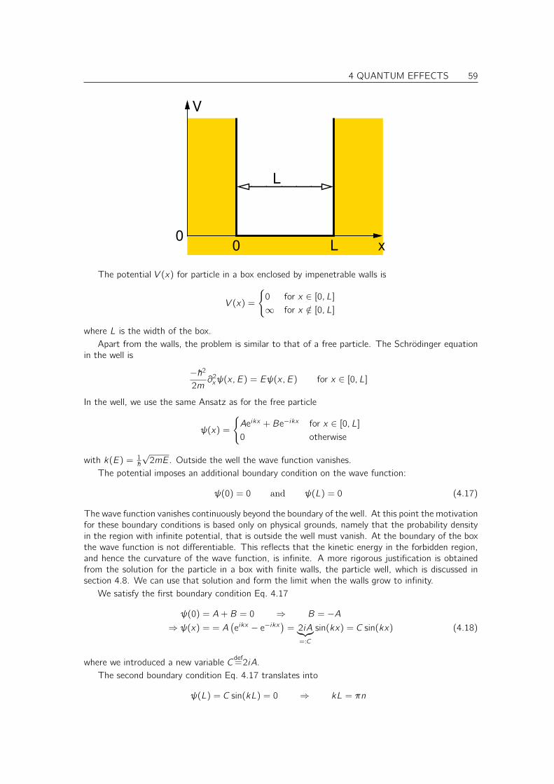
4 QUANTUM EFFECTS 59
L
L0
x
V
0
The potential V (x) for particle in a box enclosed by impenetrable walls is
V (x) =
0 for x ∈ [0, L]
∞ for x /∈ [0, L]
where L is the width of the box.Apart from the walls, the problem is similar to that of a free particle. The Schrödinger equation
in the well is
−~2
2m∂2xψ(x, E) = Eψ(x, E) for x ∈ [0, L]
In the well, we use the same Ansatz as for the free particle
ψ(x) =
Aeikx + Be−ikx for x ∈ [0, L]
0 otherwise
with k(E) = 1~√
2mE. Outside the well the wave function vanishes.The potential imposes an additional boundary condition on the wave function:
ψ(0) = 0 and ψ(L) = 0 (4.17)
The wave function vanishes continuously beyond the boundary of the well. At this point the motivationfor these boundary conditions is based only on physical grounds, namely that the probability densityin the region with infinite potential, that is outside the well must vanish. At the boundary of the boxthe wave function is not differentiable. This reflects that the kinetic energy in the forbidden region,and hence the curvature of the wave function, is infinite. A more rigorous justification is obtainedfrom the solution for the particle in a box with finite walls, the particle well, which is discussed insection 4.8. We can use that solution and form the limit when the walls grow to infinity.
We satisfy the first boundary condition Eq. 4.17
ψ(0) = A+ B = 0 ⇒ B = −A⇒ ψ(x) = = A
(eikx − e−ikx
)= 2iA︸︷︷︸
=:C
sin(kx) = C sin(kx) (4.18)
where we introduced a new variable Cdef=2iA.
The second boundary condition Eq. 4.17 translates into
ψ(L) = C sin(kL) = 0 ⇒ kL = πn

60 4 QUANTUM EFFECTS
where n is an arbitrary integer.10
Thus the wave vector can assume one of the discrete values kn, where
kn =π
Ln (4.19)
The dispersion relation E = (~k)2/2m provides the corresponding energy eigenvalues.
En =(~kn)2
2m
Eq. 4.19=
( ~2π2
2mL2
)n2 (4.20)
where n is an integer11. Thus, in a box, only discrete wave vectors and eigenvalues are permitted.They are quantized.
0
5
10
15
20
25
0 0.2 0.4 0.6 0.8 1
Fig. 4.4: The lowest five wave func-tions of the particle in the box. Thevertical axis is the energy in units of~2π2/(2mL2). The energy value hasbeen taken as the zero axis for the cor-responding wave function. The latter isgiven in arbitrary units. Note that thelowest state is not at energy zero, whichis a consequence of the zero point vi-bration or Heisenberg’s uncertainty re-lation. Note that the wave functionscan be classified according to their be-havior under mirror operation about thecenter of the box: Some are symmetricand some are antisymmetric. This is aconsequence of the mirror symmetry ofthe potential. Note that the number ofnodes (the zeros) increases with energy.Also this is a general feature of Problemswith a local potential.
Finally we need to normalize the wave function, which determines C.
∫ ∞−∞
dx ψ∗(x)ψ(x) = 1
10The zeros of the sinus function lie at multiples of π.11integer number=ganze Zahl

4 QUANTUM EFFECTS 61
2E
1E
3E
k
E
zero−point energy
trivial solution ϕ=0
Fig. 4.5: The energy levels for a particle in a box are obtained from the dispersion relation E(k) ofa free particle by selecting equi-distant values kn = π
L n for the k-points. The spacing of the k-pointschanges inversely with the size of the box. The number of nodes increase with energy. Note thatthe wave function for k = 0 does not exist, because it is identical to zero. Every wave function isa standing wave composed of two plane waves with positive and negative k . They are shown in theinsets.
which implies
1 =
∫ ∞−∞
dx ψ∗(x)ψ(x)Eq. 4.18
=
∫ L
0
dx C∗C sin2(knx)
= C∗C
∫ L
0
dx
(1
2−
1
2cos(2knx)
)= C∗C
L
2
⇒ |C| =
√2
L
We may use C as real number.Thus we obtain the wave functions and their energies as
ψn(x) =
√2
Lsin(knx) with kn
Eq. 4.19=
π
Ln
EnEq. 4.20
=~2π2
2mL2n2
We make some interesting observations:
• The lowest energy is not zero! Since the particle in the box has only kinetic energy, this impliesthat the particle can not be at rest.12 This effect, which is a general feature of bound systems,is called the zero-point motion and the corresponding energy is called zero-point energy.
We observe here an effect of Heisenberg’s uncertainty principle, which says that the positionand the momentum of a particle cannot be determined simultaneously with absolute certainty.
12Note that we use here the language from classical mechanics for a quantum particle.

62 4 QUANTUM EFFECTS
If the particle were at rest, its momentum would be zero and therefore certain. Consequently,the position should be completely unknown, which contradicts with the fact that the particle isconfined in a box. The smaller the box the larger is the zero point energy. We will later learnabout a more rigorous formulation of Heisenberg’s uncertainty principle.
Loosely termed, Heisenberg’s uncertainty principle says that one cannot form a localized wavepacket with a single plane wave. Very localized wave packets require large sets of plane wavesand therefore have wide distribution of momenta. The average momentum, on the other handis still a single quantity. In a language of particles, the uncertainty principle is most puzzling.However, in a wave description it is almost a triviality.
In a classical description an electron would fall right in the nucleus, since as accelerated chargedparticles it emits electromagnetic waves, and therefore looses energy. The zero point energyprevents this process.
• The allowed energies are quantized, that is they are discrete. This implies that we cannotadd energy to the system or remove energy from the system in arbitrary amounts. The energyspacing is inversely proportional with the mass of the particle. Hence, for a very heavy particleit would not be observable and the behavior would appear classical.
A word of caution is required here. The quantization only concerns stationary states. It ispossible to prepare a state with arbitrary energies. This state however is not a stationary state,but a superposition of stationary states, which has a probability distribution that changes withtime.
• The number of nodes in the wave function increases with the energy. This is a general propertyof second order differential equations in one dimension having a local potential. This statementis a consequence of the nodal-line theorem or Knotensatz by Richard Courant[21].(see alsoAppendix F on p. 271)
4.5.1 Time-dependent solutions for the particle in the box
Note that the solutions for the stationary Schrödinger equation, provide us with the energy levels,but not with the dynamics of a general wave function. A general wave function has the form
ψ(x, t) =
∞∑n=1
φn(x)e−i~ εntan
where the coefficients an are determined by the initial conditions of the problem.Let us consider several situations:
• If only one eigenstate contributes, so that
ψ(x, t) = φn(x)e−i~ εnt
we observe that the probability density
P (x, t) = ψ∗n(x, t)ψn(x, t) = φ∗n(x)φn(x)
does not change with time. Note that this is also true for excited states. This is the reasonthat one calls these solutions stationary. The wave function itself, however, oscillates. Thehigher the energy the faster the oscillation.
• Consider now the superposition of the first and the second eigenstate
ψ(x, t) = φ1(x)e−i~ ε1ta1 + φ2(x)e−
i~ ε2ta2

4 QUANTUM EFFECTS 63
The probability density is no more constant in time
P (x, t) = ψ∗(x, t)ψ(x, t) =(φ∗1(x)ψ1(x)a∗1a1 + φ∗2(x)ψ2(x)a∗2a2
)+2Re
(φ∗1(x)φ2(x)a∗1a2 e−
i~ (ε1−ε2t
)
Fig. 4.6: Probability density P(x,t) for a superposition of ground and first excited state of the particlein the box as function of time. The time axis points from the front to the back.
The term that does not vary in time is mirror-symmetric, while the oscillating term is antisym-metric. This indicates that the particle oscillates back an forth with circular frequency given by~ω = ε2 − ε1. If the particle is charged, the particle acts like an antenna and it sends out elec-tromagnetic radiation, i.e. light. The circular frequency of the radiation is ω, which indicatesthat light is emitted only with certain spectral lines corresponding to the energy differencesif the discrete energy eigenlevels. Thus the system looses energy until it ends up in a pureeigenstate, which in this case is the ground state.13 This is a first indication that atoms andmolecules end up after a certain while in pure eigenstates of the Hamilton operator.
• How does the quantum mechanical result relate to the classical result? Let us create a wavepacket and follow its motion.
We start from the general Ansatz for the wave function as superposition of the solutions ofthe time-independent Schrödinger equation. The time dependence is included by attaching the
13This is not obtained from the Schrödinger equation in the present form, because the electromagnetic fields do notenter the Hamiltonian.

64 4 QUANTUM EFFECTS
phase e−iωnt = e−i~ εnt to each eigenstate φn(x).
ψ(x, t) =
∞∑n=1
√2
Lsin(knx)︸ ︷︷ ︸φn(x)
e−iω(kn)tan
=
∞∑n=1
√2
L
1
2i
(ei(knx−ω(kn)t) − e−i(knx+ω(kn)t)
)an
=
∞∑n=1
ei(knx−ω(kn)t) 1
i√
2Lan︸ ︷︷ ︸
ψ1(x,t)
−∞∑n=1
e−i(knx+ω(kn)t) 1
i√
2Lan︸ ︷︷ ︸
ψ2(x,t)
The solution seems to consist of two wave packets, ψ1(x, t) and ψ2(x, t), running in oppositedirections. There is even more to it: we can show that each of the two solution actually isan array of partner solutions separated by a distance of 2L. These presence of those periodicimages is due to the equispaced discrete grid of wave vectors.
ψ1(x, t) =
∞∑n=1
ei(knx−
−2πn︷ ︸︸ ︷2knL−ω(kn)t) 1
i√
2Lan =
∞∑n=1
ei(kn(x−2L)−ω(kn)t) 1
i√
2Lan
= ψ1(x − 2L, t) (4.21)
In our problem, the periodic images are not real because at most one of them is located in thebox. The other partners are only mathematical artifacts. Nevertheless they allow us to imaginethe processes that occur.
The two solutions ψ1(x, t) and ψ2(x, t) are also related by a geometric transformation: theyare mirror images at the mirror plane at the right wall of the box, x = 0.
ψ2(x, t) =
∞∑n=1
e−i(knx+ω(kn)t) 1
i√
2Lan =
∞∑n=1
ei(kn(−x)−ω(kn)t) 1
i√
2Lan = ψ1(−x, t) (4.22)
Furthermore, there is a mirror plane at the right wall of the box, x = L.
ψ2(x − L)Eq. 4.22
= ψ1(−x + L)Eq. 4.21
= ψ1(−x − L)
We choose the initial conditions such that the solution ψ1(x, t) is a wavepacket somewhereinside the box and with a velocity vg. Our analysis tells us that this wave packet will move toone the walls, where it disappears “in the wall”. While this wave packet disappears, one of theperiodic images of ψ2(x, t) appears out “of the wall”. At the walls these two solutions exactlycancel consistent with the requirement that the wave function goes to zero at the boundariesof the box. The wave packet ψ2(x, t) moves to the opposite wall, where it disappears. At thesame time the next periodic image of ψ1(x, t) is ready to appear out of the wall. The result isthat the wave packet bounces back and forth exactly as a classical particle would do. As thewave packet moves back an forth, it delocalizes exactly as we described it for the free particle.
2L2L

4 QUANTUM EFFECTS 65
4.6 Potential step and splitting of wave packets
The potential step is the basic building block for a large class of problems that can be solved fairlyeasily. The potential step will also make us familiar with a new quantum effect, namely the splittingof wave packets.
Imagine an interface between a metal and a semiconductor. Electrons can propagate in the semi-conductor, if they have sufficient energy to enter the conduction band. Thus the electrons experiencea potential step. Metal-semiconductor interface are present at electric contacts to semiconductordevices, so-called Schottky contacts. They are the key element of Schottky-diodes used as rectifiers.
V∆
III
V
I
V
x
II
VI
The problem is defined as follows: Space is divided into two regions, region I for x < 0 and regionII for x > 0. In region I we have a constant potential VI and a solution ψI and in region II we have apotential VII and a solution ψII so that
V (x) = θ(−x)VI + θ(x)VII
ψ(x) = θ(−x)ψI(x) + θ(x)ψII(x)
where θ(x) is the Heaviside function or step function defined by
θ(x) =
0 for x < 012 for x = 0
1 for x > 0
.
4.6.1 Kinetic energy larger than the potential step
Let us first consider the case when the energy is sufficient to mount the step. A classical particle insuch a situation will always mount the step and proceed with a smaller velocity as some of its kineticenergy has been used up to mount the step. For a quantum particle everything is different.
For a given energy, the energy eigenstates are
ψI(x) = AeikIx + Be−ikIx
ψII(x) = CeikIIx +De−ikIIx (4.23)
with
~kI =√
2m(E − VI) and ~kII =√
2m(E − VII) (4.24)
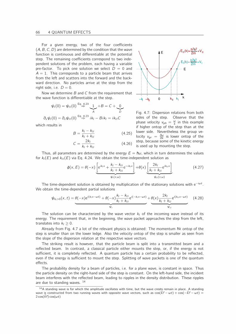
66 4 QUANTUM EFFECTS
kII II−k
2
2m+VIEI(k)=
h2k2
2mEII (k)= +VII
k0
E
E
−kI kI
h2k
Fig. 4.7: Dispersion relations from bothsides of the step. Observe that thephase velocity vph = ω
k in this exampleif higher ontop of the step than at thelower side. Nevertheless the group ve-locity vgr = ∂ω
∂k is lower ontop of thestep, because some of the kinetic energyis used up by mounting the step.
For a given energy, two of the four coefficients(A,B, C,D) are determined by the condition that the wavefunction is continuous and differentiable at the potentialstep. The remaining coefficients correspond to two inde-pendent solutions of the problem, each having a variablepre-factor. To pick one solution we select D = 0 andA = 1. This corresponds to a particle beam that arrivesfrom the left and scatters into the forward and the back-ward direction. No particles arrive at the step from theright side, i.e. D = 0.
Now we determine B and C from the requirement thatthe wave function is differentiable at the step.
ψI(0) = ψII(0)Eq. 4.23⇒ 1︸︷︷︸
A
+B = C + 0︸︷︷︸D
∂xψI(0) = ∂xψII(0)Eq. 4.23⇒ ikI − BikI = ikIIC
which results in
B =kI − kIIkI + kII
(4.25)
C =2kI
kI + kII(4.26)
Thus, all parameters are determined by the energy E = ~ω, which in turn determines the valuesfor kI(E) and kII(E) via Eq. 4.24. We obtain the time-independent solution as
φ(x, E) = θ(−x)
[eikIx +
kI − kIIkI + kII
e−ikIx]
︸ ︷︷ ︸ψI(x,ω)
+θ(x)
[2kI
kI + kIIeikIIx
]︸ ︷︷ ︸
ψII(x,ω)
(4.27)
The time-dependent solution is obtained by multiplication of the stationary solutions with e−iωt .We obtain the time-dependent partial solutions
ψkI>0(x, t) = θ(−x)ei(kIx−ωt) + θ(−x)kI − kIIkI + kII
ei(−kIx−ωt)︸ ︷︷ ︸ΨI
+ θ(x)2kI
kI + kIIei(kIIx−ωt)︸ ︷︷ ︸
ΨII
(4.28)
The solution can be characterized by the wave vector kI of the incoming wave instead of itsenergy. The requirement that, in the beginning, the wave packet approaches the step from the left,translates into kI ≥ 0.
Already from Fig. 4.7 a lot of the relevant physics is obtained: The momentum ~k ontop of thestep is smaller than on the lower ledge. Also the velocity ontop of the step is smaller as seen fromthe slope of the dispersion relation at the respective wave vectors.
The striking result is however, that the particle beam is split into a transmitted beam and areflected beam. In contrast, a classical particle either mounts the step, or, if the energy is notsufficient, it is completely reflected. A quantum particle has a certain probability to be reflected,even if the energy is sufficient to mount the step. Splitting of wave packets is one of the quantumeffects.
The probability density for a beam of particles, i.e. for a plane wave, is constant in space. Thusthe particle density on the right-hand side of the step is constant. On the left-hand side, the incidentbeam interferes with the reflected beam, leading to ripples in the density distribution. These ripplesare due to standing waves. 14
14A standing wave is for which the amplitude oscillates with time, but the wave crests remain in place. A standingwave is constructed from two running waves with opposite wave vectors, such as cos(~k~r − ωt) + cos(−~k~r − ωt) =2 cos(~k~r) cos(ωt)

4 QUANTUM EFFECTS 67
The situation described here is rather similar to the refraction of light at the surface of an opticallydenser medium. Partial reflection and partial transmission at an interface is a well known observation.However some properties differ: For a particle with a mass, the momentum ~k is smaller ontop ofthe barrier than on the lower ledge. For light entering a denser medium the wave vector grows larger.As a result the angle of refraction is smaller than the incident angle for light, while for particles it islarger than the incident angle.
4.6.2 Construct the other partial solution using symmetry transformations
A second-order differential equation in one dimension has always two linear independent solutions.In order to obtain the general solution, we need to construct one other independent solution of theproblem.
The second partial solution can be obtained using symmetry arguments from the one just derivedand presented in Eq. 4.28. Using symmetry arguments to construct solutions is an extremely powerfultechnique that allows one to save a lot of computations. This is why I describe this example in somedetail:
II II II II I
The second partial solution shall describe a wave packet, which approaches the step from the right(higher) side and which hops down the step. We construct this solution by two successive transfor-mations of the problem.
1. First we apply a mirror operation at the step. The Schrödinger equation remains independentexcept for the potential. The new potential V ′(x) = V (−x) describes a step with the upperside on the left. The partial solution given in Eq. 4.28 is transformed by interchanging x by−x , i.e. x ′ = −x , so that ψ′(x, t) = ψ(−x, t).
ψ′(x ′, t) = ψkI>0(x, t)
⇒ ψ′(x, t) = ψkI>0(−x, t)
⇒ ψ′(x, t)Eq. 4.28
= θ(x)ei(−kIx−ωt) + θ(x)kI − kIIkI + kII
ei(+kIx−ωt)︸ ︷︷ ︸Ψ′II
+ θ(−x)2kI
kI + kIIei(−kIIx−ωt)︸ ︷︷ ︸
Ψ′I
We have defined Ψ′I = ΨII(−x, t) so that it describes the transformed solution on the left sideof the step and Ψ′II = ΨI(−x, t) described the transformed solution on the right of the step.
The solution obtained after this operation describes a particle approaching the step from theright-hand side, which is partially reflected and which partially hops up the step.
2. In a second operation, we restore the original potential: We interchange VI and VII , so thatthe elevated part of the step is again on the right hand side. We need to control that thederivation of Eq. 4.28 does not make use that VII > VI . The second transformation transformsV ′′I = V ′II = VII and V ′′II = V ′I = VI . This implies replacing kI and kII , i.e. k ′′II = kI and k ′′I = kII .In this way, we obtain our final result for the second partial solution.
ψ′′(x, t) = θ(x)ei(−kIIx−ωt) − θ(x)kI − kIIkI + kII
ei(+kIIx−ωt)︸ ︷︷ ︸Ψ′′II
+ θ(−x)2kII
kI + kIIei(−kIx−ωt)︸ ︷︷ ︸
Ψ′′I
(4.29)

68 4 QUANTUM EFFECTS
In summary, the second solution ψ′′(x, t) given in Eq. 4.29 is obtained from the first partialsolution in Eq. 4.28 by the transformation
x ′ = −x and k ′II = kI and k ′I = kII .
This solution ψ′′ describes a beam of particles approaching from the right, that is partially reflectedand partially transmitted down the potential step. Surprisingly, we observe that the particle arepartially reflected even at a downhill step.
Scattering of wave packets
In order to explore the physical content of these solutions, let us consider the scattering of a wavepacket. We may choose one that approaches the step from the left side with coefficients a(k).
ψ1(x, t) = χ(x, t)ei(kIx−ω(kI)t) =
∫dk
2πa(k)ei(kx−ω(k)t) (4.30)
ψ1(x, t) describes the initial wave packet before it arrives at the potential step.If the wave packet is localized initially in region I, it can be expressed entirely by partial solutions
given in Eq. 4.28. The wave packet can then be expressed by three wave packets, which we denoteas Ψ1,Ψ2 and Ψ3. The first one is, per construction, our initial wave packet Eq. 4.30.
ψ(x, t)Eq. 4.28
=
∫dkI2π
a(kI)[θ(−x)ei(kIx−ωt) + θ(−x)B(kI)ei(−kIx−ωt) + θ(x)C(kI)ei(kIIx−ωt)
]= θ(−x)
∫dkI2π
a(kI)ei(kIx−ωt)︸ ︷︷ ︸ψ1
+θ(−x)
∫dkI2π
a(kI)B(kI)ei(−kIx−ωt)︸ ︷︷ ︸ψ2
+ θ(x)
∫dkI2π
a(kI)C(kI)ei(kIIx−ωt)︸ ︷︷ ︸ψ3
= θ(−x)ψ1(x, t) + θ(−x)ψ2(x, t) + θ(x)ψ3(x, t) (4.31)
The coefficients B(kI) and C(kI) are those of Eq. 4.25 and Eq. 4.26. The wave packet ψ1(x, t)describes the incoming particles. The wave packed ψ2(x, t) describes the reflected wave particlesand the wave packet ψ3(x, t) describes the particles transmitted through the barrier.
In order to simplify the discussion, let us choose a very smooth envelope function for the wavepacket so that the wave function coefficients a(k) are localized near a given wave vector k . Then Ican approximate B(k) and C(k) by the value at k .
ψ2(x, t)Eq. 4.31
=
∫dkI2π
a(kI)B(kI)ei(−kIx−ωt)
≈ B(kI)
∫dkI2π
a(kI)ei(−kIx−ωt)
= B(kI)ψ1(−x, t) Eq. 4.25=
kI − kIIkI + kII
ψ1(−x, t) (4.32)
Thus, the reflected wave packet is identical to the incoming wave packet, but mirrored at the stepand reduced in size by the prefactor B(kI). While the incoming wave disappears at the step due tothe step function, the reflected wave appears “from under its own step function”.
Let us now consider the third wave packet ψ3(x, t): Here the wave vector kII occurs in the planewave. Since both, kI and kII , are linked to the energy, one can also express kII as function of kI . Weuse Eq. 4.24
~2k2II = 2m(E − VII) ∧ ~2k2
I = 2m(E − VI)⇒ ~2k2
II − ~2k2I = −2m(VII − VI) = −2m∆V
⇒ kII(kI) =√k2I − 2m∆V/~2 (4.33)

4 QUANTUM EFFECTS 69
Because only values of kI close to kI contribute appreciably to the integral, we replace this functionby its Taylor expansion about kI :
kII(kI) = kII(kI)︸ ︷︷ ︸kII
+∂kII∂kI
∣∣∣∣kI︸ ︷︷ ︸
=kI/kII
(kI − kI) +O(kI − kI)2
Eq. 4.35= kII +
kI
kII(kI − kI) +O(kI − kI)2 (4.34)
We inserted here the derivative
∂kII∂kI
∣∣∣∣kI
Eq. 4.33=
1
2
2kI√k2I − 2m∆V/~2
Eq. 4.33=
kI
kII(kI)
kIIdef=kII(kI=
kI
kII(4.35)
We use this expression in the following when we determine the relation between ψ3 and ψ1.
ψ3(x, t)Eq. 4.31
=
∫dkI2π
a(kI)C(kI)ei(kII(kI)x−ωt)
≈ C(kI)
∫dkI2π
a(kI)ei(
≈kII (kI )︷ ︸︸ ︷[kII +
kI
kII(kI − kI)
]x−ωt)
= C(kI)ei(kII−
kIkIIkI)x∫dkI2π
a(kI)ei(
kIkIIkIx−ωt)︸ ︷︷ ︸
=ψ1(∂kII∂kI
x,t)
(4.36)
Now we represent the incoming wave packet by a plane wave part and an envelope function
ψ1(x, t)Eq. 4.30
= χ(x, t)ei(kIx−ωt) (4.37)
ψ3(x, t)Eq. 4.36
= C(kI)ei(kII−
kIkIIkI)xψ1(
kI
kIIx, t)
Eq. 4.37= C(kI)e
i(kII−kIkIIkI)xχ(
kI
kIIx, t)e
i(kIkIkIIx−ωt)
= C(kI)χ(kI
kIIx, t)ei(kIIx−ωt)
Eq. 4.26=
2kI
kI + kIIχ(kI
kIIx, t)ei kIIx−ωt (4.38)
Thus the transmitted wave packet ψ3 can again be related to the incoming wave packet ψ1 by a fewtransformations:
• The leading wave kI vector is replaced by a smaller one, namely kII .
• The envelope function χ(x, t) is compressed by the factor kII/kI
• The velocity of the wave packet is reduced by the same factor kII/kI .
• The amplitude is reduced by the factor CEq. 4.26
= 2kIkI+kII
Thus we can obtain the wave packets Ψ2 and Ψ3 from Ψ1 by simple geometric operations and arescaling of the amplitude and main wave vector. Ψ2 is a simple mirror image of Ψ1 and approachesthe step from the right side. Ψ3 is located on the same side as Ψ1 but it is stretched. While Ψ3 hasabout the same envelope function as Ψ1, the envelope function modulates a different plane wave.

70 4 QUANTUM EFFECTS
Fig. 4.8: schematic representation of a 2-dimensional wave packet scattering at a potential step.The lines represent the wave crests. The white areas represent the shape of the wave packet. Thearrows indicate the velocity, respectively the wave vector.
Initially the wave function Ψ is equal to Ψ1 and it is localized in the left half plane. Ψ2 and Ψ3 donot appear yet because they are localized in that half plane, where the corresponding step functionvanishes. The wave packet approaches the step from the left-hand side. When it hits the step, Ψ1
starts to disappear under its step function. At the same time the wave packets Ψ2 and Ψ3 appearfrom under their step functions, so that Ψ1 is gradually replaced by Ψ2 and Ψ3. The wave packetΨ2 describes the particles reflected to the left, while Ψ3 describes the particles transmitted to theright.
Reflection and transmission coefficient
The weight of the reflected wave packet is called the reflection coefficient
Rdef=
∫dx ψ∗2(x)ψ2(x)
Eq. 4.32=
|kI − kII |2
|kI + kII |2
It is the probability that a particle is reflected at the potential step.The probability that the wave packet transmitted is called transmission coefficient.
Tdef=
∫dx ψ∗3(x)ψ3(x) = |C(kI)|2
∫dx ψ∗1(
kI
kIIx)ψ1(
kI
kIIx) = |C(kI)|2
kII
kI
∫dx ψ∗1(x)ψ1(x)
=|kII ||kI |
|2kI |2
|kI + kII |2︸ ︷︷ ︸|C(kI)|2
=4|kI ||kII ||kI + kII |2
It is easily seen that R + T = 1, that is the particle is either transmitted or reflected. R/T issmall when the kinetic energy of the incoming wave packet is much larger than the size of the step.Thus we recover the classical result in this limit. When the energy is barely sufficient to mount thestep, that is when kII approaches zero, the reflection coefficient becomes unity.
Thus the wave packet splits at the step in two pieces. Such a behavior is impossible for a classicalparticle, which always maintains its integrity. If its energy is sufficient it will always climb up thestep, and does not reflect. For a wave it is not surprising it can be split. A beam of light, that iselectromagnetic waves, can be partially reflected and partially transmitted through a window of glass.

4 QUANTUM EFFECTS 71
The reflection and transmission coefficients as function of the energy is shown in Fig. 4.9.
TR
V E
1
0
Fig. 4.9: Transmission (green) and reflection coefficient (golden) for a step of height V as functionof energy. The transmission coefficient vanishes when the energy is lower than the step height andit approaches unity for high energies.
What does it mean when the wave packet splits? The particle is not really divided into two distinctpieces. The wavefunction provides us only with the probability to find the particle somewhere in space.Hence a splitting wave packet tells us that the particle has a finite probability to pass on or to bereflected.
There is one open question: Why do we not observe this beam splitting for macroscopic particles?The answer lies in the abruptness of the potential step. A macroscopic potential step is not abrupt.If the wave packet is small compared to the region over which the potential changes from one valueto another, the transmission coefficient approaches one and the wave packet behaves like a classicalparticle. 15
Interestingly also a wave packet hopping down the step is reflected with finite probability.It is possible to evaluate the transmission and reflection coefficients without using wave packets.
What we need are the amplitudes and wave vectors of the transmitted and reflected waves, that isEqs. 4.24,4.25 and 4.26. We can evaluate the particle current as density times velocity, that is
j(x) = Ψ∗(x)Ψ(x)∂ω
∂k︸︷︷︸vg
= Ψ∗(x)Ψ(x)~km
Thus we can define the reflection coefficient as the ratio of reflected versus incoming current andthe transmission coefficient as the ratio of transmitted versus incoming current.
T =j3j1
=|C|2kIIkI
=4kIkII
(kI + kII)2
R =j2j1
= |B|2 =(kI − kII)2
(kI + kII)2
Note that both, kI and kII are functions of the energy, and therefore transmission and reflectioncoefficient are functions of the energy as well.
15This can be seen as follows: we divide the potential step into many smaller steps, so that the total height ispreserved. Each plateau of the potential must be much larger than the size of the wave packet. The total transmissioncoefficient is then the product of the transmission coefficients of the smaller steps. If the step is divided into manysmall steps, the total transmission coefficient tends to one. (Hint: Use steps ki = kIe
αi/n with eα = kII/ki )
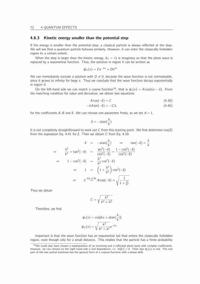
72 4 QUANTUM EFFECTS
4.6.3 Kinetic energy smaller than the potential step
If the energy is smaller than the potential step, a classical particle is always reflected at the step.We will see that a quantum particle behaves similarly. However, it can enter the classically forbiddenregion to a certain extent.
When the step is larger than the kinetic energy, kII = iλ is imaginary so that the plane wave isreplaced by a exponential function. Thus, the solution in region II can be written as
ψII(x) = Ce−λx +Deλx
We can immediately exclude a solution with D 6= 0, because the wave function is not normalizable,since it grows to infinity for large x . Thus we conclude that the wave function decays exponentiallyin region II.
On the left-hand side we can match a cosine function16, that is ψI(x) = A cos(kx − δ). Fromthe matching condition for value and derivative, we obtain two equations
A cos(−δ) = C (4.39)
−kA sin(−δ) = −Cλ (4.40)
for the coefficients A,B and δ. We can choose one parameter freely, so we set A = 1.
δ = −atan(λ
k)
It is not completely straightforward to work out C from this starting point. We first determine cos(δ)from the expression Eq. 4.41 for δ. Then we obtain C from Eq. 4.39.
δ = −atan(λ
k) ⇒ tan(−δ) =
λ
k
⇒λ2
k2= tan2(−δ) =
sin2(−δ)
cos2(−δ)=
1− cos2(−δ)
cos2(−δ)
⇒ 1− cos2(−δ) =λ2
k2cos2(−δ)
⇒ 1 =
(1 +
λ2
k2
)cos2(−δ)
⇒ CEq. 4.39
= A cos(−δ) =
√1
1 + λ2
k2
Thus we obtain
C =
√k2
k2 + λ2
Therefore, we find
ψI(x) = cos[kx + atan(λ
k)]
ψII(x) =
√k2
k2 + λ2e−λx
Important is that the wave function has an exponential tail that enters the classically forbiddenregion, even though only for a small distance. This implies that the particle has a finite probability
16We could also have chosen a superposition of an incoming and a reflected plane wave with complex coefficients.However, we can choose on the right hand side a real dependence, i.e. Im[C] = 0. Then also ψI(x) is real. The realpart of the two partial solutions has the general form of a cosinus function with a phase shift.

4 QUANTUM EFFECTS 73
to enter the classically forbidden region. For a classical particle this is impossible. The same effectwill lead us later to the effect of tunneling: A quantum particle can even penetrate a hard wall if itis sufficiently thin.
The exponential damping of the wave function in region II corresponds to total reflection of light.If we try to look through the water surface into the pond, there is a viewing certain angle wherethe water surface reflects completely and all that is underneath the surface is hidden from us. If westand up and peek into the water at a steeper angle, we suddenly observe that the water becomesmore transparent.
4.6.4 Logarithmic derivative
Before we continue, we will learn a useful way to solve matching problems. The general problem isone of two regions in a one-dimensional space. We assume that we have only one solution ψ3 inregion II, and the superposition of two solutions ψ1 and ψ2 in region I. Without limitation of generalitywe choose region I to be the region left of x = 0 and region II to be the region right of x = 0.
In the case of the potential step we have selected one outgoing wave ψ3 = eikx in region II, butno incoming wave. In region I we have a superposition of ψ1 and ψ2. The Ansatz for the wavefunction is
Ψ(x) = θ(−x)[AΨ1(x) + BΨ2(x)
]+ θ(x)Ψ3(x) (4.41)
Without loss of generality, I have chosen x = 0 as the boundary between the regions I (x < 0) and II(x > 0). θ(x) is the Heaviside function with θ(x < 0) = 0 and θ(x > 0) = 1. Thus θ(x) equals onefor region II and vanishes in region I, while θ(−x) equals one for region I and vanishes for region II.
The matching problem has the following form, where we abbreviate ψidef=ψi(0) and ∂xψi
def=∂x |0ψi .(
ψ1 ψ2
∂xψ1 ∂xψ2
)(A
B
)=
(ψ3
∂xψ3
)where values and derivatives are taken at the boundary x = 0 between the two regions I and II. Aftermultiplication with the inverse of the matrix on the left hand side, we obtain the coefficients A andB (
A
B
)=
1
ψ1∂xψ2 − ψ2∂xψ1
(∂xψ2 −ψ2
−∂xψ1 ψ1
)(ψ3
∂xψ3
)
=1
ψ1ψ2(D2 −D1)
(ψ2ψ3(D2 −D3)
ψ1ψ3(D3 −D1)
)(4.42)
where we used the shorthand notation Di = Dψi (0) for the logarithmic derivative defined below.
Definition 4.1 LOGARITHMIC DERIVATIVE
Dψ(x0) =∂x |x0
ψ(x)
ψ(x0)= ∂x |x0
ln[ψ(x)] (4.43)
The logarithmic derivative is independent of a scale factor, that is of the normalization.
Thus we find the solution17 for the solution that is valid across the boundary.
ψEqs. 4.41,4.42
= ψ3(0)θ(−x)[ψ1(x)
ψ1(0)
D2 −D3
D2 −D1+ψ2(x)
ψ2(0)
D1 −D3
D1 −D2
]+ θ(x)ψ3(x) (4.44)
17It is not required to memorize this equation itself, but only its derivation.

74 4 QUANTUM EFFECTS
Using this formula we can easily do the matching for a system with many potential steps. Onesimply chooses one partial solution on one end of the steps, which plays the role of ψ3(x). Then onematches the solution of the next segment to ψ3(x). The new solution in this segment now plays therole of ψ3(x) to do the matching across the next boundary. In this ways one can proceed step bystep from one end to the other and thus obtains one partial solution for the entire problem.
4.7 Barrier and tunnel effect
Let us consider a particle that approaches a barrier of finite width. If a classical particle approachessuch a situation, it will overcome the barrier, if its kinetic energy is sufficiently large, and if its energyis lower than the barrier, it will be reflected. There is no grey zone. However, we have seen for thepotential step, that the particle can penetrate a little into the step, even if its energy is insufficientto mount the step. This implies that if the barrier is sufficiently thin, there is a certain probabilitythat the particle appears on the other side of the step, even if that is classically forbidden. This isthe essence of the tunnel effect, which we will investigate here in some detail.
A famous application of the tunnel effect is the scanningtunneling microscopy18 , which is one of the very few experi-mental techniques that can make individual atoms visible. In thescanning tunneling microscope a very fine needle is brought intocontact with a surface. If a voltage is applied between the needleand the surface a current can flow. The distance between thetip of the needle and the surface is of the order of a nanome-ter. Due to the gap between surface and tip electrons cannotflow classically. However they can tunnel from surface to thetip. The resulting current is extremely sensitive to the distance,which is exploited to measure the topography of the surface andto control the motion of the tip.
I
x
V
I II III
0
L
V
In the following, we will determine the quantum mechanical behavior of particles impinging on abarrier. The potential has the following form
V (x) =
V0
0
for
0 < x < L
x < 0; x > L
We call the region to the left of the barrier region I, the barrier itself region II and what is to theright of the barrier is region III.
18Heinrich Rohrer and Gerd Binnig received, together with Ernst Ruska, the Nobel prize in Physics 1986 for theinvention of the Scanning tunneling microscope.

4 QUANTUM EFFECTS 75
The wave number of the particle in region I and III is kIVI=0= 1
~√
2mE. Two different cases needto be distinguished in the middle region II:
• Passing the barrier is classically allowed. That is the case of the kinetic energy in region I islarger than the barrier V0. The wave function is oscillatory in the barrier region with a wavevector kII = 1
~√
2m(E − VII) = 1~√
2m(E − V0)
• Passing the barrier is classically forbidden. In this case, the energy is below VII and the ki-netic energy in the barrier region is negative! A classical particle would be reflected by thebarrier. Instead of an oscillating solution we obtain a wave function that decays (or increases)exponentially with a decay constant λ = 1
~√
2m(V0 − E).
We begin with the case where the kinetic energy of the particle is sufficient to mount the barrier.We only sketch the outline of the derivation and leave the detailed derivation to appendix D.1 onp. 263. We form an Ansatz of the wave function
ψ(x) = θ(−x)ψI(x) + θ(x)θ(L− x)ψII(x) + θ(x − L)ψIII(x)
with the partial solutions for the three regions:
ψI(x) = AIeikIx + BIe
−ikIx
ψII(x) = AIIeikIIx + BIIe
−ikIIx
ψIII(x) = AIIIeikIx + BIIIe
−ikIx
The Ansatz has six unknowns.
• Four of the six unknowns are determined by the conditions that the wave function must be, ateach boundary, continuous with value and derivative. We call a wave function that is continuouswith value and derivative, differentiable.
• The remaining two variables can be determined by fixing the initial condition of a physicalproblem: If we are interested in a particle beam impinging from the left onto the barrier, wewould fix AI = 1 and BIII = 0. It is sufficient to determine two independent sets of initialconditions. Every other solution can be formed by superposition of these two partial solutions.
Of interest is how many of the impinging electrons are transmitted. Thus we evaluate thetransmission coefficient
T (E)def=
∣∣∣∣AIIIAI∣∣∣∣2
which we evaluated in the appendix in Eq. C.19 on p. 260. as
T (E)E>V=
1 +V 2
0
4E(E − V0)sin2(
L
~√
2m(E − V0)︸ ︷︷ ︸kIIL
)
−1
(4.45)
The result is shown in Fig. 4.11.The transmission coefficient has certain values where it becomes equal unity. Those states,
respectively their energies, are called resonances. The resonance can be understood as follows: Thewave packet on top of the barrier is partially reflected at the border of the barrier. If it is reflectedtwice it can positively interfere with itself. The interpretation would be that the particle is caughtinto a state with finite lifetime, where it remains for a while before it is transmitted again. Because itpauses on top of the barrier the probability density there is enhanced. In the resonance the particlesare not reflected at all by the barrier, but every particle is transmitted.
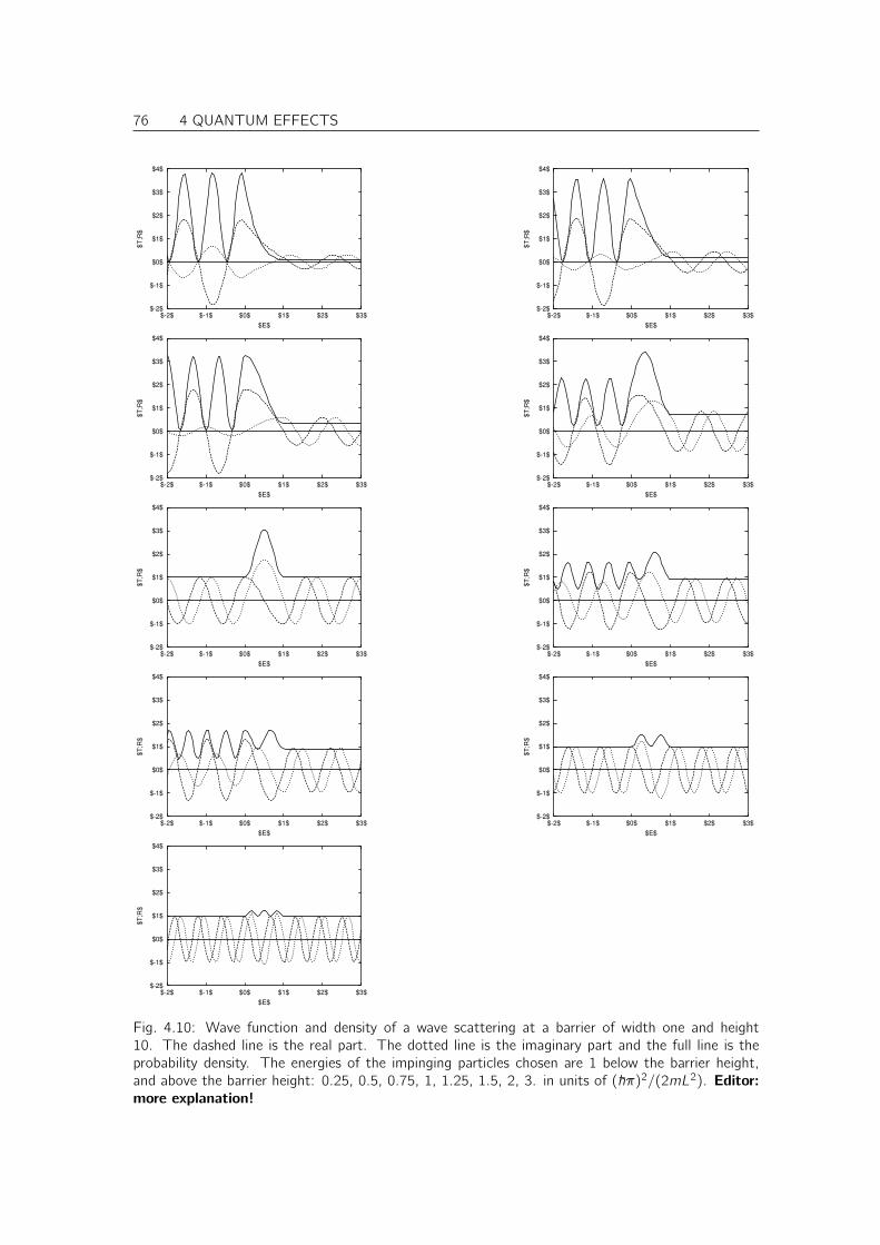
76 4 QUANTUM EFFECTS
$-2$
$-1$
$0$
$1$
$2$
$3$
$4$
$-2$ $-1$ $0$ $1$ $2$ $3$
$T
;R$
$E$
$-2$
$-1$
$0$
$1$
$2$
$3$
$4$
$-2$ $-1$ $0$ $1$ $2$ $3$
$T
;R$
$E$
$-2$
$-1$
$0$
$1$
$2$
$3$
$4$
$-2$ $-1$ $0$ $1$ $2$ $3$
$T
;R$
$E$
$-2$
$-1$
$0$
$1$
$2$
$3$
$4$
$-2$ $-1$ $0$ $1$ $2$ $3$
$T
;R$
$E$
$-2$
$-1$
$0$
$1$
$2$
$3$
$4$
$-2$ $-1$ $0$ $1$ $2$ $3$
$T
;R$
$E$
$-2$
$-1$
$0$
$1$
$2$
$3$
$4$
$-2$ $-1$ $0$ $1$ $2$ $3$
$T
;R$
$E$
$-2$
$-1$
$0$
$1$
$2$
$3$
$4$
$-2$ $-1$ $0$ $1$ $2$ $3$
$T
;R$
$E$
$-2$
$-1$
$0$
$1$
$2$
$3$
$4$
$-2$ $-1$ $0$ $1$ $2$ $3$
$T
;R$
$E$
$-2$
$-1$
$0$
$1$
$2$
$3$
$4$
$-2$ $-1$ $0$ $1$ $2$ $3$
$T
;R$
$E$
Fig. 4.10: Wave function and density of a wave scattering at a barrier of width one and height10. The dashed line is the real part. The dotted line is the imaginary part and the full line is theprobability density. The energies of the impinging particles chosen are 1 below the barrier height,and above the barrier height: 0.25, 0.5, 0.75, 1, 1.25, 1.5, 2, 3. in units of (~π)2/(2mL2). Editor:more explanation!

4 QUANTUM EFFECTS 77
5 6 9 140
1
0
E
R(E)
T(E)
Fig. 4.11: Transmission coefficient of a barrier of height 5 and width π/√
2. The transmissioncoefficient becomes nonzero, even if the energy is not sufficient to surmount the barrier classically.If the kinetic energy is larger than the barrier height, the transmission coefficient shows resonancesat those energies above the barrier, where the infinite well has its eigenvalues, i.e. E = V + (~π)2
2mL2 n2.
The origin for these resonances lies in the fact that the particle is reflected partly even if it jumpsdown a potential step.
In between the resonance energies the transmission coefficient is strongly suppressed, indicatingthat a large fraction of the particle beam is reflected.
Let us now consider the second case, where the kinetic energy of the incoming particle is smallerthan the barrier height. We can obtain the result for the transmission coefficient, by extending itinto the complex plane.
In this case, we have to express
sin(ix) =ei(ix) − e−i(ix)
2i=
e−x − ex
2i= i
ex − e−x
2= i sinh(x)
so that out of Eq. 4.45 we obtain the result for E < V
T (E) =
[1 +
V 20
4E(V0 − E)sinh2(
1
~√
2m(V0 − E)L)
]−1
(4.46)
which is identical to Eq. C.20 on p. 260.In that case, we see that the transmission coefficient Fig. 4.11 does not immediately drop to
zero. Even though a classical particle with that energy would be reflected a wave packet is partlytransmitted. This is the tunnel effect.
The tunnel effect is analogous to the observation that we can shine light through a very thinmetal foil. Even though the metal should reflect light completely, some of it can pass through, if thefoil is sufficiently thin.
4.8 Particle in a well and resonances
Let us consider a particle in a box with walls that allow it in principle to escape. This is a simplemodel for an electron bound by a nucleus. Given sufficient energy the electron may escape from thenucleus. This is the case we are considering here.
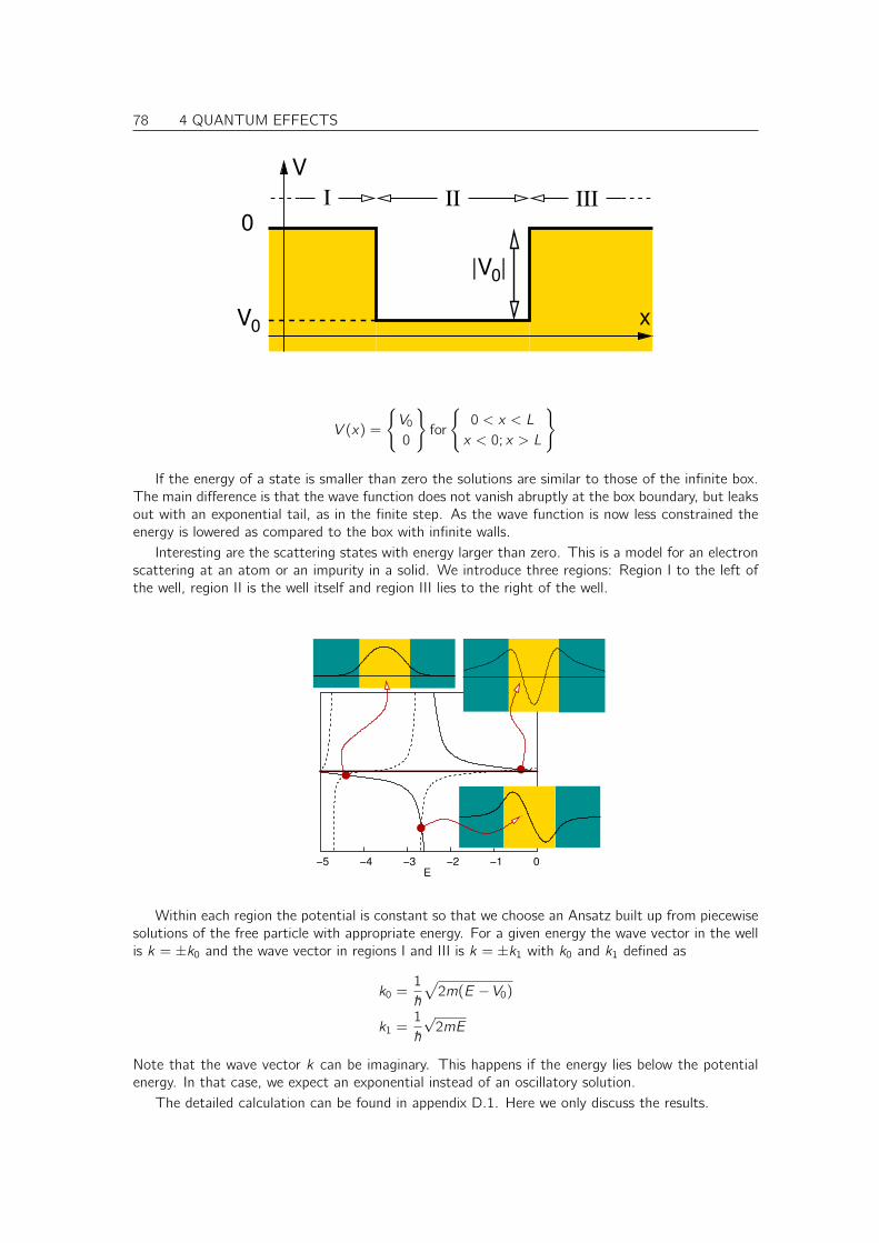
78 4 QUANTUM EFFECTS
0|
I
II
V
I III
xV
0
0
|V
V (x) =
V0
0
for
0 < x < L
x < 0; x > L
If the energy of a state is smaller than zero the solutions are similar to those of the infinite box.The main difference is that the wave function does not vanish abruptly at the box boundary, but leaksout with an exponential tail, as in the finite step. As the wave function is now less constrained theenergy is lowered as compared to the box with infinite walls.
Interesting are the scattering states with energy larger than zero. This is a model for an electronscattering at an atom or an impurity in a solid. We introduce three regions: Region I to the left ofthe well, region II is the well itself and region III lies to the right of the well.
E
−4 −2 0−3 −1−5
Within each region the potential is constant so that we choose an Ansatz built up from piecewisesolutions of the free particle with appropriate energy. For a given energy the wave vector in the wellis k = ±k0 and the wave vector in regions I and III is k = ±k1 with k0 and k1 defined as
k0 =1
~√
2m(E − V0)
k1 =1
~√
2mE
Note that the wave vector k can be imaginary. This happens if the energy lies below the potentialenergy. In that case, we expect an exponential instead of an oscillatory solution.
The detailed calculation can be found in appendix D.1. Here we only discuss the results.

4 QUANTUM EFFECTS 79
1
R
T
Fig. 4.12: Transmission coefficient of a potential well with depth V0 = −5 and width π/√
2. Thetransmission coefficient becomes unity at the resonances. The resonances, indicated by the doublearrows, lie at the energies, where the box with infinite walls has its eigenvalues, i.e. Ei = n2 − 5. Ifthe kinetic energy of the particle is large compared to the well depth, the particle does not experiencethe well any longer and the transmission coefficient becomes unity.
We obtain the transmission coefficient T =∣∣∣AIIIAI ∣∣∣2 as
TEq. C.19
=[
1 +V 2
4E(E − V )sin2
(L~√
2m(E − V0))]−1
The transmission coefficient has maxima where k0L0 = nπ, n being an integer, where it is unity.This is where the infinite potential well of same width has its eigenvalues. In between it drops toa value T = 4E(E−V )
(V−2E)2 , which is zero if the kinetic energy E outside the well vanishes, and whichapproaches one, if the kinetic energy is much larger then the well potential.
The energies, for which the transmission coefficient has its maxima, are called resonances. Atthose energies the electron is not reflected at all. The energies of the resonances can be estimatedfrom those of the particle in a box. They are approximately at
E ≈ V0 +~2π2
2mL2n2
4.9 Summary
We have learned that wave packet of a free particle becomes broader with time. This is due to thefact that probability distribution for the momenta is broad. Heisenberg’s uncertainty relation indicatesthat the momentum distribution is broader if the position distribution is narrow. If the dispersionrelation E(p) is non-linear the broad momentum distribution results in a broad velocity distribution.This velocity distribution is responsible for the broadening.
An energy eigenstate for the free particle is a simple plane wave with wave vector k = 1~√
2mEkinwhere Ekin = E − V is the kinetic energy. The higher the momentum of a particle, the smaller is itswave length.
For negative kinetic energy we would obtain exponentially decaying and increasing functions aseigenfunctions. They do not lead to eigenstates, because they violate the boundary conditions.
From the particle in the box we have seen that eigenstates are discrete, i.e. quantized, when theparticle is enclosed in a finite region.
The lowest energy for the particle in the box is not zero, but is has a minimum energy, thezero-point energy. This observation can again be rationalized by Heisenberg’s uncertainty relation,saying that a particle enclosed into a small spatial region has a large momentum uncertainty. This

80 4 QUANTUM EFFECTS
implies that the momentum cannot be zero, which implies that it has a finite kinetic energy. Thiszero-point energy becomes smaller the larger the box is. For an infinite box, that is for a free particle,the zero-point energy vanishes.
The energy eigenvalues for the particle in a box can be estimated from the quantization conditionfor the momenta, i.e. knL = πn, and the dispersion relation E(p) with the de-Broglie relation p = ~k .
A wave packet arriving at a potential step with a kinetic energy, that is sufficient to classicallymount the step, is split into a reflected and a transmitted wave package. If the energy is smaller thanthe barrier, the probability density does not disappear abruptly at the step, but the wave functionexhibits an exponential tail that enters the classically forbidden region. Nevertheless, all particles arereflected. For light, the exponential tails in the classically forbidden region correspond to the so-calledevanescent waves. If the kinetic energy is very different from the potential step, either much loweror much higher, the particle behaves classically, that is either the reflected or the transmitted wavepacket vanishes.
The potential well exhibits quantized energy levels for negative energies and a continuum ofscattering states for positive energies. The bound states are closely related to the states of the hardbox. It differs by the fact that the wave function does not go to zero abruptly at the boundaries ofthe box, but that it has exponential tails reaching out into the classical forbidden region. The energylevels are slightly below those of the hard box, because they have a little more room, because theycan leak out of the box a little.
For positive energies, the wave functions of the particle well are plane waves, that are modulatedin the well: The wave length is shorter, due to the larger kinetic energy and the probability densitymay be larger. The particle is partly reflected at each boundary of the well. Hence it can, after beingreflected twice, interfere constructively or destructively with the original wave. For constructiveinterference the probability density in the well can be much larger than outside. This is an indicationof a resonance. The resonance is the relict of the bound states of the hard box. This state can bedescribed classically by a particle that is captured in the well for a while, after which it is emitted again.The life-time of the particle in the well is related to the width of the resonance, i.e. the probabilityof finding the particle in the well as function of energy. The life-time is inverse proportional to thewidth of the resonance. This behavior is reminiscent of the behavior of a driven harmonic oscillatorwith friction. The width of the resonance peak in the susceptibility of a harmonic oscillator is inverseproportional to the decay time (see ΦSX:Klassische Mechanik[14]).
For the barrier, the particle will penetrate the barrier even if its energy is insufficient to classicallymount the barrier. Inside the barrier, the amplitude decays exponentially. Hence there is a finiteamplitude at the opposite side of the well, which leads to a transmitted wave. Hence the particle canpenetrate a barrier that, classically is too high. This is the so-called tunneling effect.
If the kinetic energy is larger than the barrier, the particle is reflected on both sides of the barrier,which again leads to resonances just as in the potential well. The resonances are roughly at thelocation where the quantization condition for the reflected wave is met, that is at the location wherethe kinetic energy ontop of the barrier is related to the energy levels of the hard box.
Editorial remark: describe wave functions at the resonances, amplitude in the well, phaseshifts, delay and lifetime
4.10 Recommended exercises
1. MOSFET: Exercise 16.2 on p. 235. (not ready)
2. Quantized conductance: Exercise 16.3 on p. 236. (not ready)

Chapter 5
Language of quantum mechanics
Fig. 5.1: Paul Dirac,1902-1984. British Physi-cist. Nobel price 1933 inPhysics on the Dirac equa-tion describing relativisticelectrons and their anti-particles, the positrons.
In this section we will become familiar with the mathematical basis ofquantum mechanics.
Any predictive theory must have three main elements:
• States that describe momentary physical situations
• Equations of motion that describe how a physical state evolvesin time. They are needed to extrapolate into the future.
• Measurements that allow to extract observable quantities from astate which can be compared with experiment. Measurements areneeded to specify the initial state by comparison with an experi-mental situation, and to verify or falsify the result by comparisonwith experiment. Note that here measurement has the meaningof extracting a prediction on outcome of a real experiment froma state. Therefore, it is a theoretical concept.
In this and the following section we will define these ingredients forquantum theory.
5.1 Kets and the linear space of states
A quantum mechanical state is represented by a ket written as |ψ〉. Astate can be expressed by a wave function in coordinate space as we have done before. There isnothing wrong to have a wave function in mind when thinking about a state. The same state canbe represented either as a wave function in real space Ψ(x) or, alternatively, by its Fourier transformΨ(k). Both carry the same information. We call these two ways of describing the state differentrepresentations of the same state. The concept of representations will be described more rigorouslylater. We will see that there are a number of different and equally important representations of astate, and finding a suitable representation is the key to solve many problems. The concept of a stateor ket abstracts from the particular representation. A state simply stands for the physical object.
All possible states, or kets, span the Hilbert space1.The space of all kets has the same mathematical structure as the space of all square-integrable2,
complex functions in real space, the wave functions. It also has the same structure as the space of
1Strictly speaking, the set of quantum mechanical states with the operations defined below is a Hilbert space, butnot the only one. Physicists often refer to the set of all quantum mechanical states as the Hilbert space. Hilbert spaceshave been defined by von Neumann[22]
2 A square integrable complex function in one dimension has a defined, finite value of the integral∫dx f ∗(x)f (x).
81
82 5 LANGUAGE OF QUANTUM MECHANICS
vectors in infinite dimensions. Thus, in the following, rather formal, description of the basic postulatesof the Hilbert space, it is useful to compare and verify the relations also for square-integrable functionsψ(x) and vectors ~r .
It may be useful to compare the abstraction from wave functions to kets, by comparing it to theabstraction from n-tuples of numbers to vectors. When we begin to work with vectors, we usuallyuse n-tuples of numbers such as (rx , ry , rz) to describe a vector. Later we introduce an abstractsymbol ~r for it. We realize that the n-tuple can represent a vector, if a coordinate system, thatis three basis vectors ~ex , ~ey and ~ez , is chosen. The basis vectors are considered normalized andorthogonal. That is we consider a cartesian coordinate system. We obtain the components of avector by rx = ~ex~r , ry = ~ey~r and rz = ~ez~r . We can also go the other way round and compose avector from its components as ~r = ~ex rx + ~ey ry + ~ez rz .
Now we do the analogous abstractions from wave functions to kets: We start out from a wavefunction ψ(x). Note that a function maps the argument x to a value namely ψ(x), similar as then-tuple maps the index i ∈ x, y , z to a number ri . A function is a very similar object as a vector: ifwe make the index i continuous, we obtain a function ψ(x). A more abstract description of a wavefunction is a ket |Ψ〉, just as the abstract notation of a vector is ~r . In order to obtain the wavefunctions we need to introduce a basis. One possible basisset are the states |x〉 which correspond toδ-functions in real space. That is, the wave function related to the ket |x0〉 is δ(x − x0).
In order to do the next step we need to define a bra 〈ψ| corresponding to a ket |ψ〉. When a ket|ψ〉 is related to a wave function ψ(x) the corresponding bra 〈ψ| is related to the complex conjugatewave function ψ∗(x).
Bra’s and ket’s are related to each other like standing and lying vectors. A lying vector can beseen as an 1 × n matrix and a standing vector can be seen as a n × 1 matrix. A lying vector onthe left multiplied with a standing vector on the right gives the scalar product of the two vectors.The scalar product is thus obtained using the usual rules of matrix multiplication. Whereas in thecommon vector notation we use symbols such as a dot for the scalar-product and ⊗ for the dyadicproduct, the matrix-like notation of vectors as standing and lying vectors does not require differentsymbols for the different products. Instead, the type of product immediately follows from the orderwith which the vectors are multiplied.
We proceed similarly for bra’s and ket’s. The scalar product between two states is defined as theproduct of a bra on the left and a ket on the right-hand side.
〈ψ|φ〉def=
∫dx ψ∗(x)φ(x)
This expression is analogous to the definition of the scalar product of vectors as ~a · ~b =∑
j ajbj .The main difference is that the index j is converted into a continuous argument x and the sum iscorrespondingly converted into an integral.
The form of the expression is also the reason for the names “Bra” and “Ket” : A bra and a kettogether make up a “Bracket” . Often an operator is sandwiched “bracketed” between a bra and aket such as 〈ψ|A|φ〉.
Now we can obtain the “real space components” of a ket |ψ〉, namely the wave function, as
〈x |ψ〉 =
∫dx ′ δ(x − x ′)ψ(x ′) = ψ(x)
This expression is analogous to the way we obtain vector components as ~ei~r = ri .We can also reconstruct the ket from its wave function as
|ψ〉 =
∫dx |x〉ψ(x)
which is analogous to the vector expression ~r =∑
i ~ei ri .

5 LANGUAGE OF QUANTUM MECHANICS 83
5.1.1 Axioms
In the following I will present the definition of the so calledHilbert space, which defines the basic rulesfor doing computations with kets. The term “Hilbert space” has been coined by von Neumann[22],who also laid down the axiomatic foundation of quantum mechanics. His classic book[23] is anexcellent reference on this topic.
It is helpful to compare and verify these rules for vectors and wave functions. The analogy withthe familiar expressions will help to memorize the abstract rules.
Addition of states
The addition is defined as follows:
• for each pair of states in the Hilbert space H the sum |ψ1〉 + |ψ2〉 is a state of H. We may
also use a short hand notation |ψ1 + ψ2〉def= |ψ1〉+ |ψ2〉 for the sum.
• Commutative Law with respect to addition:
|ψ1〉+ |ψ2〉 = |ψ2〉+ |ψ1〉 (5.1)
We say that the addition of states is commutative
• Associative Law with respect to addition of states:
|ψ1〉+(|ψ2〉+ |ψ3〉
)=(|ψ1〉+ ψ2〉
)+ |ψ3〉 (5.2)
We say that the addition of states is associative.
• There is a zero element |∅〉:
|ψ〉+ |∅〉 = |ψ〉 (5.3)
For teaching purposes, I have introduced the symbol |∅〉 for the zero state. However, commonlyone denotes the zero state simply as 0, just like the number zero. Also this notation cannotlead to misunderstandings.
Note that the symbol |0〉 is often used denote the ground state, which is not the zero state.Because of this ambiguity I recommend to avoid using the symbol |0〉 for the zero state.
• For each state |ψ〉 there is a negative state | − ψ〉:
|ψ〉+ | − ψ〉 = |∅〉 (5.4)
A set of states with the addition defined as just shown is called an abelian group under addition.A abelian group is a set with some operation that obeys the properties shown above for the addition.It is called abelian, because the commutative law holds.
Multiplication by a scalar
We define the multiplication by a scalar by
• For each state |ψ〉 in H and each complex number c , there is a state |ψ〉c in H.
• Associative Law with respect to multiplication by a scalar:
|ψ〉(ab) = (|ψ〉a)b (5.5)

84 5 LANGUAGE OF QUANTUM MECHANICS
• Distributive Law with respect to multiplication by a scalar: The multiplication with a scalar isdistributive
(|ψ1〉+ |ψ2〉)c = |ψ1〉c + |ψ2〉c (5.6)
We may also use a short hand notation |ψ1 + ψ2〉 = |ψ1〉 + |ψ2〉 for the sum and |ψc〉 = |ψ〉c forthe product with a scalar.
Up to now, that is after defining addition and the multiplication with a scalar, we have defined alinear vector space3 over the complex numbers.
Scalar product
A linear vector space with the scalar product as defined below is a Hilbert Space[22, 23].We define a scalar product 〈ψ1|ψ2〉 between two states |ψ1〉 and |ψ2〉 by
• 〈ψ1|ψ2〉 is a complex number.
• Hermitian Symmetry: Exchanging the left and right state in the scalar product yields thecomplex conjugate of the original scalar product.
〈ψ2|ψ1〉 = 〈ψ1|ψ2〉∗ (5.7)
• Linearity: Linearity requires distributivity Eq. 5.8, and associativity for a factor of the ketEq. 5.9.
〈ψ1|ψ2 + ψ3〉 = 〈ψ1|ψ2〉+ 〈ψ1|ψ3〉 (5.8)
〈ψ1|ψ2c〉 = 〈ψ1|ψ2〉c (5.9)
Note however, that 〈cψ1|ψ2〉 = c∗〈ψ1|ψ2〉! This is a consequence of the Hermitian symmetryEq. 5.7. The scalar product is therefore a sesquilinear form, which implies
• Positive definiteness: The scalar product of a state with itself is positive definite. It is zeroexactly if the state is the zero state.
〈ψ|ψ〉 ≥ 0
Note that from the preceding axioms we can show that the scalar product of a state with itselfis a real number, so that we can use here the greater or equal relation.
• Completeness of the Hilbert space: The limit of every Cauchy sequence in the Hilbert spaceis again a member of the Hilbert space. A Cauchy sequence is a sequence |Ψ1〉, |Ψ2〉, . . . ofelements (states) with the property that
〈ψi − ψj |ψi − ψj〉
for all elements |ψi 〉 and |ψj〉 in the sequence can be made smaller than any positive numberε, by dropping a finite number of elements from the beginning of the sequence.
• Separability of the Hilbert space: We will not discuss this axiom here and refer instead to theBook of von Neumann[23].
3A nonlinear vector space would be the space of distances in a curved space such as a sphere surface. Here forexample the distributive law for the multiplication with a scalar is not valid. Take one vector from the north pole to theequator and a second one a quarter turn along the equator. If we add the two vectors we obtain a vector that pointsfrom the north pole to the equator. If we double the two vectors, the first leads to the south pole and the secondmoves back to the north pole. This result is clearly different than twice the sum of the two original vectors, whichpoints from north pole to south pole.Editor: Confirm that this is a nonlinear vector space

5 LANGUAGE OF QUANTUM MECHANICS 85
5.1.2 Bra’s and brackets
A scalar product is called a bracket. If speak about the left state in the BRAcket, we call it a bra. Abra is written as 〈ψ|. We can use the following rules for bras, which derive from the axioms mentionedabove.
〈ψc | = c∗〈ψ| (5.10)
〈ψ1 + ψ2| = 〈ψ1|+ 〈ψ2| (5.11)
5.1.3 Some vocabulary
• The norm of a state is √〈ψ|ψ〉 (5.12)
the square root of the scalar product of the state with itself. Note that the scalar product ofa state with itself is often called the norm, which can lead to misunderstandings.
• A state is called normalized, if the norm equals unity, i.e. 〈ψ|ψ〉 = 1.
• Two states are called orthogonal, if their scalar product vanishes. That is 〈ψ1|ψ2〉 = 0.
• A set of states |ψi 〉 is called orthonormal, if 〈ψi |ψj〉 = δi ,j . The states in an orthonormalset are both orthogonal to each other and they are normalized.
• A set of states |ψi 〉 is called linear independent, if we can create the zero state only by thetrivial superposition of those states, i.e.∑
i
|ψi 〉ci = 0 ⇒ ci = 0
• A set of states is called linear dependent, if they are not linear independent.
• A set of states is |ψi 〉 called complete if any state |φ〉 can be expressed as superposition ofthe states in the set, that is
|φ〉 =∑i
|ψi 〉ci .
5.2 Operators
Operators are transformations of states like functions are transformations of numbers. An operatorcan be defined by defining the result of the operation for every possible state. We denote an operatorby A and the result of the operation on a state |ψ〉 as A|ψ〉.
Here some analogies
• A vector maps (i.e. transforms) a natural number from a finite set onto a number, its corre-sponding vector component: i → y = yi
• a matrix maps a vector onto a vector: ~x → ~y = A~x
• a function maps a number onto a number: x → y = f (x)
• a functional maps a function onto a number. f (x)→ y = F [f (x)] An example of a functionalis the definite integral.

86 5 LANGUAGE OF QUANTUM MECHANICS
• an operator maps a state onto a state: |ψ〉 → |φ〉 = A|ψ〉. We will see that a state can berepresented by a vector. In that case the operator will be represented as a matrix mappinga vector onto a vector. If the state is represented by a wave function, the operator will mapfunctions onto functions. An example for an operator is the derivative, which maps a functionψ(x) onto a different function dψ
dx , namely that function which is the corresponding derivativein each point in space.
5.2.1 Axioms
Not all operators are linear, but in quantum mechanics one uses almost exclusively linear operators.Linear operators have the following two properties:
• A(|ψ1〉+ |ψ2〉) = A|ψ1〉+ A|ψ2〉
• A(|ψ〉c) = (A|ψ〉)c
From the above definition and the axioms for states, we can derive the basic rules for the algebraof linear operators.
Addition
We begin to define the addition of operators as
(A+ B)|ψ〉 = A|ψ〉+ B|ψ〉
which connects the addition of operators with that of states. The addition of operators has theproperties
• for any two linear operators A and B there is a linear operator A+ B
• Commutative Law with respect to addition of linear operators
A+ B = B + A (5.13)
• Associative Law with respect to addition of linear operators:
(A+ B) + C = A+ (B + C) (5.14)
• There is a zero operator ∅
A+ ∅ = A (5.15)
• For each operator A there is a negative operator.
A+ (−A) = ∅ (5.16)
Multiplication of operators with a scalar
The rules for the multiplication with a scalar follow directly from(Ac)|ψ〉 =
(A|ψ〉
)c (5.17)
and the preceding axioms.

5 LANGUAGE OF QUANTUM MECHANICS 87
Multiplication of operators
Now we consider the multiplication of operators with themselves:
• for any two linear operators A and B there is a linear operator AB
• Associative Law
(AB)C = A(BC) (5.18)
• There is a unity operator 1:
A1 = 1A = A (5.19)
The unit operator is the identity
• Distributive Law with respect to multiplication of two operators
(A+ B)C = AC + BC (5.20)
The rules for operators and numbers are fairly similar. However, two axioms are missing!
• Two operators do not necessarily commutate, i.e. we cannot assume AB = BA.
• Not every operator has an inverse.
5.2.2 Some vocabulary
• An operator A† is the Hermitian conjugate or adjoint to the operator A, if , for each ket|ψ〉 = A|φ〉, the corresponding bra is 〈ψ| = 〈φ|A†.
ADJOINT OPERATOR
|ψ〉 = A|φ〉 ⇔ 〈ψ| = 〈φ|A† (5.21)
so that
〈φ|A†|ψ〉 = 〈ψ|A|φ〉∗ = 〈Aφ|ψ〉 (5.22)
Hermitian conjugate operators are required to interchange the order of bra’s and kets of matrixelements.
Let us make the connection with matrices: for a Matrix A with matrix elements Ai ,j , thehermitian conjugate matrix is defined as (A†)i ,j = A∗j,i or A
† = (A>)∗. The hermitian conjugateis obtained by transposing a matrix and taking the complex conjugate of the result.
We can easily show4 a few important rules that can be derived from the above axioms:(A†)†
= A
(A+ B)† = A† + B†
(AB)† = B†A†
4We show that (AB)† = B†A†
〈ψ|(AB)†|φ〉 Eq. 5.22= 〈φ|AB|ψ〉∗ Eq. 5.22
= 〈A†φ|B|ψ〉∗ Eq. 5.22= 〈B†A†φ|ψ〉∗ Eq. 5.22
= 〈ψ|B†A†|φ〉

88 5 LANGUAGE OF QUANTUM MECHANICS
• An operator that fulfills
A† = A (5.23)
is called hermitian.
Only hermitian operators can be related to observables (i.e. measurable quantities). Measurablequantities must correspond to real expectation values. Only hermitian operators have theproperty that all their expectation values are real.
〈ψ|A|ψ〉 = 〈ψ|A†|ψ〉∗ = 〈ψ|A|ψ〉∗ (5.24)
Example: Show that the differential operator p = ~i ∂x is hermitian, if the scalar product is
defined as 〈ψ|φ〉 =∫dx ψ∗(x)φ(x).
〈ψ|p†|φ〉 = 〈φ|p|ψ〉∗ =
(∫ ∞−∞
dx φ∗(x)~i∂xψ(x)
)∗= −~i
(∫ ∞−∞
dx [∂x(φ∗(x)ψ(x))− ψ(x)∂xφ∗(x)]
)∗
= −~i
[φ∗(x)ψ(x)]∞−∞︸ ︷︷ ︸=0
−∫ ∞−∞
dx ψ(x)∂xφ∗(x)
∗
=~i
∫dx ψ∗(x)∂xφ(x) =
∫dx ψ∗(x)
~i∂xφ(x) = 〈ψ|p|φ〉
⇒ p† = p
• The commutator [A, B] of two operators is defined as
[A, B] = AB − BA (5.25)
The commutator will be important because observables that are represented by operators thatdo not commutate, cannot be measured at the same time with arbitrary precision. This will beexplained in connection with Heisenberg’s uncertainty relation. Sets of commutating operatorscan be used as quantum numbers.
Some rules for commutators can be derived from the definition Eq. 5.25.
[cA, B] = c [A, B]
[A, B] = −[B, A]
[A+ B, C] = [A, C] + [B, C]
AB = BA+ [A, B]
[AB, C] = A[B, C] + [A, C]B
[A, B]† = [B†, A†]
Note that the commutator is sometimes written with a minus-sign as subscript.
• Two operators with vanishing commutator are called commutating operators.
• A canonical momentum P for a generalized coordinate Q is an operator, which obeys thecommutator relation
[P , Q] =~i
(5.26)

5 LANGUAGE OF QUANTUM MECHANICS 89
The generalized coordinate Q must be a hermitian operator. For example momentum andposition are canonical conjugate of each other.
The canonical momentum p for the position x has been defined in classical mechanics by Eq. 3.5as derivative of the Lagrange function with respect to the velocity. The physical meaning ofthe canonical momentum p results from the Noether theorem as conservation number relatedto a symmetry of the action with respect to translation in the coordinate x .
The quantum mechanical version of the canonical momentum follows from the correspondenceprinciple, Eq. 3.28, which relates the momentum to the wave vector of a wave packet. Thisyields the expression p → ~k → ~
i ∂x . This relation in turn determines the commutator [p, x ] =~i between the coordinate and the canonical momentum.5
• An inverse A−1 of an operator fulfills
A−1A = AA−1 = 1
Not every linear operator has an inverse: For example if an operator maps two different statesonto the same resulting state, we cannot find an operator, that knows from which initial statethe result was obtained.
• An operator U is called unitary if
U†U = 1 or U−1 = U†
If a unitary operator U has an inverse, then its inverse is its hermitian conjugate U†.
While hermitian operators are important as they represent observables, unitary operators areimportant as they describe transformations between physical states: Such a transformationmust map a normalized state onto a normalized state, which follows directly from the followingtheorem:
Unitary operators and only unitary operators preserve the scalar product of two states if bothstates are transformed by the same operation |φ′〉 = U|φ〉 and |ψ′〉 = U|ψ〉.
〈φ′|ψ′〉 = 〈Uφ︸︷︷︸〈φ′|
|Uψ〉 = 〈φ| U†U︸︷︷︸1
|ψ〉 != 〈φ|ψ〉 (5.27)
Furthermore, any transformation between states, that preserves the norm of all states is unitary.
The analogy of unitary operators are unitary matrices, which describe rotations and mirroroperations of vectors. This has been discussed in PhiSX:Klassische Mechanik[14]. Rotationsand mirror images, and translations are those transformations that preserve the distance, thenorm, between any two points in space.
• We can also form functions of operators . The function of an operator is defined by its powerseries expansion (Taylor expansion): In order to work out the function of an operator, one startsfrom a regular function f (x), which depends on numbers x . One build the Taylor expansion ofthe function, and then inserts the operator A for the argument.
f (x) =
∞∑n=0
1
n!
(dnf
dxn
∣∣∣∣x0
)(x − x0)n
⇒ f (A) =
∞∑n=0
1
n!
(dnf
dxn
∣∣∣∣x0
)(A− x01)n (5.28)
5This argument does not prove the reverse, namely that every pair forming the commutator relation Eq. 5.26 canbe mapped onto a momentum as defined in classical mechanics. This proof can be found in the article[24] by John v.Neumann.

90 5 LANGUAGE OF QUANTUM MECHANICS
Since additions and multiplication of operators have been defined, the function of the operatorcan be performed. One should remember, though, that a Taylor expansion has a finite radiusof convergence. This implies that the result may not be defined for all operators.
The function f of an operator A can also be defined by its eigenstates
A|ψ〉 = |ψ〉a ⇒ f (A)|ψ〉 = |ψ〉f (a) (5.29)
Example for the function of a matrixWe will see in the future that operators can be represented as matrices. Let us therefore calculate
a function of a matrix. We use the matrix
A=
(0 1
−1 0
)Let us form the exponential function of A. The power series expansion of the exponential function is
ex =
∞∑n=0
1
n!xn
We insert the argument, which is now a matrix, as argument into the function and the power-seriesexpansion.
eAt =
∞∑n=0
1
n!(At)n
Now we need to determine the powers of A:
A0 = 111
A1 =
(0 1
−1 0
)=A
A2 =
(0 1
−1 0
)(0 1
−1 0
)=
(−1 0
0 −1
)=− 111
A3 = A2A = −111A = −AA4 = A3A = −AA = 111
A5 = A
We can combine these results in the following form:
An =
(−1)
n−12 A for odd n
(−1)n2 111 for even n
Now we insert the powers of A into the power-series expansion:
eAt =
∞∑k=0
1
2k!(−1)k111t2k +
∞∑k=0
1
(2k + 1)!(−1)kAt2k+1
=
( ∞∑k=0
1
2k!(−1)kt2k
)︸ ︷︷ ︸
cos(t)
111 +
( ∞∑k=0
1
(2k + 1)!(−1)kt2k+1
)︸ ︷︷ ︸
sin(t)
A
We recognize the power-series expansions of the sinus and cosinus functions
cos(x) =
∞∑k=0
1
(2k)!(−1)kx2k
sin(x) =
∞∑k=0
1
(2k + 1)!(−1)kx2k+1

5 LANGUAGE OF QUANTUM MECHANICS 91
Thus we obtain our final result
eAt = cos(t)111 + sin(t)A=
(cos(t) sin(t)
− sin(t) cos(t)
)
Thus eAt is just the rotation matrix in two dimensions.I would like to mention here some short-hand notations that are commonly used.
A|ψ〉 = |Aψ〉〈Aψ| = 〈ψ|A†
We do not use 〈ψA| because that is confusing, if one does not write the hat on the operator, so thatone cannot distinguish between operator and state.
5.3 Analogy between states and vectors
Most of what we have learned here is known from vectors. The main difference between states andvectors results from a wave function being complex, while we are used to vectors that are real. Thesecond complication is that states span a space of infinite dimensions, while vectors normally have afinite number of dimensions.
Because wave functions are complex, we needed to introduce bra’s and ket’s, whereas we use thesame symbol for a vector, irrespective of on which side of the scalar product it stands. The vectornotation is a specialty of Euclidean spaces. For example when we deal in a curved space, we have tointroduce a metric and also then we need to distinguish what are called covariant and contravariantvectors. They are distinguished in the notation by one having a subscript index and the other asuperscript index.
A result of the infinite dimension is that the index can be continuous. In that case we have awave function. The argument of Ψ(x) is nothing more than an index that has become continuous.
When one thinks of a vector one usually has in mind an n-tuple of real numbers. In reality a vectoris an abstract object, which has exactly two properties, namely a length and a direction. Describing avector by an n-tuple of numbers only makes sense after defining a basis. The same is true for states.We usually have in mind wave function in real space, when we think of a state or ket. The state isthe abstract object and to imagine it as a function we have introduced a special basis, namely |x〉.As we can change the basis and transform into a different coordinate system, we can transform thewave function into a different basis such as momentum eigenstates. The object remained the same,but the basis and hence the numerical representation of the object has changed.
Below, I will show some analogies between vectors and states. Some of the objects describedhere have not been discussed before, but this will be the subject of the following sections.
Note that the dyadic or outer product ~s ⊗ ~r of two vectors ~s and ~r is a matrix with elements(~s ⊗ ~r)i ,j = si rj . The dyadic product is defined by
(~a ⊗ ~b)~c = ~a(~b~c)
The dyadic product must not be mistaken by the vector product or cross product ~r × ~s, which isdefined in the three dimensional vector space as a vector.

92 5 LANGUAGE OF QUANTUM MECHANICS
Abstract object ~r |ψ〉Inner (scalar) product ~s∗~r 〈χ|ψ〉Outer (dyadic) product ~r ⊗ ~s∗ |χ〉〈ψ|Ortho-normality of the basis ~ei~ej = δi ,j 〈φi |φj 〉 = δi ,j
Basis ~ei |φi 〉Representation ~r =
∑i ~ei ri |ψ〉 =
∑i |φi 〉ci
Coefficients ri = ~ei~r ci = 〈φi |ψ〉Operator/Matrix ~s = A~r |χ〉 = A|ψ〉Operator/Matrix si =
∑j Ai ,j rj 〈φi |χ〉 =
∑j〈φi |A|φj 〉〈φj |ψ〉
5.4 The power of the Dirac notation
The bracket notation of Dirac makes rather complex quantum mechanical expressions very simple.It seems to me that the beauty is related with the fact that it makes the difference between “lying”and “standing vectors” explicit. Thus we do not need different symbols between scalar and dyadicproduct as demonstrated in the following equation.
(|Ψ1〉〈Ψ2|
)|ψ3〉 = |Ψ1〉
(〈Ψ2|ψ3〉
)(~a1 ⊗ ~b
)~c = ~a1
(~b~c)
In the Dirac notation there is only one product and no parentheses are required.
5.5 Extended Hilbert space
There is an important extension of Hilbert space. This space contains also those elements that canbe reached as the limit of a converging series in Hilbert space. It contains states with infinite norm〈ψ|ψ〉 = ∞. An example for a state that is not an element of Hilbert space, is the δ-function: Wecan obtain the δ-function as a series of increasingly localized Gaussians. If we consider the norm inthis series, it tends to infinity. Another example would be a wave packet with an envelope functionthat becomes broader until the wave packet becomes a plane wave. If we keep the wave packetnormalized, while performing the limit we obtain zero. But if we keep the amplitude at some pointin space constant we obtain a plane wave.
The scalar product of a state in this extended Hilbert space with a state in Hilbert space is alwaysfinite.
Editorial Remark: Include something about discrete and continuous spectra
5.6 Application: harmonic oscillator
The harmonic oscillator is probably the single most important system in physics. The harmonicoscillator describes a system, for which the Hamilton function is quadratic in the coordinates. Inother words, the forces are proportional to the deviation from some equilibrium position. The reasonfor the importance of the harmonic oscillator is that, at low temperatures, any system will occupy theregions where the potential is the lowest. These are the minima of the potential energy surface. Ifthe potential is smooth, we can approximate it by a Taylor series. If we truncate the Taylor expansionafter the first nontrivial term, the result is quadratic. This approximation is a harmonic oscillator.
The harmonic oscillator is, as an example, a model for vibrations of a molecule. Even though amolecule has many degrees of freedom, the model system–a multidimensional harmonic oscillator–can be broken up into decoupled one-dimensional harmonic oscillators.
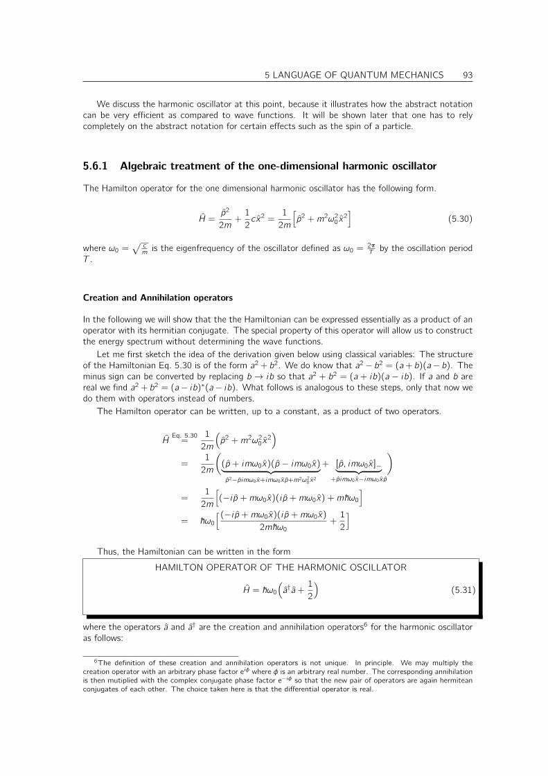
5 LANGUAGE OF QUANTUM MECHANICS 93
We discuss the harmonic oscillator at this point, because it illustrates how the abstract notationcan be very efficient as compared to wave functions. It will be shown later that one has to relycompletely on the abstract notation for certain effects such as the spin of a particle.
5.6.1 Algebraic treatment of the one-dimensional harmonic oscillator
The Hamilton operator for the one dimensional harmonic oscillator has the following form.
H =p2
2m+
1
2cx2 =
1
2m
[p2 +m2ω2
0 x2]
(5.30)
where ω0 =√
cm is the eigenfrequency of the oscillator defined as ω0 = 2π
T by the oscillation periodT .
Creation and Annihilation operators
In the following we will show that the the Hamiltonian can be expressed essentially as a product of anoperator with its hermitian conjugate. The special property of this operator will allow us to constructthe energy spectrum without determining the wave functions.
Let me first sketch the idea of the derivation given below using classical variables: The structureof the Hamiltonian Eq. 5.30 is of the form a2 + b2. We do know that a2− b2 = (a+ b)(a− b). Theminus sign can be converted by replacing b → ib so that a2 + b2 = (a + ib)(a − ib). If a and b arereal we find a2 + b2 = (a− ib)∗(a− ib). What follows is analogous to these steps, only that now wedo them with operators instead of numbers.
The Hamilton operator can be written, up to a constant, as a product of two operators.
HEq. 5.30
=1
2m
(p2 +m2ω2
0 x2)
=1
2m
((p + imω0x)(p − imω0x)︸ ︷︷ ︸p2−pimω0x+imω0x p+m2ω2
0 x2
+ [p, imω0x ]−︸ ︷︷ ︸+pimω0x−imω0x p
)
=1
2m
[(−i p +mω0x)(i p +mω0x) +m~ω0
]= ~ω0
[(−i p +mω0x)(i p +mω0x)
2m~ω0+
1
2
]Thus, the Hamiltonian can be written in the form
HAMILTON OPERATOR OF THE HARMONIC OSCILLATOR
H = ~ω0
(a†a +
1
2
)(5.31)
where the operators a and a† are the creation and annihilation operators6 for the harmonic oscillatoras follows:
6The definition of these creation and annihilation operators is not unique. In principle. We may multiply thecreation operator with an arbitrary phase factor eiφ where φ is an arbitrary real number. The corresponding annihilationis then mutiplied with the complex conjugate phase factor e−iφ so that the new pair of operators are again hermiteanconjugates of each other. The choice taken here is that the differential operator is real.

94 5 LANGUAGE OF QUANTUM MECHANICS
CREATION AND ANNIHILATION OPERATORS FOR THE HARMONIC OSCILLATOR
a =+i p +mω0x√
2m~ω0
(5.32)
a† =−i p +mω0x√
2m~ω0
(5.33)
We will call the operator a annihilation operator and a† creation operator.
We will see below that the operators create and annihilate excitations of the harmonic oscillator. Inquantum field theory, the excitations of the harmonic oscillator will be interpreted as particles, sothat a† and a create and annihilate particles. Note that a and a† are indeed hermitian conjugates ofeach other.
Spectrum of the harmonic oscillator
In the following we obtain the eigenvalue spectrum of the harmonic oscillator solely from abstractoperator equations. We will also find a first order differential equation for the ground state and arecursive equation for the higher states.
Let us evaluate the commutator algebra and let us in addition consider the anti-commutators aswell.
ANTI-COMMUTATOR
An anti-commutator [A, B]+ is defined as
[A, B]+ = AB + BA (5.34)
It looks like the commutator only with the sign reversed. In order to distinguish the commutatorclearly from the anticommutator, a “minus” sign is usually attached to the commutator [A,B] =[A,B]− = AB − BA. Another common notation is to use curly brackets for the anticommutator.
a†a =1
2~ω0mp2 −
i
2~
(px − x p
)+mω0
2~x2 =
1
~ω0H −
1
2(5.35)
aa† =1
2~ω0mp2 +
i
2~
(px − x p
)︸ ︷︷ ︸
=[p,x ]=~/i
+mω0
2~x2 =
1
~ω0H +
1
2(5.36)
[a†, a
]+
Eq. 5.36,5.35=
2H
~ω0(5.37)[
a†, a]−
Eq. 5.36,5.35= −1 (5.38)
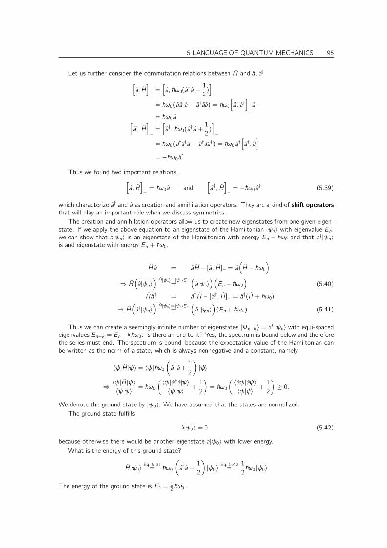
5 LANGUAGE OF QUANTUM MECHANICS 95
Let us further consider the commutation relations between H and a, a†[a, H
]−
=[a, ~ω0(a†a +
1
2)]−
= ~ω0(aa†a − a†aa) = ~ω0
[a, a†
]−a
= ~ω0a[a†, H
]−
=[a†, ~ω0(a†a +
1
2)]−
= ~ω0(a†a†a − a†aa†) = ~ω0a†[a†, a
]−
= −~ω0a†
Thus we found two important relations,[a, H
]−
= ~ω0a and[a†, H
]−
= −~ω0a†, (5.39)
which characterize a† and a as creation and annihilation operators. They are a kind of shift operatorsthat will play an important role when we discuss symmetries.
The creation and annihilation operators allow us to create new eigenstates from one given eigen-state. If we apply the above equation to an eigenstate of the Hamiltonian |ψn〉 with eigenvalue En,we can show that a|ψn〉 is an eigenstate of the Hamiltonian with energy En − ~ω0 and that a†|ψn〉is and eigenstate with energy En + ~ω0.
Ha = aH − [a, H]− = a(H − ~ω0
)⇒ H
(a|ψn〉
)H|ψn〉=|ψn〉En
=(a|ψn〉
)(En − ~ω0
)(5.40)
Ha† = a†H − [a†, H]− = a†(H + ~ω0)
⇒ H(a†|ψn〉
)H|ψn〉=|ψn〉En
=(a†|ψn〉
)(En + ~ω0) (5.41)
Thus we can create a seemingly infinite number of eigenstates |Ψn−k〉 = ak |ψn〉 with equi-spacedeigenvalues En−k = En−k~ω0. Is there an end to it? Yes, the spectrum is bound below and thereforethe series must end. The spectrum is bound, because the expectation value of the Hamiltonian canbe written as the norm of a state, which is always nonnegative and a constant, namely
〈ψ|H|ψ〉 = 〈ψ|~ω0
(a†a +
1
2
)|ψ〉
⇒〈ψ|H|ψ〉〈ψ|ψ〉 = ~ω0
(〈ψ|a†a|ψ〉〈ψ|ψ〉 +
1
2
)= ~ω0
(〈aψ|aψ〉〈ψ|ψ〉 +
1
2
)≥ 0.
We denote the ground state by |ψ0〉. We have assumed that the states are normalized.The ground state fulfills
a|ψ0〉 = 0 (5.42)
because otherwise there would be another eigenstate a|ψ0〉 with lower energy.What is the energy of this ground state?
H|ψ0〉Eq. 5.31
= ~ω0
(a†a +
1
2
)|ψ0〉
Eq. 5.42=
1
2~ω0|ψ0〉
The energy of the ground state is E0 = 12~ω0.

96 5 LANGUAGE OF QUANTUM MECHANICS
ENERGY SPECTRUM OF THE HARMONIC OSCILLATOR
The energy eigenvalue spectrum of the harmonic oscillator is equi-spaced
En = ~ω0(n +1
2) (5.43)
where n is a non-negative integer.
Again we observe that the ground state energy does not vanish, just asfor the particle in a box. The ground state energy is due to the so-calledzero-point vibrations or zero-point motion. It is not possible to removethat remaining energy out of the system. The origin of the zero-pointvibrations is Heisenberg’s uncertainty relation , which says that it is notpossible to find quantum mechanical system with a determined position andmomentum. That would be required for the classical system to be at rest.Can we observe the zero point vibration? We cannot observe it by removingthat energy, however if we compare the energy of an hydrogen molecule anda deuterium molecule, which have identical forces acting between the twoatoms. (Deuterium is an isotope of hydrogen with a mass about two timeslarger.) We find that the deuterium molecule is more stable by a few tenthsof an eV which is entirely due to the different zero-point energies. hω
hω
hω
hω
hω12
E
0
5.6.2 Wave functions of the harmonic oscillator
From the ground state all excited states can be constructed by repeatedly applying the creationoperator. However, we need to add normalization factor so that all states are properly normalized.
〈a†ψn|a†ψn〉 = 〈ψn|aa†|ψn〉Eq. 5.36
= 〈ψn|H
~ω+
1
2|ψn〉
Eq. 5.43= 〈ψn|ψn〉(n + 1)
⇒ |ψn+1〉 =1√n + 1
a†|ψn〉 (5.44)
〈aψn|aψn〉 = 〈ψn|a†a|ψn〉Eq. 5.35
= 〈ψn|H
~ω−
1
2|ψn〉
Eq. 5.43= 〈ψn|ψn〉n
⇒ |ψn−1〉 =1√na|ψn〉 (5.45)
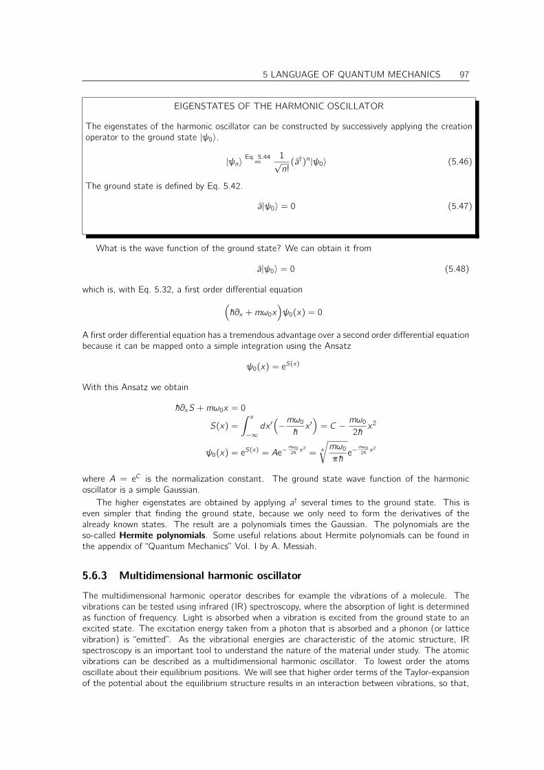
5 LANGUAGE OF QUANTUM MECHANICS 97
EIGENSTATES OF THE HARMONIC OSCILLATOR
The eigenstates of the harmonic oscillator can be constructed by successively applying the creationoperator to the ground state |ψ0〉.
|ψn〉Eq. 5.44
=1√n!
(a†)n|ψ0〉 (5.46)
The ground state is defined by Eq. 5.42.
a|ψ0〉 = 0 (5.47)
What is the wave function of the ground state? We can obtain it from
a|ψ0〉 = 0 (5.48)
which is, with Eq. 5.32, a first order differential equation(~∂x +mω0x
)ψ0(x) = 0
A first order differential equation has a tremendous advantage over a second order differential equationbecause it can be mapped onto a simple integration using the Ansatz
ψ0(x) = eS(x)
With this Ansatz we obtain
~∂xS +mω0x = 0
S(x) =
∫ x
−∞dx ′(−mω0
~x ′)
= C −mω0
2~x2
ψ0(x) = eS(x) = Ae−mω0
2~ x2
= 4
√mω0
π~e−
mω02~ x
2
where A = eC is the normalization constant. The ground state wave function of the harmonicoscillator is a simple Gaussian.
The higher eigenstates are obtained by applying a† several times to the ground state. This iseven simpler that finding the ground state, because we only need to form the derivatives of thealready known states. The result are a polynomials times the Gaussian. The polynomials are theso-called Hermite polynomials. Some useful relations about Hermite polynomials can be found inthe appendix of “Quantum Mechanics” Vol. I by A. Messiah.
5.6.3 Multidimensional harmonic oscillator
The multidimensional harmonic operator describes for example the vibrations of a molecule. Thevibrations can be tested using infrared (IR) spectroscopy, where the absorption of light is determinedas function of frequency. Light is absorbed when a vibration is excited from the ground state to anexcited state. The excitation energy taken from a photon that is absorbed and a phonon (or latticevibration) is “emitted”. As the vibrational energies are characteristic of the atomic structure, IRspectroscopy is an important tool to understand the nature of the material under study. The atomicvibrations can be described as a multidimensional harmonic oscillator. To lowest order the atomsoscillate about their equilibrium positions. We will see that higher order terms of the Taylor-expansionof the potential about the equilibrium structure results in an interaction between vibrations, so that,

98 5 LANGUAGE OF QUANTUM MECHANICS
in a crystal, we talk about phonon-phonon interactions. For further information on IR spectroscopysee Atkins[4]
The multidimensional oscillator has the Hamiltonian
H =∑i
p2i
2mi+
1
2
∑i ,j
xici ,j xj
It is always possible to transform this Hamiltonian onto a system of independent one-dimensionalharmonic oscillators shown as follows.
First we introduce new coordinates Xi =∑
j Ai ,j xj with a real matrix A.7 Per definition, thecanonical conjugate momentum P of X must fulfill the commutator relation8 9 [P , X] = ~
i , whichdetermines the momentum as Pi =
∑j A−1,>i ,j pj . Because we required the matrix A to be real, we
can replace A−1,> by A−1,†.
TRANSFORMATION OF MOMENTA UNDER A COORDINATE TRANSFORM
x ′i =∑j
Ai ,jxj ⇔ p′i =∑j
A−1,†i ,j pj (5.49)
The transformation matrix A is real. The transformation of momenta is chose such that the trans-formed coordinates and momenta obey the commutator relation [p′i , x
′j ] = ~
i δi ,j
We will use two such transformations in the following derivation. The first transformation is arescaling of the positions and momenta to get rid of the masses.
ξidef=√mi xi
πidef=
1√mipi
so that the Hamiltonian has the form
H =∑i
1
2π2i +
1
2
∑i ,j
ξi1√mici ,j
1√mj︸ ︷︷ ︸
Di ,j
ξj
7The generalization to complex transformations is at least problematic.8The transformation rules for the momenta can be obtained from classical physics as follows: Let us consider a
transformation of the coordinates.
xi = fi (~x′, t) ⇒ .
x i =∑j
∂fi
∂x ′j
.x′j +
∂fi
∂t
We already calculated the transformation for the velocities, which will be required in the followingNow we express the action by the old and the new coordinates
S[x(t)] =
∫dt L(~x,
.~x, t) =
∫dt L(~f (~x ′, t),
∑j
∂~f
∂x ′j
.x′j +
∂~f
∂t, t) =
∫dt L′(~x ′,
.~x′, t) = S[x ′(t)]
The momentum is defined related to the old and the new (primed) coordinates is
pi =∂L∂.x i
; and p′i =∂L′
∂.x′i
=∑j
∂L∂.x j
∂fj
∂x ′i=∑j
pj∂fj
∂x ′i
This provides the transformation rule for momenta for a given transformation of positions.9
[Pi , Xj ] =∑m,n
[A−1m,j pm, Ai ,n xn] =
∑m,n
A−1m,jAi ,n [pm, xn]︸ ︷︷ ︸
~i δm,n
=~i
∑m
Ai ,mA−1m,j︸ ︷︷ ︸
δi ,j
=~i

5 LANGUAGE OF QUANTUM MECHANICS 99
The matrix Di ,jdef= 1√
mici ,j
1√mj
is called dynamical matrix.We diagonalize the dynamical matrix so that∑
k
Di ,kUk,j = Ui ,jdj
the vector Uk,j for a given j is an eigenvector of D and dj is the corresponding eigenvalue. Weassume that the eigenvectors are normalized. Since the eigenvectors of a Hermitian matrix such asD are orthonormal, U is a unitary matrix.∑
k
U∗k,iUk,j = δi ,j
Especially for real matrices, the eigenvectors can be chosen to be real.10 This corresponds to atransformation, where the transformed coordinate axes point along the principal axes.11
Now we are ready to do the second transformation12
Xidef=∑j
U†i ,j ξj =∑j
U†i ,j√mj xj
Pidef=∑j
U†i ,j πj =∑j
U†i ,j1√mjpj
which yields13
H =∑i
(1
2P 2i +
1
2di X
2i
)Finally we use the method of separation of variables: We use the product Ansatz Ψ(X1, . . . , Xn) =∏n
i=1 φi(Xi), where each wave function φi(X) fulfills the Schrödinger equation for the one-dimensionalharmonic oscillator
Hi |φi 〉 = |φi 〉ei
Hi =1
2P 2i +
1
2di X
2i
There are of course many eigenvalues and eigenstates for each one-dimensional harmonic oscillator.For reasons of simplicity we suppress the corresponding index.
The eigenvalues for the multidimensional harmonic oscillator are
E =∑i
ei
and the wave functions are obtained as
Ψ(x1, . . . , xn) =
n∏i=1
φi
(∑k
Uik√mkxk
)10The eigenvectors are not necessarily real,which is important to know when using canned tools for the diago-
nalization. For real, hermitian matrices, however, the eigenvectors can be chosen real, because otherwise the formDi ,j =
∑k UikdkU
∗j,k would not be real.
11germ(principal axis) = Hauptachse12Note that (U†)−1† = U† since U is unitary.13
∑i
π2i =
∑i ,j,k
Ui ,jUi ,k Pj PkU=U∗
=∑i ,j,k
U∗i ,jUi ,k Pj Pk =∑j,k
Pj
(∑i
U†j,iUi ,k
)︸ ︷︷ ︸
δj,k
Pk =∑j
P 2j

100 5 LANGUAGE OF QUANTUM MECHANICS

Chapter 6
Representations
Fig. 6.1: Werner Heisen-berg, 1901-1976. Ger-man Physicist. Nobel price1933 in physics for the in-vention of Quantum Me-chanics, which he publishedonly 23 years old.
In the last section we introduced abstract states and operators thattransform them into each other. The only way to produce numbers isto evaluate scalar products and matrix elements. If we wish to representa state numerically, for example as wave function, we need to choose arepresentation. Choosing a representation in quantum mechanics is likechoosing a coordinate system for vectors. In quantum mechanical cal-culations, the choice of representations and the transformation betweenrepresentations is very important.
In this section we will learn about the matrix formulation of quantummechanics, where a state is represented by a vector and an operator isrepresented by a matrix. The only difficulty is that we need to deal withinfinitely many dimensions.
We will also see the connection to wave functions as used inSchrödinger’s wave-mechanical formulation of quantum mechanics,where states are functions in space. The wave function can be thoughtof as a vector with a continuous vector index.
6.1 Unity operator
Let us consider a complete set of states |ui 〉. Then we can express the unity operator as
1 =∑i ,j
|ui 〉Ki ,j 〈uj | (6.1)
where K is the inverse of the so-called overlap matrix O defined as Oi ,j = 〈ui |uj〉.∑k
Ki ,k〈uk |uj〉 = δi ,j (6.2)
101

102 6 REPRESENTATIONS
PROOF: we show that every state is mapped onto itself, if the unity operator in this form is applied to it.Every state |ψ〉 can be expressed as |ψ〉 =
∑i |ui〉ci if |ui〉 is complete.(∑
i ,j
|ui〉Ki ,j〈uj |)|ψ〉 =
(∑i ,j
|ui〉Ki ,j〈uj |)(∑
k
|uk〉ck)
=∑i ,k
|ui〉(∑
j
Ki ,j〈uj |uk〉)
︸ ︷︷ ︸=δi ,k Eq. 6.2
ck =∑i
|ui〉ci = |ψ〉
q.e.d.
If the set |ui 〉 is not only complete but also orthonormal, the overlap matrix O and its inverseK are unity matrices. Hence,
1 =∑i
|ui 〉〈ui |
for an orthonormal basis ui. In the following we assume |ui 〉 to be orthonormal.
6.2 Representation of a state
We can now express a state |ψ〉 in a certain representation. A representation is defined by a completebasis of orthonormal states |ui 〉. A state can be represented in a certain basis by multiplicationwith the unity operator
∑i |ui 〉〈ui |.
|ψ〉 =∑i
|ui 〉〈ui |ψ〉
Thus we can represent the state |ψ〉 by a vector ~ψ, where each vector component is a number,namely ψi = 〈ui |ψ〉. However, we need to specify the basis, namely the set |ui 〉. Compared toordinary vector algebra, the only uncommon points is that the vector has infinitely many componentsand that the vector components are complex numbers.
What we have done is similar to representing a vector ~r in three dimensions in a basis spanned bythree orthonormal basis vectors ~ex , ~ey , ~ez . We can write
~r = ~ex rx + ~ey ry + ~ez rz
Usually the vector ~r is then represented by its three components (rx , ry , rz). In order to know thevector ~r we need to know the choice of basis vectors ~ex , ~ey , ~ez and the vector components rx , ry , rzin this basis.
A special representation is the real space representation. Here the basis |r〉 is continuous. Thescalar products between states of the basis are defined as 〈r |r ′〉 = δ(r − r ′). Instead of a sum weneed to choose the integral. The unity operator has the form
1 =
∫d3r |r〉〈r |
Thus we obtain
|ψ〉 =
∫d3r |r〉〈r |ψ〉 =
∫d3r |r〉ψ(r)
so that we can represent the state by a function, the wave function ψ(r) = 〈r |ψ〉.
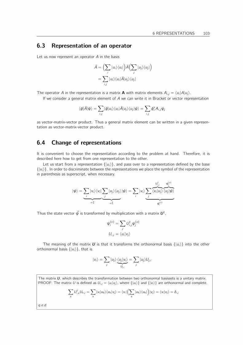
6 REPRESENTATIONS 103
6.3 Representation of an operator
Let us now represent an operator A in the basis
A =(∑
i
|ui 〉〈ui |)A(∑
j
|uj〉〈uj |)
=∑i ,j
|ui 〉〈ui |A|uj〉〈uj |
The operator A in the representation is a matrix A with matrix elements Ai ,j = 〈ui |A|uj〉.If we consider a general matrix element of A we can write it in Bracket or vector representation
〈φ|A|ψ〉 =∑i ,j
〈φ|ui 〉〈ui |A|uj〉〈uj |ψ〉 =∑i ,j
φ∗i Ai ,jψj
as vector-matrix-vector product. Thus a general matrix element can be written in a given represen-tation as vector-matrix-vector product.
6.4 Change of representations
It is convenient to choose the representation according to the problem at hand. Therefore, it isdescribed here how to get from one representation to the other.
Let us start from a representation |ui 〉, and pass over to a representation defined by the base|vi 〉. In order to discriminate between the representations we place the symbol of the representationin parenthesis as superscript, when necessary.
|ψ〉 =∑i
|vi 〉〈vi |︸ ︷︷ ︸=1
∑j
|uj〉〈uj |︸ ︷︷ ︸=1
|ψ〉 =∑i
|vi 〉∑j
U†i ,j︷ ︸︸ ︷〈vi |uj〉
ψ(u)j︷ ︸︸ ︷
〈uj |ψ〉︸ ︷︷ ︸ψ
(v)i
Thus the state vector ~ψ is transformed by multiplication with a matrix U†,
ψ(v)i =
∑j
U†i ,jψ(u)j
Ui ,j = 〈ui |vj〉
The meaning of the matrix U is that it transforms the orthonormal basis |ui 〉 into the otherorthonormal basis |vi 〉, that is
|vi 〉 =∑j
|uj〉 〈uj |vi 〉︸ ︷︷ ︸Uj,i
=∑j
|uj〉Uj,i
The matrix U, which describes the transformation between two orthonormal basissets is a unitary matrix.PROOF: The matrix U is defined as Ui ,j = 〈ui |vj〉, where |ui〉 and |vi〉 are orthonormal and complete.∑
k
U†i ,kUk,j =∑k
〈vi |uk〉〈uk |vj〉 = 〈vi |(∑
k
|uk〉〈uk |)|vj〉 = 〈vi |vj〉 = δi ,j
q.e.d.

104 6 REPRESENTATIONS
The transformation of matrix elements proceeds similar and we obtain
〈vi |A|vj 〉 = 〈vi |(∑
k
|uk〉〈uk |)A(∑
l
|ul〉〈ul |)|vj〉
A(v)i ,j =
∑k,l
U†i ,kA(u)k,l Ul ,j
Let us summarize the transformation rules:
CHANGE OF REPRESENTATION
Under a change from one orthonormal basis to another, the vector components of a state and thematrix elements transform as
ψ(v)i =
∑j
U†i ,jψ(u)j (6.3)
A(v)i ,j =
∑k,l
U†i ,kA(u)k,l Ul ,j (6.4)
where
Ui ,j = 〈ui |vj〉 (6.5)
is a unitary matrix.
6.5 From bra’s and ket’s to wave functions
6.5.1 Real-space representation
Now we have learned to deal with abstract states and with wave functions. What is missing is howto translate the expressions from one formulation to the other. While the connection is better shownin the context of representation theory discussed later in chapter 6, I will show here already the mainarguments.
The connection between the two formulations lies in
Ψ(x)def=〈x |Ψ〉 (6.6)
where the states |x〉 form a complete set of states. Note, however, that the states |x〉 are notelements of the Hilbert space, but lie in the extended Hilbert space.
Similarly, the meaning of of the somewhat sloppy expression Aψ(x), where A is an arbitraryoperator, is as follows
Aψ(x)def=〈x |A|ψ〉
The states |x〉 obey the conditions:
x |x〉 = |x〉x eigenvalue equation (6.7)
〈x |x ′〉 = δ(x − x ′) orthonormality (6.8)
1 =
∫dx |x〉〈x | completeness (6.9)
The second equation, Eq. 6.8, shows that the wave function related to the state |x0〉, definedaccording to Eq. 6.6, is a δ-function located at position x0.

6 REPRESENTATIONS 105
Position and momentum operators have the form1
x =
∫dx |x〉x〈x | (6.10)
p =
∫dx |x〉
~i∂x 〈x | (6.11)
The Schrödinger equation has the following form in the abstract notation and the wave functionnotation. (
p2
2m+ v(x)
)|ψ〉 = |Ψ〉E (6.12)(
−~2
2m∂2x + v(x)
)ψ(x) = ψ(x)E (6.13)
The two above versions of the Schrödinger equations are mathematically correct. However, anequation like the following is, strictly speaking, meaningless[
−~2
2m∂2x + v(x)
]|ψ〉 = |ψ〉E
because a function in space is multiplied with a abstract state. Nevertheless, such a notation is oftenused in practice.
The difficult steps in the derivation of the above expression Eq. 6.13 from Eq. 6.12 are
1. to represent a function of an operator
v(x)|x〉 Eq. 5.29= |x〉v(x)
⇒ v(x) = v(x)
∫dx |x〉〈x |︸ ︷︷ ︸
1
=
∫dx |x〉v(x)〈x |
1 We first show that the first equation Eq. 6.10 holds:
xEq. 6.9
= x
∫dx |x〉〈x |︸ ︷︷ ︸
1
=
∫dx x |x〉︸︷︷︸
|x〉x
〈x | Eq. 6.7=
∫dx |x〉x〈x |
Now we show that the second equation Eq. 6.11 holds: The momentum operator is defined as that operator thathas a commutator [p, x ] = ~
i. Thus we need to show that the commutator has the correct value.
[p, x ]Eq. 5.25
= px − x pEq. 6.11
=
∫dx |x〉
~i∂x 〈x |
∫dx ′ |x ′〉x ′〈x ′| −
∫dx ′ |x ′〉x ′〈x ′|
∫dx |x〉
~i∂x 〈x |
=
∫dx
∫dx ′
|x〉~i ∂x 〈x |x ′〉︸ ︷︷ ︸δ(x−x ′)
x ′〈x ′| − |x ′〉x ′ 〈x ′|x〉︸ ︷︷ ︸δ(x−x ′)
~i∂x 〈x |
=
∫dx
(|x〉~i∂xx〈x | − |x〉x
~i∂x 〈x |
)=
∫dx |x〉
( ~i∂xx︸ ︷︷ ︸
~i +x ~i ∂x
−x~i∂x
)〈x | =
~i

106 6 REPRESENTATIONS
2. to square the momentum operator
p2 Eq. 6.11=
(∫dx |x〉
~i∂x 〈x |
)(∫dx ′ |x ′〉
~i∂x ′〈x ′|
)
=
∫dx |x〉
~i∂x
∫ dx ′ 〈x |x ′〉︸ ︷︷ ︸δ(x−x ′)
~i∂x ′〈x ′|
=
∫dx |x〉
~i∂x
(~i∂x 〈x |
)=
∫dx |x〉(−~2∂2
x )〈x |
6.5.2 Momentum representation
What are the momentum eigenstates? We start from the eigenvalue equation for the momentumoperator, which defines the momentum eigenstates |p〉 up to a constant.
p|p〉 = |p〉p eigenvalue equation (6.14)
We would like to know the momentum eigenstates as wave functions: With the help of Eq. 6.11we obtain an eigenvalue equation for 〈x |p〉.∫
dx |x〉~i∂x 〈x |p〉
Eq. 6.14=
∫dx |x〉〈x |p〉p
Now, we exploit that the kets |x〉 are linear independent. This implies that the coefficients for thekets |x〉 must be pairwise identical.
⇒~i∂x 〈x |p〉 = 〈x |p〉p
This is a differential equation with constant coefficients for the function f (x)def=〈x |p〉, which can be
solved with the exponential ansatz. As solution, one obtains a simple plane wave
〈x |p〉 = ei~ px (6.15)
One should be careful not to write 〈x |p〉 = p(x) even though this is formally correct: One couldeasily mistake it for a function that expresses the momentum as function of position.
Note that the prefactor of the wave function can be chosen in different ways. In our notation theorthonormality condition and the representation of the unity operator are.
ORTHONORMALITY AND COMPLETENESS OF MOMENTUM EIGENSTATES
〈p|p′〉 = 2π~ δ(p − p′) orthonormality (6.16)
1 =
∫dp
2π~|p〉〈p| completeness (6.17)
In many textbooks, the momentum eigenstates are defined as |p〉 = 1√2π~e
i~ px . That is they
are normalized differently. Our notation has the advantage that the factors 1√2π~ do not appear in
the real space wave function corresponding to the momentum eigenstate. On the other hand, ournotation requires the factors 2π~ in the normalization condition Eq. 6.16 and the representation ofthe unit operator, Eq. 6.17, which do not occur in the other notation.

6 REPRESENTATIONS 107
6.5.3 Orthonormality condition of momentum eigenstates (Home study)
Here, we derive the normalization condition of the momentum eigenstates, namely Eq. 6.16. We usethe expression Eq. 6.15 for the real space wave function of a momentum eigenstate.
〈p|p′〉 = 〈p|
1︷ ︸︸ ︷∫ ∞−∞
dx |x〉〈x | |p′〉 =
∫ ∞−∞
dx 〈p|x〉〈x |p′〉 =
∫ ∞−∞
dx ei~ (p−p′)x (6.18)
This expression is awkward, because it contains an integral that does not even converge, if thebounds of the integral are at infinity. Therefore, we have to play a common trick to make the integralconverge anyway2: We multiply the integrand with a function, namely e−λ|x |, that attenuates theoscillations for large arguments, i.e. at ±∞. For each value of λ, the integral is well defined. As λapproaches zero, the function e−λ|x | approaches 1. Hence, we recover the original integral Eq. 6.18in the limit λ→ 0.
〈p|p′〉 = limλ→0+
∫ ∞−∞
dx e( i~ (p−p′)xe−λ|x |
= limλ→0
(∫ 0
−∞dx e( i~ (p−p′)+λ)x +
∫ ∞0
dx e( i~ (p−p′)−λ)x
)= lim
λ→0
((i
~(p − p′) + λ
)−1
−(i
~(p − p′)− λ
)−1)
= limλ→0
−2λ−1~2 (p − p′)2 − λ2
= 2~ limλ→0
~λ(p − p′)2 + ~2λ2
(6.19)
The function in the limes has the form of a Lorentzian. A Lorentzian is defined as L(x) =1π
Γ/2(x−x0)2+(Γ/2)2 . The Lorentzian has a peak at x0 and a width related to Γ. The Lorentzian has the
−4
0.1
0.2
0.3
0.4
0.5
0.6
0.7
−2 0 2 4 0
Fig. 6.2: Lorentzian with width Γ = 1
form of a spectral line in an absorption spectrum.We recognize already that the function in Eq. 6.19 vanishes in the limit for p 6= p′ and that it
diverges for p = p′, which suggests that the limes could be a delta function. What needs to be shownis that the integral over p is equal to a well-defined constant.
2The background is the theory of Distributions, which are generalizations of functions such as the delta functionof Dirac. See [25]. Editor: In the first line we interchange the limit and the integral. Is this legitimate?

108 6 REPRESENTATIONS
We use the integral formula taken from Bronstein[26]∫dx
1
x2 + a2=
1
aatan(
x
a)
Thus we obtain∫ ∞−∞
dp 〈p|p′〉 Eq. 6.19= 2~ lim
λ→0
[atan(
p − p′
~λ)
]∞−∞
= 2~
atan(∞)︸ ︷︷ ︸π/2
− atan(−∞)︸ ︷︷ ︸−π/2
= 2π~
Since a function that integrates to one, but vanishes everywhere except one point is a delta function3
, we can directly express the scalar product as
〈p|p′〉 = 2π~ δ(p − p′)
which proves Eq. 6.16.Now it is a simple matter to determine the unity operator in momentum representation as given
in Eq. 6.17. The form of the unity operator can be verified by showing that it does not change thestate to which it is applied. It is sufficient to show this for an arbitrary state from a complete set ofstates, which we choose to be the momentum eigenstates |p〉.
Due to the superposition principle, it holds for any state if it holds for a complete set of statessuch as |p〉. The identity is shown as follows:
1|p〉 Eq. 6.17=
∫dp′
2π~|p′〉〈p′|p〉 Eq. 6.16
=
∫dp′
2π~|p′〉2π~δ(p − p′) = |p〉
6.6 Application: Two-state system
After the harmonic oscillator, we learn here about the second most important model in quantummechanics, the two-state system. The two-state system is useful as a model for any system whereonly the ground state and the first excited state is accessible. At low temperatures for example, itmay happen that we only have to consider the lowest two states. There are also systems that onlyhave two states. We will learn that the spin of an electron, which is the rotation of an electron aboutitself, can only have two states namely a clock-wise and a counter-clock wise rotation about an axiswith a well defined absolute value of the angular momentum.
We denote the two states with the symbols |ψ0〉 and |ψ1〉. |ψ0〉 is the ground state of the systemand |ψ1〉 is the first excited state.
Let us assume that they are eigenstates of the Hamilton operator with eigenvalues ε0 for theground state and ε1 for the excited state. Therefore,
H|ψ0〉 = |ψ0〉ε0
H|ψ1〉 = |ψ1〉ε1 (6.20)
We will see later that we can always choose the eigenstates to be orthonormal, that is
〈ψi |ψj 〉 = δi ,j
We can now express the Hamilton operator in the basis of its eigenstates, so that it is representedby a matrix (
〈ψ0|H|ψ0〉 〈ψ0|H|ψ1〉〈ψ1|H|ψ0〉 〈ψ1|H|ψ1〉
)Eq. 6.20
=
(ε0 0
0 ε1
)=: H
3This conclusion is not entirely strict because there are also distributions (functions) that are zero everywhere andintegrate to zero. An example is the derivative of the delta function. An admixture of these functions cannot beexcluded.

6 REPRESENTATIONS 109
The Hamilton operator has the form
H =
1∑i ,j=0
|ψi 〉Hi ,j 〈ψj | = |ψ0〉ε0〈ψ0|+ |ψ1〉ε1〈ψ1| (6.21)
Hence we can write the Hamilton matrix H.
H =
(ε0 0
0 ε1
)=ε0 + ε1
2
(1 0
0 1
)+ε1 − ε0
2
(−1 0
0 1
)
Without loss of generality, we can choose the energy zero to be equal with ε0+ε1
2 , the mean value ofthe two energies, which deletes the first term in the above equation. Furthermore we introduce thefrequency ω0 via the excitation energy
~ω0def=ε1 − ε0
so that
H =1
2~ω0
(−1 0
0 1
)
Now we would like to create ladder operators just as for the harmonic oscillator they are definedby
a|ψ0〉 = |∅〉a|ψ1〉 = |ψ0〉 (6.22)
Note here that |∅〉 6= |ψ0〉! |∅〉 is the zero-state and is associated with a wave function that is zeroeverywhere in space. |ψ0〉 on the other hand is the ground state.
Let us evaluate a in the representation (|ψ0〉, |ψ1〉)(〈ψ0|a|ψ0〉 〈ψ0|a|ψ1〉〈ψ1|a|ψ0〉 〈ψ1|a|ψ1〉
)Eq. 6.22
=
(0 1
0 0
)
The states are orthonormal. We will later see that eigenstates of any hermitian operator (such asthe Hamiltonian) to different eigenvalues are always orthogonal.
We can now evaluate the matrix elements of a† as(〈ψ0|a†|ψ0〉 〈ψ0|a†|ψ1〉〈ψ1|a†|ψ0〉 〈ψ1|a†|ψ1〉
)=
(〈ψ0|a|ψ0〉∗ 〈ψ1|a|ψ0〉∗
〈ψ0|a|ψ1〉∗ 〈ψ1|a|ψ1〉∗
)=
(0 0
1 0
)
Let us now investigate the commutator relations: We start working out the products of the ladderoperators. We can use the matrix notation, if we stay in the representation of eigenstates.
a†a =
(0 0
0 1
); aa† =
(1 0
0 0
)
a2 =
(0 0
0 0
)=∅ ; a†2 =
(0 0
0 0
)= ∅
Hence we can write the Hamiltonian as
H =1
2~ω0[a†, a]−=
1
2~ω0
(−1 0
0 1
)

110 6 REPRESENTATIONS
while the anti-commutator4 is a constant
[a, a†]+ = 1
[a, a]+ = ∅[a†, a†]+ = ∅
Note here, that the commutator relations are similar to those of the harmonic oscillator as seen inEq. 5.38 only that commutators and anti-commutators are interchanged. This will be important ifwe pass to a many particle description of Fermions such as the electron.
6.6.1 Pauli Matrices
It can be shown that all matrices in two dimensional space can be expressed in terms of 4 Hermitianmatrices, the three so-called Pauli matrices and the unity operator. Pauli matrices play an importantrole for the description of spin and in general for certain particles called Fermions. Therefore, weshall introduce them here. Some useful expressions that facilitate working with Pauli matrices areprovided in App. R.
We can now look for the most general form of an observable in the space spanned by the twostates. The most general Hermitian two-by-two matrix has the form
A =
(a b + ic
b − ic d
)which can be expressed in the form
A =a + d
2
(1 0
0 1
)+ b
(0 1
1 0
)− c
(0 −ii 0
)+a − d
2
(1 0
0 −1
)
=a + d
2+ bσx − cσy +
a − d2
σz
with real coefficients and the so-called Pauli matrices σx , σy and σz .
PAULI MATRICES
σx =
(0 1
1 0
); σy =
(0 −ii 0
); σz =
(1 0
0 −1
). (6.23)
The multiplication table, commutators and anti-commutators of Pauli matrices are derived inApp. R. Since these relations will be useful for what follows I recommend to go through that appendixat this point.
While we started with observables, that is with hermitian matrices, it can be shown that any 2×2matrix, and not only Hermitian matrices, can be expressed as superposition of the identity and thePauli matrices with complex coefficients.
As an example, the ladder operators have the form
a =1
2(σx − i σy ); a† =
1
2(σx + i σy )
and the Hamilton operator can be written as
H =1
2~ωσz (6.24)
4See Eq. 5.34 on p. 94 for a definition of the anti-commutator

6 REPRESENTATIONS 111
6.6.2 Excursion: The Fermionic harmonic oscillator (Home study)
This section is a fun chapter. There is no harm if you skip to the next section, at least for themoment. If you are still with me, lean back and enjoy! We will get a glimpse into the field ofsuper-symmetry, which plays a role in elementary particle physics.
Super-symmetry is important because of the zero point motion. We will see later that whenwe quantize fields the zero point motion of the harmonic oscillator results in an infinite energyeven for free space. At first this does not seem like a big problem, because we can always add acompensating energy. However, the theory of general relativity says that energy, which is a type ofmass in this theory, distorts space and therefore results in gravitational forces. So, when we consideralso gravitational forces, the zero-point energy is observable and we cannot simply get rid of it.One attempt to get rid of the zero-point energy is to introduce for every harmonic oscillator also acorresponding two-state system, so that their positive and negative zero point motions cancel outexactly. This is the basic idea of super-symmetry. We will later talk about particles, Bosons andFermions, where the Fermions are particles that are represented by a two-state system in each pointin space and Bosons are particles that are represented by harmonic oscillators. But now we havealready gone way beyond what we learned sofar.
What we try to do here is to develop the two-state system analogously to the harmonic oscillator.In the two-state system and in the harmonic oscillator we used creation and annihilation operatorsto construct the eigenvalue spectrum. We have seen that a lot is similar but that commutators andanti-commutators interchange their role.
Here we follow up on that analogy between two-state systems and the harmonic oscillator anddevelop what is called the Fermionic harmonic oscillator. The main question we will ask is: What arethe coordinate and momentum operators that describe the two-state system.
We build the momenta and position operators from odd and even combinations of the creationand annihilation operators roughly analogous to the ordinary harmonic oscillator.
χ =
√~2
(a† + a)
π = i
√~2
(a† − a)
Both are Hermitian operatorsLet us work out the product table
χ2 =~2
; π2 =~2
; πχ = +i~2σz ; χπ = −i
~2σz ;
in order to derive the commutation and anti-commutation relations
[χ, χ]+ = ~ [χ, χ]− = 0
[π, π]+ = ~ [π, π]− = 0
[π, χ]+ = 0 [π, χ]− = i~σz
Thus we can express the Hamilton operator in the form
HEq. 6.24
=~ω2σz =
−iω2
[π, χ]−[π,χ]+=0
= iωχπ
Now we see the analogy in full glory. It seems that all we need to do is to interchange plus andminus signs.

112 6 REPRESENTATIONS
harmonic oscillator two-state system
(anti-)commutators [a, a†]− = 1 [a, a†]+ = 1
[a, a]− = [a†, a†]− = 0 [a, a]+ = [a†, a†]+ = 0
Hamilton operator H = 12~ω0[a†, a]+ H = 1
2~ω0[a†, a]−
momentum p = im~ω0(a†+a)√2m~ω0
π = i√~2 (a† − a)
position x = ~(a†+a)√2m~ω0
χ =√~2 (a† + a)
annihilator a = i p+mωx√2m~ω0
a = i π+χ√2~
creator a = −i p+mωx√2m~ω0
a = −i π+χ√2~
(anti)-commutators [p, x ]− = ~i [π, χ]+ = 0
[p, p]− = [x , x ]− = 0 [π, π]+ = [χ, χ]+ = ~
Hamilton operator p2
2m +mω2x2 iωχπ
The classical limit is really funny. If we let ~ go to zero, we find that interchanging π’s and χ’s ina product still changes its sign. This is the so-called Grassmann algebra. In the Grassmann algebrawe work with numbers, but any interchange of two numbers changes the sign of the product.
Why do we call this two-state system a harmonic oscillator? The regular harmonic oscillator hasthe property that the classical system has exactly one frequency. Let us therefore derive the classicalHamilton equations.
.χ =
∂H
∂π= −iωχ⇒ χ(t) = e−iωtA
.π = −
∂H
∂χ= −iωπ ⇒ π(t) = e−iωtB
(Note, that there seems to be a sign error in the first of the two last equation. This is not so, becausewe have to interchange χ and π in the Hamiltonian before we can form the derivative. Due to theanti-commutation relation for χ and π, this introduces a sign change.) Thus the “positions” χ andmomenta perform oscillations with a single frequency just as the regular harmonic oscillator.

Chapter 7
Measurements
Fig. 7.1: Niels Bohr, 1892-1987. Danish Physicist.Nobel price 1922 for his in-vestigations of the struc-ture of atoms and theradiation emanating fromthem.
The main new feature of quantum mechanics as discussed so far wasto replace particles by wave packets. Thus make the transition from aclassical particle theory to a, still classical, field theory. The quantummechanical measurement process is what is really puzzling about quan-tum mechanics. The rules are fairly clear, but there is still an ongoingdiscussion about its meaning.
In classical mechanics, measurable quantities are associated withfunctions A(q, p) of the coordinates and momenta– or alternatively thevelocities–in configuration space. A measurable quantity for a state isobtained by evaluating the value of the function A for this state. Inquantum mechanics a measurable quantity is associated with an Her-mitian operator.
7.1 Expectation values
Quantum theory does not predict the outcome of an experiment withcertainty. However, it predicts the mean value of a measurable quantitywhen the experiment is repeated sufficiently often. This is less of alimitation than it seems, because we may very well measure the spread ofthe measured values. Hence, we can predict under which circumstancesour prediction will be certain.
The mean value of a measured quantity is called expectation value.The expectation value of an operator A and a quantum mechanical state |ψ〉 is obtained as
〈A〉 =〈ψ|A|ψ〉〈ψ|ψ〉 (7.1)
In the following we assume that the state |ψ〉 is normalized, so that we can express the expectationvalue simply as
〈A〉 〈ψ|ψ〉=1= 〈ψ|A|ψ〉
7.2 Certain measurements
If a state predicts a sharp value of an observable A, the state is an eigenstate of A.
113

114 7 MEASUREMENTS
Let us consider the square variation1 σ2 of an observable from its expectation value in somestate. Given a state |ψ〉 we define the deviation ∆A from the expectation value of that state.
∆Adef= A− 〈ψ|A|ψ〉1 (7.2)
Note that ∆A describes one operator. The operator depends on the state |ψ〉. The expectation valuein Eq. 7.2 is considered a fixed number. The square deviation is then the expectation value of (∆A)2.Let us work out the expectation value of the square deviation
〈ψ|(∆A)2|ψ〉 =⟨ψ|(A− 〈A〉
)2 |ψ⟩
=
⟨ψ|
(A−
〈ψ|A|ψ〉〈ψ|ψ〉
)2
|ψ
⟩
= 〈ψ|A2|ψ〉 − 2〈ψ|A|ψ〉〈ψ|A|ψ〉〈ψ|ψ〉 + 〈ψ|ψ〉
(〈ψ|A|ψ〉〈ψ|ψ〉
)2
〈ψ|(∆A)2|ψ〉〈ψ|ψ〉 =
〈ψ|A2|ψ〉〈ψ|ψ〉 −
(〈ψ|A|ψ〉〈ψ|ψ〉
)2
(7.3)
of a measurable quantity in an experiment for a given wave function.Using the expression Eq. 7.1 for the expectation value we find
〈(∆A)2〉 Eq. 7.3= 〈A2〉 − 〈A〉2
This result reminds strongly of the classical expression for the square deviation σ2A of a quantity A.
We consider here an experiment, which contains some randomness. The measurement can produceany of the possible values ai of A. The frequency of the outcome ai is Pi , which is the number oftimes ai was the measured result relative to the total number of measurements. The frequency Pican be interpreted as probability of the outcome ai . The mean value of the measured quantity A is
〈A〉def=∑i
Piai
and the square deviation is
σ2A = 〈(A− 〈A〉)2〉 =
∑i
Pi(ai − 〈A〉)2 =∑i
Pi(a2i − 2ai 〈A〉+ 〈A〉2)
=∑i
Pia2i︸ ︷︷ ︸
〈A2〉
−2〈A〉∑i
Piai︸ ︷︷ ︸〈A〉
+〈A〉2)
= 〈A2〉 − 〈A〉2
After this little detour we return back to quantum mechanics.
Since the operator is Hermitian – it corresponds to a measurable quantity –, the condition for acertain prediction without spread is
〈(∆A)2〉 = 0
which implies
〈(∆A)2〉 Eq. 7.3= 〈ψ|A2ψ〉〈ψ|ψ〉 − 〈Aψ|ψ〉2
⇒ 〈Aψ|Aψ〉︸ ︷︷ ︸〈φ|φ〉
〈ψ|ψ〉 = 〈Aψ|ψ〉︸ ︷︷ ︸〈φ|ψ〉
〈ψ|Aψ〉︸ ︷︷ ︸〈ψ|φ〉
1germ: Quadratische Abweichung
7 MEASUREMENTS 115
Let us introduce |φ〉 def= A|ψ〉. Schwarz’ inequality, which is derived below in 7.4, says that forany two states |φ〉 and |ψ〉 the inequality
〈φ|φ〉〈ψ|ψ〉 − 〈φ|ψ〉〈ψ|φ〉Eq. 7.4
≥ 0
holds and that the equal sign holds, if the two states |ψ〉 and |φ〉 are linear dependent, i.e. |φ〉 = |ψ〉a,with some proportionality factor a.
For our problem with 〈(∆A)2〉 = 0, Schwarz’ inequality implies
A|ψ〉 = |ψ〉a
We call such an equation an eigenvalue equation. The state |ψ〉 is called eigenstate, and the valuea is called an eigenvalue. Thus we have shown that a sharp measurement is only possible for aneigenstate of the corresponding operator.
7.2.1 Schwarz’ inequality
Let us now derive Schwarz’ inequality we used before.
SCHWARZ’ INEQUALITY
Schwarz’ inequality says that for two arbitrary states |φ〉 and |ψ〉
〈φ|φ〉〈ψ|ψ〉 − 〈φ|ψ〉〈ψ|φ〉 ≥ 0 (7.4)
and that the equality holds only when |φ〉 and |ψ〉 are linearly dependent, i.e. if |φ〉 = |ψ〉a with some(complex) proportionality constant a.
The essence of Schwarz inequality is that a vector becomes shorter if we project something outof it. The above relation can be written as
〈ψ|(
1− |φ〉1
〈φ|φ〉 〈φ|)|ψ〉
Eq. 7.4
≥ 0
In order to grasp the meaning of Schwarz’ inequality consider regular vectors instead of quantummechanical states. For regular vectors Schwarz inequality says
~a2~b2 − (~a~b)2 ≥ 0
Dividing this expression by the squared length of the two vectors yields
1−
(~a ~b
|~a||~b|
)2
= 1− cos2(α) = sin2(α) ≥ 0
where α is the angle between the two vectors. Clearly, the squared sinus is always positive and itvanishes for an angle of 0 and 180, that is for parallel or antiparallel vectors. The analogy withregular vectors may be instructive in the proof of Schwarz’ inequality for quantum mechanical states.
The proof of Schwarz inequality goes as follows:

116 7 MEASUREMENTS
PROOF of Schwarz inequality Eq. 7.4: Let us say we have two states |ψ〉 and |φ〉. Out of the two states,we construct one, |δ〉 = |φ〉 〈ψ|ψ〉 − |ψ〉〈ψ|φ〉, that is orthogonal to |ψ〉. We express |φ〉 as
|φ〉 =[|δ〉+ |ψ〉 〈ψ|φ〉
] 1
〈ψ|ψ〉
and evaluate its norm exploiting the orthogonality 〈ψ|δ〉 = 0
〈φ|φ〉 =[〈δ|δ〉+ 〈φ|ψ〉〈ψ|ψ〉〈ψ|φ〉
] 1
〈ψ|ψ〉2
⇒ 〈φ|φ〉〈ψ|ψ〉 − 〈φ|ψ〉〈ψ|φ〉 =〈δ|δ〉〈ψ|ψ〉
|δ><ψ|ψ>
<ψ|ψ>|ψ><ψ|
|φ>
|ψ>
|ϕ>
1. Since the norm of every state is positive or zero, the right hand side is positive or zero.
2. The right hand side vanishes, when |δ〉 = 0. In that case, however, we find from the equation defining|δ〉 that
|φ〉 = |ψ〉 〈ψ|φ〉〈ψ|ψ〉
Hence |φ〉 and |ψ〉 are linearly dependent if the equal sign holds.
q.e.d.
7.3 Eigenstates
We have learned that the uncertainty of a measurement vanishes, if the state is an eigenstateof the operator corresponding to the measured quantity. Eigenstates play an important role inmeasurements.
There are a few important points to know about eigenstates:
1.The eigenvalues of a Hermitian operator are real.
PROOF: Let ψ be an eigenstate of the Hermitian operator A with eigenvalue a.
〈ψ|ψ〉a = 〈ψ|A|ψ〉 = 〈ψ|A†|ψ〉∗ A=A†= 〈ψ|A|ψ〉∗ = 〈ψ|ψ〉∗a∗
Because the norm of a state is real, we find that the eigenvalue a = a∗ is real, too.q.e.d
2.The eigenstates of a Hermitian operator with different eigenvalues are orthogonal.

7 MEASUREMENTS 117
PROOF: Let us consider two eigenstates |ψ1〉 and ψ2〉 of a Hermitian operator A with different eigen-values a1 and a2.Because A is Hermitian we obtain
0 = 〈φ|A− A†|ψ〉
We continue by using the eigenvalue equations A|ψ1〉 = |ψ1〉a1 and A|ψ2〉 = |ψ2〉a2.
0 = 〈ψ1|A− A†|ψ2〉= 〈ψ1|A|ψ2〉 − 〈ψ2|A|ψ1〉∗
= 〈ψ1|ψ2〉a2 − 〈ψ2|ψ1〉∗a∗1= 〈ψ1|ψ2〉[a2 − a1]
(Note that a∗1 = a1, since A is Hermitian.) If the eigenvalues are different this equation can only befulfilled if the scalar product vanishes, thus the two eigenstates are orthogonal.q.e.d.
3.
Any linear combination of eigenstates of an operator with the same eigenvalue is itself aneigenstate with this eigenvalue.
PROOF: We start with two eigenstates to A with the same eigenvalue a
A[|ψ1〉c1 + |ψ2〉c2] = [A|ψ1〉c1 + A|ψ2〉c2] = [|ψ1〉ac1 + |ψ2〉ac2] =
= [|ψ1〉c1 + |ψ2〉c2]a
q.e.d.
4.
The eigenstates to the same eigenvalue can be orthogonalized. The number of orthogonaleigenstates for a given eigenvalue is called the degeneracy of that eigenvalue.
PROOF: This is a trivial statement, because any set of states can be orthogonalized. Here we showa procedure to do this in practice. The method is called Gram-Schmidt orthogonalization.We start out from a set of states |ψi〉 and orthogonalize them recursively. The resulting states |φi〉will not only be orthogonalized but also normalized, so that 〈φi |φj〉 = δi ,j .
|ξn〉 = |ψn〉 −n−1∑j=1
|φj〉〈φj |ψn〉
|φn〉 = |ξn〉1√ξn|ξn〉
In a first step, the orthogonalization step, we produce the states |ξn〉. Only those states |φn〉 are requiredthat have already been constructed. We can assume that the states |φj〉 are normalized, because, inthe second step, the normalization step, the orthonormalized state |φ〉 is obtained by scaling |ξn〉. Therecursive equation can produce a zero state |ξn〉 = 0, which produces a divide-by-zero in the next step.When this happens |ψn〉 is linearly dependent to the other states and must be excluded from the set.Thus, the orthogonal set |φj〉 may have less elements than the initial set |ψi〉. q.e.d.
The set of all eigenvalues of an operator A is called the spectrum of A. The spectrum can be partlydiscrete and partly continuous. We denote the eigenstates with discrete eigenvalues with in integerindex |φi 〉 and those from the continuous spectrum |φα〉 with a continuous index α.

118 7 MEASUREMENTS
We normalize the states that
〈φi |φj〉 = δi ,j
〈φα|φα′〉 = δ(α− α′)〈φi |φα〉 = 0
If the orthogonal system of eigenstates is complete, that is every state |ψ〉 can be represented assuperposition of eigenstates φi ,
|ψ〉 =∑i
|φi 〉ci +
∫dα|φα〉cα
then the Hermitian operator is called an observable. The coefficients are ci = 〈φi |ψ〉 and cα =〈φα|ψ〉.
Important Note! In the following we will often use the sum alone even if the eigenvalue spectrummay be completely or partly continuous. In this case, we always imply summation over all states ofthe discrete part of the spectrum and integration over all states from the continuous spectrum.
We have already made contact with operators with discrete and with continuous eigenvaluespectra. The Hamiltonian of the harmonic oscillator has a purely discrete eigenvalue spectrum. TheHamiltonian for the free particle on the other hand has a purely continuous eigenvalue spectrum.
7.4 Heisenberg’s uncertainty relation
HEISENBERG’S UNCERTAINTY RELATION
Heisenberg’s uncertainty principle [27] says that two canonical conjugate quantities such as po-sition and momentum cannot be determined simultaneously with absolute accuracy. Furthermore itgives a lower limit √
〈ψ|(∆Q)2|ψ〉√〈ψ|(∆P )2|ψ〉 ≥
~2
(7.5)
for the certainty with which both quantities can be determined.Here we used the operator ∆A that describes the deviation of an operator A from its mean value〈ψ|A|ψ〉 is
∆Adef= A− 〈ψ|A|ψ〉 (7.6)
The uncertainty principle can be generalized[28] to a general pair of observables A and B saying√〈ψ|(∆A)2|ψ〉
√〈ψ|(∆B)2|ψ〉 ≥
1
2
∣∣∣〈ψ| [A,B] |ψ〉∣∣∣ (7.7)
Two quantities are canonical conjugate of each other if they are both Hermitian and if theircommutator is [P , Q] = ~
i .As shown earlier, we define the mean square deviation of an observable from the mean value of
an operator Q in a state |ψ〉 as√〈ψ|(∆Q)2|ψ〉 Eq. 7.6
=
√〈ψ|(Q− 〈ψ|Q|ψ〉)2|ψ〉 =
√〈ψ|Q2|ψ〉 − 〈ψ|Q|ψ〉2
Heisenberg’s uncertainty relation says that one cannot prepare a system in a state such that twoobservables have sharp values, unless their operator vanishes.

7 MEASUREMENTS 119
The relevance of Heisenberg’s uncertainty principle reaches further than only quantum mechanics.It is important for optics and for signal processing in general. Translated into optics it says that wecan only make a light-pulse shorter at the cost of its frequency resolution. A femtosecond light pulsewill have a wide frequency distribution. In signal processing it says that, if our frequency band fortransmission is limited, this also limits the sharpness of the transmitted signal in the time domain.
The underlying principle is that the Fourier transform of a wave packet, becomes wider as wedecrease the width of the wave packet. This is an intrinsic property of a Fourier transform. Twoconjugate variables can always be considered as the variables in a Fourier transform. For example
〈x |ψ〉︸ ︷︷ ︸ψ(x)
= 〈x |∫
dp
2π~|p〉〈p|︸ ︷︷ ︸
1
ψ〉 =
∫dp
2π~〈x |p〉︸ ︷︷ ︸ei~ px
〈p|ψ〉 =
∫dp
2π~ei~ px 〈p|ψ〉︸ ︷︷ ︸
ψ(p)
Since time and frequency ω are also related by a Fourier transform, just like position and momenta,it is clear that the results of Heisenberg’s uncertainty principle can be translated into the aboveproblems in the time-frequency domain.
PROOF: The proof of Heisenberg’s uncertainty principle goes as follows: For two observable A and B let usdefine the corresponding deviation as
∆Adef= A− 〈A〉 and ∆B
def= B − 〈B〉
Next, we introduce two states, namely
|φA〉def= ∆A|ψ〉 and |φB〉
def= ∆B|ψ〉
We express the product of the deviations by the states |φA〉 and |φB〉. Then we exploit Schwarz’ inequalityEq. 7.4 to obtain a lower bound.
〈ψ|(∆A)2|ψ〉〈ψ|(∆B)2|ψ〉 ∆A=∆A†= 〈ψ|(∆A)†︸ ︷︷ ︸
〈φA|
(∆A)|ψ〉︸ ︷︷ ︸|φA〉
〈ψ|(∆B)†︸ ︷︷ ︸〈φB |
(∆B)|ψ〉︸ ︷︷ ︸|φB〉
= 〈φA|φA〉〈φB|φB〉Eq. 7.4
≥ |〈φA|φB〉|2
=
∣∣∣∣〈ψ|(∆A)†︸ ︷︷ ︸〈φA|
(∆B)|ψ〉︸ ︷︷ ︸|φB〉
∣∣∣∣2
=
∣∣∣∣〈ψ|12 [∆A,∆B]− +1
2[∆A,∆B]+|ψ〉
∣∣∣∣2 (7.8)
We wrote the product in terms of commutator and anti-commutator, because one can show that the expec-tation value of the commutator is purely imaginary, and that of the anticommutator is purely real. This factwill be useful in the following and therefore we derive it here: We begin with
〈ψ|∆A∆B|ψ〉 = 〈ψ|(
∆B†∆A†)†|ψ〉 = 〈ψ|∆B†∆A†|ψ〉∗ = 〈ψ|∆B∆A|ψ〉∗
where we exploited only that the two operators are hermitian. Now, we can show that the expectation valuesof commutator and anticommutator are either purely real or purely imaginary.
〈ψ|[∆A,∆B]−|ψ〉 = 〈ψ|∆A∆B|ψ〉 − 〈ψ|∆B∆A|ψ〉 = 〈ψ|∆A∆B|ψ〉 − 〈ψ|∆A∆B|ψ〉∗
= 2i Im
(〈ψ|∆A∆B|ψ〉
)(7.9)
〈ψ|[∆A,∆B]+|ψ〉 = 〈ψ|∆A∆B|ψ〉+ 〈ψ|∆B∆A|ψ〉 = 〈ψ|∆A∆B|ψ〉+ 〈ψ|∆A∆B|ψ〉∗
= 2Re
(〈ψ|∆A∆B|ψ〉
)(7.10)
...cont’d
120 7 MEASUREMENTS
cont’d...With Eqs. 7.9,7.10 we can express the absolute square by the squares of real and imaginary part.
〈ψ|(∆A)2|ψ〉〈ψ|(∆B)2|ψ〉 Eq. 7.8=
∣∣∣∣〈ψ|12 [∆A,∆B]−|ψ〉+ 〈ψ|12
[∆A,∆B]+|ψ〉∣∣∣∣2
Eqs. 7.9,7.10=
∣∣∣∣〈ψ|12 [∆A,∆B]−|ψ〉∣∣∣∣2 +
∣∣∣∣〈ψ|12 [∆A,∆B]+|ψ〉∣∣∣∣2
=
∣∣∣∣〈ψ|12 [A, B]−|ψ〉∣∣∣∣2 +
∣∣∣∣〈ψ|12 [∆A,∆B]+|ψ〉∣∣∣∣2 (7.11)
In the last expression we exploited that the commutator of the deviations is the same as that of the originaloperators. A similar simplification is not possible for the anticommutator.The extended form of the uncertainty principle from Eq. 7.11 is due to Schrödinger[29]. It is probably themost stringent form of the uncertainty principle.By dropping the term with the anticommutator, we obtain the even lower bound specified in Eq. 7.7.√
〈ψ|(∆A)2|ψ〉√〈ψ|(∆B)2|ψ〉 ≥ 1
2
∣∣∣∣〈ψ|[A, B]−|ψ〉∣∣∣∣
and by insertion of the commutator of canonical conjugate variables [P,Q]− = ~ione obtains the special form
of Heisenberg Eq. 7.5.q.e.d
7.5 Measurement process
Now we are prepared to investigate the measurement process. The measurement process in quantummechanics exhibits some surprising elements. I will approach this topic as follows. Firstly I will describethe so-called Kopenhagen interpretation2 of the measurement process, which goes back to Niels Bohr.The resulting rules can easily be memorized and they chapter everything needed for everyday use ofquantum mechanics.
The Kopenhagen interpretation had some ad-hoc definitions that were not quite satisfactory. Oneof these problems leads to puzzles such as the one of Schrödinger’s cat. The theory of decoherencedigs deeper into the measurement process and arrives at a conceptionally satisfactory description ofthe measurement process.
7.6 Kopenhagen interpretation
The quantum mechanical measurement process can be described by the following postulates, whichare part of the conceptual basis of quantum mechanics.
If we perform a measurement of an observable A, that is denoted by a Hermitian operator, theoutcome will be one value a. After the measurement, we know the value of a with certainty. Hencethe state must be in an eigenstate of the operator A with eigenvalue a. This tells us a few importantlessons:
• Spectrum of measurable values: The only values, one can possibly obtain by measuring aquantity related to an operator A, are its eigenvalues. If the spectrum of A is discrete, one canonly obtain certain discrete values.
• Probabilistic interpretation of quantum mechanics: Quantum mechanics does not predictwhich one of the eigenvalues of A is measured in the actual experiment, but it predicts the
2See Copenhagen Interpretation of Quantum Mechanics (Stanford Encyclopedia of Philosophy) https://plato.stanford.edu/entries/qm-copenhagen/.

7 MEASUREMENTS 121
probability with which one obtains a certain value by Pa =∑
i 〈Ψ|χi 〉〈χi |Ψ〉, where the sumruns again over all eigenstates |χi 〉 with eigenvalue a.
• Collapse of the wave function: During the measurement, the wave function “collapses”. Themeasurement process changes the wave function into an eigenstate of A. If the wave functionbefore the measurement was |Ψ〉, after the measurement it is
∑i |χi 〉〈χi |Ψ〉√∑i |〈χi |Ψ〉|2
, where |χi 〉 are
normalized eigenstates of A to the eigenvalue of a.
Let us describe the process of performing a laboratory experiment including a measurement inmore detail:
1. Set up the experimental conditions, that is define the Hamilton operator H(t)
2. Define the initial conditions. A certain state |ψ(t0)〉 is prepared
3. The system is allowed to evolve. The dynamics is governed by Schrödinger’s equation. Atsome point in time, t1 the actual measurement takes place. Just before the measurement, thestate is |ψ(t−1 )〉. The minus sign indicates that we consider a time arbitrary close to that ofthe measurement, but still before the actual measurement takes place.
4. The measurement is performed. We obtain one of the possible outcomes ai . Even though wecould conceive a larger variety of outcomes, quantum mechanics says that we will obtain onlythose numbers, that correspond to eigenvalues of the measured quantity A. If we repeat theexperiment, we do not obtain the same value for A each time the experiment is performed, butwe obtain the eigenvalues of A in a seemingly random manner. Thus, the experiment is notdeterministic. While we cannot describe the experiment by a single outcome, we can determinethe frequencies Pi of outcomes ai . The frequency is the ratio of experiments with a particularoutcome ai . Quantum theory predicts the frequencies as
Pi = |〈χi |ψ〉|2
where |χi 〉 is a normalized eigenstate of A with eigenvalue ai , that is A|χi 〉 = |χi 〉ai . Ifthe eigenvalue is degenerate, the frequency is obtained as the sum over all states with thateigenvalue.
5. After each measurement, we can perform additional measurements of the same or differentobservable. The system behaves as if the state would be changed during the measurementabruptly from |ψ(t−1 )〉 to
|ψ(t+1 )〉 = |χi 〉
〈χi |ψ(t−1 )〉√|〈χi |ψ(t−1 )〉|2
The term in the denominator ensures that the new state is again normalized. Thus the state|ψ(t−1 )〉 is projected onto the eigenstate of A that was the outcome of the experiment.
If the eigenvalue ai is degenerate we need to include all projections onto eigenstates with thesame eigenvalue, i.e.
|ψ(t+1 )〉 =
∑j :A|χj 〉=|χj 〉ai |χj〉〈χj |ψ(t−1 )〉√∑j :A|χj 〉=|χj 〉ai |〈χj |ψ(t−1 )〉|2
Repeated measurements
If the measurement of A is repeated twice on the same system, we obtain the same result, namelya, with certainty . Something unexpected happens, if we measure two different observables A and B

122 7 MEASUREMENTS
one after the other. Unless the two operators commutate, implying that there is a set of commoneigenstates, every measurement of the variable B destroys the information of A and vice versa. If wemeasure A twice on the same system, the result depends if we measured a quantity B between thetwo measurements of A or not.
7.7 Decoherence
The Kopenhagen interpretation is a completely satisfactory working solution to the measurementprocess. The predictions are undisputed. Nevertheless, it has one unsatisfactory aspect: While thedynamics is described by the Schrödinger equation, a measurement causes an irreversible collapse ofthe wave function that is in direct conflict with the Schrödinger equation.
Decoherence theory investigates the measurement process in more detail and describes how seem-ingly classical behavior results from the dynamics of the measurement process in full accord with theSchrödinger equation. The “trick” is to consider our system as an open system, that is in contactwith an environment. This interaction has to fulfill certain criteria in order to introduce irreversibility,such that a description with classical alternatives for the outcome of the measurement results. Anexcellent introduction to decoherence theory is given by Zurek[30].
Decoherence divides the measurement into several parts, each of which can be attributed toa well-defined physical process. In the following, I will not present a formal derivation, but onlysummarize my view on it.
• Let us start out with an initial wave function |ψ1〉 =∑
σ |σ〉ασ for our system, which may be ina superposition of eigenstates of the observable A that we wish to measure, i.e. A|σ〉 = |σ〉σ.
Messprozess
• Transfer of the information: We bring the system described by the wave function |ψ〉 incontact with a detector d , which can be in any of the states |dσ〉. The interaction must beexactly such that, after the measurement, the combined system of measured system and thedetector is
|ψ2〉 =∑σ
|σ, dσ〉ασ
Now the detector contains all the information of the measured system, but it is itself in a super-position of states. One says that the detector is entangled with the system to be measured.An important concept, often missed, is that a superposition of states is different from a set ofstates with some probabilities, i.e. an ensemble of states. A superposition of states is still asingle wave function. A set of states describes different alternatives for the wave function.
• Decoherence: An integral condition for a detector is that it is coupled to an environment.There must be a small but non-trivial interaction of the detector with the environment. If wethen investigate our local system, it behaves just like an ensemble of states with probabilitiesequal to Pσ = |ασ|2. This is an important step, because, from now on, our description is onethat gives each eigenvalue of the observable a classical probability.

7 MEASUREMENTS 123
• Collapse: From now on, the situation is analogous to what happens with a classical systemfor which we do not have the full information. We describe the system with a probabilitydistribution. By performing the measurement we gain additional information, so that we choosea better description by replacing the possible outcomes of the measurement by only one of thealternatives, namely the one that has been measured. This is the collapse of the probabilitydistribution.
7.8 Difference between a superposition and a statistical mixtureof states
The essence of the measurement process is that a superposition of states is converted into a weightedmixture of states. In the Kopenhagen interpretation this is done by a postulate, while in decoherencetheory this is due to a physical process that results from a specific coupling of the measurementapparatus to an environment.
The distinction between a superposition of states and an mixture of states is however a bit subtle,which is the reason for discussing it in greater detail.
7.8.1 Mixture of states
Let us first explain a statistical mixture: Imagine that we do not know the state of the system. Inorder to describe the situation, we may provide several guesses for the state and attribute a probabilityto each of them. We may also select a complete set of eigenstates |ai 〉 of an observable A and provideeach with a probability.
In order to obtain the expectation value of the observable A we can weight the expectation valueof each state with the probability of the state, i.e.
〈A〉 =∑i
Pi 〈ai |A|ai 〉 =∑i
Piai
We obtain the weighted average of the eigenvalues of AHowever, we have accidentally considered the expectation value of a special observable, namely
the one which provided the states to describe our mixture. For another observable B, we obtain
〈B〉 =∑i
Pi 〈ai |B|ai 〉
The result looks similar. Instead of the eigenvalues of B we have to use the expectation values ofB with the set of states from our mixture. The probabilities are the same as those that we used todetermine the expectation value of the observable A.
7.8.2 Superposition of states
Let us now compare these equations for the expectation value with those from a superposition ofstates.
We start with a quantum-mechanical state |Ψ〉. If we want to measure a certain observable A itis convenient to expand this state into (orthonormal) eigenstates |ai 〉 of the operator A, i.e.
|ψ〉 =∑i
|ai 〉〈ai |︸ ︷︷ ︸1
ψ〉 =∑i
|ai 〉 ci︸︷︷︸〈ai |ψ〉
This is a superposition of states |ai 〉. The components of the wave function are coherent.

124 7 MEASUREMENTS
The expectation value of the observable A for such a superposition is
〈ψ|A|ψ〉 =∑i ,j
c∗i cj〈ai |A|aj〉 =∑i ,j
c∗i cj〈ai |aj〉aj =∑i
c∗i ciai =∑i
P(A)i ai
Thus the expectation value can be expressed as a sum over the eigenvalues of A with probabilitiesPi = c†i ci = 〈ψ|ai 〉〈ai |ψ〉 for each eigenvalue.
This equation is basically identical to the one obtained for a mixture of states. However, let usnow look at the expectation value of some other operator B.
〈ψ|B|ψ〉 =∑i ,j
c∗i cj〈ai |B|aj〉 =∑i
c∗i ci 〈ai |B|ai 〉+∑i 6=j
c∗i cj〈ai |B|aj 〉
This expression differs from the expression for the mixture by the presence of the off-diagonal terms ofthe double sum. These off-diagonal terms are a sign of a coherent superposition of states. Coherentmeans the following: For a given set of probabilities P (A)
i , we can determine the coefficients
ci =√P ie
iϕi
only if we also specify the relative phases ϕi of the states.While a mixture of states is uniquely defined by a set of states, say |ai 〉 and their probabilities
Pi , a superposition carries additional information, namely the phase information.If we average the expectation value for B over all states that only differ by the relative phases,
the off-diagonal terms cancel out, and we are left with an expression for expectation values that isidentical to that for a mixture. This is the essence of the so-called random-phase approximation.The random phase approximation converts a superposition of states into a mixture of states.
It may be instructive to consider the expectation value for a superposition of states in terms ofeigenvalues of the observable B. Let us simply introduce the eigenstates |bi 〉 and the correspondingeigenvalues bi .
〈ψ|B|ψ〉 =∑i ,j
〈ψ|bi 〉〈bi |B|bj〉〈bj |ψ〉 =∑i
|〈ψ|bi 〉|2bi =∑i
P(B)i bi
While we can express the expectation value of B as a weighted sum of eigenvalues, the probabilitiesP
(B)i differ from the probabilities P (A)
i , we have used before to obtain the expectation value of A.
7.8.3 Implications for the measurement process
We have seen that there is a fundamental difference between a mixture and a superposition of states.An instrument can only be considered a detector for an observable A, if it introduces an interactionswith the environment in such a way that the coherent superposition of states is transformed into amixture of states of the subsystem to be measured.
Despite the fact that we arrive at a statistical mixture of states for our subsystem, there isstill a single quantum state for the universe, that is for the measured system, the detector and itsenvironment taken together. However, if we consider this state only in a subsystem, it has the formof a statistical mixture of states from the

Chapter 8
Dynamics
8.1 Dynamics of an expectation value
Fig. 8.1: Paul Ehrenfest,1880-1933.
Here we investigate the time evolution of an expectation value
d
dt〈ψ|A|ψ〉 = 〈∂tψ|A|ψ〉+ 〈ψ|(
dA
dt)|ψ〉+ 〈ψ|A|∂ψ〉
We use the time-dependent Schrödinger equation1 i~∂t |ψ(t)〉 =H|ψ(t)〉 to obtain the derivatives of bras and kets
i~∂t |ψ〉 = H|ψ〉−i~∂t〈ψ| = 〈ψ|H
Thus we obtain
i~d
dt〈ψ|A|ψ〉 = 〈ψ|(−HA+ AH)|ψ〉+ 〈ψ|i~(
dA
dt)|ψ〉
= 〈ψ|[A, H
]+ i~
(dA
dt
)|ψ〉 (8.1)
This provides us with an important rule:
COMMUTATOR AND CONSERVATION LAWS
If an observable is not explicitly time dependent and if it commutates with the Hamilton operator,the expectation value of that observable does not change with time.
As a special case we find the energy conservation: the expectation value of the Hamilton operator,the energy, is conserved if the Hamilton operator is not explicitly time dependent.
8.2 Quantum numbers
From the above relation Eq. 8.1 follows the following:
The expectation value of a observable, that commutates with the Hamilton operator is invariant.Such observables are called constants of motion.
1The rule for the bra is obtained from the rule for the ket by forming a matrix element with an arbitrary bra 〈φ|,and using the rules for interchanging bras and kets in a matrix element, i.e. 〈ψ|A|φ〉 = 〈φ|A†|ψ〉
125

126 8 DYNAMICS
Definition 8.1 COMPATIBLE OPERATORSTwo operators are called compatible if their commutator vanishes.
We see immediately, that for a time-independent Hamilton operator, the energy is a constant ofmotion, because the Hamilton operator commutates with itself.
If an operator A commutates with the Hamilton operator, we can find a basis of states which areeigenstates both of A and of H. The eigenvalues of such an operator A are called good quantumnumbers.
A basis of common eigenstates of H and A, which have a vanishing commutator, is constructedas follows: We start with the eigenstates of the Hamilton operator.
• If an eigenvalue of the Hamiltonian is non-degenerate, the corresponding eigenstate |Ψ〉 is alsoan eigenstate of the operator A. This is shown as follows:
H|ψ〉 = |ψ〉E⇒ AH|ψ〉 = A|ψ〉E
[H,A]=0⇒ H(A|ψ〉
)=(A|ψ〉
)E (8.2)
Thus, the state A|ψ〉 is also an eigenstate of the Hamilton operator with the same eigenvalue.Because the eigenvalue is non-degenerate, the state A|ψ〉 and the state |ψ〉 must be lineardependent. Hence
A|ψ〉 = |ψ〉a
with some scale factor a. Because the above equation, is nothing but an eigenvalue equation,the scale factor a is the corresponding eigenvalue of A. Thus, the state |ψ〉 is an eigenstate tothe operator A.
• If the eigenvalue E of the Hamiltonian is m-fold degenerate, we can use one of the eigenstatesfrom the corresponding set of degenerate states to form a sequence of states
|ψj〉 = Aj |ψ〉
which are all eigenstates of the Hamiltonian with the same eigenvalue E. The proof is analogousto the non-degenerate case as shown in Eq. 8.2.
We determine a linear independent sub-set of the states |ψj〉 for example by Gram-Schmidtorthogonalization. While there seems to be an infinite number of states |ψj〉 in the sequence,there are only m linear independent eigenstates with this eigenvalue of the Hamilton operator.Thus the linear independent set of states |ψj〉 resulting from the Gram-Schmidt orthogonaliza-tion has at most m members.
A state A|ψj〉 can itself be expressed as a superposition of the states in the set|ψk〉; k = 1, . . . , m
of degenerate states.
A|ψj〉 =∑k
|ψk〉ck,j
⇒ 〈ψi |A|ψj〉︸ ︷︷ ︸=Ai ,j
=∑k
〈ψi |ψk〉︸ ︷︷ ︸δi ,k
ck,j = ci ,j
The matrix elements ci ,j are equal to the matrix elements Ai ,j of the operator A in the basis|ψj〉. Therefore, we denote it in the following as Ai ,j = ci ,j .
Since the matrix A is hermitian, it can be diagonalized, which yields the eigenvectors ~cn andeigenvalues an.
A~cn = ~cnan

8 DYNAMICS 127
The eigenvectors can then be used to create the eigenstates |φn〉 of A
|φn〉def=∑j
|ψj〉cj,n
which fulfill the eigenvalue equation
A|φn〉def= |φn〉an
and which are simultaneously eigenstates of the Hamiltonian.
Thus it has been shown that it is possible to construct a complete orthonormal basisset of states,which are simultaneously eigenstates of H and A, if the two operators commutate.
A complete set of compatible operators is a set of compatible operators, with the property that theset of their eigenvalues completely characterizes each state of a complete basis in Hilbert space.
An example are the states of the Hydrogen atom. They are characterized completely by the threequantum numbers n, `,m through the eigenvalue equations
H|ψ`,m,n〉 = |ψ`,m,n〉Z
2n2H
Lz |ψ`,m,n〉 = |ψ`,m,n〉~m~L2|ψ`,m,n〉 = |ψ`,m,n〉~2`(`+ 1)
where Z is the atomic number, H is the Hamilton operator of the hydrogen atom, H is the Hartreeenergy unit, Z is the atomic number and ~L is the angular-momentum operator. n is the principalquantum number, ` is the main angular-momentum quantum number and m is the magnetic quantumnumber.
Another example is the wave vector of a plane wave. Plane waves form a complete set of states.They are eigenstates of the Hamiltonian for a free particle and they are characterized by the eigenvalueequation.
~p|ψ~k〉 = |ψ~k〉~~k
8.3 Ehrenfest Theorem
If we apply the above rule to the position and momentum operators, we find that the expectationvalues for these quantities evolve with the classical equations of motion. The Ehrenfest theoremplays an important role to justify the argument that we used in the second chapter to derive theSchrödinger equation. It says, that if a wave packet remains localized, it behaves like a classicalparticle. We need to read this sentence carefully, though. The wave packet can still split or spread,and then the correspondence between classical mechanics and quantum theory is not as clear cut.
EHRENFEST THEOREM
The Ehrenfest Theorem[31] says that the time evolution of a quantum mechanical expectationvalues is identical to that of a classical variable under the expectation value of the forces.
d
dt〈ψ|x |ψ〉 = 〈ψ|∂pH(p, x)|ψ〉
d
dt〈ψ|p|ψ〉 = 〈ψ| − ∂xH(p, x)|ψ〉 (8.3)
These equations compare to Hamilton’s equations Eq. 3.6 on p. 29
128 8 DYNAMICS
Let us first consider a special Hamiltonian
H =p2
2m+ V (x)
The general proof will be shown later in this section.We obtain for the position operator
d
dt〈ψ|x |ψ〉 Eq. 8.1
= 〈ψ|i
~[p2
2m+ V (x), x ]|ψ〉 = 〈ψ|
i
2m~[p2, x ]|ψ〉
= 〈ψ|i
2m~(ppx −px p + px p︸ ︷︷ ︸
=0
−x pp)|ψ〉
= 〈ψ|i
2m~(p[p, x ] + [p, x ]p)|ψ〉
= 〈ψ|p
m|ψ〉
For the momentum operator we find similarly the equation corresponding to the Hamilton equationfor the momentum2.
d
dt〈ψ|p|ψ〉 Eq. 8.1
= 〈ψ|i
~
[p2
2m+ V (x), p
]|ψ〉
= 〈ψ|i
~[V (x), p]|ψ〉
Eq. 6.11= 〈ψ|
V (x),
∫dx |x〉∂x 〈x |︸ ︷︷ ︸
i~ p
|ψ〉V (x)|x〉=|x〉V (x)
=
∫dx 〈ψ|x〉 [V (x), ∂x ] 〈x |ψ〉
= −∫dx 〈ψ|x〉 [∂x , V (x)]︸ ︷︷ ︸
(∂xV )
〈x |ψ〉
= −〈ψ|(∂xV (x))|ψ〉
The meaning of ∂xV (x) is the following: First form the derivative (∂xV (x)) of the function V (x).The parenthesis shall indicate that the derivative does not act on any following functions. Thenreplace the argument x by the operator x .
We have shown the Ehrenfest theorem for a special form of the Hamilton operator. In order toderive the Ehrenfest theorem in its most general form, we need the equation of motion for operatorsderived earlier in Eq. 8.1
d
dt〈ψ|x |ψ〉 Eq. 8.1
= 〈ψ|i
~[H, x ]|ψ〉
d
dt〈ψ|p|ψ〉 Eq. 8.1
= 〈ψ|i
~[H, p]|ψ〉
and the commutator expressions
[H(p, x), x ] =~i∂pH(p, x)
[H(p, x), p] = −~i∂xH(p, x)
2In the derivation, note that ∂xV (x) = (∂xV (x)) + V (x)∂x . This is an operator expression that must be read as ifit were applied to a state following the expression on the right side.

8 DYNAMICS 129
which are shown as follows:

130 8 DYNAMICS
Proof: Here we show that the operator equation
[f (p, x), x ] =~i∂pf (p, x) (8.4)
[f (p, x), p] = −~i∂x f (p, x) (8.5)
is valid for any function of the canonical conjugate operators x and p, that is those having the commutatorrelation [p, x ] = ~
i
A function of an operator is defined by its power-series expansion. Therefore, any operator function f (p, x) =∑α cαgα(p, x) can be expressed by a sum of weighted powers gα(p, x) = x i pj xk pl . . ., where i , j, k, l . . . are
non-negative integers. The order of the power is nα = i + j + k + l + . . .. It is important to remember,that the order of the operators p and x in the function f matters, and this order must be observed whenperforming the derivatives. In the following, we show first that the above relation holds for arbitrary powersgα(p, x) and than derive from that the equations above for general operator functions f (x , p).The proof for powers gα(p, x) proceeds by induction.1) We start with gα(p, x) = p1 and gα′(p, x) = x1, which are the only powers of order one.
[p, x ] =~i
=~i
[∂pp] (8.6)
[x , p] = −~i
= −~i
[∂x x ] (8.7)
Thus, the result is obviously true for powers of order one.2) Now we assume that the relations Eq. 8.4 and Eq. 8.5 are true for powers of order n − 1 in x and p andderive from that the relation for powers of order n. All powers of order n can be written as one of the fourpossibilities xg(p, x), g(p, x)x , pg(p, x), g(p, x)p, where g is a power of x and p of order n − 1.
[xg(p, x), x ] = xg(p, x)x − x2g(p, x) = x [g(p, x), x ]Eq. 8.4
= x
(~i∂pg(x , p)
)=~i∂p
(xg(x , p)
)[g(p, x)x , x ] = g(p, x)x2 − xg(p, x)x = [g(p, x), x ]x
Eq. 8.4=
(~i∂pg(x , p)
)x
=~i∂p
(g(x , p)x
)[g(p, x)p, x ] = g(p, x)px
=0︷ ︸︸ ︷−g(p, x)x p + g(p, x)x p−xg(p, x)p
= g(p, x)[p, x ] + [g(p, x), x ]pEq. 8.4
=~ig(p, x) +
(~i∂pg(p, x)
)p
=~i∂p
(g(p, x)p
)[pg(p, x), x ] = pg(p, x)x
=0︷ ︸︸ ︷−pxg(p, x) + pxg(p, x)−x pg(p, x)
= p[g(p, x), x ] + [p, x ]g(p, x)Eq. 8.4
= p
(~i∂pg(p, x)
)+~ig(p, x)
=~i∂p
(pg(p, x)
)Thus we have shown that the relation Eq. 8.4 carries over from a power of order n to the next higher ordern + 1.The proof for Eq. 8.5, the commutator with p, proceeds analogously. We may even exploit Eq. 8.4 isconverted into Eq. 8.5 by an exchange of p and x and sign-change of ~.From the commutator relationsa follows that
[∑α
cαgα(x , p), x ] =∑α
cα[gα(x , p), x ]
which completes the proof for a general function of the operators x and p. q.e.d.
aIf A, B, C are operators and c is a number the commutator relations [cA, B] = c[A, B] and [A+ B, C] = [A, C] +[B, C] hold.

8 DYNAMICS 131
8.4 Particle conservation and probability current
As the system evolves, the probability to find the system anywhere in space does not change. Thisfundamental conservation law, the particle conservation law, led to the requirement that the Hamil-tonian must be Hermitian.3 Here we investigate the probability for the particle to be at a given pointor in a given finite volume respectively. The probability to find the system in a given volume canchange only if the particle appears somewhere else. This can be described by the probability thatparticle flow through the boundary of the volume. In this section we will develop an expression forthe probability flux.
The condition that the number of particles in a given volume Ω changes only when particles flowthrough the surface ∂Ω of the volume, can be written as follows:
∂t
∫Ω
d3r P (~r , t) = −∮∂Ω
d ~A ~J(~r , t)
Here P (~r , t) is the probability density and ~J(~r , t) is the probability current. Note that per conventionthe surface element vector d ~A always points outward. We use Gauss Theorem to formulate thiscondition in differential form of the conservation law.∫
Ω
d3r ∂tP (~r , t) = −∫d3r ~∇~J(~r , t)∫
Ω
d3r(∂tP (~r , t) + ~∇~J(~r , t)
)= 0
∂tP (~r , t) + ~∇~J(~r , t) = 0 (8.8)
We have used here that if the integral vanishes for any arbitrary volume Ω, the integrand must vanishanywhere in space.
Let us evaluate the probability of finding the particle in the volume Ω.
∂t
∫Ω
d3r Ψ∗(~r , t)Ψ(~r , t)
=
∫Ω
d3r[(∂tΨ
∗(~r , t))
Ψ(~r , t) + Ψ∗(~r , t)(∂tΨ(~r , t)
)]=i
~
∫Ω
d3r[
Ψ(~r , t)(−~2
2m~∇2 + V (~r)
)Ψ∗(~r , t))−Ψ∗(~r , t)
(−~2
2m~∇2 + V (~r)
)Ψ(~r , t)
]=−i~2m
∫Ω
d3r[
Ψ(~r , t)~∇2Ψ∗(~r , t)−Ψ∗(~r , t)~∇2Ψ(~r , t)]
=−i~2m
∫Ω
d3r[~∇(
Ψ(~r , t)~∇Ψ∗(~r , t))−(~∇Ψ(~r , t)
)~∇Ψ∗(~r , t)
−~∇(
Ψ∗(~r , t)~∇Ψ(~r , t))
+(~∇Ψ∗(~r , t)
)~∇Ψ(~r , t)
]=−i~2m
∫Ω
d3r ~∇[
Ψ(~r , t)~∇Ψ∗(~r , t)−Ψ∗(~r , t)~∇Ψ(~r , t)]
3Particle conservation requires that ∂t〈ψ|ψ〉 = 0.
0 = ∂t〈ψ|ψ〉 = 〈∂tψ|ψ〉+ 〈ψ|∂tψ〉
Now we use the Schrödinger equation
i~∂t |ψ〉 = H|ψ〉 ⇒ |∂tψ〉 = −i
~H|ψ〉 ⇒ 〈∂tψ| =
i
~〈∂tψ|H†
and insert into the above equation
0 = 〈∂tψ|ψ〉+ 〈ψ|∂tψ〉 =i
~
(〈ψ|H†|ψ〉 − 〈ψ|H|ψ〉
)=i
~〈ψ|H† − H|ψ〉
Since this equation holds for any wave function |ψ〉 it follows that H† − H has only zero eigenvalues and therefore isthe zero operator. hence H† = H, which is the condition that the Hamiltonian is hermitian.

132 8 DYNAMICS
Let us define4 now the current density
PROBABILITY-CURRENT DENSITY
~J(~r , t) =i~
2m
[Ψ(~r , t)~∇Ψ∗(~r , t)−Ψ∗(~r , t)~∇Ψ(~r , t)
]= Re
[Ψ∗( ~r, t)
~p
m0ψ(~r , t)
](8.9)
Note that the current density has a different functional form for other Hamiltonians.5
The current density could also have been derived from the Noether theorem as a consequenceof gauge symmetry. Gauge symmetry implies that a multiplication of the wave functions with acomplex phase factor eiφ with a real angle φ does not change the physics. More precisely stated,the action is invariant with respect to a multiplication with a phase factor. The Noether theorem isapplied for the Klein-Gordon field in ΦSX:Elektrodynamik[32].
8.5 Schrödinger, Heisenberg and Interaction pictures
8.5.1 Schrödinger picture
We will learn several representations of wave functions and operators. These are the Heisenbergpicture and the Interaction picture. In contrast, the conventional picture is the Schrödinger picture.In the Schrödinger picture the operators are time independent, except for an explicit time dependencesuch as a time dependent potential, and the dynamics of the system is described by a differentialequation for the wave function, the Schrödinger equation.
i~∂t |ψS(t)〉 = HS|ψS(t)〉
The subscript S indicates that the wave functions and operators are given in the conventional picture,the schrödinger equation. The expectation value is given by
〈A〉 = 〈ψS|AS|ψS〉
8.5.2 Heisenberg picture
In order to introduce the different pictures, we will require the concept of a so-called propagator 6.In this section we limit ourselves to time-independent Hamiltonians. The more general case is
discussed in section J on p. 293.Formally, we can directly solve the Schrödinger equation for a time-independent Hamiltonian in
the following way
|ψS(t)〉 = U(t)|ψS(0)〉. (8.10)
where the propagator fulfills the equation
i~∂t U(t) = HSU(t) (8.11)
which is proven by inserting Eq. 8.10 into the time-dependent Schrödinger equation.
4This is actually the definition of the particle current.The usual approach is to convert the time derivative of theProbability density into the divergence of a vector field. If this is successful, we can claim that the particle number isconserved and the vector field is the corresponding current density of those particles.
5For a particle in an electric and magnetic field, so that H = (~p−q ~A(r))2/2m+ eΦ(r), the current density has theform ~J = i~
2m
[Ψ(r, t)~∇Ψ∗(r, t)−Ψ∗(r, t)~∇Ψ(r, t)
]− e
m~AΨ∗Ψ. For massless particles with H = ~ecp such as photons
the current is J = ~ecP , where ~e is the direction of the light beam.6“propagator” translates as “Zeitentwicklungsoperator” into German

8 DYNAMICS 133
We obtain the propagator as
U(t) = e−i~ HSt
which is proven by insertion into the defining equation Eq. 8.11.The propagator is unitary7, that is
U(−t) = U−1(t) = U†(t)
The expectation value of an operator at a particular time can be written in two different ways,once using the state at that time, and once the state at a reference time 0.
〈A〉 = 〈ψS(t)|AS|ψS(t)〉 = 〈ψS(0)|U†(t)ASU(t)|ψS(0)〉
The operator
AH(t)def= U†(t)AS(t)U(t)
is the corresponding Heisenberg operator and the Heisenberg state is
|ΨH〉def= |ΨS(0)〉 = U†(t)|ΨS(t)〉
As the Heisenberg state is time-independent, the dynamics is entirely contained now in the oper-ators. We can write down the equations of motion for this operator as 8
i~∂t AH(t) = [AH(t), HS] + i~(∂A
∂t)H
Note here that the last term means ( ∂A∂t )Hdef=U† dASdt U.
If H is time independent, the transformation can be written explicitly in terms of eigenvalues εnand eigenstates |φn〉of the reference Hamiltonian.
U(t) = e−i~ HSt =
∑n
|φn〉e−i~ εnt〈φn|
so that
AH =∑n,m
|φn〉〈φn|AS|φm〉ei~ (εn−εm)t〈φm|
7without proof8 In the derivation we use that H commutates with the propagator U, and that the time derivative of the propagator
is i~ HU.
d
dtAH =
d
dt
[U†(t)ASU(t)
]=
(d
dtU†(t)
)ASU(t) + U†(t)
(d
dtAS
)U(t) + U†(t)AS
(d
dtU
)=
(i
~HSU
†(t)
)ASU(t) + U†(t)
(d
dtAS
)U(t) + U†(t)AS
(−i
~UH
)=i
~
[H(t)U†(t)ASU(t)− U†(t)ASU(t)H
]+ U†(t)
(d
dtAS
)U(t)
=i
~[H(t), AH
]+ (
∂A
∂t)H

134 8 DYNAMICS
8.5.3 Interaction picture
Often we can divide the Hamiltonian into a Hamiltonian H0 of a reference system, for which theSchrödinger equation can be solved exactly, and a remainder W . W is often called the interaction.
HS = H0,S + WS
i~∂t |ψS(t)〉 =(H0,S + WS
)|ψS(t)〉
Let us now introduce the propagator U0(t) of the unperturbed system
i~∂t U0(t) = HSU0(t) (8.12)
For a time-independent Hamiltonian we can integrate this equation directly and obtain
U0(t) = e−i~ H0,St
Now we introduce a state in the interaction picture
|ΨW 〉def= U†0(t)|ΨS(t)〉 (8.13)
and an operator in the interaction picture
AW (t)def= U†0(t)ASU0(t) (8.14)
We observe that the state in the interaction picture is just the initial state in the absence of aperturbation W . If the perturbation is small also the time dependence is slow. This is the mainreason to introduce the interaction picture, namely to work with states for which the dynamics isslow and governed only by the “difficult” part of the Hamiltonian.
We can show that expectation values have the usual form also in the interaction picture, namely
〈A〉 = 〈ψS|AS|ψS〉U†0U0=1
= 〈ψS| U0U†0︸ ︷︷ ︸
1
AS U0U†0︸ ︷︷ ︸
1
|ψS〉Eqs. 8.13,8.14
= 〈ψW |AW |ψW 〉
Let us now investigate the equation of motion for a state in the Interaction picture
i~∂t |ψS(t)〉 =(H0,S + WS
)|ψS(t)〉
Eq. 8.13⇒ i~∂t U0(t)|ψW (t)〉 =(H0,S + W
)U0(t)|ψW (t)〉
Eq. 8.12⇒ U0(t)(H0 + i~∂t
)|ψW (t)〉 =
(H0,S + WS
)U0(t)|ψW (t)〉
[H0,S U0]=0⇒ i~∂t |ψW (t)〉 = ei~ H0tWSe−
i~ H0t |ψW (t)〉 = WW |ψW (t)〉
Hence
i~∂t |ψW (t)〉 = WW |ψW (t)〉 (8.15)

8 DYNAMICS 135
The dynamics for the operator is obtained as follows
i~∂t AW = i~∂t(U†0ASU0
)=
(i~∂t U†0
)︸ ︷︷ ︸−(i~∂t U0
)†ASU0 + U†0
(i~∂t AS
)U0 + U†0AS
(i~∂t U0
)
= −(H0,SU0
)†︸ ︷︷ ︸
H0,S U†0
U0U†0︸ ︷︷ ︸
=1
ASU0 + i~U†0(∂t AS
)U0 + U†0AS U0U
†0︸ ︷︷ ︸
=1
(H0,SU0
)
= [AW , H0,W ] + i~(∂t A)W
[H0,U0]=0= [AW , H0,S] + i~
(∂t A)W
(8.16)
Thus we see the the operators are propagated via the simple dynamics that is the dynamics is governedby the unperturbed system.

136 8 DYNAMICS

Chapter 9
Symmetry
9.1 Introduction
Fig. 9.1: Wolfgang Pauli,1900-1958. AustrianPhysicist. Nobel pricein physics 1945 for thePauli-exclusion principle.
Symmetry is one of the most fundamental and useful concepts inphysics. This is so, because an underlying symmetry can often be rec-ognized by inspection. We are biologically prepared by our mental andsensory system to recognize symmetries and their violation.
Our sensitivity towards symmetries has probably developed evolu-tionary from the necessity to detect, for example, a predator in thehigh-growing grass of the Savanna.
Human art is largely about symmetries, i.e. order, and the violationof expected symmetries. Symmetry or the absence of symmetry areconcepts that have a special access to our mind and emotions. Music,for example, is nearly unconceivable without some tonal and rhythmicsystems. Free jazz is an extreme example of destroying such order toa degree that it is nearly unrecognizable. The inexperienced listener isappalled, but the trained ear is fascinated and stimulated by the mentalact of recognizing the barely noticeable ordering principles, that aremore implicit than explicit.
We say that a system is symmetric under an operation S, if it be-haves in exactly the same way, after all relevant parts are transformedby the same transformation. When we speak about the behavior, wemean the equations of motion. In quantum mechanics the dynamics isgoverned by the Hamilton operator.
137
138 9 SYMMETRY
Thus we say that the system is symmetric under an operation S, if every solution of Hamilton operatoris transformed by the operation S into a solution of the Hamilton operator.To be more concise, the system described by the Hamilton operator H is symmetric under theoperation S, if for any solution of
i~∂t |ψ(t)〉 = H|ψ(t)〉
the transformed solution
|ψ′(t)〉def= S|ψ(t)〉
fulfills the equation
i~∂t |ψ′(t)〉 = H|ψ′(t)〉
If the Hamilton operator H is symmetric under S, we call S a symmetry operation of H.
Symmetry plays a very important role in quantum theory, because it allows us to break up the problemof solving the Schrödinger equation into smaller problems of reduced dimensions. Since the difficultyto solve a quantum mechanical system is substantial, the use of symmetry is very important. Onemay object that symmetry is often broken and that the number of systems obeying a symmetry isvery limited. This may be so, but symmetry is useful even if the symmetry is not exactly obeyed. Wewill learn in the section about approximations, that we can start solving a system accurately, eventhough approximately, if we can find only a similar system that can be solved exactly. Here we canuse a symmetric model, even though the symmetry only holds approximately in the real system.
The most simple symmetry operation is the inversion in one dimension S =∫dx | − x〉〈x |. If we
apply the inversion to a state |ψ〉 we obtain the new state |ψ′〉def= S|ψ〉. The wave function is givenby
ψ′(x) = 〈x |ψ′〉 = 〈x |S|ψ〉 = 〈x |∫dx ′ | − x ′〉〈x ′|ψ〉
=
∫dx ′ 〈x | − x ′〉︸ ︷︷ ︸
δ(x+x ′)
〈x ′|ψ〉︸ ︷︷ ︸ψ(x ′)
= 〈−x |ψ〉 = ψ(−x)
The most important symmetry operations are translations and rotations. In order to grasp thegeneral idea of a symmetry operation, let us explore symmetry operations by collecting some generalfeatures that all symmetry operations must obey.
• .All symmetry operations have in common that they transform a physical state again into a phys-ical state. This implies that the total probability remains unchanged by a symmetry operationS.
Thus, if the state |φ〉 is obtained from an arbitrary state |ψ〉 by a symmetry operation S, i.e.
|φ〉 = S|ψ〉
then the norm of |φ〉 must be identical to that of the original state |φ〉, that is
〈φ|φ〉 = 〈ψ|ψ〉⇒ 〈φ|φ〉 = 〈Sψ|Sψ〉 = 〈ψ|S†S|ψ〉 = 〈ψ|1|ψ〉
true for all |ψ〉⇒ S†S = 1

9 SYMMETRY 139
In the last step we exploited that two operators are identical, if the expectation values of bothoperators are identical for all states.
This implies that a symmetry transformation is represented by a unitary operator S, i.e.
S†S = 1 or S−1 = S†. (9.1)
• An operator A is symmetrical under the transformation S, if its expectation values are un-changed for each state when applying the transformation1
|φ〉 = S|ψ〉 ⇒ 〈φ|A|φ〉 = 〈ψ|A|ψ〉
From this identity we find that S†AS = A. Applying S = (S†)−1 to the left on both sides ofthe equation shows the following
An operator A is symmetric under a transformation S, if it commutates with the transformation,i.e.
[A, S] = 0 (9.2)
We have already seen that if two operators commutate, we can find a complete system ofstates, that are eigenstates to both operators.
• .A system is called symmetric with respect to a transformation, when the Hamilton operator issymmetric.
Now we can come to the main point of symmetry operations: the knowledge of symmetries cantremendously simplify the solution of the Schrödinger equation. We will see in the following, thatit is fairly easy to determine the eigenstates of a symmetry operator. We have seen that we candetermine the eigenstates of the Hamilton operator from the eigenstates of the symmetry operator.
In a basisset of eigenstates of a symmetry operator S, the Hamilton matrix is block diagonal. Thatis, for each pair of eigenstates of S with different eigenvalues s1, s2, i.e.
S|ψ1〉 = |ψ1〉s1 ∧ S|ψ2〉 = |ψ2〉s2
the Hamilton matrix element vanishes
〈ψ1|H|ψ2〉 = 0 if s1 6= s2 (9.3)
The Hamilton matrix is block diagonal in the basis of eigenstates of the symmetry operator.
1As an example imagine an operator that describes a spherical potential and the rotation as symmetry operation.Clearly if we rotate a state about the center of the potential, the matrix elements are not affected by the potential.
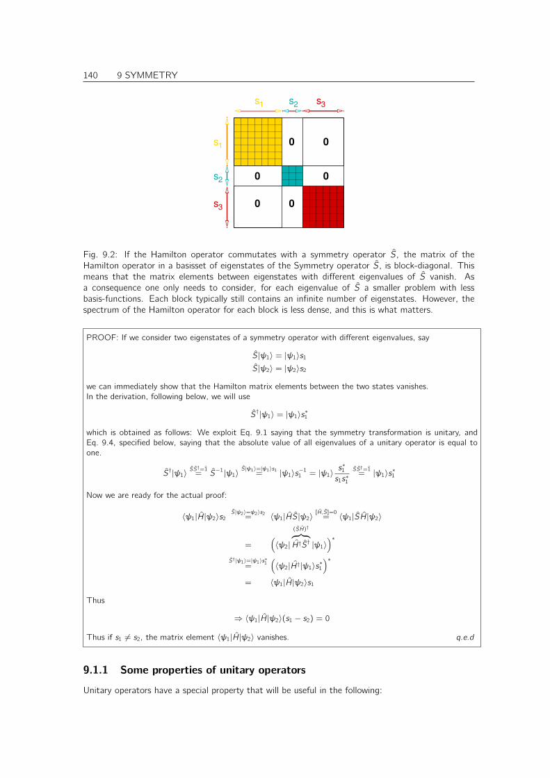
140 9 SYMMETRY
s
s1
s3
3
s
s
2
0 0
0
00
0
s21
Fig. 9.2: If the Hamilton operator commutates with a symmetry operator S, the matrix of theHamilton operator in a basisset of eigenstates of the Symmetry operator S, is block-diagonal. Thismeans that the matrix elements between eigenstates with different eigenvalues of S vanish. Asa consequence one only needs to consider, for each eigenvalue of S a smaller problem with lessbasis-functions. Each block typically still contains an infinite number of eigenstates. However, thespectrum of the Hamilton operator for each block is less dense, and this is what matters.
PROOF: If we consider two eigenstates of a symmetry operator with different eigenvalues, say
S|ψ1〉 = |ψ1〉s1
S|ψ2〉 = |ψ2〉s2
we can immediately show that the Hamilton matrix elements between the two states vanishes.In the derivation, following below, we will use
S†|ψ1〉 = |ψ1〉s∗1
which is obtained as follows: We exploit Eq. 9.1 saying that the symmetry transformation is unitary, andEq. 9.4, specified below, saying that the absolute value of all eigenvalues of a unitary operator is equal toone.
S†|ψ1〉SS†=1
= S−1|ψ1〉S|ψ1〉=|ψ1〉s1
= |ψ1〉s−11 = |ψ1〉
s∗1s1s∗1
SS†=1= |ψ1〉s∗1
Now we are ready for the actual proof:
〈ψ1|H|ψ2〉s2S|ψ2〉=ψ2〉s2
= 〈ψ1|HS|ψ2〉[H,S]=0
= 〈ψ1|SH|ψ2〉
=(〈ψ2|
(SH)†︷ ︸︸ ︷H†S† |ψ1〉
)∗S†|ψ1〉=|ψ1〉s∗1
=(〈ψ2|H†|ψ1〉s∗1
)∗= 〈ψ1|H|ψ2〉s1
Thus
⇒ 〈ψ1|H|ψ2〉(s1 − s2) = 0
Thus if s1 6= s2, the matrix element 〈ψ1|H|ψ2〉 vanishes. q.e.d
9.1.1 Some properties of unitary operators
Unitary operators have a special property that will be useful in the following:

9 SYMMETRY 141
The absolute value of all eigenvalues of a unitary operator is one.
SS† = 1 ∧ S|ψ〉 = |ψ〉s ⇒ |s| = 1 (9.4)
Hence we can write its eigenvalues in the form eiγ with a real phase-angle γ.
PROOF: We use 〈ψ|S†S|ψ〉 = 〈ψ|ψ〉 with an eigenstate |ψ〉 of S to an eigenvalue α, i.e. S|ψ〉 = |ψ〉α.We find α∗〈ψ|ψ〉α = 〈ψ|ψ〉 and therefore α∗α = 1. The most general form for α fulfilling this condition isα = eiγ with a real γ. q.e.d.
9.1.2 Symmetry groups
A group G is a set of elements Sn with a binary operation (we will refer to it as multiplication, eventhough it may be a generalization of a multiplication) such that
• the product of two elements of the group is again an element of the group, that is
∀Sn,Sm∈G SnSm ∈ G
• there is a unity element 1 in the group so that
∀Sn∈G Sn1 = 1Sn = Sn
• for each element Sn in the group there is an inverse S−1n so that
∀Sn∈G∃S−1n ∈G SnS
−1n = S−1
n Sn = 1
For example, the set of integers with the addition is a group. In this case the addition plays therole of the operation in the group definition. The addition by zero plays the role of the multiplicationby the unit element.
It is important to remember that the multiplication does not need to commutate. If the multipli-cation commutates, ∀SnSm∈GSnSm = SmSn, then the group is called Abelian, otherwise it is callednon-Abelian.
A group is called finite, if it has a finite number of elements.
9.2 Finite symmetry groups
First, we consider finite symmetry groups, because they are simple to handle. An example for a finitegroup is the mirror reflection.
The eigenvalues of a symmetry operator S of a finite symmetry group, that is Sn = 1 with somepositive integer n, are e i2πj/n where j is any integer number from 0 to n − 1.

142 9 SYMMETRY
PROOF: Let us consider a series of operators in the group (. . . , S−1, 1, S, S2, . . .) If the group is finite, thisseries must be cyclic, i.e. we can find a number n so that Sj+n = Sj for all j . n must be smaller than or equalto the number of elements in the group. Thus we find, by applying S−j , that Sn = 1.Let us consider an eigenstate |ψ〉 of S, so that
S|ψ〉 = |ψ〉eiφ
We have shown that the eigenvalues of a unitary operator can be written as eiφ. Then we can show that |ψ〉is an eigenstate of Sj with eigenvalue eiφj .
Sj |ψ〉 = |ψ〉eiφj
Since on the other hand Sn = 1 we find that eiφn = 1 and therefore φ = 2π/n. Thus the eigenvalues areei2πj/n. q.e.d.
One can construct eigenstates of the symmetry operator S from any state |φ〉 by
|ψk〉 =
n−1∑j=0
Sj |φ〉e−i2πjk/n (9.5)
Note however, that the result of the sum may vanish.
Here we showa that the state defined in Eq. 9.5 is an eigenstate of S with eigenvalue ei2πk/n, where the seriesSi is cyclic with period n.Proof: We multiply |ψk〉 from Eq. 9.5 with S
S
n−1∑j=0
Sj |φ〉e−i2πjk/n︸ ︷︷ ︸|ψk 〉
=(n−1∑j=0
Sj+1|φ〉e−i2π(j+1)k/n)
ei2πk/n =(n−1∑j=0
Sj |φ〉e−i2πjk/n)
︸ ︷︷ ︸|ψk 〉
ei2πk/n
In the last step, we shifted the indices j + 1 → j and exploited that the series (Si) is cyclic with period n.Thus we have shown that |ψk〉 as defined in Eq. 9.5 obeys the eigenvalue equation.
S|ψk〉 = |ψk〉ei2πk/n
q.e.d.
aOne can derive the result by inserting an Ansatz |ψk 〉 =∑n−1j=0 S
j |φ〉cj,k into the eigenvalue equation S|ψk 〉 =
|ψk 〉e−i2πjk/n which results in a recursive relation for the coefficients cj,k .
9.3 Continuous symmetries
9.3.1 Shift operator
Let us now consider an operator Q and its canonical momentum P . The canonical momentum hasbeen defined in Eq. 5.26 by
[P , Q]Eq. 5.26
=~i.
We define a shift operator
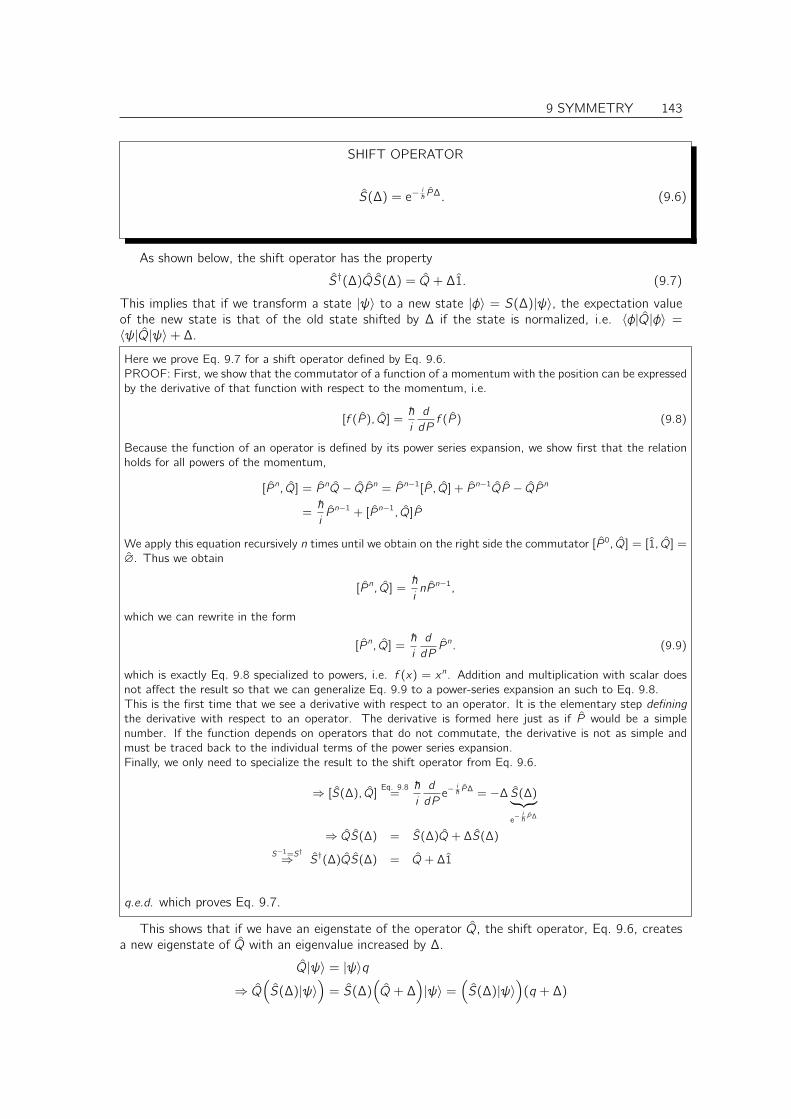
9 SYMMETRY 143
SHIFT OPERATOR
S(∆) = e−i~ P∆. (9.6)
As shown below, the shift operator has the property
S†(∆)QS(∆) = Q+ ∆1. (9.7)
This implies that if we transform a state |ψ〉 to a new state |φ〉 = S(∆)|ψ〉, the expectation valueof the new state is that of the old state shifted by ∆ if the state is normalized, i.e. 〈φ|Q|φ〉 =〈ψ|Q|ψ〉+ ∆.
Here we prove Eq. 9.7 for a shift operator defined by Eq. 9.6.PROOF: First, we show that the commutator of a function of a momentum with the position can be expressedby the derivative of that function with respect to the momentum, i.e.
[f (P ), Q] =~i
d
dPf (P ) (9.8)
Because the function of an operator is defined by its power series expansion, we show first that the relationholds for all powers of the momentum,
[P n, Q] = P nQ− QP n = P n−1[P , Q] + P n−1QP − QP n
=~iP n−1 + [P n−1, Q]P
We apply this equation recursively n times until we obtain on the right side the commutator [P 0, Q] = [1, Q] =
∅. Thus we obtain
[P n, Q] =~inP n−1,
which we can rewrite in the form
[P n, Q] =~i
d
dPP n. (9.9)
which is exactly Eq. 9.8 specialized to powers, i.e. f (x) = xn. Addition and multiplication with scalar doesnot affect the result so that we can generalize Eq. 9.9 to a power-series expansion an such to Eq. 9.8.This is the first time that we see a derivative with respect to an operator. It is the elementary step definingthe derivative with respect to an operator. The derivative is formed here just as if P would be a simplenumber. If the function depends on operators that do not commutate, the derivative is not as simple andmust be traced back to the individual terms of the power series expansion.Finally, we only need to specialize the result to the shift operator from Eq. 9.6.
⇒ [S(∆), Q]Eq. 9.8
=~i
d
dPe−
i~ P∆ = −∆ S(∆)︸ ︷︷ ︸
e− i~ P∆
⇒ QS(∆) = S(∆)Q+ ∆S(∆)
S−1=S†⇒ S†(∆)QS(∆) = Q+ ∆1
q.e.d. which proves Eq. 9.7.
This shows that if we have an eigenstate of the operator Q, the shift operator, Eq. 9.6, createsa new eigenstate of Q with an eigenvalue increased by ∆.
Q|ψ〉 = |ψ〉q
⇒ Q(S(∆)|ψ〉
)= S(∆)
(Q+ ∆
)|ψ〉 =
(S(∆)|ψ〉
)(q + ∆)

144 9 SYMMETRY
So far we have started from the canonical momentum P and constructed the shift operatorvia Eq. 9.6. Now we go the opposite direction and start out from the shift operator and derivethe canonical momentum from it. This will show the intricate relationship between momenta andsymmetry.
If the shift operator S for an operator Q obeying Eq. 9.7 is known, then we can construct thecanonical momentum using
S(∆) = e−i~ P∆ = 1−
i
~P∆ +O(∆2)
i~S(∆)− 1
∆= P +O(∆)
Thus we obtain an expression that allows us to obtain the canonical momentum to any variable,for which the corresponding shift operator is known.
CANONICAL MOMENTUM
P = i~ lim∆→0
S(∆)− 1
∆(9.10)
9.4 Recommended exercises
1. Construct the translation operator from the canonical momentum Exercise 16.4 on p. 236

Chapter 10
Specific Symmetries
10.1 Parity
An example of a finite group is the inversion:
S =
∫dx | − x〉〈x |
Sψ(x) = 〈x |S|ψ〉 = 〈x |∫dx ′| − x ′〉〈x ′|︸ ︷︷ ︸
S
|ψ〉 =
∫dx ′ 〈x | − x ′〉︸ ︷︷ ︸
δ(x+x ′)
〈x ′|ψ〉︸ ︷︷ ︸ψ(x ′)
=
∫dx ′δ(x + x ′)ψ(x ′) = ψ(−x)
The group has the elements (1, S)
Since S2 = 1 we find two eigenvalues s1 = 1 and s2 = −1. If the eigenvalue is +1 we say thestate has parity one or the state is even. If it is −1 we say the state has parity minus one or thatthe state is odd.
Example: We expect that a system is inversion symmetric, if the potential is inversion symmetric,such as the particle in the box. If we place the zero in the center of the box, then the inversion doesnot change the potential. As a consequence of the symmetry, the eigenstates shown in Fig. 4.4 onp. 60, are either symmetric or antisymmetric with respect to the inversion: The symmetric stateshave parity s = 1, while the antisymmetric states have parity s = −1.
In the following we show that the inversion symmetry can be traced back to the inversion symmetryof the potential. It seems obvious that an inversion symmetric potential leads to a inversion symmetricproblem. Nevertheless this nearly trivial exercise may be helpful to demonstrate the principle ofshowing the symmetry of a quantum mechanical problem.
H =
∫dx |x〉
(−~2
2m∂2x + v(x)
)〈x | = T + V
T =
∫dx |x〉
−~2
2m∂2x 〈x |
V =
∫dx |x〉v(x)〈x |
In order to verify that the system is symmetric with respect to inversion we need to show that
145

146 10 SPECIFIC SYMMETRIES
the Hamilton operator commutes with the inversion operator.
[T , S] =
∫dx |x〉
−~2
2m∂2x 〈x |︸ ︷︷ ︸
T
∫dx ′| − x ′〉〈x ′|︸ ︷︷ ︸
S
−∫dx ′ |x ′〉〈−x ′|︸ ︷︷ ︸
S
∫dx |x〉
−~2
2m∂2x 〈x |︸ ︷︷ ︸
T
=
∫dx |x〉
−~2
2m∂2x
∫dx ′ 〈x | − x ′〉︸ ︷︷ ︸
δx+x ′
〈x ′| −∫dx ′
∫dx |x ′〉 〈−x ′|x〉︸ ︷︷ ︸
δ(x+x ′)
−~2
2m∂2x 〈x |
=
∫dx |x〉
−~2
2m∂2x 〈−x | −
∫dx | − x〉
−~2
2m∂2x 〈x | = 0
In the last step we performed a variable transform x → −x on the right-hand part.1 2 Thus we haveshown that the kinetic energy commutates with the inversion operator.
Now we need to investigate the potential operator
[V , S] =
∫dx |x〉v(x)〈x |︸ ︷︷ ︸
V
∫dx ′| − x ′〉〈x ′|︸ ︷︷ ︸
S
−∫dx ′ |x ′〉〈−x ′|︸ ︷︷ ︸
S
∫dx |x〉v(x)〈x |︸ ︷︷ ︸
V
=
∫dx
∫dx ′|x〉v(x) 〈x | − x ′〉︸ ︷︷ ︸
δ(x+x ′)
〈x ′| −∫dx ′
∫dx |x ′〉 〈−x ′|x〉︸ ︷︷ ︸
δ(x+x ′)
v(x)〈x |
=
∫dx |x〉v(x)〈−x | −
∫dx ′|x ′〉v(−x ′)〈−x ′|
=
∫dx |x〉
(v(x)− v(−x)
)〈−x |
Thus the commutator [H, S] between the hamiltonian and the parity operator vanishes, if the potentialis itself inversion symmetric, i.e. v(x) = v(−x). Thus the Hamiltonian is symmetric under the parityoperation, if the parity operation transforms the potential on itself. Remember that this is not truefor the wave function: The wave functions of a parity symmetric system are either symmetric orantisymmetric under the parity operation.
10.2 n-fold rotation about an axis
Consider an n-fold rotation in space, which is described by a unitary matrix U
~r ′ = U~r
Since U describes a n-fold rotation, Un = 111.1Variable transform:
y(x) = −x ⇒ dy =dy
dxdx
y=−x= −dx∫ b
adxf (x) =
∫ y(b)
y(a)dy
(dy
dx
)f (x(y))
y=−x= −
∫ −b−a
dy f (−y) = +
∫ −a−b
dy f (−y)
∂2x = ∂x
(dy
dx∂y
)=d2y
dx2∂y +
(dy
dx
)2
∂2yy=−x
= ∂2y
2Here we show the identity for an arbitrary matrix element. which proves the operator identity.
〈φ|[T , S]|ψ〉 =
∫dx〈ψ|x〉
−~2
2m∂2x 〈−x |φ〉 −
∫dx 〈ψ| − x〉
−~2
2m∂2x 〈x |φ〉
=
∫dx ψ∗(x)
−~2
2m∂2xφ(−x)−
∫dx ψ∗(−x)
−~2
2m∂2xφ(x) = 0
10 SPECIFIC SYMMETRIES 147
The rotation in real space corresponds to a transformation S in Hilbert space.
S =
∫d3r |U~r〉〈~r |
Sψ(~r) = 〈~r |S|ψ〉 =
∫d3r ′ 〈~r |U~r ′〉︸ ︷︷ ︸
δ(~r−U~r ′)
〈~r ′|ψ〉︸ ︷︷ ︸ψ(~r ′)
det[U]=1;U−1=U†
= ψ(U†~r)
Note that the resolution of the delta function was non-trivial.3
Just as the rotation of real space point form a group with elements 111,U,U2, . . .Un−1 the groupof the corresponding symmetry operations in real space forms a group. The group has n elements,1, S, . . . , Sn−1. The eigenvalues of S are sj = ei2πj/n for j = 0, . . . , n − 1.
Editor: introduce here the example of ammonia, to show how eigenstates for a symmetryoperator are constructed
10.3 Exchange of two particles
If the exchange of two particles does not change the system, we call those particles identical. Thusthe presence of identical particles implies a symmetry. Unlike classical mechanics, this symmetry hasradical consequences in quantum mechanics.
The symmetry operation is the permutation P of two particles.
Pi ,j =
∫d3r1 · · ·
∫d3rN |~r1, . . . , ~rj , . . . , ~ri , . . . , ~rN〉〈~r1, . . . , ~ri , . . . , ~rj , . . . , ~rN |
The wave function that corresponds to the state |~r1, . . . , |~rN〉 is a product of δ-functions in the3N-dimensional configuration space centered at the positions ~r1, . . . , ~rN , i.e.
|ψ〉 = |~r1, . . . , ~rN〉 ⇒ ψ(~r ′1, . . . , ~r ′N) = 〈~r ′1, . . . , ~r ′N |~r1, . . . , ~rN〉 = δ(~r ′1 − ~r1) · · · δ(~r ′N − ~rN)
The permutation can be considered as a geometric operation in the 3N-dimensional configurationspace of all N particles. This is illustrated best by considering two one-dimensional particles as thesimplest possible case. The positions of the two particles are described by two coordinates (x1, x2).The permutation of the two particles corresponds to a mirror operation about the main diagonal ofthe x1 − x2-plane. This is illustrated in Fig. 10.3.1 on p. 150.
Let us now consider a wave function ψ(~r1, ~r2, . . . , ~rN) for many particles and the permutation oftwo particles as symmetry operator.
Pi ,jψ(. . . , ~ri , . . . , ~rj . . .) = ψ(. . . , ~rj , . . . , ~ri . . .)
For the interchange of every two particles we have a symmetry group with two elements and eigen-values 1 and −1.
For identical particles there exists no Hamilton operator that is not invariant with respect toparticle exchange. If there would be one, then it would be possible to devise and experiment thatdistinguishes between the particles. If we can distinguish between particles, they are obviously nomore be identical. Since this is not the case, each Hamilton operator commutates with the particleexchange of identical particles. Thus all particles are either symmetric or antisymmetric with respectto particle exchange. Accordingly, particles can be classified as being either Fermions or Bosons.
3In one dimension the identity δ(ax) = 1aδ(x) holds. In three dimension this translates into δ(A~x) = 1
detAδ(~x). In
the operation used in the text, the prefactor vanishes, because U is unitary and therefore detU = 1

148 10 SPECIFIC SYMMETRIES
FERMIONS AND BOSONS
Fermions Bosonswave function antisymmetric under permutation wave function symmetric under permutationhalf-integer spin integer spinPauli principle macroscopic quantum states possible
(e.g. Bose Einstein condensation, Laser)“particles” “interactions”
Examples: Exampleselectron photon (electrodynamics)proton graviton (gravity)neutron Z- and W-boson (weak force)quark gluon (strong force)
Higgs bosonphononexciton
10.3.1 Fermions
Particles that are antisymmetric under particle exchange are called Fermions. All Fermions have ahalf-integer spin. (The concept of spin will be introduced later.) Examples for Fermions are electrons,protons, quarks. An important consequence of the antisymmetry is the Pauli principle, which saysthat no two Fermions can occupy the same site or the same one-particle state.
Let us show that two identical Fermions cannot occupy the same site. The wave function ampli-tude for two particles at the same position ~r0 and all others on arbitrary positions is
ψ(. . . , ~r (0)︸︷︷︸pos.i
, . . . , ~r (0)︸︷︷︸pos.j
, . . .)
Exchanging the two particle coordinates, one obtains , on the one hand, the same result, on theother hand we obtain a sign change due to particle permutation. Thus:
ψ(. . . , ~r (0)︸︷︷︸pos.i
, . . . , ~r (0)︸︷︷︸pos.j
, . . .) = −ψ(. . . , ~r (0)︸︷︷︸pos.i
, . . . , ~r (0)︸︷︷︸pos.j
, . . .)
This is only possible if the wave function amplitude vanishes, whenever two particles have the sameposition.4 The probability that the two particles are at ~r0 is obtained from the absolute square of thewave function integrated over all particle positions except particles i and j . This probability vanishesas well.
PAULI PRINCIPLE
• The probability of finding two identical Fermions in the same position vanishes
• Two identical Fermions cannot occupy the same one-particle state.
Let us now consider a product state Ψ(~r1, ~r2) = φ1(~r1)φ2(~r2). Product states are the mostsimple many particle wave functions. They play an important role for non-interacting particles.
4If the two particles are at the same position the value of the wave function does not change under permutation.On the other hand the wave function has to change its sign. Thus the wave function vanishes for identical positions.

10 SPECIFIC SYMMETRIES 149
For non-interacting particles the N-particle Hamiltonian H(N) =∑N
i=1 H(1)i is a sum of one-particle
Hamiltonians, where the one-particle Hamiltonian H(1)i only acts on the coordinates of the i-th
particle. For non-interacting particles, we can use the method of separation of variables to expressthe eigenstates as a product of wave functions of the one-particle wave functions, that is a productstate. The energy is then the sum of the corresponding one-particle energies.
However, a product state does not have the symmetry or antisymmetry required for identicalparticles. Thus we need to antisymmetrize the wave function. We can anti-symmetrize this state anaccording to our recipe from Eq. 9.5. In the two-particle case we obtain
ΨF (~r1, ~r2) =1√2!
[φ1(~r1)φ2(~r2)− φ2(~r1)φ1(~r2)
]Here we can easily verify that the Pauli principle holds: the wave function vanishes if φ1(r) = φ2(r).Thus we have shown that one cannot place two identical Fermions into a single one-particle state.
An antisymmetric wave function can be written in a more general way as a Slater determinant
ΨF (~r1, . . . , ~rN) =1√N!
det
φ1(~r1) φ1(~r2) · · · φ1(~rN)
φ2(~r1) φ2(~r2) · · · φ2(~rN)...
......
...φN(~r1) φN(~r2) · · · φN(~rN)
From the property of that the determinant it changes its sign under exchange of two columns,we obtain antisymmetry. Not every antisymmetric wave function can be represented as a Slaterdeterminant. The most general form of a Fermionic wave function of N particles is a superpositionof all N-particle Slater determinants that can be formed from a complete set of one-particle states.
Not every N-particle state can be expressed as a single Slater determinant. However, if weform all possible the Slater determinants from the eigenstates of a one-particle Hamiltonian h, weobtain a complete basisset of the Hilbert space of Fermionic, i.e. antisymmetric, N-particle states.These Slater-determinants are the eigenstates of the non-interacting N-particle Hamiltonian H(N) =∑N
i=1 H(1)i . For identical particles, each one-particle Hamiltonian H(1)
i is identical to all others exceptthat it acts on the coordinates of a specified, namely the i-th, particle. The eigenstates of anobservable such as the N-particle Hamiltonian forms a complete basisset. A general N-particle wavefunction can thus be written as a Multiconfiguration wave function, namely as a sum of all Slaterdeterminants that can be built from a complete one-particle basisset.
The energy eigenstates of non-interacting Fermions can be expressed as single Slater determinantsmade from the eigenstates of the corresponding one-particle Hamiltonian. The wave functions ofinteracting particles must be written as multiconfiguration wave functions. Multiconfiguration wavefunctions are notoriously difficult to describe. However there are techniques such as density functionaltheory, that allow to map a system of interacting electrons onto a system of non-interacting particles.The latter allow us to effectively deal with wave functions that are single Slater determinants.
10.3.2 Bosons
Particles that are symmetric under particle exchange are called Bosons. All Bosons have an integerspin. (The concept of spin will be introduced later.) Examples for bosons are photons, mesons.Typically they are related to interactions such as the Coulomb interaction.
I can form a Bosonic state as a symmetrized product of a single one-particle states. For a twoparticle state built from two one-particle orbitals φ1(~r) and φ2(~r)one obtains
ΨB(~r1, ~r2) =1√2
(φ1(~r1)φ2(~r2) + φ2(~r1)φ1(~r2))
This can be generalized to many particles as follows:
ΨB(~r1, ~r2, . . . , ~rN) =∏i<j
1√2
(1 + Pi ,j)φ(~r1)φ(~r2) . . . φ(~rN)

150 10 SPECIFIC SYMMETRIES
x1
x2
Fig. 10.1: Wave function of two fermions in a one-dimensional box. One axis represents the positionof the first particle and the other axis that of the other. The problem of two particles in a one-dimensional box is analogous to that of one-particle in a two dimensional box. The symmetry withrespect to particle exchange corresponds to a mirror plane at the diagonal x1 = x2. The antisymmetryforces a node plane to lie at the diagonal x1 = x2. The lower figure shows a contour plot of the wavefunction. The different signs are indicated by the different colors. The functions on the right indicatethe wave function (dashed) and the density (filled line) of the first particle for a fixed position of thesecond. The position of the second is marked by the black ball.

10 SPECIFIC SYMMETRIES 151
where the operator Pi ,j permutes the coordinates ~ri and ~rj Thus we can place an macroscopic numberof Bosons into a single one-particle state. Such a state is called a macroscopic quantum state,and it allows quantum properties to be observed in the macroscopic . An example for such a state islaser light. Another example is the superfluid state of liquid Helium, which flows without dissipationand has infinite viscosity. Superconductivity is the result of conduction electrons forming pairs, whichare Bosons, and the condensation of these pairs into a single one-particle orbital. Even Atoms canbe prepared in a Bosonic state, which undergoes Bose-Einstein condensation and then all atoms areplaced in a macroscopic quantum state.
10.4 Continuous translations
The translation operator, which translates a state in x-direction, is defined by
S =
∫dx |x + ∆〉〈x |
S(∆)Ψ(x) = 〈x |S|ψ〉 =
∫dx ′ 〈x |x ′ + ∆〉︸ ︷︷ ︸
δ(x ′+∆−x)
〈x ′|ψ〉 = 〈x − ∆|ψ〉 = Ψ(x − ∆)
Note here the minus sign in the argument: If S(∆) shifts the wave function to the right, the valuesfor the new wave function are obtained from the unshifted wave function at a position to the left.
We obtain the conjugate momentum by
pxEq. 9.10
= i~ lim∆→0
1
∆
∫dx(|x + ∆〉〈x | − |x〉〈x |
)= i~ lim
∆→0
1
∆
∫dx(|x〉〈x − ∆| − |x〉〈x |
)= i~
∫dx |x〉 lim
∆→0
〈x − ∆| − 〈x |∆︸ ︷︷ ︸
−∂x 〈x |
=
∫dx |x〉
~i∂x 〈x |
pxΨ(x) = 〈x |px |ψ〉 =
∫dx ′ 〈x |x ′〉︸ ︷︷ ︸
δ(x−x ′)
~i∂x ′ 〈x ′|ψ〉︸ ︷︷ ︸
ψ(x ′)
=~i∂xψ(x)
Thus we have derived the explicit form for the momentum operator from the shift operator.The generalization to a translation in three dimensions is straightforward:
S(~∆) =
∫d3r |~r + ~∆〉〈~r |
S(~∆)Ψ(~r) = Ψ(~r − ~∆)
~p =
∫d3r |~r〉
~i~∇〈~r |
The eigenstates |ψ~k〉 of the shift operator can be obtained from the eigenvalue equation of themomentum operator
pψ~k(~r) = ψ~k(~r)~~k ⇒ S(~∆)Ψ~k(~r) = Ψ~k(~r − ~∆)Eq. 9.6
= Ψ~k(~r)e−i~k~∆ (10.1)

152 10 SPECIFIC SYMMETRIES
where ~~k are here the eigenvalues of the momentum operator. By setting ~r = ~0 and replacing ~∆ by−~r in Eq. 10.1, we find that the eigenstates of the translation operator, which are also momentumeigenstates have the from of plane waves.
Ψ~k(~r − ~∆)Eq. 10.1
= Ψ~k(~r)e−i~k~∆
~r→~0; ~∆→−~r⇒ Ψ~k(~0− (−~r)) = Ψ~k(~0)e−i~k(−~r)
⇒ Ψ~k(~r) = Ψ~k(~0)ei~k~r (10.2)
EIGENSTATES OF THE TRANSLATION OPERATOR
The eigenstates of the translation operator,
S(~∆)|ψ~k〉 = |ψ~k〉e−i~k~∆ (10.3)
are plane waves
Ψ~k(~r)Eq. 10.2
= A ei~k~r (10.4)
The eigenstates of the shift operator are also the eigenstates of the corresponding momentum oper-ator, i.e.
p|ψ~k〉 = |ψ~k〉~~k
This is the reason for using plane waves as Ansatz, when we search a solution for a differentialequation with translational symmetry. Because the result rests on symmetry, this Ansatz is verygeneral and works for any kind of differential equation.
10.5 Discrete translations, crystals and Bloch theorem
Most solids are crystals. This implies that the atoms are located on regular positions. The clearestevidence of this regular arrangement are the crystal faces of gem stones. This arrangement results ina symmetry, the lattice periodicity. Lattice translation symmetry is a discrete translational symmetry.
10.5.1 Real and reciprocal lattice: One-dimensional example
Let us consider a linear chain of hydrogen atoms as the most simple model of a one-dimensionallyperiodic crystal of hydrogen atoms shown in Fig. 10.2. It is a model system, which is not stable inreality. However it allows to develop the concepts.

10 SPECIFIC SYMMETRIES 153
T a
Fig. 10.2: Linear chain of hydrogen atoms. The lattice spacing is a. The balls represent the atoms.The graph sketched below represents the potential as function of position. The primitive latticevector is ~T which has the length a. The primitive reciprocal lattice vector has the length 2π/a.
The periodicity of the chain implies that for every atom at position ~R0 there are also equivalentatoms at the positions ~Rn = ~R0 + n~T , where n is any integer. ~T is the primitive lattice vector.General lattice vectors are ~tn = n~T . The primitive lattice vector is the smallest possible latticevector, that fully describes the lattice periodicity. Its length is called the lattice constant a.
Not only the atomic positions are regular, but also the potential is periodic, that is v(~r + ~tn) =v(~r). A periodic potential has a discrete Fourier transform
v(~r) =∑n
ei~Gn~rVn
where the vectors ~Gn = n~g are the general reciprocal lattice vectors. The primitive reciprocallattice vector is denoted by ~g. The length of the primitive reciprocal lattice vector is inverselyproportional to the real-space lattice constant a, that is |~g| = 2π
a
10.5.2 Real and reciprocal lattice in three dimensions
Let us now generalize the expressions to three a three-dimensional lattice. Fig. 10.5.2 demonstratesthe concepts developed in the following. Corresponding to the three spatial directions there are nowthree primitive lattice vectors, which we denote by ~T1, ~T2, ~T3. Note that in two or three dimensionsthere is no unique choice of primitive lattice vectors. The three primitive lattice vectors span theprimitive unit cell.
A general lattice vector ~ti ,j,k can be expressed by the primitive lattice vectors ~T1, ~T2, ~T3 as
~ti ,j,k = i ~T1 + j ~T2 + k ~T3=
Tx,1 Tx,2 Tx,3Ty,1 Ty,2 Ty,3
Tz,1 Tz,2 Tz,3
︸ ︷︷ ︸
T
i
j
k
where i , j, k are arbitrary integers.It is often convenient to combine the lattice vectors into a 3×3 matrix T as shown above. Often
the atomic positions ~Rn are provided in relative positions ~X which are defined as
~Rn = T ~Xn ⇔ ~Xn = T−1 ~Rn
A potential is called periodic with respect to these lattice translations, if V (~r + ~ti ,j,k) = V (~r).

154 10 SPECIFIC SYMMETRIES
RECIPROCAL LATTICE
The reciprocal lattice is given by those values of the wave vector ~G, for which the correspondingplane waves ei
~G~r have the same periodicity as the real-space lattice.The primitive reciprocal-lattice vectors ~gn for n = 1, 2, 3 are defined in three dimensions as
~gn~Tm = 2πδn,m (10.5)
Thus, in three dimensions the reciprocal lattice vectors can be obtained as
~g1 = 2π~T2 × ~T3
~T1
(~T2 × ~T3
) , ~g2 = 2π~T3 × ~T1
~T1
(~T2 × ~T3
) , ~g3 = 2π~T1 × ~T2
~T1
(~T2 × ~T3
)It is easily shown that these expressions fulfill the defining equation Eq. 10.5 for the reciprocal latticevectors. Note that the expressions for the second and third lattice vector are obtained from the firstby cyclic commutation of the indices.
Because the vector product is perpendicular to the two vectors forming it, every reciprocal latticevector is perpendicular to two real-space lattice vectors. This brings us to the physical meaning ofthe reciprocal lattice vectors: Two real space lattice vectors define a lattice plane. A plane can bedefined either by two linearly independent vectors in the plane or alternatively by the plane normal.The reciprocal lattice vectors apparently define lattice planes, because they are plane normals.
Let us now consider the distance ∆n of two neighboring lattice planes. It is obtained by projectingone vector pointing ~Tn from one plane to the other onto a normalized plane normal ~gn/|~gn|.
∆n = ~Tn~gn|~gn|
Eq. 10.5=
2π
|~gn|
⇒ |~gn| =2π
∆n
PHYSICAL MEANING OF RECIPROCAL LATTICE VECTORS
• The reciprocal lattice vectors are perpendicular to the lattice planes of the real-space lattice.
• The length of the primitive reciprocal lattice vectors is 2π divided by the distance of the latticeplanes.
We can form a 3× 3 matrix g from the three primitive reciprocal lattice vectors.
gdef=
gx,1 gx,2 gx,3gy,1 gy,2 gy,3
gz,1 gz,2 gz,3
The definition Eq. 10.5 of the reciprocal lattice vectors can be expressed in matrix form as
g>TEq. 10.5
= 2π111 (10.6)
Thus the matrix g is obtained as
gEq. 10.6
= 2π(T−1
)>(10.7)

10 SPECIFIC SYMMETRIES 155
The general reciprocal lattice vectors are
~Gi ,j,k = i~g1 + j~g2 + k~g3
The reciprocal lattice vectors play an important role in the Fourier transform of periodic functions.All plane waves that are periodic with the lattice vectors ~Tn are characterized by a reciprocal latticevector.
ei~G(~r+~Tn) = ei
~G~r
⇒ ~G(~r + ~Tn) = ~G~r + 2πmn
⇒ ~G~Tn = 2πmn
⇒ ~GT = 2π ~m
⇒ ~G = 2π ~mT−1 = 2π(T−1
)>~m
where mn are integers. The allowed values for ~G are exactly those of the reciprocal lattice. This wasthe motivation for the definition Eq. 10.6.

156 10 SPECIFIC SYMMETRIES
C6C3
∆ 2
∆ 1
t3,−2,0
T2
T1
g1
g2
Fig. 10.3: Translational and rotational symmetry of a single graphite sheet and demonstration ofreciprocal lattice vectors. Graphite is a layered material, which consists of sheets as the one shown.The yellow balls indicate the carbon atoms and the blue sticks represent the bonds. In graphite thesetwo-dimensional sheets are stacked on top of each other, where every second sheet is shifted suchthat an atom falls vertically below the point indicated by C6. Here we only consider the symmetryof a single sheet. The elementary unit cell is indicated by the red parallelogram, which is spanned bythe elementary lattice vectors ~T1 and ~T2. The third lattice vector points perpendicular to the sheettowards you. An example for a general lattice vector is ~t3,−2,0 = 3~T1− 2~T2 + 0~T3. The lattice planesindicated by the dashed lines. The lattice planes are perpendicular to the sheet. The distance of thelattice planes are indicated by ∆1 and ∆2. The elementary reciprocal lattice vectors are ~g1 and ~g2.The third reciprocal lattice vector points perpendicular out of the plane towards you. Note that thereciprocal lattice vectors have the unit “inverse length”. Thus their length is considered irrelevant inthis real space figure. The axis through C3 standing perpendicular to the plane is a three-fold rotationaxis of the graphite crystal. The axis through C6 perpendicular to the plane is a 6-fold rotation axis ofthe graphite sheet, but only a three-fold rotation axis of the graphite crystal. (Note that a rotationaxis for the graphite crystal must be one for both sheets of the crystal). In addition there is a mirrorplane lying in the plane. Furthermore there are several mirror planes perpendicular to the plane: Onepassing through every atom with one of the three bonds lying in the plane and one perpendiculareach bond passing through the bond center.

10 SPECIFIC SYMMETRIES 157
10.5.3 Bloch Theorem
BLOCH THEOREM:
The eigenstates of a system with lattice symmetry can be written as product of a periodic functionuk(~r) and a modulating plane wave ei
~k~r , that is
Ψk(~r)def= uk(~r)ei
~k~r (10.8)
where the Bloch vector ~k is a good quantum number of the system.More precisely: Lattice translation symmetry implies that there are lattice translation vectors~T1, ~T2, ~T3, so that the potential obeys V (~r + ~Ti) = V (~r). In that case the periodic function obeysu~k(~r + ~Ti) = u~k(~r), and the Bloch vectors ~k lie in one reciprocal unit cell.
PROOF: Because the system has lattice symmetry, the Hamilton operator commutates with the latticetranslation operator(Eq. 9.2). As a consequence we can form common eigenstates of the lattice translationoperator and the Hamilton operator. Thus the Hamilton operator is block diagonal in the basis of eigenstatesof the translation operator (Eq. 9.3). The eigenstates of the Hamilton operator can then be obtained bydiagonalizing the Hamilton operator in the subspace of all eigenvalues of the translation operator with agiven eigenvalue of the lattice translation vector. This is to be repeated for every eigenvalue of the latticetranslation operator. All this follows directly from what we have derived already.Now we need to find the eigenstates and eigenvalues for the lattice translation vector. The lattice translationoperator is defined by
S~Tn =
∫d3r |~r + ~Tn〉〈~r |
where ~Tn for n = 1, 2, 3 are the three primitive lattice translation vectors in real space. The result on a wavefunction is
S~TnΨ(~r)def= 〈~r |S~Tn |Ψ〉 = Ψ(~r − ~Tn)
We need not consider general translations, because the lattice translation operator for a general translationvector ~ti ,j,k = i ~T1 + j ~T2 + k ~T3 is the product of the those for the primitive lattice translation vectors.
S~ti ,j,k = Si~T1Sj~T2
Sk~T3
The lattice translation operator used for the lattice symmetry is the same as the continuous lattice translationvector, specialized to the lattice translations. The eigenvalues for the general lattice translation vector arealready known. The eigenvalue equation is
ψ(~r − ~Tn) = S~Tnψ(~r)Eq. 10.3
= ψ(~r)e−i~k ~Tn
·e−i~k(~r−~Tn)
⇒ ψ(~r − ~Tn)e−ik(~r−~Tn) = ψ(~r)e−i~k~r
Thus the function
uk(~r)def= ψ(~r)e−i
~k~r (10.9)
is periodic, that is
uk(~r − ~Tn) = uk(~r)
This is already what had to be proven: The eigenstates of the lattice translation operator for a given eigenvaluee−i
~k ~Tn , and thus the eigenstates of the Hamilton operator, have the form of a product of a periodic functionuk(~r) and modulated by a plane wave ei
~k~r . The wave function has the form
Ψk(~r)Eq. 10.9
= uk(~r)ei~k~r
q.e.d

158 10 SPECIFIC SYMMETRIES
We can define a k-dependent Hamiltonian for the periodic part u~k(~r) of the Bloch waves.
Hei~k~ru~k(~r) = ei
~k~ru~k(~r)En,~k
[e−i~k~r Hei
~k~r ]u~k(~r) = u~k(~r)En,~k
ˆH(~k) = e−i~k~r Hei
~k~r = e−i~k~r [
~p2
2m+ V (~r)]ei
~k~r =(~p + ~~k)2
2m+ V (~r)
=−~2
2m(~∇+ i~k)2 + V (~r)
The energies En(~k) are called band structure. They are the dispersion relations of the particles in aperiodic potential. Band structures exist for electrons, phonons and photons.
Fig. 10.4: Schematics of a calculated band structure of crystalline silicon [33].
The band structure is periodic in k-space. We show this as follows: We begin with some Blochwave Ψ~k,n(~r), which shall be also an eigenstate of the Hamiltonian with energy En(~k). We multiply
the periodic function u~k,n(~r) with e−i~G~r , which is itself periodic, and compensate by multiplication of
the phase factor with ei~G~r .
Ψ~k,n(~r) = u~k,n(~r)ei~k~r = [u~k,n(~r)e−i
~G~r ]ei(~k+~G)~r
Thus we have written the very same state as a Bloch wave
ψ~k+~G,n(~r) = u~k+~G,nei(~k+~G)~r
for the k-point ~k + ~G, with a periodic part
u~k+~G,n(~r)def= u~k(r)e−i
~G~r
and a phase ei(~k+~G)~r .
Because both function are identical, i.e. Ψ~k,n(~r) = Ψ~k+~G,n(~r), also the energies are the same.This shows that the band structure En(~k) is periodic in reciprocal space, i.e
En(~k) = En(~k + ~G)

10 SPECIFIC SYMMETRIES 159
10.5.4 Schrödinger equation in momentum representation
Editor: Construction! We can use the periodicity of the band structure to simplify its graphicalrepresentation. Let us consider a free particle. Clearly a completely translationally symmetric systemalso has lattice symmetry. The dispersion relation of a free particle is a parabola.
The wave functions of the free particle have the form
φ~G(~r) = ei~G~r = 〈~r |~G〉
and the eigenvalues are
E~G =(~~G)2
2m
Now we can consider the Hamiltonian in plane waves. A general state can be expressed in its Fourierrepresentation |~G〉 as
|Ψ〉 =
∫d3G
(2π)3|~G〉c(~G)
∫d3G′
(2π)3〈~G|H − E|~G′〉c(~G) = 0∫
d3G′
(2π)3〈~G|∫d3r |~r〉
(−~2
2m~∇2 + V (~r)− E
)〈~r |︸ ︷︷ ︸
H
|~G′〉c(~G) = 0
∫d3G′
(2π)3
∫d3r 〈~G|~r〉︸ ︷︷ ︸
e−i ~G~r
(−~2
2m~∇2 + V (~r)− E
)〈~r |~G′〉︸ ︷︷ ︸
ei~G′~r
c(~G) = 0
∫d3G′
(2π)3
∫d3r e−i
~G~r
(−~2
2m~∇2 + V (~r)− E
)ei~G′~rc(~G) = 0∫
d3G′
(2π)3
∫d3r
(~2 ~G′
2
2m+ V (~r)− E
)ei(
~G′−~G)~rc(~G) = 0
∫d3G′
(2π)3
(~2 ~G′
2
2m(2π)3δ(~G − ~G′) + V (~G − ~G′)− E(2π)3δ(~G − ~G′)
)c(~G) = 0
V (~G) =
∫d3r V (~r)ei
~G~r
Thus we obtain the form(~2 ~G′
2
2m− E
)c(~G) +
∫d3G′
(2π)3V (~G − ~G′)c(~G′) = 0
We can describe this in the form that the potential transfers a momentum ~(~G− ~G′) to an electron.If the potential is periodic its Fourier transform isEditor: Check
V (~G) =∑i ,j,k
(2π)3V (~Gi ,j,k)δ(~G − ~Gi ,j,k)
Thus we obtain the form(~2 ~G′
2
2m− E
)c(~G) +
∑i ,j,k
V (~Gi ,j,k)c(~G + ~Gi ,j,k) = 0

160 10 SPECIFIC SYMMETRIES
If we make the Ansatz c(~G) = c~k,i,j,kδ(~G −
(~k +
∑i ,j,k
~Gi ,j,k
))we immediately observe that the
Schrödinger equation can be solved independently for each set of coefficients with different ~k .Thus it makes sense to draw the energies of the basis states for each ~k on top of each other.
Thus we obtain the reduced zone scheme. If we again fold out the states, we obtain the extendedzone scheme.
We will see later in the chapter on first order perturbation theory, that the energies that lie closeto each other “repel” each other. This repulsion is strongest if the energy spacing is small. This leadsto an opening of the band gap wherever two bands in the reduced zone scheme meet.
2π
a
E
k
Fig. 10.5: If a free particle experiences a potential with periodicity a, states with wave vectors thatdiffer by a reciprocal lattice vector Gn = 2π
a n couple. The coupling shifts the upper state up andthe lower state down, which results in an opening of the gap. As a result of the coupling, the wavevector of a free particle state is no more a good quantum number. However, the wave vector in thereduced zone scheme remains to be a good quantum number.
10.6 Some common Lattices
10.6.1 Cubic lattices
aa
a
aa
a
aa
a
Fig. 10.6: The simple-cubic, the face-centered cubic and the body-centered cubic lattice in the simplecubic unit cell.
The most simple lattice is the simple cubic (sic) lattice which has lattice vectors
~T1 =
1
0
0
a , ~T2 =
0
1
0
a , ~T3 =
0
0
1
a

10 SPECIFIC SYMMETRIES 161
where a is the lattice constant. I am not aware of any crystal with one atom per unit cell that isstable in the simple cubic lattice.
More common is the face-centered cubic (fcc) lattice with lattice vectors
~T1 =
01212
a , ~T2 =
12
012
a , ~T3 =
1212
0
aThe face centered cubic lattice corresponds to one of the possible lattices of closed packed spheres.It is very common for atoms which do not form directed bonds. One example are noble gases, whenthey freeze. Another are metals such as Sodium, Aluminium, Gold, Copper, Silver. Austenite, themajor component of Steel is another example for a fcc-crystal.
The third cubic lattice is the body-centered cubic (bcc) lattice with lattice vectors
~T1 =
− 12
1212
a , ~T2 =
12
− 12
12
a , ~T3 =
1212
− 12
aThe body centered cubic lattice is found for metals, that form some extend of directed bonds, suchas the transition metals in the middle of the transition metal row. One example is iron in its magneticform
10.7 Recommended exercises
1. Symmetrization of states with a discrete symmetry: Exercise 16.6 on p. 238 (No workedsolutions)
2. Kronig-Penney model: Exercise 16.7 on p. 239 is an application of the Bloch theorem.

162 10 SPECIFIC SYMMETRIES

Chapter 11
Rotations, Angular Momentum andSpin
Systems with rotational symmetry play such an important role, that we devote a separate chapter tothem, even though what is done here is only an extension of what we learned in the section aboutsymmetry.
11.1 Rotations
Let us consider first a continuous rotation about the z-axis. The symmetry operator transforms ~rinto ~r ′ = R(ϕ)~r , where R(ϕ) is the corresponding rotation matrix.
(x ′
y ′
)=
(cos(ϕ) − sin(ϕ)
sin(ϕ) cos(ϕ)
)︸ ︷︷ ︸
R
(x
y
)
The angle is positive for counterclockwise rotation.A rotation of a wave function by an angle ϕ is then defined as
S(ϕ)def=
∫d3r |R(ϕ)~r〉〈~r | (11.1)
〈~r |S(ϕ)|ψ〉︸ ︷︷ ︸S(ϕ)ψ(~r)
=
∫d3r 〈~r |R~r〉〈~r |ψ〉 =
∫d3r 〈R−1~r |~r〉〈~r |ψ〉 = 〈R−1~r |ψ〉︸ ︷︷ ︸
ψ(R−1~r)
Note, that we need to use the inverse rotation, because we obtain the value of the rotated wavefunction at a point r0 by looking up the value of the original wave function at the position whichfell into r0 by the rotation. The inverse of the rotation is simply its transpose, because the rotationmatrix is unitary.
163

164 11 ROTATIONS, ANGULAR MOMENTUM AND SPIN
11.1.1 Derivation of the Angular momentum
Let us construct the canonical conjugate momentum L to the angle ϕ. We will see that L is theangular momentum.
Lzψ(x, y) = i~ limϕ→0
( S(ϕ)− 1
ϕ
)ψ(x, y)
= i~ limϕ→0
(ψ[
1+O(ϕ2)︷ ︸︸ ︷cos(ϕ) x +
ϕ+O(ϕ2)︷ ︸︸ ︷sin(ϕ) y ,−
ϕ+O(ϕ2)︷ ︸︸ ︷sin(ϕ) x +
1+O(ϕ2)︷ ︸︸ ︷cos(ϕ) y ]− ψ[x, y ]
ϕ
)
= i~ limϕ→0
(ψ(x,y)+(x+ϕy+O(ϕ)2)∂xψ+(y−ϕx+O(ϕ)2)∂yψ+...︷ ︸︸ ︷ψ[x + ϕy +O(ϕ2), y − ϕx +O(ϕ2)] −ψ[x, y ]
ϕ
)= i~ lim
ϕ→0
(ϕy∂xψ − ϕx∂yψ +O(ϕ2)
ϕ
)=~i
(−y∂x + x∂y
)ψ
Lz = x py − y px
Thus we obtained the form of the expression of the angular-momentum operator.Editor: Use the above example as exercise for a Taylor expansionWe can generalize this result into three dimensions for a rotation about an axis, which is described
by a vector ~ϕ. The direction of the vector describes the rotation axis and the length of the vectordenotes the angle of rotation.
Definition 11.1 ANGULAR-MOMENTUM OPERATORThe angular-momentum operator ~L has the form.
~L = ~r × ~p (11.2)
With the angular-momentum operator we can express the rotation operator S(ϕ) as
ROTATION OPERATOR
S(ϕ)Eq. 11.1
=
∫d3r |R~r〉〈~r | Eq. 9.6
= e−i~ Lxϕ (11.3)
11.1.2 Another derivation of the angular momentum (Home study)
This derivation is more complex but may also show some aspects more clearly. It does not referto wave functions and rests entirely within Dirac’s bracket notation. In any case it is a very goodexercise for the latter.
Lz = i~ limϕ→0
1
ϕ
[S(ϕ)− 1
]= i~ lim
ϕ→0
1
ϕ
[∫d3r |R(ϕ)~r〉〈~r | −
∫d3r |~r〉〈~r |
]= i~
∫d3r lim
ϕ→0
1
ϕ[|R(ϕ)~r〉 − |~r〉] 〈~r

11 ROTATIONS, ANGULAR MOMENTUM AND SPIN 165
Next we Taylor-expand the rotated vector R(ϕ)~r up to first order in ϕ.
R(ϕ) =
cos(ϕ) − sin(ϕ) 0
sin(ϕ) cos(ϕ) 0
0 0 1
=
1 +O(ϕ2) −ϕ+O(ϕ2) 0
ϕ+O(ϕ2) 1 +O(ϕ2) 0
0 0 1
= 111 +
0 −1 0
1 0 0
0 0 0
ϕ+O(ϕ2)
⇒ R~r = ~r +
−yx0
ϕ+O(ϕ2) = ~r + ϕ~ez × ~r +O(ϕ)2
Let us now use the translation operator T (~∆)def=∫d3r |~r + ~∆〉〈~r | to express the rotated state
|R(ϕ)~r〉 = |~r + ϕ~ez × ~r +O(ϕ2)︸ ︷︷ ︸∆
〉 = T (ϕ~ez × ~r +O(ϕ2)︸ ︷︷ ︸∆
)|~r〉
Eq. 9.6= e−
i~ ~p
∆︷ ︸︸ ︷(ϕ~ez × ~r +O(ϕ2)
)︸ ︷︷ ︸T (∆)
|~r〉
Tay lor=
[1−
i
~~pϕ(~ez × ~r) +O(ϕ2)
]|~r〉
~a(~b×~c)=~b(~c×~a)=
[1−
i
~~ez(~r × ~p)ϕ+O(ϕ2)
]|~r〉
Thus we obtain
Lz = i~∫d3r lim
ϕ→0
(−i
~~ez(~r × ~p)ϕ+O(ϕ2)
)︸ ︷︷ ︸
1i~ ~ez (~r×~p)
|~r〉〈~r | = ~ez(
∫d3r |~r〉~r〈~r |︸ ︷︷ ︸
~r
×~p)
= ~ez(~r × ~p)
Since we can choose our coordinate system arbitrarily we can immediately generalize the result directlyto arbitrary directions of the rotation axis, which identifies the angular-momentum operator as
~L = ~r × ~p
11.2 Commutator Relations
It turns out that the components of the angular momentum operator do not commutate with eachother. Therefore, it is not possible to determine the direction of the angular momentum with certainty.Let us now explore the commutator relations among the angular momentum operators.
[Lx , Ly ] = [y pz − z py , z px − x pz ]
= y pz z px − y pz x pz − z py z px + z py x pz
− z px y pz + z px z py + x pz y pz − x pz z py= y px [pz , z ] + py x [z , pz ] = i~(x py − y px)
= i~Lz

166 11 ROTATIONS, ANGULAR MOMENTUM AND SPIN
The other commutators are obtained by cyclic permutation of indices.
[Lx , Ly ] = i~Lz ; [Ly , Lz ] = i~Lx ; [Lz , Lx ] = i~Ly
Furthermore we can show that ~L2 commutates with all components
[~L2, Lx ] = [L2x , Lx ]︸ ︷︷ ︸=0
+[L2y , Lx ] + [L2
z , Lx ]
=(L2y Lx
=0︷ ︸︸ ︷−Ly Lx Ly
)+(Ly Lx Ly −Lx L2
y
)+(L2z Lx
=0︷ ︸︸ ︷−Lz Lx Lz
)+(Lz Lx Lz −Lx L2
z
)= Ly [Ly , Lx ] + [Ly , Lx ]Ly + Lz [Lz , Lx ] + [Lz , Lx ]Lz
= i~(−Ly Lz − Lz Ly + Lz Ly + Ly Lz
)= 0
Cyclic permutation of indices yields the commutator relations with the remaining angular momentumcomponents. Thus we can measure the amplitude of the angular momentum and one component ofthe angular momentum simultaneously.
[Li , Lx ] [Li , Ly ] [Li , Lz ] [Li , ~L2]
[Lx , Li ] 0 i~Lz −i~Ly 0
[Ly , Li ] −i~Lz 0 i~Lx 0
[Lz , Li ] i~Ly −i~Lx 0 0
In short, we can write the result using the Levi-Civita Symbol1 as
COMMUTATOR RELATION OF ANGULAR MOMENTA
[Li , Lj ] = i~∑k
εi ,j,k Lk (11.4)
11.3 Algebraic derivation of the eigenvalue spectrum
In the following we will show the algebraic description of angular momentum, which will provide uswith the eigenvalues of angular momenta. The algebraic description is important, because we willfind eigenstates, that cannot be represented by a single-valued wave function. Any Ansatz of a realspace wave function will therefore fail to produce those eigenstates.
Shift operators revisited
We already made contact with shift operators in connection with continuous translations. There,it was possible use a shift operator to create new eigenstates from an existing eigenstate with ashifted eigenvalue. Here we use shift operators, that are not unitary operators and therefore are nosymmetry transformations. However, we can still use them to create new eigenstates of an operator.The concept of shift operators to create new eigenstates is analogous to that of the creation and
1The Levi-Civita symbol is the fully antisymmetric tensor defined as being equal to one if the indices are ascendingε1,2,3 = ε2,3,1 = ε3,1,2 = 1 am being −1 if the indices are descending, that is ε3,2,1 = ε1,3,2 = ε2,1,3 = −11. Iftwo indices are equal the Levi-Civita symbol vanishes. The Levi-Civita Symbol is used to describe the cross-product(~a × ~b)i =
∑j,k εi ,j,kajbk .
11 ROTATIONS, ANGULAR MOMENTUM AND SPIN 167
annihilation operators, that have been used in the algebraic treatment of the harmonic oscillator andthe two state system.
A shift operator A has a commutator with the shifted operator B, which is proportional to theshift operator itself. As a result, the shift operator produces a new eigenstate A|ψb〉 of B from anexisting one, |ψb〉 with a shifted eigenvalue, that is
[A, B] = cA and B|ψb〉 = |ψb〉b ⇒ B(A|ψb〉
)=(A|ψb〉
)(b − c)
We can confirm this easily:
BA|ψb〉 = A B|ψb〉︸ ︷︷ ︸|ψb〉b
−cA|ψ〉
B(A|ψb〉
)=(A|ψb〉
)(b − c)
Furthermore we can show that [A†, B] = −cA† if B is hermitian and c is a real number.
[A†, B] = A†B − BA† =(B†A− AB†
)† B=B†= −[A, B]†
c=c∗= −cA†
Hence we can use A† to create an eigenstate of B with eigenvalue b + c
B(A†|Ψ〉
)=(A†|Ψ〉
)(b + c)
Thus we can produce a whole series of eigenstates of B with equi-spaced eigenvalues, if we canonly find an operator with the property [A, B] = cA, where c is real. The series of eigenvalues isbound from below and above if there is a solution to A|ψ0〉 = 0 and to A†(n+1)|ψ0〉 = 0.
Shift operators for Lz
Such a shift operator A is a handy thing to have. Let us look for one that may be useful for angularmomentum operators. We consider
[Ly , Lz ] = i~Lx[Lz , Lx ] = i~Ly
which suggests that an operator L− = aLx + bLy may do the job. If we use this as Ansatz for[L−, Lz ] = cL−, we find one solution2 with a = 1, b = −i and C = ~.
Thus we define the shift operators
L− = Lx − i Ly (11.5)
L+ = Lx + i Ly = L†− (11.6)
They obey the commutation relations
[L−, Lz ] = ~L−; [L+, Lz ] = −~L+; [L−, ~L2] = 0; [L+, ~L
2] = 0
2 We use the ansatz L− = aLx + bLy and require
[L−, Lz ] = CL−
⇒ [aLx + bLy , Lz ]− = a[Lx , Lz ]− + b[Ly , Lz ]− = −i~aLy + i~bLx =(ib~Lx − ia~Ly
) != C
(aLx + bLy
)we obtain two conditions, namely aC = ib~ and bC = −ia~. Thus C = i~ b
a= −i~ a
b, which requires b2 = −a2 and
therefore b = ±ia. If we choose a = 1 and b = −ia, then C = ~. The other solution leads to L+ with an arbitraryscale factor.

168 11 ROTATIONS, ANGULAR MOMENTUM AND SPIN
The first two equations identify the operators L+ and L− as shift operators for eigenstates ofLz . Thus for an eigenstate |µ〉 of Lz with eigenvalue µ, the state L+|µ〉 is an eigenstate of Lz witheigenvalue µ+ ~. Similarly the state L−|µ〉 is an eigenstate of Lz with eigenvalue µ− ~, i.e.
Lz |µ〉 = |µ〉µ ⇒
Lz L+|µ〉︸ ︷︷ ︸
|µ+~〉
= L+|µ〉︸ ︷︷ ︸|µ+~〉
(µ+ ~)
Lz L−|µ〉︸ ︷︷ ︸|µ−~〉
= L−|µ〉︸ ︷︷ ︸|µ−~〉
(µ− ~)(11.7)
We can now express ~L2 by L+, L− and Lz , which we will need later.
L+L− = (Lx + i Ly )(Lx − i Ly ) = L2x + L2
y︸ ︷︷ ︸~L2−L2
z
−i [Lx , Ly ]︸ ︷︷ ︸i~Lz
= ~L2 − L2z + ~Lz (11.8)
L−L+ = ~L2 − L2z − ~Lz (11.9)
~L2 = L2z +
1
2(L−L+ + L+L−) (11.10)
Angular-momentum eigenvalue spectrum
Now we are ready to explore the spectrum of eigenvalues. Let us now assume we have eigenstates3
|λ, µ〉 to ~L2 and Lz , so that
~L2|λ, µ〉 = |λ, µ〉λ (11.11)
Lz |λ, µ〉 = |λ, µ〉µ. (11.12)
〈λ, µ|λ′, µ′〉 = δλ,λ′δµ,µ′ (11.13)
The requirement that the norm of L±|λ, µ〉 is positive provides us with bounds for the spectrumof eigenvalues of Lz . This, somewhat involved, derivation will be shown in the following:
Let us consider an eigenstate |λ, µ〉 of ~L2 and Lz . We form two new states, namely
|φ+λ,µ〉
def= L+|λ, µ〉
|φ−λ,µ〉def= L−|λ, µ〉
by operating once with L+ and once with L− on it. Because the scalar product of any state must bepositive, we obtain two inequalities.
0 ≤ 〈φ+λ,µ|φ
+λ,µ〉
= 〈λ, µ|L†+L+|λ, µ〉L†+=L−
= 〈λ, µ|L−L+|λ, µ〉Eq. 11.9
= 〈λ, µ|~L2 − L2z − ~Lz |λ, µ〉
Eq. 11.11,11.12,11.13= λ− µ2 − ~µ
⇒ µ2 + ~µ ≤ λ (11.14)
The equal sign holds exactly when |φ+λ,µ〉 is the zero state.
3Note that |λ, µ〉 should be read as |Ψλ,µ〉. The symbol Ψ seems superfluous– it is the same symbol for all membersin the specified set of states– it is normally dropped. The new notation just includes the indices in the ket symbol. Forexample we would write Ψλµ(~r) = 〈~r |λ, µ〉
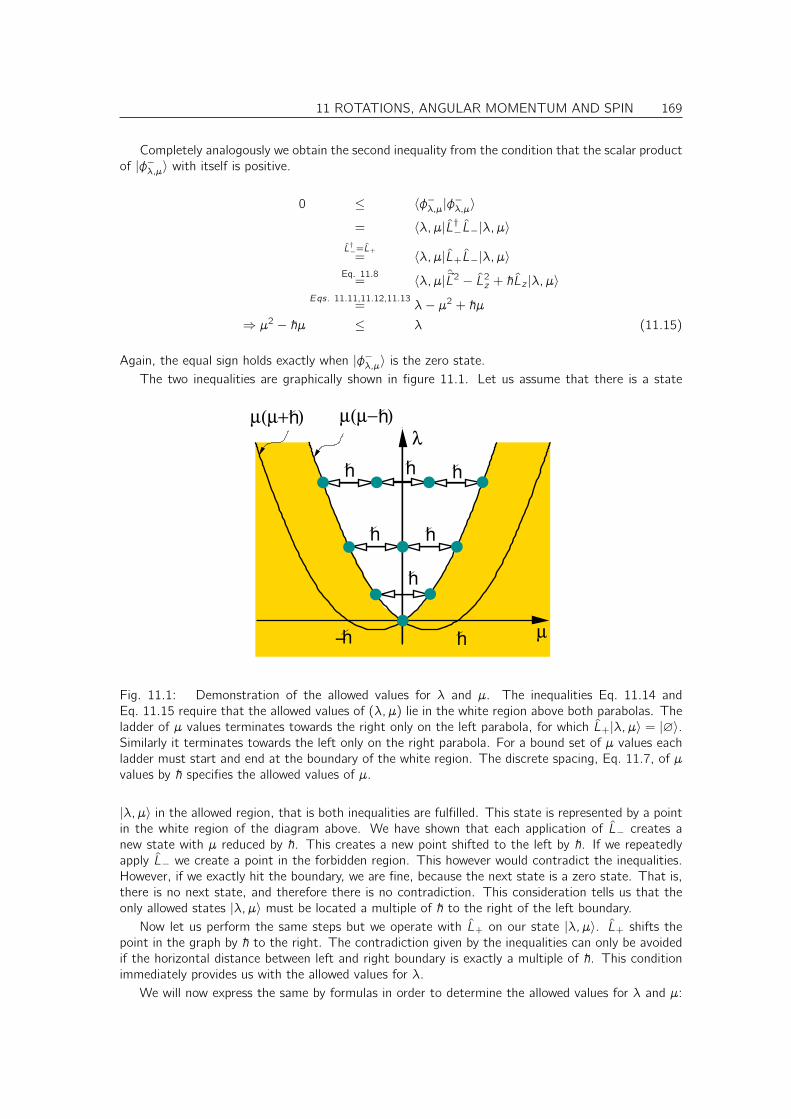
11 ROTATIONS, ANGULAR MOMENTUM AND SPIN 169
Completely analogously we obtain the second inequality from the condition that the scalar productof |φ−λ,µ〉 with itself is positive.
0 ≤ 〈φ−λ,µ|φ−λ,µ〉
= 〈λ, µ|L†−L−|λ, µ〉L†−=L+
= 〈λ, µ|L+L−|λ, µ〉Eq. 11.8
= 〈λ, µ|~L2 − L2z + ~Lz |λ, µ〉
Eqs. 11.11,11.12,11.13= λ− µ2 + ~µ
⇒ µ2 − ~µ ≤ λ (11.15)
Again, the equal sign holds exactly when |φ−λ,µ〉 is the zero state.The two inequalities are graphically shown in figure 11.1. Let us assume that there is a state
hh
hhh
hh
h
hµ(µ+ ) hµ(µ− )
λ
− µ
Fig. 11.1: Demonstration of the allowed values for λ and µ. The inequalities Eq. 11.14 andEq. 11.15 require that the allowed values of (λ, µ) lie in the white region above both parabolas. Theladder of µ values terminates towards the right only on the left parabola, for which L+|λ, µ〉 = |∅〉.Similarly it terminates towards the left only on the right parabola. For a bound set of µ values eachladder must start and end at the boundary of the white region. The discrete spacing, Eq. 11.7, of µvalues by ~ specifies the allowed values of µ.
|λ, µ〉 in the allowed region, that is both inequalities are fulfilled. This state is represented by a pointin the white region of the diagram above. We have shown that each application of L− creates anew state with µ reduced by ~. This creates a new point shifted to the left by ~. If we repeatedlyapply L− we create a point in the forbidden region. This however would contradict the inequalities.However, if we exactly hit the boundary, we are fine, because the next state is a zero state. That is,there is no next state, and therefore there is no contradiction. This consideration tells us that theonly allowed states |λ, µ〉 must be located a multiple of ~ to the right of the left boundary.
Now let us perform the same steps but we operate with L+ on our state |λ, µ〉. L+ shifts thepoint in the graph by ~ to the right. The contradiction given by the inequalities can only be avoidedif the horizontal distance between left and right boundary is exactly a multiple of ~. This conditionimmediately provides us with the allowed values for λ.
We will now express the same by formulas in order to determine the allowed values for λ and µ:

170 11 ROTATIONS, ANGULAR MOMENTUM AND SPIN
The inequalities Eq. 11.14 and Eq. 11.15 require µmin ≤ µ ≤ µmax with
µ2min/max ± ~ µmin/max − λ
Eqs. 11.14,11.15= 0
⇒(µmin/max ±
~2
)2
=
(~2
)2
+ λ
⇒ µmin/max(λ) = ±
~2∓
√(~2
)2
+ λ
The choice of the second sign ∓ determines, whether we choose the inner or the outer branches ofthe two parabola in Fig. 11.1. Because λ is positive, as seen in Fig. 11.1, the negative sign yieldsthe smaller absolute value for µmin/max .
Thus, the the lowest allowed value µmin of µ and the highest allowed value µmax of µ for a givenλ is
µmin(λ) = +
(~2−√
(~2
)2 + λ
)
µmax(λ) = −
(~2−√
(~2
)2 + λ
)(11.16)
Note, that the value of the expression in parenthesis is negative.The requirement that these values differ by a multiple of ~, obtained from Eq. 11.7, yields
µmin − µmax = ~n
where n is an arbitrary non-negative integer. Thus we obtain
−~2
+
√(~2
)2 + λ︸ ︷︷ ︸µmax (λ)
−~2
+
√(~2
)2 + λ︸ ︷︷ ︸−µmin(λ)
= −~ +√~2 + 4λ = ~n
~2(n + 1)2 = ~2 + 4λ
λ = ~2 (n + 1)2 − 1
4= ~2 n
2 + 2n
4= ~2[(
n
2)2 +
n
2]
λ = ~2`(`+ 1)
where we replaced n/2 by `. ` can assume half-integer values ` = 0, 12 , 1, 3
2 , 2, . . .. Thus we have
obtained the eigenvalue spectrum of ~L2.The eigenvalues for Lz are obtained for each ` from
µmin =~2−√
(~2
)2 + λ =~2−√
(~2
)2 + ~2`(`+ 1)
=~2−√~2(`2 + `+
1
4) =~2−√~2(`+
1
2)2 =
~2− ~(`+
1
2)
= −~`
Now we change our notation. Instead of characterizing a state by its eigenvalues λ = ~2`(`+ 1)and µ = ~m as |λ, µ〉, we use the angular quantum numbers ` and m as |`,m〉. Thus we denote theeigenstates of the angular momentum as |λ, µ〉 = |`,m〉.

11 ROTATIONS, ANGULAR MOMENTUM AND SPIN 171
EIGENVALUE SPECTRUM OF THE ANGULAR MOMENTUM
~L2|`,m〉 = |`,m〉~2`(`+ 1)
Lz |`,m〉 = |`,m〉~m
where the quantum numbers ` = 0, 12 , 1, 3
2 , . . . can have any non-negative, half-integer value andm = −`,−`+ 1, . . . , `− 1, `.
h
h
h
h
h
h
L
l(l+1)h
Fig. 11.2: The absolute value of the angular momentum can have the values ~√`(`+ 1). The
eigenvalues of Lz can assume the values ~m, where m = −`,−`+1, . . . , `−1, `. In an eigenstate thevalues of Lz and Ly cannot be determined. It is as if the angular momentum would be precessing.However, the angular momentum does not move, but it simply is delocalized on the circumferenceof the circles shown. Note that L2
x + L2y = ~L2 − L2
z does have sharp values.
Recursion relation for eigenstates
So far we have obtained the eigenvalues and a procedure to create new eigenstates for differenteigenvalues of Lz if one eigenstate is known. However these states are not automatically normalized.Here we want to renormalize the shift operators so that they create normalized states from normalizedstates
〈`,m|L†+L+|`,m〉 = 〈`,m|~L2 − L2z − ~Lz |`,m〉
= 〈`,m|`,m〉(~2`(`+ 1)− ~2m2 − ~2m)
= 〈`,m|`,m〉~2(`(`+ 1)−m(m + 1))
|`,m + 1〉 = L+|`,m〉1
~√`(`+ 1)−m(m + 1)
= L+|`,m〉1
~√
(`−m)(`+m + 1)

172 11 ROTATIONS, ANGULAR MOMENTUM AND SPIN
Similarly we obtain the renormalization for L−
〈`,m|L†−L−|`,m〉 = 〈`,m|~L2 − L2z + ~Lz |`,m〉
= 〈`,m|`,m〉(~2`(`+ 1)− ~2m2 + ~2m)
= 〈`,m|`,m〉~2(`(`+ 1)−m(m − 1))
|`,m − 1〉 = L−|`,m〉1
~√`(`+ 1)−m(m − 1)
= L−|`,m〉1
~√
(`+m)(`−m + 1)
Thus if we know just one eigenstate of the angular momentum for each ` we can construct allothers by the recursion relation above.
Let us summarize here the effect of the angular momentum operators on the basis of eigenstatesof ~L2 and Lz :
~L2|`,m〉 = |`,m〉~2`(`+ 1) (11.17)
Lz |`,m〉 = |`,m〉~m (11.18)
L+|`,m〉 = |`,m + 1〉~√
(`−m)(`+m + 1) (11.19)
L−|`,m〉 = |`,m − 1〉~√
(`+m)(`−m + 1) (11.20)
Because we can express all angular momentum components by Lz , L+, L−, we can derive the matrixelements of any operator composed from angular momenta just from these four relations.4
11.4 Eigenstates of angular momentum: spherical harmonics
In the following we will derive the functional form of the eigenstates of Lz and ~L2, which are calledspherical harmonics.
Let us introduce polar coordinates:
x = r cos(φ) sin(θ)
y = r sin(φ) sin(θ)
z = r cos(θ)
r =√x2 + y2 + z2
θ = acos(z
r)
φ = acos(x√
x2 + y2)sgn(y)
with θ ∈ [0, 2π] and φ ∈ [−π, π]
4The first of these relations is actually redundant, and follows from the remaining three.

11 ROTATIONS, ANGULAR MOMENTUM AND SPIN 173
z
x
y
ϕ
θ
Using Eq. 9.6, we can express the rotation operator S(α)
〈r, θ, φ|S(α)|ψ〉 = 〈r, θ, φ− α|ψ〉︸ ︷︷ ︸ψm(r,θ,φ−α)
(11.21)
which shifts the angle by φ about the z-axis in the form
S(φ)Eq. 11.3
= e−i~ Lzφ (11.22)
If the shift operator is applied to an eigenstate |ψm〉 of the z-component of the angular momentumLz with eigenvalue ~m, we obtain
S(α)|ψm〉Eq. 11.22
= e−i~ Lzα|ψm〉
Lz |ψm〉=|ψm〉~m= |ψm〉e−imα
〈r, θ, φ|S(α)|ψm〉Eq. 11.21
= 〈r, θ, φ− α|ψm〉 = 〈r, θ, φ|ψm〉e−imα
setting first φ = 0 and then α = −φ we obtain
ψm(r, θ, φ) = ψm(r, θ, 0)eimφ
Thus we obtained the φ-dependence of the angular momentum. This works fine for integer angularmomentum. For a half-integerm, the wave function changes its sign for a full turn, because eiπ = −1.Hence they cannot be associated with a single valued wave function ifm is not an integer. Half-integerangular momenta are associated to spin, which we will discuss later.
The θ-dependence can be obtained from L−Y`,−` = 0 andL+Y`,m = Y`,m+1~
√`(`+ 1)−m(m − 1). Here we only summarize the main results.
The full eigenstates are[34]
Y`,m(θ, φ) =
√2`+ 1
4π
(`−m)!
(`+m)!Pm` (cos θ)eimφ (11.23)
The Pm` are called associated Legendre polynomials defined as
P|m|` (u) = (−1)m
√1− u2
|m| d |m|
du|m|P`(u). (11.24)
P−|m|` (u) = (−1)m
(`− |m|)!
(`+ |m|)!P|m|` (u) (11.25)

174 11 ROTATIONS, ANGULAR MOMENTUM AND SPIN
with the help of the Legendre polynomials
P`(u) =1
2``!∂`u(u2 − 1)` (11.26)
Numerically, associated Legendre polynomials are be evaluated by efficient recursion relations. Mostrecursion relations amplify numerical errors, rendering them useless. A recursion relation for asso-ciated Legendre polynomials that works is found in the “Numerical Recipes”[34]. It is in generaladvisable to consult a book on numerical mathematics such as the “Numerical Recipes”, before eval-uating special functions on the computer, as they often pose substantial difficulties that are easilyoverlooked.
Y`,m(~r) Y`,m(θ, φ)
Y0,0
√1
4π
√1
4π
Y1,−1
√3
8πx−iyr
√3
8π sin θe−iφ
Y1,0
√3
4πzr
√3
4π cos(θ)
Y1,1 −√
38π
x+iyr −
√3
8π sin θeiφ
Y2,−2
√15
32π(x2−y2)−ixy
r2
√15
32π sin2 θe−2iφ
Y2,−1
√158π
xz−iyzr2
√158π sin θ cos θe−iφ
Y2,0
√5
16π3z2−r2
r2
√5
16π (3 cos2 θ − 1)
Y2,1 −√
158π
xz+iyzr2 −
√158π sin θ cos θeiφ
Y2,2
√15
32π(x2−y2)+ixy
r2
√15
32π sin2 θe2iφ
Table 11.1: Spherical harmonics Y`,m in Cartesian and polar coordinates. Polar coordinates aredefined as x = r sin θ cosφ, y = r sin θ sinφ and z = r cos θ. Source: Jackson: Electrodynamics andAtkins[4].
Often the real spherical harmonics are used, which are fully real, but are not eigenstates of Lz .We denote them with the symbol Y . For m = 0 real and complex spherical harmonics are identical.For m 6= 0 we use the following definition.
Y`,|m| =1√2
(Y`,|m| + (−1)mY`,−|m|
)=√
2Re[Y`,m]
Y`,−|m| = −i√2
(Y`,|m| − (−1)mY`,−|m|
)=√
2Im[Y`,m]
Note that the real spherical harmonics are still eigenstates to ~L2, but they are no eigenstates of LzThe following is a list of real spherical harmonics from which the complex spherical harmonics are
readily obtained. Here the real spherical harmonics are identified by a running index n = `2 + `+m

11 ROTATIONS, ANGULAR MOMENTUM AND SPIN 175
s Y1 Y0
√1
4π
px Y21√2
(Y1,1 − Y1,−1)√
34π
xr
pz Y3 Y1,0
√3
4πzr
py Y4−i√
2(Y1,1 + Y1,−1)
√3
4πyr
dx2−y2 Y51√2
(Y2,2 + Y2,−2)√
1516π
x2−y2
r2
dxz Y61√2
(Y2,1 − Y2,−1)√
6016π
xzr2
d3z2−r2 Y7 Y2,0
√5
16π3z2−r2
r2
dyz Y8−i√
2(Y2,1 + Y2,−1)
√60
16πyzr2
dxy Y9−i√
2(Y2,2 − Y2,−2)
√60
16πxyr2
|Y l,m( )
|ϕ
ϕ
x
y
Fig. 11.3: Representation of real spherical harmonics (cos(ϕ)) in polar coordinates. For a givendirection defined by the angles θ, φ, a vector with a length equal to the absolute value of the amplitudeof the real spherical harmonics points from the origin to the graph of the curve. Because this graphdoes not distinguish the different signs of the function, they are indicated by coloring the lobes withpositive and negative values differently. Note that spherical harmonics defined as eigenstates of theangular momentum ~L2 and Lz are complex, so that real and imaginary part of a spherical harmonicsmust be drawn separately. Real spherical harmonics are not eigenstates of Lz , but they are alreadyreal.

176 11 ROTATIONS, ANGULAR MOMENTUM AND SPIN
spx py pz
dxy dxz dyzdx2y2 dz2
Fig. 11.4: Real spherical harmonics: The graphical representation refers to a surface | 1|r | Y`,m(~r)| = 1.
That is for every angle the distance of the surface from the origin is equal to the value of the sphericalharmonic. Typically the lobes are colored differently to distinguish regions with positive and negativesign. The motivation for these plots is the representation of atomic orbitals, which are eigenstatesof angular momentum and have the form R(|r |)Y`,m(~r). If we plot a surface where the orbital hasone value c in one color, and another surface for a value −c with another color, we obtain similarlylooking lobes.
11.5 Spin
An important result of the algebraic derivation of the spectrum of the angular momentum is theexistence of states with half-integer m quantum number. There is no single valued wave function inreal space that is an eigenstate to a non-integer m so that Lz |ψ〉 = |ψ〉~m. Therefore, we could nothave found these eigenvalues by trying to solve the differential equation in real space. The way outis to treat spin algebraically.
In the following we concentrate on eigenstates with ` = 12 , which we also call spin 1
2 eigenstates.States with other spin values ` can be represented analogously.
Let us introduce a basis of spin eigenstates, namely | ↑〉def= |1
2︸︷︷︸`
,1
2︸︷︷︸m
〉 and | ↓〉def= | 12 ,−12 〉 defined
by
Lz | ↑〉 = | ↑〉~2
Lz | ↓〉 = | ↓〉(−~2
)
so that (〈↑ |Lz | ↑〉 〈↑ |Lz | ↓〉〈↓ |Lz | ↑〉 〈↓ |Lz | ↓〉
)=~2
(1 0
0 −1
)

11 ROTATIONS, ANGULAR MOMENTUM AND SPIN 177
Now we use
L+|`,m〉 = |`,m + 1〉~√`(`+ 1)−m(m + 1)
L−|`,m〉 = |`,m − 1〉~√`(`+ 1)−m(m − 1)
with ` = 12 and m = ± 1
2 to express the action of the ladder operators L+ and L− in terms of thesebasis functions
L−| ↑〉 = | ↓〉~; L−| ↓〉 = 0
L+| ↑〉 = 0; L+| ↓〉 = | ↑〉~
(〈↑ |L−| ↑〉 〈↑ |L−| ↓〉〈↓ |L−| ↑〉 〈↓ |L−| ↓〉
)= ~
(0 0
1 0
)(〈↑ |L+| ↑〉 〈↑ |L+| ↓〉〈↓ |L+| ↑〉 〈↓ |L+| ↓〉
)= ~
(0 1
0 0
)
Using Lx = 12 (L+ + L−) and Ly = 1
2i (L+ − L−) we obtain the remaining two components of theangular momentum (
〈↑ |Lx | ↑〉 〈↑ |Lx | ↓〉〈↓ |Lx | ↑〉 〈↓ |Lx | ↓〉
)=~2
(0 1
1 0
)(〈↑ |Ly | ↑〉 〈↑ |Ly | ↓〉〈↓ |Ly | ↑〉 〈↓ |Ly | ↓〉
)=~2
(0 −ii 0
)
Thus we can write
Li
(ψ↑
ψ↓
)=~2σi
(ψ↑
ψ↓
)
where Ψ↑ = 〈↑ |Ψ〉 and Ψ↓ = 〈↓ |Ψ〉 are vector components of a state |Ψ〉 in the basis of eigenstatesto Lz , and where the σi are the so-called Pauli Matrices
σx =
(0 1
1 0
); σy =
(0 −ii 0
); σz =
(1 0
0 −1
)
that we have already learned about in the section on the two state system.Most particles have an angular momentum that is not related to its “trajectory”. One interprets
it as the rotation of a particle about its axis. A spin 12 particle of this type is the electron. It is
described by a double valued spatial wave function (Ψ↑(r),Ψ↓(r)), that is able to describe both itsposition and angular momentum coordinates.
The spin at a certain point is obtained from a two-component wave function by
Si(r) =~2
(Ψ∗↑(r)
Ψ∗↓(r)
)σi
(Ψ↑(r)
Ψ↓(r)
)
Sx(r) =~2
(Ψ∗↑(r)Ψ↓(r) + Ψ∗↓(r)Ψ↑(r)
)= ~Re[Ψ∗↑(r)Ψ↓(r)]
Sy (r) =~2i
(Ψ∗↑(r)Ψ↓(r)−Ψ∗↓(r)Ψ↑(r)
)= ~Im[Ψ∗↑(r)Ψ↓(r)]
Sz(r) =~2
(Ψ∗↑(r)Ψ↑(r)−Ψ∗↓(r)Ψ↓(r)
)

178 11 ROTATIONS, ANGULAR MOMENTUM AND SPIN
The particle density is obtained as the sum of the squared components.
n(r) =(
Ψ∗↑(r)Ψ↑ + Ψ∗↓(r)Ψ↓(r))
Often the wave functions are constrained to have exclusively either only a spin-up component orexclusively a spin-down component. Then the states are eigenstates to Sz = ~
2σz .
11.6 Addition of angular momenta
Let us consider two electrons orbiting in an atom. Obviously this is a rotationally invariant problem,and therefore the angular momentum must be a quantum number. However, if the particles interact,they can exchange angular momentum between themselves, as only the total angular momentum isconserved.
We can describe the two electrons by their individual angular momenta ~L1 and ~L2, where ~L1 actsonly on the coordinates and momenta of the first electron and ~L2 acts only on the coordinates andmomenta of the second atom. Examples:
• For example if the two electrons are described by a two-particle wave functions Ψ(~r1, ~r2), theangular momentum acting on the first particle would be
〈~r1, ~r2|~L1|Ψ〉 =: ~L1Ψ(~r1, ~r2) =~i~r1 × ~∇~r1 Ψ(~r1, ~r2)
〈~r1, ~r2|L2|Ψ〉 =: L2Ψ(~r1, ~r2) =~i~r2 × ~∇~r2 Ψ(~r1, ~r2)
The total angular momentum is denoted as
~Jdef= ~L1 + ~L2
Its eigenvalues will be denoted by j = `J and jz = mJ .
• Similarly we can consider a single particle with spin orbiting an atom. In this case, the totalangular momentum has the form
~J = ~L+ ~S
where ~L is the orbital angular momentum and ~S is the spin of the particle. In two-componentspinor representation the total angular momentum has the form
~J = ~r × ~p 111 + 1~2~σ
= ~r ×~i~∇
(1 0
0 1
)+~2~σ
This is a difficult but very instructive example: We have operators, denoted by a hat, “ ˆ ”, thatacts on states that correspond square integrable complex functions in the three-dimensionalcoordinate space and those that act on the two-dimensional spin states. The complicationcomes from the complex nature of the Hilbert space for that system. This Hilbert space is aproduct of a two-dimensional Hilbert space, describing the spin, and the Hilbert space of wavefunctions in three-dimensional coordinate space. A basis state in that space is
|~r , σ〉
where σ can have the values ↑ or ↓. The two dimensional matrices act on the second variable,whereas the differential operators act on the first variable.

11 ROTATIONS, ANGULAR MOMENTUM AND SPIN 179
When the electrons interact, each electron does not have a conserved angular momentum. Thetotal angular momentum ~J = ~L1 + ~L2 is still conserved. Hence we are looking for eigenstates of ~Jzand ~J2. Note that the eigenvalues for ~J2 and Jz are denoted by ~j(j + 1) and ~jz respectively.
The question we address in the following is, how we transform between these two sets of eigen-states.
We start out with a basis of angular momentum eigenstates for each electron individually
~L21|`1, m1, `2, m2〉 = |`1, m1, `2, m2〉~2`1(`1 + 1)
~L22|`1, m1, `2, m2〉 = |`1, m1, `2, m2〉~2`2(`2 + 1)
L1,z |`1, m1, `2, m2〉 = |`1, m1, `2, m2〉~m1
L2,z |`1, m1, `2, m2〉 = |`1, m1, `2, m2〉~m2
L1,−|`1, m1, `2, m2〉 = |`1, m1 − 1, `2, m2〉~√
(`1 +m1)(`1 −m1 + 1)
L2,−|`1, m1, `2, m2〉 = |`1, m1, `2, m2 − 1〉~√
(`2 +m2)(`2 −m2 + 1)
L1,+|`1, m1, `2, m2〉 = |`1, m1 + 1, `2, m2〉~√
(`1 −m1)(`1 −m1 + 1)
L2,+|`1, m1, `2, m2〉 = |`1, m1, `2, m2 + 1〉~√
(`2 −m2)(`2 −m2 + 1)
Let us express ~J2 by the angular momenta of individual particles ~L1 and ~L2
~J2 = ~L21 + 2~L1
~L2 + ~L22
= ~L21 + ~L2
2 + 2[L1,x L2,x + L1,y L2,y + L1,z L2,z
]= L2
1 + L22 + 2L1,zL2,z +
[L1,+L2,− + L1,−L2,+
]Apparently the states are not eigenstates of the total angular momentum. To show this let us
apply Jz and J2 to the eigenstates of L1 and L2.
Jz |`1, m1, `2, m2〉 = ~(m1 +m2)|`1, m1, `2, m2〉J2|`1, m1, `2, m2〉 = ~2[`1(`1 + 1) + `2(`2 + 1) + 2m1m2]|`1, m1, `2, m2〉
+ |`1, m1 + 1, `2, m2 − 1〉× ~2
√[`1(`1 + 1)−m1(m1 + 1)][`2(`2 + 1)−m2(m2 − 1)]
+ |`1, m1 − 1, `2, m2 + 1〉× ~2
√[`1(`1 + 1)−m1(m1 − 1)][`2(`2 + 1)−m2(m2 + 1)]
In order to find an eigenstate of J2 we need to superimpose the states with a given `1, `2 andm = m1 +m2.
The new basis will have the eigenvalues
J2|`1, `2, `,m〉 = ~2`(`+ 1)|`1, `2, `,m〉Jz |`1, `2, `,m〉 = ~m|`1, `2, `,m〉L2
1|`1, `2, `,m〉 = ~2`1(`1 + 1)|`1, `2, `,m〉L2
1|`1, `2, `,m〉 = ~2`1(`1 + 1)|`1, `2, `,m〉
which is a definition of the basis functions |`1, `2, `,m〉.The general form of the basis functions is
|`1, `2, `,m〉 =
min(`1,`2)−m/2∑i=−min(`1,`2)−m/2
|`1,m
2+ i , `2,
m
2− i〉ci

180 11 ROTATIONS, ANGULAR MOMENTUM AND SPIN
where the coefficients ci also depend on `1, `2, `,m. The coefficients ci = 〈`1, m1, `2, m2|`1, `2, `,m〉with i = m1−m2
2 , which also depend on `1, `2, m, ` are called Clebsch-Gordan coefficients, Wigneror vector coupling coefficients.
They are fairly complex so that we will not evaluate them here.Editorial remark: Work on this section. Also include pictorial description of vector addition
components as in Atkins
11.7 Products of spherical harmonics
Extremely useful is the product rule of spherical harmonics.
GAUNT COEFFICIENTS
The Gaunt coefficients[35] are defined as
G`′′,m′′
`,m,`′,m′def=
∫dΩ Y ∗`′′,m′′(~r)Y`,m(~r)Y`′,m′(~r) (11.27)
The Gaunt coefficients can be used to express the product of two spherical harmonics by a sum ofsingle spherical harmonics, called the Gaunt series.
Y`,m(~r)Y`′,m′(~r) =∑`′′,m′′
G`′′,m′′
`,m,`′,m′Y`′′,m′′(~r)
Note that the definition of Gaunt coefficients is not uniform, and I have seen definitions with anadditional factor of
√4π (Cohen Tannoudji). In order to confirm numerically of the definition agrees
with the one given above, simply test the coefficients G0,0`,m,`,m = 1√
4π. This rule can be derived, from
knowing that Y`,m = 1√4π.
The product rule is for example needed to express the particle density of an atom in sphericalharmonics, if the wave function are given as radial function times spherical harmonics. If Ψn(~r) =Rn(|~r |)Y`,m(~r), we obtain
ρ(~r) = qΨ∗(~r)Ψ(~r) =∑`′′,m′′
G`′′,m′′
`,−m,`,m|R(|~r |)|2 Y`′′,m′′(~r)
Here, we used the property that Y ∗`,m(~r) = Y`,−m(~r), which is obtained from the definition Eq. 11.23with the help of Eq. 11.25.
The Gaunt coefficients are closely related to the Clebsch-Gordan coefficients:
G`,m`1,m1,`2,m2= (−1)m2
√(2`1 + 1)(2`2 + 1)
4π(2`+ 1)〈`1, 0, `2, 0|`1, `2, `, 0〉〈`1, m1, `2,−m2|`1, `2, `,m〉
In the following we sketch how these coefficients are derived: We start out with a two particlewave function, which depends on the positions ~r1 and ~r2 of the two particles.
〈r1, r2|`1, m1, `2, m2〉 = Y`1,m1 (~r1)Y`2,m2 (~r2)
〈r1, r2|`1, `2, `,m〉 = Φ(~r1, ~r2)
We can relate Φ to the products of two wave functions using the Clebsch Gordan coefficients.
〈~r1, ~r2|`1, m1, `2, m2〉 =∑`,m
〈~r1, ~r2|`1, `2, `,m〉〈`1, `2, `,m|`1, m1, `2, m2〉
Y`1,m1 (~r1)Y`2,m2 (~r2) =∑`,m
Φ`1,`2,`,m(~r1, ~r2)〈`1, `2, `,m|`1, m1, `2, m2〉

11 ROTATIONS, ANGULAR MOMENTUM AND SPIN 181
and therefore also
Y`1,m1 (~r)Y`2,m2 (~r) =∑`,m
Φ`1,`2,`,m(~r ,~r)〈`1, `2, `,m|`1, m1, `2, m2〉
It can be shown that Φ(~r ,~r) is proportional to a spherical harmonic itself. Once that is shown,we only need to work out the normalization constants.
Let us show that F`1,`2,`,m(~r) = Φ`1,`2,`,m(~r ,~r) is a spherical harmonic. Therefore, we apply anangular momentum operator to F : Using product and chain rule we relate the derivatives of F . Wecan consider ~r1 and ~r2 to be functions of r namely ~r1(~r) = ~r and ~r2(~r) = ~r .
~r1(~r) = ~r
~r2(~r) = ~r
~r ×∇F (~r) = ~r ×∇Φ(~r1(~r), ~r2(~r))
= [~r ×∇1 + ~r ×∇2]Φ(~r1(~r), ~r2(~r))
= [~r1 ×∇1 + ~r2 ×∇2]Φ(~r1(~r), ~r2(~r))
LF (~r) = [~L1 + ~L2]Φ(~r ,~r)
where ~L1 acts only on the first argument and ~L2 on the second.Because Φ(~r1, ~r2) is an eigenstate of angular momentum (~L1 + ~L2)Φ(~r1, ~r2) = Φ(~r1, ~r2)~2`(`+ 1)
and (~L1,z +~L2,z)Φ(~r1, ~r2) = Φ(~r1, ~r2)~m we find that also F (r) is an eigenstate of angular momentumLz and L2,
Lz |F 〉 = ~m|F 〉L2|F 〉 = ~2`(`+ 1)|F 〉
which implies that they are related to spherical harmonics.The derivation of the remaining coefficients can be found in Cohen-Tannoudji[3].
11.8 Recommended exercises
1. Rotator: Exercise 16.5 on p. 238. (Not ready)

182 11 ROTATIONS, ANGULAR MOMENTUM AND SPIN

Chapter 12
Atoms
12.1 Radial Schrödinger equation
Let us consider a particle in a spherically symmetric potential
[ ~p2
2m+ V (|~r |)
]|ψ〉 = |ψ〉E
Editor: Include hats to distinguish numbers from operatorsWe introduce the radial momentum pr = 1
|r |(~r~r) and obtain an expression that contains radialand angular momenta separately.
[ 1
2m
(1
rp2r r +
1
r2L2)
+ V (r)]|ψ〉 = |ψ〉E
where r = |~r |. Note, that[8]
1
rp2r r =
1
r2pr
(r2pr
)
183
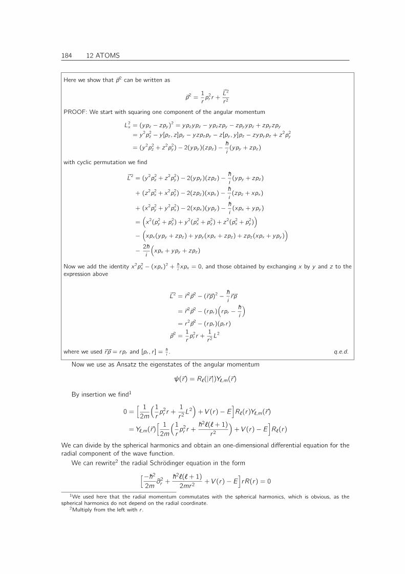
184 12 ATOMS
Here we show that ~p2 can be written as
~p2 =1
rp2r r +
~L2
r 2
PROOF: We start with squaring one component of the angular momentum
L2x = (ypz − zpy )2 = ypzypz − ypzzpy − zpyypz + zpyzpy
= y 2p2z − y [pz , z ]py − yzpzpy − z [py , y ]pz − zypypz + z2p2
y
= (y 2p2z + z2p2
y )− 2(ypy )(zpz)− ~i
(ypy + zpz)
with cyclic permutation we find
~L2 = (y 2p2z + z2p2
y )− 2(ypy )(zpz)− ~i
(ypy + zpz)
+ (z2p2x + x2p2
z )− 2(zpz)(xpx)− ~i
(zpz + xpx)
+ (x2p2y + y 2p2
x )− 2(xpx)(ypy )− ~i
(xpx + ypy )
=(x2(p2
y + p2z ) + y 2(p2
x + p2z ) + z2(p2
x + p2y ))
−(xpx(ypy + zpz) + ypy (xpx + zpz) + zpz(xpx + ypy )
)− 2~
i
(xpx + ypy + zpz)
Now we add the identity x2p2x − (xpx)2 + ~
ixpx = 0, and those obtained by exchanging x by y and z to the
expression above
~L2 = ~r 2~p2 − (~r ~p)2 − ~i~r ~p
= ~r 2~p2 − (rpr )(rpr −
~i
)= r 2~p2 − (rpr )(pr r)
~p2 =1
rp2r r +
1
r 2L2
where we used ~r ~p = rpr and [pr , r ] = ~i. q.e.d.
Now we use as Ansatz the eigenstates of the angular momentum
ψ(~r) = R`(|~r |)Y`,m(~r)
By insertion we find1
0 =[ 1
2m
(1
rp2r r +
1
r2L2)
+ V (r)− E]R`(r)Y`,m(~r)
= Y`,m(~r)[ 1
2m
(1
rp2r r +
~2`(`+ 1)
r2
)+ V (r)− E
]R`(r)
We can divide by the spherical harmonics and obtain an one-dimensional differential equation for theradial component of the wave function.
We can rewrite2 the radial Schrödinger equation in the form[−~2
2m∂2r +~2`(`+ 1)
2mr2+ V (r)− E
]rR(r) = 0
1We used here that the radial momentum commutates with the spherical harmonics, which is obvious, as thespherical harmonics do not depend on the radial coordinate.
2Multiply from the left with r .
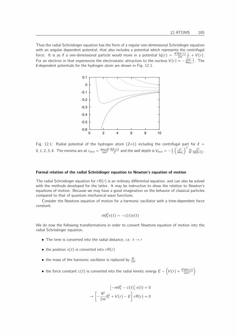
12 ATOMS 185
Thus the radial Schrödinger equation has the form of a regular one-dimensional Schrödinger equationwith an angular dependent potential, that also includes a potential which represents the centrifugalforce. It is as if a one-dimensional particle would move in a potential V`(r) = ~2`(`+1)
2m1r2 + V (r).
For an electron in that experiences the electrostatic attraction to the nucleus V (r) = − Ze2
4πε0
1r . The
`-dependent potentials for the hydrogen atom are shown in Fig. 12.1.
-0.6
-0.5
-0.4
-0.3
-0.2
-0.1
0
0.1
0 2 4 6 8 10
Fig. 12.1: Radial potential of the hydrogen atom (Z=1) including the centrifugal part for ` =
0, 1, 2, 3, 4. The minima are at rmin = 4πε0~2
me2
`(`+1)Z and the well depth is Vmin = − 1
2
(e2
4πε0
)2m~2
Z2
2`(`+1) .
Formal relation of the radial Schrödinger equation to Newton’s equation of motion
The radial Schrödinger equation for rR(r) is an ordinary differential equation, and can also be solvedwith the methods developed for the latter. It may be instructive to show the relation to Newton’sequations of motion. Because we may have a good imagination on the behavior of classical particlescompared to that of quantum mechanical wave functions.
Consider the Newtons equation of motion for a harmonic oscillator with a time-dependent forceconstant.
m∂2t x(t) = −c(t)x(t)
We do now the following transformations in order to convert Newtons equation of motion into theradial Schrödinger equation.
• The time is converted into the radial distance, i.e. t → r
• the position x(t) is converted into rR(r)
• the mass of the harmonic oscillator is replaced by ~2
2m
• the force constant c(t) is converted into the radial kinetic energy E −(V (r) + ~2`(`+1)
2mr2
)[−m∂2
t − c(t)]x(t) = 0
→[−~2
2m∂2r + V (r)− E
]rR(r) = 0

186 12 ATOMS
Boundary conditions at the origin
The main difference of the radial Schrödinger equation to the one-dimensional Schrödinger equationare the boundary conditions at the origin r = 0. We proceed here with an expansion of R in powersof r , that is
R(r) =∑j
aj rj
We maintain only the leading order in r of the potential, that is V (r) = Crα(
1 +O(r)).
0 =[−~2
2m∂2r +~2`(`+ 1)
2mr2+ Crα − E
]∑j
aj rj+1
=∑j
[−~2
2mj(j + 1)aj r
j−1 +~2`(`+ 1)
2maj r
j−1 + Caj rα+j+1 − Eaj r j+1
]=∑j
r j−1[−~2
2m
(j(j + 1)− `(`+ 1)
)aj + Caj−α−2 − Eaj−2
]which results in a recursion relation for the coefficients
0 =−~2
2m
(j(j + 1)− `(`+ 1)
)aj + Caj−α−2 − Eaj−2
= (j − `)(j + `+ 1)aj −2mC
~2aj−α−2 +
2mE
~2aj−2
aj =1
(j − `)(j + `+ 1)
(2mC
~2aj−α−2 −
2mE
~2aj−2
)(12.1)
Let us consider the case where
• α = −1. This case is important for atoms, because the electrostatic potential of an electronthat experiences the Coulomb attraction of the nucleus is of this form V (r) = − Ze2
4πε0r. We
need to consider a solution for which aj<j0 = 0. In Eq. 12.1, aj0 can only be nonzero, if thedenominator vanishes, which determines the possible values of j0.
(j0 − `)(j0 + `+ 1)aj0 = 0⇒ j0 = ` or j0 = −`− 1
The solution j0 = −` − 1 can be discarded because it will be irregular at the origin and notnormalizable. The coefficient aj0 is arbitrary and will be determined by the normalization con-dition.
In order to obtain the next term in the expansion, we insert this result into Eq. 12.1 forj = j0 + 1 = `+ 1
a`+1 =mC
~2
1
`+ 1a`
Thus the radial wave function behaves near the origin as
Rr (r) = A[
1 +mC
~2(`+ 1)r +O(r2)
]r `
and is not differentiable for ` = 0, which is a consequence of the Coulomb singularity. Thiskink is not energy dependent, while the higher order terms would depend explicitly on energy.
For the “hydrogen atom” with atomic number Z we obtain C = −Ze2/(4πε0) and a recursionrelation with k = j − `
aj =1
(j − `)(j + `+ 1)
(−
2mZe2
4πε0~2aj−1 +
2mE
~2aj−2
)= 0
ak<0 = 0

12 ATOMS 187
so that
Rr (r) = a0
[1−
mZe2
4πε0~2(`+ 1)r +O(r2)
]r `
Note, that the kink is independent of the energy.
• α = 0 which describes a continuous potential. The term proportional r `+1 vanishes, and thesecond radial function behaves like
Rr (r) = A[
1 +O(r2)]r `
The recursion relation Eq. 12.1 for the coefficients could be used to determine a Taylor expansionof R(r) to arbitrary high order. More accurate results are obtained, when one uses the Taylorexpansion to obtain value and derivative at a point close to the nucleus and to use these values asinitial conditions for a numerical solution of the Schrödinger equation.
12.2 The Hydrogen Atom
The potential for the hydrogen atom is
V (~r) = −Ze2
4πε0|r |
where Z is the atomic number, e is the elementary charge, and ~r is the position relative to the nuclearsite. The radial potentials including the centrifugal term are shown in Fig. 12.1.
[−~2
2me∂2r +~2`(`+ 1)
2mer2−
Ze2
4πε0r− E
]rR(r) = 0
Hartree atomic units
Let us simplify the equation by introducing dimensionless quantities. We multiply with me/~2 andintroduce a length unit and an energy unit so that the equation is dimensionally consistent.[
−∂2r +
`(`+ 1)
r2+
2meZe2
4πε0~2
1
r−
2meE
~2
]rR(r) = 0[
−1
2∂2r +
`(`+ 1)
2r2+
Z
a0r−
E
E0a20
]rR(r) = 0[
−1
2∂2y +
`(`+ 1)
2y2+Z
y−E
E0
]yR(ya0) = 0 (12.2)
Thus we have defined a length scale, the Bohr radius a0, and an energy scale, the Hartree E0 = H.
Definition 12.1 BOHR RADIUS
a0 =4πε0~2
mee2(12.3)
The Bohr radius is the length unit of the Hartree atomic unit system. It corresponds to the radius ofa classical electron circling a proton at the ground state energy of the quantum mechanical hydrogenatom.

188 12 ATOMS
Definition 12.2 HARTREE
H =~2
mea20
=mee
4
(4πε0~)2(12.4)
The Hartree is the energy unit of the Hartree atomic unit system. One Hartree is twice the bindingenergy of an electron in the hydrogen atom.
In this way we can define a new system of units, the so-called Hartree atomic units.
Definition 12.3 HARTREE ATOMIC UNITSThe Hartree atomic units are defined by
~ = me = e = 4πε0 = 1
where me is the electron mass, e is the elementary charge, and ε0 is the dielectric constant of thevacuum.The Hartree atomic unit system is commonly used for atomic and molecular physics. Unlike the officialSI unit system, Hartree atomic units are defined entirely by measurable fundamental quantities.
• the length unit of the Hartree atomic unit system is the Bohr radius, which corresponds to theradius of the classical orbit of an electron in the hydrogen atom.
• the energy unit is the Hartree, which is twice the binding energy of a hydrogen atom.
Instead of using the symbols a0, H, etc. one often uses a.u. which stands for “atomic unit” in general.Note that there are two atomic unit systems. The so-called Rydberg atomic unit system is different.This leads to confusion, because often it is not spelled out, which of the two atomic unit systems ismeant.
In Hartree atomic units, the Schrödinger equation of an electron in the Coulomb potential of thenucleus has the form (
−1
2∇2 −
Z
r− E
)|Ψ〉 = 0
The values of the fundamental constants and the conversion factors can be found in the book“Quantities, Units and Symbols in Physical Chemistry” [36] or on the web[37, 38].
Bound wave functions
Before we solve Eq. 12.2 let us investigate its qualitative behavior, which will guide us to useful ansatzfor the solution. We can simplify the differential equation, if we consider the two limits r → 0 andr →∞
• For r → 0 we can use the Power series expansion, which tells us that the wave function at theorigin is proportional to r `.
• For r →∞ we can ignore the potential and the centrifugal term. Thus the differential equationbecomes independent of Z and `. We obtain with y = r/a0[
−1
2∂2y −
E
H
]yR(ya0) ≈ 0
which can easily be solved. The solution has the form
R(ya0) ∼1
ye−√
2 EHy
12 ATOMS 189
The wave function decays exponentially with the decay governed by the energy. For boundstates the wave functions decay exponentially, while they oscillate for positive energies. Herewe only consider the bound states.
These considerations suggest an Ansatz of the form
R(ya0) = F (y)y `e−λx
where
λdef=
√2E
H(12.5)
The goal is now to determine the function F (y)
We insert this Ansatz into the radial Schrödinger equation. Eq. 12.2:[−
1
2∂2y +
`(`+ 1)
2y2−Z
y−E
H
]F (y)y `+1e−λy = 0 .
We use
∂yy`+1e−λy = y `+1e−λy [
`+ 1
y− λ+ ∂y ]
⇒ ∂2y y
`+1e−λy = y `+1e−λy [`+ 1
y− λ+ ∂y ][
`+ 1
y− λ+ ∂y ]
= y `+1e−λy
[(`+ 1
y− λ
)2
+ ∂y
(`+ 1
y− λ
)+
(`+ 1
y− λ
)2
∂y + ∂2y
]
= y `+1e−λy[
(`+ 1
y− λ)2 −
`+ 1
y2+ 2[
`+ 1
y− λ]∂y + ∂2
y
]= y `+1e−λy
[∂2y + 2[
`+ 1
y− λ]∂y +
`(`+ 1)
y2− 2λ
`+ 1
y+ λ2
]and insert into the radial Schrödinger equation Eq. 12.2[
∂2y + 2[
`+ 1
y− λ]∂y −
2
y
(λ(`+ 1)− Z
)+(2E
H+ λ2
)︸ ︷︷ ︸
=0
]F (y) = 0
⇒[y∂2
y + 2[`+ 1− λy ]∂y − 2(λ(`+ 1)− Z
)]F (y) = 0 (12.6)
This differential equation is a special case of the general associated Laguerre differential equation.(x∂2
x + (k + 1− x)∂x + n)L(k)n (x) = 0
where k, n are integers. The solutions are the so-called associated Laguerre Polynomials
L(k)n (x) =
exx−k
n!
dn
dxne−xxn+k
This can be used if one find the corresponding tables. A useful source is the Book of Abramowitzand Stegun[39].
However, here we want to investigate how such a problem can be solved directly: We make apower-series Ansatz for F (y) =
∑j ajy
j in Eq. 12.6.∑j
[j(j − 1)ajy
j−1 + 2(`+ 1)jajyj−1 − 2λjajy
j − 2(λ(`+ 1)− Z
)ajy
j]
= 0
∑j
[j(j − 1) + 2(`+ 1)j ] ajyj−1 −
∑j
[2λj +
(λ(`+ 1)− Z
)]ajy
j = 0
∑j
[(j + 1)j + 2(`+ 1)(j + 1)] aj+1 −∑j
[2λj +
(λ(`+ 1)− Z
)]aj
y j = 0

190 12 ATOMS
Because the identity holds for all values of y , it must also hold in every power of y .3 If we collectall terms that are proportional to a certain power of y , namely y j−1, we obtain
j(j + 1)aj+1 + 2(`+ 1)(j + 1)aj+1 − 2λjaj − 2(λ(`+ 1)− Z
)aj = 0
⇒(j(j + 1) + 2(`+ 1)(j + 1)
)aj+1 − 2
(λj + λ(`+ 1)− Z
)aj = 0,
which provides us with a recursion relation for the coefficients aj
aj+1 = 2λ(j + `+ 1)− Z
(j + 1)(j + 2`+ 2)aj (12.7)
The power series can start following that index, where the denominator vanishes that is with j = 0or j = −(2` + 1). The second choice leads to the irregular solution. The irregular solution has asingularity at the origin. The resulting wave function would obey the Schrödinger equation everywhere,except at the origin.Therefore, the irregular solution must be excluded. Thus the power series startswith jmin = 0, which leads to the regular solution.
The power series also has an upper end, where the numerator of Eq. 12.7 vanishes: The powerseries expansion finishes, if there is an integer jmax so that
0 = λ(jmax + `+ 1)− Z ⇒ jmax = −`− 1 +Z
λ
jmax must itself be a positive integer, because otherwise the power series does not terminate.(Some further calculations are required to show that such solutions lead to exponentially increasingfunctions that cannot be normalized.4 )
The requirement that jmax is an integer, determines the allowed values for λ. For jmax we obtain
λjmax =Z
jmax + `+ 1(12.8)
We introduce a new variable the so-called principal quantum number
n = jmax + `+ 1 (12.9)
Now we take the definition of λ, Eq. 12.5, resolve it for the energy,
E =1
2λ2 H
and insert Eq. 12.8 with jmax expressed by the main quantum number as defined in Eq. 12.9. Re-member that H is the Hartree energy unit defined in Eq. 12.4
Thus, we obtain an expression for the allowed energy eigenvalues and thus the eigenvalue spectrumof the bound states of the hydrogen atom.
3These becomes obvious by forming higher derivatives of the expression, which must all vanish, because the expres-sion is zero for all values of y .
4 Power series expansions that do not truncate will fulfill an approximate recursion relation
aj+1 ≈ 2λ− Z(j + 1)
aj
aj ≈1
j!2j (λ− Z)j
F (x →∞) → e2(λ−Z)x
Thus F (x) will diverge exponentially, which violates the boundary conditions at infinity.Editor: For λ < Z the functionF (x) does not converge! Check if those values are allowed and what is their meaning!

12 ATOMS 191
EIGENVALUE SPECTRUM OF THE HYDROGEN ATOM
En,`,m = −Z2
2n2H = −
Z2
2n2
mee4
(4πε0~)2(12.10)
for n = jmax + `+ 1 = 1, 2, 3, . . ..States for different ` and m quantum numbers are degenerate. n is the principal quantum number,` the angular momentum quantum number, and m is called the magnetic quantum number.Only states with ` ≥ n − 1 contribute to one multiplet of degenerate states.
n=2; 0.125 H
n=3; 0.06.. H
n=4; 0.03.. H
n=1; 0.5 H
Fig. 12.2: Electron levels of the hydrogen atom.
We can now write down the recursion relation for the coefficients depending on n as
λn =
√−2EnH
=Z
n
aj+1 =2Z
n
j + `+ 1− n(j + 1)(j + 2`+ 2)
aj
Rn,`(r) =∑j
bj
( Zrna0
)j+`e−Zr/(na0)
bj+1 = 2j + `+ 1− n
(j + 1)(j + 2`+ 2)bj
Note that these wave functions are not yet normalized. The polynomials appearing in this equationare, up to a normalization constant, the associated Laguerre polynomials.
R(r) = L2`+1n+` (2
Zr
na0)r `e
− Zrna0

192 12 ATOMS
n l E[H] R(r)1 0 −Z2
2 2(a0)−32 e−r/a0
2 0 −Z2
8 2(2a0)−32
(1− r
2a0
)e−r/(2a0)
2 1 −Z2
8 2(2a0)−32ra0
e−r/(2a0)
0
0.5
1
1.5
2
0 2 4 6 8 10
R[a− 3
2
0 ]
r [a0]
0
0.1
0.2
0.3
0.4
0.5
0.6
0 2 4 6 8 10
∫dA |Ψ(r)|2[a−3
0 ]
r [a0]
Fig. 12.3: Radial parts of the 1s,2s and 2p wave function of the hydrogen atom. Formulas takenfrom [4]. These functions are normalized. The results need to be checked.Editor: check formulasand refine figures
Two observations
• The number of node planes of the wave function increases with n. Angular node planes mustbe counted as well.
• wave functions and energies for general atomic number can be obtained from the hydrogenatom by a simple scaling law.
Periodic Table
There are states with angular momentum greater than zero are degenerate with those with ` = 0.This explains already a large part of the structure of the periodic table.
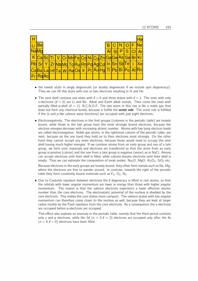
12 ATOMS 193
H He
Li Be
Sc
Mg
Ti
Na
V
CB ON F Ne
Ar
Rn
Kr
Xe
ClSPSiAl
Ca
Cs
Fr
K
Rb
Ba
Ra
Ge
Sn
Tl
Ga
Pb
In
Se
PoBi
Sb
As
Te
At
I
Br
Hg
Cd
Zn
Au
Ag
CuCr MnFe Co Ni
Y ZrSr Mo
TaHf
Ac
La
Nb Tc
ReW Os Ir Pt
Ru PdRh
• the lowest state in singly degenerate (or doubly degenerate if we include spin degeneracy).Thus we can fill this state with one or two electrons resulting in H and He.
• The next shell contains one state with ` = 0 and three states with ` = 1. The ones with onlys-electrons (` = 0) are Li and Be. Alkali and Earth alkali metals. Then come the ones withpartially filled p-shell (` = 1), B,C,N,O,F. The last atom in this row is Ne a noble gas thatdoes not form any chemical bonds, because it fulfills the octet rule. The octet rule is fulfilledif the (s and p like valence wave functions) are occupied with just eight electrons.
• Electronegativity: The electrons in the first groups (columns in the periodic table) are looselybound, while those in the last group have the most strongly bound electrons, because theelectron energies decrease with increasing atomic number. Atoms with low lying electron levelsare called electronegative. Noble gas atoms, in the rightmost column of the periodic table, areinert, because on the one hand they hold on to their electrons most strongly. On the otherhand they cannot accept any more electrons, because those would need to occupy the nextshell having much higher energies. If we combine atoms from an early group and one of a lategroup, we form ionic materials and electrons are transferred so that the atom from an earlygroup is positive (cation) and the one from a late group is negative (anion) as in NaCl. Anionscan accept electrons until their shell is filled, while cations donate electrons until their shell isempty. Thus we can estimate the composition of most oxides: Na2O, MgO, Al2O3, SiO2 etc.
Because electrons in the early groups are loosely bound, they often form metals such as Na, Mg,where the electrons are free to wander around. In contrast, towards the right of the periodictable they form covalently bound materials such as F2, O2, N2.
• Due to Coulomb repulsion between electrons the ` degeneracy is lifted in real atoms, so thatthe orbitals with lower angular momentum are lower in energy than those with higher angularmomentum. The reason is that the valence electrons experience a lower effective atomicnumber than the core electrons. The electrostatic potential of the nucleus is shielded by thecore electrons. This makes the core states more compact. The valence states with low angularmomentum can therefore come closer to the nucleus as well, because they are kept at largerradius mostly by the Pauli repulsion from the core electrons. As a consequence the s-electronsare occupied before p-electrons are occupied.
This effect also explains an anomaly in the periodic table, namely that the third period containsonly s and p electrons, while the 3d (n = 3, ` = 2) electrons are occupied only after the 4s(n = 4, ` = 0) electrons have been filled.

194 12 ATOMS

Chapter 13
Approximation techniques
In most cases quantum mechanical problems cannot be solved exactly. Therefore, for real-worldproblems, we usually need to resort to approximations or numerical methods, or a combination ofboth. There is no limit to the number of approximation techniques one can use for certain problems.However, there is a set of techniques, that already get us a long way, and the ideas behind theseapproaches can be used to use new approximations for a particular problem.
13.1 Perturbation theory
Perturbation theory can be used to determine the properties of a complex system if a similar systemthat is much simpler can explicitly be solved. For example the complex system may have an approxi-mate symmetry. We can solve the system that has the symmetry exactly fulfilled, which is simpler,and then work out the differences of the real system to our model system.
Perturbation theory is not only an approximation method but in many cases it provides informationmore directly than a brute force approach. This is the case when we are interested in the linearresponse of a quantity to a perturbation. For example we would like the splitting of energy levels ofan atom in an external field, because the splitting may experimentally be accessible. There is notpoint to evaluate all the energy values, when it is possible to calculate the splitting directly.
The first order perturbation is also what is needed in linear response theory. For example wewould like to evaluate the dielectric constant of a gas. The dielectric constant is related to the linearresponse1 of the polarization ~P to an electric field. This response is called the electric susceptibility.
Let us consider a system that can be described by an unperturbed Hamiltonian H0 and a smallperturbation W .2 We assume that we can solve the Schrödinger equation for the unperturbedsystem, and we want to use that knowledge to obtain an estimate for the perturbed system. Thefull Hamiltonian H is given as
H = H0 + W
If the perturbation is small, we need not solve the entire problem, but we can instead use pertur-bation theory. The basic idea of the procedure is as follows: We introduce a scale parameter λ forthe perturbation so that
H(λ) = H0 + λW
1The electric susceptibility is defined by χi ,j = 1ε0
dPidEj
, where ~P is the Polarization or electric dipole density and ~E
is the electric field. The relative dielectric constant is related to the electric susceptibility by εr = 1 + χ. (See ΦSX:Elektrodynamik[32].)
2We use the symbol W standing for the German word “Wechselwirkung” for Interaction, because the interactionbetween particles is often treated by perturbation theory.
195
196 13 APPROXIMATION TECHNIQUES
Thus for λ = 0 we obtain the unperturbed system and for λ = 1 the fully perturbed system. For thisscaled system, the energy eigenvalues and the wave functions depend on λ.
13.2 General principle of perturbation theory
Let us now consider that we would like to evaluate a quantity F , which can be the energy, the wavefunction or the density. Since the Hamiltonian depends on the parameter λ, also the quantity F willdepend on λ. Thus one can write down a Taylor expansion for F (λ) as
F (λ) =
∞∑n=0
1
n!
dnF
dλn
∣∣∣∣λ=0
λn
By inserting λ = 1 we obtain the result for the perturbed system.
F (1) =
∞∑n=0
1
n!
dnF
dλn
∣∣∣∣λ=0
The first few derivatives are easy to evaluate, but the evaluation of higher derivatives is in generalcumbersome. If the perturbation is sufficiently small, higher derivatives also do not contribute much.Therefore, the expression for the quantity F in the perturbed system is approximated by
F (1) ≈nmax∑n=0
1
n!
dnF
dλn
∣∣∣∣λ=0
This is the result for F (1) in perturbation theory of order nmax . Typically, nmax is chosen equal toone or two, leading to first-order (F 1st) and second-order (F 2nd) perturbation theory.
F 1st(1) = F (0) +dF
dλ
∣∣∣∣λ=0
F 2nd(1) = F (0) +dF
dλ
∣∣∣∣λ=0
+1
2
d2F
dλ2
∣∣∣∣λ=0
From the λ-derivative of the Schrödinger equation, we obtain expressions for the λ derivative ofthe energy-eigenvalues and the wave functions. Higher derivatives can be obtained recursively. Thenwe use these derivatives to set up a Taylor-series expansion of energies and wave functions in λ. ThisTaylor-series expansion is truncated, usually already after the linear term, and the truncated series isused as approximation for the values at λ = 1.
Our derivation, shown in the following, deviates from those in most text books, in that wefirst determine the exact λ dependent first derivatives and then form higher derivatives from thoseexpressions instead of forming the first and higher derivatives for λ = 0. The reason for this choice istwo-fold. First it is a little simpler to construct the higher derivatives from the first derivative, whichwe need to evaluate anyway, as compared to determining the second derivative from scratch. Moreimportantly, the λ dependent derivatives can be used to obtain the correct result by integration. Thisprocedure is at times used in numerical evaluations of the perturbed energies and eigenstates, and itis also underlies a number of analytical derivations. The latter, however, are not worked out in thistext.
13.3 Time-independent perturbation theory
Here we show the procedure in detail: We consider now the λ-dependent, orthonormal eigenstates|ψ(λ)〉 of the perturbed Hamiltonian H0 + λW . Since the Schrödinger equation[
H0 + λW︸ ︷︷ ︸H(λ)
−En(λ)]|ψn(λ)〉 = 0

13 APPROXIMATION TECHNIQUES 197
must be fulfilled for any value of λ, we can also form its derivative with respect to λ.[H(λ)− En(λ)
]|ψ′n(λ)〉+
[W − E′n(λ)
]|ψn(λ)〉 = 0
Here we use E′n = dEndλ and |ψ′n〉 = d |ψn〉
dλ .Next we multiply from the left with 〈ψm(λ)|, which corresponds to an eigenstate of the perturbed
Hamiltonian.
0 = 〈ψm(λ)|H(λ)− En(λ)|ψ′n(λ)〉+ 〈ψm(λ)|[W − E′n(λ)
]|ψn(λ)〉
= 〈ψm(λ)|Em(λ)︸ ︷︷ ︸〈ψm(λ)|H(λ)
−En(λ)|ψ′n(λ)〉+ 〈ψm(λ)|W − E′n(λ)|ψn(λ)〉 (13.1)
For m = n the first term vanishes, so that Eq. 13.1 yields an expression for E′n:
DERIVATIVE OF THE ENERGY EIGENVALUE WITH RESPECT TO THE STRENGTH OF THEPERTURBATION
E′n(λ)def=dEndλ
= 〈ψn(λ)|W |ψn(λ)〉 (13.2)
Thus the changes of the eigenvalues are obtained from the expectation value of the perturbation op-erator alone.
Let us now consider Eq. 13.1 with m 6= n.
〈ψm(λ)|Em(λ)− En(λ)|ψ′n(λ)〉+ 〈ψm(λ)|W − E′n(λ)|ψn(λ)〉 = 0
⇒ 〈ψm(λ)|ψ′n(λ)〉 =〈ψm|W |ψn(λ)〉En(λ)− Em(λ)
(13.3)
so that we can express the perturbation of the wave functions as
|ψ′n(λ)〉 =∑m
|ψm(λ)〉〈ψm(λ)|︸ ︷︷ ︸1
|ψ′n(λ)〉
Eq. 13.3= |ψn(λ)〉〈ψn(λ)|ψ′n(λ)〉+
∑m(m 6=n)
|ψm(λ)〉〈ψm(λ)|W |ψn(λ)〉En(λ)− Em(λ)
This solution is, however, not yet unique, because it still depends on the unknown matrix element〈ψn|ψ′n〉. We will show in the following that (1) the real part of 〈ψn|ψ′n〉 vanishes, and (2) that itsimaginary part can be chosen equal to zero.
1. We can use the condition that the wave function is normalized for every value of λ:
0 =d
dλ〈ψn(λ)|ψn(λ)〉︸ ︷︷ ︸
=1
= 〈ψ′n(λ)|ψn(λ)〉+ 〈ψn(λ)|ψ′n(λ)〉 = 2Re〈ψn(λ)|ψ′n(λ)〉
Thus the real part of 〈ψ′n|ψn〉 vanishes.
2. What about the imaginary part? It is arbitrary! This is shown as follows: Consider a λ-dependent wave function |ψn(λ)〉. For each value of λ the wave function can be multipliedwith a phase factor eiφ(λ). The resulting wave function
|ψn(λ)〉 = |ψn(λ)〉eiφ(λ)

198 13 APPROXIMATION TECHNIQUES
is an eigenstate for each strength of the perturbation if the same is true for |ψn(λ)〉. Now weform the derivative
|ψ′n(λ)〉 =d
dλ
(|ψn(λ)〉eiφ(λ)
)= |ψ′n〉eiφ(λ) + |ψn〉iφ′(λ)eiφ(λ)
⇒ 〈ψn(λ)|ψ′n(λ)〉 = e−iφ(λ)〈ψn(λ)|(|ψ′n(λ)〉+ |ψn(λ)〉iφ′(λ)
)eiφ(λ)
= 〈ψn|ψ′n〉+ 〈ψn|ψn〉︸ ︷︷ ︸=1
iφ′(λ) = 〈ψn|ψ′n〉+ iφ′(λ)
Thus, simply by changing the λ-dependent phase factor φ(λ), the imaginary part of 〈ψn|ψ′n〉can be changed into an any value. All these solutions are equally valid. Therefore, we choosethe most convenient result by setting the imaginary part of 〈ψn|ψ′n〉 to zero. In the followingwe drop the tilde on the wave function.
With the argument just provided, the matrix element 〈ψn|ψ′n〉 vanishes. Thus, with the appropriatechoice of the phase factor, we obtain the final result:
DERIVATIVE OF THE WAVE FUNCTION WITH RESPECT TO THE STRENGTH OF THEPERTURBATION
|ψ ′n(λ)〉 def=d |ψn(λ)〉dλ
=∑
m(m 6=n))
|ψm(λ)〉〈ψm(λ)|W |ψn(λ)〉En(λ)− Em(λ)
(13.4)
Note that Eqs. 13.2 and 13.4 are exact.
13.3.1 Degenerate case
Eq. 13.4 becomes problematic if En is degenerate, because, in this case, terms with a divide-by-zeroappear in the expression for the wave function.
Without limitation of generality, we assume that the degeneracy is present at λ = 0. This is alsothe most relevant case.
The remedy is the following recipe:
1. Determine all the states |Ψn(0)〉 within one multiplet, that is n ∈ M where M is the set ofindices of the states in the same multiplet. A multiplet is the set of degenerate states, that isEn(0) = Em(0) for all n,m ∈ M.
2. determine the matrix elements of the perturbation with the states in the multiplet
Wm,n = 〈ψm(0)|W |ψn(0)〉 with n,m ∈ M
and diagonalize it so that
W~cj = ~cjwj or∑m
Wn,mcm,j = cn,jwj
The eigenvalues are wj and the eigenvectors are ~cj .
3. Form a new basisset so that
|ψj(0)〉 =∑m
|ψm(0)〉cm,j
13 APPROXIMATION TECHNIQUES 199
4. Now we set up the equation Eq. 13.1 that we obtained before,with the difference that we usethe new states with a tilde.
〈ψm|ψ′n〉(εm − εn) + 〈ψm|W |ψn〉 − 〈ψm|ψn〉ε′n = 0
• Case 1: εm = εn
〈ψm|W |ψn〉 − 〈ψm|ψn〉ε′n = 0
⇒ wnδm,n − ε′nδm,n = 0
⇒ ε′n = wn
• Case 2:
|ψ′n〉 =∑m∈M|ψm〉〈ψm|ψ′n〉+
∑m/∈M
|ψm〉〈ψm|W |ψn〉εn − εm
Next we need to show that the matrix elements 〈ψm|ψ′n〉 can be chosen equal to zero.This is shown as follows: we begin with the λ-derivative of the normalization condition
〈ψm|ψn〉 = δm,n∂λ⇒ 〈ψ′m|ψn〉+ 〈ψm|ψ′n〉 = 0
⇒ 〈ψ′m|ψn〉 = −〈ψ′n|ψm〉
This shows that the matrix 〈ψm|ψ′n〉 is anti-hermitian. In the following we proceed anal-ogously to what has been done before by adding a lambda-dependent phase factor. Here,however we need to generalize the argument to several states.We consider a unitary transformation U(λ) = eA(λ) of the states in the multiplet,
| ¯ψn(λ)〉 =∑m
|ψm(λ)〉Um,n(λ) =∑m
|ψm(λ)〉(
eA(λ))m,n
where A(λ) is a antihermitian matrix, that is A† = −A.It can be shown as follows, that U := eA is unitary, if A is antihermitian:
U†U =(
eA)†
eA = eA†eA = e−AeA = 111
We require that the transformation is the identity for λ = 0, that is U(λ = 0) = 111 orA(λ = 0) = 000.Now we evaluate our expression
| ¯ψ′n(λ)〉 = |ψ′m(λ)〉(
eA(λ))m,n
+ |ψm(λ)〉(AeA(λ)
)m,n
U(λ=0)=111⇒ | ¯ψ′n(0)〉 = |ψ′m(λ)〉+ |ψm(λ)〉(A′′′)m,n
〈 ¯ψm(0)| ¯ψ′n(0)〉 = 〈ψm(0)|ψ′n(0)〉+∑k
〈ψm(λ)|ψk(λ)〉︸ ︷︷ ︸δm,k
A′k,n
λ=0= 〈ψm(λ)|ψ′n(λ)〉+ A′m,n
Thus one can always find a λ-dependent, unitary transformation so that the states withinthe multiplet do not contribute to the derivative.
Thus, for the degenerate result we obtain

200 13 APPROXIMATION TECHNIQUES
DERIVATIVES OF ENERGIES AND WAVE FUNCTIONS IN THE DEGENERATE CASE
ε′n(λ) = 〈ψn(λ)|W |ψn(λ)〉
|ψ′n(λ)〉 =∑
m(εm(λ) 6=εn(λ))
|ψm(λ)〉〈ψm(λ)|W |ψn(λ)〉εn(λ)− εm(λ)
where
〈ψn(λ)|W |ψm(λ)〉 = wnδm,n
for all states in the same multiplet.
13.3.2 First order perturbation theory
Now we use the derivatives Eq. 13.2 and Eq. 13.4 for the unperturbed system, and express theperturbed values as Taylor series.
En(λ) =∑j
1
j!
d jEndλj
∣∣∣∣λ=0
λj
This Taylor expansion is evaluated for the full perturbation that is for λ = 1.
⇒ En(λ = 1) =∑j
1
j!
d jEndλj
∣∣∣∣λ=0
Then we do the actual perturbations by truncating the expansion after the n-th-order term in λ forthe n-th order perturbation theory. In practice only the first and second order perturbation theory isused frequently. For the first order perturbation theory we calculate
E1st ordern ≈ En(λ = 0) +
dEndλ
∣∣∣∣λ=0
and for the second order perturbation theory we include also the next term
E2nd ordern ≈ En(λ = 0) +
dEndλ
∣∣∣∣λ=0
+1
2
d2Endλ2
∣∣∣∣λ=0
For the wave function we proceed completely analogously.
FIRST ORDER PERTURBATION THEORY
The energy En(1) and the energy eigenstates |ψn(1)〉 for a perturbed Hamiltonian H(1) = H0 + Whave the form
En(1) = En(0) + 〈ψn(0)|W |ψn(0)〉+O(W 2)
|ψn(1)〉 = |ψn(0)〉+∑
m(εm 6=εn)
|ψm(0)〉〈ψm(0)|W |ψn(0)〉En(0)− Em(0)
+O(W 2)
where En(0) are the energy eigenvalues and |ψn(0)〉 are the eigenstates of the unperturbed Hamilto-nian H0
Note, that special precaution is necessary for degenerate states!
13 APPROXIMATION TECHNIQUES 201
Linear response
Once we have an approximation for the wave function in a certain order, we can evaluate the pertur-bation not only of the energy but of any other observable up to this order. Note, that some terms,which turn up during squaring the wave functions, need to be dropped. We illustrate the principle onthe first-order result
〈ψn(λ)|A|ψn(λ)〉 =(〈ψn(0)|+ λ〈ψ′n(0)|
)A(|ψn(0)〉+ |ψ′n(0)〉λ
)+O(λ2)
= 〈ψn(0)|A|ψn(0)〉+ λ(〈ψn(0)|A|ψ′n(0)〉+ 〈ψ′n(0)|A|ψn(0)〉
)+λ2
(λ〈ψ′n(0)|A|ψ′n(0)〉
)+O(λ2)
= 〈ψn(0)|A|ψn(0)〉
+λ(〈ψn(0)|A|ψ′n(0)〉+ 〈ψ′n(0)|A|ψn(0)〉
)+O(λ2)
Thus we obtain
〈ψn(1)|A|ψn(1)〉1st order≈ 〈ψn(0)|A|ψn(0)〉+ 〈ψn(0)|A|ψ′n(0)〉+ 〈ψ′n(0)|A|ψn(0)〉
LINEAR RESPONSE
Thus the linear response δAn of an expectation value An of an observable A in an eigenstate |ψn〉 ofthe Hamiltonian due to a perturbation W is obtained by the following expression.
δAndef= 〈ψn(1)|A|ψn(1)〉 − 〈ψn(0)|A|ψn(0)〉 = 2Re
∑m(m 6=n)
〈ψn|A|ψm〉〈ψm|W |ψn〉En − Em
To give an example, this expression may be useful to determine the dipole of a molecular moleculethat is induced by an external electrical field. The proportionality constant is the polarization of themolecule.
13.3.3 Second order perturbation theory
The second-order result for the energy eigenvalues is sufficiently simple so that we show it here. Forhigher order terms even perturbation theory becomes increasingly difficult so that it is rarely done.
The second derivatives of En(λ) and |ψn(λ)〉 are obtained from Eq. 13.2 and Eq. 13.4, whichare valid for any value of λ, by deriving them once more with respect to λ. The resulting expressioncontains first derivatives that are known already. Finally, we insert the result into the Taylor expansionup to second order about λ = 0 and set λ = 1
E′n = 〈ψn|W |ψn〉
E′′n = 〈ψ′n|W |ψn〉+ 〈ψn|W |ψ′n〉Eq. 13.4
= 2∑m( 6=n)
|〈ψm|W |ψn〉|2
En − Em
En = En + E′n +1
2E′′n
= En + 〈ψn|W |ψn〉+∑m( 6=n)
|〈ψm|W |ψn〉|2
En − Em
Note that the sum extends over all states |ψm〉 except |ψn〉. (The index n is fixed.)

202 13 APPROXIMATION TECHNIQUES
En
En
Em
"
Fig. 13.1: Second order correction E′′n by a second level Em. The result of the second order correctionis a “level repulsion”. It is evident that the correction diverges for En = Em indicating the breakdownof the perturbation series for degenerate energy levels.
It may be interesting to consider the effect of the second order correction of the energy levels.The contribution of nearby energy levels is largest, given that the matrix elements are roughly ofsimilar size.
13.4 Time-dependent perturbation theory
The prototypical application of time-dependent perturbation theory is the determination of opticalabsorption spectra. The light-wave creates an oscillating electric field at the site of the transition,and will induce transitions of electrons from an occupied orbital into an un-occupied orbital. Typically,the electric field is sufficiently small to be treated as a small perturbation. The wave length is usuallysufficiently large that we only need to consider a fluctuating, but spatially constant electric field atthe point of the transition. For monochromatic light, the perturbation of the Hamiltonian due to thelight has the following form
W (t) = −~rq ~E0 sin(ωt)
where q is the charge of the excited electron, ~E0 the amplitude of the electric field in the light wave,and ~ω the photon energy.
E1
E2
hω
E1
E2
hω
hω
hω
E1
E2
hω
Fig. 13.2: Sketch of time dependent processes. Left optical absorption: A photon is absorbed andan electron is lifted to a higher energy level. Right: Stimulated emission: If the higher energy levelis occupied and the lower level is filled, a photon can trigger the desorption of another one, whilethe electron drops into the lower energy level. Stimulated emission underlies the workings of a laser.Middle: Spontaneous emission: An electron can drop into the lower level while emitting a photon.This process is similar to stimulated emission, but the photon that triggers the emission is a virtualphoton, i.e. a vacuum fluctuation of the electromagnetic field.

13 APPROXIMATION TECHNIQUES 203
In the following we do not specialize on monochromatic light, but treat a general time-dependentperturbation W (t) of the unperturbed and time-independent Hamiltonian H0.
i~∂t |ψ〉 =(H0 + W (t)
)|ψ〉 (13.5)
We assume that we know the eigenstates of H0
H0|φn〉 = |φn〉En (13.6)
Then we make the Ansatz
|ψ(t)〉 =∑n
|φn〉e−i~Entan(t) (13.7)
and insert it into the time-dependent Schrödinger equation Eq. 13.5. Furthermore, we multiply theequation from the left with 〈φm|,
〈φm|i~∂t |ψ(t)〉 Eq. 13.5= 〈φm|H0 + W (t)|ψ(t)〉
Eq. 13.7⇒∑n
〈φm|φn〉e−i~Ent
(Enan(t) + i~∂tan(t)
)=
∑n
〈φm|H0 + W (t)|φn〉e−i~Entan(t)
Eq. 13.6⇒∑n
〈φm|φn〉︸ ︷︷ ︸δm,n
e−i~Ent
(i~∂tan(t)
)=
∑n
〈φm|W (t)|φn〉e−i~Entan(t)
⇒ e−i~Emt i~∂tam(t) =
∑n
〈φm|W (t)|φn〉e−i~Entan(t)
Division by the phase factor e−iEmt/~ yields
i~∂tam(t) =∑n
〈φm|W (t)|φn〉e−i~ (En−Em)tan(t) (13.8)
This equation is equivalent to the Schrödinger equation Eq. 13.5.Now, we convert the differential equation Eq. 13.8 into an integral equation.
am(t) = am(t0)−i
~∑n
∫ t
t0
dt ′ 〈φm|W (t ′)|φn〉e−i~ (En−Em)t ′an(t ′) (13.9)
Sofar we have not done any approximation. We simply changed to the interaction picture discussedearlier in Section 8.5.3.
Just as in the time-independent perturbation theory, we introduce a scale factor for the pertur-bation W .
H(λ) = H0 + λW
So that H(λ = 1) = H0 + W is the full Hamiltonian and H(λ = 0) = H0 is the unperturbedHamiltonian. Secondly we introduce the truncated Taylor expansions bn,k(λ, t) for the coefficientsan(λ, t), which now not only have a time dependence but also a λ dependence.
bn,k(λ, t)def=
k∑j=0
1
j!
d jan(t)
dλj
∣∣∣∣λ=0
λj (13.10)
The truncated Taylor expansions will converge to the correct result3, if k approaches infinity, that is
limk→∞
bn,k(λ, t) = an(λ, t) (13.11)
3We assume that λ = 1 lies within the convergence radius of the Taylor expansion.

204 13 APPROXIMATION TECHNIQUES
The initial condition is chosen independent of λ.
bn,k(λ, 0) = an(λ, 0) = an(λ = 0, 0) (13.12)
Now we divide4 the above equation Eq. 13.8 into orders of λ and drop all terms with a power ofλ higher than λp
am(λ, t) = am(λ = 0, 0)−i
~∑n
∫ t
0
dt ′〈φm|λW (t ′)|φn〉e−i~ (En−Em)t ′an(λ, t)
⇒ bm,p(t) = am(0)−i
~∑n
∫ t
0
dt ′〈φm|W (t ′)|φn〉e−i~ (En−Em)t ′λbn,p−1(t)
Thus we obtain a recursive relation for increasingly improved estimates bn,p(t) for the coefficients,where the first term is simply bn,0 = an(0). The first two terms have the form
bm,1(t) = am(0)−i
~∑n
∫ t
0
dt ′〈φm|W (t ′)|φn〉e−i~ (En−Em)t ′an(0) (13.13)
bm,2(t) = am(0)−i
~∑n
∫ t
0
dt ′〈φm|W (t ′)|φn〉e−i~ (En−Em)t ′an(0)
−1
~2
∑n,k
∫ t
0
dt ′∫ t ′
0
dt ′′〈φm|W (t ′)|φk〉〈φk |W (t ′′)|φn〉
· e−i~ (Ek−Em)t ′e−
i~ (En−Ek )t ′′an(0) (13.14)
The first approximation bm,1 is the result from first-order perturbation theory, and bm,2 is the resultfrom second-order perturbation theory. Notice, that the highest power of W in the result is equal tothe order of the interaction.
13.4.1 Transition probabilities
Here, we use the expression from first-order perturbation theory to determine the excitation probabilityof a system, such as an optical excitation due to a light pulse. The description here differs fromthat in many text books: Instead of investigating the increase of the excited state probability withtime for a constant beam of light, we use here the excitation probability for a light pulse with a finiteduration. This derivation avoids some of the conceptual problems of other derivations and it is closerto a real experiment.
A more fundamental and explicit derivation for the transition probabilities can be found in ap-pendix I on p. 285.
4If there is an equation of the form
F (t, λ) = G(t, λ)
which is fulfilled for all values of λ, we can form the derivatives.
∂nF (t, λ)
∂λn=∂nG(t, λ)
∂λn
Since all the derivatives of left and right-hand side are equal, also every term of the Taylor expansion
1
n!
∂nF (t, λ)
∂λn=
1
n!
∂nG(t, λ)
∂λn
and the truncated Taylor expansions must be equal.
k∑n=0
1
n!
∂nF (t, λ)
∂λnλk =
k∑n=0
1
n!
∂nG(t, λ)
∂λnλk
This is a fundamental step done in perturbation theory.

13 APPROXIMATION TECHNIQUES 205
We consider a situation where the system is in a specific initial state with quantum number n. Inthe interaction picture, the system at t = −∞ has the wave function amplitudes a(i)
m = δm,n. A lightpulse perturbes the system so that the wave function amplitudes change with time as long as the pulseacts on the system. After the pulse has passed, the wave function amplitudes remain constant5, buttheir values differ from those of the initial state. We denote the final values as a(f )
m = am(t = +∞).In the final state, the system resides with probability Γm,n = |a(f )
m |2 in state m. Thus we may expressΓm,n as the transition probability from state n to state m.
We begin with the first-order expression Eq. 13.13 for the time-dependent perturbation theory.
am(t)Eq. 13.13
= am(−∞)−i
~∑n
∫ t
−∞dt ′〈φm|W (t ′)|φn〉e−
i~ (En−Em)t ′an(−∞) +O(W 2) .(13.15)
Let us insert a pulse with a given temporal shape and a finite duration,
W (t) = W0eiωtχ(t) , (13.16)
where χ(t) is the pulse shape.The Fourier transform of the pulse shape is obtained from
χ(t) =
∫dω χ(ω)eiωt (13.17)
χ(ω) =1
2π
∫ ∞−∞
dt χ(t)e−iωt (13.18)
A general property of a Fourier transform is that a short pulse automatically leads to a poorfrequency resolution. A monochromatic pulse is necessarily of infinite duration.
If the initial state is am(−∞) = a(i)m , the probability amplitude a(f )
m = am(+∞) in the final stateis to first order
a(f )m
Eq. 13.13= a(i)
m −i
~∑n
〈φm|W0|φn〉[∫ ∞−∞
dt ′ χ(t ′)e−i~ (En−Em−~ω)t ′
]︸ ︷︷ ︸
2πχ( 1~ (En−Em−~ω))
a(i)n . (13.19)
The expression in parenthesis is simply the Fourier transform of the pulse shape. With Eq. 13.18 weobtain
a(f )m = a(i)
m −i
~∑n
〈φm|W0|φn〉 2πχ(1
~(En − Em − ~ω))a(i)
n . (13.20)
After the pulse, the probability Γm,n = |afm|2 of finding the system in the excited state |φm〉, giventhat it started out in state |φn〉, that is |a(i)
j |2 = δj,n, is
TRANSITION PROBABILITY
The transition probability from state n to state m induced by perturbation W (t) = W0eiωtχ(t) withthe pulse-shape function χ(t) is
Pm←n =4π2
~2
∣∣〈φn|W0|φm〉∣∣2 ∣∣∣∣χ(1
~(En − Em − ~ω)
)∣∣∣∣2 (13.21)
where χ(ω) is the Fourier transform of the pulse-shape function as defined in Eq. 13.18. Note, thatχ(ω) has the unit of time and χ(t) is unit-less.
Before we continue let me mention two points:5This is a consequence of the interaction picture.

206 13 APPROXIMATION TECHNIQUES
• The transition probabilities obtained from the equation given above to not add up to unity, i.e.∑m Γm,n 6= 1. This is a consequence of ignoring the contribution of the second-order terms,
which contribute to the same order to the transition probability as the first order terms. Ifall second order terms in the transition probability are taken into account, the probability toremain in the inital state is, as expected, Γn,n = 1−
∑m 6=n Γm,n.
• The transition probability discards the relative phases of the wave function amplitudes in differ-ent states. If we only consider the transition probability to evaluate the time dependence, thesephases could lead to constructive and destructive interference between different sequences ofvirtual excitations. This effect is ignored. The physical assumption is that the phases arerandomized between transitions by some unspecified interaction with an environment. If this isthe case every transition is independent of the other ane we obtain a kinetic equation.
A more fundamental and explicit derivation for the transition probabilities is given in the ap-pendix I on p. 285.
13.4.2 Fermi’s golden rule
Let us now investigate excitations with a long, and nearly feature-less, pulse shape. This implies thatthe frequency spread of the envelope function is neglegible. This will lead us to Fermi’s golden rule,in which the shape of the pulse does no more show up.
This is the common case of an optical excitation. Except for a laser pulse, light consists ofmany waves with specific durations. The duration of a wave pulse is related to a coherence time.Each pulse has a tiny probability for being absorbed, leading to a transition between two levels. Thequestion is to calculate the transition probability per unit time for light made of pulses that add upto a specified intensity.
We will investigate a pulse that is very long and has a good frequency resolution. In this limit,the result becomes independent of the pulse shape.
Norm in the time and in the frequency domain
First, let us translate the norm of the pulse shape in the time-domain into a requirement for thefrequency domain.∫ ∞
−∞dt χ∗(t)χ(t) =
∫dω
∫dω′ χ∗(ω′)χ(ω)
∫ ∞−∞
dt ei(ω−ω′)t
= limT→∞
∫dω
∫dω′ χ∗(ω′)χ(ω)
ei(ω−ω′)T − e−i(ω−ω
′)T
i(ω − ω′)
=
∫dω
∫dω′ χ∗(ω′)χ(ω)2 lim
T→∞
sin((ω − ω′)T )
(ω − ω′)Eq. 13.23
=
∫dω
∫dω′ χ∗(ω′)χ(ω)2πδ(ω − ω′) (13.22)
where we used6
limT→∞
sin(xT )
x= πδ(x) . (13.23)
6The delta function is defined by the result∫dx δ(x)f (x) = f (0) of integrals with “reasonably well-behaved
functions” f (x). With the help of the identity7∫∞−∞ dx
sin(ax)x
= π, we find a direct relation to the delta function∫ ∞−∞
dx f (x) limT→∞
sin(xT )
x=
∫ ∞−∞
dysin(y)
ylimT→∞
f (y
T) =
∫ ∞−∞
dysin(y)
y︸ ︷︷ ︸π
f (0) ,
which establishes Eq. 13.23.

13 APPROXIMATION TECHNIQUES 207
Eq. 13.22 yields ∫ ∞−∞dt χ∗(t)χ(t) = 2π
∫dω |χ(ω)|2 .
saying that the normalization in the time domain results in a normalization of the shape function inthe frequency domain.
Long, monochomatic pulses
To form the limit of nearly monochromatic light pulses, let us imagine a sequence of envelopefunctions such as
χλ(t) =√λχ1(λt) (13.24)
for λ→ 0. All these function have the same norm
τdef=
∫ ∞−∞
dt χλ(t)χ∗λ(t) (13.25)
but which become increasingly more extended. Thus, the frequency spread of the Fourier transform
χλ(ω) =1√λχ1
(1
λω
)(13.26)
becomes infinitesimally small, but, due to Eq. 13.24, the integral remains the same, namely τ .A sequence of functions with this property converges, up to a factor, to the delta function. Thus,
the square of the pulse shape is related to a delta function in the limit of a monochromatic lightpulse.
|χλ(ω)|2 λ→0−→1
2πδ(ω − ω0)
∫dt |χ1(t)|2 (13.27)
When we insert this result Eq. 13.27 into Eq. 13.21, we obtain the special case of monochromaticlight.
Pm←n〈(ω−ω0)2〉→0−→
2π
~2|〈φn|W0|φm〉|2δ
(ω0 −
1
~(εm − εn)
)∫dt |χ(t)|2
=2π
~|〈φn|W0|φm〉|2δ (εm − εn − ~ω0)
∫dt |χ(t)|2 (13.28)
The transition probability due to a monochromatic pulse with shape W (t) = W0eiω0tχ(t) witha smooth pulse shape function χ(t) is
Pm←nEq. 13.28
=2π
~|〈φn|W0|φm〉|2δ (εm − εn − ~ω0)
∫dt |χ(t)|2 (13.29)
This equation says that an excitation with monochromatic light is only possible if the incident lightbeam has exactly that energy ~ω0 that is necessary to lift the system into a higher-, or lower-energeticstate.
Many pulses
This result Eq. 13.31 can be converted into one that gives the transition probability per unit time,rather than the probability for a single pulse. We consider the effect of many light pulses, eachdescribed by its own envelope function χk(t) so that
1
T
∫ T
0
∑k
|χk(t)|2 = 1 (13.30)

208 13 APPROXIMATION TECHNIQUES
A remaining scale factor can be integrated into W0. Then we add up the probabilities from all pulsesand obtain the corresponding transition rate Γm←n. This is Fermi’s golden rule
FERMI’S GOLDEN RULE
The transition rate (transition probability per unit time) due to approximately monochromaticpulses with shape W (t) = W0eiω0tχk(t), having a smooth pulse shape χk(t) and a total intensity1T
∫ T0 dt
∑k |χk(t)|2 = 1 is
Γm→n =1
TPm→n
Eq. 13.31=
2π
~|〈φn|W0|φm〉|2δ (εm − εn − ~ω0) (13.31)
Fermi’s golden rule says that an excitation with monochromatic light is only possible if the incidentlight beam has exactly that energy ~ω0 that is necessary to lift the system into a higher-, or lower-energetic state.
With these transition rates we can investigate the stimulated absorption and stimulated emis-sion of light. The stimulated emission of light underlies the function of a laser. Electrons are preparedin their excited state. They remain there until light stimulates emission, which pumps further en-ergy into the laser beam. Important for the function of a laser is that the spontaneous emission oflight is sufficiently small so that the system can be prepared in its excited state. The latter effectcan be considered as the spontaneous emission of light induced by the zero point vibrations of theelectromagnetic field[4].
13.5 Variational or Rayleigh-Ritz principle
The variational principle is a useful scheme to find the ground state of a system. The ground stateis the energy eigenstate with lowest energy. It is commonly known under the name Rayleigh-Ritzprinciple or Ritz-method.[40]8
Nearly all methods to investigate the electrons in real solids or molecules are based on the varia-tional principle.
The basis for the variational principle is the following observation:
• The energy E[ψ] = 〈ψ|H|ψ〉〈ψ|ψ〉 evaluated for an arbitrary state |ψ〉 is higher than the energy of the
ground state, and
• that it this energy becomes equal to the ground-state energy, if we insert the ground state for|ψ〉
This is very handy if we cannot solve the Schrödinger equation exactly. We just choose an arbitraryfunction, and we can evaluate, if not the ground state energy itself, at least a strict upper bound forit. The better the guess for the wave function the closer we approach the ground state energy.
This is shown as follows:
8Walter Ritz, born 1878 in Sion, Switzerland, died 1909,Goettingen, Germany. swiss theoretical physicist, knownfor the variational principle named after him as well as for the Rydberg-Ritz formula, describing the spectral lines ofthe hydrogen atom. The contribution of Ritz was that the spectral lines can be constructed as differences of energylevels. Walter Ritz died in the young age of only 31 years on tuberculosis.

13 APPROXIMATION TECHNIQUES 209
PROOF: let us expand |ψ〉 =∑
n |φn〉cn with cn = 〈φn|ψ〉 into the orthonormal system of eigenstates |φn〉of the Hamiltonian with eigenvalues En, that is H|φn〉 = |φn〉En and 〈φn|φm〉 = δn,m.
E[ψ]def=〈ψ|H|ψ〉〈ψ|ψ〉 =
〈ψ|H
1︷ ︸︸ ︷∑n
|φn〉〈φn| |ψ〉
〈ψ|∑n
|φn〉〈φn|︸ ︷︷ ︸1
|ψ〉
=
∑n〈ψ
H|φn〉︷ ︸︸ ︷|φn〉En
cn︷ ︸︸ ︷〈φn|ψ〉∑
n〈ψ|φn〉〈φnψ〉=
∑n |cn|
2En∑n |cn|2
E[ψ]− E0 =
∑n |cn|
2(En − E0)∑n |cn|2
≥ 0
Since each term is non-negative the result must be non-negative. The equal sign holds, if all coefficientsvanish except that for the ground state, i.e. for En = E0. Hence the equal sign holds only for the groundstate. q.e.d
The variational principle is the basis for almost all electronic structure methods, that try todetermine the electronic wave functions for real materials. Here we work with N-particle systems,which are often approximated in one or the other way by non-interacting N-particle systems.
Since these systems are often enormously complex, we choose a set of basis functions |χi 〉. Thesefunctions could be atomic orbitals. In this case, the method would be called “linear superposition ofatomic orbitals” (LCAO).9
Then we make an ansatz of these basis functions.
|ψn〉 =∑i
|χi 〉ci ,n
and minimize the total energy for this wave function.If we multiply the Schrödinger equation from the left with a basis function, we obtain a eigenvalue
equation in matrix form
H|ψn〉 = |ψn〉En⇒∑j
〈χi |H|χj〉cj,n =∑j
〈χi |χj〉cj,nEn
⇒ H~cn = O~cnEn
where Hi ,j = 〈χi |H|χj 〉 are the Hamilton matrix elements and Oi ,j = 〈χi |χj〉 are the Overlap matrixelements. If the set of basis functions |χn〉 is complete, this was nothing but a change of therepresentation. No approximation has been done so far.
However, if the basis set is complete, it is also infinite. Such a problem cannot be handled on thecomputer. In practice we thus have to limit the dimension of the vectors and matrices. Only a finiteset of wave functions is used. This however is a fairly uncontrolled approximation. The variationalprinciple provides us with two important conclusions about the approximate solution
• The energy is an upper bound of the ground state energy
• The deviations of the approximate wave functions only induces changes of second order in thetotal energy.
The groundstate of a non-interacting N-Fermion system is a Slater determinant formed by the Neigenstates of the corresponding one-particle Hamiltonian. The energy of this Slater determinant is
9Note that LCAO is not a very good technique for practical electronic structure methods.

210 13 APPROXIMATION TECHNIQUES
given by the sum of the corresponding eigenvalues of the one-particle Hamiltonian. The variationalprinciple shows that every Slater determinant of orthonormal orbitals has an energy larger or equalto the ground state.
E0 ≤ min~c0
F (~c0, λ)
F (~c0, λ) = ~c0H~c0 − λ (~c0O~c0 − 1)
∂F
∂ci ,0=∑j
Hi ,jcj,0 − λO
where λ is a Lagrange multiplier for the constraint ~c0O~c0 = 1, that the wave function is normalized.
PROOF: We describe the trial wave function |ψ〉 =∑
n |φn〉cn as a linear superposition of basis functions |φn〉with variable coefficients cn. Note, that the basis functions need not be complete, orthogonal or normalized.
E[ψ] =〈ψ|H|ψ〉〈ψ|ψ〉 =
∑n,m c
∗n 〈φn|H|φm〉cm∑
n,m c∗n 〈φn|φm〉cm
The minimum condition is dE/dcn = 0 and dE/dc∗n = 0. We have to consider here the coefficient and itscomplex conjugate as independent quantities. There are two derivatives, because each coefficient has a realand an imaginary part. The coordinate transformation from real and imaginary part to a complex coefficientand its complex conjugate is a common trick for handling complex numbers.
dE[ψ]
dc∗k=
d
dc∗k
(∑n,m c
∗n 〈φn|H|φm〉cm∑
n,m c∗n 〈φn|φm〉cm
)=
∑m〈φk |H|φm〉cm∑n,m c
∗n 〈φn|φm〉cm
−∑
n,m c∗n 〈φn|H|φm〉cm∑
n,m c∗n 〈φn|φm〉cm
×∑
m〈φk |φm〉cm∑n,m c
∗n 〈φn|φm〉cm
From the condition that the derivatives vanish, we obtain an equation for the coefficients
⇒ 0 =∑m
〈φk |H|φm〉cm −∑m
〈φk |φm〉cmE
E =
∑n,m c
∗n 〈φn|H|φm〉cm∑
n,m c∗n 〈φn|φm〉cm
What we obtained is a set of nonlinear equations for the coefficients, because E depends itself on thecoefficients. However, the problem can be solved as eigenvalue problem, after identifying E with the lowesteigenvalue. q.e.d
The eigenvalue equation is nothing more than solving the Schrödinger equation in a limited Hilbertspace defined by the basis functions. The more basis functions are included, the lower the energyand the more accurate is the result. By including more and more basis functions we can thereforeapproach the correct solution arbitrarily close.
The variational principle is so powerful, because any deviation in the wave function from theground-state wave function enters only to second order into the energy expression.

13 APPROXIMATION TECHNIQUES 211
PROOF: Here we show that the deviation of the trial wave function from the ground state wave functionenters only to second order in the energy.We expand the trial wave function |ψ〉 into eigenstates |φn〉 of the Hamiltonian with energies En. Thecoefficients of the trial wave function |ψ〉 =
∑n |φn〉cn are written as cn = δn,0 + δcn, where δcn describes the
deviation from the ground state |φ0〉.
E =〈ψ|H|ψ〉〈ψ|ψ〉
=
∑n |δn,0 + δcn|2En∑n |δn,0 + δcn|2
=
∑n(δn,0 + 2Re[δcn]δn,0 + |δcn|2)En∑n(δn,0 + 2Re[δcn]δn,0 + |δcn|2)
=E0(1 + 2Re[δc0]) +
∑n |δcn|
2En
(1 + 2Re[δc0]) +∑
n |δcn|2=E0 +
∑n |δcn |2En
1+2Re[δc0]
1 +∑n |δcn |2
1+2Re[δc0]
= E0 +∑n
En − E0
1 + 2Re[δc0]|δcn|2 +O(δcn)4
= E0 +∑n
(En − E0)|δcn|2 +O(δcn)3
In the last steps we used 11+x
= 1− x +O(x2). Thus we find that E = E0 +O(δc2n ) q.e.d.
A small error in the trial wave function produces an even smaller error in the energy. Hence, avery good estimate of the ground state energy can be obtained with fairly poor trial wave functions.It must be noted however, that the error in other observables is still of first order. One must not bemisguided from a converged total energy, that the wave function itself is already of good quality. (Acommon mistake!)
Proof of the variational principle for non-interacting many-particle systems (Home study)
Let us start with N one particle states |ψn〉, which are orthonormal, that is 〈ψn|ψm〉 = δn,m. Weneed to show that
N∑n=1
〈ψn|H|ψn〉 =
N∑n=1
En
where En are the eigenvalues of the one-particle Hamiltonian. Let |φi 〉 be the exact eigenstates ofthe one-particle Hamiltonian.
N∑n=1
〈ψn|H|ψn〉 =
N∑n=1
〈ψn|H∑j
|φj〉〈φj |︸ ︷︷ ︸1
|ψn〉 =
N∑n=1
∑j
〈ψn
H|φj 〉︷ ︸︸ ︷|φj〉Ej〈φj |ψn〉
=∑j
Ej
〈φj |N∑n=1
|ψn〉〈ψn|︸ ︷︷ ︸=:P
|φj〉
=∑j
Ej〈φj |Pn|φj〉
We have introduced P , the projection operator on the approximate wave functions chosen. We cannow show that
• 0 ≤ 〈φj |P |φj 〉 ≤ 1.

212 13 APPROXIMATION TECHNIQUES
•∑
j〈φj |P |φj〉 = N. This is shown as follows:
∑j
〈φj |P |φj 〉 =∑j
〈φj |N∑n=1
|ψn〉〈ψn|φj〉 =
N∑n=1
〈ψn|∑j
|φj 〉〈φj |︸ ︷︷ ︸=1
|ψn〉
=
N∑n=1
〈ψn|ψn〉︸ ︷︷ ︸=1
= N
Now we can calculate the difference from the groundstate energy as
E[ψ1, . . . , ψN ]−N∑j=1
Ej =
N∑n=1
〈ψn|H|ψn〉 −N∑n=1
En
=
N∑j=1
Ej 〈φj |P − 1|φj〉︸ ︷︷ ︸≤0
+
∞∑j=N+1
Ej 〈φj |P |φj 〉︸ ︷︷ ︸≥0
0≤〈φj |P |φj 〉≤1
≥N∑j=1
EN 〈φj |P − 1|φj〉︸ ︷︷ ︸≤0
+
∞∑j=N+1
EN+1 〈φj |P |φj 〉︸ ︷︷ ︸≥0
= (EN+1 − EN)
∞∑j=N+1
〈φj |P |φj 〉 ≥ 0
13.6 WKB-Approximation
The WKB approximation is useful for quasi-one-dimensional potentials, which have little structure ona length scale of the wave length of the particle considered. It is used for example in semiconductorphysics to investigate the transport of charge carriers.
TheWKB approximation10 named after Wentzel, Kramers and Brillouin[41, 42, 43] is also calledthe quasi-classical approximation.
A very good description of he WKB approximation can be found in the book by Griffiths[5].Apparently, the essential features of the WKB approximation have been known as early as
1912[44]. The WKB method is applicable if the potential is rather smooth, so that is itvaries only little over a wave length of the particle. It is also called quasi-classical approximation,because it is a type of perturbation theory, where the small parameter is Planck’s constant ~. (Recallthat ~ = 0 is the classical limit.)
For a given potential, the wavelength of a particle with a given energy scales with ~. Thus thesmaller ~, the better the condition, that the potential varies slowly over the wavelength of a particle,is fulfilled. Even though the WKB approximation can also be applied in higher dimensions, it mostcommonly applied only in one dimension, where it is particularly simple. (The generalization of theWKB method to higher dimensions is nontrivial.)
The WKB method starts with the following Ansatz for the wave function
ψ(x) = ei~S(x)
⇒ pψ(x) =~i∂xei
S(x)~ = ei
S(x)~
(∂xS
)⇒ p2ψ(x) = [
~i∂x ]2ei
S(x)~ = ei
S(x)~
((∂xS)2 +
~i∂2xS)
10In the Netherlands it is called KWB, in France BWK and in Britain JWKB (for Jeffreys). Kramers was dutch,Brillouin french and Jeffreys was british.

13 APPROXIMATION TECHNIQUES 213
When we insert this result into the one-dimensional Schrödinger equation
Eψ =[−~2
2m∂2x + V (x)
]ψ (13.32)
we obtain
E =1
2m(∂xS)2 + V (x) +
~2mi
(∂2xS) (13.33)
Note that we keep the energy fixed in this case. The typical application is to find an approximationfor a wave function at a given energy irrespective of the boundary conditions.11
Now, we expand S in powers of ~, that is
S = S0(x) + ~S1(x) + . . .
We insert this series into the equation (13.33) and order the terms according to powers of ~.12
0 =1
2m(∂xS0 + ~∂xS1 + . . .)2 + V (x)− E +
~2mi
(∂2S0 + ~∂2S1 + . . .)
=[ 1
2m(∂xS0)2 + V (x)− E
]+[ 1
m(∂xS0)(∂xS1) +
1
2mi∂2xS0
]~ +O(~2) (13.34)
For the lowest order, we obtain an expression for S0
(∂xS0)2
2m+ V (x)− E = 0
This is nothing but the classical energy momentum relation, if we identify S0 with the classical actionand ∂xS0 with the momentum.13
11This differs from the applications of first order perturbation theory, where we wanted to find a better bound state.Thus the boundary conditions have been fixed, but the energy depended on the perturbation.
12Note that this step is analogous to that in first order perturbation theory.13The momentum is indeed the gradient of the action which can be shown as follows. We start with the variation
of the action. However, in contrast to the derivation of the Euler Lagrange equations, we allow also variations of theend points of the trajectory.
S[x(t)] =
∫dt L(x(t),
.x(t), t)
δS = S[x(t) + δx(t)]− S[x(t)] =
∫dt
[∂L∂xδx(t) +
∂L∂.xδ.x(t)
]=
∫dt
[∂L∂xδx(t) +
d
dt
(∂L∂.xδx(t)
)− δx(t)
d
dt
(∂L∂.x
)]=
∫dt δx(t)
[∂L∂xδx(t)−
d
dt
(∂L∂.x
)]︸ ︷︷ ︸
ELG
+
∫dt
d
dt
(∂L∂.xδx(t)
)
If we consider now physical trajectories, which fulfill the Euler-Lagrange equation, the term denoted by “ELG” vanishesand only the last term remains. Noting that the canonical momentum is defined as p = ∂L/∂.x , we obtain
δS =
∫ tf
ti
dtd
dt
∂L∂.x︸︷︷︸p
δx(t)
= p(tf )δx(tf )− p(ti )δx(ti )
If we now consider the variation of the action under a variation of the end point along the trajectory, we obtain
dS
dx(tf )= p(tf )
214 13 APPROXIMATION TECHNIQUES
p(x) = ∂xS0 = ±√
2m(E − V (x)) (13.35)
S0(x) = ±∫ x
dx ′p(x ′) + const. = ±∫ x
dx ′√
2m(E − V (x ′)) + const.
We obtained a closed expression for the lowest term. The corresponding wave function is oscillatory,but with a local wave vector ~k = dS
dx that depends on space.
ψ(x) = Aei~S0(x) + Be−
i~S0(x)
In the classically allowed region, i.e. where V (x) < E, the maxima and minima of the wave functionremain constant in space.
In the classically forbidden region, the momentum is imaginary. p(x) = ±iλ(x) with λ(x) =√2m(V − E). is imaginary. Therefore, also the action is imaginary, so that the wave function
consist out of an exponentially decreasing and an exponentially increasing contribution.Let us now consider the next higher order in Eq. 13.34.
0Eq. 13.34
=1
m(∂xS0)(∂xS1) +
1
2mi∂2xS0
0 = p(x)(∂xS1)−i
2∂xp(x)
∂xS1 =i
2
∂xp(x)
p(x)=i
2∂x ln[|p(x)|] = ∂x i ln[
√|p(x)|]
S1 = i ln[√|p(x)|] + const.
Thus we obtain for as result for the wave function which now includes also an amplitude modulation.
WAVE FUNCTION IN THE WKB APPROXIMATION
ψ(x) =1√|p(x)|
[Ae
i~∫dxp(x) + Be−
i~∫dxp(x)
]where the momentum p(x) is according to Eq. 13.35
p(x) =√
2m(E − V (x))
The WKB approximation always requires the first two terms, S0 and S1, to provide a meaningfulresult. This is because there is a prefactor 1/~ in front of the expansion. Thus, the second term,S1, is required to obtain the wave function to zeroth order in ~.
The zeroth order, however, plays an important historical role, because it captures Bohr’s quan-tization condition, which was one of the first steps towards quantum theory. In that theory, theenergy levels have been quantized by the requirement that only those closed classical trajectoriesare allowed, for which the change of the phase S0(x) along a closed classical path is a multiple ofPlanck’s quantum h = 2π~, that is
∫dxp(x) = ~n. This empirical assumption lead to Bohr’s atom
model, which captured the observed excitation energies between the states of the hydrogen atom.Note that along a closed trajectory S0 must change by 2πn along a closed trajectory in order toavoid a discontinuity in the wave function.
13.6.1 Classical turning points
We can already see that the wave function diverges at classical turning points, that is the pointswhere E = V (x). At those points the series expansion Eq. 13.34 does not converge.
13 APPROXIMATION TECHNIQUES 215
Let us investigate Eq. 13.33 and resolve it for ∂xS
(∂xS) = ±√
2m(E − V (x))−~i
(∂2xS) (13.36)
= ±√
2m(E − V (x))
√1 + i
~(∂2xS)
2m(V − E)(13.37)
The expansion of S in orders of ~ is identical to a Taylor expansion of the last factor. Since theconvergence radius of the Taylor series of
√1 + x is equal to one14 , the expansion converges only if
|∂2xS| <
2m|E − V |~
At the classical turning point with V (x) = E, this condition is violated, unless ∂2xS vanishes to all
orders in ~.Near classical turning points we need to evaluate the Schrödinger equation directly. The problem
can be simplified if the potential is linearized near the turning point. The comparison of asymptoticsolutions of the exact solution and that of the WKB approximation provides connection formulas.We will not go into that detail, but only state the final result. The derivation is given in the appendixApp. K. Here we only list the final result.
MATCHING CONDITION FOR THE WKB SOLUTION AT THE CLASSICAL TURNING POINT
The WKB wave function for a potential with positive slope at the classical turning point can bewritten as
Ψ(x < xcl) =1√|p(x)|
cos(1
~[
∫ xcl
x
dx ′p(x ′)]−π
4)
Ψ(x > xcl) =1√|p(x)|
e−1~∫dx ′p(x ′)
and for negative slope
Ψ(x > xcl) =1√|p(x)|
cos(1
~[
∫ x
xcl
dx ′p(x ′)]−π
4)
Ψ(x < xcl) =1√|p(x)|
e1~∫dx ′p(x ′)
13.7 Numerical integration of one-dimensional problems
The one-dimensional Schrödinger equation can readily be integrated numerically.
[−~2
2m∂2x + V ]ψ = Eψ
We use here a method, that is completely analogous to the Verlet, which has been introduced inΦSX: Klassische Mechanik[14] to numerically solve Newton’s equations of motion. The basic idea isto place the wave function onto a grid xi = ∆i , where ∆ is the grid spacing and i is the integer index
14The convergence radius of a Taylor expansion is at most the distance of the nearest singularity. The square roothas a diverging derivative at the origin, that is for xsing = −1 in
√1 + x . Thus the convergence radius is at most
|xsing | = 1

216 13 APPROXIMATION TECHNIQUES
of the grid point. Now we replace the derivative by the corresponding differential quotients
∂xψ(xi) ≈ψi+1 − ψi−1
2∆
∂2xψ(xi) ≈
ψi+1 − 2ψi + ψi−1
∆2
and obtain the discretized Schrödinger equation15. We resolve it for ψi+1
−~2
2m∆2(ψi+1 − 2ψi + ψi−1) + V ψi = Eψi
ψi+1 = 2ψi − ψi−1 −2m(E − V (xi))∆2
~2ψi
Thus knowing the value of ψ at two successive grid points we can evaluate the wave functionrecursively on all other grid points. With the formula given above we obtain the wave function forincreasing x . If we resolve the discretized Schrödinger equation for ψi−1, we obtain a recursiveequation that leads towards smaller x .
13.7.1 Stability
Numerical solutions are not exact. Two aspects need to be understood. The first is accuracyand the second is stability. Accuracy can be improved by decreasing the grid spacing ∆. Thecomputation becomes more involved so that we have to find a good compromise between accuracyand computational effort. When we try to minimize the computational effort by increasing the gridspacing we run into the problem that the scheme may become unstable, and that it will producequalitatively incorrect results.
Consider for example the classically forbidden region, where we have exponentially increasing andexponentially decreasing solutions. If we integrate downward an exponentially decreasing solution, asmall error will create a small component of the increasing solution, and therefore magnify. Sucha procedure is therefore numerically unstable. If, on the other hand, we integrate in the oppositedirection, and integrate the solution in choosing the direction in which it increases, any error willexponentially die out. Therefore, one is not entirely free in the direction: In the classical forbiddenregion one should always propagate the solution in the direction where the wave function increasesin absolute value.
If one follows an exponentially increasing wave function we need to remember that a computercan only represent numbers up to a maximum value, which is 1.79×10308 for an 8 byte real number.While this is a large number, it can still be reached quickly with an exponential increasing function.It is therefore necessary to check the size of the wave function and rescale the entire solution (onall grid points). A computer is not only limited in representing large numbers, but there is also asmallest number the computer can describe. Where the absolute value of the wave function dropsbelow 2× 10−308, the smallest number on an 8-Byte computer, the wave function will be set exactlyto zero, but there the result can be considered insignificant for most purposes.
15The accuracy of these expressions can be tested by inserting the Taylor expansion of ψ
ψi+1 = ψi + ∆∂xψ +1
2∆2∂2
xψ + +1
6∆3∂3
xψ +1
24∆4∂4
xψ + . . .
ψi−1 = ψi − ∆∂xψ +1
2∆2∂2
xψ +−1
6∆3∂3
xψ +1
24∆4∂4
xψ + . . .
ψi+1 − ψi−1
2∆= ∂xψ +
1
6∆2∂3
xψ +O(∆)4
ψi+1 − 2ψi + ψi−1
∆2= ∂2
xψ +1
12∆2∂4
xψ +O(∆)4
Thus the error introduced is of order ∆2

13 APPROXIMATION TECHNIQUES 217
For an oscillatory solution we need to choose the step size sufficiently small. One should choosethe step size smaller than one percent of the period of the oscillation, that is
∆ <1
10
2π~√2m(E −min[V ])
If the step size is larger than one third of the oscillation period, the algorithm becomes unstable.
13.7.2 Natural boundary conditions
For bound states an important question is how to start up the solution. We cannot use two zerovalues of the wave function because then the result will be the zero state. Here we can use the WKBapproximation. We use the function
ψ(x) = 14√
2m(V (x)−E)e−
1~∫dx√
2m(V (x)−E)
to evaluate the wave function on a grid starting from a point where the WKB approximation issafe. Then we use two such values to follow the solution into the classically allowed region.
We can do this from the left and from the right, but since we do not yet know the correct energy,the solution will not match, where they meet. Here we can use another trick.
We expand the solution in a Taylor series ψ(E) = ψ(E0) + (E − E0) dψdE about one energy. Tofirst order
[−~2
2m∂2x + V − E]
dψ
dE= ψ(E)
We discretize this differential equation to obtain dψdE . To start the solution up, we must of course
also form the energy derivative of the WKB solution. Then we decide on a matching point in theclassically allowed region, and evaluate values and derivatives using the differential quotient.
A prediction of the energy can be obtained from the condition that the logarithmic derivativesmatch
∂xψ+ + dE∂x.ψ+
ψ+ + dE.ψ+
=∂xψ− + dE∂x
.ψ−
ψ− + dE.ψ−
which results in a quadratic equation for dE = E − E0
A+ dEB + CdE2 = 0
A = ψ−∂xψ+ − ψ+∂xψ−
B =.ψ−∂xψ+ −
.ψ+∂xψ− + ψ−∂x
.ψ+ − ψ+∂x
.ψ−
C =.ψ−∂x
.ψ+ −
.ψ+∂x
.ψ−
We first test if there is a solution by checking if B2 − 4AC > 0. If there is no such solution, welinearize the equation and use E = E0 − B/A as the next better estimate for the energy.
If there is such a solution for dE from the quadratic equation, we solve this equation and take thesolution for dE with the smaller absolute value to obtain a new estimate for the energy E = E0 +dE.Using this value, we repeat the procedure until the energy is converged. Now we rescale the solutionsso that their values are identical at the matching points.
13.7.3 Radial wave functions for atoms
The radial Schrödinger equation has the form ψ(~r) = φ`,m(|r |)Y`,m(~r)
0 =[−~2
2m
1
r∂2r r +
~2`(`+ 1)
2mr2+ V (r)− E
]φ`,m(r)
=1
r
[−~2
2m∂2r +~2`(`+ 1)
2mr2+ V (r)− E
]rφ`,m(r)

218 13 APPROXIMATION TECHNIQUES
For an atom the potential has singularities at the origin. Therefore, a uniform step-size will notbe appropriate. We need to choose a step size that becomes finer near the origin. Therefore, weintroduce a logarithmic grid. First we introduce a variable transform
r(x) = eαx
which results in
df
dx=df
dr
dr
dx= αr
df
dr⇒ ∂r =
1
αr∂x
∂2r = −
1
αr2∂x +
1
α2r2∂2x
and obtain, after multiplication from the left with r , the transformed radial Schrödinger equation[ −~2
2mα2r2∂2x −
−~2
2mαr2∂x +
~2`(`+ 1)
2mr2+ V (r)− E
]rφ`,m(r) = 0
⇒[−~2
2m(∂2x − α∂x) +
α2~2`(`+ 1)
2m+ α2r2(V (r)− E)
]rφ`,m(x) = 0
This form has no more divergent terms at the origin. We discretize along x and use standardprocedures. The grid becomes infinitely fine at the origin, so that the divergent terms can be easilyintegrated. At the origin of r that is for x → −∞ we need to obey the correct initial conditions. Wechoose the innermost grid point and use the asymptotic solution at the origin to evaluate the wavefunction at the first two grid points.
13.8 Recommended exercises
1. Optical absorption: Exercise 16.8 on p. 244. (Not ready)
2. Alpha decay: Exercise 16.9 on p. 247. (Not ready)
3. Tunneling barrier. Exercise 16.10 on p. 247. (Not ready)
4. Transmission coefficient. Exercise 16.11 on p. 247. (Not ready)

Chapter 14
Relativistic particles
In the first chapter we have learned that the hanging linear chain describes relativistic particles, andthat the Schrödinger equation is the non-relativistic approximation. While the Schrödinger equation isappropriate to describe most observations, there are instances where relativistic effects are important.For example, close to the nucleus, electrons gain sufficient kinetic energy that their velocity becomescomparable to the speed of light. Therefore, atoms contain relativistic effects from that region.
14.1 A brief review of theory of relativity
We are already familiar with the Klein-Gordon equation which we derived from the linear chain afterintroducing a mass term. After applying the correspondence principle, the Klein-Gordon equationresulted in the relativistic dispersion relation E(p) with E2 = p2c2 + m2
0c4. All relativistic particles
obey the same dispersion relation. This dispersion relation lead Einstein to propose the famousequivalence of energy and mass E = m0c
2, which is at the root of nuclear power, peaceful or deadly.This dispersion relation is symmetric with respect to transformations that leave E2 − p2c2 in-
variant. Energy and momentum are related through the correspondence principle to derivatives ofspace and time. This implies that 1
c2 ∂2t −∇2 is an invariant of the symmetry groups of free space. It
might be interesting to find out what these symmetries are and if we can learn something from thesymmetry of the dispersion relation about the geometric structure of space and time.
The relativistic dispersion relation can be written with the help of the metric tensor1
gi ,j =
−1 0 0 0
0 1 0 0
0 0 1 0
0 0 0 1
and the four-dimensional momentum p = (E/c, px , py , pz) = ~
i (− 1c ∂t ,∇) as
3∑i ,j=0
(pic)g−1i ,j (pjc) +m2
0c4 = 0
We use here the notation that the momentum has a zeroth component, which is related to theenergy by p0 = E/c . The momentum is a four dimensional vector just as time and space are writtenin the formulation of the theory of relativity as four dimensional vector (ct, x, y , z). The components
1There are a number of different notations that are equivalent. Often the element −1 of the metric tensor is writtenas − 1
c2 and often the metric tensor has opposite sign. These are all equivalent notations. I have chosen one where themetric tensor is dimensionless, and where the four-dimensional momentum vector has dimensions mass*length/time
219

220 14 RELATIVISTIC PARTICLES
of the four dimensional momentum vector are the canonical conjugate momenta of the correspondingfour-dimensional coordinate vector. For example the energy is conserved if the equations of motionare translationally invariant in time. The momentum is conserved if they are translational invariantin space.
Let us now consider coordinate transformations that leave 1c2 ∂
2t −∇2 invariant. Let us write the
coordinate transformation as
x ′i =
4∑j=0
∂x ′i∂xj
xj =
4∑j=0
Ri ,jxj
What is the corresponding transformation of derivatives?
∂iψ =
4∑j=0
∂x ′j∂xi
(∂′jψ) =
4∑j=0
(Rj,i∂′j)ψ
We have used here 2 the vector ∂i = ∂∂xi.
In a vector notation we can write
x ′ = Rx
∂ = RT ∂′
The symmetry operations of free space are coordinate transformations R that leave ∂g−1∂ =− 1c2 ∂
2t +∇2 invariant. These operations are called Lorentz transformations What are those trans-
formations?
∂g−1∂ = ∂′Rg−1RT ∂′ = ∂′g−1∂′
Rg−1RT = g−1
This is the defining equation for the symmetry operations.We can show that all those transformations leave a certain distance d =
√c2t2 − r2 in the
four-dimensional space invariant.
x ′gx ′ = xRT gRx = x(gR−1g−1)gRx = xgx
c2t ′2 − r ′2 = c2t2 − r2
The invariance of this length is taken to define the basic symmetry of space. What is the distancebetween two space-time points. Two points that are spatially distant can still have zero distance inspace time, namely when it takes the speed of light to get from (r1, t1) to (r2, t2).
Now we can investigate the symmetry operations in more detail: Let us consider a few examples.Translations in time and space conserve d . Also Rotations conserve the length. The rotation in thex,y-plane can be written as (
x ′
y ′
)=
(cos(φz) sin(φz)
− sin(φz) cos(φz)
)(x
y
)
When we replace x in the four-dimensional distance by x ′, we obtain the same result. Similarly ifa physical path of a particle is x(t) then also x ′(t ′) is a physical path, that obeys the equations ofmotion.
2Here a more detailed derivation:
∂Ψ(x ′1, x′2, x′3, x′4)
∂xi=∑j
∂Ψ(x ′1, x′2, x′3, x′4)
∂x ′j
∂x ′j (x1, x2, x3, x4)
∂xi=∑j
∂Ψ
∂x ′jRj,i =
∑j
RTi,j∂Ψ
∂x ′j

14 RELATIVISTIC PARTICLES 221
There must be also a similar transformation in the ct, x plane that conserves the four-dimensionaldistance (
ct ′
x ′
)=
(cosh( vc ) sinh( vc )
sinh( vc ) cosh( vc )
)(ct
x
)
It can be easily shown using cosh2(x)− sinh2(x) = 1 that the distance c2t2− x2 is conserved. Whatis the physical meaning of this transformation? Let us investigate the nonrelativistic limit, that isc →∞. We obtain the Galileo transformation
x ′ = x − vtt ′ = t
Invariance with respect to this transformation simply means that if a path physical x(t) obeys theequations of motion, also the path x ′(t ′) = x(t) +vt obeys the same equations of motion. This is ofcourse true for the free particle. The transformed path is the original x(t) as it is seen by an observermoving with velocity −v . If the speed of light c is finite, as it is in reality, the transformation of theequations of motion is more complex.
In order to build a relativistic theory, we need only to start combining so-called invariants of thesymmetry group to build up the Lagrangian, from which the equations of motion are derived. Oncewe have such a theory, we might look for particles in the real world that are described by such atheory. This is one way to come up with theories for new particles.
We have already seen that E2 − p2c2 is such an invariant and another is m20c
4. Adding the twoinvariants, we arrive at the relativistic dispersion relation, from which we started. The correspondenceprinciple brings us back to the Klein-Gordon equation, which describes so-called scalar particles.However there are other invariants, for example we might express the wave function as an array ofwave functions in each point. The wave function of such a particle is called a spinor wave function.Now we can build up new invariants from operators acting on the spinor components, which still areLorentz invariant in space-time. One very important vector particle are photons, which are spin-oneparticles. Another are electrons and other particles with spin 1
2 .
14.2 Relativistic Electrons
The Dirac equation can be written as(E −
∑i
αicpi − βm0c2)|Ψ〉 = 0 (14.1)
where the energy is here an operator, namely E = i~∂t and the momentum is the momentum operatorp = ~
i ∇. The factors αi and βi are themselves operators acting not on the spatial variable but in afour-dimensional spinor space. We will come to that later. For now we need to remember that αiand β may not commutate among each other.
One condition for a relativistic wave equation is that it reproduces the relativistic dispersionrelation E2 = p2c2 + m2
0c4. We get there by multiplying the Dirac equation from the left with
E +∑
i αicpi + βm0c2.
(E2 −
3∑i ,j=1
αipic2αjpj −
3∑i=1
m0c3[αiβ + βαi ]pi −m2
0c4β2)|Ψ〉 = 0
The relativistic dispersion operator is obtained when the conditions
1
2[αi , αj ]+ = δi ,j
1
2[αi , β]+ = 0
1
2[β, β]+ = 1

222 14 RELATIVISTIC PARTICLES
These equations cannot be fulfilled when α and β are simple numbers. A solution can be found byassuming that the αi and βi are matrices in a four dimensional space. This statement does not referto the space-time, but to four components of the wave function |Ψ〉.
There is one solution, namely
αi =
(0 σi
σi 0
)β =
(1 0
0 −1
)where the σi ’s are the Pauli matrices and the 1’s are two-by-two unit matrices.
σx =
(0 1
1 0
)σy =
(0 −ii 0
)σz =
(1 0
0 −1
)1 =
(1 0
0 1
)The four spinor components of the wave function |Ψ〉 describe
• an electron with spin up
• an electron with spin down
• a positron with spin up
• a positron with spin down
Thus the Dirac equation, which describes leptons such as electrons, for free particles has theform [
i~∂t111−~ci
3∑j=1
αj∂xi −m0c2β]|Ψ〉 = 0 (14.2)
Note that the wave function |Ψ〉 is four component spinor, and that the matrices 111, αj , and β arematrices acting on this four component spinor.
Positrons[45] are antiparticles of the electron. They have identical mass but opposite charge asthe electron. A positron and an electron can annihilate each other by creating two photons. Thephotons carry the energy of the rest mass away.
14.3 Electron in the electromagnetic field
The electron(positron) is coupled to the electromagnetic field by replacing
E → E − qΦ
~p → ~p − q ~A
where Φ(r) is the electric potential and ~A is the vector potential. They are defined as ~E = −~∇φ−∂t ~Aand ~B = ~∇ × ~A.The charge of the electron is negative, that is q = −e where e is the elementarycharge, which is positive.
Thus the Dirac equation has the form(E − qΦ−
∑i
αic(pi − qAi)− βm0c2)|Ψ〉 = 0 (14.3)
If we split the four-component spinor into two two-component spinors (|φ〉, |χ〉), the Dirac equa-tion has the form (
m0c2 + qΦ− E
∑i σi(pi − qAi)c∑
i σi(pi − qAi)c −m0c2 + qΦ− E
)(|φ〉|χ〉
)= 0 (14.4)
where the first two component spinor |φ〉 is attributed to electronic degrees of freedom for spin-upand spin-down electrons and |χ〉 describes spin-up and spin-down positron.

14 RELATIVISTIC PARTICLES 223
14.4 Down-folding the positron component
The four components of the Dirac spinor can be attributed to electrons with spin up and spin downand positrons with spin up and spin down. The positron is the anti-particle of the electron. While aDirac particle is usually a superposition of electronic and positronic components, in the non-relativisticlimit, the two different components can be decoupled exactly.
In this case, we are interested in describing electrons. Therefore, we consider solution withan energy close to E = +m0c
2. In this case, we can show that the positronic components arefairly small. Therefore, one often names the electronic components |φ〉 the “large components”,while the positronic components |χ〉 are named “small component”. We do not want to ignore thepositronic components, but we can simplify the equations by eliminating the positronic componentsin an effective way.
In order to simplify the following equations let us introduce a quantity
M(ε, r) = m0 +ε− qΦ
2c2
and the energy ε with the rest-energy removed
ε = E −m0c2
Note that M is not the relativistic mass defined as mr = m0
√1 + ( p
m0c)2 = m0 + p2
2m0c2 + O( 1c2 ) =
m0 + ε−Vc2 .
Thus we obtain (qΦ− ε
∑i σi(pi − qAi)c∑
i σi(pi − qAi)c −2Mc2
)(|φ〉|χ〉
)= 0
We can now use the second line of the equation to obtain |χ〉 as function of the electron com-ponents |φ〉,
|χ〉 =1
2Mc
∑i
σi(pi − qAi)|φ〉,
which we then insert in to the first equation to eliminate the explicit dependence on the positrons.(∑i
σi(pi − qAi)1
2M
∑j
σj(pj − qAj) + qΦ− ε)|φ〉 = 0
We can use the equation
(~σ ~A)(~σ ~B) = ~A~B + i~σ(~A× ~B) (14.5)
which connects the vectors ~A and ~B and the vector formed by the Pauli matrices. When we applythis equation to operators one has to take care of the commutation relations.
[∑i
(pi − qAi)1
2M(pi − qAi) + qΦ + i
∑i
σi
(~p − q ~A)×
1
2M(~p − q ~A)
)i− ε]|φ〉 = 0 (14.6)
Note that this equation is still nonlinear in energy and electromagnetic field, via the dependence onthe relativistic mass.
Furthermore the wave function φ is not normalized. The correct normalization is
1 = 〈φ|φ〉+ 〈χ|χ〉 = 〈φ|1 + (~σ~p − q ~A)1
(2Mc)2(~σ~p − q ~A)|φ〉
In the last term the magic Eq. 14.5 has been used.

224 14 RELATIVISTIC PARTICLES
14.5 The non-relativistic limit: Pauli equation
Let us now form the non-relativistic limit by setting c =∞ in Eq. 14.6. In that case the relativistic"mass" M is equal to the rest mass m0, which is constant in space. Thus we obtain the so-calledPauli equation.
PAULI EQUATION
[(~p − q ~A)2
2m0+ qΦ−
q
m0
~S ~B − ε]|φ〉 = 0 (14.7)
We have used here that
(~p − q ~A)× (~p − q ~A) = −q(~p × ~A+ ~A× ~p) = i~q(~∇× ~A+ ~A× ~∇) = i~q ~B
~B = ~∇ × ~A + ~A × ∇ is the magnetic field. Here we have expressed the magnetic field as operatorequation, where ∇ not only acts on ~A but also any function tow which this operator is applied to.The magnetic field obtained this way is a simple vector function of real space.
The spin is written as
~S =~2~σ
where ~σ = (σx , σy , σz) are the Pauli matrices.Equation 14.7 differs from the Schrödinger equation only by the Stern-Gerlach term in the
Hamiltonian3
HSG = −q
m~S ~B(~r)
which describes the energy of a magnetic moment ~m = qm~S in a magnetic field ~B. Because the spin
of an electron has the eigenvalues ± ~2 , the magnetic moment of the electron is µb = ~q2m0
. Thisfundamental constant is called the Bohr magneton. The magnetic moment in the Dirac equation isthe origin of interpreting the spin as the rotation of a particle about its own axis, which is a strangeconcept for a point particle.
For a classical particle rotating about a center, magnetic moment and angular momentum arerelated by the relation ~m = q
2m~L. The ratio between magnetic moment and angular momentum is
called the gyromagnetic moment. For a classical particle the gyromagnetic moment is thereforeγ = q
2m . For other charge distributions the ratio between angular momentum and magnetic momentdiffers, which is taken into account by the g-factor g so that in general ~m = g qm
~L. Comparisonwith the Pauli equation indicates that the g-factor of the electron is ge = 2 and the gyromagneticratio of the electron is γe = ge
q2m = q
m . The magnetic moment of the electron is ge = 2.0023. Thedeviation from the value 2 is explained by quantum electrodynamics.
Consider a classical particle circling about the origin in a constant magnetic field ~B. The vector
3It is disturbing that the Pauli equation is a two-component equation, while the Schrödinger equation only has asingle component. In most cases, one can decouple the two components of the Pauli equation by choosing the magneticfield in the z-direction. In that case there are no additional terms that couple spin-up and spin-down components. Thusone arrives at a description that distinguishes between spin-up and spin-down electrons. Each fulfills a Schrödingerequation, albeit with different potentials.

14 RELATIVISTIC PARTICLES 225
potential for a constant magnetic field can be written as ~A = 12~B × ~r . The energy can be written as
E =1
2m(~p − q ~A)2 =
1
2m(~p −
q
2~B × ~r)2
=p2
2m−
q
2m~p(~B × ~r) +
q2
8m(~B × ~r)2
=p2
2m−
q
2m~B(~r × ~p) +
q2
8m(~B × ~r)2
E(~B) = E0 −q
2m~L~B +O(B2)
Now consider the limit where the orbit of the particle goes to zero, so that we obtain a point particle,and the angular momentum approaches the spin of the electron, that is |L| → ~/2. We obtain tofirst order E(B) = E0 − q~
4m~B, assuming that the magnetic moment is parallel to the magnetic field.
Thus we obtain half the value of that obtained from the Dirac equation. The factor missing is calledthe g-factor, and is considered an anomaly. We can attribute it to the fact that the classical particlein our model becomes itself relativistic as the radius is shrunk to zero.
If the magnetic field is parallel to the z-axis, the spin-up and spin-down components are indepen-dent. Each component is a solution of a Schrödinger equation, with the only difference that spin-upand spin-down components experience different potentials V↑ = qΦ − µBBz and V↑ = qΦ + µBBz .If the electron is free to occupy the state with lowest energy, the spin will align parallel and notantiparallel to the magnetic field.
Just as we have determined the Pauli equation for the electrons from the Dirac equation forenergies near E = +m0c
2 after forming the non-relativistic limit, we can similarly determine a Pauliequation for the positrons, that is the solutions with energies near E = −m0c
2. This is done explicitlyin appendix M.2 on p. 314. There we also show that the motion of a positron corresponds indeed toa particle with the opposite charge of the electron.
14.6 Relativistic corrections
Relativistic effects are quite large near the nucleus, where the kinetic energy of an electron approachesinfinity, and the velocity of the electrons approaches that of light.
Relativistic corrections can be observed macroscopically in every compass. A ferromagnet couldnot produce permanent magnetization direction without spin-orbit coupling. Spin-orbit couplinglinks the magnetization to the crystal geometry. In a compass without spin orbit coupling, themagnetization direction inside the material would orient towards the north-pole, but the needle wouldstay put.
In order to separate out the relativistic effects, let us introduce a new dimension-less variable
D =m
M− 1⇒
1
2M=
1
2m0+
D
2m0
D vanishes in the nonrelativistic limit c →∞, where M = m.By replacing 1
2M by 12m0
+ D2m0
in the two-component Dirac equation Eq. 14.6, and after collectingall terms proportional to D, we obtain the relativistic corrections W to the Pauli equation
W =1
2m0
(~p − q ~A)D(~p − q ~A) + i~σ
((~p − q ~A)D × (~p − q ~A)
)(14.8)
The two component Dirac equation can then be written as (H0 + W − ε)|φ〉 = 0, where H0 is thePauli Hamiltonian and W are the relativistic corrections. Note, that D contains not only a spatialdependence, but also an energy dependence. If we only consider the lowest order of the energydependence, we can remove the explicit energy dependence.
Before we continue, let us investigate some properties of the function D

226 14 RELATIVISTIC PARTICLES
• As mentioned before, D vanishes in the non-relativistic limit.
• close to the relativistic limit that is for sufficiently slow particles, D has the form
D = −ε− V2m0c2
+O(1
c4) = −
p2
4m20c
2+O(
1
c4). (14.9)
where V = qΦ. The function D is negative and measures approximately the ratio of kineticenergy and the rest-energy of the particle.
• Let us consider the spatial dependence of D for an electron near a nucleus: We use V (~r) =qΦ = −Ze2/(4πε0|r |) and ε = 0 as model for the potential in the center of an atom.
D =m0
M− 1 =
1
1 + ε−V2m0c2
− 1 = −(
1 +2m0c
2
ε− V
)−1
≈ −(
1−8πε0m0c
2|r |Ze2
)−1
≈ −1 + 2|~r |rT
+O(r2)
where
rT =Ze2
4πε0m0c2
is the so-called Thomson radius. The Thomson radius gives an indication about the size of theregion near the nucleus, where relativistic effects are important. The Thomson radius lies inthe range of 10−4−10−2 a0, where a0 ≈ 0.529×10⁻¹⁰ m is the Bohr radius. As a comparison,a typical atomic radius is in the range of 3 a0.
Let us now return to the relativistic corrections of Eq. 14.8. To simplify the discussion we willintroduce a number of approximations. As the first simplification we ignore the dependence of therelativistic corrections on the magnetic field. The idea is that usually both, relativistic corrections andthe magnetic field, can be considered as small perturbations, so that they can be treated independentlyto first order.
We obtain
W =1
2m0
~pD~p + i~σ
(~pD × ~p
)(14.10)
The last term in Eq. 14.10 will be identified with the spin-orbit coupling. The first term can bedivided into two terms that will be identified with the Darwin term and the mass-velocity correction.We rewrite ~pD~p in two different ways and average the resulting expressions.
~pD~p = ~p[D, ~p] + ~p2D = −~p[~p,D] + ~p2D = −[~p, [~p,D]]− [~p,D], ~p + ~p2D
~pD~p = [~p,D]~p +D~p2
~pD~p = −1
2([~p, [~p,D]] +
1
2(~p2D +D~p2)
=~2
2(∇2D) +
1
2(~p2D +D~p2)
where (∇2D(~r)) is considered as a function and not an operator. 4 p2 on the other hand is consideredin both cases as an operator. We can rewrite the relativistic corrections as
W =~2
4m0(~∇2D) +
1
4m0(~p2D +D~p2) +
i
2m0~σ(~~pD × ~~p
)(14.11)
= WD +Wmv +WLS (14.12)4Unfortunately the notation of operator equations is not completely consistent. Often, an additional pair of paren-
theses is used to indicate that the operator, in this case ∇2 acts only on the function(s) inside the same pair ofparentheses and not further onto any function in the operator or standing to the right of the operator. The truemeaning must be obtained in the end from the context of the equation. It is always possible, even though in somecases utterly inconvenient to rewrite an operator equation such that every operator acts on everything standing to theright of it.

14 RELATIVISTIC PARTICLES 227
where the first term WD is the Darwin term, Wmv is the mass-velocity correction and WLS is thespin-orbit coupling. We will investigate the three contributions separately.
14.6.1 Spin-Orbit coupling
The last term of the relativistic corrections in Eq. 14.12 is the so-called spin-orbit coupling
WLS =1
2m0i~σ(~pD × ~p
)(14.13)
We will now introduce a some assumptions to allow a physical interpretation.Let us assume that the electrostatic potential is spherically symmetric. As a result, also D is
spherically symmetric, so that we can write
~pD = [~p,D]− +D~p =~i
(∂rD)~r
|r | +D~p
where we consider (∂rD) as a single function. Note again the inconsistency in the notation, becauseone might expect that the radial derivative would need to be applied to any function standing to theright of D as well. Here and in the following we consider (∂rD) as a symbol for a function.
Thus we find
WLS =1
2m0i~σ(~i
(∂rD)
|r | ~r × ~p +D~p × ~p)
=1
2m0i~σ~i
(∂rD)
|r | ~r × ~p
=(∂rD)
m0|r |~L~S
where we used that ~~σ/2 = ~S is the spin operator and ~r × ~p = ~L is the angular momentum operator.The energy splitting resulting from spin-orbit coupling in first order perturbation theory is
∆εLS = 〈ψ|1
m0
(∂rD)
|r |~L~S|ψn〉 = ±
~2`
2m0〈ψ|
(∂rD)
|r | |ψn〉
The spin-orbit coupling splits an atomic energy level with an angular momentum quantum number `into a upper level, where the spin is parallel to the orbital angular momentum, and a lower level withantiparallel spin and orbital momentum. Because the total angular momentum for the parallel spinlevel is j = `+ 1
2 the degeneracy of this upper orbital is 2j + 1 = 2`+ 2. The degeneracy of the lowerlevel is 2`.
For historical reasons one often finds the expression for the spin-orbit coupling in a differentform. Here one employs first the assumption that the relativistic effects are small, that is D =− ε−V
2m0c2 + O( 1c4 ), then one introduces the potential of the hydrogen atom and the assumption that
the energy of the electron is small, that is ε = 0. This yields
∆εLS ≈Ze2~2`
16πε0m20c
2〈ψ|
1
r3|ψ〉
This is a good (or bad) example how one can make incompatible approximations and still get away:Without corrections, D is not singular. However, we now used the approximation of small relativisticeffects, that is relatively slow particles in combination with infinite potential energy, that is fairly fastparticles, which lead us to a divergent expression for D near the nucleus. This is clearly nonsense!What saves the construction, is that (1) the ` = 0 term vanishes, and (2) for other angular momentathe wave functions vanish sufficiently rapid near the nucleus, that they compensate the divergentterm in the integral for the energy splitting.
The spin-orbit splitting is important for the conducting properties of semiconductors with heavierelements such as GaAs. Here the top of the valence band, which has p character is split into 4 bands

228 14 RELATIVISTIC PARTICLES
with spin and orbital angular momentum parallel and two bands, where they are antiparallel. Thespin-orbit splitting of these levels in silicon is 0.044 eV and in the heavier Ge it is already 0.3 eV.
The spin-orbit term is also visible in core level spectroscopy, where the core levels are split due tospin-orbit coupling into two multiplets that are separated by several eV.
14.6.2 Darwin term
In order to make the Darwin term[46]
WD =~2
4m0(~∇2D) (14.14)
more transparent, let us now introduce again our usual approximations. First we keep only the leadingorder in 1
c , so that D = V−ε2m0c2 . Note that this approximation is not valid near the nucleus. I list it
here, because that is what has been done historically. We obtain
WD =~2e(~∇2Φ)
8m20c
2+O(
1
c4)
We can simplify this expression further using the Poisson equation ~∇2Φ = ρε0.
If we specialize our result further to the Coulomb potential of the nucleus V = qΦ = − Ze2
4πε0|r | andε = 0, we obtain
WD ≈~2Z2e2
8ε0m20c
2δ(r)
Thus the Darwin term acts only on s-wave function and shifts those up in energy.
14.6.3 Mass-velocity term
In order to give a physical interpretation to the mass-velocity
Wmv =1
4m0(~p2D +D~p2) (14.15)
from Eq. 14.12, we use
ε− V |ψ〉 ≈~p2
2m0|ψ〉
⇒ 〈ψ|D|ψ〉 ≈ 〈ψ| −~p2
4m20c
2|ψ〉
⇒ 〈ψ|WMV |ψ〉 ≈ 〈ψ| −~p4
8m30c
2|ψ〉
where we use the wave functions of the Pauli equation, implying that we only consider the leadingorder of the correction in 1
c . The classical version of the mass velocity term is the leading term ofthe relativistic energy momentum relation.
ε(p) =
√m2
0c4 + p2c2 −m0c
2 =p2
2m0−
p4
8m30c
2+O(
1
c4)
where we used√
1 + x = 1 + 12x −
18x
2 +O(x3)

Chapter 15
Many Particles
Sofar, quantum theory was actually a theory of classical fields. Just as we describe light by electro-magnetic fields, we introduced fields to describe other particles such as electrons. The new ingredientsare the interpretation of the field amplitude as probability amplitude for particles to occur, and thatwe consequently normalized this probability to one.
15.1 Bosons
Let us return to the continuous linear chain that we investigated in one of the first sections. Weshowed there, that we could form a quantum theory by constructing wave packets that behavelike classical particles. However, since the linear chain itself was build up from particles, we shouldtreat every bead of the chain itself as a quantum particle. This idea is the central idea of secondquantization and the treatment of many particles.
15.1.1 Quantum mechanics as classical wave theory
Let us consider the Lagrangian of the hanging linear chain, which can be also used to describe arelativistic particle. There are several reasons for choosing this model: we can look at it both as aclassical model and a quantum mechanical problem. (1) If we remove the “mass” term that resultsfrom hanging the linear chain, we have a model for a phonon in a crystal. (2) If we ignore thefact that the displacements are real, the displacement field follows the same equations as the Klein-Gordon field, which describes relativistic spin-0 particles, such as mesons. Furthermore we avoid theintricacies of complex field amplitudes in the derivations.
We start out from the Lagrangian Eq. 3.31, which has been derived early in this booklet.
L = K
∫ L
0
dx( 1
c2(∂tφ)2 − (∂xφ)2 −
m20c
2
~2φ(x, t)2
)The first step is to decompose φ(x, t) into eigen modes.1 First we derive the Euler-Lagrange
equations, which are the classical field equations such as the Schrödinger equation. Here we obtain:(−
1
c2∂2t + ∂2
x −m2
0c2
~2
)φ(x, t) = 0
We obtain the time independent equation using the ansatz φ(x, t) = uj(x)e−iωj t(ω2j
c2+ ∂2
x −m2
0c2
~2
)uj(x) = 0
1We could also have staid in the real space formulation, but that would have made the derivation a bit morecomplex. Here I rather choose to transform first into Eigen modes and later transform back into real space.
229

230 15 MANY PARTICLES
The solutions are
uj(x) =1√L
sin(kjx) with kj =2π
Lj
~ωj =
√m2
0c4 + (~kjc)2
where we use periodic boundary conditions φ(x) = φ(x + LL) and the ortho-normalization condition〈uj |uj ′〉 =
∫ L0 dxuj(x)uj ′ = δj,j ′ .
There is one tricky point: We only keep the solution ω > 0 even though the equation has apositive and a negative branch. This is analogous to the harmonic oscillator where the classicalmotion is built from solutions x(t) = Ae+iω0t + Be−iω0t . Nevertheless, we only consider positivefrequency for the harmonic oscillator.
Now we need to introduce the mode decomposition φ(x, t) =∑
j uj(x)φj(t) into the Lagrangian,which we rewrite with the help of Gauss theorem and the Euler-Lagrange equations obtained above.
L = K
∫ L
0
dx( 1
c2(∂tφ)2 + φ(∂2
x −m2
0c2
~2)φ)
= K∑n,n′
( 1
c2(∂tφj)(∂tφ
′j)
∫ L
0
dxuj(x)u′j(x)
+φjφ′j
∫ L
0
dxuj(x)(∂2x −
m20c
2
~2)u′j(x)
)=K
c2
∑j
((∂tφj)
2 − ω2j φ
2j
)In the next step we need to find the Hamilton function for the classical displacement field. We
obtain the the canonical momentum of the displacement field amplitude φj(t),
Πj =∂L
∂.φj
=2K
c2∂tφj ⇒ ∂tφj =
c2
2KΠj
and set up the Hamilton function in the usual way
H(Πj , φj) =∑j
Πj∂tφj − L(φj∂tφj)
=c2
4K
∑j
(Π2j +
4K2ω2j
c4φ2j
)= E
15.1.2 Second quantization
Now we quantize the displacement field φ(x). The procedure is completely analogous to the firstquantization, where we made the transition from a position coordinate x to a wave function φ(x) onthe coordinate space. Here we make the transition from a displacement field or probability amplitudeto a wave function Φ defined on the space spanned by the probability amplitudes. This implies thatthe wave function amplitude φ(x, t) does not have a well defined value but is itself described by awave function Φ[φ(x)]. Note that Φ is a functional of the displacement field. For the linear chain,this is a natural step, because it corresponds to the first quantization of the beads. If however weinterpret φ(x, t) as the probability amplitude of a quantized point particle, things become different.
We use the correspondence principle
E → i~∂t Πj →~i∂φj (15.1)

15 MANY PARTICLES 231
to convert the Hamilton function into a Hamilton operator.We obtain a Schrödinger equation
i~∂t |Φ〉 = H|Φ〉 =c2
4K
∑j
(−~2(∂φj )
2 +4K2ω2
j
c4φ2j
)|Φ〉
where Φ is a wave function that depends on the displacements of all the eigen modes Φ(φ1, φ2, . . .).Note here, that the difference between the Hamilton operator used here and the Hamilton operatorH(p, x) = − ~2
2m∂2x+V (x), that defines the “classical field equations” such as the Schrödinger equation.
Let us try to give some meaning to this Schrödinger equation. What we find is a harmonicoscillator for each vibrational mode. We know how to deal with this from Sec. 5.6. By comparingwith Eq. 5.30, we identify the mass of the harmonic oscillator with m = 2K
c2 and the frequency withω0 = ωj . We introduce the ladder operators a and a† analogous to Eq. 5.33.
aj = i
√c2
4~KωjΠj +
√Kωj~c2
φj
a†j = −i
√c2
4~KωjΠj +
√Kωj~c2
φj
Note that Πj = ~i ∂φj is an operator and no more a classical field with a well defined value at each
position.With the help of εj = ~ωj , the Hamilton operator can be written as
H =∑j
|uj 〉εj(a†j aj +
1
2
)〈uj |
What we get are discrete energy levels with values
E(nj) =∑j
εj(1
2+ nj).
The energy is discretized and comes in bunches, where each quantum carries the energy correspond-ing to the dispersion relation ε(kj) = ~kj . Thus we can interpret each excitations of a vibrationalmode as particle with a wave function with the corresponding eigen mode of the hanging linear chain.We obtained the particle properties, namely discretized energy quanta from a pure field theory!
All states can be built up from a vacuum state |O〉, which corresponds to no particles at all.Note that the vacuum state is not the zero state! A state with n1 particles in the first vibrationalmode, n2 particles in the second and so on, can be constructed as
|n1, n2, . . .〉 =
∏j(a†j )nj∏
j nj !|O〉
We have actually used here two equivalent notations for a given state, the number representationon the left side and the one using creation operators. We have extended Hilbert space used forone-particle states, and formed the so-called Fock space, which contains the Hilbert space for oneparticle, the one for two particles and so on.
Now we can understand the double-slit experiment for photons. For the quantized Maxwell’sequation the double-slit experiment has the following interpretation: In order to find out if electro-magnetic radiation has been absorbed, we need to measure the intensity of the electromagnetic fieldbefore and after absorption. The intensity is related to the particle number operator
∑j a†j aj . The
resulting eigenvalues, however only change by integer amounts. If the intensity absorbed is very large,the changes of the intensity relative to the total intensity are so small that they become irrelevant,so that we obtain the classical interpretation of the intensity. Editorial remark: Where are theanti-particles?
232 15 MANY PARTICLES
15.1.3 Coordinate representation
Editorial remark: This is pretty strong!We can also transform this into the coordinate representation using
φ(x, t) =∑j
uj(x)φj(t)
Π(x, t) =∑j
uj(x)Πj(t)
Let us consider the commutator relations among the two operator fields. We use
[Πj , φj ′ ] =~iδj,j ′ [φj , φj ′ ] = 0 [Πj ,Πj ′ ] = 0
which is a direct consequence of the correspondence principle.We obtain
[Π(x), φ(x ′)] =∑j,j ′
uj(x)uj ′(x′)[Πj , φj ′ ]
=∑j
uj(x)uj(x′) = δ(x − x ′)
and therefore
[Π(x), φ(x ′)] =~iδ(x − x ′) [φ(x), φ(x ′)] = 0 [Π(x),Π(x ′)] = 0
The creation and annihilation operators can be transformed between the mode representation andthe real space transformation.
a†(x) =∑j
u∗j (x)a†j
a(x) =∑j
uj(x)aj
The inverse transformation is
a†j =
∫dxuj(x)a†(x)
aj =
∫dxu∗j (x)a(x)
Hence the commutator relations of the creation and annihilation operators are
[a(x), a†(x ′)] = δ(x − x ′) [a†(x), a†(x ′)] = 0 [a(x), a(x ′)] = 0
Let us now consider the Hamilton operator and transform it to real space
H =∑j
εj(a†j aj +
1
2)
=∑j
εj2
((
∫dxuj(x)a†(x))(
∫dx ′u∗j (x ′)a(x ′)) + (
∫dxu∗j (x)a(x))(
∫dx ′uj(x
′)a†(x ′)))
=
∫dx
∫dx ′a†(x)
(∑j
uj(x)εju∗j (x ′)
)a(x) +
∫dx
∫dx ′a(x)
(∑j
u∗j (x)εjuj(x′))a†(x)
=1
2
∫dx[a†(x)
√m2
0c4 + c2∂2
x a(x) + a(x)
√m2
0c4 + c2∂2
x a†(x)

15 MANY PARTICLES 233
Here we used ∫dx
∫dx ′f (x)u∗j (x)εjuj(x
′)g(x ′) =∑j
〈f |uj〉〈uj |H|uj〉〈uj |g〉
= 〈f |(|uj〉〈uj |
)H(∑
j
|uj〉〈uj |)|g〉
= 〈f |H|g〉
Here a space derivative appears under a square root, which is dealt with in the usual way, namelyas power series expansion of the square root.
Note, that we deal now with wave functions on an infinite dimensional space. Thus it is practicallyimpossible to write down such a wave function. If we resort to the abstract operator algebra theexpressions are quite intuitive.
Now some serious business: let us consider free space, then we are left with the zero point motionof the particle coordinate, which carries an infinite energy
E =
∫dk
2π
1
2ε(k)
Since ε(k) grows with increasing k the vacuum has infinite energy. Should we worry? Yes! We knowfrom the theory of relativity that energy is related to mass, and mass results in gravitational forces.They should be observable.
This turned out to be one of the major puzzles in physics, namely that the two main theories,general theory of relativity, which describes gravitational forces, and quantum theory seem to beincompatible.
15.2 Fermions
Fermions are constructed similarly. The main difference is that instead of introducing the ladderoperators of the harmonic oscillator for each vibrational mode we introduce those of the two statesystem. Again the Fermionic waves come in bunches, but only one Fermion can be created in onevibrational mode of the linear chain.
Unfortunately, I do not know of a good classical analogue for Fermions and people say there isnone. Therefore, you need to rely on your imagination.
Fermions could solve the problem of infinite zero point energy of the bosons. As Fermions havenegative zero-point energy, the two energies would cancel if they would exist in equal numbers. Thisis the basic idea of super-symmetry, which assumes that for every Boson, there is also a Fermion, butnow we have ventured very far from the material of an elementary course of quantum mechanics.
15.3 Final remarks
We only scratched the surface. We have seen that if we use the correspondence principle for thewavefunction amplitudes we obtain discretized excitations, which we interpret as particles. The sameprinciple, which made waves out of point particle, made particles out of continuous wave functions.Thus we can now describe all the puzzling observations in the double-slit experiment both for electronsand for photons. The price is, however, a theory of some complexity: In the end we deal with wavefunctions on infinite dimensional spaces!
For further reading on quantum field theory, I recommend the book by Haken [7]. It should benoted that quantum field theory, the description of many particle states, comes in many differentappearances, such as Green’s functions, Feynman diagrams, creation and annihilation operators etc.,which all have their own virtues and disadvantages.

234 15 MANY PARTICLES

Chapter 16
Exercises
16.1 Interference
Describe the mechanism of interference
16.2 Penetration of electrons into an insulator
Editor: This is only a sketchMost transistors in today’s computers are so-called metal-oxide-semiconductor Field-effect tran-
sistors (MOSFET). A transistor is a switch, where a current between source and drain
Source Drain
Gate−oxide
Gate
channel
+++ +++++
_ _ _ _ _
One important problem is that there are defects in the gate oxide, which have electronic statesthat can be filled by electrons. Electrons can tunnel from the channel into these defect levels. Thesecorrespond to another double layer of charge. This affects the capacity of the capacitor and with itthe characteristics of the transistor.
We want to estimate how deep the wave functions penetrate from the semiconductor into theoxide, because from the wave function amplitude we can estimate how fast the defects will chargeup as function of the distance from the semiconductor.
We describe the conduction band states of the semiconductor as a free electrons with an effectivemass of m∗Si = 0.5me , where me is the mass of an electron in vacuum. The oxide we also describeas free electron states with an effective mass of m∗SiO2
=??me . The conduction band of the oxidelies about 3 eV above that of the semiconductor. A defect level is located at a distance of 0.2 nmfrom the silicon channel and is located 0.2 eV above the conduction band of the semiconductor.
235

236 16 EXERCISES
Oxide Silicon
Conduction band
Valence band
Band gap
∆Ec
Determine the probability density of a wave function from silicon at the defect level.
16.3 Quantized conductance
Editor: This is only a sketch
16.4 Translation operator from canonical momentum
Problem:
Use the relation S = e−i~ px with the momentum
p =
∫dx |x〉
~i∂x 〈x | (16.1)
to show that SΨ(x) = Ψ(x − ∆)
Solution:
The shift operator given above is a function of the momentum operator, which is defined by itspower series expansion. Whenever the function depends only on one operator one best changes therepresentation into eigenstates of that operator. Thus we need to transform the momentum operatorinto the basis of its eigenstates. Most of the derivation consists of introducing again the momentumrepresentation, which has been worked out previously.
The eigenstates of the momentum operator are denoted by |p〉. They fulfill the eigenvalueequation
p|p〉 = |p〉p (16.2)
and are normalized as follows:
〈p|p′〉 = 2π~δ(p − p′) (16.3)
The inclusion of the factor 2π~ is the convention used in this text. Other books often drop thefactor.
The real-space wave functions corresponding to momentum eigenstates have the form
〈x |p〉 = ei~ px (16.4)
Eq. 16.4 is shown as follows: The eigenvalue equation Eq. 16.2 can easily be verified
〈x |p|p〉 Eq. 16.1=
∫dx ′ 〈x |x ′〉︸ ︷︷ ︸
δ(x−x ′)
~i∂x ′ 〈x ′|p〉︸ ︷︷ ︸
eipx′/~
=
∫dx ′δ(x − x ′) pe
i~ px
′= e
i~ pxp = 〈x |p〉p

16 EXERCISES 237
Now we need to check the normalization condition Eq. 16.3
〈p|p′〉 = 〈p|
1︷ ︸︸ ︷∫dx |x〉〈x | |p′〉 =
∫dx 〈p|x〉〈x |p′〉 =
∫dx e
i~ (p−p′)x
Clearly the integral does not converge. Therefore, we introduce a limiting factor to the integrand
〈p|p′〉 = limλ→0
(∫ 0
−∞dx e( i~ (p−p′)+λ)x +
∫ ∞0
dx e( i~ (p−p′)−λ)x
)= lim
λ→0
((i
~(p − p′) + λ
)−1
−(i
~(p − p′)− λ
)−1)
= limλ→0
−2λ−1~2 (p − p′)2 − λ2
= 2~ limλ→0
~λ(p − p′)2 + ~2λ2
We recognize already that the function vanishes for p 6= p′ and that it diverges for p = p′ whichsuggests that the limes could be a delta function. What needs to be shown is that the integral overp is equal to a well-defined constant.
We use the integral formula taken from Bronstein[26]∫dx
1
x2 + a2=
1
aatan(
x
a)
Thus we obtain
∫ ∞−∞
dp〈p|p′〉 = 2~ limλ→0
[atan(
p − p′
~λ)
]∞−∞
= 2~
atan(∞)︸ ︷︷ ︸π/2
− atan(−∞)︸ ︷︷ ︸−π/2
= 2π~
Thus, we can identify the scalar product as
〈p|p′〉 = 2π~δ(p − p′)
which verifies the normalization condition Eq. 16.3.The unity operator in momentum representation has the form
1 =
∫dp
2π~|p〉〈p|
The form of the unity operator can be verified by applying it to an arbitrary state |p〉. Due to thesuperposition principle, it holds for any state if it holds for a complete set of states such as |p〉. Theidentity is shown as follows:
1|p〉 =
∫dp′
2π~|p′〉〈p′|p〉 =
∫dp′
2π~|p′〉2π~δ(p − p′) = |p〉
Now we can evaluate the shift operator in momentum representation
S(∆) = e−i~ p∆︸ ︷︷ ︸
S(∆)
∫dp
2π~|p〉〈p|︸ ︷︷ ︸
1
=
∫dp
2π~e−
i~ p∆|p〉〈p| =
∫dp
2π~|p〉e−
i~ p∆〈p|

238 16 EXERCISES
Note that the exponential does not carry the momentum operator, but its eigenvalue, which is anumber. Now we can determine the result of the shift operator acting on a wave function ψ(x).
S(∆)ψ(x) = 〈x |S(∆)|ψ〉 = 〈x |∫
dp
2π~|p〉e−
i~ p∆〈p||ψ〉
=
∫dp
2π~〈x |p〉︸ ︷︷ ︸ei~ px
e−i~ p∆ 〈p|ψ〉︸ ︷︷ ︸
ψ(p)
=
∫dp
2π~ei~ p(x−∆)ψ(p)
We compare the result with the original wave function expressed by its momentum representation
1ψ(x) = 〈x |1|ψ〉 = 〈x |∫
dp
2π~|p〉〈p||ψ〉
=
∫dp
2π~〈x |p〉︸ ︷︷ ︸ei~ px
〈p|ψ〉︸ ︷︷ ︸ψ(p)
=
∫dp
2π~ei~ pxψ(p)
We observe directly that
Sψ(x) = ψ(x − ∆) (16.5)
16.5 Rotator
Problem
Consider the motion of the two nuclei of mass m in a diatomic molecule with an equilibrium bonddistance d and a force constant c .
1. Set up the Hamiltonian and divide it into a translational, a rotational and a vibrational part.
2. Determine explicitly the energy spectrum for the rotational motion.
3. Describe the complete spectrum of the molecule. and represent it in terms of dispersionrelations.
16.6 Symmetrization of states
This exercise is a draft!Consider three hydrogen atoms placed at the corners of an equilateral triangle. The wave function
of one atom at the origin ψ(~r) = e−λ|~r |. Construct eigenstates of the rotation operator aboutthe three-fold rotation axis, which are superpositions of the states of the three atoms. Only onewave function per atom is considered. Provide the coefficients of the three eigenstates and theireigenvalues.

16 EXERCISES 239
16.7 Kronig-Penney model
Problem:
The Kronig Penney model[47] is probably the most simple model for the band structure of a solid.The Dirac comb is a one-dimensional model system for a crystal of atoms. The potential of a
single “Dirac atom” at position X0 is a δ-function V (x) = −V0δ (x −X0).Use the Bloch theorem to determine the eigenstates and the band structure of a particle
in a the Dirac comb potential. The Dirac Comb potential is a periodic array of Dirac atomsarranged with a lattice constant of a.
Hint: The wave function in a δ-function like potential has a step in the derivative, which isobtained by inserting it in the one-dimensional Schrödinger equation
0 = limε→0
∫ ε
−εdx
[−~2
2m∂2x − V0δ(x)− E
]ψ(x) = lim
ε→0
[−~2
2m
(∂x |ε ψ − ∂x |−ε ψ
)− V0ψ(0)
]⇒
(∂xψ
)0+−(∂xψ
)0−
+2mV0
~2ψ(0) = 0 (16.6)
where x+ stands for x + ε in the limit of vanishing positive ε.Remark: This exercise is very instructive, but cannot completely be solved analytically. In the end
use a graphical method to demonstrate the qualitative results.Remark: Kronig and Penney use the opposite sign of V0. This describes the atom as a box with
a narrow barrier between atoms. Our model is that of a point-like atom with a wide barrier betweenatoms.
Solution
Potential
The potential is
V (x) = −V0
∞∑n=−∞
δ(x − na)
Bloch theorem
Now we can approach the crystal: We use Bloch theorem to express the wave function by a periodicpart uk(x) and a phase factor eikx
ψk(x) = uk(x)eikx
The Schrödinger equation for the periodic part uk(x) is
0 =
[−~2
2m∂2x − V0
∑n
δ(x − na)− E
]uk(x)eikx
= eikx
[−~2
2m(∂x + ik)2 − V0
∑n
δ(x − na)− E
]uk(x) = 0
⇒
[−~2
2m(∂x + ik)2 − V0
∑n
δ(x − na)− E
]uk(x) = 0

240 16 EXERCISES
Set up conditions
Conditions for the wave function
• uk(x) is periodic, i.e uk(x) = uk(x − a),
• uk(x) is continuous,
• uk(x) has a step in the first derivative at the position of the Dirac atom according to Eq. 16.6,
• uk(x) is a solution of the Schrödinger equation [−~2
2m (∂x + ik)2 − E]uk(x) = 0 in between theDirac atoms, and
• uk(x) is normalized within the unit cell, i.e.∫ a
0 dx |ψ(x)|2 = 1.
Schrödinger equation for the periodic part
Let us start with the Schrödinger equation in between the Dirac atoms.[−~2
2m(∂x + ik)2 − E
]uk(x) = 0
Because THIS equation is translationally invariant we conclude that the solutions are a plane waveor exponential functions. This can also be concluded from the fact that it is a differential equationwith constant coefficients.
Let us choose a partial solution exp(i Gx) and insert it into the Schrödinger equation above
0 =
[−~2
2m(∂x + ik)2 − E
]exp(i Gx) = exp(i Gx)
[−~2
2m(i G + ik)2 − E
]⇒ E =
~2
2m(k + G)2 or G = −k ±
√2mE
~2(16.7)
We use the Ansatz for the wave function
uk(x) =
(Ae−i(k−G)x + Be−i(k+G)x
)(16.8)
where we define G without a bar as
Gdef=
√2mE
~2(16.9)
Continuity
The condition of continuity gives together with the condition of periodicity to
u(0+)− u(0−) = 0 ⇒ u(0+)− u(a−) = 0 (16.10)
With the Ansatz from Eq. 16.8, we obtain conditions.
Ae−i(k−G)0+
+ Be−i(k+G)0+ − Ae−i(k−G)a− − Be−i(k+G)a− Eq. 16.10= 0
⇒(
1− e−i(k−G)a
)A+
(1− e−i(k+G)a
)B = 0
⇒ B = −1− e−i(k−G)a
1− e−i(k+G)aA (16.11)
Thus the periodic part of our wave function has the form
uk(x) = C
[(1− e−i(k+G)a
)e−i(k−G)x −
(1− e−i(k−G)a
)e−i(k+G)x
)(16.12)
where C is the normalization constant

16 EXERCISES 241
Kink condition
Using periodicity, the kink-condition Eq. 16.6 leads to (∂xψ
)0+−(∂xψ
)0−
+2mV0
~2ψ(0) = 0
⇒(∂xuk(x)eikx
)x=0+
−(∂xuk(x)eikxψ
)0−
+2mV0
~2uk(0)eik0 = 0
uk (x−a)=uk (x)⇒ eik0+(
(∂x + ik)uk(x))x=0+
− eik0−(
(∂x + ik)uk(x))a−
+2mV0
~2uk(0)eik0 = 0
⇒(
(∂x + ik)uk
)0+−(
(∂x + ik)uk
)a−
+2mV0
~2uk(0) = 0
uk (0)=uk (a)⇒(∂xuk
)0+−(∂xuk
)a−
+2mV0
~2uk(0) = 0
Now we insert the Ansatz Eq. 16.12, and drop the global factor C, which gives us an equationfor G
0 =
[−i(k − G)
(1− e−i(k+G)a
)e−i(k−G)0+
+ i(k + G)(
1− e−i(k−G)a)
e−i(k+G)0+
]
−
[−i(k − G)
(1− e−i(k+G)a
)e−i(k−G)a− + i(k + G)
(1− e−i(k−G)a
)e−i(k+G)a−
]
+2mV0
~2
[(1− e−i(k+G)a
)e−i(k−G)0 −
(1− e−i(k−G)a
)e−i(k+G)0
]
=
[−i(k − G)
(1− e−i(k+G)a
)+ i(k + G)
(1− e−i(k−G)a
)]
−
[−i(k − G)
(1− e−i(k+G)a
)e−i(k−G)a− + i(k + G)
(1− e−i(k−G)a
)e−i(k+G)a−
]
+2mV0
~2
[1− e−i(k+G)a − 1 + e−i(k−G)a
]
=
[−i(k − G)
(1− e−i(k+G)a
)(1− e−i(k−G)a
)+ i(k + G)
(1− e−i(k−G)a
)(1− e−i(k+G)a
)+
2mV0
~2
[−e−i(k+G)a + e−i(k−G)a
]
=
[4i(k − G)e−ika sin
((k + G)a
2
)sin((k − G)a
2
)− 4i(k + G)e−ika sin
((k − G)a
2
)sin((k + G)a
2
)+
2mV0
~2
[−2ie−ika sin(Ga)
]
= 4ie−ika
[−2G sin
((k + G)a
2
)sin((k − G)a
2
)−mV0
~2sin(Ga)
](16.13)
We use the identity
cos(x + y) = Re[ei(x+y)] = Re[eixeiy ] = Re[eix ]Re[eiy ]− Im[eix ]Im[eiy ] = cos(x) cos(y)− sin(x) sin(y)
⇒ cos(x + y)− cos(x − y) = −2 sin(x) sin(y)

242 16 EXERCISES
Thus the condition is
− cos(ka)− cos(Ga)︸ ︷︷ ︸2 sin
((k+G)a
)sin
((k−G)a
)+mV0
~2Gsin(Ga) = 0
which can be written in the form
Z(Ga) = cos(ka) with Z(x)def= cos(x)−
mV0a
~2
sin(x)
x
With relation between G and the energy Eq. 16.9, we obtain
k(E) =1
aarccos
[Z(a
~√
2mE)
](16.14)
It seems to be difficult to resolve the equation for G(k). However it is more straight forward todetermine inverse function k(G).
k(E) =1
aarccos
(Z(a
~√
2mE))
Thus we need to determine the zeros of the function Zk(G).The figure shows the function Zπ/2(Ga) for mV0a
~2 = 5. We have chosen k = π/2 because thenthe cos(ka) drops out. States can only exist where |Zk | < 1. Thus we can directly determine theband edges.
−3
−2
−1
0
1
2
3
4
5
0 5 10 15 20
Zπ/2(G)
Ga
Note that we also need to consider possible states with negative energies! In that case we needto replace G = iλ by an imaginary quantity. We use
sin(ix) =e−x − ex
2i= −
1
isinh(x) = i sinh(x)
The function Z(iλ) has the form
Z(iλ) = cosh(λa)−mV0
~2λsinh(λa)

16 EXERCISES 243
−2
0
2
4
6
8
10
0 1 2 3 4 5 6
Zπ/2(iλ)
λa
We see immediately that there is a very narrow band at energy E = −5, which corresponds to thebound states for the isolated atom.
PROGRAM MAINIMPLICIT NONEINTEGER(4),PARAMETER :: NE=1000 ! #(ENERGY GRID POINTS)REAL(8) ,PARAMETER :: EMIN=-13.D0 ! LOWER BOUND OF ENERGY WINDOWREAL(8) ,PARAMETER :: EMAX=100.D0 ! UPPER BOUND OF ENERGY WINDOWREAL(8) ,PARAMETER :: A=1.D0 ! LATTICE CONSTANTREAL(8) ,PARAMETER :: HBAR=1.D0 ! HBARREAL(8) ,PARAMETER :: M=1.D0 ! MASSREAL(8) ,PARAMETER :: V=5.D0 !INTEGER(4) :: IREAL(8) :: E,G,Y,Z,KREAL(8) :: PI,G0
! *******************************************************************PI=4.D0*DATAN(1.D0) ! CALCULATE PIG0=2.D0*PI/A ! RECIPROCAL LATTICE VECTORDO I=1,NEE=EMIN+(EMAX-EMIN)/REAL(NE-1)*REAL(I-1)IF(E.GT.0) THEN ! SELECT SCATTERING SOLUTIONG=SQRT(2.D0*M*E) ! PSI(X)=A*E^(I*G*X)+B*E^(-I*G*X)+BY=G*A ! SCALED VARIABLEZ=COS(Y)-M*V*A/(HBAR**2)*SIN(Y)/Y ! Z(G*A)
ELSE ! SELECT BOUND SOLUTIONG=SQRT(-2.D0*M*E) ! PSI(X)=A*E^(I*G*X)+B*E^(-I*G*X)+BY=G*A ! SCALED VARIABLEZ=COSH(Y)-M*V*A/(HBAR**2)*SINH(Y)/Y !Z(I*LAMBDA*A)
END IF! == IN THE FORBIDDEN REGION WE SET Z TO THE MAXIMUM OR MINIMUM! == ALLOWED VALUE. THE RESULT WILL OCCUR AT THE BOUNDARY OF THE! == FIGURE OR ON THE E-AXIS AND WILL BE HIDDEN BEHIND THE FRAME
Z=MIN(Z,1.D0) ! SET Z TO MAXIMUM ALLOWED VALUEZ=MAX(Z,-1.D0) ! SET Z TO MINIMUM ALLOWED VALUEK=ACOS(Z)/A ! CALCULATE K(Z)IF(K.GT.0.5D0*G0)K=K-G0 ! MAP K INTO FIRST BRILLOUIN ZONEPRINT*,E,K/G0,-K/G0 ! PRINT RESULT WITH K IN UNITS OF G0
ENDDOSTOPEND

244 16 EXERCISES
We can now determine the band structure
-20
-10
0
10
20
30
40
50
60
70
80
90
100
Fig. 16.1: Band structure En(k) of the Dirac comb with potential V0 = −5. The horizontal axisranges from −g/2 to +g/2, where g = 2π/a is the primitive reciprocal lattice vector.The state atnegative energies corresponds to the bound states of the atoms, while those at positive energiesare scattering states. Compare this dispersion relation with the folded dispersion relation of a freeparticle (parabola).
16.8 Model for optical absorption
Problem
Consider a on-dimensional particle in a box with light shining on it. The light creates an electric field
E(x, t) = E0x[θ(−t)ei(ω−iλ)t + θ(t)ei(ω+iλ)t
]λ describes, how the light is turned on and off again.
Calculate the occupation of the first and second excited state as function of time, if the systemstarts in the ground state.

16 EXERCISES 245
Solution:
The box has the length L and extends from −L2 to L2 . Inside the box, the first three states have the
form
φ0(x) =
√2
Lcos(
πx
L)
φ1(x) =
√2
Lsin(
2πx
L)
φ2(x) =
√2
Lcos(
3πx
L)
Outside of the box the wave functions vanish. Their energies are
E0 =~2
2m
(πL
)2
=~2π2
2mL2
E1 =~2
2m
(2π
L
)2
= 4~2π2
2mL2
E2 =~2
2m
(3π
L
)2
= 9~2π2
2mL2
The time dependent states without perturbation have the form
Ψj(x, t) = φj(x)ei~Ej t
Now we use Eq.?? to evaluate the coefficients.
am(t) = am(−∞)−i
~∑n
∫ ∞−∞
dt ′ 〈φm|W (t ′)|φn〉e−i~ (Ej−En)t ′an(t ′)
First we need the coefficients at t = −∞. If the system is in the ground state,
aj(−∞) = δj,0
Next we need to evaluate the matrix elements
〈φm|W (t ′)|φn〉 = 〈φm|E0x |φn〉[θ(−t)ei(ω−iλ)t + θ(−t)ei(ω+iλ)t
]We use
∫dx x︸︷︷︸
f
eikx︸︷︷︸g′
=
∫dx
∂x x︸︷︷︸
f
1
ikeikx︸ ︷︷ ︸g
− 1︸︷︷︸f ′
1
ikeikx︸ ︷︷ ︸g
=xeikx
ik+
eikx
k2

246 16 EXERCISES
to evaluate the formulas needed for the evaluation of the matrix elements∫dx x cos(k1x) sin(k2x)
=
∫dx x
eik1x + e−ik1x
2
eik2x − e−ik2x
2i
=1
4i
∫dx x
(ei(k1+k2)x − ei(k1−k2)x + e−i(k1−k2)x − e−i(k1+k2)x
)=−x4
(ei(k1+k2)x
k1 + k2−
ei(k1−k2)x
k1 − k2+
e−i(k1−k2)x
k1 − k2−
e−i(k1+k2)x
k1 + k2
)+
1
4i
(ei(k1+k2)x
(k1 + k2)2−
ei(k1−k2)x
(k1 − k2)2+
e−i(k1−k2)x
(k1 − k2)2−
e−i(k1+k2)x
(k1 + k2)2
)=−ix
2
(sin((k1 + k2)x)
k1 + k2−
sin((k1 − k2)x)
k1 − k2
)+
1
2
(sin((k1 + k2)x)
(k1 + k2)2−
sin((k1 − k2)x)
(k1 − k2)2
)⇒
∫ a
−adx x cos(k1x) sin(k2x) =
sin((k1 + k2)a)
(k1 + k2)2−
sin((k1 − k2)a)
(k1 − k2)2
Now we can evaluate the matrix elements The matrix elements between two identical statesvanishes, because the probability density of a state is inversion symmetric, while x is antisymmetricwith respect to inversion. Thus the integrand is antisymmetric. Hence the integral vanishes.
〈φi |E0x |φi 〉 = 0
Similarly the product of φ1 and φ3 is symmetric with respect to inversion, so that the matrixelements between these two states vanishes as well.
〈φ1|E0x |φ3〉 = 0
We still need to evaluate the matrix elements with the second state:
〈φ1|E0x |φ2〉 = E02
L
∫ L2
− L2
dx cos(π
Lx) sin(
2π
Lx)
= E02
L
[sin( 3π
LL2 )(
3πL
)2 −sin(−πL
L2 )(
−πL)2
]
= E02
L
(L
π
)2[
sin( 3π2 )
9− sin(−
π
2)
]
=16
9π2LE0
and between the second and the third
〈φ3|E0x |φ2〉 = E02
L
∫ L2
− L2
dx cos(3π
Lx) sin(
2π
Lx)
= E02
L
[sin( 5π
LL2 )(
5πL
)2 −sin(πL
L2 )(
πL
)2
]
= E02
L
(L
π
)2[
sin( 5π2 )
25− sin(
π
2)
]
= −48
25π2LE0

16 EXERCISES 247
Now we insert these matrix elements into the first-order expression
a2(∞) = −i
~16
9π2LE0
∫ ∞−∞
dt ′[θ(−t ′)ei(ω−iλ)t ′ + θ(t ′)ei(ω+iλ)t ′
]e−
i~ (E2−E1)t ′
= −i
~16
9π2LE0
[∫ 0
−∞dt ′ e
i~ (~ω−(E2−E1)−i~λ)t +
∫ ∞0
dt ′ ei~ (~ω−(E2−E1)+i~λ)t ′
]= −
16
9π2LE0
2i~λ(~ω − (E2 − E1))2 + ~2λ2
16.9 Gamow’s theory of alpha decay
See Introduction to quantum mechanics by David J. Griffiths
16.10 Transmission coefficient of a tunneling barrier
See Introduction to quantum mechanics by David J. Griffiths
16.11 Fowler-Nordheim tunneling
Editor: not ready!!!Fowler-Nordheim tunneling is used to determine the band offsets between materials, e.g. between
a metal and an oxide.
JFN = CFNE2ox exp
(−
4
3
√2m∗oxq~
(qφB)32
Eox
)Here Eox is the electric field in the oxide, φB is the barrier height, that is the conduction band offset.
The effective mass of electrons in SiO2 is m∗ox = 0.42me
One plots ln(JFNE2ox
)versus 1
Eox
Fowler nordheim tunneling is applicable when Eoxd > φB, that is the oxide must be thick enoughthat the electrons can tunnel into the oxide conduction band.
This formula is derived using the WKB method.======================================Other transport processes are the Pole Frenkel emission. This mechanism dominates if the oxide
has a high density of traps. (e.g.Si3N4). The current is a simple drift mechanism
~J = qnµ~E
where the carrier density N depends exponentially on the depth of the trap, which is connected tothe electric field.
n = n0 exp
[−
q
kBT
(φB −
√qE
πεN
)]so that the total current equals
~J = qn0 exp
[−
q
kBT
(φB −
√qE
πεN
)]µ~E
============================== Space charge limited current see www B. Van Zegh-broeck.

248 16 EXERCISES

Part I
Appendix
249

Appendix A
Galilei invariance
Here we show, that the dynamics of the envelope function χ(x, t) of a wave packet is Galilei invariant,respectively that it is invariant under the transformation from a resting to a moving reference frame.
For the derivation it is important to distinguish between partial and total derivatives. In order tomake this explicit we consider
χv (x, t)def= χ0(x − vt, t) = χ0(y(x, t), τ(x, t)) (A.1)
with the transformed variables
y(x, t)def= x ′ = x − vt and τ(x, t)
def= t ′ = t
where χ0(x, t) is the resting wave packet, and χv (x, t) is the moving wave packet.Now, we derive an equation for the envelope function χv (x, t) from the Schrödinger equation for
the moving wave packet
φv (x, t) = χv (x, t)ei(kx−ωt) (A.2)
The following expressions will be used:
i~∂tei(kx−ωt)χv (x, t) = ei(kx−ωt)[~ω + i~∂t ]χv (x, t)
~i∂xei(kx−ωt)χv (x, t) = ei(kx−ωt)[~k +
~i∂x ]χv (x, t)(
~i∂x
)2
ei(kx−ωt)χv (x, t) = ei(kx−ωt)[~k +
~i∂x
]2
χv (x, t)
From the Schrödinger equation for the moving wave packet we derive a differential equation forits envelope function χv (x, t) alone.
0 =
(i~∂t +
~2
2m∂x
)φv (x, t) (A.3)
Eq. A.2⇒ 0 =
(i~∂t +
~2
2m∂x
)ei(kx−ωt)χv (x, t) = ei(kx−ωt)
[~ω + i~∂t −
1
2m
(~k +
~i∂x
)2]χv (x, t)(A.4)
⇒ 0 =
[~ω + i~∂t −
1
2m
(~k +
~i∂x
)2]χv (x, t) (A.5)
251

252 A GALILEI INVARIANCE
Now we can rewrite
i~∂tχv (x, t)Eq. A.1
= i~∂tχ0(y(x, t), τ(x, t))
= i~∂yχ0(y(x, t), τ(x, t))∂y
∂t︸︷︷︸−v
+i~∂τχ0(y(x, t), τ(x, t))∂τ
∂t︸︷︷︸1
= −v i~∂yχ0(y , τ) + i~∂τχ0(y , τ)
~i∂xχv (x, t)
Eq. A.1=~i∂xχ0(y(x, t), τ(x, t))
=~i∂yχ0(y(x, t), τ(x, t))
∂y
∂x︸︷︷︸1
+~i∂τχ0(y(x, t), τ(x, t))
∂τ
∂x︸︷︷︸0
=~i∂yχ0(y , τ)
With this we can turn the equation for the envelope function χv into an equation for the envelopefunction χ0(x, t) for the resting system.
0Eq. A.5
=
[~ω + i~∂t −
1
2m
(~k +
~i∂x
)2]χ0(y(x, t), τ(x, t))︸ ︷︷ ︸
χv (x,t)
=
[~ω − v i~∂y + i~∂τ −
1
2m
(~k +
~i∂y
)2]χ0(y , τ)
=
[~ω − v i~∂y + i~∂τ −
(~k)2
2m−~km
~i∂y −
−~2
2m∂2y
]χ0(y , τ)
=
[i~∂τ +
~2
2m∂2y +
(~ω −
(~k)2
2m
)+
(v −~km
)~i∂y
]χ0(y , τ)
If ~ω = E(k) = ~2k2
2m and v = ∂E∂(~k) , we obtain the Schrödinger equation itself[
i~∂τ +~2
2m∂2y
]χ0(y , τ)
Thus the transformation into a moving reference frame involves a simple transformation of theenvelope function
x ′︸︷︷︸y
= x − vt and t ′︸︷︷︸τ
= t and χ′(x ′, t ′)︸ ︷︷ ︸χ0(y,τ)
= χ(x, t)︸ ︷︷ ︸χ0(x,t)
Thus a wave packet at rest χ0(x, t) is transformed into a moving one by firstly replacing thespatial argument by x − vt and secondly by multiplication with a plane wave ei(kx−ω(k)t), wherev = ∂ω/∂k .
ψ′(x, t)Eq. A.2
= χv (x, t)ei(kx−ω(k)t) = χ0(x − vt, t)ei(kx−ω(k)t)
Eq. A.2= = ψ(x − vt, t)ei(kx−ω(k)t)
In order to transform the wave function itself, we need to add a phase factor. The reason is thefollowing: The envelope function only describes the spatial probability distribution. The informationabout the velocities is not contained in the envelope function. This information must be included inthe transformation of the wave function. The phase factor tells that the velocity distribution of thewave packet has to be shifted by the relative velocity v .
Appendix B
Spreading wave packet of a freeparticle
Let us explore a one-dimensional free particle with a wave packet that initially has Gaussian shape.The Schrödinger equation has the form
i~∂tψ(x, t) =−~2
2m∂2xψ(x, t) (B.1)
We use an Ansatz for the wave function that has the same form as the initial wave packet, butwith time dependent coefficients
ψ(x, t) = A(t)e−12B(t)x2
(B.2)
The parameters A,B and their time dependence are obtained by insertion into the time-dependentSchrödinger equation on the one side and the normalization condition on the other side. 1
Let us first evaluate the derivatives that appear in the Schrödinger equation Eq. B.1.
i~∂tψ(x, t)Eq. B.2
= i~∂t[A(t)e−
12B(t)x2
]= i~
[∂tAA−
1
2(∂tB)x2
][A(t)e−
12B(t)x2
](B.3)
−~2
2m∂2xψ(x, t)
Eq. B.2=−~2
2m∂2x
[A(t)e−
12B(t)x2
]=−~2
2mA(t)∂x
[−B(t)xe−
12B(t)x2
]=−~2
2m
[−B(t) + B2(t)x2
]A(t)e−
12B(t)x2
(B.4)
From the requirement that the left-hand side, Eq. B.3, and the right-hand side, Eq. B.4, of theSchrödinger equation Eq. B.1, are identical everywhere in space, we obtain the two conditions forA(t) and B(t)
i~(∂tAA
)=−~2
2m
(−B(t)
)(B.5)
i~(−
1
2∂tB
)=−~2
2m
(B2(t)
)(B.6)
This is a system of ordinary differential equations that can be solved as follows: We begin with
1The factor 12has been included only because the formulas for Gaussians with this choice turn out to be more
pleasant.
253

254 B SPREADING WAVE PACKET OF A FREE PARTICLE
the second equation for B(t)
∂tB(t)Eq. B.6
=−i~mB2(t) (B.7)∫ t
0
dt B−2(t)∂tB(t) =
∫ t
0
dt−i~m
(B.8)
−1
B(t)+
1
B(0)=
−i~mt (B.9)
⇒ ∂t1
B(t)= −
∂tB(t)
B2(t)
Eq. B.7=
i~m
⇒1
B(t)= C0 +
∫ t
0
dt ′i~m
= C0 +i~mt︸ ︷︷ ︸
def=C(t)
⇒ B(t)Eq. B.11
=1
C(t)(B.10)
where we introduced the integration constant C0 and the variable
C(t)def= C0 +
i~tm
(B.11)
to simplify the following equationsNext we insert this result, Eq. B.10, into the first equation, Eq. B.5, to obtain A(t)
A−1∂tA(t) = ∂t ln[A(t)]Eq. B.5
=−i~2m
B(t)
⇒ ln[A(t)] = ln[A(0)] +−i~2m
∫ t
0
dt ′ B(t ′)Eq. B.10
= ln[A(0)] +−i~2m
∫ t
dt ′1
C(t ′)
Eq. B.11= ln[A(0)]−
1
2
∫ t
0
dt ′dC(t ′)
dt ′1
C(t ′)= ln[A(0)]−
1
2
∫ t
0
dt ′d
dt ′ln[C(t ′)]
= ln[A(0)]−1
2ln[C(t)] +
1
2ln[C0]
Eq. B.13= D −
1
2ln[C(t)]
⇒ A(t) =1√C(t)
eD (B.12)
where
Ddef= ln[A(0)] +
1
2ln[C0] (B.13)
Thus the wave function has the form
ψ(x, t)Eqs. B.2,B.10,B.12
= eD1√C(t)
e−12x2
C(t) (B.14)
Finally we fix the factor eD using2 the normalization condition∫dx ψ∗ψ.
1 =
∫ ∞−∞
dx ψ∗(x, t)ψ(x, t) =eD+D∗
|C(t)|
∫ ∞−∞
dx e− 1
2
(1
C(t)∗+ 1C(t)
)x2
=e2Re[D]
|C(t)|
∫ ∞−∞
dx e− 1
22Re[C(t)]
|C(t)|2 x2
= e2Re[D] 1
|C(t)|
√|C(t)|2
2Re[C(t)]
√2π
= e2Re[D]
√π
Re[C(t)]
Eq. B.11= e2Re[D]
√π
C0
⇒ eRe[D] =4
√C0
π(B.15)
2We also use the Gauss integral∫∞−∞ dx e−
12 x
2=√
2π

B SPREADING WAVE PACKET OF A FREE PARTICLE 255
The imaginary part of D is irrelevant because that only changes the overall phase of the wave function.We obtain the wave function
ψ(x, t)Eqs. B.14,B.15
= 4
√C0
π|C(t)|2 e−12x2
C(t) (B.16)
with C(t) given by Eq. B.11.
B.1 Probability distribution
Let us now evaluate the probability distribution P (r) = ψ∗(x, t)ψ(x, t).
P (r, t) = ψ∗(x, t)ψ(x, t)Eq. B.16
=
√C0
π|C(t)|2 e− 1
2
(1
C(t)+ 1C∗(t)
)x2
=
√C0
π|C(t)|2 e− Re[C(t)]
|C(t)|2 x2
=1√2π
√2C0
|C(t)|2 e− 1
2
2C0|C(t)|2 x
2
=1√
2π · d(t)e− 1
2
(xd(t)
)2
(B.17)
with
d(t)def=
√|C(t)|2
2C0
Eq. B.11=
√C0
2
√1 +
(~tmC0
)2
= d(0)
√1 +
(~t
2md(0)2
)2
(B.18)
We see that the density maintains its Gaussian shape, but the width d(t) of the Gaussian increasesafter a certain while almost linearly with time.
The spreading of a Gaussian probability distribution reminds of the behavior of a diffusing particle.Such a particle undergoes Brownian motion. The related probability distribution behaves similarlyto that of a quantum particle, but the width of the distribution grows only like the square root oftime.
We define the width of the wave packet as ∆def=√〈x2〉 − 〈x〉2. Now we investigate how the
width changes with time.Let us consider the first few moments3 of the probability distribution.
〈1〉 =
∫ ∞−∞
dx P (x, t)Eq. B.17
= 1
〈x〉 =
∫ ∞−∞
dx P (x, t)xEq. B.17
= 0
〈x2〉 =
∫ ∞−∞
dx P (x, t)x2 Eq. B.17=
1√2π · d(t)
∫ ∞−∞
dx e− 1
2
(xd(t)
)2
x2
u=x/(√
2d)=
2d(t)2
√π
∫ ∞−∞
du e−u2
u2 =2d(t)2
√π
√π
2= d(t)2 (B.19)
This reveals the physical meaning of the variable d(t).
3 The nth moment of a real function f (x) is defined as
〈xn〉 def=
∫dx f (x)xn

256 B SPREADING WAVE PACKET OF A FREE PARTICLE
We combine Eq. B.19 to obtain the width
∆(t)def=
√⟨(x − 〈x〉)2
⟩=√〈x2〉 − 〈x〉2 Eq. B.19
= d(t)
Eq. B.18= d(0)
√1 +
(~t
2md2(0)
)2
→~t
2md2(0)for t→∞
Thus the width of the probability distribution grows linearly with time.

Appendix C
The one-dimensional rectangularbarrier
I
x
V
I II III
0
L
V
The potential of a one-dimensional rectangular barrier has the following form
V (x) =
V0
0
for
0 < x < L
x < 0; x > L
We call the region to the left of the barrier region I, the barrier itself region II and what is to theright of the barrier is region III.
The wave number of the particle in region I and III is
kI =1
~√
2mE (C.1)
and the wave number in region II is
kII =1
~√
2m(E − V ) (C.2)
At first we consider the case where the energy of the particle is larger than the barrier. Later we willuse this result to obtain the results for particles with an energy that is lower than the barrier.
257

258 C THE ONE-DIMENSIONAL RECTANGULAR BARRIER
C.1 E > V , the barrier can be classically surmounted
We start with the Ansatz
ψI(x) = AIeikIx + BIe
−ikIx
ψII(x) = AIIeikIIx + BIIe
−ikIIx
ψIII(x) = AIIIeikIx + BIIIe
−ikIx
We select one particular partial solution, namely the one corresponding to a particle beam approachingthe barrier from the left, meaning that no particles arrive from the right-hand side or
BIII = 0 (C.3)
A second coefficient can be fixed by the choosing a common prefactor. We choose the prefactor sothat
AI = 1 (C.4)
The remaining four coefficients are determined by the requirement that the wave function iscontinuous and differentiable, i.e.
ψI(0) = ψII(0) (C.5)
∂xψI(0) = ∂xψII(0) (C.6)
ψII(L) = ψIII(L) (C.7)
∂xψII(L) = ∂xψIII(L) (C.8)
These requirements translate into
1 + BIEqs. C.5,C.4
= AII + BII
ikI − ikIBIEqs. C.6,C.4
= ikIIAII − ikIIBIIAIIe
ikIIL + BIIe−ikIIL Eqs. C.7,C.3
= AIIIeikIL
ikIIAIIeikIIL − ikIIBIIe−ikIIL
Eqs. C.8,C.3= ikIAIIIe
ikIL
We simplify the equations
1 + BI = AII + BII (C.9)kIkII
(1− BI) = AII − BII (C.10)
AIIe−i(kI−kII)L + BIIe
−i(kI+kII)L = AIII (C.11)
AIIe−i(kI−kII)L − BIIe−i(kI+kII)L =
kIkIIAIII (C.12)
By adding and subtracting the last two equations Eq. C.11 and Eq. C.12 we can express AII and BIIby AIII :
AIIEqs. C.11,C.12
=1
2ei(kI−kII)L
(1 +
kIkII
)AIII (C.13)
BIIEqs. C.11,C.12
=1
2ei(kI+kII)L
(1−
kIkII
)AIII (C.14)

C THE ONE-DIMENSIONAL RECTANGULAR BARRIER 259
Inserting this result, Eq. C.13 and Eq. C.14, into the first equation Eq. C.9 we obtain
1 + BIEq. C.9
= (AII + BII)
Eqs. C.13,C.14=
1
2ei(kI−kII)L
(1 +
kIkII
)AIII +
1
2ei(kI+kII)L
(1−
kIkII
)AIII
=
[ei(kI−kII)L + ei(kI+kII)L
2+kIkII
ei(kI−kII)L − ei(kI+kII)L
2
]AIII
= eikIL[
cos(kIIL)− ikIkII
sin(kIIL)
]AIII (C.15)
The second equation, Eq. C.10, together with the expressions for AII and BII , Eq. C.13 and Eq. C.14,yields
1− BI =kIIkI
(AII − BII)
=kIIkI
[1
2ei(kI−kII)L
(1 +
kIkII
)AIII −
1
2ei(kI+kII)L
(1−
kIkII
)AIII
]= eikIL
[1
2e−ikIIL
(1 +
kIIkI
)+
1
2eikIIL
(1−
kIIkI
)]AIII
= eikIL[
cos(kIIL)− ikIIkI
sin(kIIL)
]AIII (C.16)
Finally we add Eqs. C.15,C.16 to obtain AIII :
2 = eikIL[
cos(kIIL)− ikIkII
sin(kIIL)
]AIII + eikIL
[cos(kIIL)− i
kIIkI
sin(kIIL)
]AIII
= eikIL[
cos(kIIL)− ikIkII
sin(kIIL) + cos(kIIL)− ikIIkI
sin(kIIL)
]AIII
= eikIL[
2 cos(kIIL)− i(kIkII
+kIIkI
)sin(kIIL)
]AIII
⇒ AIII = e−ikIL[
cos(kIIL)−i
2
k2I + k2
II
kIkIIsin(kIIL)
]−1
(C.17)
Knowing AIII , we can determine the other parameters from Eqs. C.15,C.13, and Eq. C.14.The transmission coefficient T of the barrier can be evaluated as
T =
∣∣∣∣AIIIAI∣∣∣∣2
Eq. C.17=
[(cos(kIIL)−
i
2
k2I + k2
II
kIkIIsin(kIIL)
)(cos(kIIL) +
i
2
k2I + k2
II
kIkIIsin(kIIL)
)]−1
=
cos2(kIIL)︸ ︷︷ ︸1−sin2(kIIL)
+
(k2I + k2
II
2kIkII
)2
sin2(kIIL)
−1
=
[1 +
((k2I + k2
II
2kIkII
)2
− 1
)sin2(kIIL)
]−1
(C.18)

260 C THE ONE-DIMENSIONAL RECTANGULAR BARRIER
Now we express the wave vectors kI and kII by the energy 1
TEq. C.18
=
[1 +
((k2I + k2
II
2kIkII
)2
− 1
)sin2(kIIL)
]−1
=
[1 +
V 2
4E(E − V )sin2(
L
~√
2m(E − V ))
]−1
(C.19)
In this derivation we assumed that the energy of the particle is greater than the barrier, so thatthe motion over the barrier is classically allowed and the wave function is oscillatory also within thebarrier.
C.2 Tunneling effect E < V
Now we consider the case when the energy is lower than the barrier.In that case the wave vector within the barrier becomes imaginary, which says, that the wave
function is exponentially decaying or exponentially increasing. There is nothing special about aimaginary wave vector, but for convenience we introduce a new quantity, which is real: The decayfactor λ.
kII =1
~√
2m(E − V ) =: iλ
We just proceed with the derivation given for E > V and make sure that no operation dependson the fact that the wave vector kII is real.
The only complication is when we introduce the cosinus and the sinus.
cos(kIIL) =eikIIL + eikIIL
2=
e−λL + e+λL
2= cosh(λL)
sin(kIIL) =eikIIL − eikIIL
2i=
e−λL − e+λL
2i= i sinh(λL)
Thus we have to do this replacement in the final expression. We obtain for the transmission coeffi-cient2
T =
[1−
((k2I − λ2
2ikIλ
)2
− 1
)sinh2(λL)
]−1
=
[1 +
V 2
4E(V − E)sinh2(
1
~√
2m(V − E)L)
]−1
(C.20)
1We use the following, where kI = 1~√
2mE and kII = 1~√
2m(E − V ):(k2I + k2
II
2kIkII
)2
− 1 =
(2E − V
2√E(E − V )
)2
− 1 =4E2 − 4EV + V 2
4E(E − V )− 1
=4E2 − 4EV + V 2 − 4E2 + 4EV
4E(E − V )=
V 2
4E(E − V )
2 (k2I − λ2
2ikIλ
)2
− 1 =
(E − (V − E)
2i√E(V − E)
)2
− 1 =4E2 − 4EV + V 2
−4E(V − E)− 1
=4E2 − 4EV + V 2 + 4EV − 4E2
−4E(V − E)= −
V 2
4E(V − E)

C THE ONE-DIMENSIONAL RECTANGULAR BARRIER 261
If the barrier is very wide or the barrier is much higher than the energy of the particle, we cansimplify the expression to3
T ≈4E(V − E)
V 2e−
1~
√2m(V−E)L
3In this limit, the term with the sinus hyperbolicus will always be much larger than one. so that the latter canbe neglected. Secondly for large arguments the sinus hyperbolicus will be dominated by one of the two exponentialfunctions, so that we can ignore the other. These arguments sound hand waiving, but root firmly on the ground of aTaylor expansion.

262 C THE ONE-DIMENSIONAL RECTANGULAR BARRIER

Appendix D
Particle scattering at aone-dimensional square well
0|
I
II
V
I III
xV
0
0
|V
D.1 Square well E > 0
The barrier can be converted into a well discussed in Appendix by changing the sign of the barrierheight.
Thus, for particles that can travel classically outside the well, we can directly use the transmissioncoefficients of the barrier Eq. C.19.
D.2 Square well E < 0
For the energies for which a classical particle is confined to the well, we use the technique of thelogarithmic derivatives from Section 4.6.4 on p. 73.
The wave function consists of the three parts: Inside the well we have travelling waves, but outsidewe have functions that exponentially decay away from the well.
ψI(x) = AIeλx
ψII(x) = AIIeikIIx + BIIe
−ikIIx
ψIII(x) = BIIIe−λ(x−L)
We have to solve two subsequent matching problems. We start from the left and match the
263

264 D PARTICLE SCATTERING AT A ONE-DIMENSIONAL SQUARE WELL
solutions ψII to ψI . In this case, we assign the following values to the expressions φi(x) in Eq. 4.44.
ψ1(x) = eikIIx D1 = ikII
ψ2(x) = e−ikIIx D2 = −ikIIψ3(x) = eλx D3 = λ
Insertion into Eq. 4.44 yields
ψII(x) = AI
[eikIIx
−ikII − λ−ikII − ikII
+ e−ikIIxikII − λikII + ikII
]= AI
[eikIIx
(1
2− i
λ
2kII
)+ e−ikIIx
(1
2+ i
λ
2kII
)]= AI
[cos(kIIx) +
λ
kIIsin(kIIx)
]Now we come to the second matching problem at x = L. The solution, we just obtained for
ψII , plays now the role of ψ3, to which we match an exponentially decaying and an exponentiallyincreasing function in region III.
ψ1(x) = eλx D1 = λ
ψ2(x) = e−λx D2 = −λ
ψ3(x) = AI
[cos(kIIx) +
λ
kIIsin(kIIx)
]D3 =
−kII sin(kIIL) + λ cos(kIIL)
cos(kIIL) + λkII
sin(kIIL)
= λ1− kII
λ tan(kIIL)
1 + λkII
tan(kIIL)
We insert the result again into Eq. 4.44 in order to obtain the solution in region III.
ψIII(x) = AI
[cos(kIIL) +
λ
kIIsin(kIIL)
] [eλ(x−L)−λ−D3
−λ− λ + e−λ(x−L)λ−D3
λ+ λ
]= AI
[cos(kIIL) +
λ
kIIsin(kIIL)
] [eλ(x−L) 1
2
(1 +
D3
λ
)+ e−λ(x−L) 1
2
(1−
D3
λ
)]The boundary condition require that the prefactor of the exponentially increasing term vanishes,which provides us with a condition for D3
D3 = −λ
λ1− kII
λ tan(kIIL)
1 + λkII
tan(kIIL)= −λ
1−kIIλ
tan(kIIL) = −1−λ
kIItan(kIIL)
2 =
(kIIλ−λ
kII
)tan(kIIL)
2kIIλ
k2II − λ2
= tan(kIIL)
Now we introduce the expressions for kII and λ
2√−E(E − V )
2E − V = tan(1
~√
2m(E − V )) (D.1)
This system of equations cannot be solved analytically, but the structure of the solutions can bevisualized graphically as shown in Fig. D.2.

D PARTICLE SCATTERING AT A ONE-DIMENSIONAL SQUARE WELL 265
E
−4 −2 0−3 −1−5
Fig. D.1: Graphical representation of Eq. D.1 and the resulting eigenstates. The left-hand side ofEq. D.1 is the full line, wile the tan-function on the right-hand side is the dashed lines. The crossingpoints, denoted by the red dots represent the energies of the bound states. The Insets show thecorresponding wave functions. The color coding indicates the extent of the well.

266 D PARTICLE SCATTERING AT A ONE-DIMENSIONAL SQUARE WELL

Appendix E
Alternative proof of Heisenberg’suncertainty principle
Now let us work out the proof of Heisenberg’s uncertainty principle, which is not difficult to follow,but requires a quite clever step. I will show here the proof for the more general uncertainty relationEq. 7.7, which is not more complicated than the one for the more restricted form Eq. 7.7.
1. Firstly, we show that the pair ∆Adef= A−〈A〉 and ∆B
def= B−〈B〉 obeys the same commutation
relations as the operators A and B themselves
PROOF:
[∆A,∆B] = [A− 〈A〉, B − 〈B〉]= (AB − A〈B〉 − 〈A〉B + 〈A〉〈B〉)− (BA− B〈A〉 − 〈B〉A+ 〈A〉〈B〉)= [A, B]
q.e.d
2. Now we show that, for any pair of hermitian operators A and B, the product of expectation
values obeys the relation√〈ψ|A2|ψ〉〈ψ|Q2|ψ〉 ≥ 1
2
∣∣∣〈ψ|[A, B]|ψ〉∣∣∣.
267

268 E ALTERNATIVE PROOF OF HEISENBERG’S UNCERTAINTY PRINCIPLE
PROOF: We start by defining the operator S(λ) = A+ iλB
F (λ)def= 〈ψ|S†S|ψ〉 = 〈Sψ|Sψ〉 ≥ 0 (E.1)
Since S† = A− iλB
F (λ) = 〈ψ|(A− iλB)(A+ iλB)|ψ〉= 〈ψ|(A2 + iλ[A, B]− + λ2B2)|ψ〉
= 〈ψ|A2|ψ〉+ λ〈ψ|i [A, B]|ψ〉+ λ2〈ψ|B2|ψ〉Eq. E.1≥ 0
F (λ) is a quadratic function in λ. F (λ) is real because i times the commutator of two hermitianoperators is hermitian. This is shown as follows:(
i [A, B])†
= −i(AB − BA
)†= −i
(B†A† − A†B†
)A†=A;B†=B
= −i(BA− AB
)= i [A, B]
Because the expectation value of a hermitian operator is real, also the middle coefficient in F (λ) isreal.The parabola is always upwards open, which can be seen by determining the sign of the prefactor ofλ2. We obtain
〈ψ|B2|ψ〉 = 〈ψ|B2|ψ〉 B=B†= 〈Bψ|Bψ〉 ≥ 0 ⇒ d2F
dλ2≥ 0
The requirement that the function is always non-negative tells us that the function has at most onereal zero. (A parabola has always two complex zeros.)
λ
λ A +2λF( )= i[A,B] +λ
2 B2
λ λ
The zeros of F (λ) are
λ± = −〈ψ|i [A, B]|ψ〉2〈A2〉
±
√(〈ψ|i [A, B]|ψ〉
2〈A2〉
)2
− 〈B2〉
〈A2〉
The expression under the square-root on the right-hand side must be zero or negative, because otherwisethere would be two real zeros of the parabola, which would violate the requirement that the parabolais non-negative for all values of λ.(
〈ψ|i [A, B]|ψ〉2〈ψ|A2|ψ〉
)2
− 〈ψ|B2|ψ〉
〈ψ|A2|ψ〉≤ 0
⇒√〈ψ|B2|ψ〉
√〈ψ|A2|ψ〉 ≥ 1
2
∣∣∣〈ψ|i [A, B]|ψ〉∣∣∣
3. Similarly we can insert ∆A for A and ∆B for B and obtain Heisenberg’s uncertainty principleEq. 7.7. √
〈ψ|(∆A)2|ψ〉√〈ψ|(∆B)2|ψ〉 ≥
1
2
∣∣∣〈ψ|i [A, B]|ψ〉∣∣∣ (E.2)
4. The original formulation of Heisenberg’s uncertainty principle is obtained as a special case of

E ALTERNATIVE PROOF OF HEISENBERG’S UNCERTAINTY PRINCIPLE 269
Eq. E.2. For a generalized coordinate Q and its canonical conjugate momentum P we obtain√〈ψ|(∆Q)2|ψ〉
√〈ψ|(∆P )2|ψ〉 ≥
1
2
∣∣∣〈ψ|i [P , Q]|ψ〉∣∣∣ =~2
(E.3)
because of their specific commutator relation. q.e.d.

270 E ALTERNATIVE PROOF OF HEISENBERG’S UNCERTAINTY PRINCIPLE

Appendix F
Nodal-line theorem (Knotensatz)
Here we present two nodal theorems. One is limited to ordinary differential equations of second order,such as the radial Schrödinger equation for an atom. The other is more general and is applicable alsoto partial differential equations such as the Schrödinger equation in three dimensions or the one forseveral particles. The conclusion of the latter nodal theorem is more limited, which is the reason forpresenting both.
F.1 Nodal theorem for ordinary differential equations of secondorder
For the eigenvalue problem of an ordinary second order differential equation with homogeneousboundary conditions1, the n-th eigenstate has n − 1 nodes within the considered interval.
The source is the book by Courant and Hilbert “Die Methoden der Mathematischen Physik I”,section 6.
F.1.1 Proof
Here we show that the nodes of an inhomogeneous radial Schrödinger equation with a local potentialand node-less inhomogeneity only migrate with increasing energy from the outer boundary inwardand that two nodes neither annihilate nor does a pair of nodes form spontaneously.
The inhomogeneous Schrödinger equation (p2/(2me) + V − E)|φ(E)〉 = 0 can be written in theform [
−~2
2me∂2r + v(r)− E
]f (E, r) = g(r) (F.1)
with
φ(E,~r) =1
|~r | f (E, |~r |)Y`,m(~r)
V (~r) = v(|~r |)−~2`(`+ 1)
2me |~r |2
We impose specific initial conditions for the differential equation, namely that value and radialderivative of f (E, r) at the origin is energy independent.
It is helpful to realize the analogy of the inhomogeneous, radial Schrödinger equation to Newtonsequation of motion for a driven harmonic oscillator with a time-dependent spring constant.
1The value vanishes at the bounds of the interval
271

272 F NODAL-LINE THEOREM (KNOTENSATZ)
The proof will be based on the study of the motion of nodes with increasing energy. Let usconsider the position r(E) of a particular node. From f (E, r(E)) = 0, we obtain
∂E r = −.f (E, r)/∂r f (E, r) (F.2)
where we define the energy derivative of f (E, r) as.f (E, r) = ∂f (E, r)/∂E. The energy derivative
.f
obeys itself an inhomogeneous Schrödinger equation
[−~2
2me∂2r + v(r)− E]
.f (E, r) = f (E, r) (F.3)
Because of the condition that value and derivative of f are energy independent, value and deriva-tive of its energy derivative vanish. Thus we obtain for a node position r
.f (E, r)∂r f (E, r) =
[.f ∂r f − f ∂r
.f]r
0
=
∫ r
0
dr ∂r
(.f ∂r f − f ∂r
.f)
=
∫ r
0
dr(.f ∂2
r f − f ∂2r
.f)
=2me~2
∫ r
0
dr[.f (v − ε)f − f (v − ε)
.f + f 2
]=
2me~2
∫ r
0
dr f 2(r)
Thus we find
∂E r = −2me~2
1
|∂r f (E, r)|2
∫ r
0
dr f 2(r) (F.4)
The integral is always positive. This implies in turn, that the nodes move inward with increasingenergy, and that the distance between the nodes shrinks with increasing energy.
F.2 Courant’s Nodal Line Theorem
Consider a eigenvalue problem of the form
(L− Ek(x))f (~x) = 0 (F.5)
with a linear, hermitian differential operator L = L(~∇, ~x), a positive overlap type term k(~x) > 0, andhomogeneous boundary conditions on the region G, that is f (~x) = 0 on the boundary of the regionG.
Courant shows[21]2 3 that the n-th eigenstate fn(x) divides the region G into no more than nsubregions.
In contrast to the regular nodal line theorem, this theorem is not limited to ordinary differentialequations of second order, but is valid for partial differential equations of any order.
2“Courant’s nodal line theorem” is also covered in the textbook: R. Courant, D. Hilbert, Methoden der Mathema-tischen Physik Vol. 1.
3In Courant’s paper [21] appears to be a small typo on p.82 in the bottom line: ui should be un.
F NODAL-LINE THEOREM (KNOTENSATZ) 273
Specialization
The proof is carried out for a second-order, ordinary differential equation4 of the form
(−∂2x + v(x)− E)f (x) = 0 (F.6)
The generalization is supposed to be straight forward.For the time being, I am assuming that all functions are real valued.
One
In a first step, Courant selects a specific band index n and defines a functional F of several functions
Fn([g1], . . . , [gn−1]) := min[φ(x)],ε,γj
∫ b
a
dx[
(∂xφ(x))2 + v(x)φ2(x)]
−ε[∫ b
a
dx φ2(x)− 1]−n−1∑j=1
γj
[∫ b
a
dx gj(x)φ(x)]
(F.7)
The constraints, namely the orthogonality to the gj(x) and the normalization constraint are enforcedby the method of Lagrange multipliers. The constraint conditions require that the derivative withrespect to the Lagrange multipliers ε and γj vanish.
The equilibrium condition for φ(x) is(−∂2
x + v(x)− ε)φ(x) =
1
2
∑j
γjgj(x) (F.8)
The energy ε is equal to the value of the functional, when the equilibrium condition is fulfilled. Thisis shown by multiplication of Eq. F.8 from the left with φ and comparison of the resulting expressionwith Eq. F.7.
Two
In a second step, Courant searches for the maximum of F , which produces the condition
δF
δgj(x)= γjφ(x) = 0 (F.9)
which can only be fulfilled, if all Lagrange multipliers γj vanish. Thus the corresponding functionφ(x) obeys an eigenvalue equation (
−∂2x + v(x)− E
)φ(x) = 0 (F.10)
Courant concludes that the resulting functions gj(x) correspond to the n− 1 lowest eigenstates,and that φ(x) corresponds to the n-th eigenstate of the differential equation.
If the functions gj do not span the space of the n − 1 lowest eigenstates, the function φ couldtake an admixture of the missing eigenstate and thus reduce its eigenvalue E. As a consequence Ewould not be the maximum of the functional F .
Incomplete: Show that the φn is the highest state....
4Courant’s original proof is more general than what is shown here.

274 F NODAL-LINE THEOREM (KNOTENSATZ)
Three
Consider now a subset G′ of the interval G := [a, b], and formulate a differential equation of theform Eq. F.6 on this subset.
The analogous functional F ′ can be expressed by the original functional F by restricting φ tovanish outside of G′. Thus for every set of arguments for the functional F ′ ≥ F , because the searchof functions is restricted to those that disappear outside G′.
Because the functional F ′ lies for all arguments above F , also the maximum value E′ = maxF ′
for the new functional lies above the maximum value E = maxF for the original problem.
Four
Let m be the number of sub-regions Gj of G that are divided by zeros of the n-th eigenvalue fn(x)and let us assume that m > n in contradiction to the claim of Courant’s theorem.
For each such subregion Gj , we define a function wj(x), that is zero outside of Gj and that isinside proportional to the n-th eigenstate fn(x). The proportionality constant is determined by thenormalization of wj(x): Each function wj(x) is normalized so that
∫G dx w
2j (x) = 1.
The normalization condition, together with the differential equation, shows that∫ b
a
dx[
(∂xwj(x))2 + v(x)w2j (x)
]= En (F.11)
where En is the eigenvalue corresponding to the n-th eigenstate fn(x).We can now define a function
W~c(x) =∑j
wj(x)cj (F.12)
The normalization condition forW~c(x) can be fulfilled by choosing∑
j c2j = 1. With this condition
we find ∫ b
a
dx[
(∂xW~c(x))2 + v(x)W 2~c (x)
]=∑j
c2j
∫ b
a
dx[
(∂xwj(x))2 + v(x)w2j (x)
]=∑j
c2j E = E (F.13)
Let us fix the arguments [g1, . . . , gn−1] of the function F . The orthogonality condition W~c(x)gj = 0determines, together with normalization constraint n components of ~c .
If the number m of regions Gj , that are separated by the zeros of fn(x), one can constructm!/(n!(m − n)!) different vectors ~c , that satisfy all the n constraints. Each of these solutions isconstructed from selecting n out of the m regions, and by setting the components of ~c in theremaining m − n regions to zero. The vector ~c is determined by (1) setting the components inthe remaining regions to zero, by (2) imposing n − 1 orthogonality constraints and by (3) imposingthe normalization constraint. Because the number of distinct selections of n regions out of m ism!/(n!(m − n)!, this is the number of distinct, that is linear independent solutions
bj(x) = W~c(j) (x) for j = 1, . . . ,m!
n!(m − n)!(F.14)
corresponding to the vectors ~c(1), ~c(2), . . .. All these functions have the same value En of the func-tional Fn([g1], . . .) as the state fn(x).

F NODAL-LINE THEOREM (KNOTENSATZ) 275
Five
Now we collect an eigenstate with the next higher eigenvalue Ep, with Ep > En. We assume thatp ≤ m!/(n!(m − n)!).
Now we turn to the functional Fp([g1], . . . , [gp−1]) for the p-th eigenstate. Out of the functionsbj(x) we can form a superposition
φ(x) =
m!/(n!(m−n)!)∑j=1
bj(x)kj (F.15)
so that the orthogonality to the p − 1 arguments gj(x) is fulfilled and the normalization condition isobeyed. As there are p conditions, the ansatz Eq. F.15 must have at least p terms.
Note, that any set of arguments, the value of the functional Fp is smaller than En, because wejust have constructed one solution φ(x), which obeys all constraints and for which the integral isequal to En. Because the value of the functional Fp is the minimum for all functions Φ that obeythe constraints, we can deduce that
Ep = max[g1],...,[gp−1]
Fp([g1], . . . , [gp]) ≤ En (F.16)
This however is in contradiction to the requirement that Ep > En.
Conclusion
To avoid the contradiction, the number of areas Gj that are separated by the node planes of fn(x),must be smaller or equal n.
Addition Peter Blöchl: In case of degeneracy we would require that the number of areas musthave a value m, so that m!/(n!(n −m)!) < p, where Ep is the next larger eigenvalue than En.

276 F NODAL-LINE THEOREM (KNOTENSATZ)
Appendix G
Spherical harmonics
G.1 Spherical harmonics addition theorem
P`(~r1|~r1|
~r2|~r2|
) =4π
2`+ 1
∑m=−`
Y ∗`,m(~r1)Y`,m(~r2)
where P`(x) are the Legendre polynomial as defined in Eq. 11.26 on p. 174.Proof: Rotate the coordinate system so that ~r1 points in z-direction.
P`(r2~ez|~r2|
) =4π
2`+ 1
∑m=−`
Y ∗`,m(~ez)Y`,m(~r2)
=4π
2`+ 1]Y ∗`,0(~ez)Y`,0(~r2)
Eq. 11.23=
4π
2`+ 1
2`+ 1
4πP 0` (1)P 0
` (cos(θ))
Eq. 11.25= P`(1)P`(cos(θ))
Eq. 11.26=
1
2``!
[∂`u(u2 − 1)`
]u=1
P`(cos(θ))
To complete the proof, we need to show that P`(1) = 1, which is not done yet....
G.2 Unsöld’s Theorem
[48]
4π
2`+ 1
∑m=−`
Y ∗`,m(~r)Y`,m(~r) = 1
G.3 Condon-Shortley phase
The Condon-Shortley phase (−1)m is often introduced in quantum mechanical calculations. It canbe introduced either the in the definition of the associated Legendre polynomials or in the expressionof the spherical harmonics expressed by associated Legendre polynomials.
277

278 G SPHERICAL HARMONICS

Appendix H
Time-inversion symmetry
Time inversion symmetry says that it is not possible from a conservative classical trajectory to findout if it time is running forward or backward in time. If we take a physical trajectory ~x(t) and let thetime run backwards, i.e. ~x ′(t) = ~x(−t), the new trajectory ~x ′(t) still fulfills the equations of motion.
Electrodynamics and gravitation obey time-inversion symmetry exactly. However, while time time-inversion symmetry is one of the most fundamental properties of natural laws, it is, taken alone, not afundamental symmetry of nature: The weak interaction, which is, for example, responsible for the βdecay of nuclei, violates it. Time inversion must be replaced by the weaker CPT-inversion symmetry.This is the so-called CPT-theorem posed by Gerhart Lüders and Wolfgang Pauli. The CPT theoremsays that the fundamental laws of nature must obey a symmetry under simultaneous application ofthree operations:
• charge inversion (C)
• space inversion (P for Parity)
• time inversion (T)
The CPT theorem is based on the assumptions of Lorentz invariance, causality, locality and theexistence of a Hamilton operator that is bounded by below. Electrodynamics and gravitation aresymmetric under the three symmetry operations individually.
As we are not concerned with weak interactions we can assume exact time inversion symmetry.
H.1 Schrödinger equation
Let us now investigate what time inversion symmetry implies in quantum mechanics:Let us consider the Schrödinger equation in a magnetic field
i~∂tΨ(~r , t) =
[( ~i~∇− q ~A)2
2m+ qΦ
]Ψ(~r , t) (H.1)
Let us take the complex conjugate of the Eq. H.1
−i~∂tΨ∗(~r , t) =
[(− ~i ~∇− q ~A)2
2m+ qΦ
]Ψ∗(~r , t) =
[( ~i~∇+ q ~A)2
2m+ qΦ
]Ψ∗(~r , t) (H.2)
Next we look for the equation obeyed by ψ(~r ,−t), if Eq. H.2 holds
i~∂tΨ∗(~r ,−t) =
[( ~i~∇+ q ~A(~r ,−t))2
2m+ qΦ(~r ,−t)
]Ψ∗(~r ,−t) (H.3)
279

280 H TIME-INVERSION SYMMETRY
One can see immediately that Eq. H.3 is identical to Eq. H.1, when the time and simultaneouslythe vector potential ~A are reverted. Thus, the Schrödinger equation is symmetric under the timeinversion symmetry as stated below:
TIME-INVERSION
~A(~r , t)→ −~A(~r ,−t) (H.4)
Φ(~r , t)→ Φ(~r ,−t) (H.5)
Ψ(~r , t)→ Ψ∗(~r ,−t) (H.6)
For the time-independent Schrödinger equation we obtain
Ψ(~r , t) = Ψε(~r)e−i~ εt (H.7)
so that
Ψ∗(~r ,−t) Eq. H.7= Ψ∗ε(~r)e−
i~ εt (H.8)
Thus, the time-inversion symmetry applied to energy eigenstates has the effect that the wave functionis turned into its complex conjugate.
Let us look at the problem from stationary Schrödinger equation.[( ~i~∇− q ~A)2
2m+ qΦ− ε
]Ψε(~r) = 0 (H.9)
We take the complex conjugate of this equation[( ~i~∇+ q ~A)2
2m+ qΦ− ε
]Ψ∗ε(~r) = 0 (H.10)
We observe that the complex conjugate of the wave function solves the same Schrödinger equationwith the magnetic field reversed.
This implies that, in the absence of a vector potential ~A, the complex conjugate is also a solutionof the original wave function. When these two degenerate solutions are superimposed, one obtainsanother solution of the same Schrödinger equation. Hence, also the real part and the imaginarypart are solutions of the Schrödinger equation. Thus, in the absence of a magnetic field, the wavefunctions can be assumed to be purely real.
REAL WAVE FUNCTIONS
In the absence of magnetic fields, the wave function of the non-relativistic Schrödinger equation canbe chosen as real functions.
H.2 Pauli equation
The proper theory of electrons is the Dirac equation, which describes electrons by a four componentspinor, that describes spin up and spin-down electrons as well as their antiparticles, the positrons.In the non-relativistic limit, electrons and positrons become independent. In this limit electrons andpositrons obey the so-called Pauli equation.

H TIME-INVERSION SYMMETRY 281
The Pauli equation has the form
i~∂t |ψ(t)〉 =
[(~p − q ~A)2
2me+ qΦ−
q
me~S ~B
]|ψ〉 (H.11)
The wave function is now a two-component spinor with a spin-up and a spin-down component. Thespin-operator is represented by the Pauli matrices
~SEq. ??
=~2
(σx , σy , σz)
The Pauli matrices are given in Eq. 6.23 on 110. The magnetic field is related to the vector potentialvia ~B = ~∇× ~A.
Expressed with explicit spinor components, the Pauli equation has the form
i~∂tψ(~r , σ, t) =∑σ′
(
( ~i~∇− q ~A)2
2me+ qΦ
)δσ,σ′︸ ︷︷ ︸
H0
−q
me~B~Sσ,σ′
ψ(~r , σ′, t) (H.12)
We proceed as we did for the Schrödinger equation by taking the complex conjugate of the Pauliequation Eq. H.12
−i~∂tψ∗(~r , σ, t) =∑σ
[((− ~i ~∇− q ~A)2
2me+ qΦ
)δσ,σ′ −
q
me~B~S∗σ,σ′
]ψ∗(~r , σ′, t) (H.13)
Now we revert the time argument1 in Eq. H.13 and perform the transformation of the potentials~A′(~r , t) = −~A(~r ,−t) and Φ′(~r , t) = Φ(~r ,−t). The transformed magnetic field is ~B′(~r , t) = ~∇ ×~A′(~r , t) = −~∇× ~A(~r ,−t) = −~B(~r ,−t).
i~∂tψ∗(~r , σ,−t) =∑σ′
[(( ~i~∇− q ~A′(~r , t))2
2me+ qΦ′(~r , t)
)δσ,σ′︸ ︷︷ ︸
H′0
+q
me~B′(~r , t)~S∗σ,σ′
]ψ∗(~r , σ′,−t)
(H.14)
We observe, that it is no more sufficient to replace the wave function by its complex conjugate of thetime-reverted function as in the Schrödinger equation. This is because the complex conjugate of thespin operator ~Sσ,σ′ is not identical to its complex conjugate. The y -component is purely imaginary,because the corresponding Pauli matrix is purely imaginary. Thus, the y -component changes its sign,when the complex conjugate is taken.
In order to find the transformation of the wave functions, let us rewrite the equation in compo-nents. The original equation Eq. H.12 written in components looks like
(i~∂t − H0)
(ψ(~r , ↑, t)ψ(~r , ↓, t)
)Eq. H.12
= −~q
2me
(Bz Bx − iBy
Bx + iBy −Bz
)(ψ(~r , ↑, t)ψ(~r , ↓, t)
)(H.15)
The last equation, Eq. H.14, written in component notation has the form
(i~∂t − H′0)
(ψ∗(~r , ↑,−t)ψ∗(~r , ↓,−t)
)Eq. H.14
= −~q
2me
(−B′z −B′x − iB′y
−B′x + iB′y B′z
)︸ ︷︷ ︸
+ qme~B′ ~S∗
(ψ∗(~r , ↑,−t)ψ∗(~r , ↓,−t)
)(H.16)
1Consider a replacement t = −t ′. Thus, ∂t ′ = −∂t and ψ(t) = ψ(−t ′). After the transformation we drop theprime.

282 H TIME-INVERSION SYMMETRY
In order to get an idea on how to proceed, let us consider the special case B′x = B′y = 0. Inthis case the diagonal elements of the equation could be brought into the form of Eq. H.15 byinterchanging the spin indices of the wave functions.
Guided by this idea, we interchange the spin indices of Eq. H.16. This interchanges the columnsand the rows of the 2× 2 matrix. We obtain(
i~∂t − H′)(ψ∗(~r , ↓,−t)
ψ∗(~r , ↑,−t)
)= −
~q2me
(B′z −B′x + iB′y
−B′x − iB′y −B′z
)(ψ∗(~r , ↓,−t)ψ∗(~r , ↑,−t)
)
The off-diagonal elements of the equation still differ by the sign from those in Eq. H.15. Thisproblem can be remedied by replacing the upper spinor component by its negative. While rewritingthe equation for the new convention, the sign of the off-diagonal elements of the matrix is changed.
(i~∂t − H′
)(−ψ∗(~r , ↓,−t)ψ∗(~r , ↑,−t)
)= −
~q2me
(B′z B′x − iB′y
B′x + iB′y −B′z
)(−ψ∗(~r , ↓,−t)ψ∗(~r , ↑,−t)
)(H.17)
Thus, we arrived at the desired form Eq. H.15.By comparing Eq. H.17 with the original Pauli equation Eq. H.15, we see that the for any solution
of the Pauli equation also the result of the time inversion operation Eq. H.18 for two-componentspinors and electromagnetic fields is a solution of the same Pauli equation.
TIME-INVERSION FOR TWO-COMPONENT SPINORS AND ELECTROMAGNETIC FIELDS
ψ′(~r , ↑, t) = −ψ∗(~r , ↓,−t)ψ′(~r , ↓, t) = +ψ∗(~r , ↑,−t)~A′(~r , t) = −~A(~r ,−t)
Φ′(~r , t) = Φ(~r ,−t) (H.18)
If we investigate the resulting transformation of the spin-expectation values, we see that the spinis inverted. This is expected under time-inversion symmetry, if we interpret the spin as a angularmomentum. If we invert the time, the particle is spinning in the opposite direction.
H.3 Time inversion for Bloch states
Often we require the implications of this symmetry for wave in a representation of Bloch waves. ABloch state is given by as product of a periodic function u~k,n and a phase factor ei
~k~r , so that
ψ~k,n(~r , σ, t) = u~k,n(~r , σ)ei(~k~r−~ωnt) (H.19)
If time inversion symmetry is obeyed, for example in the absence of magnetic fields with staticpotentials, we can use ψ(~r , ↑, t) = −ψ∗(~r , ↓,−t) and ψ(~r , ↓, t) = −ψ∗(~r , ↑,−t), so that
u~k,n(~r , ↑)ei(~k~r−~ωt) = ψ(~r , ↑, t) = −ψ∗(~r , ↓,−t) = −u∗−~k,n(~r , ↓)ei(
~k~r−~ωt)
u~k,n(~r , ↑) = −u∗−~k,n(~r , ↓) (H.20)
and
u~k,n(~r , ↓)ei(~k~r−~ωt) = ψ(~r , ↓, t) = ψ∗(~r , ↑,−t) = u∗−~k,n(~r , ↑)ei(
~k~r−~ωt)
u~k,n(~r , ↓) = u∗−~k,n(~r , ↑) (H.21)

H TIME-INVERSION SYMMETRY 283
Thus, we obtain for the periodic parts of the wave functions(u~k,n(~r , ↑)u~k,n(~r , ↓)
)=
(0 −1
1 0
)(u−~k,n(~r , ↑)u−~k,n(~r , ↓)
)∗(H.22)

284 H TIME-INVERSION SYMMETRY

Appendix I
Random Phase approximation
Caution: The notation is not yet consistent with that in the section 13.4.1.In section 13.4.1 on p.204, we extracted the transition probabilities from one initial state to a
specified final state. The argument can however be driven much further, leading to kinetic equationsfor the probabilities of the kind
∂tPm(t) =∑n
Γm,nPn(t)− Γn,mPm(t) (I.1)
with transition probabilities Γm,n. In section 13.4.1 we made a number of simplifying assumptions.Here we we will either circumvent them or make them explicit.
The wave function |ψ(t)〉 is represented as a superposition of the time dependent solutions ofthe unperturbed Schrödinger equation
|ψ(t)〉 Eq. 13.7=
∑n
|φn〉e−i~Entan(t)
where |φn〉 are eigenstates of the unperturbed Hamiltonian H0 with eigenvalues En.In Eq. 13.14, the coefficients am(t) are given up to second order in the perturbation W (t) as
am(t)Eq. 13.14
= am(0)−i
~∑n
∫ t
0
dt ′ 〈φm|W (t ′)|φn〉e−i~ (En−Em)t ′an(0)
−1
~2
∑n,k
∫ t
0
dt ′∫ t ′
0
dt ′′ 〈φm|W (t ′)|φk〉〈φk |W (t ′′)|φn〉e−i~ (Ek−Em)t ′e−
i~ (En−Ek )t ′′an(0)
+ O(W 3) (I.2)
While it is not obvious here, it is important to include the second order.The matrix elements of the density matrix ρ(t) = |ψ(t)〉〈ψ(t)| =
∑m,m′ |φm〉am(t)a∗m′(t)〈φm|
285

286 I RANDOM PHASE APPROXIMATION
are
am(t)a∗m′(t) = am(0)a∗m′(0)−i
~∑n
∫ t
0
dt ′ 〈φm|W (t ′)|φn〉e−i~ (En−Em)t ′a∗n(0)am′(0)
+i
~∑n
∫ t
0
dt ′ 〈φm′ |W (t ′)|φn〉∗e+ i~ (En−Em′ )t ′a∗m(0)an(0)
+1
~2
∑n,k
∫ t
0
dt ′ 〈φm|W (t ′)|φn〉e−i~ (En−Em)t ′
∫ t
0
dt ′′ 〈φm′ |W (t ′′)|φn′〉∗e+ i~ (En′−Em′ )t ′′an(0)a∗n′(0)
−1
~2
∑n,k
∫ t
0
dt ′∫ t ′
0
dt ′′ 〈φm|W (t ′)|φk〉〈φk |W (t ′′)|φn〉 · e−i~ (Ek−Em)t ′e−
i~ (En−Ek )t ′′an(0)a∗m′(0)
−1
~2
∑n′,k
∫ t
0
dt ′∫ t ′
0
dt ′′ 〈φm′ |W (t ′)|φk〉∗〈φk |W (t ′′)|φn′〉∗ · e+ i~ (Ek−Em′ )t ′e+ i
~ (En′−Ek )t ′′am(0)a∗n′(0)
+ O(W 3) (I.3)
Now let us average over the initial phases, i.e. we multiply each initial amplitude an(0) by a factoreiφn and then average over the phases independently.
1
2π
∫dφn
1
2π
∫dφm a
∗n(0)e−iφnam(0)eiφm = 0 for n 6= m
1
2π
∫dφn a
∗n(0)e−iφnan(0)eiφn = |an(0)|2 = Pn(0)
so that
⟨am(0)a∗m′(0)
⟩initial phases
= δm,m′Pm(0)
The average over the initial phases is not an approximation. Rather it implies that we average overa certain detail of the initial state.

I RANDOM PHASE APPROXIMATION 287
We obtain⟨am(t)a∗m′(t)
⟩initial phases
= Pm(0)δm,m′ −i
~
∫ t
0
dt ′ 〈φm|W (t ′)|φm′〉e−i~ (Em′−Em)t ′Pm′(0)
+i
~
∫ t
0
dt ′ 〈φm′ |W (t ′)|φm〉∗e+ i~ (Em−Em′ )t ′Pm(0)
+1
~2
∑n
∫ t
0
dt ′ 〈φm|W (t ′)|φn〉e−i~ (En−Em)t ′
∫ t
0
dt ′′ 〈φm′ |W (t ′′)|φn〉∗e+ i~ (En−Em′ )t ′′Pn(0)
−1
~2
∑k
∫ t
0
dt ′∫ t ′
0
dt ′′ 〈φm|W (t ′)|φk〉〈φk |W (t ′′)|φm′〉 · e−i~ (Ek−Em)t ′e−
i~ (Em′−Ek )t ′′Pm′(0)δm,m′
−1
~2
∑k
∫ t
0
dt ′∫ t ′
0
dt ′′ 〈φm′ |W (t ′)|φk〉∗〈φk |W (t ′′)|φm〉∗e+ i~ (Ek−Em′ )t ′e+ i
~ (Em′−Ek )t ′′Pm(0)δm,m′
+ O(W 3)
= Pm(0)δm,m′ −i
~
∫ t
0
dt ′ 〈φm|W (t ′)|φm′〉e−i~ (Em′−Em)t ′
(Pm′(0)− Pm(0)
)+
1
~2
∑n
∫ t
0
dt ′∫ t
0
dt ′′ 〈φm|W (t ′)|φn〉〈φn|W (t ′′)|φm′〉e−i~ (En−Em)t ′e+ i
~ (En−Em′ )t ′′Pn(0)
−1
~2
∑k
∫ t
0
dt ′∫ t
0
dt ′′ 〈φm|W (t ′)|φk〉〈φk |W (t ′′)|φm〉
·θ(t ′ − t ′′)e−i~ (Ek−Em)t ′e−
i~ (Em−Ek )t ′′Pm(0)δm,m′
−1
~2
∑k
∫ t
0
dt ′∫ t
0
dt ′′ 〈φm|W (t ′′)|φk〉〈φk |W (t ′)|φm〉
·θ(t ′ − t ′′)e−i~ (Em−Ek )t ′e−
i~ (Ek−Em)t ′′Pm(0)δm,m′
+ O(W 3) (I.4)
In the last step we introduced the Heaviside step function θ(t). The last two terms can be combined,after the two time variables have been interchanged in the last term. Then the two step functionssimply add up to one.⟨am(t)a∗m′(t)
⟩initial phases
= Pm(0)δm,m′ −i
~
∫ t
0
dt ′ 〈φm|W (t ′)|φm′〉e−i~ (Em′−Em)t ′
(Pm′(0)− Pm(0)
)+
1
~2
∑n
∫ t
0
dt ′∫ t
0
dt ′′ 〈φm|W (t ′)|φn〉〈φn|W (t ′′)|φm′〉e−i~ (En−Em)t ′e+ i
~ (En−Em′ )t ′′Pn(0)
−1
~2
∑k
∫ t
0
dt ′∫ t
0
dt ′′ 〈φm|W (t ′)|φk〉〈φk |W (t ′′)|φm〉e−i~ (Ek−Em)t ′e−
i~ (Em−Ek )t ′′Pm(0)δm,m′
+ O(W 3) (I.5)
I.1 Repeated random phase approximation
The density matrix is not diagonal. Therefore we make an additional approximation, namely that wesimply drop the off-diagonal terms. We can also say that we perform an additional phase average

288 I RANDOM PHASE APPROXIMATION
at time t. This may be justified, if coupling to an environment destroys the phase-relation be-tween different eigenstates of the unperturbed Hamiltonian. Such a phase relationship is also calledentanglement or coherence.
The probability at time t is obtained as
Pm(t) =
⟨am(t)a∗m′(t)
⟩initial and final phases
RANDOM PHASE APPROXIMATION
Pm(t)Eq. I.5
= Pm(0) +∑n
(Λm,n(t)Pn(t)− Λn,m(t)Pm(0)
)(I.6)
Λm,n(t) =1
~2
∫ t
0
dt ′∫ t
0
dt ′′ 〈φm|W (t ′)|φn〉〈φn|W (t ′′)|φm〉e−i~ (En−Em)(t ′−t ′′) +O(W 3)
=
∣∣∣∣1~∫ t
0
dt ′〈φm|W (t ′)|φn〉e−i~ (En−Em)t ′
∣∣∣∣2 +O(W 3) (I.7)
The rate equation Eq. I.6 can be understood as follows: The population of state m increases byparticles that are excited from the n-th state into the state |φm〉. On the other hand the populationof this state is decreased by transitions from the state |φm〉 into any other state.
I.2 Transition matrix element
The matrix element can be brought into a more convenient form. This is basically a repetition ofsection 13.4.1.
Analogously to section 13.4.1, we consider a perturbation W (t) that has the form of a pulse witha given frequency ω.
W (t)Eq. L.20
= W0eiωtχ(t) (I.8)
where χ(t) is a smooth envelope function for the light pulse, which obeys the normalization∫ ∞−∞
dt |χ(t)|2 = 1
Without loss of generality, we furthermore require that the pulse, i.e. χ(t), is not switched on beforet = 0 and that it completely died out after time t.
Using the Fourier transform
χ(ω)Eq. 13.18
=1
2π
∫ ∞−∞
dt χ(t)e−iωt
we obtain with t →∞
Λm,n =
∣∣∣∣2π~ 〈φm|W0|φn〉∣∣∣∣2 χ(1
~(En − Em − ~ω)
)which is identical to the result Eq. 13.21 obtained earlier and which turns, for a monochromatic pulse,into
Λm,nEq. 13.31
=2π
~∣∣〈φm|W0|φn〉
∣∣2 δ(En − Em − ~ω) (I.9)
The transition probability Λm,n in Eq. I.9 describes the change of occupations after a pulse withdominant frequency ω a normalized envelope function χ∗(t), i.e.
∫dt |χ(t)|2 = 1.

I RANDOM PHASE APPROXIMATION 289
I.3 Rate equation
I.3.1 Approximate rate equation from Fermi’s Golden rule
In order to obtain the time evolution of the occupations under a constant perturbation W , we maydivide the perturbation into small time slices and evaluate the change after each time slice fromEq. I.9. The time slices must still be much longer than the wave length of the oscillation, so thatwe can make the assumption of mono-chromatic pulses. If the time slices have the duration ∆,the envelope function for that region would have the value 1
∆ and the perturbation has the valueW∆
0 = ∆ · W0, where W∆0 is the perturbation without envelope function as it occurs in Eq. I.9 for a
given time slice, while W0eiωt is the physical perturbation.One obtains the probabilities
Pm(t + ∆) = Pm(t) +∑n
(Λm,nPn(t)− Λn,mPm(t)
)where
Λm,n = ∆2π
~∣∣〈φm|W0|φn〉
∣∣2 δ(En − Em − ~ω)
Thus we obtain
RATE EQUATION USING FERMI’S GOLDEN RULE
∂tPm(t) =∑n
(Γm,nPn(t)− Γn,mPm(t)
)with
Γm,n =2π
~∣∣〈φm|W |φn〉∣∣2 δ(En − Em − ~ω)
Note that this approximation rests on a number of seemingly contradicting assumptions.
I.3.2 Rate equation in the random-phase approximation
Whereas the derivation of section I.3.1 suffers from many approximations that are difficult to control,it is also possible to obtain a rate equation only by imposing the random phase approximation Eq. I.6and Eq. I.7.
A rate equation can also be obtained by comparing the transition matrix element with the resultof the kinetic equation Eq. I.1.
∂tPm(t)Eq. I.1
=∑n
(Γm,nPn(t)− Γn,mPm(t)
)=∑n
(Γm,n − δm,n
∑k
Γk,m
)Pn(t)
Integrating the latter, leads us to an expression for the probabilities at time t
Pm(t) =∑n
(eΓΓΓt
)m,n
Pn(0)
where
Γm,n = Γm,n −∑k
Γk,mδm,n . (I.10)

290 I RANDOM PHASE APPROXIMATION
By comparing this expression with Eq. I.6 with ΛΛΛ obtained from Eq. I.7, we obtain the identity
eΓΓΓt = Λm,ndef= Λm,n(t)−
∑k
Λk,m(t)δm,n
ΓΓΓ = limt→∞
1
tln
[Λ(t)
]Now that we have an expression for ΓΓΓ we need to determine ΓΓΓ from Eq. I.10. It turns out that
this equation leaves the diagonal elements of ΓΓΓ undetermined, so that we set them to zero. Therationale is that a transition probability from a state to itself is meaningless. Hence we obtain
Γm,n =
limt→∞1t ln
[Λ(t)
]for m 6= n
0 for m = n
RATE EQUATION
Within the random phase approximation, the occupations Pn(t) of the individual quantum states|φm〉 change under a perturbation W0eiωt according to the rate equation
∂tPm(t) =∑n 6=m
(Γm,nPn(t)− Γn,mPm(t)
)with
ΓΓΓ = limt→∞
1
tln
[Λ(t)
]Λm,n = Λm,n − δm,n
∑k
Λk,n
Λm,n(t)Eq. I.7
=
∣∣∣∣1~∫ t
0
dt ′〈φm|W (t ′)|φn〉e−i~ (En−Em)t ′
∣∣∣∣2 +O(W 3)
The limit t → ∞ assumes that there is a finite decoherence time, tcoherence beyond which ΛΛΛ(t)becomes exponential. Thus we can evaluate the limiting value for t > tcoherence .
I.4 Off-diagonal elements
The off diagonal elements, which we have dropped in the random phase approximation above, arenot zero. They describe the coherence, or entanglement of the occupations of the states.
am(t)a∗m′(t)m 6=m′
= −i
~
∫ t
0
dt ′ 〈φm|W (t ′)|φm′〉e−i~ (Em′−Em)t ′
(Pm′(0)− Pm(0)
)+
∑n
(−i
~
∫ t
0
dt ′〈φm|W (t ′)|φn〉e−i~ (En−Em)t ′
)·(i
~
∫ t
0
dt ′′ 〈φn|W (t ′′)|φm′〉e+ i~ (En−Em′ )t ′′
)Pn(0)
(1− δm,m′
)+O(W 3)
m 6=m′= Ωm,m′
(Pm′(0)− Pm(0)
)+∑n
Ωm,nPnΩ∗n,m +O(W 3)
Ωm,m′ = −i
~
∫ t
0
dt ′ 〈φm|W (t ′)|φm′〉e−i~ (Em′−Em)t ′ (I.11)

I RANDOM PHASE APPROXIMATION 291
The off-diagonal elements reflect that the system remains, after the pulse in a superposition of severalexcited states. One says that the individual states are entangled.

292 I RANDOM PHASE APPROXIMATION

Appendix J
Propagator for time dependentHamiltonian
We define the propagator such that it transforms the initial wave function into the time dependentwave function
|Ψ(t)〉 = U(t, t0)|Ψ(t0)〉 (J.1)
We look for a compact functional form for the propagator. We start from the Schrödingerequation, where we express the state by the propagator and the initial state.
i~∂t |ψ(t)〉 = H(t)|ψ(t)〉⇒ i~∂t U(t, t0)|ψ(t0)〉 = H(t)U(t, t0)|ψ(t0)〉
Since this equation holds for arbitrary initial states |ψ(t0)〉, we obtain a differential equation for thepropagator
i~∂t U(t, t0) = H(t)U(t, t0)
with the initial condition U(t0, t0) = 1.Integration converts the differential equation into an integral equation
U(t, t0) = = 1−i
~
∫ t
t0
dt ′ H(t ′)U(t ′, t0)
This integral equation can be solved by successive iteration, so that each approximation U(n)(t, t0)contains terms up to the n-the power of the Hamiltonian.
U(n+1)(t, t0) = 1−i
~
∫ t
t0
dt ′ H(t ′)U(n)(t ′, t0)
U(0)(t, t0) = 1
U(1)(t, t0) = 1−i
~
∫ t
t0
dt1 H(t1)
U(2)(t, t0) = 1−i
~
∫ t
t0
dt1 H(t1)
[1−
i
~
∫ t1
t0
dt ′1 H(t ′1)
]= 1−
i
~
∫ t
t0
dt1 H(t1) +
(−i
~
)2 ∫ t
t0
dt2 H(t2)
∫ t2
t0
dt1 H(t1)
U(n)(t, t0) =
n∑j=0
(−i
~
)j ∫ t
t0
dtj
∫ tj
t0
dtj−1 . . .
∫ t3
t0
dt2
∫ t2
t0
dt1 H(tj)H(tj−1) · · · H(t2)H(t1)
293

294 J PROPAGATOR FOR TIME DEPENDENT HAMILTONIAN
If the series of U(n) converges, that is U(n+1) = U(n) in the limit n →∞, we obtain
U(t, t0) =
∞∑j=0
(−i
~
)j ∫ t
t0
dtj
∫ tj
t0
dtj−1 . . .
∫ t2
t0
dt1 H(tj)H(tj−1) . . . H(t2)H(t1)
We introduce the time-ordering operator T
T[H(t1)H(t2)
]=
H(t1)H(t2) für t1 > t2
H(t2)H(t1) für t2 > t1
The time-ordering operator does not belong to the kind of operators we are used to: “Normal”operators act on states. This operator rearranges a product of time-dependent operators. This iswhy I use a calligraphic letter instead of putting a hat ontop of the symbol.
The Hamiltonians in the expression for the propagator are arranged such that the time ascendsfrom the right to the left, i.e. tj ≥ tj−1 ≥ . . . ≥ t2 ≥ t1. Now let us allow the integration to disregardthis requirement, that is each integration runs from t0 to t. Instead of the correct order of Hamiltonoperator all j! (j-factorial) permutation occur equally. Using the time ordering operator we bring theHamiltonians in the right order and the factor 1
j! corrects for the multiple inclusion of the products.
U(t, t0) =
∞∑j=0
1
j!
(−i
~
)j ∫ t
t0
dtj
∫ t
t0
dtj−1 . . .
∫ t
t0
dt1 T[H(tj)H(tj−1) . . . H(t2)H(t1)
]
= T
∞∑j=0
1
j!
(−i
~
∫ t
t0
dt ′ H(t ′)
)j= T
[e− i~∫ tt0H(t ′)
]Thus we obtain
PROPAGATOR
U(t, t0) = T[
e− i~∫ tt0H(t ′)
](J.2)

Appendix K
Matching of WKB solution at theclassical turning point
The linearized equation − ~2
2m∂2x +
dV
dx
∣∣∣∣x=0
x︸ ︷︷ ︸V (x)−E
ψ(x) = 0
has the form of the so-called Airy’s equation
∂2z f (z) = zf (z) (K.1)
Apart from the factors Airy’s equation describes the Schrödinger equation for a particle in a constantfield. Thus it corresponds to the free fall.
In order to arrive at Airy’s equation, we perform a variable transform1
z =
(3
√−
2m
~2
dV
dx
∣∣∣∣x=0
)x
The solutions f (z) of Airy’s equation, Eq. K.1, are the Airy’s functions Ai(z) and Bi(z).
Ai(z) =1
π
∫ ∞0
ds
(cos(
1
3s3 + sz
)Bi(z) =
1
π
∫ ∞0
ds
(e−
13s3+sz + sin(
1
3s3 + sz
)1 We define the new variable z by z = cx with a constant c. We insert x = z/c and
∂x =d
dx=dz
dx
d
dz= c∂z
into the Schrödinger equation at the classical turning point Eq. K.1[−~2
2mc2∂2
z +dV
dx
∣∣∣∣x=0
1
cz
]ψ(x)
Eq. K.1= 0
Thus the constants drop out if
−~2
2mc2 = +
dV
dx
∣∣∣∣x=0
1
c⇒ c = 3
√−
2m
~2
dV
dx
∣∣∣∣x=0
295

296 K MATCHING OF WKB SOLUTION AT THE CLASSICAL TURNING POINT
Their asymptotic forms far from the origin, the classical turning point, are
Ai(z >> 0) =1
2πz14
e−23z
32
Bi(z >> 0) =1
πz14
e23z
32
Ai(z << 0) =1
π(−z)14
sin(2
3(−z)
32 +
π
4)
Bi(z << 0) =1
π(−z)14
cos(2
3(−z)
32 +
π
4)
The wave function in the neighborhood of the classical turning point can be described by theAiry’s functions
ψ(x) = aAi(x/c) + bBi(x/c)
For ~ → 0, that is for z →∞ this wave function must become identical with the WKB approximationof the wave function for a linear potential.
ψ(x) =1√|p(x)|
[Ae
i~∫ x
0 dx p(x) + Be−i~∫ x
0 dx p(x)]
p(x) =√
2m(E − V (x))V (x)−E= dV
dxx
=
√(2m
dV
dx
∣∣∣∣x=0
x
)= ~c
√−z(x)
where c = z/x .Thus we obtain for z > 0
ψ(x) =1√~c√−z
[Ae
i~
1c
∫ z0 dz
′~icz ′12
+ Be−i~
1c
∫ z0 dz
′ i~cz ′12
](−1)−
14 = 1+i√
2=
(1 + i)π√2~c
1
πz14
[Ae−
23z
32
+ Be23z
32
]→
(1 + i)π√2~c
[2A · Ai(z) + B · Bi(z)]
and for z < 0
ψ(x) =1√~c√−z
[Ae
i~−1c
∫ (−z)
0 d(−z ′) ~c(−z ′)12
+ Be−i~−1c
∫ (−z)
0 d(−z ′) ~c(−z ′)12
]=
π√~c
1
π(−z)14
[Ae−i
23
(−z) 32 + Be+i 2
3(−z)
32
]=
π√~c
1
π(−z)14
[Aei
π4 e−i(
23
(−z)32 + π
4
)+ Bei
π4 e
+i(
23
(−z)32 + π
4
)]=
π√~c
1
π(−z)14
[(Aei
π4 + Bei
π4
)cos
(2
3(−z)
32 +
π
4
)+ i(Aei
π4 + Bei
π4
)sin
(2
3(−z)
32 +
π
4
)]→
π√~c
[(Aei
π4 + Bei
π4
)· Ai(z) + i
(Aei
π4 + Bei
π4
)· Bi(z)
]The coefficients of the Airy functions must be identical left and right to the turning point. Thisprovides us with a relation for the coefficients A,B of the solution left of the barrier with those tothe right of the barrier.

K MATCHING OF WKB SOLUTION AT THE CLASSICAL TURNING POINT 297
Matching condition for the WKB solution at the classical turning point. The WKB wave functionfor a potential with positive slope at the classical turning point can be written as
Ψ(x < xcl) =1√|p(x)|
cos(1
~[
∫ xcl
x
dx ′p(x ′)]−π
4)
Ψ(x > xcl) =1√|p(x)|
e−1~∫dx ′p(x ′)
and for negative slope
Ψ(x > xcl) =1√|p(x)|
cos(1
~[
∫ x
xcl
dx ′p(x ′)]−π
4)
Ψ(x < xcl) =1√|p(x)|
e1~∫dx ′p(x ′)

298 K MATCHING OF WKB SOLUTION AT THE CLASSICAL TURNING POINT

Appendix L
Optical absorption coefficient
L.1 Macroscopic theory
Source: Solid State Physics, Part II, Optical properties of Solids, M.S. Dresselhaus, http://web.mit.edu/course/6/6.732/www/6.732-pt2.pdf, retrieved Nov.1, 2016.
This section aims to clarify the terminology and to show the relation between the different physicalquantities. It is fairly extended because the usual notation uses different unit systems.
We start from Maxwell’s equations of motion
~∇~D = ρ
~∇~B = 0
~∇× ~E + ∂t ~B = 0
~∇× ~H − ∂t ~D =~j (L.1)
where ~D = ε~E and µ ~H = B.We couple the currents to the electric field and exploit charge conservation1
~j = σ ~E
∂tρ+ ~∇~j = 0 ⇒ ∂tρ = −~∇σ~E (L.2)
where σ is the conductivity tensor. The frequency dependent conductivity tensor is also called theoptical conductivity.
For the sake of simplicity, I limit the discussion to isotropic materials, so that we can ignore thematrix structure of the dielectric constant.
We introduce the Fourier transformed quantities,
Y (~r , t) = Y (~k, ω)ei(~k~r−ωt) (L.3)
which yields for ω 6= 0
i~kε~E =~k
ωσ~E ⇒
(σ = iωε or ~k ⊥ ~E
)i~k ~B = 0 ⇒ ~B ⊥ ~k
i~k × ~E − iω ~B = 0 ⇒ ~B =1
ω~k × ~E
i~k ×1
µ~B + iωε~E = σ ~E ⇒
(~k ~E = 0 and ~k2 − µεω2 − µiωσ = 0
)(L.4)
1Charge conservation is implicit in Maxwell’s equations. By using it explicitely we obtain an over-determined equationsystem.
299

300 L OPTICAL ABSORPTION COEFFICIENT
We used the bac-cab rule, which can be decomposed into a term parallel and a term perpendicular tothe electric field. The one perpendicular leads to ~k ~E = 0, while the one parallel yields the dispersionrelation.
The dispersion relation can be written in the form
~k2 = µ(ε+ i
1
ωσ)ω2 (L.5)
We arrive at a complex dielectric constant,
ε1 + i ε2 = ε+ i1
ωσ
εr,1 + i εr,2 = εr + i1
ε0ωσ (L.6)
where the imaginary part is determined by the conductivity.The complex index of refraction is defined as
n(ω) + i k(ω) =1
√ε0µ0︸ ︷︷ ︸c
√µ(ε1 + i ε2)︸ ︷︷ ︸
1/vg
(L.7)
The two quantities, the index of refraction n and the extinction coefficient k are called the opticalconstants of the solid.(See Dresselhaus)
The conductivity σ is also called the optical conductivity. It is the imaginary part ε2 of thedielectric constant times wave number ω.
Transmitted, refracted and absorbed energy
Inside the material an incident wave has the form
~E(~r , t) = ~E0ei(~k−ωt)
~B(~r , t) =1
ω~k × ~E0 exp i(~k − ωt) (L.8)
with ~k = κ+ iλ
~k2 = κ2 − λ2 + 2iκλEq. L.5
= µεω2 + iµσω (L.9)
Thus
2κλ = µσω ⇒ κ =µσω
2λ
κ2 − λ2 = µεω2(µσω2λ
)2
− λ2 − µεω2 = 0
λ4 + µεω2λ2 −(µσω
2
)2
= 0(λ2 +
µεω2
2
)2
=(µεω2
2
)2
+(µσω
2
)2
λ2 = −µεω2
2±√(µεω2
2
)2
+(µσω
2
)2
|λ| =√µεω
√1
2
[−1±
√1 +
( µσµεω
)2](L.10)

L OPTICAL ABSORPTION COEFFICIENT 301
The defining equations are invariant under the transformation κ′ = iλ, and λ′ = −iκ. Therefore weneed to pick the solutions with real λ. The others would produce solutions for the wave length iκ.We obtain2
λ = ±√µεω
√1
2
[−1 +
√1 +
( µσµεω
)2]κ = ±
√µεω
√1
2
[1 +
√1 +
( µσµεω
)2](L.12)
Because the complex index of refraction is related to the complex dielectric constant, we obtain
|~k | = κ+ iλ =ω
c
(n + i k) (L.13)
so that
k(ω) =
√1
2
[−1 +
√1 +
( µσµεω
)2]n(ω) =
√1
2
[1 +
√1 +
( µσµεω
)2](L.14)
Because the intensity is proportional to the square of the light field, the intensity falls off propor-tional e
− µσ√µεz . Note that this term cannot be identified with the absorption coefficient, because the
decay of the intensity is due to reflection and absorption.The Intensity falls of as e−2λz = e−2ω
√µεkz = e−aabsz which establishes the link to the absorption
coefficient. 3 (See eq.1.20 of Dresselhaus).
OPTICAL ABSORPTION COEFFICIENT AND OPTICAL CONDUCTIVITY
If the material properties, i.e. the optical conductivity, the permeability and the permittivity, areknown, the optical absorption coefficient can be evaluated.
aabs(~ω) = 2ω√µεk = 2ω
√µε
√1
2
[−1 +
√1 +
( µσµεω
)2](L.15)
This provides us with a conversion of the optical absorption coefficient and the optical conductivity.
σ =µεω
µ
√(1 + 2
(aabs(~ω)
2ω√µε
)2)2
− 1 (L.16)
2 We use (√
1 + x − 1)−1 = 1x
(√
1 + x + 1).
λ = ±√µεω
√√√√1
2
[−1 +
√1 +
( µσµεω
)2]
κ = ±µσω
2
1
ω√µε
1√12
[−1 +
√1 +
(µσµεω
)2] = ±µσω
2
1
ω√µε
µεω
µσ2
√√√√1
2
[1 +
√1 +
( µσµεω
)2]
= ±√µεω
√√√√1
2
[1 +
√1 +
( µσµεω
)2](L.11)
3This is argument seems superficial, because it does not consider transmission and reflection

302 L OPTICAL ABSORPTION COEFFICIENT
aabs (~ω)2ω√µε is equal to 1/(4π) times the ratio of absorbed energy per wavelength of the light. This
can be a large number so that we can choose the approximetion
σ ≈1
µ
µεω + 1
2ω · a2abs(~ω) for large absorption
√µε · aabs(~ω) for small absorption
(L.17)
It can be shown that the result lies between the two bounds
1
2ω· a2abs(~ω) ≤ σ ≤
1
µ
(µεω +
1
2ω· a2abs(~ω)
)(L.18)
and
σ ≥1
µ
1
2ω · a2abs(~ω) accurate for large aabs
√µε · aabs(~ω) accurate for small aabs
(L.19)
The largest relative error of the last estimate is obtained for aabs = 2ω√µε, where both approxima-
tions meet and provide only 70 % of the correct result.
L.2 Quantum derivation
The optical absorption coefficient a(~ω) is the ratio of energy absorbed from a light beam by amaterial of unit thickness compared to the incident energy.
We consider a light pulse running through the material. The transition probabilities from theground state into the excited states are obtained from time-dependent perturbation theory. Multi-plication of this transition probabilty with the excitation energy is the absorbed energy. The energytransmitted through the material is obtained by integrating the Poynting vector of the light pulseover time.
L.2.1 Light pulse
Let me set up the light pulse using the Coulomb gauge4
~A(~r , t) = C~eAei(~k~r−ωt)g(t) (L.20)
Φ(~r , t) = 0 (L.21)
where C is a constant with the same units as the vector potential, which will be linked below to theintensity of the incident light beam. We ignore the presence of the material, that is of the charges,that would produce a scalar potential Φ(~r , t). ~eA is the polarization direction of the light field. g(t)is a pulse shape function.
The resulting magnetic and electric fields are
~E(~r , t) = −~∇Φ− ∂t ~A = iω ~A = iωC~eAei(~k~r−ωt)g(t)
~B(~r , t) = ~∇× ~A = i~k × ~A = i |~k |C~ek × ~eAei(~k~r−ωt)g(t) (L.22)
where ~ekdef= 1
|~k|~k is the direction of the wave vector.
4see Eq. 9.6 of ΦSX:Elektrodynamik[32]

L OPTICAL ABSORPTION COEFFICIENT 303
L.2.2 Poynting vector and incident energy
The energy-flux density is the Poynting vector, Eq. 12.20 of ΦSX:Elektrodynamik[32],
~S(~r , t) = ~E(~r , t)× ~H(~r , t) (L.23)
To be precise, the incident energy ∆Einc that passes during the time interval ∆t through the area ~Ais ∆Einc = ~S ~A∆t.
Before we continue, we discuss the use of complex conjugate fields in the equation given above:We need to consider that the fields are real, so that one plane wave cannot be treated individually.When evaluating the Poynting vector for a wave
~E′(~r , t) = ~E0ei(~k~r−ωt) + ~E∗0e−i(
~k~r−ωt)
~H′(~r , t) = ~H0ei(~k~r−ωt) + ~H∗0e−i(
~k~r−ωt) (L.24)
one obtains
~S′ = ~E′ × ~H′ = ~E0 × ~H0e2i(~k~r−ωt) + ~E0 × ~H∗0 + ~E∗0 × ~H0 + ~E∗0 × ~H∗0e−2i(~k~r−ωt)
= ~E0 × ~H∗0 + ~E∗0 × ~H0 + 2Re[~E0 × ~H0e2i(~k~r−ωt)
](L.25)
The last term drops out in the time average, so that the intensity can be divided up into the twocontributions of the indivial plane waves, if we write the Poynting vector in the form with the complexconjugate magnetic field. Thus the intensity can be expressed as a sum over plane waves, while thecross terms are interference terms that average away.5
This yields the Poynting vector of a plane wave as
~S = ~E × ~H∗ =1
µ~E × ~B∗
Eq. L.20=
1
µ
(iωC~eAei(
~k~r−ωt)g(t))×(−i |~k |C∗~ek × ~eAe−i(
~k~r−ωt)g(t))
=1
µω|~k ||C|2
(~eA ×
(~ek × ~eA
))︸ ︷︷ ︸
~ek−~eA(~eA~k)
|g(t)|2
~ek⊥~eA=
1
µω|~k ||C|2~ek |g(t)|2 (L.26)
We use the bac-cab identity ~a × (~b × ~c) = ~b(~a~c)− ~c(~a~b).The energy flux, i.e. energy that flows through an area, is obtained by the integrating over time.
1
AEinc =
∫dt~ek ~S(t) =
1
µω|~k ||C|2
∫dt |g(t)|2 (L.27)
L.2.3 The interaction between light and electrons
The Hamiltonian for an electron (with charge qe = −e in an electromagnetic field is
H =
(~p − qe ~A(~r, t)
)2
2me+ qeΦ(~r, t) (L.28)
5It needs to be shown whether this form of the Poynting vector results from Noether’s theorem, which defines thePoynting vector.

304 L OPTICAL ABSORPTION COEFFICIENT
Thus the perturbation due to the vector potential in the Coulomb gauge is in linear order
W (t) =e
2me
(~p ~A+ ~A~p
)+O(~A2)
=e
2meC~eAg(t)
(~pei(
~k~r−ωt) + ei(~k~r−ωt) ~p
)+O(~A2)
=e
2meC~eAei
~k~r(~~k + 2~p
)e−iωtg(t) +O(~A2)
~eA⊥~k=
e
meCei
~k~r~eA ~pe−iωtg(t) +O(~A2)
= W †0 eiωtg(t) (L.29)
with
W †0 =e
meC~eAei
~k~r ~p (L.30)
L.2.4 Transition probability and absorbed energy
The energy absorbed from a light pulse is the transition probability to an excited state times theexcitation energy.
The transition probability Pf←i from an initial state |i〉 to a final state |f 〉 can be evaluatedperturbation theory, which leads to Fermi’s golden rule Eq. 13.29 stated on p. 207
Pf←i =2π
~∣∣〈f |W |i〉∣∣2 δ(Ef − Ei − ~ω)
∫dt |g(t)|2 (L.31)
where the perturbation has the form
W1(t) = W0eiωtg(t) (L.32)
with pulse-shape function g(t).|i〉 and |f 〉 are many-particle states. The initial state |i〉 is the ground state of the system,
while the final state |fu,o〉 = c†u co |i〉 has an additional electron-hole pair6. The electron-hole pairhas one additional electron in the former unoccupied one-particle state |ψu〉, and the hole is formedby removing an electron from the formerly occupued state |ψo〉. The sum over final many-particlestates can be replaced by a double sum over pairs of one-particle states. The matrix elements canbe expressed in terms of one-particle states
〈fu,o |W |i〉 = 〈ψu |W |ψo〉f (εo)(
1− f (εu))
(L.33)
In the independent-particle picture, we obtain the probability to create an electron-hole pair as
Pfo,u←i =2π
~|〈u|W |o〉|2f (εo)
(1− f (εu)
)δ(εu − εo − ~ω)
∫dt |g(t)|2 (L.34)
The absorbed energy is then obtained as
Eabs =∑f
(Ef − Ei)Pf←i = ~ω2π
~∑f
∣∣〈f |W0|i〉∣∣2 δ(Ef − Ei − ~ω)
∫dt |g(t)|2
Eq. L.30= ~ω
2π
~∑f
∣∣∣∣⟨f ∣∣∣ eme Cei~k~r~eA ~p
∣∣∣i⟩∣∣∣∣2 δ(Ef − Ei − ~ω)
∫dt |g(t)|2
= ~ω2π
~e2C2
m2e
∑f
∣∣∣⟨i ∣∣∣ei~k~r~eA ~p∣∣∣f ⟩∣∣∣2 δ(Ef − Ei − ~ω)
∫dt |g(t)|2
= ~ω2π
~e2C2
m2e
∑f
∣∣∣⟨o∣∣∣ei~k~r~eA ~p∣∣∣u⟩∣∣∣2 f (εo)(
1− f (εu))δ(εu − εo − ~ω)
∫dt |g(t)|2
6To keep things simple, I am limiting the discussion to one-particle excitations, which excludes excitons, plasmonsand other many-particle excitations.
L OPTICAL ABSORPTION COEFFICIENT 305
L.2.5 Absorption coefficient
Now we combine this result Eq. L.35 with that for the incident energy, Eq. L.27, to obtain theabsorption coefficient
a(~ω)def=Eabs/Ω
Einc/A(L.35)
The absorption coefficient is the ratio of absorbed energy per volume per incident light energy passingthrough the absorbing material. It is an inverse length, which describes the exponential decay of theincident intensity.
Let me now evaluate the ratio of absorbed energy and incident energy.
EabsEinc
=2πω e
2C2
m2e
∑f
∣∣∣⟨o∣∣∣ei~k~r~eA ~p∣∣∣u⟩∣∣∣2 f (εo)(
1− f (εu))δ(εu − εo − ~ω)
∫dt |g(t)|2
A 1µω|~k ||C|2
∫dt |g(t)|2
=8π2e2
A4πε0c2m2e |~k |
∑o,u
∣∣∣⟨o∣∣∣ei~k~r~eA ~p∣∣∣u⟩∣∣∣2 f (εo)(
1− f (εu))δ(εu − εo − ~ω)
=Ω
A
1
4πε0|~k |
(4πe
mec
)21
2
∑o,u
1
Ω
∣∣∣⟨o∣∣∣ei~k~r~eA ~p∣∣∣u⟩∣∣∣2 f (εo)(
1− f (εu))δ(εu − εo − ~ω)
(L.36)
where we used c = 1/√ε0µ0.
The resulting absorption coefficient in the form quoted elsewhere is
a(~ω) =8π2e2
4πε0m2ecω
1
Ω
∑o,u∈Ω
∣∣∣〈u|ei~k~r~eA~p|o〉∣∣∣2f (εo)(
1− f (εu))δ(εu − εo − ~ω) (L.37)
This results compares, up to a factor 2 with Eq. 5.31 in Dresselhaus, when I use 4πε0 = n. It needsto be checked whether this is spin-degeneracy, which does not show up in my derivation, because Isum over spin-orbitals and not only spatial orbitals. It is not yet clear to me whether Dresselhaus’ cis the speed of light in vacuum or in matter.
The expression given here does not make the long-wavelength limit: in the long-wavelength limit,the factor ei
~k~r is absent. The reason for not doing the long-wave length limit is to maintain dipole-forbidden transitions, which, however, may be quadrupole allowed. Quadrupole allowed transitionsare responsible for the color of gem-stones such as ruby, which absorb in the visible spectral range dueto dipole-forbidden transitions between d-states on the same atom. Nevertheless, dipole-forbiddentransitions are much weaker than dipole allowed ones.
In our equation, we need to consider positive and negative frequencies. The negative frequenciesaccount for the complex conjugate of a plane wave conisidered here. The absorption coefficient forboth positive and negative frequencies is the average of the two absorption coefficients.
L.2.6 Dipole operator
The expression for the absorption coefficient given above is convenient for solids. It has the disad-vantage that the matrix elements are not easy to comprehend. For finite systems such as atomsand molecules, the dipole operator is very convenient. Here we transform the expresssion for theabsorption coeffcient into the form of a dipole operator. Here we leave out the factor ei
~k~r , whichis responsible for the dipole-forbidden transition probability.
We use a “trick”:
~eA =i
~[~p, ~eA~r ]− (L.38)
306 L OPTICAL ABSORPTION COEFFICIENT
which yields
~eA~p =1
2(~eA~p + ~p~eA) =
i
2~(~p[~p, ~eA~r ]− + [~p, ~eA~r ]−~p) =
i
2~(~p2~eA~r − ~eA~r ]−~p
2)
=ime~
[H0, ~eA~r
]−
(L.39)
where H0 = ~p2
2me+ V (~r) is the unperturbed Hamilton operator.
The matrix elements are
〈u|~eA~p|o〉 =ime~
⟨u∣∣∣ [H0, ~eA~r
]−
∣∣∣o⟩ =ime~
(εu − εo)⟨u∣∣~eA~r ∣∣o⟩ (L.40)
Thus, the momentum matrix elements in the absorption coeffcient Eq. L.37 have been replacedby those of the dipole operator. Secondly, the factor ~ω = εo − εu cancels a similar factor in thedenomnator of the absorption coefficient.
Now, we insert this result into the expression for the absorption coefficient.
a(~ω) =8π2e2
4πε0m2ecω
∑o,u∈Ω
1
Ω
∣∣∣〈u|~eA~p|o〉∣∣∣2f (εo)(
1− f (εu))δ(εu − εo − ~ω)
Eq. L.40=
(e2
4πε0~c
)︸ ︷︷ ︸
α
8π2
~ω∑o,u∈Ω
(εu − εo)2 1
Ω
∣∣∣⟨u∣∣~eA~r ∣∣o⟩∣∣∣2f (εo)(
1− f (εu))δ(εu − εo − ~ω)
= 8π2α~ω∑o,u∈Ω
1
Ω
∣∣∣〈u|~eA~r |o〉∣∣∣2f (εo)(
1− f (εu))δ(εu − εo − ~ω) (L.41)
where α = e2/(4πε0~c) is the fine-structure constant. The unit of the absorption coefficientis 1/length.7
L.2.7 Absorption coefficient and joint density of states
The sum over states can be performed using the density of states
Dα,β(ε) =∑n
〈πα|ψn〉δ(ε− εn)〈ψn|πβ〉 (L.42)
where we use the projector functions 〈πα| for an basis orbital |χα〉, which are defined by
|ψn〉 =∑α
|χα〉〈πα|ψn〉 (L.43)
a(~ω) = 8π2α1
Ω
∑α,β,γ,δ∈Ω
〈χβ |~eA~r |χγ〉〈χδ|~eA~r |χα〉
× ~ω∫dε Dα,β(ε)Dγ,δ(ε+ ~ω)f (ε)
(1− f (ε+ ~ω)
)(L.44)
L.3 Peierls substitution
Peierls substitution[49] (The term has been coined by Hofstadter[50]) is an alternative way to studyoptical excitations, which does not directly work with the dipole operator. This is advantageous for
7The delta function has unit 1/energy.

L OPTICAL ABSORPTION COEFFICIENT 307
solids, where the dipole operator is ill-defined due to the boundary conditions. Peierls substitutionconstructs a basiset, which depends on the vector potential. The Hamiltonian in the new basisset issimilar to the original Hamiltonian, but it includes a phase factor, the Peierls phase, into the hoppingmatrix elements between different sites.
The Peierls substitution method has been developed for time-independent magnetic fields. Here,it is generalized to time dependent problems.
Coulomb gauge: Consider the Hamiltonian for electrons in an electromagnetic field described bya time-dependent vector potential ~A(~r , t) in the Coulomb gauge, i.e. ~∇~A = 0. (see also ΦSX:Elektrodynamics[32], section 9.3.1). In the Coulomb gauge, the scalar potential is due to the instan-taneous charge distribution, and the vector potential obeys
Φ(~r , t) =
∫d3r ′
ρ(~r ′, t)
4πε0|~r − ~r ′|(~∇2 −
1
c2∂2t
)~A = −µ0
~j +1
c2~∇Φ
~∇~A = 0 (L.45)
We consider here an electrostatic potential Φ(~r) =: V (~r) from a static charge distribution of amaterial, and an electromagnetic wave described by a vector potential.
~A(~r , t) =∑~k
(~A0(~k)ei(
~k~r−c|~k|t) + ~A∗0(~k)e−i(~k~r−c|~k|t)
)with ~A0(~k) ⊥ ~k (L.46)
With this ansatz, we exclude the emission of light due to induced currents.
Basisset: The Hamiltonian for the electrons with the vector potential included has the form
H(t) :=1
2me
(~p − q ~A(~r , t)
)2
+ V (~r) , (L.47)
With V (~r), I denote the static potential acting on the electrons.I denote the Hamiltonian in the absence of a time-dependent electromagnetic field with
H0 :=~p2
2me+ V (~r) (L.48)
Starting from some atom-centered local basisset |χα〉, we choose a new basisset |χα〉 withorbitals that depend explicitly on the vector potential, namely
〈~r |χα(t)〉 = exp
[i
~q
∫ ~r
~Rα
d~r ′ ~A(~r ′, t)
]〈~r |χα〉 (L.49)
The orbital |χα〉 is centered at the atom position ~Rα. The line integral of the vector potential inEq. L.49 is path dependent. To make the definition unique, we choose a straight line from ~Rα to ~ras integration line. Note, that the orbitals |χα〉 have an explicit time dependence built in.
Hamiltonian
Next, we wish to solve the time-dependent Schrödinger equation for the wave function
|ψ(t)〉 =∑β
|χβ(t)〉cβ(t) (L.50)

308 L OPTICAL ABSORPTION COEFFICIENT
We need to consider the time and space dependence of the orbitals |χβ〉 in order to obtain theequation of motion for the coefficients
(i~∂t − H(t)
)∑β
|χβ(t)〉cβ(t)︸ ︷︷ ︸|ψ(t)〉
= 0
⇒∑β
(〈χα|χβ〉i~∂t − 〈χα|H(t)|χβ〉+
⟨χα|∣∣∣i~∂t χβ⟩)cβ(t) = 0 (L.51)
Let us first study, how the derivatives act on the phase factor.
•
〈~r |(~p − q ~A
)|χα〉
Eq. L.49=
(~i~∇− q ~A(~r , t)
)exp
[i
~q
∫ ~r
Rα
d~r ′ ~A(~r ′, t)
]〈~r |χα〉︸ ︷︷ ︸
〈~r |χα(t)〉
= exp
[i
~q
∫ ~r
Rα
d~r ′ ~A(~r ′, t)
](q ~A(~r , t) +
~i~∇− q ~A(~r , t)
)〈~r |χα〉
= exp
[i
~q
∫ ~r
Rα
d~r ′ ~A(~r ′, t)
]〈~r |~p|χα〉 (L.52)
This yields
H(t)|χα〉 = exp
[i
~q
∫ ~r
Rα
d~r ′ ~A(~r ′, t)
](~p2
2me+ V (~r)
)|χα〉
= exp
[i
~q
∫ ~r
Rα
d~r ′ ~A(~r ′, t)
]H0|χα〉 (L.53)
• We take into account that the basis functions |χα〉 inherit a time dependence from the vectorpotential
−i~∂t∣∣χβ(t)
⟩ Eq. L.49= q
∫ ~r
~Rβ
d~r ′.~A(~r ′, t)|χβ(t)〉
= exp
[i
~q
∫ ~r
Rα
d~r ′ ~A(~r ′, t)
][−q∫ ~r
~Rβ
d~r ′(~E(~r ′, t)− ~E(~r ′, 0)
)︸ ︷︷ ︸
≈−q(~r−~Rβ)·(~E(t)−~E(0)
)]|χβ(t)〉(L.54)
The electric field is8 ~E(~r , t) = −~∇Φ(~r , t)− ∂t ~A(~r , t). To exclude the static electric fields dueto the charge distribution, we consider only dynamic electric fields, i.e. ~E(t)− ~E(0).
We can evaluate the matrix elements for the Hamiltonian, we obtain the product of two phase
8see Eq. 9.2 in ΦSX: Electrodynamics[32].

L OPTICAL ABSORPTION COEFFICIENT 309
factors:
exp
[i
~q
∫ ~r
~Rα
d~r ′ ~A(~r ′, t)
]∗exp
[i
~q
∫ ~r
~Rβ
d~r ′ ~A(~r ′, t)
]
= exp
[−i
~q
∫ ~Rβ
~Rα
d~r ′ ~A(~r ′, t)
]exp
[i
~q
(∫ ~Rβ
Rα
d~r ′ ~A(~r ′, t) +
∫ Rα
~r
d~r ′ ~A(~r ′, t) +
∫ ~r
Rβ
d~r ′ ~A(~r ′, t)︸ ︷︷ ︸Fα,β(~r)
)
= exp
[−i
~q
∫ ~Rβ
Rα
d~r ′ ~A(~r ′, t)
]︸ ︷︷ ︸
Peierls phase
ei~ qFα,β(~r)︸ ︷︷ ︸≈1
(L.55)
• The factor
exp
[−i
~q
∫ ~Rβ
Rα
d~r ′ ~A(~r ′, t)
](L.56)
is the Peierls phase.
• The quantity
Fα,β(~r)def=
∫ ~Rβ
Rα
d~r ′ ~A(~r ′, t) +
∫ Rα
~r
d~r ′ ~A(~r ′, t) +
∫ ~r
Rβ
d~r ′ ~A(~r ′, t)
=
∮∂S
d~r ′ ~A(~r ′, t)Stokes
=
∫S
d~a′ ~∇′ × ~A(~r ′, t)Stokes
=
∫S
d~a′ ~B(~r ′, t) (L.57)
is the magnetic flux through the triangle S, which has the corners Rα, ~Rβ, and ~r . With ∂Swe denote the boundary of the triangle and d~a is a surface element on it. ~B = ~∇ × ~A is themagnetic field
For a constant magnetic field, we can evaluate Fα,β(~r) as follows: The area of the triangle isthe size of the vector 1
2 (~r − ~Rβ) × (~Rα − ~Rβ). This vector is perpendicular to the triangle.Thus
Fα,β(~r) =1
2~B ·[
(~r − ~Rβ)× (~Rα − ~Rβ)]cycl.perm.
= −(~r − ~Rβ)[1
2~B × (~Rα − ~Rβ)
]︸ ︷︷ ︸
like an electric field
(L.58)
is a linear potential which vanishes in the plane spanned by the “bond axis” and the magneticfield. It acts like an effective electric field. This field is, however, neglegibly small, because itis of size “magnetic field times interatomic distance”.

310 L OPTICAL ABSORPTION COEFFICIENT
PEIERLS SUBSTITUTION
The time dependent coefficients of the wave function
ψ(~r , t) =∑β
χβ(~r , t)cβ(t)Eq. L.49
=∑β
exp
[i
~q
∫ ~r
Rβ
d~r ′ ~A(~r ′, t)
]χβ(~r)︸ ︷︷ ︸
χβ(~r ,t)
cβ(t) (L.59)
obey a differential equation∑β
Oα,β(t)i~∂tcβ(t)Eq. L.51
=∑β
Hα,β(t)cβ(t) (L.60)
where the matrix elements are
Hα,β(t)Eq. L.55
=⟨χα
∣∣∣H(t)− i~∂t∣∣∣χβ⟩
=⟨χα
∣∣∣e i~Fα,β(~r ,t)
(H0 − q
∫ ~r
~Rβ
d~r ′(~E(~r ′, t)− ~E(~r ′, 0)
))∣∣∣χβ⟩× exp
[−i
~q
∫ ~Rβ
~Rα
d~r ′ ~A(~r ′, t)
]Oα,β(t) =
⟨χα
∣∣∣χβ⟩=
⟨χα
∣∣∣e i~Fα,β(~r ,t)
∣∣∣χβ⟩ · exp
[−i
~q
∫ ~Rβ
~Rα
d~r ′ ~A(~r ′, t)
](L.61)
where Fα,β(~r , t) is defined in Eq. L.57.
The Peierls substitution is without approximations as long as Fα,β(~r) is not set to zero. It is valideven in strong fields and and for short wave lengths. The basisset needs to be local9, but can benon-orthogonal.
L.3.1 Approximations of Peierls substitution
Peierls substitution separates complex, but small terms out. To make profit from it, we need to makeapproximations.
1. Firstly, we neglect the small terms
exp
(iq
~Fα,β
)≈ 1 +
iq
2~(~r − ~Rβ)
[(~Rα − ~Rβ) ·
(~∇∣∣~Rβ× ~A
)]∫ ~r
Rβ
d~r ′(~E(~r ′, t)− ~E(~r ′, 0) ≈ (~r − ~Rβ)
.A(~Rβ) (L.62)
This approximation implies a limitation to dipole allowed transitions. In order to retain dipoleforbidden, but quadrupole allowed transitions, further terms need to be included.
2. Secondly, we include only onsite matrix elements of the terms above.
9The basiset must be localized to keep F small. An extended basisset such as plane waves, would not be suitable.

L OPTICAL ABSORPTION COEFFICIENT 311
The resulting equations of motion are∑β
exp
[−i
~q
∫ ~Rβ
~Rα
d~r ′ ~A(~r ′, t)
]〈χα|χβ〉i~∂tcβ(t)
Eq. L.51=
∑β
exp
[−i
~q
∫ ~Rβ
~Rα
d~r ′ ~A(~r ′, t)
]〈χα|H0|χβ〉
︸ ︷︷ ︸
charge transfer excitations
cβ(t)
+∑β
δRα,Rβ
−q
.~A(~Rβ, t)︸ ︷︷ ︸
q[~E(~Rβ ,t)−~E(~Rβ ,0)]
⟨χα∣∣(~r − ~Rβ)
∣∣χβ⟩︸ ︷︷ ︸
onsite dipole-allowed excitations
cβ(t) (L.63)
The first term describes charge transfer excitations, which involve orbitals from different sites. Thesecond term describes onsite dipole-allowed excitations.
L.3.2 Perturbation due to the electromagnetic field: Peierls substitution
We proceed analogous to appendix B of https://arxiv.org/pdf/1610.07548.pdf, to express theperturbation due to the electromagnetic field using the Peierls-substitution ansatz.
Describe the excitation using the electromagnetic field
~A(~r , t) = ~eA1
2
(A0ei(
~k~r−ωt) + A∗0e−i(~k~r−ωt)
)g(t)
Φ(~r , t) = 0 (L.64)
g(t) is a smooth envelope function which is normalized to one. We take it as a real number. A0 is acomplex amplitude.
Now we take the long-wave-length approximation
~A(~r , t) = ~eA1
2
(A0e−iωt + A∗0eiωt
)g(t)
+ ~eA1
2
(A0i~k~re−iωt − A∗0i~k~reiωt
)g(t) +O(|~k |2) (L.65)
The Peierls phase is in the long-wave length limit
exp
[i
~q
∫ ~Rα
~Rβ
d~r ′ ~A(~r ′, t)
]≈ exp
[i
~q~eA
(~Rα − ~Rβ
)Re[A0eiωt
]g(t)
](L.66)
H(t) =∑α,β
exp
[i
~q~eA
(~Rα − ~Rβ
)Re[A0eiωt
]g(t)
]hα,β c
†αcβ
=∑α,β
hα,β c†αcβ︸ ︷︷ ︸
H0
+∑α,β
exp
[i
~q~eA
(~Rα − ~Rβ
)Re[A0eiωt
]g(t)
]− 1hα,β c
†αcβ︸ ︷︷ ︸
W (t)
(L.67)
The time dependent perturbation has the form.
W (t) =∑α,β
exp
[i
~q~eA
(~Rα − ~Rβ
)Re[A0eiωt
]g(t)
]− 1hα,β c
†αcβ
(L.68)
Only intersite hopping terms contribute to the time-dependent perturbation. For nearest neighborhopping, only nearest neighbor terms contributes to the time-dependent perturbation.

312 L OPTICAL ABSORPTION COEFFICIENT
L.3.3 Perturbation due to the electromagnetic field: Dipole operator
Editor: This section is probably redundant. Conpare with section L.2.6The Hamiltonian of an electron in an electromagnetic field is
H =(~p − q ~A(~r , t))2
2me+ Φ(~r , t) + V (~r)
=~p2
2me+ V (~r)︸ ︷︷ ︸H0
+[−q
2m
(~p ~A+ ~A~p
)+
q2
2me~A2 + Φ(~r , t)
]︸ ︷︷ ︸
W (t)
(L.69)
i
2~[~p2, xα]− =
i
2~
(~p2xα−~pxα ~p + ~pxα ~p︸ ︷︷ ︸
=0
−xα ~p2)
=i
2~
(~p[~p, xα]− + [~p, xα]− ~p
)=
i
2~
(~p~i~eα +
~i~eα ~p)
= ~eα ~p = pα
⇒ pα =i
2~[~p2, xα]− (L.70)
With H0 = ~p2
2me+ V (~r), I obtain
pα =ime~
[H0, xα]− (L.71)
The interaction is
W (t) = −~qme~eA~k
1
2
(A0ei(
~k~r−ωt) − A∗0e−i(~k~r−ωt)
)g(t)
+q2
2me
1
4
[(A2
0e2i(~k~r−ωt) + (A∗0)2e−2i(~k~r−ωt)︸ ︷︷ ︸overtones
+|A0|2)g2(t)
= −i~qme
~eA~k Im(A0ei(
~k~r−ωt))g(t)
+q2
2me
1
4
[|A0|2 + 2Re
(A2
0e2i(~k~r−ωt))
︸ ︷︷ ︸overtones
]g2(t) (L.72)
Now, I use ~eA = i~ [~p, (~eA~r)]− and obtain
W (t) = −i~qme
i
~[~p, (~eA~r)]−︸ ︷︷ ︸
~eA
~k Im(A0ei(
~k~r−ωt))g(t)
+q2
2me
1
4
[|A0|2 + 2Re
(A2
0e2i(~k~r−ωt))
︸ ︷︷ ︸overtones
]g2(t) (L.73)
W (t) = −~qA0
m
i
~[~p, (~eA~r)]−︸ ︷︷ ︸
~eA
~qei(~q~r−ωt)g(t) +O(A0)2 (L.74)

Appendix M
Quantum electrodynamics
M.1 The action of quantum electrodynamics
Quantum electrodynamics is the most simple quantum field theory involving particles and fields,namely electrons, positrons and the electromagnetic field. The “classical action” is the starting pointfor setting up the quantum field theory.
ACTION OF QUANTUM ELECTRODYNAMICS
S =1
c
∫d4x ΨΨΨ†γ0
γµ(i~∂µ︸︷︷︸pµ
−qAµ)c −m0c2
ΨΨΨ−1
4µ0FµνF
µν
Here the wave function ΨΨΨ of the electron is a four-component spinor function, which we write as4× 1 matrix. F µν is the electric field tensor defined as
F µνdef= ∂µAν − ∂νAµ
The Dirac matrices obey the anticommutation relation
[γµ, γν ]+ = 2gµ,ν
313
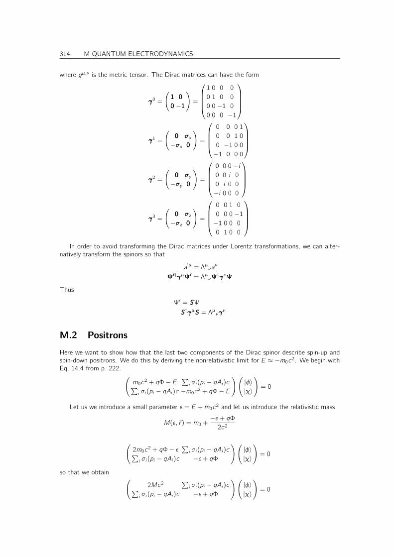
314 M QUANTUM ELECTRODYNAMICS
where gµ,ν is the metric tensor. The Dirac matrices can have the form
γ0 =
(111 000
000 −111
)=
1 0 0 0
0 1 0 0
0 0 −1 0
0 0 0 −1
γ1 =
(000 σx
−σx 000
)=
0 0 0 1
0 0 1 0
0 −1 0 0
−1 0 0 0
γ2 =
(000 σy
−σy 000
)=
0 0 0 −i0 0 i 0
0 i 0 0
−i 0 0 0
γ3 =
(000 σz
−σz 000
)=
0 0 1 0
0 0 0 −1
−1 0 0 0
0 1 0 0
In order to avoid transforming the Dirac matrices under Lorentz transformations, we can alter-
natively transform the spinors so that
a′µ = Λµνa
ν
ΨΨΨ′′′†γµΨΨΨ′′′ = ΛµνΨΨΨ†γνΨΨΨ
Thus
Ψ′ = SΨ
S†γµS = Λµνγν
M.2 Positrons
Here we want to show how that the last two components of the Dirac spinor describe spin-up andspin-down positrons. We do this by deriving the nonrelativistic limit for E ≈ −m0c
2. We begin withEq. 14.4 from p. 222. (
m0c2 + qΦ− E
∑i σi(pi − qAi)c∑
i σi(pi − qAi)c −m0c2 + qΦ− E
)(|φ〉|χ〉
)= 0
Let us we introduce a small parameter ε = E +m0c2 and let us introduce the relativistic mass
M(ε,~r) = m0 +−ε+ qΦ
2c2
(2m0c
2 + qΦ− ε∑
i σi(pi − qAi)c∑i σi(pi − qAi)c −ε+ qΦ
)(|φ〉|χ〉
)= 0
so that we obtain (2Mc2
∑i σi(pi − qAi)c∑
i σi(pi − qAi)c −ε+ qΦ
)(|φ〉|χ〉
)= 0

M QUANTUM ELECTRODYNAMICS 315
Now we use the first equation to express the electronic components by the positronic ones.
|φ〉 = −1
2Mc2
∑i
σi(pi − qAi)c |χ〉
and insert it into the second equation
0 =∑i
σi(pi − qAi)c |φ〉 − ε+ qΦ|χ〉
=
[−∑i
σi(pi − qAi)1
2M
∑i
σi(pi − qAi) + qΦ− ε
]|χ〉
= −
[∑i
σi(pi − qAi)1
2M
∑i
σi(pi − qAi)− qΦ + ε
]|χ〉
= −
[∑i
(pi − qAi)1
2M(pi − qAi) + i
∑i
σi
((~p − q ~A)×
1
2M(~p − q ~A)
)i
− qΦ + ε
]|χ〉
Now we are ready to form the non-relativistic limit. As c approaches infinity, the electroniccomponent |φ〉 goes to zero. The positronic components fulfil
0 =
[(~p − q ~A)2
2m0−q
m~B~S − qΦ + ε
]|χ〉
Let us compare this result with the Pauli equation for the electrons
0 =
[(~p − q ~A)2
2m0−q
m~B~S + qΦ− ε
]|φ〉
The equation for the positrons differs from that for the electrons by the sign reversal of the energyand the potential energy. In order to extract the implications for the dynamics, we use this equationto extract a classical Hamilton function. From that we can derive the classical equations of motionusing Hamilton’s equations.
One open problem is that we still have a two component spinor wave function. We want to avoidto deal with a classical spinor particle, even though such a generalization could be made. In orderto obtain two one-component wave functions, we restrict the equation to magnetic fields orientedalong the z-axis. In this case, the positronic Pauli equation separates exactly into one equation for

316 M QUANTUM ELECTRODYNAMICS
spin-up and one for spin-down positrons. nevertheless we keep the vector notation for ~S ~B.
Hp(~p,~r , t) = −
[(~p − q ~A)2
2m0−q
m~B~S − qΦ
].pi = −
∂H
∂ri=
[(~p − q ~A)
m0(−q∂i ~A)−
q
m(∂i ~B)~S − q∂iΦ
].r i =
∂H
∂pi= −
pi − qAim0
m0..r i = −.pi + q
.~r ~∇Ai + q∂tAi
= −
[(~p − q ~A)
m0(−q∂i ~A)−
q
m(∂i ~B)~S − q∂iΦ
]+ q
.~r ~∇Ai + q∂tAi
= −q.~r∂i ~A+
q
m(∂i ~B)~S + q∂iΦ + q
.~r ~∇Ai + q∂tAi
= −q [−∂iΦ− ∂tAi ]︸ ︷︷ ︸Ei
−q∑j
[.r j∂iAj −
.r j∂jAi
]︸ ︷︷ ︸
(~v×~B)i
−q
m(∂i ~B)~S
m0
..~r = −q
[~E + ~v × ~B
]−q
m(∂i ~B)~S
The first contribution is the Lorentz force acting on a particle with charge −q. The second part isthe force related to the energy of a particle with magnetic moment ~mp = q
m~S in a magnetic field ~B.
The energy of a magnetic moment ~m in a magnetic field ~B is E = −~m~B. The magnetic moment of aclassical charge distribution is ~m = g q
2m~L, where g is the g-factor, and ~L is the angular momentum.
Remember that the charge q of the electron is negative q = −e so that the charge of the positronis −q = +e, where e is the elementary charge.
Thus we can identify the Dirac spinor
|Ψ1〉 = |φ1〉 → e−↑
|Ψ2〉 = |φ2〉 → e−↓|Ψ3〉 = |χ1〉 → p↓
|Ψ4〉 = |χ2〉 → p↑
The positron pσ behaves exactly like an electron eσ with the opposite charge.

Mathematical appendices
317


Appendix N
Method of separation of variables
The method of separation of variables is a method to solve partial differential equations. While it isnot applicable only in a subset of systems, it leads to so dramatic simplification that it is usually thefirst method that is tried.
A simple example
Let us consider a simple example first, namely the one-dimensional wave equation
∂2xΦ(x, t) =
1
c2∂2t Φ(x, t)
We start with an product-Ansatz
Φ(x, t) = f (x)g(t)
During the calculation we have to verify if the Ansatz leads to a solution. If inconsistencies appear,we need to discard the Ansatz.
By dividing through the wave function we obtain
1
f (x)∂2x f (x) =
1
c2
1
g(t)∂2t g(t)
Since the right side does not depend on x , the left-hand side must be a constant. The analogousargument holds for the right-hand side. This allows us to break the problem up into two one-dimensional problems, namely
1
f (x)∂2x f (x) = C
1
c2
1
g(t)∂2t g(t) = C
which are two eigenvalue equations.
∂2x f (x) = Cf (x)
1
c2∂2t g(x) = Cg(x)
The breakup of the partial differential equation into several differential equations of lower dimension-ality is the essence of the method of separation of variables. The appearance of Eigenvalue equationsis also a fairly common feature of the method of separation of variables.
319

320 N METHOD OF SEPARATION OF VARIABLES
The method
The general idea of the method of separation of variables is to break up a partial differential equationinto problems of lower dimensionality. It starts with a ansatz of a product wave function.
While I am not sure if the following describes the complete class of problems to which the methodof separation of variables can be applied, it is by far the most common one.
The method of separation of variables works always, if the differential operator can be written asa sum of terms, where each only acts on a subset of the coordinates. In that case we can break thepartial differential equation into those subsets.
D(~∇x , ~∇y , ~x, ~y)Φ(~x, ~y) = 0
with
D(~∇x , ~∇y , ~x, ~y) = D1(~∇x , ~x) +D2(~∇y , ~y)
We choose the Ansatz
Φ(~x, ~y) = f (~x)g(~y)
and obtain [D1(~∇x , ~x) +D2(~∇y , ~y)
]f (~x)g(~y) = 0
1
f (~x)D1(~∇x , ~x)f (~x) +
1
g(~y)D2(~∇y , ~y)g(~y) = 0
The important step is that D1f g = gD1f and D2f g = f D2g, which is valid, because the differentialoperators do not act on the coordinates of the function, that is shifted in front of the expression.
This leads to
1
f (~x)D1(~∇x , ~x)f (~x) = C
1
g(~y)D2(~∇y , ~y)f (~y) = C
which is equivalent to two eigenvalue equations for the individual subsets
D1(~∇x , ~x)f ~x) = −Cf (~x)
D2(~∇y , ~y)g(~y) = Cg(~y)

Appendix O
Trigonometric functions
The zero’s of the cosine function lie at odd integer multiples of π2 and those of the sin function lie
at even multiples of π2 .
cos(x) = 0 ⇒ x =π
2(1 + 2k)
sin(x) = 0 ⇒ x =π
2(2k)
with integer k .The cosinus is an even function with respect to sign-change of the argument and the sinus is an
odd function
cos(x) = cos(−x)
sin(x) = − sin(x)
The formulas involving trigonometric functions appear quite complex and hard to memorize.However, they are extremely simple to derive, if one only considers them as real and imaginary partof the exponential function with imaginary argument.
One needs for this the identity
eix = cos(x) + i sin(x) (O.1)
the elementary rules for the exponential function
ex+y = exey
e0 = 1
∂xex = ex .
We start with the first formula that we will need frequently:
eixe−ix = ei0 = 1
1 =(
cos(x) + i sin(x))(
cos(x)− i sin(x))
= cos2(x) + sin2(x)
Thus we obtain
cos2(x) + sin2(x) = 1 (O.2)
The addition theorem is then obtained in the following way
ei(x+y) = eixeiy
cos(x + y) + i sin(x + y)Eq. O.1
=(
cos(x) + i sin(x))(
cos(y) + i sin(y))
= cos(x) cos(y)− sin(x) sin(y) + i(
cos(x) sin(y) + sin(x) cos(y))
321

322 O TRIGONOMETRIC FUNCTIONS
By comparing real and imaginary part individually we obtain
cos(x + y) = cos(x) cos(y)− sin(x) sin(y) (O.3)
sin(x + y) = cos(x) sin(y) + sin(x) cos(y) (O.4)
Similarly we obtain the square of sinus and cosinus as(eix)2
= e2ix(cos(x) + i sin(x)
)Eq. O.1
= cos(2x) + i sin(2x)
cos2(x)− sin2(x) + 2i sin(x) cos(x) = cos(2x) + i sin(2x) (O.5)
With the help of Eq. O.2 we can extract the square of cosinus and sinus functions from the realpart of the above identity.
cos2(x) =1
2
(cos2(x) + sin2(x)
)︸ ︷︷ ︸
=1
+1
2
(cos2(x)− sin2(x)
)︸ ︷︷ ︸
cos(2x)
=1
2
(1 + cos(2x)
)(O.6)
sin2(x) =1
2
(cos2(x) + sin2(x)
)︸ ︷︷ ︸
=1
−1
2
(cos2(x)− sin2(x)
)︸ ︷︷ ︸
cos(2x)
=1
2
(1− cos(2x)
)(O.7)
The derivatives are obtained as
deix
dx= ieix
d cos(x)
dx+ i
d sin(x)
dx= − sin(x) + i cos(x)
Thus we obtain
d cos(x)
dx= − sin(x)
d sin(x)
dx= + cos(x)

Appendix P
Gauss’ theorem
Gauss theorem says that the divergence of a vector field integrated over a volume is equal to thecomponent of the vector field normal to the surface integrated over the surface of the volume∫
Ω
dr∑i
∇i fi(r) =∑i
∫∂Ω
dAi fi(r) (P.1)
It is the multidimensional analogue of∫ b
a
dxdf
dx= f (b)− f (a)
A variant of Gauss’ theorem ∫Ω
dr∇ig(r) =
∫∂Ω
dAig(r) (P.2)
is obtained by using fi = eig(r), where ei = δi ,j is a unity vector pointing into the Cartesian directionj . ∫
Ω
dr∑i
∇i f (r) =
∫Ω
dr∑i
∇iδi ,jg(r) =
∫Ω
dr∇jg(r) =∑i
∫∂Ω
dAi fi(r)
=∑i
∫∂Ω
dAiδi ,jg(r) =
∫∂Ω
dAjg(r)
323

324 P GAUSS’ THEOREM

Appendix Q
Fourier transform
Q.1 General transformations
We would like to expand the function in a set of functions φi(x). This set of functions should becomplete so that any function f (x) is can be expressed as
f (x) =∑i
φi(x)Fi
We obtain the expansion coefficients fi in the following way. We pick one function out of the set,multiply the complex conjugate from the left and integrate∫
dx φ∗j (x)f (x) =∑i
[∫dx φ∗j (x)φi(x)
]Fi .
We construct an inverse U of the overlap matrix, so that∑k
Ui ,k
∫dx φ∗k(x)φj(x) = δi ,j .
Note that if functions in the set φi is overcomplete1, the matrix U is not uniquely defined andcannot be obtained using the conventional matrix inversion techniques. One way to obtain an inverseis singular value decomposition.
Then we multiply the matrix U from the left and obtain
Fi =∑j
Ui ,j
∫dx φ∗j (x)f (x)
Q.2 Fourier transform in an finite interval
Let us now consider a function f (x) that is defined on the interval [−L2 ,L2 ]. We choose a special set
of functions, namely φn(x) = CeiGnx , where GnL = 2πn and where C is an arbitrary constant.The overlap matrix is∫ L
2
− L2
dx φ∗n(x)φm(x) = C2
∫ L/2
−L/2
dx e−i(Gn−Gm)x = C2
∫ L/2
−L/2
dx ei2πL
(m−n)x = C2Lδn,m
1A set of functions is over complete, if one function out of the set can be represented as a linear superposition ofthe others.
325

326 Q FOURIER TRANSFORM
Being diagonal, the overlap matrix can be inverted easily so that
Fi =1
C2L
∫dx Ce−iGnx f (x) =
1
CL
∫dx e−iGnx f (x)
Forward an backward transform are therefore
f (x) = C∑n
eiGnxFn (Q.1)
Fn =1
CL
∫ L/2
−L/1
dx e−iGnx f (x) (Q.2)
with GnL = 2πn
The choice of the parameter C is arbitrary. The following choices are common.
• A good choice is C = 1, so that
f (x) =∑n
eiGnxFn
Fn =1
L
∫ L/2
−L/1
dx e−iGnx f (x)
• Often the symmetric form is preferred.
f (x) =
√1
L
∑n
eiGnxFn
Fn =
√1
L
∫ L/2
−L/1
dx e−iGnx f (x)
Q.3 Fourier transform on an infinite interval
Let us now consider the limit L → ∞. We introduce the spacing ∆ = 2πL between reciprocal lattice
points. Since this spacing vanishes in the limit of a large interval, we can convert the sum Eq. Q.1into an integral ∆
∑n →
∫dG of the continuous variable G.
f (x)Eq. Q.1
=C
∆
∫dG eiGxF (G) =
CL
2π
∫dG eiGxF (G)
F (G)Eq. Q.2
=1
CL
∫ L/2
−L/2
dx e−iGx f (x)
The limit can be performed if we keep β def= CL constant, while letting the interval L go to infinity.
f (x) = β
∫dG
2πeiGxF (G)
F (G) =1
β
∫dx e−iGx f (x)
Different conventions are in use:
• A symmetric form can be obtained by equating the pre factors for the forward and the backwardtransformation, that is β =
√2π.
f (x) =1√2π
∫dG eiGxF (G)
F (G) =1√2π
∫dx e−iGx f (x)

Q FOURIER TRANSFORM 327
• Personally, I prefer the non-symmetric version with β = 2π, which I am using in the presentlecture notes.
f (x) =
∫dG
2πeiGxF (G) (Q.3)
F (G) =
∫dx e−iGx f (x) (Q.4)
Q.4 Table of Fourier transforms
f (x) =∫dG2π eiGxF (G) F (G) =
∫dx e−iGx f (x)
δ(x) 1
eiG0x 2πδ(G − G0)
y(x − x0) y(G)e−iGx0∫dx ′g(x − x ′)y(x) g(G)y(G)
Q.5 Fourier transform of Dirac’s delta-function
Let us work out the Fourier transform of the delta function.The delta function is defined by the equation
f (x0) =
∫dx δ(x − x0)f (x) , (Q.5)
which must hold for all differentiable functions f (x).The Fourier transform of the δ-function is a a plane wave in reciprocal space, which is obtained
by using f (x) = e−iGx in Eq. Q.5. ∫dx δ(x − x0)e−iGx = e−iGx0 (Q.6)
If the delta function is located at the origin, i.e. x0 = 0, the Fourier transform is simply a constant.By comparing Eq. Q.6 with the equation for the Fourier transform Eq. Q.3 we identify F (G) =
e−iGx0 with the Fourier transform of the delta function. Inserting this into the backward transformEq. Q.3, we obtain the representation of the delta function as integral over reciprocal space
δ(x − x0) =
∫dG
2πeiG(x−x0)

328 Q FOURIER TRANSFORM

Appendix R
Pauli Matrices
All two-by-two matrices can be expressed as a superposition of the unity matrix and three Hermitiantwo-by-two matrices. These matrices are called Pauli matrices.
σx =
(0 1
1 0
); σy =
(0 −ii 0
); σz =
(1 0
0 −1
).
They play an important role for the description of the electron spin, for any two-state system andfor the quantum field theory of Fermions.
In order to become familiar with Pauli matrices, let us now investigate the commutator andanti-commutator relations. We use the multiplication table, which is obtained using the two-by-twomatrices
σjσj+1 = iσj+2
σjσj−1 = −iσj−2
σjσj = 111
where the j refers to the indices (x, y , z) with cyclic permutation. That is if j = y then j + 1 = zand j + 2 = x . etc.
The multiplication table has the form
σ1σ2 σx σy σz
σx 111 iσz -iσyσy -iσz 111 iσxσz iσy -iσx 111
where σ1 refers to the rows, and σ2 to the columns.The commutator table is obtained as the antisymmetric part of the multiplication table
[σ1σ2]− σx σy σz
σx 000 2iσz -2iσyσy -2iσz 000 2iσxσz 2iσy -2iσx 000
and the anti-commutator table is the symmetric part
[σ1σ2]+ σx σy σz
σx 222 000 000
σy 000 222 000
σz 000 000 222
.
329

330 R PAULI MATRICES
We can derive a very useful formula for Pauli matrices, namely
MAGIC FORMULA
(~A~σ)(~B~σ) = ~A~B + i~σ(~A× ~B (R.1)
which is proven in the following.Let us consider two superpositions of Pauli matrices
A =∑i
Aiσi = ~A~σ
B =∑i
Biσi = ~B~σ
The identity Eq. R.1 can be verified by using the multiplication table.
(~A~σ)(~B~σ) =∑j,k
AjBkσjσk
=∑j
AjBjσ2j +
∑j 6=k
AjBkσjσk
=∑j
AjBj +∑j 6=k
εj,k,lAjBk iσl
= ~A~B + i~σ(~A× ~B)
Hereby εi ,j,k is the completely antisymmetric tensor with εi ,j,k = 0 if any pair of the indices areequal. εi ,j,k = 1 if (i , j, k) is ascending, that is can be mapped onto the sequence (1, 2, 3, 1, 2), andεi ,j,k = −1 if (i , j, k) is descending, that is can be mapped onto the sequence (2, 1, 3, 2, 1). Thevector product can be written as (~A× ~B)i =
∑j,k εi ,j,kAjBk

Appendix S
Matrix identities
Editor: This whole chapter is in preparation
S.1 Notation
We introduce the complete orthonormal set of unit vectors
~ei
which have the components
(~e)i = ~ei~ej = δi ,j
S.2 Identities related to the trace
S.2.1 Definition
The trace of a matrix is defined as the sum of its diagonal elements.
Tr[A]def=∑i
Ai ,i =∑i ,j
δi ,jAi ,j (S.1)
A matrix can be written in the form
A = [~a1, ~a2, . . .]
where the vector components (~ai)j = Ai ,j or as
A = [∑i
~eiAi ,1,∑i
~eiAi ,2,∑i
~eiAi ,3, . . .] (S.2)
S.2.2 Invariance under commutation of a product
Tr[AB] = Tr[BA]
Proof:
Tr[AB] =∑i ,j
Ai ,jBj,i =∑i ,j
Bj,iAi ,jTr[BA]
331

332 S MATRIX IDENTITIES
S.2.3 Invariance under cyclic permutation
The trace is invariant under cyclic permutation
Tr[ABC] = Tr[CAB] (S.3)
The proof follows directly from the invariance of the trace under commutation of a product oftwo matrices: One simply considers the product AB as one matrix and C as the other.
S.2.4 Invariance under unitary transformation
The trace is invariant under transformation by a unitary matrix, i.e.
Tr[U†AU] = T r [A] (S.4)
Tr[U†AU] =∑i ,j,k
U†i ,jAj,kUk,i =∑i ,j,k
Uk,iU†i ,jAj,k = T r [UU†A]
UU†=111= T r [A]
S.3 Identities related to the determinant
S.3.1 Definition
The determinant is defined by the fully antisymmetric tensor ε as
det[A]def=∑i ,j,k,...
εi ,j,k,...Ai ,1Aj,2Ak,3 · · · (S.5)
The fully antisymmetric tensor has the following elements
•
ε1,2,3,... = 1
• The matrix element vanishes if two indices are equal.
• The matrix element changes its sign for every permutation of two indices
In the reverse the epsilon tensor can be expressed by the determinant by
det[~ei , ~ej , ~ek . . . , ]
]=
∑i ′,j ′,k ′,...
εi ′,j ′,k ′,...δi ′,iδj ′,jδk ′,k · · · = εi ,j,k,...
The determinant can also be written in the following form
det[A] =∑i ,j,k,...
εi ,j,k,...Ai ,1Aj,2Ak,3 · · · =∑i ,j,k,...
det[~ei , ~ej , ~ek , . . .]Ai ,1Aj,2Ak,3 · · ·
S.3.2 Product rule
det[AB] = det[A] det[B] (S.6)
S MATRIX IDENTITIES 333
Proof: The proof is taken from http://algebra.math.ust.hk/determinant/05_proof/lecture3.shtml#product. Fix the matrix A and consider
f (B)def= det[AB]
as a function of the matrix BLet us use the notation A = [~a1, ~a2, . . . , ~an] where a matrix is represented by its column vectors.A matrix product can then be written as
AB = [A~b1,A~b2 . . .]
Now we derive two properties of the function f , that we will need later:
1.
f ([. . . , ~u + ~v, . . .]) = det[A[. . . , ~u + ~v, . . .]) = det[[. . . ,A(~u + ~v), . . .]) = det[[. . . ,A~u + A~v, . . .])??= det[[. . . ,A~u, . . .]] + det[[. . . ,A~v, . . .]] = f ([. . . , ~u, . . .]) + f ([. . . , ~v , . . .])(S.7)
2.
f [(. . . , ~u, . . . , ~v , . . .]) = det[A · [. . . , ~u, . . . , ~v , . . .]] (S.8)
= det[[. . . ,A~u, . . . ,A~v, . . .]] (S.9)
= − det[[. . . ,A~v, . . . ,A~u, . . .]] (S.10)
= − det[A[. . . , ~v , . . . , ~u, . . .]] (S.11)
= −f [(. . . , ~v , . . . , ~u, . . .]) (S.12)
Thus we can write
f ([[[B])Eq. S.2
= f [∑i
~eiBi ,1,∑i
~eiBi ,2, . . .]
Eq. S.7=
∑i ,j,k,...
f [~ei , ~ej , . . .]Bi ,1Bj,2 · · · (S.13)
Now we interchange the unit vectors in f until they are in ascending order. According to Eq. S.12every interchange causes a sign change. The sign changes can be encoded by the fully antisymmetrictensor ε
f ([[[B])Eq. S.13
=∑i ,j,k,...
f [~ei , ~ej , . . .]Bi ,1Bj,2 · · ·
Eq. S.12=
∑i ,j,k,...
f [~e1, ~e2, . . .]εi ,j,k,...Bi ,1Bj,2 · · ·
= f [~e1, ~e2, . . .]︸ ︷︷ ︸det[A·111]
∑i ,j,k,...
εi ,j,k,...Bi ,1Bj,2 · · ·︸ ︷︷ ︸det[B]
= det[A] det[B]
Because f (B) = det[AB] this proves Eq. S.6.
S.3.3 Permutation of a product
Permutation of a product of two square matrices does not change the determinant
det[AB] = det[BA] (S.14)
The proof relies on the product rule Eq. S.6
det[AB]Eq. S.6
= det[A] det[B] = det[B] det[A]Eq. S.6
= det[BA]

334 S MATRIX IDENTITIES
S.3.4 1
det[ecA] = ecTr[A] (S.15)
Proof: Assuming that A can be diagonalized, let
A = U†aU (S.16)
where a is a diagonal matrix containing the eigenvalues of a, and U is a unitary matrix containingthe eigenvectors.
det[ecA] = det
[ ∞∑n=0
1
n!(cA)n
]Eq. S.16
= det
[ ∞∑n=0
1
n!
(U†caU
)n]U†U=111
= det
[U†
( ∞∑n=0
1
n!(ca)n
)U
]= det
[U†ecaU
]Eq. ??
= det[UU†eca
]U†U=111
= det [eca]
= eca11 · eca22 · · ·= eca11+ca22+···
= ecTr[a]
= ecTr[U†aU]
= ecTr[A]

Appendix T
Special Functions
Quantum mechanical problems often characterize special functions. A good source to find detailsabout them is Abramovitz Mathematical Tables and in a more accessible form the appendices ofMessiah Quantum Mechanics.
T.1 Bessel and Hankel functions
Bessel and Hankel functions play a role as radial part of the Schrödinger equation with a constantpotential.
T.2 Hermite Polynomials
Hermite polynomials are used to construct the solutions of the Schrödinger equation for the one-dimensional harmonic oscillator.
T.3 Legendre Polynomials
The Legendre polynomials appear in the θ dependence of spherical harmonics.
T.4 Laguerre Polynomials
(Source: Merzbacher)Laguerre Polynomials are are used for the solutions of the hydrogen atom.
[x∂2x + (1− x)∂x + n]Ln(x) = 0
Ln(0) = n!
The solutions are the Laguerre polynomials
Ln(x) = exdn
dxn
[xne−x
]= (−1 + ∂x)nxn
335

336 T SPECIAL FUNCTIONS
n Ln(x)
0 1
1 1− x2 x2 − 2x + 2
3 −x3 + 9x2 − 18x + 6
-4
-2
0
2
4
0 1 2 3 4 5 6 7 8
Fig. T.1: Laguerre polynomials rescaled so that the value at the origin is unity
Associated Laguerre Polynomials
[x∂2x + (m + 1− x)∂x + n −m]Lq(x) = 0
The associated Laguerre polynomials have the form
Lmn (x) = ∂mx Ln(x)
We start out with the radial Schrödinger equation for the Coulomb potential in Hartree atomicunits.
[−
1
2∂2r +
`(`+ 1)
2r2−Z
r− E
]r `+1e−λrF (r)
Now we use
∂r r`+1e−λr = r `+1e−λr
(`+ 1
r− λ+ ∂r
)∂2r r`+1e−λr = r `+1e−λr
(`+ 1
r− λ+ ∂r
)2
(`+ 1
r− λ+ ∂r
)2
= ∂2r −
`+ 1
r2+ 2(`+ 1
r− λ
)∂r +
(`+ 1
r− λ
)2
= ∂2r + 2
(`+ 1
r− λ
)∂r −
`+ 1
r2+
(`+ 1)2
r2− 2λ
`+ 1
r+ λ2
= ∂2r + 2
(`+ 1
r− λ
)∂r +
`(`+ 1)
r2− 2λ
`+ 1
r+ λ2

T SPECIAL FUNCTIONS 337
Now we insert this to obtain an equation for F (r)[(∂2r + 2
(`+ 1
r− λ
)∂r +
`(`+ 1)
r2− 2λ
`+ 1
r+ λ2
)−`(`+ 1)
r2+
2Z
r+ 2E
]F (r) = 0[
r∂2r +
(2(`+ 1)− 2λr
)∂r +
(2Z − 2λ(`+ 1)
)+ r(
2E + λ2)]F (r) = 0[
x∂2x +
(2(`+ 1)− x
)∂x +
(Zλ− (`+ 1)
)+
r
2λ
(2E + λ2
)]F (x/(2λ) = 0
Now we select λ =√−2E and obtain
[x∂2
x +(
2(`+ 1)− x)∂x +
(Zλ− (`+ 1)
)]F (x/(2λ) = 0
Now we set p + 1 = 2(` + 1) and q − p =√Z2−2E − ` − 1 and obtain ... with p = 2` + 1 and
q =√Z2−2E + `. In order to obtain an integer solution for q we need
E = −Z2
2n2
with n = q − ` or q = n + `.Thus the solution is
R(r) = L2`+1n+` (2λr)r `e−λr
λ =√−2En =
Z
n
For n =√
Z2
−2E the solutions are the associated Laguerre polynomials F (x/√−2E) = L`n(x)

338 T SPECIAL FUNCTIONS

Appendix U
Principle of least action for fields
Now let us generalize the Formalism of least action to fields: in general we have now a Lagrangiandensity that depends on the field amplitudes φ(x, t), their time and spatial derivatives1 ∂tφ and ∂xφrespectively and of course on time and spatial coordinates.
L(φ, ∂tφ, ∂xφ, x, t)
The action is a functional of the field
S([φ(x, t], x, t) =
∫dt
∫dxL(φ, ∂tφ, ∂xφ, x, t)
The Euler-Lagrange equations are obtained from the variation of φ(x, t) by δφ(x, t), which yields
δS([φ(x, t], x, t) =
∫dt
∫dx[ dLdφ(x, t)
δφ(x, t) +dL
d∂tφ(x, t)δ∂tφ(x, t)
+dL
d∂xφ(x, t)δ∂xφ(x, t)
]=
∫dt
∫dxδφ(x, t)
[ dLdφ(x, t)
− ∂tdL
d∂tφ(x, t)− ∂x
dLd∂xφ(x, t)
]We have used Gauss theorem, and the requirement that the variation of the field vanishes at theintegration boundary, that is at ti and tf and at x = ±∞.
The resulting Euler-Lagrange equations are
∂tdL
d∂tφ(x, t)=
dLdφ(x, t)
− ∂xdL
d∂xφ(x, t)
We can also derive the Hamilton equations by a Legendre transform of the Lagrangian. We firstintroduce a field momentum density
Π(x, t) =δLδ∂tφ
The field momentum has a different physical meaning than the momentum of mass particles, eventhough formally they are equivalent.
Next define a Hamilton function
H([Π(x, t)], [φ(x, t)], x, t) =
∫dx[
Π(x, t)∂tφ(x, t)− L]
1There may be more than one spatial derivatives but we remain here consistent with the one-dimensional description.The generalization is obtained by indexing the spatial coordinates and introducing more of them.
339

340 U PRINCIPLE OF LEAST ACTION FOR FIELDS
We consider the derivatives of the field amplitudes as independent variables.The derivative of theright hand side with respect to ∂tφ, vanishes if the Momenta are defined as above.
Let us now consider the derivatives with respect to field amplitudes and momenta.
δHδΠ(x, t)
= ∂tφ(x, t)
δHδφ(x, t)
= −∂L∂φ

Appendix V
`-degeneracy of the hydrogen atom
For the hydrogen atom, the eigenvalues depend only on the main quantum number, but the eigen-values with the same main angular momenta are degenerate. This degeneracy is not a consequenceof rotational symmetry. Rotational symmetry only leads to degenerate eigenvalues with differentmagnetic quantum numbers m. The `-degeneracy is peculiar1 for the non-relativistic Schrödingerequation with a Coulomb potential. It is not caused by a geometric symmetry but a so-called dy-namical symmetry. A symmetry is called dynamical if it originates from the equations of motionand not directly from a space-time symmetry.
I am following a description[51] by M. Jacobi and H. Spahr taken from http://www.desy.de/~jlouis/Vorlesungen/QMII06/vortrag_09.pdf.
V.1 Laplace-Runge-Lenz Vector
The non-relativistic electron in a hydrogen atom experiences a potential that is analogous to theKepler problem. The Hamilton operator has the form
H =~p2
2m−κ
|~r |(V.1)
where κ = Ze2
4πε0for the hydrogen atom.
The classical Kepler problem has a conserved quantity, called the Laplace-Runge-Lenz vector
~Mdef=
1
2m
(~p × ~L− ~L× ~p
)−κ
|~r |~r (V.2)
This is already the hermitian translation of the classical Runge-Lenz vector.The classical Laplace-Runge-Lenz vector lies in the plane of the trajectory and points along the
principal axis of the ellipse. Conservation of the Runge-Lenz vector implies that the trajectory isa ellipse that is stationary in space. For general spherical potentials there will be a precession ofapsides2 of any orbit. The observation of the precession of the apsides of Mercury has been onesupporting experimental evidence for the general theory of relativity, as it was a prove for a deviationof the gravitational force from the pure 1/r form.
The Runge-Lenz vector is a constant of motion:
[ ~M, H]Eq. V.45
= 0 (V.3)1Also the spherical harmonic oscillator in three dimensions exhibits `-degeneracy.2The apsides are the point of smallest and farthest distance from the system’s center of gravity. Singular: apsis,
plural apsides. The point of closest approach is called periapsis or pericenter. The point of farthest distance is calledapoapsis or apocenter. The perihelion is the periapsis of an orbit about the sun.
341

342 V `-DEGENERACY OF THE HYDROGEN ATOM
V.1.1 Commutator relations of Runge-Lenz vector and angular momentum
[Li , Lj ] = i~∑k
εi ,j,k Lk (V.4)
[Mi , Lj ]Eq. V.53
= i~∑k
εi ,j,kMk (V.5)
[Mi , Mj ]Eq. V.54
= i~−2H
m
∑k
εi ,j,k Lk (V.6)
V.1.2 Rescale to obtain a closed algebra
The operators ~M and ~L would form a closed algebra, if the Hamilton operator would not appear inthe last expression Eq. V.6. Because the Hamiltonian commutates with the Runge-Lenz vector, wecan define a new operator
~M ′def= i
√m
2H−
12 ~M (V.7)
This expression is defined because Hamilton operator and Runge-Lenz vector commutate. Thus, foreach cartesian direction, I can determine a common system of eigenstates |n〉 with
H|n〉 = |n〉εnMi |n〉 = |n〉an
Then I can write the operator
M ′i =
√m
2
∑n
|n〉an√−εn〈n|
Note, that the eigensystem n is different for the three components of ~M ′, because the differentcomponents of ~M do not commutate. The new operator is not hermitian, because it has imaginaryeigenvalues for states with positive energy.
Because the Hamiltonian commutates with the Runge-Lenz vector and with the angular momen-tum, we can easily adapt the commutator relations to the ones for the scaled vector ~M ′.
[Li , Lj ] = i~∑k
εi ,j,k Lk
[M ′i , Lj ]Eq. V.5
= i~∑k
εi ,j,kM ′k (V.8)
[M ′i , M ′j ]Eq. V.6
= i~∑k
εi ,j,k Lk (V.9)
V.2 SO(4) symmetry
One introduces the generalized angular momenta
~J(1) def=
1
2
(~L+ ~M ′
)(V.10)
~J(2) def=
1
2
(~L− ~M ′
)(V.11)

V `-DEGENERACY OF THE HYDROGEN ATOM 343
These operators obey the following commutator relations that have been derived in Eq. V.56
[J(1)i , J
(1)j ] = i~
3∑k=1
εi ,j,k J(1)k (V.12)
[J(2)i , J
(2)j ] = i~
3∑k=1
εi ,j,k J(2)k (V.13)
[J(1)i , J
(2)j ] = 0 (V.14)
This algebra is can be characterized[51] as SO(3)×SO(3), as SU(2)×SU(2), or as SO(4).SO(d) stands for special orthogonal group in d dimensions. It is the group of real d × d matrices
with determinant +1. These matrices are the rotation matrices in d dimensions. In d dimensionsthere are 1 + 2 + . . .+ (d − 1) = d(d−1)
2 independent rotation axes corresponding to the independentmatrix elements in an antisymmetric matrix in d dimensions. The antisymmetric matrices are thegenerators of this group.
SU(d) stands for special unitary group. It is the group of complex d×d matrices with determinant+1.
The SO(4) symmetry corresponds to rotations in a four-dimensional cartesian space. In fourdimensions, there are six rotation angles. These rotations do not operate in some physical space.
V.3 `-Degeneracy of the hydrogen atom
In order to make the link to the `-degeneracy, we show that the Hamiltonian of the hydrogen atomcan be expressed entirely by the generalized angular momenta ~J(1) and ~J(2).
~M2 Eq. V.39=
2
mH(~L2 + ~2
)+ κ2
⇒ −m
2H−1 ~M2 + ~L2 + ~2 = −
m
2κ2H−1
Eq. V.7⇒ ~M′2 + ~L2 + ~2 = −
m
2κ2H−1
Eqs. V.10,V.11⇒ 2
[(~J(1))2
+(~J(2))2]
+ ~2 = −m
2κ2H−1
Thus we can express the Hamiltonian by the squares of the generalized angular momenta ~J(1) and~J(2).
⇒ H = −mκ2
2
[2(~J(1))2
+ 2(~J(2))2
+ ~2
]−1
(V.15)
Each of the operators ~J(1) and ~J(2) obeys an algebra that is identical to the angular momentumalgebra, which has been obtained for the normal angular momentum ~L. Therefore, we obtain thesame eigenvalue spectrum, namely(
~J(1))2
|j1, j2〉 = |j1, j2〉~2j1(j1 + 1) (V.16)(~J(2))2
|j1, j2〉 = |j1, j2〉~2j2(j2 + 1) (V.17)
where j1 and j2 may be non-negative, half-integer numbers

344 V `-DEGENERACY OF THE HYDROGEN ATOM
With Eq. V.55 we can show that the j1 = j2def= j .
0Eq. V.55
= ~M ′~L|j1, j2〉Eq. V.11
=(~J(1) − ~J(2)
)(~J(1) + ~J(2)
)|j1, j2〉
Eq. V.17=
(~J(1) − ~J(2)
)|j1, j2〉~2 [j1(j1 + 1) + j2(j2 + 1)]
Eq. V.17= |j1, j2〉~2 [j1(j1 + 1)− j2(j2 + 1)] ~2 [j1(j1 + 1) + j2(j2 + 1)]
⇒ j1 = j2 ∧ j1 = −(j2 + 1)
Since j1 and j2 are non-negative, we can conclude that the two parameters are identical.Now return to Eq. V.15 and determine the eigenvalues
H|j〉 Eq. V.15= −
mκ2
2
[2(~J(1))2
+ 2(~J(2))2
+ ~2
]−1
|j〉
= |j〉[−mκ2
2
[4~2j(j + 1) + ~2
]−1]
= |j〉[−mκ2
2~2[2j + 1]−2
]Thus we obtain the eigenvalues
Enndef=2j+1
= −mκ2
2~2
1
n2
This is the eigenvalue spectrum of the hydrogen atom. We can form a basisset(~J(1))2
|j, m1, m2〉 = |j, m1, m2〉~2j(j + 1)
~J(1)z |j, m1, m2〉 = |j, m1, m2〉~m1
~J(2)z |j, m1, m2〉 = |j, m1, m2〉~m2
because(~J(1))2
, ~J(1)z and ~J(1)
z form with the Hamiltonian a set of mutually commutating operators.
Because the energy depends only on j , there are (2j + 1)2 pairs of quantum numbers (m1, m2).Hence each eigenvalue has a degeneracy n2, which is exactly the degeneracy predicted for the hydro-gen atom including `-degeneracy.
V.4 Derivation of commutator relations used in this chapter
Here I shall in future include the derivation of the expressions used above: These calculations are notfinished. The derivations are from http://www.theochem.ru.nl/~pwormer/rungelenz.pdf[52].
This derivation is not completed!!!!
[pi , Lj ] =∑m,n
εj,m,n[pi , xmpn] =∑m,n
εj,m,n (pi xmpn − xmpnpi)
=∑m,n
εj,m,n
~iδi ,mpn + xmpi pn − xmpnpi︸ ︷︷ ︸
=0
=~i
∑n
εj,i ,npn
= i~∑k
εi ,j,k pk (V.18)

V `-DEGENERACY OF THE HYDROGEN ATOM 345
[xi , Lj ] =∑m,n
εj,m,n[xi , xmpn] =∑m,n
εj,m,n (xi xmpn − xmpnxi)
=∑m,n
εj,m,n
(xi xmpn − xm
~iδn,i − xmxi pn
)= i~
∑k
εi ,j,k xk (V.19)
~L~p =∑i ,j,k
εi ,j,k︸︷︷︸=−εk,j,i
xj pkpi︸︷︷︸pipk
= 0 (V.20)
~L(~L× ~p) =∑i ,j,k
εi ,j,k︸︷︷︸=−εj,i ,k
LiLj︸︷︷︸=LjLi
pk = 0 (V.21)
~L(~p × ~L) =∑i ,j,k
εi ,j,kLipjLk
Eq. V.18=
∑i ,j,k
εi ,j,kLi
(i~∑m
εj,k,mpm
)+∑i ,j,k
εi ,j,kLiLkpj︸ ︷︷ ︸=0
= i~∑i ,m
∑j,k
εi ,j,kεm,j,k
︸ ︷︷ ︸
2δi ,m
Lipm = i~~L~p Eq. V.20= 0 (V.22)
~L~r
|~r | =∑i ,j,k
εi ,j,kxjpkxi1
|~r | =∑i ,j,k
εi ,j,kxj~iδi ,k
1
|~r | +∑i ,j,k
εi ,j,kxjxipk1
|~r |
=~i
∑j,j
εi ,j,i︸︷︷︸=0
xj1
|~r | +∑i ,j,k
εi ,j,k=−εj,i ,k xjxi︸︷︷︸=xixj
pk1
|~r | = 0 (V.23)
~L ~MEq. V.2
= ~L
[1
2m
(~p × ~L− ~L× ~p
)−κ
|~r |~r
]
=1
2m
~L(~p × ~L)︸ ︷︷ ︸=0
− ~L(~L× ~p)︸ ︷︷ ︸=0
− κ ~L ~r|~r |︸︷︷︸
=0
Eqs. V.21,V.22,V.23= 0 (V.24)

346 V `-DEGENERACY OF THE HYDROGEN ATOM
(~L× ~p
)i
=∑j,k
εi ,j,k Lj pk
=∑j,k
εi ,j,k pk Lj −∑j,k
εi ,j,k [pk , Lj ]
Eq. V.18= −
∑j,k
εi ,j,k pj Lk − i~∑j,k
εi ,j,k∑m
εk,j,mpm
= −∑j,k
εi ,j,k pj Lk − i~∑m
−∑j,k
εi ,j,kεm,j,k
︸ ︷︷ ︸
2δi ,m
pm
= −(~p × ~L
)i
+ 2i~pi (V.25)
~p(~p × ~L) =∑i ,j,k
εi ,j,k︸︷︷︸=−εj,i ,k
pipj︸︷︷︸=pjpi
Lk = 0 (V.26)
~p(~L× ~p)Eq. V.25
= ~p[−(~p × ~L) + 2i~~p
]Eq. V.26
= 2i~~p2 (V.27)
(~p × ~L)~p =∑i ,j,k
εi ,j,kpjLkpi =∑i ,j,k
εj,k,ipjLkpi = ~p(~L× ~p)
Eq. V.27= 2i~~p2 (V.28)
V.4.1 Calculation of ~M2
Products of ~p × ~L and ~L× ~p
(~p × ~L)2 =∑
i ,j,k,m,n
εi ,j,kεi ,m,npjLkpmLn =∑j,k,m,n
(∑i
εi ,j,kεi ,m,n
)︸ ︷︷ ︸δj,mδk,n−δj,nδk,m
pjLkpmLn
=∑j,k
(pjLkpjLk − pjLkpkLj)
=∑j,k
(pj [Lk , pj ]Lk + pjpjLkLk − pjLkpkLj)
Eq. V.18= i~
∑i ,j,k
εk,j,i︸︷︷︸=−εk,i ,j
pjpi︸︷︷︸=pipj
Lk + ~p2~L2 −∑j
pj (~L~p)︸︷︷︸=0
Lj
Eq. V.20= ~p2~L2 (V.29)
This is the result of Eq. 15 of Wormer[52].

V `-DEGENERACY OF THE HYDROGEN ATOM 347
(~p × ~L)(~L× ~p)Eq. V.25
= (~p × ~L)[−~p × ~L+ 2i~~p
]Eq. V.29
= −~p2~L2 + 2i~(~p × ~L)~p
= −~p2~L2 + 2i~∑i ,j,k
εi ,j,kpjLkpi
= −~p2~L2 + 2i~∑i ,j,k
εj,k,ipjLkpi = −~p2~L2 + 2i~ ~p(~L× ~p)︸ ︷︷ ︸2i~~p2
(V.30)
Eq. V.27= −~p2~L2 − 4~2~p2 (V.31)
This is the result of Eq. 18 of Wormer[52].
(~L× ~p)(~p × ~L)Eq. V.25
=[−~p × ~L+ 2i~~p
](~p × ~L)
Eq. V.29= −~p2~L2 + 2i~ ~p(~p × ~L)︸ ︷︷ ︸
=0
Eq. V.26= −~p2~L2 (V.32)
This is the result of Eq. 16 of Wormer[52].
(~L× ~p)(~L× ~p)Eq. V.25
=[−~p × ~L+ 2i~~p
] [−~p × ~L+ 2i~~p
]Eq. V.29
= ~p2~L2 − 2i~
(~p × ~L)~p︸ ︷︷ ︸2i~~p2
+ ~p(~p × ~L)︸ ︷︷ ︸=0
− 4~2 ~p2
Eq. V.28,V.26= ~p2~L2 (V.33)
This is the result of Eq. 17 of Wormer[52].We can combine these four results to(
~p × ~L− ~L× ~p)2
= ~p2~L2 − (−~p2~L2 − 4~2~p2)− (−~p2~L2) + ~p2~L2
= 4~p2(~L2 + ~2
)(V.34)
(~L× ~p)~r
|~r | =∑i ,j,k
εi ,j,kLjpkxi1
|~r |
=∑i ,j,k
εi ,j,kLj~iδk,i
1
|~r | +∑i ,j,k
εi ,j,kLjxipk1
|~r |
=∑i ,j,k
εi ,j,i︸︷︷︸=0
Lj~i
1
|~r | +∑j
Lj∑i ,k
εj,k,ixipk︸ ︷︷ ︸=−Lj
1
|~r |
= −~L2
|~r | (V.35)
This is the result of Eq. 19 of Wormer[52]. Note that ~L2 commutates with any spherical function of~r .

348 V `-DEGENERACY OF THE HYDROGEN ATOM
(~p × ~L)~r
|~r |Eq. V.25
= −(~L× ~p)~r
|~r | + 2i~~p~r
|~r |Eq. V.35
=~L2
|~r | + 2i~~p~r
|~r | (V.36)
This is the result of Eq. 20 of Wormer[52].
~r
|~r |(~p ×~L) =
1
|~r |∑i ,j,k
εi ,j,kxipjLk =1
|~r |~L2 (V.37)
This is the result of Eq. 21 of Wormer[52].
~r
|~r |(~L× ~p)
Eq. V.25=
~r
|~r |
(−~p × ~L+ 2i~~p
)= −
~r
|~r |
(~p × ~L
)+ 2i~
~r
|~r |~p
Eq. V.37= −
~L2
|~r |+ 2i~
1
|~r |~r ~p (V.38)
This is the result of Eq. 22 of Wormer[52].
~M2 Eq. V.2=
[1
2m
(~p × ~L− ~L× ~p
)−κ
|~r |~r
]2
=1
4m2
(~p × ~L− ~L× ~p
)2
︸ ︷︷ ︸Eq. V.34
−κ
2m
(~p × ~L− ~L× ~p
)( ~r
|~r |
)︸ ︷︷ ︸
Eq. V.36 and Eq. V.35
−κ
2m
(~r
|~r |
)(~p × ~L− ~L× ~p
)︸ ︷︷ ︸
Eq. V.37 and Eq. V.38
+κ2
(~r
|~r |
)2
=1
4m2
(4~p2
[~L2 + ~2
])−
κ
2m
(2~L2
|~r | + 2i~~p~r
|~r |
)−
κ
2m
(2~L2
|~r | − 2i~~r
|~r |~p
)+ κ2
=1
4m2
(4~p2
[~L2 + ~2
])−
κ
2m4~L2
|~r | −κ
2m2i~[~p,
~r
|~r | ] + κ2
=1
4m2
(4~p2
[~L2 + ~2
])−
κ
2m4~L2
|~r | −κ
2m2~2
(3
|~r | −1
|~r |3~r2
)+ κ2
=2
m
(~p2
2m
[~L2 + ~2
])−
κ
2m4~L2
|~r | −2~2
m
κ
|~r | + κ2
=2
m
~p2
2m
[~L2 + ~2
]−
2
m
κ
|~r |~L2 −
2
m
κ
|~r |~2 + κ2
=2
m
(~p2
2m−κ
|~r |
)[~L2 + ~2
]+ κ2
Eq. V.1=
2
mH[~L2 + ~2
]+ κ2 (V.39)
This is the third statement or Theorem 2 of Wormer[52].

V `-DEGENERACY OF THE HYDROGEN ATOM 349
V.4.2 Commutator of ~M and ~H
([~p × ~L, ~p2]
)i
=∑i ,j,k
εi ,j,k(pjLkp
2m − p2
mpjLk)
=∑i ,j,k
εi ,j,k (pj(Lkpm)pm − pjpm(pmLk))
=∑i ,j,k
εi ,j,k (pj [Lk , pm]pm + pjpmLkpm − pjpm[pm, Lk ]− pjpmLkpm)
=∑i ,j,k
εi ,j,k (−pj [pm, Lk ]pm − pjpm[pm, Lk ])
Eq. V.18= −
∑i ,j,k
εi ,j,kpjpm
(i~∑n
εm,k,npn
)
= −i~∑i ,j,n
(∑k
εk,i ,jεk,n,m
)︸ ︷︷ ︸
δi ,nδj,m−δi ,mδj,n
pjpmpn
= −i~
∑j
pjpjpi −∑j
δj,npjpipj
= 0 (V.40)
(~r × ~L
)i
=∑j,k
εi ,j,kxjLk =∑j,k
εi ,j,kxj∑m,n
εk,m,nxmpn =∑j,n,m
(∑k
εk,i ,jεk,m,n
)︸ ︷︷ ︸
δi ,mδj,n−δi ,nδj,m
xjxmpn
=∑j,n,m
δi ,mδj,nxjxmpn −∑j,n,m
δi ,nδj,mxjxmpn =∑j
(xjxipj − xjxjpi)
=(~r(~r ~p)− ~r2~p
)i
(V.41)
This is the result of Eq. 23 of Wormer[52].
(~L× ~r
)i
=∑j,k
εi ,j,kLjxk =∑j,k
εi ,j,k∑m,n
εj,m,nxmpnxk =∑k,n,m
∑j
εj,k,iεj,m,n
︸ ︷︷ ︸
δk,mδi ,n−δk,nδi ,m
xmpnxn
=∑k,n,m
δk,mδi ,nxmpnxk −∑k,n,m
δk,nδi ,mxmpnxk =∑k
(xkpixk − xipkxk)
=∑k
(−~iδk,ixk + pixkxk +
~iδi ,kxk − pkxkxi) =
∑k
(pixkxk − pkxkxi)
=(~p~r2 − (~p~r)~r
)i
(V.42)
This is the result of Eq. 24 of Wormer[52].

350 V `-DEGENERACY OF THE HYDROGEN ATOM
[pi ,xj|~r | ] =
~i
(δi ,j|~r | −
xixj|~r |3
)
→ [p2,xj|~r | ] =
∑i
pipi xj|~r −pi xj|~r pi + pixj|~r pi︸ ︷︷ ︸
=0
−xj|~r pipi
=
∑i
(pi [pi ,
xj|~r ] + [pi ,
xj|~r ]pi
)=
~i
∑i
(pi
(δi ,j|~r | −
xixj|~r |3
)+
(δi ,j|~r | −
xixj|~r |3
)pi
)=
~i
(pj~r
2 1
|~r |3 − (~p~x)xj|~r |3 +
1
|~r |3~r2pj −
xj|~r |3 (~x~p)
)
=~i
(pj~r2 − (~p~x)xj)︸ ︷︷ ︸
=(~L×~r)j
1
|~r |3 +1
|~r |3(~r2pj − xj(~x~p)
)︸ ︷︷ ︸−(~r×~L)j
Eqs. V.42,V.41
=~i
[(~L× ~r)j
1
|~r |3 −1
|~r |3 (~r × ~L)j
][~r ,|~r |−3]=0;[~L,|~r |−3]=0
=i~|~r |3
(~r × ~L− ~L× ~r
)j
(V.43)
([1
r, ~L× ~p − ~p × ~L]
)i
=∑j,k
εi ,j,k
(1
|~r |(Ljpk − pjLk)− (Ljpk − pjLk)1
|~r |
)[~L,|~r |−1]=0
=∑j,k
εi ,j,k
(Lj
1
|~r |pk −1
|~r |pjLk − Ljpk1
|~r | + pj1
|~r |Lk)
=∑j,k
εi ,j,k
(−Lj [pk ,
1
|~r | ] + [pj ,1
|~r | ]Lk)
=~i
∑j,k
εi ,j,k
(+Lj
xk|~r |3 −
xk|~r |3 pj
)
=~i
(+~L×
~r
|~r |3 −~r
|~r |3 ×~L
)j
[~L,|~r |−3]=0=
~i
1
|~r |3(~L× ~r − ~r × ~L
)j
(V.44)
This is the result of Lemma 10 of Wormer[52].

V `-DEGENERACY OF THE HYDROGEN ATOM 351
[ ~M, H]Eq. V.1,V.2
=
[1
2m
(~p × ~L− ~L× ~p
)−κ
|~r |~r,~p2
2m−κ
|~r |
]−
=1
4m2
[(~p × ~L− ~L× ~p
), ~p2]−︸ ︷︷ ︸
=0 (Eq. V.40,Eq. V.25)
−κ
2m
[(~p × ~L− ~L× ~p
),
1
|~r |
]−︸ ︷︷ ︸
Eq. V.44
−κ
2m
[~r
|~r |, ~p2
]−︸ ︷︷ ︸
Eq. V.43
+κ2
[~r
|~r |,
1
|~r |
]−︸ ︷︷ ︸
=0
= −κ
2m
~i
1
|~r |3(~L× ~r − ~r × ~L
)−
κ
2m
−i~|~r |3
(~r × ~L− ~L× ~r
)= 0 (V.45)
V.4.3 Commutators of ~M and ~L
[(~L× ~p)i , (~L× ~p)j ] =∑k,l
∑m,n
εi ,k,lεj,m,n (LkplLmpn − LmpnLkpl) (V.46)
=∑k,l
∑m,n
εi ,k,lεj,m,n (Lk [pl , Lm]pn − Lm[pn, Lk ]pl) (V.47)
=∑k,l
∑m,n
εi ,k,lεj,m,n
(Lk
(i~∑o
εl ,m,opo
)pn − Lm
(i~∑o
εn,k,opo
)pl
)= i~
∑k,l,m,n,o
(εi ,k,lεj,m,nεl ,m,oLkpopn − εi ,k,lεj,m,nεn,k,oLmpopl) (V.48)
= i~∑k,l,o
(∑n
εi ,k,l
(∑m
εm,n,jεm,o,l
)Lkpopn −
∑m
εi ,k,l
(∑n
εj,m,nεn,k,o
)Lmpopl
)
= i~∑k,l,o
(∑n
εi ,k,l (δn,oδj,l − δn,lδj,o)Lkpopn −∑m
εi ,k,l (δj,kδm,o − δj,oδm,k)Lmpopl
)= i~
∑k,l,o
(∑n
εi ,k,lδn,oδj,lLkpopn −∑n
εi ,k,lδn,lδj,oLkpopn
−∑m
εi ,k,lδj,kδm,oLmpopl +∑m
εi ,k,lδj,oδm,kLmpopl
)
= i~
∑k,n
εi ,k,jLkpnpn −∑k,n
εi ,k,nLkpjpn︸ ︷︷ ︸(A)
−∑l ,m
εi ,j,lLmpmpl +∑l ,m
εi ,m,lLmpjpl︸ ︷︷ ︸(A)
= −i~
(∑k
εi ,j,kLk~p2 − (~L~p)
∑k
εi ,j,kpk
)= −i~
∑k
εi ,j,k
(Lk~p
2 − (~L~p)pk
)(V.49)
This differs from the corresponding result of Lemma 12 of Wormer[52].

352 V `-DEGENERACY OF THE HYDROGEN ATOM
[(~p × ~L)i , (~p × ~L)j ] =∑k,l,m,n
εi ,k,lεj,m,n(pkLlpmLn − pmLnpkLl)
=∑k,l,m,n
εi ,k,lεj,m,n(pk [Ll , pm]Ln + pkpmLlLn − pm[Ln, pk ]Ll − pmpkLnLl)
Eq. V.18=
∑k,l,m,n
εi ,k,lεj,m,n
(pk
(−i~
∑o
εm,l,o po
)Ln − pm
(−i~
∑p
εk,n,ppp
)Ll
)
= −i~∑k,l,m,n
εi ,k,lεj,m,n
(∑o
εm,l,opk poLn −∑p
εk,n,ppmppLl
)
= −i~
(∑k,n,o
(∑l
εi ,k,l∑m
εm,n,jεm,l,o
)pk poLn −
∑l ,m,o
(∑k
εi ,k,l∑n
εn,j,mεn,o,k
)pmpoLl
)
= −i~(∑k,n,o
(∑l
εi ,k,l (δn,lδj,o − δn,oδj,l)
)pk poLn
−∑l ,m,o
(∑k
εi ,k,l (δj,oδm,k − δj,kδm,o)
)pmpoLl
)= −i~
(∑k,n
εi ,k,npk pjLn −∑k,n
εi ,k,jpk pnLn −∑l ,m
εi ,m,lpmpjLl +∑l ,m
εi ,j,lpmpmLl
)
= −i~
∑k,n
εi ,k,npk pjLn︸ ︷︷ ︸(A)
−∑k,n
εi ,k,jpk pnLn −∑k,n
εi ,k,npk pjLn︸ ︷︷ ︸(A)
+∑k,n
εi ,j,npk pkLn
= −i~
(+∑k,n
εi ,j,kpk(~p~L) + ~p2∑n
εi ,j,nLn
)(V.50)
[(~p × ~L)i , pj ] =∑m,n
εi ,m,n(pmLnpj − pjpmLn) =∑m,n
εi ,m,n(pm[Ln, pj ] + pmpjLn − pjpmLn︸ ︷︷ ︸=0
)
Eq. V.18=
∑m,n
εi ,m,npm
(−i~
∑k
εj,n,k pk
)
= −i~∑k,m
(∑n
εn,i ,mεn,k,j
)pmpk
= −i~∑k,m
(δi ,kδm,j − δi ,jδm,k) pmpk
= −i~(pi pj − δi ,j~p2
)(V.51)
[(~p × ~L)i , (~L× ~p)j ]Eq. V.25
= −[(~p × ~L)i , (~L× ~p)j ] + 2i~[(~p × ~L)i , pj ]
Eqs. V.50,V.51= i~
(+∑k,n
εi ,j,kpk(~p~L) + ~p2∑n
εi ,j,nLn
)+ 2i~
(−i~
(pi pj − δi ,j~p2
))= i~
∑k,n
εi ,j,kpk(~p~L) + i~~p2∑n
εi ,j,nLn + 2~2(pi pj − δi ,j~p2
)(V.52)

V `-DEGENERACY OF THE HYDROGEN ATOM 353
These equations are still given without derivation.
[Mi , Lj ] = i~∑k
εi ,j,kMk (V.53)
[Mi , Mj ] = i~−2H
m
∑k
εi ,j,k Lk (V.54)
~M ′~L = 0 (V.55)
V.4.4 Commutators of ~J(1) and ~J(2)
We determine the commutator relations of ~J(1) and ~J(2). The signs in the definitions of the twooperators are encrypted by the variables σ. σ = +1 for the operator ~J(1) and σ = −1 for the operator~J(2).
[1
2
(Li + σ1M ′i
),
1
2
(Lj + σ2M ′j
)]=
1
4
[Li + σ1M ′i , Lj + σ2M ′j
]
=1
4
[Li , Lj]+ σ2
[Li , M ′j
]︸ ︷︷ ︸−[M ′ j ,Li ]
+σ1
[M ′i , Lj
]+ σ1σ2
[M ′i , M ′j
]=
1
4i~∑k
εi ,j,k(Lk + σ2M ′k + σ1M ′k + σ1σ2Kk
)= i~
∑k
εi ,j,k1
2
(1 + σ1σ2
2Lk +
σ1 + σ2
2M ′k
)
⇒
[J
(1)i , J
(1)i
]σ1=σ2=1
= i~∑
k εi ,j,k J(1)k[
J(1)i , J
(2)i
]σ1=−σ2=1
= 0[J
(2)i , J
(2)i
]σ1=σ2=−1
= i~∑
k εi ,j,k J(2)k
(V.56)

354 V `-DEGENERACY OF THE HYDROGEN ATOM

355

356 W A SMALL DICTIONARY
Appendix W
A small Dictionary
abelian abelschabbreviation Abkürzung (of a word)action Wirkungadjoint adjungiertangle of refraction Brechungswinkelangular frequency Kreisfrequenzassociative law Assoziativgesetzarbitrary willkürlich, beliebigbead glasperleto blur verschwimmenbracket Klammerbranch Zweigcanned aus der Dosechord Saiteto commutate vertauschen, vertauschbar sein.commutative Law Kommutativgesetzcontinuous stetigconvolution Faltungdegeneracy Entartungdegenerate entartetdifferentiable differenzierbardistributive law Distributivgesetzdyadic product dyadisches Produkt,äußeres Produktelevated erhöht, hochexpectation value Erwartungswertgauge symmetry Eichsymmetriegem stone EdelsteinHamiltonian Hamilton operatorhermitian hermiteschincident angle Einfallswinkelinteger ganze Zahlintricacy KniffligkeitLagrangian Lagrange FunktionLattice GitterLettuce Salatledge Absatz, simsmean square deviation mittlere quadratische Abweichungmomentum Impuls

W A SMALL DICTIONARY 357
normalizable normalisierbarperiodicity Periodizitätpitch Grundtonpotential well Potentialtopfpower Potenzpower series expansion Potenzreihenentwicklungprinciple of least action Wirkungsprinzipprecaution Vorsichtprincipal axis Hauptachseprobability Wahrscheinlichkeitq.e.d quod erat demonstrandum= Was zu zeigen warradius of convergence Konvergenzradiusrealm Fachgebiet / Gefilde / Reichrectifier Gleichrichterreference frame Bezugssystemrefraction Brechungsequence Folgeseries Reiheset Mengeslope Steigungsophisticated verfeinert, anspruchsvoll, ausgeklügeltspace Raumspatial räumlichspring constant Federkonstantesquared quadratiertsquare root Wurzelsquare variation quadratische Abweichungstate Zustandstrain Dehnungstring Saitetension Spannung (elastisch)transition probability Übergangswahrscheinlichkeittrough Talwave crest Wellenbergwell Graben

358 W A SMALL DICTIONARY

Appendix X
Greek Alphabet
A α alpha N ν nuB β beta Ξ ξ ksiΓ γ gamma O o, omicron∆ δ delta Π π,$ piE ε, ε epsilon P ρ, % rhoZ ζ zeta Σ σ, ς sigmaH η eta T τ tauΘ θ, ϑ theta Υ υ upsilonI ι iota Φ φ,ϕ phiK κ kappa X χ chiΛ λ lambda Ψ φ phiM µ mu Ω ω omega
359

360 X GREEK ALPHABET
Appendix Y
Philosophy of the ΦSX Series
In the ΦSX series, I tried to implement what I learned from the feedback given by the students whichattended the courses and that relied on these books as background material.
The course should be self-contained. There should not be any statements “as shown easily...” if,this is not true. The reader should not need to rely on the author, but he should be able to convincehimself, if what is said is true. I am trying to be as complete as possible in covering all materialthat is required. The basis is the mathematical knowledge. With few exceptions, the material is alsodeveloped in a sequence so that the material covered can be understood entirely from the knowledgecovered earlier.
The derivations shall be explicit. The novice should be able to step through every single step ofthe derivation with reasonable effort. An advanced reader should be able to follow every step of thederivations even without paper and pencil.
All units are explicit. That is, formulas contain all fundamental variables, which can be inserted inany desirable unit system. Expressions are consistent with the SI system, even though I am quotingsome final results in units, that are common in the field.
The equations that enter a specific step of a derivation are noted ontop of the equation sign.The experience is that the novice does not immediately memorize all the material covered and thathe is struggling with the math, so that he spends a lot of time finding the rationale behind a certainstep. This time is saved by being explicit about it. The danger that the student gets dependent onthese indications, is probably minor, as it requires some effort for the advanced reader to look up theassumptions, an effort he can save by memorizing the relevant material.
Important results and equations are highlighted by including them in boxes. This should facilitatethe preparations for examinations.
Portraits of the key researchers and short biographical notes provide independent associationsto the material. A student may not memorize a certain formula directly, but a portrait. Fromthe portrait, he may associate the correct formula. The historical context provides furthermore anindependent structure to organize the material.
The two first books are in german (That is the intended native language) in order to not addcomplications to the novice. After these first books, all material is in English. It is mandatory that thestudent masters this language. Most of the scientific literature is available only in English. Englishis currently the language of science, and science is absolutely dependent on international contacts.
I tried to include many graphs and figures. The student shall become used to use all his sensesin particular the visual sense.
I have slightly modified the selection of the material commonly tought in most courses. Sometopics, which I consider of mostly historical relevance I have removed. Others such as the Noethertheorem, I have added. Some, like Chaos, Stochastic processes, etc. I have not added yet.
361

362 Y PHILOSOPHY OF THE ΦSX SERIES

Appendix Z
About the Author
Prof. Dr. rer. nat Peter E. Blöchl studied physics at Karlsruhe University of Technology in Germany.Subsequently he joined the Max Planck Institutes for Materials Research and for Solid state Researchin Stuttgart, where he developed of electronic-structure methods related to the LMTO method andperformed first-principles investigations of interfaces. He received his doctoral degree in 1989 fromthe University of Stuttgart.
Following his graduation, he joined the renowned T.J. Watson Research Center in YorktownHeights, NY in the US on a World-Trade Fellowship. In 1990 he accepted an offer from the IBMZurich Research Laboratory in Ruschlikon, Switzerland, which had just received two Nobel prices inPhysics (For the Scanning Tunneling Microscope in 1986 and for the High-Temperature Supercon-ductivity in 1987). He spent the summer term 1995 as visiting professor at the Vienna University ofTechnology in Austria, from where was later awarded the habilitation in 1997. In 2000, he left theIBM Research Laboratory after a 10-year period and accepted an offer to be professor for theoreticalphysics at Clausthal University of Technology in Germany. Since 2003, Prof. Blöchl is member ofthe Braunschweigische Wissenschaftliche Gesellschaft (Academy of Sciences).
The main thrust of Prof. Blöchl’s research is related to ab-initio simulations, that is, parameter-free simulation of materials processes and molecular reactions based on quantum mechanics. Hedeveloped the Projector Augmented Wave (PAW) method, one of the most widely used electronicstructure methods to date. This work has been cited over 25,000 times.1 It is among the 100 mostcited scientific papers of all times and disciplines2 , and it is among the 10 most-cited papers outof more than 500,000 published in the 120-year history of Physical Review. 3 Next to the researchrelated to simulation methodology, his research covers a wide area from biochemistry, solid statechemistry to solid state physics and materials science. Prof. Blöchl contributed to 8 Patents andpublished about 100 research publications, among others in well-known Journals such as “Nature”.The work of Prof. Blöchl has been cited over 35,000 times, and he has an H-index of 42.4
1Researcher ID: B-3448-20122R. van Noorden, B. Maher and R. Nuzzo, Nature 514, 550 (2014)3Oct. 15, 2014, search in the Physical Review Online Archive with criteria “a-z”.4Researcher ID: B-3448-2012
363

364 Z ABOUT THE AUTHOR

Bibliography
[1] M.Alonso and E.J. Finn, Quantenphysik, (Addison Wesley, Bonn, 1988); M.Alonso and E.J.Finn, Fundamental University Physics, Vol III, Quantum and Statistical Physics (Addison Wesley,1968)
[2] A. Messiah and G.M. Temmer, Quantum Mechanics Vol. I+II,(North Holland, Amsterdam,1964).
[3] C.Cohen-Tannoudji and F. Laloe, Quantenmechanik, (Walter de Gruyter, Berlin, 1999).
[4] W. Nolting, Grundkurs Theoretische Physik 5,Quantenmechanik Teil 1+2, (VerlagZimmermann-Neufang, Ulmen 1992).
[5] D.J. Griffiths,Introduction to Quantum mechanics, (Prentice Hall, New jersey, USA, 1994)
[6] ”Relativistic Quantum Mechanics”, J..D. Bjorken and S.D. Drell, Int’ Ser. in Pure and AppliedPhysics, (McGraw-Hill, 1964) ”Relativistische Quantenmechanik” J.D. Bjorken and S.D. Drell,Bibliographisches Institut, Mannheim.
[7] H. Haken, Quantenfeldtheorie des Festkörpers, (Teubner, Stuttgart 1973)
[8] J.D. Jackson, Classical Electrodynamics, (John Wiley, New York, 1998)
[9] Quantities, Units and Symbols in Physical Chemistry I. Mills et al. (Blackwell Scientific, Oxford1993).
[10] http://www.codata.org/databases/databases.html
[11] M. Abramowitz and I.A. Stegun,Pocketbook of Mathematical Functions, (Verlag Harri Deutsch,Thun, 1984)
[12] K. Baumann und R.U. Sexl, Die Deutungen der Quantentheorie, (Vieweg) [Überblick Über dieInterpretationsprobleme der Quantenmechanik sowie 12 wichtige Originalarbeiten in deutscherSprache]
[13] J. Audretsch, verschränkte Welt (Wiley-VCH) [Allgemeinverständliche, auf Vorträgen beruhendeBeiträge verschiedener Autoren.]
[14] R. Omnes,Understanding Quantum Mechanics (Princeton UniversityPress)[Populärwissenschaftlich gehaltrenes Buch zur Iterpretation der Quantenmechanik,das auch das Dekohärenzkonzept behandelt, aber im wesentlichen auf den Consistent TheoriesZugang abhebt.]
[15] D. Giulini et al. Decoherence and the Appearance of the Classical World in Quantum the-ory.(Springer)[Umfassendes, durchaus technisches Werk zu allen Aspekten der Dekoherenz]
365

366 BIBLIOGRAPHY

Bibliography
[1] Leonard I. Schiff. Quantum mechanics. International series in pure and applied physics. McGraw-Hill Education (India) Pvt Limited, 1968. ISBN 9780070702431. URL http://books.google.de/books?id=XujUaYBU5oEC.
[2] S. Gasiorowicz. Quantum Physics, 3Rd Ed. Wiley India Pvt. Limited, 2007. ISBN9788126511174. URL http://books.google.de/books?id=qFtQiVmjWUEC.
[3] E. Merzbacher. Quantum Mechanics. Wiley, 1998 (1st ed: 1961 ?). ISBN 9780471887027.URL http://books.google.de/books?id=6Ja_QgAACAAJ.
[4] P.W. Atkins. Molecular Quantum Mechanics. Oxford University Press, 1983 (1st ed. 1970).ISBN 9780198551805. URL http://books.google.de/books?id=Cq0sAAAAYAAJ.
[5] C. Kiefer. Quantentheorie. [Fischer-Taschenbücher] / Fischer-Taschenbücher. Fischer-Taschenbuch-Verlag, 2004. ISBN 9783596153565. URL http://books.google.de/books?id=UHIrcAAACAAJ.
[6] J.L. Basdevant. Lectures on Quantum Mechanics. Springer, 2007. ISBN 9780387377445. URLhttp://books.google.de/books?id=-mCI1J2x9C8C.
[7] L. de Broglie. Recherches sur la théorie des quanta. Ann. Phys.(Paris), 3:22, 1925.
[8] C. Davisson and L.H. Germer. Diffraction of electrons by a crystal of nickel. Phys. Rev., 30:705, 1927.
[9] G.P. Thomson and A. Reid. Difraction of cathode rays by a thin film. Nature, 119:890, 1927.
[10] C. Jönsson. Elektroneninterferenzen an mehreren künstlich hergestellten feinspalten. Zeitschr.Phys., 161:454, 1961.
[11] C. Jönsson. Electron diffraction at multiple slits. Am. J. Phys., 42:4, 1974.
[12] C. Jönsson. Elektroneninterferenzen an mehreren künstlich hergestellten feinspalten. Zeitschr.Phys. A, 161:454, 1961.
[13] A. Tonomura, J. Endo, T. Matsuda, T. Kawasaki, and H. Ezawa. Demonstration of single-electron build-up of an interference pattern. Am. J. Phys., 57:117, 1989.
[14] P. E. Blöchl. ΦSX: Theoretische Physik I, Klassische Mechanik. Blöchl, 2015. URL http://www2.pt.tu-clausthal.de/atp/phisx.html.
[15] E. Schrödinger. Quantisierung als eigenwertproblem (erste mitteilung). Ann. Phys.(Leipzig),1926.
[16] E. Schrödinger. Quantisierung als eigenwertproblem (zweite mitteilung). Ann. Phys.(Leipzig),1926.
[17] E. Schrödinger. über das verhältnis der heisenberg-born-jordanschen quantenmechanik zu dermeinen. Ann. Phys.(Leipzig), 80:437, 1926.
367

368 BIBLIOGRAPHY
[18] E. Schrödinger. An undulatory theory of the mechanics of atoms and molecules. Phys. Rev.,28:1049, 1926.
[19] P.J. Mohr and B.N. Taylor. The fundamental physical constants. Physics Today, 56:guide,2003.
[20] P.J. Mohr and B.N. Taylor. Codata recommended values of the fundamental physical constants:1989. Rev. Mod. Phys., 72:351, 2000.
[21] R. Courant. Ein allgemeiner satz zur theorie der eigenfunktionen selbstadjungierter differen-tialausdrücke,. Nachr. v. d. Ges. d. Wiss.zu Göttingen, page 81, 1923.
[22] J. von Neumann. Allgemeine eigenwerttheorie hermitescher funktionaloperatoren. Math. Annal.,102:49, 1929.
[23] von Neumann. Mathematische Grundlagen der Qantenmechanik. Springer, Berlin, 1932.
[24] John v. Neumann. Die eindeutigkeit der schrödingerschen operatoren. Math. Annal., 104:1432,1931.
[25] Wolfgang Walter. Einführung in die Theorie der Distributionen. BI-Wiss.Verl., 1994.
[26] I.N. Bronstein and K.A. Semendjajew. Taschenbuch der Mathematik. BSB B.G. eubner Ver-lagsgesellschaft, Leipzig, 1983.
[27] W. Heisenberg. über den anschaulichen inhalt der quantentheoretischen kinematik und mechanik.Zeitschr. Phys., 43:172, 1927.
[28] P.A. Robertson. The uncertainty principle. Phys. Rev., 34:163, 1929.
[29] E. Schrödinger. Zum heisenbergschen unschärfeprinzip. Sitzungsberichte Preuss. Akad. d. Wiss.Phys.-Math. Klasse., 19:296, 1930.
[30] W.H. Zurek. Decoherence and the transition from the quantum to classical. Physics Today,44:36, 1991.
[31] P. Ehrenfest. Bemerkung ber die angenäherte gültigkeit der klassisehen mechanik innerhalb derquantenmechanik. Zeitschr. Phys., 45:455, 1927.
[32] P. E. Blöchl. ΦSX: Theoretische Physik II, Elektrodynamik. Blöchl, 2015. URL http://www2.pt.tu-clausthal.de/atp/phisx.html.
[33] J.R. Chelikowsky and M.L. Cohen. Electronic structure of silicon. Phys. Rev. B, 10:5095, 1974.
[34] W.H. Press, S.A. Teukolsky, W.T. Vetterling, and Brian P. Flannery. Numerical Recipes: TheArt of Scientific Computing. Cambridge University Press, 1992. The first edition was still inFortran, in the second edition , it was called numerical recipes in fortran77 with 2nd volumeabout fortran 90. The third edition from 2007 is in C++. The second edition is available onlineunder http://www.nrbook.com/a/bookfpdf.php.
[35] J.A. Gaunt. The triplets of helium. Phil. Trans. R. Soc. (London) A, 228:151, 1929.
[36] E.R. Cohen, T. Cvitas, J.G. Frey, B. Holmström, K. Kuchitsu, R. Marquardt, I. Mills,F. Pavese, M. Quack, J. Stohner, H.L. Strauss, M. Takami, and A.J. Thor, editors. Quantities,Units and Sumbols in Physical Chemistry, IUPAC Green Book. IUPAC and RSC Publishing,Cambridge, 3 edition, 2008. URL http://media.iupac.org/publications/books/gbook/IUPAC-GB3-2ndPrinting-Online-22apr2011.pdf.
[37] Peter J. Mohr, Barry N. Tayor, and David B. Newell. Codata recommended values of thephysical constants: 2010. Rev. Mod. Phys., 84:1527, 2012.
BIBLIOGRAPHY 369
[38] Peter J. Mohr, David B. Newell, and Barry N. Taylor. Codata recommended values of thefundamental physical constants: 2014. Arxiv, 1507:07956, 2015. URL arxiv.org/abs/1507.07956.
[39] M. Abramowitz and I.A. Stegun, editors. Handbook of Mathematical Functions with Formulas,Graphs and Mathematical Tables, volume 55 of Applied Mathematics Series. National Bureauof Standards, 1964.
[40] Walter Ritz. über eine neue methode zur lösung gewisser variationsprobleme der mathematischenphysik. J. Reine Angew. Math., 135:1, 2009.
[41] G. Wentzel. Eine verallgemeinerung der quantenbedingungen für die zwecke der wellenmechanik.Zeitschr. Phys., 38:518, 1926.
[42] H.A. Kramers. Wellenmechanik und halbzahlige quantisierung. Zeitschr. Phys., 39:828, 1926.
[43] Leon Brillouin. La mécanique ondulatoire de schrödinger une method générale de resolution parapproximations successives. Comptes Rendus des Seances de l’Académie des Sciences, 183:24–26, 1926.
[44] Lord Rayleigh. On the propagation of waves through a stratified medium, with special referenceto the question of reflection. Proc. Roy. Soc. A, 86:207, 1912.
[45] Carl D. Anderson. The positive electron. Phys. Rev., 43:491, 1933.
[46] C.G. Darwin. The wave equations of the electron. Proc. Roy. Soc. A, 118:654, 1928.
[47] R. de L. Kronig and W.G. Penney. Quantum mechanics of electrons in crystal lattices. Proc.Roy. Soc. A, 130:499, 1931.
[48] A. Unsöld. Ann. der Phys., 82:355, 1927.
[49] R. Peierls. Zur theorie des diamagnetismus von leitungselektronen. Z. Phys., 80:763, 1933.
[50] Douglas R. Hofstadter. Energy levels and wave functions of bloch electrons in rational andirrational magnetic fields. Phys. Rev. B, 14:2239–2249, Sep 1976. doi: 10.1103/PhysRevB.14.2239. URL https://link.aps.org/doi/10.1103/PhysRevB.14.2239.
[51] Matthias Jacobi and Hendrik Spahr. Das noethertheorem in der quantenmechanik und dieso(4)-symmertrie des wasserstoffatoms. Technical report, http://www.desy.de/~jlouis/Vorlesungen/QMII06/vortrag_09.pdf, 2006.
[52] P. Wormer. Aanvulling syllabus "lie theorie voor natuurkundigen" van g.j. heckman (mathema-tisch instituut ku nijmegen) door p.e.s. wormer (instituut voor theoretische chemie ku nijmegen).Technical report, http://www.theochem.ru.nl/ pwormer/rungelenz.pdf, 2003.

Index
abelian group, 83absorption
stimulated, 208absorption coefficient
optical, 302absorption coefficient, 301action, 26adjoint operator, 87Airy’s equation, 295Airy’s function, 295angular frequency, 31angular momentum, 164
eigenvalues, 171annihilation operator, 94anti-commutator, 94associative law
addition of states, 83multiplication of a state by a scalar, 83
band structure, 48band gap, 48bands, 48basis, 102Bloch Theorem, 157Bloch vector, 157Bohr magneton, 224Bohr radius, 187Bohr’s atom model, 214Bohr’s quantization condition, 214Boson, 149bra, 82, 85bracket, 82, 85
canonical momentum, 28canonical conjugate, 89canonical momentum, 88Cauchy sequence, 84classical limit, 21coherence, 288coherent, 17, 123, 124Collapse of the wave function, 121commutative law
addition of states, 83commutator, 88compatible operators, 126
Completeness, 84completeness, 85conduction band, 48constant of motion, 125correspondence principle, 38creation operator, 94current density, 132
d’Alambert operator, 33de Broglie relations, 38decoherence, 122degeneracy, 117degenerate, 51dielectric constant
complex, 300differentiable, 75differential operator, 33Dirac equation, 222, 280Dirac matrix, 313dispersion, 35dispersion relation, 30distributive law
multiplication of a state by a scalar, 84dyadic product, 91dynamical matrix, 99dynamical symmetry, 341
Ehrenfest Theorem, 127eigenstate, 51eigenvalue, 51eigenvalue equation, 51eigenvalue spectrum, 51elastic constant, 32emission
stimulated, 208ensemble of states, 122Entanglement, 122entanglement, 288envelope function, 34Euler-Lagrange equations, 27evanescent waves, 80expectation value, 113Expectationvalue, 43extended zone scheme, 160extinction coefficient, 300

INDEX 371
Fermi energy, 48Fermi’s golden rule, 208Fermion, 148fine-structure constant, 306frequency
and probability, 121angular, 31
functionof an operator, 89
functional, 26
g-factor, 224, 316gauge symmetry, 132Gaunt coefficients, 180gaunt series, 180Gauss integral, 254Gram-Schmidt orthogonalization, 126Grassmann algebra, 112ground state, 208group velocity, 35gyromagnetic moment, 224
Hamilton formalism, 27Hamilton’s equations, 28Hamilton’s equations of motion, 37harmonic oscillator, 92Hartree, 188Hartree atomic units, 188Heaviside function, 65Heisenberg operator, 133Heisenberg picture, 132Heisenberg state, 133Heisenberg’s uncertainty principle
derivation, 118harmonic oscillator, 96particle in a box, 61
Heisenberg’s uncertainty relation, 56hermitean symmetry, 84hermitian, 43hermitian conjugate, 87Hermitian operator, 88Hilbert space, 84Hilbert space, 81, 83hydrogen atom
eigenvalues, 191
identity, 87index of refraction, 300insulator, 48intensity, 18interaction picture, 134, 203interference, 17
constructive, 17destructive, 17
interference term, 21inverse operator, 89irregular solution, 190
ket, 81, 82kinetic equation, 206kinetic equations, 285Klein-Gordon equation, 39Knotensatz, 62, 271
Lagrangian, 25Lagrangian density, 32Laguerre DGl
associated, 189Laguerre polynomials
associated, 189Laplace-Runge-Lenz vector, 341Laplacian, 33laser, 208lattice constant, 153lattice vector
general, 153primitive, 153reciprocal, 153
least actionprinciple of, 25
Legendre Transformation, 27linear independency, 85linear chain, 29linear dependency, 85linear independent
states, 85Linearity
scalar product, 84logarithmic derivative, 73Lorentzian, 107
masseffective, 48
measurement theory, 21metal, 48moment, 255momentum
canonical, 28kinetic, 28
momentumcanonical, 142, 144
momentumcanonical, 88
multiconfiguration wave function, 149
nodal-line theorem, 62, 271Noether theorem, 27Norm, 85

372 INDEX
normalization, 85normalization condition, 41
Observable, 41operator
differential, 33optical absorption, 202optical conductivity, 299, 300optical constants, 300orthogonality, 85orthonormality, 85outer product, 91
Parity, 145Pauli equation, 224, 281Pauli matrices, 110Peierls phase, 309periodic, 153periodic image, 64perturbation theory
stationary, 200perturbation theory
time-dependent, 202phonons, 29photons, 39Planck constant
reduced, 14, 37, 45Planck constant, 14, 45polarization, 201positions
relative, 153positive definiteness
scalar product, 84positron, 222principal quantum number, 190propagator, 132pulse shape, 205
Quantizationfirst, 38
quantum electrodynamics, 313quantum field theory, 13quantum number, 126
principal, 190quasi particles, 49quasiclassical approximation, 212
radius of convergence, 90Reciprocal lattice vectors, 154reduced zone scheme, 160reflection coefficient, 70regular solution, 190representation, 102Resonance, 79
resonances, 75Runge-Lenz vector, 341Rydberg atomic units, 188
scanning tunneling microscopy, 74Schrödinger equation, 38Schrödinger equation
time independent, 50Schrödinger picture, 132Schwarz’ inequality, 115semiconductor, 48Separation of variables, 53separation of variables, method of, 51sesquilinear form, 84shift operator, 95, 142shift operators, 167Slater determinant, 149spectrum, 51speed of sound, 32spherical harmonics, 172spin, 176square integrable, 81square variation, 114Stern-Gerlach term, 224strain, 32stress, 32super symmetry, 111Symmetry, 138symmetry
dynamical, 341symmetry operation, 138
time-independent Schrödinger equation, 51time-inversion symmetry, 280
for spinors, 282time-ordering operator, 294transition probability, 205, 207transition rate, 208transmission coefficient, 70tunnel effect, 74, 77
uncertainty principlederivation, 118harmonic oscillator, 96particle in a box, 61
unit cellprimitive, 153
unitary operator, 89unity operator, 101
valence band, 48variational principle, 208Vector space
linear, 84

INDEX 373
wave functioninterpretation, 41
Wick-rotation, 57WKB approximation, 212
zone schemeextended, 160reduced, 160