philosophy of logic: modality, conditionals, vaguenessdirkkindermann.com/phil logic course notes...
TRANSCRIPT
Philosophy of Logic:
Modality, Conditionals, Vagueness
Lecture Notes2014
Dirk Kindermann Department of Philosophy University of [email protected] www.dirkkindermann.com
Contents
Contents ii
Preface vii
I Preliminaries 1
1 Review: Propositional Logic 31.1 Language . . . . . . . . . . . . . . . . . . . . . . . . . . . . . . . . . . . . . 31.2 Truth Tables . . . . . . . . . . . . . . . . . . . . . . . . . . . . . . . . . . . 31.3 Model Theory . . . . . . . . . . . . . . . . . . . . . . . . . . . . . . . . . . . 41.4 Tableaux . . . . . . . . . . . . . . . . . . . . . . . . . . . . . . . . . . . . . 5
1.4.1 Examples . . . . . . . . . . . . . . . . . . . . . . . . . . . . . . . . . 61.5 The Greek Alphabet for Logic . . . . . . . . . . . . . . . . . . . . . . . . . . 61.6 Optional Exercises . . . . . . . . . . . . . . . . . . . . . . . . . . . . . . . . 71.7 Readings . . . . . . . . . . . . . . . . . . . . . . . . . . . . . . . . . . . . . . 7
2 Review: Predicate Logic 92.1 Language . . . . . . . . . . . . . . . . . . . . . . . . . . . . . . . . . . . . . 92.2 Model Theory . . . . . . . . . . . . . . . . . . . . . . . . . . . . . . . . . . . 102.3 Tableaux . . . . . . . . . . . . . . . . . . . . . . . . . . . . . . . . . . . . . 11
2.3.1 An Example . . . . . . . . . . . . . . . . . . . . . . . . . . . . . . . 122.4 Optional Exercises . . . . . . . . . . . . . . . . . . . . . . . . . . . . . . . . 122.5 Readings . . . . . . . . . . . . . . . . . . . . . . . . . . . . . . . . . . . . . . 13
3 Set Theory Tutorial 153.1 Sets . . . . . . . . . . . . . . . . . . . . . . . . . . . . . . . . . . . . . . . . 15
3.1.1 Inclusion . . . . . . . . . . . . . . . . . . . . . . . . . . . . . . . . . 163.1.2 Operations for Sets . . . . . . . . . . . . . . . . . . . . . . . . . . . . 16
3.2 Relations . . . . . . . . . . . . . . . . . . . . . . . . . . . . . . . . . . . . . 173.3 Functions . . . . . . . . . . . . . . . . . . . . . . . . . . . . . . . . . . . . . 183.4 Readings . . . . . . . . . . . . . . . . . . . . . . . . . . . . . . . . . . . . . . 18
ii
CONTENTS iii
II Modality 19
4 Propositional Modal Logic 214.1 Motivating Modal Semantics . . . . . . . . . . . . . . . . . . . . . . . . . . 214.2 Language . . . . . . . . . . . . . . . . . . . . . . . . . . . . . . . . . . . . . 234.3 Model Theory . . . . . . . . . . . . . . . . . . . . . . . . . . . . . . . . . . . 234.4 Tableaux . . . . . . . . . . . . . . . . . . . . . . . . . . . . . . . . . . . . . 25
4.4.1 Examples . . . . . . . . . . . . . . . . . . . . . . . . . . . . . . . . . 274.5 Possible Worlds – Ontological Positions . . . . . . . . . . . . . . . . . . . . 284.6 Optional Exercises . . . . . . . . . . . . . . . . . . . . . . . . . . . . . . . . 284.7 Readings . . . . . . . . . . . . . . . . . . . . . . . . . . . . . . . . . . . . . . 29
5 Normal Propositional Modal Logics 315.1 Introduction . . . . . . . . . . . . . . . . . . . . . . . . . . . . . . . . . . . . 315.2 Normal Systems of Modal Logic . . . . . . . . . . . . . . . . . . . . . . . . . 31
5.2.1 System D (Kη) . . . . . . . . . . . . . . . . . . . . . . . . . . . . . . 325.2.2 System T (Kρ) . . . . . . . . . . . . . . . . . . . . . . . . . . . . . . 335.2.3 System B (Kρσ) . . . . . . . . . . . . . . . . . . . . . . . . . . . . . 345.2.4 System S4 (Kρτ) . . . . . . . . . . . . . . . . . . . . . . . . . . . . . 355.2.5 System S5 (Kρστ) . . . . . . . . . . . . . . . . . . . . . . . . . . . . 37
5.3 Summary of the Main Systems of Normal Propositional Modal Logic . . . . 385.4 Optional Exercises . . . . . . . . . . . . . . . . . . . . . . . . . . . . . . . . 395.5 Readings . . . . . . . . . . . . . . . . . . . . . . . . . . . . . . . . . . . . . . 40
6 Quantified Modal Logic 416.1 Introduction . . . . . . . . . . . . . . . . . . . . . . . . . . . . . . . . . . . . 416.2 Language . . . . . . . . . . . . . . . . . . . . . . . . . . . . . . . . . . . . . 416.3 Model Theory . . . . . . . . . . . . . . . . . . . . . . . . . . . . . . . . . . . 426.4 Additions to Modal Tableaux . . . . . . . . . . . . . . . . . . . . . . . . . . 446.5 The Barcan Formula . . . . . . . . . . . . . . . . . . . . . . . . . . . . . . . 456.6 Optional Exercises . . . . . . . . . . . . . . . . . . . . . . . . . . . . . . . . 476.7 Readings . . . . . . . . . . . . . . . . . . . . . . . . . . . . . . . . . . . . . . 47
7 Quantified Modal Logic: Variable Domains 497.1 Constant Domain Quantified Modal Logic . . . . . . . . . . . . . . . . . . . 49
7.1.1 Review . . . . . . . . . . . . . . . . . . . . . . . . . . . . . . . . . . 497.1.2 Challenges to Constant Domain Quantified Modal Logic . . . . . . . 497.1.3 In Defence of Constant Domain Quantified Modal Logic . . . . . . . 51
7.2 Variable Domain Quantified Modal Logic: Model Theory . . . . . . . . . . 517.3 Solving CK’s Issues . . . . . . . . . . . . . . . . . . . . . . . . . . . . . . . . 537.4 Tableaux . . . . . . . . . . . . . . . . . . . . . . . . . . . . . . . . . . . . . 54
7.4.1 A Complication . . . . . . . . . . . . . . . . . . . . . . . . . . . . . . 547.4.2 Tableaux Rules for VK . . . . . . . . . . . . . . . . . . . . . . . . . . 557.4.3 An Example: BF . . . . . . . . . . . . . . . . . . . . . . . . . . . . . 55
iv CONTENTS
7.5 Optional Exercises . . . . . . . . . . . . . . . . . . . . . . . . . . . . . . . . 567.6 Readings . . . . . . . . . . . . . . . . . . . . . . . . . . . . . . . . . . . . . . 56
IIIConditionals 59
8 Material and Strict Implication 618.1 What Are Conditionals? . . . . . . . . . . . . . . . . . . . . . . . . . . . . . 61
8.1.1 Conditionals in Natural Language (English) . . . . . . . . . . . . . . 618.1.2 Types Of Conditionals . . . . . . . . . . . . . . . . . . . . . . . . . . 628.1.3 Contrapositive, Converse, Inverse . . . . . . . . . . . . . . . . . . . . 63
8.2 Material Implication . . . . . . . . . . . . . . . . . . . . . . . . . . . . . . . 648.2.1 Arguments In Favour Of Material Implication . . . . . . . . . . . . . 648.2.2 Arguments Against Material Implication . . . . . . . . . . . . . . . . 658.2.3 A Sophisticated Defence of Material Implication . . . . . . . . . . . 66
8.3 Strict Implication . . . . . . . . . . . . . . . . . . . . . . . . . . . . . . . . . 668.3.1 The Paradoxes of Strict Implication and Other Problems . . . . . . 678.3.2 In Defense of Strict Implication . . . . . . . . . . . . . . . . . . . . . 68
8.4 Optional Exercises . . . . . . . . . . . . . . . . . . . . . . . . . . . . . . . . 688.5 Readings . . . . . . . . . . . . . . . . . . . . . . . . . . . . . . . . . . . . . . 69
9 Grice’s Defense of Material Implication 719.1 Material Implication . . . . . . . . . . . . . . . . . . . . . . . . . . . . . . . 719.2 The Equivalence Thesis . . . . . . . . . . . . . . . . . . . . . . . . . . . . . 71
9.2.1 The Unsupplemented Equivalence Thesis and its Problems (Review) 719.2.2 The Supplemented Equivalence Thesis . . . . . . . . . . . . . . . . . 72
9.3 Grice on Communication . . . . . . . . . . . . . . . . . . . . . . . . . . . . 729.4 Grice’s Pragmatic Defense of the Supplemented Equivalence Thesis (Grice,
1989a) . . . . . . . . . . . . . . . . . . . . . . . . . . . . . . . . . . . . . . . 759.5 Problems with Grice’s Defense . . . . . . . . . . . . . . . . . . . . . . . . . 789.6 Readings . . . . . . . . . . . . . . . . . . . . . . . . . . . . . . . . . . . . . . 79
10 Stalnaker’s Theory of Conditionals 8110.1 The Direct Argument . . . . . . . . . . . . . . . . . . . . . . . . . . . . . . 8110.2 Pragmatics . . . . . . . . . . . . . . . . . . . . . . . . . . . . . . . . . . . . 8210.3 Semantics for Conditionals . . . . . . . . . . . . . . . . . . . . . . . . . . . . 82
10.3.1 The Context-Dependence of Conditionals . . . . . . . . . . . . . . . 8410.3.2 Indicative vs Subjunctive Conditionals . . . . . . . . . . . . . . . . . 85
10.4 Semantic Entailment vs Reasonable Inference . . . . . . . . . . . . . . . . . 8610.5 Prominent Validities and Invalidities in C2 . . . . . . . . . . . . . . . . . . . 8710.6 Readings . . . . . . . . . . . . . . . . . . . . . . . . . . . . . . . . . . . . . . 89
CONTENTS v
IVVagueness 91
11 The Sorites Paradox & Many-valued Logic 9311.1 Vagueness . . . . . . . . . . . . . . . . . . . . . . . . . . . . . . . . . . . . . 93
11.1.1 What Vagueness is Not . . . . . . . . . . . . . . . . . . . . . . . . . 9411.2 The Sorites Paradox . . . . . . . . . . . . . . . . . . . . . . . . . . . . . . . 95
11.2.1 The Argument . . . . . . . . . . . . . . . . . . . . . . . . . . . . . . 9511.2.2 Responses to the Sorites Paradox . . . . . . . . . . . . . . . . . . . . 96
11.3 Many-valued Logic . . . . . . . . . . . . . . . . . . . . . . . . . . . . . . . . 9711.3.1 Three-valued Logic (Kleene, Lukasiewicz) . . . . . . . . . . . . . . . 98
11.4 Fuzzy Logics and Degrees of Truth . . . . . . . . . . . . . . . . . . . . . . . 9911.4.1 Semantics . . . . . . . . . . . . . . . . . . . . . . . . . . . . . . . . . 9911.4.2 Fuzzy Logic and the Sorites Paradox: Reject Modus Ponens . . . . . 100
11.5 Readings . . . . . . . . . . . . . . . . . . . . . . . . . . . . . . . . . . . . . . 101
12 Supervaluationism 103
Bibliography 105

Preface
The following are course notes written for my upper-level undergraduate class PhilosophicalLogic: Modality, Conditionals, Vagueness, taught at the University of Graz in spring 2014.The notes are based mainly on Priest (2008) and Sider (2010). They are best used intandem with the readings from these and other sources as indicated at the end of everychapter.
I make no claim to originality with these notes. My knowledge of the areas coveredhere stems in large part from courses I took with Colin Caret, Patrick Greenough, JohnMacFarlane, Stephen Read, and Jason Stanley. Their slides and handouts have helpedshape the way I present the material here – on occasion quite directly. Their influence isgratefully acknowledged. (Any mistakes and shortcomings are of course my responsibilityalone.)
I hope you will find these notes useful.
Dirk KindermannGraz, July 2014
vii


Part I
Preliminaries
1

1 Review: Propositional Logic
1.1 Language
Definition 1.1.1. A well-formed formula, or wff, of basic propositional logic is definedas follows:
• lowercase letters p, q, r, s, . . . are atomic formulas
• if A is a wff, so is A
• if A and B are wffs, so are pA^Bq, pA_Bq, pA Bq, pA Bq1
• nothing else is a wff.
We sometimes omit writing the outermost brackets around a wff. N.B. the only indi-vidual letters which count as ‘real formulae of our symbolic language are lowercase letters;the uppercase letters are metavariables which can represent, schematically, any ‘real’formula.
Wffs are expressions in the object language; to talk about the object language and itsvarious properties, we use a metalanguage. For instance, Definition 1.1.1 is formulatedin the metalanguage.
We will have lax standards for use and mention. If you would like to re-acquaint your-self with the use-mention distinction, read and do the exercises on the Use-MentionHandout on Moodle.
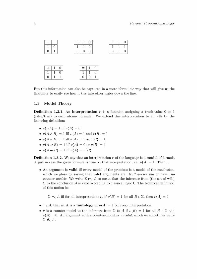
1.2 Truth Tables
The classical theory of meaning of the connectives is captured by the following matrices.
1You may be used to writing the material conditional with the arrow (‘Ñ’) rather than the horseshoe(‘’), and the biconditional with a double arrow (‘Ø’) rather than three lines (‘’). These notations areequivalent, but we will reserve the horseshoe for the truth-conditional, material conditional.
3
4 Review: Propositional Logic
1 00 1
^ 1 0
1 1 00 0 0
_ 1 0
1 1 10 1 0
1 0
1 1 00 1 1
1 0
1 1 00 0 1
But this information can also be captured in a more ‘formulaic way that will give us theflexibility to easily see how it ties into other logics down the line.
1.3 Model Theory
Definition 1.3.1. An interpretation ν is a function assigning a truth-value 0 or 1(false/true) to each atomic formula. We extend this interpretation to all wffs by thefollowing definition:
• νp Aq = 1 iff νpAq = 0
• νpA^Bq = 1 iff νpAq = 1 and νpBq = 1
• νpA_Bq = 1 iff νpAq = 1 or νpBq = 1
• νpA Bq = 1 iff νpAq = 0 or νpBq = 1
• νpA Bq = 1 iff νpAq = νpBq
Definition 1.3.2. We say that an interpretation ν of the language is a model of formulaA just in case the given formula is true on that interpretation, i.e. νpAq = 1. Then . . .
• An argument is valid iff every model of the premises is a model of the conclusion,which we gloss by saying that valid arguments are truth-preserving or have nocounter-models. We write Σ (C A to mean that the inference from (the set of wffs)Σ to the conclusion A is valid according to classical logic C. The technical definitionof this notion is:
Σ (C A iff for all interpretations ν, if νpBq = 1 for all B P Σ, then νpAq = 1.
• (C A, that is, A is a tautology iff νpAq = 1 on every interpretation.
• ν is a counter-model to the inference from Σ to A if νpBq = 1 for all B P Σ andνpAq = 0. An argument with a counter-model is invalid, which we sometimes writeΣ *C A.
1.4 Tableaux 5
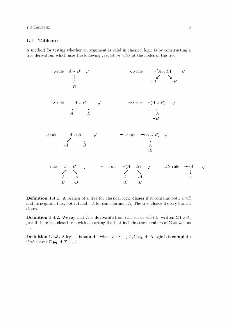
1.4 Tableaux
A method for testing whether an argument is valid in classical logic is by constructing atree derivation, which uses the following resolution rules at the nodes of the tree.
^-rule A^B`
^-rule pA^Bq`
Ó Ö ×A A BB
_-rule A_B`
_-rule pA_Bq`
Ö × ÓA B A
B
-rule A B`
-rule pA Bq`
Ö × Ó A B A
B
-rule A B`
-rule pA Bq`
DN-rule A`
Ö × Ö × ÓA A A A AB B B B
Definition 1.4.1. A branch of a tree for classical logic closes if it contains both a wffand its negation (i.e., both A and A for some formula A) The tree closes if every branchcloses.
Definition 1.4.2. We say that A is derivable from (the set of wffs) Σ, written Σ $C A,just if there is a closed tree with a starting list that includes the members of Σ as well as A.
Definition 1.4.3. A logic L is sound if whenever Σ $L A,Σ (L A. A logic L is completeif whenever Σ (L A,Σ $L A.
6 Review: Propositional Logic
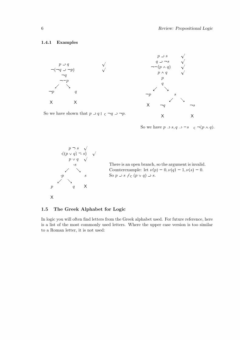
1.4.1 Examples
p q`
p q pq`
q p
Ö × p q
X X
So we have shown that p q $C q p.
p s`
q s`
pp^ qq`
p^ q`
pq
Ö × p s
Ö ×X q s
X X
So we have p s, q s $C pp^ qq.
p s`
ppp_ qq sq`
p_ q`
sÖ ×
p sÖ ×
p q X
X
There is an open branch, so the argument is invalid.Counterexample: let νppq 0, νpqq 1, νpsq 0.So p s &C pp_ qq s.
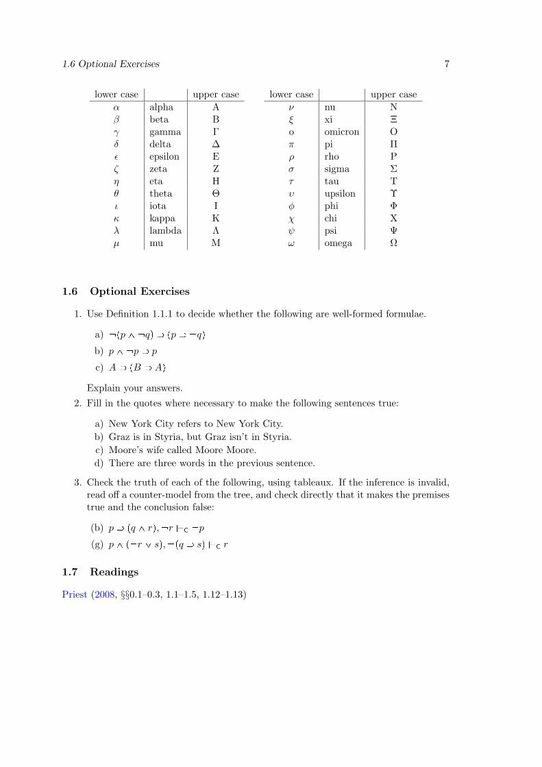
1.5 The Greek Alphabet for Logic
In logic you will often find letters from the Greek alphabet used. For future reference, hereis a list of the most commonly used letters. Where the upper case version is too similarto a Roman letter, it is not used:
1.6 Optional Exercises 7
lower case upper case
α alpha Aβ beta Bγ gamma Γδ delta ∆ϵ epsilon Eζ zeta Zη eta Hθ theta Θι iota Iκ kappa Kλ lambda Λµ mu M
lower case upper case
ν nu Nξ xi Ξo omicron Oπ pi Πρ rho Pσ sigma Στ tau Tυ upsilon Υϕ phi Φχ chi Xψ psi Ψω omega Ω
1.6 Optional Exercises
1. Use Definition 1.1.1 to decide whether the following are well-formed formulae.
a) pp^ qq pp qq
b) p^ p p
c) A pB Aq
Explain your answers.
2. Fill in the quotes where necessary to make the following sentences true:
a) New York City refers to New York City.
b) Graz is in Styria, but Graz isn’t in Styria.
c) Moore’s wife called Moore Moore.
d) There are three words in the previous sentence.
3. Check the truth of each of the following, using tableaux. If the inference is invalid,read off a counter-model from the tree, and check directly that it makes the premisestrue and the conclusion false:
(b) p pq ^ rq, r $C p
(g) p^ p r _ sq, pq sq $C r
1.7 Readings
Priest (2008, §§0.1–0.3, 1.1–1.5, 1.12–1.13)

2 Review: Predicate Logic
2.1 Language
Definition 2.1.1. The basic vocabulary of the language of first-order logic (or predicatelogic) L includes:
• individual variables x, y, z, with or without numerical subscripts
• individual constants a, b, c, with or without numerical subscripts
• for every natural number n ¿ 0, n-place predicates Pn, Qn, Sn, with or withoutnumerical subscripts1
• unary connective and binary connectives ^,_,,
• quantifiers @ and D
• parentheses p, q
We will call any individual variable or constant a term.
Definition 2.1.2. A well-formed formula, or wff, of first-order logic is defined asfollows:
• if Π is any n-place predicate and t1, . . . , tn are any terms, then Πt1 . . . tn is an atomicwff
• if A and B are wffs, so are A, pA^Bq, pA_Bq, pA Bq, pA Bq
• if A is any wff and α is any variable, then @αA, DαA are wffs
• nothing else is a wff.
Definition 2.1.3. An occurrence of a variable α in wff A is bound in A if that occurrenceis within an occurrence of some wff of the form @αB or DαB within A. Otherwise theoccurrence is free in A.A formulae with no free occurrences of variables is said to be closed; otherwise it is open.Apαβq is the formula obtained by substituting β for each free occurrence of α in A.
1We may occasionally leave out the subscripts when the adicity of the predicate is obvious from thecontext.
9
10 Review: Predicate Logic
2.2 Model Theory
Definition 2.2.1. A model M for PL is an ordered pair xD,J y such that:
• D is a non-empty set (the domain, or universe)
• J is a function (the interpretation function) obeying the following constraints:
– if t is an individual constant then J ptq P D– if Π is an n-place predicate, then J pΠq is an n-place relation over D
Definition 2.2.2. g is a variable assignment for model xD,J y iff g is a function thatassigns to each variable some object in D.gαd is the variable assignment that is just like g, except that it assigns d to α, where d issome object in D. Note that gαdpαq = d.
Definition 2.2.3. Let M (= xD,J y) be a model, g be a variable assignment, and t be aterm. rtsM,g, i.e. the denotation of t (relative to M and g), is defined as follows:
rtsM,g
"J ptq if t is a constantgptq if t is a variable
Definition 2.2.4. The valuation function, νM,g, for model M (= xD,J y) and variableassignment g, is defined as the function that assigns to each wff either 0 or 1 subject tothe following constraints:
(i) for any n-place predicate Π and any terms t1 . . . tn, νM,gpΠt1 . . . tnq= 1 iff xrt1sM,g . . . rtnsM,gy PJ pΠq.
(ii) For any wffs A,B and any variable α:
νM,gp Aq = 1 iff νM,gpAq = 0νM,gpA^Bq = 1 iff νM,gpAq = 1 and νM,gpBq = 1νM,gpA_Bq = 1 iff νM,gpAq = 1 or νM,gpBq = 1νM,gpA Bq = 1 iff νM,gpAq = 0 or νM,gpBq = 1νM,gpA Bq = 1 iff νM,gpAq = νM,gpBqνM,gp@αAq = 1 iff for every d P D, νM,gαdpAq = 1
νM,gpDαAq = 1 iff for at least one d P D, νM,gαdpAq = 1
Read ‘νM,gpAq = 1’ as A is true in (model) M relative to (variable assignment) g.
Definition 2.2.5. A is true in model M iff νM,gpAq = 1, for each variable assignmentg for M.
Definition 2.2.6. The inference from (the set of wffs) Σ to the conclusion A is validaccording to predicate logic PL (Σ (PL A) iff for every model M and every variableassignment g for M , if νM,gpBq = 1 for each B P Σ, then νM,gpAq = 1.When Σ (PL A, we also say that A is a semantic consequence in PL of the set of wffsΣ.A wff A is valid in PL ((PL A) iff A is true in all models for PL.
2.3 Tableaux 11
2.3 Tableaux
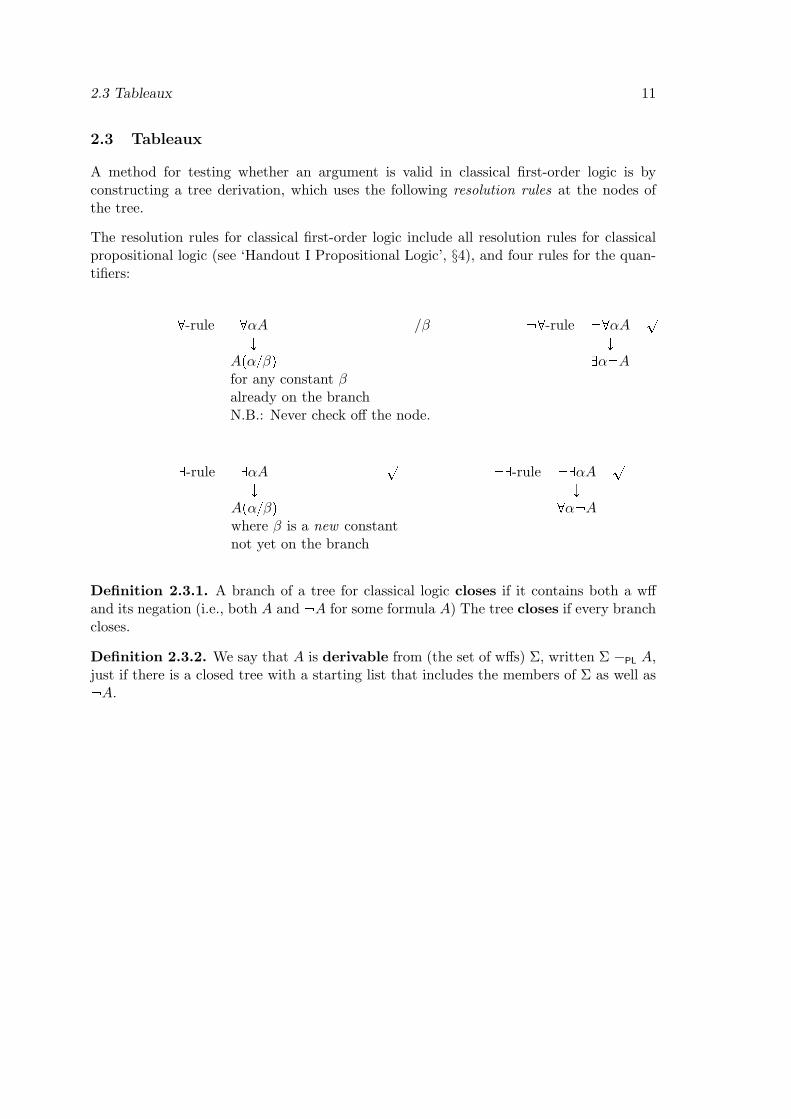
A method for testing whether an argument is valid in classical first-order logic is byconstructing a tree derivation, which uses the following resolution rules at the nodes ofthe tree.
The resolution rules for classical first-order logic include all resolution rules for classicalpropositional logic (see ‘Handout I Propositional Logic’, §4), and four rules for the quan-tifiers:
@-rule @αA /β @-rule @αA`
Ó ÓApαβq Dα Afor any constant βalready on the branchN.B.: Never check off the node.
D-rule DαA`
D-rule DαA`
Ó ÓApαβq @α Awhere β is a new constantnot yet on the branch
Definition 2.3.1. A branch of a tree for classical logic closes if it contains both a wffand its negation (i.e., both A and A for some formula A) The tree closes if every branchcloses.
Definition 2.3.2. We say that A is derivable from (the set of wffs) Σ, written Σ $PL A,just if there is a closed tree with a starting list that includes the members of Σ as well as A.
12 Review: Predicate Logic
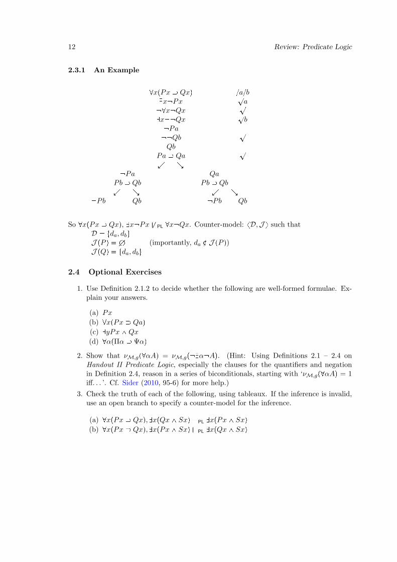
2.3.1 An Example
@xpPx Qxq abDx Px
`a
@x Qx`
Dx Qx`b
Pa Qb
`Qb
Pa Qa`
Ö × Pa Qa
Pb Qb Pb QbÖ × Ö ×
Pb Qb Pb Qb
So @xpPx Qxq, Dx Px &PL @x Qx. Counter-model: xD,J y such thatD tda, dbuJ pP q H (importantly, da R J pP q)J pQq tda, dbu
2.4 Optional Exercises
1. Use Definition 2.1.2 to decide whether the following are well-formed formulae. Ex-plain your answers.
(a) Px
(b) @xpPx Qaq
(c) DyPx^Qx
(d) @αpΠα Ψαq
2. Show that νM,gp@αAq = νM,gp Dα Aq. (Hint: Using Definitions 2.1 – 2.4 onHandout II Predicate Logic, especially the clauses for the quantifiers and negationin Definition 2.4, reason in a series of biconditionals, starting with ‘νM,gp@αAq = 1iff. . . ’. Cf. Sider (2010, 95-6) for more help.)
3. Check the truth of each of the following, using tableaux. If the inference is invalid,use an open branch to specify a counter-model for the inference.
(a) @xpPx Qxq, DxpQx^ Sxq $PL DxpPx^ Sxq
(b) @xpPx Qxq, DxpPx^ Sxq $PL DxpQx^ Sxq

2.5 Readings 13
2.5 Readings
Obligatory reading: Priest (2008, ch. 12)
Optional readings: Sider (2010, §§4.1–4.3), Bell et al. (2001, §§2.1–2.3, 2.5–2.6)

3 Set Theory Tutorial
3.1 Sets
The basic intuition of set theory is that one can group objects together into a collection orset, in such a way that, presented with an object, u, and such a set, A, one can sensiblyask whether the object belongs to, or is a member of, the set. The basic relation issymbolised by
u P A
If u is not a member of A, we write
u R A
A set is determined by its members:
Definition 3.1.1. The intuitive principle of extension. Two sets are equal iff theyhave the same members. We write ‘A B’ iff A and B are equal, and ‘A B’ iff A andB are inequal.
We can write sets by simply listing its members between curly brackets. Thus, 2,4, 6 = 2, 6, 4. Sets may be infinite, which we can write, e.g. in the following way: 1, 2, 3, . . . . Another way to give a set is by specifying the (necessary and sufficient)condition(s) for membership in the set:
Definition 3.1.2. The intuitive principle of abstraction. A formula P pxq defines aset A by the convention that the members of A are exactly those objects a such that P paqis true. We write: A = tx|P pxqu.
Example: ty|y is divisible by 2
txu, a unit set or singleton set, is the set whose sole member is x. The set with nomembers is the empty set, H; that is, for every object u, u is not a member ofH (u R H).
15
16 Set Theory Tutorial
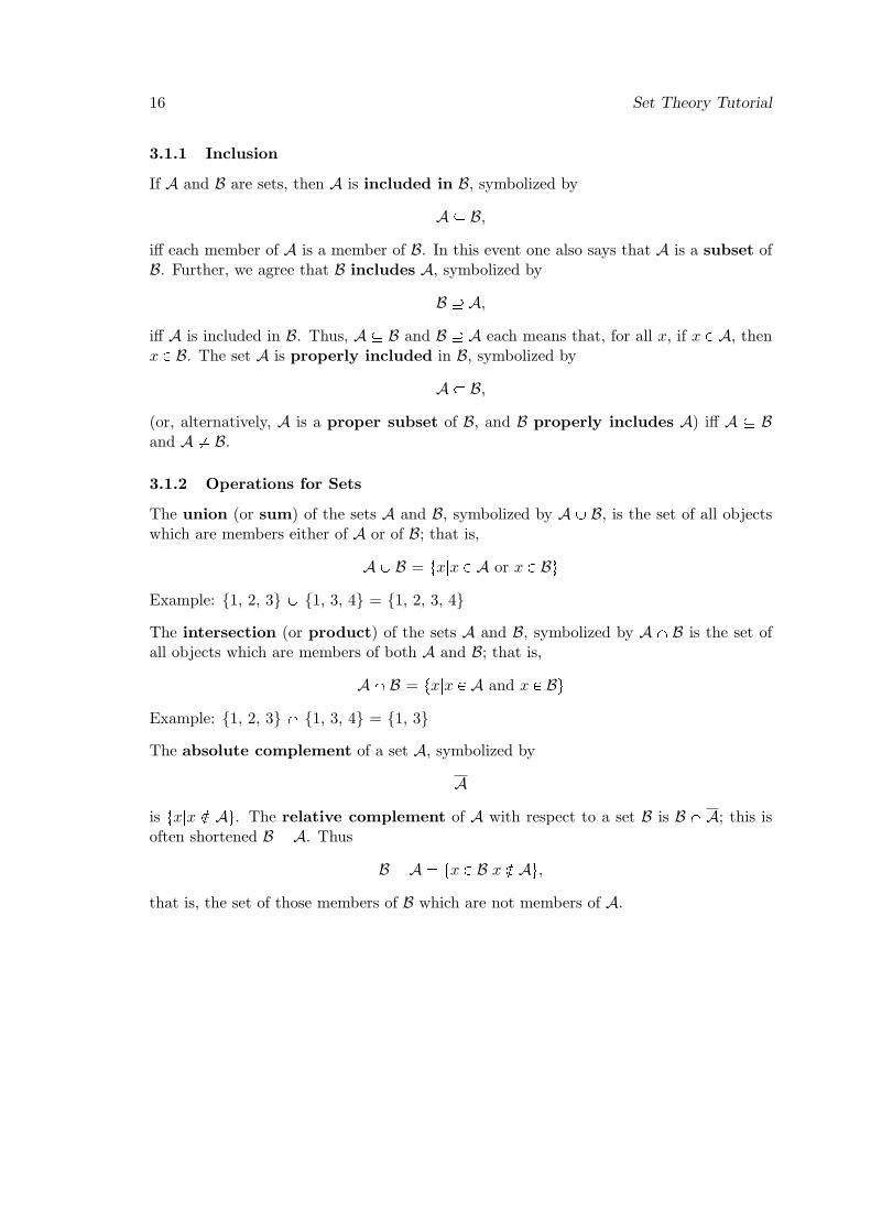
3.1.1 Inclusion
If A and B are sets, then A is included in B, symbolized by
A B,
iff each member of A is a member of B. In this event one also says that A is a subset ofB. Further, we agree that B includes A, symbolized by
B A,
iff A is included in B. Thus, A B and B A each means that, for all x, if x P A, thenx P B. The set A is properly included in B, symbolized by
A B,
(or, alternatively, A is a proper subset of B, and B properly includes A) iff A Band A B.
3.1.2 Operations for Sets
The union (or sum) of the sets A and B, symbolized by A Y B, is the set of all objectswhich are members either of A or of B; that is,
AY B = tx|x P A or x P Bu
Example: 1, 2, 3 Y 1, 3, 4 = 1, 2, 3, 4
The intersection (or product) of the sets A and B, symbolized by A X B is the set ofall objects which are members of both A and B; that is,
AX B = tx|x P A and x P Bu
Example: 1, 2, 3 X 1, 3, 4 = 1, 3
The absolute complement of a set A, symbolized by
A
is tx|x R Au. The relative complement of A with respect to a set B is B X A; this isoften shortened B A. Thus
B A tx P B|x R Au,
that is, the set of those members of B which are not members of A.
3.2 Relations 17
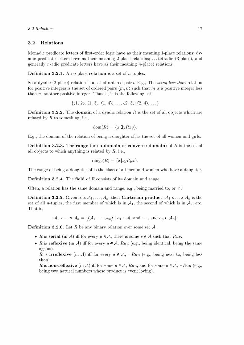
3.2 Relations
Monadic predicate letters of first-order logic have as their meaning 1-place relations; dy-adic predicate letters have as their meaning 2-place relations; . . . tetradic (3-place), andgenerally n-adic predicate letters have as their meaning n-place) relations.
Definition 3.2.1. An n-place relation is a set of n-tuples.
So a dyadic (2-place) relation is a set of ordered pairs. E.g., The being less-than relationfor positive integers is the set of ordered pairs xm,ny such that m is a positive integer lessthan n, another positive integer. That is, it is the following set:
x1, 2y, x1, 3y, x1, 4y, . . . , x2, 3y, x2, 4y, . . .
Definition 3.2.2. The domain of a dyadic relation R is the set of all objects which arerelated by R to something, i.e.,
dom(R) = x|DyRxy.
E.g., the domain of the relation of being a daughter of, is the set of all women and girls.
Definition 3.2.3. The range (or co-domain or converse domain) of R is the set ofall objects to which anything is related by R, i.e.,
range(R) = x|DyRyx.
The range of being a daughter of is the class of all men and women who have a daughter.
Definition 3.2.4. The field of R consists of its domain and range.
Often, a relation has the same domain and range, e.g., being married to, or ¤.
Definition 3.2.5. Given sets A1, . . . ,An, their Cartesian product, A1 x . . . x An is theset of all n-tuples, the first member of which is in A1, the second of which is in A2, etc.That is,
A1 x . . . x An = txA1, . . . ,Any | a1 P A1,and . . . , and an P Anu
Definition 3.2.6. Let R be any binary relation over some set A.
• R is serial (in A) iff for every u P A, there is some v P A such that Ruv.
• R is reflexive (in A) iff for every u P A, Ruu (e.g., being identical, being the sameage as).R is irreflexive (in A) iff for every u P A, Ruu (e.g., being next to, being lessthan).R is non-reflexive (in A) iff for some u P A, Ruu, and for some u P A, Ruu (e.g.,being two natural numbers whose product is even; loving).
18 Set Theory Tutorial
• R is symmetric iff for all u, v, if Ruv then Rvu (e.g., being identical, being adjacentto).R is asymmetric iff for all u, v, if Ruv then Rvu (e.g., being less than).R is anti-symmetric iff for all u, v, if Ruv and u v then Rvu (e.g., being lessthan or equal to).R is non-symmetric iff for some u, v, Ruv and Rvu, and for some u, v Ruv andRvu (e.g., liking).
• R is transitive iff for any u, v, w, if Ruv and Rvw then Ruw (e.g., identity, beingless than, being less than or equal to).R is intransitive iff for any u, v, w, if Ruv and Rvw then Ruw (e.g., being thesquare of (on the positive integers ¥2)).R is non-transitive iff for some u, v, w, if Ruv and Rvw then Ruw, and for someu, v, w, if Ruv and Rvw then Ruw (e.g., being similar, liking).
• R is an equivalence relation (in A) iff R is symmetric, transitive, and reflexive(in A) (e.g., being equal to (in A=N), having the same birthday as (in A = the setof all people)).
3.3 Functions
Definition 3.3.1. A function is a set of ordered pairs, f , obeying the condition that ifxu, vy and xu,wy are both members of f , then v w.When xu, vy P f , we say that u is an argument of f , v is a value of f , and that f mapsu to v; we write ‘fpuq v.’ The domain of a function is the set of its arguments, itsrange is the set of its values. A function is n-place when every member of its domain isan n-tuple.
A function is a binary relation that never relates a single argument to two distinct values.A function is called one-to-one if it maps distinct elements to distinct elements; i.e., afunction f is one-to-one iff u v implies fpuq fpvq. For instance, fpxq 2x 1 (in N)is one-to-one.
3.4 Readings
Obligatory reading: Priest (2008, §§01.–0.3)
Optional reading: Sider (2010, pp. 12–16)

Part II
Modality
19

4 Propositional Modal Logic
4.1 Motivating Modal Semantics
• Modal logic is narrowly defined as the logic of necessity and possibility: it is necessarythat. . . & it it is possible that. . .
• It concerns two modes in which propositions (more generally, any truth bearer) canbe true or false.
• The notion of modality (in contemporary linguistics) is much wider: “modality isthe linguistic phenomenon whereby grammar allows one to say things about, or onthe basis of, situations which need not be real.” (Portner, 2009, 1)
• It’s an open research question which features of language are associated with mod-ality. Take for example tense: Are the past and future real? Hence, do past tenseand future tense expressions (-ed, will+verb) have modal meanings?
• Kinds of (English) expressions that have modal meanings (cf. von Fintel (2006))
1. Modal auxiliaries:Sandy must/should/might/may/could be home.
2. Semimodal Verbs:Sandy has to/ought to/needs to be home.
3. Modal adverbs:Perhaps, Sandy is home.
4. Nouns:There is a slight possibility that Sandy is home.
5. Adjectives:It is far from necessary that Sandy is home.
6. Conditionals:If the light is on, Sandy is home.
• Kinds of Modal Meaning:
21
22 Propositional Modal Logic
– Alethic/logical/metaphysical modality is hard to find in natural languagebut matters to philosophy: it concern what is in the widest sense/logically/metaphysicallypossible or necessary.
– Epistemic modality (Greek episteme, meaning ‘knowledge) concerns what ispossible or necessary given what is known and what the available evidence is.
(4.1) A: Where is Paul?B: I don’t know. He may be at home.
– Deontic modality (Greek: deon, meaning ‘duty) concerns what is possible,necessary, permissible, or obligatory, given a body of law or a set of moralprinciples or the like.
(4.2) He may bring his partner to the dinner.
– Bouletic modality concerns what is possible or necessary, given a personsdesires.
(4.3) You should try this cake, given how much you love chocolate.
– Circumstantial modality (sometimes called dynamic modality) concerns whatis possible or necessary, given a particular set of circumstances.
(4.4) Tulips can grow here.
– Teleological modality (Greek telos, meaning ‘goal) concerns what means arepossible or necessary for achieving a particular goal.
(4.5) To get to the Isle of Mull, you must take a ferry.
–...
Why a logic of (different kinds of) necessity and possibility?
(4.6) Durs Grunbein isn’t necessarily going to win a Nobel prize next year.
(4.7) It’s possible that Durs Grunbein will not win a Nobel prize next year.
• It seems that if (4.6) is true, (4.7) has to be true as well.
• This inference relies crucially on the modal adverb necessarily and the sententialmodal operator possible.
Can we just add modal operators to propositional logic?
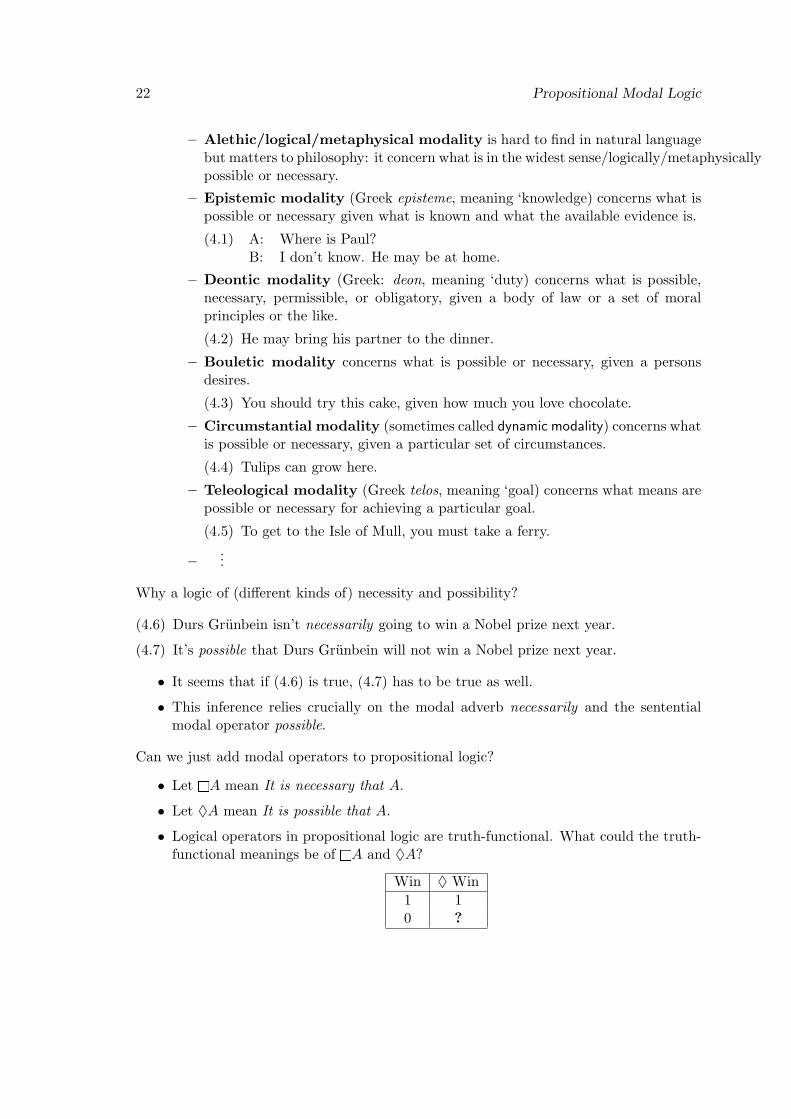
• Let lA mean It is necessary that A.
• Let A mean It is possible that A.
• Logical operators in propositional logic are truth-functional. What could the truth-functional meanings be of lA and A?
Win Win
1 10 ?
4.2 Language 23
• Both choices (0 & 1) get things wrong:
– Its consistent to say that Grunbein didn’t win a Nobel prize, but it was possiblefor him to win one.So 0 is wrong
– Also consistent: Grunbein didn’t win a Nobel prize, and it wasnt even possiblefor him to win it.So 1 is wrong too.
• The truth value of A doesn’t determine the truth value of A.
• Parallel difficulties apply to lA.
• We need more in our semantics than truth-functional propositional operators.
Two important ideas that modal semantics implement:
1. Possible worlds: a possible world can be understood as a way the world mighthave been – a way that the totality of things/events/states of affairs might havebeen. The way things in fact are – the so-called actual world – is also a possibleworld.
2. Relative possibility: what is possible (necessary) given how things are may bedifferent from what is possible given how things could be. For example, given howthings actually are, it is (physically) necessary that the Earth’s standard accelerationdue to gravity is g = 9.80665 m/s2. But in a world in which different laws of physicshold sway, and/r Earth has a different mass, Earth’s standard acceleration could benecessarily different. Thus, what is (physically) possible/necessary relative to oneworld need not be what is (physically) possible/necessary relative to another world.
4.2 Language
Definition 4.2.1. A well-formed formula, or wff, of propositional modal logic is definedas follows:
• lowercase letters p, q, r, s, . . . are atomic formulas
• if A is a wff, so are A, lA, A• if A and B are wffs , so are pA^Bq, pA_Bq, pA Bq, pA Bq
• nothing else is a wff.
4.3 Model Theory
• To define a model we need a bit of extra machinery to help us implement theLeibnizian equivalence: ‘Possibly, φ’ =df. ‘φ is true at some possible world’.
24 Propositional Modal Logic
• In order to fix the range of quantification when we say ‘. . . at some world’ we intro-duce the idea of a relation R (accessibility) and read wRx as ‘x is possible relativeto w’.
Definition 4.3.1. A model M for modal propositional logic is a structure xW,R,J ywhere:
• W is a non-empty set of objects, intuitively understood as possible worlds
• R is an accessibility relation between worlds; i.e. R is a binary relation on W (sothat R W x W). We write ‘w1Rw2’ for ‘w2 is accessible from w1’, or ‘w1 sees w2’,which means intuitively that w2 is possible given/relative to w1.
• J is a function assigning a truth-value to each atomic formula relative to each world.That is, for any propositional letter α, and any w PW,J pα,wq is either 1 or 0. Wewill sometimes equivalently write Jwpαq.
Definition 4.3.2. A frame F is an ordered pair xW,Ry, where W is a non-empty setof objects (possible worlds) and R is an accessibility relation between worlds. A modelxW,R,J y is said to be based on the frame xW,Ry.
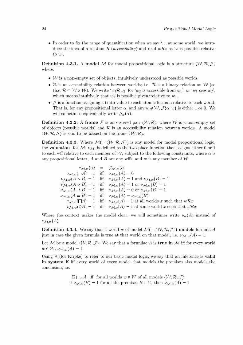
Definition 4.3.3. Where Mp xW,R,J yq is any model for modal propositional logic,the valuation for M, νM, is defined as the two-place function that assigns either 0 or 1to each wff relative to each member of W, subject to the following constraints, where α isany propositional letter, A and B are any wffs, and w is any member of W:
νM,wpαq = JM,wpαqνM,wp Aq 1 iff νM,wpAq 0
νM,wpA^Bq 1 iff νM,wpAq 1 and νM,wpBq 1νM,wpA_Bq 1 iff νM,wpAq 1 or νM,wpBq 1νM,wpA Bq 1 iff νM,wpAq 0 or νM,wpBq 1νM,wpA Bq 1 iff νM,wpAq νM,wpBq
νM,wplAq 1 iff νM,xpAq 1 at all worlds x such that wRxνM,wpAq 1 iff νM,xpAq 1 at some world x such that wRx
Where the context makes the model clear, we will sometimes write νwpAq instead ofνM,wpAq.
Definition 4.3.4. We say that a world w of model Mp xW,R,J yq models formula Ajust in case the given formula is true at that world on that model, i.e. νM,wpAq 1.
Let M be a model xW,R,J y. We say that a formulae A is true in M iff for every worldw PW, νM,wpAq 1.
Using K (for Kripke) to refer to our basic modal logic, we say that an inference is validin system K iff every world of every model that models the premises also models theconclusion; i.e.
Σ (K A iff for all worlds w PW of all models xW,R,J y:if νM,wpBq 1 for all the premises B P Σ, then νM,wpAq 1
4.4 Tableaux 25
When Σ (K A, we also say that A is a semantic consequence in K of the set of wffs Σ.
(K A, that is, A is valid iff νM,wpAq 1 for every world w of every model M.
Model xW,R,J y with world w gives a counter-model to the inference from Σ to A ifνM,wpBq 1 for all B P Σ but νM,wpAq 0. This makes the inference invalid, Σ *K A.
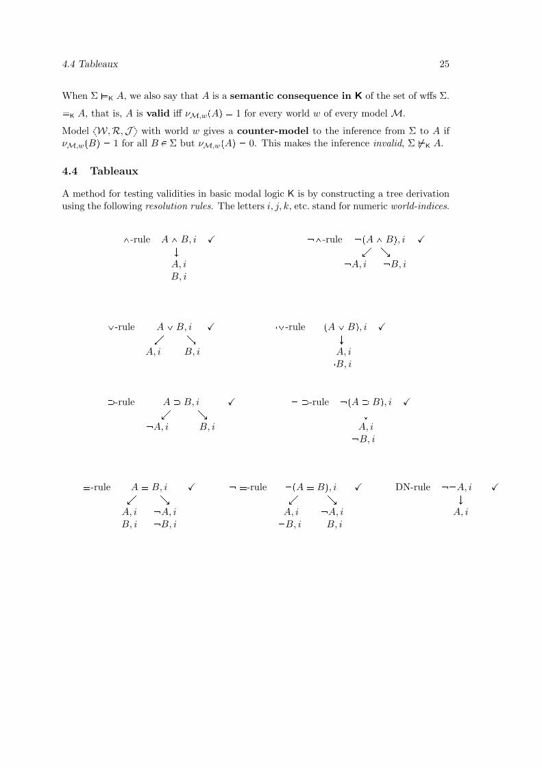
4.4 Tableaux
A method for testing validities in basic modal logic K is by constructing a tree derivationusing the following resolution rules. The letters i, j, k, etc. stand for numeric world-indices.
^-rule A^B, i X ^-rule pA^Bq, i XÓ Ö ×A, i A, i B, iB, i
_-rule A_B, i X _-rule pA_Bq, i XÖ × Ó
A, i B, i A, i B, i
-rule A B, i X -rule pA Bq, i XÖ × Ó
A, i B, i A, i B, i
-rule A B, i X -rule pA Bq, i X DN-rule A, i XÖ × Ö × ÓA, i A, i A, i A, i A, iB, i B, i B, i B, i

26 Propositional Modal Logic
-rule A, i X -rule A, i XÓ Óirj l A, iA, j
using some new index j
l-rule lA, i l-rule lA, i Xirj ÓÓ A, iA, j
for every j such that irj is already on thebranch. N.B. we never check off a l line
An optional, but useful trick is to draw a slash next to a l line. Each time you apply thel-rule write down the index you are applying it to so you know you don’t have to do thatone again.
Definition 4.4.1. A branch of a tree for modal logic closes if it contains a wff and itsnegation with the same world-index (i.e., both A, k and A, k) The tree closes if everybranch does.
Definition 4.4.2. We say that there is a modal tableaux proof from Σ to A, writtenΣ $TK A, just if the tree whose starting list includes B, 0 for each B P Σ as well as A, 0closes.
Definition 4.4.3. We say that there is A is a theorem of K, written $TK A, just if thetree whose starting list includes A, 0 closes.
4.4 Tableaux 27
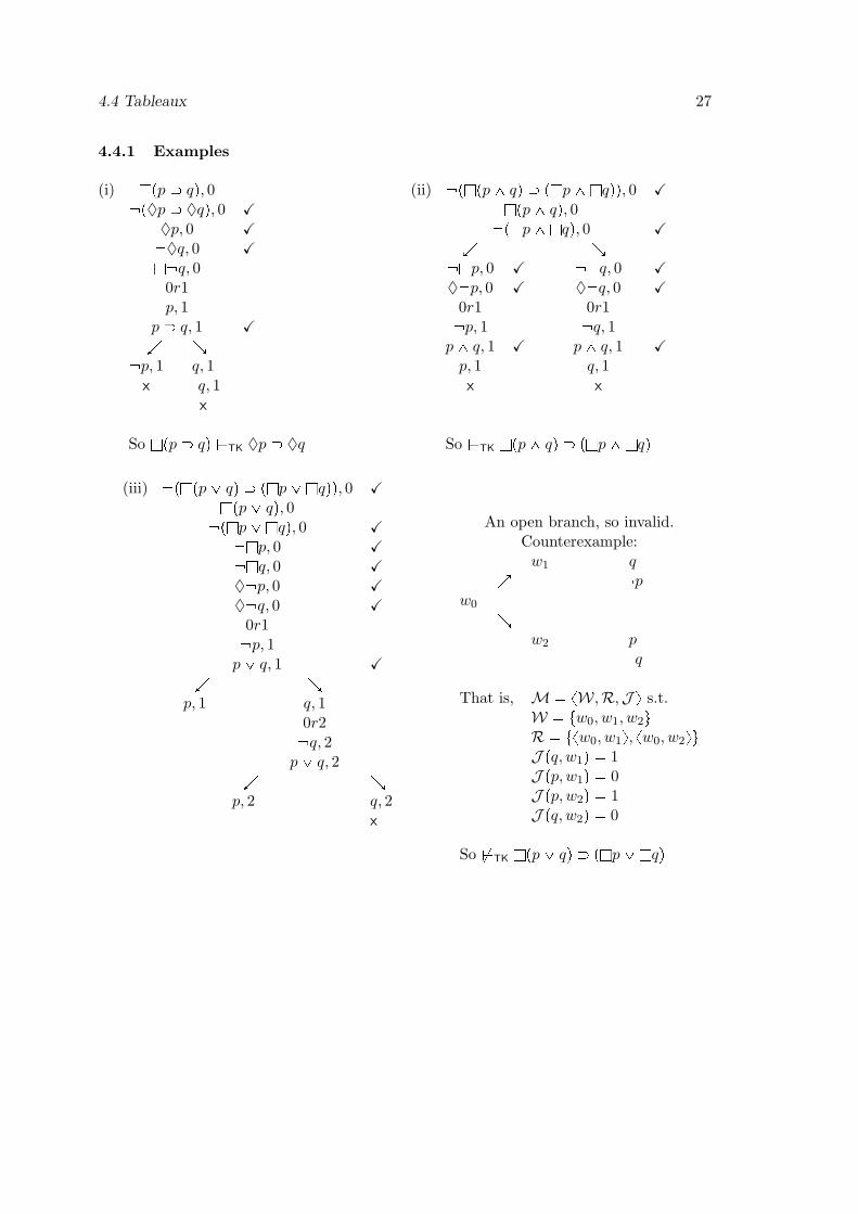
4.4.1 Examples
(i) lpp qq, 0 pp qq, 0 X
p, 0 X q, 0 Xl q, 0
0r1p, 1
p q, 1 XÖ ×
p, 1 q, 1x q, 1
x
So lpp qq $TK p q
(ii) plpp^ qq plp^lqqq, 0 Xlpp^ qq, 0 plp^lqq, 0 X
Ö × lp, 0 X lq, 0 X p, 0 X q, 0 X
0r1 0r1 p, 1 q, 1p^ q, 1 X p^ q, 1 Xp, 1 q, 1x x
So $TK lpp^ qq plp^lqq
(iii) plpp_ qq plp_lqqq, 0 Xlpp_ qq, 0
plp_lqq, 0 X lp, 0 X lq, 0 X p, 0 X q, 0 X
0r1 p, 1p_ q, 1 X
Ö ×p, 1 q, 1
0r2 q, 2p_ q, 2
Ö ×p, 2 q, 2
x
An open branch, so invalid.Counterexample:w1 q
Õ pw0
×w2 p
q
That is, M xW,R,J y s.t.W tw0, w1, w2uR txw0, w1y, xw0, w2yuJ pq, w1q 1J pp, w1q 0J pp, w2q 1J pq, w2q 0
So &TK lpp_ qq plp_lqq
28 Propositional Modal Logic
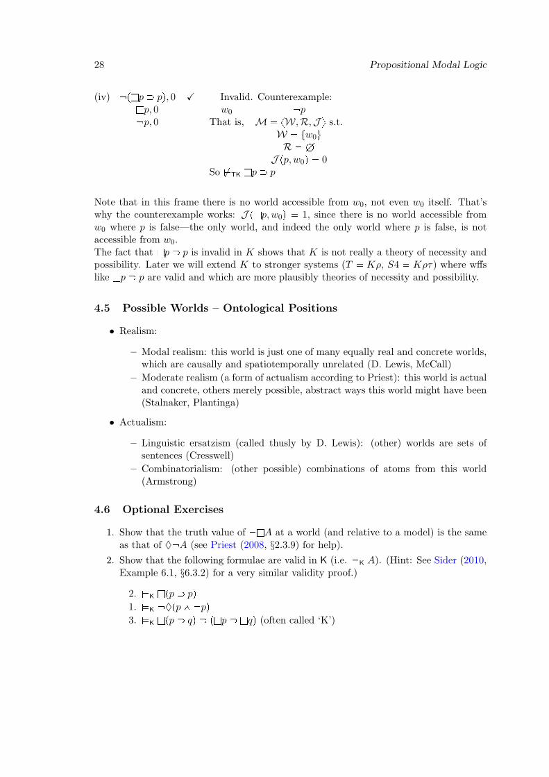
(iv) plp pq, 0 Xlp, 0 p, 0
Invalid. Counterexample:w0 p
That is, M xW,R,J y s.t.W tw0uR H
J pp, w0q 0So &TK lp p
Note that in this frame there is no world accessible from w0, not even w0 itself. That’swhy the counterexample works: J plp, w0q 1, since there is no world accessible fromw0 where p is false—the only world, and indeed the only world where p is false, is notaccessible from w0.The fact that lp p is invalid in K shows that K is not really a theory of necessity andpossibility. Later we will extend K to stronger systems (T Kρ, S4 Kρτ) where wffslike lp p are valid and which are more plausibly theories of necessity and possibility.
4.5 Possible Worlds – Ontological Positions
• Realism:
– Modal realism: this world is just one of many equally real and concrete worlds,which are causally and spatiotemporally unrelated (D. Lewis, McCall)
– Moderate realism (a form of actualism according to Priest): this world is actualand concrete, others merely possible, abstract ways this world might have been(Stalnaker, Plantinga)
• Actualism:
– Linguistic ersatzism (called thusly by D. Lewis): (other) worlds are sets ofsentences (Cresswell)
– Combinatorialism: (other possible) combinations of atoms from this world(Armstrong)
4.6 Optional Exercises
1. Show that the truth value of lA at a world (and relative to a model) is the sameas that of A (see Priest (2008, §2.3.9) for help).
2. Show that the following formulae are valid in K (i.e. (K A). (Hint: See Sider (2010,Example 6.1, §6.3.2) for a very similar validity proof.)
2. (K lpp pq
1. (K pp^ pq3. (K lpp qq plp lqq (often called ‘K’)
4.7 Readings 29
3. Test the following, using tableaux. Where the tableau does not close, use it to definea counter-model, and draw this, as in Priest (2008, §2.4.8).
1. $TK plp^lqq lpp^ qq
2. $TK pp^ qq pp^ qq3. lp,l q $TK lpp qq
4. p,q $TK pp^ qq
4.7 Readings
Obligatory reading: Priest (2008, ch. 2 & §§3.1–3.6)
Optional readings: Sider (2010, §§6.1-6.3); on possible worlds: Read (1994, 96–109)

5 Normal Propositional Modal Logics
5.1 Introduction
• So far, we studied the system K (for Kripke) of propositional modal logic. A char-acteristic theorem of system K is K:
K: lpA Bq plA lBq
• K is plausible enough for necessity: If it’s necessary that B follows from A, thennecessarily B follows from necessarily A.
• Now consider the formula D:
D: lA A• D also seems plausible for necessity: If A is necessary, then it is possible. But D is
not a theorem of K. Is K the right system for necessity?
• There are many systems of modal logics, some of which are more plausibly capturing(a particular kind of) necessity and possibility than others (cf. the kinds of modalmeanings on Handout III-1 ).
• We are looking at some of the more famous ones: normal modal logics D, T, B, S4,S5.
5.2 Normal Systems of Modal Logic
Definition 5.2.1. A system of modal logic, Kn , is a set of premises-conclusion pairs,xΣ, Ay, (where Σ can be H) such that Σ $Kn
A. (Kn is the set of inferences derivable init.) We also call Kn a modal logic.
Definition 5.2.2. A system of modal logic, Kn , is an extension of a system Km just incase if Σ $Km
A, then Σ $KnA. That is, every inference derivable in Km is derivable in
Kn , and every theorem of Km is a theorem of Kn .
Note that by the soundness and completeness of Km and Kn (cf. Handout I, Definition4.3), it also holds that Kn is an extension of Km just in case if Σ (Km
A, then Σ (KnA.
31
32 Normal Propositional Modal Logics
That is, every inference that is valid in Km is valid in Kn , and every logical truth of Km
((KmA) is a logical truth of Kn ; the set of inferences valid in Km (logical truths of Km)
is a subset of the inferences valid in Kn (logical truths in Kn).
When Kn is an extension of Km , we also say that Kn is at least as strong than Km .(When it is a proper extension of Km , we say that it is stronger than Km .)
Definition 5.2.3. A system of modal logic is normal iff it is an extension of K (i.e., iffit is at least as strong as K).
5.2.1 System D (Kη)
• A system stronger than K is D (Priest calls it Kη).
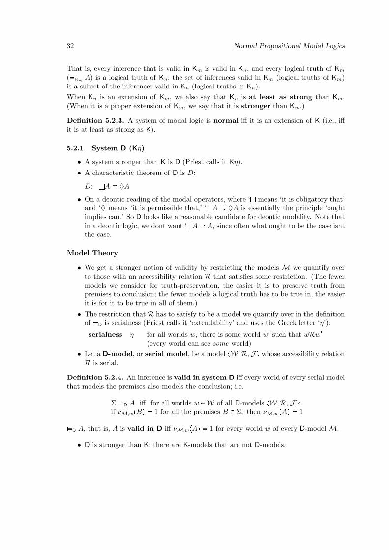
• A characteristic theorem of D is D:
D: lA A• On a deontic reading of the modal operators, where ‘l means ‘it is obligatory that’
and ‘ means ‘it is permissible that,’ ‘lA A is essentially the principle ‘oughtimplies can.’ So D looks like a reasonable candidate for deontic modality. Note thatin a deontic logic, we dont want ‘lA A, since often what ought to be the case isntthe case.
Model Theory
• We get a stronger notion of validity by restricting the models M we quantify overto those with an accessibility relation R that satisfies some restriction. (The fewermodels we consider for truth-preservation, the easier it is to preserve truth frompremises to conclusion; the fewer models a logical truth has to be true in, the easierit is for it to be true in all of them.)
• The restriction that R has to satisfy to be a model we quantify over in the definitionof (D is serialness (Priest calls it ‘extendability’ and uses the Greek letter ‘η’):
serialness η for all worlds w, there is some world w1 such that wRw1(every world can see some world)
• Let a D-model, or serial model, be a model xW,R,J y whose accessibility relationR is serial.
Definition 5.2.4. An inference is valid in system D iff every world of every serial modelthat models the premises also models the conclusion; i.e.
Σ (D A iff for all worlds w PW of all D-models xW,R,J y:if νM,wpBq 1 for all the premises B P Σ, then νM,wpAq 1
(D A, that is, A is valid in D iff νM,wpAq 1 for every world w of every D-model M.
• D is stronger than K: there are K-models that are not D-models.
5.2 Normal Systems of Modal Logic 33
• There are no D-models that are counter-models to D (lA A), but there areK-models that are counter-models to D. (A counter-model to a formula is one inwhich the formula is false.)
Optional Exercise: Find a K-model in which D is false.
Tableaux
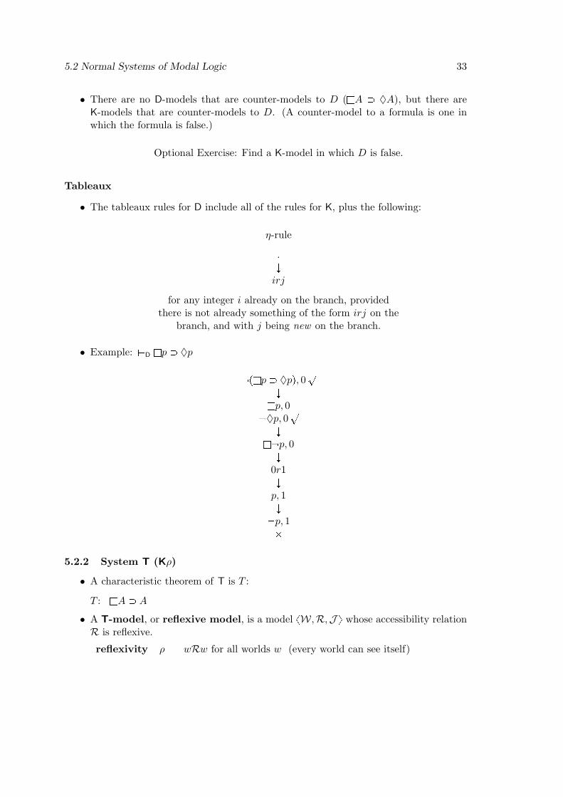
• The tableaux rules for D include all of the rules for K, plus the following:
η-rule
.Óirj
for any integer i already on the branch, providedthere is not already something of the form irj on the
branch, and with j being new on the branch.
• Example: $D lp p
plp pq, 0`Ó
lp, 0 p, 0`
Ól p, 0Ó
0r1Óp, 1Ó
p, 1
5.2.2 System T (Kρ)
• A characteristic theorem of T is T :
T : lA A
• A T-model, or reflexive model, is a model xW,R,J y whose accessibility relationR is reflexive.
reflexivity ρ wRw for all worlds w (every world can see itself)
34 Normal Propositional Modal Logics
Definition 5.2.5. An inference is valid in system T, Σ (T A, iff every world of everyreflexive model that models the premises also models the conclusion. (T A, that is, A isvalid in T iff νM,wpAq 1 for every world w of every T-model M.
• T is stronger than K: there are K-models that are not T-models.
• There are no T-models that are counter-models to T (lA A), but there areK-models that are counter-models to T .
Optional Exercise: Find a D-model in which lA A is false.
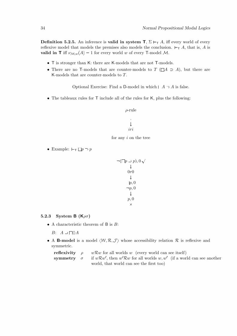
• The tableaux rules for T include all of the rules for K, plus the following:
ρ-rule
.Óiri
for any i on the tree
• Example: $T lp p
plp pq, 0`
Ó0r0Ó
lp, 0 p, 0Óp, 0
5.2.3 System B (Kρσ)
• A characteristic theorem of B is B:
B: A lA• A B-model is a model xW,R,J y whose accessibility relation R is reflexive and
symmetric.
reflexivity ρ wRw for all worlds w (every world can see itself)symmetry σ if wRw1, then w1Rw for all worlds w,w1 (if a world can see another
world, that world can see the first too)
5.2 Normal Systems of Modal Logic 35
Definition 5.2.6. An inference is valid in system B, Σ (B A, iff every world of everyB-model that models the premises also models the conclusion. (B A, that is, A is validin B iff νM,wpAq 1 for every world w of every B-model M.
• B is stronger than K: there are K-models that are not B-models.
• There are no B-models that are counter-models to B (A lA), but there areK-models that are counter-models to B.
Optional Exercise: Find a B-model in which A lA is false.
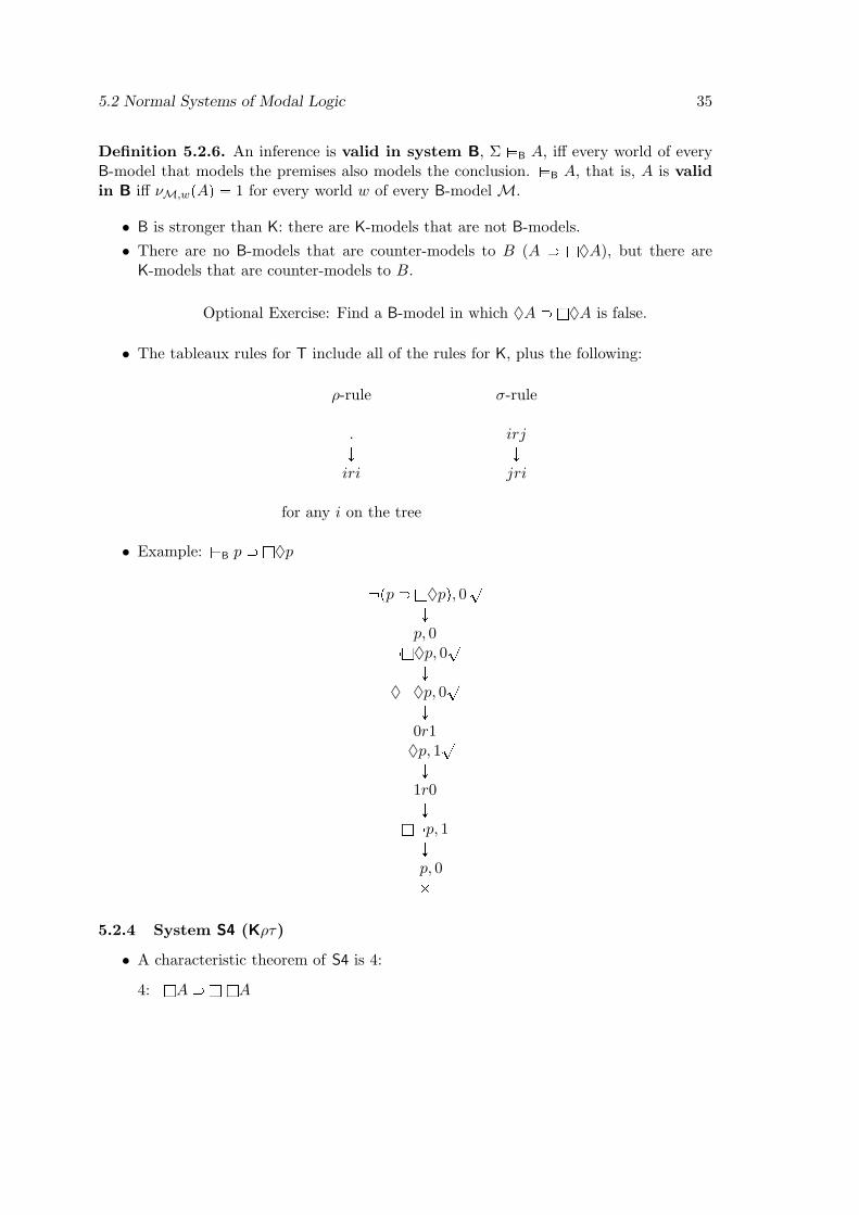
• The tableaux rules for T include all of the rules for K, plus the following:
ρ-rule σ-rule
. irjÓ Óiri jri
for any i on the tree
• Example: $B p lp
pp lpq, 0`Óp, 0
lp, 0`Ó
p, 0`Ó
0r1 p, 1`
Ó1r0Ó
l p, 1Ó
p, 0
5.2.4 System S4 (Kρτ)
• A characteristic theorem of S4 is 4:
4: lA l lA
36 Normal Propositional Modal Logics
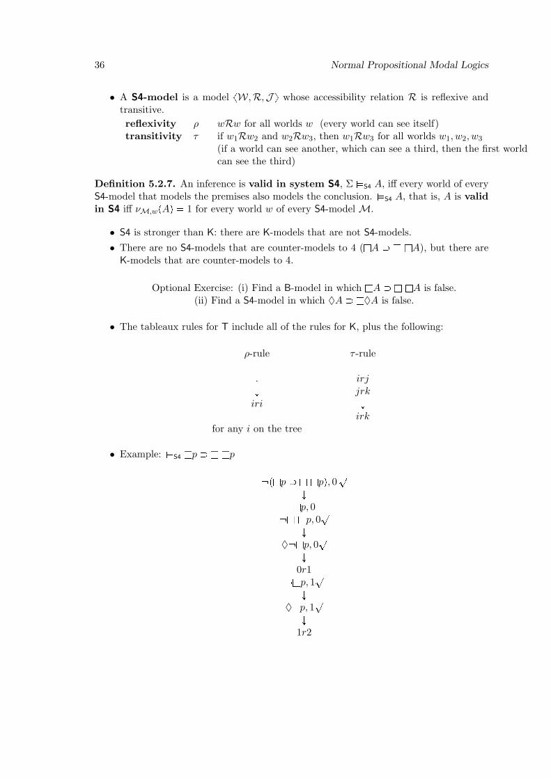
• A S4-model is a model xW,R,J y whose accessibility relation R is reflexive andtransitive.
reflexivity ρ wRw for all worlds w (every world can see itself)transitivity τ if w1Rw2 and w2Rw3, then w1Rw3 for all worlds w1, w2, w3
(if a world can see another, which can see a third, then the first worldcan see the third)
Definition 5.2.7. An inference is valid in system S4, Σ (S4 A, iff every world of everyS4-model that models the premises also models the conclusion. (S4 A, that is, A is validin S4 iff νM,wpAq 1 for every world w of every S4-model M.
• S4 is stronger than K: there are K-models that are not S4-models.
• There are no S4-models that are counter-models to 4 (lA l lA), but there areK-models that are counter-models to 4.
Optional Exercise: (i) Find a B-model in which lA l lA is false.(ii) Find a S4-model in which A lA is false.
• The tableaux rules for T include all of the rules for K, plus the following:
ρ-rule τ -rule
. irjÓ jrkiri Ó
irkfor any i on the tree
• Example: $S4 lp l lp
plp l lpq, 0`
Ólp, 0
l lp, 0`
Ó lp, 0`
Ó0r1
lp, 1`
Ó p, 1`
Ó1r2
5.2 Normal Systems of Modal Logic 37
p, 20r2p, 2
5.2.5 System S5 (Kρστ)
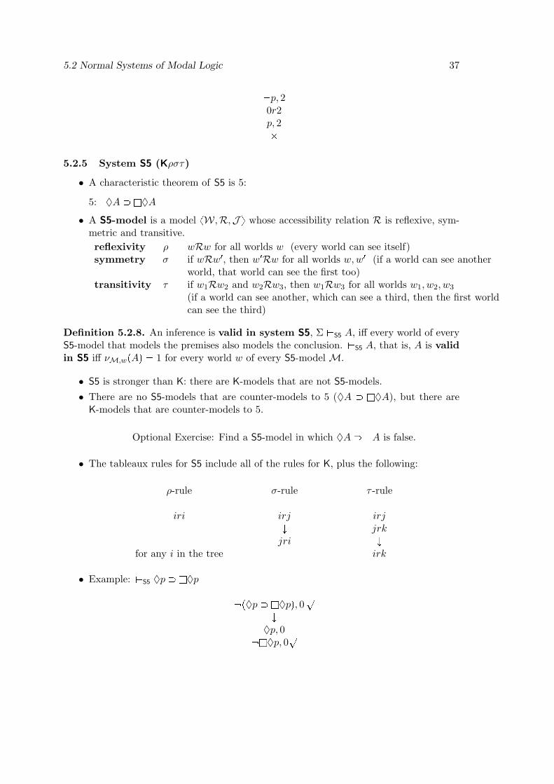
• A characteristic theorem of S5 is 5:
5: A lA• A S5-model is a model xW,R,J y whose accessibility relation R is reflexive, sym-
metric and transitive.
reflexivity ρ wRw for all worlds w (every world can see itself)symmetry σ if wRw1, then w1Rw for all worlds w,w1 (if a world can see another
world, that world can see the first too)transitivity τ if w1Rw2 and w2Rw3, then w1Rw3 for all worlds w1, w2, w3
(if a world can see another, which can see a third, then the first worldcan see the third)
Definition 5.2.8. An inference is valid in system S5, Σ (S5 A, iff every world of everyS5-model that models the premises also models the conclusion. (S5 A, that is, A is validin S5 iff νM,wpAq 1 for every world w of every S5-model M.
• S5 is stronger than K: there are K-models that are not S5-models.
• There are no S5-models that are counter-models to 5 (A lA), but there areK-models that are counter-models to 5.
Optional Exercise: Find a S5-model in which A lA is false.
• The tableaux rules for S5 include all of the rules for K, plus the following:
ρ-rule σ-rule τ -rule
iri irj irjÓ jrkjri Ó
for any i in the tree irk
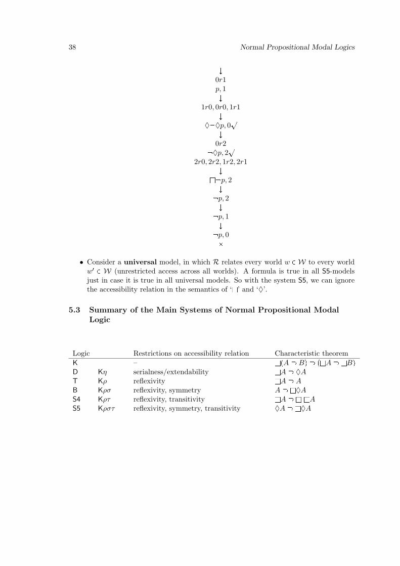
• Example: $S5 p lp
pp lpq, 0`Ó
p, 0 lp, 0`
38 Normal Propositional Modal Logics
Ó0r1p, 1Ó
1r0, 0r0, 1r1Ó
p, 0`Ó
0r2 p, 2`
2r0, 2r2, 1r2, 2r1Ó
l p, 2Ó
p, 2Ó
p, 1Ó
p, 0
• Consider a universal model, in which R relates every world w PW to every worldw1 P W (unrestricted access across all worlds). A formula is true in all S5-modelsjust in case it is true in all universal models. So with the system S5, we can ignorethe accessibility relation in the semantics of ‘l’ and ‘’.
5.3 Summary of the Main Systems of Normal Propositional ModalLogic
Logic Restrictions on accessibility relation Characteristic theorem
K – lpA Bq plA lBqD Kη serialness/extendability lA AT Kρ reflexivity lA AB Kρσ reflexivity, symmetry A lAS4 Kρτ reflexivity, transitivity lA l lAS5 Kρστ reflexivity, symmetry, transitivity A lA
5.4 Optional Exercises 39
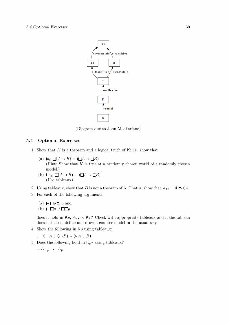
(Diagram due to John MacFarlane)
5.4 Optional Exercises
1. Show that K is a theorem and a logical truth of K; i.e. show that
(a) (K lpA Bq plA lBq(Hint: Show that K is true at a randomly chosen world of a randomly chosenmodel.)
(b) $TK lpA Bq plA lBq(Use tableaux)
2. Using tableaux, show thatD is not a theorem of K. That is, show that&TK lA A.
3. For each of the following arguments
(a) $ lp p and
(b) $ lp llp
does it hold in Kρ, Kσ, or Kτ? Check with appropriate tableaux and if the tableaudoes not close, define and draw a counter-model in the usual way.
4. Show the following in Kρ using tableaux:
$ p A_ Bq _ pA_Bq5. Does the following hold in Kρτ using tableaux?
$ lp lp

40 Normal Propositional Modal Logics
5.5 Readings
Obligatory reading: Priest (2008, §§3.1–3.6)
Optional readings: Sider (2010, §§6.1-6.3)
6 Quantified Modal Logic
6.1 Introduction
Previously, we introduced modal operators by adding possible worlds to our semantics,letting the truth-values of sentences vary relative to each world, and letting the modaloperators ‘look’ across worlds. Interpretations/valuations of propositional logic are basedon the truth-values of atomics, so the basic idea behind possible worlds semantics is toallow any atomic sentence to receive different truth-values at different worlds. Predicatelogic valuations, on the other hand, work differently: they are based on the meaningassigned to terms and predicates. Once these assignments of meaning are settled, thetruth-values of all sentences are settled under that valuation.
We get quantified modal logic, or predicate modal logic, by combining modal logic andpredicate logic: we add bells and whistles to our possible worlds semantics that allowthe meaning assignments of terms and predicates to vary relative to each world and, as aresult, allow the truth-values of sentences to vary relative to each world.
With quantified modal logic, we can — very, very roughly — represent natural languagesentences such as:
‘Necessarily, all musicians play an instrument’: l@xpPx Qxq
‘Some violias could be cellos’: DxpPx^Qxq‘Paul could have been a drummer and Ringo could have been a singer’: Pa^Qb
With the help of quantified modal logic, we can also shed light on a number of philosophicalconcerns about necessity, possibility, essence, and other modal notions. (More on thisbelow)
6.2 Language
Definition 6.2.1. The vocabulary of modal predicate logic, or quantified modal logic,includes the following symbols.
41
42 Quantified Modal Logic
• individual variables x, y, z, with or without numerical subscripts
• individual constants a, b, c, with or without numerical subscripts
• for every natural number n ¿ 0, n-place predicates Pn, Qn, Sn, with or withoutnumerical subscripts
• logical operators: , ^, _, , , l, , @, D• parentheses p, q
Definition 6.2.2. A well-formed formula, or wff, of predicate logic is defined inductively:
• if Π is any n-place predicate and t1, . . . , tn are any terms, then Πt1 . . . tn is an atomicwff
• if A is a wff, so are A, lA, and A• if A and B are wffs, so are pA^Bq, pA_Bq, pA Bq, and pA Bq
• if A is any wff and α is any variable, then @αA, DαA are wffs
• nothing else is a wff.
6.3 Model Theory
The model theory for quantified modal logic combines the model theory of predicate logicwith that of modal logic. (If you’re not sure what the model theory of predicate logiclooks like, have a look at Handout II-1, §2.) We will first look at one way of doing this:constant domain semantics, in which there is just one domain of objects that first-order quantifiers quantify over. On the next handout, we will encounter variable domainsemantics, in which the domain of first-order quantification can vary from possible worldto possible world.
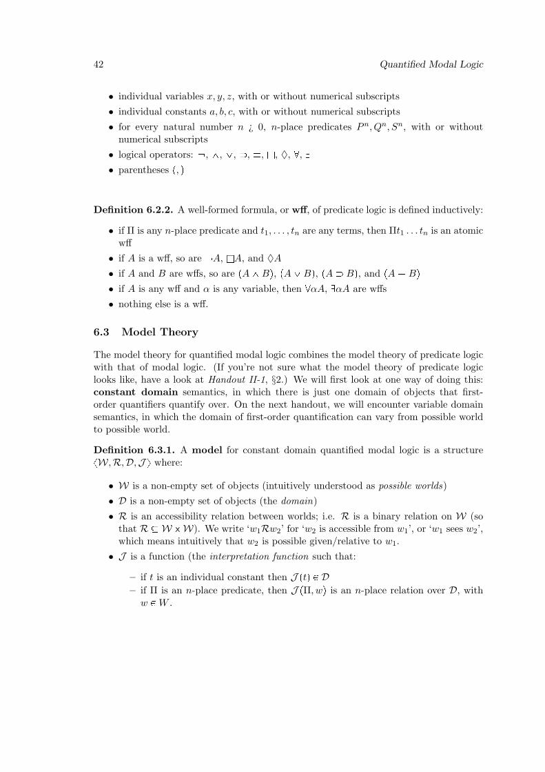
Definition 6.3.1. A model for constant domain quantified modal logic is a structurexW,R,D,J y where:
• W is a non-empty set of objects (intuitively understood as possible worlds)
• D is a non-empty set of objects (the domain)
• R is an accessibility relation between worlds; i.e. R is a binary relation on W (sothat R W x W). We write ‘w1Rw2’ for ‘w2 is accessible from w1’, or ‘w1 sees w2’,which means intuitively that w2 is possible given/relative to w1.
• J is a function (the interpretation function such that:
– if t is an individual constant then J ptq P D– if Π is an n-place predicate, then J pΠ, wq is an n-place relation over D, withw PW .
6.3 Model Theory 43
As before in predicate logic, each constant t is assigned a referent J ptq in the (constant)domain D. So the reference of constants does not vary with possible worlds; a constant hasthe same referent in every possible world. Unlike in standard predicate logic, however, wenow want the properties of objects to vary across worlds, so for each predicate Π and eachworld w, the predicate is given an extension J pΠ, wq relative to that world (an extensionis still a collection of n-place sequences of objects).
The definitions of variable assignment and denotation are almost identical to those forstandard predicate logic (cf. Handout II-1, §2). We do not relativize them to worlds, inthe same way that we do not relativize the referents of constants to worlds.
Definition 6.3.2. g is a variable assignment for model xW,R,D,J y iff g is a functionthat assigns to each variable some object in D.gαd is the variable assignment that is just like g, except that it assigns d to α, where d issome object in D. Note that gαdpαq = d.
Definition 6.3.3. Let M (= xW,R,D,J y) be a model, g be a variable assignment, andt be a term. rtsM,g, i.e. the denotation of t (relative to M and g), is defined as follows:
rtsM,g
"J ptq if t is a constantgptq if t is a variable
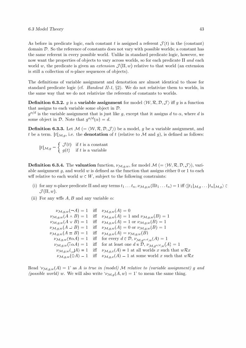
Definition 6.3.4. The valuation function, νM,g,w, for model M (= xW,R,D,J y), vari-able assignment g, and world w is defined as the function that assigns either 0 or 1 to eachwff relative to each world w PW , subject to the following constraints:
(i) for any n-place predicate Π and any terms t1 . . . tn, νM,g,wpΠt1 . . . tnq= 1 iff xrt1sM,g . . . rtnsM,gy PJ pΠ, wq.
(ii) For any wffs A,B and any variable α:
νM,g,wp Aq = 1 iff νM,g,wpAq = 0νM,g,wpA^Bq = 1 iff νM,g,wpAq = 1 and νM,g,wpBq = 1νM,g,wpA_Bq = 1 iff νM,g,wpAq = 1 or νM,g,wpBq = 1νM,g,wpA Bq = 1 iff νM,g,wpAq = 0 or νM,g,wpBq = 1νM,g,wpA Bq = 1 iff νM,g,wpAq = νM,g,wpBqνM,g,wp@αAq = 1 iff for every d P D, νM,gαd,wpAq = 1
νM,g,wpDαAq = 1 iff for at least one d P D, νM,gαd,wpAq = 1
νM,g,wplAq 1 iff νM,g,xpAq 1 at all worlds x such that wRxνM,g,wpAq 1 iff νM,g,xpAq 1 at some world x such that wRx
Read ‘νM,g,wpAq = 1’ as A is true in (model) M relative to (variable assignment) g and(possible world) w. We will also write ‘νM,gpA,wq = 1’ to mean the same thing.
44 Quantified Modal Logic
Definition 6.3.5. Because we are currently dealing with constant domain semantics, wecall our basic quantified modal logic CK or ‘Constant Domain K’.
We say that a world w of model xW,R,D,J y models sentence A iff νM,g,wpAq 1.
An argument is valid in CK iff every world of every model that models the premises alsomodels the conclusion. We write ‘(CK ’ for this semantic consequence relation, and wedefine this notion precisely as follows.
Σ (CK A iff for all worlds w PW of all models xW,R,D,J y and all variable assignments g for M:
if νM,g,wpBq 1 for all the premises B P Σ, then νM,g,wpAq 1
(CK A, that is, A is valid in CK iff νM,g,wpAq 1 for every world w of every model Mand every variable assignment g for M.
Model xW,R,D,J y with world w gives a counter-model to the inference from Σ to A ifνM,g,wpBq 1 for all B P Σ but νM,g,wpAq 0. This makes the inference invalid, *CK A.
Remark. In propositional modal logic, truth-functional connectives are interpreted ‘locally’in the sense that the truth-value at w of a sentence whose main operator is a truth-functional connective is fully determined by the truth-values at w of its parts. In quantifiedmodal logic the quantifiers are also interpreted ‘locally’ in the sense that what determinesthe truth-value of a formula like ‘@xPx’ at world w is just the properties of objects at w.
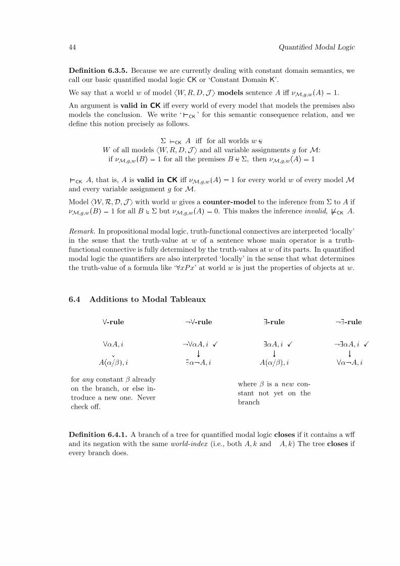
6.4 Additions to Modal Tableaux
@-rule @-rule D-rule D-rule
@αA, i @αA, i X DαA, i X DαA, i XÓ Ó Ó Ó
Apαβq, i Dα A, i Apαβq, i @α A, i
for any constant β alreadyon the branch, or else in-troduce a new one. Nevercheck off.
where β is a new con-stant not yet on thebranch
Definition 6.4.1. A branch of a tree for quantified modal logic closes if it contains a wffand its negation with the same world-index (i.e., both A, k and A, k) The tree closes ifevery branch does.
6.5 The Barcan Formula 45
Definition 6.4.2. We say that there is a modal tableaux proof from Σ to A, writtenΣ $CK A, just in case the tree whose starting list includes B, 0 for each B P Σ as well as A, 0 closes.
Definition 6.4.3. We say that there is A is a theorem of CK, written $CK A, just ifthe tree whose starting list includes A, 0 closes.
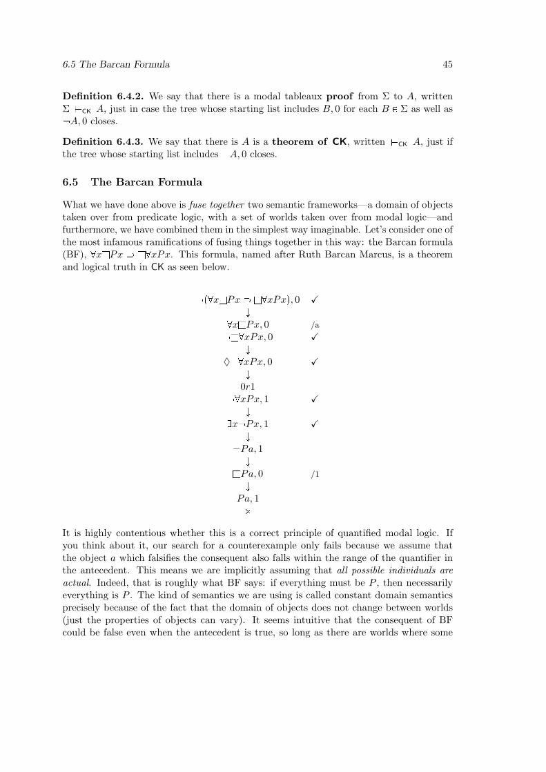
6.5 The Barcan Formula
What we have done above is fuse together two semantic frameworks—a domain of objectstaken over from predicate logic, with a set of worlds taken over from modal logic—andfurthermore, we have combined them in the simplest way imaginable. Let’s consider one ofthe most infamous ramifications of fusing things together in this way: the Barcan formula(BF), @xlPx l@xPx. This formula, named after Ruth Barcan Marcus, is a theoremand logical truth in CK as seen below.
p@xlPx l@xPxq, 0 XÓ
@xlPx, 0 /a
l@xPx, 0 XÓ
@xPx, 0 XÓ
0r1 @xPx, 1 X
ÓDx Px, 1 X
Ó Pa, 1Ó
lPa, 0 /1
ÓPa, 1
It is highly contentious whether this is a correct principle of quantified modal logic. Ifyou think about it, our search for a counterexample only fails because we assume thatthe object a which falsifies the consequent also falls within the range of the quantifier inthe antecedent. This means we are implicitly assuming that all possible individuals areactual. Indeed, that is roughly what BF says: if everything must be P , then necessarilyeverything is P . The kind of semantics we are using is called constant domain semanticsprecisely because of the fact that the domain of objects does not change between worlds(just the properties of objects can vary). It seems intuitive that the consequent of BFcould be false even when the antecedent is true, so long as there are worlds where some
46 Quantified Modal Logic
things exist that do not actually exist. Our semantic framework doesn’t allow this, but ifwe agree that which objects exist should be able to vary between possible worlds, then weshould agree that BF is false.
Consider the formula DxPx DxPx. You can test it to see that it is also a theoremand logical truth, and for the same reasons; it is, in fact, equivalent to BF. The ‘diamond’version makes the criticism especially clear. An instance of this formula, for example, isthe claim that if it is possible that someone jumps nine meters there is someone who canjump nine meters. Or for another instance, if it is possible that there be a Leprechaun,then something exists which could have been a Leprechaun. To many people these soundvery counter-intuitive.
Although this discussion may make it sound obvious how to adjust the semantics to avoidvalidating these formulae, in practice it is complicated. Next week we will discuss analternative approach called ‘variable domain’ semantics, which is an attempt to makegood on our intuition that which objects exist may vary between possible worlds.
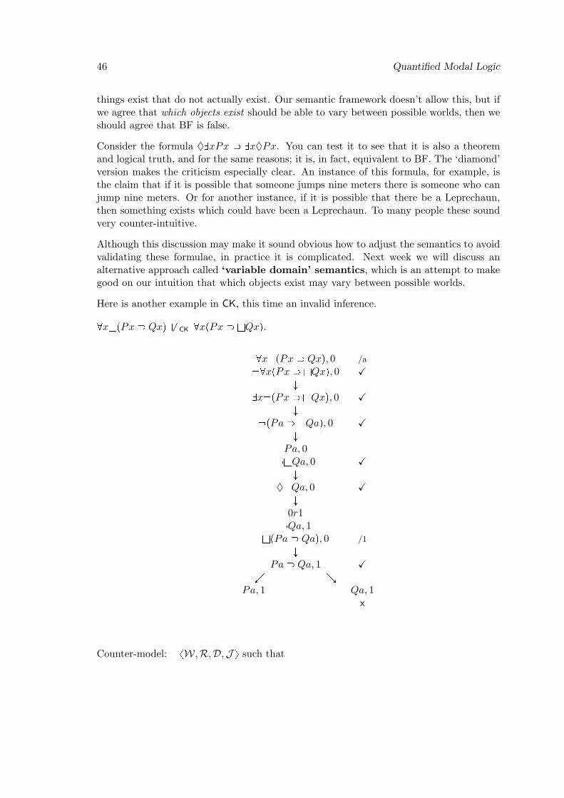
Here is another example in CK, this time an invalid inference.
@xlpPx Qxq &CK @xpPx lQxq.
@xlpPx Qxq, 0 /a
@xpPx lQxq, 0 XÓ
Dx pPx lQxq, 0 XÓ
pPa lQaq, 0 XÓ
Pa, 0 lQa, 0 X
Ó Qa, 0 X
Ó0r1
Qa, 1lpPa Qaq, 0 /1
ÓPa Qa, 1 X
Ö × Pa, 1 Qa, 1
x
Counter-model: xW,R,D,J y such that
6.6 Optional Exercises 47
W tw0, w1uD tδauR txw0, w1yuJ paq δa, J pP,w0q tδau, J pP,w1q H and J pQ,w1q H
6.6 Optional Exercises
1. Test using tableaux. Construct a counter-model if the tree is open.
1. @xlpQx_Hxq $ l@xHx
2. DxlpPx^Qxq $ lDxPx
3. lDxPx $ lDxpPx_Qxq
2. Consider the inference above: @xlpPx Qxq $ @xpPx lQxq
What happens if we add the ρ constraint? Test this using a tree with the ρ rule (cf.Handout III-2, §2.2). Does this have any impact on the result? Does the inferencecome out valid in this system?
6.7 Readings
Obligatory reading: Priest (2008, ch .14)
Optional readings: Sider (2010, §§9.1-9.5); on some philosophical issues: Lowe (2002, pp.79–84)

7 Quantified Modal Logic: Variable Domains
7.1 Constant Domain Quantified Modal Logic
7.1.1 Review
• Model for constant domain Quantified Modal Logic: xW,R,D,J y• This is a very simple way of fusing predicate and modal logic semantics:
A model has a single domain of objects D (hence ‘constant domain’ semantics)
– Quantifiers quantify over the same domain of objects, no matter at which worldwe evaluate a quantified wff for truth
– If ‘Dxpx aq’ is true (false) at some world, it is true (false) at every world.
– Whatever exists at this world exists at every other world.
– Whatever exists at any world exists at this (the actual) world.
7.1.2 Challenges to Constant Domain Quantified Modal Logic
The Barcan Formula
• The Barcan Formula (BF) is a logical truth of CK: (CK @xlPx l@xPx
• Many find it objectionable; an example for materialists:
Everything is necessarily material ÷ Necessarily, everything is material.
@xlMx l@xMx
Everything in our world may be such that it cannot fail to be material. Yet it seemspossible that other things existed which are immaterial.
Necessary Existence
• With a single domain of objects, every object exists at every world. Thus, it existsnecessarily (it cannot fail to exist).
49
50 Quantified Modal Logic: Variable Domains
• But it seems that existence is contingent: I could not have come into existence, thelaptop I’m writing on may not have been manufactured, the cow whose meat you’vehad for dinner last night could have never been conceived, etc.
• But even if it’s a hard metaphysical question whether existence is necessary or con-tingent: Should its answer be a matter of logical truth?
• On constant domain semantics, it is:
(CK @xl Dypy xq(where ‘=’ is a predicate that receives the same interpretation in every model M xW,R,D,J y: J p, wq txd, dy : d P Du)ñ ‘Everything necessarily exists’ is a matter of logical truth.
A Dilemma: What should be in the single domain D?
1. Parsimonious: D contains only really existing things – concrete/spatio-temporal//. . . objectsin the (actual) universe (people, tables, chairs, planets, electrons, . . . )
We take @ and D to have strong ontological import: whatever is in the domainD can truly be said to really exist (not ‘exist’ in some derivative way).
If I want to say that there (really!) are cyclones, I do this as follows: DxCx
Issue 1: (CK @xl Dypy xq
All (concretely/physically/. . . ) things exist necessarily. Issue 2: If we only allow into the domain the objects that actually exist (exist atthe actual world), then we cannot truly say that there could be things that do not(actually) exist: Dxpx aq ^ Dxpx aq
ñ For any a, either it is in the domain (then it also exists at the actual world), orit is not (then it doesn’t exist at any world).
But couldn’t there be things that do not actually exist? Couldn’t there be a son ofL. Wittgenstein?
That is: Someone who doesn’t actually exist but could have existed? (Note that thisis different from someone having the property of possibly being Wittgenstein’s son)
2. Prodigal: In addition to concretely/physically/fundamentally existing things, Dcontains things that exist in some derivative/extraordinary/abstract way (ghosts,golden mountains, talking donkeys, Wittgenstein’s son, . . . )
We do not take @ and D to have strong ontological import: objects in the domaininclude things we do not call ‘existing’ in the strong (concrete) way.
Then we can throw anything in our single domain that we want to say exists at someworld or other: our domain contains Wittgenstein’s son as well as ghosts.
(CK @xl Dypy xq is not so bad: everything exists necessarily in a concreteor abstract way.
7.2 Variable Domain Quantified Modal Logic: Model Theory 51
Issue 1: Hefty metaphysical commitments! Many philosophers consider the postula-tion of such extraordinary things to be obviously false, conceptually incoherent, orworse (cf. the popular criticism of Meinong’s ‘non-existent objects’).
Issue 2: Not clear how we can say that something really exists (at the actual world)(rather than just in this extraordinary way which includes ghosts): ‘Dxpx aq’says only that a exists in a concrete or abstract way
Ways out of the dilemma? (cf. Sider (2010, §9.5); Williamson (1998))
7.1.3 In Defence of Constant Domain Quantified Modal Logic
1. Embrace the first horn (parsimony): Logic is a more reliable guide to (modal) meta-physics than our intuitions about what exists. (Bite the bullet on counter-intuitivecommitments.)
2. Embrace the second horn (prodigality): one big domain of concrete and merelypossible things.
– Express concrete existence by adding a (concrete) existence predicate, E,which at every possible world applies to all and only those things that existconcretely at that world.
– ‘a (concretely) exists’: DxpEx^ x aq
– ‘Everything exists necessarily (concretely)’ is not a logical truth: *CK’ @xl DypEy^y xq
Objections to 2:
1. Hefty metaphysical commitments remain
2. Rendering English into logic is less direct: E must be added to all translationsof sentences expressing concrete existence.
3. The proper role of quantifiers is to record robust ontological commitment (Quine).
7.2 Variable Domain Quantified Modal Logic: Model Theory
• Another way out of the dilemma: Give up the commitment to a single constantdomain
• Make quantification world-relative . . .
• . . . by introducing variable domains into our semantics: a domain for every possibleworld.
• @ and D quantify over different domains, depending on the world at which they arebeing evaluated for truth/falsity.
Definition 7.2.1. A model for variable domain quantified modal logic is a structurexW,R,D,Q,J y where:
52 Quantified Modal Logic: Variable Domains
• W is a non-empty set of objects (intuitively understood as possible worlds)
• R is an accessibility relation between worlds; i.e. R is a binary relation on W (sothat R W x W). We write ‘w1Rw2’ for ‘w2 is accessible from w1’, or ‘w1 sees w2’,which means intuitively that w2 is possible given/relative to w1.
• D is a non-empty set of objects (the super-domain)
• Q is a function that assigns to any w PW a subset of W. We will refer to Qpwq as‘Dw’. Think of Dw as w’s sub-domain — the set of objects that exist at w.
• J is a function (the interpretation function) such that:
– if t is an individual constant then J ptq P D– if Π is an n-place predicate, then J pΠ, wq is an n-place relation over D, withw PW .
Note that D (the super-domain) still includes all possible individuals. But quantifiers @and D range over subsets of D – one for each world w: Dw. When we evaluate a quantifiedsentence such as ‘@xPx1 for truth/falsity, we do so at a world w – and we interpret @xas ranging over w’s subdomain, Dw.
Definition 7.2.2. g is a variable assignment for model xW,R,D,Q,J y iff g is afunction that assigns to each variable some object in D.gαd is the variable assignment that is just like g, except that it assigns d to α, where d issome object in D. Note that gαdpαq = d.
Definition 7.2.3. Let M (= xW,R,D,Q,J y) be a model, g be a variable assignment,and t be a term. rtsM,g, i.e. the denotation of t (relative to M and g), is defined asfollows:
rtsM,g
"J ptq if t is a constantgptq if t is a variable
Definition 7.2.4. The valuation function, νM,g,w, for model M (= xW,R,D,Q,J y),variable assignment g, and world w is defined as the function that assigns either 0 or 1 toeach wff relative to each world w PW , subject to the following constraints:
(i) for any n-place predicate Π and any terms t1 . . . tn, νM,g,wpΠt1 . . . tnq= 1 iff xrt1sM,g . . . rtnsM,gy PJ pΠ, wq.
(ii) For any wffs A,B and any variable α:
7.3 Solving CK’s Issues 53
νM,g,wp Aq = 1 iff νM,g,wpAq = 0νM,g,wpA^Bq = 1 iff νM,g,wpAq = 1 and νM,g,wpBq = 1νM,g,wpA_Bq = 1 iff νM,g,wpAq = 1 or νM,g,wpBq = 1νM,g,wpA Bq = 1 iff νM,g,wpAq = 0 or νM,g,wpBq = 1νM,g,wpA Bq = 1 iff νM,g,wpAq = νM,g,wpBqνM,g,wp@αAq = 1 iff for every d P Dw, νM,gαd,wpAq = 1
νM,g,wpDαAq = 1 iff for at least one d P Dw, νM,gαd,wpAq = 1
νM,g,wplAq 1 iff νM,g,xpAq 1 at all worlds x such that wRxνM,g,wpAq 1 iff νM,g,xpAq 1 at some world x such that wRx
Read ‘νM,g,wpAq = 1’ as A is true in (model) M relative to (variable assignment) g and(possible world) w. We will also write ‘νM,gpA,wq = 1’ to mean the same thing.
Definition 7.2.5. We call our basic quantified modal logic VK or ‘Variable DomainK’.
We say that a world w of model xW,R,D,Q,J y models sentence A iff νM,g,wpAq 1.
An argument is valid in VK iff every world of every model that models the premises alsomodels the conclusion. We write ‘(VK ’ for this semantic consequence relation, and wedefine this notion precisely as follows.
Σ (VK A iff for all worlds w PW of all models xW,R,D,Q,J y and all variable assignments g for M:
if νM,g,wpBq 1 for all the premises B P Σ, then νM,g,wpAq 1
(VK A, that is, A is valid in VK iff νM,g,wpAq 1 for every world w of every model Mand every variable assignment g for M.
Model xW,R,D,Q,J y with world w gives a counter-model to the inference from Σ toA if νM,g,wpBq 1 for all B P Σ but νM,g,wpAq 0. This makes the inference invalid,*VK A.
We get stronger systems of variable domain quantified modal logic by adding constraintson the accessibility relation R — in the same way you do with normal propositional modallogics (e.g. D, T, B, S4, S5) – and defining validity by means of models whose R satisfythe constraint (D-models, T-models, . . . ). Cf. Handout III-2.
7.3 Solving CK’s Issues
• What exists at the actual world @ need not exist at any other world: D@ need notbe a subset of any other w’s domain Dw.
• What exists at some other world w need not exist at the actual world @: D@ neednot be a superset of any other w’s domain Dw.
54 Quantified Modal Logic: Variable Domains
• BF is not valid in VK: *VK @xlPx l@xPx
Take a random world w of model M:
– let the antecedent, ‘@xlPx’, be true at w (given M and g):all d P Dw satisfy P at every world that w accesses.
– the consequent, ‘l@xPx’, can still be false:there may be a world w1 (accessible from w) whose domain Dw1 contains atleast one object d1 not in Dw, which does not satisfy P , so ‘@xPx’ isfalse at w1 and thus ‘l@xPx’ is false.
• No necessary existence: *VK @xl Dypy xq
The formula is false at a world w if w accesses some world w1 whose domain Dw1
fails to contain at least one object d1 that Dw contains.
7.4 Tableaux
7.4.1 A Complication
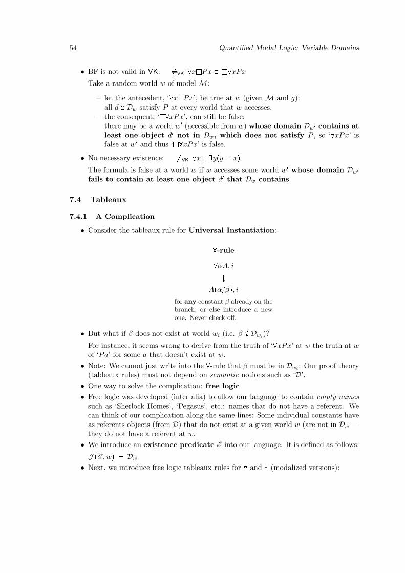
• Consider the tableaux rule for Universal Instantiation:
@-rule
@αA, i
Ó
Apαβq, i
for any constant β already on thebranch, or else introduce a newone. Never check off.
• But what if β does not exist at world wi (i.e. β R Dwi)?
For instance, it seems wrong to derive from the truth of ‘@xPx’ at w the truth at wof ‘Pa’ for some a that doesn’t exist at w.
• Note: We cannot just write into the @-rule that β must be in Dwi : Our proof theory(tableaux rules) must not depend on semantic notions such as ‘D’.
• One way to solve the complication: free logic
• Free logic was developed (inter alia) to allow our language to contain empty namessuch as ‘Sherlock Homes’, ‘Pegasus’, etc.: names that do not have a referent. Wecan think of our complication along the same lines: Some individual constants haveas referents objects (from D) that do not exist at a given world w (are not in Dw —they do not have a referent at w.
• We introduce an existence predicate E into our language. It is defined as follows:
J pE , wq Dw
• Next, we introduce free logic tableaux rules for @ and D (modalized versions):
7.4 Tableaux 55
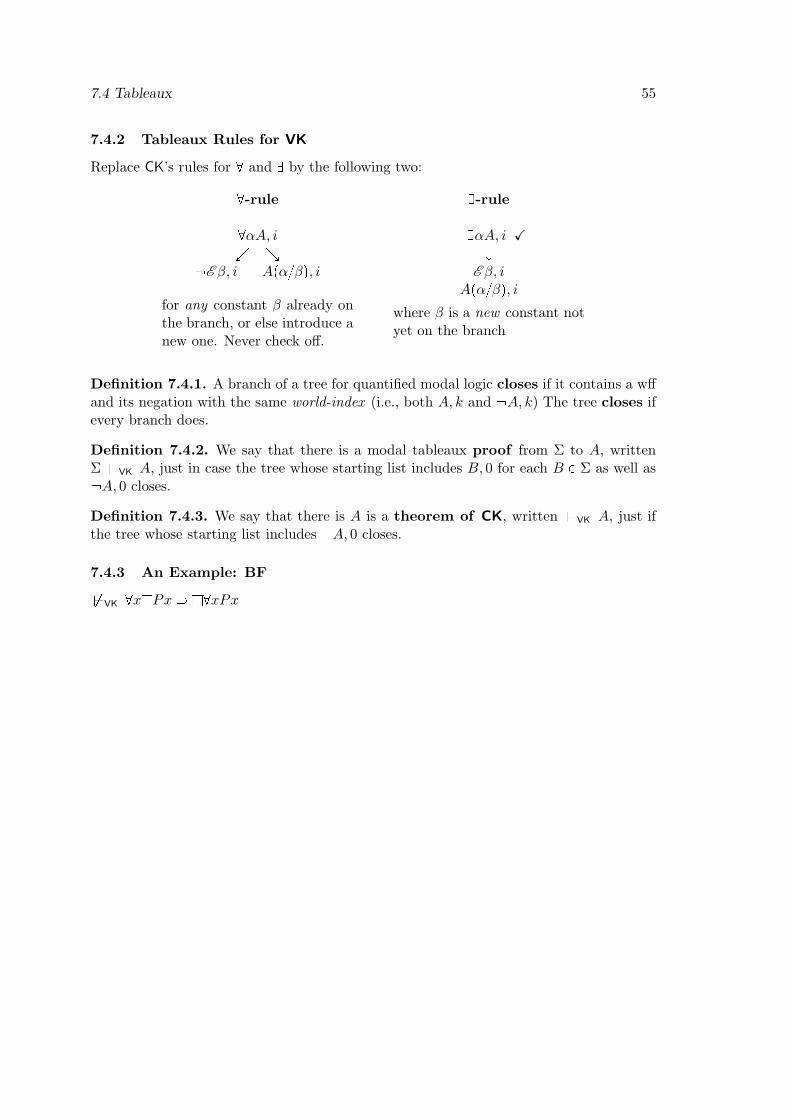
7.4.2 Tableaux Rules for VK
Replace CK’s rules for @ and D by the following two:
@-rule D-rule
@αA, i DαA, i XÖ × Ó
E β, i Apαβq, i E β, iApαβq, i
for any constant β already onthe branch, or else introduce anew one. Never check off.
where β is a new constant notyet on the branch
Definition 7.4.1. A branch of a tree for quantified modal logic closes if it contains a wffand its negation with the same world-index (i.e., both A, k and A, k) The tree closes ifevery branch does.
Definition 7.4.2. We say that there is a modal tableaux proof from Σ to A, writtenΣ $VK A, just in case the tree whose starting list includes B, 0 for each B P Σ as well as A, 0 closes.
Definition 7.4.3. We say that there is A is a theorem of CK, written $VK A, just ifthe tree whose starting list includes A, 0 closes.
7.4.3 An Example: BF
&VK @xlPx l@xPx
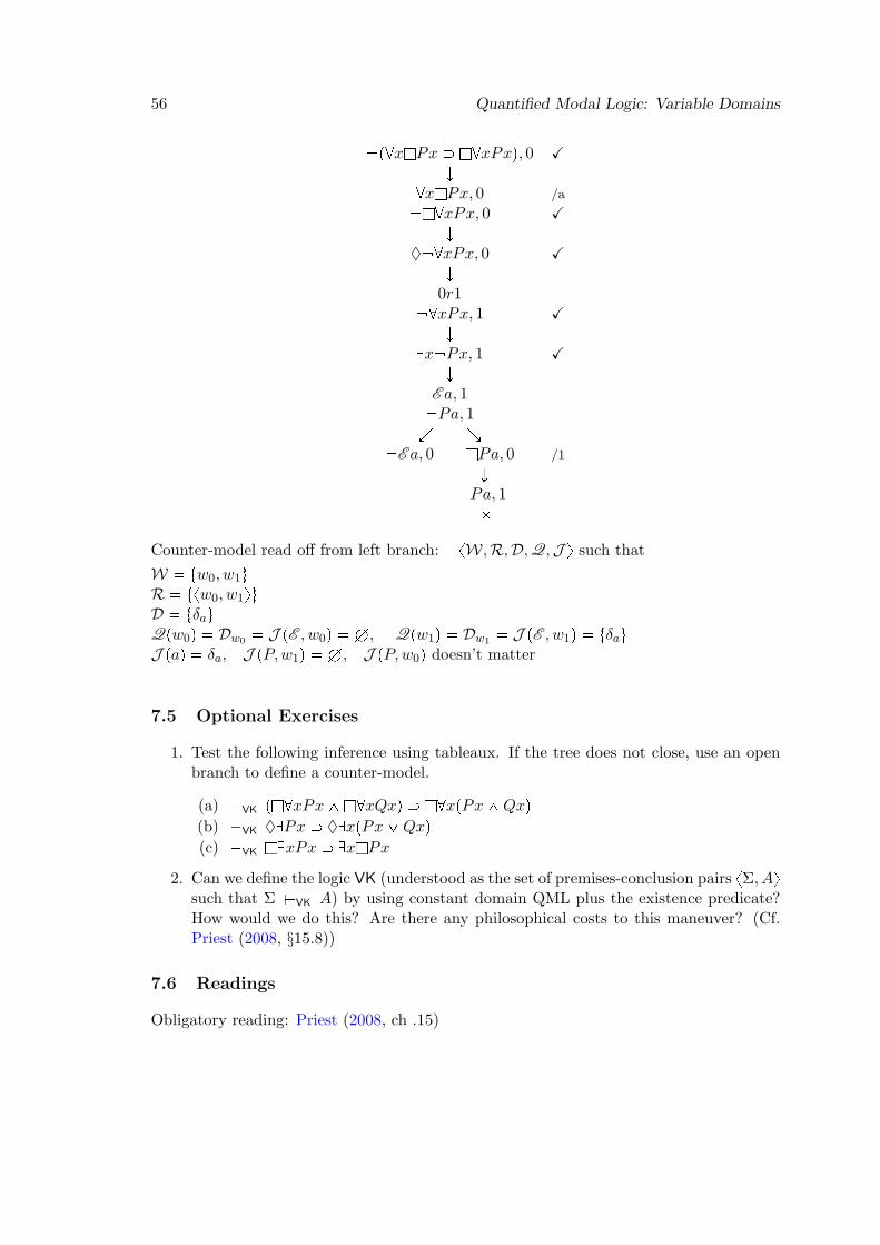
56 Quantified Modal Logic: Variable Domains
p@xlPx l@xPxq, 0 XÓ
@xlPx, 0 /a
l@xPx, 0 XÓ
@xPx, 0 XÓ
0r1 @xPx, 1 X
ÓDx Px, 1 X
ÓE a, 1 Pa, 1Ö ×
E a, 0 lPa, 0 /1
ÓPa, 1
Counter-model read off from left branch: xW,R,D,Q,J y such that
W tw0, w1uR txw0, w1yuD tδauQpw0q Dw0 J pE , w0q H, Qpw1q Dw1 J pE , w1q tδauJ paq δa, J pP,w1q H, J pP,w0q doesn’t matter
7.5 Optional Exercises
1. Test the following inference using tableaux. If the tree does not close, use an openbranch to define a counter-model.
(a) $VK pl@xPx^l@xQxq l@xpPx^Qxq
(b) $VK DPx DxpPx_Qxq(c) $VK lDxPx DxlPx
2. Can we define the logic VK (understood as the set of premises-conclusion pairs xΣ, Aysuch that Σ $VK A) by using constant domain QML plus the existence predicate?How would we do this? Are there any philosophical costs to this maneuver? (Cf.Priest (2008, §15.8))
7.6 Readings
Obligatory reading: Priest (2008, ch .15)

7.6 Readings 57
Optional readings:
• Priest (2008, §§13.1-13.6)
• Sider (2010, §9.6)
• Garson, James (2013.‘Modal Logic’. The Stanford Encyclopedia of Philosophy (Spring2013 Edition), Edward N. Zalta (ed.), URL = ¡http://plato.stanford.edu/archives/spr2013/entries/logic-modal/¿

Part III
Conditionals
59

8 Material and Strict Implication
8.1 What Are Conditionals?
Priest (2008, 11) — a characterization from philosophical logic:
‘Conditionals relate some proposition (the consequent) to some other proposi-tion (the antecedent) on which, in some sense, it depends.’
von Fintel (2011, 2) — a characterization from linguistic semantics:
‘Conditionals are sentences that talk about a possible scenario that may or maynot be actual and describe what (else) is the case in that scenario; or, con-sidered from “the other end”, conditionals state in what kind of possible scen-arios a given proposition is true. The canonical form of a conditional is a two-part sentence consisting of an “antecedent” (also: “premise”, “protasis”) [inEnglish] marked with if and a “consequent” (“apodosis”) sometimes markedwith then. . . ’
8.1.1 Conditionals in Natural Language (English)
Conditionals can be expressed in different ways in English. The ‘canonical’ form of aconditional is the one in (8.1), but see also (8.2)-(8.7)
(8.1) If Grijpstra played his drum, de Gier played his flute.
(8.2) Had he admitted his guilt, he would have gotten off easier.
(8.3) Take another step and I’ll knock you down.
(8.4) You won’t eat those and live.
(8.5) He was pushed or he wouldn’t have fallen down the cliff.
(8.6) Without you, I would be lost.
61
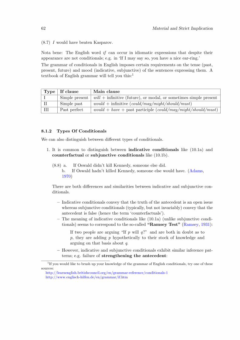
62 Material and Strict Implication
(8.7) I would have beaten Kasparov.
Nota bene: The English word if can occur in idiomatic expressions that despite theirappearance are not conditionals; e.g. in ‘If I may say so, you have a nice ear-ring.’
The grammar of conditionals in English imposes certain requirements on the tense (past,present, future) and mood (indicative, subjunctive) of the sentences expressing them. Atextbook of English grammar will tell you this:1
Type If clause Main clause
I Simple present will + infinitive (future), or modal, or sometimes simple present
II Simple past would + infinitive (could/may/might/should/must)
III Past perfect would + have + past participle (could/may/might/should/must)
8.1.2 Types Of Conditionals
We can also distinguish between different types of conditionals.
1. It is common to distinguish between indicative conditionals like (10.1a) andcounterfactual or subjunctive conditionals like (10.1b).
(8.8) a. If Oswald didn’t kill Kennedy, someone else did.b. If Oswald hadn’t killed Kennedy, someone else would have. (Adams,1970)
There are both differences and similarities between indicative and subjunctive con-ditionals.
– Indicative conditionals convey that the truth of the antecedent is an open issuewhereas subjunctive conditionals (typically, but not invariably) convey that theantecedent is false (hence the term ‘counterfactuals’).
– The meaning of indicative conditionals like (10.1a) (unlike subjunctive condi-tionals) seems to correspond to the so-called “Ramsey Test” (Ramsey, 1931):
If two people are arguing “If p will q?” and are both in doubt as top, they are adding p hypothetically to their stock of knowledge andarguing on that basis about q.
– However, indicative and subjunctive conditionals exhibit similar inference pat-terns; e.g. failure of strengthening the antecedent:
1If you would like to brush up your knowledge of the grammar of English conditionals, try one of thesesources:
http://learnenglish.britishcouncil.org/en/grammar-reference/conditionals-1http://www.englisch-hilfen.de/en/grammar/if.htm
8.1 What Are Conditionals? 63
AÑ B ÷ pA^ Cq Ñ B)
(Let’s agree on a useful notational convention and say that ‘Ñ’ stands forthe conditional, independently (i) of the natural language expressions used toexpress it (e.g. if ) and/or (ii) of the logical connective used to express theconditional.)
– Here are examples of the failure of antecedent strengthening:
(8.9) a. If I light this match, it will burn.b. ÷ If I light this match and it is wet, it will burn.
(8.10) a. If Piedro had come to the parade, he would have seen the dancers.b. ÷ If Piedro had come to the parade and got stuck behind a tallperson, he would have seen the dancers.
2. There are more types of conditionals than indicative/subjunctive conditionals. Forinstance, there are biscuit conditionals (or ‘speech act conditionals’) like (8.11)and (8.12.
(8.11) There are biscuits on the sideboard if you want them. (Austin)
(8.12) I paid you back yesterday, if you remember. (P.T. Geach p.c. to Austin)
Biscuit conditionals do not state conditions under which the consequent is true.Instead, they seem to operate on a speech act level.
3. There are also premise conditionals like (8.13) that often echo someone else’sintroduction of the antecedent.
(8.13) If you’re so clever, why don’t you do this problem on your own.
• Furthermore, besides conditional statements, there are conditional commands, prom-ises, offers, questions, etc.:
(8.14) If it gets cold, close the window and turn on the heating.
(8.15) I promise to buy you a car if you pass the driving test this time.
(8.16) What should I do if she doesn’t say ‘Yes’?
• Finally, note that there is still controversy over how to best classify conditionals. Forinstance, some theorists doubt that the indicative/subjunctive distinction is trackinga real semantic distinction (see e.g. Gibbard (1981, 222-6)).
8.1.3 Contrapositive, Converse, Inverse
• The contrapositive of AÑ B is B Ñ A
• N.B.: (C A B B A.
• The converse of AÑ B is B Ñ A.
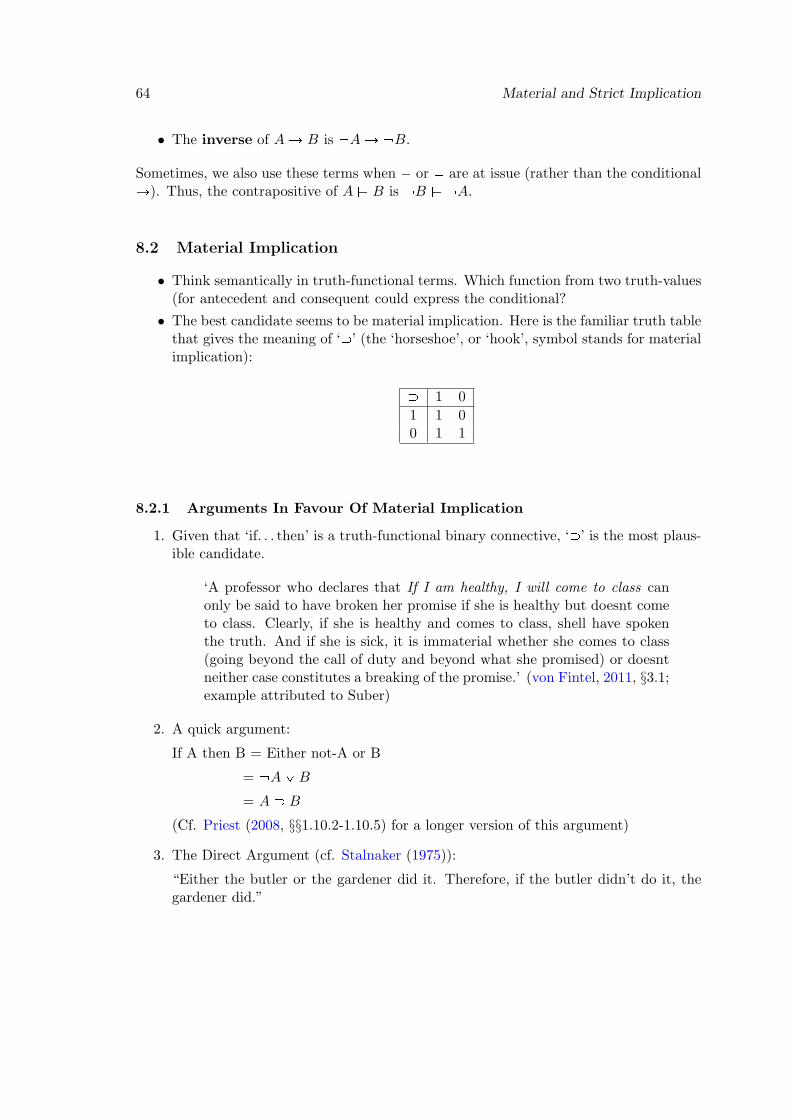
64 Material and Strict Implication
• The inverse of AÑ B is AÑ B.
Sometimes, we also use these terms when $ or ( are at issue (rather than the conditionalÑ). Thus, the contrapositive of A $ B is B $ A.
8.2 Material Implication
• Think semantically in truth-functional terms. Which function from two truth-values(for antecedent and consequent could express the conditional?
• The best candidate seems to be material implication. Here is the familiar truth tablethat gives the meaning of ‘’ (the ‘horseshoe’, or ‘hook’, symbol stands for materialimplication):
1 0
1 1 00 1 1
8.2.1 Arguments In Favour Of Material Implication
1. Given that ‘if. . . then’ is a truth-functional binary connective, ‘’ is the most plaus-ible candidate.
‘A professor who declares that If I am healthy, I will come to class canonly be said to have broken her promise if she is healthy but doesnt cometo class. Clearly, if she is healthy and comes to class, shell have spokenthe truth. And if she is sick, it is immaterial whether she comes to class(going beyond the call of duty and beyond what she promised) or doesntneither case constitutes a breaking of the promise.’ (von Fintel, 2011, §3.1;example attributed to Suber)
2. A quick argument:
If A then B = Either not-A or B
= A_B
= A B
(Cf. Priest (2008, §§1.10.2-1.10.5) for a longer version of this argument)
3. The Direct Argument (cf. Stalnaker (1975)):
“Either the butler or the gardener did it. Therefore, if the butler didn’t do it, thegardener did.”
8.2 Material Implication 65
(i) ‘A _ B’ entails ‘If A, then B’. Substitute ‘ A’ for ‘A’. ‘ A _ B’ entails ‘if Athen B’; i.e. ‘A B’ entails ‘if A then B’.
(ii) It is widely accepted that the indicative conditional entails the material condi-tional; that is, ‘If A then B’ entails ‘A B.So we get the equivalence of ‘If A then B’ and ‘A B’.
8.2.2 Arguments Against Material Implication
1. The analysis of conditionals as expressing material implication gives rise to the so-called “paradoxes of material implication”.2 Take another look at the truthtable: the falsity of the antecedent is sufficient for the truth of the conditional, andso is the truth of the consequent.
Positive Paradox of MI: B (C A B
Negative Paradox of MI: A (C A B
Ad 1: Suppose (correctly) that the SPO is in the Austrian government. Does itfollow from this that if people go to the elections, then the SPO is in the Austriangovernment?
Ad 2: Suppose (correctly) that there aren’t 25 people in the room. Does it followfrom this that if there are 25 people in the room, then there are 50 people in theroom?
2. The analysis also has problems with embedded conditionals. For instance, con-sider cases where indicative conditionals are embedded under nominal quantifiers:
(8.17) a. Every student will succeed if he works hard.b. No student will succeed if he goofs off.
The material implication analysis may make the correct predictions for (9.6a), butit predicts that (9.6b) means that every students goofs off and does not succeed(Higginbotham, 1986): The analysis of (9.6b) is DxpSx^Gx Uxq— equivalently,@x pSx^Gx Uxq and @xpSx^Gx^ Uxq.
3. There are indicative/subjunctive pairs such as (10.1a) and (10.1b), which havethe same antecedent and consequent, yet one may be true and the other false. Sothey cannot both be expressed by material implication.
2In logic, a proposition or statement counts as paradoxical if it is self-contradictory and its obviousalternatives are either self-contradictory or very costly (e.g. the Liar paradox). A thumbnail definition of‘paradox’ in philosophy: a paradox is a set of propositions, or sentences, all of which seem true/acceptablebut which are mutually inconsistent. The ‘paradoxes of material implications’ are not strictly paradoxes ineither of these senses, but rather shortcomings in the match between the formal analysis and our intuitivejudgments regarding (instances of) conditionals (in natural language).
66 Material and Strict Implication
4. Material implication validates a number of inference patterns that intuitively aren’tvalid for conditionals.
(8.18) A B (C pA^ Cq B (strengthening of the antecedent)
(8.19) pA^Bq C (C pA Cq _ pB Cq
(8.20) pA Bq ^ pC Dq (C pA Dq _ pC Bq
(8.21) pA Bq (C A
(8.22) pA Bq (C B
5. Hunter’s counterexample is an instance of (9.4):
Tax man: If you filled in your tax form incorrectly and owe the Governmentmoney, you intended to cheat the Government.
Tax payer: Thats not true!Tax man: So you admit you filled in your tax form incorrectly and owe the
Government money!
8.2.3 A Sophisticated Defence of Material Implication
Next time well will look at a famous attempt at defending the claim that if. . . (then) means. It draws a principled distinction between semantics and pragmatics and argues thatif. . . (then) semantically means (even if pragmatically, it conveys more). This attemptis due to Grice (1975) and Jackson (1979).
8.3 Strict Implication
• Material implication makes implication a contingent affair: If A and B happen tobe true, then both A B and B A are also true.
• Lewis (1917, 355): “‘Proof’ requires that a connection of content or meaning or lo-gical connection be established. And this is not done for the postulates and theoremsin material implication . . . For a relation which does not indicate relevance of contentis merely a connection of ‘truth-values’, not what we mean by a ‘logical’ relation or‘inference’.”
• According to C. I. Lewis, material implication does not capture any ‘logical’ connec-tion between antecedent and consequent. But it seems that a conditional says thatthe consequent must follow from the premises – there is a connection of necessity.What captures the idea that A implies B is A B’s being necessarily true. Strictimplication, p J q means: A B is necessarily true.
A J B df. lpA Bq
8.3 Strict Implication 67
• Strict implication is immune to a number of the objections raised against the materialconditional above. For example:
(8.23) B *K A J B (cf. paradox of MI)
(8.24) A *K A J B (cf. paradox of MI)
(8.25) pA^Bq J C *K pA J Cq _ pB J Cq(8.26) pA J Bq ^ pC J Dq *K pA J Dq _ pC J Bq(8.27) pA J Bq *K A
(8.28) pA J Bq *K B
These are all valid with in place of J. However, there is an analogous set ofconcerns that can be raised about the strict conditional.
8.3.1 The Paradoxes of Strict Implication and Other Problems
1. The Paradoxes of Strict Implication:
Positive Strict Paradox: lB (K pA J Bq
Negative Strict Paradox: A (K pA J Bq
Counter-examples: If April is rainy, then 2 is the only even prime number.If there are no even prime numbers, the Greens will win the next elections.
2. Reasoning with necessities and impossibilities.
By the Positive Strict Paradox, as soon as we reason with consequents that arenecessary, we get true conditionals – no matter the antecedent. And by the NegativeStrict Paradox, as soon as we reason with antecedents that are impossible, we gettrue conditionals – no matter the consequent. But reasoning with necessary and/orimpossible propositions is essential to many areas of inquiry: mathematics, logic,(parts of) philosophy, etc.
3. Explosion:
A ^ A is a contradiction; it isn’t true at any world. So it is impossible. Hence(K pA ^ Aq J B. By modus ponens, we have A ^ A (KJ B. This meansthat contradictions entail everything. But sometimes, we may need to reason withcontradictions. A logic in which anything follows from contradictions is of no use inthis case (cf. Priest (2008, §4.8) for examples of reasoning with contradictions).
68 Material and Strict Implication
8.3.2 In Defense of Strict Implication
C.I. Lewis accepted the Positive and Negative Strict Paradoxes as “sound logical prin-ciples”, even though they at first appear “not in accord with the ‘proper’ sense of implies”(C.I. Lewis, A Survey of Symbolic Logic, 1918, p. 339). His argument for Negative StrictParadox runs (Lewis and Langford, Symbolic Logic pp. 250-1):
Suppose A^ Athen A by conjunction elimination
so A_B by disjunction introductionBut A by conjunction elimination again
So B by disjunctive syllogism (A, A_B $ B)
which assumes that any impossible proposition can be put in the form of an explicitcontradiction, A^ A. He also produced a proof for Positive Strict Paradox:
Suppose Athen pA^Bq _ pA^ Bq
so A^ pB _ Bq by distributionSo B _ B by conjunction elimination
this time assuming that any necessary proposition can be put in the form B _ B.
8.4 Optional Exercises
1. (a) Show that the inference patterns in §2.2, (9.1) – (9.5), are valid in classicalpropositional logic.
(b) Find English (or German) natural language instances of the inference patternsin §2.2, (9.1) – (9.5), which show that the patterns are intuitively invalid.
(c) Consider the inference patterns in §2.2, (9.1) – (9.5): Are the premises alsosemantic consequences of the conclusions? (That is, e.g., does the followinghold: pA^Cq B (C A B?) In each case, is this result in accordance withyour judgments about conditionality?
2. Check, by using tableaux, whether the inference patterns in (8.23) – (8.28) are invalidin normal modal logics stronger than K.(Hint: (i) Replace any formula ‘A J B’ with ‘lpA Bq’ on the tree. (ii) Try S5first and go from stronger to weaker logics: If an inference pattern is invalid in astronger system, it is invalid in a weaker system.)
3. Which of the objections against material implication are also strong objectionsagainst strict implication?
4. Can you think of further inference patterns that are valid with (a) material implic-ation or (b) strict implication and which are intuitively invalid? Give examples toillustrate their intuitive invalidity.

8.5 Readings 69
8.5 Readings
Sources of this handout:
• von Fintel (2011) — optional reading
• Priest (2008, §§1.6–1.10, 4.5–4.9) — obligatory reading
• Edgington, Dorothy: Conditionals. The Stanford Encyclopedia of Philosophy (May2014), Edward Zalta (ed.), URL = http://plato.stanford.edu/entries/conditionals/,sections 1-2

9 Grice’s Defense of Material Implication
9.1 Material Implication
• Material implication: ‘A B’ is true if either A is false or B is true; it is false if Ais true and B is false.
• Among the truth-functional, two-place connectives, material implication is the mostplausible candidate for the conditional.
‘A professor who declares that If I am healthy, I will come to class canonly be said to have broken her promise if she is healthy but doesnt cometo class. Clearly, if she is healthy and comes to class, shell have spokenthe truth. And if she is sick, it is immaterial whether she comes to class(going beyond the call of duty and beyond what she promised) or doesntneither case constitutes a breaking of the promise.’ (von Fintel, 2011, §3.1;example attributed to Suber)
• For arguments in favour of the material implication account of conditionals, seeHandout V-1, §2.1.
9.2 The Equivalence Thesis
9.2.1 The Unsupplemented Equivalence Thesis and its Problems (Review)
Unsupplemented Equivalence Thesis: The meaning of natural-language indicativeconditionals is material implication.
Some of the main problems with the Unsupplemented Equivalence Thesis (see HandoutV-1 for details):
1. Paradoxes of material implication.
71
72 Grice’s Defense of Material Implication
Positive Paradox: B (C A B
Negative Paradox: A (C A B
2. Material implication validates a number of intuitively invalid inference pat-terns.
(9.1) A B (C pA^ Cq B (strengthening of the antecedent)
(9.2) pA^Bq C (C pA Cq _ pB Cq
(9.3) pA Bq ^ pC Dq (C pA Dq _ pC Bq
(9.4) pA Bq (C A
(9.5) pA Bq (C B
3. Embedded conditionals. E.g., indicative conditionals embedded under nominalquantifiers:
(9.6) a. Every student will succeed if he works hard.b. No student will succeed if he goofs off.
9.2.2 The Supplemented Equivalence Thesis
Grice (1975) and Jackson (1979) defend the following thesis:
The Supplemented Equivalence Thesis: The semantic, conventional meaning ofnatural-language indicative conditionals is material implication.
The basic idea: ‘If A then B’ literally (semantically, conventionally) means A B.However, it pragmatically implicates that there is a connection between A and B. So aliterally true indicative conditional may still fail to be assertable because it implicates afalse proposition.
9.3 Grice on Communication
• What is said: The notion of what someone has said is closely related to the con-ventional (=semantic) meaning of the words (the sentence) she has uttered.
What the speaker said involves some pragmatic mechanisms: For a full identific-ation of what the speaker of “He is in the grip of a vice” has said, one needs to knowwhat ‘he’ refers to, the time of utterance, the meaning, on the particular occasionof utterance, of the phrase in the grip of a vice (resolution of ambiguity).
• Implicature: The implicatures generated by an utterance of a sentence are thepropositions that are intentionally communicated by the speaker with her utterance,but are not part of what is said by the sentence in the context of use.
• Conversational implicature:
9.3 Grice on Communication 73
– Conversational implicatures are propositions communicated by an utterance invirtue of what is said together with general facts about the context and conver-sational norms. Conversational implicatures are cancelable and non-detachable.
– Grice (1975, 31):
A man who, by (in, when) saying (or making as if to say) that p hasimplicated that q, may be said to have conversationally implicatedthat q, provided that (1) he is to be presumed to be observing theconversational maxims, or at least the Cooperative Principle; (2) thesupposition that he is aware that, or thinks that, q is required in orderto make his saying or making as if to say that p (or doing so in thoseterms) consistent with this presumption; and (3) the speaker thinks(and would expect the hearer to think that the speaker thinks) that itis within the competence of the hearer to work out, or grasp intuitively,that the supposition mentioned in (2) is required.
– Examples:
(9.7) In a letter of reference for a philosophy PhD student, “Smith hasbeautiful handwriting and was never late for class.”ñ Implicature: Smith is not a good philosopher.
(9.8) A: I am out of petrol.B: There is a garage around the corner.ñ Implicature: The garage is open and selling petrol.
• The general principle: The Cooperative Principle
Make your conversational contribution such as is required, at the stage atwhich it occurs, by the accepted purpose or direction of the talk exchangein which you are engaged.
• 4 Categories of Maxims
1. Maxim of Quantity:
a) Make your contribution as informative as is required (for the current pur-poses of the exchange).
b) Do not make your contribution more informative than is required.
2. Maxim of Quality:
Supermaxim: “Try to make your contribution one that is true”
a) Do not say what you believe to be false.
b) Do not say that for which you lack adequate evidence.
3. Maxim of Relation:
Be relevant.
4. Maxim of Manner:
Supermaxim: “Be perspicuous”
74 Grice’s Defense of Material Implication
a) Avoid obscurity of expression.
b) Avoid ambiguity.
c) Be brief (avoid unnecessary prolixity).
d) Be orderly.
• Four ways in which one can fail to fulfill a maxim:
1. Violate a maxim: quietly and unostentatiously, in some cases liable to mislead
2. Opt out from the operation of the maxim and of the Cooperative Principleby saying/indicating that one is unwilling to cooperate in the way the maximrequires.
3. Be faced with a clash: be unable to fulfill one maxim without violating another.
4. Flout a maxim: blatantly fail to fulfill the maxim.“On the assumption that the speaker is able to fulfill the maxim and to do sowithout violating another maxim (because of a clash), is not opting out, and isnot, in view of the blatancy of his performance, trying to mislead, the heareris faced with a minor problem: How can the speaker’s saying what he did saybe reconciled with the supposition that he is observing the overall CooperativePrinciple? This situation is one that characteristically gives rise to a conversa-tional implicature; and when a conversational implicature is generated in thisway, I shall say that a maxim is being exploited.” (Grice, 1975, 30)
• Two primary features of conversational implicatures:
1. Cancelability
A conversational implicature can be canceled, explicitly or ‘contextually’ (Grice,1975, 39): It can be (made) clear that the speaker is opting out.
(9.9) a. A: X is meeting a woman this evening.ñ Usual generalized conversational implicature: the person X is meetingis not X’s wife, mother, sister, or perhaps even close platonic friend.b. B: X is meeting a woman this evening, who is in fact his sister.
2. Non-detachability
“it will not be possible to find another way of saying the same thing, whichsimply lacks the implicature in question” (Grice, 1975, 39)
(9.10) a. A: X is meeting a woman this evening.b. B: X is meeting a member of the female gender this evening.ñ Generalized conversational implicature in both cases: the person X ismeeting is not X’s wife, mother, sister, or perhaps even close platonicfriend.
• Conventional implicature: the conventional meaning of the words used determine(besides helping to determine what the speaker says) what is implicated.
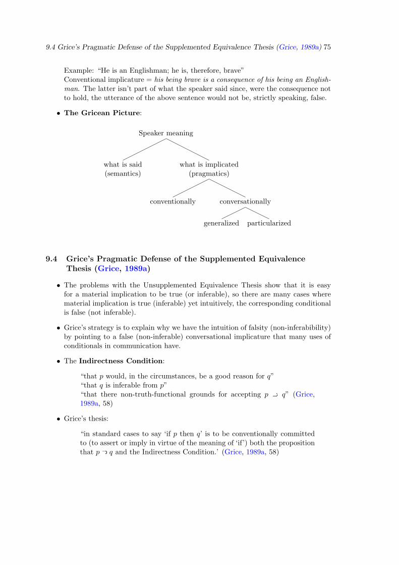
9.4 Grice’s Pragmatic Defense of the Supplemented Equivalence Thesis (Grice, 1989a) 75
Example: “He is an Englishman; he is, therefore, brave”Conventional implicature = his being brave is a consequence of his being an English-man. The latter isn’t part of what the speaker said since, were the consequence notto hold, the utterance of the above sentence would not be, strictly speaking, false.
• The Gricean Picture:
Speaker meaning
what is said(semantics)
what is implicated(pragmatics)
conventionally conversationally
generalized particularized
9.4 Grice’s Pragmatic Defense of the Supplemented EquivalenceThesis (Grice, 1989a)
• The problems with the Unsupplemented Equivalence Thesis show that it is easyfor a material implication to be true (or inferable), so there are many cases wherematerial implication is true (inferable) yet intuitively, the corresponding conditionalis false (not inferable).
• Grice’s strategy is to explain why we have the intuition of falsity (non-inferabibility)by pointing to a false (non-inferable) conversational implicature that many uses ofconditionals in communication have.
• The Indirectness Condition:
“that p would, in the circumstances, be a good reason for q”“that q is inferable from p”“that there non-truth-functional grounds for accepting p q” (Grice,1989a, 58)
• Grice’s thesis:
“in standard cases to say ‘if p then q’ is to be conventionally committedto (to assert or imply in virtue of the meaning of ‘if’) both the propositionthat p q and the Indirectness Condition.’ (Grice, 1989a, 58)
76 Grice’s Defense of Material Implication
ñ Grice ultimately argues that in ‘standard’ uses of ‘if p then q’ a speaker literallysays that p q and conversationally implicates the Indirectness Condition.
• Grice (1989a, 61-2):
To say that p q is to say something logically weaker than to deny thatp or to assert that q, and is thus less informative; to make a less inform-ative rather than a more informative statement is to offend against thefirst maxim of Quantity, provided that the more informative statement,if made, would be of interest. There is a general presumption that inthe case of “p q”, a more informative statement would be of interest.No one would be interested in knowing that a particular relation (truth-functional or otherwise) holds between two propositions concerned, unlesshis interest were of an academic or theoretical kind [. . . ] An infringementof the first maxim of Quantity, given the assumption that the principle ofconversational helpfulness is being observed, is most naturally explainedby the supposition of a clash with the second maxim of Quality (“Haveadequate evidence for what you say”), so it is natural to assume that thespeaker regards himself as having evidence for the less informative state-ment (that p q)—that is, non-truth-functional evidence. So standardlyhe implicates that there is non-truth-functional evidence when he says thatp q;
• Let’s spell this out:
1. ‘ p’ and ‘q’ are more informative than ‘p q.’
2. In general, we are not interested in the connection between the propositionsthat p and that q without being interested in their truth values.
3. So in asserting ‘p q’, a speaker standardly fails to observe the maxim ofQuantity (“make your contribution as informative as is required. . . ”): it willstandardly give the hearer less information than she would like.
4. If it can be supposed that the speaker is trying to observe the CooperativePrinciple, the failure to comply with Quantity is best explained by the factthat she would infringe on the maxim of Quality (“do not say that for whichyou lack adequate evidence”), were she to make a stronger claim than ‘p q.’
5. So the speaker must (take herself to) have only non-truth-functional evidencefor a connection between the propositions that p and that q.
6. So the speaker is conversationally implicating that there is non-truth-functionalevidence for a connection between the propositions that p and that q (Indirect-ness Condition).
Note the similarities with what Grice (1975, 32-3, example 3) labels ‘Group B’examples of conversational implicatures, in which the maxim of Quantity is infringedupon and where this infringement is to be explained by the supposition of a clashwith the maxim of Quality.
9.4 Grice’s Pragmatic Defense of the Supplemented Equivalence Thesis (Grice, 1989a) 77
• Grice contends that the Indirectness Condition fulfills the two primary features ofconversational implicatures:
1. Cancelability:
a) Explicit cancelation: “To say ‘If Smith is in the library, he is working’would normally carry the implication of the Indirectness Condition; but Imight say (opting out) ‘I know just where Smith is and what he is doing,but all I will tell you is that if he is in the library he is working.”’ (Grice,1989a, 59)
b) Contextual cancelation: there are cases in which the Indirectness Conditionis simply absent:
(9.11) Perhaps if he comes, he will be in a good mood.(9.12) See that, if he comes, he gets his money. (Grice, 1989a, 60)
Note: Biscuit conditionals are also uses of conditionals that do not conveythe Indirectness Condition.
2. Non-detachability:
(9.13) Either Smith is not in London, or he is attending the meeting.
(9.14) It is not the case that Smith is both in London and not attending themeeting.
According to Grice, (9.13) and (9.14) – both of which say the same as ‘If Smithis in London, he’s attending the meeting’ (they’re truth-functionally equivalentwith ‘Smith is in London Smith is attending the meeting’) – also implicatethe Indirectness Condition.
Grice’s Defense and the Problems of the Unsupplemented Equivalence Thesis
1. Paradoxes of material implication
Explanandum for Grice: why instances of the paradoxes strike us as unassert-able/false despite their literal truth.
(9.15) If there are 25 people in the room, then there are 50 people in the room.
If the speaker has the information that there aren’t 25 people in the room (negativeparadox), an assertion of (9.15) infringes on the maxim of Quantity. Similarly, ifshe has the information that there are 50 people in the room (positive paradox). Ineither case, a false conversational implicature is generated: that there is evidence fora non-truth-functional connection between there being 25 people in the room andthere being 50 people in the room (Indirectness Condition). It is this implicaturethat explains our intuitive judgment that (9.15) is false/unassertible.
78 Grice’s Defense of Material Implication
9.5 Problems with Grice’s Defense
1. Conditionals in thought (Edgington, 1995, 245):
But the difficulties with the truth-functional conditional cannot be ex-plained away in terms of what is an inappropriate conversational remark.They arise at the level of belief. Believing that John is in the bar does notmake it logically impermissible to disbelieve “if he’s not in the bar he’s inthe library”. Believing you won’t eat them, I may without irrationalitydisbelieve “if you eat them you will die”. Believing that the Queen is notat home, I may without irrationality reject the claim that if she’s home,she will be worried about my whereabouts. As facts about the norms towhich people defer, these claims can be tested. But, to reiterate, the mainpoint is not the empirical one. We need to be able to discriminate believ-able from unbelievable conditionals whose antecedent we think false. Thetruth-functional account does not allow us to do this.
Note that Edgington’s criticism applies generally to pragmatic explanations of ourjudgments of truth (falsity) in terms of judgements about (un)assertability that tar-get conversational implicatures. The point seems to be independent of a pragmaticdefense of conditionals.
2. Contraposition
(9.16) a. Even if the Bible was divinely inspired, it is still not literally true.b. If the Bible is literally true, then it is not divinely inspired. (Bennett)
(9.17) a. If it rains, it will not rain heavily.b. If it rains heavily, it will not rain. (Jackson)
Material implication validates contraposition: A B (C B A.
(9.16a) and (9.16b) make it intuitively plausible that ‘If A then B’ and ‘If not-Bthen not-A’ do not have the same truth conditions: (9.16a) can be true and (9.16b)false (the same holds of (9.17a/b)). However, Grice’s strategy cannot explain thisdifference in truth/assertability judgments (‘If A then B’ and ‘If not-B then not-A’are equally ‘logically strong’ and so equally informative).
3. Disanalogies in assertibility between if. . . then and or (Grice, 1975, 63)
‘A B’ is logically equivalent with ‘ A_B’ and according to Grice, the literal mean-ing of ‘or’ is truth-functional disjunction (‘_’). Thus, a speaker should standardlyimplicate the Indirectness Condition with uses of ‘or’ just as much as she implicatesit with standard uses of ‘if. . . (then)’. But there are important differences, as Grice(1989a, 63) himself remarks: “whereas . . . a disjunctive statement which has beenadvanced on non-truth-functional grounds can be confirmed truth-functionally, byestablishing one of its disjuncts, the parallel idea with regard to conditionals is notacceptable.” For illustration:
9.6 Readings 79
(9.18) a. Either Wilson won the elections or Thorpe did.b. That’s right. In fact, Wilson won.
(9.19) a. If Wilson didn’t win, then Thorpe did.b. ? That’s right. In fact, Wilson won.
4. Negations of indicative conditionals
The literal meaning of a negated conditional ‘It is not the case that if A, then B’ is pA Bq. The latter is logically equivalent to A^ B. However, it seems that weoften assert the negation of a conditional and say, or implicate, neither A nor not-B.
(9.20) Speaker A: If God exists, we are free to do whatever we like.Speaker B: That’s not the case.
We can take speaker B’s assertion to be short for ‘It is not the case that if Godexists, we are free to do whatever we like.’ But it seems unreasonable to understandB as saying (implicating) that God exists and we are not free to do whatever welike. (Grice (1989a, 80-1) noticed this problem and attempted to solve it by arguingthat with negations of conditionals, we either in fact assert ‘A B’ (the negationtakes narrow scope) or deny the conversational implicature that there is non-truth-functional evidence for the material implication.)
9.6 Readings
• Grice (1975)
• Optional: Bennett (2003, pp. 20–27) [N.B.: In his exposition of Grice on indicativeconditionals on pp. 24-5, Bennett is mistakenly appealing to the maxims of quantity(1a) and manner (4c) instead of quantity (1a) and quality (2b). See Grice (1989a,61-2) for this point.]
• More on Grice’s defense of the Supplemented Equivalence Thesis: Grice (1989a)
• Jackson’s pragmatic defense of the equivalence thesis: Jackson (1979)

10 Stalnaker’s Theory of Conditionals
10.1 The Direct Argument
• Stalnaker’s example: ‘Either the butler or the gardener did it. Therefore, if thebutler didn’t do it, the gardener did.’ (Stalnaker, 1975, 63)
• (i) or-to-if: ‘A_B’ entails ‘If A, then B’. Substitute ‘ A’ for ‘A’. ‘ A_B’ entails‘if A then B’; i.e. ‘A B’ entails ‘if A then B’.
(ii) It is widely accepted that the indicative conditional entails the material condi-tional; that is, ‘If A then B’ entails ‘A B.So we get the equivalence of ‘If A then B’ and ‘A B’ (cf. Handout V-1, §2.1).
• But there are well-known problems with the claim that ‘If A then B’ and ‘A B’are equivalent – for example, the paradoxes of material implication are valid.
• Stalnaker: there are two options that make use of the distinction between semanticsand pragmatics.
1. Grice’s strategy: Defend the semantic equivalence of ‘If A then B’ and ‘A B’,and explain pragmatically why those inferences (e.g. the paradoxes of MI) seeminvalid (see Handout V-2 ).
2. Stalnaker’s strategy: Reject the material conditional analysis in favour of astronger semantic account of If. . . (then), and explain pragmatically why thedirect argument seems valid.
Stalnaker defines a semantic notion of entailment and a pragmatic notion ofreasonable inference and shows that, while the premise of the direct argument(‘A or B’) doesn’t entail the conclusion (‘If not-A, B’), the conclusion canreasonably be inferred from the premise.
81
82 Stalnaker’s Theory of Conditionals
10.2 Pragmatics
• Inquiring, deliberating, . . . , exchanging information (communication): one is essen-tially distinguishing between alternative ways the world could be – between differentpossible worlds.
• Propositions =df. functions from possible worlds into truth values (true and false),or equivalently sets of possible worlds (those at which the proposition is true)
Example: The proposition that snow is white is a function that takes every world atwhich snow is white into true, and every other world into false. Equivalently: tw:snow is white at wu
• Context set =df. the set of possible worlds not ruled out by the presupposed back-ground information
In conversation, participants make assumptions about what is common groundamong all the participants: they presuppose certain propositions. Suppose parti-cipants A and B both presuppose (in the above sense) propositions p and q. Thentheir context set is the intersection of p and q – it’s the set of possible worlds atwhich both p and q are true. If they haven’t established whether r, then their contextset contains some r-worlds and some not-r-worlds
• Assertion: It is an essential effect of assertion that they add the asserted propositionto the presupposed background information (if they’re accepted by all participants).That is, successful assertions of r have the effect of intersecting the context set withr. (To add r to the common ground p, q is to intersect the context set Cp,q with r:the context set after the successful assertion of r is Cp,q X r.)
• A proposition is compatible with a context iff it is true in some of the worlds inthe context set.Intuitively: the proposition is among the presuppositions corresponding to the con-text set (or is a consequence of those presuppositions).
• A proposition is entailed by a context iff it is true in all of the worlds in the contextset.Intuitively: the presuppositions corresponding to the context set determine that theproposition is true.
• In linguistic communication, speakers try to establish information by distinguishingbetween possible worlds in the context set. An increase in information correspondsto a reduction of possible worlds in the context set.
• Pragmatics has to do with assertability & acceptability of utterances. Semantics hasto do with truth and falsity of sentences (in context).
10.3 Semantics for Conditionals
• Stalnaker gives the same semantic analysis for indicative and subjunctive condition-als. Their difference is a pragmatic one.
10.3 Semantics for Conditionals 83
• Stalnaker’s basic idea:
‘The idea of the analysis is this: a conditional statement, if A, then B, isan assertion that the consequent is true, not necessarily in the world as itis but in the world as it would be if the antecedent were true.’
• Let’s make this formally more precise. We’re going to be a little more sloppy thanusual with the formal details (since we’ve got a lot to cover today). A rigorouspresentation of Stalnaker’s logic of conditionals, called C2, is given in his ‘A Theoryof Conditionals’ (1968), which we follow in this presentation. (See also Priest (2008,ch. 5) and Sider (2010, ch. 8).)
• C2 is a propositional modal logic (see Handout III-1 and III-2 ).
Definition 10.3.1. A model structure MS is a structure xW,R, λy, where
(i) W is a non-empty set of objects, intuitively understood as possible worlds
(ii) R is an accessibility relation between worlds
(iii) λ is the absurd world, at which contradictions and all their consequences are true.The following conditions apply: (a) λ PW. (b) It is not accessible from any worldsnor does it access any worlds: for any w, xλ,wy R R and xw, λy R R.(λ is needed for the interpretation of conditionals with impossible antecedents.)
• Selection function f : In addition to a model structure, the semantic apparatusincludes a selection function, f , which takes a proposition p and a world w as argu-ments and maps them to a unique world w1: fpp, wq w1.Intuitively, fpp, wq is the “closest”, or “most similar” world (to w) at which p is true.
• The semantic clause for the conditional, written ‘¡’, can be stated as follows:
A ¡ B is true at w if B is true at fpA,wq;A ¡ B is false at w if B is false at fpA,wq;
• The semantic clauses for the atomic case, for propositional connectives ( ,^,_,,) and modal operators (l,) are the standard ones (see Definition 3.3 on HandoutIII-1 ).
Definition 10.3.2. An inference is valid in system C2 iff every world of everymodel M of model structure MS at which the premises are true is one at which theconclusion is also true; i.e.
Σ (C2A iff for all worlds w PW of all models M of model structure MS :
if B is true at w in M for all the premises B P Σ, then A is true at w in M.
• Stalnaker lays down a number of conditions on the selection function f that aremeant to ensure that it yields the most similar world:
fpA,wq w1: call A the antecedent, w the base world, and w1 the selected world.
84 Stalnaker’s Theory of Conditionals
(1) For all antecedents A and base worlds w, A must be true at fpA,wq.
(2) For all antecedents A and base worlds w, fpA,wq λ only if there is no worldaccessible from w at which A is true.
N.B.: The absurd world is selected only when the antecedent is impossible.
(3) For all antecedents A and base worlds w, if A is true at w, then fpA,wq w.
N.B.: No world is more similar to w than w itself. So if A is true at w, w itselfis selected for the consideration of whether or not B is the case.
(4) For all antecedents B and B1 and base worlds w, if B is true at fpB1, wq andB1 is true at fpB,wq, then fpB,wq fpB1, wq.
N.B.: ‘The fourth condition ensures that the [similarity] ordering among pos-sible worlds is consistent in the following sense: if any selection established[world] β as prior to β1 in the ordering (with respect to a particular base worldα), then no other selection (relative to that α) may establish β1 as prior to β.’(Stalnaker, 1968, 105)
10.3.1 The Context-Dependence of Conditionals
• What does “closest”, or “most similar” mean? It will depend on the context: ‘Rel-evant respects of similarity are determined by the context.’ (Stalnaker, 1968, 69)
• Stalnaker (1975, 69) adds a fifth, contextual condition:
(5) If w is in the context set, then fpA,wq must, if possible, be within the contextset.
N.B.: ‘all worlds within the context set are closer to each other than any worldsoutside it.’ ‘The idea is that when a speaker says “If A,” then everything heis presupposing to hold in the actual situation is presupposed to hold in thehypothetical situation in which A is true.’
• Stalnaker (1975, 69):
‘The motivation for the principle is this: normally a speaker is concernedonly with possible worlds within the context set, since this set is defined asthe set of possible worlds among which the speaker wishes to distinguish.So it is at least a normal expectation that the selection function shouldturn first to these worlds before considering counterfactual worlds–thosepresupposed to be non-actual.’
• This makes the truth-conditions – here: the semantic content – of (indicative) con-ditionals context-dependent: they depend on the context in a way similar to howthe content, or reference, of a definite description or pronoun depends on the context(on who/what is being picked out by the expression in the context of utterance).1
1Note that Stalnaker uses the word ‘pragmatic’ in (Stalnaker, 1975, 69) in the sense introduced by R.Montague: pragmatics fills the gap between the context-invariant features of sentences and what a speaker
10.3 Semantics for Conditionals 85
10.3.2 Indicative vs Subjunctive Conditionals
• Stalnaker’ gives a single semantics for both indicative and subjunctive conditionals.But as we have seen (cf. example (8) on Handout V-1 ), two conditionals can differin truth value when they otherwise differ only in that one is in indicative mood, andthe other in subjunctive:
(10.1) a. If Oswald didn’t kill Kennedy, someone else did.b. If Oswald hadn’t killed Kennedy, someone else would have. (Adams,1970)
• So how does Stalnaker distinguish between indicative and subjunctive conditionals?
• The difference for Stalnaker is in their context-dependence. The subjunctive mood,he claims, suspends the pragmatic condition (5) on the selection function, which is‘only a defeasible presumption and not a universal generalization’:
‘I take it that the subjunctive mood in English and some other languagesis a conventional device for indicating that presuppositions are being sus-pended, which means in the case of subjunctive conditional statements,that the selection function is one that may reach outside of the contextset. Given this conventional device, I would expect that the pragmaticprinciple stated above should hold without exception for indicative condi-tionals.’ (Stalnaker, 1975, 70)
• So indicative conditionals in context are associated with different selection functionsthan subjunctive conditionals: Condition (5) holds for indicative conditionals, butnot for subjunctive conditionals.
• Consider again (10.1): for most of us with knowledge of recent US history, thecontext set is one in which all worlds are worlds in which Kennedy got killed. Asconcerns the indicative (10.1a), fpOswald didn’t kill Kennedy,@) is in the contextset. So it is a world in which Kennedy got killed — by someone other than Oswald.
In contrast, (10.1b) is assertable/acceptable only if fpOswald didn’t kill Kennedy,@)reaches outside of this context set, plausibly to a world in which Kennedy didn’t getkilled. So in that world, it’s not the case that someone other than Oswald killedKennedy.
says by uttering a sentence. Contrast this Montagovian sense with the Gricean, where pragmatics fills thegap between what is said and what is communicated (between what a speaker says and what (s)he means).So on the Gricean understanding, Montagovian pragmatics does its job in contributing to what is said,and thus falls on the Gricean side of semantics. This is why we treat it here in the section ‘Semantics.’
86 Stalnaker’s Theory of Conditionals
10.4 Semantic Entailment vs Reasonable Inference
Let’s come back to Stalnaker’s strategy of dealing with the direct argument. He gives thefollowing ‘rough informal’ definitions of the pragmatic notion of a reasonable inferenceand the semantic notion of entailment:
• Reasonable inference:
‘an inference from a sequence of assertions or suppositions (the premises)to an assertion or hypothetical assertion (the conclusion) is reasonablejust in case, in every context in which the premises could appropriatelybe asserted or supposed, it is impossible for anyone to accept the premiseswithout committing himself to the conclusion’.
• Semantic entailment:
‘a set of propositions (the premises) entails a proposition (the conclusion)just in case it is impossible for the premises to be true without the con-clusion being true as well.’ (Stalnaker, 1975, 65)
• We can now see that the or-to-if inference – the first part of the direct argument: ‘Aor B; therefore, if A then B’ – is not valid in C2: Take an arbitrary world w andsuppose that A is true at w and B is false at w. Then A_B is true at w. Supposefurther that fp A,wq is a B-world. Then A ¡ B is false at w.
• Since Stalnaker accepts the second part (ii above) – that the indicative conditionalentails the material conditional – his strategy is to show why the or-to-if inferenceseems to be valid. According to Stalnaker, the or-to-if inference is a reasonableinference.
• To show that, he adds the following Gricean principle for the appropriateness ofdisjunctive assertions:
(D) ‘A disjunctive statement is appropriately made only in a context which allowseither disjunct to be true without the other. That is, one may say A or Bonly in a situation in which both A and not-B and B and not-A are openpossibilities.’ (Stalnaker, 1975, 71)
(D) reflects the Gricean maxims of Quantity and Quality: Suppose first that in aconversation, it is already established that A is the case (or that B is the case orthat A and B is the case). Then saying A or B adds no information, infringingon Quantity. Suppose second that in a conversation, it is already established thatneither A nor B is the case. Then saying A or B violates Quality: one says somethingone takes to be false.
10.5 Prominent Validities and Invalidities in C2 87
• Stalnaker’s argument that the or-to-if inference is reasonable:
We need to show that in every context in which A _ B is assertable and accepted, A ¡ B must be accepted. That is, we need to show that for any context in whichA_B is assertable and subsequently asserted, the resulting context entails A ¡ B.
1. Suppose A_B is assertable.
2. Given (D), A ^ B is compatible with the context (i.e. there is at least oneworld in the context set at which A and B are true).
3. Suppose A _ B is accepted. Then the resulting context set contains somep A^Bq-worlds, but not p A^ Bq-worlds.
4. Take any world w in the context set.
5. By the pragmatic condition on f – (5) above –, fp A,wq is in the context set.
6. Since A_B is accepted, it is true at all worlds in the context set, and so trueat fp A,wq.
7. By condition (1) on f , A is true at fp A,wq.
8. Hence, B is true at fp A,wq (since there are no p A ^ Bq-worlds in thecontext set).
9. So A ¡ B is true at w.
10. Since w is any arbitrary world in the context set, it follows that A ¡ B istrue at all worlds in the context set, i.e. it is accepted in the context.
• Stalnaker (1975, 72)
‘. . . the indicative conditional and the material conditional are equivalentin the follow- ing sense: in any context whether either might appropriatelybe asserted, the one is accepted, or entailed by the context, if and only ifthe other is accepted, or entailed by the context. This equivalence explainsthe plausibility of the truth-functional analysis of indicative conditionals,but it does not justify that analysis since the two propositions coincideonly in their assertion and acceptance conditions, and not in their truth-conditions.’
10.5 Prominent Validities and Invalidities in C2
The following are validities in Stalnaker’s logic C2:
(10.2) lpA Bq pA ¡ Bq
(10.3) pA ¡ Bq pA Bq
(10.4) pA ¡ pB _ Cqq ppA ¡ Bq _ pA ¡ Cqq
(10.5) Conditional excluded middle: pA ¡ Cq _ pA ¡ Cq
88 Stalnaker’s Theory of Conditionals
Comments:
• (10.2) and (10.3) together entail that the conditional is the ‘intermediate betweenstrict implication and the material conditional.’ (Stalnaker, 1968, 106)
• Ad (10.4): It is instructive to see why (10.4) is valid: Suppose A ¡ pB _ Cq is trueat a random world w. Then fpA,wq is a world at which B _C is true. So either Bor C is true at fpA,wq. Suppose it is B. Then A ¡ B is true at w. Suppose it is C.Then A ¡ C is true at w. Hence, pA ¡ Bq _ pA ¡ Cq is true at w.
• Ad (10.5): You can check the validity of conditional excluded middle easily: At everyworld w, either C is true or C is false, i.e. C is true. So for any w1 and any A,fpA,w1q is either a C world or a C-world. If fpA,w1q is a C-world, then A ¡ Cis true at w1; if fpA,w1q is a C-world, then A ¡ C is true at w1. So either way,pA ¡ Bq pA Bq is true at w1.
Stalnaker’s logic C2 invalidates the following inference patterns:
(10.6) Antecedent Strengthening: A ¡ B *C2pA^ Cq ¡ B
(10.7) Hypothetical Syllogism/Transitivity: A ¡ B,B ¡ C *C2A ¡ C
(10.8) Contraposition: A ¡ B *C2 B ¡ A
Comments:
• A counterexample to (10.6):
(10.9) a. If this match were struck, it would light.b. Therefore, if this match were struck and had been soaked in water, itwould light.
• Ad (10.7): Let fpA,wq be a B and C-world, and fpB,wq be a C-world. ThenA ¡ B and B ¡ C are both true at w, but A ¡ C is false at w.
Stalnaker (1968, 106) gives the following example to support the invalidity in C2 ofhypothetical syllogism:
(10.10) a. If J. Edgar Hoover had been born a Russian, he would have been acommunist.b. If he had been a communist, he would have been a traitor.c. Therefore, if he had been born a Russian, he would have been a traitor.(version in Lewis (1973, 33))
• Ad (10.8): Let fpA,wq be a B-world; and let fp B,wq be an A-world. Then A ¡ Bis true at w, but B ¡ A is false at w.
Contraposition also has counterexamples:
10.6 Readings 89
(10.11) Lewis (1973, 35): Suppose Boris meant to go the party, but stayed awaysolely to avoid Olga. Olga did go to the party and would have liked it evenbetter, had Boris been there. Then (a) seems true and (b) false.
a. If Boris had gone to the party, Olga would still have gone.b. If Olga had not gone, Boris would still not have gone.
10.6 Readings
• Stalnaker (1975)
• Optional: Priest (2008, ch. 5) and Sider (2010, ch. 8: especially §§8.2-8.3, 8.6-8.9) are good presentations of the formal details of Stalnaker’s and Lewis’s logics ofcounterfactuals.
• Further reading:
– Stalnaker’s most explicit presentation of his formal system is in Stalnaker(1968).
– Perhaps the best, most comprehensive presentation of Stalnaker’s pragmaticframework is in his famous paper ‘Assertion’ (Stalnaker (1978)).
– Lewis’s logic of counterfactuals, which resembles Stalnaker’s C2 in many re-spects, and his discussion of Stalnaker’s theory can be found in Lewis (1973).


Part IV
Vagueness
91

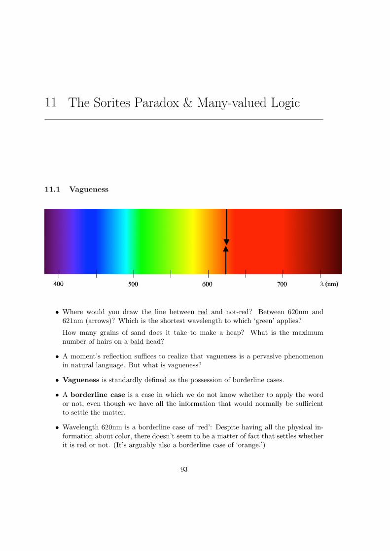
11 The Sorites Paradox & Many-valued Logic
11.1 Vagueness
• Where would you draw the line between red and not-red? Between 620nm and621nm (arrows)? Which is the shortest wavelength to which ‘green’ applies?
How many grains of sand does it take to make a heap? What is the maximumnumber of hairs on a bald head?
• A moment’s reflection suffices to realize that vagueness is a pervasive phenomenonin natural language. But what is vagueness?
• Vagueness is standardly defined as the possession of borderline cases.
• A borderline case is a case in which we do not know whether to apply the wordor not, even though we have all the information that would normally be sufficientto settle the matter.
• Wavelength 620nm is a borderline case of ‘red’: Despite having all the physical in-formation about color, there doesn’t seem to be a matter of fact that settles whetherit is red or not. (It’s arguably also a borderline case of ‘orange.’)
93
94 The Sorites Paradox & Many-valued Logic
Contrast this with wavelengths 680nm and 500nm: 680nm is clearly red, 500nmclearly not red.
• Is vagueness a feature of the meaning of natural languages? Or is it a feature of theworld? Are there vague objects?
11.1.1 What Vagueness is Not
1. Vagueness individuals’ linguistic incompetence:
Experts tell us that the visible color spectrum is continuous, with no sharp bound-aries between one color and the next. Are we all incompetent? This would cry foran explanation.
2. Vagueness ambiguity:
Lexical ambiguity:1 individual words have more than one meaning in the languageto which they belong (where ‘meaning’ refers to what could be captured by a diction-ary).2 Some clear cases: bank, bill, stage, still. . . Consider an ambiguous adjective:
(11.1) The storm was terrific.
Even after clarifying the intended meaning of ‘terrific’ in an utterance of (11.1),vagueness remains: there are borderline cases of ‘terrible/frightening’ as well as of‘marvelous/wonderful.’
3. Vagueness & context-sensitivity: vagueness does not reduce to dependence on thecomparison class picked out in the context of use.
Consider Danny, who is 1,75m in height. Is Danny tall?
(11.2) Context: Danny’s dad is talking to other dads about how fast her12year-old son Danny has been growing recently.
Glen: Danny is tall.Paul: That’s right! He’s been growing so fast since he turned 12 in the fall.
(11.3) Context: Danny’s mom is talking to other moms about NBA basketball.
Sue: Danny isn’t tall. He’s very talented but just wouldn’t stand a chance againstthose guys.
Why do both Glen’s use of ‘Danny is tall’ in his context and Sue’s use of ‘Dannyisn’t tall’ in her context seem true? What is said with a comparative adjective incontext depends on the comparison class implicitly referred to in context (Kennedy,
1Contrast lexical ambiguity with structural ambiguity; e.g. ‘Visiting relatives can be boring’, ‘He sawthat gasoline can explode’ [(a) He saw an explosion of a can of gasoline, (b) He recognized the fact thatgasoline is explosive]
2Not all variation in word-meaning is ambiguity. A defeasible test is as follows: For a given word Wthat has more than one meaning, if there is another natural language that has different words for thosemeanings, this is positive evidence for W ’s being ambiguous.
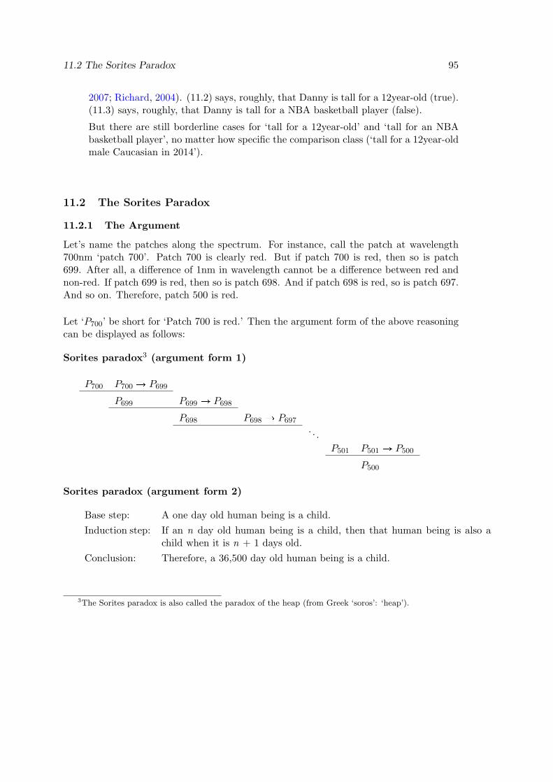
11.2 The Sorites Paradox 95
2007; Richard, 2004). (11.2) says, roughly, that Danny is tall for a 12year-old (true).(11.3) says, roughly, that Danny is tall for a NBA basketball player (false).
But there are still borderline cases for ‘tall for a 12year-old’ and ‘tall for an NBAbasketball player’, no matter how specific the comparison class (‘tall for a 12year-oldmale Caucasian in 2014’).
11.2 The Sorites Paradox
11.2.1 The Argument
Let’s name the patches along the spectrum. For instance, call the patch at wavelength700nm ‘patch 700’. Patch 700 is clearly red. But if patch 700 is red, then so is patch699. After all, a difference of 1nm in wavelength cannot be a difference between red andnon-red. If patch 699 is red, then so is patch 698. And if patch 698 is red, so is patch 697.And so on. Therefore, patch 500 is red.
Let ‘P700’ be short for ‘Patch 700 is red.’ Then the argument form of the above reasoningcan be displayed as follows:
Sorites paradox3 (argument form 1)
P700 P700 Ñ P699
P699 P699 Ñ P698
P698 P698 Ñ P697
. . .
P501 P501 Ñ P500
P500
Sorites paradox (argument form 2)
Base step: A one day old human being is a child.
Induction step: If an n day old human being is a child, then that human being is also achild when it is n + 1 days old.
Conclusion: Therefore, a 36,500 day old human being is a child.
3The Sorites paradox is also called the paradox of the heap (from Greek ‘soros’: ‘heap’).
96 The Sorites Paradox & Many-valued Logic
11.2.2 Responses to the Sorites Paradox
• A paradox is an apparently valid argument which has apparently true premises butwhich has an absurd consequence.
• Argument form 1: P700 seems clearly true. XThe P700 Ñ P699 is also extremely plausible and so true. XP699 follows from the above by deductive reasoning. X
...But the conclusion, P500, is clearly false. Paradox
• Why is the conditional plausible?
Tolerance Vague expressions are tolerant: small changes do not affect the applicabilityof the word. For instance, if two color patches are indistinguishable in color,then both or neither are red.
• Ways of resolving a paradox:
1. Reject one or more of the premises
Epistemicism (Sorensen, 1988; Williamson, 1994)Supervaluationism (van Fraassen, 1966; Kamp, 1975; Fine, 1975; Keefe,2000)
2. Reject the reasoning as defective (e.g., invalid)
Many-valued logic and degrees of truth ( L ukasiewicz and Tarski, 1930;Zadeh, 1965)Contextualism (Raffman, 1996; Soames, 1999; Shapiro, 2006)4
3. Bite the bullet and accept the conclusion
Vague concepts are flawed. (Unger, 1979)
• Accept the conclusion: Unger’s view
Sorites paradoxes show that vague concepts are deeply flawed: they commit us toabsurdities. They are a flawed way to cut up the world. Flawed concepts are onesunder which nothing can fall. So even if the world is full of stuff, there are no heaps,bald people, red things, mountains, etc.
• Reject a premise: Epistemicism
– Vagueness is nothing but ignorance. Vague expressions have precise meanings:they cut the world along its sharp boundaries (the heaps are separated fromthe non-heaps by a sharp line). But we fail to know where those boundariesfall. Why? Our cognitive mechanisms require a margin for error to deliverknowledge. But even if I believe truly that patch 620 is red and patch 619 isnot, I do not know this: for all I know, the concept I employ could be red*,whose boundary is between wavelengths 620nm and 621nm.
4A good overview of contextualism can be found in Akerman and Greenough (2010).
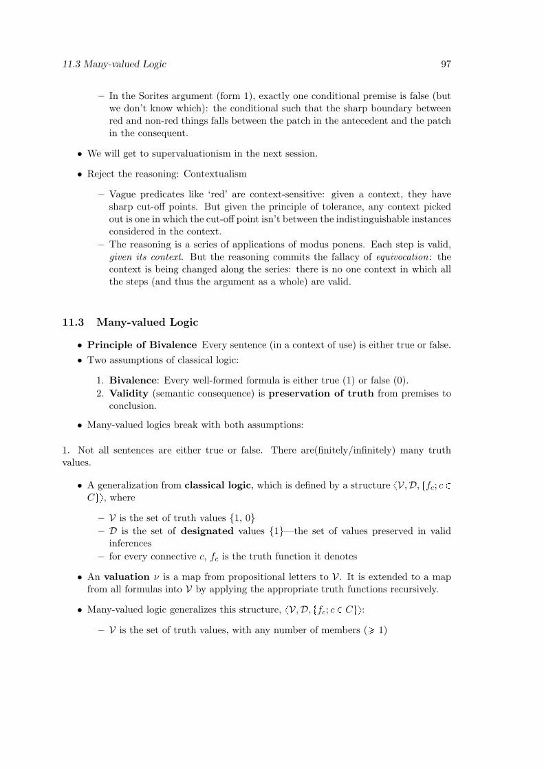
11.3 Many-valued Logic 97
– In the Sorites argument (form 1), exactly one conditional premise is false (butwe don’t know which): the conditional such that the sharp boundary betweenred and non-red things falls between the patch in the antecedent and the patchin the consequent.
• We will get to supervaluationism in the next session.
• Reject the reasoning: Contextualism
– Vague predicates like ‘red’ are context-sensitive: given a context, they havesharp cut-off points. But given the principle of tolerance, any context pickedout is one in which the cut-off point isn’t between the indistinguishable instancesconsidered in the context.
– The reasoning is a series of applications of modus ponens. Each step is valid,given its context. But the reasoning commits the fallacy of equivocation: thecontext is being changed along the series: there is no one context in which allthe steps (and thus the argument as a whole) are valid.
11.3 Many-valued Logic
• Principle of Bivalence Every sentence (in a context of use) is either true or false.
• Two assumptions of classical logic:
1. Bivalence: Every well-formed formula is either true (1) or false (0).
2. Validity (semantic consequence) is preservation of truth from premises toconclusion.
• Many-valued logics break with both assumptions:
1. Not all sentences are either true or false. There are(finitely/infinitely) many truthvalues.
• A generalization from classical logic, which is defined by a structure xV,D, tfc; c PCuy, where
– V is the set of truth values 1, 0– D is the set of designated values 1—the set of values preserved in valid
inferences
– for every connective c, fc is the truth function it denotes
• An valuation ν is a map from propositional letters to V. It is extended to a mapfrom all formulas into V by applying the appropriate truth functions recursively.
• Many-valued logic generalizes this structure, xV,D, tfc; c P Cuy:
– V is the set of truth values, with any number of members (¥ 1)
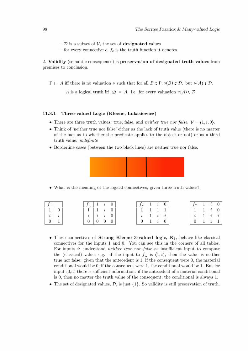
98 The Sorites Paradox & Many-valued Logic
– D is a subset of V, the set of designated values
– for every connective c, fc is the truth function it denotes
2. Validity (semantic consequence) is preservation of designated truth values frompremises to conclusion.
Γ ( A iff there is no valuation ν such that for all B P Γ, νpBq P D, but νpAq R D.
A is a logical truth iff H ( A, i.e. for every valuation νpAq P D.
11.3.1 Three-valued Logic (Kleene, Lukasiewicz)
• There are three truth values: true, false, and neither true nor false. V t1, i, 0u.• Think of ‘neither true nor false’ either as the lack of truth value (there is no matter
of the fact as to whether the predicate applies to the object or not) or as a thirdtruth value: indefinite
• Borderline cases (between the two black lines) are neither true nor false.
• What is the meaning of the logical connectives, given three truth values?
f 1 0i i0 1
f^ 1 i 0
1 1 i 0i i i 00 0 0 0
f_ 1 i 0
1 1 1 1i 1 i i0 1 i 0
f 1 i 0
1 1 i 0i 1 i i0 1 1 1
• These connectives of Strong Kleene 3-valued logic, K3, behave like classicalconnectives for the inputs 1 and 0. You can see this in the corners of all tables.For inputs i: understand neither true nor false as insufficient input to computethe (classical) value; e.g. if the input to f is x1, iy, then the value is neithertrue nor false: given that the antecedent is 1, if the consequent were 0, the materialconditional would be 0; if the consequent were 1, the conditional would be 1. But forinput x0,iy, there is sufficient information: if the antecedent of a material conditionalis 0, then no matter the truth value of the consequent, the conditional is always 1.
• The set of designated values, D, is just 1. So validity is still preservation of truth.
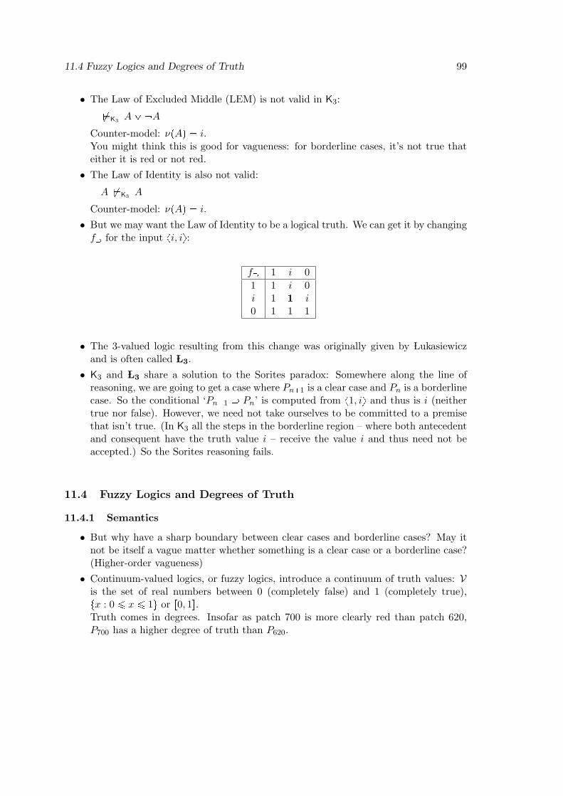
11.4 Fuzzy Logics and Degrees of Truth 99
• The Law of Excluded Middle (LEM) is not valid in K3:
*K3A_ A
Counter-model: νpAq i.You might think this is good for vagueness: for borderline cases, it’s not true thateither it is red or not red.
• The Law of Identity is also not valid:
A *K3A
Counter-model: νpAq i.
• But we may want the Law of Identity to be a logical truth. We can get it by changingf for the input xi, iy:
f 1 i 0
1 1 i 0i 1 1 i0 1 1 1
• The 3-valued logic resulting from this change was originally given by Lukasiewiczand is often called L3.
• K3 and L3 share a solution to the Sorites paradox: Somewhere along the line ofreasoning, we are going to get a case where Pn1 is a clear case and Pn is a borderlinecase. So the conditional ‘Pn1 Pn’ is computed from x1, iy and thus is i (neithertrue nor false). However, we need not take ourselves to be committed to a premisethat isn’t true. (In K3 all the steps in the borderline region – where both antecedentand consequent have the truth value i – receive the value i and thus need not beaccepted.) So the Sorites reasoning fails.
11.4 Fuzzy Logics and Degrees of Truth
11.4.1 Semantics
• But why have a sharp boundary between clear cases and borderline cases? May itnot be itself a vague matter whether something is a clear case or a borderline case?(Higher-order vagueness)
• Continuum-valued logics, or fuzzy logics, introduce a continuum of truth values: Vis the set of real numbers between 0 (completely false) and 1 (completely true),tx : 0 ¤ x ¤ 1u or r0, 1s.Truth comes in degrees. Insofar as patch 700 is more clearly red than patch 620,P700 has a higher degree of truth than P620.
100 The Sorites Paradox & Many-valued Logic
• The meaning of the connectives:
f pxq 1 x
f^px, yq Minpx, yq
f_px, yq Max px, yq
fÑpx, yq xa y
where Min means ‘the minimum (lesser) of; Max means ‘the maximum (greater) of’;and xa y is a function defined as follows:
if x ¤ y, then xa y 1
if x ¡ y, then xa y 1 px yq p 1 x yq
• So as the truth value of a formula does down, the truth value of its negation goes up.A conjunction is as true as its least true conjunct. A disjunction is as true as its mosttrue disjunct. For the conditional: If we reason from an antecedent to a consequentthat has more truth than the antecedent, that’s good reasoning; it receives 1. Whatif we reason from an antecedent to a consequent less true? That’s less than perfect.How much less? That depends on the difference in truth between antecedent andconsequent. The truth of the conditional goes down proportionally to the drop indegree of truth from antecedent to consequent.
• Note that for truth values 1 and 0, the truth functions behave just like the classicalones. And for the truth value 0.5, the truth functions behave just like i in L3. Theresulting logic, L, is a generalization of Lukasiewicz’s 3-valued logic.
• Validity: What are the designated values in L? We could say that the only des-ignated value is 1. But then we get valid reasoning as soon as a single premise isless than completely true. So what about all the values greater than 0.75? Butthis seems random. Why 0.75 and not 0.7 or 0.8? The important idea is this: Aninference is valid iff under any valuation the conclusion is at least as true as the leasttrue premise. That is, it isn’t less true than the least true premise.
For any set of truth values, there will always be a number that is less than or equalto every number in the set. For the set X : t0.21, 0.201, 0.2001, 0.20001, . . .u, thisnumber is 0.2. Call it the greatest lower bound of X, GlbpXq.
Let νrΓs be tνpBq : B P Γu. Then
Γ ( L A iff for all ν, GlbpνrΓsq ¤ νpAq
11.4.2 Fuzzy Logic and the Sorites Paradox: Reject Modus Ponens
• Modus Ponens (MP) is not valid in L: A,AÑ B * L B
It’s true that if the premises all take truth value 1, so does the conclusion. Butconsider a valuation ν that assigns A a greater degree of truth than B; e.g. νpAq
11.5 Readings 101
0.9 and νpBq 0.8. Then the conditional takes the truth value 1 0.9 0.8 0.9.So the minimum degree of truth of the premises is 0.9. But the conclusion is trueonly to degree 0.8. Hence, it’s not the case that the conclusion is at least as true asthe least true premise.
• The failure of Modus Ponens is also responsible for the invalidity of the Sorites ar-gument: Take an arbitrary application of MP in the Sorites series, e.g. P651, P651 ÑP650 ñ P650. Suppose νpP651q 0.651 and νpP650q 0.650. Then νpP651 Ñ P650q 0.999. So the least true premise has truth value 0.651. However, the conclusion hasthe lower truth value 0.650. So this step in the series is not valid, and thus theargument as a whole isn’t.
11.5 Readings
• Priest (2008, §§7.1–7.4) on many-valued logics
Sainsbury (1995, 40-47) on the Sorites paradox
• Optional: Priest (2008, §§11.1-11.4) on fuzzy logics
Williamson (1994, §§4.1–4.6) on many-valued and fuzzy logics


12 Supervaluationism
To be written. . .
103

Bibliography
Adams, E. W. (1970). Subjunctive and indicative conditionals. Foundations of Lan-guage 6 (1), 89–94.
Akerman, J. and P. Greenough (2010). Vagueness and non-indexical contextualism. InS. Sawyer (Ed.), New Waves in Philosophy of Language. New York: Palgrave Macmillan.
Bell, J. L., D. DeVidi, and G. Solomon (2001). Logical Options. An Introduction toClassical and Alternative Logics. Peterborough: Broadview Press.
Bennett, J. (2003, June). A Philosophical Guide to Conditionals. New York and Oxford.Oxford University Press.
Edgington, D. (1995). On conditionals. Mind 104 (414), 235–329.Fine, K. (1975). Vagueness, truth and logic. Synthese 30 (3/4), 265–300.Gibbard, A. (1981). Two recent theories of conditionals. In W. Harper, R. Stalnaker, and
G. Pearce (Eds.), Ifs: Conditionals, Belief, Decision, Chance, and Time, pp. 211–47.Dordrecht: Reidel.
Grice, H. P. (1975). Logic and conversation. In P. Cole and J. Morgan (Eds.), Syntaxand Semantics 3: Speech Acts, pp. 41–58. Page references are to the reprint in Grice(1989b), pp. 22–40. New York: Academic Press.
Grice, H. P. (1989a). Indicative conditionals. In Studies in the Way of Words, pp. 58–85.Cambridge, MA: Harvard University Press.
Grice, H. P. (1989b). Studies in the Way of Words. Cambridge, MA, and London: HarvardUniversity Press.
Higginbotham, J. (1986). Linguistic theory and davidson’s program in semantics. InE. LePore (Ed.), Truth and Interpretation: Perspectives on the Philosophy of DonaldDavidson, pp. 29—48. Oxford: Blackwell.
Jackson, F. (1979). On assertion and indicative conditionals. The Philosophical Re-view 88 (4), 565–89.
Kamp, H. (1975). Two theories about adjectives. In E. Keenan (Ed.), Formal Semanticsof Natural Language. Cambridge: Cambridge University Press.
Keefe, R. (2000). Theories of Vagueness. Cambridge: Cambridge University Press.Kennedy, C. (2007). Vagueness and grammar: The semantics of relative and absolute
gradable adjectives. Linguistics and Philosophy 30 (1), 1–45. L ukasiewicz, J. and A. Tarski (1930). Untersuchungen uber den aussagenkalkul. Comptesrendus des seances de la Societe des Sciences et des Lettres de Varsovie 3 (23), 12–21,
105
106 BIBLIOGRAPHY
30–50. Translated into English by J.H. Woodger as ‘Investigations into the SententialCalculus,’ in Corcoran, J .(ed), Logic, Semantics, Metamathematics, 2nd ed., Indiana-polis: Hackett, 1983.
Lewis, C. I. (1917). The issues concerning material implication. Journal of Philosophy,Psychology and Scientific Methods 14 (13), 350–56.
Lewis, D. (1973). Counterfactuals. Oxford: Blackwell.Lowe, E. (2002). A Survey of Metaphysics. Oxford: Oxford University Press.Portner, P. (2009). Modality. Oxford: Oxford University Press.Priest, G. (2008). An Introduction to Non-Classical Logic. From If to Is (2nd ed.). Cam-
bridge: Cambridge University Press.Raffman, D. (1996). Vagueness and context-relativity. Philosophical Studies 81 (2-3),
175–92.Ramsey, F. P. (1931). General propositions and causality. In The Foundations of Math-
ematics, pp. 237–55. London: Kegan Paul.Read, S. (1994). Thinking About Logic. Oxford: Oxford University Press.Richard, M. (2004). Contextualism and relativism. Philosophical Studies 119 (1), 215–42.Sainsbury, R. (1995). Paradoxes (3rd ed.). Cambridge: Cambridge University Press.Shapiro, S. (2006). Vagueness in Context. Oxford: Oxford University Press.Sider, T. (2010). Logic for Philosophy. Oxford: Oxford University Press.Soames, S. (1999). Understanding Truth. New York, Oxford: Oxford University Press.Sorensen, R. (1988). Blindspots. Oxford: Clarendon Press.Stalnaker, R. C. (1968). A theory of conditionals. In N. Rescher (Ed.), Studies in Logical
Theory, pp. 98–112. Oxford: Blackwell.Stalnaker, R. C. (1975). Indicative conditionals. Philosophia 5 (3), 269–86; page references
are to the reprint in Stalnaker (1999).Stalnaker, R. C. (1978). Assertion. In P. Cole (Ed.), Syntax and Semantics 9: Pragmatics,
pp. 315–32; page references are to the reprint in Stalnaker (1999). New York: AcademicPress.
Stalnaker, R. C. (1999). Context and Content. Oxford: Oxford University Press.Unger, P. (1979). There are no ordinary things. Synthese 41, 117–54.van Fraassen, B. C. (1966). Singular terms, truth-value gaps, and free logic. Journal of
Philosophy 53, 481–5.von Fintel, K. (2006). Modality and language. In D. Borchert (Ed.), Encyclopedia of
Philosophy (2nd ed.). Detroit: Macmillan Reference.von Fintel, K. (2011). Conditionals. In K. von Heusinger, C. Maienborn, and P. Portner
(Eds.), Semantics: An International Handbook of Natural Language Meaning, Volume 2.Berlin and New York: de Gruyter.
Williamson, T. (1994). Vagueness. London: Routledge.Williamson, T. (1998). Bare possibilia. Erkenntnis 48 (2-3), 257–73.Zadeh, L. (1965). Fuzzy sets. Information and Control 8, 338–53.