Phenotypic variation in past and present Scandinavian wolves (Canis lupus L.)

Vilde Arntzen Engdal

Master Thesis (60 credits) Ecology and evolution

Department of Biosciences

Faculty of Mathematics and Natural Sciences

UNIVERSITY OF OSLO

December 2018

II

III

© Vilde Arntzen Engdal

2018

Phenotypic variation in past and present Scandinavian wolves (Canis lupus L.)

Author: Vilde Arntzen Engdal

http://www.duo.uio.no/

Print: Reprosentralen, Universitetet i Oslo

IV

V

Acknowledgements This study would not have been feasible without the dedicated help and assistance of a

number of people and institutions. Undoubtedly, the most challenging situations arose when

trying to cover as many square kilometers and wolves as possible during the most intensive

periods of field work. The dedicated hunters in the Brattfors, Loka, Blyberget, Julussa and

Osdalen territories are thanked for their willingness to provide access to their quarries, and

their general kind patience with us useless research types. A special thanks goes to Martin

Monné and Erling Nordgaard for access to their vast network of contacts and co-ordinating

roles on the Norwegian side. On the Swedish side, the resourcefulness and logistical support

of Phil. Cand. Mattias Widstrand and his company Köla Skogservice was absolutely essential

to not only endure but even navigate and work in the most desolate and remote hinterlands of

Swedish forest imaginable. How on Earth it is possible to keep such amounts of knowledge

about terrain, backroads, rendezvous points, territorial borders, the general natural

environment and whatnot within the confines of one human brain remains a mystery. Most

importantly, I will always share your devotion to the forest and all living things in it.

Professor Øystein Wiig and curator Daniella Kalthoff at the Oslo and Stockholm museums of

natural history are heartfully thanked for their assistance and providing access to their

respective collections. A special thanks goes to Peter Mortensen in Stockholm for assembling

metadata on the available specimens. Kaj Granlund is thanked for providing the background

reference for the morphological measurements and for his relentless enthusiasm for

documenting what past and presents wolves actually look like. A big thanks to my supervisor

at UiO Glenn-Petter Sætre for your confidence and giving me the freedom to freely explore

this rather unusual topic. To my supervisor at NMBU, Øyvnid Øverli a huge thanks for all the

time you have invested in this project and for giving me the opportunity. I have appreciated

all the help you have provided, all the field trips to the deep Scandinavian forests and the

good conversations we have had. This thesis would not have been possible without your

relentless commitment to the scientific prosses. Maren Høyland, Marco Vindas and Christina

Sørensen are thanked for their essential advise on statistical intricacies and comments on

various stages of the writing of this thesis. To my Family, thanks for all the support and love

you have provided during this process. To Nicolai Aasen, for being there every step of the

way, for the love and support, and for all the late evenings you have accompanied during

hectic field expeditions. And last but not least, thanks to my own canid, Piaf.

VI

VII

Abstract During the last century, the grey wolf (Canis lupus L.) was subject to extensive hunting

pressure, which led to functional extinction of this species from the Scandinavian Peninsula

around 1970. Wolves reappeared in Scandinavia in 1983 when one male and one female wolf

established a territory at the border between southern Sweden and Norway. One new male

contributed to the population in 1991, and these three individuals are considered the

functional founders of the present wolf population in Scandinavia. The extant wolf population

has been subject to numerous studies of pedigree, genetic variability and dispersal. Systematic

documentation and studies of morphology have been called for, but are scarce. Also, few

studies have investigated morphological differences between the extinct and extant

Scandinavian wolf population. Available material from both populations consist of skulls and

preserved hides in museum collections. In this thesis, skull measurements and size of foreleg

melanin patches were compared between the two populations. Further, standardized

photographic documentation and anatomical measures were obtained from recently shot

wolves (n=35) during licensed hunts in Scandinavia in 2017 and 2018. This material was used

to achieve redundant control for possible confounding factors in the museum material

regarding size of melanin markings. The extinct wolf population (museum material, n=12)

carried significantly larger foreleg markings than the extant population (n=72) overall. There

were no significant effects of sex in either field or museum specimens, but in the field

material juveniles had significantly larger melanin patches than adults. Frequencies of males

vs juveniles were equally distributed between the extant and extinct fractions of the museum

material. The field data further indicated that leg length did not affect the size of foreleg

marks. A principal component analysis was performed on 16 craniometric variables obtained

from adult males from the extinct (n=11) and extant (n=47) population. Separation of the

populations was indicated for the 1st and 3rd PC axis. The most contributing variables to PC1

and PC3 was Condylobasal length (CbL) and forehead slope (Fs), respectively. The study

populations significantly differed in both these variables, indicating a longer and flatter skull

in extant compared to extinct wolves. Possible explanations for the observed morphological

differences could be variation in geographical origin, adaptation to different environments,

differences in available nutrients, or simply random founder effects followed by inbreeding.

Further research should be carried out in order to understand the genotype-phenotype

interaction underlying the differences in morphology between past and present wolves.

VIII

IX

Contents 1 Introduction ........................................................................................................................ 1

1.1 Morphological plasticity in Canids ............................................................................ 1

1.2 The grey wolf ............................................................................................................. 2

1.3 The grey wolf in Scandinavia: Why phenotypes matter ............................................ 3

1.4 A note on available study material ............................................................................. 4

1.5 Color variation, with a particular note on melanin patches ........................................ 5

1.6 Aims and rationale ..................................................................................................... 7

2 Material and Methods ......................................................................................................... 8

2.1 Study material ............................................................................................................ 8

2.1.1 Field work .......................................................................................................... 8

2.1.2 Museum collections ............................................................................................ 9

2.2 Data collection .......................................................................................................... 10

2.2.1 Photography ..................................................................................................... 10

2.2.2 Field morphometry ........................................................................................... 12

2.2.3 Skulls morphometry ......................................................................................... 14

2.3 Photograph processing ............................................................................................. 16

2.3.1 Foreleg mark .................................................................................................... 16

2.4 Statistical analysis .................................................................................................... 17

2.4.1 Craniometrics ................................................................................................... 17

2.4.2 Foreleg mark .................................................................................................... 18

3 Results .............................................................................................................................. 19

3.1 Skull morphometry in in the extinct and extant Scandinavian wolf population ...... 19

3.2 Foreleg mark size ..................................................................................................... 27

4 Discussion ........................................................................................................................ 32

4.1 Methodical considerations ........................................................................................ 32

4.2 The natural history of the grey wolf in Scandinavia ................................................ 33

4.3 Results in brief ......................................................................................................... 34

4.4 Skull morphology ..................................................................................................... 35

4.5 Foreleg melanin patches ........................................................................................... 38

5 Conclusions ...................................................................................................................... 42

6 References ........................................................................................................................ 43

X

Appendix .................................................................................................................................. 49

1

1 Introduction

1.1 Morphological plasticity in Canids

Presently represented by over 10 genera and more than 30 species, the Canidae are both the

most widely distributed family of carnivores and one of the earliest originating extant group

of this order. Canids and their biology fascinate both specialists and laymen, due to a range of

attributes from their physical and cognitive abilities to their often highly complex and

structured social behavior. Undoubtedly, our relationship with domestic dogs which probably

dates back more than 14.000 years (Driscoll et al., 2009) contributes to this allure. Conjointly

intriguing is the inherent capacity of many canids to generate both heritable phenotypic

variation (“evolvability”) and rapid responses to the environment. (Radinsky, 1973; Fondon

& Garner, 2004; Van Valkenburgh, 2007; Curtis et al., 2018)

Like domestic dogs, wild canids exhibit great morphological variation, from the small

fennec fox (Vulpes zerda, shoulder height: 15-20 cm), to the long-legged maned wolf

(Chrysocyon brachyurus, shoulder height: 74-91 cm) (Castelló, 2018). Morphological

variation reflects the variety in predatory strategies and dietary preferences found in the

Canidae family (Slater et al., 2009). The diet of canid species can vary from hypercarnivores,

omnivores, where half the diet consist of fruit, to insectivores like the bat-eared fox (Otocyon

megalotis megalotis) (Slater et al., 2009; Asahara, 2013). One feature that distinguishes the

family of Canidae from the rest of the carnivoran families is that they show higher flexibility

and evolvability particularly in skull traits, such as higher flexibility in facial length and nasal

length (Machado et al., 2018). Even though canids exhibit a wide range of predatory

strategies, prey apprehension mostly rely on their teeth and skull (Slater et al., 2009). High

flexibility and evolvability in these traits may allow canids to respond to selective pressure

such as shifts in prey availability (Machado et al., 2018). Shorter snout and broader jaws are

associated with greater bite force and the ability to take down large prey, while narrow and

long faces are associated with fast-closing jaws, specialized in catching small animals (Slater

et al., 2009).

2

The grey wolf (Canis lupus) was the first animal to become domesticated by humans, a

process that started > 14,000 year ago, and resulted in the morphological diverse species

known as man’s best friend, the domestic dog (Canis lupus familiaris) (Driscoll et al., 2009).

Domestic dogs displays the greatest morphological diversity found among terrestrial

mammalian species (Schoenebeck & Ostrander, 2013). Variation in body proportions and size

in domestic dog exceed the variation found among the wild canids (Wayne, 1986), and the

variation in domestic dogs skull morphology is comparable to skull variation found in the

entire Carnivoran order (Drake & Klingenberg, 2010).

A study conducted by Laidlaw et al. (2007) looked at the tandem repeat length

variation in the genome of dogs and other carnivoran clades as a source of morphological

variation. These authors found that wild and domestic canids possess an elevated occurrence

of pure repetitive sequences that surpass those of other carnivoran clades (Laidlaw et al.,

2007). Furthermore, domestic dogs have a genome-wide high slippage mutation rate, a

character derived from their ancestors before domestication which has been preserved in

modern wild canids. This may explain the high and quickly developing phenotypic variation

found in both wild and domestic canids (Laidlaw et al., 2007; Machado et al., 2018). This

distinctive quality makes wolves (Canis lupus) an interesting species for studying

morphological changes through biological events in the wild, such as genetic bottlenecks,

geographical dispersal, and environmental change.

1.2 The grey wolf

The largest member of the wild canids is the Grey wolf (Canis lupus) (Castelló, 2018).

Historically, wolves were once the most widely distributed terrestrial mammal found

throughout the Northern hemisphere (Mech, 1995). They are great dispersers and inhabit a

range of different habitats like arctic tundra, deserts, grassland, mountains, woodland and

prairies where they primarily prey on ungulates (Mech & Boitani, 2003; Geffen et al., 2004).

Wolves are today no longer the most widely distributed terrestrial mammal, as they suffered

persecution by humans on a global scale (Fritts et al., 2003). With the expansion of human

settlement, competition for wild ungulates and fragmentation of habitats, large predators

encountered conflicts with humans and their livestock (Delibes, 1990; Breitenmoser, 1998).

Together with the rapid development of firearms, wildlife traps and the use of poison over the

last two centuries, large predators were pursued and killed in high numbers (Pimlott, 1973;

3

Delibes, 1990; Mech, 1995; Wabakken et al., 2001). Wolves were especially targeted, and

many European countries set out to exterminate the species (Boitani, 1995; Fritts et al., 2003).

As a consequence, wolf populations reached critical low numbers around 1930-1960 and

disappeared from many European countries (Delibes, 1990; Mech, 1995). The remaining

populations were fragmented and isolated in small groups until the species became protected

(Boitani, 2003; Pilot et al., 2014). After 1980, wolf populations started to expand and

recolonize (Boitani, 2003). Many of the European wolf populations experienced severe

genetic and demographic bottlenecks as a consequence of persecution of the species; this

includes the Italian population, the Scandinavian population and the eastern and western

Balkan populations to mention some (Vila et al., 2003; Fabbri et al., 2007; Djan et al., 2014).

1.3 The grey wolf in Scandinavia: Why phenotypes matter

Scandinavia followed the same trend as the rest of Europe. In Norway, a law of eradication of

predators was sanctioned in 1845, which included bounties for many of the large predators

(Bjerve, 1978). Similar events took place in Sweden and wolves were actively hunted until

the species became legally protected in 1966 in Sweden and 1972 in Norway (Haglund, 1973;

Delibes, 1990; Wabakken et al., 2001). By this time only a few individuals were observed on

the Scandinavian peninsula, and the population became functionally extinct (Haglund, 1973;

Wabakken et al., 2001).

In 1980, a sighting of wolves was reported in Scandinavia and in 1983 two wolves

successfully reproduced in Värmland, Sweden, and continued reproducing in the following

years (Delibes, 1990; Wabakken et al., 2001). In 1991 a new non-related male successfully

reproduced, followed by two new males in 2008 (Jansson et al., 2015). These five individuals,

one female and four males, are the founders of the new population in Scandinavia, and the

three first individuals contribute over 95% of the present gene pool (Jansson et al., 2015).

Today the Scandinavian wolf population is estimated to be around 400 individuals (2017-

2018) mainly distributed in central Scandinavia with the majority of the population found in

Sweden and one-quarter of the population found in Norway close to the Swedish border

(Wabakken et al., 2018). The number of breeding pairs and the geographical distribution of

their territories is today governmentally controlled by legal hunting with a collaboration

between the countries (Wabakken et al., 2018). The newly immigrated wolves in Denmark

4

should not be viewed as part of the Scandinavian population as these individuals stem from

immigrating wolves from Germany/Poland (Andersen et al., 2015) and no gene flow between

the two populations occurs.

The extant Scandinavian wolf population is closely monitored, and the population’s pedigree

is almost complete (Åkesson et al., 2016). Many studies have been conducted on genetic

variability in the Scandinavian population and the risk for inbreeding depression (Vila et al.,

2003; Liberg et al., 2005; Åkesson et al., 2016; Kardos et al., 2018). A study concerning

genomic consequences of inbreeding by Kardos et al. (2018) found that many individuals in

the severe inbred Scandinavian population have entire or nearly entire chromosomes that are

homozygous. This study concluded that further studies should investigate the phenotypic

consequences for the inbred population. To my knowledge only two such studies have been

carried out, one investigating fluctuating asymmetry in skull traits of the extinct and extant

populations (Wiig & Bachmann, 2014), and one examining malformations of the backbone in

wolves from Finland and the extinct and extant Scandinavian populations (Räikkönen et al.,

2006). Only the latter found indications of phenotypic consequences of inbreeding depression

in the extant population. With these notable exceptions, compared to the extensive research

on wolves and all aspects of their biology elsewhere (especially in North-America) (Musiani

et al., 2007; Wheeldon & Patterson, 2012; O'Keefe et al., 2013), systematic registration of

phenotypic variation in both the extant and extinct Scandinavian wolves can only be

described as profoundly lacking. In an attempt to initiate more integrative studies, this thesis

aims to further investigate and document morphological traits in the extant Scandinavian wolf

population and compare trait variability in the extant population to the historical extinct

Scandinavian wolf population.

1.4 A note on available study material

With the time and financial resources available to this MSc thesis, available study material

was largely limited to collections at the natural history museums of Oslo and Stockholm.

These collections consist of skulls and (from a lower number of individuals) preserved hides

obtained in the period from 1830 - 2018. Hence, skull morphology and to a limited degree

coat color variation can be compared between the study populations. In addition, I was able to

obtain standardized photographic documentation and anatomical measures from recently shot

wolves (whole bodies) during licensed hunts in Norway and Sweden during the winters of

5

2017 and 2018. This material is used to achieve redundant control for a possible confounding

factor in the museum material, namely the lack of information about actual body size and its

possible relationship to the size of melanin-based color patches (see below). While the

ultimate goal would be to conduct studies linking genotype and phenotype, here I am limited

to analyze and present only phenotypic variability in the study material.

1.5 Color variation, with a particular note on melanin patches

Variation in animal pigmentation has spurred and provided key models some of the most

active and controversial fields in evolutionary biology including sexual selection,

aposematism, crypsis and mimicry (Hamilton & Zuk, 1982; Majerus, 1998; McGraw & Hill,

2000; Sherratt & Beatty, 2003; Hoekstra, 2006; Gray & McKinnon, 2007) Furthermore, color

polymorphisms provide the sort of raw material widely thought to facilitate sympatric

speciation (Sinervo & Svensson, 2002; Bolnick & Fitzpatrick, 2007; Gray & McKinnon,

2007; Fitzpatrick et al., 2009). In vertebrates, two main pigment groups, carotenoids and

melanins, cause color variation. Variation in carotenoid pigmentation is mostly condition-

dependent and is assumed to signal individual “quality”, in the sense that carotenoids are in

limited supply and also have other critical functions (mainly in antioxidative processes and

immune responses) than ornamentation (von Schantz et al., 1999; Clotfelter et al., 2007;

Vinkler & Albrecht, 2010). In contrast, stable (and often heritable) color polymorphisms most

often involve genes responsible for synthesis and deposition of melanin – in vertebrates the

black pigment eumelanin, and red to brownish phaeomelanin (Alexandre Roulin, 2004;

McKinnon & Pierotti, 2010).

Grey wolves can possess a range of different color morphs, from mono-colored fur in black or

white to color pallets in grey, ochre, tawny and brown (Pocock, 1935). The most common fur

morph is a variation of grey coat color and is common for the Eurasian subspecies, which the

Scandinavian population is considered a part of (Pocock, 1935; Sillero-Zubiri et al., 2004).

One striking coat color feature described in many of the subspecies of grey wolfs is a black

stripe running down the front of the foreleg (Pocock, 1935; Ognev, 1962; Castelló, 2018).

Due to technical difficulties with quantifying hue and intensity of other colors, I constrained

the efforts within this thesis to develop a method to capture variation in this melanin-based

marking.

6

I include these data since melanin-based coloration have also been associated with other

phenotypic traits and the existence of behavioral syndromes in several vertebrates. Typically,

individuals with pronounced melanin markings are found to be generally more aggressive,

sexually active and resistant to stress and infection (Ducrest et al., 2008; Kittilsen et al., 2009;

Kittilsen et al., 2012). Notably, in those species where dark hues or patterns are not used for

camouflage, contrast-rich black patches are often major characteristics of life-history strategy,

and are presumed to act as a social signal (Järvi & Bakken, 1984; Horth, 2003; Alexandre

Roulin et al., 2008). Well documented examples are the breast stripe of the male great tit

(Parus major), which is wider in socially dominant individuals, and the lion’s (Panthera leo)

mane, which is darker in successful pride leading males.

In some cases, such as in the lions, this co-variation is highly dependent on environmental and

nutritional factors (West & Packer, 2002). However, there are also intriguing instances of

strong genetic connections between melanism and personality traits such as proactive and

reactive stress-coping styles (Ducrest et al., 2008; Kittilsen et al., 2009). In these cases,

genetic variation controlling melanisation must also be controlling major physiological and

behavioral features of the organism. This can occur through various types of linkage

(Kirkpatrick et al., 2002; Kirkpatrick & Barton, 2006) or by genetic pleiotropy (Ducrest et al.,

2008; Razeto-Barry et al., 2011; Khan et al., 2016). For instance, Khan et al. (2016) recently

showed that the likely causal link between pronounced melanin spots in salmonid fishes and

enhanced stress- and disease resistance depends on the steroid “stress hormone” cortisol

stimulating expression of agouti signaling protein, an agonist of eumelanin synthesis. Cortisol

production, in turn, is a highly variable and partly heritable trait in both teleost fishes and

mammals (Koolhaas et al., 1999; Øverli et al., 2007).

In the case of wolves, the foreleg melanin stripe thus constitutes a phenotypic characteristic of

conceivably high interest, which can potentially function as some sort of “quality” signal or

serve as a phenotypic correlate of genetic heritage. In view of the above, I include as one

achievable goal in this thesis to test whether this phenotypic trait differ between the extinct

and extant populations of grey wolves in Scandinavia. Other general and specific aims are

outlined below.

7

1.6 Aims and rationale

Despite the close monitoring of the extant Scandinavian wolf population, there is little

standardized morphological documentation taken of wolves when killed. Such

documentation is of potential value to future studies of pedigree, geographic origin, genotype-

phenotype correlation, inbreeding depression, and bottleneck effects in comparison with

phenotypic change. The current study therefore will develop a standardized methodology for

taking photographs of Canis lupus in the field, and document phenotypes in the extant

population by taking morphometric measurements while the animal is intact. Further, I aim to

compare morphological traits between the extinct and extant Scandinavian wolf population.

For the latter purpose, the available material from the two populations are preserved hides and

skulls in museums collections in Scandinavia. In the present setting, this material can be used

to investigate craniometric traits of skulls and melanin marks found on forelegs of wolf hides.

These aims can be summarized as follows:

Aims of thesis:

- Develop a standardized method for photo collection and registration of visual and

morphological characters of the extant wolf population in Scandinavia

- Compare selected morphological traits between the historical extinct wolf population

and the extant wolf population in Scandinavia by using craniometric measures and

foreleg melanin marks on preserved hides.

8

2 Material and Methods

2.1 Study material

2.1.1 Field work

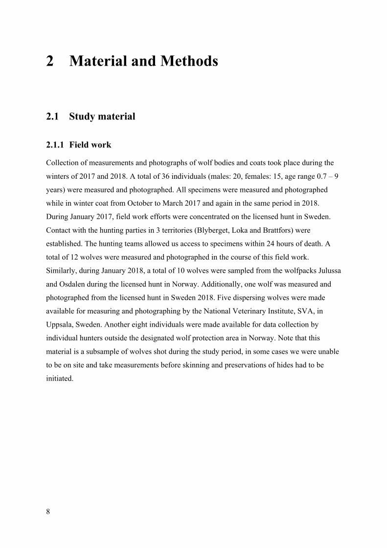
Collection of measurements and photographs of wolf bodies and coats took place during the

winters of 2017 and 2018. A total of 36 individuals (males: 20, females: 15, age range 0.7 – 9

years) were measured and photographed. All specimens were measured and photographed

while in winter coat from October to March 2017 and again in the same period in 2018.

During January 2017, field work efforts were concentrated on the licensed hunt in Sweden.

Contact with the hunting parties in 3 territories (Blyberget, Loka and Brattfors) were

established. The hunting teams allowed us access to specimens within 24 hours of death. A

total of 12 wolves were measured and photographed in the course of this field work.

Similarly, during January 2018, a total of 10 wolves were sampled from the wolfpacks Julussa

and Osdalen during the licensed hunt in Norway. Additionally, one wolf was measured and

photographed from the licensed hunt in Sweden 2018. Five dispersing wolves were made

available for measuring and photographing by the National Veterinary Institute, SVA, in

Uppsala, Sweden. Another eight individuals were made available for data collection by

individual hunters outside the designated wolf protection area in Norway. Note that this

material is a subsample of wolves shot during the study period, in some cases we were unable

to be on site and take measurements before skinning and preservations of hides had to be

initiated.

9

2.1.2 Museum collections

Wolf hides and skulls were made available for photography and external measurements by the

Natural History Museum in Oslo and the Swedish Museum of Natural History in Stockholm.

A total of 86 hides were photographed and 184 Scandinavian wolf skulls were measured.

Wolves reach adult size when they are about 12-14 months of age (Kreeger, 2010), and at an

age of about 24 months the major dimensions of skull is fully developed to maximum size

(Skeel & Carbyn, 1977; Nowak, 1979). Thus, since absolute age was not available for all

specimens, for this study wolves were primarily separated in to two life stages; adults and

juveniles. Individuals less than two years of age were classified as juveniles, and individuals

of two years of age and older were classified as adults. Notably, within these categories

individual variation in morphology does occur, and is often dependent on nutrient intake

(Kreeger, 2010). Information regarding specimens age at death was obtained from the

museums and Rovbase, a database and management tool that accumulates and verifies

information regarding carnivores in Norway and Sweden ("Rovbase, Miljødirektoratet and

Naturvårdsverket," 2018). Total numbers of specimens, sex, and life stage in all categories of

the study material is summarized in table 1. below. Of note, due to the scarcity of adult

females (n = 1) and relatively few juveniles (n = 4) available from the extinct population,

analysis of craniometrics data was restricted to adult males.

Table 1. Number of samples obtained from the extinct and extant Scandinavian population of grey wolf

Total Adult

Males

Adult

Females

Juvenile

Males

Juvenile

Females

Missing

information

on sex or

stage

Skulls, Extinct pop. 32 11 1 2 2 16

Skulls, Extant pop. 152 47 24 42 30 9

Hides, Extinct pop. 12 4 2 1 3 2

Hides, Extant pop. 72 21 10 20 17 4

Photographs, intact body 35 9 7 10 9 0

Measurements, intact body 35 9 7 10 9 0

10

2.2 Data collection

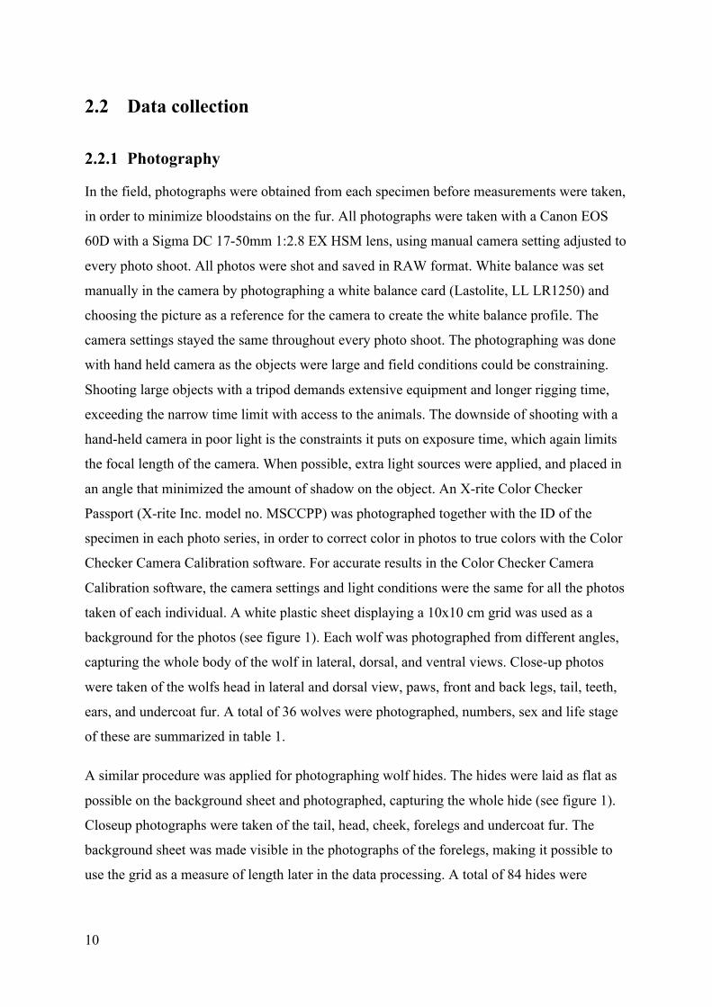
2.2.1 Photography

In the field, photographs were obtained from each specimen before measurements were taken,

in order to minimize bloodstains on the fur. All photographs were taken with a Canon EOS

60D with a Sigma DC 17-50mm 1:2.8 EX HSM lens, using manual camera setting adjusted to

every photo shoot. All photos were shot and saved in RAW format. White balance was set

manually in the camera by photographing a white balance card (Lastolite, LL LR1250) and

choosing the picture as a reference for the camera to create the white balance profile. The

camera settings stayed the same throughout every photo shoot. The photographing was done

with hand held camera as the objects were large and field conditions could be constraining.

Shooting large objects with a tripod demands extensive equipment and longer rigging time,

exceeding the narrow time limit with access to the animals. The downside of shooting with a

hand-held camera in poor light is the constraints it puts on exposure time, which again limits

the focal length of the camera. When possible, extra light sources were applied, and placed in

an angle that minimized the amount of shadow on the object. An X-rite Color Checker

Passport (X-rite Inc. model no. MSCCPP) was photographed together with the ID of the

specimen in each photo series, in order to correct color in photos to true colors with the Color

Checker Camera Calibration software. For accurate results in the Color Checker Camera

Calibration software, the camera settings and light conditions were the same for all the photos

taken of each individual. A white plastic sheet displaying a 10x10 cm grid was used as a

background for the photos (see figure 1). Each wolf was photographed from different angles,

capturing the whole body of the wolf in lateral, dorsal, and ventral views. Close-up photos

were taken of the wolfs head in lateral and dorsal view, paws, front and back legs, tail, teeth,

ears, and undercoat fur. A total of 36 wolves were photographed, numbers, sex and life stage

of these are summarized in table 1.

A similar procedure was applied for photographing wolf hides. The hides were laid as flat as

possible on the background sheet and photographed, capturing the whole hide (see figure 1).

Closeup photographs were taken of the tail, head, cheek, forelegs and undercoat fur. The

background sheet was made visible in the photographs of the forelegs, making it possible to

use the grid as a measure of length later in the data processing. A total of 84 hides were

11

photographed, 12 from the extinct population (year range 1830-1979) and 72 from the extant

(year range 1984-2016), for summary of sex and life stage see also table 1.

Figure 1. Photograph of a hide (Museum no. 20115040, NRM, Stockholm) with background sheet and color checker passport

12

2.2.2 Field morphometry

Morphological measurements were obtained from wolf bodies in the field. The collection of

measurements was carried out as fast as possible after the wolfs death, usually within 48

hours of death and before skinning of the hide. The specimens ID, age, sex, weight,

coordinates of capture and date of capture were noted. A total of 38 measurements were taken

on each specimen (figure 2, table 2), by using a measuring tape and vernier caliper.

Measurements were done to the nearest 0.1cm. Specimens were measured while lying down

on the side. When body length was measured, the wolfs neck was straightened out so the head

was linear with the shoulder. When limbs were measured, the limbs were held in a position

mimicking a wolf standing in an upright position. A total of 36 wolves were measured, see

table 1 for more detail. Measurements were only taken once due to the material only being

available for a restricted time period. The repeatability of these measurements should be

addressed in future studies.

Figure 2. Illustration of a grey wolf and definition of body measurements.

13

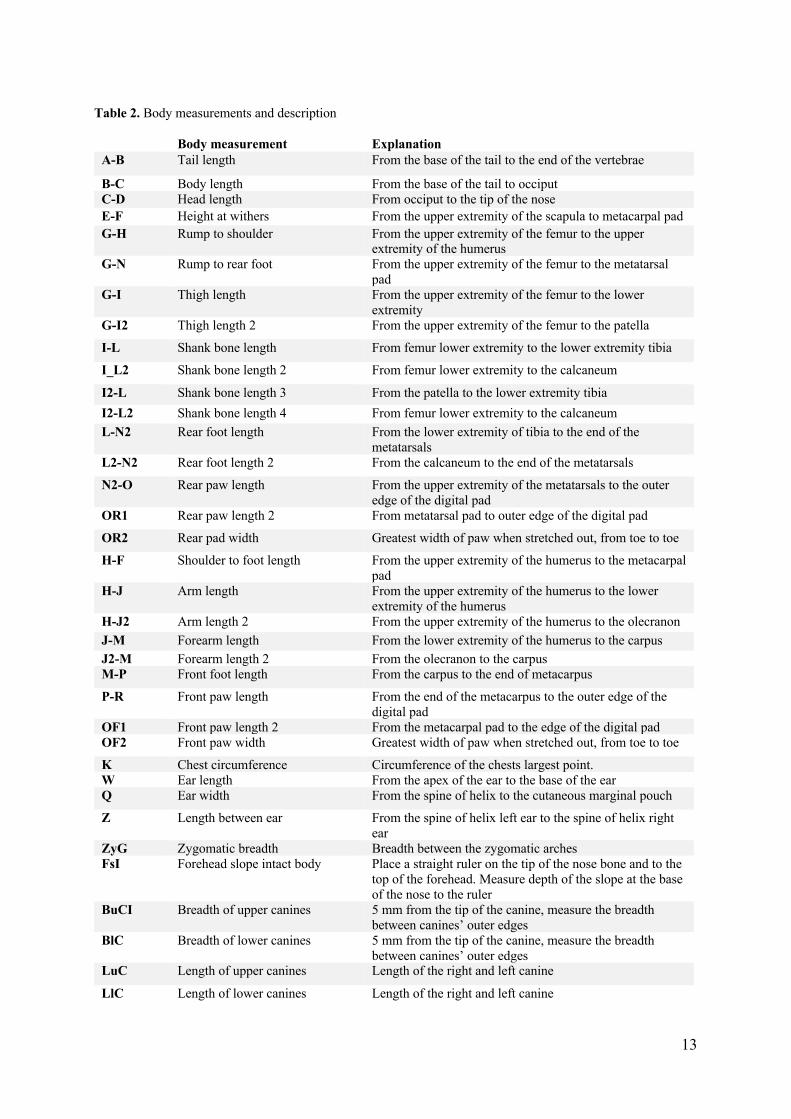
Table 2. Body measurements and description

Body measurement Explanation A-B Tail length From the base of the tail to the end of the vertebrae

B-C Body length From the base of the tail to occiput C-D Head length From occiput to the tip of the nose E-F Height at withers From the upper extremity of the scapula to metacarpal pad G-H Rump to shoulder From the upper extremity of the femur to the upper

extremity of the humerus G-N Rump to rear foot From the upper extremity of the femur to the metatarsal

pad G-I Thigh length From the upper extremity of the femur to the lower

extremity G-I2 Thigh length 2 From the upper extremity of the femur to the patella

I-L Shank bone length From femur lower extremity to the lower extremity tibia

I_L2 Shank bone length 2 From femur lower extremity to the calcaneum

I2-L Shank bone length 3 From the patella to the lower extremity tibia I2-L2 Shank bone length 4 From femur lower extremity to the calcaneum L-N2 Rear foot length From the lower extremity of tibia to the end of the

metatarsals L2-N2 Rear foot length 2 From the calcaneum to the end of the metatarsals

N2-O Rear paw length From the upper extremity of the metatarsals to the outer edge of the digital pad

OR1 Rear paw length 2 From metatarsal pad to outer edge of the digital pad

OR2 Rear pad width Greatest width of paw when stretched out, from toe to toe

H-F Shoulder to foot length From the upper extremity of the humerus to the metacarpal pad

H-J Arm length From the upper extremity of the humerus to the lower extremity of the humerus

H-J2 Arm length 2 From the upper extremity of the humerus to the olecranon J-M Forearm length From the lower extremity of the humerus to the carpus J2-M Forearm length 2 From the olecranon to the carpus M-P Front foot length From the carpus to the end of metacarpus

P-R Front paw length From the end of the metacarpus to the outer edge of the digital pad

OF1 Front paw length 2 From the metacarpal pad to the edge of the digital pad OF2 Front paw width Greatest width of paw when stretched out, from toe to toe

K Chest circumference Circumference of the chests largest point. W Ear length From the apex of the ear to the base of the ear Q Ear width From the spine of helix to the cutaneous marginal pouch

Z Length between ear From the spine of helix left ear to the spine of helix right ear

ZyG Zygomatic breadth Breadth between the zygomatic arches FsI Forehead slope intact body Place a straight ruler on the tip of the nose bone and to the

top of the forehead. Measure depth of the slope at the base of the nose to the ruler

BuCI Breadth of upper canines 5 mm from the tip of the canine, measure the breadth between canines’ outer edges

BlC Breadth of lower canines 5 mm from the tip of the canine, measure the breadth between canines’ outer edges

LuC Length of upper canines Length of the right and left canine

LlC Length of lower canines Length of the right and left canine

14

2.2.3 Skulls morphometry

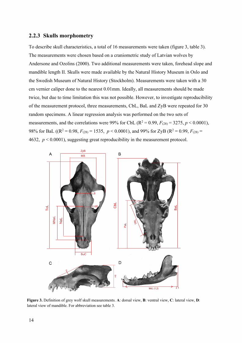
To describe skull characteristics, a total of 16 measurements were taken (figure 3, table 3).

The measurements were chosen based on a craniometric study of Latvian wolves by

Andersone and Ozolins (2000). Two additional measurements were taken, forehead slope and

mandible length II. Skulls were made available by the Natural History Museum in Oslo and

the Swedish Museum of Natural History (Stockholm). Measurements were taken with a 30

cm vernier caliper done to the nearest 0.01mm. Ideally, all measurements should be made

twice, but due to time limitation this was not possible. However, to investigate reproducibility

of the measurement protocol, three measurements, CbL, BaL and ZyB were repeated for 30

random specimens. A linear regression analysis was performed on the two sets of

measurements, and the correlations were 99% for CbL (R2 = 0.99, F(28) = 3275, p < 0.0001),

98% for BaL ((R2 = 0.98, F(28) = 1535, p < 0.0001), and 99% for ZyB (R2 = 0.99, F(28) =

4632, p < 0.0001), suggesting great reproducibility in the measurement protocol.

Figure 3. Definition of grey wolf skull measurements. A: dorsal view, B: ventral view, C: lateral view, D: lateral view of mandible. For abbreviation see table 3.

15

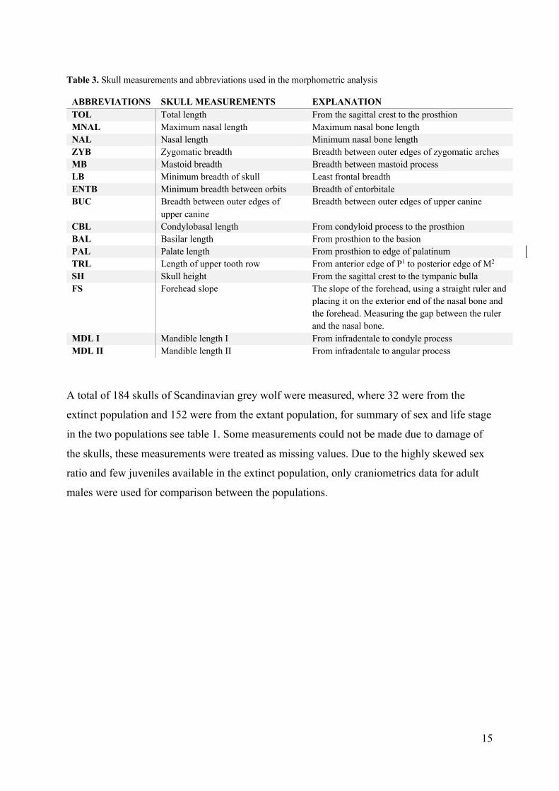
Table 3. Skull measurements and abbreviations used in the morphometric analysis

ABBREVIATIONS SKULL MEASUREMENTS EXPLANATION TOL Total length From the sagittal crest to the prosthion MNAL Maximum nasal length Maximum nasal bone length NAL Nasal length Minimum nasal bone length ZYB Zygomatic breadth Breadth between outer edges of zygomatic arches MB Mastoid breadth Breadth between mastoid process LB Minimum breadth of skull Least frontal breadth ENTB Minimum breadth between orbits Breadth of entorbitale BUC Breadth between outer edges of

upper canine Breadth between outer edges of upper canine

CBL Condylobasal length From condyloid process to the prosthion BAL Basilar length From prosthion to the basion PAL Palate length From prosthion to edge of palatinum TRL Length of upper tooth row From anterior edge of P1 to posterior edge of M2 SH Skull height From the sagittal crest to the tympanic bulla FS Forehead slope The slope of the forehead, using a straight ruler and

placing it on the exterior end of the nasal bone and the forehead. Measuring the gap between the ruler and the nasal bone.

MDL I Mandible length I From infradentale to condyle process MDL II Mandible length II From infradentale to angular process

A total of 184 skulls of Scandinavian grey wolf were measured, where 32 were from the

extinct population and 152 were from the extant population, for summary of sex and life stage

in the two populations see table 1. Some measurements could not be made due to damage of

the skulls, these measurements were treated as missing values. Due to the highly skewed sex

ratio and few juveniles available in the extinct population, only craniometrics data for adult

males were used for comparison between the populations.

16

2.3 Photograph processing

2.3.1 Foreleg mark

Photographs of wolf hide forelegs were initially processed in Adobe Photoshop CC (19.1.6.

Release). Standardizing an area of interest based on the individual size on hides is difficult

due to various skinning techniques and lack of bones as standardizing points. Instead, a 10x30

cm area of the foreleg and surrounding area, including all black markings, was extracted from

each image based on the background grid measurements and used as the area of interest for

further calculations. A brush tool in similar color as the fur was used in the area of interest to

remove holes, claws, background etc. that could affect the image analysis. Further processing

was performed in Fiji, an open-source software project for image analysis, building on the

ImageJ platform (Schindelin et al., 2012). Images were converted to 8-bit, before a threshold

filter was applied. Threshold filter paints out dark contrast in images and was manually

adjusted for each image to fit the black pigmented area in the fur, by using the original image

as a reference. The software was used to find the number of pixels in the marked area relative

to the total number of pixels in the image and was converted to cm2. The outline of the

marked area was manually verified against the original photograph. When possible, both legs

were processed for each animal and the mean of the two legs were used in the analysis. Two

observers, one blinded and one non-blinded did the image processing and analysis in Fiji. A

linear regression analysis was performed on the results from the two observers. The

correlation between the two observers was 92 % (n = 84, R2 = 0.92, F(82) = 907, p < 0.0001).

Mean data from both observers were used in further analysis.

The same method of photo processing and analysis was applied for animals photographed in

the field. Initial attempts to quantify hue and intensity of general coat coloration were aborted

due to time constraints.

17

2.4 Statistical analysis

Statistical analysis was performed in R using RStudio 1.1.453 (RStudio_Team, 2016) and

visualized with the R package ggplot2 (Wickham, 2016).

2.4.1 Craniometrics

I first performed an exploratory Principal component analysis (PCA) to determine which

variables contributed the most to variance within the data set. Principal component analysis is

a multivariate statistical technique which simplifies large data matrices with related variables.

This is done using orthogonal transformation to extract the dominant pattern and estimate

correlation structure of variables in the data matrix, creating a new set of variables called

principal components (PCs) (Wold et al., 1987; Abdi & Williams, 2010). The outcome of the

PCA can be visualized graphically by using the variables or individuals factor scores as

coordinates in the components space (Abdi & Williams, 2010).

Principal component analysis of craniometric measurements was performed using

FactoMineR (Lê et al., 2008) and visualized with factoextra (Kassambara & Mundt, 2017).

As PCAs require complete datasets an imputation was done using the missMDA package

(Josse & Husson, 2016) to estimate parameters for an incomplete dataset using a principal

component method (Josse & Husson, 2016). Only adult males were used in the PCA. Adult

females were excluded from the analysis due to low sample size of females. Due to greater

variation in juvenile skulls properties due to growth, combined with a low number of

juveniles in the extinct population, juveniles were also excluded from the analysis.

Consequently, only adult males were used in the PCA. The morphometric dataset used in the

PCA thus contained 16 measurements from 58 adult males, 11 extinct and 47 extant. Principal

component analysis requires linearity of the dataset, and deviation from linearity was not

detected for any of the PC’s or their most contributing (<5%) variables (Runs test, data not

shown). To test for population differences in PC values and in the greatest contributing

variable in differing PC’s, a non-parametric Mann-Whitney U-test was used due to the

difference in sample size.

18

2.4.2 Foreleg mark

Due to considerably unequal n in the two populations, data on foreleg melanin markings were

compared between the extinct and extant population by non-parametric Mann-Whitney U-

test. Effects of possibly confounding variables such as sex, season of capture, life stage and

somatic length and length of the foreleg (known for field specimens) were assessed by GLM.

Although these data met parametric criteria, this approach was not used to assess actual

population differences due to it’s possible sensitivity to unequal sample sizes (Keppel &

Wickens, 2004). GLM on field data revealed that life stage (adult vs juvenile) but not leg

length or length of the animal as such had a significant effect on melanised area. Life stage

did not vary systematically between the extinct and extant population, so it is assumed that

this possibly confounding variable did not affect the comparison between the populations

mentioned above.

Foreleg length from the field data was calculated by adding forearm length (J-M) with the

length of the front foot (M-P) and the front paw (P-R) (figure 2, table 2). A Shapiro-Wilk

normality test was applied to test for normality of data, and a two-sample t-test was conducted

to test for differences in foreleg length between juveniles (n = 21) and adult (n = 16) from the

field dataset.

19

3 Results

3.1 Skull morphometry in in the extinct and extant Scandinavian wolf population

In the principal component analysis, the four first principle components each explained more

than 5%, and together 85.2% of the total variation in the data set (Eigenvalues: PC1 = 9.87;

PC2 = 1.73; PC3 = 1.10; PC4 = 0.93), (figure 4). Principal components explaining less than

5% of the variance were excluded from further analysis.

Figure 4. Scree plot over percentage of explained variance for ten principal components. PC1, 2, 3 and 4 together explained 85.2% of the total variation.

20

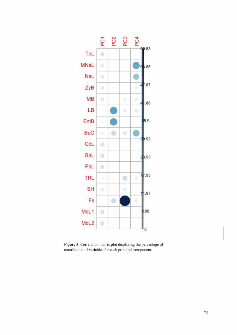
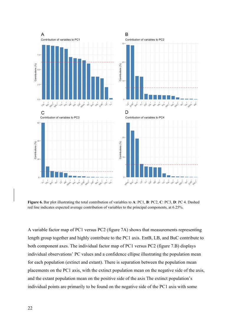
A correlation matrix plot (figure 5) illustrates the percentage each variable contributes to the

principal components, showing that a majority of the variables greatly contribute to PC1. For

PC1, ten variables are shown to range above the expected average contribution line at 6.25%

(figure 6.A). The six first variables stand out with the greatest contribution to PC1. These

variables, CbL, BaL, MdLII, MdLI, ToL and PaL (figure 3), are all measurements related to

skull length. The next variables contributing to PC1 which are not related to measurements of

length are MB and ZyB. These variables are measurements related to the width of the skull

(figure 3). The correlation matrix (figure 5) illustrates that PC2, PC3, and PC4 have fewer

variables that largely contribute to the components. Minimum width of skull (LB) and

minimum width between orbits (EntB) are measurements related to forehead width. These

two variables contributed most to PC2 (figure 6B), which explains 10.8% of the overall

variation. Forehead slope (Fs) is the greatest contributor of the variables in PC3 (figure 6.C),

which explains 6.9% of total variation. The variables with the greatest contribution to PC4,

which explained 5.8% of total variation, are MNaL and NaL, measurements of nasal length,

and BuC, which is the measurement of width between the upper canines (figure 6D).

21

Figure 5. Correlation matrix plot displaying the percentage of contribution of variables for each principal component.

22

A variable factor map of PC1 versus PC2 (figure 7A) shows that measurements representing

length group together and highly contribute to the PC1 axis. EntB, LB, and BuC contribute to

both component axes. The individual factor map of PC1 versus PC2 (figure 7.B) displays

individual observations’ PC values and a confidence ellipse illustrating the population mean

for each population (extinct and extant). There is separation between the population mean

placements on the PC1 axis, with the extinct population mean on the negative side of the axis,

and the extant population mean on the positive side of the axis The extinct population’s

individual points are primarily to be found on the negative side of the PC1 axis with some

Figure 6. Bar plot illustrating the total contribution of variables to A: PC1, B: PC2, C: PC3, D: PC 4. Dashed red line indicates expected average contribution of variables to the principal components, at 6.25%.

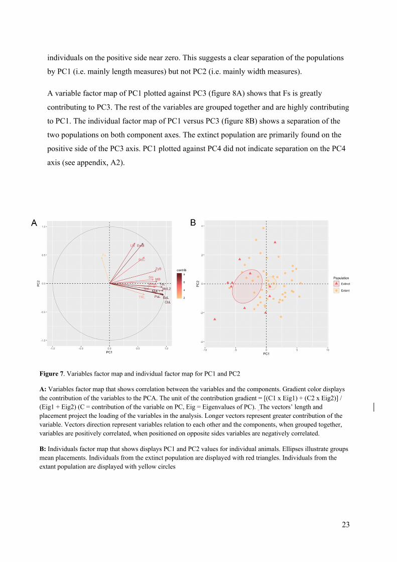
23

individuals on the positive side near zero. This suggests a clear separation of the populations

by PC1 (i.e. mainly length measures) but not PC2 (i.e. mainly width measures).

A variable factor map of PC1 plotted against PC3 (figure 8A) shows that Fs is greatly

contributing to PC3. The rest of the variables are grouped together and are highly contributing

to PC1. The individual factor map of PC1 versus PC3 (figure 8B) shows a separation of the

two populations on both component axes. The extinct population are primarily found on the

positive side of the PC3 axis. PC1 plotted against PC4 did not indicate separation on the PC4

axis (see appendix, A2).

Figure 7. Variables factor map and individual factor map for PC1 and PC2

A: Variables factor map that shows correlation between the variables and the components. Gradient color displays the contribution of the variables to the PCA. The unit of the contribution gradient = [(C1 x Eig1) + (C2 x Eig2)] / (Eig1 + Eig2) (C = contribution of the variable on PC, Eig = Eigenvalues of PC). The vectors’ length and placement project the loading of the variables in the analysis. Longer vectors represent greater contribution of the variable. Vectors direction represent variables relation to each other and the components, when grouped together, variables are positively correlated, when positioned on opposite sides variables are negatively correlated.

B: Individuals factor map that shows displays PC1 and PC2 values for individual animals. Ellipses illustrate groups mean placements. Individuals from the extinct population are displayed with red triangles. Individuals from the extant population are displayed with yellow circles

24

The individual PC scores were used to statistically test for significant differences between

populations for each principal component. Due to low sample size in the extinct population, a

non-parametric Mann-Whitney U-test was applied. There were significant differences

between the populations in PC1 (W = 410, p = 0.002) and PC3 (W = 118, p = 0.004), (Figure

9). There were no significant difference between the populations in PC2 (W = 284, p = 0.62)

or PC4 (W = 209, p = 0.33).

The variables with greatest contribution to PC1 and PC3 were also compared between the

populations using a Mann-Whitney U-test. Significant differences were found between the

two populations in Condylobasal length (CbL), (W = 357, p = 0.004), where the extant

population had higher mean value than the extinct population (figure 10A). In the case of

forehead slope (Fs), (W = 61.5, p = 0.006), the extinct population exhibit a greater mean slope

than the extant population (figure 10.B). This suggest that the extant population has longer

and flatter skulls than the extinct population.

Figure 8. Variables factor map and individual factor map for PC1 and PC3

A: Variables factor map that shows correlation between the variables and the components. Gradient color displays the contribution of the variables to the PCA. The unit of the contribution gradient = [(C1 x Eig1) + (C2 x Eig2)] / (Eig1 + Eig2) (C = contribution of the variable on PC, Eig = Eigenvalues of PC). The vectors’ length and placement project the loading of the variables in the analysis. Longer vectors represent greater contribution of the variable. Vectors direction represent variables relation to each other and the components, when grouped together, variables are positively correlated, when positioned on opposite sides variables are negatively correlated.

B: Individuals factor map that shows displays PC1 and PC3 values for individual animals. Ellipses illustrate groups mean placements. Individuals from the extinct population are displayed with red triangles. Individuals from the extant population are displayed with yellow circles

25

Figure 9. Boxplot comparing PC values between the populations. A: PC1, Mann-Whitney U: W = 410, p = 0.002, B: PC3, Mann-Whitney U: W = 118, p = 0.004

Figure 10. A: Condylobasal length (CbL) for the extinct and extant populations Mann-Whitney U: W = 357, p = 0.004 B: Measurement of forehead slope (Fs) for the two populations, Mann-Whitney U: W = 61.5, p = 0.006

26

Correlation between age and the measurements CbL and Fs was tested for each population

using linear regression analysis. There were no significant effect of age on CbL in either the

extinct or extant population (figure 11). Fs was not related to age in the extinct population

(figure 12A), but weakly so in the more numerous specimens from extant population (R2 =

0.12, p = 0.04, figure 12B). Correlation between age and the principal components were also

tested, but not found to be present (data not shown).

Figure 11. Linear regression between CbL and age. A: Extinct population, R2 = 0.04, p = 0.64. B: Extant population, R2 = 0.05, p = 0.18.

Figure 12. Linear regression between Fs and individual age. A: Extinct population, R2 = 0.001, p = 0.93. B: Extant population, R2 = 0.12, p = 0.04.

27

3.2 Foreleg mark size

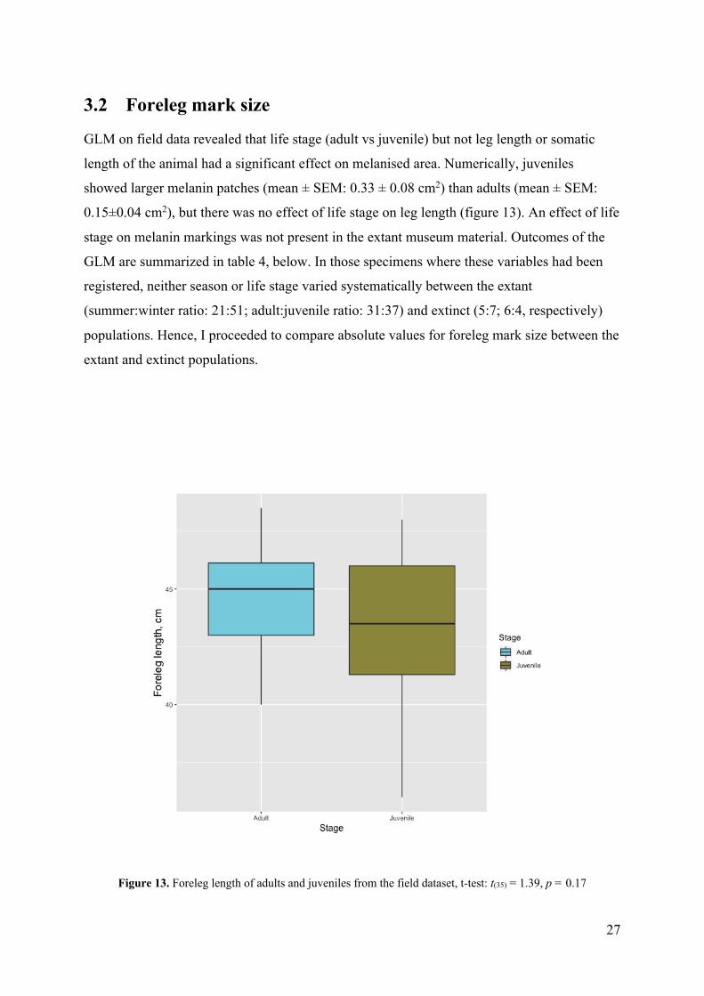
GLM on field data revealed that life stage (adult vs juvenile) but not leg length or somatic

length of the animal had a significant effect on melanised area. Numerically, juveniles

showed larger melanin patches (mean ± SEM: 0.33 ± 0.08 cm2) than adults (mean ± SEM:

0.15±0.04 cm2), but there was no effect of life stage on leg length (figure 13). An effect of life

stage on melanin markings was not present in the extant museum material. Outcomes of the

GLM are summarized in table 4, below. In those specimens where these variables had been

registered, neither season or life stage varied systematically between the extant

(summer:winter ratio: 21:51; adult:juvenile ratio: 31:37) and extinct (5:7; 6:4, respectively)

populations. Hence, I proceeded to compare absolute values for foreleg mark size between the

extant and extinct populations.

Figure 13. Foreleg length of adults and juveniles from the field dataset, t-test: t(35) = 1.39, p = 0.17

28

Table 4. GLM effect tests for possible confounding variables affecting foreleg mark size.

Field data DF Chi Square p

Sex 1 0.39 0.54

Life stage 1 4.78 0.03

Foreleg length 1 0.15 0.70

Somatic length 1 0.49 0.48

Museum specimens, DF Chi Square p

extant population

Sex 1 0.15 0.70

Life stage 1 0.43 0.50

Season 1 0.01 0.90

29

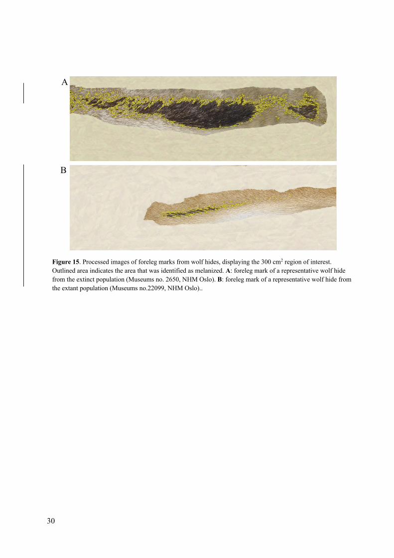
A non-parametric Mann-Whitney U-test was performed to investigate foreleg mark size

differences between the extinct (n = 12) and extant (n = 72) populations. A significant

difference in foreleg mark between the populations was found (W = 31, p < 0.001). As

illustrated in figure 14, the extinct population carried significantly larger foreleg marks than

the extant population (also, see representative examples in figure 15 and 16).

Figure 14. Boxplot of foreleg mark size in the extinct (n = 12) and extant (n = 72) population. The extinct population carried larger melanin marks than the extant population (W = 31, p < 0.001, Mann-Whitney U-test)

30

A

B

Figure 15. Processed images of foreleg marks from wolf hides, displaying the 300 cm2 region of interest. Outlined area indicates the area that was identified as melanized. A: foreleg mark of a representative wolf hide from the extinct population (Museums no. 2650, NHM Oslo). B: foreleg mark of a representative wolf hide from the extant population (Museums no.22099, NHM Oslo)..

31

A

B

Figure 166. Hides photographed at the Natural History Museum in Oslo, A: Foreleg of a wolf from the extinct population (Museum no. 2649, NHM Oslo). B: Foreleg of a wolf from the extant population (Museum no. 11204, NHM Oslo).

32

4 Discussion

4.1 Methodical considerations

A main aim of this study was to develop a method for obtaining standardized methods for

obtaining photographic documentation and morphological measurements to characterize

phenotypic traits in wolves. Before discussing the results of the study, I will recapitulate some

methodological considerations.

Firstly, obtaining reliable data from intact specimens in the field incurred a range of

challenges. The time specimens were available in the field varied from some hours to two

days, however most animals were only available for sampling a few hours between the

animal’s death and the planned skinning of the hide. Most often, hunters or contracted

taxidermists kindly postponed their work, sometimes to late evening or night, for us to reach

the site and perform the registrations. It must thus be considered a methodological weakness

that morphological measures could not be taken twice, to obtain an indication of repeatability.

When time again becomes available, I will however assess what measures can be checked

against the standard background used for both skins and intact animals.

Furthermore, equipment needed to be available at short notice and with rigging time as

efficient as possible. In Scandinavia, the hunt for wolves are usually carried out in the winter

months and daylight is consequentially limited. Applying extra light sources was required in

most of the photoshoots, as specimens usually became available for photographing and

measuring in the afternoon. To avoid creating hard shadows, two strong high-lumen lamps

were placed above head height. Ideally, applying more lamps would make rigging to avoid

shadows easier. However, this would mean a heavier load of equipment to bring in the field

and rigging time would be longer. In addition, some locations were lacking power outlets and

the car battery was then used as a power source, limiting available power. Arrangements were

however sufficient for lighting conditions to remain constant throughout each photoshoot,

thus shooting in natural light when light conditions are changing fast is not advisable.

However, if shooting under stable light conditions is not an option, camera settings should be

recalibrated when necessary and the color checker passport visible in every image. Taking

photographs before taking measurements proved to be important, as some specimens were

33

still bleeding to some extent and minimizing bloodstains was critical for the following image

analysis.

From museum collections, skull morphometrics were obtained from the extinct and extant

Scandinavian population, and a total of 16 measurements were taken. Repeatability of these

measurements was testable, and was carried out for three variables resulting in > 98%

correlation between repeats indicated by linear regression analysis. While also suffering from

highly unequal sample sizes in the museum material, the developed method for photo

capturing and image analysis appeared robust, with high repeatability between observers, and

capable of detecting between-population variation.

4.2 The natural history of the grey wolf in Scandinavia

Notably, interpretation of the current results requires some knowledge of the natural history of

the wolf populations in concern. Wolves were once widely distributed throughout the

Northern hemisphere occupying a wide range of habitats (Mech & Boitani, 2003). Early

human cultures with a hunter and warrior way of life admired wolves for their hunting

techniques, and some cultures strived to emulate the wolf´s way of hunting (Boitani, 1995).

Their view of the animal was often reflected in the religious beliefs of these cultures, were the

wolf was given godlike status (Boitani, 1995). The shift in attitude towards the wolf changed

when human cultures started keeping and protecting livestock (Fritts et al., 2003). As human

settlement spread, and the cultivating of land expanded, wolves and humans increasingly

came in conflict (Boitani, 1995; Fritts et al., 2003). This was the beginning of a radical human

persecution of wolves in Europe which became well organized in the Middle Ages (Boitani,

1995). Consequently, wolf populations decreased and became fragmented, some became

isolated and other became extinct (Ellegren et al., 1996). The Scandinavian wolf history

followed the same pattern as the rest of Europe. Hunting statistics from 1846 to 1977 shows

that hundreds of wolves were killed each year until wolf populations rapidly declined in the

mid nineteenth century (Bjerve, 1978; Vila et al., 2003). The grey wolf in Scandinavia

became legally protected in 1966 and 1973 in Sweden and Norway respectably, but the

population was then considered functionally extinct (Wabakken et al., 2001).

In 1983, wolves were again reproducing in Scandinavia, as a breeding pair of wolves was

discovered in Värmland (Wabakken et al., 2001). They reproduced the following years, and a

34

new wolf population was established on the Scandinavian peninsula. The population consisted

of under 10 individuals during the 1980s and genetic variability was lost due to inbreeding

(Ellegren et al., 1996). In 1991, a new male contributes to the population, and the population

started to grow exponentially (Vila et al., 2003). These three individuals still contribute with

over 95% of the variation in the present gene pool (Jansson et al., 2015). Around the same

time as wolves reappeared in Scandinavia, ungulate populations had undergone a rapid

increase in population size (Austrheim et al., 2008), resulting in an abundance of prey for the

new population (Olsson et al., 1997).

Today, the Scandinavian population is estimated to consist of around 400 individuals

(Wabakken et al., 2018). The geographical origin of the source population is assumed to be

the neighboring populations in Finland and/or Russia, with around 750 km to the closest

breeding packs (Seddon et al., 2006). The dispersal corridor between the two populations is

narrow, and few individuals make it to the Scandinavian population, and even fewer

reproduce (Vila et al., 2003; Seddon et al., 2006). In view of the above, it should be noted that

the morphological differences documented between the extinct and extant population must be

interpreted and discussed while keeping in mind that they could represent random founder

effects, geographical origin, direct environmental influences or even rapid adaption to the

current environment.

4.3 Results in brief

As mentioned, regarding craniometric measures from museum specimens, only adult males

were considered, with a final number of 11 representatives of the extinct population and 47

from the extant population. The results from the PCA showed that the first component

explained 61.7% of the total variance found, and the three following components explained

just over five percent each. The six variables that contributed most to PC1 are all various

measurements of skull length and the most contributing variable was Condylobasal length

(CbL). In PC2 the most contributing variables were measurements of skull width, for PC3 the

most contributing variable was forehead slope, and measurements representing nasal length

contributed most to PC4. The principal component analysis indicated a separation of the two

populations on PC1 and PC3, but not on PC2 and PC4. The individual factor scores from the

PC was indeed found to be significant between the populations on PC1 and PC3. A separate

Mann-Whitney U-test was also conducted on the variables that contributed most to PC1 and

35

PC3 between the populations. Condylobasal length was significantly longer in the extant

population than in the extinct population, indicating that the extant population has longer

skulls than the extant. Forehead slope was significantly greater in the extinct population than

the extant population, indicating a greater curve of the forehead in the extinct population.

Correlation between age and these two variables (CbL and Fs) was tested to investigate if

adult age had an impact on these skull measurements in each population. Variation in age was

not related to CbL, and could thus not explain the difference between the populations. Age

and forehead slope did not correlate in the extinct population, however, a weak but significant

relationship between age and forehead slope was detected in the extant population. Linear

regression between age and the four principal components was also tested, and no correlation

was indicated. Notwithstanding the considerable difference in sample size between the

populations, the possibility that age of the specimens contributed to Fs and hence PC3

variation should be considered as a possible explanation for this particular contrast between

extinct and extant wolves. Length of the skull, on the other hand, must be assumed to diverge

due to other biological factors (see discussion below).

Regarding foreleg melanin markings, the extinct population displayed distinctly larger marks

than the extant population. Notably, the size of these melanin patches was not related to

foreleg leg or length of the animal, indicating a functional difference in melanin synthesis

underlying pronounced vs weak melanisation. Possible mechanisms will be discussed below.

4.4 Skull morphology

The grey wolf has adapted to a range of different habitats, and consequently different

populations of wolves display different morphology in size, color and skull features (Milenvić

et al., 2010). The variation in morphology between populations is greatest along the north-

south directional axis (Nowak, 2003), and can be put in relation with the changes in

environmental variables on the same axis (Pilot et al., 2006). My results indicate that adult

male skull morphology differs between the extinct and extant Scandinavian wolf population.

The differences found was related to skull length and the depth of the skull curve between the

forehead and the nasal bone, and in short, the extant population exhibits a longer and flatter

skull than the extinct population.

36

Pinpointing the causal factors behind this observation cannot be achieved within the scope of

this thesis. I will however briefly discuss possible explanatory factors below. Environmental

factors is one such possible driver for variation skull morphology. Local adaptions to different

habitats could be the source to the variation in skull traits, and provided that the founding

individuals were representative of their population, the extant population may share these

traits with the source population. Intraspecific variation in morphology has been addressed by

a number of studies, with an emphasis on skull variation. Such variation can occur over

surprisingly narrow geographic and environmental ranges. For instance, Okarma and

Buchalczyk (1993) found a difference in cranimetric caracters between mountain and lowland

populations of wolves in Poland, where males from the mountain popuation had generally

larger skulls than the males from the lowland population. Milenković et. al. (2010) studied

morphometric variation in skulls between wolf populations in Serbia. They found that

Carpathian wolves were larger than Dinaric-Balkan wolves and the latter had a more elevated

snout and sagittal crest (Milenvić et al., 2010). Further, they present Bergmann´s rule (that

larger size is an adaption to colder environments) as a possible explanation for cranial size

differences. However, Bergmann´s rule is unlikely to explain the differences in skull traits

found in the Scandinavian populations, as the source population of the extant population is

likely to be found on comparable latitudes to todays core distribution area for wolves in

Scandinavia. Notably, my results only suggest differences between the two populations in

length of the skull and curve of the forehead, and not in overall skull size.

A vast range of environmental and/or genetic factors may have contributed to the observed

divergence. Nutrient stress, for instance, affects skull growth patterns in mammals,

particularly at the fetal stage (Pucciarelli et al., 1990; Gonzalez et al., 2014; O'Keefe et al.,

2014). In Scandinavia, wolves mainly prey on ungulates, which also suffered a population

decline concurrent with human expansion (Olsson et al., 1997; Austrheim et al., 2008).

During the same time period as wolves were killed in large numbers, moose (Alces alces), red

deer (Cervus elaphus) and roe deer (Capreolus capreolus) reached historically low population

numbers, due to competition with domestic livestock and hunting pressure (Austrheim et al.,

2008). Hence, the extinct wolf population in Scandinavia probably experienced a decrease in

available resources due to a population decline in ungulates which reached critical low

numbers around 1920. In contrast, the new established wolf population encountered an

expeditious increase in ungulates, above all moose. Nutrient stress may thus have had an

37

impact on the extinct population, as they probably suffered nutrient stress to some extent,

however, no conclusions can be drawn from the available data.

The difference found between the extinct and extant population in skull length and curve of

the forehead may reflect adaption to different hunting strategies or prey, either geographic or

over time. Machado et al. (2018) investigated the stability and evolution of morphological

integration of skull traits in Carnivora. They found a distinction between canids and other

carnivores in changes in facial traits, especially snout length. Canids showed a higher

flexibility and evolvability in facial trait involving snout and nasal length and the relative

length of the face displayed the greatest variance (Machado et al., 2018). Such flexibility and

evolvability in facial traits may have increased the canids capacity to respond to natural

selection (Machado et al., 2018). Canids mostly rely on their head and teeth for apprehending

prey, and the morphology of the jaw vary amongst canids based on diet (Slater et al., 2009)

and hunting strategies (Figueirido et al., 2011). In carnivores, bite force, which correlates with

gape angle, is a good indicator of feeding ecology (Figueirido et al., 2011). The length and

breadth of the snout in canids reflect biteforce and loading stress in the skull when biting

(Slater et al., 2009). Specifically, an elongated and narrow jaw is faster to close at the expense

of bite force, while a short and broad jaw allows animals to produce a larger bite force while

experiencing less stress on the skull (Slater et al., 2009). Wolves are hypercarnivore cursorial

animals that usually hunt in packs (Van Valkenburgh, 2007). In contrast, solitary felids that

take down large prey require a wide gape to constrain and suffocate prey, pack hunting

hypercarnivores are less dependent on delivering a single bite with large bite force as their

hunting behavior involves a joint effort of delivering repeated slashing bites to take down

prey (Christiansen & Wroe, 2007; Figueirido et al., 2011). Even so, bite force is also

important for pack hunting canids (Slater et al., 2009), and on the expense of a wide gape

angle they have increased their bite force by lengthening the moment arms for the temporalis

and masseter muscles in comparison to other large carnivores (Figueirido et al., 2011).

With this information in mind, the new established wolf population appeared in a habitat

abundant with moose and little intraspecific competition. If their skulls were under selection

pressure due to a shift in prey (from domestic livestock to moose), one might have expected

to see longer skulls in the extinct population and a shortening of the snout in the extant

population. However, this is not the case, and alternative explanations remain uncertain. A

theoretical possibility is that wolves may not benefit from a shorter and broader skull, as they

38

already possess a high bite force compared to other hypercarnivore canids (Damasceno et al.,

2013), Furthermore, a study conducted by Olsson et al. (1997) investigated the predation

pattern of the wolf population in Scandinavia from 1988-1992, when the population size was

around ten individuals or less. They found that wolves killed roe deer twice as often as moose,

despite that the moose density was around three times larger than of roe deer. The possibility

should also be considered that, despite the observed capacity for rapid evolution in canids, the

observed pattern in skull morphology does not reflect adaptation, but random founder effects.

After all, the contemporary population is considered to be solely the offspring of immigrants

from an undefined region in neighboring countries. In summary, further studies should

consider both founder effects, genetic drift, and inbreeding as possible mechanisms for the

observed variation in skull morphology.

4.5 Foreleg melanin patches

When various wolf populations have been described in literature, a dark mark or stripe

running down the front leg has been mentioned as a specific character (Pocock, 1935; Ognev,

1962; Pulliainen, 1965; Castelló, 2018). Here, I investigated the characteristic foreleg mark in

the extinct and extant wolf population in Scandinavia and found that the mark differed

significantly in size between the two populations. The extinct population had overall larger

markings on their legs, while the extant population usually had a small stripe or no markings

at all. Conceivably, a broader sampling range could have revealed an interesting interaction

between season and life stage, since a difference between juveniles and adults were only

present in the dataset obtained exclusively during the winter season (i.e. present day field

data).

The observed color variation incur a wide range of possible functional explanations. Firstly,

stripes or patches of black can serve as camouflage, and foreleg markings of some

mammalian species have been suggested to be disruptive coloration (Caro, 2009). Disruptive

coloration are sets of color marks that breaks up the outline appearance of an animal to

prevent detection of the animals shape and are often in a contrasting color to the rest of the

pelage (Caro, 2005; Stevens & Merilaita, 2011). Also, prominent black marks are found in

numerous species of diurnal artiodactyla living in open landscapes and are thought to act as

disruptive markings to break up the outline of the legs (Stoner et al., 2003; Caro, 2005, 2009).

However, this theory in artiodactyla is disputed (Stoner et al., 2003), and there is little

39

evidence of disruptive colorization in predators. Breaking up the outline on the front of the

body could indeed potentially disturb danger assessment by prey, say with regards to

adjudging distance and direction of travel of approaching predators. A function in disruptive

coloration is possible to reconcile with the observation that the extinct and extant populations

display different sizes of the foreleg mark, given that the original population may have

evolved in a different environment than current wolves (see discussion about geographical

origin below).

Caro (2009) suggested that marks on the frontal surface of the forelegs of mammals could

serve as communication signal, since many of these species live in large social groups. He

further emphasizes that little is known about the placement and function of such marks.

Colorization used in intraspecific communication may signal reproductive condition, health

and dominance (Caro, 2005, 2011). Melanin patches found on the front of animals can also be

signals of dominance (Järvi & Bakken, 1984; Caro, 2011). In this context, it is intriguing that

field data suggested that juveniles express more foreleg melanisation than adults. Wolves

display a highly complex and hierarchical social behavior (Packard, 2003), but it would seem

controversial to suggest that juveniles generally enjoyed higher social rank than adults.

Like with skull morphology, nutritional and environmental factors may influence the

development of melanin patches. A classic example is the male lion (Panthera leo) where

dark mane is associated with high testosterone, longer reproductive span, higher nutrition and

age (West & Packer, 2002; Caro, 2005). In particular, dark color of lions mane have been

associated with high nutrition intake, where darker maned males have higher food intake than

lighter maned males (West & Packer, 2002). It is not unlikely that the extinct and the extant

population had different accessibility to food due to the low density of ungulates in a longer

time period before 1960 followed by a rapid increase of moose around 1970s. The direction of

this effect should however be exactly the opposite of what is observed, namely a weaker

signal in the current population. If there is a linkage between melanin production in the

foreleg of wolves and high nutrition, one would expect more coloration among the extant

Scandinavian wolf population than the extinct, however, this is not the case in my results.

However, the evidence support of linkage between nutrition and melanin production in lions

have been questioned and the relationship between melanin production and high nutrition in

mammals are less clear (Hill & McGraw, 2003).

40

Melanin is also associated with stress, in that animals that are less resistant to stress and

disease show reduced melanin production compared to those that cope well with the current

environment (Ducrest et al., 2008; Khan et al., 2016). Conceivably, migrants could be under

stress during exposure to new environments, but it is hard to see how such an environmental

effect could explain why we still see less pronounced melanin patches in the present

populations (c.f. current field data). Contrasting geographical origin of the extinct and extant

wolf population is perhaps a more likely explanatory factor for the observed color variation.

An investigation of the distribution of foreleg mark in wolves in Finland, Russia and

Scandinavia (extinct population) was done by Pulliainen (1965). He divided individuals in

two groups, those with black mark and those without and found that both color morphs are

found in Finland and Russia but not in Scandinavia, where all the individuals had distinct

foreleg marks. Further, the most common morph was possessing a black mark on the foreleg,

while individuals without the mark were more abundant in eastern parts of Finland

(Pulliainen, 1965).

Pulliainen (1965) suggested that the reason for the different phenotypes in Finland could be

related to the concept of subspecies of wolves, i.e. mixed breeding between the so designated

tundra wolf (Canis lupus albus) and the Eurasian wolf (Canis lupus lupus). The term

subspecies is often used in the description of wolves from different geographical regions.

Some studies designate about 12 subspecies of grey wolf (Sillero-Zubiri et al., 2004), and the

color morphs vary between the different subspecies (Castelló, 2018). However, the term

subspecies may be problematic for long-dispersing species such as wolves, as subspecies may

interbreed and hybridize (Robert et al., 2003). The tundra wolfs coat color is described as

light grey with some ochre shade and white paws (Castelló, 2018). It is not described with a

black mark on the front of the foreleg to my knowledge. Their distribution range is the tundra

zone of northern Europe and Asia (Nowak, 2003; Castelló, 2018). North-east of Finland seem

to be a meeting point between the Eurasian subspecies distribution and the tundra wolf

distribution (Nowak, 2003; Castelló, 2018), but how much the distribution of the subspecies

overlap or if any overlap occur is not known for certain.

Potentially, the mark on the front leg of wolves may have adaptive value for animals living in

woodland or forest and serve as a type of camouflage, whereas the absence of such stripe may

be an adaption to tundra and an arctic environment. If interbreeding between two potential

subspecies did occur, and heritability follows a non-Mendelian pattern, it could yield a

41

phenotype intermediate between a non-marked and highly marked variant. Such individuals

could potentially be the founders of the new established wolf population in Scandinavia,

given that Finland or Russia is the suggested origin of the population. Of note, interbreeding

between subspecies is just a hypothesis and should be addressed in further studies. The

foreleg stripe size found in the extant Scandinavian population may also be accurately

representative of a still present source population, without any occurrence of interbreeding

between subspecies or populations being involved.

42

5 Conclusions

This study documents morphological differences between two wolf populations inhabiting the

same geographical area in two different time periods. Data was obtained on craniometric

measures and size of the melanin patch found on forelegs. Significant differences between the

extinct and extant Scandinavian wolf populations were observed in measures related to skull

length and forehead slope, with the current population exhibiting a longer skull with less

pronounced curvature between the forehead and nasal bone than the extinct population.

Possible explanations for different skull morphology in these two wolf populations could be

adaptation to different environments, differences in attainable nutrition, or genetic founder

effects followed by inbreeding and/or random genetic drift. Foreleg melanin patches were

significantly larger in the extinct compared to the extant population. In other species distinct

melanin patches indicate good condition, social dominance, and stress and disease resistance.

Alternatively, in wolves this trait may bring adaptive value to individuals inhabiting forests by

serving as disruptive coloration in this type of landscape, since wolves inhabiting tundra and

arctic open landscapes are reported to not exhibit this trait. The small foreleg mark size

observed in the extant population may be a trait shared with the source population, and the

possible function of this trait in wolves should be further investigated. Further studies are also

needed to address proximate and as well as ultimate causes of the observed differences in

skull morphology between the study populations.

43

6 References Abdi, H., & Williams, L. J. (2010). Principal component analysis. Wiley interdisciplinary

reviews: computational statistics, 2(4), 433-459. Andersen, L. W., Harms, V., Caniglia, R., Czarnomska, S. D., Fabbri, E., Jędrzejewska, B., . . .

Pertoldi, C. (2015). Long-distance dispersal of a wolf, Canis lupus, in northwestern Europe. Mammal Research, 60(2), 163-168.

Andersone, Z., & Ozolins, J. (2000). Craniometrical characteristics and dental anomalies in wolves Canis lupus from Latvia. Acta Theriologica, 45(4), 549-558.

Asahara, M. (2013). Unique inhibitory cascade pattern of molars in canids contributing to their potential to evolutionary plasticity of diet. Ecology and evolution, 3(2), 278-285.

Austrheim, G., Solberg, E. J., Mysterud, A., Daverdin, M., & Andersen, R. (2008). Hjortedyr og husdyr på beite i norsk utmark i perioden 1949–1999. Rapport zoologisk serie, 2, 2008.

Bjerve, P. J. (1978). Jaktstatistikk 1846-1977/ Hunting statistics 1846-1977. Norges offisielle statistikk, A 955.

Boitani, L. (1995). Ecological and cultural diversities in the evolution of wolf-human relationship. In L. N. Carbyn, S. H. Fritts, & D. R. Seip (Eds.), Ecology conservation of wolves in a changing world (pp. 3-11). Edmonton, Alberta, Canada: Canadian Circumpolar Intitute, University of Alberta.

Boitani, L. (2003). Wolf Conservation and Recovery. In L. D. Mech & L. Boitani (Eds.), Wolves: Behavior, Ecology, and Conservation (pp. 317-340). Chicago, Illinois: The University of Chicago Press.

Bolnick, D. I., & Fitzpatrick, B. M. (2007). Sympatric speciation: models and empirical evidence. Annual Review of Ecology, Evolution, and Systematics, 38, 459-487.

Breitenmoser, U. (1998). Large predators in the Alps: the fall and rise of man's competitors. Biological conservation, 83(3), 279-289.

Caro, T. (2005). The adaptive significance of coloration in mammals. AIBS Bulletin, 55(2), 125-136.

Caro, T. (2009). Contrasting coloration in terrestrial mammals. Philosophical Transactions of the Royal Society of London B: Biological Sciences, 364(1516), 537-548.

Caro, T. (2011). The functions of black-and-white coloration in mammals. In M. Stevens & S. Merilaita (Eds.), Animal Camouflage: Mechanisms and Function (pp. 298-329). Cambridge: Cambridge University Press.

Castelló, J. R. (2018). Canids of the World: Wolves, Wild Dogs, Foxes, Jackals, Coyotes, and Their Relatives: Princeton University Press.

Christiansen, P., & Wroe, S. (2007). Bite forces and evolutionary adaptations to feeding ecology in carnivores. Ecology, 88(2), 347-358.

Clotfelter, E. D., Ardia, D. R., & McGraw, K. J. (2007). Red fish, blue fish: trade-offs between pigmentation and immunity in Betta splendens. Behavioral Ecology, 18(6), 1139-1145.

Curtis, A. A., Orke, M., Tetradis, S., & van Valkenburgh, B. (2018). Diet-related differences in craniodental morphology between captive-reared and wild coyotes, Canis latrans (Carnivora: Canidae). Biological Journal of the Linnean Society, 123(3), 677-693.

Damasceno, E., Hingst-Zaher, E., & Astúa, D. (2013). Bite force and encephalization in the Canidae (Mammalia: Carnivora). Journal of Zoology, 290(4), 246-254.

44

Delibes, M. (1990). Status and conservation needs of the wolf (Canis lupus) in the Council of Europe member states (Vol. 47): Council of Europe.

Djan, M., Maletić, V., Trbojević, I., Popović, D., Veličković, N., Burazerović, J., & Ćirović, D. (2014). Genetic diversity and structuring of the grey wolf population from the Central Balkans based on mitochondrial DNA variation. Mammalian Biology-Zeitschrift für Säugetierkunde, 79(4), 277-282.

Drake, A. G., & Klingenberg, C. P. (2010). Large-scale diversification of skull shape in domestic dogs: disparity and modularity. The American Naturalist, 175(3), 289-301.

Driscoll, C. A., Macdonald, D. W., & O'Brien, S. J. (2009). From wild animals to domestic pets, an evolutionary view of domestication. Proceedings of the National Academy of Sciences, 106(Supplement 1), 9971-9978.

Ducrest, A.-L., Keller, L., & Roulin, A. (2008). Pleiotropy in the melanocortin system, coloration and behavioural syndromes. Trends in ecology evolution, 23(9), 502-510.

Ellegren, H., Savolainen, P., & Rosén, B. (1996). The genetical history of an isolated population of the endangered grey wolf Canis lupus: a study of nuclear and mitochondrial polymorphisms. Philosophical Transactions of the Royal Society of London B: Biological Sciences, 351(1348), 1661-1669.

Fabbri, E., Miquel, C., Lucchini, V., Santini, A., Caniglia, R., Duchamp, C., . . . Boitani, L. (2007). From the Apennines to the Alps: colonization genetics of the naturally expanding Italian wolf (Canis lupus) population. Molecular ecology, 16(8), 1661-1671.

Figueirido, B., MacLeod, N., Krieger, J., De Renzi, M., Pérez-Claros, J. A., & Palmqvist, P. (2011). Constraint and adaptation in the evolution of carnivoran skull shape. Paleobiology, 37(3), 490-518.

Fitzpatrick, B., Fordyce, J., & Gavrilets, S. (2009). Pattern, process and geographic modes of speciation. Journal of evolutionary biology, 22(11), 2342-2347.

Fondon, J. W., & Garner, H. R. (2004). Molecular origins of rapid and continuous morphological evolution. Proceedings of the National Academy of Sciences, 101(52).

Fritts, S. H., Stephenson, R. O., Hayes, R. D., & Boitani, L. (2003). Wolves and Humans. In L. D. Mech & L. Boitani (Eds.), Wolves: Behavior, Ecology, and Conservation (pp. 289-316). Chicago, Illinois: The University of Chicago Press.

Geffen, E., Anderson, M. J., & Wayne, R. K. (2004). Climate and habitat barriers to dispersal in the highly mobile grey wolf. Molecular ecology, 13(8), 2481-2490.

Gonzalez, P. N., Lotto, F. P., & Hallgrímsson, B. (2014). Canalization and developmental instability of the fetal skull in a mouse model of maternal nutritional stress. American Journal of Physical Anthropology, 154(4), 544-553.

Gray, S. M., & McKinnon, J. S. (2007). Linking color polymorphism maintenance and speciation. Trends in ecology evolution, 22(2), 71-79.

Haglund, B. (1973). The wolf in Fennoscandia. IUCN PUBLICATIONS NEW SERIES Supplementary Paper No 43, 5.

Hamilton, W. D., & Zuk, M. (1982). Heritable true fitness and bright birds: a role for parasites? Science, 218(4570), 384-387.

Hill, G. E., & McGraw, K. J. (2003). Melanin, nutrition, and the lion's mane. Science, 299(5607), 660-660.

Hoekstra, H. E. (2006). Genetics, development and evolution of adaptive pigmentation in vertebrates. Heredity, 97(3), 222.

45

Horth, L. (2003). Melanic body colour and aggressive mating behaviour are correlated traits in male mosquitofish (Gambusia holbrooki). Proceedings of the Royal Society of London B: Biological Sciences, 270(1519), 1033-1040.

Jansson, M., Amundin, M., & Laikre, L. (2015). Genetic contribution from a zoo population can increase genetic variation in the highly inbred wild Swedish wolf population. Conservation Genetics, 16(6), 1501-1505. doi:10.1007/s10592-015-0738-9

Josse, J., & Husson, F. (2016). missMDA: a package for handling missing values in multivariate data analysis. Journal of statistical software, 70(1), 1-31.

Järvi, T., & Bakken, M. (1984). The function of the variation in the breast stripe of the great tit (Parus major). Animal Behaviour, 32(2), 590-596.

Kardos, M., Åkesson, M., Fountain, T., Flagstad, Ø., Liberg, O., Olason, P., . . . Ellegren, H. (2018). Genomic consequences of intensive inbreeding in an isolated wolf population. Nature ecology evolution, 2(1), 124.

Kassambara, A., & Mundt, F. (2017). factoextra: Extract and Visualize the Results of Multivariate Data Analyses. R package version 1.0.5. Retrieved from https://CRAN.R-project.org/package=factoextra

Keppel, G., & Wickens, T. (2004). The Linear Model and Its Assumptions. In Design analysis: A researcher’s handbook (4 ed.). Upper Saddle River, NJ: Pearson Prentice-Hall.

Khan, U. W., Øverli, Ø., Hinkle, P. M., Pasha, F. A., Johansen, I. B., Berget, I., . . . Omholt, S. W. (2016). A novel role for pigment genes in the stress response in rainbow trout (Oncorhynchus mykiss). Scientific reports, 6, 28969.

Kirkpatrick, M., & Barton, N. (2006). Chromosome inversions, local adaptation and speciation. Genetics, 173(1), 419-434.

Kirkpatrick, M., Johnson, T., & Barton, N. (2002). General models of multilocus evolution. Genetics, 161(4), 1727-1750.

Kittilsen, S., Johansen, I. B., Braastad, B. O., & Øverli, Ø. (2012). Pigments, parasites and personalitiy: towards a unifying role for steroid hormones? PloS one, 7(4), e34281.

Kittilsen, S., Schjolden, J., Beitnes-Johansen, I., Shaw, J., Pottinger, T. G., Sørensen, C., . . . Øverli, Ø. (2009). Melanin-based skin spots reflect stress responsiveness in salmonid fish. Hormones behavior, 56(3), 292-298.

Koolhaas, J., Korte, S., De Boer, S., Van Der Vegt, B., Van Reenen, C., Hopster, H., . . . Blokhuis, H. (1999). Coping styles in animals: current status in behavior and stress-physiology. Neuroscience Biobehavioral Reviews, 23(7), 925-935.

Kreeger, T. J. (2010). The Internal Wolf; Physology, Patology, and Pharmacology. In L. D. Mech & L. Boitani (Eds.), Wolves: behavior, ecology, and conservation (pp. 192-217): University of Chicago Press.

Laidlaw, J., Gelfand, Y., Ng, K.-W., Garner, H. R., Ranganathan, R., Benson, G., & Fondon III, J. W. (2007). Elevated basal slippage mutation rates among the Canidae. Journal of Heredity, 98(5), 452-460.

Lê, S., Josse, J., & Husson, F. (2008). FactoMineR: an R package for multivariate analysis. Journal of statistical software, 25(1), 1-18.

Liberg, O., Andrén, H., Pedersen, H.-C., Sand, H., Sejberg, D., Wabakken, P., . . . Bensch, S. (2005). Severe inbreeding depression in a wild wolf Canis lupus population. Biology letters, 1(1), 17-20.

Machado, F. A., Zahn, T. M. G., & Marroig, G. (2018). Evolution of morphological integration in the skull of Carnivora (Mammalia): Changes in Canidae lead to increased evolutionary potential of facial traits. Evolution.

46

Majerus, M. E. (1998). Melanism. Evolution in action. McGraw, K. J., & Hill, G. E. (2000). Differential effects of endoparasitism on the expression of

carotenoid-and melanin-based ornamental coloration. Proceedings of the Royal Society of London B: Biological Sciences, 267(1452), 1525-1531.

McKinnon, J. S., & Pierotti, M. E. (2010). Colour polymorphism and correlated characters: genetic mechanisms and evolution. Molecular ecology, 19(23), 5101-5125.

Mech, L. D. (1995). The challenge and opportunity of recovering wolf populations. Conservation biology, 9(2), 270-278.

Mech, L. D., & Boitani, L. (2003). Wolves: behavior, ecology, and conservation: University of Chicago Press.

Milenvić, M., Šipetić, V. J., Blagojević, J., Tatović, S., & Vujošević, M. (2010). Skull variation in Dinaric-Balkan and Carpathian gray wolf populations revealed by geometric morphometric approaches. Journal of Mammalogy, 91(2), 376-386.

Musiani, M., Leonard, J. A., Cluff, H. D., Gates, C. C., Mariani, S., Paquet, P. C., . . . Wayne, R. K. (2007). Differentiation of tundra/taiga and boreal coniferous forest wolves: genetics, coat colour and association with migratory caribou. Molecular ecology, 16(19), 4149-4170.

Nowak, R. M. (1979). North American Quaternary Canis. University of Kansas, Museum of Natural History. (Monogr. No. 6)

Nowak, R. M. (2003). Wolf evolution and taxonomy. In L. D. Mech & L. Boitani (Eds.), Wolves: Behavior, Ecology, and Conservation (pp. 239-258). Chicago, Illinois: The University of Chicago Press.

O'Keefe, F. R., Binder, W. J., Frost, S. R., Sadlier, R. W., & Van Valkenburgh, B. (2014). Cranial morphometrics of the dire wolf, Canis dirus, at Rancho La Brea: temporal variability and its links to nutrient stress and climate. Palaeontologia Electronica.

O'Keefe, F. R., Meachen, J., Fet, E. V., & Brannick, A. (2013). Ecological determinants of clinal morphological variation in the cranium of the North American gray wolf. Journal of Mammalogy, 94(6), 1223-1236.

Ognev, S. I. (1962). Mammals of Eastern Europe and Northern Asia. (Vol. II Carnivora). Smithsonian Institution and the National Science Foundation Washington DC by the Israel Program for Scientific Translations 1962

Olsson, O., Wirtberg, J., Andersson, M., & Wirtberg, I. (1997). Wolf Canis lupus predation on moose Alces alces and roe deer Capreolus capreolus in south-central Scandinavia. Wildlife biology, 3(1), 13-25.

Packard, J. M. (2003). Wolf Behavior: Reproductive, Social, and Intelligent. In L. D. Mech & L. Boitani (Eds.), Wolves: Behavior, Ecology, and Conservation. Chicago, Illinois: The University of Chicago Press.

Pilot, M., Greco, C., Jędrzejewska, B., Randi, E., Jędrzejewski, W., Sidorovich, V., . . . Wayne, R. (2014). Genome-wide signatures of population bottlenecks and diversifying selection in European wolves. Heredity, 112(4), 428.

Pilot, M., Jedrzejewski, W., Branicki, W., Sidorovich, V. E., Jedrzejewska, B., Stachura, K., & Funk, S. M. (2006). Ecological factors influence population genetic structure of European grey wolves. Molecular ecology, 15(14), 4533-4553.

Pimlott, D. H. (1973). The wolf in Europe in 1973. IUCN PUBLICATIONS NEW SERIES Supplementary Paper No 43, 5.

Pocock, R. I. (1935). The races of Canis lupus. Proceedings of the Zoological Society of London, 105(3), 647-686. Oxford, UK: Blackwell Publishing Ltd.

47

Pucciarelli, H. M., Dressino, V., & Niveiro, M. H. (1990). Changes in skull components of the squirrel monkey evoked by growth and nutrition: an experimental study. American Journal of Physical Anthropology, 81(4), 535-543.

Pulliainen, E. (1965). Studies on the wolf (Canis lupus L.) in Finland. Paper presented at the Annales Zoologici Fennici.

Radinsky, L. (1973). Evolution of the Canid Brain; pp. 169–185. Brain, Behavior and Evolution, 7(3), 169-185.

Razeto-Barry, P., Díaz, J., Cotoras, D., & Vásquez, R. A. (2011). Molecular evolution, mutation size and gene pleiotropy: a geometric reexamination. Genetics, 187(3), 877-885.

Robert, K., Wayne, & Vilà, C. (2003). Molecular Genetic Studies of Wolves. In L. D. Mech & L. Boitani (Eds.), Wolves: Behavior, Ecology, and Conservation (pp. 218-238). Chicago, Illinois: The University of Chicago Press.

Roulin, A. (2004). The evolution, maintenance and adaptive function of genetic colour polymorphism in birds. Biological Reviews, 79(4), 815-848.

Roulin, A., Almasi, B., Rossi-Pedruzzi, A., Ducrest, A.-L., Wakamatsu, K., Miksik, I., . . . Jenni, L. (2008). Corticosterone mediates the condition-dependent component of melanin-based coloration. Animal Behaviour, 75(4), 1351-1358.

Rovbase, Miljødirektoratet and Naturvårdsverket. (2018, 23.11.2018). Version 3.0.860. Retrieved from www.rovbase.no

RStudio_Team. (2016). RStudio: Integrated Development Environment for R. RStudio, Inc. (Version 1.1.453). Boston, MA. Retrieved from http://www.rstudio.com/

Räikkönen, J., Bignert, A., Mortensen, P., & Fernholm, B. (2006). Congenital defects in a highly inbred wild wolf population (Canis lupus). Mammalian Biology-Zeitschrift für Säugetierkunde, 71(2), 65-73.

Schindelin, J., Arganda-Carreras, I., Frise, E., Kaynig, V., Longair, M., Pietzsch, T., . . . Schmid, B. (2012). Fiji: an open-source platform for biological-image analysis. Nature methods, 9(7), 676.

Schoenebeck, J. J., & Ostrander, E. A. (2013). The genetics of canine skull shape variation. Genetics, 193(2), 317-325.

Seddon, J., Sundqvist, A.-K., Björnerfeldt, S., & Ellegren, H. (2006). Genetic identification of immigrants to the Scandinavian wolf population. Conservation Genetics, 7(2), 225-230.

Sherratt, T. N., & Beatty, C. D. (2003). The evolution of warning signals as reliable indicators of prey defense. The American Naturalist, 162(4), 377-389.

Sillero-Zubiri, C., Hoffmann, M., & Macdonald, D. W. (2004). Canids: foxes, wolves, jackals, and dogs: status survey and conservation action plan: IUCN Gland, Switzerland.

Sinervo, B., & Svensson, E. (2002). Correlational selection and the evolution of genomic architecture. Heredity, 89(5), 329.

Skeel, M. A., & Carbyn, L. N. (1977). The morphological relationship of gray wolves (Canis lupus) in national parks of central Canada. Canadian Journal of zoology, 55(4), 737-747.

Slater, G., Dumont, E., & Van Valkenburgh, B. (2009). Implications of predatory specialization for cranial form and function in canids. Journal of Zoology, 278(3), 181-188.

Stevens, M., & Merilaita, S. (2011). Animal camouflage. In M. Stevens & S. Merilaita (Eds.), Animal Camouflage: Mechanisms and Function (pp. 1-16). Cambridge: Cambridge University Press.

48

Stoner, C., Caro, T., & Graham, C. (2003). Ecological and behavioral correlates of coloration in artiodactyls: systematic analyses of conventional hypotheses. Behavioral Ecology, 14(6), 823-840.

Van Valkenburgh, B. (2007). Déjà vu: the evolution of feeding morphologies in the Carnivora. Integrative Comparative Biology, 47(1), 147-163.

Vila, C., Sundqvist, A. K., Flagstad, Ø., Seddon, J., Kojola, I., Casulli, A., . . . Ellegren, H. (2003). Rescue of a severely bottlenecked wolf (Canis lupus) population by a single immigrant. Proceedings of the Royal Society of London B: Biological Sciences, 270(1510), 91-97.

Vinkler, M., & Albrecht, T. (2010). Carotenoid maintenance handicap and the physiology of carotenoid-based signalisation of health. Naturwissenschaften, 97(1), 19-28.

von Schantz, T., Bensch, S., Grahn, M., Hasselquist, D., & Wittzell, H. (1999). Good genes, oxidative stress and condition–dependent sexual signals. Proceedings of the Royal Society of London B: Biological Sciences, 266(1414), 1-12.

Wabakken, P., Sand, H., Liberg, O., & Bjärvall, A. (2001). The recovery, distribution, and population dynamics of wolves on the Scandinavian peninsula, 1978-1998. Canadian Journal of zoology, 79(4), 710-725.

Wabakken, P., Svensson, L., Maartmann, E., Åkesson, M., & Flagstad, Ø. (2018). Bestandsovervåking av ulv vinteren 2017-2018.

Wayne, R. K. (1986). Cranial morphology of domestic and wild canids: the influence of development on morphological change. Evolution, 40(2), 243-261.

West, P. M., & Packer, C. (2002). Sexual selection, temperature, and the lion's mane. Science, 297(5585), 1339-1343.

Wheeldon, T. J., & Patterson, B. R. (2012). Genetic and morphological differentiation of wolves (Canis lupus) and coyotes (Canis latrans) in northeastern Ontario. Canadian Journal of zoology, 90(10), 1221-1230.

Wickham, H. (2016). ggplot2: elegant graphics for data analysis: Springer. Wiig, Ø., & Bachmann, L. (2014). Fluctuating asymmetry and inbreeding in Scandinavian gray

wolves (Canis lupus). Acta Theriologica, 59(3), 399-405. Wold, S., Esbensen, K., & Geladi, P. (1987). Principal component analysis. Chemometrics

intelligent laboratory systems, 2(1-3), 37-52. Øverli, Ø., Sørensen, C., Pulman, K. G., Pottinger, T. G., Korzan, W., Summers, C. H., &

Nilsson, G. E. (2007). Evolutionary background for stress-coping styles: relationships between physiological, behavioral, and cognitive traits in non-mammalian vertebrates. Neuroscience Biobehavioral Reviews, 31(3), 396-412.

Åkesson, M., Liberg, O., Sand, H., Wabakken, P., Bensch, S., & Flagstad, Ø. (2016). Genetic rescue in a severely inbred wolf population. Molecular ecology, 25(19), 4745-4756.

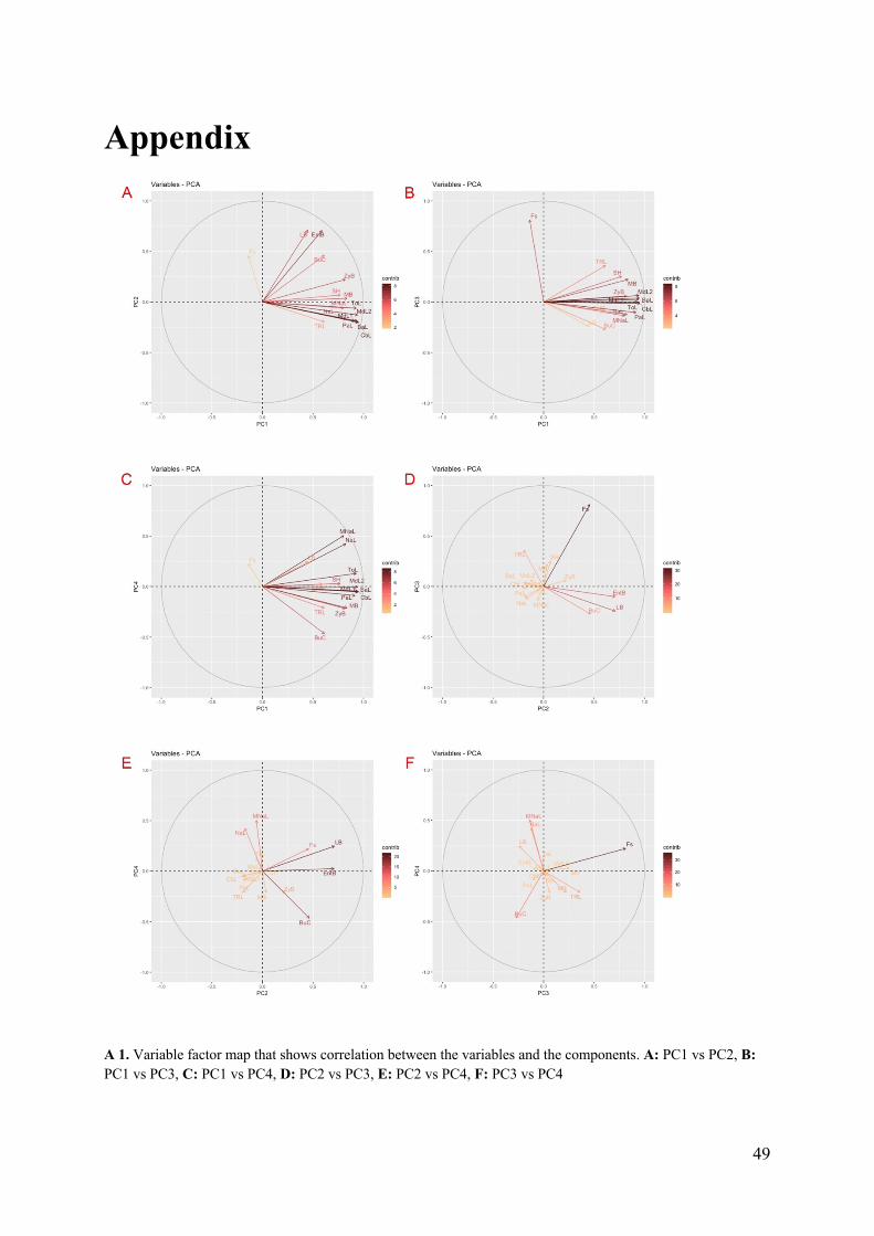
49

Appendix

A 1. Variable factor map that shows correlation between the variables and the components. A: PC1 vs PC2, B: PC1 vs PC3, C: PC1 vs PC4, D: PC2 vs PC3, E: PC2 vs PC4, F: PC3 vs PC4

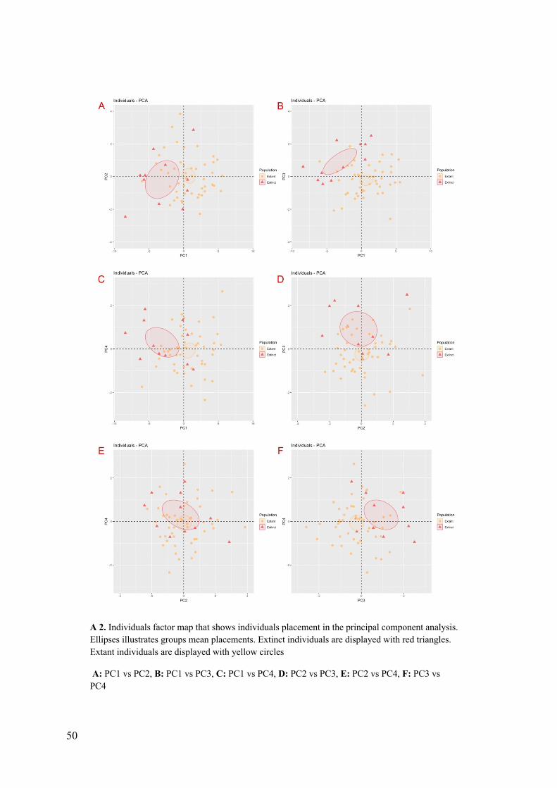
50

A 2. Individuals factor map that shows individuals placement in the principal component analysis. Ellipses illustrates groups mean placements. Extinct individuals are displayed with red triangles. Extant individuals are displayed with yellow circles

A: PC1 vs PC2, B: PC1 vs PC3, C: PC1 vs PC4, D: PC2 vs PC3, E: PC2 vs PC4, F: PC3 vs PC4

51