petri nets for modelling and analysing trophic networksceur-ws.org/vol-1373/paper2.pdf · petri...

Petri nets for modelling and analysingtrophic networks

Paolo Baldan1, Martina Bocci2, Daniele Brigolin2, Nicoletta Cocco2, andMarta Simeoni2

1 Dipartimento di Matematica, Universita di Padova, [email protected]

2 Dipartimento di Scienze Ambientali, Informatica e Statistica,Universita Ca’ Foscari di Venezia, Italy

{martina.bocci,brigo,cocco,simeoni}@unive.it

Abstract. We consider trophic networks, a kind of networks used inecology to represent feeding interactions (what-eats-what) in an ecosys-tem. We observe that trophic networks can be naturally modelled asPetri nets and this suggests the possibility of exploiting Petri nets forthe analysis and simulation of trophic networks. Some preliminary stepsin this directions and some ideas for future development are presented.

1 Introduction

Ecosystems are very complex systems constituted by biotic communities (popu-lations of different species), abiotic components of the environment (like air, wa-ter, soil) and interactions among these (living and non-living) elements. A branchof ecology deals with the study of feeding relationships within ecosystems andrepresents them as networks of interacting compartments called trophic networksor food webs. Due to the common limited availability of experimental informa-tion, a static approach (the mass balance steady state approach) to the study ofsuch networks has been developed as alternative to the dynamic description.

Complex networks of interacting entities are widely studied in computer sci-ence: computer networks, agent systems, and, in general, all concurrent anddistributed systems fall into this category. Uncountably many formalisms andpractical tools have been developed for the representation and analysis of inter-acting systems. This suggests the possibility of reusing models and techniquesfrom computer science for the study of trophic networks.

This idea is pursued in [17], where the authors advocate the use of processcalculi for ecological modelling. Their claim is that the compositionality prop-erties of process calculi can be fruitfully exploited for a modular representationof complex ecosystems. Moreover, process calculi provide an individual basedmodelling and stochastic extensions.

In this paper we explore the use of another widely used model of concur-rency, namely Petri nets [19, 11]. Petri nets permit individual based modelling,they explicitly represent parallelism and dependencies among entities, they offer

M Heiner, AK Wagler (Eds.): BioPPN 2015, a satellite event of PETRI NETS 2015, CEUR Workshop Proceedings Vol. 1373, 2015.

22 P Baldan et al.

stochastic and continuous extensions and, as a major advantage, they enablea qualitative analysis of systems when dynamic information are not available.Many tools for systems visualisation, analysis and simulation are also available(see The Petri net World site [21]). In this paper we consider the representationand analysis techniques generally adopted for trophic networks and discuss thepros and cons of the application of Petri nets to this field.

The structure of the paper is as follows. In Section 2 trophic networks areintroduced with a small case study related to the Venice lagoon. In Section 3 themain concepts in Petri nets used to model trophic networks are briefly recalled. InSection 4 we propose a simple application of Petri nets to the representation andanalysis of trophic networks when dynamic information are not available. Thisis exemplified in the case study. Some conclusions and suggestions for furtherwork are given in Section 5.

2 Tropic Networks

An ecosystem is a community of living organisms, such as plants, animals andmicrobes, in conjunction with the nonliving components of their environment,such as air, water and bioavailable organic matter (detritus), which interact asa system. A trophic network (or food web) is a representation of feeding inter-actions in an ecosystem, where the components are connected by binary links(what-eats-what). Food webs permit to represent and analyse the trophic struc-ture and functioning of an ecosystem. This knowledge can be used to identifykey species and to detect anthropogenic impacts, such as the effects of pollution,of physical disturbance, of resources exploitation, etc. Real trophic networks arevery complex, hence models provide partial and abstract representations where,for instance, similar species are aggregated into groups with similar feeding be-haviour. Model representation of a trophic network generally focuses on thefluxes of energy or biomass between nodes. Such fluxes are directional and gener-ally encompass some very relevant organism-level processes, such as production,consumption, assimilation, predation, non-predatory mortality and respiration.An ecosystem is generally an open system, i.e. there are flows of material orenergy between the system and the rest of the world. For this reason, when rep-resenting and analysing trophic networks, generally also the input and outputflows are taken into account. Inputs can be primary production, immigration orincoming of detrital matter into the system, while outputs can be emigration,harvesting by humans and exit of detrital matter from the system. Some energymay be dissipated into heat (respiration) or some material may be degraded intoits lowest energy form (detritus).

Knowledge on the species present in the studied ecosystem and on their feed-ing behaviour is a needed prerequisite for representing the trophic network. Firstof all it is necessary to single out the n living and non-living compartments to berepresented. A compartment can represent a population of a given species or ofsome aggregation of species with comparable feeding habits. For each compart-ment it is necessary to determine which other taxa are included in its diet, thus

Proc. BioPPN 2015, a satellite event of PETRI NETS 2015

Petri nets for trophic networks 23

Nocost. Flux1 CO2→PHP2 input→DET3 PHP→MIZ4 PHP→MEZ5 PHP→DET6 PHP→TAP7 DET→BPL8 BPL→CO2

9 BPL→MEZ10 BPL→MIZ11 BPL→TAP12 MIZ→MIZ13 MIZ→DET14 MIZ→CO2

15 MIZ→MEZ16 MIZ→TAP17 MEZ→MEZ18 MEZ→DET19 MEZ→CO2

20 TAP→DET21 TAP→CO2

22 TAP→Harvesting23 DET→TAP24 DET→Export

Fig. 1. A trophic network TV of the Venice Lagoon [4] (left) and its fluxes (right).

specifying the interactions among species or groups of species. These informationdetermine the network topology, which already provides some relevant insightson the features of the ecosystem. It is normally represented as a directed graphwhere each node represents a compartment and each arc denotes an interactionbetween the source and target nodes. More precisely, an arc from node A to nodeB represents a flow of energy or biomass from A to B. A common conventionis to depict dissipation for some node with an arc outgoing from the node andending in the ground symbol of electrical circuits [20]. A quantity may be asso-ciated with each arc, representing the magnitude of biomass or energy flow orthe relative occurrence of such a flow. The resulting graph is a directed weightedgraph.

The graph of a simple planktonic trophic network of the Venice Lagoon,taken from [4], is shown in Figure 1 (left). Numbers on arrows indicate thefluxes, which are listed in Figure 1 (right). The compartments considered arephytoplankton (PHP), bacterioplankton (BPL), microzooplankton (MIZ), meso-zooplankton (MEZ), R. philippinarum (TAP) and organic detritus (DET). Thenetwork provides a representation of the food items digested and assimilated byR. philippinarum (a marine bivalve mollusk), namely, green algae, cyanobacte-ria, diatoms, bacterioplankton, microzooplankton, and dead, dissolved, and/orparticulate organic matter.

This trophic network has some peculiarities:

– dissipation (respiration) of PHP is not considered because the flow from CO2

to PHP models the net photosynthetic production, known from experimentaldata, i.e. the CO2 needed for respiration has been already subtracted;


24 P Baldan et al.

– flow from BPL to DET (mortality of BPL) is not considered because it isknown to be negligible by experimental data;

– flows from TAP, MEZ and MIZ to DET include both natural mortality andproduction of faeces;

– flow from PHP to DET indicates only mortality, because PHP does notproduce faeces;

– in the case of MIZ and MEZ cannibalism is represented by arrows exitingand entering in the same compartment (flows 12 and 17).

From the topology of the graph, or the corresponding adjacency matrix, some in-formation about system behaviour can be derived. Clearly the adjacency matrixdoes not represent the information on weights of the interactions. For this reasonvarious other matrices have been defined and used for analysis purposes, such asthe matrix of dietary coefficients, the Leontief structure matrix, the total depen-dency matrix and many others which express different views of the network inrelation to structural and quantitative dependencies among compartments [28].The main advantage of a matrix representation of a trophic network is that lin-ear algebra techniques can be applied and in fact matrix methods are the mostused for static analysis of trophic networks (e.g. I-O modelling techniques foreconomics modified for ecosystems [28]).

To move from purely topological analysis of a trophic network to quantitativeanalysis, ecologists need quantitative data. Estimation of biomass and knowledgeof several rates (e.g. production rate, consumption rate, respiration rate, etc.)are needed to quantify flows among compartments, together with quantitativeknowledge about diet composition of each living compartment. Some informa-tion on primary production, specific consumption rates and diet compositionscan be gained from field and laboratory studies but it is unfeasible to deter-mine the magnitudes of all flows in the system directly. It becomes necessary,therefore, to estimate the magnitudes of some of them by indirect means. Ahelpful approach for estimating unknown flows consists in assuming the bal-ance of inputs and outputs for each compartment. If a sufficiently long timeperiod is considered, mass balance in each node of the network is a reasonableassumption because of the conservation of mass principle. Under the mass bal-ance assumption, the system is represented as a steady state snapshot of energyflows, averaged over time. Different techniques are used for the trophic networkreconstruction, that is to infer unspecified flows by solving the balance equa-tions and satisfying the constraints among the flows in the system. The problemis generally underdetermined and an infinite number of solutions comply withthe data set and the mass balance assumption. One technique is the InverseModel (IM), which has been firstly applied to trophic network in [31] and it hasbecome quite common among ecologists. IM combines mass balance equations,data equations and constraints on the flows expressed as inequalities. It finds aunique solution based on some optimisation criteria, for example by minimisingthe sum of squared flows, which corresponds to the most parsimonious solution.The package LIM implements linear inverse models in R [29]. Another freelyavailable popular automated balancing routine that supports representation of



trophic networks, estimation of unknown flows and ecological network analysisis Ecopath [6] and its evolutions Ecopath-Ecosym-Ecospace [7, 8].

Several analyses on ecological networks have been defined in the last decades.Some of them are based only on the topology of the model, for instance deter-mining food chain length, connectance and the presence of cycles. In a balancedmodel it is possible to study both qualitative and quantitative properties mea-sured by global system status indexes such as degree of recycling [2], stability [16,30], development [27], ascendency [28] and maturity [20]. Analysis of recyclingis intended to characterise how the biomass or energy is reused in a trophic net-work. Such analysis requires the topology of pathways over which the mediumis recycled, as well as the amounts of material cycling in each loop. In [28] theauthor proposes to do this into two steps: first all simple cycles in the networkare identified, then cycled flows are separated from straight-through flows and atechnique is proposed to identify and subtract them from the original network.

3 Petri Nets

Petri nets are a well known formalism originally introduced in computer sciencefor modelling discrete concurrent systems. Petri nets have a sound theory andmany applications which are not limited to computer science (see, e.g., [19]and [11] for surveys). A large number of tools have been developed for analysingPetri nets (see a list at the Petri Nets World site [21]).

We denote a basic Petri net by N = (P, T,W,M0), where P = {p1, . . . , pn}is the set of places, T = {t1, . . . , tm} is the set of transitions, W :

((P × T ) ∪

(T ×P ))→ N is the weight function and M0 is the initial marking of the net, an

n-dimensional integer vector assigning to each place its initial number of tokens.We write t− for the pre-condition of a transitions t, namely the n-dimensional

vector t− = (i1, . . . , in), where ij = W (pj , t) for j ∈ {1, . . . , n}. Sometimes itwill be confused with its support, i.e., the set of places {pj | ij > 0}. Thepost-condition t+ = (o1, . . . , on) is defined dually.

The incidence matrix of a Petri net N , denoted by AN , is the n×m matrixwhich has a row for each place and a column for each transition. The columnassociated with transition t is the vector (t+− t−)T , which represents the markingchange due to the firing of t.

Depending on the available information, Petri nets may permit to representand study a system qualitatively, based only on the graph structure, as much asquantitatively or dynamically. An interesting structural analysis is based on theincidence matrix and it aims to determine the so-called invariants of the net.We focus here on T-invariants. Let N be a Petri net, with m transitions andn places, a T-invariant (transition invariant) of N is a multiset of transitionswhose execution starting from a state will bring the system back to the samestate, namely it is an m-dimensional vector in which each component representsthe number of times that a transition should fire to take the net from a state Mback to M itself. It can be obtained as a solution of the equation

AN ·X = 0, where X = (x1, . . . , xm)T and xi ∈ N, for i ∈ {1, . . . ,m}.


26 P Baldan et al.

A T-invariant X 6= 0 indicates that the system can cycle on a state M enablingthe cycle. As discussed in [13, 18], T-invariants admit two possible interpreta-tions. On the one hand, the components of a T-invariant represent a multiset ofinteractions (transitions) whose partially ordered execution reproduces a giveninitial state of the system (marking). On the other hand, the components ofa T-invariant may be interpreted as the relative rates of interactions (transi-tions) which occur permanently and concurrently in a steady state. MinimalT-invariants of a finite Petri net, N , form a basis, B(N), for the set of semi-positive T-invariant (Hilbert basis [24]). Any T-invariant can be obtained as alinear combination, with positive integer coefficients, of elements of the basis.Uniqueness of the basis B(N) makes it a characteristic feature of the net N .

Two subclasses of Petri nets will be of interest in the modelling of trophicnetworks [10]. A state machine Petri net is a Petri net where every arc has weightone and every transition has exactly one place in its pre- and post-condition.State machine Petri nets are conservative, namely the total number of tokens ofthe system remains invariant under the occurrence of transitions. A free choicePetri net is characterised by the fact that for any place p, either p has at mostone post-transition (i.e. no conflict) or it is the only pre-place of all its post-transitions. The class of state machine Petri nets is strictly included in the classof free choice Petri nets.

Petri nets supply an executable specification: in the case of basic Petri nets,we can play the token game, i. e. the non-deterministic firing of all the en-abled transitions. More sophisticated and realistic models and simulations canbe obtained through extended Petri net models. The most interesting in ourcontext are Continuous Petri nets. In Continuous Petri nets [13] the state is nolonger discrete. Places contain non-negative real numbers, called marks, usuallyinterpreted as the concentration of the species represented by the place. The in-stantaneous firing of a transition is carried out like a continuous flow. The firingrate expresses the “speed” of the transformation from input to output places.The rate functions associated with transitions may follow, under simplifyingassumptions, known kinetic equations such as the mass action equation.

4 Petri Nets for Analysing Trophic Networks

We start discussing how Petri nets can be used to model and analyse a trophicnetwork. We assume to know only the species (or compartments) and their rela-tions, which is the minimal knowledge generally available on a trophic network.As a running example, we consider the trophic network TV of the Venice lagoonin Figure 1. We illustrate how to build corresponding Petri net models and dis-cuss what we can obtain by applying some Petri net analysis techniques. Weuse the tools Snoopy [14], Charlie [15] and 4ti2 [1] for editing and analysing thePetri net models.



4.1 Modelling trophic networks with Petri nets

Given a trophic network T , a simple Petri net model can be immediately derivedby replicating the topological structure of T in the Petri net. Recall that inthe graph representation of T each species (or compartment) is a node and arelation between two species is a directed arc representing the flux between thetwo species.

A structural Petri net model of a trophic network T is the net Ns(T ) where

– any species (or compartment) becomes a place;– any flow (relation) between two species S1 and S2 in T , becomes a transition

having S1 as a pre-condition and S2 as a post-condition.– any outgoing flow from a species S1 to the external environment (e.g., dis-

sipation) in T , becomes a transition with pre-condition S1 and empty post-condition; similarly, any incoming flow from the environment to a speciesS2, becomes a transition with empty pre-condition and post-condition S2.

In absence of any information regarding the fluxes, all weights are set to one.Transitions corresponding to interactions among species are referred to as inter-nal transitions, while those corresponding to interactions with the environmentare referred to as interface transitions. Note that the structural Petri net modelof a trophic network is a free choice Petri net and, when restricted to internaltransitions, it is a state machine Petri net.

By applying the described construction to the running example TV in Fig-ure 1, we obtain a structural Petri net model which is depicted in Figure 2(for the moment, please ignore the rates associated with transitions). The netincludes six places (in yellow) representing the six compartments (DET, PHP,BPL, MIZ, MEZ, TAP) of the trophic network, and by as many transitions asthe flows of biomass, to which we associate different colors to improve readabil-ity. More specifically, respiration flows (producing CO2) are represented by lightblue transitions; defecation flows are represented by brown transitions; mortalityflows are represented by purple transitions; input and export flows for DET, aswell as the harvesting flow for TAP are represented by red transitions; predation-prey flows are represented by white transitions.

Note that transitions PHP CO2, representing respiration of PHP, and BPL DET,representing BPL mortality in the Petri net model of Figure 2, do not have adirect match in the trophic network TV of Figure 1. This is due to the factthat, as already mentioned, TV was simplified by taking into account also someexperimental data. More precisely, the flow corresponding to PHP CO2 was inte-grated in CO2 PHP (modelling CO2 needed for photosynthesis) and BPL DETwas considered irrelevant and thus omitted.

4.2 Structural analysis of trophic networks modelled as Petri nets

Since the structural Petri net model strictly adheres to the graph representationused by ecologists, it obviously enables the usual structural analyses for trophicnetworks, for example to determine food chains lengths and connectance.


28 P Baldan et al.

In addition, standard structural analyses for Petri nets can be used, like thosebased on T-invariants. The presence of T-invariants in a Petri net model of atrophic network is ecologically of interest as it can reveal the presence of steadystates. The set of transitions involved in a T-invariant can be seen as a subsystemof the original system, whose equilibrium is autonomously maintained.

Given a trophic network T , consider the set of semi-positive T-invariantsof the structural Petri net model Ns(T ) and the corresponding Hilbert basisB(Ns(T )), consisting of the minimal T-invariants. According to the terminologyin [13], we classify T-invariants into two groups:

– internal T-invariants, consisting of internal transitions only;– I/O T-invariants, which include also interface transitions.

If we consider the elements of the basis, then for any such T-invariant I =(x1, . . . , xm) we have xi ≤ 1 for all i ∈ {1, . . . ,m}, namely each transition occursat most once and the invariant is a set rather than a proper multiset. Moreover,since Ns(T ), when restricted to the internal transitions, is a state machine, forany pair of transitions ti, tj in the same invariant, whenever they share a placein the pre-condition or in the post-condition, they coincide. Therefore:

– Minimal internal invariants are simple cycles, involving only internal tran-sitions.

– Minimal I/O invariants are acyclic paths, connecting two interface transi-tions.

In both cases we recover well-known concepts in trophic networks as presented,e.g., in [28]. The internal minimal T-invariants are Ulanowicz simple cycles,which are associated with the internal recycling of matter. The minimal I/OT-invariants are the Ulanowicz straight-through flows, which represent the wayenergy and matter are provided by the environment, used by the network andthen (partially) released back to the environment. The correspondence is at thestructural level and the quantities of fluxes are needed for Ulanowicz analyses.

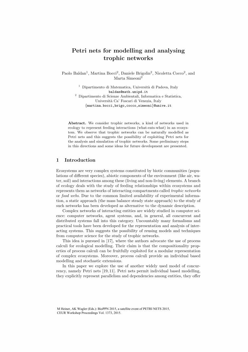
In our case study, the structural Petri net model has an Hilbert basis consist-ing of 69 minimal T-invariants, nine are internal and sixty are I/O invariants. Theinternal T-invariants are shown in Table 1. The first two invariants describe theself-predation (cannibalism) of MEZ and MIZ. All the other T-invariants “tra-verse” the DET place, pointing out that Detritus is the way for recycling matterin this network. The I/O invariants start from source transitions CO2 PHPand input DET and end in sink transitions PHP CO2, BPL CO2, MIZ CO2,MEZ CO2, TAP CO2 and TAP harvesting. They model trophic chains allowingfor respiration of the various compartments and for input and output of matter.

4.3 T-invariant based steady state

In this section we refine the structural Petri net model of a trophic network,turning it into a continuous Petri net model. What we obtain closely resemblesthe representation of the trophic network usually adopted by ecologists, where



Inv no. Transitions1 MEZ MEZ2 MIZ MIZ3 DET TAP; TAP DET4 DET BPL; BPL DET5 DET BPL; BPL MEZ; MEZ DET6 DET BPL; BPL MIZ; MIZ DET7 DET BPL; BPL TAP; TAP DET8 DET BPL; BPL MIZ; MIZ MEZ; MEZ DET9 DET BPL; BPL MIZ; MIZ TAP; TAP DET

Table 1. Internal minimal T-invariants of the structural Petri net model of TV .

the system is at a steady state and the input and output flows in all the compart-ments are balanced (the mass balance assumption). The choice of consideringa continuous extension is motivated by the fact that we are modelling fluxes ofbiomass which better correspond to continuous fluxes.

The continuous Petri net model is still derived only from the network topol-ogy by exploiting the minimal T-invariants in a way similar to what is done in[22] for Time Petri nets. A first observation is in order.

Remark 1. In the structural Petri net model of a trophic network Ns(T ) anyplace has typically at least one incoming and one outgoing transition, otherwisethe place would unnaturally correspond to a compartment with monotonicallyincreasing or decreasing content. Under this assumption, Ns(T ) is covered byT-invariants, namely each transition in the Petri net belongs to at least oneminimal T-invariant. In fact, when we exclude interface transitions Ns(T ) isa state machine, hence for any transition, if we follow the predecessors andsuccessors we will get back to the transition itself (internal T-invariant) or to aninterface transition on both sides (I/O T-invariant).

In order to associate rates with the transitions, we assume that each subsys-tem corresponding to a minimal T-invariant

1. is active and2. performs all its transitions once per time unit.

The assumption that all minimal subsystems of an ecosystem are active is quitereasonable from an ecological viewpoint. On the contrary the assumption thatall subsystems perform all their transitions exactly once per time unit is ratherstrong and unrealistic. This is the simplest choice which can be taken in absenceof further information on the ecosystem. When additional knowledge is available,it could be integrated in the model, as shown in the next section.

Let us consider the structural Petri net model Ns(T ) of a trophic networkT as described in Section 4.1 and its Hilbert basis B(Ns(T )). According to theassumptions above, the rate of a transition t should depend on the numberof minimal invariants in which t occurs. Then, for the trophic network T , wedefine the simple continuous Petri net model Nc(T ) as the continuous Petri netobtained by considering the structural model Ns(T ) as underlying Petri net andby associating to each transition t a constant rate given by:


30 P Baldan et al.

rate(t) = |{Ii|Ii ∈ B(Ns(T )) ∧ t ∈ Ii}|.

With such rates, all the transitions in all the invariants in Nc(T ) are per-formed once in one time unit and the system is in a steady state. Moreover, sinceall transition arcs are 1-weighted, rates and flows per time unit coincide.

Remark 2. The continuous Petri net model of a trophic network satisfies themass balance assumption, namely, for all compartments the sum of ingoing andoutgoing fluxes coincide. This is an immediate consequence of the fact thatminimal T-invariants are simple cycles or paths. Hence, given a place p, for anyinvariant Ii that “crosses” place p, one token is added to p by a transition in Iiand one token is consumed by another transition in Ii, namely the flux flowingthrough p via Ii is balanced. This holds for any invariant crossing p and for anyp. Therefore, the input and output fluxes coincide for any place of the network.

In the simple continuous model Nc(T ), the system is represented in a steadystate, with the fluxes of biomass balanced in all compartments. This correspondsclosely to the ecologists representation of a trophic network as a snapshot of thesystem at steady state. Note that the continuous Petri net model Nc(T ), despitethe fact that it makes explicit some additional features, is still based only on thetopology of T : biomasses do not play a role in the definition of the rates.

For our case study, the continuous Petri net model resulting from the con-struction outlined above is shown in Figure 2, where each transition have anassociated rate. Note that all places are balanced. We would like to validateour simple continuous model by considering some basic ecological processes andcheck their plausibility from an ecological point of view. For each compartmentwe compute the throughput, namely the total amount of flux flowing per unit oftime, in order to measure the degree of activity of the compartment. Besides wecompute food consumption (total amount of ingested food per time unit), foodassimilation (amount of ingested food minus amount of faeces, per time unit),respiration and mortality as percentages of the consumption. Table 2 shows thethroughputs, the assimilation and respiration values as resulting from the modelcompared with those found in the literature.

The values derived from the simple continuous model are quite interesting.Considering the throughput, the various compartments are ordered as follows:

DET>PHP>BPL=TAP>MIZ>MEZ.

We may distinguish two main groups: lower trophic level compartments (DET,PHP and BPL), having higher throughput, and higher trophic level compart-ments (TAP, MIZ and MEZ), having lower throughput. This is coherent withthe general knowledge on metabolic and growth rates of the two different groupsof compartments under consideration.

Assimilation of the top compartment TAP is just over the maximum indi-cated in the literature, while assimilation requirements for MEZ and MIZ areperfectly met. However, MEZ assimilation is close to the lower bound of theindicated range. This is due to the fact that MEZ is a top level compartment



Fig. 2. Continuous Petri net model for the case study

in the network and no predators are modelled for it. This is a quite unrealisticassumption: in natural systems MEZ are actually preyed by other species, likefishes. By adding an external predation on MEZ, we found that its assimilationbecomes close to TAP and MIZ assimilation values.

Concerning respiration, TAP and MEZ satisfy the constraints found in theliterature, while MIZ and BPL are slightly below the indicated value. Respirationof PHP is instead largely below the lower bound of the indicated range. Thelow respiration flows for MIZ, BPL and PHP is caused by the fact that thereare only a few I/O minimal invariants involving these compartments. This is amisbehaviour of the simple continuous model, that must be somehow overcome.

Concerning mortality, for BPL it is irrelevant and this is in accordance withexperimental data (see discussion in Section 2). Mortality of PHP is insteadquite high: this is probably due to the fact that some PHP grazers, like fishesusually occurring in lagoon systems, are not modelled.

On the whole, the continuous Petri net model realistically reproduces themain processes of the trophic network considered in the case study. Even if itbased only on the network topology, it allows for deriving some quantitativeinformation on trophic network flows, which are coherent with results of ex-perimental measures taken in natural ecosystems. Moreover, the quantitativevalidation shows that the model is somehow incomplete, signalling that two fur-ther predation fluxes, one for MEZ and one for PHP, should be represented inthe model.


32 P Baldan et al.

Compartment throughput Literature values Model valuesTAP 41 [25] Respiration ≥ 20% Respiration = 36%

[25] 37% ≤ Assimilation ≤ 70% Assimilation = 73%Defecation and Mortality = 27%

MEZ 28 [12] Respiration ≥ 20% Respiration = 37%[23, 9] 40% ≤ Assimilation ≤ 80% Assimilation = 39%

Defecation and Mortality = 61%MIZ 37 [12] Respiration ≥ 20% Respiration = 14%

[23, 9] 40% ≤ Assimilation ≤ 80% Assimilation = 78%Defecation and Mortality = 22%

BPL 41 [26, 5] Respiration ≥ 20% Respiration = 17%Assimilation = Consumption Assimilation = Consumption

Mortality = 2,4%PHP 49 [32, 3] 10% ≤ Respiration ≤ 30% Respiration = 2%

Assimilation = Consumption Assimilation = ConsumptionMortality = 22%

DET 58 not relevant not relevant

Table 2. Literature values and measured values for the continuous Petri net model ofthe case study.

4.4 Introducing ecological constraints in the Petri net model

In the previous section we underlined some misbehaviours of the simple continu-ous Petri net model. These are somehow expected since the model is only basedon the topology of the system and it relies on the strong assumption that allsubsystems proceed at the same speed. In order to adjust the model and makeit closer to the real trophic network, one can follow two directions:

1. Drop the assumption that all the subsystems perform their path exactly oncein one time unit and “speedup” some subsystems.

2. Use additional knowledge on the trophic network besides the topology, suchas the metabolism of the species or their diet, and impose some constraintson the rates of the corresponding transitions.

We next examine more closely these two alternatives and apply them to ourcase study.

Speeding-up subsystems. Recall that any linear combination of minimal T-invariantsis a T-invariant and a possible steady state of the network. Let us consider ageneric linear combination of all minimal T-invariants:∑

Ii∈B(Nc(T ))

kiIi , ki ∈ R.

The simple continuous model Nc(T ) corresponds to a steady state given bya linear combination of all the minimal T-invariants where all the ki are set toone. The refined continuous Petri net model, Ncs(T ), is obtained from Nc(T ) bydropping the assumption that all subsystems have the same speed and settingthe invariants constants ki to values possibly greater than one. In Ncs(T ) therate associated with each transition is generalised to:

rate(t) =∑

Ii∈B(Ns(T )), t∈Ii

ki.



rate after rate after rate afterNo. Transition rate speedup No. Transition rate speedup No. Transition rate speedup1 CO2 PHP 49 60 10 BPL MIZ 16 17 19 MEZ CO2 10 102 input DET 11 14 11 BPL TAP 11 11 20 TAP DET 11 113 PHP MIZ 20 22 12 MIZ MIZ 1 1 21 TAP CO2 15 154 PHP MEZ 10 10 13 MIZ DET 8 8 22 TAP Harv. 15 155 PHP DET 11 11 14 MIZ CO2 5 8 23 DET TAP 11 116 PHP TAP 7 7 15 MIZ MEZ 11 11 24 DET Export 7 77 DET BPL 41 44 16 MIZ TAP 12 12 25 PHP CO2 1 108 BPL CO2 7 9 17 MEZ MEZ 1 1 26 BPL DET 1 19 BPL MEZ 6 6 18 MEZ DET 17 17

Table 3. Rates of the continuous Petri net model before and after speedup.

The refined continuous Petri net model Ncs(T ) still represents the trophicnetwork at a steady state and with all compartments balanced, since the inputand output fluxes are balanced in each place for each minimal T-invariant.

We applied this idea to the case study and speed up the invariants involvingrespiration of PHP, BPL and MIZ, since the respiration flows of these compart-ments do not satisfy the ranges indicated in the literature (see Table 2). Thenew rates for the transitions are shown in Table 3.

Concerning PHP, it receives in input CO2 and partially release it for respira-tion. The unique I/O T-invariant for this process is {CO2 PHP; PHP CO2}. Byspeeding up this invariant to run ten times per unit of time, the respiration flowfor PHP becomes the 16% of its total consumption, within the range indicatedby the literature (see Table 2).

Concerning BPL, it is fed by the Detritus and part of the ingested food is usedfor respiration. The invariants involving transition BPL CO2 are {CO2 PHP;PHP DET; DET BPL; BPL CO2} and {input DET; DET BPL; BPL CO2}.By allowing the second invariant to run three times per unit of time, respirationof BPL become the 20% of its total consumption.

Concerning MIZ, we could speedup the invariants involving MIZ CO2, namely{CO2 PHP; PHP DET; DET MIZ; MIZ CO2} and {input DET; DET MIZ;BPL MIZ}. By allowing them to run three and two times per unit of time, re-spectively, respiration of BPL becomes the 20% of its total consumption. Assim-ilation of BPL becomes the 80% of the consumption, still in the range indicatedin Table 2.

Including constraints in the model. The second alternative for improving themodel consists in “embedding” into the continuous Petri net model of the trophicnetwork some available information regarding the metabolism of the speciesor their diet. We work under the simplifying assumption that flux constraintsimposed on the model are linear. This assumption is generally satisfied by theconstraints on metabolic fluxes and on the diet partitions. For our case study,some metabolic constraints taken from the literature are given in Table 2.

We define a continuous Petri net model which structurally coincides withNs(T ) and whose transition rates satisfy a set of linear inequalities. As in theprevious cases, the transition rates are derived from the “speed” ki of eachminimal invariant, but now we are interested only in invariants that satisfy the


34 P Baldan et al.

constraints. These can be obtained as solutions of a system of inequalities

AN ·X = 0C ·X ≥ 0

(1)

where AN is the incidence matrix of Ns(T ). We can consider the minimal suchT-invariants, referred to as the constrained Hilbert basis BC(Ns(T )), so that anysolution of (1) will be a linear combination of elements in BC(Ns(T )).

A continuous Petri net model Nc(T , C) for the trophic network T satisfyingthe constraints C is defined as follows. The underlying Petri net is Ns(T ) andeach transition t is associated with a constant rate:

rate(t) = |{Ii : Ii ∈ BC(Ns(T )) ∧ t ∈ Ii}|.

In this way each transition in each constrained invariant Ii in BC(Ns(T )) canbe performed once in one time unit.

When applied to our case study, this approach produces a linear system ofequalities and inequalities, where the inequalities express the literature knowl-edge summarised in Table 2. By considering only the inequalities given by thelower bounds, the constrained Hilbert basis contains 349 minimal invariants. Theinduced rate constants for the extended network automatically satisfy the givenecological constraints.

The two approaches could be combined, by determining the constrained in-variants and by setting for them possibly different speeds.

Simulations on continuous models with constant rates do not provide mean-ingful information. Some hints on how to further refine the model to do simula-tion analyses are given in the conclusions.

5 Conclusions and Future Work

In this paper we explored the use of Petri nets for representing and analysingtrophic networks and our preliminary results are encouraging. A trophic networknaturally translates into a structural Petri net model which allows for recoveringclassical trophic networks concepts and analyses. The structural model can berefined into a continuous Petri net model that closely resembles the representa-tion of the trophic network usually adopted by ecologists, where the system is ata steady state and the input and output flows are balanced in all the compart-ments. Despite the fact that the Petri net models proposed are still simplistic(in particular, the continuous models have constant rates, independent of themasses), in our case study of the Venice lagoon, the analysis of the continu-ous Petri net model shows that it realistically reproduces the main ecologicalprocesses. Furthermore, it shows that the continuous Petri net model can befruitfully used for an early stage validation of the trophic network under study.Two refinements of the continuous Petri net are considered: the first is based ona fine tuning of the speed of the minimal T-invariants, while the second one isbased on a systematic embedding of some ecological knowledge expressed as lin-ear inequalities into the calculation of the Hilbert basis. This however might have



scalability problems, since the constraints increase the size of the Hilbert basis,and the problem of determining the Hilbert basis is already in EXPSPACE.

Future work deals with making the Petri net model more realistic and dy-namic, by adding biomass information on compartments. The knowledge ofbiomasses at a steady state can, in fact, be used to derive constants for a con-tinuous model governed, e.g., by the mass action equation. We believe that in-troducing rates dependent on biomasses could allow for interesting simulations,describing, not only the steady state but also the transient behaviour leadingto such state. Additionally, on such model perturbations of the biomasses andof the speed of the various interactions could be used for performing what-ifanalyses.

Acknowledgements. We are grateful to Monika Heiner and Andrea Marin formany inspiring discussions.

References

1. 4ti2 team. 4ti2—a software package for algebraic, geometric and combinatorialproblems on linear spaces. Available at www.4ti2.de.

2. S. Allesina and R. E. Ulanowicz. Cycling in ecological networks: Finn’s indexrevisited. Computational Biology and Chemistry, 28:227–233, 2004.

3. R.S.K. Barnes and R.N. Hughes. An introduction to Marine Ecology. Wiley, 1999.

4. D. Brigolin and R. Pastres. Influence of intra-seasonal variability of metabolicrates on the output of a steady-state food web model. In Jordan F. and JørgensenS.E., editors, Models of the Ecological Hierarchy: From Molecules to the Ecosphere,Developments in Environmental Modelling, pages 165–179. Elsevier, 2012.

5. C.A. Carlson, P.A. Del Giorgio, and G.J. Herndl. Microbes and the dissipationof energy and respiration: from cells to ecosystems. Oceanography, 20(2):89–100,2007.

6. V. Christensen. Ecopath a software balancing steady-state models and calculatingnetwork characteristics. Ecological modelling, 61:169–185, 1992.

7. V. Christensen and C. J. Walters. Ecopath with Ecosim: methods, capabilities andlimitations. Ecological modelling, 172(2):109–139, 2004.

8. V. Christensen, C. J. Walters, and D. Pauly. Ecopath with ecosim: a users guide.Fisheries Centre, University of British Columbia, Vancouver, 154, 2005.

9. R.J. Conover. Factors affecting the assimilation of organic matter by zooplanktonand the question of superfluous feeding. Limnology and Oceanography, 11(3):346–354, 2003.

10. J. Desel and J. Esparza. Free Choice Petri Nets. Cambridge University Press,2005.

11. J. Esparza and M. Nielsen. Decidability issues for Petri Nets - a survey. JournalInform. Process. Cybernet. EIK, 30(3):143–160, 1994.

12. Vezina A. F. and M. L. Pace. An inverse model analysis of planktonic foodwebs in experimental lakes. Canadian Journal of Fisheries and Aquatic Sciences,51(9):2034–2044, 1994.

13. M. Heiner, D. Gilbert, and R. Donaldson. Petri Nets for Systems and SyntheticBiology. In Proc. of SFM’08, volume 5016 of LNCS, pages 215–264. Springer, 2008.


36 P Baldan et al.

14. M. Heiner, M. Herajy, F. Liu, C. Rohr, and M. Schwarick. Snoopy a unifyingPetri net tool. In Proc. of Petri Nets 2012, volume 7347 of LNCS, pages 398–407.Springer, 2012.

15. M. Heiner, M. Schwarick, and J. Wegener. Charlie an extensible petri net analysistool. In Proc. of Petri Nets 2015, LNCS. Springer, 2015. to appear.

16. R. E. Heymans, J. J. Ulanowicz and C. Bondavalli. Network analysis of the southflorida everglades graminoid marshes and comparison with nearby cypress ecosys-tems. Ecological Modelling, 149:5–23, 2002.

17. F. Jordan, M. Scotti, and C. Priami. Process algebra-based computational toolsin ecological modelling. Ecological Complexity, 8(4):357–363, 2011.

18. I. Koch and M. Heiner. Petri nets. In B. H. Junker and F. Schreiber, editors,Analysis of Biological Networks, Book Series in Bioinformatics, pages 139–179.Wiley, 2008.

19. T. Murata. Petri Nets: Properties, Analysis, and Applications. Proceedings ofIEEE, 77(4):541–580, 1989.

20. E.P. Odum. The strategy of ecosystem development. Science, 164(3877):262–270,1969.

21. Petri nets tools. http://www.informatik.uni-hamburg.de/TGI/PetriNets/tools.22. L. Popova-Zeugmann, M. Heiner, and I. Koch. Timed Petri Nets for modelling and

analysis of biochemical networks. Fundamenta Informaticae, 67:149–162, 2005.23. Parsons T. R., Takahashi M., and Hargrave B. Biological oceanographic processes.

Pergamon Press, 1984.24. A. Schrijver. Theory of linear and integer programming. Interscience series in

discrete mathematics and optimization. Wiley, 1999.25. I. Sorokin and O. Giovanardi. Trophic characteristics of the manila clam. ICES

Journal of Marine Science, 52(5):853–862, 1995.26. Reinthaler T., Winter C., and Herndl G. J. Relationship between bacterioplankton

richness, respiration, and production in the Southern North Sea. Applied andenvironmental microbiology, 5(7):2260–2266, 2005.

27. R. E. Ulanowicz. A phenomenological perspective of ecological development.Aquatic Toxicology and Environmental Fate, 9:73–81, 1986.

28. R. E. Ulanowicz. Quantitative methods for ecological network analysis and itsapplication to coastal ecosystems. Treatise on Estuarine and Coastal Science,9:35–57, 2011.

29. D. van Oevelen, K. van den Meersche, F. R. Meysman, K. Soetaert, J. Middel-burg, and A. Vezina. Quantifying Food Web Flows Using Linear Inverse Models.Ecosystems, 13:32–45, 2010.

30. M. Vasconcellos, S. Mackinson, K. Sloman, and D. Pauly. The stability of trophicmass-balance models of marine ecosystems: a comparative analysis. EcologicalModelling, 100:125–134, 1997.

31. A.F. Vezina and T. Platt. Food web dynamics in the ocean. I. Best-estimates offlow networks using inverse methods. Marine Ecology - Progress Series, 42:269–287,1988.

32. R. G. Wetzel. Limnology. Lake and River Ecosystems. Elsevier, 2001.


petri nets for modelling and analysing trophic networksceur-ws.org/vol-1373/paper2.pdf · petri...

Documents