peter a.e.m. janssen research department · pdf fileshinﬁeld park, reading, rg2 9ax, england...

755

Notes on the maximum wave height

distribution.

Peter A.E.M. Janssen

Research Department

June 2015

Series: ECMWF Technical Memoranda

A full list of ECMWF Publications can be found on our web site under:

http://www.ecmwf.int/en/research/publications

Contact: [email protected]

c©Copyright 2015

European Centre for Medium-Range Weather Forecasts

Shinfield Park, Reading, RG2 9AX, England

Literary and scientific copyrights belong to ECMWF and are reserved in all countries. This publication

is not to be reprinted or translated in whole or in part without the written permission of the Director-

General. Appropriate non-commercial use will normally be granted under the condition that reference

is made to ECMWF.

The information within this publication is given in good faith and considered to be true, but ECMWF

accepts no liability for error, omission and for loss or damage arising from its use.

http://www.ecmwf.int/en/research/publications

Notes on the maximum wave height distribution.

Abstract

This memo discusses a number of updates of the present freak wave warning system (Janssen &

Bidlot, 2009) which will be introduced in cycle 41R1 of the IFS. The list of changes is given below

and they are discussed in more detail in the remainder of this memo. They are:

1. Finite skewness effects, related to bound waves are introduced, and their impact is verified.

2. In the derivation of the maximum wave height distribution it is assumed that subsequent events

are independent. In contrast, here it is assumed that subsequent wave groups are independent,

rather than the individual waves. The number of independent events follows by making use of

the average length of a group, which depends on the width of the spectrum.

A Monte Carlo simulation for linear waves shows that the above assumption of statistical indepen-

dence of wave groups is a good choice. In particular, there is a close agreement between the simulated

and the theoretical maximum wave height distribution.

1 Introduction.

Recently, there has been considerable progress in the understanding of the occurrence of freak waves, a

notion which was first introduced by Draper (1965). Freak waves are waves that are extremely unlikely

as judged by the Rayleigh distribution of wave heights (Dean, 1990). In practice this means that when

one studies wave records of a finite length (say of 10-20 min), a wave is considered to be a freak wave if

the local wave height H (defined as the distance from crest to trough) exceeds the significant wave height

HS by a factor 2. It should be clear that it is hard to collect evidence on such extreme wave phenomena

because they occur so rarely. Nevertheless, observational evidence from time series collected over the

past decades does suggest that for large surface elevations the probability distribution for the surface

elevation may deviate substantially from the one that follows from linear theory with random phase,

namely the Gaussian distribution (cf. e.g. Wolfram and Linfoot, 2000). Also, there are now a number of

recorded cases which show that the ratio of maximum wave height and significant wave height may be

as large as three (Stansell, 2005).

Our increased understanding of the occurrence of extreme events is based on weakly nonlinear theory.

Extreme events are judged by means of the probability distribution function (pdf) of wave height and

maximum wave height. Although for linear waves the wave height pdf will be close to a Gaussian, finite

amplitude ocean waves may give rise to deviations from Normality. There are two reasons for it. First of

all, finite amplitude waves generate bound waves such as second and third harmonics which gives finite

skewness (connected with sharper crests and wider throughs) and kurtosis. The resulting deviations

from Normality will always occur as long as the waves are steep. However, there is another reason why

there may be large deviations from Normality but this will only occur when the sea state is coherent,

corresponding to a narrow spectrum in frequency and direction. Under those circumstances there is

possibly a strong four-wave interaction1 which may result in quite large amplitude waves corresponding

to large values of kurtosis and therefore to considerable deviations from Normality in such a way that

extreme events become more likely. Compared to the first reason, this dynamic mechanism is really

rare because it only occurs for nonlinear coherent sea states, but when it does occur it may cause large

1Extreme events can be simulated by means of the Zakharov equation (Zakharov, 1968, Janssen, 2003), which is the proto-

type equation for nonlinear four-wave interactions. Yasuda et al (1992), Trulsen and Dysthe (1997) and Osborne et al (2000)

studied simplified versions of the Zakharov equation and it was found that these extreme waves can be produced by nonlinear

self modulation of a slowly varying wave train. An example of nonlinear modulation or focussing is the instability of a uniform

narrow-band wave train to side-band perturbations. This instability, known as the Benjamin-Feir (1967) instability, will result

in focusing of wave energy in space and/or time as is illustrated by the experiments of Lake et al (1977).

Technical Memorandum No. 755 1


damage. This mechanism provides a plausible explanation for freak wave formation, which is definitely

a rare event.

In ocean wave forecasting practice one follows a stochastic approach because the phases of the individual

waves are unknown. In this memo we therefore concentrate on a probablistic approach, in particular we

try to utilize results from a random time series analysis. It is assumed that the wave spectrum E(ω) is

given and that we know relevant statistical moments such as the variance, the skewness and the kurtosis

of the time signal. Noting that maximum wave height is the parameter of first choice to characterize

extreme events, the important question then is whether it is possible to obtain a theoretical expression

for the maximum wave height distribution for given spectral shape and statistical moments, realizing

that a maximum parameter is defined for a given length of the time series. The answer to this question

depends on the choice of analysis technique: traditionally in the field of ocean waves one analyzes time

series in terms of wave height, defined through the zero-crossing method. In Janssen (2014) it is shown

that an alternative technique, namely use of the envelope of the time series, has certain advantages.

First, the square of the envelope gives a measure for the local (linear) energy of the waves, which is

a more interesting quantity then wave height if one is interested in the impact of waves on a marine

structure or a ship. Secondly, in linear theory it is straightforward to show that the probability distribution

function (pdf) of the envelope height follows the Rayleigh distribution, while no such simple pdf for the

zero-crossing wave height is known. Given the pdf for envelope wave height a theoretical expression

of maximum wave height is derived and this expression is validated against results from Monte Carlo

simulations.

The content of this memo is as follows. Using Monte Carlo Simulations for linear waves, in §2 a com-

parison is made between the pdf of wave height using the zero-crossing method and using the envelope

method. In agreement with theoretical results of Janssen (2014) it is found that the envelope wave height

obeys the Rayleigh distribution while the pdf of zero-crossing wave height depends on spectral shape

and only approaches the Rayleigh distribution from below for narrow spectra. We concentrate in §3 on

obtaining information about the occurrence of extreme events. To that end we try to derive, using the en-

velope method, the pdf of maximum wave height starting from the approach suggested by Goda (2000).

Given N independent events it is straightforward to obtain the probability that a time series has a given

maximum if the pdf of envelope wave height (which includes nonlinear effects as well) is known. The

key question is then how to estimate the number of independent events N. In §3 it is argued that succes-

sive wave groups may be regarded as independent so that the number of independent events will scale

with the ’average’ length of a wave group which is proportional to the product of the relative width of the

wave spectrum and the mean frequency. The maximum envelope wave height pdf will therefore depend

on spectral shape. This is confirmed by means of Monte Carlo simulations. Comparing the numerically

obtained pdf with the theoretical one for different spectral shapes a good agreement is obtained, sug-

gesting that with some confidence the thus developed theoretical approach may be used in estimating the

probability of extreme events. In §4 we extend the approach of §3 into the weakly nonlinear regime and

we show to what extend nonlinear effects may change the pdf of maximum wave height. In §5 of this

memo, after a discussion of the consequences for ECMWF’s freak wave warning system, a summary of

conclusions is presented.

2 Comparison of Envelope method and Zero-Crossing method.

It is common practice to analyze extreme ocean wave events by means of the zero-crossing method.

This is a very elegant method, which can be easily used and implemented. One just searches for two

consecutive zero-upcrossings in the time series and one determines the wave height from the difference

2 Technical Memorandum No. 755


of the maximum and the minimum of the surface elevation η in the corresponding time interval. Thus,

wave height is basically determined by sampling with the zero-crossing frequency (m2/m0)1/2 (where

mn is the nth moment of the spectrum), and to quantify the severity of the sea state one determines the

probability distribution function of the zero-crossing wave height. By applying the zero-crossing method

to time series of the surface elevation it turns out that the resulting pdf depends on spectral shape. This

follows from Monte Carlo simulations. In particular, for a narrow-band spectrum the zero-crossing wave

height pdf is found to be close to the Rayleigh distribution while for broad-band spectra extreme waves

are, when compared to the Rayleigh distribution, less likely to occur.

An alternative technique, based on the use of the envelope of the time series, shows a different picture.

I will call this alternative the envelope method. Although this method is not so popular in the field of

ocean waves it should be pointed out that in other fields, such as communication theory and nonlinear

optics, this approach is found to be very useful. Some aspects of the envelope method have been given in

Janssen (2014). The envelope ρ is obtained from the timeseries of the surface elevation η and its Hilbert

transform ζ = H(η), according to

ρ =√

η2 +ζ 2,

where for stationary signals surface elevation and its Hilbert transform have the same variance m0. The

local envelope wave height is then defined as Henv = 2ρ . In agreement with common practice in ocean

wave forecasting, wave height will be scaled with 4m1/2

0 so that we will study the statistical properties

of the dimensionless local wave height parameter h = Henv/4m1/2

0 . Theoretically and from Monte Carlo

simulations (see e.g. Janssen, 2014) one finds that for a Gaussian sea state the pdf of envelope wave

height follows the Rayleigh distribution, independent of spectral shape.

0 0.25 0.5 0.75 1 1.25 1.5 1.75 2 2.25 2.5h/hs

0.001

0.01

0.1

1

p(h

/hs)

MC Envelope (nu = 0.4)

Theory , Rayleigh

MC ZCM, nu = 0.40

MC ZCM, nu = 0.12

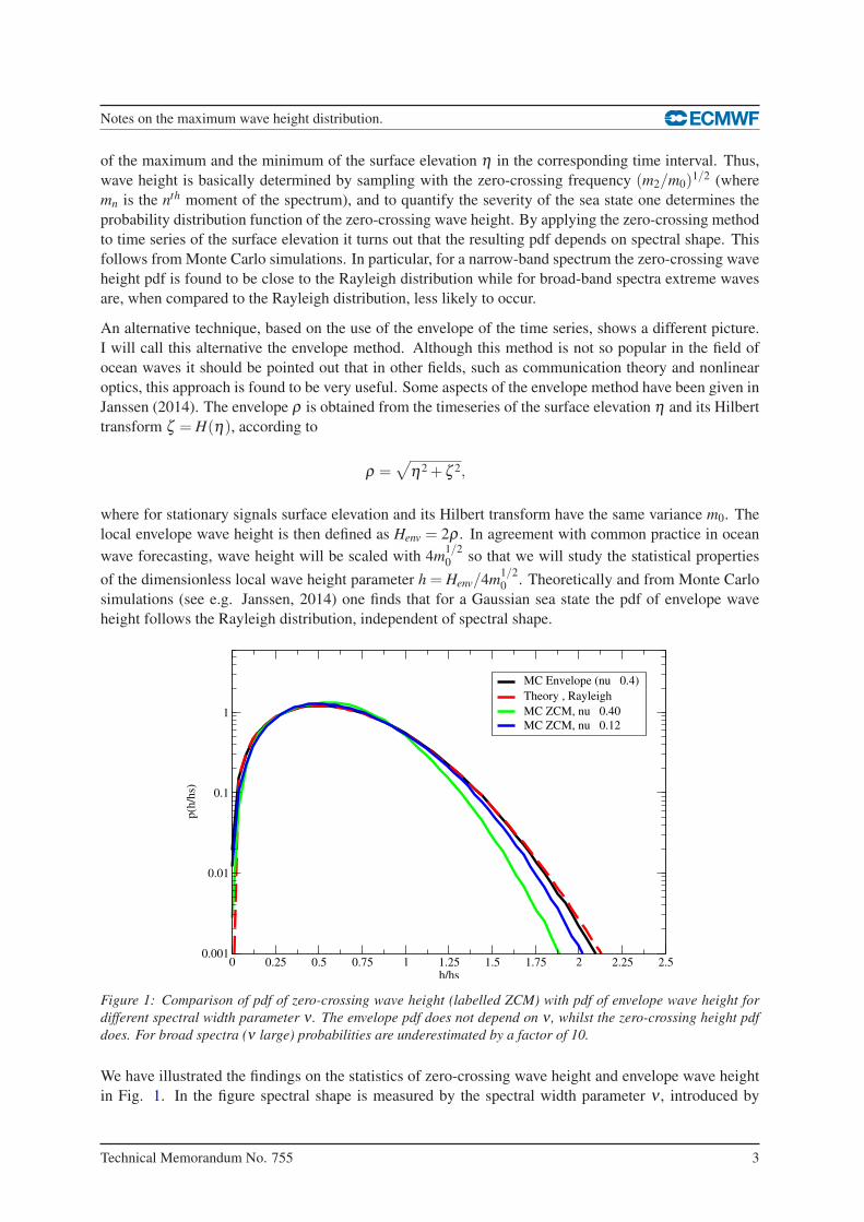
Figure 1: Comparison of pdf of zero-crossing wave height (labelled ZCM) with pdf of envelope wave height for

different spectral width parameter ν . The envelope pdf does not depend on ν , whilst the zero-crossing height pdf

does. For broad spectra (ν large) probabilities are underestimated by a factor of 10.

We have illustrated the findings on the statistics of zero-crossing wave height and envelope wave height

in Fig. 1. In the figure spectral shape is measured by the spectral width parameter ν , introduced by



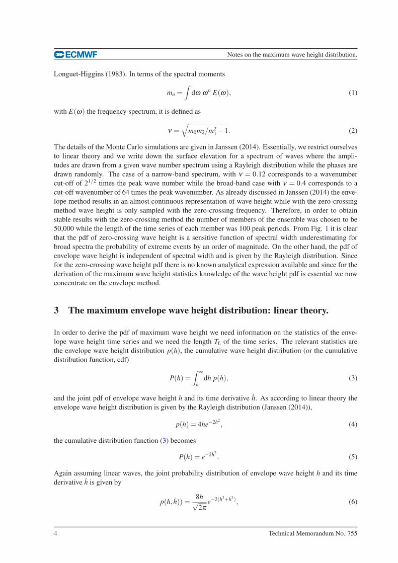
Longuet-Higgins (1983). In terms of the spectral moments

mn =∫

dω ωn E(ω), (1)

with E(ω) the frequency spectrum, it is defined as

ν =√

m0m2/m21 −1. (2)

The details of the Monte Carlo simulations are given in Janssen (2014). Essentially, we restrict ourselves

to linear theory and we write down the surface elevation for a spectrum of waves where the ampli-

tudes are drawn from a given wave number spectrum using a Rayleigh distribution while the phases are

drawn randomly. The case of a narrow-band spectrum, with ν = 0.12 corresponds to a wavenumber

cut-off of 21/2 times the peak wave number while the broad-band case with ν = 0.4 corresponds to a

cut-off wavenumber of 64 times the peak wavenumber. As already discussed in Janssen (2014) the enve-

lope method results in an almost continuous representation of wave height while with the zero-crossing

method wave height is only sampled with the zero-crossing frequency. Therefore, in order to obtain

stable results with the zero-crossing method the number of members of the ensemble was chosen to be

50,000 while the length of the time series of each member was 100 peak periods. From Fig. 1 it is clear

that the pdf of zero-crossing wave height is a sensitive function of spectral width underestimating for

broad spectra the probability of extreme events by an order of magnitude. On the other hand, the pdf of

envelope wave height is independent of spectral width and is given by the Rayleigh distribution. Since

for the zero-crossing wave height pdf there is no known analytical expression available and since for the

derivation of the maximum wave height statistics knowledge of the wave height pdf is essential we now

concentrate on the envelope method.

3 The maximum envelope wave height distribution: linear theory.

In order to derive the pdf of maximum wave height we need information on the statistics of the enve-

lope wave height time series and we need the length TL of the time series. The relevant statistics are

the envelope wave height distribution p(h), the cumulative wave height distribution (or the cumulative

distribution function, cdf)

P(h) =∫ ∞

hdh p(h), (3)

and the joint pdf of envelope wave height h and its time derivative h. As according to linear theory the

envelope wave height distribution is given by the Rayleigh distribution (Janssen (2014)),

p(h) = 4he−2h2

, (4)

the cumulative distribution function (3) becomes

P(h) = e−2h2

. (5)

Again assuming linear waves, the joint probability distribution of envelope wave height h and its time

derivative h is given by

p(h, h)) =8h√2π

e−2(h2+h2), (6)



where h has been normalized by means of the parameter m1/2

0 νω with ω = m1/m0 the mean angular

frequency while ν = (m0m2/m21 −1)1/2 is once more the width of the frequency spectrum. Note that by

considering the jpd of h and h the frequency scale νω is introduced in a natural way which corresponds

to the inverse of the relevant timescale of the wave groups. As time has been made dimensionless with

this frequency scale the length Tl of the timeseries has to be scaled accordingly, hence the dimension-

less length is T ∗L = TL × νω The result (6) is valid for a Gaussian sea state and can be obtained in a

straightforward manner from the well-known expression of the jpd of envelope ρ and phase φ and its

time derivatives (see e.g. Janssen (2014)). Integration over phase φ and its derivative φ and introduction

of the envelope wave height which is twice the envelope then results in (6).

3.1 Goda’s Approach.

Goda (2000) obtained the maximum wave height distribution from a time series of N independent wave

events assuming a narrow band wave train. The natural sampling frequency would be the mean zero

crossing frequency or perhaps the peak frequency as the length TL of the time series divided by the sam-

pling frequency would give the number of waves. A similar approach was already followed by Davenport

(1964) in the problem of estimating the maximum gust. In this note, we follow Goda’s (2000) approach

but now applied to time series of the envelope height. Clearly, when going from surface elevation to en-

velope height time series the mean oscillation frequency will be removed from our considerations which

will affect the sampling frequency. It will now involve the frequency scale νω . Note that this frequency

scale can be rewritten as νω = (m2/m0− ω2)1/2 which illustrates that for the envelope time series indeed

the mean oscillation frequency is removed from the signal.

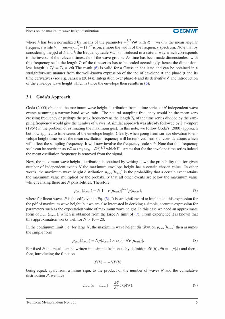
Now, the maximum wave height distribution is obtained by writing down the probability that for given

number of independent events N the maximum envelope height has a certain chosen value. In other

words, the maximum wave height distribution pmax(hmax) is the probability that a certain event attains

the maximum value multiplied by the probability that all other events are below the maximum value

while realizing there are N possibilities. Therefore

pmax(hmax) = N[1−P(hmax)]N−1 p(hmax), (7)

where for linear waves P is the cdf given in Eq. (3). It is straightforward to implement this expression for

the pdf of maximum wave height, but we are also interested in deriving a simple, accurate expression for

parameters such as the expectation value of maximum wave height. In this case we need an approximate

form of pmax(hmax), which is obtained from the large N limit of (7). From experience it is known that

this approximation works well for N > 10−20.

In the continuum limit, i.e. for large N, the maximum wave height distribution pmax(hmax) then assumes

the simple form

pmax(hmax) = N p(hmax)× exp[−NP(hmax)]. (8)

For fixed N this result can be written in a simple fashion as by definition dP(h)/dh =−p(h) and there-

fore, introducing the function

G (h) =−NP(h),

being equal, apart from a minus sign, to the product of the number of waves N and the cumulative

distribution P, we have

pmax(h = hmax) =dG

dhexp(G ). (9)



Close inspection of the result for the maximum wave height distribution shows that this distribution is a

double exponential function in general, but for large maximum wave heights (typically of the order of 2

or larger) the pdf simplifies considerable because it becomes

pmax(h) = N p(h).

This follows immediately from the basic result (7) and from the continuous limit (8) by realizing that

for extreme states the cdf P(hmax) is small. Using the cdf in (5) one finds that N times the cdf becomes

less than a small number, say ε , for the range h2 > 12

log(N/ε). For typical conditions with N = 100 and

ε = 0.01 one finds a threshold value slightly above 2.1, while for N = 10 the threshold value reduces to

1.8.

An important role in this approach is played by the parameter N which is a measure of the number of

independent events. It has been suggested (see e.g. Mori and Janssen, 2006) to equate N with the number

of waves N and therefore N = TL/Tp with TP the peak period and TL the length of the timeseries. This

may be a reasonable choice when the statistics of individual waves is considered but here we study the

properties of envelope time series. In the latter case it seems more natural to connect the number of

independent events with the number of wave groups (see e.g. Cramer and Leadbetter (1967) and Ewing

(1973)). This is the approach followed here and I will validate this choice using numerical evidence.

However, only a Gaussian sea state has been considered so far, therefore, for the estimation of the number

of degrees of freedom N skewness and kurtosis effects are ignored.

I find the estimation of the number of degrees of freedom not a trivial matter, and the following argument

only makes the choice (12) a plausible one. It is customary to define an event with respect to a chosen

reference level hc. An event is then a part of the time series that starts where the envelope has an

upcrossing and that finishes at the next downcrossing. The frequency of events is then determined by the

upcrossing frequency. The total number of events during the duration T ∗L then determines the number

of degrees of freedom N. For a more complete discussion see Elgar et al. (1984), where it follows that

N and also parameters such as the number of waves in a group depend on the chosen reference level,

but it is not clear which level to choose. Therefore, essentially the frequency of events depends on the

reference level, so it may be more appropriate to introduce an average frequency. The first measure of

frequency that came to mind is basically the average of the rate of change of h with time, h normalized

with h itself. Hence, the average frequency of events, determined by the average upcrossing frequency,

becomes

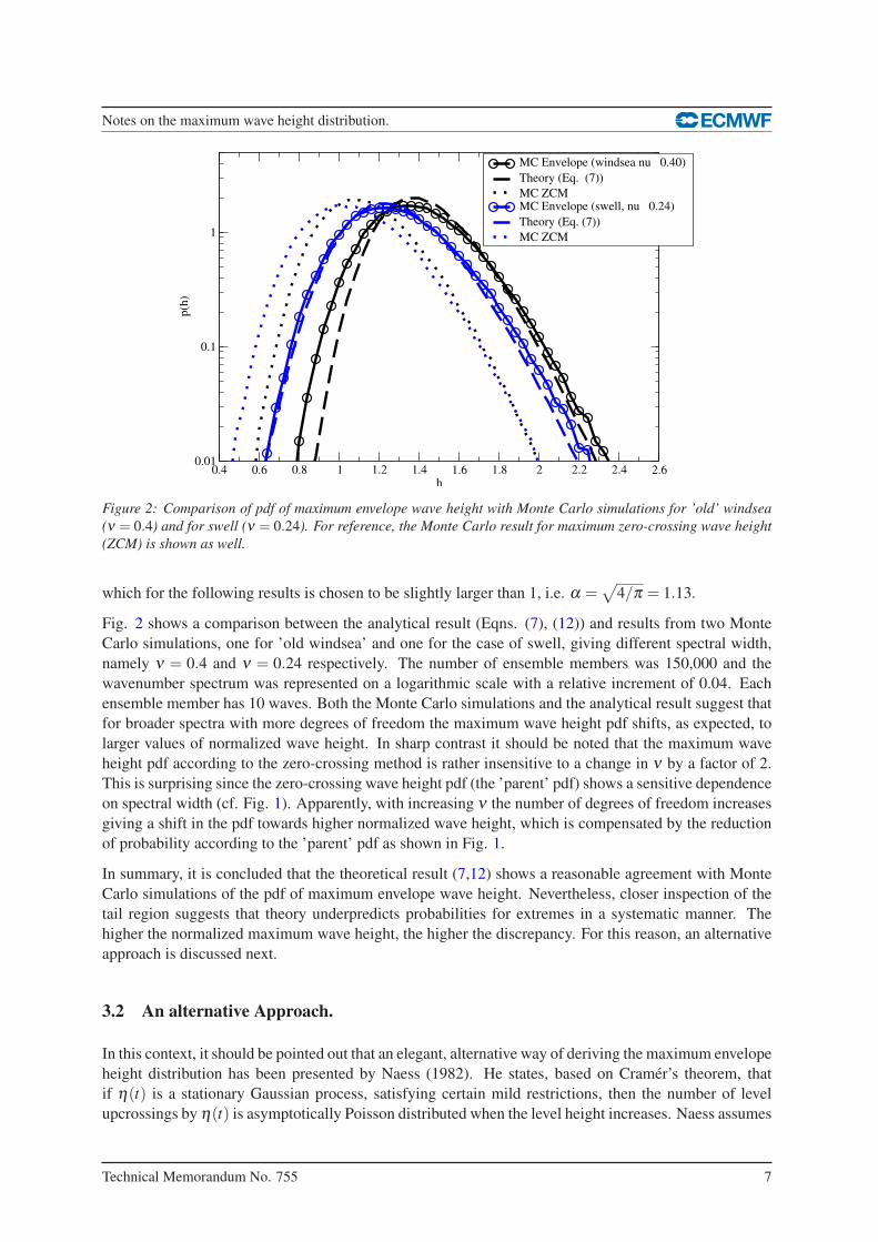
〈 fup〉= 〈h/h〉=∫ ∞

0dh

∫ ∞

0dh p(h, h) h/h (10)

Making use of the joint pdf of h and h in Eq. (6) and performing the integrations one immediately finds

the simple result

〈 fup〉= 1 (11)

and the average number of events becomes

N = 〈 fup〉T ∗L = νωTL.

This result reflects that the number of degrees of freedom is determined by the number of wave groups.

It is emphasized that I have only made plausible how N depends on the relevant parameters. To some

extent the result is uncertain because I have chosen to connect the number of events with the average

upcrossing frequency. For this reason I introduce a tuning coefficient α , hence

N = ανωTL. (12)



0.4 0.6 0.8 1 1.2 1.4 1.6 1.8 2 2.2 2.4 2.6h

0.01

0.1

1

p(h

)

MC Envelope (windsea nu = 0.40)

Theory (Eq. (7))

MC ZCMMC Envelope (swell, nu = 0.24)

Theory (Eq. (7))

MC ZCM

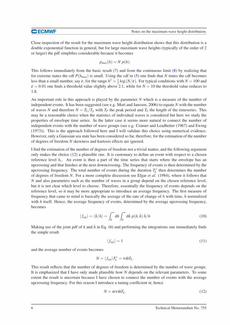
Figure 2: Comparison of pdf of maximum envelope wave height with Monte Carlo simulations for ’old’ windsea

(ν = 0.4) and for swell (ν = 0.24). For reference, the Monte Carlo result for maximum zero-crossing wave height

(ZCM) is shown as well.

which for the following results is chosen to be slightly larger than 1, i.e. α =√

4/π = 1.13.

Fig. 2 shows a comparison between the analytical result (Eqns. (7), (12)) and results from two Monte

Carlo simulations, one for ’old windsea’ and one for the case of swell, giving different spectral width,

namely ν = 0.4 and ν = 0.24 respectively. The number of ensemble members was 150,000 and the

wavenumber spectrum was represented on a logarithmic scale with a relative increment of 0.04. Each

ensemble member has 10 waves. Both the Monte Carlo simulations and the analytical result suggest that

for broader spectra with more degrees of freedom the maximum wave height pdf shifts, as expected, to

larger values of normalized wave height. In sharp contrast it should be noted that the maximum wave

height pdf according to the zero-crossing method is rather insensitive to a change in ν by a factor of 2.

This is surprising since the zero-crossing wave height pdf (the ’parent’ pdf) shows a sensitive dependence

on spectral width (cf. Fig. 1). Apparently, with increasing ν the number of degrees of freedom increases

giving a shift in the pdf towards higher normalized wave height, which is compensated by the reduction

of probability according to the ’parent’ pdf as shown in Fig. 1.

In summary, it is concluded that the theoretical result (7,12) shows a reasonable agreement with Monte

Carlo simulations of the pdf of maximum envelope wave height. Nevertheless, closer inspection of the

tail region suggests that theory underpredicts probabilities for extremes in a systematic manner. The

higher the normalized maximum wave height, the higher the discrepancy. For this reason, an alternative

approach is discussed next.

3.2 An alternative Approach.

In this context, it should be pointed out that an elegant, alternative way of deriving the maximum envelope

height distribution has been presented by Naess (1982). He states, based on Cramer’s theorem, that

if η(t) is a stationary Gaussian process, satisfying certain mild restrictions, then the number of level

upcrossings by η(t) is asymptotically Poisson distributed when the level height increases. Naess assumes



0.4 0.6 0.8 1 1.2 1.4 1.6 1.8 2 2.2 2.4 2.6h

0.01

0.1

1

p(h

)


Theory (Eq. (7))

Naess (Eq. (13))

0.4 0.6 0.8 1 1.2 1.4 1.6 1.8 2 2.2 2.4 2.6h

0.01

0.1

1

p(h

)


Theory (Eq. (7))

Naess (Eq. (13))

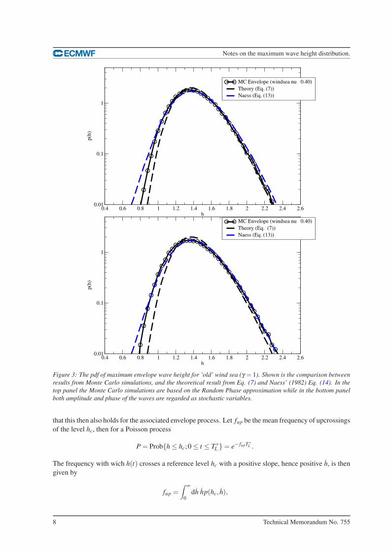
Figure 3: The pdf of maximum envelope wave height for ’old’ wind sea (γ = 1). Shown is the comparison between

results from Monte Carlo simulations, and the theoretical result from Eq. (7) and Naess’ (1982) Eq. (14). In the

top panel the Monte Carlo simulations are based on the Random Phase approximation while in the bottom panel

both amplitude and phase of the waves are regarded as stochastic variables.

that this then also holds for the associated envelope process. Let fup be the mean frequency of upcrossings

of the level hc, then for a Poisson process

P = Prob{h ≤ hc;0 ≤ t ≤ T ∗L }= e− fupT ∗

L .

The frequency with wich h(t) crosses a reference level hc with a positive slope, hence positive h, is then

given by

fup =∫ ∞

0dh hp(hc, h),



and substitution of (6) and carrying out the integration gives

fup =2hc√

2πe−2h2

c .

We now fix T ∗L and denote by H = max(h) for time t ∈ (0,T ∗

L ). Using this in the cdf P one finds

PH(h) = exp{−hNslce−2h2},

where PH denotes the probability distribution function of maximum wave height H, and,

Nslc = 2T ∗L /

√2π (13)

is the number of (up)crossings at the significant level h = 1. The maximum envelope height distribution

then follows from pmax(h) = dPH/dh, or,

pmax = (4h2 −1) Nslc e−2h2

PH(h), where h ≥ 1

2. (14)

The restriction h ≥ 12

is added in order to prevent the pdf from becoming negative. In addition, note that

the approach by Naess is only valid for large level crossings, presumably because it assumes that for

large levels the level upcrossings are statistically independent since these are rare events. An important

point to make is that in the present result the dependence of the average number of wave groups N on the

reference level has been taken into account, while in the result (8) N has been assumed a constant. As

a consequence, the large h behaviour of (14) differs from (8) because it involves an additional factor h.

Since we know that Eq. (8) underestimates probability in the tail of the distribution function I expect that

the present result might be more correct, in particular for high values of the maximum wave height. This

is born out by a comparison of (14) with simulations of the sea state with a Pierson-Moskovitz spectrum,

as shown in Fig. 3. However, it should be pointed out that this conclusion depends in a sensitive manner

on how the Monte Carlo simulations are being performed. Initially, simulations were done in such a way

that the amplitude of the waves is obtained in a deterministic manner from the wavenumber spectrum.

If the Monte Carlo simulations are performed in this manner the conclusion is that Goda’ approach

(7) shows a closer agreement with the numerical pdf than the result of Naess (14). This is shown in

the top panel of Fig. 3. But this method is strictly speaking not correct as the amplitudes are random

variables as well and, for a Gaussian sea state, should be drawn from a Rayleigh distribution. As a

consequence, following the last approach the numerical pdf tends to broaden and now Naess’ result is in

better agreement with the Monte Carlo result, as seen in in the bottom panel of Fig. 3, at least for the

extreme cases.

On the other hand, it should also be pointed out that for low wave height (i.e. h < 1/2) Naess’ approach

is not valid, as already mentioned before, and the pdf becomes negative, which is not really desirable.

The Goda approach does not suffer from this problem, and since probabilities for high waves are only

underestimated slightly I decided to continue with my original method (7,12).

3.3 Closing Remarks.

Before closing this Section I would like to mention two points. The first one is about an interesting

property of the pdf of maximum wave height which allows to estimate the number of degrees of freedom

from the observed/simulated maximum wave height pdf directly. The second point concerns the scaling

behaviour of the expectation value of maximum wave height with the number of degrees of freedom.



We have seen that under the extreme circumstances the maximum pdf is just N times the pdf of wave

height. Hence, the tail of the maximum wave height pdf just reflects the envelope wave height pdf and,

in fact, this provides an opportunity to estimate the number of degrees of freedom from the numerical

simulations by determining the ratio of simulated pdf, denoted by psimmax(h) and p(h) as a function of

dimensionless maximum wave height. When this quantity is plotted, as done in Fig. 4, then if the above

approach is correct one should expect a fairly flat ratio as function of maximum wave height while the

average value is then a good indicator for the magnitude of the number of degrees of freedom. In Fig.

0.6 0.8 1 1.2 1.4 1.6 1.8 2 2.2 2.4 2.6h

1

10

100

1000

N

N (Eq. (12))

Degrees of freedom using (4)

N_{slc} (Eq. (13))

Degrees of freedom using (14)

simulated R

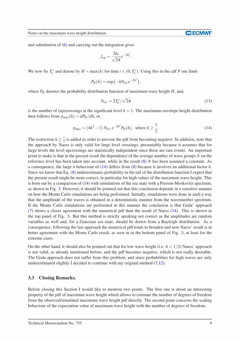
Figure 4: Estimate of the number of degrees of freedom N as function of maximum wave height h as obtained from

the ratio of simulated pdf psimmax(h) and p(h). The spectrum is for ’old’ windsea with γ = 1 with a truncation at 21/2

time the peak wave number and the length of the time series is 10 peak periods. The number of ensemble members

is 1,000,000. Two cases for the normalization are shown, one with p(h) given by (4) while also the result (14) of

Naess in the large N-limit is shown. Finally, the ratio R = psimmax(h)/psim(h), which is entirely based on simulation

results, as function of h is shown as the red line.

4 we show estimates of the number of degrees of freedom N as function of maximum wave height h

as obtained from the ratio R = psimmax(h)/p(h). In order to get a stable estimate in the tail of the pdf the

number of ensemble members was increased to 1,000,000 and, in order to save computation time, the

length of the time series was reduced to 10 waves. The spectrum is for ’old’ windsea with γ = 1 with

a truncation at 64 times the peak wave number. Two cases for the normalization are shown, one with

p(h) given by (4) while also the result using the normalization with the large h-limit of (14) is shown.

The thin black and blue lines are theoretical estimates of the degrees of freedom using, respectively,

the average number of upcrossings (12) or the number of upcrossings (Nslc of 13) corresponding to the

significant level h = 1. From the Figure it is suggested that Nslc is the appropriate choice for the number

of degrees of freedom, while the maximum wave height distribution (14) is in close agreement with

the numerical simulations since the estimated number of degrees of freedom is a flat function of h. It

seems, on the other hand, that the result from Goda’s approach (4) fits the numerical simulation less

comfortably, in particular for maximum wave heights above 2. Nevertheless, it should be realized that

by plotting the ratio R as function of dimensionless maximum wave height h one is really zooming in on

details of the tails of the distribution function. If one would, instead, plot the ratio R = psimmax(h)/psim(h)

(hence involving only simulation results) as a function of h, then it seems (see the red line in Fig. 4) that

Goda’s approach works equally well. Therefore, unfortunately, we cannot draw from this study a definite

conclusion on whether the Naess approach or Goda’s approach is to be preferred.

Up to now only a few cases have been considered and we studied in detail the shape of the maximum

wave height pdf, in particular its tail. Here we explore to what extent there is agreement for a wider



10 100 1000 10000N_{slc}

1

1.25

1.5

1.75

2

2.25

2.5

<h_m

ax>

Eq. (7) & (12)

Eq. (7) & (12)

MC; nu = 0.40

MC; nu = 0.12

MC (nu = 0.40) versus N_w

MC (nu = 0.12) versus N_w

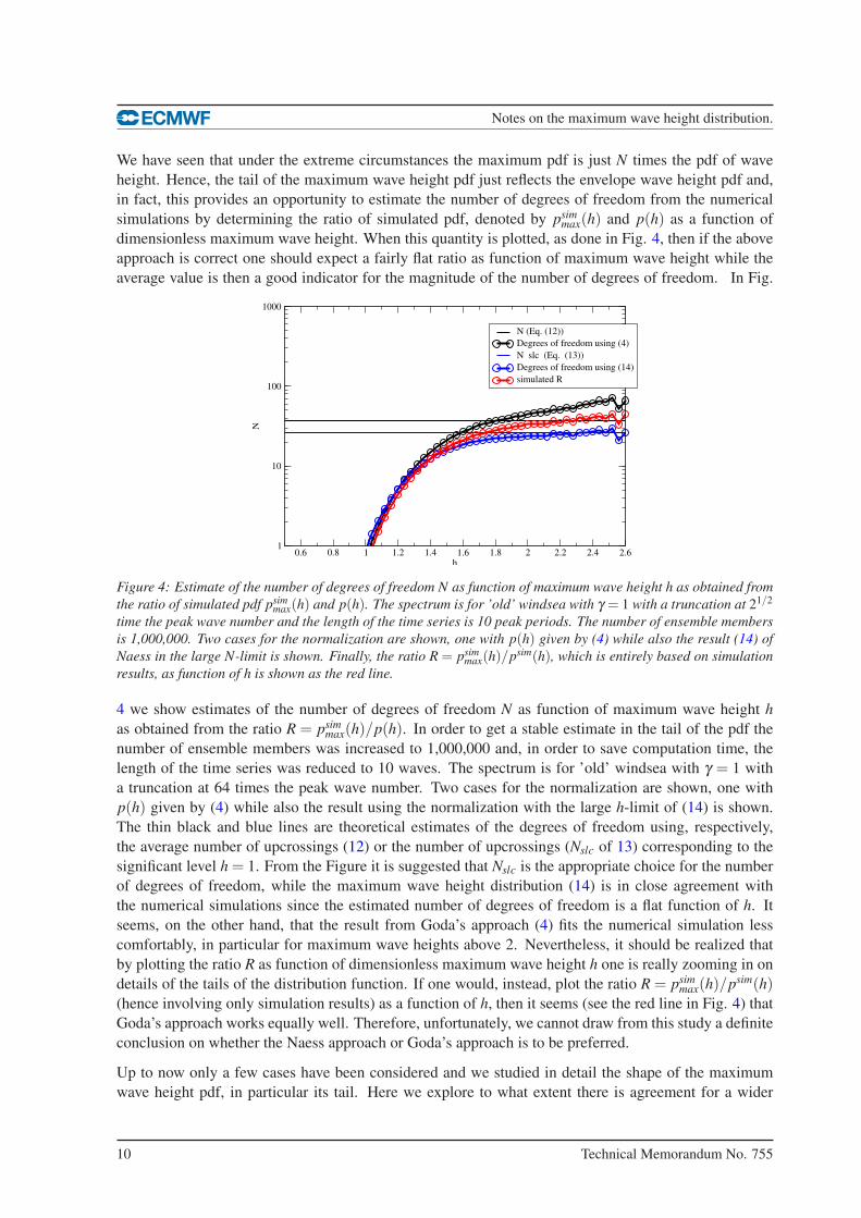
Figure 5: Expected maximum wave height versus number of upcrossings at the significant level (h=1) according

to the numerical simulations for two spectral widths. The green line shows the theoretical result based on Eq.

(7, 12).However, when results are plotted as function of the number of waves Nw = TL/TP (the blue symbols) no

scaling behaviour is found.

variety of cases but we restrict the comparison to the expectation value of maximum wave height, i.e.

〈h〉 = ∫

dh p(h). The expectation value of maximum wave height turns out to be a robust measure of

extreme seas, relatively insensitive to how the tail of the pdf is represented by the numerical simulation.

Therefore in order to produce the results displayed in Fig. 5 only 1,000 member ensembles were required.

In order to generate more cases we varied the number of waves in the timeseries from 50 to 500 and

we took two truncation limits, namely a wavenumber cut-off of 64 times the peak wave number and a

wavenumber cut-off of 21/2 times the peak wavenumber, representing a broad (ν = 0.40) and a narrow

(ν = 0.12) spectrum. In Fig. 5 we have plotted the expectation value of maximum wave height (a

key parameter to predict for extremes), as function of the number of upcrossings at the significant level

during the time interval TL (The number of degrees of freedom Nslc for short). From the comparison

between the Monte Carlo results and theory (Eqns. (7) and (12) it is clear that the agreement is excellent

and it seems that the suggested approach works for a wide range in the number of degrees of freedom,

even, surpisingly, for small values of Nslc. In addition, although we have chosen widely differing spectral

widths it is clear from the universal behaviour displayed in Fig. 5 that the choice νω for scaling of

the number of degrees of freedom is correct. An alternative choice, e.g. using the number of waves

N = TL/Tp (with Tp the peak period), does not give rise to proper scaling behaviour as is plainly evident

from the Figure.

4 Extension to weakly nonlinear waves.

Here, the work is presented to extend the probability for extreme wave height into the weakly nonlinear

regime. In particular, we concentrate on the pdf of maximum envelope wave height and it will be shown

how, given the statistics of envelope wave height (including nonlinear effects) the pdf of the maxima may

be obtained. Such an extension into the nonlinear regime is not so easy to obtain for the maximum zero

crossing wave height (at least I do not know how to do this), but a similar approach could be followed

for the maximum in surface elevation.

Janssen (2014) has obtained a new form for the pdf of wave height starting from the well-known Edge-



worth distribution. It reads

p(h) = 4he−2h2

{

1+κ4

8

(

2h4 −4h2 +1)

+κ2

3

72

(

4h6 −18h4 +18h2 −3)

}

. (15)

where

κ4 = κ40 +κ04 +2κ22.

and

κ23 = 5(k2

30 +κ203)+9(κ2

21 +κ212)+6(κ30κ12 +κ03κ21)

Here wave height is normalized with 4m1/2

0 where mn,n = 0,1,2, .. is the nth moment of the frequency

spectrum. Hence, h = 1 corresponds to the significant wave height level. The κ’s refer to certain third

and fourth-order cumulants of the joint pdf of the surface elevation and its Hilbert transform. They are

given in Janssen (2014) and in the present treatment they are assumed to be given, so the cumulants κ3

and κ4 are known. Assuming that the dynamics of the nonlinear waves is governed by nonlinear four-

wave interactions only, the even cumulants (for n > 0) consist of two contributions, namely one coming

from the bound waves and one coming from the dynamics of the free waves, while the odd cumulants

are determined by the presence of the bound waves only. The contribution by the free waves, however,

occurs very rarely because for it to be important a coherent sea state is required, i.e. one that has a

spectrum that is both narrow in frequency and direction. But when such a coherent sea state occurs large

deviations from Normality may result and it is then justified to call these sea states ’freakish’.

The difference with previous work is the additional term proportional to κ23 expressing the effect of

skewness on the pdf for (envelope) wave height. This is in particular relevant for the contribution of

bound waves to the deviations of statistics from Normality, as bound waves give rise to a considerable

skewness. On the other hand, it should be noted that the skewness of free waves is very small and

therefore for really extreme events the skewness correction to the wave height pdf is not so important.

However, on average, the bound waves will determine the statistics of waves and, therefore, in order to

have an accurate desciption of the average conditions the skewness effect needs to be included as well.

In order to derive the pdf of maximum wave height the cumulative wave height distribution

P(h) =∫ ∞

hdh p(h),

is required. Integration of p(h) from (15) gives

P(z) = e−2z[

1+κ4A(z)+κ23 B(z)

]

, (16)

with z = h2, while A(z) = z(z−1)/4 and B(z) = z(2z2−6z+3)/36. Because the cumulative distribution

function just depends on z = h2 it turns out that the most compact form of the maximum wave height

distribution is in terms of the linear wave energy parameter z. Hence, from Eq. (7) one obtains

pmax(z = h2max) =

dG

dzexp(G ), (17)

and once more G = −NP(z). The number of events N follows from (12), which for ease of reading is

displayed here once more, i.e.

N = ανωTL. (18)



Remark that strictly speaking one should estimate the number of degrees of freedom using the statistics

including nonlinear effects. This means extending the results displayed in Eqns. (8) and (10). This is

straightforward for the probability that the envelope wave height exceeds hc as the nonlinear extension

is given in Eq. (16), however, the nonlinear extension of the joint pdf of wave height h and its time

derivative h requires a substantial amount of additional work, which has not been done so far.

We have seen that the simplest description of the maxima pdf is in terms of the wave energy. It would

therefore be natural to evaluate the expectation value of maximum wave energy, i.e. 〈z〉. However,

since normally extreme seas are characterized by maximum wave height I will evaluate quantities such

as the expectation value of h and the width σ of the distribution. It will be found that the width σ of

the distribution function (17) is small, so the maximum wave height distribution is quite narrow, which

implies that 〈z〉1/2 and 〈z1/2〉 may be interchanged without much loss of accuracy.

The expectation value of maximum envelope wave height 〈h〉= 〈z1/2〉 can be found in the limit of large

N and small κ3 and κ4 in the following manner. By definition

〈h〉= 〈z1/2〉=∫ ∞

0dz z1/2 pmax(z).

Changing from integration variable z to x =−G and using the expression for the maximum wave height

distribution in (17) gives

〈h〉=∫ N

0dx z1/2(x)e−x. (19)

and z = z(x) is obtained by solving the relation between x and z, i.e.

x = Ne−2z(

1+κ4A(z)+κ23 B(z)

)

with a perturbation approach. Take the log and rearrange, then

z =1

2log

(

N

x

)

+1

2log

(

1+κ4A+κ23 B

)

and for small κ4 and κ3 one finds in good approximation

z = z0 +1

2log

(

1+κ4A(z0)+κ23 B(z0)

)

, z0 =1

2log

(

N

x

)

.

Now, utilizing that z0 is a large quantity, z1/2 becomes

z1/2 = z1/2

0 +1

4z1/2

0

log(

1+κ4A(z0)+κ23 B(z0)

)

, z0 =1

2log

(

N

x

)

. (20)

As a consequence, using (20) in (19) gives

〈h〉=∫ N

0dx

[

z1/2

0 +1

4z1/2

0

log(

1+κ4A(z0)+κ23 B(z0)

)

]

e−x = z1 + z2. (21)

Consider the first integral

z1 =∫ N

0dx z

1/2

0 e−x =1√2

∫ N

0dx e−x

√

logN − logx.



Because of the exponential function in the integrand contributions to the integral for x = O(N) are

exponentially small and therefore one may expand the square root term in the above integral as if logx is

small. As a result one finds

z1 ≃∫ ∞

0dx e−x

{

y0 −logx

4y0

}

.

with z0 =12

logN and y0 = z1/2

0 , while the upper bound N of the integral is replaced by ∞ as this also only

introduces an exponentially small term. According to Gradshteyn and Ryzhik (1965) one has∫ ∞

0dx e−x logx =−γ

where γ = 0.5772 is Euler’s constant and therefore

z1 = y0 +γ

4y0

Consider now the second integral in (21). Since this is a small contribution, the factor z0 may be replaced

by z0, and therefore

z2 =1

4y0

∫ N

0dx log

[

1+κ4A(z0)+κ33 B(z0)

]

e−x

Utilizing once more the assumption that κ23 and κ4 are small the logarithm is expanded. Elimination of

z0 and rearrangement then gives

z2 =1

4y0

(

ακ4 +βκ23

)

where

α =1

8

{

2z0(z0 −1)+(1−2z0)G1 +1

2G2

}

and

β =1

72

{

z0(4z20 −12z0 +6)− (6z2

0 −12z0 +3)G1 +3(z0 −1)G2 −1

2G3

}

,

where in the integrals the upper bound N has once more be replaced by ∞. The symbol Gn denotes

integrals involving exponentials and logarithms. These are related to the Gamma function Γ(1+ z) and

its derivatives,

Γ(1+ z) =∫ ∞

0tze−tdt =

∫ ∞

0ez log te−tdt,

and therefore

Gn =dn

dznΓ

∣

∣

∣

∣

z=0

=∫ ∞

0logn t e−tdt,n = 1,2,3, ...

It may be shown that G1 = Γ′(1) =−γ , G2 = Γ′′(1) = γ2+ π2

6, and G3 = Γ′′′(1) =−2ζ (3)−γ3−γπ2/2.

Here, ζ (3) = 1.20206 is the Riemann zeta function with argument 3. Now, returning to the logarithmic

form and combining the results for z1 and z2 one finds for 〈h〉

〈h〉= y0 +1

4y0

{

γ + log[

1+α(z0)κ4 +β (z0)κ23

]}

, (22)



The analytical result has been compared with results of numerical computations of 〈h〉 and the agreement

is astonishingly good. Notice that the assumption has been made that skewness and kurtosis are small, in

agreement with the assumptions on weakly nonlinear waves. Therefore, in the operational model, when

〈h〉 is computed, the kurtosis is restricted to the range −0.33 < 18κ4 < 1.

Next, a sketch is given of how the width σ of the maximum wave height distribution has been obtained.

By definition

〈z〉= σ2 + 〈h〉2,

therefore the expectation value of z denoted by 〈z〉 and defined as

〈z〉=∫ N

0dx ze−x =

∫ N

0dx e−x

{

z0 +1

2log

[

1+κ4A(z0)+κ23 B(z0)

]

}

is needed. The integrations can be performed in a similar fashion as before, and for linear waves (i.e.

κ3 = κ4 = 0) the relative width σ/〈h〉 becomes

σ

〈h〉 ≃π

2√

6(

logN + 12γ) .

For a typical choice of the number of waves, N = 100, the relative width is found to be around 13%.

The difference between 〈z〉1/2 and 〈z1/2〉 then turns out to be less than 1%. In this sense the maximum

wave height distribution is narrow, allowing the interchange of 〈z〉1/2 and 〈z1/2〉 without much loss of

accuracy.

1 1.25 1.5 1.75 2 2.25 2.5 2.75 3h

0.01

0.1

1

p(h

)

Nonlinear Theory (delta = 0.10)

Nonlinear Theory (delta = 0.05)

Linear Theory (delta = 0.0)

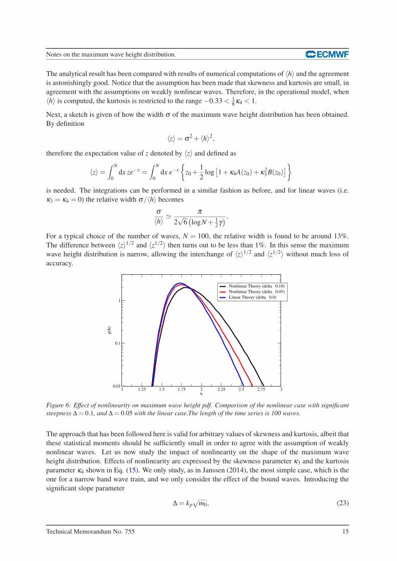
Figure 6: Effect of nonlinearity on maximum wave height pdf. Comparison of the nonlinear case with significant

steepness ∆ = 0.1, and ∆ = 0.05 with the linear case.The length of the time series is 100 waves.

The approach that has been followed here is valid for arbitrary values of skewness and kurtosis, albeit that

these statistical moments should be sufficiently small in order to agree with the assumption of weakly

nonlinear waves. Let us now study the impact of nonlinearity on the shape of the maximum wave

height distribution. Effects of nonlinearity are expressed by the skewness parameter κ3 and the kurtosis

parameter κ4 shown in Eq. (15). We only study, as in Janssen (2014), the most simple case, which is the

one for a narrow band wave train, and we only consider the effect of the bound waves. Introducing the

significant slope parameter

∆ = kp

√m0, (23)



one obtains for kurtosis and the square of the skewness

κ23 = 72∆2, κ4 = 24∆2. (24)

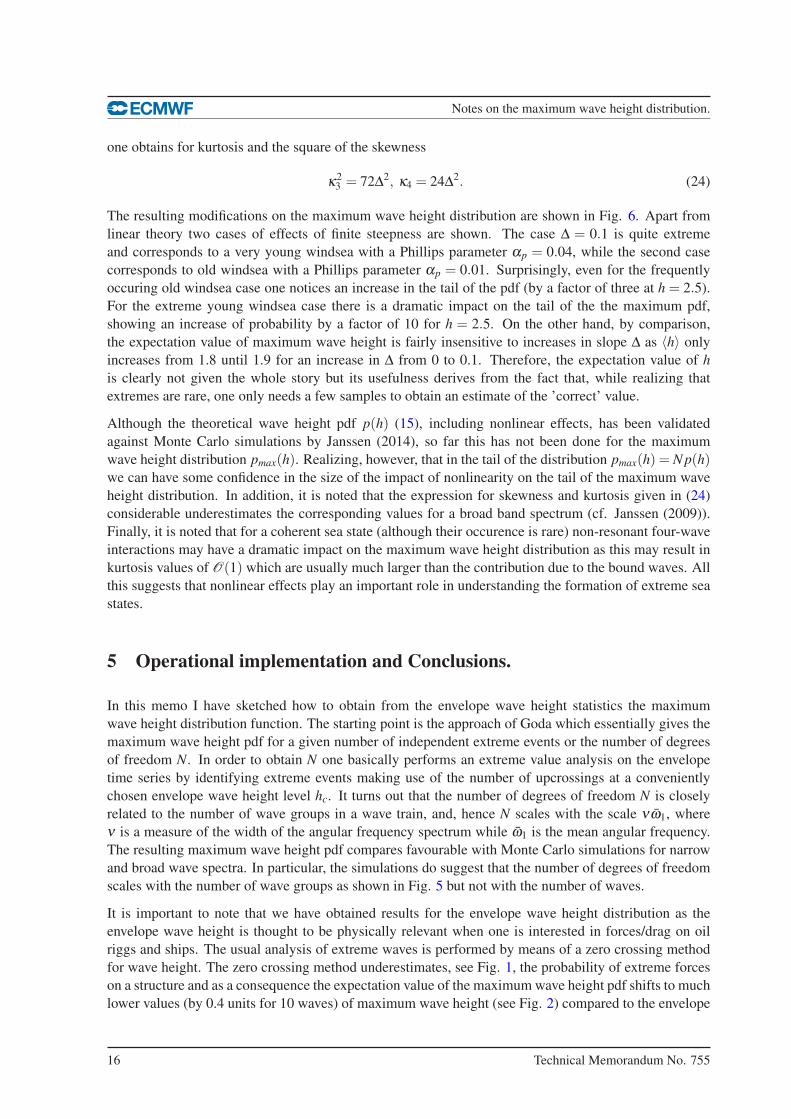
The resulting modifications on the maximum wave height distribution are shown in Fig. 6. Apart from

linear theory two cases of effects of finite steepness are shown. The case ∆ = 0.1 is quite extreme

and corresponds to a very young windsea with a Phillips parameter αp = 0.04, while the second case

corresponds to old windsea with a Phillips parameter αp = 0.01. Surprisingly, even for the frequently

occuring old windsea case one notices an increase in the tail of the pdf (by a factor of three at h = 2.5).

For the extreme young windsea case there is a dramatic impact on the tail of the the maximum pdf,

showing an increase of probability by a factor of 10 for h = 2.5. On the other hand, by comparison,

the expectation value of maximum wave height is fairly insensitive to increases in slope ∆ as 〈h〉 only

increases from 1.8 until 1.9 for an increase in ∆ from 0 to 0.1. Therefore, the expectation value of h

is clearly not given the whole story but its usefulness derives from the fact that, while realizing that

extremes are rare, one only needs a few samples to obtain an estimate of the ’correct’ value.

Although the theoretical wave height pdf p(h) (15), including nonlinear effects, has been validated

against Monte Carlo simulations by Janssen (2014), so far this has not been done for the maximum

wave height distribution pmax(h). Realizing, however, that in the tail of the distribution pmax(h) = N p(h)we can have some confidence in the size of the impact of nonlinearity on the tail of the maximum wave

height distribution. In addition, it is noted that the expression for skewness and kurtosis given in (24)

considerable underestimates the corresponding values for a broad band spectrum (cf. Janssen (2009)).

Finally, it is noted that for a coherent sea state (although their occurence is rare) non-resonant four-wave

interactions may have a dramatic impact on the maximum wave height distribution as this may result in

kurtosis values of O(1) which are usually much larger than the contribution due to the bound waves. All

this suggests that nonlinear effects play an important role in understanding the formation of extreme sea

states.

5 Operational implementation and Conclusions.

In this memo I have sketched how to obtain from the envelope wave height statistics the maximum

wave height distribution function. The starting point is the approach of Goda which essentially gives the

maximum wave height pdf for a given number of independent extreme events or the number of degrees

of freedom N. In order to obtain N one basically performs an extreme value analysis on the envelope

time series by identifying extreme events making use of the number of upcrossings at a conveniently

chosen envelope wave height level hc. It turns out that the number of degrees of freedom N is closely

related to the number of wave groups in a wave train, and, hence N scales with the scale νω1, where

ν is a measure of the width of the angular frequency spectrum while ω1 is the mean angular frequency.

The resulting maximum wave height pdf compares favourable with Monte Carlo simulations for narrow

and broad wave spectra. In particular, the simulations do suggest that the number of degrees of freedom

scales with the number of wave groups as shown in Fig. 5 but not with the number of waves.

It is important to note that we have obtained results for the envelope wave height distribution as the

envelope wave height is thought to be physically relevant when one is interested in forces/drag on oil

riggs and ships. The usual analysis of extreme waves is performed by means of a zero crossing method

for wave height. The zero crossing method underestimates, see Fig. 1, the probability of extreme forces

on a structure and as a consequence the expectation value of the maximum wave height pdf shifts to much

lower values (by 0.4 units for 10 waves) of maximum wave height (see Fig. 2) compared to the envelope



1.5 1.6 1.7 1.8 1.9 2 2.1 2.2 2.3Hmax/H_S

0

2.5

5

7.5

10

12.5

15

Norm

alis

ed d

istr

ibuti

on

Nonlinear Theory

Linear Theory

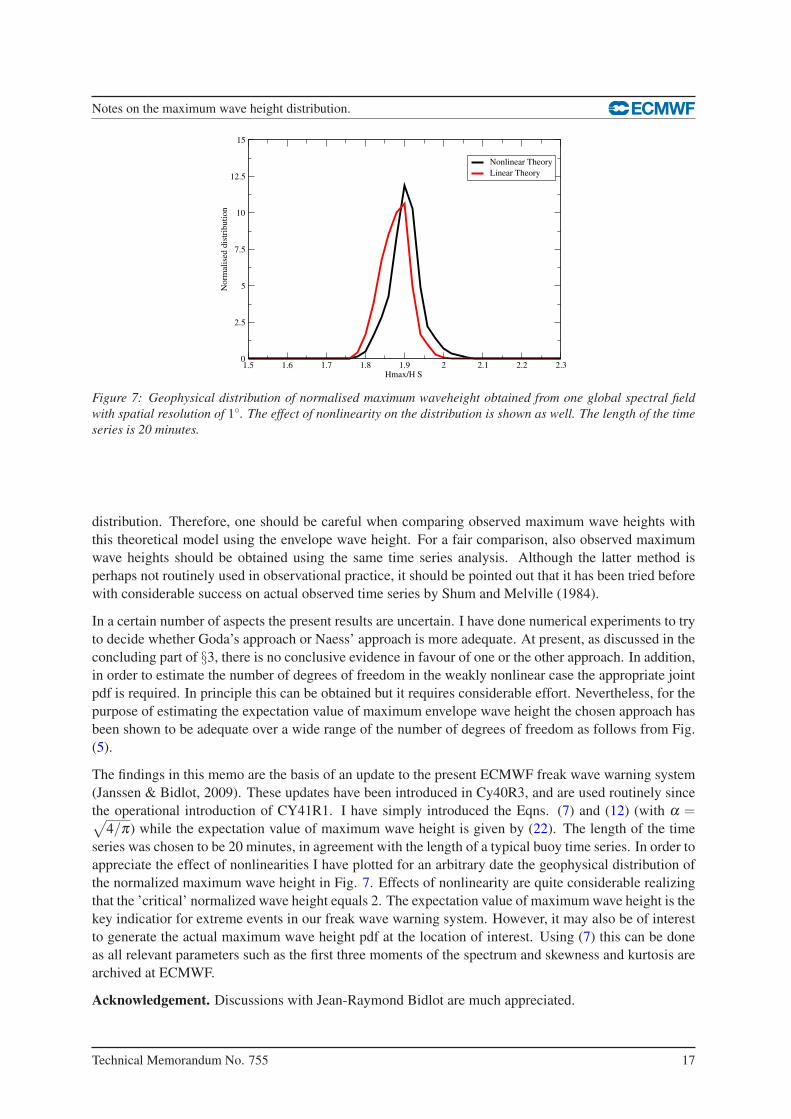
Figure 7: Geophysical distribution of normalised maximum waveheight obtained from one global spectral field

with spatial resolution of 1◦. The effect of nonlinearity on the distribution is shown as well. The length of the time

series is 20 minutes.

distribution. Therefore, one should be careful when comparing observed maximum wave heights with

this theoretical model using the envelope wave height. For a fair comparison, also observed maximum

wave heights should be obtained using the same time series analysis. Although the latter method is

perhaps not routinely used in observational practice, it should be pointed out that it has been tried before

with considerable success on actual observed time series by Shum and Melville (1984).

In a certain number of aspects the present results are uncertain. I have done numerical experiments to try

to decide whether Goda’s approach or Naess’ approach is more adequate. At present, as discussed in the

concluding part of §3, there is no conclusive evidence in favour of one or the other approach. In addition,

in order to estimate the number of degrees of freedom in the weakly nonlinear case the appropriate joint

pdf is required. In principle this can be obtained but it requires considerable effort. Nevertheless, for the

purpose of estimating the expectation value of maximum envelope wave height the chosen approach has

been shown to be adequate over a wide range of the number of degrees of freedom as follows from Fig.

(5).

The findings in this memo are the basis of an update to the present ECMWF freak wave warning system

(Janssen & Bidlot, 2009). These updates have been introduced in Cy40R3, and are used routinely since

the operational introduction of CY41R1. I have simply introduced the Eqns. (7) and (12) (with α =√

4/π) while the expectation value of maximum wave height is given by (22). The length of the time

series was chosen to be 20 minutes, in agreement with the length of a typical buoy time series. In order to

appreciate the effect of nonlinearities I have plotted for an arbitrary date the geophysical distribution of

the normalized maximum wave height in Fig. 7. Effects of nonlinearity are quite considerable realizing

that the ’critical’ normalized wave height equals 2. The expectation value of maximum wave height is the

key indicatior for extreme events in our freak wave warning system. However, it may also be of interest

to generate the actual maximum wave height pdf at the location of interest. Using (7) this can be done

as all relevant parameters such as the first three moments of the spectrum and skewness and kurtosis are

archived at ECMWF.

Acknowledgement. Discussions with Jean-Raymond Bidlot are much appreciated.



References

Benjamin, T.B., and J.E. Feir, 1967. The disintegration of wavetrains on deep water. Part 1. Theory. J.

Fluid Mech. 27, 417-430.

Cramer, H. and M.R. Leadbetter, Stationary and Related Stochastic Processes, John Wiley, New York,

1967.

Davenport, A.G., 1964. Note on the distribution of the largest value of a random function with application

to gust loading. Proc. Inst. Civil Engrs. 28, 187-196.

Dean, R.G., 1990. Freak waves: A possible explanation. In A. Torum & O.T. Gudmestad (Eds.), Water

Wave Kinematics (pp. 609-612), Kluwer.

Draper, L., 1965. ’Freak’ ocean waves. Marine Observer 35, 193-195.

Elgar, S., R.T. Guza and R.J. Seymour, 1984. Groups of Waves in Shallow Water. J. Geophys. Res. 89,

3623-3634.

Ewing, J.A., 1973. Mean length or runs of high waves. J. Geophys. Res. 78, 1933-1936.

Goda, Y., 2000. Random seas and Design of Maritime Structures. 2nd ed. World Scientific, 464 pp.

Gradshteyn, I.S. and I.M. Ryzhik, 1965. Tables of integrals, series, and products, Academic Press Inc,

New York and London.

Janssen, P.A.E.M., 2003. Nonlinear Four-Wave Interactions and Freak Waves. J. Phys. Oceanogr. 33,

863-884.

Janssen, P.A.E.M., 2009. Some consequences of the canonical transformation in the Hamiltonian theory

of water waves. J. Fluid Mech.637, 1-44.

Janssen, P.A.E.M., 2014. On a random time series analysis valid for arbitrary spectral shape, J. Fluid

Mech. 759, 236-256.

Janssen, P.A.E.M., and J.-R. Bidlot, 2009. On the extension of the freak wave warning system and its

verification. ECMWF Technical Memorandum 588.

Lake B.M., H.C Yuen, H. Rungaldier, and W.E. Ferguson, 1977. Nonlinear deep-water waves: Theory

and experiment. Part 2. Evolution of a continuous wave train, J. Fluid Mech. 83, 49-74.

Longuet-Higgins, M.S., 1983. On the joint distribution of wave periods and amplitudes in a random

wave field. Proc. Roy. Soc. London A389, 241-258.

Naess, A., 1982. Extreme value estimates based on the envelope concept. Applied Ocean research, 1982,

181-187.

Mori N. and P.A.E.M. Janssen, 2006. On kurtosis and occurrence probability of freak waves. J. Phys.

Oceanogr. 36, 1471-1483.

Osborne, A.R., M. Onorato, and M. Serio, 2000. The nonlinear dynamics of rogue waves and holes in

deep water gravity wave trains. Phys. Lett. A 275, 386-393.

Shum, K.T. and W.K. Melville, 1984. Estimates of the Joint Statistics of Amplitudes and Periods of

Ocean Waves Using an Integral Transform Technique. J. Geophys. Res. 89, 6467-6476.

Stansell, P., 2005. Distributions of extreme wave, crest and trough heights measured in the North Sea.



Ocean Engineering 32, 1015-1036.

Trulsen K., and K. Dysthe, 1997. Freak Waves-A Three-dimensional Wave Simulation. in Proceedings

of the 21st Symposium on naval Hydrodynamics(National Academy Press), pp 550-558.

Wolfram J., and B. Linfoot, 2000. Some experiences in estimating long and short term statistics for

extreme waves in the North Sea. Abstract for the Rogue waves 2000 workshop, Ifremer, Brest.

Yasuda, T., N. Mori, and K. Ito, 1992. Freak waves in a unidirectional wave train and their kinematics.

Proc. 23rd Int. Conf. on Coastal Engineering, Vol. 1, Venice, Italy, American Society of Civil Engineers,

751-764.

Zakharov, V.E., 1968. Stability of periodic waves of finite amplitude on the surface of a deep fluid. J.

Appl. Mech. Techn. Phys. 9, 190-194.


peter a.e.m. janssen research department · pdf fileshinﬁeld park, reading, rg2 9ax, england...

Documents