ARTICLE IN PRESS

Applied and Computational Mechanics 11 (2017) XXX–YYY

Periodic solutions of a graphene based model inmicro-electro-mechanical pull-in device

D. Weia,∗, S. Kadyrova, Z. Kazbeka

aDepartment of Mathematics, School of Science and Technology, Nazarbayev University, 53 Kabanbay Batyr Ave, Astana, 010000, Kazakhstan

Received 22 September 2016; accepted 13 April 2017

Abstract

Phase plane analysis of the nonlinear spring-mass equation arising in modeling vibrations of a lumped massattached to a graphene sheet with a fixed end is presented. The nonlinear lumped-mass model takes into accountthe nonlinear behavior of the graphene by including the third-order elastic stiffness constant and the nonlinearelectrostatic force. Standard pull-in voltages are computed. Graphic phase diagrams are used to demonstrate theconclusions. The nonlinear wave forms and the associated resonance frequencies are computed and presentedgraphically to demonstrate the effects of the nonlinear stiffness constant comparing with the corresponding linearmodel. The existence of periodic solutions of the model is proved analytically for physically admissible periodicsolutions, and conditions for bifurcation points on a parameter associated with the third-order elastic stiffnessconstant are determined.c© 2017 University of West Bohemia. All rights reserved.

Keywords: lumped-mass model, nonlinear spring, graphene, electrostatic pull-in stability, periodic solutions

1. Introduction

The importance of graphene can be highlighted in the title “The Arms Race for Graphene isOfficially On” of an article published in the Wall Stress Daily on May 21, 2014 [20]. Thepotential applications of graphene are everywhere [16]. Nanoscale engineering devices thatuse graphene as a material for basic components in resonators, switches, and valves are beingdeveloped in many industries [1, 4, 5, 12, 13, 23, 24]. Understanding the mechanical responsesof graphene structure elements subject to applied loads are clearly important, see e.g., [15],and above mentioned references. The use of graphene as an actuating cantilever beam subjectto electric pull-in force can be a major improvement over the use of the traditional pull-inmaterials, since graphene is more durable, stronger, and corrosion resistant, see e.g., [1,4,12,13].Many researchers have been using the linear constitutive equation in their models for graphenedevices, see [1, 4, 19, 23]. For example, a headphone equipped with a graphene membrane hasbecome a real life application of graphene [16, 23], however the mathematical model for themembrane reported in the work [23] considered graphene as a linear elastic material and alinear lumped parameter model based on Hooke’s law was used to estimate the frequenciesof vibrations. Nonetheless, the nonlinear mechanical behavior of graphene is well-known evenfor small strains and there are theoretical [2, 11, 15] and experimental [14] validations of thenonlinear mechanical behavior by using nonlinear constitutive equations. The widely acceptedcontinuum mechanics based nonlinear constitutive equation for graphene based materials in onedimensional form is given by

σ = Eε+D|ε|ε, (1)∗Corresponding author. Tel.: +771 727 099 368, e-mail: dongming.wei@nu.edu.kz.

https://doi.org/10.24132/acm.2017.322

1

D. Wei et al. / Applied and Computational Mechanics 11 (2017) XXX–YYY

where ε is the axial strain, σ is the axial stress, E is the Young’s modulus, and D = −E2/(4σmax)the third-order elastic stiffness constant, and σmax the ultimate yield stress of the graphene.Equation (1) is valid for |σ| ≤ σmax. It is demonstrated in [2] and [3] that the material constant Ddepends on the direction considered on the graphene plane.

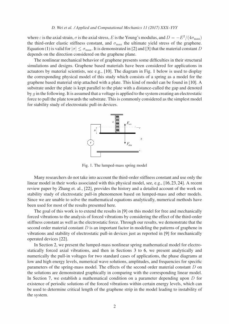
The nonlinear mechanical behavior of graphene presents some difficulties in their structuralsimulations and designs. Graphene based materials have been considered for applications inactuators by material scientists, see e.g., [10]. The diagram in Fig. 1 below is used to displaythe corresponding physical model of this study which consists of a spring as a model for thegraphene based material strip attached with a plate. This kind of model can be found in [10]. Asubstrate under the plate is kept parallel to the plate with a distance-called the gap and denotedby g in the following. It is assumed that a voltage is applied to the system creating an electrostaticforce to pull the plate towards the substrate. This is commonly considered as the simplest modelfor stability study of electrostatic pull-in devices.

Fig. 1. The lumped-mass spring model

Many researchers do not take into account the third-order stiffness constant and use only thelinear model in their works associated with this physical model, see, e.g., [16, 23, 24]. A recentreview paper by Zhang et. al., [22], provides the history and a detailed account of the work onstability study of electrostatic pull-in phenomenon based on lumped-mass and other models.Since we are unable to solve the mathematical equations analytically, numerical methods havebeen used for most of the results presented here.

The goal of this work is to extend the results in [9] on this model for free and mechanicallyforced vibrations to the analysis of forced vibrations by considering the effect of the third-orderstiffness constant as well as the electrostatic force. Through our results, we demonstrate that thesecond order material constant D is an important factor in modeling the patterns of graphene invibrations and stability of electrostatic pull-in devices just as reported in [9] for mechanicallyoperated devices [22].

In Section 2, we present the lumped-mass nonlinear spring mathematical model for electro-statically forced axial vibrations, and then in Sections 3 to 6, we present analytically andnumerically the pull-in voltages for two standard cases of applications, the phase diagrams atlow and high energy levels, numerical wave solutions, amplitudes, and frequencies for specificparameters of the spring-mass model. The effects of the second order material constant D onthe solutions are demonstrated graphically in comparing with the corresponding linear model.In Section 7, we establish a mathematical condition on a parameter depending upon D forexistence of periodic solutions of the forced vibrations within certain energy levels, which canbe used to determine critical length of the graphene strip in the model leading to instability ofthe system.

2

D. Wei et al. / Applied and Computational Mechanics 11 (2017) XXX–YYY

2. The nonlinear lumped-mass model

We assume that the cross-sectional area of the graphene sheet is Ac, one end of the sheet isfixed, and the other end is attached with a flat plate with mass m. The plate is subjected toa force F causing axial displacement of the graphene based material strip, which is mecha-nically modeled as a nonlinear spring. The axial displacement from equilibrium of the plateis denoted by x, the engineering strain is approximately modeled as x/L, where L is the len-gth of the graphene sheet. The restoring force of the spring is modeled by the restoring forceFres = −

(EAc

xL+DAc

∣∣ xL

∣∣ xL

)due to (1). By the Newton’s second law of motion, the vertical

displacement variable x in the lumped-mass nonlinear spring model shown in Fig. 1 satisfiesthe following nonlinear wave equation

md2xdt2+ EAc

x

L+DAc

∣∣∣xL

∣∣∣ x

L= Felec, (2)

where the constants E and D are the material constants appeared in (1).We wish to know how the solutions of nonlinear spring-mass model (2) responds to the

electrostatic force of the form Felec = ε0AV 2

2(g−x)2 and how important it is to include the thirdorder stiffness constant D in the graphene’s constitutive equation (1). In this case we have thefollowing spring-mass equation:

md2xdt2+ EAc

x

L+DAc

∣∣∣xL

∣∣∣ x

L=

ε0AV 2

2(g − x)2, (3)

where ε0 is the electric emissivity, V the applied voltage, and g the gap between the plate andthe substrate, Ac the cross-sectional area of graphene based material strip, A the area of theplate in the device illustrated by Fig. 1. For the derivation and physics and engineering aspect ofmodels similar to (2) with the electrostatic force Felec, see e.g., [21] and [17]. We remark that thismodel can be used for nonlinear materials similar to graphene with second order stress-strainresponses.

3. The pull-in voltages

The pull-in of the system is defined as the result of a sudden displacement of plate when theelectrostatic force overcomes the restoring force and the stiffness of the spring, causing the platephysically touch the substrate under it. The pull-in voltage is defined as the required voltagewhich causes the pull-in the spring-mass system. To find pull-in voltage for the model, weconsider the corresponding static equilibrium equation of (3): EAc

xL+ DAc

∣∣ xL

∣∣ xL= ε0AV 2

2(g−x)2

which can be solved for the pull-in voltage:

Vpull−in =

√2(g − x)2

(EAc

xL+DAc

∣∣ xL

∣∣ xL

)ε0A

. (4)

As it is pointed out in [7] that the pull-in occurs when the structure deflects to 2/3 of the initialgap g for a number of pull-in models. This statement has been experimentally and numericallyvalidated and reported in [6,8,18]. In this case, x = 2g/3 and the pull-in voltage of (3) is givenby

Vpull−in =2g9

√gEAc(3− 2α)

ε0AL, (5)

3

D. Wei et al. / Applied and Computational Mechanics 11 (2017) XXX–YYY

where α = −DgEL= Eg4σmaxL

. It is also assumed that pull-in can occur for many traditional pull-indevices when the structure deflects to 1/3 of the initial gap. In this case, we also have pull-in

voltage as Vpull−in =2g9

√2gEAc(3−2α)

ε0ALfor (3), see also, e.g., [5], for the assumptions leading to

these practices. The pull-in voltages corresponding to various plate areas and the two standardgap sizes are listed in Table 1.

Table 1. Pull-in voltages

Plate area Vpull−in (Volt) Vpull−in (Volt)A (μm2) at x = g/3 μm at x = 2g/3 μm160 000 37.27 52.48200 000 33.34 46.94250 000 29.82 41.98300 000 27.22 38.33

Adopted from [13], we use E = 1 000 GPa, Ac = 1 μm2, g = 2, L = 600 μm, andε0 = 8.85× 10−12 F/m for the permittivity of vacuum for numerical calculations of the pull-involtages. The results provided in Table 1 appear to be consistent with the values found in [5]and [13], where D is not included in the models.

4. Phase diagrams

For plotting the phase diagram and the bifurcation analysis, we will work with the followingdimensionless form of (3):

d2xdt2+ x − α|x|x = K

(x − 1)2 , (6)

where x = xg, t = t

√mLEAc

, K = ε0ALV 2

2EAcg3, α = −Dg

EL= Eg

Lσmax. For simplicity, we will still use x

and t to denote the x and t in (4). Multiply both sides of (6) by x and integrate the result relativeto t, we then have the conservation of energy equation

12(y2 + x2)− 1

3α|x|3 = K

1− x+ U0, (7)

where y = x and U0 is the integration constant.First, we provide numerical solutions for some specific values of K, g, L and U0 for plotting

the phase diagram of (6) by using (7). By using the change of variables, we can convert thephase diagrams of (6) to obtain the phase diagrams of (3). For simplicity, we only show thephase diagrams of (3) for some specific sets of parameters. The numerical phase diagramsare provided at different energy levels defined by the values of U0 to show the existence ofperiodic solutions and provide some further inside information about the existence of periodicsolutions. We plot diagrams for the voltage of 30 V which is lower than the pull-in voltage of37.27V for the plate with area that equals to 160 000 μm2. Several phase diagrams are presentedbelow to demonstrate the effect of the nonlinear term and the electrostatic force on the periodicsolutions.

4

D. Wei et al. / Applied and Computational Mechanics 11 (2017) XXX–YYY

(a) (b)

Fig. 2. Phase diagrams at low initial energy level

It can be seen from Fig. 2a–b that on both sides of the asymptote x = g = 2 there existperiodic solutions of (3) for some values of the initial energy level U0 and there is no periodicsolution for other values of U0. It is understood that the only periodic solutions on the leftare physically possible since the displacement x cannot be greater than the gap. Fig. 2b alsoindicates that above and near the point x = 2g/3 = 4/3, there is an unstable point which isconsistent with the findings in the literature [6–8] by some researchers.

(a) (b)

Fig. 3. Phase diagrams at high initial energy level

Fig. 3a shows the phase diagrams for higher levels of the initial energy U0. The impact ofthe nonlinear term α|x|x versus the effect of the electrostatic force term K/(g − x)2 on thephase diagram for (3) is also illustrated by Fig. 3, in which (a) corresponds to the case whenα|x|x dominates K/(g − x)2 and (b) to the opposite case. Our calculations indicate that thenonlinear restoring force term has stronger effects than the electrostatic force on the periodicsolutions. This seems to indicate that a full nonlinear analysis of the pull-in device is necessaryfor nonlinear materials with second order stress-strain responses.

5

D. Wei et al. / Applied and Computational Mechanics 11 (2017) XXX–YYY

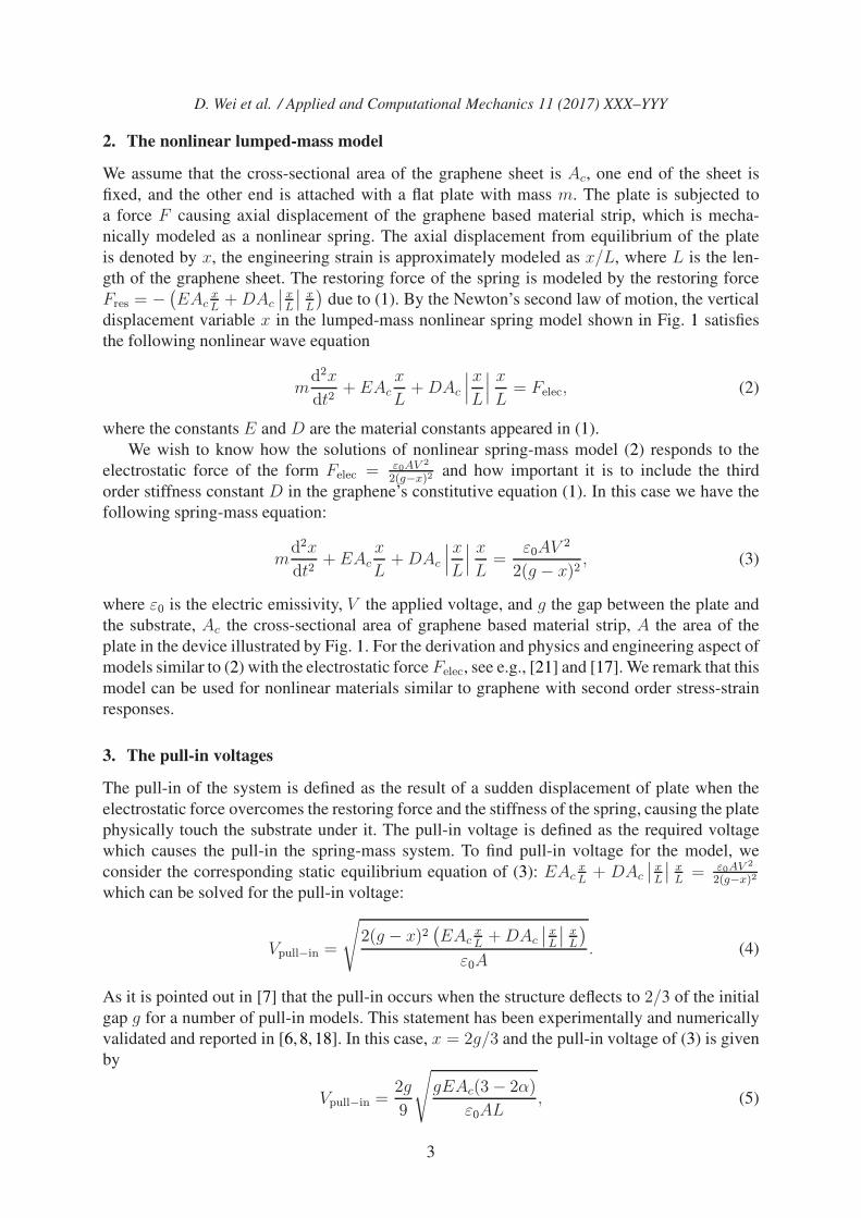
5. Numerical wave forms

In this section, we present graphic presentations of the periodic wave solutions. We use α =0.032 1, K = 0.038 23, x(0) = 0.3, x′(0) = 1 and α = 0.0, K = 0.038 23, x(0) = 0.3,x′(0) = 1, respectively, to obtain Fig. 4a for comparison of solutions of (3) with and withoutnonlinear stiffness effect. The nonlinear solution is slightly different than the linear solutionfor the same linear stiffness constant. Our numerical results also show how the nonlinearnumerical solution changes when the magnitude of the nonlinear term is increased significantly(by increasing the values of α, see Fig. 4b. Hence, we can suspect that the period increases asthe nonlinear term becomes bigger and frequency decreases as period goes up. It is clear thatthere is a bifurcation point, but it is not, for now, possible to find the general analytic expressionfor it. For particular values of parameters of the spring-mass system, numerical value of thebifurcation point may be computed. However, it is not practical to do this computation everytime, so we will establish a theoretical result later in Section 7 to determine such a bifurcationpoint.

Fig. 4. Comparison of waves of the linear model and the nonlinear model

Since we are unable to solve the mathematical equation (3) analytically, numerical methodsare used. The numerical technique adopted to solve the nonlinear differential equation (3) isbased on the Matlab function ode45, which uses the four stage Lobatto IIIA formula due to thegood stability properties of the procedure. The second-order nonlinear differential equation (3)is transformed by using �y = (x, x) into a first order system of the form dy

dt =�f(t, �y), which can

be solved by following the s-stage Runge-Kutta method that is, solving a system of nonlinearequations

�yi+1 − �yi − h

s∑j=1

βj�fj = 0, i = 1, . . . , N ; �y1 = (x(0), x(0)), (8)

where �fj = �f(ti + γih, �yi + h∑s

k=1 αjk�fk), �yi = �y(ti), i = 1, . . . , N , are the mesh points on

the time interval [0, T ∗], h is the step size. The number T ∗ > 0 is the chosen maximum time forthe numerical simulation. Different algorithms, such as Lobatto IIIA, are obtained by choosinga specific sets of values for parameters αi, βi and γi. See, e.g., the reference [18] for moredetails.

6

D. Wei et al. / Applied and Computational Mechanics 11 (2017) XXX–YYY

6. Periods and frequencies

Solving (7) for x and integrate the separable first-order ODE, converting to the dimensionalvariables in (7), we then obtain the integral formula to determine period and frequency

T = 4∫ 0

x∗

dx√−x2 + 2

3α|x|3 +2Kg−x+ 2U0

, (9)

where x∗ denotes the smallest x-intercept of the energy equation (7) in the phase plane in (x, y)and T denotes the period of the corresponding periodic solution. We assume that U0 = 1,V = 30 V, A = 160 000 μm2, and use the following sets of parameters:

L = 600 μm2, K = 0.382 3, and α = 0.003 21,L = 60 μm2, K = 0.382 3, and α = 0.003 21,L = 15 μm2, K = 0.009 557 5, and α = 0.128 5.

For the given three sets of values, we have the following values of the corresponding intercepts:1) x∗

1∼= −1.492 0, 2) x∗

2∼= −1.444 5 and 3) x∗

3∼= −1.518 2.

By using these values, we then integrate numerically the integrals and have the following threenumerical values of the periods for these three cases:

1) T1 ∼= 6.189 48, 2) T2 ∼= 6.367 34 and 3) T3 ∼= 6.854 31.It can be observed that as we increase the value of α from 0.003 21 to 0.128 4 (we incre-ase the effect of the nonlinear term), the corresponding period increases from 6.189 48 s to6.854 31 s. The frequencies can be found by the formula f = 1/T and we get f1 ∼= 0.161 56 s−1,f2 ∼= 0.157 05 s−1 and f3 ∼= 0.145 89 s−1.

7. Existence of periodic solutions and bifurcation analysis

In this section we discuss the existence of periodic solutions of (6) with initial conditions bystudying the graphs of the energy equation (7) for various values of the initial condition andthe parameter α. We assume that the initial conditions satisfy |y(0)| >

√2K and x(0) = 0.

Then, we have U0 = 12y(0)

2 − K > 0. The y-intercepts of the graph can be easily found to be±

√2(U0 +K). We consider the function

f(x) = −12x2 +

13α|x|3 + K

1− x+ U0, (10)

for finding a bifurcation point. Here, we demonstrate the existence of physically admissibleperiodic solutions of the forced vibrations within the gap g = 1 in the non-dimensional variable xand for certain initial energy levels U0 through the following Lemma and Proposition:

Lemma 1 There exists a physically admissible periodic solution if and only if f(x) = 0 forsome x ∈ (0, 1).Proof: We note that (7) defines a periodic solution of (6) if it defines a closed curve in the phasediagram. To be a physically admissible periodic solution it needs to be the closed curve around theequilibrium solution (0, 0) in the phase diagram. Since y = ±

√2f(x) and f(0) = K +U0 > 0

we see that for the equation defines a closed curve around (0, 0) there must exist x1 < 0 < x2 < 1such that f(x1), f(x2) ≤ 0. We note that for any x ∈ (0, 1) it holds that f(x) > f(−x) asK/(1 − x) > K/(1 − (−x)). Thus, the existence of x ∈ (0, 1) with f(x) = 0 immediately

7

D. Wei et al. / Applied and Computational Mechanics 11 (2017) XXX–YYY

implies the existence of x′ < 0 satisfying f(x′) = 0, since f(x) is continuous and f(0) = K+U0.Hence, it is necessary and sufficient to look at if f(x) = 0 for some x ∈ (0, 1).

In what follows, to simplify the notation we set H(x) = 3x2(1−x)−6(1−x)U0−6K2(1−x)x3 . We have the

following:

Proposition 1 Equation (6) has a physical periodic solution for some α ≥ 0 if and only if2U0 < 1 and H(x0) ≥ 0 for x0 = 1

3(1+√1 + 6U0). In fact, in this case, periodic solutions exist

for any α ∈ [0, H(x0)].Proof: In view of the Lemma 1, for given K, U0 > 0, we investigate the existence of a solutionof f(x) = 0 in the interval (0, 1) depending on the parameter α ≥ 0. As f(0) > 0 and f iscontinuous on [0, 1), we see that it suffices to find x ∈ (0, 1) such that f(x) ≤ 0. Solving for αfrom f(x) ≤ 0, we get α ≤ H(x). Therefore, the existence of x ∈ (0, 1) such that f(x) ≤ 0 isequivalent to the existence of x ∈ (0, 1) such that α ≤ H(x). Clearly, such a non-negative αexists if and only if h(x) ≥ 0 for some x ∈ (0, 1), where h(x) = (1−x)x2− 2(1−x)U0− 2K.Since, h(0) = −2(U0+K) < 0 and h(1) = −2K < 0, this is possible if and only if there exists acritical point of h(x) such that h(x0) ≥ 0. Taking the derivative, we have h′(x) = 2x−3x2+2U0,we see that h(x) has two critical points (1±

√1 + 6U0)/3 of which only x0 = (1+

√1 + 6U0)/3

is positive and it satisfies x0 < 1 if U0 < 1/2. Thus, we conclude that (7) has a closed curve, i.e.the equation (4) has a physically admissible periodic solution if and only if U0 < 1/2 as well ash(x0) ≥ 0. The latter is equivalent to H(x0) ≥ 0 which finishes the proof.

We now assume that U0 < 1/2 and H(x0) > 0. From Proposition 1, we see that α ≥ H(x0).Moreover, we see from Lemma 1 that if f(x) > 0 on (0, 1) then there are no admissible periodicsolutions. Clearly,

f(x) >12x2 − 1

3α|x|3 +K + U0 (11)

on (0, 1) and the right hand side function has the global minimum at x = 1/α on (0,∞). So, if− 12α2 +

α3α3 +K + U0 ≥ 0, we have no admissible periodic solutions.

Although our numerical phase diagrams indicate the existence of periodic solutions with|x(t)| > g, t ≥ 0, they are considered extraneous and physically impossible since they wouldbe below the line of the substrate in the model. Therefore, we omit the mathematical analysis ofthese cases.

8. Conclusion

A nonlinear spring-mass model for electrostatically forced axial vibration of a graphene ina simple pull-in device is presented following the work of [9]. The existence of periodicsolutions of free and forced vibrations is shown through phase plane analysis. Dependence ofthe periodic solutions to the model and bifurcation points on the parameter α = −Dg/(EL)is identified numerically. Pull-in voltages are calculated for different areas of the plate at twodifferent gap sizes. The analysis of phase diagrams demonstrates that, for high levels of theinitial energy, some unknown behaviors of the solutions are discovered which are distinct fromthose found in [9] which only considers mechanically forced vibrations. Numerical solutions ofsome periodic waves have been presented and the values of periods and frequencies for threedifferent values of length of the graphene are shown. Comparisons of the solutions with andwithout the presence of the second-order stiffness constant D = −E2/(4σmax) in the constitutivestress-strain equation for graphene are illustrated graphically and dramatic differences in thesesolutions are found. However, our results indicate that graphene behaves mechanically like all

8

D. Wei et al. / Applied and Computational Mechanics 11 (2017) XXX–YYY

the nonlinear continuum materials with 3rd order elastic stiffness. Among these materials, nographene-specific phenomena are found.

Acknowledgements

The authors thank the School of Science and Technology, Nazarbayev University for supportingcapstone research projects like the one that produced the part of results in this paper and alsothank the three anonymous reviewer’s valuable comments and suggestions which helped us toimprove the presentations in the paper significantly. The first author is thankful for the supportofthe Nazarbayev University ORAU grant which helped completing this paper.

References

[1] Atalaya, J., Isacsson, A., Kinaret, J. M., Continuum elastic modeling of graphene resonators, NanoLetters 8 (12) (2008) 4196–4200. https://doi.org/10.1021/nl801733d

[2] Cadelano, E., Palla, P. L., Giordano, S., Colombo, L., Nonlinear elasticity of monolayer graphene,Physical Review Letters 102 (2009) 1–4. https://doi.org/10.1103/PhysRevLett.102.235502

[3] Colombo, L., Giordano, S., Nonlinear elasticity in nanostructured materials, Reports on Progressin Physics 74 (2011) 116501 (1–35).

[4] Dai, M. D., Kim, C. W., Ecom, K., Nonlinear vibration behavior of graphene resonators andtheir applications in sensitive mass detection, Nanoscale Research Letters 7 (2012) 499–509.https://doi.org/10.1186/1556-276X-7-499

[5] Dequesnes, M., Rotkin, S. V., Aluru, N. R., Calculation of pull-in voltages for carbon-nanotube-based nanoelectromechanical switches, Nanotechnology 13 (2002) 120–131.https://doi.org/10.1088/0957-4484/13/1/325

[6] Ganji, B. A., Majlis, B. Y., Design and fabrication of a new MEMS capacitive microphoneusing a perforated aluminum diaphragm, Sensors and Actuators 149 (1) (2009) 29–37.https://doi.org/10.1016/j.sna.2008.09.017

[7] Ganji, B. A., Mousavi, A., Accurate determination of pull-in voltage for MEMS capacitive deviceswith clamped square diaphragm, IJE TRANSACTIONS B: Applications 3 (25) (2012) 161–166.

[8] Ganji, B. A., Nateri, M. S., Fabrication of a novel MEMS microphone using a lateral slotteddiaphragm, IJE TRANSACTIONS B: Applications 3 & 4 (23) (2010) 191–200.

[9] Hazim, H., Wei, D., Elgindi, M., Soukiassian, Y., A lumped-parameter model for nonli-near waves in graphene, World Journal of Engineering and Technology 3 (2015) 57–69.https://doi.org/10.4236/wjet.2015.32006

[10] Huang, Y., Liang, J., Chen, Y., The application of graphene based materials for actuators, Journalof Materials Chemistry 22 (2012) 3671–3680. https://doi.org/10.1039/c2jm15536b

[11] Lee, C., Wei, X., Kysar, J. W., Hone, J., Measurement of the elastic properties and intrinsic strengthof monolayer graphene, Science 321 (5887) (2008) 385–388.https://doi.org/10.1126/science.1157996

[12] Lin, W. H., Zhao, Y. P., Pull-in instability of micro-switch actuators: Model review, Inter-national Journal of Nonlinear Sciences and Numerical Simulation 9 (2) (2008) 175–183.https://doi.org/10.1515/IJNSNS.2008.9.2.175

[13] Liu, C., Analysis of electrostatic actuator, Lecture Notes, MASS UIUC, 2012.[14] Lu, Q., Huang, R., Nonlinear mechanics of single-atomic-layer graphene sheets, International

Journal of Applied Mechanics 1 (3) (2009) 443–467.https://doi.org/10.1142/S1758825109000228

[15] Malina, E. W. C., Mechanical behavior of atomically thin graphene sheets using atomic forcemicroscopy nano-indentation, M.S. Thesis, University of Vermont, 2011.

9

D. Wei et al. / Applied and Computational Mechanics 11 (2017) XXX–YYY

[16] Novoselov, K. S., A roadmap for graphene, Nature 490 (2012) 192–200.https://doi.org/10.1038/nature11458

[17] Rochus, V., Rixen, D. J., Golinval, J. C., Electrostatic coupling of MEMS structures: Transientsimulations and dynamic pull-in, Nonlinear Analysis 63 (2005) 1619–1633.https://doi.org/10.1016/j.na.2005.01.055

[18] Shampine, L. F. et al., Solving ODEs with MATLAB, Cambridge University Press, 2003.https://doi.org/10.1017/CBO9780511615542

[19] Suggs, M. E., Graphene resonators analysis and film transfer, Sandia Report, SAND2012-4433,Unlimited Release, 2012. https://doi.org/10.2172/1055606

[20] Williams, R., The arms race for graphene is officially on, Wall Street Daily, May 21, 2014.[21] Younis, M. I., MEMS linear and nonlinear statics and dynamics, Springer, 2011.

https://doi.org/10.1007/978-1-4419-6020-7[22] Zhang, W. M., Yan, H., Peng, Z. K., Meng, G., Electrostatic pull-in instability in MEMS/NEMS: A

review, Sensors and Actuators A 214 (2014) 187–218. https://doi.org/10.1016/j.sna.2014.04.025[23] Zhou, Q., Zettl, A., Electrostatic graphene loudspeaker, Applied Physics Letter 102 (2013) 223109.

https://doi.org/10.1063/1.4806974[24] Zhou, Q., Zettl, A., Electrostatic graphene speaker, WO2014100012 A1, Patent Application, 2014.

10