peridynamics with lammps: a user guide v0.1...
TRANSCRIPT

SANDIA REPORT2008-0135Unlimited ReleasePrinted July 2008
Peridynamics with LAMMPS:A User Guidev0.1 Beta
Michael L. Parks, Pablo Seleson, Steven J. Plimpton, Richard B. Lehoucq, andStewart A. Silling
Prepared bySandia National LaboratoriesAlbuquerque, New Mexico 87185 and Livermore, California 94550
Sandia is a multiprogram laboratory operated by Sandia Corporation,a Lockheed Martin Company, for the United States Department of Energy’sNational Nuclear Security Administration under Contract DE-AC04-94-AL85000.
Approved for public release; further dissemination unlimited.

Issued by Sandia National Laboratories, operated for the United States Department of Energy by SandiaCorporation.
NOTICE: This report was prepared as an account of work sponsored by an agency of the United StatesGovernment. Neither the United States Government, nor any agency thereof, nor any of their employees,nor any of their contractors, subcontractors, or their employees, make any warranty, express or implied,or assume any legal liability or responsibility for the accuracy, completeness, or usefulness of any infor-mation, apparatus, product, or process disclosed, or represent that its use would not infringe privatelyowned rights. Reference herein to any specific commercial product, process, or service by trade name,trademark, manufacturer, or otherwise, does not necessarily constitute or imply its endorsement, recom-mendation, or favoring by the United States Government, any agency thereof, or any of their contractorsor subcontractors. The views and opinions expressed herein do not necessarily state or reflect those ofthe United States Government, any agency thereof, or any of their contractors.
Printed in the United States of America. This report has been reproduced directly from the best availablecopy.
Available to DOE and DOE contractors fromU.S. Department of EnergyOffice of Scientific and Technical InformationP.O. Box 62Oak Ridge, TN 37831
Telephone: (865) 576-8401Facsimile: (865) 576-5728E-Mail: [email protected] ordering: http://www.osti.gov/bridge
Available to the public fromU.S. Department of CommerceNational Technical Information Service5285 Port Royal RdSpringfield, VA 22161
Telephone: (800) 553-6847Facsimile: (703) 605-6900E-Mail: [email protected] ordering: http://www.ntis.gov/help/ordermethods.asp?loc=7-4-0#online
DEP
ARTMENT OF ENERGY
• • UN
ITED
STATES OF AM
ERI C
A
2

2008-0135Unlimited ReleasePrinted July 2008
Peridynamics with LAMMPS:
A User Guide
v0.1 Beta
Michael L. Parks ∗ Pablo Seleson §
Steven J. Plimpton † Richard B. Lehoucq ∗
Stewart A. Silling ‡
∗Computational Mathematics and Algorithms†Scalable Algorithms
‡Multiscale Dynamic Material ModelingSandia National Laboratories
P.O. Box 5800Albuquerque, NM 87185-1320
§Dept. of Scientific Computing400 Dirac Science LibraryFlorida State University
Tallahassee, FL 32306-4120
Abstract
Peridynamics is a nonlocal formulation of continuum mechanics. The discrete peridynamicmodel has the same computational structure as a molecular dynamics model. This documentprovides a brief overview of the peridynamic model of a continuum, then discusses how theperidynamic model is discretized, and overviews the LAMMPS implementation. An exampleproblem is also included.
3

4

Contents
1 Introduction . . . . . . . . . . . . . . . . . . . . . . . . . . . . . . . . . . . . . . . . . . . . . . . . . . . . . . . . . . . . . . . . 91.1 Typographical Conventions . . . . . . . . . . . . . . . . . . . . . . . . . . . . . . . . . . . . . . . . . . . . . . . . 9
2 Getting Started. . . . . . . . . . . . . . . . . . . . . . . . . . . . . . . . . . . . . . . . . . . . . . . . . . . . . . . . . . . . . 102.1 Building the Peridynamic Module within LAMMPS . . . . . . . . . . . . . . . . . . . . . . . . . . . 102.2 Input Script Basics . . . . . . . . . . . . . . . . . . . . . . . . . . . . . . . . . . . . . . . . . . . . . . . . . . . . . . 10
3 Peridynamic Model of a Continuum. . . . . . . . . . . . . . . . . . . . . . . . . . . . . . . . . . . . . . . . . 133.1 Basic Notation and Newton’s Second Law . . . . . . . . . . . . . . . . . . . . . . . . . . . . . . . . . . . . 133.2 Prototype Microelastic Materials . . . . . . . . . . . . . . . . . . . . . . . . . . . . . . . . . . . . . . . . . . . 133.3 Damage . . . . . . . . . . . . . . . . . . . . . . . . . . . . . . . . . . . . . . . . . . . . . . . . . . . . . . . . . . . . . . . . 14
4 Discrete Peridynamic Model and LAMMPS Implementation . . . . . . . . . . . . . . . . 154.1 Newton’s Second Law and the Spatial Discretization . . . . . . . . . . . . . . . . . . . . . . . . . . . 154.2 Short-Range Forces . . . . . . . . . . . . . . . . . . . . . . . . . . . . . . . . . . . . . . . . . . . . . . . . . . . . . . 154.3 Modification to the Particle Volume . . . . . . . . . . . . . . . . . . . . . . . . . . . . . . . . . . . . . . . . . 164.4 Discrete Equation of Motion . . . . . . . . . . . . . . . . . . . . . . . . . . . . . . . . . . . . . . . . . . . . . . . 164.5 Breaking Bonds . . . . . . . . . . . . . . . . . . . . . . . . . . . . . . . . . . . . . . . . . . . . . . . . . . . . . . . . . 174.6 PseudoCode . . . . . . . . . . . . . . . . . . . . . . . . . . . . . . . . . . . . . . . . . . . . . . . . . . . . . . . . . . . . 184.7 Damage . . . . . . . . . . . . . . . . . . . . . . . . . . . . . . . . . . . . . . . . . . . . . . . . . . . . . . . . . . . . . . . . 184.8 Pitfalls . . . . . . . . . . . . . . . . . . . . . . . . . . . . . . . . . . . . . . . . . . . . . . . . . . . . . . . . . . . . . . . . 194.9 Bugs . . . . . . . . . . . . . . . . . . . . . . . . . . . . . . . . . . . . . . . . . . . . . . . . . . . . . . . . . . . . . . . . . . 204.10 Modifying and Extending the Peridynamic Module . . . . . . . . . . . . . . . . . . . . . . . . . . . . 20
5 A Numerical Example . . . . . . . . . . . . . . . . . . . . . . . . . . . . . . . . . . . . . . . . . . . . . . . . . . . . . . 215.1 Problem Description and Setup . . . . . . . . . . . . . . . . . . . . . . . . . . . . . . . . . . . . . . . . . . . . 215.2 The Projectile . . . . . . . . . . . . . . . . . . . . . . . . . . . . . . . . . . . . . . . . . . . . . . . . . . . . . . . . . . . 215.3 Writing the LAMMPS Input File . . . . . . . . . . . . . . . . . . . . . . . . . . . . . . . . . . . . . . . . . . . 225.4 Numerical Results and Discussion . . . . . . . . . . . . . . . . . . . . . . . . . . . . . . . . . . . . . . . . . . 22
References . . . . . . . . . . . . . . . . . . . . . . . . . . . . . . . . . . . . . . . . . . . . . . . . . . . . . . . . . . . . . . . . . . . . . 25
5
Figures
1 Diagram showing horizon of a particular particle, demonstrating that the volume as-sociated with particles near the boundary of the horizon is not completely containedwithin the horizon. . . . . . . . . . . . . . . . . . . . . . . . . . . . . . . . . . . . . . . . . . . . . . . . . . . . . . . . 17
2 Target during (a) and after (b,c) impact. . . . . . . . . . . . . . . . . . . . . . . . . . . . . . . . . . . . . 24
6

Tables
1 Notational conventions. . . . . . . . . . . . . . . . . . . . . . . . . . . . . . . . . . . . . . . . . . . . . . . . . . . . 9
7

8

1 Introduction
This document details the implementation of a discrete peridynamic model within the LAMMPSmolecular dynamic code.
This document is organized as follows. In section 2 we discuss how to build the peridynamicmodule within LAMMPS, and discuss basic requirements for input scripts to use the peridynamicmodule. In section 3 we overview the relevant portions of the peridynamic model of a continuummaterial. In section 4 we discuss the discretization of the PD model and its LAMMPS implemen-tation. Finally, in section 5, we discuss a LAMMPS simulation of a specific numerical experimentdescribed in [6].
1.1 Typographical Conventions
Our typographical conventions are found in Table 1.
Table 1. Notational conventions.
Notation Example DescriptionVerbatim text make Text to be typed at your command prompt
<text in angle brackets> <your platform> User specified statement
Finally, note all norms ‖·‖ are taken to be the 2-norm, ‖·‖2.
9

2 Getting Started
In this section, we assume that you already have a working LAMMPS installlation. For moreon downloading and building LAMMPS, see http://lammps.sandia.gov. This document onlyprovides information related to the peridynamic module within LAMMPS. For questions regardingthe usage of LAMMPS, please see the LAMMPS documentation.
2.1 Building the Peridynamic Module within LAMMPS
In the LAMMPS distribution, the peridynamic model is distributed as an add-on module, whichmeans that it is not by default compiled with the rest of LAMMPS. To instruct LAMMPS to buildthe peridynamic module, go to the LAMMPS source subdirectory (/src) and type
make yes-peri
followed by
make <your platform>
to compile LAMMPS on your particular platform.
2.2 Input Script Basics
Here we provide a listing of commands that must be included in a LAMMPS input script to utilizethe peridynamic module. These commands assume knowledge of the peridynamic PMB model(section 3) and its discretization (section 4). This is not an inclusive list of LAMMPS commands.For a complete example script, see section 5.
LAMMPS has been modified to support SI units. To use SI units, your LAMMPS input scriptshould contain the command
units si
All quantities specified in the input script and data file, as well as quantities output to the screen,log file, and dump files will be in SI units.
Only a simple cubic lattice is currently supported. Your LAMMPS input script should containthe command
lattice sc <lattice constant>
10

A peridynamic simulation requires the “peri” atom style be used. Your input script shouldcontain the command
atom_style peri
An associated required command tells LAMMPS to create a data structure used to index particles.Your input script should contain the command
atom_modify map array
The “skin” distance used when computing neighborlists should be defined appropriately for yourchoice of simulation parameters. Your input script should contain the command
neighbor <skin> bin
where the “skin” should be set to a value such that the peridynamic horizon plus the skin distanceis larger than the maximum possible distance between two bonded particles (before their bondbreaks). A peridynamic simulation also requires a peridynamic pair style be used. Your inputscript should contain the command
pair_style peri/pmb
to invoke the “peri/pmb” pair style, and the command
pair_coeff <type 1> <type 2> <c> <delta> <s00> <α>
to define the arguments for the pairwise force of the PMB model. See section 3 for more on thePMB model.
The mass density and volume fraction for each particle must be defined. Your input scriptshould contain the commands
set group all density <ρ>set group all volume <Vi>
In the second line, you are setting the volume of each peridynamic particle. For a simple cubiclattice, the volume should be equal to the cube of the lattice constant, i.e., Vi = ∆x3.
If you wish to start a simulation with the velocity of the peridynamic particles set to zero, yourinput script should contain the command
velocity all set 0.0 0.0 0.0 sum no units box
11

For a peridynamic simulation, we use a constant NVE integrator sampling from the micro-canonical ensemble, since temperature is an ill-defined quantity for macroscopic PD particles andthus thermostatting (as in a constant NVT integration) is not needed. To use a constant NVEintegrator, your input script should contain the command
fix <fix id> all nve
12

3 Peridynamic Model of a Continuum
The following is not a complete overview of peridynamics, but a discussion of only those detailsspecific to the model we have implemented within LAMMPS. To begin, we define the notation wewill use.
3.1 Basic Notation and Newton’s Second Law
Within the peridynamic literature, the following notational conventions are generally used. Theposition of a given particle in the reference configuration is x. The displacement of the particleat x in the reference configuration at some time t is denoted u(x, t). The position of the particlethat was at x in the reference configuration at some later time t is denoted y(x, t) = x + u(x, t).Given a two particles with positions x and x′ in the reference configuration, we denote the relativeposition vector in the reference configuration as ξ = x′ − x. We denote the relative displacementvector at some time t as η = u(x′, t) − u(x, t). We note here that η is time-dependent, and thatξ is not. The acceleration of any particle at position x in the reference configuration at time t iswritten as
ρu(x, t) =∫Hx
f(η, ξ) dVx′ + b(x, t) (3.1)
where Hx is a neighborhood of x, ρ is a mass density in the reference configuration, and b is aprescribed body force density field. f is a pairwise force function whose value is the force vectorthat particle x′ exerts on x, and has units of force/volume2. We assume that each material hasassociated with it a positive scalar δ, called the horizon, such that if ‖ξ‖ > δ, then f(η, ξ) = 0, ∀η.The neighborhood Hx is thus a spherical region of radius δ centered at x.
The pairwise force function f can be written as
f(η, ξ) = f(η, ξ)η + ξ
‖η + ξ‖,
where f is a scalar-valued function. We observe here that the distance between two particles isalways ‖y′ − y‖ = ‖η + ξ‖. We also see that f always acts along a line connecting the two particles,as we expect.
3.2 Prototype Microelastic Materials
In a prototype microelastic material [6] the bond force varies linearly with the bond stretch. Weassume that the scalar bond force f depends on η only through the bond stretch, defined as
s(t, η, ξ) =‖η + ξ‖ − ‖ξ‖
‖ξ‖.
Bond stretch is a unitless quantity, and identical to a one-dimensional definition of strain. As such,we see that a bond at its equilibrium length has stretch s = 0, and a bond at twice its equilibriumlength has stretch s = 1.
13

3.3 Damage
Bonds are made to break when they are stretched beyond a given limit. Once a bond fails, it isfailed forever [6]. Further, new bonds are never created during the course of a simulation. We willconsider only f corresponding to a prototype microelastic brittle (PMB) material [6], so that f canbe written as
f(η, ξ) = g (s(t, η, ξ)) · µ(t, η, ξ) (3.2)
where g is a linear scalar-valued function given by
g (s(t, η, ξ)) ={
cs(t, η, ξ) if ‖ξ‖ ≤ δ0 otherwise
},
where c is a constant of the form1
c =18k
πδ4, (3.3)
where δ is the horizon, and k is the bulk modulus of the material, and µ is the history-dependentscalar boolean function
µ(t,η, ξ) ={
1 if s(t′,η, ξ) < min(s0(t′,η, ξ), s0(t′,η′, ξ′)
)for all 0 ≤ t′ ≤ t
0 otherwise
}. (3.4)
where η′ = u(x′′, t)− u(x′, t) and ξ′ = x′′ − x′. Here, s0(t, η, ξ) is a critical stretch defined as
s0(t, η, ξ) = s00 − αsmin(t, η, ξ), smin(t) = minξ
s(t, η, ξ), (3.5)
where s00 and α are material-dependant constants. The history function µ breaks bonds when thestretch s exceeds the critical stretch s0.
Although s0(t, η, ξ) is expressed as a property of a particle, bond breaking must be a symmetricoperation for all particle pairs sharing a bond. That is, particles x and x′ must utilize the sametest when deciding to break their common bond. This can be done by any method that treats theparticles symmetrically. In the definition of µ above, we have chosen to take the minimum of thetwo s0 values for particles x and x′ when determining if the x-x′ bond should be broken.
Following [6], we can define the damage at a point x as
ϕ(x, t) = 1−∫Hx
µ(t, η, ξ)dVx′∫Hx
dVx′. (3.6)
1This is for a three-dimensional model. c is different for two- and one-dimensional models. (c.f. [2]).
14
4 Discrete Peridynamic Model and LAMMPS Implementation
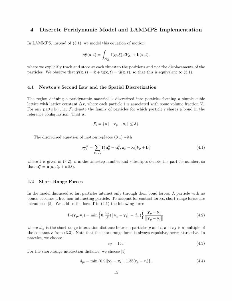
In LAMMPS, instead of (3.1), we model this equation of motion:
ρy(x, t) =∫Hx
f(η, ξ) dVx′ + b(x, t),
where we explicitly track and store at each timestep the positions and not the displacements of theparticles. We observe that y(x, t) = x + u(x, t) = u(x, t), so that this is equivalent to (3.1).
4.1 Newton’s Second Law and the Spatial Discretization
The region defining a peridynamic material is discretized into particles forming a simple cubiclattice with lattice constant ∆x, where each particle i is associated with some volume fraction Vi.For any particle i, let Fi denote the family of particles for which particle i shares a bond in thereference configuration. That is,
Fi = {p | ‖xp − xi‖ ≤ δ}.
The discretized equation of motion replaces (3.1) with
ρyni =
∑p∈Fi
f(unp − un
i ,xp − xi)Vp + bni (4.1)
where f is given in (3.2), n is the timestep number and subscripts denote the particle number, sothat un
i = u(xi, t0 + n∆t).
4.2 Short-Range Forces
In the model discussed so far, particles interact only through their bond forces. A particle with nobonds becomes a free non-interacting particle. To account for contact forces, short-range forces areintroduced [5]. We add to the force f in (4.1) the following force
fS(yp,yi) = min{
0,cS
δ(∥∥yp − yi
∥∥− dpi)} yp − yi∥∥yp − yi
∥∥ , (4.2)
where dpi is the short-range interaction distance between particles p and i, and cS is a multiple ofthe constant c from (3.3). Note that the short-range force is always repulsive, never attractive. Inpractice, we choose
cS = 15c. (4.3)
For the short-range interaction distance, we choose [5]
dpi = min {0.9 ‖xp − xi‖ , 1.35(rp + ri)} , (4.4)
15

where ri is called the node radius of particle i. Given a discrete lattice, we choose ri to be half thelattice constant.2 Given this definition of dpi, contact forces appear only when particles are undercompression.
When accounting for short-range forces, it is convenient to define the short-range family ofparticles
FSi = {p |
∥∥yp − yi
∥∥ ≤ dpi}.
4.3 Modification to the Particle Volume
In a situation where two particles share a bond with ‖xp − xi‖ = δ, for example, we suppose thatonly approximately half the volume of each particle is “seen” by the other [5]. When computingthe force of each particle on the other we use Vp/2 rather than Vp in (4.1). As such, we introduce anodal volume scaling function for all bonded particles where δ− ri ≤ ‖xp − xi‖ ≤ δ (c.f. Figure 1).
We choose to use a linear unitless nodal volume scaling function
ν(xp − xi) =
− 1
2ri‖xp − xi‖+
(δ
2ri+ 1
2
)if δ − ri ≤ ‖xp − xi‖ ≤ δ
1 if ‖xp − xi‖ ≤ δ − ri
0 otherwise
If ‖xp − xi‖ = δ, ν = 0.5, and if ‖xp − xi‖ = δ − ri, ν = 1.0, for example.
4.4 Discrete Equation of Motion
The semi-discrete equation of motion can be written as
ρyni = c
∑p∈Fi
(∥∥yp − yi
∥∥− ‖xp − xi‖‖xp − xi‖
)µ(t,η, ξ)ν(xp − xi)Vp
yp − yi∥∥yp − yi
∥∥+
∑p∈FS
i
min{
0,cS
δ(∥∥yp − yi
∥∥− dip)}
Vp
yp − yi∥∥yp − yi
∥∥ + bni ,
accounting for short-range forces and nodal volume scaling.
When discretizing time in LAMMPS, we instead use a velocity-Verlet scheme, where both theposition and velocity of the particle are stored explicitly. The velocity-Verlet scheme (Algorithm1) is generally expressed in three steps, as where m denotes the mass of a particle, and f
n
i is thenet force on particle i at timestep n.
2For a simple cubic lattice, ∆x = ∆y = ∆z.
16

(a) Two-dimensional diagram show-ing particle on mesh (solid lines) withhorizon δ as grey circular region. Dualmesh (dotted lines) shows boundariesof each particle.
y
1
2
3
x
4 5
(b) Plot of ν(xp − xi) vs. ‖xp − xi‖.
Figure 1. Diagram showing horizon of a particular particle,demonstrating that the volume associated with particles near theboundary of the horizon is not completely contained within thehorizon.
Algorithm 1 Velocity Verlet
1: vn+1/2i = vn
i + ∆t2m f
n
i
2: yn+1i = yn
i + ∆tvn+1/2i
3: vn+1i = vn+1/2
i + ∆t2m f
n+1
i
4.5 Breaking Bonds
During the course of simulation, it may be necessary to break bonds, as described in section 3.3.A naıve implementation would have us first loop over all bonds and compute smin in (3.5), thenloop over all bonds again and break bonds with a stretch s > s0 as in (3.4), and finally loop overall particles and compute forces for the next step of Algorithm 1. For reasons of computationalefficiency, we will utilize the values of s0 from the previous timestep when deciding to break abond. For the first timestep, s0 is initialized to ∞ for all nodes. This means that no bonds maybe broken until the second timestep. As such, it is recommended that the first few timesteps ofthe peridynamic simulation not involve any actions that might result in the breaking of bonds. Asa practical example, the projectile in the next section is placed such that it does not impact thebrittle plate until several timesteps into the simulation.
17

4.6 PseudoCode
A sketch of the peridynamic implementation in LAMMPS appears in Algorithm 2.
Algorithm 2 PMB Peridynamic Model in LAMMPS1: Fix s00, α, horizon δ, spring constant c, timestep ∆t, and generate initial lattice of particles with lattice constant
∆x. Let there be N particles.2: Initialize bonds between all particles where ‖x− x′‖ ≤ δ.3: Initialize s0 = ∞ {Initialize each entry to MAX DOUBLE.}4: while not done do5: Perform step 1 of Algorithm 1, updating velocities of all particles.6: Perform step 2 of Algorithm 1, updating positions of all particles.7: s0 = ∞ {Initialize each entry to MAX DOUBLE.}8: for i = 1 to N do9: {Compute short-range forces}
10: for all particles j ∈ FSi (the short-range family of nodes for particle i) do
11: r =∥∥yi − yj
∥∥.12: dr = min{0, r − d}. {Short-range forces are only repulsive, never attractive}13: k = cS
δVkdr. {cS defined in (4.3)}
14: f = f − kyi−yj
‖yi−yj‖.
15: end for16: end for17: for i = 1 to N do18: {Compute bond forces.}19: for all particles j sharing a bond with particle i do20: r =
∥∥yi − yj
∥∥.21: dr = r − ‖xi − xj‖.22: k = c
‖xi−xj‖Vjν(xi − xj)dr. {c defined in (3.3)}
23: f = f − kyi−yj
‖yi−yj‖.
24: if dr
‖xi−xj‖ > min(s0(i), s0(j)) then
25: Break i’s bond with j. {j’s bond with i will be broken when this loop iterates on j}26: end if27: s0(i) = min(s0(i), s00 − α dr
‖xi−xj‖ ).
28: end for29: end for30: s0 = s0. {Store for use in next timestep.}31: Perform step 3 of Algorithm 1, updating velocities of all particles.32: end while
4.7 Damage
The damage associated with every particle (see (3.6)) can optionally be computed and output witha LAMMPS data dump. To do this, your input script must contain the command
compute <ComputeID> all damage/atom
This enables a LAMMPS per-atom compute to calculate the damage associated with each particleevery time a LAMMPS data dump is called. To output the results of this compute in your dump
18

file, you must use the LAMMPS dump command, as
dump <DumpID> all custom <N> <output filename> tag type x y z c_<ComputeID>
where N is the number of timesteps between dumps.
4.8 Pitfalls
Parallel Scalability. LAMMPS operates in parallel in a spatial-decomposition mode [4], whereeach processor owns a spatial subdomain of the overall simulation domain and communicates withits neighboring processors via distributed-memory message passing (MPI) [7] to acquire ghost atominformation to allow forces on the atoms it owns to be computed. LAMMPS also uses Verlet neigh-bor lists which are recomputed every few timesteps as particles move. On these timesteps, particlesalso migrate to new processors as needed. LAMMPS decomposes the overall simulation domainso that spatial subdomains of nearly equal volume are assigned to each processor. When eachsubdomain contains nearly the same number of particles, this results in a reasonable load balanceamong all processors. As is more typical with some peridynamic simulations, some subdomains maycontain many particles while other subdomains contain few particles, resulting in a load imbalancethat impacts parallel scalability.
Setting the “skin” distance. The neighbor command with LAMMPS is used to set theso-called “skin” distance used when building neighbor lists. All atom pairs within a cutoff distanceequal to the horizon δ plus the skin distance are stored in the list. Unexpected crashes in LAMMPSmay be due to too small a skin distance. The skin should be set to a value such that δ plus the skindistance is larger than the maximum possible distance between two bonded particles. For example,if s00 is increased, the skin distance may also need to be increased.
“Lost” particles. All particles are contained within the “simulation box” of LAMMPS. Theboundaries of this box may change with time, or not, depending on how the LAMMPS boundarycommand has been set. If a particle drifts outside the simulation box during the course of asimulation, it is called lost.
As an option of the themo_modify command of LAMMPS, the lost keyword determines whetherLAMMPS checks for lost atoms each time it computes thermodynamics and what it does if atomsare lost. If the value is ignore, LAMMPS does not check for lost atoms. If the value is error orwarn, LAMMPS checks and either issues an error or warning. The code will exit with an error andcontinue with a warning. This can be a useful debugging option. The default behavior of LAMMPSis to exit with an error if a particle is lost.
The peridynamic module within LAMMPS does not check for lost atoms. If a particle withunbroken bonds is lost, those bonds are marked as broken by the remaining particles.
19
Defining the peridynamic horizon δ. In the pair_coeff command, the user must specify thehorizon δ. This argument determines which particles are bonded when the simulation is initialized.It is recommended that δ be set to a small fraction of a lattice constant larger than desired.
For example, if the lattice constant is 0.0005 and you wish to set the horizon to three timesthe lattice constant, then set δ to be 0.0015001, a value slightly larger than three times the latticeconstant. This guarantees that particles three lattice constants away from each other are stillbonded. If δ is set to 0.0015, for example, floating point error may result in some pairs of particlesthree lattice constants apart not being bonded.
4.9 Bugs
The user is cautioned that this code is a beta release. If you are confident that you have founda bug in the peridynamic module, please send an email to the developers. First, check the “Newfeatures and bug fixes” section of the LAMMPS website site to see if the bug has already beenreported or fixed. If not, the most useful thing you can do for us is to isolate the problem. Runit on the smallest number of atoms and fewest number of processors and with the simplest inputscript that reproduces the bug. In your email, describe the problem and any ideas you have as towhat is causing it or where in the code the problem might be. We’ll request your input script anddata files if necessary.
4.10 Modifying and Extending the Peridynamic Module
The peridynamic module of LAMMPS contains only a simple implementation of the PMB peri-dynamic model. To add new features or peridynamic potentials to the peridynamic module, theuser is referred to section 8 of the LAMMPS user manual, Modifying & extending LAMMPS. It issuggested that the user start with the PMB model as a template.
20

5 A Numerical Example
To introduce the peridynamic implementation within LAMMPS, we replicate a numerical experi-ment taken from section 6 of [6].
5.1 Problem Description and Setup
We consider the impact of a rigid sphere on a homogeneous disk of brittle material. The spherehas diameter 0.01 m and velocity 100 m/s directed normal to the surface of the target. The targetmaterial has density ρ = 2200 kg/m3. A PMB material model is used with k = 14.9 GPa andcritical bond stretch parameters given by s00 = 0.0005 and α = 0.25. A three-dimensional simplecubic lattice is constructed with lattice constant 0.0005 m and horizon 0.0015 m. (The horizonis three times the lattice constant.) The target is a cylinder of diameter 0.074 m and thickness0.0025 m, and the associated lattice contains 103,110 particles. Each particle i has volume fractionVi = 1.25× 10⁻¹⁰ m3.
The spring constant in the PMB material model is
c =18k
πδ4=
18(14.9× 10⁹)π(1.5× 10⁻³)4
≈ 1.6863× 10²². (5.1)
The CFL analysis from [6] shows that a timestep of 1.0× 10⁻⁷ is safe.
We observe here that in IEEE double-precision floating point arithmetic when computing thebond stretch s(t, η, ξ) at each iteration where ‖η + ξ‖ is computed during the iteration and ‖ξ‖was computed and stored for the initial lattice, it may be that fl(s) = ε with |ε| ≤ εmachine for anunstretched bond. Taking ε = 2.220446049250313×10⁻¹⁶, we see that the value csVi ≈ 4.68×10⁻⁴,computed when determining f , is perhaps larger than we would like, especially when the true forceshould be zero. One simple way to avoid this issue is to insert the following instructions in Algorithm2 after instruction 21:1: if |dr| < εmachine then2: dr = 0.3: end if
Qualitatively, this says that displacements from equilibrium on the order of 10−6A are taken to beexactly zero, a seemingly reasonable assumption.
5.2 The Projectile
The projectile used in the following experiments is not the one used in [6]. The projectile used hereexerts a force
F (r) = −ks(r −R)2
on each atom where ks is a specified force constant, r is the distance from the atom to the center ofthe indenter, and R is the radius of the projectile. The force is repulsive and F (r) = 0 for r > R.
21

For our problem, the projectile radius R = 0.05 m, and we have chosen ks = 1.0 × 10¹⁷ (comparewith (5.1) above).
5.3 Writing the LAMMPS Input File
We discuss the example input script from Algorithm 3. In line 2 we specify that SI units areto be used. We specify the dimension (3) and boundary conditions (“shrink-wrapped”) for thecomputational domain in lines 3 and 4. In line 5 we specify that peridynamic particles are tobe used for this simulation. In line 7, we set the “skin” distance used in building the LAMMPSneighborlist. In line 8 we set the lattice constant (in meters) and in line 10 we define the spatialregion where the target will be placed. In line 12 we specify a rectangular box enclosing the targetregion that defines the simulation domain. Line 14 fills the target region with atoms. Lines 15and 17 define the peridynamic pairwise force function, and lines 19 and 21 set the particle densityand particle volume, respectively. The particle volume should be set to the cube of the latticeconstant for a simple cubic lattice. Line 23 sets the initial velocity of all particles to zero. Line25 instructs LAMMPS to integrate time with velocity-Verlet, and line 27 creates the sphericalprojectile, sending it with a velocity of 100 m/s towards the target. Line 29 declares a computestyle for the damage (percentage of broken bonds) associated with each particle. Line 30 sets thetimestep, line 31 instructs LAMMPS to provide a screen dump of thermodynamic quantities every200 timesteps, and line 32 instructs LAMMPS to create a data file (dump.output) with a completesnapshot of the system every 100 timesteps. This file can be used to create still images or movies.Finally, line 33 instructs LAMMPS to run for 2,000 timesteps.
5.4 Numerical Results and Discussion
We ran the input script from Algorithm 3. Images of the disk (projectile not shown) appear inFigure 2. Visualization was done with the EnSight visualization package [1]. The LAMMPS dumpfile was converted to an EnSight format with the pizza.py toolkit [3]. The plot of damage on thetop monolayer was created by coloring each particle according to its damage (see (3.6)).
The symmetry in the computed solution arises because a “perfect” lattice was used, and abecause a perfectly spherical projectile impacted the lattice at its geometric center. To break thesymmetry in the solution, the nodes in the peridynamic body must be perturbed slightly from thelattice sites. To do this, a perturbed lattice of points can be prepared in a data file and read intoLAMMPS using the read_data command.
22

Algorithm 3 Example LAMMPS Input Script1: # 3D Peridynamic simulation with projectile
2: units si
3: dimension 3
4: boundary s s s
5: atom_style peri
6: atom_modify map array
7: neighbor 0.0010 bin
8: lattice sc 0.0005
9: # Create desired target
10: region target cylinder y 0.0 0.0 0.037 -0.0025 0.0 units box
11: # Make 1 atom type
12: create_box 1 target
13: # Create the atoms in the simulation region
14: create_atoms 1 region target
15: pair_style peri/pmb
16: # <type1> <type2> <c> <horizon> <s00> <alpha>
17: pair_coeff * * 1.6863e22 0.0015001 0.0005 0.25
18: # Set mass density
19: set group all density 2200
20: # volume = lattice constant^3
21: set group all volume 1.25e-10
22: # Zero out velocities of particles
23: velocity all set 0.0 0.0 0.0 sum no units box
24: # Use velocity-Verlet time integrator
25: fix F1 all nve
26: # Construct spherical indenter to shatter target
27: fix F2 all indent 1e17 sphere 0.0 0.0051 0.0 0.005 vel 0.0 -100.0 0.0 units box
28: # Compute damage for each particle
29: compute C1 all damage/atom
30: timestep 1.0e-7
31: thermo 200
32: dump D1 all custom 100 dump.output tag type x y z c_C1
33: run 2000
23

(a) Cut view of target during impact.
(b) Top monolayer showing fragmenta-tion.
(c) Top monolayer showing damage. (blue= 0% broken bonds; red = 100% brokenbonds)
Figure 2. Target during (a) and after (b,c) impact.
24

References
[1] CEI, EnSight web page. http://www.ensight.com/.
[2] E. Emmrich and O. Weckner, On the well-posedness of the linear peridynamic model andits convergence towards the Navier equation of linear elasticity, Commun. Math. Sci., 5 (2007),pp. 851–864.
[3] S. J. Plimpton, Pizza.py webpage. http://www.cs.sandia.gov/~sjplimp/pizza.html.
[4] S. J. Plimtpon, Fast parallel algorithms for short-range molecular dynamics, J. Comp. Phys.,117 (1995), pp. 1–19. Available at http://lammps.sandia.gov.
[5] S. A. Silling. Personal communication, 2007.
[6] S. A. Silling and E. Askari, A meshfree method based on the peridynamic model of solidmechanics, Computer and Structures, 83 (2005), pp. 1526–1535.
[7] M. Snir, S. Otto, S. Huss-Lederman, D. Walker, and J. Dongarra, MPI: The Com-plete Reference, vol. 1, The MIT Press, Cambridge, MA., 2 ed., 1998.
25
DISTRIBUTION:
1 MS 1322 John Aidun, 1435
1 MS 1318 Ken Alvin, 1416
1 MS 1320 Scott Collis, 1414
1 MS 1320 Richard Lehoucq, 1414
1 MS 1320 Michael Parks, 1414
1 MS 1316 Steven Plimpton, 1416
1 MS 1322 Stewart Silling, 1435
1 MS 0899 Technical Library, 9536 (electronic copy)
1 MS 0123 D. Chavez, LDRD Office, 1011
26

v1.27
