Performance of the new small-strip Thin Gap Chamber for the

ATLAS Muon System at the LHC Alain Bellerive

Canada Research Professor Carleton University, Ottawa, Canada

Outline

§  Introduction –  Motivation –  ATLAS at the LHC

§  The New Small Wheel (NSW) §  The small-strip Thin Gap Chambers (sTGC)

–  Design of the sTGC –  Performance & Characterization –  Digitization Model

§  Summary and Conclusion

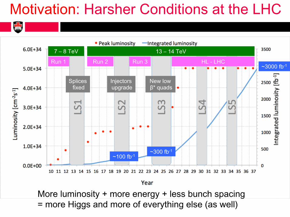
Motivation: Harsher Conditions at the LHC

7 – 8 TeV 13 – 14 TeV

Run 1 Run 2 Run 3 HL - LHC

~100 fb-1 ~300 fb-1

~3000 fb-1

Splices fixed

Injectors upgrade

New low β* quads

More luminosity + more energy + less bunch spacing = more Higgs and more of everything else (as well)

Collecting the data for new discoveries

§  Collision rate in ATLAS is huge – originally 25 every 50 ns

§  In future will be 50-100 every 25 ns

§  Need to select rare events with discovery potential

§  This is done by the “trigger” §  Key trigger selection looks for

energetic muons §  ATLAS trigger designed for

nominal LHC luminosity §  LHC luminosity of 3 – 6 times

the original design. §  To collect interesting events

we need to enhance ATLAS trigger capability

Early ATLAS running

Event from 2012 run

Collisions in one event in ATLAS

The ATLAS Detector

New Small Wheel

6000 tons 100 m underground

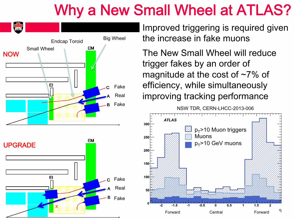
Why a New Small Wheel at ATLAS?

!"#$%#!$&!' (#')*+*,-.-' /'

Phase-1 : New small wheel

Kill the fake trigger by requiring high quality IP pointing segments in EI (small wheel) Precision tracker that works up to the ultimate luminosity, 5-7x1034 , with some safety margin

Small Wheel Endcap Toroid Big Wheel

X

Figure 2.6: ⇥ distribution of Level-1 muon signal (pT > 10GeV) (L1_MU11) with the distribution ofthe subset with matched muon candidate (within �R < 0.2) to an o�ine well reconstructedmuon (combined inner detector and muon spectrometer track with pT > 3GeV), and o�inereconstructed muons with pT > 10GeV.

• Measure the second coordinate with a resolution of 1–2mm to facilitate good linking betweenthe MS and the ID track for the combined muon reconstruction..

The background environment in which the NSW will be operating will cause the rejection ofmany hits as spurious, as they might have been caused by �-rays, neutron or other backgroundparticles. Furthermore in the life-time of the detector, detection planes may fail to operate properly,with very limited opportunities for repairing them. Hence a multi-plane detector is required.

Any new detector that might be installed in the place of the current Small Wheel should beoperational for the full life time of ATLAS (and be able to integrate 3000 fb�1). Assuming al least10 years of operation and the above expected hit rate per second, approximately 1012 hits/cm2 areexpected in total in the hottest region of the detector.

2.3 Trigger selection

Performance studies using collision data have shown the presence of unexpectedly high rates offake triggers in the end-cap region. Figure 2.6 shows the ⇥ distribution of candidates selected bythe ATLAS Level-1 trigger as muons with at least 10GeV. The distribution of those candidatesthat indeed have an o⇥ine reconstructed muon track is also shown, together with the muonsreconstructed with pT > 10GeV. More than 80% of the muon trigger rate is from the end-caps(|⇥| > 1.0), and most of the triggered objects are not reconstructible o⇥ine.

Trigger simulations show that selecting muons with pT > 20GeV at Level-1 (L1_MU20) onewould get a trigger rate at

⇥s=14 TeV and at an instantaneous luminosity of 3� 1034cm�2s�1 of

approximately 60 kHz, to be compared to the total available Level-1 rate of 100 kHz.In order to estimate the e�ect of a trigger using the NSW a study has been performed applying

o⇥ine cuts to the current SW to reduce the trigger rate. Table 2.1 shows the relative rate ofL1_MU20 triggers in the |⇥| > 1.3 region after successive o⇥ine cuts to select high quality muontracks. The various successive cuts applied are: i) the presence of Small Wheel track segments

21

pT>10 Muon triggers Muons pT>10 GeV muons

Forward Forward Central

NSW TDR, CERN-LHCC-2013-006

Improved triggering is required given the increase in fake muons

The New Small Wheel will reduce trigger fakes by an order of magnitude at the cost of ~7% of efficiency, while simultaneously improving tracking performance

NOW

UPGRADE

Fake

Fake

Fake

Fake

Real

Real

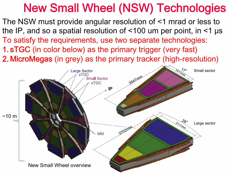
New Small Wheel (NSW) Technologies The NSW must provide angular resolution of <1 mrad or less to the IP, and so a spatial resolution of <100 um per point, in <1 μs To satisfy the requirements, use two separate technologies: 1.  sTGC (in color below) as the primary trigger (very fast) 2. MicroMegas (in grey) as the primary tracker (high-resolution)

Small sector

Large sector ~10 m

New Small Wheel overview

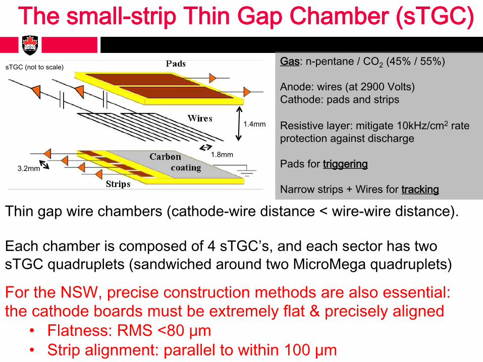
The small-strip Thin Gap Chamber (sTGC)

How a Thin Gap Chamber (TGC) Works

November 30, 2012 I. Trigger - ATLAS NSW Intro and Requirements 4

MWPC with !(anode-cathode) < !(anode-anode) i.e. gas-gap thickness < wire spacing

Single avalanche / limited streamer mode: thinness limits shower size and lateral extension

Resistive cathode coating stops photons propagating along wires; self-quenching gas (55% CO2 45% n-pentane) absorbs its own photons well

Wires ganged, precision coordinate is from Strips (3.2 mm pitch), Pads give local RoI

Thin gap wire chambers (cathode-wire distance < wire-wire distance). Each chamber is composed of 4 sTGC’s, and each sector has two sTGC quadruplets (sandwiched around two MicroMega quadruplets)

For the NSW, precise construction methods are also essential: the cathode boards must be extremely flat & precisely aligned •  Flatness: RMS <80 μm •  Strip alignment: parallel to within 100 μm

Gas: n-pentane / CO2 (45% / 55%) Anode: wires (at 2900 Volts) Cathode: pads and strips Resistive layer: mitigate 10kHz/cm2 rate protection against discharge Pads for triggering Narrow strips + Wires for tracking

1.4mm

3.2mm

1.8mm

sTGC (not to scale)

Testbeam at Fermilab (FNAL)

FNAL Experimental Setup sTGC

Remote control motion table Scan sTGC with pixel telescope (σ≈4μm) •  allow independent measurement of s-shape bias correction and gap alignment •  residual analysis for determination of single hit strip resolution •  study trigger pad efficiency

pixel telescope

sTGC

motion table

beam

strips (along x) cluster to

measure y(hit)

r Δθ ≈ Δy = σ = y(sTGC) – y(pixel)

pad

wire

strip

Amplitude on ith strip

Hit position

Position of center of ith strip

Strip response width

Knowing the reference track with the pixel detector allowed to determine, without assumption, the shape of the “strip” response function

sTGC: hit reconstruction

Distribution of charge

wire

strip

y(sTGC) ≈ rIP Δθ(ATLAS)

Determination of bias

True position (reference pixel)

Rec

onst

ruct

ed p

ositi

on (s

TGC

)

Determination of the track position: •  Pixel detector allowed extrapolation of the position of the hit with a 4 microns precision •  Bias correction parameterized as a sine wave

Intrinsic sTGC bias due to: •  Collection of charge not continuous since the strips are discrete •  Distribution of charge NOT Gaussian

Hit position sTGC – Hit position pixel detector

Single-hit strip spatial resolution: 45 ± 8 μm

σ = 45 ± 8 μm All runs – All layers

NIM, Volume 817, 1 May 2016, p.85–92

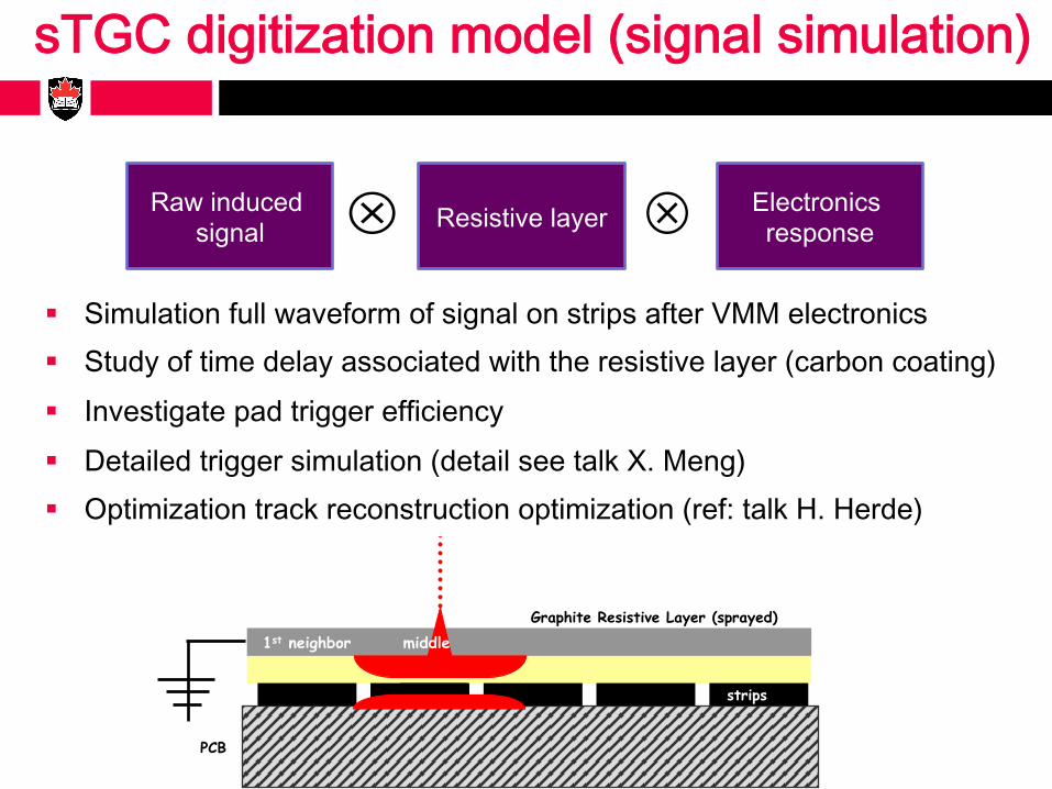
Raw induced signal ⊗ Resistive layer ⊗ Electronics

response

Graphite Resistive Layer (sprayed)

strips

PCB

1st neighbor middle

sTGC digitization model (signal simulation)

§  Simulation full waveform of signal on strips after VMM electronics §  Study of time delay associated with the resistive layer (carbon coating) §  Investigate pad trigger efficiency §  Detailed trigger simulation (detail see talk X. Meng) §  Optimization track reconstruction optimization (ref: talk H. Herde)

Graphite Resistive Layer (sprayed)

strips

PCB

1st neighbor middle

sTGC digitization model (signal simulation)

0 0.2 0.4 0.6 0.8 1

0

10000

20000

30000

40000

50000

Shaped Charge vs Time Strip 3Shaped Charge vs Time Strip 3

0 0.2 0.4 0.6 0.8 1

0

1000

2000

3000

4000

5000

6000

7000

8000

Shaped Charge vs Time Strip 4Shaped Charge vs Time Strip 4

0 0.2 0.4 0.6 0.8 10

200

400

600

800

1000

1200

1400

1600

Shaped Charge vs Time Strip 5Shaped Charge vs Time Strip 5

1000 ns

Strip main (middle) Strip (1st neighbor) Strip 2nd neighbor

1000 ns 1000 ns

1st neighbor 2nd neighbor 3rd neighbor

Amplitude versus time Amplitude versus time Amplitude versus time

Summary and Conclusion

§  LHC upgrades provide the opportunity to really improve our knowledge of the Higgs boson, the Standard Model and the search for new physics

§  However, in its current state ATLAS would be unable to take advantage of these opportunities.

§  Upgrade work for construction and installation of the New Small Wheel (NSW) during the next shutdown (LS2) is ongoing

§  The first full scale sTGC module meets the specification with single-hit spatial resolution (σ = 45 ± 8 μm)

§  sTGC digitization simulation for detailed trigger simulation and track reconstruction optimization

§  ATLAS Canada is in the middle of a number of important efforts for the future of ATLAS

Extra…

Physics at the Large Hadron Collider (LHC)

§  Physics at the LHC: study of the Higgs boson and of the Standard Model, investigate of rare processes, search for new physics like super-symmetry and dark matter

§  All these processes are very rare and require lots of energy, so many high-energy collisions will be needed to make precision measurements.

§  The energy and number of collisions at the LHC are largely determined by three parameters: –  Center-of-mass energy –  Bunch spacing: accelerators are pulsed, with particles arriving in

bunches, rather than continuously. The bunch spacing is the time between two bunches

–  (Instantaneous) Luminosity: essentially measures the rate at which the accelerator produces collisions (collisions/area/time)

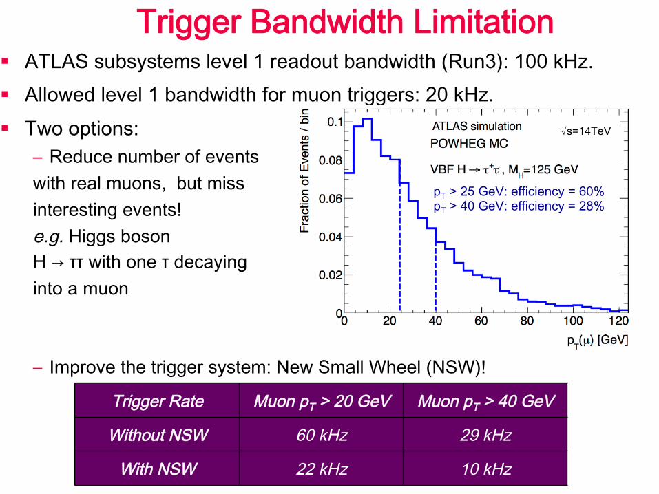
§  ATLAS subsystems level 1 readout bandwidth (Run3): 100 kHz. §  Allowed level 1 bandwidth for muon triggers: 20 kHz. §  Two options:

–  Reduce number of events with real muons, but miss interesting events! e.g. Higgs boson H → ττ with one τ decaying into a muon

–  Improve the trigger system: New Small Wheel (NSW)!

Trigger Bandwidth Limitation

Trigger Rate Muon pT > 20 GeV Muon pT > 40 GeV

Without NSW 60 kHz 29 kHz

With NSW 22 kHz 10 kHz

pT > 25 GeV: efficiency = 60% pT > 40 GeV: efficiency = 28%

√s=14TeV