A1 1

SUMMARY 1. Global Behavior of the Containment Vessel LST (Model 3)

2. Modeling of the initial state

3. Permeability of the Containment Vessel

4. Rupture of linear seal (Model 2)

Veronique LE CORVEC

Mahsa MOZAYAN KHARAZI

Charles GHAVAMIAN

PERFORMANCE OF CONTAINMENT VESSEL UNDER SEVERE ACCIDENT CONDITIONS

SPE analysis meeting #3 March 27-29, 2012, Washington DC

Sylvie MICHEL-PONNELLE

Etienne GALLITRE

A1 2

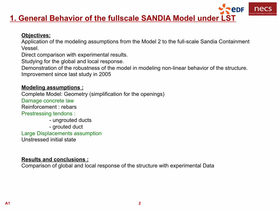
Objectives: Application of the modeling assumptions from the Model 2 to the full-scale Sandia Containment Vessel. Direct comparison with experimental results. Studying for the global and local response. Demonstration of the robustness of the model in modeling non-linear behavior of the structure. Improvement since last study in 2005 Modeling assumptions : Complete Model: Geometry (simplification for the openings) Damage concrete law Reinforcement : rebars Prestressing tendons :

- ungrouted ducts - grouted duct

Large Displacements assumption Unstressed initial state Results and conclusions : Comparison of global and local response of the structure with experimental Data

1. General Behavior of the fullscale SANDIA Model under LST

A1 3

Model geometry

Internal radius = 5.7 m

External radius = 5.375 m

Total Height= 22.5 cm

Number of Elements: ~ 18 000 Number of Elements in the wall thickness: ~ 3/5 elements Finer mesh for the Openings: -  E/H Hatch -  A/L Hatch

A1 4

Components of the model :

Component Element type Material model

Concrete Structure 3D brick element

Vessel, Dome Concrete Damage law

Foundations, Buttress Linear Elastic Material

Liner 2D plate element (DKT) Plastic Material ( VMIS)

Reinforcement bars 2D membrane element

Prestressing tendons 1D elements Associated with 1D string element

Linear Elastic Material

!

!

A1 5

Concrete constitutive model MAZARS -> ENDO-ISOT Features : -  Based on damage mechanics -  Limit in traction (tension / compression distinction) -  Linear response in compression -  Isotropic damage effect (single scalar damage index D) -  Crack reclosure

Tension

S

tress

(MP

a)

Compression

klijklij CD εσ )1( −=

Strain

S

tress

(MP

a)

Strain

Parameter: SYT = 2.4E6 , D_SIGM_EPSI = -1.0e9

A1 6

!

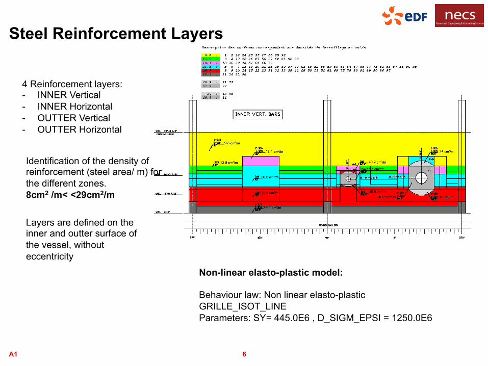
4 Reinforcement layers: -  INNER Vertical -  INNER Horizontal -  OUTTER Vertical -  OUTTER Horizontal

Steel Reinforcement Layers

Identification of the density of reinforcement (steel area/ m) for the different zones. 8cm2 /m< <29cm2/m

Layers are defined on the inner and outter surface of the vessel, without eccentricity

Non-linear elasto-plastic model: Behaviour law: Non linear elasto-plastic GRILLE_ISOT_LINE Parameters: SY= 445.0E6 , D_SIGM_EPSI = 1250.0E6

A1 7

Prestressing Tendons

Modeling of the complete set of ~180 cables With finer mesh

A1 8

Tendons section = 3.393 cm² (each tendon)

Tendon steel constitutive model Elastoplastic Parameters: Young Modulus in elastic phase (E) = 191 000 MPa

Young Modulus in plastic phase (E) = 5 894 MPa

Poisson's ratio (ν) = 0.3

Density (ρ) = 7850 kg/m3

Yield Strength (Ys) = 1 679MPa

Tensile Strength (XXX) = 1 856.76 MPa

Density (ρ) = 7850 kg/m3

Angular and wobble friction: µ =0.21; λ = 0.001

Prestressing Loading: - Initial Prestressing Force Hoop Tendons = 43.21t

Vertical Tendons =48.02 t -  Setting Losses Hoop Tendons = 0.00395

Vertical Tendons = 0.005

Tendon’s  node θ

z

r Concrete’s  node

(perfectly bonded in Z and R direction, friction along tendon direction)

Coefficient for bonding kx,ky,kz =1e9

Ungrouted Model

A1 9

Results

-  Global structural Behavior: deformed shape Comparison radial and vertical displacement with experimental results

-  Damage evolution in the Vessel

-  Evolution of the axial force in the prestressing tendons

-  Response of the Liner

A1 10

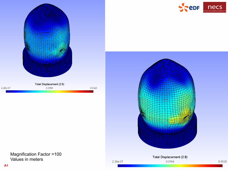
Magnification Factor =100 Values in meters

A1 11

‘Discontinuity in deformed shape’

Magnification Factor =100 Values in meters

A1 12

Radial Displacements

Z=0.25m Z=1.43m Z=2.63m

Z=6.2m Z=9.23m Z=14.55m

A1 13

Vertical Displacements

Z=2.63m Z=4.68m

Z=7.73m Z=12.8m Z=14.55m

A1 14

SOL #8 - Vertical Displacement

-5,00

5,00

15,00

0,00

0,39

0,79 1,1

8

1,57

Pressure (MPa)

Disp

lace

ment

(mm

)

LST-Data-of-Record

LST-Dynamic

SFMT

NNC ABAQUS V6.4

NNC ANAMAT

EGP

GRS

IRSN-CEA

KAERI-AXISYM

KAERI 3D

KOPEC

NRC-SNL-DEA

SCANSCOT

EDF

!

A1 15

Effect of small displacements/ versus Updated geometry

A1 16

!!

Deformed shape with updated geometry P = 3.6 x pd= 1.40 MPa - Magnification factor: 5

Deformed shape with small displacement assumption

A1 17

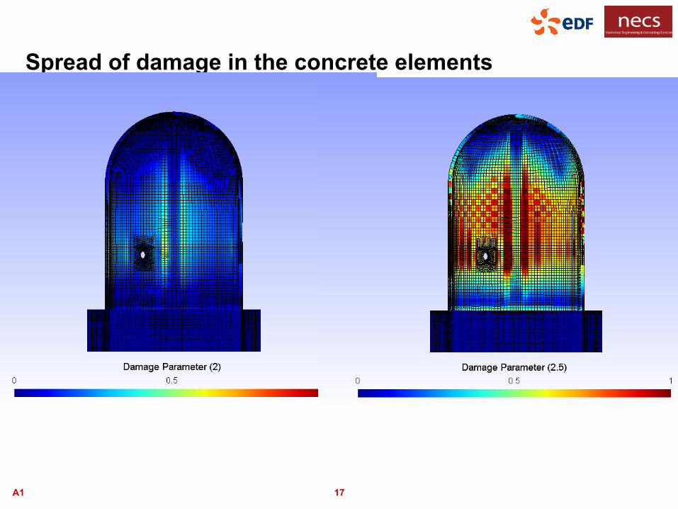
Spread of damage in the concrete elements

A1 18

P =3.2Pd

A1 19

Liner Response

A1 20

A1 21

Tendons Response

Grouted tendon

Ungrouted tendon (plain line)

(dotted line)

A1 22

Grouted tendon

Ungrouted tendon (plain line)

(dotted line)

A1 23 Grouted tendon

Ungrouted tendon (plain line)

(dotted line)

A1 24

Conclusions: -  Good estimation of the global behavior of the structure.

-  Better estimation in the central Vessel ( far from foundations and dome)

-  Negligible Effect on the tendons modeling on the global response

-  Noteworthy effect of the choice of updated geometry for the calculation ( updated geometry ‘PETIT REAC’)

-  Comparison of the Grouted or Ungrouted cable modeling:

smoothening of the response (axial force) close to the openings.

A1 25

2. Initial State

Objective : How to model / account for the different lifts and its effects on the structural response of the structure ( short term / long term ) Modeling : Full-scale structure at three successive construction state Reinforcement rebars and tendons not accounted for in the model Concrete behavior Modeling -  Thermal effects: εT° : cooling of the concrete (ΔT = 40°C) -  Autogeneous effects : ε autogeneous° : according to EC2 -  Creep effects: ε creep° : according to EC2

A1 26

Model Assumption

Modeling : Full-scale structure at three successive construction state

3d brick elements , quadratic mesh for mechanical part Reinforcement rebars and tendons not accounted for in the model

C1 and C2

Foundations

C1 - C2

C3 - C4

Time = -6 months

Time = 0

Time = 2 months

Time = 4 months D1 – D2- D3

A1 27

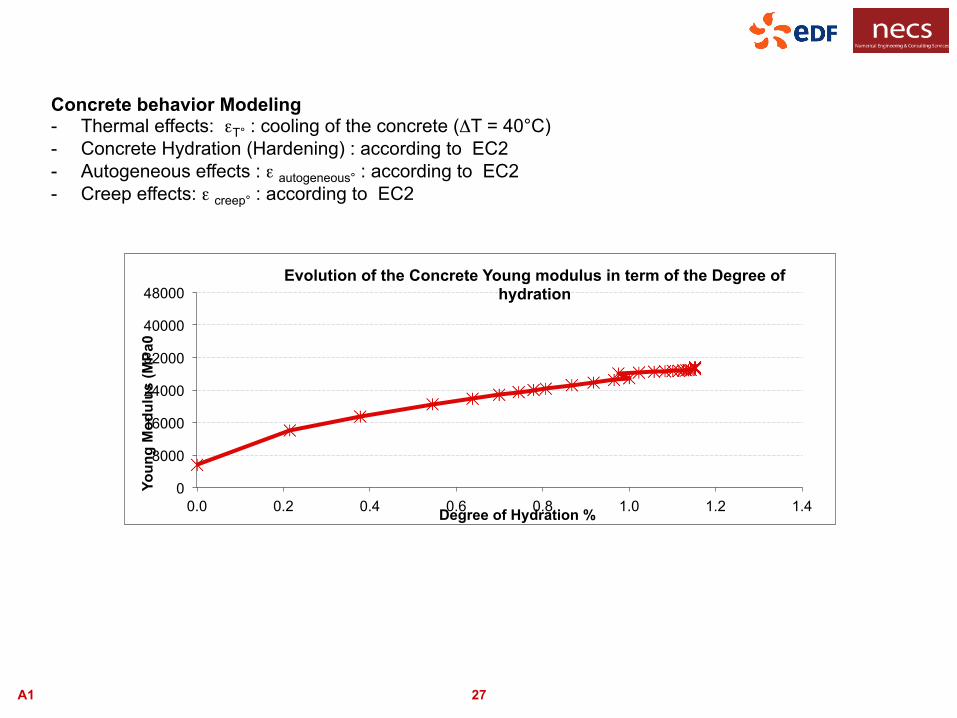
Concrete behavior Modeling -  Thermal effects: εT° : cooling of the concrete (ΔT = 40°C) -  Concrete Hydration (Hardening) : according to EC2 -  Autogeneous effects : ε autogeneous° : according to EC2 -  Creep effects: ε creep° : according to EC2

0

8000

16000

24000

32000

40000

48000

0.0 0.2 0.4 0.6 0.8 1.0 1.2 1.4

Youn

g M

odul

us (M

Pa0

Degree of Hydration %

Evolution of the Concrete Young modulus in term of the Degree of hydration

A1 28

Concrete behavior Modeling -  Thermal effects: εT° : cooling of the concrete (ΔT = 40°C) -  Concrete Hydration (Hardening) : according to EC2 -  Autogeneous effects : ε autogeneous° : according to EC2 -  Creep effects: ε creep° : according to EC2

Code_Aster:

Creep Law of Granger: Eurocode

Numerical Response

A1 29

Calculation process

Thermic Computation

Drying Computation

Mechanical Computation

Variation of T (time) Variation of xxx (time) Activation of the various effects (time) At each stage : thermic, hydratation, … At each lift : Activation of the new group element Accounting by the imposed displacement Of the part already constructed Activation of all the proprieties after setting of the concrete

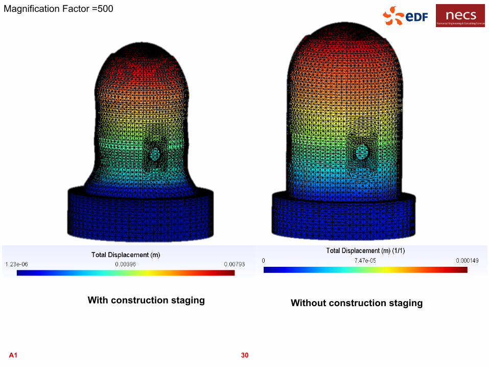
A1 30

Magnification Factor =500

With construction staging Without construction staging

A1 31

A1 32

Stress Profiles at 6 months (Inner surface)

A1 33

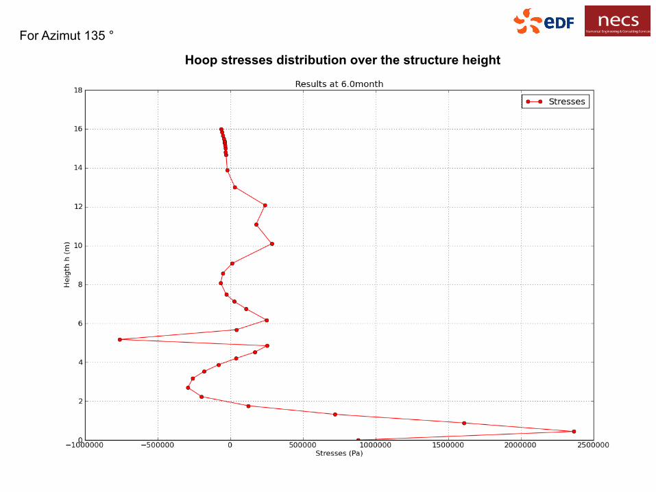
For Azimut 135 °

Hoop stresses distribution over the structure height

A1 34

Autogeneous Strain

Mechanical Strain

Thermal Strain

Total Strain

Hoop strains decomposition over the structure height

A1 35

-  Interest of studying the different effects intervening in the setting of concrete: creep, hydratation, young age -  Stresses map at initial state different from the unstressed initial state assumption

-  Future interest in more precise modeling of the phasing construction: drying effects w/wo with creep effects. account for the progressive prestressing of the cables use as initial state for LST test

Conclusions

A1 36

3. Permeability of the concrete wall

Objectives : Estimation of the permeability state of the wall Comparison between different configurations :

- initial state (permeability of concrete) - initial state with staging and aging effects (permeability of the concrete damaged)

Modeling : Complete structures No modeling of the cables Results : Map of gas flow for a given pressure and comparison between different configurations

A1 37

Hydraulic Equation

))()(()1( ggPg

l PgradPdivtP

S λφ −−=∂

∂−

gg

ggP P

KP

ηλ =)(

)1()1()( 25.4lllrg SSSK −−=

)()( DKSKKg lrg ×=Permeability

•  Relative permeability induced by degree of saturation

Permeability in term of Degree of saturation

Damage

Permeability

Saturation With Sl liquid water degree of Saturation Kg the gas permeability

A1 38

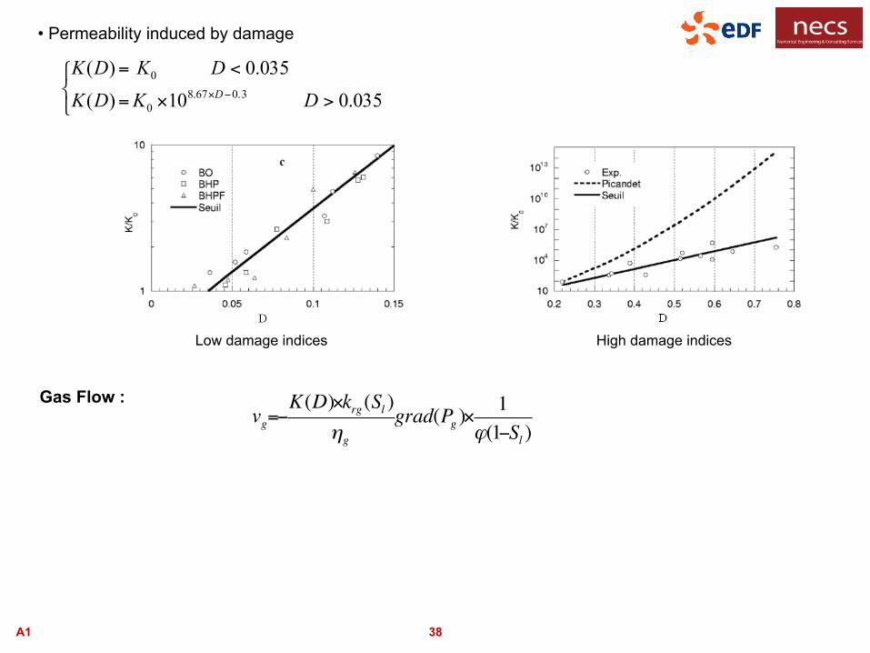
vg=!K(D)"krg(Sl )

!g

grad(Pg )"1

"(1!Sl )

•  Permeability induced by damage

⎩⎨⎧

>×=

<=−× 035.010)(

035.0)(3.067.8

0

0

DKDKDKDKD

Low damage indices High damage indices

Gas Flow :

A1 39 39/ 31

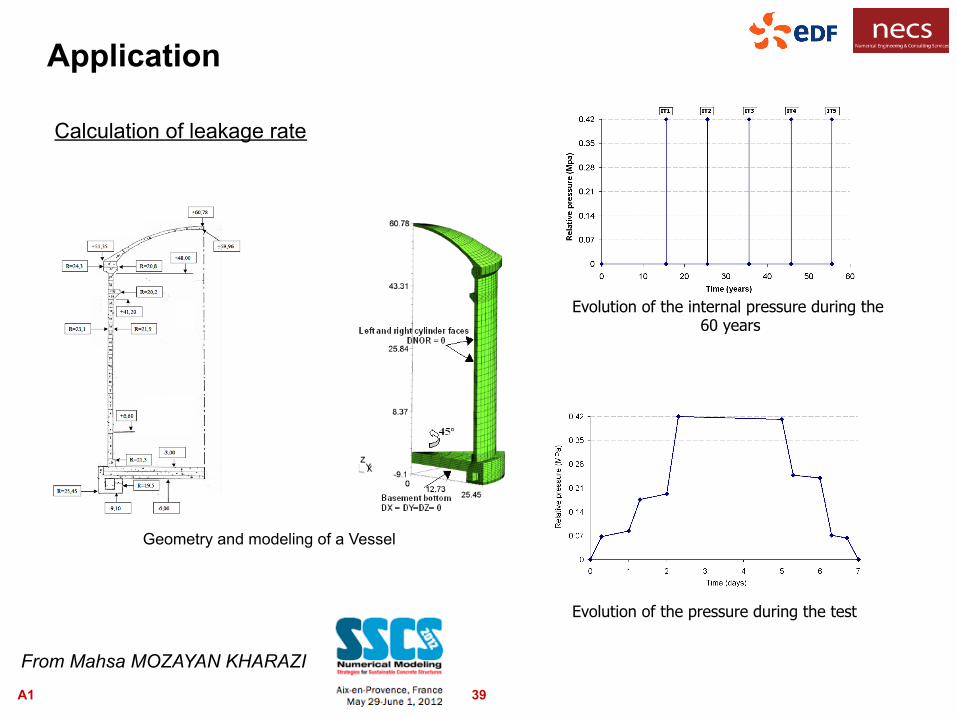
Application

Calculation of leakage rate

Evolution of the internal pressure during the 60 years

Evolution of the pressure during the test

Geometry and modeling of a Vessel

From Mahsa MOZAYAN KHARAZI

A1 40

Evolution of the Damage indice at each test Hydric Calculation:

Degree of saturation in the wall thickness for each test

Mechanical Calculation:

From Mahsa MOZAYAN KHARAZI

A1 41

Incoming massic gaz flow during tests Outgoing massic gaz flow during the tests (effect of the increasing damage)

Hydraulic Calculation :

From Mahsa MOZAYAN KHARAZI

A1 42

Application to the case of SANDIA: qualitative results

u  the deformations obtained with the model with staging after 1 year

Estimation of the local damage using Mazars Law

u  Saturation Hypothesis: Degree of Saturation :80%

A1 43

Leakage Map of the inner surface at a given pressure

A1 44

Conclusions

•  Development of a uncoupled thermo-hydro-mechanical methodology to compute leakage rate for containment without liner •  The method allows for measuring the effect of the degree of saturation and progressive damage

•  Limitations of the model for law damage structures. Improvement required for large cracks.

A1 45

4. Rupture of the Liner

Objective : Model the rupture of the liner with Cohesive Zone Model elements Modeling : Sub-structuration : - Extraction of the displacement field on the liner from the complete

structural model. - Application of the resulting displacements on certain zones of the liner.

- Study of the Liner response with 3 possible tears.

A1 46

Comparison Liner Hoop strains Experimental versus Numerical close to the E/H at the elevation 4.8m

A1 47

Liner hoop stresses close the E/H hatch at an elevation 4.8m

A1 48

Meshing: liner Solid element

Quadratic

Thickness 1.6mm

Liner perfectly bonded with concrete at nodes except around seal lines

Properties: same as for model 1

A1 49

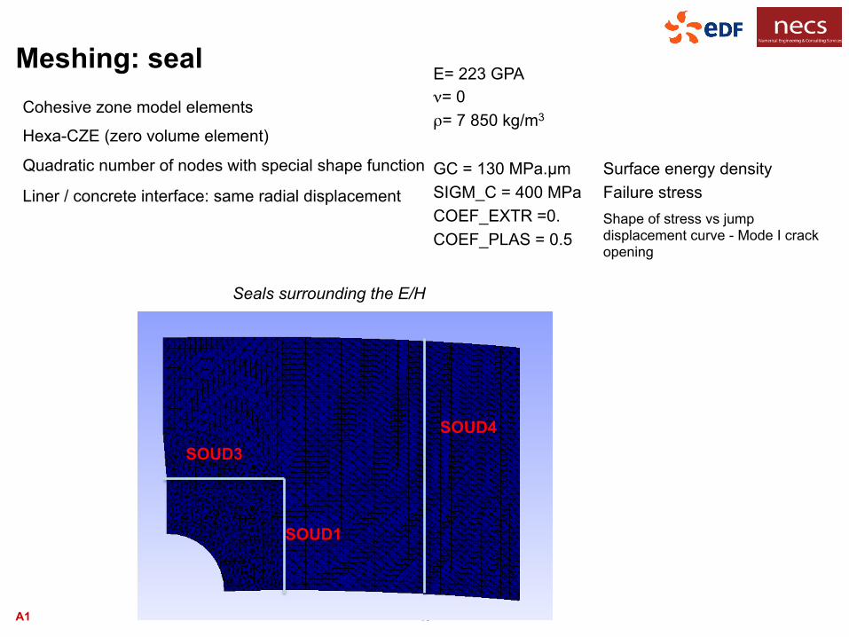
Meshing: seal Cohesive zone model elements

Hexa-CZE (zero volume element)

Quadratic number of nodes with special shape function

Liner / concrete interface: same radial displacement

Seals surrounding the E/H

E= 223 GPA ν= 0 ρ= 7 850 kg/m3 GC = 130 MPa.µm Surface energy density SIGM_C = 400 MPa Failure stress COEF_EXTR =0. COEF_PLAS = 0.5

Shape of stress vs jump displacement curve - Mode I crack opening

SOUD4

SOUD1

SOUD3

A1 50

Assembly of a cohesive element with adjacent liner elements

Cohesive zone model elements Example of tetra-cohesive zone elements with opening in Mode I

The cohesive law for ductile fracture

cσnσ

nδcδpδeδ

cG

2= + −c c c e pGδ σ δ δ e p cδ δ δ≤ <

( )

if

1 if

if

0 if

≤

< <=

−≤ <

−

≥

nn e

e

e n pn n c

c np n c

c p

n c

δδ δ

δ

δ δ δσ δ σ

δ δδ δ δ

δ δ

δ δ

A1 51

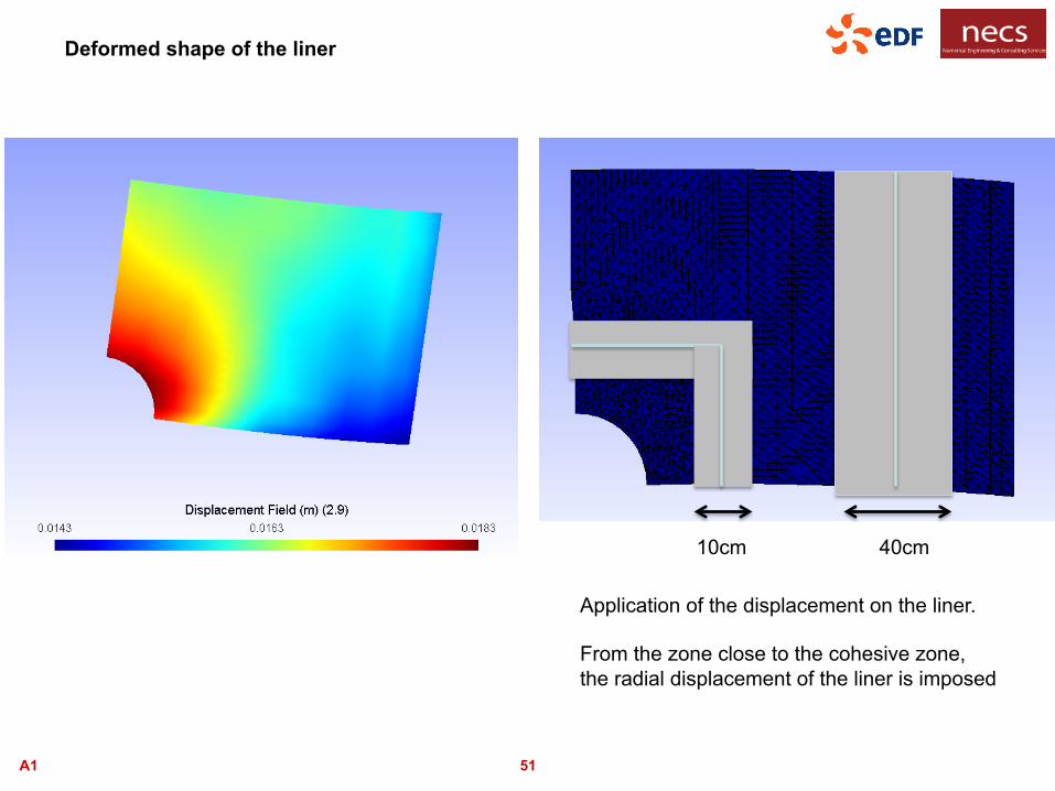
Deformed shape of the liner

Application of the displacement on the liner. From the zone close to the cohesive zone, the radial displacement of the liner is imposed

40cm 10cm

A1 52

Magnification Factor =10

Visualization of the opening of the seals at P=2.9Pd

A1 53

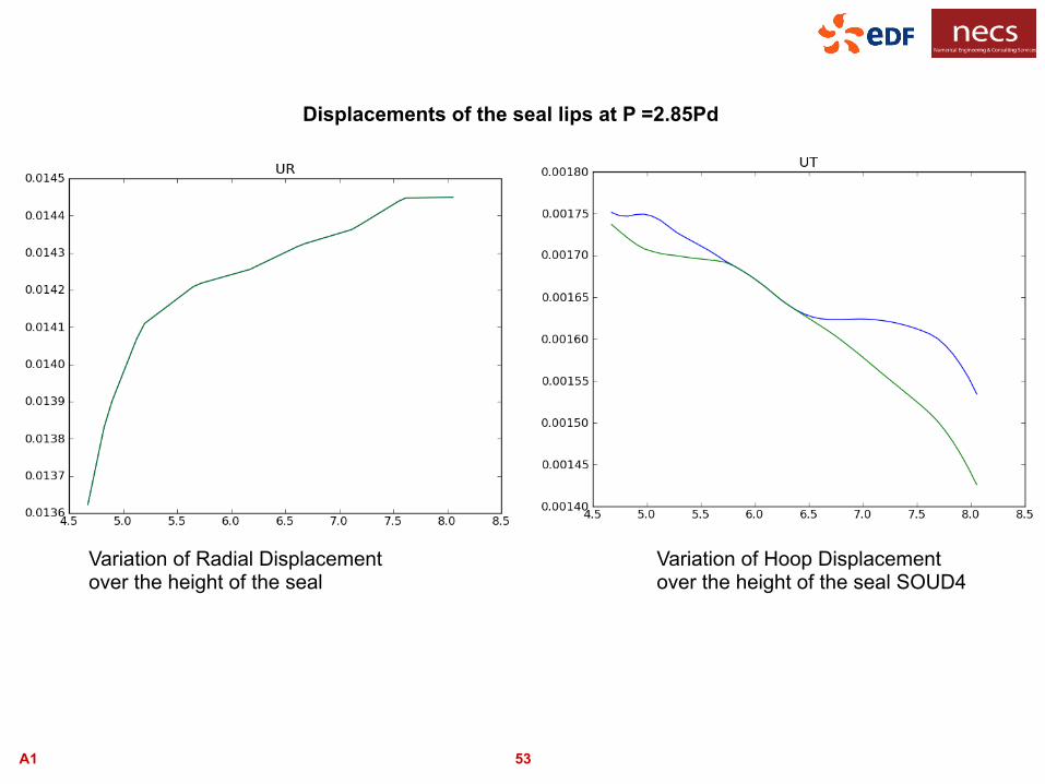
Displacements of the seal lips at P =2.85Pd

Variation of Radial Displacement over the height of the seal

Variation of Hoop Displacement over the height of the seal SOUD4

A1 54

Opening of the SOUD 4: Measure of the displacement jump along the seal length

Normal stress in the cohesive zone element along the seal length

A1 55

Opening of the SOUD 1: Measure of the displacement jump along the seal length

Opening of the SOUD 3: Measure of the displacement jump along the seal length

SOUD4

SOUD1

SOUD3

A1 56

Conclusions

Promissing results of Application of the CZM to the rupture of the Liner: Activation of the various seals. Progressive opening of the seal

Limitations and problems to overcome: Sensitivity to the refinement of the mesh / parameters Sensitivity to the methodology ( displacements imposed ) Overcome convergence problems related to the softening behavior of the CZM law