performance monitoring of a daylit commercial office

ENERGY CENTEROF WISCONSIN

Report Summary210-1

Life-Cycle Energy Costs andGreenhouse Gas Emissions forGas Turbine Power

April, 2002

report report report report report










report report report report reportenergy center

Performance Monitoring of a Daylit Commercial Office Building

February 2003

217-1

The Hoffman Corporation Headquarters

Report 217-1

Performance Monitoring of a Daylit Commercial Office Building

The Hoffman Corporation Headquarters

February 2003

Prepared by

Scott Pigg Senior Project Manager

Ben Sliwinski

Research Associates

595 Science Drive

Madison, WI 53711 Phone: 608.238.4601 Fax: 608.238.8733

E-mail: [email protected] www.ecw.org

Copyright © 2003 Energy Center of Wisconsin All rights reserved

This document was prepared as an account of work conducted by the Energy Center of Wisconsin (ECW). Neither ECW, participants in ECW, the organization(s) listed herein, nor any person on behalf of any of the organizations mentioned herein:

(a) makes any warranty, expressed or implied, with respect to the use of any information, apparatus, method, or process disclosed in this document or that such use may not infringe privately owned rights; or

(b) assumes any liability with respect to the use of, or damages resulting from the use of, any information, apparatus, method, or process disclosed in this document.

Project Manager Scott Pigg Energy Center of Wisconsin

Acknowledgements Mr. Paul Hoffman of the Hoffman Corporation provided his generous support and cooperation. Mr. Ed Erickson and Mr. Tom Cox at Hoffman added their valuable support as Hoffman Corporation points-of-contact for the research team. Mr. Mark Hanson provided many useful comments on early drafts of the results. Mr. Cliff Nitz of Building Automation Technologies, Inc. (BATI) provided outstanding support by volunteering his time and expertise in setting up the building control systems to provide datalogging for the project. Brett Bergee, ECW staff, faithfully retrieved data from the site, and implemented the employee survey. Mr. Earl Van Epren of Schommer Electric provided exceptional support in installed the power monitoring sensors and provided troubleshooting assistance. Mr. Phil Grishaber of Wisconsin Electric was extremely helpful in providing electric and gas data for the Hoffman Building. We also would like to thank Tom Young and Rick Czajka at Wisconsin Electric for their help in installing a Wisconsin Electric pulse output electric meter at the site. Finally, the research team would like to thank the employees of the Hoffman Corporation for their patience and cooperation during this study.

This report is funded by the Wisconsin Department of Administration, Division of Energy and Intergovernmental Relations.

January 2003

Andrea

Contents

Report Summary............................................................................................................................................................1

Introduction ...................................................................................................................................................................2

Findings .........................................................................................................................................................................5 Lighting Energy Use ..................................................................................................................................................5 Chiller Sizing ...........................................................................................................................................................11 Overall Energy Use and End-Use Breakouts ...........................................................................................................14

Conclusions .................................................................................................................................................................17

References ...................................................................................................................................................................19

Appendix A — Monitoring and Analysis Details......................................................................................................A-1 Data Collection System..........................................................................................................................................A-1 Indoor Ambient and Parking Lot Lighting.............................................................................................................A-2 Chiller Analysis .....................................................................................................................................................A-9 Annual Chiller Electricity Use .............................................................................................................................A-10 Fan Systems .........................................................................................................................................................A-11 Carbon Dioxide Monitoring.................................................................................................................................A-15

Appendix B — Survey of Employees........................................................................................................................B-1

1

Report Summary This report presents the results of detailed monitoring of lighting and other energy uses for the Hoffman Corporation headquarters in Appleton, Wisconsin. The Hoffman building was designed to make use of daylighting and reduce the need for interior electric lighting. The 38,700 square foot facility is a two-story building with a clerestory and large north- and south-facing fenestration to admit daylight into several open office bays. Detailed monitoring was conducted of lighting, chiller, and whole facility electricity use in 2001 to examine actual lighting energy use in the Hoffman building, and to investigate issues related to the chiller sizing. A survey of employee satisfaction with the lighting and indoor comfort in the building was also conducted.

The results of the study show that:

• The Hoffman building uses about 0.7 Watts per square foot of lighting energy, which is less than one-half the maximum allowed by Wisconsin code, 37 percent less than the median U.S. office building, and perhaps 25 percent less than the median new office building. Interior lighting represents about 20 percent of the total electricity use for the Hoffman building, compared to a median of 40 percent for all U.S. office buildings.

• Despite the reduced level of ambient electric lighting provided, work station task lights makes up less than 10 percent of the approximately 26 kilowatts of lighting electricity demand in a typical work day, suggesting that the combination of ambient electric lighting and natural daylight is sufficient at most work stations. Light level monitoring at sampled workstations showed at least 20 footcandles on work surfaces, and work stations closer to the exterior showed higher light levels.

• A survey of employees at the Hoffman building showed a high level of satisfaction with the quality of lighting at the facility. Some workers near the windows find the light level to be unacceptably bright and have troubles with glare, and there is dissatisfaction with the lighting in a small windowless work area in the basement of the building. But 70 percent of the 71 survey respondents rated the overall quality of light at their workstation as “good” or “very good.”

• Analysis of overall electricity and natural gas use by the facility indicates that the Hoffman building is about average to somewhat above average in terms of overall energy use per square foot compared to other U.S. office buildings. There are indications that energy use by ventilation fans in the Hoffman building is much higher than average, which may be offsetting the lighting energy savings. (High fan electricity use was later traced to a programming error in the building automation system). It is also possible that higher-than average plug loads in the building may offset the electricity savings from the daylighting.

• The 102-ton chiller for the Hoffman building may be somewhat oversized, but not substantially so. The existing chiller is larger than the 70- to 80-ton chiller that would be called for based on daylighting program guidelines. During the period of monitoring, sustained chiller load of about 80 tons was observed on one particularly hot day that exceeded the design conditions for the site. At the same time, there are indications that the ventilation rate in the building may be on the high side, which may add 10 tons or more to the chiller load on hot humid days. A 90-ton chiller could easily meet the building load, even at the observed high ventilation rate. A 70- to 80-ton chiller might be adequate for the building, but would require better control of the ventilation system, and would allow little margin for future growth in internal loads (the building is not currently completely occupied).

2

Introduction

Background The Hoffman Corporation is an architectural, engineering, and construction firm headquartered in Appleton Wisconsin. In January 2000, the company moved into a new 38,689 square-foot facility, that incorporates green building construction and design features including extensive use of daylighting. The building serves as a showcase of green building and daylighting technologies. The facility has two floors above grade and a basement area (Figure 1). Nearly all workstations are located in open areas in the east and west wings of the two above-ground floors (there are only two private offices in the building). A few workstations are located in a windowless area in the basement, which also contains the mechanicals room, kitchen facilities, storage, a large meeting room, and an exercise room. Ambient lighting in the facility is provided mostly by suspended direct/indirect T-8 fluorescent fixtures, which were designed to provide 20 foot candles of illumination at desk level. The lighting is controlled by a central lighting controller with scheduled on/off times. Under-cabinet fluorescent task lighting is also provided for the workstations. A central two-stage, air-cooled 102-ton chiller provides space cooling. Heating is provided by two one-million BTU/hr high efficiency boilers. The facility uses variable-air-volume (VAV) air delivery with hot water reheat, and the building uses three air handlers with separate supply and return fans. The air handlers are equipped with variable-speed drives.

Objective Beginning in May of 2001, the Energy Center of Wisconsin initiated detailed energy-use monitoring at the Hoffman building meant to document energy use at the facility. The primary objective of the study was to assess lighting energy use. The extensive use of daylighting throughout the facility is expected to result in reduced electric lighting loads in the building, with a concomitant reduction in the need for space cooling. A secondary objective was to assess chiller sizing for the facility. Though the facility makes extensive use of daylighting—which should result in reduced heat gain from internal lighting—the existing chiller is sized somewhat larger than program standards would call for.

3

Figure 1, Hoffman building views and schematic. Clockwise from upper left: south face of building; west face of building; schematic showing approximate use of space; second floor work station.

Second Floor

First Floor

North

WorkStations

WorkStations

WorkStations

WorkStations

WorkStations

ReceptionArea

Conference Rooms

Open to below

Main Entrance

Stairwell/Elevator

Second Floor

First Floor

North

WorkStations

WorkStations

WorkStations

WorkStations

WorkStations

ReceptionArea

Conference Rooms

Open to below

Main Entrance

Stairwell/Elevator

4

Approach The monitoring conducted for the project included a combination of data collection from parameters tracked by the building’s energy management system (EMS) and stand-alone metering. Monitored points included:

• whole building electricity use • chiller electricity use • ambient lighting electricity use • electricity use for task lighting at sampled workstations • light levels at sampled workstations • temperature, relative humidity, and carbon dioxide concentrations (September – January only) • operational status of HVAC equipment such as air handlers and boilers

More details on the monitoring conducted can be found in Appendix A. In addition to detailed energy monitoring, this report also makes use of monthly utility usage records for the Hoffman building. Finally, a survey of employees was conducted in December 2201 to explore occupant satisfaction with the lighting and general indoor environment in the building. The survey instrument and tabulated responses are included in Appendix B.

5

Findings

Lighting Energy Use

Ambient Lighting Ambient lighting in the Hoffman building is provided by direct/indirect fluorescent lighting (T8, electronic ballast) suspended from the ceiling. Additional lighting on the second floor is provided by fluorescent uplighting in the clerestory. The lighting is designed to provide at least 20 footcandles of light on work surfaces. All ambient fluorescent lighting in the building has bi-level switching capability, and open-area lighting is time-clock controlled to ensure shut-off. Occupancy sensors control lighting in conference rooms and the few private offices in the building.

Power for ambient lighting is provided through “east” and “west” circuit panels, which also provide power for parking lot lighting. For the study, total power through each panel was monitored on a 15-minute basis, and separate monitoring was installed to detect whether the parking lot lighting was on or off. Additional details from the ambient lighting monitoring can be found in Appendix A.

Figure 2 shows the average weekday time-of-day profile for total ambient lighting in the building (excluding the parking lot lighting). The profile shows a fairly steady demand averaging about 25 kW during the day. This weekday in-use lighting demand works out to about 0.65 Watts per square foot, which is less than one-half of the maximum lighting power density allowed by Wisconsin code for offices (1.5 Watts per square foot).

Figure 2, Average weekday demand for interior ambient lighting.

Mean Kilowwatts

0

5

10

15

20

25

30

6am 8am 10am Noon 2pm 4pm 6pm

6

Workstation Task Lighting Most workstations in the Hoffman building have built-in task lighting, and some employees have added table lamps and other types of task lights. The typical workstation has two fluorescent under-cabinet task lights, with a total connected load of about 60 Watts.

To examine electricity use for task lighting, we monitored a random sample of ten workstations each month. In all, 66 workstations were monitored between late May 2001 and early January 2002. Appendix A describes the sampling and monitoring of task lighting in more detail.

The results show that about half of the employees do not use their task lights at all during office hours, and few employees use all of the task lighting available to them (Figure 3). Averaging the data to yield a time-of-day profile across all monitored workstations reveals an average of about 15 to 17 Watts of task lighting use per workstation during working hours (Figure 4). When multiplied out by the in-use workstations in the facility, the data indicate a total of about 1.6 kW of task lighting load for the building. No readily apparent seasonal trend is evident from the data, but the nature of a rotating sample of workstations makes such analysis difficult.

0

10

20

30

40

50

60

70

80

Workstation withleast task lighting use

Workstation withmost task lighting use

Mean Watts (9am – 5pm weekdays), by workstation

0

10

20

30

40

50

60

70

80

Workstation withleast task lighting use

Workstation withmost task lighting use

Mean Watts (9am – 5pm weekdays), by workstation

Figure 3, Distribution of workstation task lighting use.

0 2 4 6 8 10 12 14 16 18 20 22 24

0

5

10

15

Mean Watts per workstation

Hour of Day0 2 4 6 8 10 12 14 16 18 20 22 24

0

5

10

15

Mean Watts per workstation

Hour of Day

Figure 4, Average weekday demand profile for task lighting.

7

Overall Lighting Demand and Energy Use Combining the data on ambient and task lighting use yields the estimates of typical weekday (and weekend) total lighting demand and energy use shown in Table 1 and Figure 5. Clearly, the ambient lighting makes up the majority of electric lighting load in the building.

Table 1, Average interior lighting demand and energy use.

Peak Demand

Daily Energy Use

kW Watts per ft2 kWh Weekdays

Interior ambient lighting 25.5 0.65 367.1 Workstation task lighting 1.6 0.04 16.6

Total 27.1 0.70 383.7 Weekends and holidays

Interior ambient lighting 3.8 0.10 68.3 Workstation task lighting 0.2 <0.01 3.7

Total 4.0 0.10 72.0

Mean Kilowatts

0

5

10

15

20

25

30

6am 8am 10am Noon 2pm 4pm 6pm

Ambient Lighting

Task Lighting

Figure 5, Average weekday demand for interior lighting, including ambient and estimated task lighting load.

8

Assuming an average of 251 non-holiday weekdays per year, the figures in Table 1 work out to annual lighting energy use of about 105,000 kWh per year, or 2.70 kWh per square foot, whick represents about 20 percent of the total electricity use in the building.

To gauge how this usage compares to other office buildings around the country, we compared the Hoffman building lighting use per square foot to a publicly available sample of office buildings in the 1995 Commercial Building Energy Consumption Survey (CBECS) conducted by the federal Energy Information Administration (EIA, 1998).1 This nationwide set of data contains information on 1,226 commercial buildings categorized as “office/professional.” Note that lighting energy use was not directly monitored for these buildings, but was estimated by statistically adjusting building energy use simulations of electrical end uses to actual utility records of overall electricity usage.

The Hoffman lighting use of 2.70 kWh per square foot is about 37 percent lower than the median CBECS estimate for all office buildings (4.3 kWh/ft2), with the Hoffman building ranking at the 29th percentile among the 1,226 office buildings in the CBECS dataset. Compared to the 103 new office buildings in the data set (i.e., those constructed in 1990 or later), the Hoffman lighting use ranks at about the 20th percentile, or 25 percent below the median of 3.6 kWh per square foot. The small sample size—and the amount of weight assigned to each building in the CBECS data—makes the latter comparison more tenuous, however. Nevertheless, the analysis suggests that lighting energy use at the Hoffman building is considerably below that of the typical U.S. office building.

Another point of comparison is a non-residential baseline study conducted in California in 1999 (NBI, 2001; RLW Analytics, 1999). For that study, on-site audits of lighting equipment and operating schedules were used to estimate annual lighting energy use for new office buildings (among other categories of new commercial buildings). The figures derived here for the Hoffman building are about 32 percent lower than the 4.0 kWh/ft2 annual electric lighting use estimated for California office buildings in that study.

1See: http://www.eia.doe.gov/emeu/cbecs/microdat.html.

9

Light Levels

A data logging light meter was left at one randomly-sampled workstation each month between May 2001 and January 2002 (see Appendix A for sampling details). The light meter provided 4-minute interval samples of light levels for the sampled workstations. Figure 6 shows the weekday light-level profiles for the sampled workstations. The profiles indicate that the design level of 20 footcandles is maintained in the core of the building. Light levels are substantially higher at workstations near windows, and at least two workstations (Round 2 and Round 6) show evidence of direct sunlight at times during the day.

Second Floor

First FloorNorth

Round 1,Workstation 95/19 – 6/21







0 6 12 18 240

10

20

30

0 6 12 18 240

100

200

300

0 6 12 18 240

20

40

60 0 6 12 18 240

10

20

0 6 12 18 240

5

10

15

20

0 6 12 18 240

50

100

0 6 12 18 240

10

20

30

40

Mean Footcandles (weekdays)

Hour of Day

Second Floor

First FloorNorth








0 6 12 18 240

10

20

30

0 6 12 18 240

10

20

30

0 6 12 18 240

100

200

300

0 6 12 18 240

100

200

300

0 6 12 18 240

20

40

60

0 6 12 18 240

20

40

60 0 6 12 18 240

10

20

0 6 12 18 240

10

20

0 6 12 18 240

5

10

15

20

0 6 12 18 240

5

10

15

20

0 6 12 18 240

50

100

0 6 12 18 240

50

100

0 6 12 18 240

10

20

30

40

0 6 12 18 240

10

20

30

40

Mean Footcandles (weekdays)

Hour of Day

Figure 6, Monitored light levels at sampled workstations.

10

Perceived Quality of Lighting In December 2001, a short survey of employees at Hoffman was conducted to obtain information on perceptions of lighting quality and indoor comfort at the

Hoffman building. A total of 131 questionnaires were distributed, of which 71 were completed and returned. The full instrument and tabulated responses can be found in Appendix B; here we cover only the findings regarding lighting.

Figure 7 shows the overall ratings given by the respondents regarding the quality of light at their workstation. A majority of respondents rated the light quality as “good” or “very good.” Only six respondents rated the quality of light as “poor,” and three of these respondents worked in a windowless basement area of the building. If the seven respondents from the basement area are excluded, fewer than 5 percent of respondents rated the quality of light at their workstation as poor, and 73 percent rated it as “good” or “very good.”

A total of 13 respondents (18 percent) said that glare was a problem most or all of the time when working on their computer or reading. Other than the fact that all but one of the respondents were within two workstations of a window, there was no clear clustering of these respondents by floor or wing of the building.

Eleven respondents (16 percent) rated the amount of light at their workstation as either a little too dim (9 respondents) or much too dim (2 respondents). The windowless basement area of the building garnered a significantly higher proportion of respondents who felt the lighting was too dim (3 out of 6 respondents to this question), and was also the location of the two respondents who said the lighting was much too dim.

Similarly, eight respondents (11 percent) rated the light at their workstation either a little too bright (6 respondents) or much too bright (2 respondents). Seven of these respondents worked on the second floor, though this proportion is not statistically significantly different than the other floors due to the small sample size and the fact that more than half of the respondents overall were located on the second floor. The two respondents who felt the light level was much too bright both worked on the south face of the building directly across from the main windows.

Poor8%

Average21%

Good43%

Very Good28%

Overall,…how would you rate the quality of light at yourWorkstation? (n=71) Poor

8%

Average21%

Good43%

Very Good28%

Overall,…how would you rate the quality of light at yourWorkstation? (n=71)

Figure 7, Employee satisfaction with lighting.

11

Chiller Sizing One of the questions to be addressed in this study is whether the Hoffman Building chiller is oversized, and if so, by how much. The Hoffman Building chiller is a 102 ton nominal capacity air-cooled water chiller. Chillers serving conventional office buildings are typically sized at 300 to 400 square feet of floor space per ton of chiller capacity. A daylit building such as the Hoffman building is expected to have reduced internal gains from electric lighting, and can typically be sized at 500 square feet per ton or more, according to current program standards. At 379 square feet per ton, the Hoffman chiller is close to the high end of square feet per ton of capacity for a conventional building, but below the recommendations for a daylit building. A guideline of 500 square feet per ton would call for 77 tons of chiller capacity for the Hoffman building. For the study, we used monitored electrical demand for the chiller to estimate delivered cooling output. The rated maximum electrical demand for the chiller compressors for the Hoffman building is 124 kW. The chiller also has ten 1-horsepower condenser fans. Electrical demand for the condenser fan motors is estimated at .83 kW per motor assuming 90 percent motor efficiency. Assuming that all fans are running at peak cooling load, the estimated total peak electric demand for the chiller plus condenser fans is approximately 132 kW, or about 1.3 kW/ton. Data analyzed here were collected from Late May through mid-September, though some data are missing due to problems with the EMS system in August. Figure 8 shows the 15-minute chiller demand and associated weather data (from the nearby Appleton airport) during three of the hottest days for which usable data were obtained. The data show high demand in the early morning as the chiller recovers the building from the higher overnight setpoint. The system then shows reduced— but increasing—demand through the remainder of the morning and into the afternoon as outdoor temperature climbs. The system typically shuts down at about 5 pm, but shows some demand in the evening, perhaps in response to manual thermostat adjustments by cleaners or employees working late. The data indicate chiller demand rising to slightly more than 100 kW during the afternoon on July 31, which suggests that the chiller was delivering about 80 tons of cooling capacity at that time. The chiller load was somewhat lower on the following two days, which were slightly cooler. As bottom graph in Figure 8 shows, afternoon air temperatures met or exceeded the 1% design conditions for Appleton during these three days, and the dewpoint was consistently about five degrees above design conditions. Regression analysis of afternoon chiller demand versus weather data (see Appendix A) suggests that the chiller would be delivering in the range of 60 to 70 tons of cooling on afternoons at 1 percent design conditions.2

2 Subsequent to review of a draft version of this report, the building operations subcontractor informed us that shortly after the completion of monitoring for this project, a large amount of fluff from nearby cottonwood trees was removed from the chiller condenser coils. This may have affected chiller performance over the monitoring period for the project.

12

60

70

80

90

100

midnight noon midnight noon midnight noon midnight

Temperature [F]

Observed Dry bulb

Observed Dew Point

Design dry bulb

Design dew point

(Note: design conditions are Appleton 1% coincident conditions.Source: ASHRAE, 1993)

0

25

50

75

100

125

0

20

40

60

80

100

Kilowatts Tons

July 31 August 1 August 2

Maximum output (132 kW, 102 tons)

July 31 August 1 August 2

midnight noon midnight noon midnight noon midnight

60

70

80

90

100

midnight noon midnight noon midnight noon midnightmidnight noon midnight noon midnight noon midnight

Temperature [F]

Observed Dry bulb

Observed Dew Point

Design dry bulb

Design dew point

(Note: design conditions are Appleton 1% coincident conditions.Source: ASHRAE, 1993)

0

25

50

75

100

125

0

20

40

60

80

100

Kilowatts Tons

July 31 August 1 August 2July 31 August 1 August 2

Maximum output (132 kW, 102 tons)

July 31 August 1 August 2July 31 August 1 August 2

midnight noon midnight noon midnight noon midnightmidnight noon midnight noon midnight noon midnight

Figure 8, Chiller demand (top) and temperatures (bottom), July 31 through August 2.

13

However, our monitoring also shows some evidence that the HVAC system is delivering a rather large amount of outdoor air to the building. High ventilation rates are good for indoor air quality, but impose additional burden on the HVAC system, which must cool and dehumidify more outdoor air.

The evidence for a high ventilation rate in the Hoffman building comes from indoor carbon dioxide concentration data collected from September 2001 through early January 2002 at 30-minute intervals for five locations in the building. Carbon dioxide concentration is commonly used to estimate ventilation rates in buildings, because at equilibrium, indoor CO2 concentration is related to the amount of outdoor air provided per person. Low ventilation rates result in high CO2 concentrations; high ventilation rates result in low CO2 concentrations.

Wisconsin commercial building code requires that at least 7.5 cfm of outdoor air be provided per occupant, which corresponds to an equilibrium indoor concentration of 1,900 parts per million (ppm), assuming 400 ppm outdoor CO2 concentration and a CO2 generation rate typical of office workers (0.011 cfm per person). Other guidelines call for 15 cfm per person, which would correspond to about 1,100 ppm indoor concentration under the same assumptions.

As Figure 9 shows though, CO2 levels rarely exceeds even 600 ppm in the Hoffman building, suggesting an average ventilation rate that is much higher than typical design guidelines. Even after correcting for the fact that equilibrium conditions may not be achieved over the course of the day (see Mudarri, 1997), the data suggest a ventilation rate of at least 50 cfm per person in the building. Under design conditions, the difference between 15 and 50 cfm per person of ventilation could be expected to add about 12 tons of cooling load to the chiller.3

3 Assumptions are as follows: occupancy, 100 people; outdoor air at 89oF with 68 oF dewpoint; indoor air at 75 oF at 50% relative humidity.

Figure 9, Mean hourly indoor carbon dioxide concentration.

300

400

500

600

700

800

0 2 4 6 8 10 12 14 16 18 20 22

Carbon Dioxide Concentration (ppm)(average of five locations)

25th percentile

75th percentilemedian

5th percentile

95th percentile

outliers

Hour of Day

Note: weekends and holidays excluded300

400

500

600

700

800

0 2 4 6 8 10 12 14 16 18 20 22

Carbon Dioxide Concentration (ppm)(average of five locations)

25th percentile

75th percentilemedian

5th percentile

95th percentile

outliers

Hour of Day

Note: weekends and holidays excluded

14

Overall Energy Use and End-Use Breakouts

Analysis of monthly utility billing records (Figure 9) indicates that the Hoffman building uses about 16,500 therms of natural gas and 500,000 kWh of electricity in a year with average weather (see weather correction analysis details in Appendix A). This works out to about 0.42 therms per square foot of natural gas and 12.9 kWh per square foot of electricity.

As with lighting energy, we compared the Hoffman whole-building electricity and natural gas use per square foot to the 1995 CBECS sample of office buildings. Ideally, one would compare energy use for the Hoffman building with other new office buildings of comparable square footage in similar climate zones. However, the national sample of 1,226 office buildings in the sample quickly becomes unacceptably small when these restrictions are simultaneously applied.

Therefore, we instead compared energy use for the Hoffman building with various less restrictive subsets of the CBECS sample in Table 2. The results suggest that the Hoffman building as operated during the monitoring period is average to somewhat higher than average in terms of electricity and natural gas use per square foot.

Of course this does not necessarily mean that the energy efficiency strategies employed in the design of the Hoffman building are not effective; energy efficiency savings for some end-uses may be offset by higher-than-average energy use for computers or other equipment by engineering firms such as Hoffman.

At the same time, comparison of the Hoffman building usage with the national CBECS data at the end-use level suggests that higher-than-average fan electricity use lies at the heart of why total electricity use by the facility is somewhat above average despite having demonstrably lower lighting energy. By our analysis, fans make up about 30 percent of the Hoffman building electricity use, compared to only 4 to 5 percent of electricity use for typical office buildings (Figure 11). Moreover, when electricity use per square foot is broken into categories that can be compared between the Hoffman monitoring data and the CBECS database, the results suggest substantially higher-than-typical fan energy use for the Hoffman building, but comparable space cooling and other uses (Figure 12).

The forgoing analysis is somewhat uncertain, since we did not directly observe fan electricity use (see Appendix A), and (as noted previously) the CBECS estimates of end-use electricity consumption are statistically derived rather than directly measured. Nonetheless, taken with the observed low CO2 levels in the building, the data tend to suggest that the fan systems are not being optimally controlled for electricity consumption.4

4 Indeed, after reviewing a draft version of this report, the building operations subcontractor found an error in the control algorithm for the air handlers that caused one or more air handlers to run at full output at night.

0

10,000

20,000

30,000

40,000

50,000

60,000

70,000

Jan Feb Mar Apr May Jun Jul Aug Sep Oct Nov Dec

Ele

ctric

ity (k

Wh)

0

500

1,000

1,500

2,000

2,500

Nat

ural

Gas

(the

rms)

Electricity

Natural Gas

Figure 10, Hoffman building monthly electricityand natural gas use (2001).

15

Table 3, Comparison of Hoffman energy use with CBECS.

Electricity Use Natural Gas Use

(Hoffman building: 12.9 kWh/ft2) (Hoffman building: 0.42 therms/ft2)

1995 CBECS

n

1995 CBECS median kWh/ft2a

Hoffman rank among

CBECS buildings

(percentile)a

1995 CBECS

nb

1995 CBECS median

therms/ft2 a

Hoffman rank among

CBECS buildings

(percentile) a

Nationwide

All office buildings 1226 12.2 57 741 0.33 61

New construction onlyc 103 10.7 65 62 0.21 65

5,000-100,000 square feet only 607 13.1 50 380 0.27 78

New construction and 5,000-100,000 square feet

46 9.4 56 31 0.21 94

Cold Climate Zoned

All office buildings 82 7.5 73 50 0.7 18

5,000-100,000 square feet only 50 12.9 51 31 0.4 57

aAnalysis uses CBECS case weights.

bIncludes only office buildings that use natural gas.

c New construction defined as buildings constructed between 1990 and 1995.

dCold climate zone defined as >7,000 heating degree days and <2,000 cooling degree days

16

Interior Lighting

21%

Parking Lot Lighting

3%

Chiller13%

Fans31%

Other32%

0

1

2

3

4

5

6

7

Interior Lighting Space Cooling Fans Other

Hoffm

an

CBECS*

All

5-10

0 K

ft2

New

5-10

0 K

ft2 an

d ne

w

kWh

per s

quar

e fo

ot

*CBECS values are medians using CBECS case w eights.

0

1

2

3

4

5

6

7

Interior Lighting Space Cooling Fans Other

Hoffm

an

CBECS*

All

5-10

0 K

ft2

New

5-10

0 K

ft2 an

d ne

w

kWh

per s

quar

e fo

ot

*CBECS values are medians using CBECS case w eights.

Figure 12, Hoffman building electric end-use intensities, compared to CBECS median values.

Figure 11, Electricity end-use proportions for the Hoffman Building.

17

Conclusions The daylighting strategy pursued at the Hoffman building has resulted in lighting electricity use at the facility that is substantially less than both Wisconsin code and what is typical for a U.S. office building. The reduced ambient electric lighting use has not come at the expense of significant task lighting use or employee dissatisfaction with the quality of lighting in the building. Despite having clearly lower lighting loads, overall energy use at the Hoffman building appears to be about average or even somewhat above average for an office building—though our basis for comparison (the national CBECS database) is substantially broader than the population of new Wisconsin office buildings. Something appears to be offsetting the lighting and related space-cooling savings from daylighting. To us, the evidence points toward a fan systems that are not optimized for energy use. Though both our estimates of ventilation electricity use in the Hoffman building and the estimates of ventilation energy use in the CBECS sample have considerable uncertainty, some hard data that we collected also point in the direction of high fan energy use. These are: (1) very low measured carbon dioxide levels that indicate high ventilation rates; and, (2) data from air handler variable speed drives that shows one (and sometimes two) air handlers running at full speed all night every night. The other possibility is that it is higher-than-average plug loads and other miscellaneous uses of electricity that offset the lighting savings for the Hoffman building. It is possible that as an design-build firm, the Hoffman Corporation employees use more computers and use them more intensively than in other office environments. Though our measure of “other” electricity use for the Hoffman facility tends to match up well with the CBECS figures, if we have somehow overestimated fan system electricity use (which we did not measure directly, but estimated from air handler speed data), then we would have commensurately underestimated electricity use in the “other” category. The 100-ton chiller at the facility does appear to be somewhat oversized. But the facts of the matter are difficult to sort out, and it is possible to argue for just about any size between 60 and 90 tons. First there is the issue of the appropriate design conditions. We initially took the ASHRAE 1% summer conditions to be the appropriate design point, which would call for 60 to 70 tons of chiller capacity based on the data we observed. But our monitoring during the summer of 2001 included several days in a row that exceeded these conditions. In particular, we observed one day during which 80 tons of chiller capacity was required over the course of the afternoon. But at the same time, there are indications that the ventilation system is not running in an optimal manner, resulting in substantial added chiller load from outdoor air being introduced into the building. Reducing the amount of outdoor air introduced into the building during peak cooling conditions might reduce the load on the chiller by 10 tons or more. On the other hand, the building is not at full occupancy (we would ballpark it at perhaps 80 to 90 percent occupied), and additional chiller load from more people and computers could occur in the future. Finally, we would make the distinction between establishing chiller size in retrospect, when loads can be measured, and specifying a chiller based on a set of blueprints when the building is being designed. The latter necessarily includes substantial uncertainty which, taken conservatively, means erring on the high side rather than the low. So while it is possible to argue for a 60 to 70-ton chiller—which would require better optimization of the ventilation

18

system, would not allow for future load growth, and which might experience some days during the summer during which it could not completely meet the load—we would argue that 80 to 90 tons is a more realistic value. We have three specific recommendations as a result of this study that are directly related to the operation of the Hoffman facility: 1. We recommend that the Hoffman Corporation investigate the control strategies for outdoor air

ventilation and fan system operation. Air handler electricity use appears to be high, and it appears that a large amount of outdoor air is being introduced into the building. Optimization of these systems might result in substantial electricity savings.

2. Additional lighting energy savings could be obtained by installing photosensor controls for the ambient lighting in the open office bays. These would shut off banks of ambient lighting near the windows when adequate daylight is present.

3. There are some aspects of the chiller system control that could be optimized to reduce on-peak demand charges. We observed one occasion where the morning chiller recovery period slipped a few minutes past 9 a.m., resulting in a hefty on-peak demand charge and established a new high for the rolling 11-month demand charge. Similarly, there have been brief evening spikes of high chiller demand that occurred during on-peak periods, as well as periods during the fall shoulder season when the chiller operated briefly at high loads.

Our final recommendation is a broader one related to commercial building research. The most significant limitation of this project has to do not with the data that we collected from the Hoffman building, but rather the lack of a good basis for comparing the Hoffman facility to other similar office buildings. The CBECS dataset that we used for this purpose is indeed a rich set of data, but it represents a much broader geographic area and is not specific to new buildings. Given the program emphasis in Wisconsin on high performance commercial buildings in the state, we believe it would be beneficial to establish some benchmarks for energy use among new office buildings in Wisconsin. The effort could be as simple as establishing a distribution of whole-building electricity and gas use per square foot for a sample of Wisconsin office buildings based on utility data (though more detailed information on end-use intensities would be more helpful). Such data would help lend credibility to the high performance building effort in Wisconsin.

19

References [EIA] Energy Information Administration. 1998. A Look at Commercial Buildings in 1995: Characteristics, Energy Consumption, and Energy Expenditures. DOE/EIA-0625(95).

Mudarri, David H. 1997. “Potential Correction Factors for Interpreting CO2 Measurements in Buildings,” ASHRAE Transactions, vol. 103, Pt. 2.

New Buildings Institute (NBI). 2001. Advanced Lighting Guidelines, 2001 Edition. New Buildings Institute. www.newbuildings.org.

RLW Analytics. 1999. “Non-Residential New Construction Baseline Study,” final report prepared for Southern California Edison. (See www.calmac.org).

A-1

Appendix A — Monitoring and Analysis Details

Data Collection System The data collection system in place at the Hoffman Building makes use of a number of components. These include: • the building's KMC digital energy management and control system • Veris Enercept power sensors installed on lighting, and chiller circuits • a Wisconsin Electric pulse output whole building electric meter • Brultech power sensors installed on task lighting for a sample workstations • HOBO time of use sensors installed on parking lot lighting

EMS System Monitoring The data logging feature of the KMC energy management system provides data logging of lighting and chiller power from sensors installed on the lighting and chiller circuits. It also performs pulse counting and data logging of the pulse data provided by the Wisconsin Electric whole building electric meter. A summary of the data collected by the EMS system for this effort is provided in the table below, which is organized in terms of the data panels, logs and variables from the EMS system that were tracked for the project.

Table A1, Summary of Points Monitored by EMS at Hoffman Building

EMS Panel Log Description Variable 1 Variable 2 Variable 3 Variable 4 A10 TL1 West Lights KWh kW TL2 East Lights KWh kW TL3 Chiller KWh kW TL4 Supply Fan 1 (AC1-VFD) % Speed TL5 Supply Fan 2 (AC2-VFD) % Speed TL6 Supply Fan 3 (AC3-VFD) % Speed TL7 Pumps P1, P2, P4 P1/P2 % Speed P4 % Speed TL8 Pumps IP1, IP2, P3 IP1 Amps IP2 Amps P3 Status A15 TL1 TPM107 Southwest VAV RHT-VLV Room Temp Room STPT CFM A26 TL1 TPM120 Southeast VAV RHT-VLV Room Temp Room STPT CFM A33 TL1 TPM207 South VAV RHT-VLV Room Temp Room STPT CFM A44 TL1 TPM214 South VAV RHT-VLV Room Temp Room STPT CFM A55 TL6 Chiller Temperatures CWS CWR Outside Air Chiller

Status A56 TL1 Building Power Pulse Total TL7 Boiler Data HWST HWRT Boiler 1

Status Boiler 2 Status

RL1 Boiler 1 Run time Time on Time off RL2 Boiler 2 Run time Time on Time off

A p p e n d i x A

A-2

Indoor Ambient and Parking Lot Lighting Lighting at the Hoffman Building was monitored on two breakers, designated in this report as the West circuit and the East Circuit. These circuits include parking lot lighting. In order to separate parking lot light electrical energy consumption from that of the interior lights, sensors were placed on the parking lot lighting sub-panel to record the times they turned on and off each day. Wattage for the parking lot lights was determined by examining West and East lighting data for weekends. The data consistently showed that the West parking lot lights have a demand of about 3.45 kW while the East lights have a demand of about 2.98 kW, though the on/off times of the parking lot lighting varied over the course of the year with the length of the day.

Lighting Daily Energy Use The seasonal trend in daily electrical energy consumption for the two lighting circuits combined is shown in Figure A1. Weekday lighting energy consumption for the two circuits combined is between 350 and 450 kWh/day, with a slight seasonal trend to increasing consumption with shorter days evident in the data. Weekend data indicate consumption around 100 to 150 kWh/day. Variation in the length of time the parking lot lighting is illuminated appears to drive much of the overall seasonal variability.

Figure A1, Daily lighting kWh (interior and parking lot lighting).

0

100

200

300

400

500

June July August September October November December

Daily kWh

Weekdays

Weekends

0

100

200

300

400

500

June July August September October November December

Daily kWh

Weekdays

Weekends

A p p e n d i x A

A-3

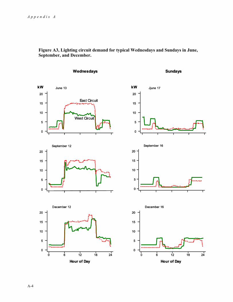
Lighting Demand Profiles Figure A2 shows the overall average weekday and weekend demand profile for the combined lighting circuits. The profile shows fairly level demand during the middle of the day, but varying demand in the mornings and evenings. This is a consequence of averaging in the parking lot lighting, which turns on and off at varied times throughout the year. Figure A3 shows typical Wednesday and Sunday lighting circuit demand for days in June, September and December. The figure shows generally how the parking lot lighting affects the overall demand profile as the day length increases. Figure A3 also shows that the East and West parking lot lights do not come on at the same time of day.

Hour of Day0 2 4 6 8 10 12 14 16 18 20 22 24

0

5

10

15

20

25

30

Mean kW

Weekdays

Weekends

Hour of Day0 2 4 6 8 10 12 14 16 18 20 22 24

0

5

10

15

20

25

30

Mean kW

Weekdays

Weekends

Figure A2, Overall average lighting demand profile (includes parking lot lighting).

A p p e n d i x A

A-4

Figure A3, Lighting circuit demand for typical Wednesdays and Sundays in June, September, and December.

December 16

0 6 12 18 240

5

10

15

20

December 12

0 6 12 18 240

5

10

15

20

September 16

0

5

10

15

20

September 12

0

5

10

15

20

Jjune 17

0

5

10

15

20

June 13

0

5

10

15

20

West Circuit

East Circuit

kW kW

Hour of Day Hour of Day

Wednesdays Sundays

December 16

0 6 12 18 240

5

10

15

20

December 12

0 6 12 18 240

5

10

15

20

September 16

0

5

10

15

20

September 12

0

5

10

15

20

Jjune 17

0

5

10

15

20

June 13

0

5

10

15

20

West Circuit

East Circuit

kW kW

Hour of Day Hour of Day

Wednesdays Sundays

A p p e n d i x A

A-5

Parking Lot Lighting Parking lot lighting on and off times were recorded using a Veris H608 Current Status Switch connected to a HOBO state logger. One switch was placed on the East parking lot lighting circuit and one was placed on the West circuit. A typical segment of data for a single day is shown in the table below. It illustrates a small anomaly in the operation of the East and West circuit lighting controller.

Table A2, Sample data from parking lot monitoring.

East Parking West Parking

Date Time State Elapsed

Time Date Time State Elapsed

Time 6/1/01 4:10:08 On 6/1/01 3:18:12 On 6/1/01 5:25:11 Off 1:15:03 6/1/01 5:18:16 Off 2:00 6/1/01 19:33:09 On 6/1/01 20:41:14 On 6/1/01 23:29:12 Off 3:56:03 6/1/01 23:37:18 Off 2:56

Note that in the morning the East lighting comes on about an hour after the West lighting and stays on for about an hour, while the West lights are on for two hours. In the evening the East lights turn on about an hour before the West lights and stay on for about four hours compared to about three hours for the West lights. Overall, each day the East lights are on for 15 minutes longer than the West lights. The lighting controller computer uses an astronomical calculation to determine sunrise and sunset times for Appleton latitude and longitude and uses this information to determine the times for turning the lights on and off. The amount of time each day the lights stay on varies throughout the year. Power consumption for parking lot lighting was determined by analysis of weekend East and West lighting circuit data obtained through the Veris Enercept power sensors and the KMC EMS system. Figure A3 shows typical weekend demand profiles. On and off times observed in the EMS data were confirmed using the HOBO sensor data.

Based on data for several weekends average consumption for parking lot lights was determined to be 2.98 kW for East lights and 3.45 kW for West lights. These values combined with the on and off times recorded by the HOBO logger allowed removal parking lot lights from the overall demand data.

A p p e n d i x A

A-6

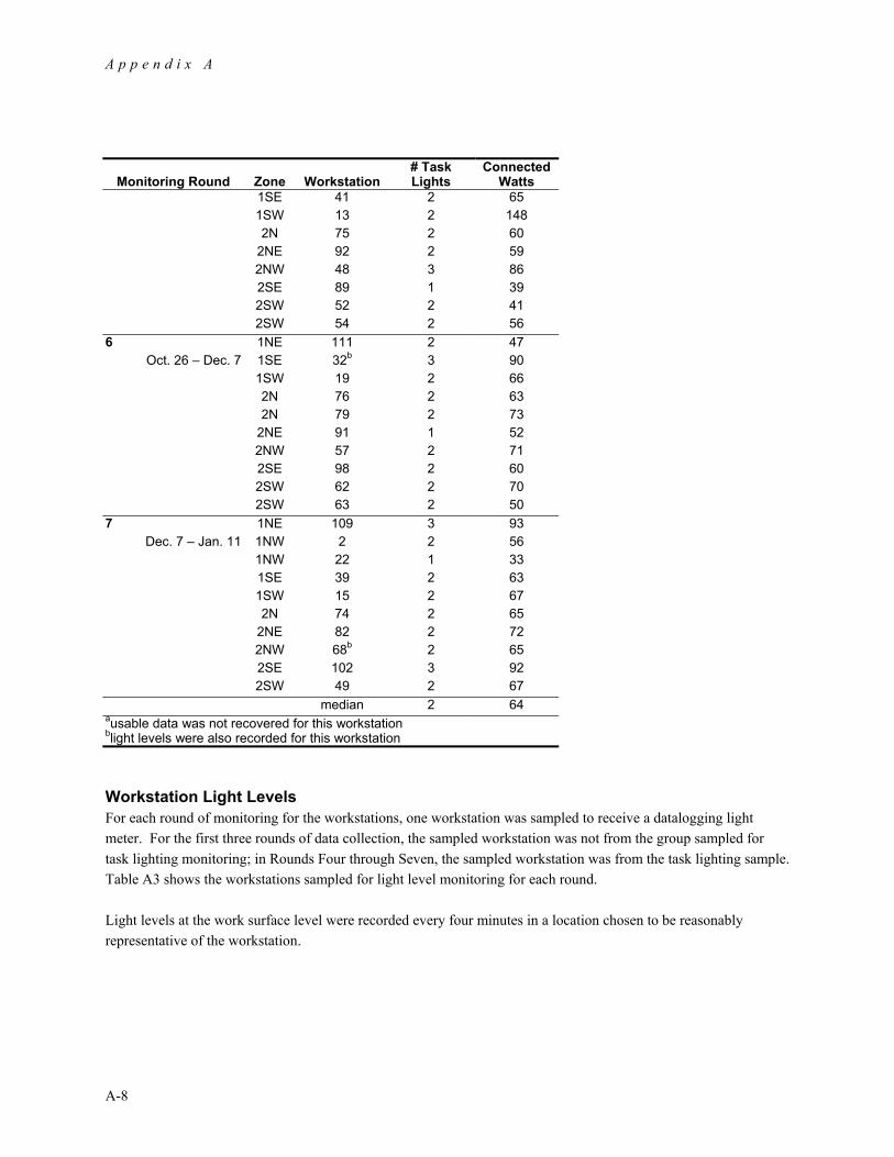
Workstation Task Lighting In addition to overhead ambient lighting, nearly all workstations in the building have built-in task lighting in the form of under-cabinet fluorescent lighting. In addition, some employees have table lamps and other task lighting. To assess the amount of task lighting at Hoffman, the following monitoring protocol was used for most (but not all) months during the monitoring period. Each month, ten workstations were randomly sampled to have task lighting monitored. The samples were drawn such that one workstation was sampled (without replacement) from each of nine defined zones on the first and second floors of the building. The zones were defined based on the floor and the compass quadrant of the zone (Figure A4). One zone was randomly chosen each month to receive the tenth data logger, and an additional workstation was sampled within that zone. Workstation lighting was monitored by segregating all task lights for a workstation on a single terminal strip and then plugging this terminal strip into an outlet equipped with a line splitter. The line splitter allowed the installation of a current transformer which was connected to a Brultech data logger which also measured line voltage to calculate lighting power consumption. Wattages were sampled and recorded hourly. Table A3 shows the stations that were monitored.

Second Floor

First FloorNorth

2SW

2NW

2N

2NE

2SE

1SW

1NW 1NE

1SE

Second Floor

First FloorNorthNorth

2SW

2NW

2N

2NE

2SE

1SW

1NW 1NE

1SE

Figure A4, Zones for workstation monitoring.

A p p e n d i x A

A-7

Table A3, Workstation task lighting monitoring.

Monitoring Round Zone Workstation # Task Lights

ConnectedWatts

1 1NE 36 1 30 May 19 – June 21 1SE 35 2 74

1SW 8 2 60 1SW 16 2 72 2N 70 2 57 2N 77 2 59 2NE 67 3 90 2NE 83 1 50 2SE 87a 2 69 2SW 51 3 102

1SW 9b light level monitoring only 2 1NE 110 2 60

June 21 – July 19 1NW 6 1 21 1SE 44 2 62 1SW 14 2 55 2N 72 2 62 2N 81a 2 63 2NE 95 1 35 2NW 47 4 99 2SE 100 3 91 2SW 65 2 72

2N 75b light level monitoring only 3 1NE 37 3 106

July 19 – August 31 1SE 31 2 74 1SW 7 3 90 1SW 17 3 94 2N 69 3 94 2N 71 3 99 2NE 84 2 57 2NW 59a 4 136 2SE 90 1 33 2SW 53 2 60

2SW 62b light level monitoring only 4 1NE 108 na na

August 31 – Sept. 28 1NW 21 na 56 1SE 29 na na 1SW 4 na na 2N 73 na na 2NE 96b na 40 2NW 55 na na 2SE 86 na na 2SE 97 na na 2SW 64 na na

5 1NE 38b 2 62 Sept. 28 – Oct. 26 1NW 3 2 85

A p p e n d i x A

A-8

Monitoring Round Zone Workstation # Task Lights

ConnectedWatts

1SE 41 2 65 1SW 13 2 148 2N 75 2 60 2NE 92 2 59 2NW 48 3 86 2SE 89 1 39 2SW 52 2 41 2SW 54 2 56

6 1NE 111 2 47 Oct. 26 – Dec. 7 1SE 32b 3 90

1SW 19 2 66 2N 76 2 63 2N 79 2 73 2NE 91 1 52 2NW 57 2 71 2SE 98 2 60 2SW 62 2 70 2SW 63 2 50

7 1NE 109 3 93 Dec. 7 – Jan. 11 1NW 2 2 56

1NW 22 1 33 1SE 39 2 63 1SW 15 2 67 2N 74 2 65 2NE 82 2 72 2NW 68b 2 65 2SE 102 3 92 2SW 49 2 67 median 2 64

ausable data was not recovered for this workstation blight levels were also recorded for this workstation

Workstation Light Levels For each round of monitoring for the workstations, one workstation was sampled to receive a datalogging light meter. For the first three rounds of data collection, the sampled workstation was not from the group sampled for task lighting monitoring; in Rounds Four through Seven, the sampled workstation was from the task lighting sample. Table A3 shows the workstations sampled for light level monitoring for each round. Light levels at the work surface level were recorded every four minutes in a location chosen to be reasonably representative of the workstation.

A p p e n d i x A

A-9

Chiller Analysis

Demand under Design Conditions To estimate the average chiller demand at design conditions, we regressed afternoon (12- 4pm) chiller demand against dry bulb and dew point air temperature for all non-holiday weekdays with usable data. As the scatterplot matrix in Figure A5 shows, average chiller demand during this period is well-correlated with dry-bulb temperature, and somewhat less so with dewpoint temperature.

The regression results are as follows:

chiller demand (kW) = 1.94*dry-bulb temperature + 0.36*dewpoint temperature – 115 (n=50, r2=0.85)

When the 1% design conditions for Appleton (89oF dry-bulb and 68 oF dewpoint temperature) are applied to the regression equation above, an estimated chiller electrical load of 82 ± 4 kW is obtained (error bands are 90 percent confidence intervals). This corresponds to 62 ± 3 percent of full output for the installed 102-ton chiller, or 63 tons. A similar analysis based on the maximum daily chiller demand during this period (instead of the average demand), yields a maximum chiller load of 91 ± 4 kW, corresponding to about 70 tons of capacity.

Average dry-bulbtemperature [F]

0

50

100

40 60 80 100

Average chillerdemand (kW)

20 40 60 80

Average dewpointtemperature [F]

Figure A5, Afternoon (12-4pm) chiller electrical demand versus dry-bulb and dewpoint temperatures.

A p p e n d i x A

A-10

Annual Chiller Electricity Use

To estimate annual chiller electricity use under average conditions, we used the Princeton Scorekeeping Method (PRISM.5 This model fits daily chiller electricity use to cooling degree days, with the best-fit reference temperature for cooling degree-days also calculated from the model. The model is:

chiller kWh per day = α + βc hc (τc )

where,

α = non-weather sensitive (or base) kWh per day

βc = kWh per cooling degree day

hc = cooling degree days per day from base temperature τ, which are calculated from daily average outdoor temperatures (Tavg) as:

Hc = max(Tavg - τc,0)

τc = base temperature for calculating cooling degree days

We used weather data for Green Bay, Wisconsin, because long-term normals were available for this station. The long-term averages were based on the 20-year period from 1980 through 1999.

We fit the model separately for weekday and weekend usage, since the cooling setpoint differs between these two periods. The results are shown in Table A4, and indicate about 66,000 kWh annually for chiller electricity consumption.

Table A4, Chiller weather correction model results.

Period n α βc τc r2

Weather normalized

annual average usage Weight

Weekdays 115 9.9 ± 11.8 34.9 ± 1.2 50.8 ± 0.6 0.94 220.0 kWh/day 5/7

Weekends 44 2.2 ± 10.9 21.6 ± 2.9 56.0 ± 1.7 0.83 86.96 kWh/day 2/7

Combined 182.0 kWh/day

66,427 kWh/year

Note: error bars are standard errors.

5Advanced, Version 1.0 was used. See Fels, M. 1986. “PRISM: An Introduction,” Energy and Buildings, Vol. 9, #1-2, pp. 5-18.

A p p e n d i x A

A-11

Fan Systems The Hoffman Building utilizes three supply fan systems AC1, AC2, and AC3. There are also three return air systems VA1, VA2, and VA3. Motor horsepower for each system is shown in Table A5 below.

Table A5, Ventilation supply and return fan horsepower.

Fan System Supply Fan Hp Return Fan Hp Total

AC1/VA1 20 3 23

AC2/VA2 20 5 25

AC3/VA3 25 5 30

Each fan system is equipped with a variable speed drive (VSD). Figure A6 shows the percent-speed data for a typical cooling-season and a non-cooling season day. What is noteworthy about the data is that fan system AC1/VA1 (and AC2/VA2 during the cooling system) run at about 100 percent speed during the night. This phenomenon was consistent throughout the monitoring period. (Subsequent to review of a draft version of this report, this was later traced by the building operations subcontractor to a programming error in the EMS system.)

0 2 4 6 8 10 12 14 16 18 20 22 240

20

40

60

80

100 AC1AC2

AC3

Hour

Air Handler Percent Speed (July 30, 2001)

0 2 4 6 8 10 12 14 16 18 20 22 240

20

40

60

80

100

Hour

AC1AC2

AC3

Air Handler Percent Speed (October 11, 2001)

0 2 4 6 8 10 12 14 16 18 20 22 240

20

40

60

80

100 AC1AC2

AC3

Hour


0 2 4 6 8 10 12 14 16 18 20 22 240

20

40

60

80

100 AC1AC2

AC3

Hour


0 2 4 6 8 10 12 14 16 18 20 22 240

20

40

60

80

100

Hour

AC1AC2

AC3


0 2 4 6 8 10 12 14 16 18 20 22 240

20

40

60

80

100

Hour

AC1AC2

AC3


Figure A6, Air handler fan speeds for two typical days.

A p p e n d i x A

A-12

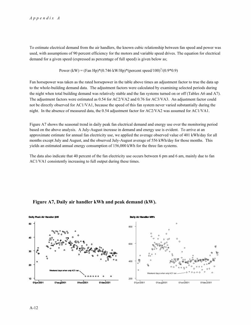
To estimate electrical demand from the air handlers, the known cubic relationship between fan speed and power was used, with assumptions of 90 percent efficiency for the motors and variable speed drives. The equation for electrical demand for a given speed (expressed as percentage of full speed) is given below as;

Power (kW) = (Fan Hp)*(0.746 kW/Hp)*(percent speed/100)3/(0.9*0.9) Fan horsepower was taken as the rated horsepower in the table above times an adjustment factor to true the data up to the whole-building demand data. The adjustment factors were calculated by examining selected periods during the night when total building demand was relatively stable and the fan systems turned on or off (Tables A6 and A7). The adjustment factors were estimated as 0.54 for AC2/VA2 and 0.76 for AC3/VA3. An adjustment factor could not be directly observed for AC1/VA1, because the speed of this fan system never varied substantially during the night. In the absence of measured data, the 0.54 adjustment factor for AC2/VA2 was assumed for AC1/VA1.

Figure A7 shows the seasonal trend in daily peak fan electrical demand and energy use over the monitoring period based on the above analysis. A July-August increase in demand and energy use is evident. To arrive at an approximate estimate for annual fan electricity use, we applied the average observed value of 401 kWh/day for all months except July and August, and the observed July-August average of 556 kWh/day for those months. This yields an estimated annual energy consumption of 156,000 kWh for the three fan systems.

The data also indicate that 40 percent of the fan electricity use occurs between 6 pm and 6 am, mainly due to fan AC1/VA1 consistently increasing to full output during these times.

01jun2001 01aug2001 01oct2001 01dec200110

20

30

40

50

Daily Peak Air Handler (kW

Weekend days when only AC1 ran

01jun2001 01aug2001 01oct2001 01dec2001200

400

600

800

Daily Air Handler kWh


01jun2001 01aug2001 01oct2001 01dec200110

20

30

40

50



01jun2001 01aug2001 01oct2001 01dec200110

20

30

40

50



01jun2001 01aug2001 01oct2001 01dec2001200

400

600

800



01jun2001 01aug2001 01oct2001 01dec2001200

400

600

800


01jun2001 01aug2001 01oct2001 01dec2001200

400

600

800



Figure A7, Daily air handler kWh and peak demand (kW).

A p p e n d i x A

A-13

Table A7, Data used to estimate demand for AC3/VA3.

Fan Speed (%)

Date HourAC1/VA1

AC2/VA2

AC3/VA3

Building kW

08/12/01 96.9 100.0 0.0 39.5597.1 100.0 0.0 39.36

2 96.9 100.0 0.0 39.7497.3 100.0 0.0 39.3697.1 100.0 81.4 48.3896.6 100.0 81.9 50.69

3 96.8 100.0 81.9 50.8896.7 100.0 81.8 51.2696.8 100.0 82.0 50.88

08/13/01 1 98.1 100.0 0.0 39.7497.9 100.0 0.0 39.5597.7 100.0 0.0 39.9498.2 100.0 0.0 39.55

2 98.3 100.0 0.0 39.9497.9 100.0 85.0 52.4297.6 100.0 81.6 51.0797.9 100.0 82.3 51.65

3 98.0 100.0 82.4 51.4698.5 100.0 82.4 51.2698.1 100.0 82.8 51.8498.4 100.0 83.0 51.26

4 98.0 100.0 83.3 51.6508/19/01 98.2 100.0 0.0 40.51

1 98.3 100.0 0.0 40.5198.4 100.0 0.0 40.9098.3 100.0 0.0 41.0998.4 100.0 0.0 40.51

2 98.1 100.0 87.0 47.6297.9 100.0 85.8 53.9597.8 100.0 86.1 53.7698.4 100.0 86.6 53.76

3 98.6 100.0 86.8 53.5798.1 100.0 86.9 54.14

08/21/01 97.4 100.0 0.0 41.4797.7 100.0 0.0 41.28

3 97.7 100.0 0.0 41.2898.0 100.0 0.0 41.2897.8 100.0 83.9 54.9198.3 100.0 84.6 53.76

4 97.6 100.0 85.4 53.9597.6 100.0 85.5 54.3497.4 100.0 85.7 58.18

Table A6, Data used to estimate demand for AC2/VA2.

Fan Speed (%)

Date Hour AC1/VA1

AC2/VA2

AC3/VA3

Building kW

09/09/01 99.1 0.0 0.0 27.07 99.1 0.0 0.0 26.88 1 99.6 0.0 0.0 26.88 99.3 0.0 0.0 27.26 99.1 100.0 0.0 28.42 98.6 100.0 0.0 39.94 2 99.1 100.0 0.0 39.94 98.8 100.0 0.0 39.55 98.4 100.0 0.0 39.74 98.9 100.0 0.0 39.36

09/16/01 98.8 0.0 86.1 46.46 21 98.8 0.0 86.2 46.27 98.6 0.0 86.1 46.66 99.3 0.0 86.1 46.46 99.1 0.0 86.2 46.66 22 98.4 100.0 85.9 48.77 99.0 100.0 85.9 58.94 98.3 100.0 85.9 58.37 98.9 100.0 85.9 59.52 23 98.4 100.0 86.0 58.75

A p p e n d i x A

A-14

Weather Normalized Total Electric and Gas Energy We also analyzed monthly utility billing records from January through December 2001, using the PRISM model described previously in this appendix under “Annual Chiller Electricity Use.” The monthly billing data shown in Table A8, electricity and natural gas use per day were regressed on cooling and heating degree days per day, respectively. The results are shown in Table A9 below.

Table A8, Hoffman building utility billing history.

Electricity

Peak Demand

Billing Period Natural

Gas

Energy

Overall 9am - 9pm

From To (therms) (kWh) (kW) (kW)

01/03/01 01/31/01 2,159 33,120 84 84

01/31/01 03/03/01 2,167 37,200 84 84

03/03/01 04/02/01 1,902 32,640 81.6 81.6

04/02/01 05/01/01 1,398 33,360 163.2 163.2

05/01/01 06/01/01 1,046 40,320 177.6 177.6

06/01/01 06/29/01 669 41,760 175.2 175.2

06/29/01 07/31/01 707 63,120 199.2 196.8

07/31/01 08/28/01 616 56,880 201.6 192

08/28/01 09/27/01 797 47,280 182.4 180

09/27/01 10/29/01 1,045 39,360 153.6 153.6

10/29/01 12/03/01 1,303 42,000 139.2 139.2

12/03/01 01/03/02 1,848 38,160 129.6 129.6

Total 15,657 505,200

Table A9, Weather correction model results.

n α βh,c τh,c r2 Weather normalized

annual average usage

Natural Gas 12 22.4 ± 3.8 1.19 ± 0.16 62.1 ± 5.7 0.94 16,480 ± 570 kWh

Electricity 12 1,166 ± 37 49.5 ± 12.3 55.5 ± 3.7 0.94 500,600 ± 9,400 therms

Note: error bars are standard errors.

A p p e n d i x A

A-15

Carbon Dioxide Monitoring

Indoor carbon dioxide was monitored from September through December. Five Telaire 7001 portable CO2 sensors were used for the monitoring. These were connected to Hobo data loggers to record CO2 concentration at 30-minute intervals. The Hobo data loggers also recorded temperature and relative humidity. The approximate location of the four sensors on the first and second floor of the building is shown in Figure A8. The fifth sensor was located in the small office area in the basement.

Second Floor

First FloorBasement Office Area

CO2 sensor location

Second Floor

First FloorBasement Office AreaBasement Office Area

CO2 sensor locationCO2 sensor location

Figure A8, Location of CO2 sensors.

A p p e n d i x A

A-16

B-1

Appendix B — Survey of Employees

Hoffman Building Office Environment Survey

Please indicate your response to the questions below by marking the appropriate box.

Lighting Conditions 1. Thinking about the last 12 months, how would you rate the amount of light at your workstation? (n=70)

Much too dim (3%) A little too dim (13%) About right (73%) A little too bright (8%) Much too bright (3%)

2. Most of the workstations at the Hoffman building include fluorescent task lights—and people sometimes add other task lights to their workstation. Thinking about the last 12 months, about how many hours per day did you use task lights at your workstation? (n=71)

Never (38%) Less than 1 hour per day (20%) More than 1 hour, but less than 4 hours per day (4%) More than 4 hours per day (38%)

A p p e n d i x B

B-2

3. Glare from windows or lights can sometimes be a problem. How often does glare bother you when… (n=70)

…you’re working at your computer?

All of the time (3%) Most of the time (4%) Sometimes (30%) Seldom (24%) Never (39%)

…you’re reading at your workstation?


4. Thinking about the last 12 months, how would you rate the temperature and humidity at your workstation in the summer and winter?

Temperature Summer Winter (n=69) (n=67) Much too cool (6%) (7%)

A little too cool (27%) (16%) About right (51%) (54%)

A little too warm (13%) (21%) Much too warm (3%) (2%)

Humidity Summer Winter (n=65) (n=65)

Much too humid (0%) (0%) A little too humid (8%) (0%)

About right (86%) (69%) A little too dry (6%) (26%) Much too dry (0%) (5%)

A p p e n d i x B

B-3

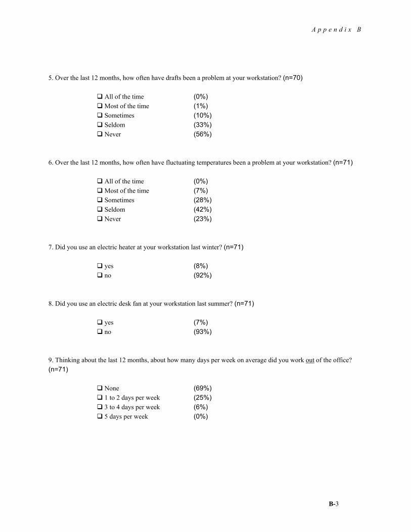
5. Over the last 12 months, how often have drafts been a problem at your workstation? (n=70)


6. Over the last 12 months, how often have fluctuating temperatures been a problem at your workstation? (n=71)


7. Did you use an electric heater at your workstation last winter? (n=71)

yes (8%) no (92%)

8. Did you use an electric desk fan at your workstation last summer? (n=71)

yes (7%) no (93%)

9. Thinking about the last 12 months, about how many days per week on average did you work out of the office? (n=71)

None (69%) 1 to 2 days per week (25%) 3 to 4 days per week (6%) 5 days per week (0%)

A p p e n d i x B

B-4

10. Again, thinking about the last 12 months, about how many hours per day did you spend at your workstation on average when you were working in the office? (n=71)

Less than 2 hours per day (1%) 2 to 3 hours per day (9%) 4 to 6 hours per day (28%) More than 6 hours per day (62%)

Summing It All Up 11. Overall, over the last 12 months, how would you rate the quality of light at your workstation? (n=71)

Very poor (0%) Poor (8%) Average (21%) Good (43%) Very Good (28%)

12. Overall, over the last 12 months, how would you rate the quality of your workstation environment in terms of temperature and humidity? (n=70)

Very poor (1%) Poor (11%) Average (36%) Good (40%) Very Good (11%)

Please Tell Us About Yourself (For Statistical Purposes Only): 13. Your gender: (n=71)

Female (41%) Male (59%)

A p p e n d i x B

B-5

14. Your age: (n=71)

Under 20 (0%) 20 to 29 (21%) 30 to 39 (38%) 40 to 49 (30%) 50 to 59 (10%) 60+ (1%)

15. Do you work full time or part time? (n=71)

Full time (93%) Part time (7%)

16. How long have you occupied your current workstation? (n=71)

Less than 6 months (24%) Six to 11 months (44%) 12 months or more (32%)

ENERGY CENTEROF WISCONSIN

595 Science Drive

Madison, WI 53711

Phone: 608.238.4601

Fax: 608.238.8733

Email: [email protected]

www.ecw.org

Printed on Plainfield Plus,

a recycled chlorine-free stock

containing 20% post-consumer waste.

performance monitoring of a daylit commercial office

Documents