PERFORMANCE MEASUREMENT TOOLS FOR HIGH-

LEVEL PARALLEL PROGRAMMING LANGUAGES

by

R. Bruce Irvin

A dissertation submitted in partial fulfillment of the requirements

for the degree of

Doctor of Philosophy

(Computer Sciences)

at the

UNIVERSITY OF WISCONSIN - MADISON

1995

i

ACKNOWLEDGMENTS

My years in Madison have been exciting, to say the least, and I never could have survived them

without the superb and consistent help of others. Bart Miller deserves my highest gratitude for

many years of advice, guidance, and support. Bart has shown a dedication that is both extraordi-

nary and admirable. If I only remember a fraction of what Bart has taught me, I will have learned

more than I ever imagined I could.

My committee members (Jim Goodman, Sangtae Kim, Jim Larus, and Miron Livny) each

offered their time and effort to review, criticize, and improve my work. I thank them for helping to

make the process worthwhile and for lending their insights and expertise.

Many other professors have helped me in small and large ways. In particular, I thank Chuck

Dyer for helping to admit me into the department, Bob Mayo for supporting me during my first

year, and Scott Baden of UCSD for reviewing my thesis proposal and providing many stimulating

discussions over Ethiopian lunches at the library mall.

I believe that the CS department’s staff is unequaled in its talent and dedication. In particular,

I thank Thea Sklenar for processing all those travel reimbursements (and letting me win at rball)

and Lorene Webber for acting as the cosmic glue of our department. I thank Paul Beebe, Mitali

Lebeck, Jim Luttinen, David Parter and all the rest of the Computer Systems Lab for taking our

computing environment from the 80s to the 90s without waiting for the 00s. I also thank Glenn

Ecklund for keeping the CM-5 chugging along.

I’ll never forget the IPS-2 and Paradyn projects, and their members will forever deserve my

admiration. Thank you Jeff Hollingsworth, Jon Cargille, Krishna Kunchithapadam, Mark Cal-

laghan, Karen Karavanic, Tia Newhall, Ari Tamches, Christopher Maguire, Mike McMenemy,

Joerg Micheel, Chi-Ting Lam, Marcelo Goncalves, Oscar Naim, Mark McAuliffe, and Suhui

ii

Chiang. Special thanks to Jeff and Mark for distinguished service as officemates.

My friends have been understanding sounding boards, moral supporters, providers of lodging,

and stellar geeks. In particular, I’d like to thank David McKeown, John Wood, Cliff Michalski,

Greg Wilson, Rob Netzer, Joann Ordille, Dave Cohrs, Lambert Wixson, Paul Carnine, Rick Ras-

mussen, Renee Miller, and Alvy Lebeck.

I thank Gary Kelley of Informix and Neal Wyse of Sequent for early support and encourage-

ment of my work. I thank Jerry Yan, Ken Stevens and the rest of the NASA Ames crew for later

support and encouragement. I thank NASA and the HPCC program for my graduate research fel-

lowship.

I owe great debts to all those who provided parallel programs for the measurements presented

in this dissertation. Thank you Dennis Jespersen, Leo Dagum, Bruce Davis, Brad Richards, Rob-

ert Schumacher, Jens Christoph Maetzig, and Vincent Ervin.

Finally, there is a group of people for whom I reserve special gratitude. Jill, Emma, my par-

ents, and my family have helped me immeasurably. This work is dedicated to them.

iii

ABSTRACT

Users of high-level parallel programming languages require accurate performance information

that is relevant to their source code. Furthermore, when their programs experience performance

problems at the lowest levels of their hardware and software systems, programmers need to be

able to peel back layers of abstraction to examine low-level problems while maintaining refer-

ences to the high-level source code that ultimately caused the problem. This dissertation

addresses the problems associated with providing useful performance data to users of high-level

parallel programming languages. In particular it describes techniques for providing source-level

performance data to programmers, for mapping performance data among multiple layers of

abstraction, and for providing data-oriented views of performance.

We present NV, a model for the explanation of performance information for high-level paral-

lel language programs. In NV, a level of abstraction includes a collection of nouns (code and data

objects), verbs (activities), and performance information measured for the nouns and verbs. Per-

formance information is mapped from level to level to maintain relationships between low-level

activities and high-level code, even when such relationships are implicit.

The NV model has helped us to implement support for performance measurement of high-

level parallel language applications in two performance measurement tools (ParaMap and Para-

dyn). We describe the design and implementation of these tools and show how they provide per-

formance information for CM Fortran programmers.

Finally, we present results of measurement studies in which we have used ParaMap and Para-

dyn to improve the performance of a variety of real CM Fortran applications running on CM-5

parallel computers. In each case, we found that overall performance trends could be observed at

iv

the source code level and that both data views and code views of performance were useful. We

found that some performance problems could not be explained at the source code level. In these

cases, we used the performance tools to examine lower levels of abstraction to find performance

problems. We found that low-level information was most useful when related to source-level code

structures and (especially) data structures. Finally, we made relatively small changes to the appli-

cations’ source code to achieve substantial performance improvements.

v

Table of Contents

Acknowledgments i

Abstract iii

Chapter 1. Introduction 1

1.1 Motivation . . . . . . . . . . . . . . . . . . . . . . . . . . . . . . . . . . . . . . . . . . . . . . . . . . . . . . . . . . 1

1.2 Summary of Results . . . . . . . . . . . . . . . . . . . . . . . . . . . . . . . . . . . . . . . . . . . . . . . . . . . 3

1.3 Organization of Dissertation . . . . . . . . . . . . . . . . . . . . . . . . . . . . . . . . . . . . . . . . . . . . 5

Chapter 2. Related Work 6

2.1 Tools that are Independent of Programming Model . . . . . . . . . . . . . . . . . . . . . . . . . . 6

2.2 Tools for Specific Programming Models . . . . . . . . . . . . . . . . . . . . . . . . . . . . . . . . . . . 8

2.3 Data Views of Performance . . . . . . . . . . . . . . . . . . . . . . . . . . . . . . . . . . . . . . . . . . . . 12

2.4 Complementary Techniques . . . . . . . . . . . . . . . . . . . . . . . . . . . . . . . . . . . . . . . . . . . 13

2.5 Summary . . . . . . . . . . . . . . . . . . . . . . . . . . . . . . . . . . . . . . . . . . . . . . . . . . . . . . . . . . 14

Chapter 3. The NV Model 17

3.1 Nouns and Verbs . . . . . . . . . . . . . . . . . . . . . . . . . . . . . . . . . . . . . . . . . . . . . . . . . . . . 18

3.2 Levels of Abstraction . . . . . . . . . . . . . . . . . . . . . . . . . . . . . . . . . . . . . . . . . . . . . . . . . 21

3.3 Application of NV Model to Actual Programming Models . . . . . . . . . . . . . . . . . . . 24

Chapter 4. Mapping 27

4.1 The Challenges of Mapping Performance Data . . . . . . . . . . . . . . . . . . . . . . . . . . . . . 27

4.2 Types of Mapping Information . . . . . . . . . . . . . . . . . . . . . . . . . . . . . . . . . . . . . . . . . 29

4.3 Static Mapping Information . . . . . . . . . . . . . . . . . . . . . . . . . . . . . . . . . . . . . . . . . . . . 30

4.4 Dynamic Mapping Information . . . . . . . . . . . . . . . . . . . . . . . . . . . . . . . . . . . . . . . . . 32

vi

4.4.1 The Use of Dynamic Instrumentation for Dynamic Mapping . . . . . . . . . . . . . 33

4.5 The Set of Active Sentences . . . . . . . . . . . . . . . . . . . . . . . . . . . . . . . . . . . . . . . . . . . 34

4.5.1 Description of the SAS . . . . . . . . . . . . . . . . . . . . . . . . . . . . . . . . . . . . . . . . . . . 35

4.5.2 Performance Questions . . . . . . . . . . . . . . . . . . . . . . . . . . . . . . . . . . . . . . . . . . . 37

4.5.3 Distributed Memory . . . . . . . . . . . . . . . . . . . . . . . . . . . . . . . . . . . . . . . . . . . . . 38

4.6 Limitations of the SAS Approach . . . . . . . . . . . . . . . . . . . . . . . . . . . . . . . . . . . . . . . 39

4.7 Summary . . . . . . . . . . . . . . . . . . . . . . . . . . . . . . . . . . . . . . . . . . . . . . . . . . . . . . . . . . 40

Chapter 5. ParaMap: Initial Experiments with NV 41

5.1 The ParaMap Tool . . . . . . . . . . . . . . . . . . . . . . . . . . . . . . . . . . . . . . . . . . . . . . . . . . . 42

5.2 Implementation . . . . . . . . . . . . . . . . . . . . . . . . . . . . . . . . . . . . . . . . . . . . . . . . . . . . . 43

5.3 Measurement Results . . . . . . . . . . . . . . . . . . . . . . . . . . . . . . . . . . . . . . . . . . . . . . . . . 46

5.3.1 Simple Example . . . . . . . . . . . . . . . . . . . . . . . . . . . . . . . . . . . . . . . . . . . . . . . . 47

5.3.2 Dual Reciprocity Boundary Element Method . . . . . . . . . . . . . . . . . . . . . . . . . . 50

5.4 Summary . . . . . . . . . . . . . . . . . . . . . . . . . . . . . . . . . . . . . . . . . . . . . . . . . . . . . . . . . . 55

Chapter 6. The NV Model with Dynamic Instrumentation 57

6.1 The Paradyn Parallel Program Performance Measurement Tool . . . . . . . . . . . . . . . . 58

6.1.1 Resources and Metrics . . . . . . . . . . . . . . . . . . . . . . . . . . . . . . . . . . . . . . . . . . . 59

6.1.2 System Structure . . . . . . . . . . . . . . . . . . . . . . . . . . . . . . . . . . . . . . . . . . . . . . . . 61

6.2 Source-level Performance Data in Paradyn . . . . . . . . . . . . . . . . . . . . . . . . . . . . . . . . 63

6.3 Mapping of Performance Data Between Levels of Abstraction . . . . . . . . . . . . . . . . 64

6.4 CM Fortran-Specific Resources and Metrics . . . . . . . . . . . . . . . . . . . . . . . . . . . . . . . 66

6.4.1 Performance Data for Parallel Arrays . . . . . . . . . . . . . . . . . . . . . . . . . . . . . . . . 66

6.4.2 Parallel Code Constructs . . . . . . . . . . . . . . . . . . . . . . . . . . . . . . . . . . . . . . . . . . 68

vii

6.4.3 CMRTS Metrics . . . . . . . . . . . . . . . . . . . . . . . . . . . . . . . . . . . . . . . . . . . . . . . . 69

6.5 Measurement of CM Fortran Programs . . . . . . . . . . . . . . . . . . . . . . . . . . . . . . . . . . . 69

6.6 Vibration Analysis (Bow) . . . . . . . . . . . . . . . . . . . . . . . . . . . . . . . . . . . . . . . . . . . . . 71

6.6.1 Peaceman-Rachford PDE Solver (Peace) . . . . . . . . . . . . . . . . . . . . . . . . . . . . . 78

6.6.2 Particle Simulation (PSICM) . . . . . . . . . . . . . . . . . . . . . . . . . . . . . . . . . . . . . . 83

6.7 Summary . . . . . . . . . . . . . . . . . . . . . . . . . . . . . . . . . . . . . . . . . . . . . . . . . . . . . . . . . . 89

Chapter 7. Conclusions 91

7.1 Summary . . . . . . . . . . . . . . . . . . . . . . . . . . . . . . . . . . . . . . . . . . . . . . . . . . . . . . . . . . 91

7.2 Future Work . . . . . . . . . . . . . . . . . . . . . . . . . . . . . . . . . . . . . . . . . . . . . . . . . . . . . . . . 93

Chapter 8. Bibliography 98

1

1. Introduction

1.1 Motivation

Proponents of high-level parallel programming languages promise to make programmers’ lives

easier. Parallel languages offer portable, concise notations for specifying parallel programs, and

their compilers automatically map programs onto complex parallel machines. Furthermore, paral-

lel languages free programmers from the difficult, error-prone, and sometimes ineffective task of

specifying parallel computations explicitly. Unfortunately, high-level parallel programming

languages cannot guarantee high performance because compilers are often unable to effectively

map programs to target hardware. Programmers often must add pragmas or rewrite code to

accommodate compilers, particular architectures, operating systems, or data sets.

Performance measurement tools can give programmers insight for performance tuning, but

past performance measurement techniques have not been effectively applied to programs written

in high-level parallel programming languages. Tools have either been designed for specific pro-

gramming languages and incorporated a narrow view of program performance, or have been

designed for low-level programming and presented information that was unusable by a high-level

programmer.

There are several problems associated with building performance tools for high-level parallel

programming languages. First and most important, performance tools must converse with pro-

grammers using the terms of the source code language. More specifically, users must be able to

measure performance metrics for each important control construct in their language.

2

Second, performance tools must account for implicit activity. We define implicit activity as

extra activity that is inserted by a compiler to maintain the illusion of a programming model for a

particular hardware platform. This problem is best illustrated by the observation that as program-

mers use more and more abstract programming languages they understand less and less of the

detailed execution of their programs. In general, programmers should leave as many hardware-

specific details to the compiler as possible, but we have observed that applications can perform

poorly because their high-level characteristics are not effectively processed by the compiler and

result in unnecessarily large amounts of implicit activity. Of course, better compilers and standard

hardware may eventually ease this problem, but until then, performance tools must measure

implicit activity and relate it to the source code constructs that ultimately required it.

Third, performance tools for high-level parallel programming languages must include data-

oriented (in addition to control-oriented) views of performance. Many of today’s parallel pro-

gramming languages use data structures to express parallelism, and users must effectively decom-

pose their data structures across distributed memories to achieve good performance. Performance

tools must therefore relate performance measurements to distributed data-structures so that users

may make effective data distribution decisions.

Finally, performance tools for high-level parallel programming languages must allow pro-

grammers to study performance at multiple levels of abstraction. When implicit activity limits an

application’s performance, we cannot always fully understand an application’s performance by

simply knowing which source level control or data structures caused bottlenecks. Again, due to

the nature of abstraction, high-level information alone may be too vague. Therefore, to aggres-

sively find and fix performance problems we must look beneath the highest layers. But as we

noted above, simply providing raw performance data in terms of processors, caches, and commu-

3

nication is overwhelming and confusing. Instead, performance tools must constrain and identify

low-level information with source code level information.

1.2 Summary of Results

This dissertation presents new methods for collecting and presenting performance information for

programs written in high-level parallel programming languages and shows that the methods are

very effective in practice. Our methods are based on the Noun-Verb (NV) model, an informal

framework for reporting performance information for programs built on multiple levels of

abstraction. We show how we have used the model to develop performance tools for a data-paral-

lel Fortran dialect. These tools present both code and data views of performance, account for

implicit activity, and allow users to peel back layers of abstraction when necessary. We demon-

strate the effectiveness of the tools by measuring and improving execution times of several real

applications.

The NV model allows us to organize complex, layered programming systems. With NV, we

associate performance information with performance-critical control and data structures at the

source code level, we map implicit activity to the source code level, and we allow users to peel

back layers of abstraction when performance problems lie beneath the source code level.

The NV model describes an application program as a set of levels of abstraction. Each level

corresponds to a layer of software or hardware in the actual application program. Each level con-

tains a set of nouns and a set of verbs. Nouns are the structural elements of each level and verbs

are the actions taken by the nouns or performed on the nouns. Nouns and verbs from one level of

abstraction are related to nouns and verbs from other levels of abstraction with mappings. A map-

ping expresses the notion that high-level language constructs are implemented with low-level

software and hardware.

4

The NV model allows us to measure performance information at low levels (where it is easy

to measure) and map it to performance information at the source code level (where it is easy to

understand). Furthermore, the model is independent of programming system. We have used the

model to study several parallel programming language classes, and we have used the model to

implement performance tools for one specific language, CM Fortran.

Aside from the NV model, this dissertation describes several other important contributions.

We demonstrate that performance data should be related to data structures and show how it can be

done. Today’s most successful parallel programming systems exploit parallelism in data and it is

therefore important for performance tools to correlate performance information to parallel data

structures. We describe how data structures are represented in the NV model and demonstrate per-

formance measurements for parallel arrays in Fortran.

We describe how compilers can communicate static mapping information to performance

tools. We describe a language-independent interface to static mapping information that we have

implemented in the Paradyn performance measurement system. The interface allows compilers to

describe the nouns, verbs, and levels of abstraction in a given program as well as the mappings

between nouns and verbs at different levels.

But static mapping information is not sufficient to fully represent relationships between levels

of abstraction. Today’s programming systems may defer mapping decisions until hardware con-

figurations are known and many systems reassign data structures to processors to optimize com-

putation or communication load. Therefore, we describe and evaluate a language independent

mechanism for communicating dynamic mapping information to performance tools.

Finally, we tie together all of our ideas by demonstrating their use in practice. Throughout this

dissertation, we examine several real applications donated by today’s users of parallel computers.

5

By measuring and significantly improving these applications, we aim to not only help today’s

users to improve their programs’ execution times, but also to show tomorrow’s programmers that

high-level parallel programming languages can be used to effectively and efficiently utilize very

complex parallel computers.

1.3 Organization of Dissertation

The remainder of this dissertation is divided into 6 chapters. After covering relevant previous

work, we present and evaluate the NV model in the middle five chapters. We then summarize and

outline future research directions.

Chapter 3 describes the NV model in detail. We use several examples taken from data-parallel

Fortran to illustrate important ideas in the model.

Chapter 4 describes basic techniques for mapping. We present simple examples of static map-

ping and discuss the complex problem of dynamic mapping.

Chapter 5 describes an initial implementation of NV for the CM Fortran data-parallel pro-

gramming language. It describes measurements of a dual-reciprocity boundary element code and

presents evidence that performance tools based on the NV model can lead to substantial improve-

ments in application performance.

Chapter 6 discusses the use of dynamic performance measurement techniques. We discuss the

Paradyn performance tool, our enhancements for the collection and use of mapping information,

and the support of CM Fortran. The chapter concludes with three measurement experiments in

which we find and fix substantial performance problems in each application.

Finally, Chapter 7 summarizes the contributions of this thesis and outlines goals for future

research.

6

2. Related Work

Prior research in parallel program performance tools has addressed many issues related to the

measurement of high-level parallel language programs. Most of the implemented performance

measurement systems provide performance data relevant to either the lowest levels of abstraction

(e.g., messages, locks, basic block counts) or the highest levels of a specific programming model.

These two approaches correspond to the goals of building tools that can be used with many pro-

gramming models and tools that are designed for use with a single programming model. In this

chapter we discuss how previous tools have supported users of parallel programming languages.

We conclude that although each system addressed some of the issues described in Chapter 1, no

single system has conversed with users in terms of source code, accounted for implicit activity,

supported the study of performance at multiple levels of abstraction, and provided data views of

performance.

2.1 Tools that are Independent of Programming Model

Most performance measurement tools for sequential and parallel systems measure execution char-

acteristics that are independent of programming model. For the purpose of this discussion, I

divide such general tools into two categories — system monitoring tools and general program

monitoring tools.

System monitoring tools provide performance information about the hardware and system

software at the base of a parallel or distributed system. For example, hardware monitors measure

bus activity, cache activity, memory activity, instruction types, vector performance, I/O sub-

7

systems, or networks [1,2,3]. Operating systems monitors usually monitor processor utilization,

scheduling, virtual memory activity, I/O activity, or system calls [4]. Although these tools can be

used while programs of any language execute on a system, their measurements cannot easily be

related to individual constructs of a particular language. Therefore, it is difficult to use system

monitoring tools alone to fully understand the performance of a parallel or distributed program.

Hardware and operating system monitors are most useful for tuning the performance of a system

itself or for supplementing program performance measurement tools [22].

General program monitoring tools use a variety of techniques to measure common-denomina-

tor events. Common-denominator events include procedure calls [2,44], basic blocks [34,47,53],

runtime libraries [44], synchronization points [36], and the operating system kernel [45]. The

information gathered from the probes is summarized into metrics, analyzed, displayed, and some-

times mapped back to source code via the program’s symbolic debugging information

[14,19,46,54,59,70].

General program monitoring tools can provide extensive views of performance, but they can

be confusing for users of high-level parallel programming languages. Such tools can usually pro-

vide execution statistics for every process, library, function, basic block, statement, or instruction

in an application. Since such measurements are independent of source language, many languages

can be studied. However, the user is responsible for understanding how the source constructs of

their programming language map to the primitive events measured by the tool.

For example, visualizations of low-level send/receive communication may confuse program-

mers who use data-parallel languages. Several general program monitoring tools include mea-

surements of message send and receive events. However, such a view of performance may

confuse a programmer who has been using higher level constructs such as data-parallel array

8

notations. Such a programmer may not understand the concepts associated with sending and

receiving messages, much less understand which code or data objects are responsible for which

messages.

2.2 Tools for Specific Programming Models

Several performance measurement tools have been designed for specific languages or program-

ming environments. Language-specific tools are able to use knowledge of the programming

model to reduce overall measurement costs and give detailed performance feedback. Such tools

provide information about specific language constructs or data types that is not visible to more

general low-level tools. However, language-specific tools have not generally provided any infor-

mation about lower levels of abstraction and have usually ignored the effects of implicit activity.

Language-specific tools are not generally applicable to programs written in other languages.

The tools include analyses and displays that may be generally useful, but because the tools are

bound to specific data collection mechanisms and language terms, it is difficult to re-apply their

techniques for new languages. One of the goals of the NV model is to identify concepts and tech-

niques that can be applied across parallel programming languages.

Several excellent performance tools have been designed for use with data-parallel program-

ming languages. The Connection Machine Prism environment is a debugging and performance

measurement tool for C* and CMFortran programs [60]. It monitors subroutine and runtime sys-

tem events and provides profiles of CPU time and various types of message communication. A

similar tool, called MPPE, is provided on MasPar machines for programs written in MasPar For-

tran [41]. Each tool allows the user to see which lines of code are primarily responsible for pro-

gram activity. Some implicit system-level information is provided, usually in terms of total time

spent in library routines. The work described in this dissertation extends these ideas by relating

9

such measurements to parallel data structures (the primary source of parallelism in data-parallel

languages) and extends performance measurements to the parallel node level of abstraction.

The PerfSim performance prediction tool [66] takes a different approach to measuring CM

Fortran applications. PerfSim executes the sequential part of a CM Fortran program and estimates

the running times of the parallel parts by replacing the CM Fortran runtime system with a perfor-

mance prediction library. The tool can be used to quickly estimate the running time of an applica-

tion. However, it does not address the problem of identifying the causes of performance problems.

Furthermore, it assumes that the costs of parallel library routines can be accurately estimated and

that sequential activity can be cheaply executed. My experience (related in Chapters 4, 5, and 6)

suggests that the costs of parallel executions can be unpredictable and that sequential activity can

unfortunately create significant performance problems.

The Cray Research product ATExpert analyzes do loops of autotasked Fortran programs on

Cray Research Y-MP and C90 computers [69]. The tool measures the implicit costs associated

with the parallelization of loops and orders the costs for each loop. Each type of cost is related to

a strategy for improving the performance of loops, and therefore the tool is able to suggest spe-

cific improvements for each loop. My work extends ATExpert’s techniques by generalizing the

concepts behind implicit cost measurements and by providing tools that directly measure implicit

costs for other types of programming constructs.

Two recent performance measurement systems use extensive compiler information to provide

detailed performance information for data-parallel Fortran dialects. The D system provides per-

formance feedback for Fortran D applications [1]. It integrates the Fortran 77D compiler with the

Pablo performance measurement environment. The result is an editor that annotates source code

lines with performance information such as computation time and message statistics. The D sys-

10

tem also performs sophisticated analysis of static and dynamic trace data to provide detailed, lan-

guage-dependent information such as identification of loop-carried cross-processor dependencies.

The Cray Research product MPP Apprentice [68] uses compiler-generated instrumentation and

cost estimates to time and count language-level events for the myriad programming models of the

Cray T3D. By timing and counting events, MPP Apprentice achieves scalability. Through inte-

gration with the Cray Research compilers, MPP Apprentice provides information that is relevant

to parallel source code.

The integration of compilers with performance tools achieved by the D system and MPP

Apprentice is crucial in obtaining detailed, code-specific information. In the future, further inte-

gration will likely enable the measurement of data-specific information as well. The NV model

and the program information interfaces described in Chapters 5 and 6 suggest how this might be

accomplished in a way that is independent of specific compilers.

Several performance tools have been designed for parallel functional languages. A static anal-

ysis tool designed for the Id functional language allows the user to view the potential parallelism

for Id programs [3]. The tool analyzes the structure of a program’s dataflow graph to determine

the maximum and average widths of the graph as well as the length of the critical path through the

static dataflow graph. Such tools are useful with functional languages, in which program depen-

dencies can be determined before execution. Runtime profiling tools that account for unique exe-

cution activities such as lazy evaluation have been developed for other functional languages such

as Haskell [55]. The ParVis tool presents program performance visualizations that are unique to

the Multilisp parallel programming language [38]. Multilisp is a dialect of LISP that includes

functions, called futures, that return their values asynchronously. ParVis allows the user to view

parallelism and waiting in terms of the activities of futures.

11

All of the functional language performance tools are excellent examples of tools that converse

with users in the terms of the source code language. They present parallelism and synchronization

in terms of functions, evaluations, and futures. However, compilers for functional languages often

generate significant amounts of implicit low-level activity (e.g. garbage collection) to produce

executable binaries for traditional hardware systems; therefore, it is especially important for per-

formance tools for functional languages to measure and present information about implicit low-

level activity.

A growing number of performance tools are designed for parallel object-oriented languages.

Most notably, TAU is the official performance analysis system for the pC++ programming lan-

guage [48]. It uses source-level event traces to display parallel performance information in terms

of class methods and uses a rich program information database [6] to relate events to source code.

The Projections tool presents language-specific performance information about the distributed

object-oriented programming language CHARM (or CHARE kernel) [27]. A Projections user can

display message traffic over time and differentiate message information by message type. The

programming environment for the object-oriented language COOL allows the user to specify

object characteristics that affect performance and reliability [58]. The characteristics are grouped

into versions, called adaptations, that can be used to dynamically adapt an application to varying

runtime environments.

Each of the tools for parallel object-oriented languages relates performance measurements to

code, but none of the tools relates performance to parallel data. Because the data objects are the

primary source of parallelism in such languages, it is crucial to relate computation and communi-

cation to objects. Some of the tools (especially Projections) measure implicit low-level activity

(message communication) and classify it according to the purpose of the activity, but in general,

12

these tools have concentrated on source-level information.

A few performance measurement systems have been designed for parallel logic languages.

The Gauge performance measurement tool [28] presents high-level information for programs

written in PCN [13]. Gauge collects various metrics on per-procedure and per-process bases and

displays the metrics in a color-coded matrix. The tool also computes metrics that are specific to

guarded case statements, called implications. The per-implication metrics include the number of

times an implication was considered, the number of times an implication succeeded or failed, and

the number of times an implication blocked waiting for input values.

2.3 Data Views of Performance

A few previous tools have supported data-oriented views of performance. In particular, memory

trace tools such as Cprof [35] and MemSpy[17] have successfully related cache hits and misses to

data structures in sequential C and Fortran programs. Several algorithm animation and visualiza-

tion tools have been developed as part of sequential object-oriented programming systems [18,

31, 12]. Each of these object-oriented systems draws a representation of an object hierarchy and

then animates the view with execution information such as recordings of object activations and

method invocations.

Performance views of parallel data structures have been more limited, but recent work in the

area of performance visualization [30, 25] has focused on drawing representations of vectors and

matrices, annotating these representations with data layouts, and animating the views with traces

of computation and communication events. Our work differs from these efforts in that we have

not attempted to visualize and animate the actual data structures (a task that becomes considerably

more difficult with increasing scale and dimension). Instead, we have concentrated on collecting

dynamic mapping information for parallel data structures and mapping node-level performance

13

measurements of explicit and implicit activities to the data structures.

2.4 Complementary Techniques

Research in event mapping tools and in debugging optimized code offer results and methodolo-

gies that are related to the performance measurement of high-level parallel languages. Event map-

ping tools allow programmers to build up abstractions by describing relationships between

records in an event trace file, and debuggers for optimized code attempt to accurately represent

the state of program execution across abstraction levels after an optimizing compiler has obscured

low-level execution details.

Event mapping is a hybrid approach to system monitoring that is capable of bridging the gap

between general measurement tools and language-specific tools. Event mapping tools generally

collect low-level events and map them to higher levels of abstraction for analysis by a user. The

user is responsible for describing how low-level events are to be combined and identified as high-

level events and is responsible for analyzing the high-level events for the desired performance

information. This approach provides maximum flexibility in handling program performance

information.

Event definitions may be provided in terms of grammars [5], relations [61], or constructs of a

special language [29,52]. An event mapping system compiles the definitions and automatically

recognizes the defined high-level events within streams of low-level events. Generally, event

mapping tools support multiple levels of abstraction, enabling the user to study program perfor-

mance from multiple views.

Event mapping is useful for any tool that must present information at multiple levels of

abstraction. However, the general problem addressed by existing tools —mapping all event

streams to all types of performance information —is a difficult problem. We feel that the regular-

14

ity of events generated by high-level language compilers and runtime systems allows us to map

aggregate performance information (such as metrics and summations) without the immediate

need of the more general (and more costly) event mapping methods.

Performance measurement of programs written in high-level languages bears some resem-

blance to the problem of debugging optimized code [20]. In the latter problem, a symbolic debug-

ger must present a view of an optimized program that is consistent with the original source code

hiding the effects of optimizations that reordered statements, eliminated variables, or otherwise

altered the steps of a computation. The resultant code may not have a direct mapping to the origi-

nal source code and may not even be representable in the source language. Most work in this field

has focused on identifying variables containing values consistent with the source code (variable

currentness) and on providing the values of such variables [8,20,71]. Some work has investigated

ways of displaying the execution of optimized code in terms of the source code [7].

Performance measurement of parallel programs written in high-level languages is fundamen-

tally simpler than the debugging of optimized code because performance measurement tools need

not reconstruct the instantaneous state of a computation. A symbolic debugger must be able to

stop the execution of a program at any instruction, identify the corresponding location in the

source code, and provide access to variables in the original program. A performance measurement

tool, on the other hand, is generally concerned with the cumulative activity of program elements

(code constructs and data objects). Performance measurement tools must identify the program

elements that are active at a given point but rarely need access to the values of variables.

2.5 Summary

The NV model augments earlier work in performance tools for parallel programming languages.

It uses and builds on many of the individual techniques used by general measurement tools, lan-

15

guage-specific tools, and event-mapping tools.

General performance tools offer a variety of data collection techniques, from specialized hard-

ware [9,64,67], to library instrumentation [37,40,44], to source code instrumentation [54], to

dynamic rewriting of code in execution [24,43]. The NV model does not require any particular

method of collection and the tools described in this dissertation employ a variety of data collec-

tion techniques pioneered by other tools. However, various techniques for dynamic mapping of

performance data are more practically implemented with dynamic instrumentation techniques. In

Chapter 4, we demonstrate the space and time savings of making mapping decisions dynamically.

Language-specific performance tools have demonstrated several individual measurement

techniques that we can use in performance tools based on the NV model. Data-parallel language

tools have shown how to provide control (code) views of performance [1,41,60,68], and we adopt

their techniques for attaching performance data to code displays. Object-oriented language tools

offer natural hierarchical structures for organizing noun data [48] and demonstrate techniques for

interpreting compiler output for mapping purposes. The standardization of compiler-generated

mapping data is still an unsolved problem, but these systems demonstrate its potential and we

push these techniques further in this dissertation.

Event mapping tools introduced the notions of abstraction layers and querying of performance

data. We adopt and expand the concept of abstraction layer by showing that they can be used

dynamically to constrain low-level measurements without the inherent overhead of event-map-

ping techniques. We also define a new form of performance data query that allows a restricted

subset of multi-level performance data to be collected efficiently.

The remainder of this dissertation combines and expands on the techniques provided by these

related systems. It offers techniques for representing performance information at multiple layers

16

of abstraction, for accounting for implicit activity, for automatically mapping performance data

between layers, and for providing data views of performance.

17

3. The NV Model

To identify performance characteristics that are common across programming models, we have

developed a framework within which we can discuss performance characteristics of programs

written in these programming models. This section describes the Noun-Verb (NV) model for par-

allel program performance explanation. In the NV model, nouns are the structural elements of a

particular program, and verbs are the actions taken by the nouns or performed on the nouns.1

The collection of nouns and verbs of a particular software or hardware layer defines a level of

abstraction. Nouns and verbs from one level of abstraction are related to nouns and verbs from

other levels of abstraction with mappings. A mapping expresses how high-level language con-

structs are implemented by low-level software and hardware. With mappings, performance infor-

mation collected at arbitrary levels of abstraction can be related to language level nouns and

verbs. A mapping may be static, meaning that it is determined before runtime, or dynamic, mean-

ing that it is determined at runtime and possibly changes over the course of program execution.

Besides providing a framework for comparing performance characteristics across program-

ming models, the NV model helps explain the performance characteristics of any particular pro-

gramming language. By directly accounting for both implicitly and explicitly mapped verbs, the

NV model provides a more complete view of program performance. Furthermore, the model can

be used as a guide to creating performance measurement tools.

1. An alternate terminology could be objects and methods. However, we feel that these terms have beenoverused, so we have chosen nouns and verbs.

18

In this chapter, we describe the NV model using the data-parallel language CM Fortran [65] as

our example language. CM Fortran (and its implementation on CM-5 computers) is representative

of many high-level parallel programming languages, including HPF [21]. The NV model, how-

ever, is applicable to many other parallel programming models.

3.1 Nouns and Verbs

A noun is any program element for which performance measurements can be made, and averb is

any potential action that might be taken by a noun or performed on a noun. We will use the exam-

ple CM Fortran program in Figure1 to describe some of the nouns and verbs of the CM Fortran

language. The example program declares two multi-dimensional arrays (line 3), initializes all ele-

ments of arrayA with a parallel assignment statement (line 5), assigns values to a subsection of

arrayA (line 7), computes the sum of the array (line 8), and computes a function of the upper left

quadrant of arrayA and assigns it to arrayB (line 9).

First, we identify the nouns in the example program. CM Fortran nouns include programs

(line 1), subroutines, FORALL loops, arrays (A andB on line 3), and statements (lines 5, and 7-9).

Verbs in CM Fortran include statementexecution (lines 5-10), arrayassignment (lines 5, 7, and 9)

andreduction (line 8), subroutineexecution, and fileIO.

With some programming languages, naming particular nouns can be difficult, and we may

need to generate unique names for them. For example, many languages (such as Lisp and C) do

not explicitly identify dynamically created data objects, and we might name such nouns in a vari-

ety of ways.

• We may name them after the control structure within which they were allocated. For example,

(retval foo) might name the list returned by functionfoo() in a Lisp program.

• For cases in which we want to differentiate between various calls to a memory allocation rou-

19

tine, we may add the names of functions that are currently on the dynamic call stack. For

example, (retval (foo bar)) might indicate the list returned by function foo() when called by

function bar(). This is similar to the scheme used in the Cprof memory profiler [35].

• We could name objects by the memory location at which they are allocated. For example,

noun:5000 might represent the data object allocated at memory location 5000.

• We could give unique global or local names to dynamically allocated nouns. For example

noun:56 might indicate the 56th object allocated during program execution.

• We could ask the programmer to supply a name. For example, we could ask C programmers to

supply an extra argument to calls to the memory allocator malloc().

• In object-oriented languages such as C++, we may name dynamically created instances of a

class using the class name and an identifier. For example, Queue:34 might indicate the 34th

instance of class Queue.

• We may use a combination of these schemes to produce a compound name.

Code structures such as loops, iterators, switches, and simple statements also can be difficult

to name because languages and compilers rarely give them explicit names. We might name such

nouns in several different ways.

• The simplest (and most common) approach is to name code structures after the location at

which they are defined. For example foo.f/doloop:53 might identify the do loop that begins at

line 53 of the Fortran program contained in the file foo.f.

• We may ask the programmer to insert compiler pragmas into their code to name particular

control structures. For example, the programmer could give a name such as innerLoop to a

particularly important loop.

• In some languages, programmers can create control structures dynamically, and we can name

20

them with one of the schemes proposed above for dynamic data objects.

Each of these approaches has advantages and disadvantages, and no single approach is supe-

rior in all cases. Therefore, we must choose the best scheme for the particular languages that we

measure.

It is often useful to group nouns into sets, trees, graphs, or other structures. Noun grouping

simplifies searching the set of nouns, organizes performance information for efficient access, and

reflects program structure. For example, the set of statements within a subroutine can be grouped

together to indicate the natural structure of a body of code. Groupings may be based on noun

types, names, or performance characteristics.

1 PROGRAM EXAMPLE2 PARAMETER (N=1000)3 INTEGER A(N+1,N+1), B(N,N), ASUM45 A = 06 DO K = 1,107 FORALL (I = 2:N+1, J = 2:N+1) A(J,I) = K*(I+J)8 ASUM = SUM(A)9 FORALL (I = 1:N/2, J = 1:N/2) B(J,I) = A(J,I) + A(J+1,I+1)10 END DO11 END

Figure 1: Example CM Fortran Program

A particular execution instance of the program construct described by a verb is called a sen-

tence. A sentence consists of a verb, a set of participating nouns, and a cost. The cost of a sentence

may be measured in terms of such resources as time, memory, or channel bandwidth. Finally, per-

formance information consists of the aggregated costs measured from the execution of a collec-

tion of sentences. For example, performance information for array A might include measurements

of the assignments of lines 5, 7, and 9, and the reduction on line 8. Performance information for

array B, however, would include only measurements of the assignment on line 9.

21

The method of expression of a verb is either explicit, meaning that the verb was directly

requested by the programmer through the use of a program language construct, or implicit, mean-

ing that the programmer did not explicitly request the verb but that it occurred to maintain the

semantics of the computational model. Examples of implicit verbs include page faults, cache

misses, and process initialization.

3.2 Levels of Abstraction

High-level language programs are usually built on several levels of abstraction, including the

source code language, runtime libraries, operating system, and hardware. In well constructed sys-

tems, each level is self-contained; levels interact through well-defined interfaces. It is possible to

measure performance at any level, but measurements may not be useful if they are not related to

constructs that are understood by the programmer. In the NV model, each level of abstraction for

which performance may be measured is represented by a distinct set of nouns and verbs. Further-

more, nouns and verbs of one level may be mapped to nouns and verbs in other levels.

For CM-5 systems, a CM Fortran program is compiled into a sequential program and a set of

node routines. The sequential program executes on the CM-5 Control Processor and makes calls

to the parallel node routines and to parallel system routines through the CM Runtime System

(CMRTS). The CMRTS creates arrays, maps arrays to processors, implements CM Fortran intrin-

sic functions (e.g., SUM, MAX, MIN, SHIFT, and ROTATE), and coordinates the processor

nodes. Each parallel CM Fortran array is divided into subgrids, and each subgrid is assigned to a

separate node. Each node is responsible for computations involving its local array subgrids; if

array data from non-local subgrids are needed, then the non-local data must be transferred before

computation can proceed.

22

Figure 2 shows the division of the CM-5 system into three levels of abstraction for the NV

model. The highest level, called the CMF level, contains the nouns and verbs from the CM For-

tran language, as discussed in Section 3.1. The middle level is the RTS level. RTS level nouns

include all of the arrays allocated during the course of execution. This set of arrays includes all of

the arrays found in the CMF level as well as all arrays generated by the compiler for holding inter-

mediate values during the evaluation of complex expressions. Verbs of the RTS level include

array manipulations such as Shift, Rotate, Get, Put, and Copy. The lowest level of abstraction is

the node level. Node level nouns include all of the processor nodes. Node level verbs include

Compute, Wait, Broadcast Communication, and Point-to-Point Communication.

A mapping relates nouns (verbs) from one level of abstraction to nouns (verbs) of another

level. A mapping may be top-down or bottom-up. For example, a top-down mapping from arrays

to nodes might relate a particular array (or subsection of an array) to a particular set of processor

nodes. A bottom-up mapping from node routines to code lines might relate CPU time recorded for

a particular node routine to the CM Fortran statement from which it was compiled.

NV mappings are either static or dynamic. Static mappings are independent of time or context.

For example, the mapping between node level object routines and CMF level statements is a static

mapping that is determined at compile time. Dynamic mappings are time-varying relationships.

For example, CM Fortran arrays are mapped to processor nodes when they are allocated, so map-

pings between nodes and array subregions must be recorded at runtime.

Verb mappings are either explicit or implicit. An explicit mapping indicates that a high- level

verb is directly implemented by a lower level verb. For example, a SUM reduction (line 8 of

Figure 1) might be implemented by low-level addition operations, and the mapping from CMF

level SUM operations to node level additions is therefore explicit. Implicit mappings indicate that

23

a lower-level verb helps to maintain the semantics of a higher-level verb. For example, a SUM

reduction is implemented on a CM-5 system with partial reductions on each processor node and a

final reduction of the partial results using the CM-5 broadcast network. The parallelism and

broadcast communication created by such a reduction is implicit because neither is specified

directly by the CMF level SUM statement. Therefore, the NV mapping from CMF level SUM

operations to creation of parallelism and broadcast communication is an implicit mapping.

Figure 2: CM-5 Execution of a CM Fortran Program. Shaded areas indicate usercode. The labels along the right edge indicate the levels of abstraction in the NV

representation of CM Fortran.

CMFLevel

RTSLevel

NodeLevel

Control Processor

System

CM RunTime

CM Node

Array SubGrids

RTSRoutines

Sequential

CMF

Object Code

CM−5 System

CMFObject

Code

CMF

Source

CodeCM Node

24

3.3 Application of NV Model to Actual Programming Models

Hundreds of parallel programming languages have been proposed and several have been imple-

mented and even distributed for general use. We find that the NV model is useful for describing

the performance aspects of particular languages as well as entire classes of languages. In this sec-

tion, we briefly describe how nouns, verbs, levels of abstraction, and mappings could be used with

a variety of example languages.

Jade [33] is a task-parallel language that uses accesses to shared data structures to synchronize

tasks. A Jade withonly block is a coarse-grained task that specifies which shared objects it

needs to access before executing. The Jade runtime system ensures that a withonly block has the

appropriate access before allowing the block to execute. The NV representation of Jade models

withonly blocks and shared data objects as nouns and accesses to shared data objects as verbs.

The execution of a withonly block would explicitly map to the execution of the statements

within the block and accesses of the shared memory objects would implicitly map to time spent

waiting for the objects.

SISAL [42] is a parallel single-assignment language that has achieved performance compara-

ble to Fortran on several applications. A SISAL programmer creates functional loops that expose

code to parallel optimization techniques so that independent loops may be automatically sched-

uled on parallel processors. Nouns in a SISAL program include functions, loops, and expressions.

As with any functional language, the primary verb in SISAL is evaluation. Lower-level implic-

itly-mapped verbs include the scheduling and synchronization of the parallel loop iterations.

Portable runtime systems [39,62] are not normally considered to be languages, but from the

performance measurement point of view they share many characteristics with more traditional

languages. A portable runtime system implements a particular level of abstraction and may itself

25

be composed of multiple levels. For example, PVM uses a daemon on each workstation to set up

connections and route messages. Therefore, PVM operations potentially map to multiple daemon

operations, each of which affects the performance of a PVM operation.

Parallel programming libraries [63] and class libraries [32] are also not normally considered to

be languages, but (as with portable runtime systems) we can nevertheless measure and explain

their performance with the aid of the NV Model. Each such library defines its own classes of

nouns and verbs. For example, LPARX defines the concepts of Regions, Grids, and XARRAYs. A

region is an abstract object representing an index space, a grid is a uniform dynamic array instan-

tiated over a region, and an XARRAY is a dynamic array of aggregate data objects, usually grids,

distributed over processors. In NV, we represent each of these concepts as a different type of

noun, and maintain mappings to indicate which grid is contained on which processors. LPARX

supports various activities (such as region partitioning, region growing, and XARRAY allocation)

and each corresponds to a verb in NV.

An algorithm is the ultimate high-level notation for a problem solution, and we can use NV to

help explain the performance of algorithms. Classes of algorithms usually manipulate common

data structures with common primitive actions. For example, graph algorithms generally specify

various ways of traversing the nodes and arcs of a graph, and matrix algorithms specify various

methods for manipulating the rows, columns, and elements of a matrix. In NV we represent the

basic elements of an algorithm as nouns (graphs, nodes, arcs, matrices, rows, columns, elements),

and we represent primitive operations as verbs (traverse, visit, mark, add, delete, transpose, move,

copy).

Algorithmic representations of problem solutions generally assume a known cost for all oper-

ations. For example, a graph algorithm analysis may assume a fixed cost for visiting, marking,

26

and deleting tree nodes. However, in an implementation, the actual costs may vary due to unpre-

dictable, implicit, low-level activities such as synchronization locking, communication, and file I/

O. By maintaining mappings from such low-level, implementation-dependent activities to the

high-level structures of an algorithm, we can better evaluate the validity of “known cost” assump-

tions and better evaluate the performance analyses of algorithms.

27

4. Mapping

A primary problem in the performance measurement of high-level parallel programming

languages is to map low-level events to high-level programming constructs. This chapter dis-

cusses important aspects of this problem and presents three methods with which performance

tools can map performance data and provide accurate performance information to programmers.

In particular, we discuss static mapping, dynamic mapping, and a new technique that uses a data

structure called the set of active sentences. Because each of these methods requires cooperation

between compilers and performance tools, we describe the nature and amount of cooperation

required. The three mapping methods are orthogonal; we describe how they should be combined

in a complete tool. Although we concentrate on mapping upward through layers of abstraction,

our techniques are independent of mapping direction. In Chapters 5 and 6, we evaluate these

methods in actual performance tools.

4.1 The Challenges of Mapping Performance Data

When application programs are built on multiple layers of abstraction, performance tools must

consider how nouns and verbs of each layer relate to nouns and verbs of other layers. As we

described in Chapter 3, the mapping provides a way to represent the relations between abstraction

levels for nouns or verbs. Any performance information that is measured for a sentence is relevant

not only to itself, but also to all nouns or verbs to which it maps.

To build mappings, performance tools must collect mapping information; such information

can take many forms in real systems. Many compilers emit symbolic debugging information,

28

which allows programming tools to map memory addresses to source code lines and data struc-

tures. However, common symbolic debugging information seldom provides the complete set of

mapping data needed by performance tools. For example, a list of data structures used on each

line of code (which is useful for mapping execution activity to data structures) is typically not

available. Other mapping information is stored only in application data-structures during execu-

tion. For example, a run-time system may determine data-to-processor mappings at run time after

it has knowledge of available hardware resources; run-time systems usually keep this information

in the program’s address space. Traditionally, there has been no well-defined way for run-time

systems and application programming libraries to communicate mapping information to perfor-

mance tools.

Mappings can be one-to-one, one-to-many, many-to-one, and many-to-many, as shown in

Figure 3. This figure shows examples of each type of mapping. One-to-one mappings (shown in

Type of Mapping ExampleHow to assign low-level

costs to high-level structure

One-to-One Low-level message send Simplements high-levelreduction R.

Measurements of S areequivalent to measure-ments for R.

One-to-Many Low-level function Fimplements reductions R1,R2, ...

(1) Cost of F is split evenlyover all R, or(2) Merge all R into oneset and assign cost of F toentire set.

Many-to-One Low-level functions (F1,F2, ...) implement onesource line L.

First aggregate costs ofF1,F2,... then assign cost toline L.

Many-to-Many Many source code lines L1,L2, ... are implemented byan overlapping set of low-level functions F1, F2,...

First aggregate costs of F1,F2, ..., then treat as a one-to-many mapping to L1,L2, ...

Figure 3: Types of Upward Mappings

29

the first row of the table in Figure 3) are relatively simple to handle in a performance tool. Any

performance information measured for one sentence is associated with the one sentence to which

it maps. However, when a sentence maps to several other sentences (one-to-many, shown in the

second row), the correct assignment of performance data is more difficult. In this case, many tools

split the measured data equally across all sentences to which the measured sentence maps [1,60].

However, such splitting assumes an equal distribution of low-level work to high-level code. It is

often better to handle one-to-many mappings by merging the sentences to which the measured

sentence maps [26]. The latter technique (used by the tool discussed in Chapter 5) makes no

assumption about the distribution of performance data and helps to identify high-level program-

ming constructs whose implementations have been merged by an optimizing compiler. It also

avoids misleading the programmer with overly precise information.

Many-to-one and many-to-many mappings (shown in the third and fourth rows of Figure 3)

can be reduced to the two types of mappings described above. In each case, we aggregate (either

sum or average) the performance data for the low-level sentences and then treat the result as a

one-to-one or one-to-many mapping. We show examples of each of these cases in Chapters 5 and

6.

4.2 Types of Mapping Information

Mapping information may include noun and verb definitions as well as detailed descriptions of

how particular nouns and verbs map to other nouns and verbs. In this section we describe a

generic interface for communicating mapping information to performance tools. In following sec-

tions we describe how this information may be communicated from compilers to tools both prior

to application execution (static information) and during execution (dynamic information).

30

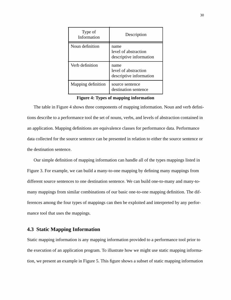
The table in Figure 4 shows three components of mapping information. Noun and verb defini-

tions describe to a performance tool the set of nouns, verbs, and levels of abstraction contained in

an application. Mapping definitions are equivalence classes for performance data. Performance

data collected for the source sentence can be presented in relation to either the source sentence or

the destination sentence.

Our simple definition of mapping information can handle all of the types mappings listed in

Figure 3. For example, we can build a many-to-one mapping by defining many mappings from

different source sentences to one destination sentence. We can build one-to-many and many-to-

many mappings from similar combinations of our basic one-to-one mapping definition. The dif-

ferences among the four types of mappings can then be exploited and interpreted by any perfor-

mance tool that uses the mappings.

4.3 Static Mapping Information

Static mapping information is any mapping information provided to a performance tool prior to

the execution of an application program. To illustrate how we might use static mapping informa-

tion, we present an example in Figure 5. This figure shows a subset of static mapping information

Type ofInformation

Description

Noun definition namelevel of abstractiondescriptive information

Verb definition namelevel of abstractiondescriptive information

Mapping definition source sentencedestination sentence

Figure 4: Types of mapping information

31

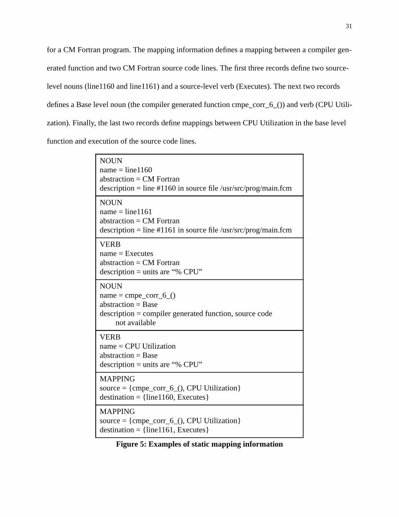
for a CM Fortran program. The mapping information defines a mapping between a compiler gen-

erated function and two CM Fortran source code lines. The first three records define two source-

level nouns (line1160 and line1161) and a source-level verb (Executes). The next two records

defines a Base level noun (the compiler generated function cmpe_corr_6_()) and verb (CPU Utili-

zation). Finally, the last two records define mappings between CPU Utilization in the base level

function and execution of the source code lines.

NOUNname = line1160abstraction = CM Fortrandescription = line #1160 in source file /usr/src/prog/main.fcm

NOUNname = line1161abstraction = CM Fortrandescription = line #1161 in source file /usr/src/prog/main.fcm

VERBname = Executesabstraction = CM Fortrandescription = units are “% CPU”

NOUNname = cmpe_corr_6_()abstraction = Basedescription = compiler generated function, source code

not available

VERBname = CPU Utilizationabstraction = Basedescription = units are “% CPU”

MAPPINGsource = {cmpe_corr_6_(), CPU Utilization}destination = {line1160, Executes}

MAPPINGsource = {cmpe_corr_6_(), CPU Utilization}destination = {line1161, Executes}

Figure 5: Examples of static mapping information

32

The mapping information indicates that the two statements on lines 1160 and 1161 of the

source code are implemented by a single low-level routine, and that if our performance measure-

ment tool can measure CPU Utilization for cmpe_corr_6_(), then it can present that information

as Execution of the corresponding source code lines. A performance tool may then split the exe-

cution costs between the two source code lines, merge the two lines into an inseparable unit, or

make other interpretations of the mappings.

Static mapping information may be kept in an application program’s executable image, in a

separate file, in an auxiliary database, or in some other static location. Regardless of its location,

the mapping information must be communicated to performance tools before they can use map-

pings for high-level abstractions.

The method of communicating static mapping information discussed in this section provides a

simple method with which compilers can describe important language-specific and program-spe-

cific information to performance tools. Because such information is defined statically, perfor-

mance tools can process it before or after the execution of the application program and avoid

competition for resources with the application program. However, static mapping information

usually cannot provide information about mappings that are determined during application execu-

tion.

4.4 Dynamic Mapping Information

Dynamic mapping information includes any mapping information that is generated during appli-

cation execution. It includes the same types of information as static mapping information (see

Figure 4), and differs with static mapping information only in that is communicated to perfor-

mance tools during program execution. For example, if an application dynamically allocates par-

allel data objects, then the application must dynamically communicate the definition of the

33

corresponding noun to the performance tool. If the application dynamically distributes the data

object across parallel processing nodes, then the application must dynamically define a mapping

between the object and processor nodes for the performance tool. The performance tool can use

the dynamic mapping information during or after run time to relate performance measurements to

abstract program constructs and activities.

In this section we discuss two important techniques for collecting dynamic mapping informa-

tion. The first uses dynamic instrumentation [24] to reduce the perturbation effects of collecting

dynamic mapping information, and the second uses a data structure called the Set of Active Sen-

tences to discover verb mappings that are otherwise difficult to detect.

4.4.1 The Use of Dynamic Instrumentation for Dynamic Mapping

A mapping point is any function, procedure, or line of code in an application where dynamic map-

pings may be constructed. For example, if we have a run-time system routine that allocates paral-

lel data objects and distributes them across processors, then the return point of the routine would

be defined as a mapping point; the mapping of data objects to processor nodes will be determined

just prior to that point. Our goal is to identify all such mapping points in an application, and

instrument them with code that reports mapping information to our performance tool. We can

instrument all such points by adding source code that calls our performance tool, or we can use

dynamic instrumentation to insert the mapping instrumentation at run time.

Dynamic instrumentation [24] is a technique whereby an external tool changes the binary

image of a running executable to collect performance data. The basic technique defines points at

which instrumentation can be inserted, predicates that guard the firing of the instrumentation

code, and primitives that implement counters and timers. Dynamic instrumentation provides an

advantage over traditional static techniques because it allows performance tools to instrument

34

only those points that are currently needed to provide performance data. Any point that does not

contain instrumentation does not cause any execution perturbations.

For dynamic mapping instrumentation, we can define a subset of points consisting of all those

points that generate mapping information. Typically, the subset is different for each language, or

programming library and includes the return points for all subroutines in which data structures are

allocated or in which distributions to parallel processors are determined. As an application exe-

cutes, a performance tool can either insert mapping instrumentation once at the beginning of exe-

cution and leave it in, or it can insert and delete mapping instrumentation throughout execution.

The latter technique reduces run-time perturbation but may miss mapping decisions or noun/verb

definitions.

4.5 The Set of Active Sentences

Some dynamic mapping information is difficult to determine by simply instrumenting mapping

points in an application. Verb mappings between layers of abstraction are often difficult to detect

because the implementation of one layer is usually hidden from other layers for software engi-

neering reasons. In this section we describe the Set of Active Sentences (SAS), a data structure

that allows us to dynamically map concurrent sentences between layers of abstraction. We

describe the SAS with an example taken from High Performance Fortran, describe the kinds of

questions that might be asked and answered with the SAS, and describe limitations of the SAS

approach.

1 ASUM = SUM(A)2 BMAX = MAXVAL(B)

Figure 6: Example HPF Code

35

4.5.1 Description of the SAS

The Set of Active Sentences (SAS) is a data structure that records the current execution state of

each level of abstraction similar to the way a procedure call stack keeps track of active func-

tions.Whenever a sentence at any level of abstraction becomes active, it adds itself to the SAS,

and when any sentence becomes inactive, it deletes itself from the SAS. Any two sentences con-

tained in the SAS concurrently are considered to dynamically map to one another.

For example, consider the example HPF code fragment in Figure 6. In this code, we are con-

cerned with the following problem: how to relate a low-level message to a high-level array reduc-

tion. The SUM reduction on line 1 and the MAXVAL reduction on line 2 of the code imply that

messages must be sent between processors on a distributed memory parallel computer. We

assume that each node of a parallel computer holds subsections of arrays A and B, and each node

reduces its subsections before sending its local results to other nodes to compute the global reduc-

tions. We assume that a performance tool can measure the low-level mechanisms for message

transfer (e.g., message send and receive routines), and can monitor the execution of the high-level

code (e.g., which line of code is active, which array is active, what reduction is being performed

on the array).

We want to answer such questions as:

• How many messages are sent for summations of A? For finding the MAXVAL of B?• How much time is spent sending messages for summations of A?

Although these questions are specific to data-parallel Fortran and in particular the HPF code in

Figure 6, they are representative of questions that we would like to ask for any language system

built on multiple layers of abstraction. In any such system, we want to explain low-level perfor-

mance measurements in terms of high-level programming constructs (and vice versa).

36

In the SAS approach to dynamic mapping, we defer the asking of performance questions until

run time, and then only measure those sentences that satisfy at least one performance question. As

explained above, the SAS keeps track of all sentences that are active at any level of abstraction.

Whenever any sentence becomes active, monitoring code notifies the SAS, and the SAS remem-

bers all such active sentences. When a low-level sentence is to be measured (whether by a

counter, timer, or any other means), monitoring code queries the SAS to determine what sentences

are currently active and thereby relates low-level sentences to active sentences at higher levels.

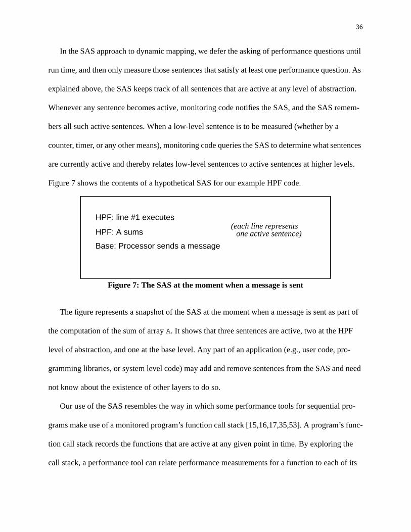
Figure 7 shows the contents of a hypothetical SAS for our example HPF code.

The figure represents a snapshot of the SAS at the moment when a message is sent as part of

the computation of the sum of array A. It shows that three sentences are active, two at the HPF

level of abstraction, and one at the base level. Any part of an application (e.g., user code, pro-

gramming libraries, or system level code) may add and remove sentences from the SAS and need

not know about the existence of other layers to do so.

Our use of the SAS resembles the way in which some performance tools for sequential pro-

grams make use of a monitored program’s function call stack [15,16,17,35,53]. A program’s func-

tion call stack records the functions that are active at any given point in time. By exploring the

call stack, a performance tool can relate performance measurements for a function to each of its

Figure 7: The SAS at the moment when a message is sent

HPF: line #1 executes

HPF: A sums

Base: Processor sends a message

(each line representsone active sentence)

37

ancestors in the program’s call graph. Users of such a performance tool can then understand how

function activity relates to the dynamic structure of their programs. The SAS, however, may

record any active sentence, regardless of whether the sentence could be discovered by examining

the call stack.

As defined, the SAS contains all sentences that are active. If we wish to reduce the size of the

SAS, we can also take advantage of run-time requests for performance information [43] to elimi-

nate uninteresting sentences from the SAS. For example, if we only ever request measurements

for array A, then the SAS may avoid keeping sentences that do not contain A.

4.5.2 Performance Questions

The SAS can also keep track of performance questions if they are asked using nouns and verbs as

described in Section 3.2. We define a performance question to be a vector of sentences. The mean-

ing of a performance question is that performance measurements (of resource utilization) should

be made only when all of the sentences of the question are active. Figure 8 shows a few of the

possible performance questions (and their meanings) for our example HPF code. Although the

questions in the figure consist of sentences that contain one noun and one verb, we can easily gen-

eralize questions to use more complex sentences without altering the operation of the SAS.

Performance Questions Meaning

{A Sum} Cost of summations of A?

{Processor_P Send} Cost of sends by processor P?

{A Sum}, {Processor_P Send} Cost of sends by P while A is beingsummed?

{? Sum}, {Processor_P Send} Cost of sends by P while anything isbeing summed?

Figure 8: Example performance questions

38

Monitoring code may use the SAS to answer the types of questions listed in Figure 8. Each

component of a performance question represents a predicate that must be satisfied before monitor-

ing code can measure CPU time, wall-clock time, channel bandwidth, or any other execution cost

for the question.

We can make the SAS more flexible by extending our definition of performance questions.

Currently, a performance question is satisfied only if the conjunction of its sentences are active.

We could extend the concept of performance questions to include boolean operators such as dis-

junction and negation. This would allow us to ask a much wider range of performance questions.

This extension incurs the added time to evaluate the more complex expressions.

4.5.3 Distributed Memory

We have defined the SAS to be a global data structure. If our target hardware systems support

shared global memory, then we can use globally shared memory to store the SAS. However, many

of today’s parallel systems do not use globally shared memory, and even for those that do, we may

not want to pay the synchronization cost of contention for such a globally shared data structure.

Fortunately, we can still use the SAS approach if we duplicate the SAS on each node of a parallel

computer, just as application code is duplicated for Single Program Multiple Data (SPMD) pro-

grams. Each individual SAS can operate independently of others as long performance questions

are not asked that require information from several SASs. For example, all of the performance

questions listed in Figure 8 can be answered without sharing any information between nodes.

Of course, some interesting performance questions can only be answered using information

about sentence activity on more than one node. For example, in a distributed database system, if a

server process performs disk reads on behalf of clients, then we may wish to measure server disk

reads that corrspond to a particular client or a particular query. The SAS information that is neces-

39

sary to answer such a performance question (server reads from disk, client query is active) would

be distributed between the SAS on the client and the SAS on the server. The client’s SAS and the

server’s SAS would need to communicate before the performance question could be answered. In

particular, the client’s SAS would need to send one sentence (i.e., client query is active) to the

server’s SAS whenever that sentence became active or inactive.

4.6 Limitations of the SAS Approach

The SAS approach to relating low-level performance information to high-level activities has at

least three limitations.

First, the SAS approach does not handle asynchronous activation of sentences. For example,

in a UNIX system we may want to measure kernel disk writes that occur on behalf of a particular

function in a user process. Figure 9 shows time-lines for a hypothetical UNIX process and kernel.

Figure 9: Asynchronous sentence activations and the SAS (time advances downward)

User Process Kernel

func() {..write();..

}

disk_write()disk_write()disk_write()

SAS

func()

kernel

executes

writes to disk

active

inactive

40

The user process makes a write() system call to the kernel and the kernel later writes the infor-

mation to disk. The actual writes to disk do not occur until later. The third column of the figure

shows how the SAS records each of these activities. As the figure shows, the SAS may not con-

tain both the function execution sentence and the kernel disk write sentence at the same time, and

therefore kernel disk writes on behalf of function func() could not be measured with the help of

the SAS alone.

Second, sentence activity notifications that are ignored by the SAS cause unnecessary execu-

tion costs. For our example code from Figure 6, if we only ask performance questions about array

A, then all activation notifications about array B are ignored by the SAS. But we must pay the run-

time cost of the notification. We could eliminate this cost by dynamically removing such notifica-

tions from the executing code [24].

Third, sentences are not ordered in performance questions. For our current definition of per-

formance question, the question “How many messages are sent for the summation of A?” is syn-

tactically equivalent to the question “How many summations of A occur when messages are

sent?” If we were to take advantage of sentence order in performance questions, then we could

distinguish between these two very different performance questions.

4.7 Summary

In this chapter, we have described the important problems of collecting, storing, communicating,

and using mapping information in performance tools for high-level parallel programming

languages. We have described a format and interface for static and dynamic mapping information,

and we have presented the Set of Active Sentences as a method for identifying complex dynamic

activity mappings. In the following chapters we present experiences taken from using these tech-

niques in various real program performance measurement tools.

41

5. ParaMap: InitialExperiments with NV

The NV model is not only a useful structure for understanding performance characteristics of

high-level parallel language programs, it also can be used as a guide for the design and implemen-

tation of performance measurement tools. For an initial evaluation of the NV model in this role

and to gain experience with mapping in an actual parallel language system, we built a perfor-

mance measurement tool for CM Fortran. The tool, called ParaMap, measures performance infor-

mation for nouns and verbs at three levels of abstraction (CM Fortran level, the Runtime System

level, and the Node level), maps performance information between levels, and provides both code

and data views of performance.

This chapter describes the design and implementation of ParaMap and demonstrates the tool

with actual CM Fortran applications. The tool is a post-mortem tool that uses a compact data for-

mat to record performance data. We describe ParaMap’s simple interface, its use of static and

dynamic mapping information, and its implementation on CM-5 systems.

Finally, we present case studies in which we have used ParaMap to measure and improve the

performance of a toy application and a real chemical engineering application. In these studies, we

find that high-level performance data (especially for CM Fortran parallel assignments and parallel

arrays), mapping between levels of abstraction, and data views of performance are all useful in

understanding and improving the execution characteristics of the applications.

42

5.1 The ParaMap Tool

The design of ParaMap follows the NV description of CM Fortran given in Chapter 3. Measured

nouns at the CMF level of abstraction include subroutines, statements, and arrays, while verbs

include array assignment and reduction, subroutine execution, and statement execution. At the

RTS level, ParaMap measures the cost of array manipulations such as Shift, Copy, and Move. At

the node level, ParaMap measures computation (CPU utilization), waiting, and broadcast commu-

nication. Point-to-point communication at the node level is difficult to measure directly on CM-5

computers, so we approximate it in ParaMap by measuring process time in node-level routines

that perform point-to-point communications.

ParaMap uses a simple interface to give users post mortem access to performance informa-

tion. The user constructs sentences from nouns and verbs and asks the tool for the measured cost

of the constructed sentences. Costs are provided in three formats: a count of the number of times

the sentence was recorded, the total time cost of the sentence, and a time plots showing the cost of

the sentence graphed over time. Each level of abstraction is separated in the interface; the current

level must be selected by the user. The user constructs sentences using only nouns and verbs at the

current level.

ParaMap uses static and dynamic mappings to compute the costs of high-level sentences.

When a user asks for the cost of a sentence, ParaMap will map the request to explicit computa-

tions in low-level compiler-generated functions (called PN code blocks) as well as implicit runt-

ime system activities such as shifting or broadcasting the array. If the user selects a sub-region of

the array, then ParaMap will only provide information from the processors on which the elements

of the selected subregion are stored.

43

ParaMap also uses mappings to implement contexts. A context is a set of nouns and verbs

selected by the user for the purpose of constraining performance information at lower levels. For

example, a ParaMap user may select an array A and the verb Reduction at the CMF level and ask

the tool to create a context C. Then, when the user peels back layers of abstraction by moving to

the RTS or node level, ParaMap uses C to constrain the set of nouns and verbs that are visible to

the user; only the nouns and verbs that map to reductions of A will be available for constructing

sentences. Furthermore, ParaMap also constrains the available performance information to that

collected during reductions of A. In this way, contexts allow users to evaluate the low-level per-

formance impact ($) of high-level nouns and verbs.

5.2 Implementation

A user instruments their application program by compiling with the ParaMap compiler driver.

The driver uses the standard CM Fortran compiler, but also automatically inserts probes at sub-

routine boundaries of the sequential user object code and links the application with an instru-

mented version of the CM Runtime System (CMRTS). The instrumented CMRTS monitors RTS-

level sentences on the control processor and node-level sentences on the processor nodes.

Performance information for each noun and verb is gathered in three formats: count, time, and

time array. A time array [22] is a discrete, constant-size representation of a performance metric

over time. As implemented in ParaMap, time arrays group performance data within bins that rep-

resent equal intervals of time. If the application’s total time of execution exceeds the capacity of a

time array, then the ParaMap instrumentation library combines adjacent bins and recovers half of

each time array’s storage space. Because counters, timers, and time arrays are constant size for-

mats, ParaMap can record long-running executions in the same amount of space as short execu-

tions.

44

ParaMap also collects mapping information so that node- and RTS-level sentences can be

explained at the CMF level and so that CM Fortran nouns and verbs can be mapped to lower lev-

els. Static mappings for functions and parallel assignment statements are collected during compi-

lation, and dynamic mappings for array layouts are collected during execution and stored for post

mortem analysis.

Compiler optimizations often obscure the mappings between CM Fortran statements and PN

code blocks. The CM Fortran compiler compiles each statement into several individual code

blocks and co-optimizes the resulting code blocks to reduce the total cost of execution. As a

result, a single PN code block may correspond to several CM Fortran statements, and perfor-

mance information gathered for a particular code block must be mapped to the corresponding

statements.

One way to map between CM Fortran statements and co-optimized PN code blocks is to

divide an individual code block’s costs among the corresponding CM Fortran statements. How-

ever, this method assumes that an equal portion of a code block’s computations are performed on

behalf of each statement. This assumption does not hold in all cases — for example, when a

heavyweight computation has been merged with a lightweight computation. Instead, ParaMap

joins groups of co-optimized statements into inseparable statement lists. A statement list is simply

a group of statements whose corresponding PN code blocks have been optimized together. Para-

Map users may not select an individual statement as a noun if it has been co-optimized with other

statements; only statement lists may be selected.

ParaMap also provides data views of performance. This means that ParaMap automatically

summarizes and classifies low-level computation and communication according to the high-level

arrays that are being processed. If more than one array is being processed with a single low-level

45

operation, then ParaMap splits the cost equally across each array. ParaMap users may request

costs for entire arrays or rectangular subgrids of arrays. The tool maps such requests to the pro-

cessor nodes on which the selected array subgrid was stored. However because ParaMap only col-

lects performance information down to the node level of granularity, it provides accurate

performance information only for array subgrids that do not partially overlap processor nodes. If

the user chooses a subgrid that only partially overlaps a processor node, then ParaMap asks the

user to expand or shrink the subgrid so that it fits the array distribution perfectly.

ParaMap receives dynamic mapping information through instrumentation in the runtime sys-

tem. It records CMRTS array distribution data structures (called array geometries) that allow it to

map subregions of CM Fortran arrays to the processor nodes. A geometry specifies the shape and

size of an array and determines how an array is laid out in memory. The ParaMap instrumentation

records an array’s geometry when the array is allocated and associates the geometry with the per-

formance information recorded for the array.

On the processor nodes, ParaMap’s instrumentation measures computation, waiting, or com-

munication costs and associates the measurements with the address of the low-level routine being

executed and with the address of each array being processed. Time costs are split evenly among

arrays that are processed together. During the execution, ParaMap’s instrumentation builds a vec-

tor of performance information, one set of values for each low-level routine executed and for each

array processed on each node. ParaMap maps the node routine addresses to routine names using

the application’s symbol table, and maps the array addresses to array names with an associative

table that is updated each time the control processor allocates an array.

46

The mappings allow ParaMap to satisfy sentence queries that contain one noun and one verb.

For example, the user can ask for node-level computation that maps to array assignments involv-

ing a particular array. However, combinations are not supported because the memory required to

keep counters, timers, and time arrays for all combinations is large. For example, ParaMap is

unable to provide the costs of node-level computation that maps to array assignments involving a

particular array on a particular line of CMF code. In Chapter 6, we demonstrate how dynamic

instrumentation allows us to remove this restriction.

As an application executes, the instrumentation probes update the counters, timers, and time

arrays in memory until the application exits. When the application exits, the instrumented

CMRTS collects the performance and mapping data from all of the processors and stores it in a

file for port mortem analysis.

5.3 Measurement Results

In this section we present results from using ParaMap to study the performance of two CM For-

tran applications. The first study examines a toy example and illustrates a performance problem

that can be found in many CM Fortran applications. The second study examines a real chemical

engineering code and demonstrates how performance information attributed to arrays can be more

useful than information attributed to code statements. In each case, we compiled the application

with maximum compiler optimizations, linked it with ParaMap instrumentation, executed it on a

32 node CM-5, studied performance information at multiple levels of abstraction, and finally

changed the source code to reduce runtime. These studies show that even a simple tool based on

the NV model can organize performance information from a complex layered languages system

so that we can identify important performance problems and greatly improve runtime perfor-

mance.

47

5.3.1 Simple Example

In our first example, we use ParaMap to analyze the toy program shown in Figure 1 on page 20.

This simple example is useful because it contains misaligned arrays, a significant performance

problem that is common in programs written by most CM Fortran programmers. The first row of

the table in Figure 10 shows the execution time of the initial version of the program. When com-

pared with the runtime of a serial version of the program (third row of Figure 10) measured on a

single processor Sun Sparc 10/30, the initial program appears to be very inefficient.

To analyze the example program, we used ParaMap to determine the noun costs at the CMF

level. We used data views of performance to find that array A was responsible for a majority of

the total CPU time. Figure 11 shows a cost breakdown for array assignments involving array A1.

A cost breakdown maps the noun and verb of a given sentence (in this case, the sentence MAIN/

A:Assignment, i.e. assignment operations involving array MAIN/A) to lower levels and sum-

marizes the lower level costs by the type of mapping and the purpose of the lower level activity.

In this case, assignments involving A map to small amounts of explicit and implicit computation,

1. The time costs shown in ParaMap tables are aggregated over all nodes of the system, and therefore indi-vidual values may exceed the total execution time of the entire application.

Version Execution Time

Initial Parallel (uninstrumented) 4 min 54.5 sec

Initial Parallel (instrumented) 9 min 12.0 sec

Serial (uninstrumented) 20.3 sec

Final Parallel (uninstrumented) 4.8 sec

Figure 10: Execution times for small example

48

and a large amount of implicit communication. The explicit computation costs include the time

spent computing values for assignments involving A. The implicit computation costs include time

spent in the runtime system managing memory for A.

To investigate the implicit communications, we created a context for the sentence MAIN/

A:Assignment and moved to the NODE level. At the node level, we found that five million

node broadcasts mapped to the sentence MAIN/A:Assignment (See Figure 11). Since we knew that

exactly five million elements of A were used to compute B, we investigated whether the broad-

casts were caused by transfers of A to B.

We used another data view to investigate a particular subregion of matrix A. We asked Para-

Map to refine the context to the upper left quadrant of A because assignments to B use only ele-

ments from the upper left quadrant of A (line 9 of Figure 1 on page 20). However, ParaMap told

us that we could only shrink our subregion to the left half of A (subregion [0:1000, 0:511])

because the runtime system had not distributed the row axis of A across processors. Nevertheless,

we found that all five million broadcasts mapped to the left half of A. Since all of the broadcasts

Figure 11: Costs of assignments involving A. Costs are summed over all processor nodesthat map to the array.

49

mapped to the left half of A and since five million elements of A were used to compute B, we

concluded that all of the broadcasts of A were used to send elements to the control processor for

computation of B. Figure 12 shows a time plot of broadcasts that mapped to the selected subre-

gion of A. The display shows that broadcasting of subregion [0:1000, 0:511] of array A occurred

during nearly the entire execution of the program.

We improved the program by inserting an array alignment pragma. The pragma: ALIGN

B(I,J) WITH A(I,J) instructs the compiler to map B alongside A on the processor nodes.

The result was a 98% decrease in the program’s runtime as shown in the fourth row of Figure 10.

The alignment pragma allows the computations on line 9 to occur in parallel without any transfers

of A to the control processor.

Figure 12: Time plot of Broadcasts that map to an array sub-region. Only events from thenodes that map to the selected sub-region are shown.

50

5.3.2 Dual Reciprocity Boundary Element Method

The second application is a parallel implementation of the Dual Reciprocity Boundary Element

Method (DRBEM) [49], a non-linear solution technique used for heat-transfer, and vibration-

analysis applications. The DRBEM allows non-linearities to be solved as boundary integral prob-

lems. Like other boundary element methods, it relies on Green’s theorem to reduce a two-dimen-

sional area problem into a one-dimensional line integral. The line-integral is then solved by

discretizing and solving sets of linear equations.

The full DRBEM application is comprised of 2200 lines of code spread over 18 source files.

The applications reads initial conditions from a file, sets up a system of linear equations, solves

the equations for a series of time steps, and finally writes the results to file. We ran the program on

a large problem involving 1000 boundary elements, 250 interior elements, and 200 time steps.

The run-time of the initial parallel version is shown in the first row of Figure 13.

Version Time%

Change

Initial 66 min 16 sec

Initial (instrumented) 71 min 31 sec

CMSSL Gauss Elimination (uninstrumented) 48 min 17 sec -27.1%

Eliminate Unused Arrays (uninstrumented) 65 min 12 sec -1.6%

CMSSL Solver (uninstrumented) 43 min 35 sec -34.2%

CMSSL Inverse (uninstrumented) 56 min 52 sec -14.2%

All Changes Together (uninstrumented) 17 min 37 sec -73.4%

Figure 13: Run-times for Parallel DRBEM. Rows 3-6 show the results of implementing eachimprovement separately while the last row shows the results of applying all improvements

at once.

51

We began our analysis of the DRBEM application by examining CMF level profiles of the

verbs Statement_Execution and Assignment (Figures 14 and 15). The verb Statement_Execution

maps to the execution of PN code blocks generated by the compiler to implement CM Fortran

statements. The verb Assignment maps to both execution of PN code blocks and to implicit runt-

ime system activities such as allocation, shifting, and rotating arrays. Each profile lists all nouns

that participated in sentences involving the given verb. The nouns are sorted by the cumulative

costs measured for the sentences. The cumulative costs for statement executions include only

explicit node-level computations that map to each execution; mapping of implicit costs to state-

ment executions is not supported. For DRBEM, we examined implicit costs of statement execu-

tion by hand to insure that ParaMap’s omission of the information would not significantly affect

the distribution of measurements across statements. The cumulative costs for array assignments

include the costs of both implicit and explicit lower level activities that map to each assignment.

Figure 14: Statement Execution Profile for DRBEM. Line numbers listed within anglebrackets represent groups of statements that were merged during compiler optimization

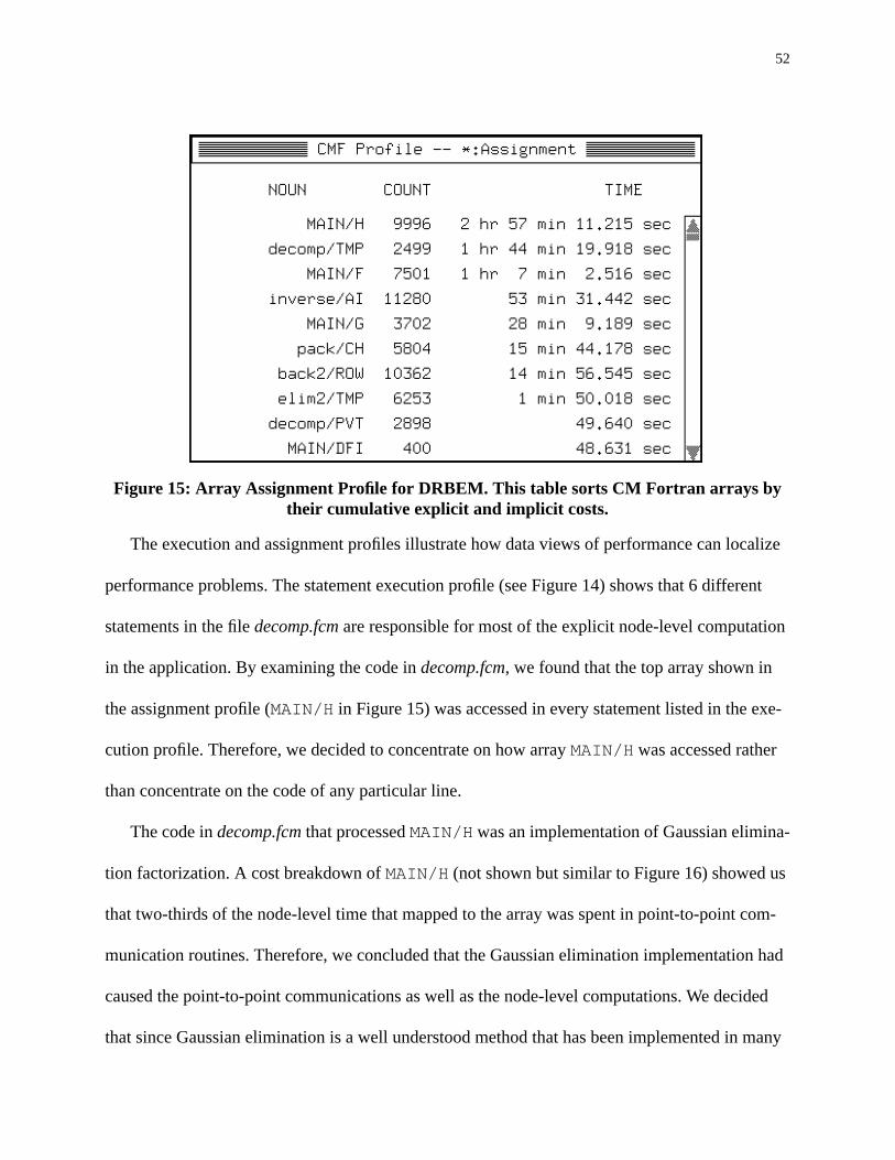
52

The execution and assignment profiles illustrate how data views of performance can localize

performance problems. The statement execution profile (see Figure 14) shows that 6 different

statements in the file decomp.fcm are responsible for most of the explicit node-level computation

in the application. By examining the code in decomp.fcm, we found that the top array shown in

the assignment profile (MAIN/H in Figure 15) was accessed in every statement listed in the exe-

cution profile. Therefore, we decided to concentrate on how array MAIN/H was accessed rather

than concentrate on the code of any particular line.

The code in decomp.fcm that processed MAIN/H was an implementation of Gaussian elimina-

tion factorization. A cost breakdown of MAIN/H (not shown but similar to Figure 16) showed us

that two-thirds of the node-level time that mapped to the array was spent in point-to-point com-

munication routines. Therefore, we concluded that the Gaussian elimination implementation had

caused the point-to-point communications as well as the node-level computations. We decided

that since Gaussian elimination is a well understood method that has been implemented in many

Figure 15: Array Assignment Profile for DRBEM. This table sorts CM Fortran arrays bytheir cumulative explicit and implicit costs.

53

linear algebra libraries, we might replace the entire subroutine with a call to a library routine.

Therefore, we replaced the routine with a call to the vendor provided CM Scientific Software

Library (CMSSL) Gaussian elimination routine. The improvement reduced the runtime of the

application by 27% as shown in the third row of Figure 13.

Figure 14 also shows large explicit computation costs for 10 lines in the file inverse.fcm.

When we examined the listed lines, we found that array MAIN/F (listed third in the assignment

profile) was accessed on 8 of the 10 lines. Again, it seemed more important to study the process-

ing of MAIN/F rather than examine any particular line. We displayed a Cost Breakdown table

(see Figure 16) and found that more than 50% of the costs of assignments involving MAIN/F

were due to point-to-point communication of elements of MAIN/F and spreading subsections of

MAIN/F across processors. We examined the use of MAIN/F on the 8 lines and identified the

operations that cause point-to-point communications and spreading of array elements. The code

lines were part of a routine that computed the inverse of matrix MAIN/F. The routine took advan-

tage of symmetries in the matrix, but we found that by employing a CMSSL routine for general

matrix inversion, we improved the execution time of the entire application by 14% as shown in

the sixth row of Figure 13.

Array assignment profiles are also useful for locating unused arrays. Unused arrays are arrays

that are specified by the programmer, allocated by the runtime system, but never used by the pro-

gram. In ParaMap they appear as CMF-level nouns, but they are not recorded in any assignment

sentences. Therefore, an array assignment profile lists unused arrays at the bottom showing no

cumulative cost. For the DRBEM application we found 16 unused arrays and improved the pro-

gram by eliminating them from the code. The runtime savings (shown in the fourth row of

Figure 13) were 2%, and the memory savings amounted to 32 Megabytes (5% of the total).

54

The final major performance problem involved sequential subroutine execution time. Subrou-

tine execution time is measured as process time on the control processor and is measured for each

subroutine in the application. We displayed a profile of subroutine execution and found that 27

minutes were spent in the subroutine solve2. The subroutine implemented the solution phase of

the application and had apparently never been parallelized. We decided that the vendor provided

CMSSL parallel linear system solver could be used to improve runtime performance, and inserted

the CMSSL solver in place of solve2. This change reduced the overall runtime of the program

by 34% as shown in the fourth row of Figure 13.

Figure 17 illustrates key aspects of the behavior of the DRBEM application over time. The

figure presents the process time spent performing point-to-point communications of elements of

arrays MAIN/H and MAIN/F, and serial time spent in subroutine solve2. The figure shows that

the implicit communications and the serial computations degraded the performance of the appli-

cation by using a significant amount of the parallel processing resources of the machine. In partic-

Figure 16: Cost Breakdown for assignment operations involving MAIN/F. The table showsthat most low-level operations involving the array were implicit and caused communication

55

ular, during the 27 minutes in which solve2 executed on the control processor, all of the

processor nodes remained idle. The final line of Figure 13 presents the total savings achieved by

incorporating all of the improvements listed above.

5.4 Summary

Even a simple tool based on the NV model can have great advantages when studying the perfor-

mance of programs written in high-level parallel languages. With ParaMap, we answered perfor-

mance questions that could not easily be answered with other tools. In particular, we used data

views of performance to quickly localize primary performance problems, and we then examined

runtime system and processor activities (while maintaining references to high-level arrays and

sub-sections of arrays) to evaluate the low-level results of array operations. Specific examples of

this type of analysis include the localization of broadcasts to a particular portion of an array in

Section 5.3.1, and attribution of point-to-point messages to a few important arrays in Section

Figure 17: Time plot of CPU Time for the entire initial parallel DRBEM application. Thedisplay shows three primary runtime contributors: Point-to-Point communications thatmap to arrays MAIN/H and MAIN/F, and sequential execution in the routine solve2

56

5.3.2. ParaMap finds problems that could be found with simple profilers (such as sequential pro-

cessing bottlenecks in subroutines), but by employing NV mapping functions, providing access to

array information, and providing time plots of performance data, ParaMap allows programmers to

go beyond traditional performance measurement analysis techniques and study more difficult

problems.

We have found that providing performance information for the fundamental constructs of a

language (e.g. parallel arrays in CM Fortran) provides a good first step in understanding any

application’s performance. However, when we have located an array with high performance costs,

we have used ParaMap to drop down to the runtime system or node level to evaluate the object’s

impact ($) on the system. We have then used the tool to determine whether the cumulative costs

are due to the programmer’s explicit requests for computation or whether the programmer has

implicitly (and perhaps unknowingly) caused extra runtime activity. This type of analysis repre-

sents a departure from high-level language tools that provide information exclusively at the lan-

guage level.

57

6. The NV Model withDynamic Instrumentation

To provide source-level views of performance, the ability to peel back layers of abstraction, and

data views of performance, a performance tool must be flexible. Although the ParaMap tool pro-

vided us with important insights into the problem of building tools for high-level parallel pro-

gramming languages, it is limited by its use of static instrumentation for gathering performance

data and mapping information. Static performance instrumentation limits performance data to a

relatively small amount that can be collected at runtime without large perturbations of execution

performance, large amounts of disk storage, and expensive performance analysis. Similarly, static

mapping instrumentation limits the relationships between levels of abstraction that can be used by

the tool. With dynamic instrumentation of dynamic mapping information, our tools may use the

exact mapping information they need, when they need it.

In this chapter, we discuss the Paradyn parallel program performance measurement tool and

describe the Paradyn features that support source-level performance data, mapping of perfor-

mance data between levels of abstraction, and data views of performance. We first describe the

design of Paradyn and its use of dynamic performance instrumentation. We then describe how we

have extended Paradyn with interfaces for both static and dynamic mapping information. The

interfaces allow Paradyn to be used with any language system that can provide mapping informa-

tion. In particular, we describe how Paradyn imports static mapping information from the CM

Fortran compiler and dynamic mapping information from the CM runtime system.

58

Finally, we describe performance measurement experiments with three real CM Fortran appli-

cations not measured in previous chapters. With each of the three experiments, we use Paradyn to

examine CMF-level views of performance, peel back layers of abstraction when needed, and

examine data views of performance. We find that data views of performance are consistently use-

ful, whether used alone or in combination with code views, in helping to explain performance

characterisitcs of data-parallel programs. We attempt to improve the performance of each applica-

tion, and in all cases we achieve significant overall execution time improvements (15-50%) across

a range of input sizes.

6.1 The Paradyn Parallel Program Performance Measurement Tool

Paradyn is a performance measurement tool that uses dynamic instrumentation to measure only

the performance data requested by users. Paradyn starts an application executing, waits for user

requests to measure performance metrics, instruments the running application (usually by rewrit-

ing the application’s executing binary image), and then sends a stream of performance measure-

ments back to the user. By limiting its instrumentation to only requested data, Paradyn can greatly

reduce instrumentation intrusion and allows users to measure large, long-running applications on

large-scale parallel computers. Paradyn includes performance display modules that allow users to

view performance metric streams graphically during the execution of their applications. Paradyn

also includes an automated module (called the Performance Consultant) to help users find perfor-

mance problems in their applications. The Performance Consultant uses a formal search strategy

to automatically find and notify the user of performance problems.

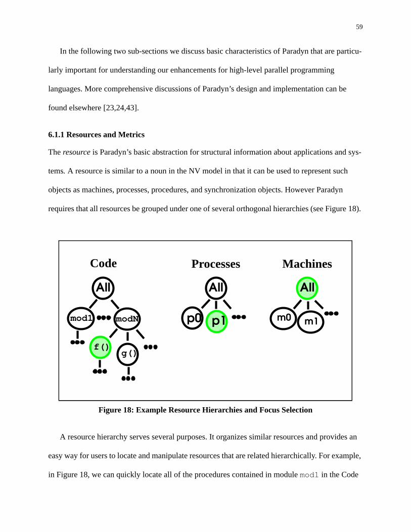
59

In the following two sub-sections we discuss basic characteristics of Paradyn that are particu-

larly important for understanding our enhancements for high-level parallel programming

languages. More comprehensive discussions of Paradyn’s design and implementation can be

found elsewhere [23,24,43].

6.1.1 Resources and Metrics

The resource is Paradyn’s basic abstraction for structural information about applications and sys-

tems. A resource is similar to a noun in the NV model in that it can be used to represent such

objects as machines, processes, procedures, and synchronization objects. However Paradyn

requires that all resources be grouped under one of several orthogonal hierarchies (see Figure 18).

A resource hierarchy serves several purposes. It organizes similar resources and provides an

easy way for users to locate and manipulate resources that are related hierarchically. For example,

in Figure 18, we can quickly locate all of the procedures contained in module mod1 in the Code

Figure 18: Example Resource Hierarchies and Focus Selection

Code Processes Machines

All

mod1 modN

f()g()

All

p0 p1

All

m0 m1

60

hierarchy. A resource hierarchy also gives Paradyn’s Performance Consultant a structure within

which it can search for performance problems. For example, if the Performance Consultant finds a

performance problem exists in source code module modN, it can refine the location of the prob-

lem by measuring the individual procedures within modN.

To collect performance data, a user must select a focus and a metric. A focus consists of

exactly one resource from each of the orthogonal resource hierarchies, and provides a canonical

representation of the requested object. For example, in Figure 18, we have one selected resource

in each of the resource hierarchies. The focus corresponding to the selection represents Procedure

f() in module modN in process p1 on all of the machines. Paradyn will automatically constrain

all performance measurements for the focus to the selected processor and the selected procedure.

The metric is Paradyn’s basic abstraction for any measurable performance quantity. Metrics in

Paradyn are similar to verbs in the NV model in that they represent application activities. The pri-

mary difference is that a verb describes an activity that can be measured with several different

metrics. For example, a verb representing procedure execution would likely correspond to Para-

dyn metrics for procedure_calls and cpu_time. The former metric counts procedure executions

while the latter metric times procedure executions. Paradyn includes a set of its own standard

metrics and allows users to add descriptions of how to collect new metrics.

To request performance data, a user chooses a list of focuses and a list of metrics and asks the

tool to collect performance data for each of the focus/metric pairs. The tool inserts the appropriate

instrumentation for the request (usually by inserting monitoring code into the running application

binary image) and sends a stream of performance data back to the user. Users include external

visualization modules, automated analysis modules such as the Performance Consultant, and

human users who interact with Paradyn’s graphical user interface.

61

6.1.2 System Structure

Paradyn is structured so that the graphical user interface, Performance Consultant, and perfor-

mance visualizations may execute on a user’s workstation while the parallel application program

executes on a remote parallel system. The block diagram shown in Figure 19 presents the basic

system structure of Paradyn. In this section, we briefly describe each of Paradyn’s primary struc-

tural elements, and in the following sections we describe our enhancements for the support of

high-level parallel programming languages.

Figure 19: Basic structure of Paradyn

application processes

daemon

datamanager

GUI PC

application processes

daemon

visualization visualization

62

Application processes (shown near the bottom of Figure 19) include any processes that the

user wishes to measure. They may execute on the same machine as the rest of Paradyn or on sep-

arate machines. Application processes are started and controlled by Paradyn daemon processes.

Paradyn daemons control application processes, handle all low-level architecture-dependent

details of dynamic instrumentation, process application symbol tables for resource information,

and transport performance data to the Paradyn front-end.

Paradyn’s fundamental representation of an application program is contained in the Data

Manager. The Data Manager exports resource hierarchies and metrics to other parts of Paradyn,

allows control of application processes, accepts requests for performance data, and sends streams

of requested performance data. The Data Manager interface is the focus of most of Paradyn’s new

capabilities for handling high-level parallel programming languages.

Several different types of modules may use the Data Manager interface. Performance visual-

ization modules (called VISIs) request performance data and graphically display the resulting

streams of performance data in such forms as time-plots, barcharts, and tables. Users may build

new external VISI programs if they wish to display data in new ways. The Performance Consult-

ant uses the Data Manager interface to request performance data when it wishes to test an hypoth-

esis about the existence or location of a performance problem. It subsequently analyzes the

returned performance stream, determines whether the hypotheses were valid, forms new hypothe-

ses, and continues its search. Finally, Paradyn’s graphical user interface allows users to communi-

cate with the Data Manager to control process execution. Users may start new processes, pause

currently running processes, or continue the execution of paused processes.

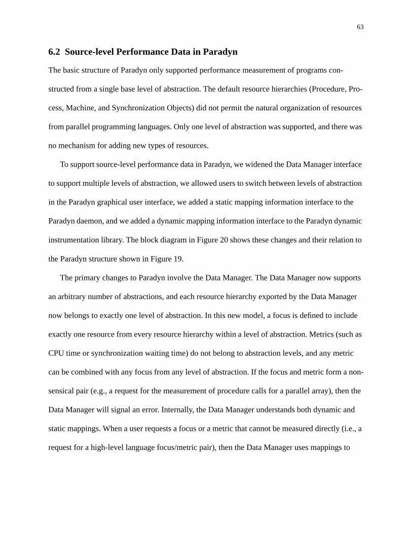
63

6.2 Source-level Performance Data in Paradyn

The basic structure of Paradyn only supported performance measurement of programs con-

structed from a single base level of abstraction. The default resource hierarchies (Procedure, Pro-

cess, Machine, and Synchronization Objects) did not permit the natural organization of resources

from parallel programming languages. Only one level of abstraction was supported, and there was

no mechanism for adding new types of resources.

To support source-level performance data in Paradyn, we widened the Data Manager interface

to support multiple levels of abstraction, we allowed users to switch between levels of abstraction

in the Paradyn graphical user interface, we added a static mapping information interface to the

Paradyn daemon, and we added a dynamic mapping information interface to the Paradyn dynamic

instrumentation library. The block diagram in Figure 20 shows these changes and their relation to

the Paradyn structure shown in Figure 19.

The primary changes to Paradyn involve the Data Manager. The Data Manager now supports

an arbitrary number of abstractions, and each resource hierarchy exported by the Data Manager

now belongs to exactly one level of abstraction. In this new model, a focus is defined to include

exactly one resource from every resource hierarchy within a level of abstraction. Metrics (such as

CPU time or synchronization waiting time) do not belong to abstraction levels, and any metric

can be combined with any focus from any level of abstraction. If the focus and metric form a non-

sensical pair (e.g., a request for the measurement of procedure calls for a parallel array), then the

Data Manager will signal an error. Internally, the Data Manager understands both dynamic and

static mappings. When a user requests a focus or a metric that cannot be measured directly (i.e., a

request for a high-level language focus/metric pair), then the Data Manager uses mappings to

64

translate the request into an equivalent request consisting of focus/metric pairs that it can measure

directly. It then passes on these mapped focus/metric pairs to the Paradyn daemons for generation

of instrumentation requests.

6.3 Mapping of Performance Data Between Levels of Abstraction

Paradyn receives information about new levels of abstraction, new resources, and new metrics

from two mapping information interfaces. Paradyn daemons import static mapping information

via Paradyn Information Format (PIF) files just after they load each application executable. PIF

Figure 20: Updated Paradyn structure.

datamanager

GUI PC

application processes

daemon

dynamic

static

abstractionsresourcesmetricsmappings

language-specificvisualizations

a = f(b)c = sum(a)d = a - cforall a b = b+1 c = sumforall d x = y*z

mappinginformation

mappinginformation

65

files are emitted by compilers, programming environments, or other external sources that wish to

define source-level language code and data objects that are contained in an application. PIF files

allow such tools to explain to Paradyn how it should map requests for high-level language

resources and metrics into requests for base resources and metrics such as functions and CPU

time. The PIF format also allows external tools to communicate descriptive information about

resources and metrics to Paradyn. In this way, language-dependent and application-dependent

visualization modules can receive descriptive information to add meaning to visual displays.

The Paradyn dynamic instrumentation library sends dynamic mapping information to the

Paradyn daemon process using the same communication channel used for performance data. The

dynamic instrumentation library, linked into every application program that is measured by Para-

dyn, contains interface procedures that allow the application to describe mappings while it exe-

cutes. The dynamic instrumentation library sends the mapping information to the Paradyn

daemons, and the daemons forward the mapping information to the Data Manager. The Data

Manager uses the dynamic mapping information in exactly the same way as it uses static mapping

information.

Paradyn uses dynamic performance instrumentation techniques to turn on or turn off the flow

of dynamic mapping information. Dynamic instrumentation allows applications to avoid the cost

of emitting mapping information when they are not run with Paradyn and allows Paradyn users to

turn off mapping information collection when it is not needed. Currently, Paradyn allows users to

turn on or turn off all dynamic mapping instrumentation points at once. Eventually, we could tie

the enabling and disabling of individual mapping instrumentation points to requests for perfor-

mance information.

66

6.4 CM Fortran-Specific Resources and Metrics

Using the static and dynamic mapping interfaces described above, Paradyn measures important

resources and metrics that are unique to CM Fortran and the CM Runtime System (CMRTS). In

this section we describe the details of how Paradyn measures performance data for CM Fortran’s

parallel assignment statements and parallel arrays and measures CMRTS-specific activities such

as Broadcast Messages, Point-to-Point Messages, Reductions, and Argument Processing.

6.4.1 Performance Data for Parallel Arrays

Arrays are the fundamental source of parallelism in data-parallel CM Fortran. They are the only

data objects that use memory on the nodes of a CM-5 system, and the performance of any partic-

ular CM Fortran program depends greatly on its efficiency of computation and communication of

arrays.

Paradyn measures CM Fortran arrays in a two step process. First, Paradyn’s dynamic instru-

mentation library detects array allocations (and deallocations) and forwards resource and map-

ping information to Paradyn. When an array is allocated (via a call to a particular CMRTS

allocation routine) the dynamic instrumentation library notifies Paradyn of the new array, estab-

lishes a unique identifier for the array, and tells Paradyn (via the dynamic mapping interface

described in Section 6.3) which subregion of the array is stored on which node of the system.

Paradyn uses this information to build a CMFarrays hierarchy as shown in Figure 21. The figure

shows that the module bow.fcm contains six functions, and one of those (CORNER) contains five

arrays. One of the arrays within CORNER (called TOT) has been expanded to show its subre-

gions.

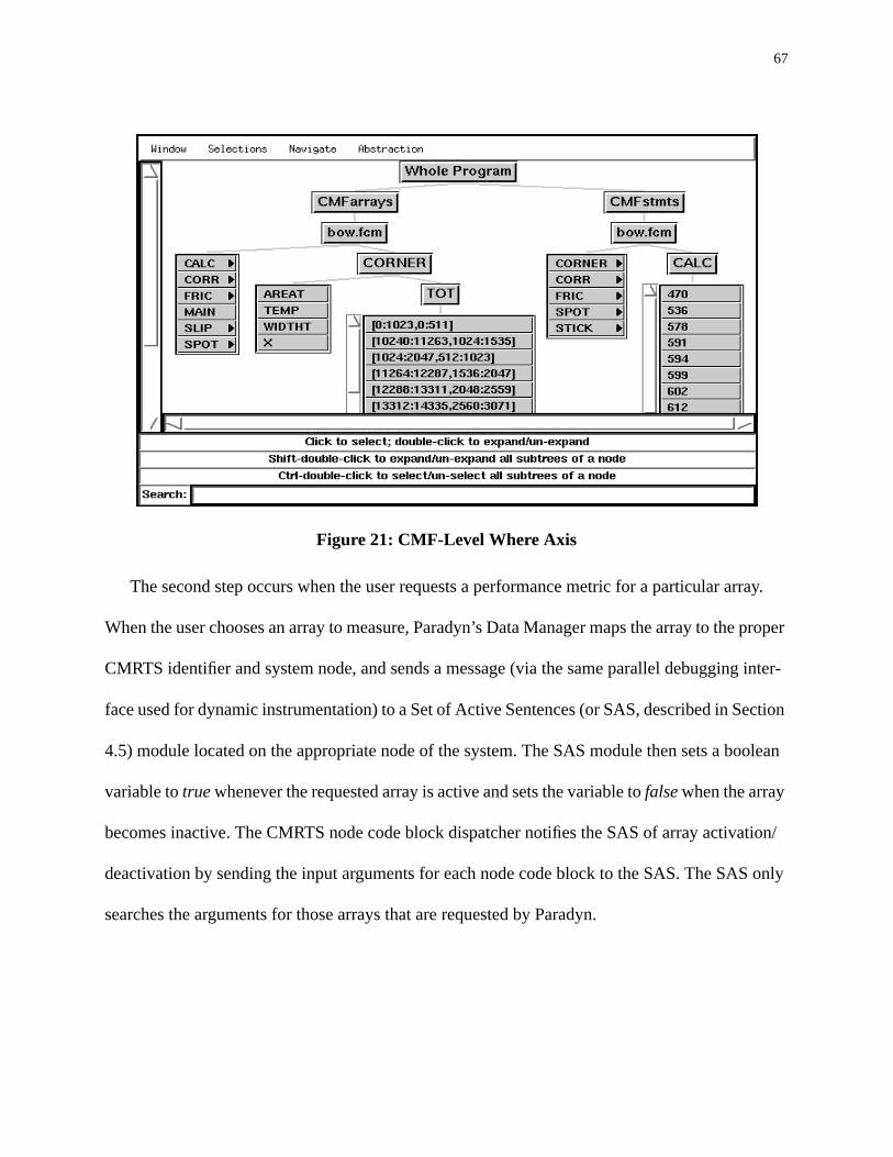
67

The second step occurs when the user requests a performance metric for a particular array.

When the user chooses an array to measure, Paradyn’s Data Manager maps the array to the proper

CMRTS identifier and system node, and sends a message (via the same parallel debugging inter-

face used for dynamic instrumentation) to a Set of Active Sentences (or SAS, described in Section

4.5) module located on the appropriate node of the system. The SAS module then sets a boolean

variable to true whenever the requested array is active and sets the variable to false when the array

becomes inactive. The CMRTS node code block dispatcher notifies the SAS of array activation/

deactivation by sending the input arguments for each node code block to the SAS. The SAS only

searches the arguments for those arrays that are requested by Paradyn.

Figure 21: CMF-Level Where Axis

68

To collect metrics, Paradyn dynamically inserts instrumentation code into node-level subrou-

tines. If a metric is to be measured for an array, then the dynamically-inserted instrumentation

code checks the array’s node-global boolean variable (discussed above), before measuring the

metric. Paradyn can thereby constrain any metric to an array of interest.

Paradyn can easily use its existing visualization modules (time plots, bar charts, and tables)

for visual display of performance information for data objects. These visualization modules sim-

ply treat a data object as a resource like any other. However, Paradyn’s visualization interface is

open; we could build specialized visualization modules to take advantage of properties (such as

geometric structure) that are unique to arrays.

6.4.2 Parallel Code Constructs

Parallel code constructs allow CM Fortran programmers to manipulate parallel arrays. Code con-

structs include parallel assignment statements, FORALL iterators, and intrinsic operations such as

SUM, MIN, and TRANSPOSE.

Paradyn measures parallel code constructs by mapping each statement to the node code blocks

that implement it. Paradyn receives this mapping information via PIF files as described in Section

6.3. We create CM Fortran PIF files with a simple utility that parses CM Fortran compiler output

files. The utility scans the compiler output files for lists of parallel statements, parallel arrays, and

node-code blocks. It then produces a PIF file that defines the statements and arrays for Paradyn

and describes the mappings from statements to code blocks.

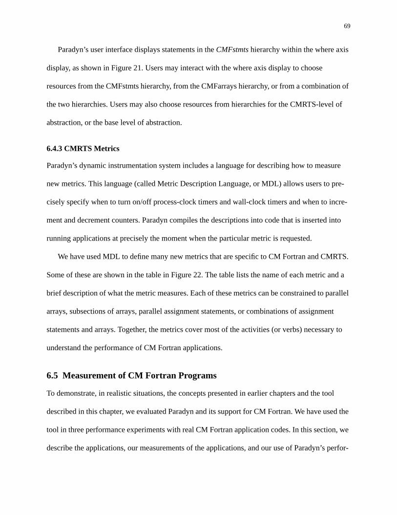
69

Paradyn’s user interface displays statements in the CMFstmts hierarchy within the where axis

display, as shown in Figure 21. Users may interact with the where axis display to choose

resources from the CMFstmts hierarchy, from the CMFarrays hierarchy, or from a combination of

the two hierarchies. Users may also choose resources from hierarchies for the CMRTS-level of

abstraction, or the base level of abstraction.

6.4.3 CMRTS Metrics

Paradyn’s dynamic instrumentation system includes a language for describing how to measure

new metrics. This language (called Metric Description Language, or MDL) allows users to pre-

cisely specify when to turn on/off process-clock timers and wall-clock timers and when to incre-

ment and decrement counters. Paradyn compiles the descriptions into code that is inserted into

running applications at precisely the moment when the particular metric is requested.

We have used MDL to define many new metrics that are specific to CM Fortran and CMRTS.

Some of these are shown in the table in Figure 22. The table lists the name of each metric and a

brief description of what the metric measures. Each of these metrics can be constrained to parallel

arrays, subsections of arrays, parallel assignment statements, or combinations of assignment

statements and arrays. Together, the metrics cover most of the activities (or verbs) necessary to

understand the performance of CM Fortran applications.

6.5 Measurement of CM Fortran Programs

To demonstrate, in realistic situations, the concepts presented in earlier chapters and the tool

described in this chapter, we evaluated Paradyn and its support for CM Fortran. We have used the

tool in three performance experiments with real CM Fortran application codes. In this section, we

describe the applications, our measurements of the applications, and our use of Paradyn’s perfor-

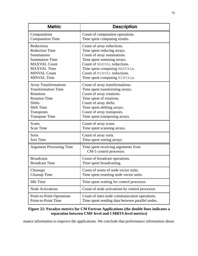
70

mance information to improve the applications. We conclude that performance information about

Metric Description

ComputationsComputation Time

Count of computation operations.Time spent computing results.

ReductionsReduction TimeSummationsSummation TimeMAXVAL CountMAXVAL TimeMINVAL CountMINVAL Time

Count of array reductions.Time spent reducing arrays.Count of array summations.Time spent summing arrays.Count of MAXVAL reductions.Time spent computing MAXVALs.Count of MINVAL reductions.Time spent computing MINVALs.

Array TransformationsTransformation TimeRotationsRotation TimeShiftsShift TimeTransposesTranspose Time

Count of array transformations.Time spent transforming arrays.Count of array rotations.Time spent of rotations.Count of array shifts.Time spent shifting arrays.Count of array transposes.Time spent transposing arrays.

ScansScan Time

Count of array scans.Time spent scanning arrays.

SortsSort Time

Count of array sorts.Time spent sorting arrays.

Argument Processing Time Time spent receiving arguments fromCM-5 control processor.

BroadcastsBroadcast Time

Count of broadcast operations.Time spent broadcasting.

CleanupsCleanup Time

Count of resets of node vector units.Time spent resetting node vector units.

Idle Time Time spent waiting for control processor.

Node Activations Count of node activations by control processor.

Point-to-Point OperationsPoint-to-Point Time

Count of inter-node communication operations.Time spent sending data between parallel nodes.

Figure 22: Paradyn metrics for CM Fortran Applications (the double lines indicates aseparation between CMF-level and CMRTS-level metrics)

71

Node-level verbs helps to explain performance problems that cannot be fully understood at the

CMF level of abstraction, that data views of performance add a useful perspective to performance

studies of CM Fortran applications, and that, in some cases, data views can localize performance

problems to a few parallel arrays, even when the problems are diffuse in code views.

6.6 Vibration Analysis (Bow)

Our first application (called Bow) simulates the oscillations of a bowed violin string [56,57]. The

application has been used to study such variables as initial transients in bowed strings, frictional

interaction at the bow-hair string interface, and stiff strings. The code consists of approximately

1200 lines of CM Fortran code contained in a single source file. By varying input parameters, we

can control the resolution of simulation, the length of simulation, and the simulation’s initial con-

ditions. The code was provided by Robert Schumacher, Professor of Physics, Carnegie Mellon

University.

We began our study of Bow by examining the overall performance characteristics of the appli-

cation as shown in Figure 23. The figure shows a time plot of three primary CMF-level metrics

and CMF Overhead for a run on a 32 node partition of a CM-5 system. The metrics are not con-

strained to any particular module, subroutine, statement, or array, but instead are collected for the

whole program. The total available time as measured by Paradyn is 16 CPUs1.

The display in Figure 23 shows that RTS-level and Node-level overhead costs dominate the

execution of Bow. Only Computation Time is significant among the CMF-level metrics and it

accounts for only a fraction of the CPU resources available to the application. The display also

1. The CM-5 allocates a full time quantum to every process that is ready to run on the CM-5’s parallelnodes, regardless of whether the process requires a full time quantum. Therefore, Paradyn’s daemon pro-cess is always allocated a full time quantum, even though it rarely requires a full time quantum to com-plete its work. Therefore, any application measured by Paradyn on a CM-5 is only allocated half of thetotal available CPU time.

72

shows that the Computation Time metric is relatively uniform over the entire execution. We con-

cluded that the majority of the application’s execution must be spent in RTS-level and Node-level

activities.

To identify the lower-level activities that consumed the majority of the CPU time available to

Bow, we peeled back layers of abstraction and examined CMRTS-level and Node-level perfor-

mance data, as shown in Figure 24. This figure shows the CMF-level Computation Time metric,

along with measurements of Idle Time (time spent waiting for the CM-5 control processor), Argu-

ment Processing Time (time spent receiving parameters for node-level code blocks), and Node

Activations (frequency of activation of the parallel nodes by the control processor).

Figure 23: CMF-level Performance Data for Bow (Scan_time and Reduction_time are eachat or near zero during entire execution)

73

We can see from the display that the cost of processing arguments and idling are higher than

the cost of computing, and that the rate of node activation is also high (over 100,000 per second or

almost once per 150 microseconds per node). These measurements suggest that each computation

activated on the nodes is a small computation.

The performance data shown in Figure 24 led us to believe that, although the application had

been partitioned properly, the application’s computational grain-size was too small for the CM-5.

We knew that the program’s authors efficiently distributed and aligned the program’s data because

there are virtually no costs associated with node-to-node messages or broadcasts (not shown).

However, the large amounts of idle time, argument processing time, and node activations indicate

Figure 24: Node-level Performance Data for Bow

74

that the control processor spends a large amount of time deciding what the parallel nodes should

do, but the nodes do not spend much time finishing their tasks. Therefore, most of the machine

waits for the control processor most of the time.

We then used a data view of performance to determine which arrays were involved in compu-

tations. We displayed Computation Time for the arrays shown in Figures 25 and 26. The time

plots in Figures 25 and 26 show the Computation Time metric constrained to four different arrays

that account for almost all of the computation activity in the application. To find these four arrays

we examined the Computation Time metric for several dozen parallel arrays and statements, and

the four shown in the figures stood out as the top users of computation resources. We also discov-

ered (not shown) that the time spent per computation on each of the arrays was very small. This

concurred with our earlier hypothesis that the computational grain-size was small.

Figure 25: Performance for Righthand Convolution Matrices.

75

When we looked at the code that manipulated these four arrays, we found several DO loops

like the one shown in Figure 27. We immediately saw why the code was not achieving full paral-

lelism. The code fragment is part of a convolution in which a small matrix is multiplied, row by

row, over a larger matrix. Each column of a given row is calculated in parallel but each row is

computed sequentially and immediately added to a running vector sum. The rows are rarely very

long, and computing each one separately does not provide enough work per computation to out-

weigh the implicit costs of starting the parallel nodes and sending them arguments for the compu-

tation. Therefore, the application does not execute efficiently on the CM-5 hardware.

Figure 26: Performance for Lefthand Convolution Matrices

ALEFT = 0.0DO I=1,LENL

ALEFT = ALEFT + (HISTL(IBACKL+I,:) * CRLEFT(I,:))END DO

Figure 27: Example of Original Convolution Code (taken from lines 635-638 of code)

76

To increase grain-size, we altered the code so that both the rows and the columns of the con-

volution matrix are executed in parallel, as shown in Figure 28. As the code fragment shows, we

allocate a temporary array (LT) to store intermediate values and we use an intrinsic parallel sum

operation to calculate the final result vector. The storage required for the new temporary vector is

relatively small because it need only be as large as the size of the convolution matrix. The results

of these changes may be seen in the time plot shown in Figure 29.

Figure 29 shows that the execution time of the application has been reduced substantially as a

result of our changes. We can now see that the Idle Time, and Argument Processing Time have

both been reduced substantially and that Computation Time has increased substantially. These

curves indicate that the parallel nodes spend more of their time doing useful work and less time

waiting for the control processor. Furthermore, the Sum Time curve in the figure shows the por-

tion of Computation Time due to Summations.

To determine whether our improvements to Bow were useful across a range of various input

parameters, we ran both versions of the application through five input sets (without Paradyn

attached). The results are shown in Figure 30. The table shows that the actual reduction in execu-

tion time for the uninstrumented application improves slightly with increased iteration size and

that the overall reduction was quite close to the change predicted by examining before (Figure 23)

and after (Figure 29) runs using Paradyn.

LT(1:LENL, :) = HISTL(B+1:B+LENL, :) * CRLEFT(1:LENL, :)ALEFT = SUM(LT, DIM=1)

Figure 28: Improved Convolution Code

77

Our measurements of the Bow application suggest that source-level views can be more useful

when augmented with lower level views of performance. We demonstrated that a perfectly paral-

lel application can have high Node-level initialization costs if it is spread thinly across parallel

nodes. In the CM Fortran execution model on the CM-5, small grain-size causes frequent node

activations, large amounts of idling while nodes wait for the control processor, large proportions

of time spent receiving code-block arguments from the control processor, and very brief computa-

tion periods on the nodes. Paradyn allowed us to describe, measure, and display the performance

of these Node-level implicit activities.

Data views of performance were especially useful (relative to code views) in focusing on the

parallel data structures used in several fine-grained computations. Although the fine-grained com-

putations were diffused among many statements, they were localized to just a few parallel arrays.

Figure 29: Paradyn Display of Improved Bow

78

There may be other performance problems and potential improvements for the Bow applica-

tion. The overall costs of implicit activities as shown by the Idle Time and Argument Processing

Time curves in Figure 29 indicate that there are still some significant costs related to implicit

activities.

6.6.1 Peaceman-Rachford PDE Solver (Peace)

Our second application, called Peace, is a partial differential equation solver that uses the Peace-

man-Rachford iteration method [50,51]. The Peaceman-Rachford method is sometimes used to

factor penta-diagonal equations. This particular implementation was written by Vincent Ervin,

Associate Professor of Mathematics at Clemson University. The code consists of approximately

1100 lines of CM Fortran code spread over five files. We can control the execution of the program

by varying the number of variables in the equation, by altering the convergence coefficient, and

varying the number of iterations..

We began our analysis of Peace by examining the costs of CMF-level verbs in a time plot, as

shown in Figure 31. The display shows that the application has two distinct phases of execution

with a substantial change in Computation Time and Array Transformation Time at the phase

IterationCount

Original Improved PercentChange

5x5 01 min 35 sec 01 min 09 sec -27%

10x10 05 min 49 sec 04 min 09 sec -29%

15x15 12 min 47 sec 09 min 02 sec -29%

20x24 26 min 51 sec 18 min 57 sec -29%

32x30 53 min 24 sec 37 min 31 sec -30%

Figure 30: Execution Times for Original and Improved Bow (all times are foruninstrumented executions of the program)

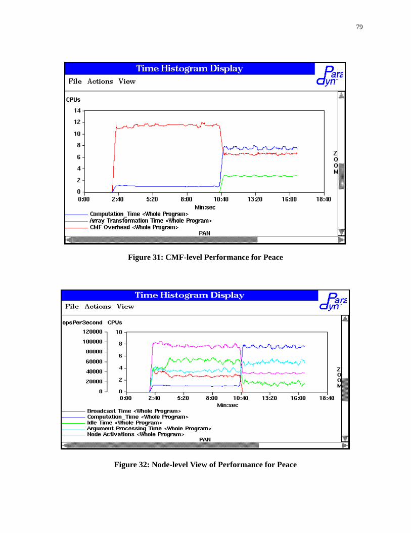
79

Figure 31: CMF-level Performance for Peace

Figure 32: Node-level View of Performance for Peace

80

boundary (approximately ten minutes, forty seconds into execution). The first phase exhibits rela-

tively low costs associated with CMF-level verbs and high overhead costs, while the second

phase shows much more parallel node utilization for CMF-level verbs.

We investigated implicit, Node-level costs in the first phase by moving to the CMRTS level of

abstraction and displaying metrics as shown in Figure 32. The display shows relatively high costs

for implicit verbs such as processing parallel code block arguments, broadcasting, and activating

parallel code blocks. Little time is spent doing actual computations during the first phase. During

the second phase, the application spends a much larger percentage of time computing with no

communication between processor nodes.

We investigated why the first phase of Bow incurred high costs for initializing the parallel

nodes of the CM-5. We used visualization displays (not shown) to find that most of the node acti-

vations in the phase were due to broadcasts, and that small amounts of data were broadcast per

activation. This information indicated that most of the costs of waiting for the control processor,

activating the nodes, and receiving code block arguments from the control processor were arti-

facts of very brief broadcasts.

We examined code views and data views to explain the cause of the broadcasts. To identify the

data being broadcast, we constrained our measurements of broadcast activity to data structures at

the CMF level. The data view in Figure 33 shows us which parallel arrays are broadcast and in

what order. Almost all of the broadcast costs are associated with three parallel arrays. The first

array (CONODE) is broadcast exclusively for over one minute and is then broadcast concurrently

with each of the other two arrays (RCONODE and BCONODE). We examined the code to find that

CONODE was computed in a special routine that used parallel assignments within sequential itera-

81

tion loops and that RCONODE and BCONODE were then computed using elements of CONODE.

The code to perform the computations of CONODE, RCONODE, and BCONODE included forty

lines of code spread over two procedures in two files.

Figure 33: Node-level Broadcasts Constrained by CMF-level Arrays

InputSize

Original Improved PercentChange

66K 3 min 14 sec 1 min 44 sec -46%

148K 6 min 39 sec 3 min 13 sec -51%

333K 14 min 35 sec 6 min 53 sec -53%

491K 22 min 1 sec 10 min 48 sec -51%

1051K 44 min 55 sec 20 min 56 sec -54%

Figure 34: Execution Times for Original and Improved Peace

82

We improved Peace by replacing all of the code that computed CONODE, RCONODE, and

BCONODE with a set of two parallel loops that compute all three arrays simultaneously. The new

code eliminates all broadcast activity and greatly reduces the execution time of the first phase of

the application. Time plots of the improved application (not shown) are similar to the second

phase of the displays shown in Figures 31 and 32.

To measure the effect of our changes, we ran the original and improved versions of Peace over

five input sets of varied size. The results, shown in Figure 34, show that the improvements help to

reduce execution time over a range of input sizes.

The second phase of Peace seems to be limited by RTS-level and Node-level implicit costs,

but as we scale up the problem set sizes, the costs of implicit activity decrease in comparison with

the costs of CMF-level explicit activity. Summary displays, such as the BarChart shown in

Figure 35, indicate that computations and array shifting now account for most of the processing

time available to the application. Furthermore, the figure indicates that two arrays (SHFTER and

AB) account for most of these costs. These two arrays are accessed in many different places in the

code (with nearly equal cost for most of the code locations), and we have not yet attempted to

improve those sections of the code.

In this experiment, source-level views of performance, lower-level metrics, and data views of

performance helped us to find and fix a significant performance problem in the Peace application.

All three techniques helped to point us to a region of execution that performed poorly, a Node-

level symptom of poor performance, and a CMF-level cause of Node-level activities. As in the

Bow application, data views of performance helped us more than code views as the performance

problem was localized to a few arrays but diffused over many statements of code.

83

6.6.2 Particle Simulation (PSICM)

Our third application (called PSICM) is a three-dimensional particle simulation code used in com-

putational fluid dynamics studies of hypersonic flow and studies of plume flowfields [11,10]. The

code consists of over 6500 lines of code in eleven source files. Input sets vary in size according to

the geometry of the flow field, the number of particles simulated, and other factors. The code was

written by a group of computational scientists at the Numerical Aerodynamic Simulation Labora-

tory of NASA Ames Research Center.

We began our study of PSICM by displaying its CMF-level performance characteristics as

shown in Figure 36. The figure shows a time plot of five CMF-level metrics over a brief run on a

32 node partition of a CM-5 system. The display shows two distinct phases of execution with a

transition from the first phase to the second phase at approximately six minutes, thirty seconds

into execution. Paradyn measured several different verbs in the the first phase, including permuta-

Figure 35: Summary of Improved Version of Peace

84

tions of array elements, parallel computations, sorts, and scans. However, the second phase of

execution is dominated by implicit costs associated with RTS-level and Node-level verbs (labeled

CMF-Overhead in the display).

To identify the lower-level activities that consumed the majority of the CPU time available to

the application in its second phase, we peeled back layers of abstraction and examined RTS-level

and Node-level verbs, as shown in Figure 37. This figure shows that the main components of the

CMF Overhead costs include Idle Time, Argument Processing Time, and Broadcast Time. We

used other displays (not shown) to determine that all of the parallel node activations during the

second phase of execution corresponded to broadcasts and that all of the costs of idling and pro-

cessing arguments were implicit initialization costs associated with the broadcasts..

Figure 36: CMF-level Performance for PSICM

85

We used a combination of code views and data views of performance to locate the cause of the

broadcasts in the second phase. The display shown in Figure 38 reveals that a single source code

statement was responsible for nearly all of the broadcasts in the phase. This line of code is shown

in Figure 39. The statement writes elements of eleven different arrays to a file. Normally, writes to

the file system would proceed relatively quickly, but because these particular arrays were allo-

cated on the parallel nodes of the system, their elements were transferred from the parallel nodes

to the control processor before the writes could proceed. The actual file write operations are much

less expensive than the cost of sending the data elements from the nodes to the control processor.

Figures 37 and 38 also show that the broadcast costs are especially high because the elements

are transferred and written one at time. The relatively high rate of broadcasts shown in Figure 38

and the high costs of processing arguments and waiting for the control processor shown in

Figure 37: Node-level Performance Data for Second Phase of PSICM

86

Figure 37 indicate that each element incurs the full cost of node activation. Furthermore, when we

divide the broadcast costs into the components responsible for each array (Figure 38 shows

broadcast frequencies for three such arrays), we see that each array is sent separately.

Figure 38: Code and Data Views of Performance for Second Phase of PSICM (note thatboth code and data views are visible in this figure)

write(fp): (cell_d(i),i=1,l),(cell_t(i),i=1,l),: (cell_r(i),i=1,l),(cell_vib(i),i=1,l),: (cell_u(i),i=1,l),(cell_v(i),i=1,l),: (cell_w(i),i=1,l),(cell_bad(i),i=1,l),: (cell_u2(i),i=1,l),(cell_v2(i),i=1,l),: (cell_w2(i),i=1,l)

Figure 39: Statement #585 in routine PRINT_STATE, in file id_part.fcm

87

We could not eliminate the need for transferring the array elements from the parallel nodes to

the control processor. Instead, we reduced the implicit costs associated with the transfer.

Figure 40 shows our new code. The new code gathers all of the separate one-dimensional arrays

into a single two-dimensional array, transfers the new array from the nodes to the control proces-

sor with a single transfer operation, and finally writes the array to file. Our new code triples the

memory space required for the cell arrays, but, if we were to make permanent changes to the

code, we could keep all of the one-dimensional arrays packed into a two-dimensional array

throughout the entire execution and avoid the use of additional space.

The time plot in Figure 41 shows the performance of the improved PSICM. The display shows

that at the transition from the first phase to the second phase, there is a single Broadcast request

followed by a relatively short period of Broadcast Time. The implicit costs associated with node

activations are nearly eliminated during this phase.

c gather parallel arraysallcell(1,:) = cell_dallcell(5,:) = cell_uallcell(6,:) = cell_vallcell(7,:) = cell_wallcell(2,:) = cell_tallcell(3,:) = cell_rallcell(4,:) = cell_viballcell(8,:) = cell_badallcell(9,:) = cell_u2allcell(10,:) = cell_v2allcell(11,:) = cell_w2

c transfer all cell arrays to FEcall cmf_fe_array_from_cm(allcell_fe, allcell(:,1:l))

c write arrays to filewrite(fp) allcell_fe

Figure 40: Improved PSICM Code

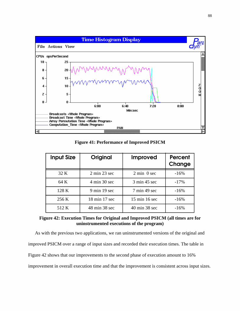
88

As with the previous two applications, we ran uninstrumented versions of the original and

improved PSICM over a range of input sizes and recorded their execution times. The table in

Figure 42 shows that our improvements to the second phase of execution amount to 16%

improvement in overall execution time and that the improvement is consistent across input sizes.

Figure 41: Performance of Improved PSICM

Input Size Original Improved PercentChange

32 K 2 min 23 sec 2 min 0 sec -16%

64 K 4 min 30 sec 3 min 45 sec -17%

128 K 9 min 19 sec 7 min 49 sec -16%

256 K 18 min 17 sec 15 min 16 sec -16%

512 K 48 min 38 sec 40 min 38 sec -16%

Figure 42: Execution Times for Original and Improved PSICM (all times are foruninstrumented executions of the program)

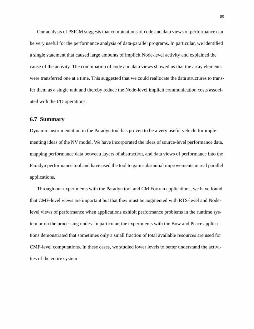
89

Our analysis of PSICM suggests that combinations of code and data views of performance can

be very useful for the performance analysis of data-parallel programs. In particular, we identified

a single statement that caused large amounts of implicit Node-level activity and explained the

cause of the activity. The combination of code and data views showed us that the array elements

were transferred one at a time. This suggested that we could reallocate the data structures to trans-

fer them as a single unit and thereby reduce the Node-level implicit communication costs associ-

ated with the I/O operations.

6.7 Summary

Dynamic instrumentation in the Paradyn tool has proven to be a very useful vehicle for imple-

menting ideas of the NV model. We have incorporated the ideas of source-level performance data,

mapping performance data between layers of abstraction, and data views of performance into the

Paradyn performance tool and have used the tool to gain substantial improvements in real parallel

applications.

Through our experiments with the Paradyn tool and CM Fortran applications, we have found

that CMF-level views are important but that they must be augmented with RTS-level and Node-

level views of performance when applications exhibit performance problems in the runtime sys-

tem or on the processing nodes. In particular, the experiments with the Bow and Peace applica-

tions demonstrated that sometimes only a small fraction of total available resources are used for

CMF-level computations. In these cases, we studied lower levels to better understand the activi-

ties of the entire system.

90

However, information about lower-level activity may not be useful unless programmers can

relate the activity to their source code. In our experiments, we have found that RTS-level and

Node-level activity can be very useful when constrained to CM Fortran code and data structures.

In each of our applications, code and data views of performance helped to identify the CMF-level

causes of RTS-level and Node-level activities.

Traditionally, performance data has been explained in terms of code constructs, but we have

shown that data views of performance can lead to more focused explanations of performance. In

two of our three experiments we found performance problems to be localized among a few paral-

lel arrays while being diffused among many code statements. We believe that data views of per-

formance will often be helpful in understanding data-parallel programs because data is the

primary source of parallelism and synchronization in such programs. In the particular cases that

we have studied, the applications allocated large data structures at the beginning of execution and

then used many routines to transform the data structures. The result is that performance problems

often can be found and fixed by concentrating on a program’s use of data structures as well as

code structures.

91

7. Conclusions

7.1 Summary

As parallel computers become larger and more complex, programmers will need good tools to

help write effective, efficient programs. With this dissertation we have addressed the unique prob-

lems that lie between two of these tools: high-level parallel languages and performance measure-

ment tools. We have explained why performance tools for parallel programming languages must

converse with programmers using the terms of the source code language, emphasized the impor-

tance of measuring implicit activity and relating it to high-level language constructs, and

described the importance of data-oriented views of performance. We have discussed each of these

problems within an informal framework (the NV Model), and described initial implementations

of their solutions in the context of the ParaMap and Paradyn performance tools. Finally, we have

demonstrated the real benefits of our ideas by using high-level language performance tools to

measure and substantially improve the performance of several real parallel applications.

Of our main ideas, the most basic is that performance tools should present performance data at

the source-code level. With high-level performance data, programmers can immediately under-

stand the overall performance characteristics of their applications and begin to grasp the perfor-

mance details of their algorithms. In the NV model, source-level data includes all performance

information that is mapped to nouns and verbs at the source code level. We have shown how we

used static techniques to map such data in ParaMap and we have shown how we used dynamic

92

mapping interfaces in Paradyn. In our measurement studies, we consistently used the high-level

views first when trying to understand the performance of application programs.

However, as we have emphasized throughout this dissertation, high-level performance infor-

mation is not always sufficient. Abstract programming systems hide details of particular hardware

and use implicit low-level activities to maintain the illusion of the programming model. In most

of our case studies, we found at least one phase of execution in which low-level implicit activity

dominated the activities of the measured application. In those cases, we peeled back layers of

abstraction to find the particular implicit activities that caused the performance problems. How-

ever, low-level performance information is of limited use unless it can be related to high-level

code structures and data structures. In our measurements, we consistently related low-level,

implicit communications to CM Fortran statements and arrays. This allowed us to locate the array

or statement that ultimately required the implicit activity.

We made all of our performance improvements at the source code level. We found that knowl-

edge of low-level performance costs, and localization of those costs to the high-level code struc-

tures and data structures that required them, allowed us to alter high-level code so that it could be

more effectively mapped to parallel hardware by the compiler. We believe that this is a good gen-

eral strategy for achieving parallel efficiency without sacrificing portability.

We have found data-oriented views of performance to be very effective. A data view of per-

formance relates performance measurements to the data-structures that are processed by a pro-

gram. In the NV model, a data structure can be measured, mapped, and profiled like any other

noun. In the ParaMap and Paradyn tools we implemented data views as simple time plots, bar

charts, and tables — the same general techniques we use for code-oriented views. Data views give

a completely new perspective of application performance and provide a dimension that is orthog-

93

onal to the traditional code views found in most performance tools. Furthermore, we have shown

that orthogonal code and data views can be combined to localize performance problems when

either view is insufficient alone. For example, we found in several data-parallel applications that

performance problems were diffuse when observed in code views (spread across many state-

ments, loops, and subroutines) but focused when observed in data views (constrained to a few

parallel vectors or matrices).

Finally, we have shown that high-level performance data, mapping between levels of abstrac-

tion, measurement of implicit activity, and data views of performance can be used to attain sub-

stantial improvements with real parallel applications. We have implemented each of these ideas in

two performance tools and have used the tools to investigate two parallel programming languages

and several parallel applications. In this dissertation, we have reported results for six of these

applications and have used the performance tools to obtain significant execution improvements in

all of them. We hope that these successes foreshadow future productivity for programmers who

use high-level parallel programming languages and performance measurement tools.

7.2 Future Work

We have encountered a large number of interesting ideas and questions during the course of com-

pleting this dissertation, and unfortunately we have been able to only address a few of them.

Therefore, we now document a few of these ideas and questions in the hope that they may be

addressed in the future.

Although we achieved success with application codes, we used an informal iterative process

augmented with educated guesses. We often needed several runs and long tedious searches for

performance problems. The computer certainly should help to automate these searches, especially

in a dynamic, on-the-fly environment such as Paradyn. Paradyn includes a dynamic Performance

94

Consultant module that is designed to discover performance anomalies, but it has yet to be

applied to high-level language applications.

There are at least two significant problems with automating the search for performance prob-

lems in high-level language programs. First, performance tools must understand, identify, and

locate performance problems that confront applications written in a particular language. We do

not know if there is a general set of such performance problem hypotheses that cover all combina-

tions of applications, languages, and systems, or if we must develop new hypotheses for each.

Second, we do not know whether searches for performance problems can take advantage of

abstraction levels. Intuitively, abstractions group related nouns and verbs and reduce the complex-

ity of the search space. It seems that searches for performance problems might be shorter if we

start at the highest level of abstraction and work downward when necessary. Alternatively, we

might attempt to find general low-level problems and then explain them in terms of the source

code language.

General, automated search for performance problems leads to the question of whether perfor-

mance is portable across hardware platforms. Tuning an application for a particular hardware

platform may lead to improvements on all hardware platforms or may lead to an application that

performs well on only one platform. In this dissertation we have successfully improved applica-

tions by making adjustments at the source code level. We presume that source-level improve-

ments are portable, but until we run the same code on several platforms, we cannot be sure. High-

level parallel languages provide the best opportunity for making such studies because they allow

programmers to write portable code.

We would also like to know whether our own ideas are applicable to other high-level parallel

programming languages. We have successfully applied the NV model to many different kinds of

95

parallel languages, but our implementations have been limited to data-parallel Fortran. As more

languages and applications become widely distributed, we would like to support them with Para-

dyn. The ideal performance tool would be independent of the source code language, runtime sys-

tem, and hardware system used by application programs.

We must recognize that some of the most successful parallel programming systems are actu-

ally programming libraries. The NV model does not make a distinction between languages and

libraries, but we need more experience with this very important class of programming system.

The most exciting situations arise when an individual application use several such libraries at

once (e.g. an unstructured grid package, such as LPARX, implemented with PVM). Ideally, Para-

dyn will separately support each library and gracefully monitor the interactions between them.

The last time someone tried to categorize parallel languages [4], their list included several

hundred languages. Today, a similar survey might yield twice as many, and the choices are bewil-

dering. As the number of parallel programming systems increases, programmers would like to

know which programming system is the best for their purposes. The parallel programming com-

munity needs to identify the desirable characteristics of parallel programming systems and needs

to determine which languages exhibit those characteristics.

Everyone agrees that execution efficiency is an important feature of any parallel programming

system, but we should not discount the importance of usability. Usability involves how easily a

given language’s programmers can accomplish their objectives. Usability is difficult to quantify,

but we must evaluate and improve usability if we expect parallel programming to move from the

domain of a few expert programmers to a much broader community. Certainly, good performance

tools improve the usability of any programming system, and we are confident that our future work

in performance tools will contribute in this area.

96

We would also like to compare and evaluate performance tools, metrics, and automated per-

formance-problem search methods. Portable parallel programming systems, with widely available

implementations and applications, provide an ideal testbed for such comparison. The best way to

compare performance tools is to develop a suite of applications to be shared by tool developers

and researchers to provide a common ground for comparison. Because portable parallel program-

ming systems are now widely available, comparison experiments could be performed by many

researchers, and could be repeated on diverse hardware platforms by independent groups to insure

accuracy.

One way to make both languages and performance tools more usable and powerful is to allow

them to cooperate more closely. Traditionally, performance tools have relied on symbolic debug-

ging information from compilers to identify the nouns and verbs contained within a program.

However, today’s performance tools yearn for much more information about nouns, verbs, compi-

lation decisions, optimizations, code layout, potential instrumentation points, mappings, and

many other pieces of information that are known only to compilers. Some compilers make some

of this information available, but no two compilers provide the same information in the same way.

The time is right to develop a general interface that allows compilers and tools to communicate.

The result would be tools and compilers with much broader applicability than is currently possi-

ble, greater leverage for groups who wish to develop tools and compilers with modest effort or

resources, and an overall reduction in the enormous effort required to produce each new perfor-

mance tool or compiler.

Finally, we would like to apply our methods for performance measurement of high-level par-

allel languages to other complex systems. Database systems, operating systems, real-time control

systems, local-area networks, and the global Internet all use multiple layers of abstraction to hide

97

execution details, ease code development, and achieve portability. Naive use of features can lead

to enormous performance problems in all of these systems. Furthermore, low-level monitoring

seldom pinpoints the high-level causes of performance problems. We believe that the NV model

could help to understand the detailed performance characteristics of complex systems and could

lead to performance tools that redefine the state of the art.

98

8. Bibliography

[1] Vikram S. Adve, Jhu-Chun Wang, John Mellor-Crummey, Daniel A. Reed, Mark Anderson,and Ken Kennedy. An integrated compilation and performance analysis environment fordata parallel programming. Technical Report 94513-S, CRPC, 1994.

[2] Ziya Aral and Ilya Gertner. Non-intrusive and interactive profiling in Parasight. In ACM/SIGPLAN PPEALS, pages 21–30, 1988.

[3] Arvind, Steve Heller, and Rishiyur S. Nikhil. Programming generality and parallel comput-ers. Technical Report 287, MIT-LCS Computation Structures Group, 1990.

[4] H. E. Bal, J. G. Steiner, and A. S. Tanenbaum. Programming Languages for DistributedComputing Systems. ACM Computing Surveys, 21(3), 1989.

[5] Peter Bates and Jack Wileden. An approach to high-level debugging of distributed systems.In ACM SIGSOFT/SIGPLAN Software Engineering Symposium on High Level Debugging,pages 107–111, March 1983.

[6] Francois Bodin, P. Beckman, Dennis Gannon, J. Gotwals, S. Narayana, S. Srinivas, andB. Winnicka. Sage++: An object oriented toolkit and class library for building fortran andC++ restructuring tools. In OONSKI 1994, 1994.

[7] Gary Brooks, Gilbert J. Hansen, and Steve Simmons. A new approach to debugging opti-mized code. In ACM SIGPLAN Proc. on Programming Language Design and Implementa-tion, pages 1–11, 1992.

[8] D. S. Coutant, S. Meloy, and M. Ruscetta. DOC: A practical approach to source-level debug-ging of globally optimized code. In ACM SIGPLAN Proc. on Programming Language De-sign and Implementation, pages 125–134, 1988.

[9] Cray Research Inc., Chippewa Falls, WI. UNICOS File Formats and Special Files ReferenceManual, 1991.

[10] Leonardo Dagum. Three-dimensional direct particle simulation on the connection machine.Technical Report RNR-91-022, NASA Ames Research Center, 1991.

[11] Leonardo Dagum and S.H. Konrad Zhuh. Three-dimensional particle simulation of high al-titude rocket plumes. Technical Report RNR-92-026, NASA Ames Research Center, 1992.

[12] William DePauw, Richard Helm, Doug Kimelman, and John Vlissades. Visualizing the be-havior of object-oriented systems. In Object-Oriented Programming Systems, Languages,and Applications Conference, pages 326–337, May 1993.

99

[13] Ian Foster, Robert Olson, and Steven Tuecke. Productive parallel programming: The PCNapproach. In Scientific Programming Vol. 1, pages 51–66. John Wiley and Sons, Inc, No-vember 1992.

[14] Joan M. Francioni and Jay Alan Jackson. Breaking the silence: Auralization of parallel pro-gram behavior. Journal of Parallel and Distributed Computing, March 1993.

[15] A. J. Goldberg and John Hennessey. Performance debugging shared memory multiprocessorprograms with mtool. In Supercomputing 1991, pages 481–490, November 1991.

[16] S. L. Graham, P. B. Kessler, and M. K. McKusick. Gprof: A call graph execution profiler. InACM SIGPLAN Symposium on Compiler Construction, June 1982.

[17] Anoop Gupta, Margaret Martonosi, and Tom Anderson. Memspy: Analyzing memory sys-tem bottlenecks in programs. Performance Evaluation Review, 20(1):1–12, June 1992.

[18] V. Haarslev and R. Moller. A framework for visualizing object-oriented systems. In Object-Oriented Programming Systems, Languages, and Applications Conference, pages 237–244,May 1990.

[19] Michael T. Heath and Jennifer A. Etheridge. Visualizing the performance of parallel pro-grams. IEEE Software, 8(5):29–39, September 1991.

[20] J. L. Hennessy. Symbolic debugging of optimized code. ACM Transactions on Program-ming Languages and Systems, 4(3):323–344, July 1982.

[21] High Performance Fortran Forum. High Performance Fortran Language Specification - Ver-sion 1.0, January 1993.

[22] Jeffrey K. Hollingsworth, R. Bruce Irvin, and Barton P. Miller. The integration of applica-tion and system based metrics in a parallel program performance tool. In ACM SIGPLANSymposium on Principles and Practice of Parallel Programming, pages 189–200, April1991.

[23] Jeffrey K. Hollingsworth and Barton P. Miller. Dynamic control of performance monitoringon large scale parallel systems. In 7th ACM International Conference on Supercomputing,pages 185–194, July 1993.

[24] Jeffrey K. Hollingsworth, Barton P. Miller, and Jon Cargille. Dynamic program instrumen-tation for scalable performance tools. In Scalable High Performance Computing Conference,May 1994.

[25] G Hurteau, A. Singh, M. Hancu, and V. Van Dongen. Eppp performance debugger. Techni-cal Report CRIM-EPPP-94/04-11, Centre de Recherce Informatique de Montreal, May 1994.

[26] R. Bruce Irvin and Barton P. Miller. A performance tool for high-level parallel programminglanguages. In Karsten M. Decker and Rene M. Rehmann, editors, Programming Environ-ments for Massively Parallel Distributed Systems, pages 299–314. Birkhauser Verlag, 1994.

[27] Laxmikant V. Kale and Amitabh B. Sinha. Projections: A preliminary performance tool forCHARM. In International Symposium on Parallel Processing, April 1993.

[28] Carl Kesselman. Integrating performance analysis with performance measurement in paral-lel programs. Technical Report 91-03, UCLA Computer Sciences Department, 1991.

100

[29] Carol Kilpatrick and Karsten Schwan. ChaosMON: Application-specific monitoring and dis-play of performance information for parallel and distributed systems. In ACM/ONR Work-shop on Parallel Program Debugging, pages 48–59, 1991.

[30] Doug Kimelman, Pradeep Mittal, Edith Schonberg, Peter F. Sweeney, Ko-Yang Wang, andDror Zernik. Visualizing the execution of high performance fortran (HPF) programs. Tech-nical report, IBM Thomas J. Watson Research Center, October 1994.

[31] M. F. Kleyn and P. C. Gingrich. Graphtrace - understanding object-oriented systems usingconcurrently animated views. In Object-Oriented Programming Systems, Languages, andApplications Conference, pages 191–205, May 1988.

[32] Scott R. Kohn and Scott B. Baden. A robust parallel programming model for dynamic non-uniform scientific computations. In Scalable High Performance Computing Conference,May 1994.

[33] Monica S. Lam and Martin C. Rinard. Coarse-grain parallel programming in Jade. In ACMSIGPLAN Symposium on Principles and Practice of Parallel Programming, pages 94–105,April 1991.

[34] James R. Larus and Thomas Ball. Rewriting executable files to measure program behavior.Software, Practice and Experience, 24(2):197–218, February 1994.

[35] Alvin R. Lebeck and David A. Wood. Cache profiling and the spec benchmarks: A casestudy. IEEE Computer, 27(10):15–26, October 1994.

[36] Thomas J. LeBlanc, John M. Mellor-Crummey, and Robert J. Fowler. Analyzing parallelprogram executions using multiple views. Journal of Parallel and Distributed Computing,9(6):203–217, 1990.

[37] Ted Lehr, David Black, Zary Segall, and Dalibor Vrsalovic. Mkm: The mach kernel monitor:Description, examples, and measurements. Technical Report 89-131, Carnegie Mellon Uni-versity School of Computer Science, April 1989.

[38] Laura Bagnall Linden. Parallel program visualization using ParVis. In Performance Instru-mentation and Visualization, pages 157–187, New York, 1990. ACM Press.

[39] Ewing Lusk and Ralph Butler. User’s guide to the P4 parallel programming system. Techni-cal Report ANL-92/17, Argonne National Laboratory, October 1992.

[40] A. D. Malony. Program tracing in cedar. Technical Report 660, University of Illinois, Centerfor Supercomputing Research and Development, April 1987.

[41] MasPar Computer Corporation, 749 North Mary Avenue, Sunnyvale, CA. MPPE ReferenceManual, 1991.

[42] James McGraw, Stephen Skedzielewski, Stephen Allan, Rod Oldehoeft, John Glauert, ChrisKirkham, Bill Noyce, and Robert Thomas. SISAL: Streams and Iteration in a Single Assign-ment Language, Languge Reference Manual – Version 1.2. Lawrence Livermore NationalLaboratory, University of California, Davis CA, March 1985.

[43] Barton P. Miller, Mark D. Callaghan, Jonathan M. Cargille, Jeffrey K. Hollingsworth,R. Bruce Irvin, Karen L. Karavanic, Krishna Kunchithapadam, and Tia Newhall. The Para-dyn parallel performance measurement tools. IEEE Computer, 28(11), November 1995.

101

[44] Barton P. Miller, Morgan Clark, Jeff Hollingsworth, Steven Kierstead, Sek-See Lim, andTimothy Torzewski. IPS-2: The second generation of a parallel program measurement sys-tem. IEEE Transactions on Parallel and Distributed Systems, 1(2):206–217, April 1990.

[45] Barton P. Miller, Cathryn MacRander, and Stuart Sechrest. A distributed programs monitorfor Berkeley UNIX. Software-Practice and Experience, 16(2):183–200, February 1986.

[46] Barton P. Miller and Cui-Qing Yang. IPS: An interactive and automatic performance mea-surement tool for parallel and distributed programs. In 7th International Conference on Dis-tributed Computing Systems, September 1987.

[47] MIPS Computer Systems, Sunnyvale, CA. UMIPS-V Reference Manual, 1990.

[48] Bernd Mohr, Darryl Brown, and Allen Malony. Tau: A portable parallel program analysisenvironment for pC++. In International Conference on Parallel Systems, pages 29–40.Springer Verlag, September 1994.

[49] D. Nardini and C. A. Brebbia. A new approach for free vibration analysis using boundary el-ements. Boundary Element Methods in Engineering, 1982.

[50] D. W. Peaceman and H. H. Rachford. The numerical solution of parabolic and elliptic dif-ferential equations. Journal of the Society of of Industrial Applied Mathematics, 3(1):28–33,1955.

[51] Donald W. Peaceman. Fundamentals of Numerical Reservoir Simulation. Elsevier ScientificPublishing Company, 1977.

[52] Sharon Perl. Performance assertions. In 14th ACM Symposium on Operating System Princi-ples, pages 134–145, December 1993.

[53] Pure Software Incorporated, Menlo Park, CA. Quantify User’s Guide, 1993.

[54] Daniel A. Reed, Robert D. Olson, Ruth A. Aydt, Tara M. Madhyastha, Thomas Birkett,David W. Jensen, Bobby A. Nazief, and Brian K. Totty. Scalable performance analysis: ThePablo performance analysis environment. In A. Skjellum, editor, Scalable Parallel LibrariesConference. IEEE Computer Society, 1993.

[55] Patrick M. Sansom and Simon L. Peyton Jones. Profiling lazy functional languages. Techni-cal report, University of Glasgow, May 1992.

[56] Robert T. Schumacher. Self-sustaining oscillations of the bowed string. Acustica, 43:109,1979.

[57] Robert T. Schumacher. Analysis of aperiodicities in nearly periodic waveforms. Journal ofAcoustic Society of America, 91:438, 1992.

[58] Karsten Schwan, Rajiv Ramnath, Sridhar Vasudevan, and David M Ogle. A language andsystem for parallel programming. IEEE Transactions on Software Engineering, 14(4):455–471, April 1988.

[59] Zary Segall and Larry Rudolph. PIE: A programming and instrumentation environment forparallel processing. IEEE Software, 2(6):22–37, November 1985.

102

[60] Steve Sistare, Don Allen, Rich Bowker, Karen Jourdenais, Josh Simons, and Rich Title. Datavisualization and performance analysis in the Prism programming environment. In Program-ming Environments for Parallel Computing, pages 37–52. North-Holland, 1992.

[61] Richard Snodgrass. A relational approach to monitoring complex systems. ACM Transac-tions on Computer Systems, 6(2):157–196, May 1988.

[62] V. S. Sunderam. PVM: A framework for parallel distributed computing. Concurrency: Prac-tice and Experience, 2(4):315–339, December 1990.

[63] A. Sussman, J. Saltz, R. Das, S. Gupta, D. Mavriplis, and R. Ponnusamy. PARTI primitivesfor unstructured and block structured problems. Computing Systems in Engineering, 1992.

[64] S. S. Thakkar. Performance of parallel applications on a shared-memory multiprocessor sys-tem. In M. Simmons and R. Koskela, editors, Performance Instrumentation and Visualiza-tion, pages 233–256. ACM Press, 1990.

[65] Thinking Machines Corporation, Cambridge MA. CM Fortran Reference Manual, January1991.

[66] Sivan Toledo. PerfSim: An automatic performance analysis tool for data-parallel fortran pro-grams. In International Symposium on the Frontiers of Parallel Systems, February 1995.

[67] E. H. Welbon, C. C. Chen-Nui, D. J. Shippy, and D. A. Hicks. The POWER2 performancemonitor. The IBM Journal of Research.

[68] Winifred Williams, Timothy Hoel, and Douglas Pase. The MPP Apprentice performancetool: Delivering the performance of the cray T3D. In Karsten M. Decker and Rene M. Reh-mann, editors, Programming Environments for Massively Parallel Distributed Systems.Birkhauser Verlag, 1994.

[69] Winifred Williams and James Kohn. ATExpert. The Journal of Parallel and DistributedComputing, 18:205–222, June 1993.

[70] Jerry C. Yan. Performance tuning with AIMS – an automated instrumentation and monitor-ing system for multicomputers. In 27th Hawaii International Conference on System Scienc-es, pages 625–633, January 1994.

[71] Polle T. Zellweger. An interactive high-level debugger for control-flow optimized programs.ACM SIGPLAN Notices, 18(8):159–172, March 1983.