performance evaluation of train moving-block control
TRANSCRIPT

HAL Id: hal-01345437https://hal.inria.fr/hal-01345437
Submitted on 22 Sep 2016
HAL is a multi-disciplinary open accessarchive for the deposit and dissemination of sci-entific research documents, whether they are pub-lished or not. The documents may come fromteaching and research institutions in France orabroad, or from public or private research centers.
L’archive ouverte pluridisciplinaire HAL, estdestinée au dépôt et à la diffusion de documentsscientifiques de niveau recherche, publiés ou non,émanant des établissements d’enseignement et derecherche français ou étrangers, des laboratoirespublics ou privés.
Performance Evaluation of Train Moving-Block ControlGiovanni Neglia, Sara Alouf, Abdulhalim Dandoush, Sebastien Simoens,
Pierre Dersin, Alina Tuholukova, Jérôme Billion, Pascal Derouet
To cite this version:Giovanni Neglia, Sara Alouf, Abdulhalim Dandoush, Sebastien Simoens, Pierre Dersin, et al.. Per-formance Evaluation of Train Moving-Block Control. 13th International Conference on QuantitativeEvaluation of SysTems (QEST) , Aug 2016, Quebec City, Quebec, Canada. pp.348-363, �10.1007/978-3-319-43425-4_23�. �hal-01345437�

Performance Evaluation of Train Moving-Block Control�
Giovanni Neglia1y, Sara Alouf1, Abdulhalim Dandoush2, Sebastien Simoens3,
Pierre Dersin3, Alina Tuholukova1, Jérôme Billion3, Pascal Derouet3
1 Université Côte d'Azur, Inria, France
[email protected] ESME Sudria, France
[email protected] Alstom Transport, France
Abstract
In moving block systems for railway transportation a central controller periodically communicates tothe train how far it can safely advance. On-board automatic protection mechanisms stop the train if nomessage is received during a given time window.
In this paper we consider as reference a typical implementation of moving-block control for metro andquantify the rate of spurious Emergency Brakes (EBs), i.e. of train stops due to communication lossesand not to an actual risk of collision. Such unexpected EBs can happen at any point on the track andare a major service disturbance.
Our general formula for the EB rate requires a probabilistic characterization of losses and delays.Calculations are surprisingly simple in the case of homogeneous and independent packet losses. Ourapproach is computationally e�cient even when emergency brakes are very rare (as they should be) andcan no longer be estimated via discrete-event simulations.
Keywords: Emergency brakes � Communication Based Train Control (CBTC) � European Train ControlSystem (ETCS)
1 Introduction
In order to avoid collisions between consecutive trains traveling on the same track, the track is traditionallydivided in �xed sections�called blocks�and only one train at a time is allowed to be in a given block.
The increasing demand for e�cient mass transit transport requires to utilize railway infrastructure moree�ciently. The improvements of train-sidetrack wireless communications, on board processing and actuatorshave made possible the introduction in the last 15 years of moving block systems, where blocks are dynamicallycalculated. Figure 1 schematically illustrates the two di�erent approaches. The moving-block control canreduce the headway taking into account the actual distance between the trains as well as their speeds. It isbeing deployed as Communication-Based Train Control (CBTC) for urban mass transit system and is underconsideration for next generation of European Train Control System (ETCS). This is referred as ETCS level3 and is currently under standardization.
Moving-block systems require a continuous information exchange (detailed in Sec. 2) between an on boardlocal controller, called the Carborne Controller (CC) and an external ground controller, called the ZoneController (ZC) because it monitors all the trains in a given zone. Safety-critical messages are exchangedusing standard or proprietary radio technologies. If no message is received during a given interval then the
�This is an author version of the 16-page paper that has appeared in the Proceedings of QEST 2016, Quebec City, QC,Canada, August 23-25, 2016.
yCorresponding author.
1

end of block 1
maximum distanceto travel
block 1 block 2
train B train A
FIXED BLOCKS
end of train B’s block
maximum distanceto travel
train B train A
MOVING BLOCKS
train C
end of train C’s block
maximum distanceto travel
Figure 1: Fixed-block and moving-block operation.
CC will no longer have valid guarantees that train movement is still safe and will trigger an EmergencyBrake (EB). It is clearly desirable to limit the frequency of spurious emergency brakes, i.e. emergency brakesthat are simply due to losses on the wireless channel and not to a potential collision risk. Indeed spuriousemergency brakes can be themselves a cause of danger, with trains potentially blocked in tunnels, risks ofpassengers disembarking on the tracks, etc. Moreover, a spurious EB can generate legitimate EBs on thefollowing trains on the track, causing in this way major service disturbance. For this reason, the so-calledperformance based contracts can bind rail transport companies to specify the maximum number of spuriousemergency brakes over a given period of time.
In spite of their criticality, the estimation of the rate of spurious EBs is mostly based on historicaloperational data. This approach strongly limits the possibility to evaluate ahead of time the performancewhen signi�cant changes are deployed and in particular when new lines based on new technologies are built.It is often required to experimentally adapt di�erent system parameters (e.g. transmission power levels, timervalues, . . . ) after the deployment of the line, and sometimes even to deploy additional trackside equipment(e.g. radio transmitters). These di�culties are often considered one of the reasons for the delay in thestandardization of ETCS level 3. For example [8] shows that the o�cial quality of service speci�cations forthe di�erent subcomponents of the ETCS level 3 system can lead to a ridiculously high rate of spurious EBs(one every 30 minutes).
A model-based analysis can then play a fundamental role for a preliminary evaluation of the real perfor-mance of moving block control. Some work has been done in this direction following [8], and then consideringits abstraction from ETCS level 3 speci�cations mostly using Stochastic Petri Nets (SPNs) [9, 5, 1, 3, 2]. Inparticular the approach proposed in [8] to numerically solve the SPN works only under the so-called enablingrestriction, i.e. only one transition can be generally distributed and all the others should be exponential ran-dom variables. In the more realistic cases, the authors rely then on Monte Carlo simulations of the SPN. Thenaive simulation approach presented in [8] cannot manage to quantify EB rate smaller than 2 EBs per hour.Importance splitting techniques used in [9] allow to estimate much smaller rates (about 10�10 per hour). It isnot clear if the computational cost of this numerical approach is insensitive to the packet loss probability p.References [5] and [7] show how UML descriptions can be used to describe the moving block control in ETCSlevel 3 and can be automatically translated to MoDeST formal language (a process algebra-based formalism)and to SPNs, but they do not solve the problem of quantitative evaluation of such rates when losses are rare.In the very recent paper [2] Carnevali et al. use the tool ORIS to solve numerically the SPN proposed in [8, 9],without the need to rely on Monte Carlo simulations. The tool indeed overcomes the limit of the enablingrestriction thanks to recent advancements based on the method of stochastic state classes [6]. Moreover, itallows for a transient analysis of the system. As a case study, the authors consider a toy-example similar tothat in [8] leading to very high EB rates. From a preliminary analysis using their tool, it is not clear if morerealistic scenarios can be solved in a reasonable amount of time.
Our approach di�ers from the related literature in three main aspects. First, rather than moving from
2

the current proposals for ETCS level 3, we consider as reference an actual implementation of the moving-block system for metro by Alstom, one of the world largest company in the domain of rail transport andsignaling. Looking at an actual implementation has led us to identify the importance of the time-slottedoperation of the two controllers (the CC and the ZC). Indeed, the most important delay component in themessages' exchange between the CC and the ZC is due to the waiting time for the next clock tick at whichthe controller can process the message. This waiting time can be equal to hundreds of milliseconds versusthe tens of milliseconds due to network delays. This aspect was ignored in the previous literature and weshow that has to be addressed to correctly evaluate the system performance. In particular, a consequence ofthe time-slotted operation is that the EB rate exhibits non-trivial discontinuity as the timer value changes.A second (methodological) di�erence in comparison to the direction of [8] and follow-ups is that we pushas further as possible the probabilistic analysis to derive closed-formula expressions. We derive a generalformula for the rate of spurious EBs under general loss and delay processes, and a simple formula for thecase of independent and homogeneous packet losses. The analysis allows to better understand the role ofthe di�erent system parameters. On the contrary, the existing literature only relies on simulations or (in thecase of [2]) on the numerical solution of a SPN. In both cases the dependence on the system parameters ishidden. Finally, from the algorithmic point of view, it is not clear if the numerical approaches proposed untilnow can be practically used to estimate EB rates as low as in this paper. Our guess is that this is probablynot the case but, perhaps, for [9] and [2].Indeed our approach does not need to simulate rare sequences ofpacket losses and is then practically implementable.
The paper is organized as follows. In Sec. 2 we describe our assumptions about the train scenario and thedetails of the moving-block control including typical values for system parameters. Then in Sec. 3 we describeour general approach to study the system, we show that a worst case analysis is of limited utility (Sec. 3.1.2)and then move to derive a general formula for the EB rate (Sec. 3.1.3) that requires to characterize systemdelays (Sec. 3.2) and losses. The case of independent and homogeneous packet losses is considered in Sec. 3.3.Some numerical experiments are in Sec. 4. Section 5 concludes the paper and discusses how to extend ourapproach to more general loss scenarios. The most frequently used acronyms are listed in Table 1. Due tospace constraints some of the results are in the companion technical report [4].
Table 1: List of AcronymsCBTC Communication Based Train ControlCC Carborne ControllerDCS Data Communication Sub-SystemEB Emergency BrakeEOA End-Of-AuthorityETCS European Train Control SystemLOC Location reportTM validity duration Timer of a LOCZC Zone Controller
2 Scenario
Here we describe the speci�c railway scenario we consider. In our description we will refer to transmissiontechnologies and parameters typical of a urban rail network (and then of a CBTC system), but our followinganalysis does not depend on these speci�c implementation details. What is instead required is that therandom variables (r.v.s) de�ned below (train speed, distances between access points, etc.) have boundedsupport and are lower bounded by a positive constant. For a given r.v. �, we denote by �min > 0 its lowerbound and by �max <1 its upper bound.1
We consider a train moving on an in�nitely long track. The train has two WiFi On Board Modems(OBMs) with directional antennas: one is located at the front of the train, the other at the back. We refer
1 Throughout the paper Greek letters always denote random variables, while capital letters usually denote system parameters.
3

1 2 3 4 5 6 7
TZC
ControllerZone
o�set
LOCgenerate read
LOCsendEOA
lostmessage
(with probability pD)timers 1, 2 and 3are deactivated
ControllerCarborne
timer LOC1
TCC EOA processing starts
Figure 2: Illustration of LOC-EOA exchanges.
to them respectively as the blue and the red OBMs. Along the track there are pairs of closely-located WiFiAccess Points (APs), using the same channel. The pair is called a Trackside Radio Equipment (TRE). EachAP in a TRE is devoted to communicate with one of the two OBMs and is connected to an independentwired network through which the Zone Controller (ZC) can be reached. We also label the APs, the wirelesschannels and the wired networks blue or red as the corresponding OBM. Hence communications between thetrain and the ZC are possible through separate paths, each with a single wireless link.
2.1 Train Moving-Block Control
In this section we describe the detailed operation of a moving block system considering as reference thespeci�c CBTC implementation by Alstom.2
Figure 2 shows a messages exchange between the on board controller (the CC) and the ground controller(the ZC). Observe that both the controllers operate in discrete time on the basis of clock periods of hundredsof milliseconds. This is due to the fact that they are actually e-out-of-f voting systems where di�erentprocessors perform in parallel the same calculations and a time-slotted operation simpli�es the synchronismof the processors. The clock periods at the ZC and at the CC (respectively TZC and TCC) are in generaldi�erent because the subsystems are provided by di�erent vendors and also because they have di�erentcomputational loads during one period.
The most important CBTC messages are location reports (LOC) and end-of-authority ones (EOA). ALOC is a message periodically transmitted from the on board CC through the Data Communication Sub-System (DCS) to the ground ZC. The message is actually sent twice through the blue and the red networks.The �rst LOC arriving at the ZC is processed. Each LOC is acknowledged by an EOA message in the reversedirection (again sent through the two networks). The EOA communicates to the CC how far the train canadvance. The LOC has a validity duration TM and a timer with such duration is activated at the generationof the LOC. An EOA is said to be valid if the timer of the corresponding LOC has not expired yet. TheCC-ZC-CC exchange works as follows.
1. A LOC is generated at the CC every TLOC , multiple of the CC clock period TCC .
2. The LOC (say LOC k) is ready to be emitted and passed to the DCS after a processing delay equal toTCC .
3. The delivery delay introduced by the DCS is a random variable �1 with support in [TDCS;min; TDCS;max].
4. At the ZC the LOC is available for computing at the next tick of the clock.
5. The computing time at the ZC required to process the LOCs from all the trains in the zone and generatethe corresponding EOAs is TZC .
2 The parameters' values have been slightly changed and some speci�c implementation details are hidden to protect Alstomindustrial know-how.
4
6. The EOA k is emitted within the next cycle of the ZC at an o�set O depending on the train.
7. The EOA is delivered to the CC after a random delay �2, distributed as �1, but independent from it.
8. At the CC the EOA gets in a processing queue, at the next tick of the CC clock the most recent EOApresent in the queue is processed unless there are higher priority tasks arrived during the same CCclock period (which happens with probability pD). In any case an EOA processing is not delayed morethan an additional CC period.
9. The EOA k is actually processed only if it remains valid until the end of the current CC clock. Onceprocessing starts, all the pending timers for older LOCs (i.e. LOC h for h � k) are deactivated.
10. If the timer of a LOC is not deactivated before its expiration, the EB procedure is triggered.
In what follows we refer to the k-th LOC and its corresponding EOA as the k-th LOC-EOA exchange,but note that any later EOA can disactivate the timer of the k-th LOC. We say that a LOC-EOA exchangeis lost if either the LOC or the EOA does not arrive to destination.
Table 2: Notation and typical values for the variables. In the paper some of the variables appear withsubscripts. A subscript b (r) denotes that the variable refers to the blue (red) OBM or network. A subscriptL (E) denotes that it refers to a LOC (an EOA).
Symbol Quantity Value
TZC ZC clock period 378 msTCC CC clock period 225 msTLOC LOC generation period 3TCCTM validity duration of a LOC 5:5 sTDCS transmission delay [10; 50] ms� positive random component of TDCS [0; 40] ms� positive random component of TDCS for �rst message to arrive [0; 40] msO EOA transmission o�set [0; TZC ]!CC number of CC ticks an EOA waits until CC processes it f0; 1gpD probability that !CC is 1 0:01!ZC time interval between LOC arrival at ZC and next ZC tick� time interval between earliest arrival time of a LOC at ZC and next ZC tickqEB emergency brake probabilityrEB emergency brake ratep packet loss~p probability to lose a LOC-EOA exchangeTk arrival time of k-th EOA k tick at which k-th EOA is processedDk event that k-th EOA is late to deactivate the timer of LOC 1Tk event that k-th LOC experiences a timeoutLk event of k-th LOC-EOA exchange loss
3 Analysis
In this paper we consider that the system is described by a stationary stochastic process and calculatethe steady-state rate at which emergency brakes occur (as common to all the related literature but [2]). Inparticular we consider that the train is moving according to some stationary mobility model and the algorithmdescribed above is running all the time, even after the occurrence of an emergency brake. Ignoring the trainstopping time after an EB is a reasonable approximation because we are estimating rare events.
5

Figure 3: Di�erent delay components of the k-th LOC-EOA exchange for two di�erent values of the LOCtransmission delay �0L;k and �
00
L;k.
We denote by Lk the event that the exchange k is lost, Tk the event that the k-th LOC experiences atimeout and �A the complement of set A. The k-th LOC experiences a timeout if the k-th exchange is lost andthe later EOAs do not arrive or arrive too late, then Tk � Lk
3. We observe that a sequence of consecutivetimeouts generates a single EB and then a timeout for a given LOC, say it LOC 1, is counted as an EB onlyif the previous LOC 0 does not experience a timeout. The probability qEB that a random LOC experiencesan emergency break is then qEB = Pr( �T0 \ T1) that does not depend on the speci�c pair of LOCs consideredbecause the process is stationary. Moreover, under the condition that LOC 1 experiences a timeout, LOC0 experiences a timeout if and only if the corresponding exchange is lost, because later EOAs are not ableto block the timer of LOC 1 and a fortiori the timer of LOC 0. Then �T0 \ T1 = �L0 \ T1 and the rate ofemergency brakes is
rEB =qEBTLOC
=Pr( �L0 \ T1)
TLOC: (1)
3.1 EB Probability
In this section we �rst derive some simple bounds for qEB . The bounds will reveal to be too loose to bepractically used, but they are nevertheless useful for the subsequent analysis. We conclude the section with ageneral formula for the EB rate, whose terms will be calculated in the following sections. We report numericalvalues corresponding to the typical scenario presented in Sec. 2.
3.1.1 Minimum and maximum LOC-EOA round trip times.
We calculate the minimum and the maximum time between the generation of a LOC and the instant T whenthe corresponding EOA is available for computation at the CC. Consider a LOC generated at time 0. ItsEOA arrives at the CC at time (see also Fig. 3):
T = Tmin + �L + �E + !ZC +O; (2)
where Tmin = TCC + 2TDCS;min + TZC = 623 ms, !ZC is the time interval between the arrival of the LOCat the ZC and the next ZC tick and �L and �E are the random components of the transmission delaysrespectively for the �rst LOC and the �rst EOA to arrive at destination.
The earliest arrival time Tmin + O occurs when the LOC and the EOA experience the minimum traveltimes on the DCS (i.e. �L = �E = 0) and the LOC is available for computing at the ZC immediately beforea ZC tick (i.e. !ZC = 0).
The latest arrival time Tmax + O occurs when the LOC and the EOA experience the maximum traveltime on the DCS (i.e. �L = �E = TDCS;max � TDCS;min) and the LOC is available for computing at theZC immediately after a ZC tick. In this case the LOC will wait an additional TZC before being processed(i.e. !ZC = TZC). Hence Tmax = TCC + TDCS;max + TZC + TZC + TDCS;max = 1081ms:
3 In this paper A � B denotes that A is a subset of B, not necessarily proper.
6

Figure 4: Minimum and maximum number of LOC-EOA exchanges for O = 50 ms, calculated throughEqs. (4) and (3).
3.1.2 Number of potential LOC-EOA exchanges before a TimeOut.
Even if a LOC or an EOA is lost, the EOAs corresponding to following LOCs could still deactivate itstimer and then the emergency brake would be prevented. In this section we calculate how many LOC-EOAexchanges can happen between the generation of a LOC and the expiration of the corresponding timer,i.e. how many other EOAs can have a chance to block the timer.
Let us consider that the �rst LOC is generated at time t = 0, then its timer would expire at time t = TM .The maximum number nmax of LOC-EOA exchanges can be calculated considering that i) the last potentiallyuseful EOA arrives in the shortest time possible and ii) it is immediately processed by the following CC tick,which is the last one before the timer expires.
The last potential useful EOA arrives at (nmax � 1)TLOC + Tmin + O and it can then be processedat TCC d((nmax � 1)TLOC + Tmin +O) =TCCe. The CC tick just before the timer expires occurs at time
TCC bTM=TCCc, We determine nmax by imposing thatl(nmax�1)TLOC+Tmin+O
TCC
m=jTMTCC
k,4 and we can ma-
nipulate this equality as in [4], to obtain:
nmax = 1 +
6664TM �lTmin+OTCC
mTCC
TLOC
7775 : (3)
Similarly the minimum number nmin of LOC-EOA exchanges can be calculated considering that i) thelast potentially useful EOA arrives in the longest time possible and ii) it is processed 2 CC ticks laterin correspondence of the last tick before the timer expires. Then we determine nmin by imposing thatl(nmin�1)TLOC+Tmax+O
TCC
m=jTMTCC
k� 1; and proceeding as above we obtain:
nmin = 1 +
6664TM ��l
Tmax+OTCC
m+ 1
�TCC
TLOC
7775 : (4)
The di�erence between nmax and nmin depends on the timer TM and also on the o�set. For the typicalvalues in Table 2 they di�er by at most 2 exchanges, i.e. nmax � nmin+2. Figure 4 shows nmin and nmax fordi�erent values of the timer TM and an o�set O = 50 ms. It also shows that the di�erence of two exchangesis achieved for some values of TM .
4 This assumes nmax > 1. The �rst EOA needs to be valid until the end of the CC clock during which it is processed and
then its processing time should start the latest at the tick numberjTM�TCCTCC
k.
7
The two values nmin and nmax allow us to provide respectively upper and lower bounds for the EBprobability and then for the EB rate, but these bounds can be too loose for practical uses. We are goingto show it in the simple case when packet losses on the two wireless blue and red channels are independentBernoulli random variables with parameter p. In this case a LOC or an EOA message is received withprobability 1�p2 and the probability ~p to lose a LOC-EOA exchange is then ~p = 1�(1�p2)2. An emergencybrake requires that the exchange 0 is not lost. Moreover the EB will necessarily occur if the nmax followingLOC-EOA exchanges are lost (even if the (nmax + 1)-th EOA arrives, it will be after the timer expiration)and cannot occur unless nmin exchanges are lost (the �rst nmin EOA cannot arrive late even in the worstcase). It follows that
(1� ~p)~pnmax � qEB � (1� ~p)~pnmin : (5)
With the values in Table 2 the upper bound can be up to ~p�2 times larger than the lower bound. A typicalvalue for the packet loss probability is p = 5%, and then ~p � 0:5% and the ratio of the two bounds is almost4� 104. In this case, as we are going to show later, the upper bound can be too pessimistic and practicallyof no utility to set the parameter TM . For this reason a more re�ned analysis is required.
3.1.3 Exact Formula
LOC 1 is generated at time t = 0 and then the k-th LOC is generated at (k � 1)TLOC . The k-th EOA isthe EOA corresponding to the k-th LOC. The timer of LOC 1 would expire at time t = TM . Rememberthat Lk denotes the event that the k-th LOC-EOA exchange is lost. Let Dk denote the event that the k-thEOA arrives too late to deactivate the timer of LOC 1. The two events are disjoint, i.e. Lk \Dk = ;. LOC 1experiences a timeout if and only if all the following exchanges are lost or their EOAs arrive too late, i.e.
T1 =1
\k=1
(Lk [ Dk) =nmax
\k=1
(Lk [ Dk) ; (6)
where the last equality follows from the fact that only the �rst nmax exchanges have a possibility to stop thetimer (Pr(Lk [ Dk) = 1 for k > nmax).
Due to timing constraints EOAS cannot arrive out of order. A consequence is that if the k-th EOA arrivestoo late to deactivate the timer of LOC 1, no later EOA will be able to deactivate it. In particular laterEOAs will be lost or will arrive too late, i.e. Dk � Dk0 [ Lk0 for all k0 � k. This simple relation allows us toconclude [4] that for any m
m\k=1
(Lk [ Dk) =m[k=1
�Dk \
�k�1\h=1
Lh
��[
�m\h=1
Lh
�: (7)
We can now move to calculate qEB . From Eqs. (6) and (7), it follows that
qEB = Pr��L0 \ T1
�= Pr
��L0 \
nmax
\k=1
(Lk [ Dk)
�
= Pr
��L0\
�nmax
[k=1
�Dk \
�k�1\h=1
Lh
��[
�nmax
\h=1
Lh
���: (8)
This expression can be simpli�ed observing that the �rst nmin � 1 EOAs cannot arrive late (Pr(Dk) = 0 fork � nmin)
qEB = Pr
��L0\
�nmax
[k=nmin+1
�Dk \
�k�1\h=1
Lh
��[
�nmax
\h=1
Lh
���(9)
Equation (9) can be read as follows: a timeout occurs if there is a sequence of nmin, nmin+1 up to : : : nmax�1exchanges lost and the following EOA arrives late or if all the nmax exchanges are lost. These events are
8
disjoint, because Dk \ Lk = ;, and then we can conclude:
qEB =
nmaxXk=nmin+1
Pr
�Dk \
��L0\
k�1\h=1
Lh
��+ Pr
��L0\
nmax
\h=1
Lh
�(10)
=
nmaxXk=nmin+1
Pr
�Dk
��� �L0\ k�1\h=1
Lh \ �Lk
�Pr
��L0\
k�1\h=1
Lh \ �Lk
�
+ Pr
��L0\
nmax
\h=1
Lh
�: (11)
The last equality holds because Dk = Dk \ �Lk. The reason why we introduce the additional set �Lk will beclear in the following sections, where we will move to characterize delays and losses in order to compute theterms appearing in Eq. (11). We denote this sequence of loss events as SL;k , �L0\ \
k�1h=1 Lh \
�Lk.As observed, for the typical values in Table 2 it is nmax � nmin +2 and then there are at most 3 terms in
Eq. (11).
3.2 Delay
In this section we characterize the event Dk. In particular, we are interested to evaluate the probabilitiesPr (Dk j SL;k) appearing in Eq. (11). To this purpose we will study in detail the di�erent components thatdetermine if the k-th EOA arrives before or after the expiration of the timer of the �rst LOC.
Again, assume that LOC 1 is generated at time 0. If the k-th exchange LOC-EOA is not lost, then thearrival time of the k-th EOA is
Tk = Tmin;k + �L;k + �E;k + !ZC;k (12)
where Tmin;k = TCC + 2TDCS;min + TZC + (k � 1)TLOC + O and the random variables !ZC;k, �L;k, �E;krepresent the same quantities as those in Eq. (2), but are referred to the k-th exchange rather than to the�rst one. The EOA is processed at the tick
k ,
�TkTCC
�+ !CC;k; (13)
where !CC;k represents the processing delay at the CC expressed in number of ticks. According to thedescription in Sec. 2.1 !CC;k can assume value 0, if the EOA is going to be processed at the �rst CC tickafter Tk, or value 1, if it is going to be processed at the following tick. We are going to characterize theBernoulli r.v. !CC;k soon, for the moment we observe that the EOA arrives too late if k > TM
TCCi.e. the
EOA starts being processed after the expiration of the timeout. Then, the event Dk can be expressed as
Dk = �Lk \n k >
TMTCC
o; and
Pr�Dk
��� SL;k�= Pr
� k >
TM
TCC
��� SL;k�; (14)
because �Lk � SL;k. In order to calculate this probability we now move to consider each source of randomnessin k.
3.2.1 Processing delay at the CC.
Observe that !CC;k is independent of the arrival time of the k-th EOA Tk, as well as on arrival of any otherEOA. In fact the queuing delay for the k-th EOA depends only on higher-priority tra�c and not on theprevious EOAs (that may or not being present in the processing queue), because only the most recent EOAis processed. It follows that !CC;k is independent of the event \k�1h=1 Lh and its conditional distribution isequal to the a priori distribution provided in Sec. 2.1, i.e. !CC;k in Eq. (14) is a Bernoulli random variablewith parameter pD. While !CC;k as introduced is de�ned only when the k-th exchange is not lost, we cande�ne it for any k as an independent Bernoulli random variable with parameter pD. It can then be interpretedas the processing delay experienced by an hypothetical EOA arriving at a given time. The distribution of!CC;k does not depend on k and is independent of SL;k.
9

3.2.2 Processing delay at the ZC.
Going back to Eq. (12), the random variable !ZC;k is dependent on the relative position of the ticks of thetwo clocks but also on the value of �L;k. In fact the later the LOC arrives at the ZC (the larger �L;k) theless the LOC has to wait until the next ZC tick (the smaller !ZC;k), unless the LOC arrives so late that itmisses the �rst available ZC tick and needs to wait for the next one. While we cannot get rid completelyof this dependence, it is simpler to reverse it. With reference to Fig. 3, we express Tk with this equivalentexpression:
Tk = Tmin;k + �k + 1�L;k>�kTZC + �E;k (15)
where �k denotes the time interval between the earliest possible instant at which the k-th LOC could bereceived at the ZC and the next ZC tick and 1�L;k>�k is a Bernoulli random variable indicating if the randomcomponent of the communication delay will cause the LOC to miss this ZC tick and then to wait for thefollowing one. It can be easily veri�ed that �k depends on the speci�c LOC we are considering because thetwo clock periods are di�erent. Then coherently with the idea that, in order to evaluate qEB , the �rst LOC ischosen at random, �k is a random variable. Observe that the variable �k is independent of the loss processesand in particular of SL;k. Moreover, it is independent of communication delays (i.e. of the variables �L;k,�E;k) and of processing delay at the ZC (i.e. of !CC;k). Our next task is to determine �k's distribution.
Given the value �1 = s1 for the �rst LOC, the values of the other r.v.s �k for k > 1 are uniquely determined,let �k = sk. Assuming that TZC and TLOC are commensurable numbers and choosing an opportune unit sothat their values can be expressed as integers, in [4] we show that the possible values for sk are the values sin [0; TZC) for which the following Diophantine equation in m and n admits integer solutions:
mTZC � nTLOC = s� s1: (16)
The study of this equation in [4] leads to the conclusions that sk assumes all and only the values in the setS = f~s+ iM; i = 0; 1; : : : qZC � 1g where M is the greatest common divisor of TZC and TLOC , TZC = qZCMand ~s = s1%M . For example for the typical values we consider (TZC = 378 ms, TLOC = 675 ms) it isM = 27,qZC = 14. Moreover, the sequence sn is periodic with period qZC and then assumes the qZC values in S onlyonce during each period. When we consider that the �rst LOC is a LOC selected at random, we concludethen that the variable �k is a uniform random variable over the set S = f~s+ kM; k = 0; 1; : : : qZC � 1g.5
3.2.3 Communication delays.
In order to completely characterize the probability in Eq. (14), we need to discuss the two random variables�L;k and �E;k. Remember that �L;k is the delay experienced by the �fastest� of the two LOC packetsconditional on one of them arriving at the ZC. Let �r;L denote the random component of the delay experiencedby the k-th LOC packet transmitted on the red network if it is not lost (we omit for simplicity the dependenceon k). We can similarly introduce �b;L, �r;E and �b;E . These delays are independent and identically distributedrandom variables with Cumulative Distribution Function (CDF) F� (t). In particular, under the typical valuesin Sec. 2.1 they have support [0; 40] ms.
3.3 Independent losses
As an application of Eq. (11) we consider the case when packet losses are independent and homogeneous andEq. (11) reduces to an easy-to-calculate exact formula. The independence allows to write:
Pr�Dk
��� SL;k�= Pr
�Dk
��� �Lk�= Pr
� k >
TM
TCC
�, d(k); (17)
where k is a function of the independent r.v.s !CC;k, �k (already characterized in the previous section) and�L;k and �E;k, whose CDF F�(t) can be easily derived by conditioning on the number of packets arriving atthe ZC/CC:
F�(t) =(1� p)2
1� p2
�1� (1� F� (t))
2�+
2(1� p)p
1� p2F� (t) =
F� (t) (2� F� (t)(1� p))
1 + p:
5 The analysis can be easily adapted to take into account the e�ect of clocks' frequency-shift [4].
10
Figure 5: Number of emergency brakes per hour when TM = 5:5 s.
Our de�nition of d(k) stresses that Pr( k > TM=TCC) is a function of k, but this happens because of theconstant Tmin;k, while the distributions of the r.v.s !ZC;k, �CC;k, �L;k and �E;k do not depend on k.
Finally, by developing the terms Pr (SL;k) in Eq. (11), we obtain
qEB =
nmaxXk=nmin+1
d(k)~pk�1(1� ~p)2 + ~pnmax(1� ~p); (18)
where ~p = 1� (1� p2)2 is the probability that an exchange is lost.
4 Numerical Experiments
In this section we validate Eq. (18) through discrete-event simulations of the system, for which we havedeveloped an ad-hoc Python simulator. The scenario tested by discrete-event simulations matches thatdescribed in Sec. 2 and considered in our analysis. For constant system parameters and the support ofrandom variables, we have considered the typical values indicated in Table 2.
Figure 5 shows the EB rate versus di�erent values of the packet loss probability p for TM = 5:5 s. Thered solid curve is obtained through Eq. (18). Simulation results obtained by the Python simulator for selectedvalues of p are reported as 95% con�dence intervals in blue. About the computational time, Eq. (18) requiresa few seconds on a current commodity PC. On the same machine the Python simulator is able to simulateroughly 104 hours of train operation in one hour. It follows a rate of the order of 10�4 EBs per hour requiresroughly 100 hours to be estimated with a precision of 1% through the Python simulator. It is clear that lowerEB rates are out of reach for the Python simulator.
Figure 5 also shows the black dashed curves that plot the functions (1�~p)~pnmin=TLOC and (1�~p)~pnmax=TLOCand that correspond to the upper and lower bound in Eq. (5) in presence of independent Bernoulli packetlosses with probability p. We observe that the produced bounds are very loose.
As a �nal application of our methodology, Fig. 6 shows the expected number of emergency brakes perhour for di�erent values of the timer TM , O = 50 ms and packet loss probability p = 0:3. The theoreticalvalues calculated from Eqs. (18) and (1) (red dots) are compared with the bounds (black dashed lines). The�gure shows that the simple upper bound can be orders of magnitude larger than the actual value. We nowdiscuss the discontinuities appearing in the EB rate curve. From Eq. (18) we observe that the EB probabilityexhibits discontinuities only if nmin, nmax or the functions d(k) do. The small gaps of the EB rate correspondindeed to changes in the values nmin or nmax as it is revealed by the corresponding jumps of the bounds.The other gaps correspond to changes of the functions d(k). We remember that d(k) = Pr ( k > TM=TCC),where k is an integer. Then d(k) does not depend on TM as far as h � TM=TCC < h+ 1 for some integer
11
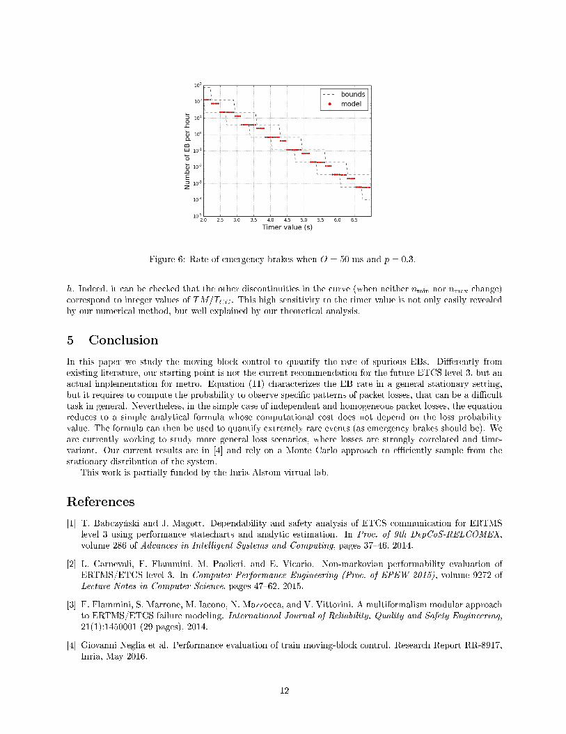
Figure 6: Rate of emergency brakes when O = 50 ms and p = 0:3.
h. Indeed, it can be checked that the other discontinuities in the curve (when neither nmin nor nmax change)correspond to integer values of TM=TCC . This high sensitivity to the timer value is not only easily revealedby our numerical method, but well explained by our theoretical analysis.
5 Conclusion
In this paper we study the moving block control to quantify the rate of spurious EBs. Di�erently fromexisting literature, our starting point is not the current recommendation for the future ETCS level 3, but anactual implementation for metro. Equation (11) characterizes the EB rate in a general stationary setting,but it requires to compute the probability to observe speci�c patterns of packet losses, that can be a di�culttask in general. Nevertheless, in the simple case of independent and homogeneous packet losses, the equationreduces to a simple analytical formula whose computational cost does not depend on the loss probabilityvalue. The formula can then be used to quantify extremely rare events (as emergency brakes should be). Weare currently working to study more general loss scenarios, where losses are strongly correlated and time-variant. Our current results are in [4] and rely on a Monte Carlo approach to e�ciently sample from thestationary distribution of the system.
This work is partially funded by the Inria-Alstom virtual lab.
References
[1] T. Babczy«ski and J. Magott. Dependability and safety analysis of ETCS communication for ERTMSlevel 3 using performance statecharts and analytic estimation. In Proc. of 9th DepCoS-RELCOMEX,volume 286 of Advances in Intelligent Systems and Computing, pages 37�46. 2014.
[2] L. Carnevali, F. Flammini, M. Paolieri, and E. Vicario. Non-markovian performability evaluation ofERTMS/ETCS level 3. In Computer Performance Engineering (Proc. of EPEW 2015), volume 9272 ofLecture Notes in Computer Science, pages 47�62. 2015.
[3] F. Flammini, S. Marrone, M. Iacono, N. Mazzocca, and V. Vittorini. A multiformalism modular approachto ERTMS/ETCS failure modeling. International Journal of Reliability, Quality and Safety Engineering,21(1):1450001 (29 pages), 2014.
[4] Giovanni Neglia et al. Performance evaluation of train moving-block control. Research Report RR-8917,Inria, May 2016.
12

[5] H. Hermanns, D. N. Jansen, and Y. S. Usenko. From StoCharts to MoDeST: A comparative reliabilityanalysis of train radio communications. In Proc. of WOSP '05, pages 13�23, 2005.
[6] A. Horváth, M. Paolieri, L. Ridi, and E. Vicario. Transient analysis of non-Markovian models usingstochastic state classes. Performance Evaluation, 69(7-8):315�335, 2012.
[7] J. Trowitzsch and A. Zimmermann. Using UML state machines and petri nets for the quantitativeinvestigation of ETCS. In Proc. of Valuetools '06, 2006.
[8] A. Zimmermann and G. Hommel. A train control system case study in model-based real time systemdesign. In Proc. of IPDPS '03, 2003.
[9] A. Zimmermann and G. Hommel. Towards modeling and evaluation of ETCS real-time communicationand operation. Journal of Systems and Software, 77(1):47�54, 2005.
13