performance comparison of tracking algorithms for...

Commun. Fac. Sci. Univ. Ank. Series A2-A3 V.51(1) pp 1-16 (2007)

PERFORMANCE COMPARISON OF TRACKING ALGORITHMS

FOR A GROUND BASED RADAR

GÖKHAN SOYSAL AND MURAT EFE

Ankara University, Faculty of Engineering, Electronics Engineering Department, 06100, Tandogan, Ankara – TURKEY E-mail: soysal,[email protected]

(Received March 22, 2007; Accepted April 09, 2007)

ABSTRACT In this paper, performance of several tracking algorithms are compared when employed in a ground based radar. The algorithms have been compared in terms of percentage track loss and rms estimation errors where the manoeuvrability of the scenarios was varied from low to moderate. 1. INTRODUCTION Phased array radars are used for ground, air or maritime surveillance and/or tracking. Electronic scanning feature of these radars provide fast and accurate beam direction. This feature helps the radar provide measurements with better accuracy which consequently improves the performance of the tracking algorithm employed. In radars, tracking algorithms are used to estimate the target states of interest (commonly position and velocity) from the noisy measurements that the radar has gathered. The fact that radar is ship based, ground based or airborne calls for caution in terms designing the tracking algorithm. For instance, if the radar of interest is ship based then special caution has to be taken to deal with heavy sea clutter. Also, performance of ground based radars is hindered by tall objects in the field of view, which in return deteriorates the tracking algorithm’s performance. However, electronic beam steering has the answer to this specific problem by allowing predetermined scanning patterns. This paper presents performance comparison of several target tracking algorithms for a ground based phased array radar. The radar is assumed to rotate mechanically, completing its 360° turn in 2 s in azimuth, while scanning electronically in elevation. Each radar return goes through a detection process and any return that


2

passes this process yileds a measurement for which the corresponding measurement errors and probability of detection (PD) are calculated. Then, the resulting measurement is fed into the tracker. The primary aim of the study is to determine the most appropriate tracking algorithm to be employed with a ground based short to mid range phased array radar. Selected tracking algorithms have been tested on selected scenarios where the targets perform mild to moderate manoeuvres at both short and mid ranges. 2. RADAR MODEL Principles of phased arrays have been applied to radars since the World War II where most of the advances in theory and technology were achieved in the 50s and the 60s. However, they came into operational use in the late 60s and the 70s. The main advantage of the phased array antennas is that the beam of the antenna can be steered electronically in a certain new direction without delay. In this study the phased array radar is modelled to scan electronically in elevation while rotating mechanically in azimuth. Also the radar is assumed to work in track and search (T&S) mode. It completes its 360° turn in 2 s during which it collects 3D (range, azimuth, elevation) measurements. The radar model is supported with realistic beam scheduling, detection and measurement units. The beam scheduling unit carries out the planning of search and track beams in accordance with T&S logic. The detection unit calculates the SNR for each hit using the predefined radar parameters, target range and target’s distance to the beam centre. The calculated SNR is then employed to yield PD which is subsequently compared with random number that is uniformly distributed between (0-1). Only radar returns whose calculated PD passes this test is declared as a valid detection. Through this test miss detection is also modelled. The measurement unit produces 3D measurements in spherical coordinates where measurements are assumed to have been taken using amplitude comparison mono pulse technique [1]. The unit computes measurements errors in elevation and azimuth (i.e., DF errors) along with the SNR which is calculated using the beam width and target’s distance to the beam centre. The DF errors are than added to the true target position in order to obtain radar measurements.


3

3. TRACKING ALGORITHMS Three different tracking algorithms, namely, probabilistic data association filter (PDAF) [2], interacting multiple model probabilistic data association filter (IMMPDAF) [2] and interacting multiple model nearest neighbour (IMMNN) algorithm, in seven different configurations have been tested on the selected scenarios. The configurations belonging to the same algorithm differ either in the number/type of models they posses or the assumption of a-priori knowledge regarding the target manoeuvre. The selected algorithms (and the configurations) are the most widely used and tested tracking algorithms in the literature. All selected algorithms are Kalman based algorithms and have been used with a data association approach to deal with clutter. 3.1 Kalman Filter Kalman filter is the traditional and most widely used state estimator [3]. The Filter is the general solution to the recursive linear minimum mean square estimation problem and it provides optimal tracking performance provided the following conditions [4] are met; i) the state of the target evolves according to a known linear dynamic model driven by a single known input and additive zero-mean, white Gaussian noise with known covariance and ii) the measurements are linear functions of the target state corrupted by additive zero-mean, white Gaussian noise with known covariance. Assuming that the target dynamic process can be modelled in discrete Markov form, then the equation that describes the target dynamics in terms of a Markov process can be written as,

( 1) ( ) ( )X k FX k V k+ = +Γ (1)

where X(k) is the k dimensional target state vector, F is the known transition matrix, Γ is the known disturbance transition matrix and V(k) is the unknown zero-mean Gaussian process noise with assumed known covariance Q. Measurements are a linear combination of the system state variables and corrupted by uncorrelated noise. Thus, the m dimensional measurement vector is modelled as

( ) ( ) ( )Z k HX k w k= + (2)

where H is the mxk measurement matrix and w(k) is zero mean, white Gaussian measurement noise with covariance R. Note that, it is assumed that V(k) and w(k) are mutually uncorrelated. A good derivation of the Kalman filter equations can be


4

found in [5], here only the resulting standard Kalman filter equations [4] are given. ˆ( 1 | ) ( | )X k k FX k k+ =% (3)

( 1) ( 1) ( 1| )v k Z k HX k k+ = + − +% (4)

( 1| ) ( | )P k k FP k k F Q′ ′+ = + Γ Γ (5)

( 1) ( 1| )S k HP k k H R′+ = + + (6)

1( 1) ( 1| ) ( 1)W k P k k H S k −′+ = + + (7)

ˆ ( 1| 1) ( 1| ) ( 1) ( 1)X k k X k k W k v k+ + = + + + +% (8)

( 1| 1) ( 1| ) ( 1) ( 1) ( 1)P k k P k k W k S k W k ′+ + = + − + + + (9)

In the Eqs (3) through (9) ( 1 | )X k k+% and P(k+1⎢k) are the predicted state and

state covariance and ˆ ( 1 | 1)X k k+ + and P(k+1⎢k+1) are the updated state and state covariance respectively. S(k+1), R, W(k+1) and ν(k+1) are the covariance of the innovation, the covariance of the measurement noise, the Kalman gain and the innovation respectively. 3.2 Interacting Multiple Model (IMM) Algorithm The Interacting Multiple Model (IMM) algorithm [4] uses a bank of filters but unlike other multiple model algorithms, it keeps the number of hypotheses fixed, which reduces the computational burden. The algorithm employs a fixed number of models that interact through state mixing to track a manoeuvring target. Every filter employed in the algorithm corresponds to a possible target motion to cover the actual modes of the target. The initial estimate at the beginning of each cycle for each filter is a mixture of all the most recent estimates from the filters. It is the mixing that enables the algorithm to effectively take the history of the modes into account. The probability of each model being true is found by using a likelihood function for the model and switching between the models is governed by a transition probability matrix. The state estimates from the sub-filters are then mixed, by means of weighting coefficients, in order to get the combined state estimate. The operation of the algorithm is completed in 4 steps; 1) Interaction of the Estimates: Mixing the state estimates for the jth model is done by using the outputs of each model

ˆ ( | )iX k k , model probability wi(k) and the transition probabilities pij .


5

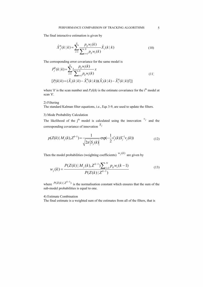
The final interactive estimation is given by

0

11

( )ˆ ˆ( | ) ( | )( )

Nij i

j iNi tj tt

p w kX k k X k k

p w k==

=∑∑

(10)

The corresponding error covariance for the same model is

0

11

0 0

( )( | ) {

( )

ˆ ˆ ˆ ˆ[ ( | ) ( ( | ) ( | ))( ( | ) ( | )) ]}

Nij i

j Ni tj tt

i i i i i

p w kP k k x

p w k

P k k X k k X k k X k k X k k

==

=

′+ − −

∑∑ (11)

where 'k' is the scan number and Pi(k|k) is the estimate covariance for the ith model at scan 'k'. 2) Filtering The standard Kalman filter equations, i.e., Eqs 3-9, are used to update the filters. 3) Mode Probability Calculation

The likelihood of the jth model is calculated using the innovation jv and the

corresponding covariance of innovation jS

1 11 1( ( ) | ( ), ) exp( ( ) ( ))22 ( )

kj j j j

j

p Z k M k Z v k S v kS kπ

− −′= −

(12)

Then the model probabilities (weighting coefficients) ( )jw k are given by

11

1

( ( ) | ( ), ) ( 1)( )

( ( ) | )

Nkj ij ii

j k

P Z k M k Z p w kw k

P Z k Z

−=

−

−= ∑

(13)

where 1( ( ) | )kP Z k Z −

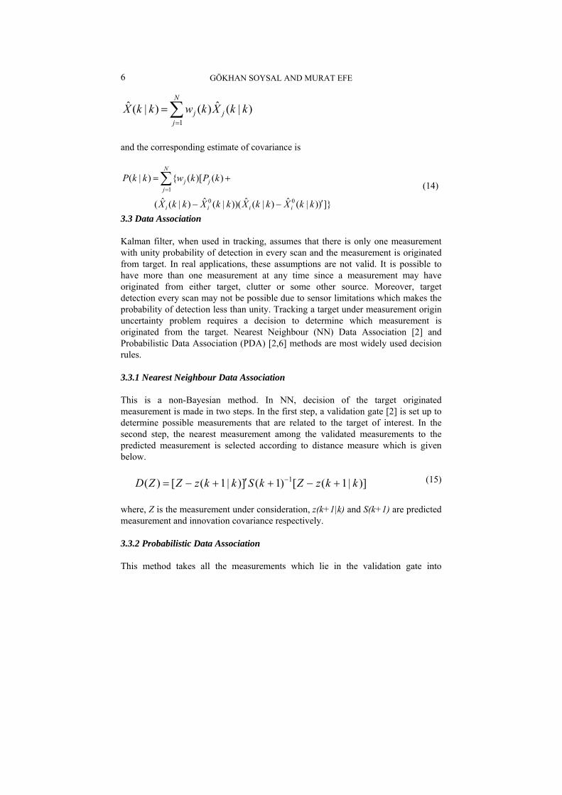
is the normalisation constant which ensures that the sum of the sub-model probabilities is equal to one. 4) Estimate Combination The final estimate is a weighted sum of the estimates from all of the filters, that is


6

1

ˆ ˆ( | ) ( ) ( | )N

j jj

X k k w k X k k=

=∑

and the corresponding estimate of covariance is

1

0 0

( | ) { ( )[ ( )

ˆ ˆ ˆ ˆ( ( | ) ( | ))( ( | ) ( | )) ]}

N

j jj

i i i i

P k k w k P k

X k k X k k X k k X k k=

= +

′− −

∑ (14)

3.3 Data Association Kalman filter, when used in tracking, assumes that there is only one measurement with unity probability of detection in every scan and the measurement is originated from target. In real applications, these assumptions are not valid. It is possible to have more than one measurement at any time since a measurement may have originated from either target, clutter or some other source. Moreover, target detection every scan may not be possible due to sensor limitations which makes the probability of detection less than unity. Tracking a target under measurement origin uncertainty problem requires a decision to determine which measurement is originated from the target. Nearest Neighbour (NN) Data Association [2] and Probabilistic Data Association (PDA) [2,6] methods are most widely used decision rules. 3.3.1 Nearest Neighbour Data Association This is a non-Bayesian method. In NN, decision of the target originated measurement is made in two steps. In the first step, a validation gate [2] is set up to determine possible measurements that are related to the target of interest. In the second step, the nearest measurement among the validated measurements to the predicted measurement is selected according to distance measure which is given below.

1( ) [ ( 1| )] ( 1) [ ( 1| )]D Z Z z k k S k Z z k k−′= − + + − + (15)

where, Z is the measurement under consideration, z(k+1|k) and S(k+1) are predicted measurement and innovation covariance respectively. 3.3.2 Probabilistic Data Association This method takes all the measurements which lie in the validation gate into


7

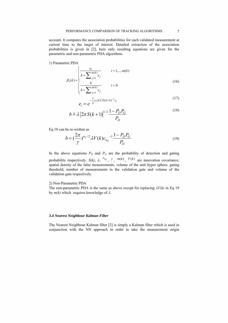
account. It computes the association probabilities for each validated measurement at current time to the target of interest. Detailed extraction of the association probabilities is given in [2], here only resulting equations are given for the parametric and non-parametric PDA algorithms. 1) Parametric PDA

( )

1

( )

1

1,..., ( )

( )0

im k

jji

m kjj

e i m kb e

kb i

b e

β=

=

⎧ =⎪+⎪

⎪= ⎨⎪ =⎪

+⎪⎩

∑

∑

(16)

11 ( ) ( 1)2 i iv k S k v

ie e−′− +

=

(17)

1/ 2 12 ( 1) D G

D

P Pb S kP

λ π−

= +% (18)

Eq 18 can be re-written as

/ 2 1 12( ) ( )ZZ

n D Gn

D

P Pb V k cP

π λγ

− −=

(19)

In the above equations PD and PG are the probability of detection and gating

probability respectively. S(k), λ, Znc, γ , ( )m k , ( )V k are innovation covariance,

spatial density of the false measurements, volume of the unit hyper sphere, gating threshold, number of measurements in the validation gate and volume of the validation gate respectively. 2) Non-Parametric PDA The non-parametric PDA is the same as above except for replacing λV(k) in Eq 19 by m(k) which requires knowledge of λ. 3.4 Nearest Neighbour Kalman Filter The Nearest Neighbour Kalman filter [2] is simply a Kalman filter which is used in conjunction with the NN approach in order to take the measurement origin


8

uncertainty into account. Integration of the Kalman filter and NN data association method is the simplest way of adapting Kalman filter to track a target under measurement origin uncertainty. NN algorithm needs to know the predicted measurement and innovation covariance which are computed by the Kalman filter. Thus, the data association unit using NN algorithm must be integrated after the computation of innovation covariance given by Eq 6. After the integration, the new filter computes state estimation and its covariance in three steps as follows: i) Compute the predicted measurement and innovation covariance in the Kalman filter manner. ii) Set up a validation gate and determine the measurements which are in the gate. iii) Select the nearest validated measurement to the predicted state using NN algorithm then update target state with this measurement, i.e., in the Kalman filter manner. 3.5.IMM-NN Filter The IMM algorithm improves tracking performance when the target manoeuvres. Thus, it is logical to employ the NN approach together with the IMM algorithm when tracking manoeuvring targets in clutter In the IMM-NN algorithm, it is essential that each filter has to update the target state using the same validated measurements, i.e., the data association unit has to set up a validation gate which is equal to the union of the mode-conditioned gates. In practice, the largest of the validations gates is approximately equal to the union and thus can be used instead. Consequently, determining the validated measurements portion of the data association procedure is performed by the filter which has the biggest validation gate in the IMM structure. This filter will be called as centre filter of the IMM-NN algorithm. The equations given for the IMM filter and the NN approach are valid for the IMM-NN algorithm. 3.6 Probabilistic Data Association Filter (PDAF) The (PDAF) is simply a Kalman filter which is used in conjunction with the PDA approach in order to take the measurement origin uncertainty into account. The filter assumes that the target is detected (perceived) and its track has been initialized. At each sampling interval a validation gate is set up and the validated measurements are determined. The measurement originating from the target of interest can be among the possible several validated measurements; hence, the track update is done by taking the weighted sum of all observations within the gated region. The weights are the association probabilities given by Eq 16 computed by the PDA algorithm. Since, more than one measurement may be used in updating the track and there is no guarantee that the target originated measurement would be amongst these measurements, state estimation update equations given by Eqs 8 and 9 its associated covariance respectively must be modified. This modification is explained in [2],


9

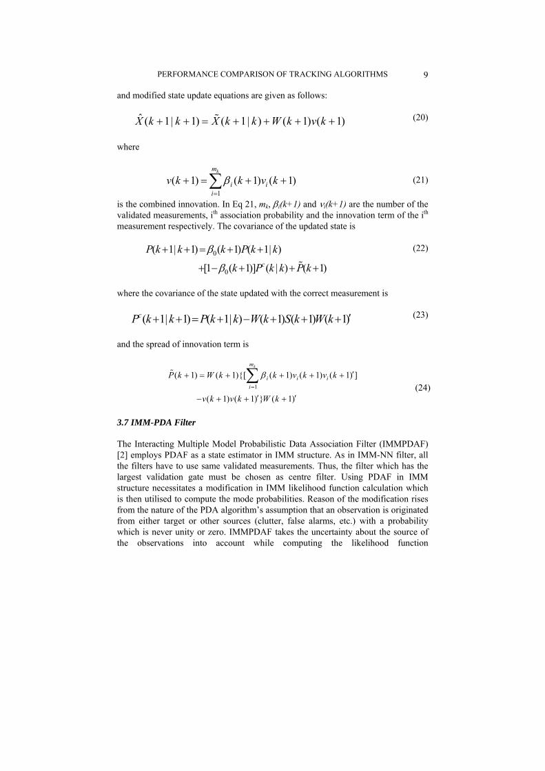
and modified state update equations are given as follows:

ˆ ( 1| 1) ( 1| ) ( 1) ( 1)X k k X k k W k v k+ + = + + + +% (20)

where

1

( 1) ( 1) ( 1)km

i ii

v k k v kβ=

+ = + +∑

(21)

is the combined innovation. In Eq 21, mk, βi(k+1) and νi(k+1) are the number of the validated measurements, ith association probability and the innovation term of the ith measurement respectively. The covariance of the updated state is

0

0

( 1| 1) ( 1) ( 1| )

[1 ( 1)] ( | ) ( 1)c

P k k k P k k

k P k k P k

β

β

+ + = + +

+ − + + +% (22)

where the covariance of the state updated with the correct measurement is

( 1| 1) ( 1| ) ( 1) ( 1) ( 1)cP k k P k k W k S k W k ′+ + = + − + + + (23)

and the spread of innovation term is

1

( 1) ( 1){[ ( 1) ( 1) ( 1) ]

( 1) ( 1) } ( 1)

km

i i ii

P k W k k v k v k

v k v k W k

β=

′+ = + + + +

′ ′− + + +

∑%

(24)

3.7 IMM-PDA Filter The Interacting Multiple Model Probabilistic Data Association Filter (IMMPDAF) [2] employs PDAF as a state estimator in IMM structure. As in IMM-NN filter, all the filters have to use same validated measurements. Thus, the filter which has the largest validation gate must be chosen as centre filter. Using PDAF in IMM structure necessitates a modification in IMM likelihood function calculation which is then utilised to compute the mode probabilities. Reason of the modification rises from the nature of the PDA algorithm’s assumption that an observation is originated from either target or other sources (clutter, false alarms, etc.) with a probability which is never unity or zero. IMMPDAF takes the uncertainty about the source of the observations into account while computing the likelihood function


10

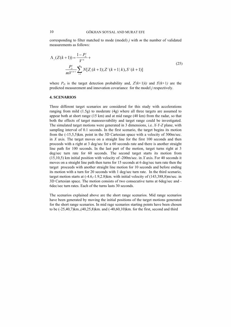
corresponding to filter matched to mode (model) j with m the number of validated measurements as follows:

where PD is the target detection probability and, Zi(k+1|k) and Si(k+1) are the predicted measurement and innovation covariance for the model j respectively. 4. SCENARIOS Three different target scenarios are considered for this study with accelerations ranging from mild (1.5g) to moderate (4g) where all three targets are assumed to appear both at short range (15 km) and at mid range (40 km) from the radar, so that both the effects of target manoeuvrability and target range could be investigated. The simulated target motions were generated in 3 dimensions, i.e. X-Y-Z plane, with sampling interval of 0.1 seconds. In the first scenario, the target begins its motion from the (-15,5,5)km. point in the 3D Cartesian space with a velocity of 300m/sec. in X axis. The target moves on a straight line for the first 100 seconds and then proceeds with a right at 3 deg/sec for a 60 seconds rate and there is another straight line path for 100 seconds. In the last part of the motion, target turns right at 3 deg/sec turn rate for 60 seconds. The second target starts its motion from (15,10,5) km initial position with velocity of -200m/sec. in X axis. For 40 seconds it moves on a straight line path then turns for 15 seconds at 6 deg/sec turn rate then the target proceeds with another straight line motion for 10 seconds and before ending its motion with a turn for 20 seconds with 1 deg/sec turn rate. In the third scenario, target motion starts at (-4.6,-1.9,2.8)km. with initial velocity of (143,388,8)m/sec. in 3D Cartesian space. The motion consists of two consecutive turns at 6deg/sec and -6dec/sec turn rates. Each of the turns lasts 30 seconds. The scenarios explained above are the short range scenarios. Mid range scenarios have been generated by moving the initial positions of the target motions generated for the short range scenarios. In mid rage scenarios starting points have been chosen to be (-25,40,7)km.,(40,25,8)km. and (-40,60,10)km. for the first, second and third

11

1( ( 1))

[ ( 1); ( 1| ), ( 1)]

jD

j m

j mj jD

imi

PZ kV

P N Z k Z k k S kmV −

=

−Λ + = +

+ + +∑

(25)


11

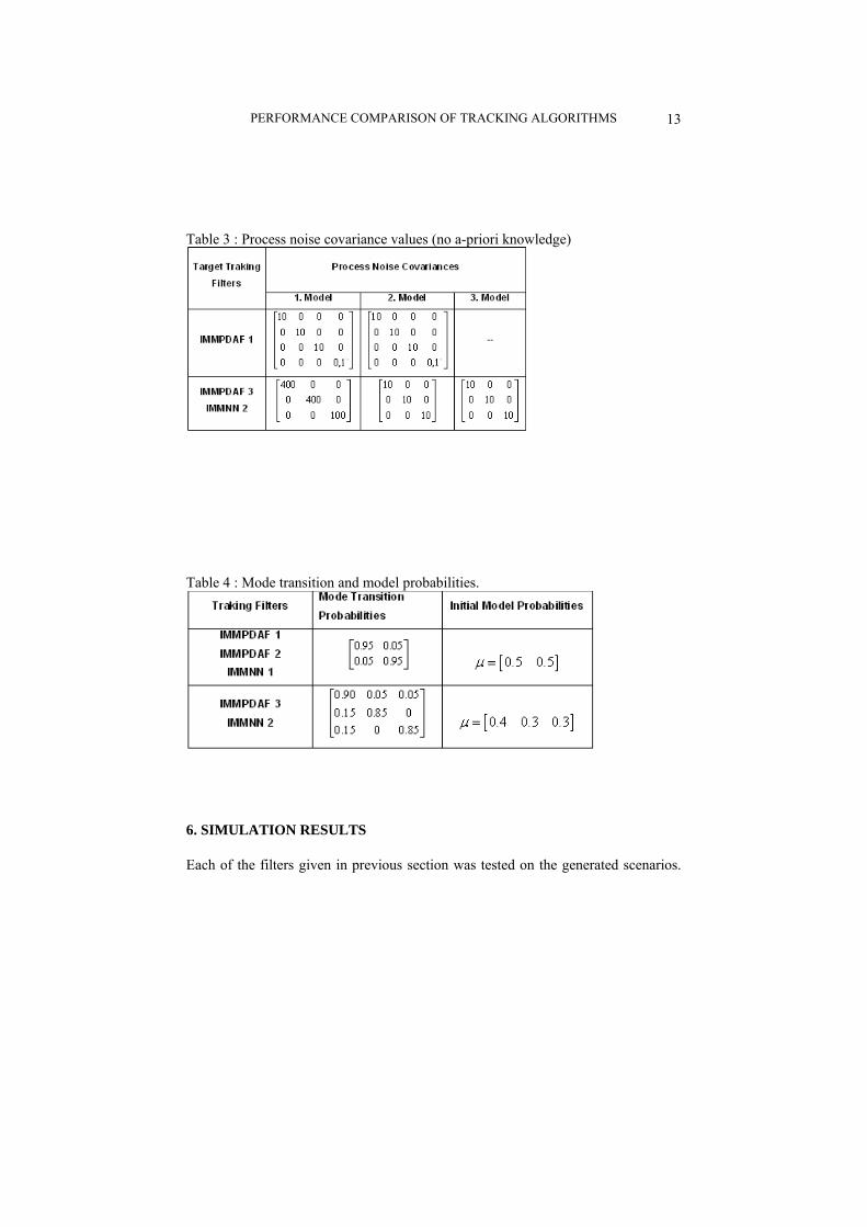
scenarios respectively. Moreover, in order to create a more realistic simulation environment for comparing the algorithms’ performance, targets are assumed to be moving in a cluttered environment where the number of clutter is assumed to have Poisson distribution and they are uniformly distributed in the surveillance region [2,6]. The Poisson parameter λ that describes the clutter density was chosen a 10-6 which corresponds to approximately 40 clutter in the chosen surveillance volume. 5. FILTERS DESIGN PARAMETERS Seven different configurations of the tracking algorithms, namely PDAF, IMMPDAF, NNKF and IMMNN, have been design to be tested on the selected scenarios. The configurations belonging to the same algorithm differ either in the number/type of models they posses or the assumption of a-priori knowledge regarding the target manoeuvre. The filters using a-priori knowledge about target manoeuvre comprise second order dynamic models. These filters are PDAF, NNKF, IMMPDAF2 and IMMNN1. The IMM algorithm based filters, i.e. IMMPDAF2 and IMMNN1, have 2 models and one of the models employs large process noise covariance to track manoeuvres where the second one utilises small process noise covariance to track benign motion. Process noise covariance of the PDAF and NNKF approaches has been selected sufficient enough to track the maximum acceleration change. Tables 1 and 2 present process noise covariance values selected for the first two scenarios whereas process noise covariance values used for the third scenario where the target performs a bigger manoeuvre are shown in Table 3. Other IMM based filters, namely IMMPDAF1, IMMPDAf3, IMMNN2, have been designed to track a target without a-priori knowledge regarding the target manoeuvre. IMMPDAF1 algorithm includes two second order models (a coordinated turn model in XY plane and a linear model). Three model IMM structure has been used in IMMPDAF3 and IMMNN2 filters. Dynamic models employed in three model IMM structures are; Model 1: Third order dynamic model with large process noise covariance for tracking onset or end of acceleration. Model 2: Third order dynamic model with small process noise covariance for tracking nearly constant acceleration motion. Model 3: Second order dynamic model with small process noise covariance for tracking nearly constant velocity motion.


12

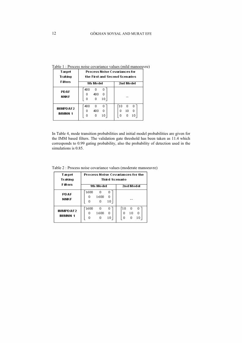
Table 1 : Process noise covariance values (mild manoeuvre)

In Table 4, mode transition probabilities and initial model probabilities are given for the IMM based filters. The validation gate threshold has been taken as 11.4 which corresponds to 0.99 gating probability, also the probability of detection used in the simulations is 0.85. Table 2 : Process noise covariance values (moderate manoeuvre)


13

Table 3 : Process noise covariance values (no a-priori knowledge)

Table 4 : Mode transition and model probabilities.

6. SIMULATION RESULTS Each of the filters given in previous section was tested on the generated scenarios.


14

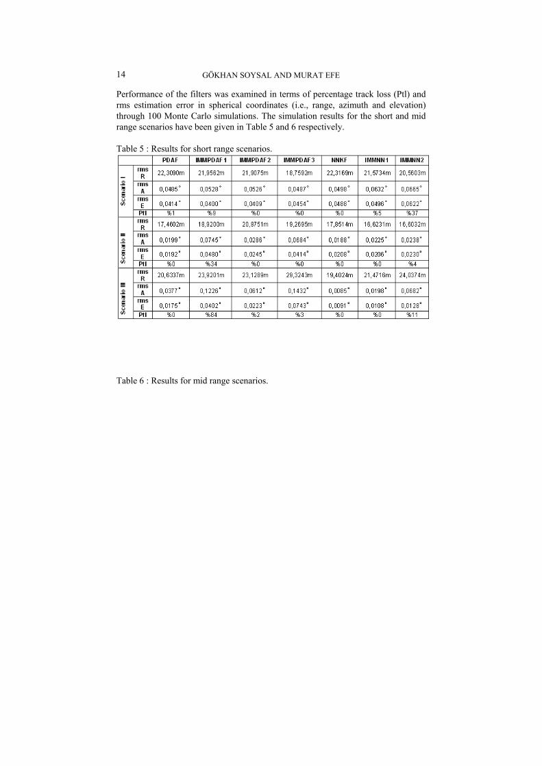
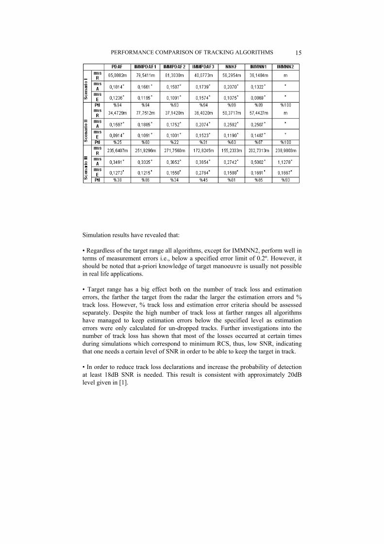
Performance of the filters was examined in terms of percentage track loss (Ptl) and rms estimation error in spherical coordinates (i.e., range, azimuth and elevation) through 100 Monte Carlo simulations. The simulation results for the short and mid range scenarios have been given in Table 5 and 6 respectively. Table 5 : Results for short range scenarios.

Table 6 : Results for mid range scenarios.


15

Simulation results have revealed that: • Regardless of the target range all algorithms, except for IMMNN2, perform well in terms of measurement errors i.e., below a specified error limit of 0.2º. However, it should be noted that a-priori knowledge of target manoeuvre is usually not possible in real life applications. • Target range has a big effect both on the number of track loss and estimation errors, the farther the target from the radar the larger the estimation errors and % track loss. However, % track loss and estimation error criteria should be assessed separately. Despite the high number of track loss at farther ranges all algorithms have managed to keep estimation errors below the specified level as estimation errors were only calculated for un-dropped tracks. Further investigations into the number of track loss has shown that most of the losses occurred at certain times during simulations which correspond to minimum RCS, thus, low SNR, indicating that one needs a certain level of SNR in order to be able to keep the target in track. • In order to reduce track loss declarations and increase the probability of detection at least 18dB SNR is needed. This result is consistent with approximately 20dB level given in [1].


16

• IMMNN approach has not produced a stable performance. The filter tends to diverge following relatively large estimation errors; due to its weighted structure IMMPDA approach is more robust in such cases. Thus it is recommended that IMM and NN approaches not be employed together. • Three dimensional nonlinear target models (i.e., a coordinated turn model in XY plane and a 2nd degree model in Z used in IMMPDAF1) cause filter divergence, thus, degraded tracking performance and they are not recommended. • The three model IMMPDA approach with no a-priori knowledge regarding the target motion has compared well with algorithms that, unrealistically, assumed knowledge of target manoeuvre and proved to be a successful tracking algorithm for ground based radar both at short and mid ranges. 7. CONCLUSIONS Performance of most commonly used tracking algorithms has been compared for ground based radar. Algorithms have been compared in terms of track loss and rms estimation errors. The 3 model IMMPDAF algorithm with no a-priori knowledge of the target motion has compared favourably with all the tested algorithms even with the ones that assume knowledge of the target manoeuvre. ÖZET Bu makalede kara konuşlu bir radar için çeşitli hedef takibi algorimalarının performansları karşılaştırılmıştır. Algoritma performans ölçüsü olarak yüzde iz kaybı ve ortalama karekök hata esas alınmıştır. Algoritmaların performansı manevra seviyesi düşükten orta seviyeye değişen hedef senaryoları üzerinde incelenmiştir. REFERENCES [1] M. I. Skolnik. “Radar Handbook”, McGraw-Hill, Inc . [2] Bar-Shalom Y., Li X. R., ”Mulltitarget–Multisensor Tracking: Principles

and Techniques.”, YBS Publishing, 1995.


17

[3] Kalman R. E., ”A New Approach to Linear Filtering and Prediction

Problems.”, Journal of Basic Engineering, Vol 82, No 1, pp 35 – 46, 1960. [4] Y. Bar Shalom, X. R. Li, T. Kirubarajan0, “Estimation with Applications

to Tracking and Navigation”, Wiley,2002. [5] Gelb, A.,” Applied Optimal Estimation”, MIT Press, 1974. [6] S. S. Blackman., “Design and Analysis of Modern Tracking Systems”,

Artech House, Norwood, MA, 1999.

performance comparison of tracking algorithms for...

Documents