Performance Analysis of Cellular Networks with Digital Fixed Relays

By

Huining Hu, B.Eng.

A thesis submitted to

The Faculty of Graduate Studies and Research

In partial fulfillment of

The requirements of the degree of

Master of Applied Science

Ottawa-Carleton Institute for Electrical and Computer Engineering

Department of Systems and Computer Engineering

Carleton University

Ottawa, Ontario

© Copyright 2003, Huining Hu

The undersigned hereby recommends to the Faculty of Graduate Studies and Researchacceptance of the thesis

Performance Analysis of Cellular Networks with Digital Fixed Relays

Submitted by Huining Hu

In partial fulfillment of the requirements for the

Degree of Master of Applied Science

_____________________________Thesis Supervisor

Dr. Halim Yanikomeroglu

___________________________________________________Chair, Department of Systems and Computer Engineering

Dr. Rafik A. Goubran

Carleton UniversitySeptember 2003

iii

Abstract

The concept of relaying is a promising solution for the challenging throughput and

high data rate coverage requirements of future wireless cellular networks. In this thesis

we demonstrate that throughput and high data rate coverage can be enhanced

significantly in such networks through the use of digital fixed relays operating with rather

straightforward protocols which do not incur any capacity penalty (except for some

modest signalling overhead); this demonstration is the main contribution of this thesis.

In particular we considered the downlink of a non-CDMA network where 6 digital

fixed relays are placed evenly in each cell in a hexagonal layout. A user equipment

chooses to receive the transmitted signal either directly (in single hop) from the base

station or via one of the relays (in two hops). Distance-, pathloss-, and SINR-based

algorithms are studied for the relay selection process. Whenever a relay is used, a second

channel is needed as the relays cannot receive and transmit at the same channel. We

propose a "pre-configured" relaying channel selection algorithm in which relays further

reuse the already used channels in the network; but this reusing is done in a controlled

manner in order to prevent the co-channel interference increasing to unacceptable levels.

Due to the "pre-configured" nature of this algorithm, the channel selection is fixed

(i.e., not dynamic) which incurs minimal overhead; at the same time, the benefits of

relaying are achieved without any need for additional bandwidth. The improved links are

exploited to yield higher throughput through the use of adaptive modulation and coding.

Diversity benefits are also studied whenever the signal is received in two-hops.

We investigated the performance of the proposed algorithms for a number of system

variables, including propagation parameters, cell sizes, transmit power levels, relay

locations, number of user equipments, and transmission bandwidth, through Monte-Carlo

simulations. We consistently observed that the throughput is increased and the outage is

decreased (which may be converted to range extension), without any capacity penalty, for

the realistic range of values of the parameters investigated. Our overall conclusion is that

digital fixed relaying has great potential in providing the envisioned high data rate

coverage in future wireless cellular networks.

iv

Acknowledgments

First and most importantly of all, I would like to express my sincerest appreciation to

my thesis supervisor, Dr. Halim Yanikomeroglu, for the tremendous time, comprehensive

guidance and consistent support he has provided for this research. His profound

knowledge and strong interests in this research area, as well as his nice personality have

been an impetus to the completion of my study. I feel very proud and very honoured to

have him as my thesis supervisor.

Secondly, I am grateful to Dr. David Falconer, as he has taken time to offer me

academic support ever since the beginning of this research. My many thanks are extended

to my academic advisor, Dr. Ian Marsland, as he has given me kind advice on course

selections. I would also like to thank Xiaobin Tang, a member of this research team, in

discussing and comparing her research results with mine.

In addition, I would like to take this opportunity to thank Nortel Networks for their

financial support to make this research a success. Especially, I thank Dr. Shalini

Periyalwar of Nortel Networks for many of her kind recommendations.

Last but not least, my family’s support is another catalyst in my research motivation. I

bestow my special gratitude upon my parents, my husband and my lovely daughter.

v

Table of Contents

Abstract ……………………………………………………………………………….. iii

Acknowledgments …………………………………………………………………….. iv

Table of Contents ……………………………………………………………………… v

List of Figures and Tables …………………………………………………………... viii

List of Acronyms …………………………………………………………………….. xiii

List of Symbols ……………………………………………………………………….. xiv

Chapter 1 - INTRODUCTION ………………………………………………………... 1

1.1 Nortel Networks Project on Cellular Networks with Relaying …………………. 2

1.2 Thesis Motivation ……………………………………………………………….. 4

1.3 Research Overview ……………………………………………………………… 7

1.4 Relevant Literature ………………………………………………………………. 9

1.5 Thesis Organization ……………………………………………………………. 10

Chapter 2 - RELAYING CHANNEL PARTITION SCHEME AND RELAY SELECTION …………………………………………………………….. 12

2.1 Propagation Model ………………………………………………………………12

2.2 Adaptive Modulation and Coding …………………………………………...….13

2.3 Cellular Layout …………………………………………………………………17

2.4 Relaying Channel Partition Scheme …………………………………………….20

2.5 Relay Selection ………………………………………………………………….27

2.5.1 Distance-based Algorithm ……………………………………………………… 28

2.5.2 Pathloss-based Algorithm ……………………………………………………… 30

2.5.3 SINR-based Algorithm ……………………………………………………………31

vi

2.6 Diversity … … … … … … … … … … … … … … … … … … … … … … … … … … … … 32

2.7 Simulation Model for N = 1 Case … … … … … … … … … … … … … … … … … … .33

Chapter 3 - SIMULATION ALGORITHM … … … … … … … … … … … … … … … … 34

3.1 Environment and Parameters Assumptions … … … … … … … … … … … … … … . 34

3.2 Simulation Algorithm for N = 4 Case … … … … … … … … … … … … … … … … .. 35

3.3 Simulation Algorithm for N = 1 Case … … … … … … … … … … … … … … … … .. 41

Chapter 4 - SIMULATION RESULTS, PART I: N = 4 CASE … … … … … … … … . 44

4.1 Average Spectral Efficiency for SINR-based Algorithm … … … … … … … … … .44

4.2 Relay Usage … … … … … … … … … … … … … … … … … … … … … … … … … … ..46

4.3 Average Spectral Efficiency for with and without ORB Cases … … … … … … … 48

4.4 Average Spectral Efficiency Comparison for Different Relay Selection Algorithms … … … … … … … … … … … … … … … … … … … … … … … … … … … 51

4.5 Average Spectral Efficiency Comparison for with and without Diversity … … .. 53

4.6 Effect of Background Noise … … … … … … … … … … … … … … … … … … … … . 55

4.7 Effect of Bandwidth (i.e., Noise Power) … … … … … … … … … … … … … … … .. 56

4.8 Effect of Pathloss Exponent … … … … … … … … … … … … … … … … … … … … ..57

4.9 Adaptive Modulation and Coding Histograms … … … … … … … … … … … … … .60

4.10 Coverage Extension … … … … … … … … … … .… … … … … … … … … … … … ...64

Chapter 5 - SIMULATION RESULTS, PART II: N = 1 CASE … … … … … … … .. 67

5.1 Average Spectral Efficiency with respect to Interference Suppression Factor … … … … … … … … … … … … … … … … … … … … … … … … … … … … … 67

5.2 Coverage at Various SINR Levels with respect to Interference Suppression Factor … … … … … … … … … … … … … … … … … … … … … … … … … … … … … 69

5.3 Average Spectral Efficiency with respect to Relay Positions … … … … … … … .. 71

5.4 Coverage Extension … … … … … … … … … … .… … … … … … … … … … … … .… 74

vii

Chapter 6 – CONCLUSIONS AND DISCUSSIONS...… … … … … … … … … … … … .76

6.1 Conclusions … … … … … … … … … … … … … … … … … … … … … … … … … … .. 76

6.2 Thesis Contributions … … … … … … … … … … … … … … … … … … … … … … … .77

6.3 Future Research … … … … … … … … … … … … … … … … … … … … … … … … … 78

References … … … … … … … … … … … … … … … … … … … … … … … … … … … … … … 80

Appendix A - Geometric Characteristic of Co-channel BSs and Relays for Cluster Size N = 3 and N = 7 Cases … … … … … … … … … … … … … … 84

Appendix B - Proof of “the locus is a circle when meeting the condition the ratio of the distances of a moving point to two fixed points is a constant” … … … … … … … … … … … … … … … … … … … … … … … . 86

Appendix C - Diversity Results for Cluster Size N = 4 and N = 1 Cases… … … … … 92

viii

List of Figures and Tables

Figure 2.1 BER vs. SINR for combinations of various modulations and code rates… … … … … … … … … … … … … … … ...… … … … … .… … … ...15

Table 1 Relation of all combinations, required SINR and spectral efficiency that will yield BER of 10-5 … … … … … … … … … … … … … … ..… … … … … … .16

Figure 2.2 BS and relay positions… … … … … … … … … … … … … … … … … … … … … .17

Figure 2.3 Cellular layout (N = 4)… … … .… … … … … … … … … … … … … … … … … … 18

Figure 2.4 Evenly distributed BSs and relays without cell boundaries (N = 4)… … … … 19

Figure 2.5 One relay reusing a channel from cell D… … … … … … … … … … .… … … … 22

Figure 2.6 All relays reusing channels from cell D… … … … … … ...… … … … … … … ...23

Figure 2.7 Cell layout and relaying channel partition scheme… … … … … ...… … … … ...24

Figure 2.8 Geometric characteristic of co-channel BSs and relays (N = 4)… … … … … ..25

Figure 2.9 BS & relay coverage boundary in distance-based algorithm… … … … … … ..29

Figure 2.10 Simplified BS & relay coverage boundary in distance-based algorithm… … … … … … … … … ..… … … … … … … … … … … … … … … … . 30

Figure 2.11 Pathloss- and SINR-based algorithms… … … ...… … … … … … … … … … … 31

Figure 2.12 Diversity algorithm… … … … … … … … … … … … … … … … … … … … … ... 32

Figure 2.13 Cellular layout for cluster size N = 1 case… … … … … … … … … … .… … ... 33

Figure 3.1 Interference received by UE 2 from other BSs and relays (When UE 2 receives signal from the BS)… … … … … … ...… … … … … … ... 38

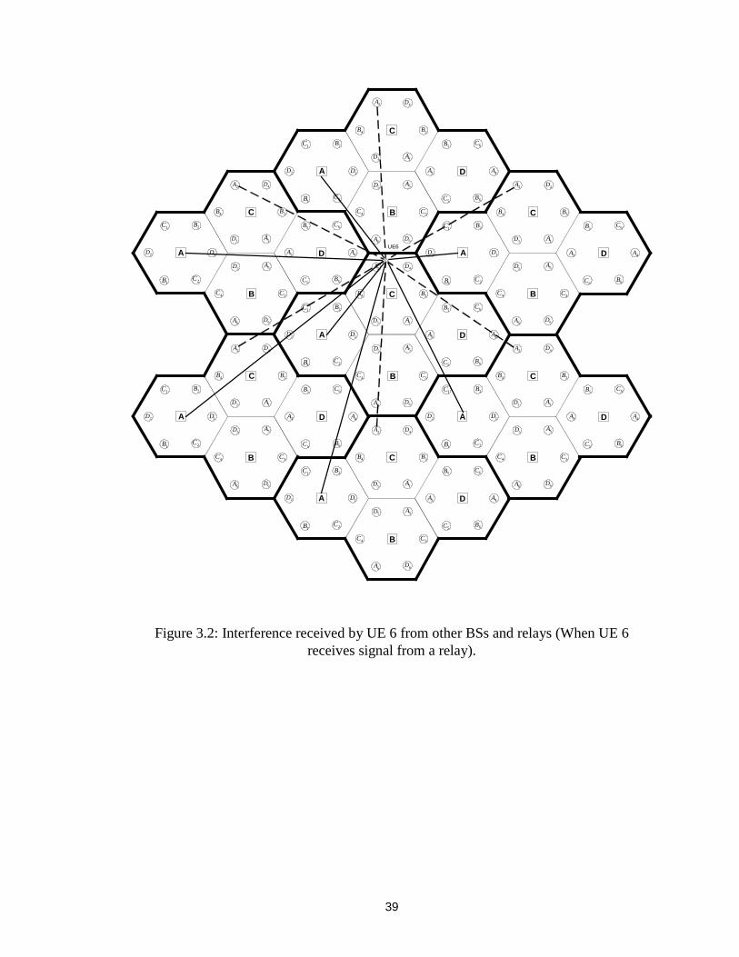
Figure 3.2 Interference received by UE 6 from other BSs and relays (When UE 6 receives signal from a relay)… … … … … … … … … … … … … .. 39

Figure 3.3 Flowchart (when ORB is not taken into account)… … … … ...… … … … … … 40

Figure 3.4 Flowchart (when ORB is taken into account)… … … … … … … … … … … … .41

ix

Figure 3.5 Interference sources for cluster size N = 1 case (when UE receives signal from a relay)… … … … … … … … … … … … … … ...… … … … … … … … … … . 42

Figure 3.6 Interference sources for cluster size N = 1 case (when UE is receives signal from the BS)… … … … … … … … … ...… … … … … … … … … … … … … .… … 43

Figure 4.1 Average spectral efficiency (SINR-based relay selection algorithm, R = 2000 m, N = 4)… … … … … … … … … … … … … … … … … … … … … … . 45

Figure 4.2 Average spectral efficiency (SINR-based relay selection algorithm, R = 1000 m, N = 4)… … … … … … … … … ...… … … … … … … … … .… … … . 45

Figure 4.3 Average spectral efficiency (SINR-based relay selection algorithm, R = 500 m, N = 4)… … … … … … … … … … … … … … … … … … … … … … … 46

Figure 4.4 Percentage of users affected by ORB (SINR-based relay selection algorithm, N = 4)… … … … … … … … … … … ...… … … … … … … … … … … .. 47

Figure 4.5 Percentage of users communicating with relays (SINR-based relay selection algorithm, N = 4)… … … … … … … … … ...… … … … … … … . 48

Figure 4.6 Average spectral efficiency comparison for two cases: with and without ORB incorporated (SINR-based relay selection algorithm, R = 2000 m, N = 4)… … … … … … … … … … … … … … … … … … 49

Figure 4.7 Average spectral efficiency comparison for two cases: with and without ORB incorporated (SINR-based relay selection algorithm, R = 1000 m, N = 4)… … … … … … … … … … … … … … … … … … 50

Figure 4.8 Average spectral efficiency comparison for two cases: with and without ORB incorporated (SINR-based relay selection algorithm, R = 500 m, N = 4)… … … … … … … … … … … … … … … … … … ..50

Figure 4.9 Average spectral efficiency comparison for distance-, pathloss- and SINR-based relay selection algorithms (R = 2000 m, N = 4)… … … … … … ..51

Figure 4.10 Average spectral efficiency comparison for distance-, pathloss- and SINR-based relay selection algorithms (R = 1000 m, N = 4)… … … … … ....52

Figure 4.11 Average spectral efficiency comparison for distance-, pathloss- and SINR-based relay selection algorithms (R = 500 m, N = 4)… … … … … ......52

Figure 4.12 Average spectral efficiency comparison for with and without diversity (SINR-based relay selection algorithm, R = 2000 m, N = 4)… … … … … .… 53

Figure 4.13 Average spectral efficiency comparison for with and without diversity

x

(SINR-based relay selection algorithm, R = 1000 m, N = 4)… … … … ..… .54

Figure 4.14 Average spectral efficiency comparison for with and without diversity (SINR-based relay selection algorithm, R = 500 m, N = 4)… … … … … … ..54

Figure 4.15 Average spectral efficiency comparison for with and without background noise (SINR-based relay selection algorithm, R = 1000 m, N = 4)… … … … … … … … … … … … … … … … … … … … … … 55

Figure 4.16 Average spectral efficiency for different bandwidth values (SINR-based relay selection algorithm, Prel = 1 W, R = 1000 m, N = 4)… … … … … … … … … … … … … … … … … … … … … … 56

Figure 4.17 Average spectral efficiency for different propagation exponent (n) values (SINR-based relay selection algorithm, Prel = 1 W, R = 2000 m, N = 4)… … … … … … … … … … … … ...… … … … … … … … … .58

Figure 4.18 Average spectral efficiency for different propagation exponent (n) values (SINR-based relay selection algorithm, Prel = 1 W, R = 1000 m, N = 4)… … … … … … … … … … … … ...… … … … … … … … … .59

Figure 4.19 Average spectral efficiency for different propagation exponent (n) values (SINR-based relay selection algorithm, Prel = 1 W, R = 500 m, N = 4)… … … … … … … … … … … … ...… … … … … … … … ..… .59

Table 2 Coverage results… … … … … … … … … … … … … … … … .… … … … … … … … ..60

Table 3 Outage results… … … … … … … … … … … … … … … … … .… … … … … … … … ..61

Figure 4.20 Percentage of time using a combination of modulation and coding (without relaying, SINR-based relay selection algorithm, R = 2000 m, N = 4)… … … … … … … … ...… … … … … … … … … … .… … … 61

Figure 4.21 Percentage of time using a combination of modulation and coding (with relaying, Prel = 1 W, SINR-based relay selection algorithm, R = 2000 m, N = 4)… … … … … … … … … … … … … … … … … … … … … … 62

Figure 4.22 Percentage of time using a combination of modulation and coding (without relaying, SINR-based relay selection algorithm, R = 1000 m, N = 4)… … … … … … … … … … … … … … … … … … … … … … 62

Figure 4.23 Percentage of time using a combination of modulation and coding (with relaying, Prel = 1 W, SINR-based relay selection algorithm, R = 1000 m, N = 4)… … … … … … … … … … … … … … … … … … … … … … 63

Figure 4.24 Percentage of time using a combination of modulation and coding

xi

(without relaying, SINR-based relay selection algorithm, R = 500 m, N = 4)… … … … … … … … … … … … … … … … … … … … … … ..63

Figure 4.25 Percentage of time using a combination of modulation and coding (with relaying, Prel = 1 W, SINR-based relay selection algorithm, R = 500 m, N = 4)… … … … … … … … … … … … … … … … … … … … … … ..64

Figure 4.26 Average spectral efficiency for different cell sizes (SINR-based relay selection algorithm, Prel = 1 W, N = 4)… … … … … … … … … … … … … … ..65

Figure 4.27 Outage results for different cell sizes (SINR-based relay selection algorithm, Prel = 1 W, N = 4)… … … … … … … … … … … … … … ..66

Figure 5.1 Average spectral efficiency with respect to interference suppression factor (SINR-based algorithm, Prel = 1 W, R = 2000 m, N = 1, no diversity)… … … … … … … … … ...… … … … … … … … … … … … ..68

Figure 5.2 Average spectral efficiency with respect to interference suppression factor (SINR-based algorithm, Prel = 1 W, R = 1000 m, N = 1, no diversity)… … … … … … … … … ...… … … … … … … … … … … … ..68

Figure 5.3 Average spectral efficiency with respect to interference suppression factor (SINR-based algorithm, Prel = 1 W, R = 500 m, N = 1, no diversity)… … … … … … … … … … … … … … … … … … … … … … .69

Figure 5.4 Coverage at various SINR levels with respect to interference suppression factor (SINR-based algorithm, Prel = 1 W, R = 2000 m, N = 1, no diversity)… … … … … … … … … … … … … … … … … … … … … … .70

Figure 5.5 Coverage at various SINR levels with respect to interference suppression factor (SINR-based algorithm, Prel = 1 W, R = 1000 m, N = 1, no diversity)… … … … … … … … … … … … … … … … … … … … … … .70

Figure 5.6 Coverage at various SINR levels with respect to interference suppression factor (SINR-based algorithm, Prel = 1 W, R = 500 m, N = 1, no diversity)… … … … … … … … … … … … … … ...… … … … … … … ...71

Figure 5.7 Relay position… … … … … … … … … … … … … … … … … … … … .… … … … .72

Figure 5.8 Average spectral efficiency with respect to relay positions (SINR-based relay selection algorithm, with relay, Prel = 1 W, N = 1, ISF = 0.2) … … … ...72

Figure 5.9 Percentage of users affected by Optimal-Route-Blockage (SINR-based relay selection algorithm, R = 1000 m, ISF = 0.2, Prel = 1 W, N = 1) … … ....73

Figure 5.10 Percentage of users communicating with relays (SINR-based

xii

relay selection algorithm, R = 1000 m, ISF = 0.2, Prel = 1 W, N = 1)… … … .74

Figure 5.11 Average spectral efficiency for different cell sizes (SINR-based relay selection algorithm, Prel = 1 W, N = 1)… … … … … … … … … … … … … … ..75

Figure 5.12 Outage results for different cell sizes (SINR-based relay selection algorithm, Prel = 1 W, N = 1)… … … … … … … … … … … … … … ..75

Figure A.1 Cluster size N = 3 case… … … … … … … … … … … … … … … … … … … … … 84

Figure A.2 Cluster size N = 7 case… … … … … … … … … … … … … … … … … … … … … 85

Table B.1 Locus information based on various relP values (R = 1000 m) … … … … … ..88

Figure B.1 Distance-based relay selection in various relay transmit power settings, R = 1000 m… … … … … … … … … … … … … … … ..90

Figure B.1 Distance-based relay selection in various relay transmit power settings, R = 1000 m (Continued)… … … … … … … … … … ..91

Figure C.1 Percentage of time using a combination of modulation and coding (with relaying, Prel = 1 W, SINR-based relay selection algorithm, with diversity, R = 2000 m, N = 4)… … … … … … … … … … … … … … … … 92

Figure C.2 Percentage of time using a combination of modulation and coding (with relaying, Prel = 1 W, SINR-based relay selection algorithm, with diversity, R = 1000 m, N = 4)… … … … … … … … … … … … … … … … 93

Figure C.3 Percentage of time using a combination of modulation and coding (with relaying, Prel = 1 W, SINR-based relay selection algorithm, with diversity, R = 500 m, N = 4)… … … … … … … … … … … … … … … … ..93

Figure C.4 Coverage at various SINR levels with respect to interference suppression factor (SINR-based algorithm, Prel = 1 W, R = 2000 m, N = 1, with diversity)… … … … … … … ..… … … … … … … … … … … … … … … … ..94

Figure C.5 Coverage at various SINR levels with respect to interference suppression factor (SINR-based algorithm, Prel = 1 W, R = 1000 m, N = 1, with diversity)… … … … … … … ..… … … … … … … … … … … … … … … … ..94

Figure C.6 Coverage at various SINR levels with respect to interference suppression factor (SINR-based algorithm, Prel = 1 W, R = 500 m, N = 1, with diversity)… … … … … … … ..… … … … … … … … … … … … … … … … ..95

xiii

List of Acronyms

AMC Adaptive Modulation and Coding

AWGN Additive White Gaussian Noise

BER Bit Error Rate

BICM Bit-Interleaved Coded Modulation

BS Base Station

CDMA Code Division Multiple Access

EIRP Effective Isotropic Radiated Power

GPS Global Positioning System

LOS Line-of-Sight

MIMO Multi-Input-Multi-Output

MRC Maximal Ratio Combining

OFDM Orthogonal Frequency Division Multiplexing

ORB Optimal Route Blockage

QAM Quadrature Amplitude Modulation

QPSK Quadrature Phase Shift Keying

SINR Signal to Interference and Noise Ratio

TDMA Time Division Multiple Access

UE User Equipment

WLAN Wireless Local Area Network

xiv

List of Symbols

a Distance between BS and relay

c Speed of light

d Distance between transmitter and receiver

d0 Reference distance

d1 Distance between BS and UE

d2 Distance between relay and UE

f Carrier frequency

F Noise figure

Gr Antenna gain of receiver

Gt Antenna gain of transmitter

ISF Interference suppression factor

k Constant

Kb Boltzmann’s constant

m Distance ratio of BS to relay and BS to one corner of cell

n Propagation exponent

ns Selected node (BS or relay) for transmitting signals to UE

N Cluster size

PBS BS transmit power

PI Received interference power

PN Received noise power

Pr Received power

xv

Pr1 Received signal power at UE from BS

Pr2 Received signal power at UE from relay

Prel Relay transmit power

PS Received signal power

Pt Transmitted power

PL Average pathloss

PLBS Pathloss between BS and UE

PLR1 Pathloss between relay 1 and UE

PLR2 Pathloss between relay 2 and UE

R Cell radius

S Number of UEs per cell

SINRBS SINR received at UE from BS

SINRR1 SINR received at UE from relay 1

SINRR2 SINR received at UE from relay 2

T System temperature

W Transmission bandwidth

X1, X2 Two independent Gaussian random variables

X � A lognormally distributed random variable with stand deviation σ

Y An exponential random variable

β Pathloss adjustment coefficient

1

Chapter 1 Introduction

Modern cellular networks not only need to provide high quality voice for customers,

but a large amount of data transfer service as well, such as wireless internet, multimedia,

file transfer and downloading. These concerns lead to the new demand to enhance the

throughput and high data rate coverage for future cellular networks. However,

conventional cellular networks cannot offer the Signal to Interference and Noise Ratio

(SINR) that is high enough to meet the new requests. Theoretical difficulties will be

encountered if the future 4G networks are constructed purely based on conventional

network architecture. First, the transmission rate for the future 4G networks is much

higher than that of 3G networks, which will adversely affect the SINR at the receiving

end, since SINR is in inverse proportion to the transmission rate∗. Second, the spectrum

allocated for 4G networks could be well above 2 GHz used by 3G networks. Under the

operation of such a high band, the received signal will decrease tremendously according

to the radio propagation model detailed in Section 2.1 and formulas (1) and (2) [5, 29].

We can resort to applying interference cancellation algorithms or smart antenna

technologies, such as MIMO or adaptive antennas to distribute and collect signals more

efficiently, but these technologies can only solve the problem to a certain extent, since

even the most advanced antenna does not work well with the existence of heavy

shadowing in the network, plus applying complicated antenna techniques on UEs may be

unrealistic [5].

∗ When the transmit power is a constant, and if the transmit rate increases, then the bit energy Eb decreases.Since noise spectral density N0 is a constant, Eb/N0 decreases, so SINR decreases.

2

Another way to get stronger SINR values at the receiving end is to shorten the

communication links between the BS and UEs. Employing more BSs can lead to shorter

communication links. Pico-cell or micro-cell infrastructures are examples of denser BS

deployment. However, none of these are ideal solutions due to the high deployment costs.

A novel solution to shorten the communication links is multi-hop or relaying

technology. This is a cost effective approach since relays are functionally much simpler

than BSs, which is explained in Section 1.2. The concept of relaying is that “relays” are

new network elements in a cell and they act as the intermediate signal forwarding points

between the BS and UEs. Their signal relaying mechanism is two-way: from BS to UE

and from UE to BS. This greatly aids the signal transmission between the BS and UEs

and guarantees stronger and more stable receiving signals, especially for the UEs near the

edge of the cell, thereby improving the overall system throughput.

1.1 Nortel Networks Project on Cellular Networks with Relaying

Today’s cellular mobile networks are mainly “single hop”, meaning there is only one

hop involved for a BS and a UE to exchange information. Some cellular networks use

analog repeaters to provide service to coverage holes (such as subway stations). Lately,

the potential of cellular multi-hop networks in the provision of ubiquitous high data rate

coverage has been discovered, and currently there is great interest on this concept both in

academia and in industry [1,2,3].

This entire Nortel Networks-funded research studies from various perspectives how

multi-hop relaying technology can improve system throughput and high date rate

coverage in cellular networks. It is an on-going research and is carried out in phases.

3

The research work in Phase I concerns digital peer-to-peer relaying [4, 8, 29-31],

which is summarized in this paragraph. In peer-to-peer relaying, any UE with adequate

received signals from the BS can relay signals for other UEs with poor received signals

from the BS. In that research, relaying channels (for relays to forward signals to UEs) are

acquired via reusing already used channels in the neighboring cells in the same cluster. A

loaded cellular TDMA system with square cells and omni-directional antennas is

considered as the network environment. More specifically, two types of systems, noise-

limited and interference-limited systems, are investigated. In an attempt to have better

radio resource management, multiple relay selection schemes, relaying channel selection

schemes and relaying power selection and control schemes are studied. Overall, the

simulation results show that better performance returns can be achieved through this type

of mobile digital relaying, as opposed to the without-relaying scenario. Peer-to-peer

relaying is able to provide better performance results when the number of UEs in a cell

increases. Moreover, a network with peer-to-peer relaying is quite sensitive to relay

selection scheme, but insensitive to relaying channel selection scheme. Different relay

selection criteria can make a big difference on system performance; on the contrary, the

performance differences among relaying channel selection criteria are not significant

provided that the relays are selected appropriately. Additionally, the simulations indicate

that power control can further enhance the performance returns, especially for small-size

cells. In large cells, a better system performance can be achieved with higher relay

transmit power levels; in small cells, on the other hand, most of the performance returns

can be achieved with relatively low relay transmit power levels. One important

4

conclusion of Phase I research suggested that peer-to-peer relaying can be realized

without much stress on the batteries of the UEs.

This current Phase II study concentrates on “ fixed” relaying technologies. More

specifically, two types of relaying are investigated in Phase II: analog fixed relaying and

digital fixed relaying. The main difference between analog relaying and digital relaying is

that the analog relay simply amplifies the entire signal it receives and re-transmits it,

while the digital relay performs decoding and re-encoding of the receiving signal before

re-transmitting it to ensure it only forwards the signal, not the noise.

Please refer to [10] for a detailed study of coverage performance through on-channel

analog fixed relaying technology. Two types of analog relays are studied in [10]: non-

selective and selective types. The non-selective analog fixed relays amplify and transmit

all the signals they receive; i.e., relaying is always performed without checking whether a

UE needs relaying or not. In the case of selective analog fixed relays, on the other hand,

the UE is able to select the best link from the BS and all the relays to receive signal. The

main results obtained from these two scenarios are: a) analog fixed relaying only works

when there is strict isolation between the relay transmit and receive antennas; b) the

selective analog fixed relaying with directional antenna between the BS and relay can

significantly improve the system coverage.

1.2 Thesis Motivation

This thesis is on digital fixed relaying. In this type of relaying, all the techniques

applied in modern digital wireless communications, such as diversity, adaptive

5

modulation and coding, etc., can be incorporated to further increase the system

performance.

The reasons for bringing in the idea of “ fixed” relay are that the peer-to-peer relaying

has the following implementation difficulties:

• Since all the UEs in a cell need to act as relays whenever necessary, some

additional hardware and software will be needed for a UE, and thus its cost will

be higher than that of a conventional UE [5].

• When the UE density is low, it may be hard to find a mobile relay, so the

performance improvement will be limited in such situations [5].

• Since the relay is mobile, the channel between it and the BS is subject to changes,

which will result in a high number of inter-relay handoffs.

• The UE acting as relays might be “ reluctant” to offer relaying assistance to fellow

UEs with poor received signals, because by doing so, their batteries would be

used.

• There could be billing and security issues that cannot be neglected.

Fixed relaying is an alternative approach. By adding a modest number of fixed relays

in a cell, the above shortcomings can be addressed.

• Since only the fixed relays are responsible for relaying signals for all the UEs,

there will be no need to complicate the UEs.∗

• Since fixed relays are spread evenly in a cell, any UE can find a proper relay,

even if the cell density is low.

∗ When distance-based relay selection algorithm is adopted, the aid of GPS (Global Positioning System)technology is needed; however, this is only for the BS, not for the UEs.

6

• Fixed relays can be placed in positions with good receiving signals from the BS,

therefore the channel is stable and no extra handoffs.

• Since fixed relays will take the whole relaying responsibility, there will be no

battery consumption issues among UEs.

• And since relays are network elements, billing and security issues can be handled

more effectively.

The primary responsibility of fixed relays is to receive and re-transmit signals between

the BS and UE. Thus they are relatively simple equipment compared to the BS, and only

a little more complex than UEs. This makes them easier to build and requires shorter

deployment time, compared to the methods currently used to increase system throughput

and coverage, such as adding new cell sites or sectorizing antennas.

Digital fixed relays are anticipated to have the following features:

1) They are AC power operated and can be directly plugged to the power line, so

there is no need for batteries, and thereby there is no energy limitation for them to

operate. This is a great advantage over peer-to-peer relaying which certainly needs

additional battery power for mobile relays.

2) They do not require wireline to connect to the internet, which is an advantage over

BS and WLAN technology which need wiring to the internet, since constant

internet wire line connection is expensive and cannot be overlooked by wireless

operators when budgeting their operating costs.

3) It is well known that the cost increases rapidly with the increase of transmission

power. Unlike the BS which is capable of emitting large amounts of power, the

7

transmit power of a relay is comparable to a UE, which makes the relay a low-cost

device.

4) The placement of a relay can be lower than the BS, or it can be flexibly placed on

mountaintops or lampposts. Hence there is no need to build a tower for relays.

5) The relay is a rugged device designed for durable usage. It can withstand severe

weather if weather-insulated work has been done for it.

In the fourth generation cellular networks, high data rate coverage and throughput

provision is essential [6, 20]. Not only do UEs need to send and receive voice, but large

data packets (such as accessing the internet and file downloading) as well, which has a

very high demand on system throughput. This is why throughput (average spectral

efficiency) is used in this thesis as one of the major metrics for system performance. In

order to achieve better throughput results, it is assumed that the network can track the

channel variation, so that adaptive modulation and coding scheme can be applied. It

shows in [6], the above adaptive scheme can improve the throughput of cellular systems.

1.3 Research Overview

This research concentrates on digital fixed relaying technology in cellular networks, in

an effort to attest that it is an effective way to improve system throughput and coverage.

A non-CDMA cellular network is used as an overall wireless environment. In this

research, a novel and simple digital cellular infrastructure is proposed. In conventional

cellular networks, the whole service area is divided into multiple cells with a BS in each

cell. In the new network architecture, with the BS position unchanged, several digital

8

fixed relays are placed in strategic locations in each cell to assist the BS with system

throughput and coverage. The maximum transmit power of these relays is 1W.

After establishing the new cellular layout, we introduce the relay selection schemes,

used by the UE to choose which node (BS or relay) it will receive signal from. Three

relay selection schemes, namely pathloss-based, SINR-based and distance-based schemes

are introduced and compared with one another. Each scheme has its strengths and

shortcomings that are to be detailed in the main body of the thesis.

Another contribution of this research is an original preset relaying channel partition

scheme. In this scheme, the relaying channel required by relays to extend signal to UEs is

obtained by reusing the existing channels in the network, so that it can provide relaying

channels for all UEs that need relaying assistance without requesting any extra

bandwidth. Further, it does not need control signaling due to its preset feature. Whenever

a relay requires a relaying channel, it simply uses a channel from a set of channels

allocated to it.

In addition, because of the adaptation techniques adopted in this research, there is no

need for transmit power control in this new network. Nevertheless, there is still some

control signaling needed in the system for the AMC.

Simulation results show that with the implementation of digital fixed relays, the SINR

value is increased in the network. Furthermore, with the adoption of AMC scheme, the

system throughput is greatly improved, and the ubiquitous high data rate coverage can

ultimately be realized.

Diversity technology is investigated in this research. Moreover, for the purpose of

testing the sensitivity of the new relaying network, several system parameters are

9

adjusted with different values in the simulation, such as the pathloss exponent, the

transmission bandwidth and the background noise.

1.4 Relevant Literature

Due to the improvement that relaying technology is capable of offering in terms of the

throughput and coverage in cellular mobile networks, recently there has been increased

interest in studying and investigating relaying. This section first catalogues relevant

literature on relaying-related subjects.

As an overview of the concept of relaying, [5] is a good document to start with. It

features what has been achieved and what conclusion has been drawn so far in this

research area, as well as what further investigation is suggested in what subject. Another

important feature of relaying --- load balancing is described in [11]. The basic idea is to

place a number of mobile relay stations within each cell to divert traffic from one cell to

another. The simulation illustrates that relaying is able to balance the traffic well among

cells. Furthermore, the throughput gained by using the multihop approach is investigated

in [17]. A specific analysis of theoretical characterizations for the physical layer of

multihop wireless communications channels is described in [18, 22-24]. Four channel

models are investigated: decoded / amplified relaying multihop channel with / without

diversity. The analyses and simulations indicate that all four multihop channels

outperform the singlehop channel. The multihop channels with diversity outperform the

ones without diversity. The performance gains of the amplified relaying multihop

diversity channel are much greater than those of the decoded relaying multihop diversity

channel. A new form of spatial diversity, in which diversity gains are achieved via the

cooperation of mobile users is proposed in [21]. Results indicate that user cooperation is

10

beneficial and can result in substantial gains over a non-cooperative strategy. Using

multihop selection combining or multihop maximal ratio combining, a novel routing

algorithm, which factors diversity in route selection, is presented in [19,32]. Results show

that significant system throughput increase and reduced outage can be realized without

additional time slots.

Because adaptive modulation and coding scheme has been adopted in this research, a

number of publications related to adaptation techniques are worth viewing. A procedure

of data rate adaptation to achieve higher data rates for major cellular standards is

described in [25]. In [26], coset codes are combined with not only a general class of

adaptive modulation techniques, but also with a spectrally efficient technique: MQAM.

Both coding gains and power savings can be achieved via such technology.

Documents on the subject of SINR measurements are also recommended. A technique

to measure SINR over fading channels is proposed in [27]. This SINR estimate is also

used for data rate adaptation and power control. In [28], a new algorithm is developed to

estimate the SINR in a TDMA system. This new estimation technique is computationally

simple and accurate, but with a significantly reduced computational complexity.

1.5 Thesis Organization

This thesis is structured as follows: Chapter 2 presents the cellular layout, relay

selection algorithms and relaying channel partition scheme. Cell layout introduces the

geometric locations of the BSs and relays in cluster size N = 4 and N = 1 cases. Three

relay selection algorithms are introduced: Pathloss-based, distance-based and SINR-

based algorithms. A pre-configured relaying channel partition scheme is then introduced.

The last part of this chapter elaborates on the AMC scheme implemented in this research.

11

Chapter 3 describes the simulation models and algorithms for both cluster size N = 4 and

N = 1 cases. The environmental parameters as well as how throughput is figured out are

introduced. Furthermore, the overall simulation flowcharts are detailed. Chapter 4

demonstrates the simulation results for the case of cluster size N = 4, including the

performance enhancement offered by digital fixed relays, the throughput increase that

adaptive modulation and coding can offer, result comparison among three relay selection

algorithms, result comparison between with and without diversity, the effect of

background noise on system performance, as well as the impact of various system

parameters (such as bandwidth and pathloss exponent) on system performance. Similarly,

Chapter 5 provides the simulation results for the case of cluster size N = 1. Overall,

Chapters 4 and 5 provide quantitative results on the performance improvement of the

system when using digital fixed relays. Finally, in Chapter 6 the conclusions from this

work are presented and some suggestions are made on possible future research in this

area.

12

Chapter 2 Relaying Channel Partition Scheme and Relay Selection

In this chapter, the pathloss model is firstly introduced, where distance attenuation,

lognormal shadowing and Rayleigh fading are considered. Adaptive modulation and

coding scheme, as an important feature of the future cellular wireless systems, is

considered in this research and elaborated. Then the cellular layout and relaying channel

partition scheme are established. The positions of BSs and relays are detailed in the cell

layout, and how relaying channels are allocated among relays are elaborated in the

relaying channel partition scheme, which constitutes one of the most important

contributions in this thesis. Afterwards three relay selection algorithms are discussed:

distance-, pathloss-, and SINR-based algorithms. The diversity technique adopted in our

simulation to get better system performance is discussed in the last portion of this

chapter.

2.1 Propagation Model

In wireless communication environments, radio channels are randomly changing and

are typically analyzed in a statistical way. First of all, the received signal power is

inversely proportional to the distance between the transmitter and the receiver. Also,

there exist both large-scale variations and small-scale variations that can be described as

lognormal shadowing and multipath fading respectively [9]. Taking all the above into

consideration, we use the following formula to determine the received power in this

research:

13

Pr YXPL

GGP rt

t σ= , (1)

where Pt is the transmitted power and Pr is the received power, Gt and Gr are the antenna

gains of transmitter and receiver, respectively (which are set to 1 in this research), PL, the

average pathloss, is described in formula (2), X � is a lognormally distributed random

variable capturing shadowing effects with zero mean and standard deviation �, and Y is

an exponential random variable with unity mean which captures the effects of multipath

fading. Y can be generated as follows:

2

22

21 XX

Y+= ,

where X1 and X2 are two independent Gaussian random variables with zero mean and a

standard deviation of 1. It is easy to verify that E 1][ =Y .

PL, the average pathloss, can be calculated as:

n

d

d

c

fdPL )()

4(

0

20π= , (2)

where 0d is the reference distance and is set to 10 m, f is the carrier frequency, c is the

speed of light, d is the distance between the transmitter and the receiver, n is the

propagation exponent. In this research n is set to 4 unless otherwise stated. We also

investigate the effects of changing n to other values (2.5, 3, 3.5, 4.5, 5) in one case.

2.2 Adaptive Modulation and Coding

In order to increase the throughput and further provide the high data rate coverage,

adaptive modulation and coding [6] are employed in this study. The basic concept for

14

adaptive modulation and coding is to apply different combinations of constellation sizes

and code rates based on the channel conditions (or received SINR values).

Due to its bandwidth-efficient nature, BICM (Bit-Interleaved Coded Modulation)

[7,14] is applied in this study as a coding scheme. BICM is basically composed of binary

error-correcting coding, bit-by-bit interleaving and high order modulation [15]. The basic

manner of BICM is to interleave and encode the bits to be modulated, and then map them

to a certain constellation via Gray or quasi-Gray mapping. At the stage of decoding, a

binary decoder is employed after de-interleaving. BICM has a high performance in cases

of high data rates and fading channels, mainly due to a bit-wise interleaving mechanism

at the transmitting end and a soft-decision metric process at the receiving end. BICM has

proven to be a simple yet powerful modulation technique especially for optimal BER

(bit-error rate) performance.

The combinations of three modulation schemes (QPSK, 16-QAM, 64-QAM) and five

code rates (1/2, 2/3, 3/4, 7/8 and 1) are considered in this research. Figure 2.1 shows BER

vs. SINR for all the fifteen combinations. The targeted BER is 10-5. The received SINR

value determines which combination to use. For example, if the received SINR is greater

than 21 dB, the threshold of combination of “ 64-QAM, rate-7/8” , but less than 26 dB, the

threshold of combination of “ 64-QAM, rate-1” , the former combination will be

employed.

Note that the data used to generate Figure 2.1 assume the system channel to be an

AWGN (additive white Gaussian noise) channel, namely it is assumed that the noise and

the interference have Gaussian distribution. However, shadowing and Rayleigh fading in

the channel are considered in our simulation model. Since we use a Monte Carlo type of

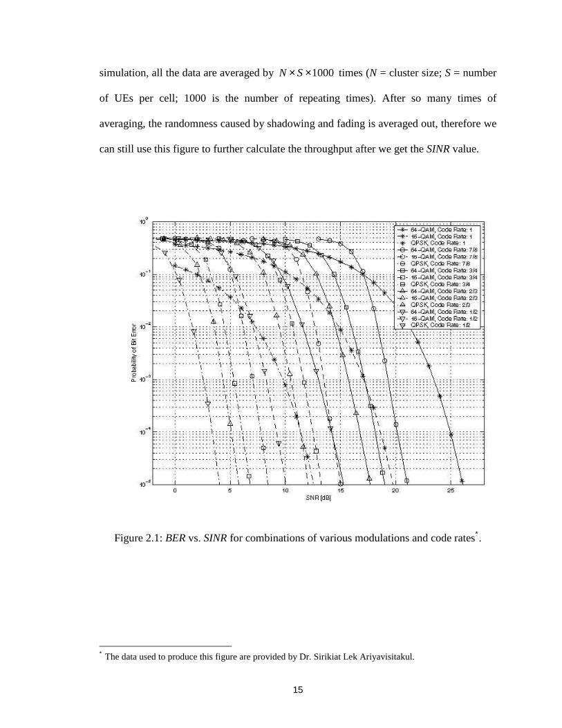
15

simulation, all the data are averaged by 1000×× SN times (N = cluster size; S = number

of UEs per cell; 1000 is the number of repeating times). After so many times of

averaging, the randomness caused by shadowing and fading is averaged out, therefore we

can still use this figure to further calculate the throughput after we get the SINR value.

Figure 2.1: BER vs. SINR for combinations of various modulations and code rates∗.

∗ The data used to produce this figure are provided by Dr. Sirikiat Lek Ariyavisitakul.

16

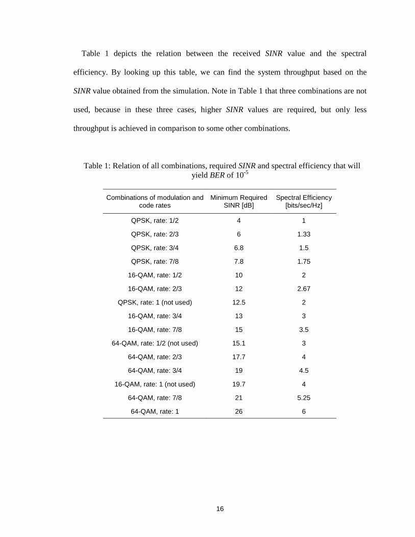
Table 1 depicts the relation between the received SINR value and the spectral

efficiency. By looking up this table, we can find the system throughput based on the

SINR value obtained from the simulation. Note in Table 1 that three combinations are not

used, because in these three cases, higher SINR values are required, but only less

throughput is achieved in comparison to some other combinations.

Table 1: Relation of all combinations, required SINR and spectral efficiency that willyield BER of 10-5

Combinations of modulation andcode rates

Minimum RequiredSINR [dB]

Spectral Efficiency[bits/sec/Hz]

QPSK, rate: 1/2 4 1

QPSK, rate: 2/3 6 1.33

QPSK, rate: 3/4 6.8 1.5

QPSK, rate: 7/8 7.8 1.75

16-QAM, rate: 1/2 10 2

16-QAM, rate: 2/3 12 2.67

QPSK, rate: 1 (not used) 12.5 2

16-QAM, rate: 3/4 13 3

16-QAM, rate: 7/8 15 3.5

64-QAM, rate: 1/2 (not used) 15.1 3

64-QAM, rate: 2/3 17.7 4

64-QAM, rate: 3/4 19 4.5

16-QAM, rate: 1 (not used) 19.7 4

64-QAM, rate: 7/8 21 5.25

64-QAM, rate: 1 26 6

17

2.3 Cellular Layout

Two different values for the cluster size (N) are considered: N = 4 and N = 1 cases.

Sections 2.3-2.5 describes the N = 4 case and Section 2.7 discusses the N = 1 case. Cells

with different sizes are investigated. The cell radii are 2000 m, 1000 m, and 500 m, for

large, medium, and small cells, respectively.

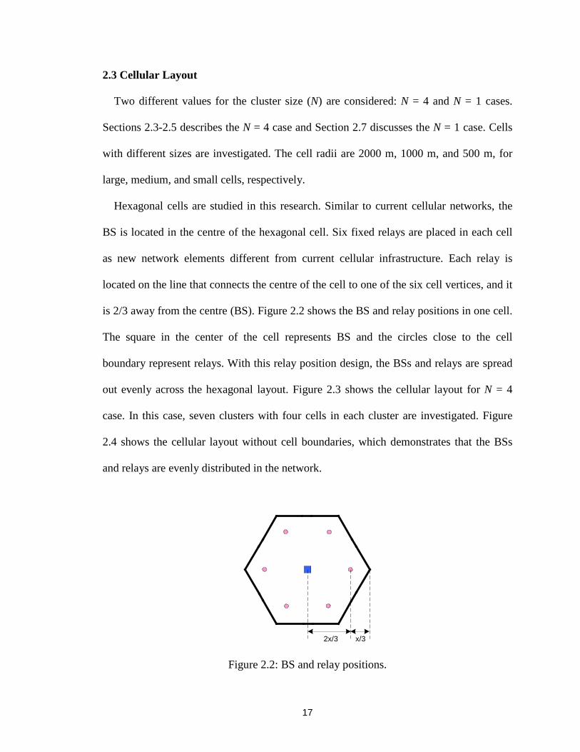
Hexagonal cells are studied in this research. Similar to current cellular networks, the

BS is located in the centre of the hexagonal cell. Six fixed relays are placed in each cell

as new network elements different from current cellular infrastructure. Each relay is

located on the line that connects the centre of the cell to one of the six cell vertices, and it

is 2/3 away from the centre (BS). Figure 2.2 shows the BS and relay positions in one cell.

The square in the center of the cell represents BS and the circles close to the cell

boundary represent relays. With this relay position design, the BSs and relays are spread

out evenly across the hexagonal layout. Figure 2.3 shows the cellular layout for N = 4

case. In this case, seven clusters with four cells in each cluster are investigated. Figure

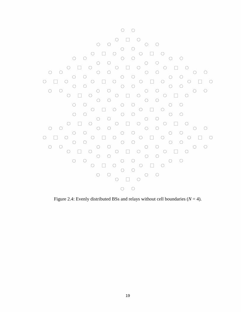
2.4 shows the cellular layout without cell boundaries, which demonstrates that the BSs

and relays are evenly distributed in the network.

2x/3 x/3

Figure 2.2: BS and relay positions.

18

Figure 2.3: Cellular layout (N = 4).

19

Figure 2.4: Evenly distributed BSs and relays without cell boundaries (N = 4).

20

2.4 Relaying Channel Partition Scheme

The terminology “ channel” may have different meanings in different wireless systems.

In this research we consider a non-CDMA system, which can be a TDMA or an OFDM

type. In a TDMA system, “ channel” is a time slot, while in an OFDM system, “ channel”

corresponds to frequency and/or time slot.

In a relaying network, an extra channel, relaying channel (between relay and UE), is

needed by a relay to forward the signal to a UE [4,29]. In analog relaying, this relaying

channel can be the same channel between the BS and relay, called by some researchers as

“ on-channel relaying” [10]. Due to the mechanism of on-channel relaying, the feedback

from the transmitter to the receiver of a relay is expected. This feedback problem must be

dealt with before the on-channel relaying technology can be implemented.

In the meanwhile, we may turn to other sources for relaying channels. The unlicensed

band is one of the appealing considerations due to the reasons that 1) unlicensed bands

are much more inexpensive than licensed bands and 2) any error occurred in the course of

relaying will only affect those UEs who need relaying, not the rest who receive signals

directly from the BS and use the licensed band. The side effect of utilizing unlicensed

bands is that it will complicate the structure and function of the UE and relay, since they

need to operate in the dual-band mode (licensed bands and unlicensed bands). [16] is a

detailed study of using the unlicensed bands for relaying in cellular CDMA networks.

Also, some channels can be exclusively reserved for relaying purpose. However since

the spectrum is a limited resource, this channel reservation approach is not desirable.

Instead of reserving, searching for any vacant channels for relaying might also be an

idea. However obviously this approach limits the opportunities for UEs to obtain relaying

21

assistance, since only when there are vacant channels available in the network can

relaying be implemented.

In this research we have the following pessimistic assumptions: 1) The investigated

cellular mobile network is fully loaded and no channels are to be reserved for relaying

purposes. 2) In each cell the number of channels equals the number of UEs. Therefore, all

relaying channels must be obtained via further reusing channels from the system. This is

an aggressive strategy, but it will be the most desired one if it works well, because no

extra radio resources are consumed while improving poor radio links. However, as can be

imagined, the assumptions made above will cause denser channel reuse and will result in

increased co-channel interference. In an effort to minimize these shortcomings and seek a

suitable approach for relaying channel acquisition, we have found a relaying channel

partition scheme with only controlled co-channel interference and least computational

overhead and it is detailed below. Note that only the downlink scenario is considered in

this relaying channel partition scheme.

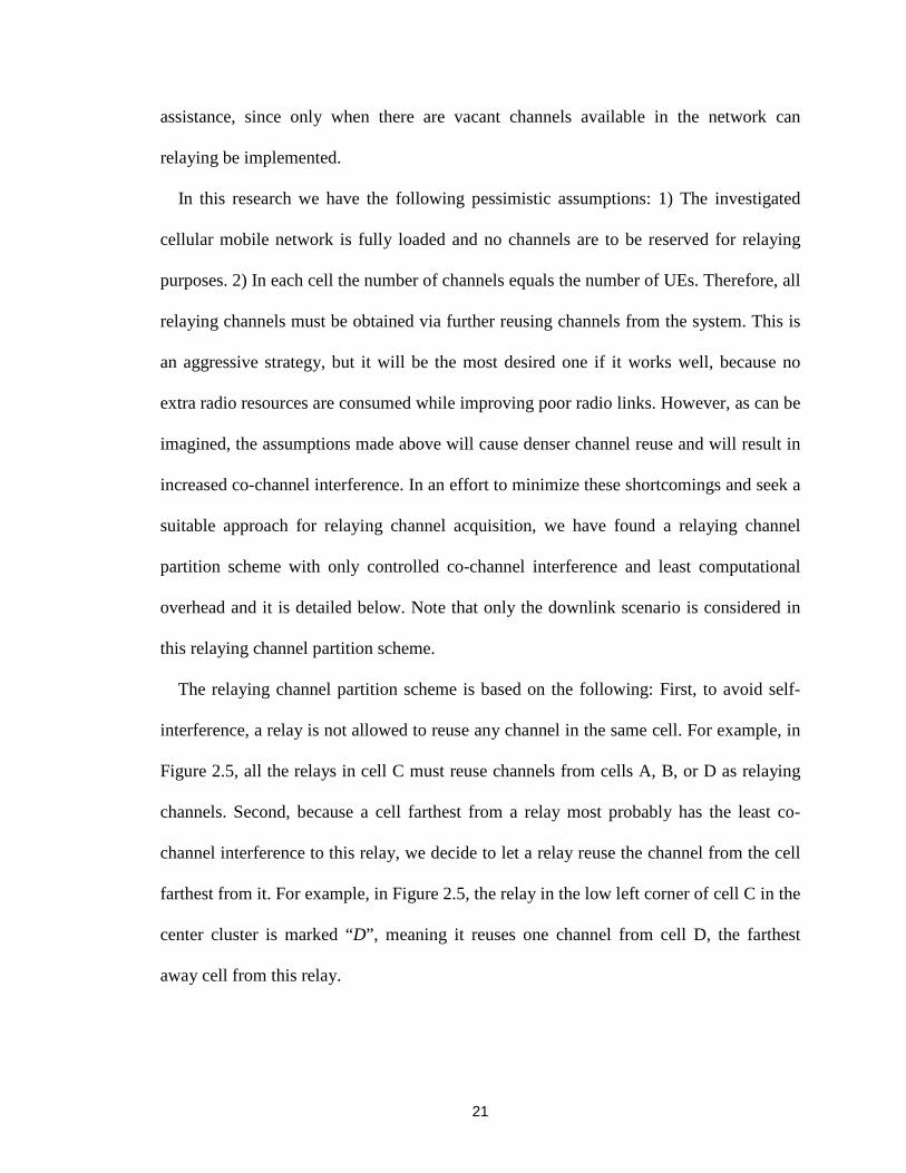
The relaying channel partition scheme is based on the following: First, to avoid self-

interference, a relay is not allowed to reuse any channel in the same cell. For example, in

Figure 2.5, all the relays in cell C must reuse channels from cells A, B, or D as relaying

channels. Second, because a cell farthest from a relay most probably has the least co-

channel interference to this relay, we decide to let a relay reuse the channel from the cell

farthest from it. For example, in Figure 2.5, the relay in the low left corner of cell C in the

center cluster is marked “ D” , meaning it reuses one channel from cell D, the farthest

away cell from this relay.

22

C

A

B

D

C

A

B

D

A

B

D

C

A

B

D

C

A

B

D

C

A

B

D

C

A

B

D

C

D

Figure 2.5: One relay reusing a channel from cell D.

23

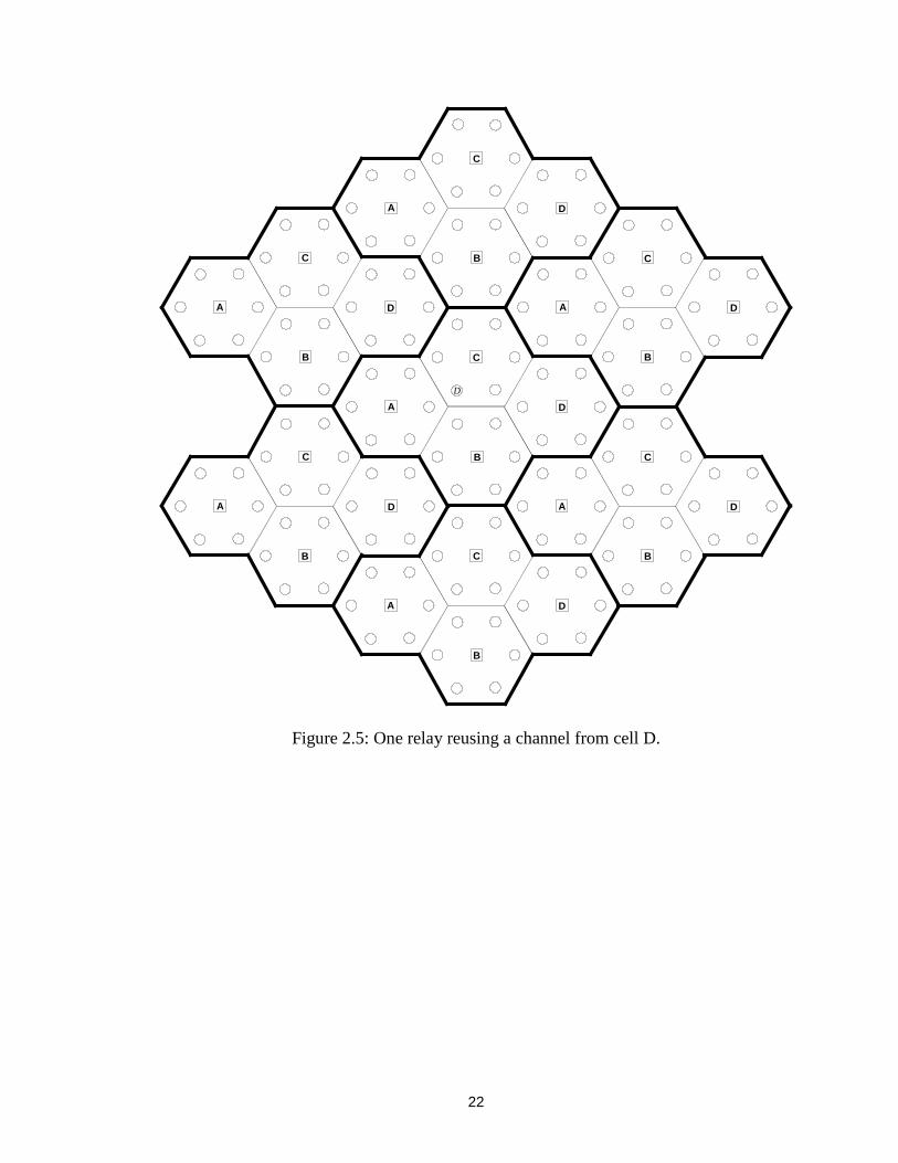
In Figure 2.6, all the relays reusing channels from cell D are marked out. It can be seen

that in each cluster, six relays will reuse channels from cell D as relaying channels. In

order to avoid these six relays reusing the same channel, all channels belonging to cell D

are divided into six disjoint groups with equal numbers of channels, and each relay reuses

one group of them. For example, if there are 48 channels per cell, each relay will be

assigned 8 channels. In Figure 2.6, a relay marked “ D3” means it reuses the third group of

channels from cell D.

C

A

B

D

C

A

B

D

A

B

D

C

A

B

D

C

A

B

D

C

A

B

D

C

A

B

D

1D2D

4D

3D

5D

6D

2D

4D

3D

5D

6D

1D2D

4D

3D

5D

6D

1D2D

4D

3D

5D

6D

1D2D

5D

6D

5D

6D

5D

6D

4D

3D

4D

3D

4D

3D

1D2D

1D2D

C

1D

Figure 2.6: All relays reusing channels from cell D.

24

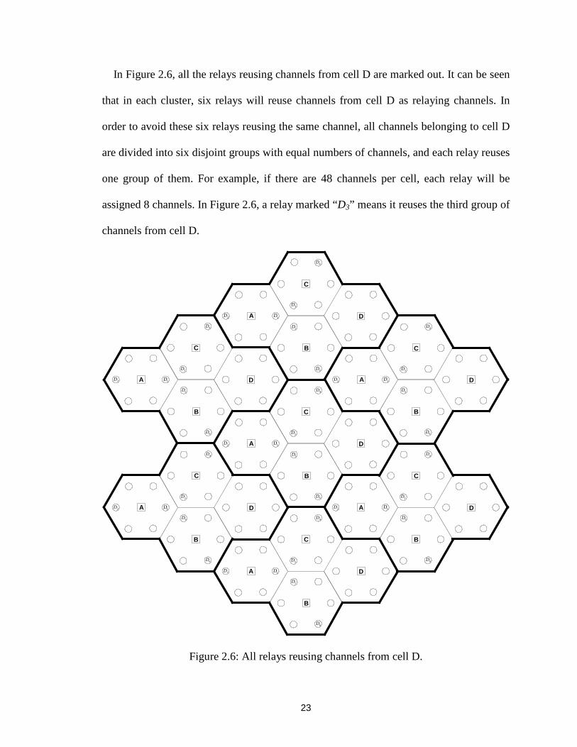
Figure 2.7 shows the overall channel partition scheme with the aforementioned

channel-reusing criterion applied to all relays. Note that in this relaying channel partition

scheme, no two relays in a cluster will choose the same relaying channel based on our

design.

Figure 2.7: Cell layout and relaying channel partition scheme.

C

A

B

D

C

A

B

D

A

B

D

C

A

B

D

C

A

B

D

C

A

B

D

C

A

B

D

1C

1C

1C

2B

1D2D

1B 2C

1A

4D

3B4B

3D

2A

5D 5A

3C4C

6A 6D

5B 6C

3A 4A

5C 6B

1C

2B

2D

1B 2C

1A

4D

3B4B

3D

2A

5D 5A

3C4C

6A 6D

5B 6C

3A 4A

5C 6B

2B

1D2D

1B 2C

1A

4D

3B4B

3D

2A

5D 5A

3C

6A 6D

5B 6C

3A 4A

5C 6B

1C 2B

1D2D

1B 2C

1A

4D

3B4B

3D

2A

5D 5A

3C4C

6A 6D

5B 6C

3A 4A

5C 6B

5B 6C

3A 4A

5C 6B

5B 6C

3A 4A

5C 6B

5B 6C

3A 4A

5C 6B

2B

1D2D

1B 2C

5D 5A

3C4C

6A 6D

5D 5A

3C4C

6A 6D

5D 5A

3C4C

6A 6D

1A

4D

3B4B

3D

2A

1A

4D

3B4B

3D

2A

1A

4D

3B4B

3D

2A

1C 2B

1D2D

1B 2C

1C 2B

1D2D

1B 2C

C

1D

4C

25

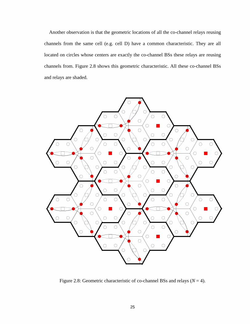
Another observation is that the geometric locations of all the co-channel relays reusing

channels from the same cell (e.g. cell D) have a common characteristic. They are all

located on circles whose centers are exactly the co-channel BSs these relays are reusing

channels from. Figure 2.8 shows this geometric characteristic. All these co-channel BSs

and relays are shaded.

Figure 2.8: Geometric characteristic of co-channel BSs and relays (N = 4).

26

The aforementioned fixed relaying channel selection scheme not only applies to the

cluster size N = 4 case, but works well for any cluster size. N = 1 case is a special one and

it is discussed in Section 3.3. The same geometric characteristic exists for all N values as

well. Appendix A shows the above described geometric characteristic for N = 3 and N = 7

cases.

The fixed relay position makes this relaying channel partition scheme a reality. The

main advantage of this scheme is the fact that it is a “ preset” way of channel partition;

there are no need for the complicated channel selection schemes and complicated channel

measuring schemes, and there is no overhead calculation. Whenever a relay requires a

relaying channel, it simply uses a channel from a set of channels allocated to it.

This relaying channel partition scheme is “ sub-optimum” due to the fact that this is a

fixed channel assignment, not a dynamic channel assignment based on the instantaneous

state of all the channels. In other words, only the distances between the BSs and relays

are considered when relaying channel partition scheme is defined. Shadowing and multi-

path fading are not taken into account. However, a significant amount of signalling

overhead will be inevitable if applying a dynamic channel selection, which might not be

feasible for a large cellular system.

Sometimes a UE requiring relaying finds an appropriate relay, but all the channels the

relay has are used at the moment. In this case, the relay denies the relaying service for

this UE. Then the UE has to go through a “ sub-optimal route” ; i.e., the UE turns to the

next relay or BS whichever is the second best, based on the relay selection schemes

explained in Section 2.5 (See (3) and (4)). We refer to this situation as “ Optimal-Route-

Blockage (ORB)” .

27

2.5 Relay Selection∗∗∗∗

Number of relays and how they are placed in a cell are specified in Section 2.3. A UE

then has two choices to receive signals: either from the BS or from one of the six relays.

This section describes the three algorithms used to determine from which node (BS or

relays) a UE will receive its signal. The algorithms are based on the following three

criteria: distance, pathloss and SINR. These three criteria have their own advantages and

disadvantages, for instance, the distance-based algorithm is the simplest to implement

with the assistance of GPS (Global Positioning System) technology [12,13], but the

performance enhancement it introduces is the least among the three algorithms. The

SINR-based algorithm produces the greatest performance improvement; conversely, it

involves more signalling overhead.

In all the three relay selection algorithms, we assume all six fixed relays are placed in

strategic locations with good receiving signals from the BS. The AMC mode will be

decided based on the SINR level between the relay and UE. The BS-relay link is assumed

to be good enough to support this mode of operation. In other words, the links between

the BS and the relays are assumed to be good enough to support the highest AMC mode

with negligible errors, though it will actually use the level that relay-UE link is using.

This assumption is not an unrealistic one, but made in order to simplify the system

model. In fact, it can be easily accomplished by placing the relays at high place above

any obstructions to ensure that there exists a Line of Sight path between the relays and

the BS. Also directional antennas and MIMO antennas can be used to guarantee a strong

signal between the BS and the relays.

∗ A UE can actually use the relay selection algorithms to select either a BS or a relay.

28

2.5.1 Distance-based Algorithm

This algorithm is solely based on the distances between the UE and BS and six relays.

Let us find the boundary (locus) on which the receiving signal Pr1 from the BS and the

receiving signal Pr2 from the relay are identical when shadowing and multipath fading are

averaged out. Since

Pr1 4

1d

kPBS= , Pr2 4

2d

kPrel= ,

where k is a constant, setting Pr1 = Pr2 yields

42

41 d

P

d

P relBS = .

In the above PBS is the BS transmit power, Prel is the relay transmit power, d1 is the

distance between the BS and the UE, and d2 is the distance between the relay and the UE.

Since PBS and Prel are usually constants,

==rel

BS

P

P

d

d4

2

41 constant ;

therefore, d1 / d2 is a constant as well. It can be shown that if the ratio of the distances of

a moving point to two fixed points is a constant, the locus meeting this requirement is a

circle. For the proof of this, refer to Appendix B. This circle is exactly the boundary that

we are trying to figure out. By applying different values to PBS and Prel, we can get the

location of the centre of the circle and its radius.

Figure 2.9 shows the coverage boundary of the BS and six relays in a hexagonal cell

with PBS = 10 W and Prel = 1 W.

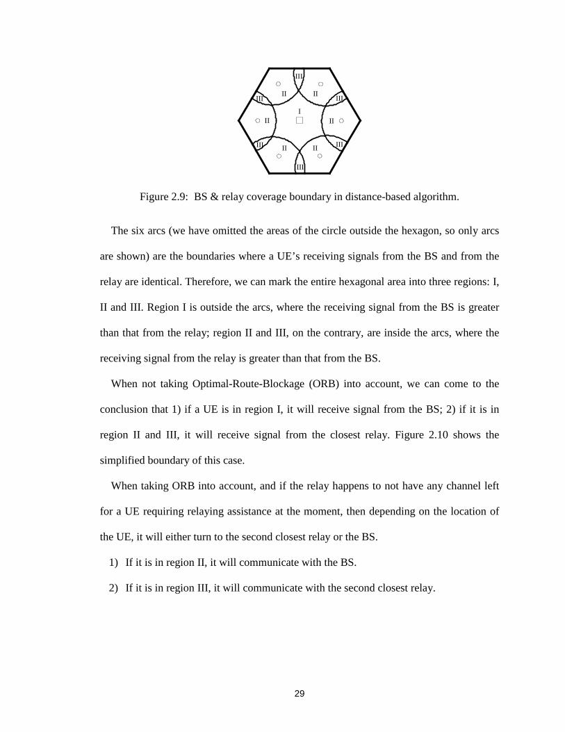
29

I

II

III

II

II II

II II

III

III

III

III

III

Figure 2.9: BS & relay coverage boundary in distance-based algorithm.

The six arcs (we have omitted the areas of the circle outside the hexagon, so only arcs

are shown) are the boundaries where a UE’s receiving signals from the BS and from the

relay are identical. Therefore, we can mark the entire hexagonal area into three regions: I,

II and III. Region I is outside the arcs, where the receiving signal from the BS is greater

than that from the relay; region II and III, on the contrary, are inside the arcs, where the

receiving signal from the relay is greater than that from the BS.

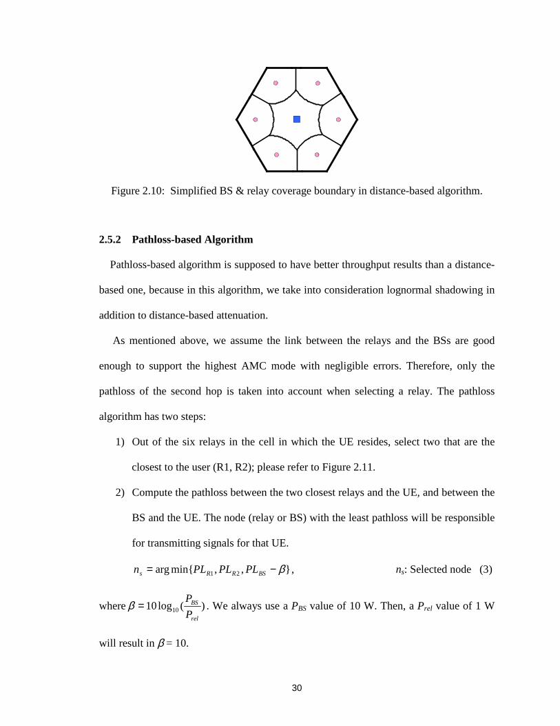
When not taking Optimal-Route-Blockage (ORB) into account, we can come to the

conclusion that 1) if a UE is in region I, it will receive signal from the BS; 2) if it is in

region II and III, it will receive signal from the closest relay. Figure 2.10 shows the

simplified boundary of this case.

When taking ORB into account, and if the relay happens to not have any channel left

for a UE requiring relaying assistance at the moment, then depending on the location of

the UE, it will either turn to the second closest relay or the BS.

1) If it is in region II, it will communicate with the BS.

2) If it is in region III, it will communicate with the second closest relay.

30

Figure 2.10: Simplified BS & relay coverage boundary in distance-based algorithm.

2.5.2 Pathloss-based Algorithm

Pathloss-based algorithm is supposed to have better throughput results than a distance-

based one, because in this algorithm, we take into consideration lognormal shadowing in

addition to distance-based attenuation.

As mentioned above, we assume the link between the relays and the BSs are good

enough to support the highest AMC mode with negligible errors. Therefore, only the

pathloss of the second hop is taken into account when selecting a relay. The pathloss

algorithm has two steps:

1) Out of the six relays in the cell in which the UE resides, select two that are the

closest to the user (R1, R2); please refer to Figure 2.11.

2) Compute the pathloss between the two closest relays and the UE, and between the

BS and the UE. The node (relay or BS) with the least pathloss will be responsible

for transmitting signals for that UE.

},,min{arg 21 β−= BSRRs PLPLPLn , ns: Selected node (3)

where )(log10 10rel

BS

P

P=β . We always use a PBS value of 10 W. Then, a Prel value of 1 W

will result in β = 10.

31

2.5.3 SINR-based Algorithm

This algorithm is expected to yield an enhanced performance in comparison to the

other two algorithms (distance and pathloss). Similar to the pathloss-based type, SINR-

based algorithm has two steps:

1) Out of the six relays in the cell in which the UE resides, select two that are the

closest to the UE (R1, R2); please refer to Figure 2.11.

2) Compute the SINR between the two closest relays and the UE, and between the

BS and the UE. The node (relay or BS) with the maximum SINR will be

responsible for transmitting signals for the UE.

},,max{arg 21 BSRRs SINRSINRSINRn = , ns: Selected node (4)

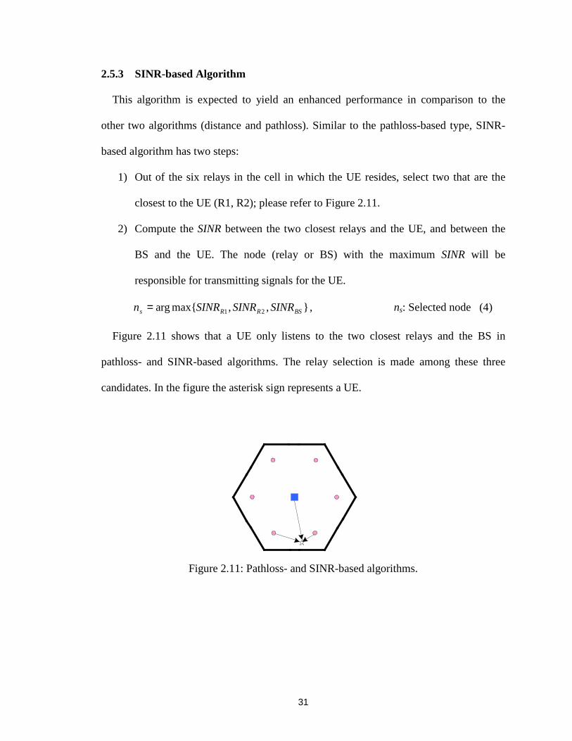
Figure 2.11 shows that a UE only listens to the two closest relays and the BS in

pathloss- and SINR-based algorithms. The relay selection is made among these three

candidates. In the figure the asterisk sign represents a UE.

Figure 2.11: Pathloss- and SINR-based algorithms.

32

2.6 Diversity

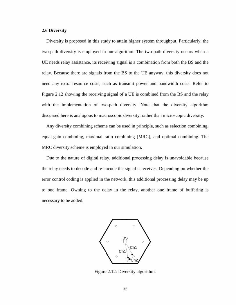
Diversity is proposed in this study to attain higher system throughput. Particularly, the

two-path diversity is employed in our algorithm. The two-path diversity occurs when a

UE needs relay assistance, its receiving signal is a combination from both the BS and the

relay. Because there are signals from the BS to the UE anyway, this diversity does not

need any extra resource costs, such as transmit power and bandwidth costs. Refer to

Figure 2.12 showing the receiving signal of a UE is combined from the BS and the relay

with the implementation of two-path diversity. Note that the diversity algorithm

discussed here is analogous to macroscopic diversity, rather than microscopic diversity.

Any diversity combining scheme can be used in principle, such as selection combining,

equal-gain combining, maximal ratio combining (MRC), and optimal combining. The

MRC diversity scheme is employed in our simulation.

Due to the nature of digital relay, additional processing delay is unavoidable because

the relay needs to decode and re-encode the signal it receives. Depending on whether the

error control coding is applied in the network, this additional processing delay may be up

to one frame. Owning to the delay in the relay, another one frame of buffering is

necessary to be added.

BS

Ch1Ch1

Ch2

Figure 2.12: Diversity algorithm.

33

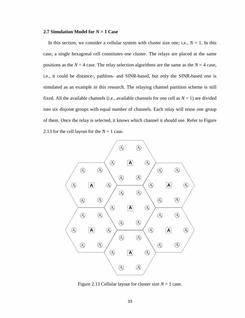
2.7 Simulation Model for N = 1 Case

In this section, we consider a cellular system with cluster size one; i.e., N = 1. In this

case, a single hexagonal cell constitutes one cluster. The relays are placed at the same

positions as the N = 4 case. The relay selection algorithms are the same as the N = 4 case,

i.e., it could be distance-, pathloss- and SINR-based, but only the SINR-based one is

simulated as an example in this research. The relaying channel partition scheme is still

fixed. All the available channels (i.e., available channels for one cell as N = 1) are divided

into six disjoint groups with equal number of channels. Each relay will reuse one group

of them. Once the relay is selected, it knows which channel it should use. Refer to Figure

2.13 for the cell layout for the N = 1 case.

A

A

A

A

A

A

A3A

4A 5A

6A

1A2A

3A

4A 5A

6A

1A2A

3A

4A 5A

6A

1A2A

3A

4A 5A

6A

1A2A

3A

4A 5A

6A

1A2A

3A

4A 5A

6A

1A2A

3A

4A 5A

6A

1A2A

Figure 2.13 Cellular layout for cluster size N = 1 case.

34

Chapter 3 Simulation Algorithm

This chapter primarily concerns the simulation algorithms. First, the environmental

parameters used in the simulation are specified. Then, the simulation algorithm is

described.

3.1 Environment and Parameters Assumptions

Below is a list of parameters used in the simulation algorithms. They are typical data

widely used in simulating cellular networks. They were approved by the research

sponsor, Nortel Networks, prior to be used in the simulation.

• Pathloss propagation exponent: n = 4

• Lognormal shadowing with a standard deviation: σ = 8 dB

• Flat Rayleigh fading

• Slow fading: since we aim at achieving high data rate coverage. Fast fading only

happens for very low data rate applications [9].

• Doppler effects are ignored: since the effects due to Doppler spread are negligible for

slow fading channels [9].

• Simulation area: hexagonal cells with the cell radius R = 2000 m, 1000 m or 500 m,

4-cell and 1-cell clusters. Seven clusters are investigated, i.e., the first tier co-channel

interference is considered in our simulation.

• RF carrier = 2 GHz

• Transmission bandwidth: W = 5 MHz

• Thermal noise with a noise figure: F = 8 dB

35

• Isotropic antennas (with unit gain) for the BS, fixed relay and UE

• No power control: when adaptive modulation and coding scheme is used, power

control does not contribute much towards the throughput increase [6].

• Base station transmit power: PBS = 10 W

• Fixed relay transmit power: Prel = 0.1 W, 0.3 W, 1 W

• Downlink scenario only: since the requested data rate from this direction is likely to

be higher than the uplink case.

Note that the channel model elaborated above as well as the omni-directional antenna

assumption is valid for the BS-to-UE and relay-to-UE links. As mentioned in Section 2.2,

the BS-to-relay link is assumed to be effective enough to support the highest AMC mode

with negligible errors.

3.2 Simulation Algorithm for N = 4 Case

In this simulation, we compare the system performances of the with-relaying and

without-relaying cases.

The UEs are placed randomly across the cluster (4 cells / cluster or 1 cell / cluster)

with S UEs per cell. We have chosen six values for S: S = 12, 24, 36, 48, 60 or 72.

For the without-relaying case, all UEs will receive signals from the BS. Let PS denote

the received signal power.

The formula to calculate the interference power is as follows:

PI = P1 + P2 + … + P6 ,

where P1, … , P6 are the interference powers from the co-channel BSs.

The noise power is calculated according to the following formula:

36

PN = Kb × T × W × F = 1.306 × 10-13 watts,

where Kb is the Boltzmann’s constant (1.38 × 10-23 Joules/Kelvin), T is the system

temperature (300 K), W is the transmission bandwidth (5 MHz), and F is the noise figure

(6.31 = 8dB).

Now SINR can be calculated as:

IN

S

PP

PSINR

+= . (3.1)

For the with-relaying case, as described before, six relays are placed in each cell. First

a node (BS or relay) is selected according to the relay selection schemes described in

Chapter 2, i.e. distance-, pathloss- or SINR-based algorithms. The received signal can be

either from the BS or from the relay depending on which node the UE is communicating

with. The interference power is different from the without-relaying case, because we need

to consider the interference from other relays using the same channel in addition to the

interference generated by co-channel BSs.

The formula below shows how to calculate the total interference power:

PI = P1 + P2 + … + P13 ,

where if the received signal is from the BS, P1, … , P6 are the interference powers from

the co-channel BSs and P7, … , P13 are the interference powers from the relays using the

same channel. If the received signal is from the relay, P1, … , P7 are the interference

powers from the co-channel BSs and P8, … , P13 are the interference powers from the

relays using the same channel. Here the worst case scenario in calculating the

interference is considered; in other words, we assume all the relays are using all channels

allocated to them to transmit signals, though in fact sometimes some channels will not be

used.

37

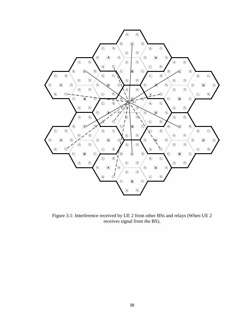
Figures 3.1 and 3.2 show the interference sources for the above two cases,

respectively. UE 2 and UE 6 are two randomly selected UE positions. In the case of no

relays, both of these two UEs receive signals from the BS. After all the relays are in

place, due to their different locations, UE 2 still communicates with the BS, while UE 6

chooses a relay. So the interference sources for these two UEs are different, hence the

ways to calculate the interference are different. They are depicted in the above paragraph

and shown in these two figures. In the figures, solid lines indicate the interference

received by a UE from the co-channel BSs, while dotted lines indicate the interference

received by a UE from the relays in other clusters using the same channel. The asterisk

sign in the figures represents a UE.

Once the interference sources are determined for a UE, SINR can be recalculated using

(3.1).

After obtaining the SINR for both without-relay and with-relay cases for each UE,

Table 1 is used to find out the throughput (spectral efficiency) for that UE. Then, the

throughput values of all the UEs in the innermost cluster are summed up and

subsequently divided with the total numbers of UEs in one cluster, which is equal to the

number of UEs per cell (S) times the cluster size (N). The above steps are repeated for a

total of 1000 times to calculate the sum and average throughput.

Please refer to Figures 3.3 and 3.4 for the flowcharts of distance-, pathloss- and SINR-

based algorithms. Figure 3.3 shows the case when ORB (explained in Chapter 2) is not

taken into account; Figure 3.4 shows the case when ORB is taken into account.

38

C

A

B

D

C

A

B

D

A

B

D

C

A

B

D

C

A

B

D

C

A

B

D

C

A

B

D

1C

1C

1C

2B

1D2D

1B 2C

1A

4D

3B4B

3D

2A

5D 5A

3C4C

6A 6D

5B 6C

3A 4A

5C 6B

1C

2B

2D

1B 2C

1A

4D

3B4B

3D

2A

5D 5A

3C4C

6A 6D

5B 6C

3A 4A

5C 6B

2B

1D2D

1B 2C

1A

4D

3B4B

3D

2A

5D 5A

3C

6A 6D

5B 6C

3A 4A

5C 6B

1C 2B

1D2D

1B 2C

1A

4D

3B4B

3D

2A

5D 5A

3C4C

6A 6D

5B 6C

3A 4A

5C 6B

5B 6C

3A 4A

5C 6B

5B 6C

3A 4A

5C 6B

5B 6C

3A 4A

5C 6B

2B

1D2D

1B 2C

5D 5A

3C4C

6A 6D

5D 5A

3C4C

6A 6D

5D 5A

3C4C

6A 6D

1A

4D

3B4B

3D

2A

1A

4D

3B4B

3D

2A

1A

4D

3B4B

3D

2A

1C 2B

1D2D

1B 2C

1C 2B

1D2D

1B 2C

C

1D

4C

UE2

Figure 3.1: Interference received by UE 2 from other BSs and relays (When UE 2receives signal from the BS).

39

C

A

B

D

C

A

B

D

A

B

D

C

A

B

D

C

A

B

D

C

A

B

D

C

A

B

D

1C

1C

1C

2B

1D2D

1B 2C

1A

4D

3B4B

3D

2A

5D 5A

3C4C

6A 6D

5B 6C

3A 4A

5C 6B

1C

2B

2D

1B 2C

1A

4D

3B4B

3D

2A

5D 5A

3C4C

6A 6D

5B 6C

3A 4A

5C 6B

2B

1D2D

1B 2C

1A

4D

3B4B

3D

2A

5D 5A

3C

6A 6D

5B 6C

3A 4A

5C 6B

1C 2B

1D2D

1B 2C

1A

4D

3B4B

3D

2A

5D 5A

3C4C

6A 6D

5B 6C

3A 4A

5C 6B

5B 6C

3A 4A

5C 6B

5B 6C

3A 4A

5C 6B

5B 6C

3A 4A

5C 6B

2B

1D2D

1B 2C

5D 5A

3C4C

6A 6D

5D 5A

3C4C

6A 6D

5D 5A

3C4C

6A 6D

1A

4D

3B4B

3D

2A

1A

4D

3B4B

3D

2A

1A

4D

3B4B

3D

2A

1C 2B

1D2D

1B 2C

1C 2B

1D2D

1B 2C

C

1D

4C

UE6

Figure 3.2: Interference received by UE 6 from other BSs and relays (When UE 6receives signal from a relay).

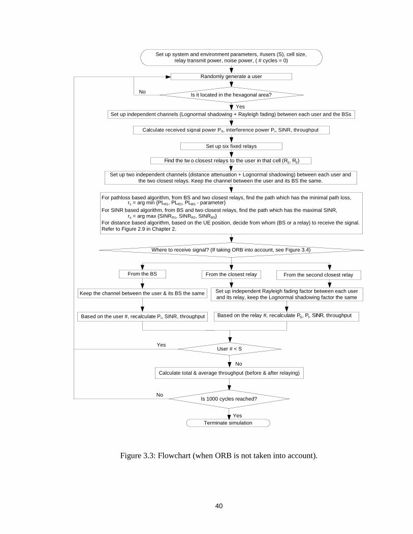
40

Set up system and environment parameters, #users (S), cell size,relay transmit power, noise power, ( # cycles = 0)

Randomly generate a user

Is it located in the hexagonal area?

Set up independent channels (Lognormal shadowing + Rayleigh fading) between each user and the BSs

Set up six fixed relays

Set up two independent channels (distance attenuation + Lognormal shadowing) between each user andthe two closest relays. Keep the channel between the user and its BS the same.

Yes

No

For pathloss based algorithm, from BS and two closest relays, find the path which has the minimal path loss,

For SINR based algorithm, from BS and two closest relays, find the path which has the maximal SINR,

For distance based algorithm, based on the UE position, decide from whom (BS or a relay) to receive the signal.Refer to Figure 2.9 in Chapter 2.

Calculate received signal power PS, interference power PI, SINR, throughput

Find the tw o closest relays to the user in that cell (R1, R2)

rs = arg min {PLR1, PLR2, PLBS - parameter}

rs = arg max {SINRR1, SINRR2, SINRBS}

Terminate simulation

Where to receive signal? (If taking ORB into account, see Figure 3.4)

From the BS From the closest relay From the second closest relay

Keep the channel between the user & its BS the same

User # < S

Set up independent Rayleigh fading factor between each userand its relay, keep the Lognormal shadowing factor the same

Calculate total & average throughput (before & after relaying)

Is 1000 cycles reached?No

Yes

Yes

No

Based on the user #, recalculate PI, SINR, throughput Based on the relay #, recalculate PS, PI, SINR, throughput

Figure 3.3: Flowchart (when ORB is not taken into account).

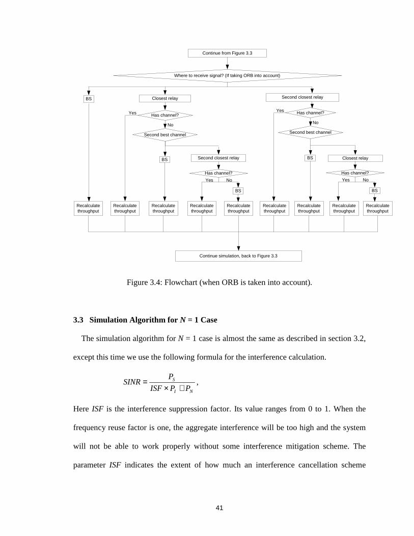
41

Where to receive signal? (If taking ORB into account)

BS Closest relay Second closest relay

Continue from Figure 3.3

Has channel? Has channel?Yes

No

Second best channel

BS

Recalculatethroughput

Recalculatethroughput

Recalculatethroughput

Recalculatethroughput

Recalculatethroughput

Recalculatethroughput

Recalculatethroughput

Recalculatethroughput

Recalculatethroughput

Second closest relay

Has channel?

Yes No

Yes

Second best channel

No

BS Closest relay

BS

Has channel?

Yes No

BS

Continue simulation, back to Figure 3.3

Figure 3.4: Flowchart (when ORB is taken into account).

3.3 Simulation Algorithm for N = 1 Case

The simulation algorithm for N = 1 case is almost the same as described in section 3.2,

except this time we use the following formula for the interference calculation.

NI

S

PPISF

PSINR

+×= ,

Here ISF is the interference suppression factor. Its value ranges from 0 to 1. When the

frequency reuse factor is one, the aggregate interference will be too high and the system

will not be able to work properly without some interference mitigation scheme. The

parameter ISF indicates the extent of how much an interference cancellation scheme

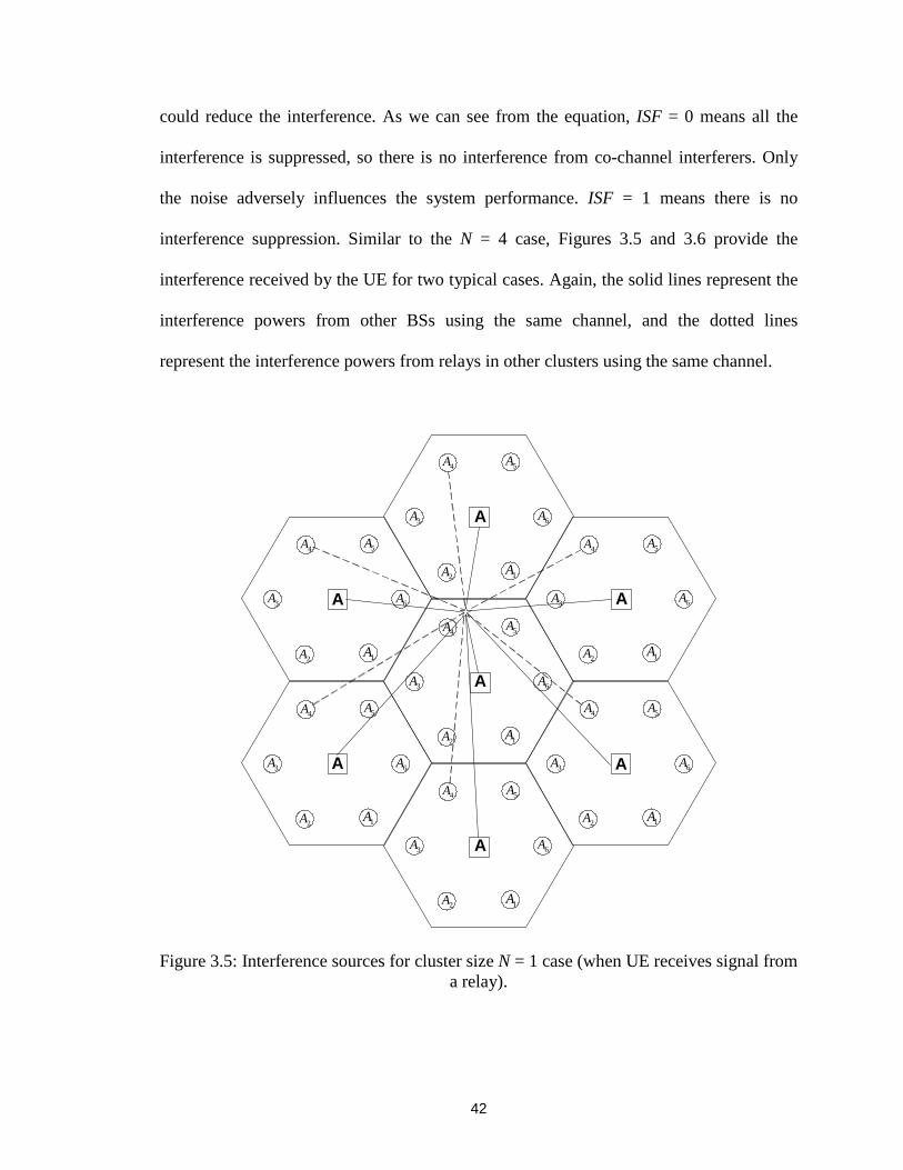
42

could reduce the interference. As we can see from the equation, ISF = 0 means all the

interference is suppressed, so there is no interference from co-channel interferers. Only

the noise adversely influences the system performance. ISF = 1 means there is no

interference suppression. Similar to the N = 4 case, Figures 3.5 and 3.6 provide the

interference received by the UE for two typical cases. Again, the solid lines represent the

interference powers from other BSs using the same channel, and the dotted lines

represent the interference powers from relays in other clusters using the same channel.

A

A

A

A

A

A

A3A

4A 5A

6A

1A2A

3A

4A 5A

6A

1A2A

3A

4A 5A

6A

1A2A

3A

4A 5A

6A

1A2A

3A

4A 5A

6A

1A2A

3A

4A 5A

6A

1A2A

3A

4A 5A

6A

1A2A

Figure 3.5: Interference sources for cluster size N = 1 case (when UE receives signal froma relay).

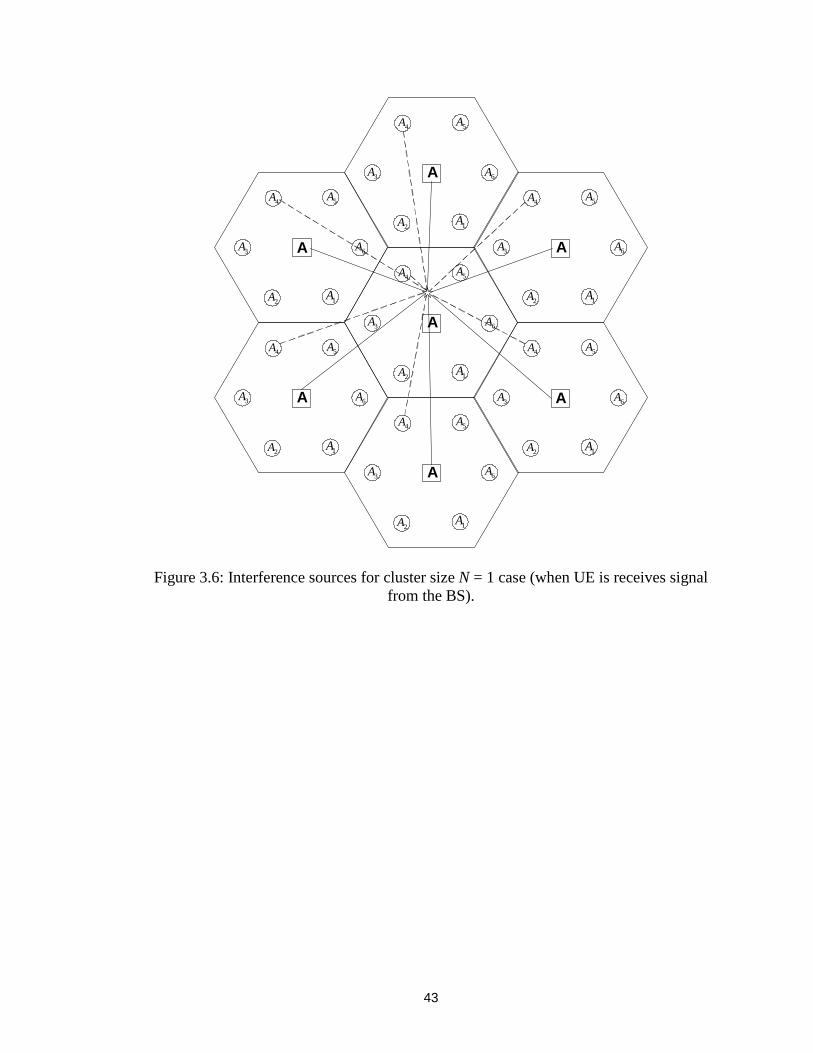
43

A

A

A

A

A

A

A

3A

4A 5A

6A

1A2A

3A

4A 5A

6A

1A2A

3A

4A 5A

6A

1A2A

3A

4A 5A

6A

1A2A

3A

4A 5A

6A

1A2A

3A

4A 5A

6A

1A2A

3A

4A 5A

6A

1A2A

Figure 3.6: Interference sources for cluster size N = 1 case (when UE is receives signalfrom the BS).

44

Chapter 4 Simulation Results, Part I: N = 4 Case

This chapter and the following one present the simulation results. This chapter is

focused on the results for the cluster size N = 4 case and the following chapter is focused

on N = 1 case.

The results shown in this and the following chapter are mainly based on SINR-based

algorithm, which yields the best output, though the average throughput improvement for

the three different relay selection algorithms demonstrated in Section 2.5 is given in

Section 4.4. This chapter also investigates the following points: the average throughput

improvement, the relay usage, the impact of ORB on system performance, the throughput

increase provided by diversity, the system sensitivity to the background noise, the

transmission bandwidth and the pathloss exponent. How often each combination of

modulation and coding is used is described in the latter portion of this chapter.

4.1 Average Spectral Efficiency of SINR-based Algorithm

Figures 4.1, 4.2 and 4.3 show the average throughput where cell radius is 2000 m,

1000 m and 500 m, respectively. From these three figures we can see that when using

relays in a cell, the throughput is greatly increased in all the three cases, comparing to

that of the no relaying case.

When the relay transmit power is increased, we get higher throughput. For example in

Figure 4.3 where R = 500 m, when user density is 72 and Prel = 0.1 W, the throughput

improvement is 0.7 bits/sec/Hz corresponding to a 22% increase (3.22 � 3.92). When we

increase Prel to 1 W, the throughput is increased by 42% (3.22 � 4.6).

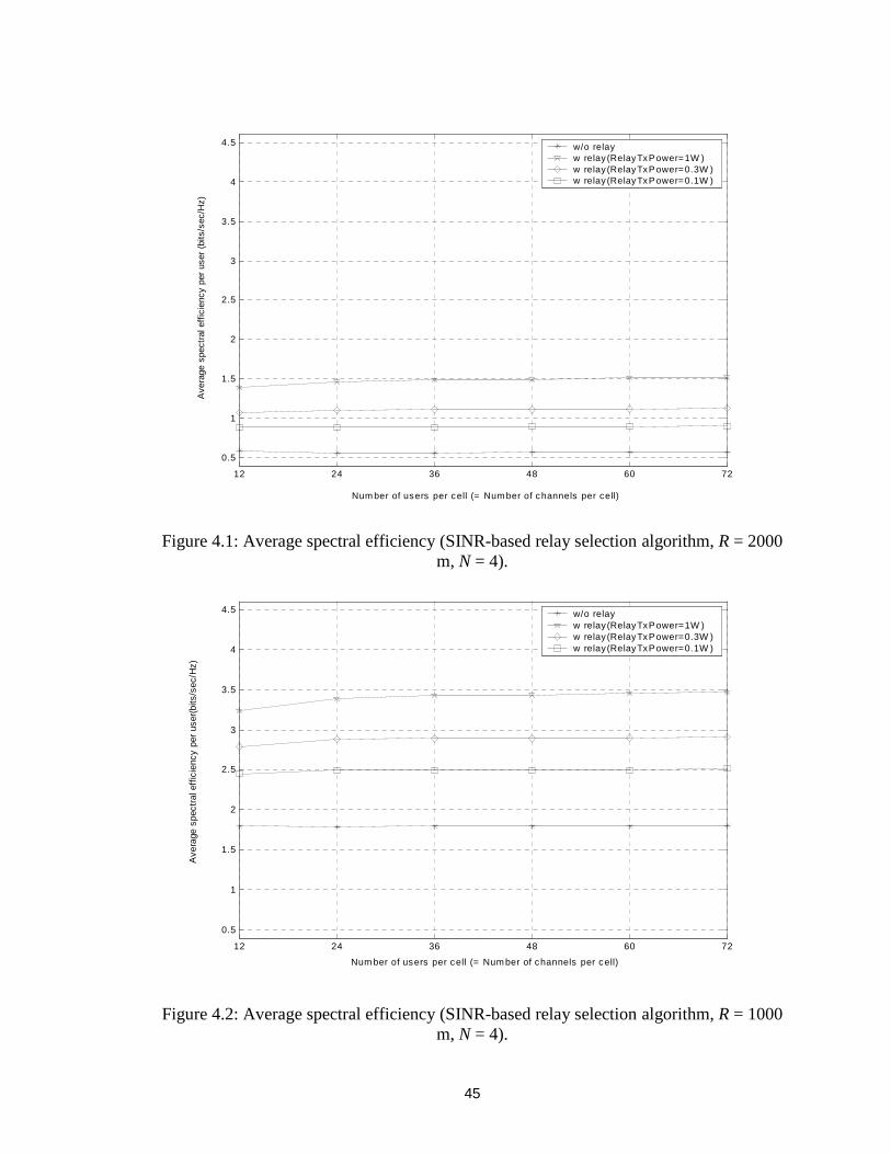
45

12 24 36 48 60 72

0.5

1

1.5

2

2.5

3

3.5

4

4.5

Num ber of users per cell (= Num ber of channels per cell)

Ave

rage

spe

ctra

l eff

icie

ncy

per

user

(bi

ts/s

ec/H

z)

w/o relayw relay (RelayTxPower=1W )w relay (RelayTxPower=0.3W )w relay (RelayTxPower=0.1W )

Figure 4.1: Average spectral efficiency (SINR-based relay selection algorithm, R = 2000m, N = 4).

12 24 36 48 60 72

0.5

1

1.5

2

2.5

3

3.5

4

4.5

Num ber of users per cell (= Num ber of channels per cell)

Ave

rage

spe

ctra

l eff

icie

ncy

per

user

(bits

/sec

/Hz)

w/o relayw relay(RelayTxPower=1W )w relay(RelayTxPower=0.3W )w relay(RelayTxPower=0.1W )

Figure 4.2: Average spectral efficiency (SINR-based relay selection algorithm, R = 1000m, N = 4).

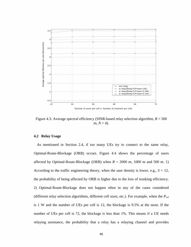
46

12 24 36 48 60 72

0.5

1

1.5

2

2.5

3

3.5

4

4.5

Number of users per cell (= Number of channels per cell)

Ave

rage

spe

ctra

l eff

icie

ncy

per

user

(bi

ts/s

ec/H

z)

w/o relayw relay(RelayTxPower=1W )w relay(RelayTxPower=0.3W )w relay(RelayTxPower=0.1W )

Figure 4.3: Average spectral efficiency (SINR-based relay selection algorithm, R = 500m, N = 4).

4.2 Relay Usage

As mentioned in Section 2.4, if too many UEs try to connect to the same relay,

Optimal-Route-Blockage (ORB) occurs. Figure 4.4 shows the percentage of users

affected by Optimal-Route-Blockage (ORB) when R = 2000 m, 1000 m and 500 m. 1)

According to the traffic engineering theory, when the user density is lower, e.g., S = 12,

the probability of being affected by ORB is higher due to the loss of trunking efficiency.

2) Optimal-Route-Blockage does not happen often in any of the cases considered

(different relay selection algorithms, different cell sizes, etc.). For example, when the Prel

is 1 W and the number of UEs per cell is 12, the blockage is 9.5% at the most. If the

number of UEs per cell is 72, the blockage is less than 1%. This means if a UE needs

relaying assistance, the probability that a relay has a relaying channel and provides

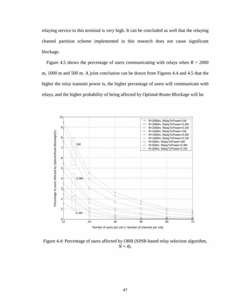
47

relaying service to this terminal is very high. It can be concluded as well that the relaying

channel partition scheme implemented in this research does not cause significant

blockage.

Figure 4.5 shows the percentage of users communicating with relays when R = 2000

m, 1000 m and 500 m. A joint conclusion can be drawn from Figures 4.4 and 4.5 that the

higher the relay transmit power is, the higher percentage of users will communicate with

relays, and the higher probability of being affected by Optimal-Route-Blockage will be.

12 24 36 48 60 720

1

2

3

4

5

6

7

8

9

10

Number of users per cell (= Number of channels per cell)

Per

cent

age

of u

sers

aff

ecte

d by

Opt

imal

-Rou

te-B

lock

age(

%)

R=2000m, RelayTxPower=1WR=2000m, RelayTxPower=0.3WR=2000m, RelayTxPower=0.1WR=1000m, RelayTxPower=1WR=1000m, RelayTxPower=0.3WR=1000m, RelayTxPower=0.1WR=500m, RelayTxPower=1WR=500m, RelayTxPower=0.3WR=500m, RelayTxPower=0.1W

1W

0.3W

0.1W

Figure 4.4: Percentage of users affected by ORB (SINR-based relay selection algorithm,N = 4).

48

12 24 36 48 60 7230

40

50

60

70

80

90

100

Number of users per cell (= Number of channels per cell)

Per

cent

age

of u

sers

com

mun

icat

ing

with

rel

ayer

s(%

)

R=2000m, RelayTxPower=1WR=2000m, RelayTxPower=0.3WR=2000m, RelayTxPower=0.1WR=1000m, RelayTxPower=1WR=1000m, RelayTxPower=0.3WR=1000m, RelayTxPower=0.1WR=500m, RelayTxPower=1WR=500m, RelayTxPower=0.3WR=500m, RelayTxPower=0.1W

1W

0.3W

0.1W

Figure 4.5: Percentage of users communicating with relays (SINR-based relay selectionalgorithm, N = 4).

4.3 Average Spectral Efficiency for with and without ORB Cases

Figures 4.6, 4.7 and 4.8 compare with and without Optimal-Route-Blockage (ORB)

cases when R = 500 m, 1000 m and 2000 m. For a “ without ORB” case, it is assumed that

a relay can always offer a relaying channel for a UE, whether the channel is actually

available or not. These three figures show that if ORB is not taken into account, the

throughput is slightly higher and does not fluctuate with the increase of number of users

per cell; if taking ORB into account, the performance slightly decreases, comparing to the

opposite case. We can come to a common conclusion from Figure 4.4 and these three

figures that the higher number of users per cell, the lower percentage of users being

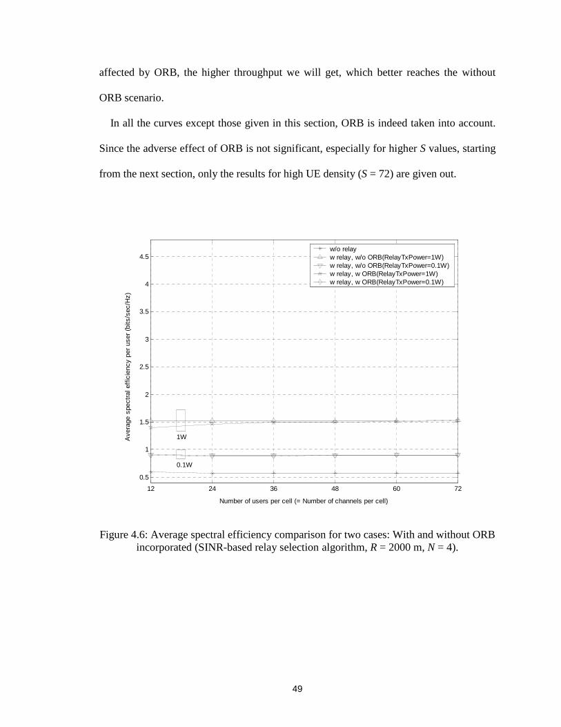
49

affected by ORB, the higher throughput we will get, which better reaches the without

ORB scenario.

In all the curves except those given in this section, ORB is indeed taken into account.

Since the adverse effect of ORB is not significant, especially for higher S values, starting

from the next section, only the results for high UE density (S = 72) are given out.

12 24 36 48 60 72

0.5

1

1.5

2

2.5

3

3.5

4

4.5

Number of users per cell (= Number of channels per cell)

Ave

rage

spe

ctra

l eff

icie

ncy

per

user

(bi

ts/s

ec/H

z)

w/o relayw relay, w/o ORB(RelayTxPower=1W)w relay, w/o ORB(RelayTxPower=0.1W)w relay, w ORB(RelayTxPower=1W)w relay, w ORB(RelayTxPower=0.1W)

1W

0.1W

Figure 4.6: Average spectral efficiency comparison for two cases: With and without ORBincorporated (SINR-based relay selection algorithm, R = 2000 m, N = 4).

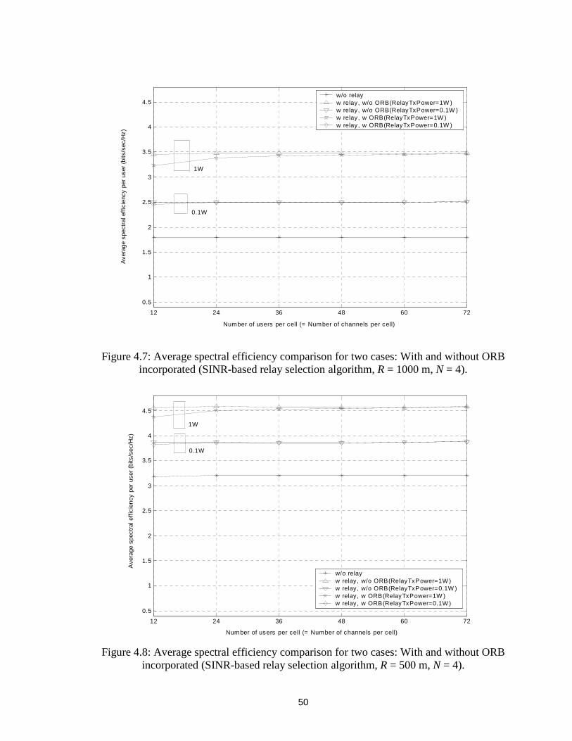
50

12 24 36 48 60 72

0.5

1

1.5

2

2.5

3

3.5

4

4.5

Number of users per cell (= Number of channels per cell)

Ave

rage

spe

ctra

l eff

icie

ncy

per

user

(bi

ts/s

ec/H

z)

w/o relayw relay, w/o ORB(RelayTxPower=1W )w relay, w/o ORB(RelayTxPower=0.1W )w relay, w ORB(RelayTxPower=1W )w relay, w ORB(RelayTxPower=0.1W )

1W

0.1W

Figure 4.7: Average spectral efficiency comparison for two cases: With and without ORBincorporated (SINR-based relay selection algorithm, R = 1000 m, N = 4).

12 24 36 48 60 72

0.5

1

1.5

2

2.5

3

3.5

4

4.5

Number of users per cell (= Number of channels per cell)

Ave

rage

spe

ctra

l eff

icie

ncy

per

user

(bi

ts/s

ec/H

z)

w/o relayw relay, w/o ORB(RelayTxPower=1W )w relay, w/o ORB(RelayTxPower=0.1W )w relay, w ORB(RelayTxPower=1W )w relay, w ORB(RelayTxPower=0.1W )

1W

0.1W

Figure 4.8: Average spectral efficiency comparison for two cases: With and without ORBincorporated (SINR-based relay selection algorithm, R = 500 m, N = 4).

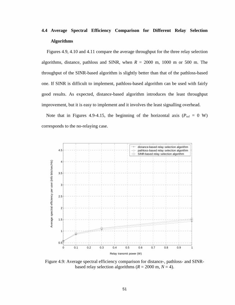
51

4.4 Average Spectral Efficiency Comparison for Different Relay Selection

Algorithms

Figures 4.9, 4.10 and 4.11 compare the average throughput for the three relay selection

algorithms, distance, pathloss and SINR, when R = 2000 m, 1000 m or 500 m. The

throughput of the SINR-based algorithm is slightly better than that of the pathloss-based

one. If SINR is difficult to implement, pathloss-based algorithm can be used with fairly

good results. As expected, distance-based algorithm introduces the least throughput

improvement, but it is easy to implement and it involves the least signalling overhead.

Note that in Figures 4.9-4.15, the beginning of the horizontal axis (Prel = 0 W)

corresponds to the no-relaying case.

0 0.1 0.2 0.3 0.4 0.5 0.6 0.7 0.8 0.9 1

0.5

1

1.5

2

2.5

3

3.5

4

4.5

Relay transmit power (W)

Ave

rage

spe

ctra

l eff

icie

ncy

per

user

(in

fo b

its/s

ec/H

z)

distance-based relay selection algorithmpathloss-based relay selection algorithmSINR-based relay selection algorithm

Figure 4.9: Average spectral efficiency comparison for distance-, pathloss- and SINR-based relay selection algorithms (R = 2000 m, N = 4).

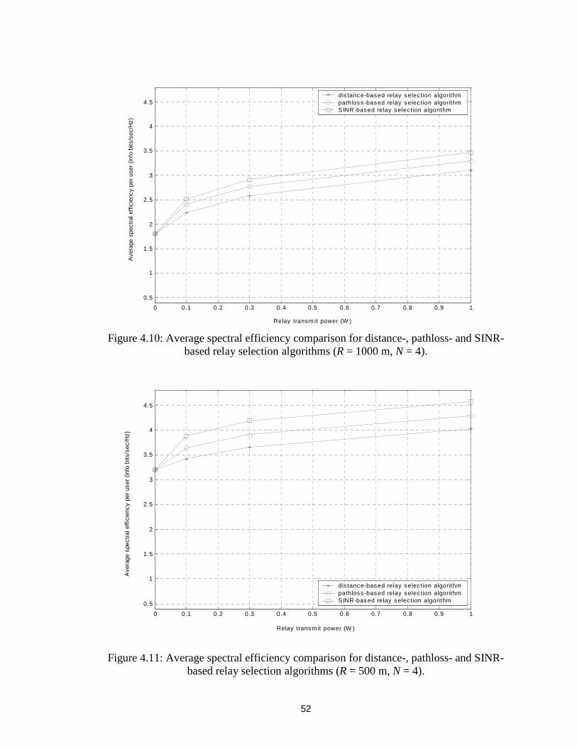
52

0 0.1 0.2 0.3 0.4 0.5 0.6 0.7 0.8 0.9 1

0.5

1

1.5

2

2.5

3

3.5

4

4.5

Relay transm it power (W )

Ave

rage

spe

ctra

l eff

icie

ncy

per

user

(in

fo b

its/s

ec/H

z)

dis tance-based relay selec tion algorithmpathloss -based relay selec tion algorithmSINR-based relay selection algorithm

Figure 4.10: Average spectral efficiency comparison for distance-, pathloss- and SINR-based relay selection algorithms (R = 1000 m, N = 4).

0 0.1 0.2 0.3 0.4 0.5 0.6 0.7 0.8 0.9 1

0.5

1

1.5

2

2.5

3

3.5

4

4.5

Relay transmit power (W )

Ave

rage

spe

ctra

l eff

icie

ncy

per

user

(in

fo b

its/s

ec/H

z)

dis tance-based relay selec tion algorithmpathloss-based relay selec tion algorithmSINR-based relay selection algorithm

Figure 4.11: Average spectral efficiency comparison for distance-, pathloss- and SINR-based relay selection algorithms (R = 500 m, N = 4).

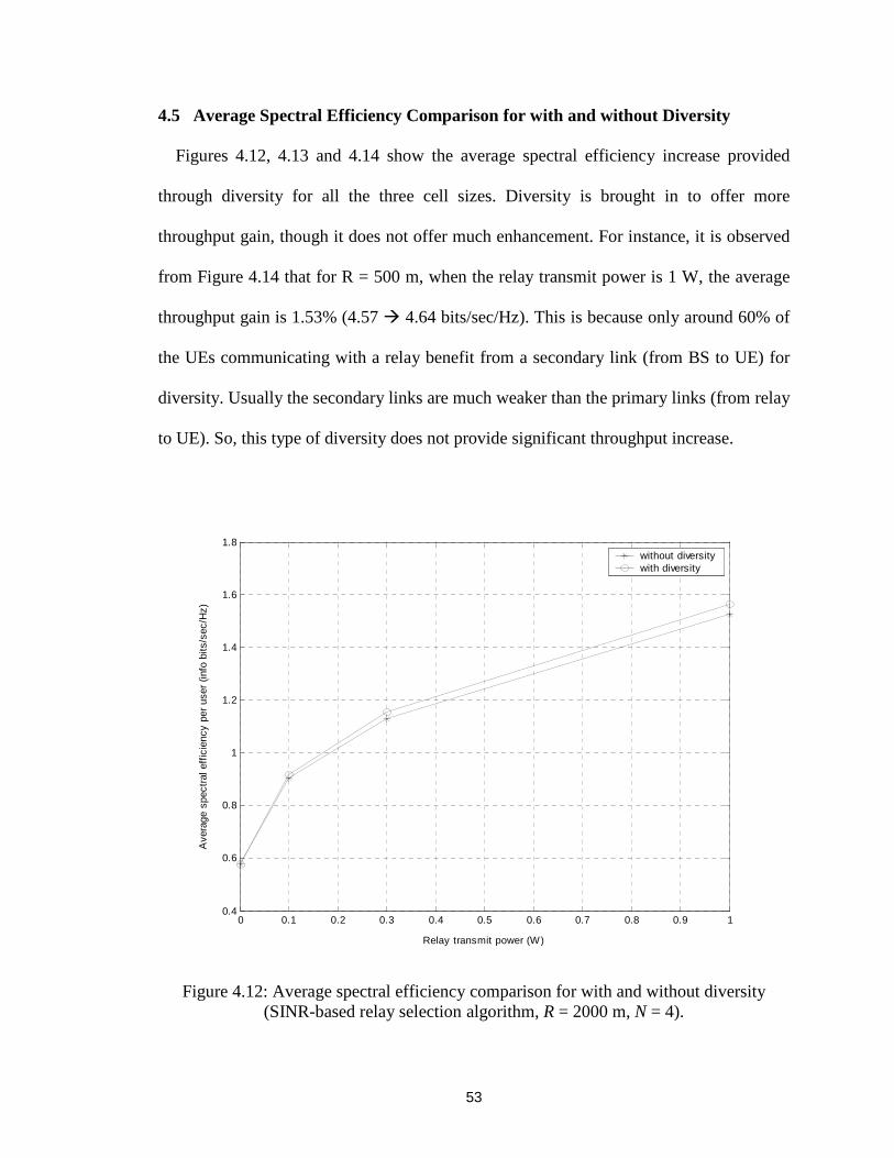
53

4.5 Average Spectral Efficiency Comparison for with and without Diversity

Figures 4.12, 4.13 and 4.14 show the average spectral efficiency increase provided

through diversity for all the three cell sizes. Diversity is brought in to offer more

throughput gain, though it does not offer much enhancement. For instance, it is observed

from Figure 4.14 that for R = 500 m, when the relay transmit power is 1 W, the average

throughput gain is 1.53% (4.57 � 4.64 bits/sec/Hz). This is because only around 60% of

the UEs communicating with a relay benefit from a secondary link (from BS to UE) for

diversity. Usually the secondary links are much weaker than the primary links (from relay

to UE). So, this type of diversity does not provide significant throughput increase.

0 0.1 0.2 0.3 0.4 0.5 0.6 0.7 0.8 0.9 10.4

0.6

0.8

1

1.2

1.4

1.6

1.8

Relay transmit power (W)

Ave

rage

spe

ctra

l eff

icie

ncy

per

user

(in

fo b

its/s

ec/H

z)

without diversitywith diversity

Figure 4.12: Average spectral efficiency comparison for with and without diversity(SINR-based relay selection algorithm, R = 2000 m, N = 4).

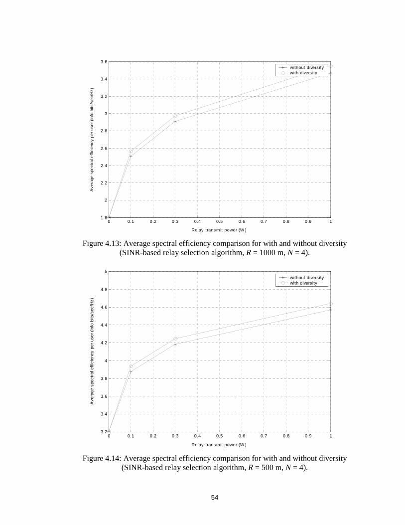
54

0 0.1 0.2 0.3 0.4 0.5 0.6 0.7 0.8 0.9 11.8

2

2.2

2.4

2.6

2.8

3

3.2

3.4

3.6

Relay transmit power (W )

Ave

rage

spe

ctra

l eff

icie

ncy

per

user

(in

fo b

its/s

ec/H

z)

without divers itywith divers ity

Figure 4.13: Average spectral efficiency comparison for with and without diversity(SINR-based relay selection algorithm, R = 1000 m, N = 4).

0 0.1 0.2 0.3 0.4 0.5 0.6 0.7 0.8 0.9 13.2

3.4

3.6

3.8

4

4.2

4.4

4.6

4.8

5

Relay transmit power (W )

Ave

rage

spe

ctra

l eff

icie

ncy

per

user

(in

fo b

its/s

ec/H

z)

without diversitywith diversity

Figure 4.14: Average spectral efficiency comparison for with and without diversity(SINR-based relay selection algorithm, R = 500 m, N = 4).

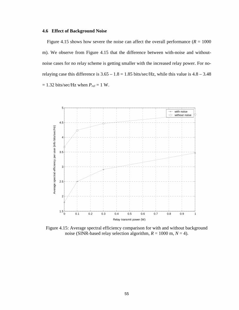
55

4.6 Effect of Background Noise

Figure 4.15 shows how severe the noise can affect the overall performance (R = 1000

m). We observe from Figure 4.15 that the difference between with-noise and without-

noise cases for no relay scheme is getting smaller with the increased relay power. For no-

relaying case this difference is 3.65 – 1.8 = 1.85 bits/sec/Hz, while this value is 4.8 – 3.48

= 1.32 bits/sec/Hz when Prel = 1 W.

0 0.1 0.2 0.3 0.4 0.5 0.6 0.7 0.8 0.9 11.5

2

2.5

3

3.5

4

4.5

5

Relay transmit power (W)

Ave

rage

spe

ctra

l eff

icie

ncy

per

user

(in

fo b

its/s

ec/H

z)

with noisewithout noise

Figure 4.15: Average spectral efficiency comparison for with and without backgroundnoise (SINR-based relay selection algorithm, R = 1000 m, N = 4).

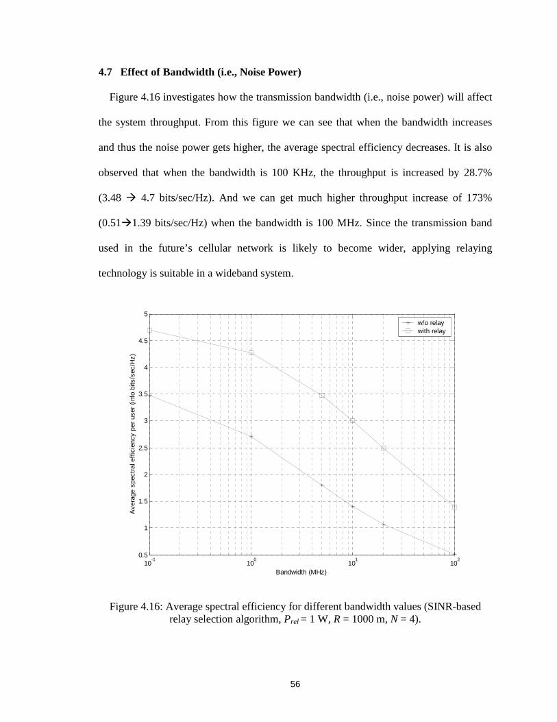
56

4.7 Effect of Bandwidth (i.e., Noise Power)

Figure 4.16 investigates how the transmission bandwidth (i.e., noise power) will affect

the system throughput. From this figure we can see that when the bandwidth increases

and thus the noise power gets higher, the average spectral efficiency decreases. It is also

observed that when the bandwidth is 100 KHz, the throughput is increased by 28.7%

(3.48 � 4.7 bits/sec/Hz). And we can get much higher throughput increase of 173%

(0.51�1.39 bits/sec/Hz) when the bandwidth is 100 MHz. Since the transmission band

used in the future’s cellular network is likely to become wider, applying relaying

technology is suitable in a wideband system.

10-1

100

101

102

0.5

1

1.5

2

2.5

3

3.5

4

4.5

5

Bandwidth (MHz)

Ave

rage

spe

ctra

l eff

icie

ncy

per

user

(in

fo b

its/s

ec/H

z)

w/o relaywith relay

Figure 4.16: Average spectral efficiency for different bandwidth values (SINR-basedrelay selection algorithm, Prel = 1 W, R = 1000 m, N = 4).

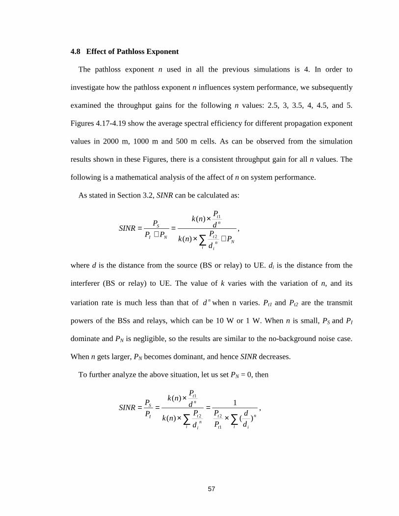
57

4.8 Effect of Pathloss Exponent

The pathloss exponent n used in all the previous simulations is 4. In order to

investigate how the pathloss exponent n influences system performance, we subsequently

examined the throughput gains for the following n values: 2.5, 3, 3.5, 4, 4.5, and 5.

Figures 4.17-4.19 show the average spectral efficiency for different propagation exponent

values in 2000 m, 1000 m and 500 m cells. As can be observed from the simulation

results shown in these Figures, there is a consistent throughput gain for all n values. The

following is a mathematical analysis of the affect of n on system performance.

As stated in Section 3.2, SINR can be calculated as:

Ni

ni

t

nt

NI

S

Pd

Pnk

d

Pnk

PP

PSINR

+×

×=

+=

∑ 2

1

)(

)(,

where d is the distance from the source (BS or relay) to UE. di is the distance from the

interferer (BS or relay) to UE. The value of k varies with the variation of n, and its

variation rate is much less than that of nd when n varies. Pt1 and Pt2 are the transmit

powers of the BSs and relays, which can be 10 W or 1 W. When n is small, PS and PI

dominate and PN is negligible, so the results are similar to the no-background noise case.

When n gets larger, PN becomes dominant, and hence SINR decreases.

To further analyze the above situation, let us set PN = 0, then

∑∑ ×=

×

×==

i

n

it

t

in

i

t

nt

I

S

d

d

P

P

d

Pnk

d

Pnk

P

PSINR

)(

1

)(

)(

1

22

1

,

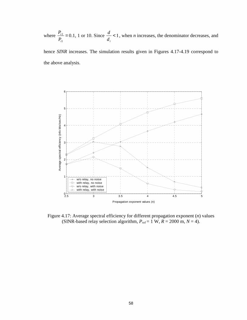
58

where =1

2

t

t

P

P0.1, 1 or 10. Since 1<

id

d, when n increases, the denominator decreases, and

hence SINR increases. The simulation results given in Figures 4.17-4.19 correspond to

the above analysis.

2.5 3 3.5 4 4.5 50

1

2

3

4

5

6

Propagation exponent values (n)

Ave

rage

spe

ctra

l eff

icie

ncy

(info

bits

/sec

/Hz)

w/o relay, no noisewith relay, no noisew/o relay, with noisewith relay, with noise

Figure 4.17: Average spectral efficiency for different propagation exponent (n) values(SINR-based relay selection algorithm, Prel = 1 W, R = 2000 m, N = 4).

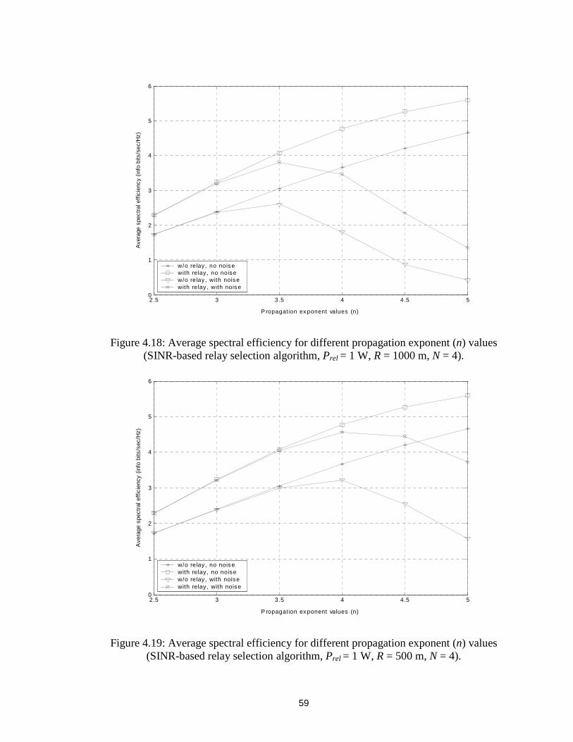
59

2.5 3 3.5 4 4.5 50

1

2

3

4

5

6

P ropagation ex ponent values (n)

Ave

rage

spe

ctra

l eff

icie

ncy

(info

bits

/sec

/Hz)

w/o relay , no nois ewith relay , no nois ew/o relay , with nois ewith relay , with nois e

Figure 4.18: Average spectral efficiency for different propagation exponent (n) values(SINR-based relay selection algorithm, Prel = 1 W, R = 1000 m, N = 4).

2.5 3 3.5 4 4.5 50

1

2

3

4

5

6

P ropagation exponent values (n)

Ave

rage

spe

ctra

l eff

icie

ncy

(info

bits

/sec

/Hz)

w/o relay, no noisewith relay , no noisew/o relay, with noisewith relay , with noise

Figure 4.19: Average spectral efficiency for different propagation exponent (n) values(SINR-based relay selection algorithm, Prel = 1 W, R = 500 m, N = 4).

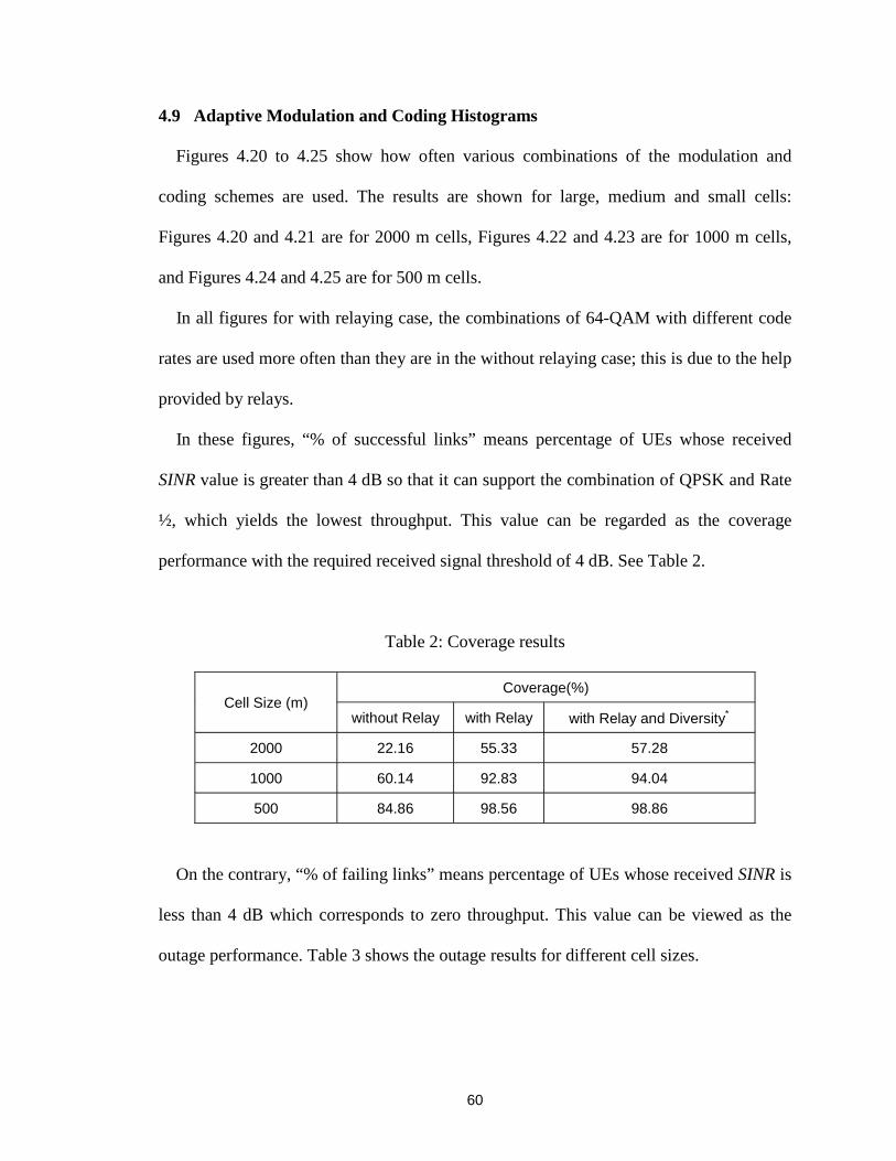
60

4.9 Adaptive Modulation and Coding Histograms

Figures 4.20 to 4.25 show how often various combinations of the modulation and

coding schemes are used. The results are shown for large, medium and small cells:

Figures 4.20 and 4.21 are for 2000 m cells, Figures 4.22 and 4.23 are for 1000 m cells,

and Figures 4.24 and 4.25 are for 500 m cells.

In all figures for with relaying case, the combinations of 64-QAM with different code

rates are used more often than they are in the without relaying case; this is due to the help

provided by relays.

In these figures, “ % of successful links” means percentage of UEs whose received

SINR value is greater than 4 dB so that it can support the combination of QPSK and Rate

½, which yields the lowest throughput. This value can be regarded as the coverage

performance with the required received signal threshold of 4 dB. See Table 2.

Table 2: Coverage results

Coverage(%)Cell Size (m)

without Relay with Relay with Relay and Diversity∗

2000 22.16 55.33 57.28

1000 60.14 92.83 94.04

500 84.86 98.56 98.86

On the contrary, “ % of failing links” means percentage of UEs whose received SINR is

less than 4 dB which corresponds to zero throughput. This value can be viewed as the

outage performance. Table 3 shows the outage results for different cell sizes.

61

Table 3: Outage results

Outage(%)Cell Size (m)

without Relay with Relay with Relay and Diversity∗

2000 77.84 44.67 42.72

1000 39.86 7.17 5.96

500 15.14 1.44 1.14

QPSK

16-QAM

64-QAM

Rate:1/2

Rate:2/3

Rate:3/4

Rate:7/8

Rate:1

0%

2%

4%

6%

8%

10%

code rate

modulation

% o

f tim

e fo

r us

ing

a co

mbi

natio

n of

mod

ulat

ion

and

codi

ng

% of successful links: 22.16

% of failing links: 77.84

Figure 4.20: Percentage of time using a combination of modulation and coding (withoutrelaying, SINR-based relay selection algorithm, R = 2000 m, N = 4).

∗ The data in this column is read from the histograms in Appendix C.

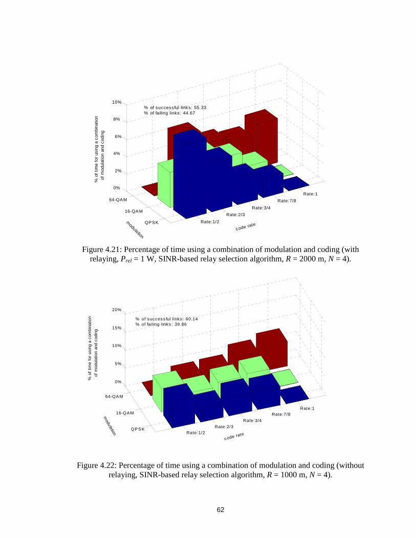
62

QPSK

16-QAM

64-QAM

Rate:1/2

Rate:2/3

Rate:3/4

Rate:7/8

Rate:10%

2%

4%

6%

8%

10%

code ratem

odulation

% o

f tim

e fo

r us

ing

a co

mbi

natio

n of

mod

ulat

ion

and

codi

ng

% of successful links: 55.33% of failing links: 44.67

Figure 4.21: Percentage of time using a combination of modulation and coding (withrelaying, Prel = 1 W, SINR-based relay selection algorithm, R = 2000 m, N = 4).

QPSK

16-QAM

64-QA M

Rate:1/2Rate:2/3

Rate:3/4

Rate:7/8Rate:1

0%

5%

10%

15%

20%

code rate

modulation

% o

f tim

e fo

r us

ing

a co

mbi

natio

n o

f m

odul

atio

n an

d co

ding

% of success ful links : 60.14

% of failing links : 39.86

Figure 4.22: Percentage of time using a combination of modulation and coding (withoutrelaying, SINR-based relay selection algorithm, R = 1000 m, N = 4).

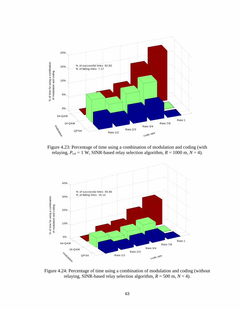
63

QPSK

16-QAM

64-QAM

Rate:1/2Rate:2/3

Rate:3/4Rate:7/8

Rate:1

0%

5%

10%

15%

20%

code rate

modulation

% o

f tim

e fo

r us

ing

a co

mbi

natio

n of

mod

ulat

ion

and

codi

ng

% of successful links: 92.83% of failing links: 7.17

Figure 4.23: Percentage of time using a combination of modulation and coding (withrelaying, Prel = 1 W, SINR-based relay selection algorithm, R = 1000 m, N = 4).

QPSK

16-QAM

64-QAM

Rate:1/2Rate:2/3

Rate:3/4

Rate:7/8Rate:1

0%

10%

20%

30%

40%

code ratem

odulation

% o

f tim

e fo

r us

ing

a co

mbi

natio

n of

mod

ulat

ion

and

codi

ng

% of successful links: 84.86% of failing links: 15.14

Figure 4.24: Percentage of time using a combination of modulation and coding (withoutrelaying, SINR-based relay selection algorithm, R = 500 m, N = 4).

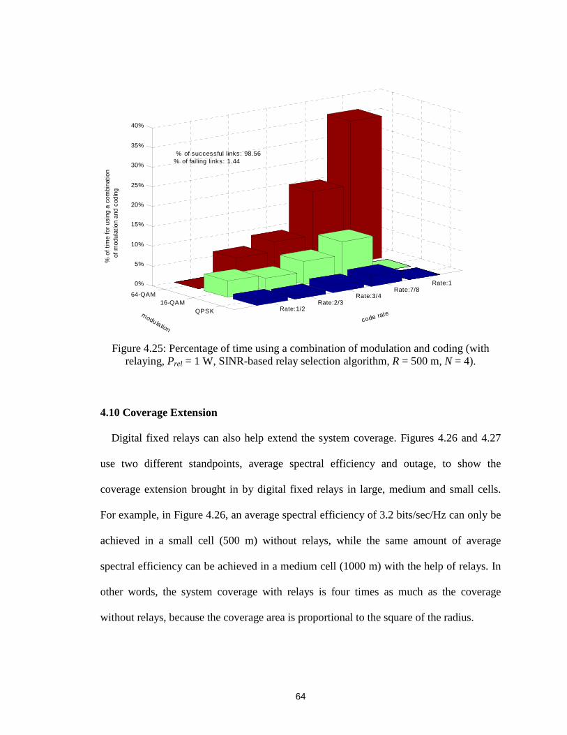
64

QPSK16-QAM

64-QAM

Rate:1/2Rate:2/3

Rate:3/4Rate:7/8

Rate:10%

5%

10%

15%

20%

25%

30%

35%

40%

code ratemodulation

% o

f tim

e fo

r us

ing

a co

mbi

natio

n o

f m

odul

atio

n an

d co

ding

% of successful links: 98.56% of failing links: 1.44

Figure 4.25: Percentage of time using a combination of modulation and coding (withrelaying, Prel = 1 W, SINR-based relay selection algorithm, R = 500 m, N = 4).

4.10 Coverage Extension

Digital fixed relays can also help extend the system coverage. Figures 4.26 and 4.27

use two different standpoints, average spectral efficiency and outage, to show the

coverage extension brought in by digital fixed relays in large, medium and small cells.

For example, in Figure 4.26, an average spectral efficiency of 3.2 bits/sec/Hz can only be

achieved in a small cell (500 m) without relays, while the same amount of average

spectral efficiency can be achieved in a medium cell (1000 m) with the help of relays. In

other words, the system coverage with relays is four times as much as the coverage

without relays, because the coverage area is proportional to the square of the radius.

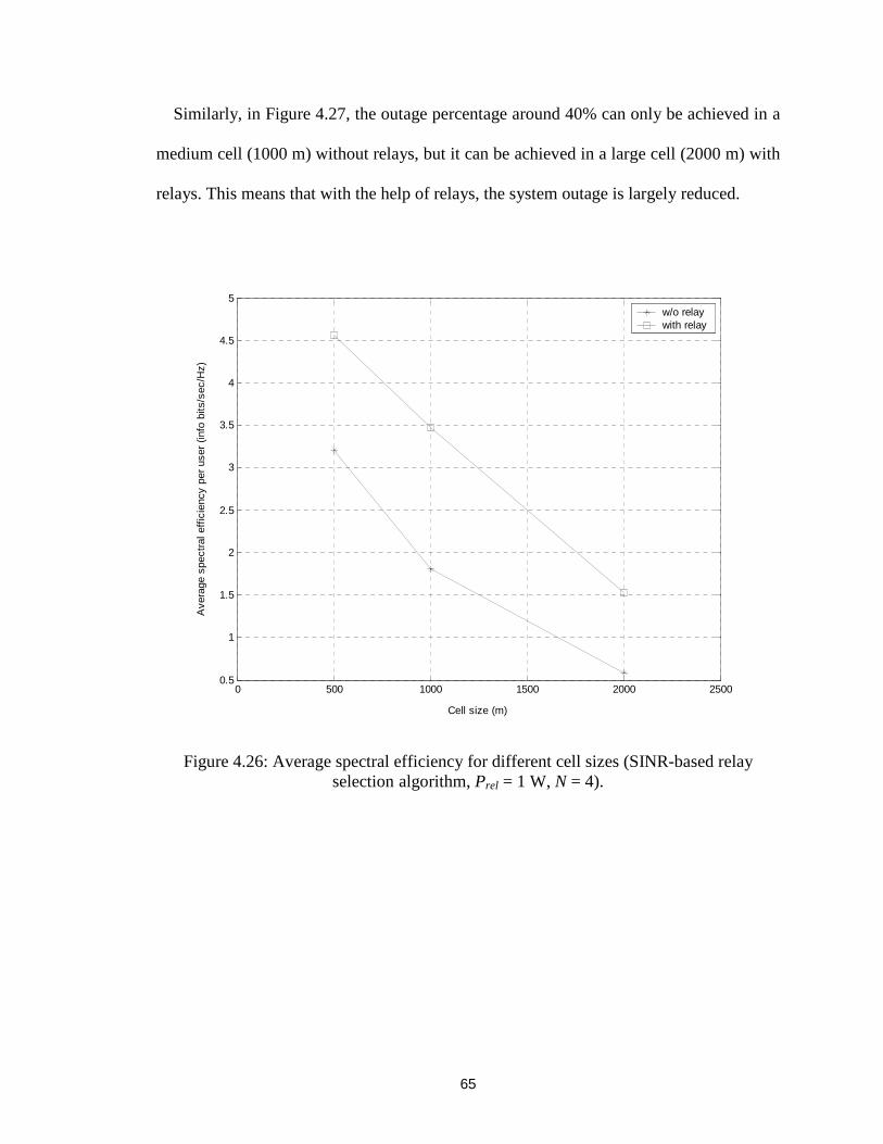
65

Similarly, in Figure 4.27, the outage percentage around 40% can only be achieved in a

medium cell (1000 m) without relays, but it can be achieved in a large cell (2000 m) with

relays. This means that with the help of relays, the system outage is largely reduced.

0 500 1000 1500 2000 25000.5

1

1.5

2

2.5

3

3.5

4

4.5

5

Cell size (m)

Ave

rage

spe

ctra

l eff

icie

ncy

per

user

(in

fo b

its/s

ec/H

z)

w/o relaywith relay

Figure 4.26: Average spectral efficiency for different cell sizes (SINR-based relayselection algorithm, Prel = 1 W, N = 4).

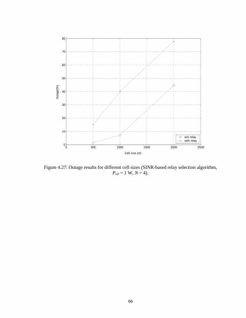
66

0 500 1000 1500 2000 25000

10

20

30

40

50

60

70

80

Cell size (m)

Out

age(

%)

w/o relaywith relay

Figure 4.27: Outage results for different cell sizes (SINR-based relay selection algorithm,Prel = 1 W, N = 4).

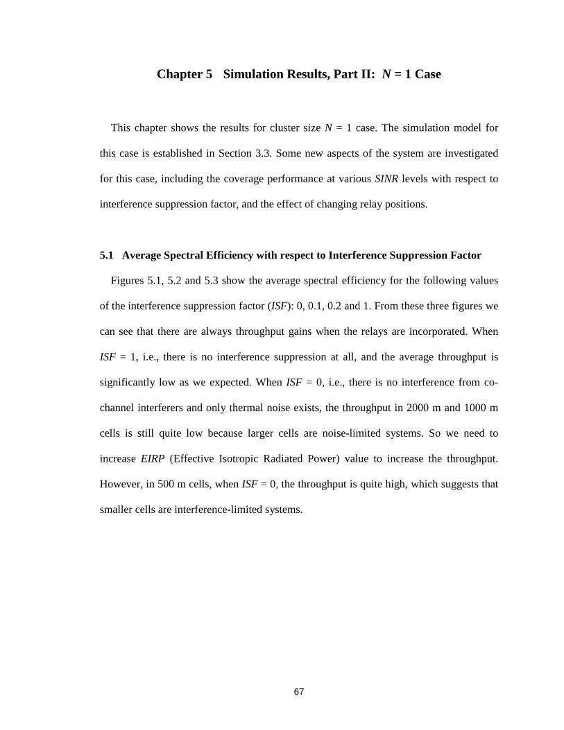
67

Chapter 5 Simulation Results, Part II: N = 1 Case

This chapter shows the results for cluster size N = 1 case. The simulation model for

this case is established in Section 3.3. Some new aspects of the system are investigated

for this case, including the coverage performance at various SINR levels with respect to

interference suppression factor, and the effect of changing relay positions.

5.1 Average Spectral Efficiency with respect to Interference Suppression Factor

Figures 5.1, 5.2 and 5.3 show the average spectral efficiency for the following values

of the interference suppression factor (ISF): 0, 0.1, 0.2 and 1. From these three figures we

can see that there are always throughput gains when the relays are incorporated. When

ISF = 1, i.e., there is no interference suppression at all, and the average throughput is

significantly low as we expected. When ISF = 0, i.e., there is no interference from co-

channel interferers and only thermal noise exists, the throughput in 2000 m and 1000 m

cells is still quite low because larger cells are noise-limited systems. So we need to

increase EIRP (Effective Isotropic Radiated Power) value to increase the throughput.

However, in 500 m cells, when ISF = 0, the throughput is quite high, which suggests that

smaller cells are interference-limited systems.

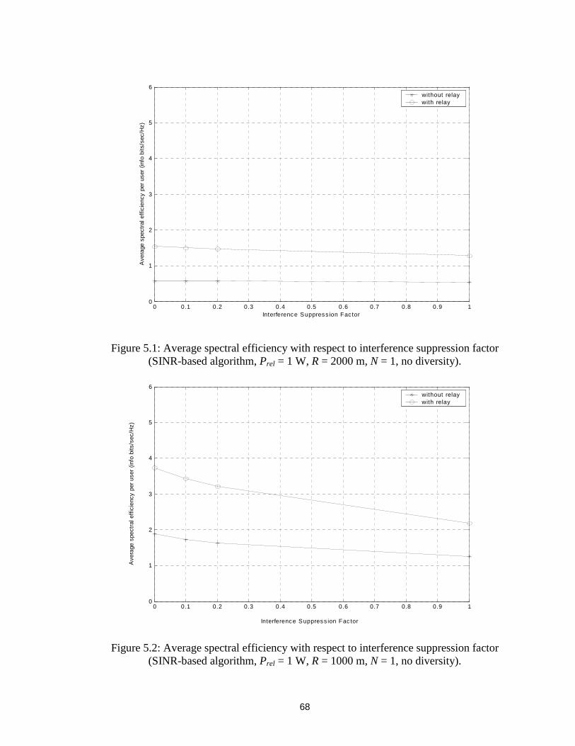
68

0 0.1 0.2 0.3 0.4 0.5 0.6 0.7 0.8 0.9 10

1

2

3

4

5

6

Interference Suppress ion Fac tor

Ave

rage

spe

ctra

l eff

icie

ncy

per

user

(in

fo b

its/s

ec/H

z)

without relaywith relay

Figure 5.1: Average spectral efficiency with respect to interference suppression factor(SINR-based algorithm, Prel = 1 W, R = 2000 m, N = 1, no diversity).

0 0.1 0.2 0.3 0.4 0.5 0.6 0.7 0.8 0.9 10

1

2

3

4

5

6

Interference Suppress ion Fac tor

Ave

rage

spe

ctra

l eff

icie

ncy

per

user

(in

fo b

its/s

ec/H

z)

without relaywith relay

Figure 5.2: Average spectral efficiency with respect to interference suppression factor(SINR-based algorithm, Prel = 1 W, R = 1000 m, N = 1, no diversity).

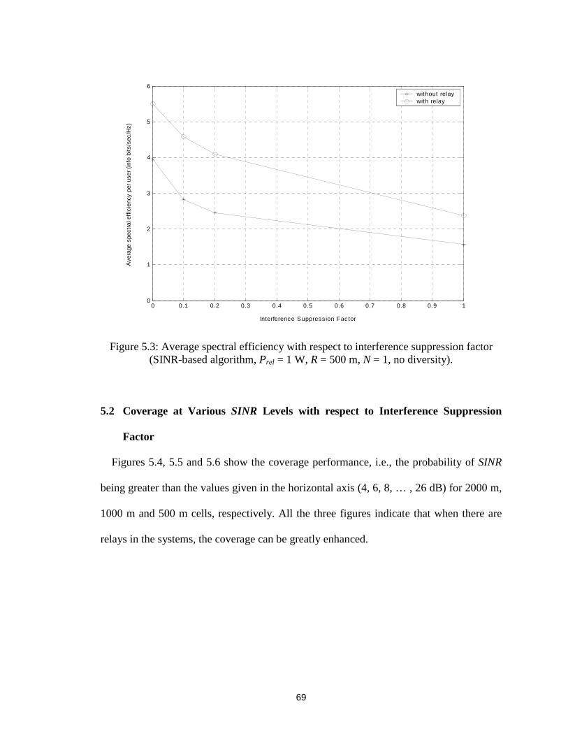
69

0 0.1 0.2 0.3 0.4 0.5 0.6 0.7 0.8 0.9 10

1

2

3

4

5

6

Interference Suppression Fac tor

Ave

rage

spe

ctra

l eff

icie

ncy

per

user

(in

fo b

its/s

ec/H

z)

without relaywith relay

Figure 5.3: Average spectral efficiency with respect to interference suppression factor(SINR-based algorithm, Prel = 1 W, R = 500 m, N = 1, no diversity).

5.2 Coverage at Various SINR Levels with respect to Interference Suppression

Factor

Figures 5.4, 5.5 and 5.6 show the coverage performance, i.e., the probability of SINR

being greater than the values given in the horizontal axis (4, 6, 8, … , 26 dB) for 2000 m,

1000 m and 500 m cells, respectively. All the three figures indicate that when there are

relays in the systems, the coverage can be greatly enhanced.

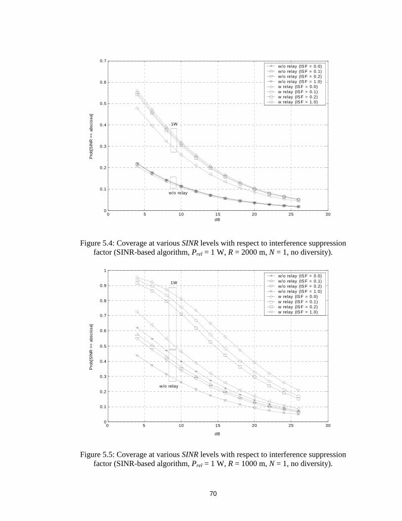
70

0 5 10 15 20 25 300

0.1

0.2

0.3

0.4

0.5

0.6

0.7

Pro

b[S

INR

>=

abs

ciss

a]

dB

w/o relay (IS F = 0.0)w/o relay (IS F = 0.1)w/o relay (IS F = 0.2)w/o relay (IS F = 1.0)w relay (ISF = 0.0)w relay (ISF = 0.1)w relay (ISF = 0.2)w relay (ISF = 1.0)

1W

w/o relay

Figure 5.4: Coverage at various SINR levels with respect to interference suppressionfactor (SINR-based algorithm, Prel = 1 W, R = 2000 m, N = 1, no diversity).

0 5 10 15 20 25 300

0.1

0.2

0.3

0.4

0.5

0.6

0.7

0.8

0.9

1

Pro

b[S

INR

>=

abs

ciss

a]

dB

w/o relay (IS F = 0.0)w/o relay (IS F = 0.1)w/o relay (IS F = 0.2)w/o relay (IS F = 1.0)w relay (ISF = 0.0)w relay (ISF = 0.1)w relay (ISF = 0.2)w relay (ISF = 1.0)

1W

w/o relay

Figure 5.5: Coverage at various SINR levels with respect to interference suppressionfactor (SINR-based algorithm, Prel = 1 W, R = 1000 m, N = 1, no diversity).

71

0 5 10 15 20 25 300

0.1

0.2

0.3

0.4

0.5

0.6

0.7

0.8

0.9

1

Pro

b[S

INR

>=

abs

ciss

a]

dB

w/o relay (ISF = 0.0)w/o relay (ISF = 0.1)w/o relay (ISF = 0.2)w/o relay (ISF = 1.0)w relay (ISF = 0.0)w relay (ISF = 0.1)w relay (ISF = 0.2)w relay (ISF = 1.0)

Figure 5.6: Coverage at various SINR levels with respect to interference suppressionfactor (SINR-based algorithm, Prel = 1 W, R = 500 m, N = 1, no diversity).

5.3 Average Spectral Efficiency with respect to Relay Positions

Figure 5.8 shows the average spectral efficiency with respect to the relay positions for

1000 m and 500 m cells. As discussed in Section 2.3, the relays are placed on the

segment between the centre and one corner of that cell. Here the relay position is

indicated by a parameter m showing how far away the relay is from the BS. Please refer

to Figure 5.7.

R

am = ,

where a is the distance from the BS to the relay, R is the distance from the BS to one

corner of the cell. In the simulation, the following m values are examined: 0, 0.1, 0.2, … ,

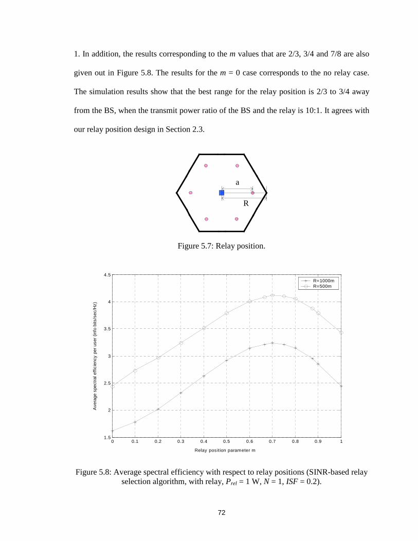
72

1. In addition, the results corresponding to the m values that are 2/3, 3/4 and 7/8 are also

given out in Figure 5.8. The results for the m = 0 case corresponds to the no relay case.

The simulation results show that the best range for the relay position is 2/3 to 3/4 away

from the BS, when the transmit power ratio of the BS and the relay is 10:1. It agrees with

our relay position design in Section 2.3.

a

R

Figure 5.7: Relay position.

0 0.1 0.2 0.3 0.4 0.5 0.6 0.7 0.8 0.9 11.5

2

2.5

3

3.5

4

4.5

Relay position parameter m

Ave

rage

spe

ctra

l eff

icie

ncy

per

user

(in

fo b

its/s

ec/H

z)

R=1000mR=500m

Figure 5.8: Average spectral efficiency with respect to relay positions (SINR-based relayselection algorithm, with relay, Prel = 1 W, N = 1, ISF = 0.2).

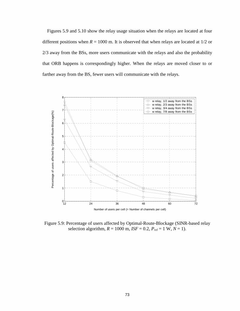
73

Figures 5.9 and 5.10 show the relay usage situation when the relays are located at four

different positions when R = 1000 m. It is observed that when relays are located at 1/2 or

2/3 away from the BSs, more users communicate with the relays and also the probability

that ORB happens is correspondingly higher. When the relays are moved closer to or

farther away from the BS, fewer users will communicate with the relays.

12 24 36 48 60 720

1

2

3

4

5

6

7

8

Number of users per cell (= Number of channels per cell)

Per

cent

age

of u

sers

aff

ecte

d by

Opt

imal

-Rou

te-B

lock

age(

%)

w relay, 1/2 away from the BSsw relay, 2/3 away from the BSsw relay, 3/4 away from the BSsw relay, 7/8 away from the BSs

Figure 5.9: Percentage of users affected by Optimal-Route-Blockage (SINR-based relayselection algorithm, R = 1000 m, ISF = 0.2, Prel = 1 W, N = 1).

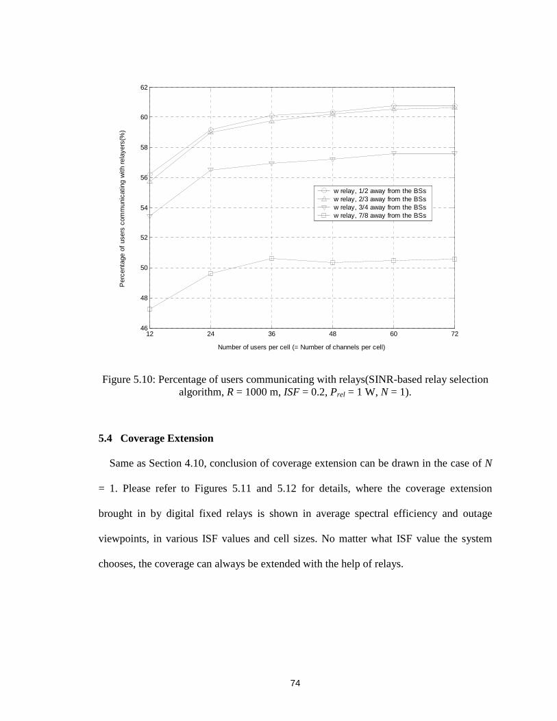
74

12 24 36 48 60 7246

48

50

52

54

56

58

60

62

Number of users per cell (= Number of channels per cell)

Per

cent

age

of u

sers

com

mun

icat

ing

with

rel

ayer

s(%

)

w relay, 1/2 away from the BSsw relay, 2/3 away from the BSsw relay, 3/4 away from the BSsw relay, 7/8 away from the BSs

Figure 5.10: Percentage of users communicating with relays(SINR-based relay selectionalgorithm, R = 1000 m, ISF = 0.2, Prel = 1 W, N = 1).

5.4 Coverage Extension

Same as Section 4.10, conclusion of coverage extension can be drawn in the case of N

= 1. Please refer to Figures 5.11 and 5.12 for details, where the coverage extension

brought in by digital fixed relays is shown in average spectral efficiency and outage

viewpoints, in various ISF values and cell sizes. No matter what ISF value the system

chooses, the coverage can always be extended with the help of relays.

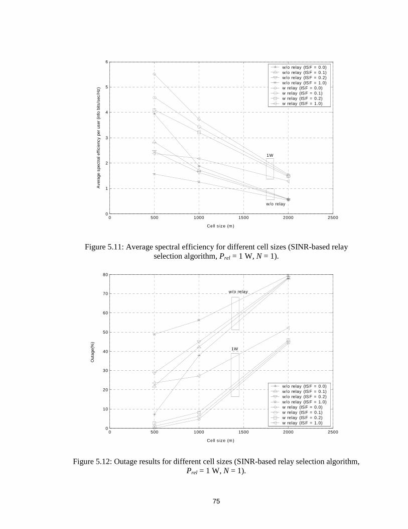
75

0 500 1000 1500 2000 25000

1

2

3

4

5

6

Cell s ize (m)

Ave

rage

spe

ctra

l eff

icie

ncy

per

user

(in

fo b

its/s

ec/H

z)

w/o relay (IS F = 0.0)w/o relay (IS F = 0.1)w/o relay (IS F = 0.2)w/o relay (IS F = 1.0)w relay (ISF = 0.0)w relay (ISF = 0.1)w relay (ISF = 0.2)w relay (ISF = 1.0)

1W

w/o relay

Figure 5.11: Average spectral efficiency for different cell sizes (SINR-based relayselection algorithm, Prel = 1 W, N = 1).

0 500 1000 1500 2000 25000

10

20

30

40

50

60

70

80

Cell s ize (m)

Out

age(

%)

w/o relay (IS F = 0.0)w/o relay (IS F = 0.1)w/o relay (IS F = 0.2)w/o relay (IS F = 1.0)w relay (ISF = 0.0)w relay (ISF = 0.1)w relay (ISF = 0.2)w relay (ISF = 1.0)

1W

w/o relay

Figure 5.12: Outage results for different cell sizes (SINR-based relay selection algorithm,Prel = 1 W, N = 1).

76

Chapter 6 Conclusions and Discussions

6.1 Conclusions

This research studies the possible benefits that digital fixed relaying technology is able

to provide for current and future cellular mobile networks. From the simulation results,

we can conclude that digital fixed relaying is a simple yet effective approach to improve

system throughput and high data rate coverage. Here are our observations:

First of all, in the new proposed network infrastructure, channel reuse is even denser

due to the fact that the relaying channels are acquired through the reuse of existing

channels, which will subsequently cause extra interference. However, simulation results

still show that there are throughput improvements even if this extra interference is taken

into account. Another point worth mentioning is the following: the simulation results

indicate that with this relaying channel reuse design, ORB happens infrequently.

Secondly, the highest AMC combination utilized in this simulation is 64-QAM with

code rate 1, corresponding to 6 bits/sec/Hz. As shown in the histograms 4.23 and 4.25 in

Chapter 4, with the incorporation of relaying, the average received SINR by a UE is

increased and therefore, the majority percentage of UEs are using the highest AMC

combination. As can be imagined, there must be UEs whose receiving SINR is much

higher than 26 dB, which are limited to use the combination of 64-QAM and code rate 1.

And it can be anticipated that better results can be achieved when implementing higher

AMC levels, for example 128-QAM and various code rate for these UEs. This is

especially the case for small cells. So for nomadic applications in small cells, using

higher AMC levels is recommended.

77

Thirdly, regarding the three relay selection algorithms, the advantages and

disadvantages are analyzed thoroughly for each of them. The distance-based algorithm is

the easiest to implement with the assistance of GPS (Global Positioning System)

technology, but it brings in the least throughput increase; the SINR-based algorithm

produces the greatest throughput improvement, however it involves more signalling

overheads; the performance of the pathloss-based algorithm works in the middle.

Furthermore, as far as the relay position is concerned, we can tell from the simulation

results that the best performance can be attained with the placement of relays at 2/3 to 3/4

away from the BS, when the transmit power ratio of the BS and the relay is 10:1. Nearer

or farther from the BS will weaken the SINR values.

Moreover, two-path diversity is incorporated in the SINR-based algorithm and this

proves that a further throughput increase can be obtained but at a very modest level. It is

worth pointing out that diversity does not require any extra bandwidth or transmit power.

Two different cell cluster sizes, N = 1 and N = 4, are investigated as well. It can be

concluded that digital fixed relaying technology works well in both cases.

Various values are applied to the pathloss propagation exponent n, i.e., 2.5, 3, 3.5, 4,

4.5 and 5. For all values of n, throughput improvements are observed consistently with

the implementation of digital fixed relays.

6.2 Thesis Contributions

This section provides a summary of various highlights that contribute to this thesis.

• A proposal of a novel cellular infrastructure with the addition of digital fixed relays in

the conventional cellular networks, along with three relay selection schemes and a

78

pre-configured relaying channel partition scheme to be used for relaying channel

selection which can be applied to any cluster sizes. This is the primary contribution of

this thesis.

• A series of simulations that support the intuitive idea provided in this thesis that

digital fixed relaying technology coupled with the adoption of AMC scheme

enhances the throughput and coverage of the cellular networks and realize the

ubiquitous high data rate coverage in the entire network.

• A simulation comparison among different relay selection algorithms.

• A simulation to show that incorporating diversity can further increase the system

throughput and coverage, though not much.

• A simulation to verify that digital fixed relays work well for both cluster size N = 4

and N = 1 cases and for various system parameters (propagation exponents, cell sizes,

relay locations, etc.)

6.3 Future Research

This research opens up a series of interesting subjects for future work:

1. Load balancing is another possible benefit that digital fixed relays might be able

to offer. When the traffic in a certain BS is overloaded, the relay may be able to

divert an amount of traffic to the neighbouring BSs with extra resources, and thus

the entire traffic load is well balanced.

2. The digital fixed relaying in this research is a two-hop technology, which raises a

possible future research of exploring the advantages and disadvantages of digital

79

fixed relaying with more than two hops, i.e., the multi-hop digital fixed relaying

technology.

3. The relaying channel partition scheme in this research is solely based on

pessimistic assumptions: no existing radio channels can be reserved for relaying

purpose. However, if sometimes the radio resources are abundant, one may

consider reserving a part of radio channels for relaying channels, and ascertain the

advantages and shortcomings it may generate.

4. The two-path diversity is employed in this research. Other diversity techniques

may also be considered in future research to bring unique advantages to the

system performance.

5. The study of digital fixed relaying for UEs when they are in mobility is another

key research area.

6. Antenna techniques have advanced rapidly in recent years. The investigation of

digital fixed relaying combined with different antenna techniques is

recommended as well.

7. This research is focused on the benefits that digital fixed relaying can provide for

circuit switched data, i.e., data transferred in continuous queues, but we notice

that packet switched data has been highly demanded in modern cellular networks

as well. Packet switched data happens when data are transferred in large packets

or bursts, and it is suitable for large amounts of data transmission. The study of

how digital fixed relaying can serve packet switched data transmission will

definitely be a promising subject.

80

References

[1] Y. D. Lin and Y. C. Hsu, “ Multihop cellular: a new architecture for wireless

communications” , IEEE INFOCOM’00, pp. 1273-1282, 2000.

[2] M. O. Hasna and M. Alouini, “ Performance analysis of two-hop relayed

transmissions over Rayleigh fading channels” , IEEE 56th Vehicular Technology

Conference (VTC’02), pp. 1992-1996, 2002.

[3] H. Wu, C. Qiao, S. De and O. Tonguz, “ Integrated cellular and ad hoc relaying

systems: iCAR” , IEEE Journal on Selected Areas in Communications (JSAC), vol.

19, no. 10, pp. 2105-2115, October 2001.

[4] V. Sreng, “ Coverage Enhancement through Two-Hop Relaying in Cellular Radio

Systems” , M.A.Sc. Thesis, supervisors: H. Yanikomeroglu and D. D. Falconer,

Carleton University, 2002.

[5] H. Yanikomeroglu, “ Fixed and mobile relaying technologies for cellular networks” ,

Second Workshop on Applications and Services in Wireless Networks (ASWN'02),

pp. 75-81, July 2002.

[6] E. Armanious, D. D. Falconer, and H. Yanikomeroglu, “ Adaptive modulation,

adaptive coding, and power control for fixed cellular broadband wireless systems” ,

IEEE Wireless Communications and Networking Conference (WCNC'03), March

2003.

[7] G. Cair, G. Taricco, and E. Biglieri, “ Bit-interleaved coded modulation,” IEEE

Trans. Info. Theory, vol. 44, no. 3, pp. 927-946, May 1998.

81

[8] V. Sreng, H. Yanikomeroglu, and D. D. Falconer “ Capacity enhancement through

two-hop relaying in cellular radio systems” , IEEE Wireless Communications and

Networking Conference (WCNC’02), 2002.

[9] T. S. Rappaport, Wireless Communications: Principles and Practice, Prentice Hall

PTR, 2002.

[10] X. Tang, “ Coverage Enhancement with Analog Fixed Relaying in Cellular Radio

Networks” , M.A.Sc. Thesis, supervisor: D. D. Falconer, Carleton University, 2003.

[11] C. Qiao, H. Wu, and O. Tonguz, “ Load balancing via relay in next generation

wireless systems,” Proc. of Mobile and Ad Hoc Networking and Computing

Conference, 2000.

[12] T. S. Rappaport, et. al, “ Position Location Using Wireless Communications on

Highways of the Future,” IEEE Communications Magazine, pp. 30-37, Oct. 1996.

[13] J. H. Reed, et. al, “ An Overview of the Challenges and Progress in Meeting the E-

911 Requirement for Location Service,” IEEE Communications Magazine, pp. 30-

37, Apr. 1998.

[14] E. Zehavi, “ 8-PSK trellis codes for a Rayleigh channel,” IEEE Trans. Commun., vol.

40, pp. 873-884, May 1992.

[15] S. Y. Le Goff, “ Signal Constellations for Bit-Interleaved Coded Modulation” , IEEE

Trans. Info. Theory, vol. 49, no. 3, May 1998.

[16] D. Walsh, “ Relaying Using the Unlicensed Bands in Cellular CDMA Networks” ,

M.A.Sc. Thesis in progress, supervisor: H.Yanikomeroglu, Carleton University.

82

[17] Branimir Vojcic, Raymond Pickholtz, Dezso Vekasky and Michael Souryal,

“ Throughput Analysis of Cellular Multihop Networks” , report submitted to Nortel

Networks.

[18] J. Boyer, “ Multihop Wireless Communications Channels” , M.A.Sc. Thesis,

supervisor: D. D. Falconer and H. Yanikomeroglu, Carleton University, 2001.

[19] S. Hares, H. Yanikomeroglu, and B. Hashem, “ A relaying algorithm for multihop

TDMA TDD networks using diversity” , accepted to IEEE Vehicular Technology

Conference, October 2003.

[20] E. Armanious, “ Link adaptation techniques for cellular fixed broadband wireless

access” , M.A.Sc. Thesis, supervisor: H. Yanikomeroglu and D. D. Falconer,

Carleton University, 2003.

[21] A. Sendonaris, E. Erkip, and B. Aazhang, “ User Cooperation Diversity – Parts I and

II,” to appear in IEEE Trans. on Communications.

[22] J. Boyer, D. D. Falconer, and H. Yanikomeroglu, “ A theoretical characterization of

the multihop wireless communications channel with diversity” , IEEE Globecom,

2001.

[23] J. Boyer, D. Falconer, and H. Yanikomeroglu, “ Multihop wireless communications

channels” , submitted to IEEE Transactions on Communications, April 2003.

[24] J. Boyer, D. D. Falconer, and H. Yanikomeroglu, “ A theoretical characterization of

the multihop wireless communications channel without diversity” , IEEE Int.’ l

Symposium on Personal, Indoor, and Mobile Radio Communications (PIMRC),

2001.

83

[25] S. Nanda, K. Balachandran, and S. Kumar, “ Adaptation techniques in wireless

packet data services” , IEEE Communications Magazine, vol. 38, no. 1, pp. 54-64,

Jan. 2000.

[26] A. Goldsmisth and S. G. Chua, “ Adaptive coded modulation for fading channels” ,

IEEE Transactions on Communications, vol. 46, no. 5, pp. 595-602, May 1998.

[27] K. Balachandran, S. R. Kadaba, and S. Nanda, “ Channel quality estimation and rate

adaptation for cellular mobile radio” , IEEE Journal in Selected Areas Commun., vol.

17, no. 7, pp. 1244-1256, July. 1999.

[28] M. Turkboylari and G. L. Stuber, “ An efficient algorithm for estimating the signal-

to-interference ratio in TDMA cellular systems” , IEEE Trans. Commun., vol. 46, no.

6, pp. 728-731, July 1998.

[29] H. Yanikomeroglu, D. D. Falconer, and V. M. Sreng, “ Coverage enhancement

through two-hop peer-to-peer relaying in cellular radio networks” , World Wireless

Research Forum (WWRF) meeting no. 7, Dec. 2002.

[30] V. Sreng, H. Yanikomeroglu, D. Falconer, “ Coverage enhancement through peer-to-

peer relaying in cellular networks’, submitted to IEEE Transactions on Wireless

Communications, Sept. 2002.

[31] V. Sreng, H. Yanikomeroglu, D. Falconer, “ Peer selection strategies in peer-to-peer

relaying in cellular networks” , accepted to IEEE Vehicular Technology Conference,

Fall, 2003.

[32] S. Hares, H. Yanikomeroglu, and B. Hashem, “ Multihop relaying with diversity in

peer-to-peer networks” , accepted to IEEE Globecom, December 2003.

84

Appendix A - Geometric Characteristic of Co-channel BSs and Relays for ClusterSize N = 3 and N = 7 Cases________________________________________________________________________

Figure A.1: Cluster size N = 3 case.

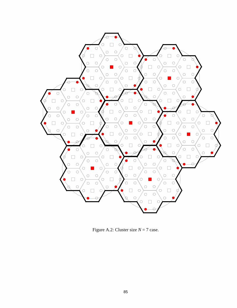
85

Figure A.2: Cluster size N = 7 case.

6C

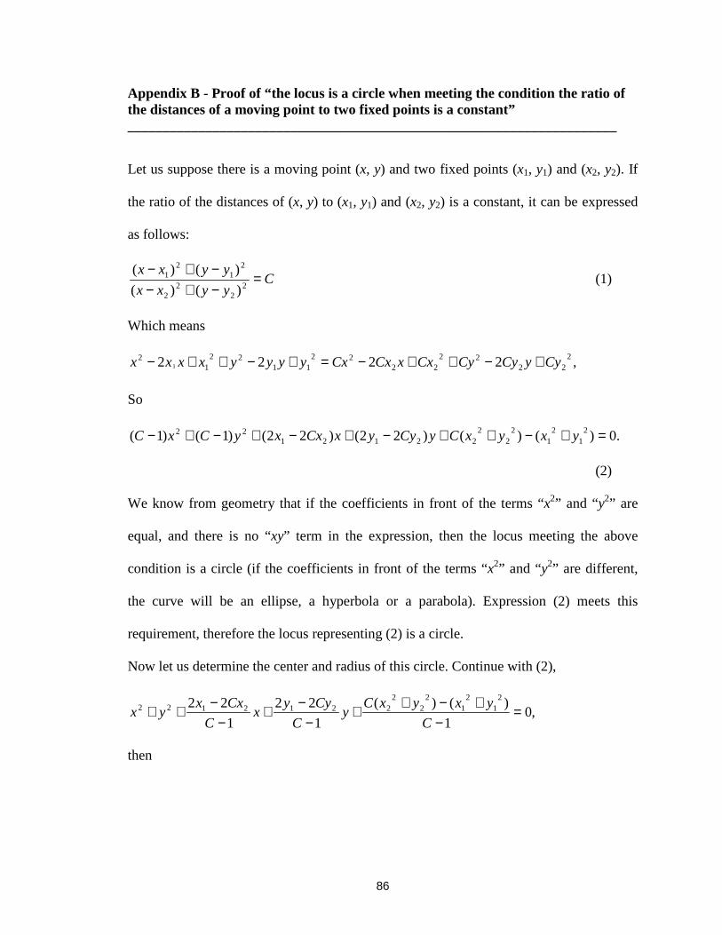
86

Appendix B - Proof of “the locus is a circle when meeting the condition the ratio ofthe distances of a moving point to two fixed points is a constant”_____________________________________________________________________

Let us suppose there is a moving point (x, y) and two fixed points (x1, y1) and (x2, y2). If

the ratio of the distances of (x, y) to (x1, y1) and (x2, y2) is a constant, it can be expressed

as follows:

Cyyxx

yyxx=

−+−−+−

22

22

21

21

)()(

)()( (1)

Which means

,2222 222

2222

2211

221

21 CyyCyCyCxxCxCxyyyyxxxx +−++−=+−++−

So

.0)()()22()22()1()1( 21

21

22

222121

22 =+−++−+−+−+− yxyxCyCyyxCxxyCxC

(2)

We know from geometry that if the coefficients in front of the terms “ x2” and “ y2” are

equal, and there is no “ xy” term in the expression, then the locus meeting the above

condition is a circle (if the coefficients in front of the terms “ x2” and “ y2” are different,

the curve will be an ellipse, a hyperbola or a parabola). Expression (2) meets this

requirement, therefore the locus representing (2) is a circle.

Now let us determine the center and radius of this circle. Continue with (2),

,01

)()(

1

22

1

22 21

21

22

22212122 =

−+−++

−−+

−−++

C

yxyxCy

C

Cyyx

C

Cxxyx

then

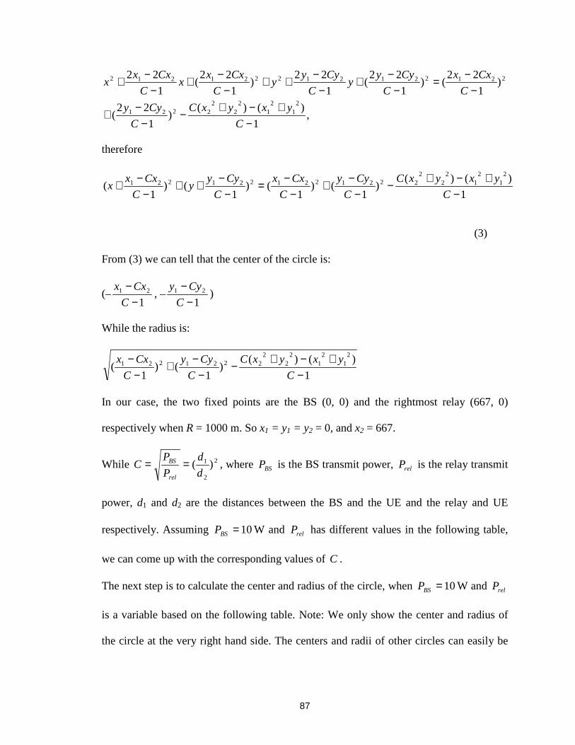
87

,1

)()()

1

22(

)1

22()

1

22(

1

22)

1

22(

1

22

21

21

22

22221

221221212221212

−+−+−

−−+

−−=

−−+

−−++

−−+

−−+

C

yxyxC

C

Cyy

C

Cxx

C

Cyyy

C

Cyyy

C

Cxxx

C

Cxxx

therefore

1

)()()

1()

1()

1()

1(

21

21

22

22221221221221

−+−+−

−−+

−−=

−−++

−−+

C

yxyxC

C

Cyy

C

Cxx

C

Cyyy

C

Cxxx

(3)

From (3) we can tell that the center of the circle is:

(–1

21

−−

C

Cxx, –

121

−−

C

Cyy)

While the radius is:

1

)()()

1()

1(

21

21

22

22221221

−+−+

−−

−+

−−

C

yxyxC

C

Cyy

C

Cxx

In our case, the two fixed points are the BS (0, 0) and the rightmost relay (667, 0)

respectively when R = 1000 m. So x1 = y1 = y2 = 0, and x2 = 667.

While 2

2

1 )(d

d

P

PC

rel

BS == , where BSP is the BS transmit power, relP is the relay transmit

power, d1 and d2 are the distances between the BS and the UE and the relay and UE

respectively. Assuming 10=BSP W and relP has different values in the following table,

we can come up with the corresponding values of C .

The next step is to calculate the center and radius of the circle, when 10=BSP W and relP

is a variable based on the following table. Note: We only show the center and radius of

the circle at the very right hand side. The centers and radii of other circles can easily be

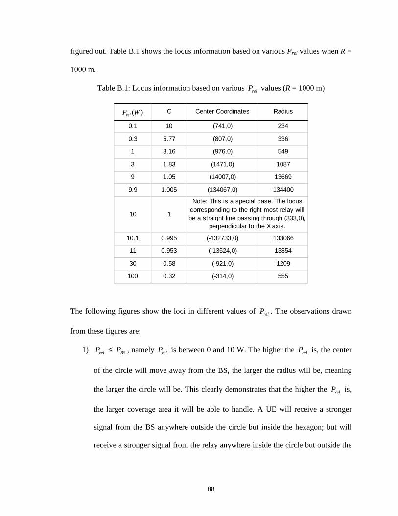
88

figured out. Table B.1 shows the locus information based on various Prel values when R =

1000 m.

Table B.1: Locus information based on various relP values (R = 1000 m)

C Center Coordinates Radius

0.1 10 (741,0) 234

0.3 5.77 (807,0) 336

1 3.16 (976,0) 549

3 1.83 (1471,0) 1087

9 1.05 (14007,0) 13669

9.9 1.005 (134067,0) 134400

10 1

10.1 0.995 (-132733,0) 133066

11 0.953 (-13524,0) 13854

30 0.58 (-921,0) 1209

100 0.32 (-314,0) 555

Note: This is a special case. The locus corresponding to the right most relay will be a straight line passing through (333,0),

perpendicular to the X axis.

)(WPrel

The following figures show the loci in different values of relP . The observations drawn

from these figures are:

1) relP ≤ BSP , namely relP is between 0 and 10 W. The higher the relP is, the center

of the circle will move away from the BS, the larger the radius will be, meaning

the larger the circle will be. This clearly demonstrates that the higher the relP is,

the larger coverage area it will be able to handle. A UE will receive a stronger

signal from the BS anywhere outside the circle but inside the hexagon; but will

receive a stronger signal from the relay anywhere inside the circle but outside the

89

hexagon. It is a special case when relP equals BSP (10 W). The locus is a straight

line perpendicular to the X-axis. As we know, a straight line can be regarded as a

circle with its center infinitely far away from the BS and the radius is an infinite.

2) relP ≥ BSP , namely relP is no less than 10 W. The center of the circle moves to the

other side of the relay creating this circle. The higher the relP is, the center of the

circle will move towards the BS, the smaller the radius will be, meaning the

smaller the circle will be. The coverage responsibility between the BS and the

relay is on the contrary to the above scenario, e.g., a UE will receive a stronger

signal from the BS anywhere inside the circle but outside the hexagon; but will

receive a stronger signal from the relay anywhere outside the circle but inside the

hexagon.

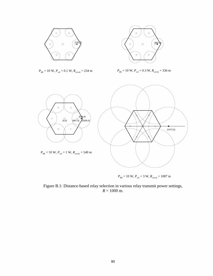
90

(0,0) (667,0) (1000,0)

(976,0)

(741,0) (807,0)

(1471,0)

PBS = 10 W, Prel = 0.1 W, Rcircle = 234 m PBS = 10 W, Prel = 0.3 W, Rcircle = 336 m

PBS = 10 W, Prel = 1 W, Rcircle = 549 m

PBS = 10 W, Prel = 3 W, Rcircle = 1087 m

Figure B.1: Distance-based relay selection in various relay transmit power settings,R = 1000 m.

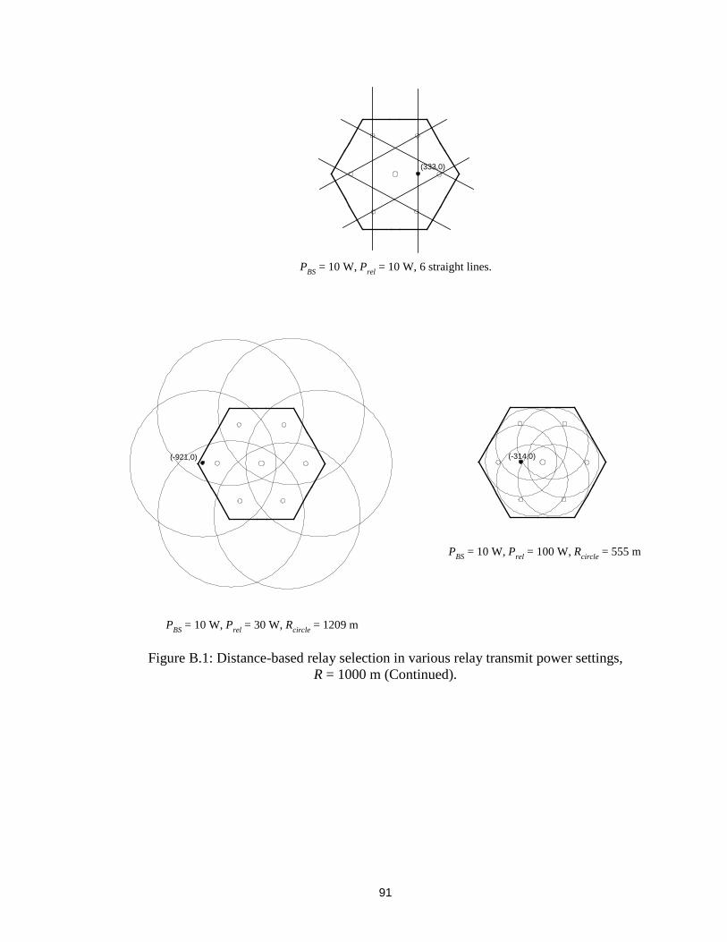
91

(333,0)

(-314,0)(-921,0)

PBS = 10 W, Prel = 30 W, Rcircle = 1209 m

PBS = 10 W, Prel = 100 W, Rcircle = 555 m

PBS = 10 W, Prel = 10 W, 6 straight lines.

Figure B.1: Distance-based relay selection in various relay transmit power settings,R = 1000 m (Continued).

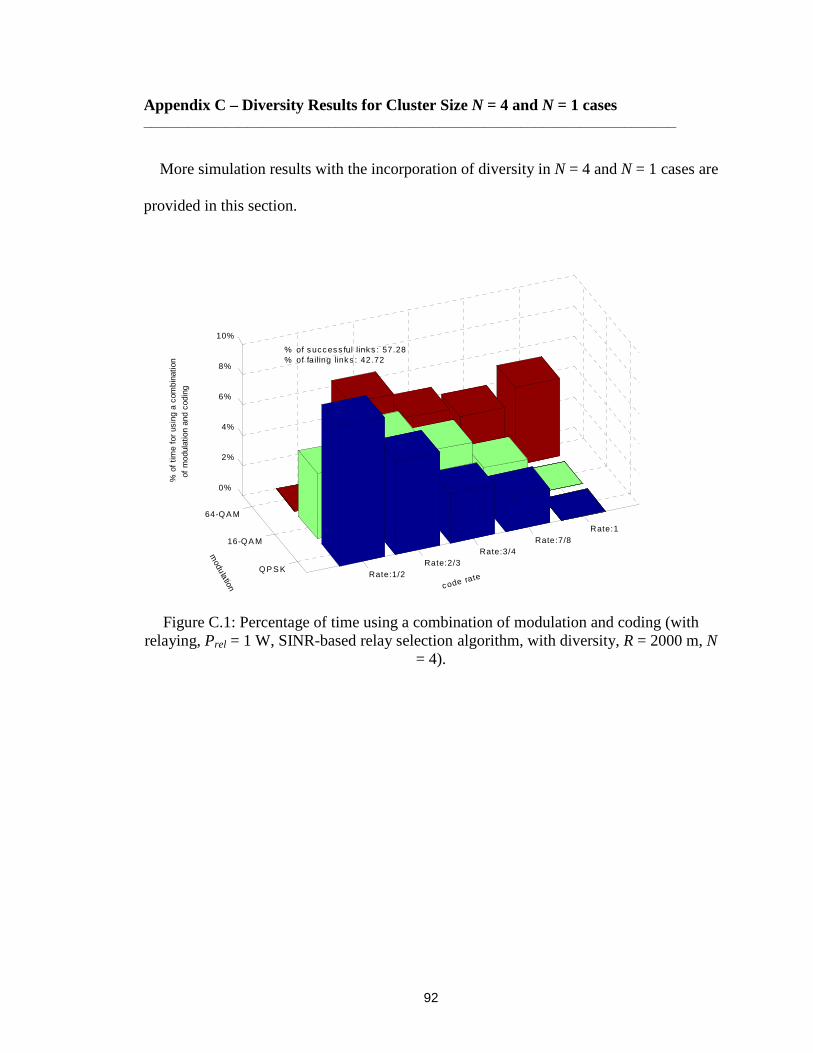
92

Appendix C – Diversity Results for Cluster Size N = 4 and N = 1 cases________________________________________________________________________

More simulation results with the incorporation of diversity in N = 4 and N = 1 cases are

provided in this section.

QP S K

16-QA M

64-QA M

Rate:1/2Rate:2/3

Rate:3/4Rate:7/8

Rate:1

0%

2%

4%

6%

8%

10%

code rate

modulation

% o

f tim

e fo

r us

ing

a co

mbi

natio

n

of m

odul

atio

n an

d co

ding

% of s ucc es s ful link s : 57.28% of failing link s : 42.72

Figure C.1: Percentage of time using a combination of modulation and coding (withrelaying, Prel = 1 W, SINR-based relay selection algorithm, with diversity, R = 2000 m, N

= 4).

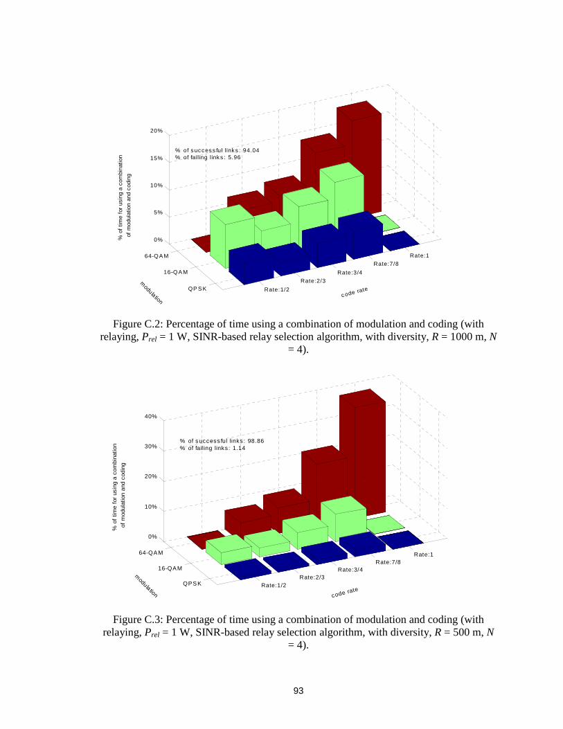
93

QP S K

16-QA M

64-QA M

Rate:1/2

Rate:2/3

Rate:3/4

Rate:7/8

Rate:1

0%

5%

10%

15%

20%

c ode ratem

odulation

% o

f tim

e fo

r us

ing

a co

mbi

natio

n

of m

odul

atio

n an

d co

ding

% of s ucc es s ful link s : 94.04% of failing link s : 5.96

Figure C.2: Percentage of time using a combination of modulation and coding (withrelaying, Prel = 1 W, SINR-based relay selection algorithm, with diversity, R = 1000 m, N

= 4).

QPSK

16-QAM

64-QAM

Rate:1/2Rate:2/3

Rate:3/4Rate:7/8

Rate:1

0%

10%

20%

30%

40%

code rate

modula tion

% o

f tim

e fo

r us

ing

a co

mbi

natio

n of

mod

ulat

ion

and

codi

ng

% of success ful links : 98.86% of failing links : 1.14

Figure C.3: Percentage of time using a combination of modulation and coding (withrelaying, Prel = 1 W, SINR-based relay selection algorithm, with diversity, R = 500 m, N

= 4).

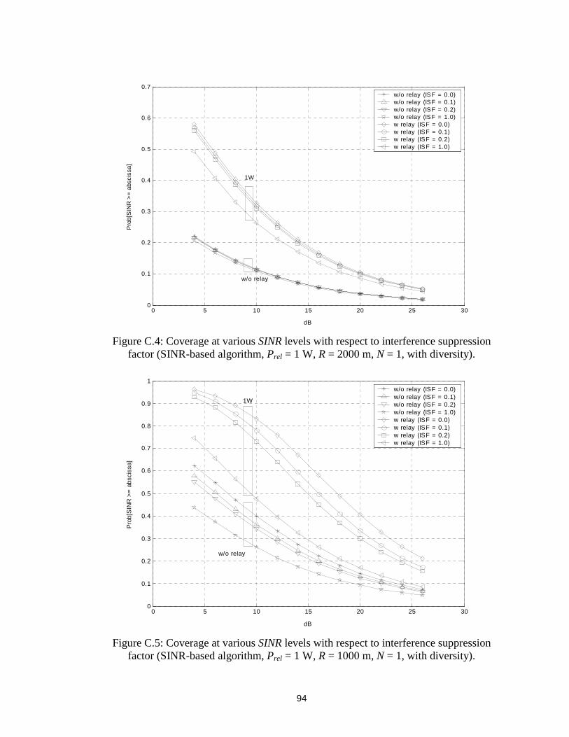
94

0 5 10 15 20 25 300

0.1

0.2

0.3

0.4

0.5

0.6

0.7

dB

Pro

b[S

INR

>=

abs

ciss

a]

w/o relay (ISF = 0.0)w/o relay (ISF = 0.1)w/o relay (ISF = 0.2)w/o relay (ISF = 1.0)w relay (ISF = 0.0)w relay (ISF = 0.1)w relay (ISF = 0.2)w relay (ISF = 1.0)

1W

w/o relay

Figure C.4: Coverage at various SINR levels with respect to interference suppressionfactor (SINR-based algorithm, Prel = 1 W, R = 2000 m, N = 1, with diversity).

0 5 10 15 20 25 300

0.1

0.2

0.3

0.4

0.5

0.6

0.7

0.8

0.9

1

dB

Pro

b[S

INR

>=

abs

ciss

a]

w/o relay (ISF = 0.0)w/o relay (ISF = 0.1)w/o relay (ISF = 0.2)w/o relay (ISF = 1.0)w relay (ISF = 0.0)w relay (ISF = 0.1)w relay (ISF = 0.2)w relay (ISF = 1.0)

1W

w/o relay

Figure C.5: Coverage at various SINR levels with respect to interference suppressionfactor (SINR-based algorithm, Prel = 1 W, R = 1000 m, N = 1, with diversity).

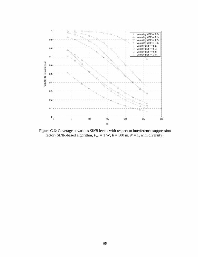
95

0 5 10 15 20 25 300

0.1

0.2

0.3

0.4

0.5

0.6

0.7

0.8

0.9

1

dB

Pro

b[S

INR

>=

abs

ciss

a]

w/o relay (ISF = 0.0)w/o relay (ISF = 0.1)w/o relay (ISF = 0.2)w/o relay (ISF = 1.0)w relay (ISF = 0.0)w relay (ISF = 0.1)w relay (ISF = 0.2)w relay (ISF = 1.0)

Figure C.6: Coverage at various SINR levels with respect to interference suppressionfactor (SINR-based algorithm, Prel = 1 W, R = 500 m, N = 1, with diversity).