performance analysis of cellular networks with

HAL Id: hal-01824986https://hal.inria.fr/hal-01824986v1

Preprint submitted on 27 Jun 2018 (v1), last revised 9 Sep 2019 (v2)

HAL is a multi-disciplinary open accessarchive for the deposit and dissemination of sci-entific research documents, whether they are pub-lished or not. The documents may come fromteaching and research institutions in France orabroad, or from public or private research centers.

L’archive ouverte pluridisciplinaire HAL, estdestinée au dépôt et à la diffusion de documentsscientifiques de niveau recherche, publiés ou non,émanant des établissements d’enseignement et derecherche français ou étrangers, des laboratoirespublics ou privés.

Performance analysis of cellular networks withopportunistic scheduling using queueing theory and

stochastic geometryBartlomiej Blaszczyszyn, Mohamed Kadhem Karray

To cite this version:Bartlomiej Blaszczyszyn, Mohamed Kadhem Karray. Performance analysis of cellular networks withopportunistic scheduling using queueing theory and stochastic geometry. 2018. �hal-01824986v1�

https://hal.inria.fr/hal-01824986v1

https://hal.archives-ouvertes.fr

1

Performance analysis of cellular networks withopportunistic scheduling using queueing theory and

stochastic geometryBartłomiej Błaszczyszyn∗ and Mohamed Kadhem Karray†

Abstract—Combining stochastic geometric approach with someclassical results from queuing theory, in this paper we proposea comprehensive framework for the performance study of largecellular networks featuring opportunistic scheduling. Rapid andverifiable with respect to real data, our approach is particu-larly useful for network dimensioning and long term economicplanning. It is based on a detailed network model combining aninformation-theoretic representation of the link layer, a queuing-theoretic representation of the users’ scheduler, and a stochastic-geometric representation of the signal propagation and thenetwork cells. It allows one to evaluate principal characteristicsof the individual cells, such as loads (defined as the fraction oftime the cell is not empty), the mean number of served users inthe steady state, and the user throughput. A simplified Gaussianapproximate model is also proposed to facilitate study of thespatial distribution of these metrics across the network. Theanalysis of both models requires only simulations of the pointprocess of base stations and the shadowing field to estimatethe expectations of some stochastic-geometric functionals notadmitting explicit expressions. A key observation of our ap-proach, bridging spatial and temporal analysis, relates the SINRdistribution of the typical user to the load of the typical cell ofthe network. The former is a static characteristic of the networkrelated to its spectral efficiency while the latter characterizes theperformance of the (generalized) processor sharing queue servingthe dynamic population of users of this cell.

Index Terms—user-throuhgput, traffic demand, cell-load equa-tions, cellular network, opportunistic scheduling, typical cell,queueing theory, point process, ergodicity, Palm theory, Little’slaw, measurements

I. INTRODUCTION

Motivated by the increasing traffic in commercial cellularnetworks featuring opportunistic scheduling policies, in thispaper we propose a mathematical model, based on queueingtheory and stochastic geometry, allowing one to evaluateperformance of such networks, with a particular focus on thevariability of the quality of service characteristics across thenetwork. We build on our previous work [1], where a networkevaluation model has been proposed, assuming a homogeneousspace-time Poisson process of call arrivals served by a spatiallystationary cellular network, with processor sharing queuemodels operating at all network stations. These queues are

∗INRIA-ENS, 2 rue Simone Iff 75589 Paris, France Email:[email protected]†Orange Labs; 44 Avenue de la Republique, 92320 Chatillon, France

Email: [email protected] paper reports the results of a research undertaken under the contract

CRE No G10192 between Inria and Orange.

related to each other via some system of cell-load equations tocapture the dependence caused by the extra-cell interference.

In this paper we assume generalized processor sharingqueues allowing one to model a large class of opportunisticschedulers and we evaluate their impact on the steady stateuser and cell performance metrics. Among principal metricsstudied via the cell-load equations are cell loads (defined as thefraction of time the station is busy), mean number of users andtheir throughput at individual network cells. Following [2], wealso propose an efficient Gaussian approximate model for therapid study of the spatial distribution of these metrics acrossthe network.

Stochastic-geometric analysis of the cell-load equationsreveals a key observation relating the SINR distribution ofthe typical user in the network to the load of the typical cellof the network. This relation, captured by what we call typicaluser–cell exchange formula, is a consequence of the inverseformula of Palm calculus, which itself is a special case of avery general conservation law observed in stationary systems,known as mass transport principle. (This general law subsumesmany classical results in stochastic geometry and queueingtheory, for example the famous Little’s law.)

The SINR distribution at the typical location characterizespotential performance of the network related to its spectralefficiency. It is often studied in stochastic geometric mod-els of cellular networks. On the other hand, the cell loadcharacterizes the performance of the (generalized) processorsharing queue serving the dynamic population of users. Thus,the aforementioned user-cell exchange formula is a bridgebetween the stochastic-geometric analysis of the network andthe queueing theoretic study of the user service.

Our models are studied in a semi-analytic way involvingonly simulations of the point process of base stations and theshadowing field to estimate the expectations of some stochasticgeometric functionals not admitting explicit expressions. Alllower level performance characteristics, involving the linklayer and the opportunistic scheduler admit explicit expres-sions and need not be estimated by simulations. This approachallows one for a rapid and verifiable with respect to real dataevaluation of the impact of the opportunistic scheduling onthe global network performance. It is particularly useful fornetwork dimensioning and long term economic planning.

A. Paper organizationThe remaining part of the paper is organized as follows.

We complete our introduction by discussing in Section I-B

2

some related work. The fundamental model is described inSection II. Theoretical analysis of this model and a Gaussianapproximate model is presented in Section III. Our numericalstudy, including validation of the Gaussian model with respectto the fundamental model and with respect to real data is pre-sented in Section IV. We recapitulate our work in Section V.

B. Related work

A large amount of literature has emerged on the perfor-mance analysis of cellular networks; a complete review fallsout of the reach of this paper. In what follows we mentiononly some works that we found most relevant.

a) Pure simulation approach: Many network operatorsand other actors develop complex and time consuming simu-lation tools such as those developed by the industrial contribu-tors to 3GPP (3rd Generation Partnership Project) [3]. Thereare many other simulation tools such as TelematicsLab LTE-Sim [4], University of Vien LTE simulator [5, 6] and LENAtool [7, 8] of CTTC, which are not necessarily compliantwith 3GPP. Our approach requires only static simulations toestimate some stochastic geometric expectations with all lowerlevel performance characteristics admitting explicit expres-sions. This makes it significantly more rapid.

b) Analytic approach: Most of the analytic studies ofthe performance of cellular networks focus on some particularlayer. For example, information theoretic characterization ofthe individual link performance is proposed in [9–11]. Queuingtheoretic modeling and analysis of the user traffic can be founde.g. in [12–17]. Following the pioneer work in [18] and [19],a large amount of literature uses stochastic geometry to buildexplicit expressions of the distribution of the downlink SINRat a typical location in the network; see [20, Chapters 5–7]for a complete treatment of this subject. Our comprehensiveapproach to the evaluation of large cellular networks stronglybuilds on these more focused studies.

c) Space-time models: While all modern stochastic ge-ometric models of cellular networks integrate expressionsinspired by information theory, using queueing theory inrandom geometric context is more rare and thus deserves afew comments.

Theoretical foundations of spatial Markovian queueing sys-tems have been worked out in [21]. Among early works usingthis setting, in [22] blocking probabilities of the constant bit-rate traffic were studied via a spatial Erlang loss formula.In [23] some decentralized congestion control schemes werestudied in the context of data traffic using spatial processorsharing queues. Both papers assume spatial Markovian arrivalsto some subset of the plane representing one cell of thenetwork. Full interference from other base stations is taken intoaccount without capturing the interaction between networkcells. To the best of our knowledge, this latter idea appearsfor the fist time in [24], and independently, in the contextof a hexagonal network model in [17]. However, no spatialstochastic geometric analysis of these equations and of thenetwork is proposed there.

More recently and in a different context, [25] leveragesstochastic geometric and queueing theoretic techniques to

investigate the performance of some cooperative communica-tions in decentralized wireless networks. In [26] the uplinkof K-tier heterogeneous networks is studied using M/G/1queueing model in stochastic geometric setting. Delays in theheterogeneous cellular networks with spatio-temporal randomarrival of traffic are studied in [27]. The authors of [28]investigate interference, queueing delay and network through-put in interference-limited networks while taking into accountdiverse QoS requirements. These theoretical works have notyet been compared to real data.

Our study features in particular realistic evaluation of theopportunistic scheduler and the spatial variability of the qualityof service across the networks. In what follows we commenton some previous work in this matter.

d) Opportunistic schedulling: It leverages an inherentdiversity of wireless networks provided by independently time-varying channels across the different users. The benefit ofthis diversity is exploited by scheduling transmissions to userswhen their instantaneous channel quality is near its best values.The diversity gain increases with the dynamic range of thefluctuations; it can be improved by some dynamic beamform-ing [29] in environments with little scattering and/or slowfading. Specific opportunistic schedulers for wireless systemshave been proposed and studied for some thirty years. Thereis a large number of papers available that propose differentopportunistic scheduling techniques. These range from simpleheuristic algorithms to complex mathematical models; see asurvey article [30] published in 2013. The aims of thesetechniques vary; some proposals are only designed to increasethe total network capacity, while others seek to enhance QoSobjectives such as throughput and fairness.

In terms of real world implementations, opportunistic sched-ulers started only appearing from the 3.5G (HSDPA) net-work technology. The current 4G technology leverages someopportunistic scheduling techniques to propose higher userrates. Although it is not always possible to know the precisenature of the implemented schemes, as we shall see in thispaper, some aspects of this performance can be capturedat the level of individual network cells by using relativelysimple mathematical models of generalized processor sharingqueues [12] with an appropriate scheduling gain function.

The authors of [31] evaluate some opportunistic schedulers,both numerically and analytically, under several fading distri-butions and bandwidth constraints. An ubiquitous assumptionis that the scheduler is not aware of the interference. Thisreduces the scheduling gain as recently shown in [32] assum-ing Voronoi network model and in [33] for the bipolar networkmodel. These studies concentrate on the user peak bit-rate anddo not evaluate user throughput that depends on the networkload.

e) Spatial distribution of the quality of service: Userquality of service (e.g. throughput) and network performancemetrics (e.g. cell loads) represent some mean characteristicsevaluated locally in the network (e.g. for each cell) oversome relatively short time intervals (usually one hour). Fora given time interval, these characteristics can significantlyvary across the cells, even if the user traffic can be consideredas spatially homogeneous. This phenomenon, observed in data

3

systematically collected by mobile operators [34–36] is relatedto the fact that real networks are not regular (hexagonal) butexhibit non-negligible variability of the size and geometry ofcells, resulting form base station deployment constraints andhaphazard propagation (shadowing) effects.

In stochastic-geometric models the aforementioned irregu-larity of the network is represented by appropriate point pro-cess (usually Poisson) representing locations of base stationsand random shadowing field (often assumed log-normal). Inthis approach, the spatial distribution of performance metricscorresponds to the conditional expectations of the correspond-ing functions given a realization of the point process ofbase stations and a realization of the shadowing field. Theseexpectations represent averaging over fast fading and dynamicconfigurations of users. The term “meta-distribution” wascoined in [37] for the conditional distribution of the SINRgiven location of stations; see [20, Section 6.3] for moredetails.

Attention to the these conditional expectations has beendrown in [38] by showing that the spatial averaging of somelocally finite network characteristics — mean local delaysin the Poisson bipolar network model in the cited paper —can lead to infinite spatial averages in several practical cases,including the Rayleigh fading and positive thermal noise case.This mathematical fact says that a relatively large fraction ofusers experience in this network model large (but finite) localdelays.

The spatial variability of the performance metrics was alsoconsidered in the studies of load balancing between cells. Forexample, [39] proposes an algorithm that compensates thespatial disparity of traffic demand, while [40] and [41] focuson the improvement of the performance of heterogeneous net-works by elaborating different algorithms that insure energy,spectrum and load balancing.

f) Our previous work: The current approach based onthe stochastic geometric study of the cell load equations wasinitially proposed in [1]. It has been extended allowing one totake into account heterogeneous networks (micro-macro cells)in [42] and spatial non-homogeneity in [43]. The study of thespatial distribution of the quality of service was initiated usingthis approach in [44]. The Gaussian approximated model wasproposed in [2]. In all these works one assumes round-robinscheduler.

II. DETAILED MODEL DESCRIPTION

We shall now describe our space-time network model.

A. Network architecture

We describe first all static elements of the network model;they do not evolve in time.

1) Locations and transmission powers of base stations:We consider locations {X1, X2, . . .} of base stations (BS)on the plane R2 as a realization of a point process, whichwe denote by Φ.1 We denote by P the probability on some

1According to the formalism of the theory of point processes (cf e.g. [45]),a point process is a random measure Φ =

∑n δXn , where δx denotes the

Dirac measure at x.

probability space on which Φ and all other random variablesconsidered in what follows are defined and assume that underP, Φ is stationary and ergodic 2 with positive, finite intensityλ (mean number of BS per unit of surface). We denote byPn (Pn ≥ 0 ) the power emitted by BS Xn and assume thatPn’s are independent, identically distributed (i.i.d.) marks ofthe process Φ.

2) Propagation effects: The propagation loss is modeledby a deterministic path-loss function l(x) = (K |x|)β , whereK > 0 and β > 2 are given constants, and some randompropagation effects. We split these effects into two categoriesconventionally called (fast) fading and shadowing. The formerwill be taken into account in the model at the link-layer,specifically in the peak bit-rate function, cf. Example 1. Theshadowing impacts the choice of the serving BS and thus needsto be considered together with the network geometry. To thisregard, we assume that the shadowing between a given stationXn ∈ Φ and all locations y in the plane is modeled by somepositive valued stochastic process Sn(y − Xn). We assumethat the processes Sn(·) are i.i.d. marks of Φ, independentof the transmission powers Pn. Moreover we assume thatS1(y) are identically distributed across y, but do not makeany assumption regarding the dependence of Sn(y) across y.We denote by Φ the point process of base station locations Φwith its (independent) marks described above.

The inverse of the power received at y from BS Xn,averaged over fast fading, denoted by LXn(y) is given by

LXn(y) :=l(|y −Xn|)

PnSn(y −Xn). (1)

Slightly abusing the terminology, we will call LXn(·) thepropagation-loss process from station Xn. Sometimes we willsimplify the notation writing LX(·) for the propagation-lossof BS X ∈ Φ and PX for its transmission power.

3) Service zones, SINR and peak bit-rates: We assume thateach (potential) user located at y on the plane is served by theBS offering the strongest received power among all the BS inthe network. Thus, the zone served by BS X ∈ Φ, denotedby V (X), which is traditionally called the cell of X (even ifrandom shadowing makes it need not to be a polygon or evena connected set) is given by

V (X) ={y ∈ R2 : LX(y) ≤ LY (y) for allY ∈ Φ

}. (2)

We define the (downlink) SINR at location y ∈ V (X) (withrespect to the serving BS X ∈ Φ)

SINR(y, Φ) :=1/LX(y)

N +∑Y ∈Φ\{X} ϕY /LY (y)

, (3)

where N is the noise power and ϕY ∈ [0, 1] are some activityfactors related to BS Y ∈ Φ, which will be specified inSection II-C2. Note, they weight in (3) the transmission powersin the interference term of the SINR to account for the factthat these BS might not transmit with their respective maximalpowers PY . In general, we assume that ϕY are additional (not

2Stationarity means that the distribution of the process is translationinvariant, while ergodicity allows to interpret some mathematical expectationsas spatial averages of some network characteristics.

4

necessarily independent) marks of the point process Φ. In fact,we shall specify ϕY in Section II-C2 as some functionalsof the locations of all points and other marks of the pointprocess Φ.

We assume that the peak bit-rate at location y, definedas the maximal download bit-rate available at location y(achievable when all resources of the station serving thislocation are devoted to a single user located at y) is somefunction R(SINR) of the SINR = SINR(y, Φ) at this location.Our general analysis presented in this paper does not dependon any particular form of this function. For example, one mightexpress R(·) in relation to the information theoretic capacityof some channel model.

Example 1 (AWGN MIMO channel): The theoretical capac-ity of the additive white Gaussian noise (AWGN) multiple-input-multiple-output (MIMO) channel is given by the formula(cf. [46, Theorem 1]).

RMIMO(ξ) = WE[log2 det(I +ξ

tHH∗)] (4)

where the expectation E [·] is with respect to the circularly-symmetric complex Gaussian matrix H (corresponding toRayleigh fading) with the number of lines r and columns tcorresponding to the number of receiving and transmittingantennas, respectively, with H∗ being its complex conjugate;ξ is the SNR par transmitting antenna, W is the frequencybandwidth and I is the appropriate identity matrix. Interpretingthe extra-channel interference as a part of the noise and takingξ for the SINR makes the expression in (4) lower bounds theaforementioned MIMO channel capacity; [11].

4) Scheduling gain: We consider variable bit-rate (VBR)traffic; i.e., users arrive to the network (in a way to bedescribed in Section II-B1) and request transmissions of somedata volumes at bit-rates decided by the network. When severalusers are present in a cell, they need to share the serving BSresources, which means that in general they do not receivetheir full peak bit-rates. In this paper we assume that whenn users are present in the cell then each of them receivesa fraction g(n)/n of its own peak bit-rate, i.e., the servicerate R(SINR)g(n)/n. Such a service discipline is calledgeneralized processor sharing with scheduling gain g(n). Ageneral assumption required for the ergodicity and stability ofthe processor sharing queue, cf. Section II-C1, is g(n) > 0for n ≥ 1.

Example 2 (Round robin system): In this case g(n) ≡ 1.This is the usual processor sharing assumption.If g(n) > 1 then the service rates of all users are higherthan in the round robin case. This is a natural assumption inthe context of this paper, where higher service rates arise asa consequence of an opportunistic scheduling of the packettransmissions to different users. This also explains why wecall g(·) the scheduling gain.3

3 If one wants to preserve the interpretation of the peak bit-rate R(SINR)as the maximal rate, available when one user is served, then g(n) ≤ n withg(1) = 1.

Example 3 (Opportunistic channel scheduling): The follow-ing function was proposed in [12] to model the performance ofsome opportunistic channel scheduling for cellular networks

g(n) = 1 + 1/2 + . . .+ 1/n, n ≥ 1. (5)

It corresponds to the case of independent, time-varyingRayleigh fading and user transmissions scheduled at timeswhen they observe their best channel conditions. Note that inthis case the scheduling gain g(n) increases to infinity with n.

Example 4 (Truncated opportunistic channel scheduling):In practice, the scheduler gain is limited and the followingvariant of (5) is of interest

g(n) =

{1 + 1/2 + . . .+ 1/n for 1 ≤ n ≤ nmax

g(nmax) for n > nmax.(6)

B. Users and service policy

We describe now the space-time process of user arrivals(and departures).

1) Traffic demand: As we already mentioned, we considerthe VBR traffic: users arrive and request transitions of somedata volumes. (The transmission rates vary in space and intime, depending on the user locations and the number of usersserved by the station at a given time; cf. Section II-A4.) Morespecifically, we assume a homogeneous time-space Poissonpoint process of user arrivals of intensity γ arrivals persecond per km2. This means that the time between twosuccessive arrivals in a given zone of surface S is exponentiallydistributed with parameter γ×S, and all users arriving to thiszone take their locations independently and uniformly. Thetime-space process of user arrivals is independently markedby random, identically distributed volumes of data the userswant to download from their respective serving BS. Thesevolumes are arbitrarily distributed and have mean 1/µ bits.Finally, we assume that the time-space point process of userarrivals marked by the data volumes is independent of thespatial, marked point process Φ of base stations.

The above arrival process induces the traffic demand persurface unit ρ = γ/µ expressed in bits per second per km2.Given Φ, the traffic demand in the cell of any BS X ∈ Φequals

ρ(X) = ρ |V (X)| , (7)

where |A| denotes the surface of the set A; ρ(X) is expressedin bits per second.

2) Processor sharing systems: Given Φ, the evolution ofthe number of users present in any given cell follows the(generalized) spatial, multi-class processor queue model. Thatis, users start being served (downloading their volumes of data)immediately after their arrivals to cells. Their transmissionrates depend on their SINR conditions and the number of userspresent in the same cell as described in Section II-A4. Usersleave the system immediately after having downloaded theirvolumes. Note that given a realization of the point process Φ ofbase stations and its marks, the stochastic processes describingthe evolution of different cells are independent.

5

C. Generalized processor sharing queues

Let us first recall some basic results regarding the steadystate characteristics of the processor sharing queues describingthe temporal evolution of the service in any given cell of thenetwork. Then, we shall introduce a key concept of this paperthat is cell load equations, allowing one to capture the spatialdependence of service processes in different cells.

1) Free cell performance characteristics: Given Φ, for allX ∈ Φ, denote by ρc(X) the harmonic mean of the peakbit-rate over the cell V (X)

ρc(X) :=|V (X)|∫

V (X)R−1(SINR(y, Φ))dy

, (8)

where R−1(. . . ) = 1/R(. . . ). We will call ρc(X) the criticaltraffic demand of cell X . Together with the cell load ρ(X)defined in (7) and the scheduling gain function g(·) it allowsone to characterize the stability of the generalized processorsharing queue and express important mean characteristics ofits steady state, and even characterize its distribution; [47, 48].Indeed, the processor sharing queue of cell V (X) is stable ifand only if its traffic demand ρ(X) is smaller than the criticaltraffic demand times the asymptotic scheduling gain 4

ρ(X) < ρc(X)× limn→∞

g(n). (9)

The probability that the cell is idle (has no users) at thesteady state, denoted by I(X), is given by

I(X) =( ∞∑n=0

(ρ(X)/ρc(X))n

G(n)

)−1

, (10)

where G(0) := 1 and for n ≥ 1, G(n) := g(1) . . . g(n). Thecomplement of this probability, the cell busy probability, willbe called in what follows the cell load of X and denoted byθ(X)

θ(X) := 1− I(X) . (11)

Note that the cell is stable (condition (9) is satisfied) if I(X) >0 or, equivalently, the cell load θ(X) < 1 and unstable ifθ(X) > 1.

The mean number of users N(X) in the steady state of thecell V (X) is given by

N(X) = I(X)

∞∑n=1

n(ρ(X)/ρc(X))n

G(n), (12)

provided the cell is stable and N(X) =∞ otherwise. Finally,the mean user throughput r(X) in cell V (X) is defined as theratio of the mean data volume to the mean typical user servicetime. Using the Little’s law, one can show that

r(X) =ρ(X)

N(X). (13)

Example 5 (Round robin scheduling): In case g(n) ≡ 1, cf.Example 2, the cell is stable if ρ(X) < ρc(X). Under thiscondition θ(X) = ρ(X)/ρc(X), N(X) = θ(X)/(1 − θ(X))and r(X) = ρc(X)− ρ(X).

4We assume that g(n) > 0 for all n ≥ 1 and that limit in (9) exists andis strictly positive. If the limit does not exist the condition is more involved.

Example 6 (Opportunistic scheduling): Applying thescheduling gain from Example 3 makes cells stable for allvalues of the traffic demand ρ(X) < ∞. The correspondingexpressions for θ(X), N(X) and r(X) are less explicit, butare still amenable to numerical calculations.

2) Cell load equations and spatially correlated cells:The individual cell characteristics described in the previoussection depend on the location of all base stations, shadowingrealizations but also on the cell activity factors ϕY , Y ∈ Φ,introduced in Section II-A3 to account for the fact that BSmight not transmit with their respective maximal powers PY .

It would be quite natural to assume that a given BS transmitswith its maximal power PY when it serves at least one userand does not transmit otherwise 5. Taking this fact into accountin an exact way would require defining ϕY as the indicatorsthat Y ∈ Φ is busy, thus making ϕY dependent not only onΦ but also on the varying in time process of users. This, inconsequence, would lead to the probabilistic dependence of theservice processes at different cells, thus revoking the explicitexpressions for their characteristics presented in Section II-Cand, in fact, making the model analytically non-tractable. 6

To avoid this difficulty we take into account the activityof station Y in a simpler way, multiplying its maximaltransmitted power by the probability θ(X) that it is busy (thatis serves at least one user) in the steady state. In other words,in the SINR expression (3) we take ϕY = θ(Y ) where θ(Y )is the load of the cell Y ; i.e.,

SINR(y, Φ) =1/LX(y)

N +∑Y ∈Φ\{X} θ(Y )/LY (y)

. (14)

Making the above assumption, we preserve the independenceof the queueing processes at all cells V (X), X ∈ Φ, given therealization Φ of the process of BS with their shadowing andpower marks. We call this simplifying assumption the time-decoupling of the cell processes. Note that the cell processesremain coupled in space. By this we mean two observations:Firstly, as in Section II-C1, ρ(X) and ρc(X) depend onthe realization of the process Φ, in particular on the servicezones V (X) which are dependent sets. However, additionally,the critical traffic demands ρc(X) of all stations X ∈ Φ(and in consequence all other time-stationary characteristicsof the queueing processes) cannot be any longer calculatedindependently for all cells via (8), given Φ, but are solutionsof the following fixed point problem, which we call cell loadequations: for all X ∈ Φ

ρc(X) =|V (X)|∫

V (X)

R−1(

1/LX(y)N+

∑Y∈Φ\{X} θ(Y )/LY (y)

)dy

, (15)

where θ(Y ) depends on ρc(Y ) and the traffic demand ρ(X)via (11) and (10). This system of equations introducesadditional spatial dependence between mean performancecharacteristics of different cells. It needs to be solved for

5Analysis of more sophisticated power control schemes is beyond the scopeof this paper.

6We are not aware of any result regarding the stability and performance ofsuch a family of dependent queues.

6

{ρc(X)}X∈Φ (equivalently for {θ(X)}X∈Φ) given Φ, i.e., net-work, power and shadowing realization. Other characteristicsof each cell are then deduced from the cell load and trafficdemand using the relations described in Section II-C, involvingthe scheduling gain function g(·).

We repeat, cell load equations (15) capture spatial depen-dence between the processor sharing queues of different cells,while allowing for their temporal independence, given thenetwork realization.

Remark 1: [Network spatial stability] A natural questionarises regarding the existence and uniqueness of the solutionof the equations (15). Note that the mapping in the right-hand-side of (15) is increasing in all θ(Y ), Y ∈ Φ provided thefunction R is increasing. Using this property it is easy tosee that successive iterations of this mapping started eitherfrom θ(Y ) = 0 for all Y ∈ Φ or from θ(Y ) = 1 for allY ∈ Φ, converge to a minimal and maximal solution of (15),respectively. An interesting theoretical question regards theuniqueness of the solution of (15), in particular for a random,say Poisson, point process Φ. Answering this question, whichwe call spatial stability of the model, is beyond the scopeof this paper. Existence and uniqueness of the solution of avery similar problem (with finite number of stations and adiscrete traffic demand) is proved in [24]. In the remainingpart of the paper, to fix the attention, by the solution of (15)we understand the minimal one.

3) Equivalent form of cell load equations: In view of thefuture analysis, it is customary to consider for each station Xthe ratio of the traffic demand to the critical traffic demand

ρ′(X) :=ρ(X)

ρc(X). (16)

We call ρ′(X) the normalized traffic demand. Note by (7)and (8)

ρ′(X) = ρ

∫V (X)

R−1(SINR(y, Φ))dy . (17)

All characteristics considered in Section II-C, including thestability condition, can be expressed in terms of the vector(ρ(X), ρ′(X)), with the following equivalent form of the cellload equations (15) with unknown vector {ρ′(X)}X∈Φ:

ρ′(X) = ρ

∫V (X)

R−1

(1/LX(y)

N +∑Y ∈Φ\{X} θ(Y )/LY (y)

)dy ,

(18)

where

θ(Y ) = 1−( ∞∑n=0

(ρ′(Y ))n

G(n)

)−1

, (19)

with G(·) as in (10).

III. SPATIAL NETWORK PERFORMANCE ANALYSIS

Individual cell characteristics considered in Section II-Care important performance indicators of the service evaluatedfor each BS X of the network. Mathematically, they formsome non-independent marks of the points X ∈ Φ, which aredeterministic functions of Φ modeling locations of BS, their

powers and the shadowing fields. If a given realization of theprocess Φ were an exact representation of some network, thenthe above characteristics would provide the QoS metrics inthe respective cells. However, the point process Φ is usuallymerely a probabilistic model of the base station placement, andconsequently a given point X ∈ Φ and its cell characteristicsdo not correspond to any really existing BS. Nevertheless, thewhole family of cell characteristics, parametrized by X ∈ Φ,does carry some information about the spatial distribution ofthe network performance characteristics. Consequently, whendoing some appropriate averaging over the individual cellcharacteristics one can capture the global network performancelaws. In what follows we propose two approaches in thisregard, a detailed typical cell analysis and a simplified meancell analysis.

A. The detailed model and its typical cell analysis

By the detailed model we understand the point processΦ with its individual cell characteristics considered in Sec-tion II-C as dependent marks. These marks are fully charac-terized by the two-dimensional mark (ρ(X), ρ′(X)), wherethe normalized traffic demands ρ′(X), X ∈ Φ solve the(equivalent) cell load equations (18), cf. Section II-C3.

1) The typical cell of the detailed model: We are interestedin the distribution of the vector (ρ(0), ρ′(0)) of the trafficdemand and the modified traffic demand of the typical station7

X0 = 0 under the Palm distribution P0 of the stationaryprocess Φ. All individual cell characteristics of this typicalstation, considered in Section II-C, are deterministic functionsof the vector (ρ(0), ρ′(0)),

Unfortunately, only the expected values E0[ρ(0)] andE0[ρ′(0)] admit explicit expressions. Also, we have somevariance results. These are key elements of some simplifiedanalysis proposed in Section III-B.

2) Mean values: The vector (ρ(0), ρ′(0)) admits the fol-lowing expressions regarding its (Palm) expectation.

Fact 2: We have

E0[ρ(0)] =ρ

λBS, (20)

E0[ρ′(0)] = ρE[1/R(SINR(0, Φ))] . (21)

The result (21) remains true for any stationary (translationinvariant) assumption regarding the marks being the cellactivity factors ϕY , including the particular case ϕY = θ(Y )being the solution of the cell load equations.

Proof: The first equation is quite intuitive: the averagecell surface is equal to the inverse of the average number ofBS per unit of surface. Formally, both equations follow fromthe “inverse formula of Palm calculus” [49, Theorem 4.2.1];see also “typical location-station exchange formula” in [20,Theorem 4.1.4]. In particular, for (21) one uses (18) inconjunction with the inverse formula.

7The typical cell of a stationary network is a mathematical formalizationof a cell whose BS is “arbitrarily chosen” from the set of all stations, withoutany bias towards its characteristics. The formalization is made on the groundof Palm theory, where the typical cell V (0) is this of the BS X0 = 0 locatedat the origin under the Palm probability P0 associated to point process Φ andits stationary probability P.

7

Remark 3: Note that the expectation in the right-hand-sideof (21) is taken with respect to the stationary distribution ofthe BS process Φ. It corresponds to the spatial average of theinverse of the peak bit-rate calculated throughout the network.The only random variable in this expression is the SINRexperienced at an arbitrary location (chosen to be the origin 0)with respect to the base station serving this location (we denotethis station X∗ in (23)) under the stationary distribution of thenetwork Φ. Due to the independence assumption of the processof user arrivals and Φ, it is possible to identify this arbitrarylocation with the location of the typical user. Thus (21) canbe called typical user–cell exchange formula.

Remark 4 (SINR distribution of the typical user): Thedistribution of SINR(0, Φ) is usually estimated in operationalnetworks from user measurements. It also admits some analyt-ical expressions for some particular point processes, in case ofconstant cell activity factors ϕY (without considering cell-loadequations). The most studied is Poisson network model, whereby the Slivnyak’s theorem, the Palm distribution correspondssimply to adding one point X0 = 0 at the origin. In the caseof i.i.d. marked Poisson process, as in our case, this extrapoint gets an independent copy of the mark, with the originalmark distribution. The distribution of the SINR at the typicallocation SINR(0, Φ) in Poisson network model admits someexplicit expressions; cf. [50–52]. Some expressions are alsoavailable for more regular than Poisson network models basedon Ginibre and related determinantal point processes, cf. [53–55]. For a complete treatment of the SINR distribution of thetypical user, see [20, Chapters 5–7].

3) Variance analysis:Fact 5: The square relative standard deviations (SRSD)

Var(ρ(0))

(E0[ρ(0)])2

of the traffic demand in the typical cell model is a scale freefunctional of the network process Φ: it does not depend on theuser traffic and is invariant to any homothetic transformationof the network process.This result is known for the Voronoi cells and was generalizedto the service zones in the model with the shadowing in [2].

We were not able to prove similar result in full generality forthe SRSD of the modified traffic demand ρ′(0) in the typicalcell. However, the following empirical observation was madeand supported by numerical arguments in [2].

Observation 6: The SRSD of the modified traffic demandand the logarithmic correlation coefficient of the typical cellunder Palm probability P0 of Φ

Var(ρ′(0))

(E0[ρ′(0)])2,

Cov(ln ρ(0), ln ρc(0))√Var(ln ρ(0))Var(ln ρc(0))

do not depend significantly on ρ (the traffic demand persurface unit).

4) Ergodic averaging in the detailed model: In order toevaluate further distributional characteristics of the randomvector (ρ(0), ρ′(0)) one needs to approximate them by thespatial (empirical) averages of the vector (ρ(X), ρ′(X)) forX ∈ Φ considered (simulated) in a large enough window,

leveraging the ergodicity of the point process Φ. 8 Thefollowing classical ergodic result is crucial in this regard.

Fact 7: Consider an increasing network window A, say adisc (or square) centered at the origin and the radius (or side)increasing to infinity. If Φ is ergodic then

P0{ρ(0) ≤ u, ρ′(0) ≤ t} (22)

= lim|A|↗∞

1/Φ(A)∑X∈A

1(ρ(X) ≤ u, ρ′(X) ≤ t).

The convergence is P almost sure.The result follows from the ergodic theorem for point pro-cesses (see [49, Theorem 4.2.1], [45, Theorem 13.4.III]).9

The following distributional characteristics of the typicalcell are of particular interest for us and can be obtained usingapproximations (22).• The mean traffic demand E0[ρ(0)].• The mean cell load E0[θ(0)] and the probability distri-

bution function P0{θ(0) ≤ u}. The former gives theaverage load of the network, while the later gives thefraction of cells with load below some value u < 1considered as a critical one.10

• The mean E0[N(0)] and the median m of the number ofusers (defined by P0{N(0) ≤ m} = 1/2) in the typicalcell. The median is more appropriate for networks withlarge disparity of cell sizes, where a few heavily loadedcells can significantly bias the mean E0[N(0)].11

• The mean user throughput E0[r(0)] = E0[ρ(0)/N(0)].Note this is a double averaging: ρ(0)/N(0) correspondsto the time-average user throughput in the typical celland the palm expectation E0 corresponds to the spatialaverage of this quantity over the network cells. Note, ingeneral E0[r(0)] 6= E0[ρ(0)]/E0[N(0)].12

B. Extended mean cell model

The expectations given in Fact 2 do not give enough infor-mation regarding the distribution of the vector (ρ(0), ρ′(0)).For example, they do not allow one to calculate P0{θ(0) ≤ u},E0[N(0)] and E0[r(0)] = E0[ρ(0)/N(0)] even in the round

8 Note, when doing it, we are somehow coming back to the originalintuition behind the mathematical concept of the typical point and cell. Thedifference is that the typical cell can be considered in a stationary non-ergodicsetting, while the convergence of the spatial averages requires stronger, ergodicassumption. If the process is not ergodic however, then the interpretation ofthe mathematical concept of the typical cell is problematic.

9More precisely, (22) follows straightforwardly from the ergodic result if thecharacteristics ρ(X) and ρ′(X) for X ∈ A are calculated taking into accountthe impact of the entire process Φ and not only other stations Y ∈ A. Theproof of the convergence result in this latter case (more pertinent for practicalapplications) requires a careful study of the impact of the boundary effects,which is beyond the scope of this paper.

10 Note that the opportunistic scheduling considered in Examples 6 and 3makes all cells are stable, P0{θ(0) < 1} = 1. For the round robin scheme,in the infinite Poisson network model (corresponding to a very large irregularnetwork, exhibiting arbitrarily large cells) P0{θ(0) < 1} < 1, for all valuesof the traffic demand ρ > 0, i.e., there is a fraction of unstable cells, evenfor an arbitrarily small values of the traffic demand per surface unit.

11This artifact is best seen in Poisson model with round robin scheme whereE0[N(0)] =∞, for all ρ > 0, cf. Footnote 10.

12E0[ρ(0)]/E0[N(0)] corresponds to the ratio of the spatial averages ofthe traffic demand and the number of users. It has a drawback of beingseriously biased by a few heavily loaded cells. In Poisson model with roundrobin scheme it is equal to 0 for all ρ > 0, since E0[N(0)] =∞.

8

robin case. 13 It is only through the empirical averaging of thecharacteristics of many cells that we can approximate them inthe detailed model. Also, the evaluation of this detailed modelrequires solving of the system of load equations (18) for manycells. In this section we propose an alternative approach, wherethe vector (ρ(0), ρ′(0)) will be approximated by some twodimensional log-normal vector. Mean and variance analysisof the typical cell, presented in Sections III-A2 and III-A3 iscrucial in this regard.

1) Mean cell load equation: We propose first a simplifiedway of capturing the dependence of the cell loads. Themotivation comes from (21), which we write here in a detailedway, with the explicit dependence of the SINR(0, Φ) on thecell loads, as in (18)

E0[ρ′(0)] = ρE

[R−1

(1/LX∗(0)

N +∑Y ∈Φ\{X∗} θ(Y )/LY (0)

)].

(23)Recall that θ(Y ) depends on ρ′(Y ) via (19) and that in orderto evaluate the right-hand-side of (23) one needs to solvethe detailed system of the cell load equations (18), which iscomputationally quite a heavy task, especially if many stationsare simulated. To simplify this part of the model evaluation,as an alternative approach, called the mean cell approach,we propose to replace (23), where θ(Y ) for all Y ∈ Φ arecalculated via (19) and the system of equations (18), by thefollowing two equations in two unknown constants ρ′ and θ

ρ′ = ρE

[R−1

(1/LX∗(0)

N +∑Y ∈Φ\{X∗} θ/LY (0)

)](24)

θ = 1−( ∞∑n=0

(ρ′)n

G(n)

)−1

(25)

where (24) and (25) mimic, respectively, (23) and (19).Remark 8: It is easy to see that if R(·) is a non-decreasing

function then ρ′(θ), defined as the right-hand-side of (24), isnon-decreasing in θ. Also θ(ρ′), the right-hand side of (25), isa non-decreasing function of ρ′. Thus the composition f(θ) :=θ(ρ′(θ)) is non-decreasing, and satisfies f(0) ≥ 0 and f(1) ≤1. Consequently the equation θ = f(θ), and hence the systemof equations (24) and (25), has at least one solution with θin [0, 1] provided f(θ) is continuous. Uniqueness has to beconjectured for given functions R(·), G(·) and the distributionof the point process Φ. In the remaining part of the paper, to fixthe attention, by the solution of the system of equations (24)and (25) we understand the solution with minimal θ.

In practice, the evaluation of the right-hand-side of (24)still requires simulations of the detailed model Φ (as noclosed form expression is known even in the case of Poissonnetwork14) however, there is no need to solve the detailed cellload equations.

13In the case of round robin θ(X) = ρ′(X).14An alternative approach to obtain E[R−1(SINR(0, Φ))] consists in the

numerical integration with respect to the distribution of the SINR of thetypical user, modified to allow for a constant θ wighting the interference term,which admits some more explicit expressions for some network models, cf.Remark 4.

2) Extended Gaussian mean cell model: In this simplifiedmodel, the distribution of the vector (ρ(0), ρ′(0)), consideredunder palm probability P0 of Φ, is approximated by thedistribution of some jointly log-normal vector (ρ0, ρ

′0), whose

parameters will be specified via ρ, ρ′ and some characteristicsof the network model Φ, which do not depend on the usertraffic.

More specifically, we consider the following representation

ρ0 = eµ+σN , ρ′0 = eµ′+σ′N ′ , (26)

where (N,N ′) is a vector of the standard, jointly Gaussianvariables with covariance C. The parameters of the repre-sentation (26) are related to the means ρ := E[ρ0] andρ′ := E[ρ′0] and variances v := Var(ρ0), v′ := Var(ρ′0)of (ρ0, ρ

′0) in the following way µ = 2 ln ρ − 1

2 ln(v + ρ2),σ2 = ln(v + ρ2) − 2 ln ρ and similarly for µ′, σ′, α′, ′ρ′. Wefurther use the SRSD α := Var(ρ0)/ρ2 and α′ := Var(ρ′0)/ρ′2

to represent variances v and v′, in terms of the means ρ andρ′. Summarizing

µ = 2 ln ρ− 1

2ln((ρ2(α+ 1)), (27)

σ2 = ln(ρ2(α+ 1))− 2 ln ρ (28)

and similarly for µ′, σ′.Regarding the covariance C of (N,N ′), we specify it in

terms of logarithmic correlation coefficient c of ρ0 and ρ0/ρ′0

c :=Cov(ln ρ0, ln(ρ0/ρ

′0))√

Var(ln ρ0)Var(ln(ρ0/ρ′0)).

Note that if (ρ0, ρ′0) approximate (ρ(0), ρ′(0)) of the typical

cell, then ρ0/ρ′0 approximates ρc(0). It is easy to obtain the

following relation between C and c

C :=σ

σ′(c− 1) + c. (29)

The distribution of (ρ0, ρ′0) is thus completely determined by

the parameters ρ, ρ′, α, α′, c, which we fix as follows.a) Mean specification: We assume the value of ρ as

in (20) (that is equal to E0[ρ(0)]) and the value of ρ′ asthe solution of the (simplified) mean cell load equation (24)with (25).

b) Variance and covariance specification: FollowingFact 5 and Observation 6 we take

α =Var(ρ(0))

(E0[ρ(0)])2, (30)

α′ ≈ Var(ρ′(0))

(E0[ρ′(0)])2, (31)

c ≈ Cov(ln ρ(0), ln ρc(0))√Var(ln ρ(0))Var(ln ρc(0))

. (32)

Fact 5 says that α theoretically does not depend on thetraffic parameter ρ (and even on the homothetic scaling of thenetwork Φ). Observation 6 says that α′ and c can be in practiceestimated on Φ via the spatial averaging (22) and appropriatelog-linear regressions, regardless of the traffic parameter ρ.

The log-normal vector (ρ0, ρ′0) is called the extended mean

cell model. It is supposed to approximate the (true) Palm distri-bution of (ρ(0), ρ′(0)) regarding the typical cell in the detailed

9

model and can be used to evaluate all the characteristics listedat the end of Section III-A4 in a more explicit way.

Recall, the specification of the parameters of (ρ0, ρ′0) re-

quires:1) estimation form Φ of the coefficients α, α′, c which do

not depend on the traffic demand,2) solution of the equation (24), for ρ′ (together with (25)),

which in practice, requires simulations of Φ to evaluatethe expectation in the right-hand-side of (24),

3) calculating the simple expression (20) for ρ, which canbe also considered as the input (traffic) parameter of themodel.

Parameters ρ and ρ′ are the only model variables dependingon the traffic demand per surface ρ.

IV. NUMERICAL ANALYSIS

The results presented in this section are organized asfollows. First we validate the generalized processor sharingexpressions of Section II-C1 with truncated scheduling gain ofExample 4 with respect to the real data form some referenceoperational network. We do it individually for each cell (noneed for the spatial network model).

Then we place this processor sharing model within our spa-tial network model and perform the spatial network analysisdescribed in Section III. This includes the estimation of theparameters of the extended mean cell model of Section III-B2,and validation of this model with respect to the detailed typicalcell analysis based on the ergodic averaging of Section III-A4,as well as with respect to the real data form the referenceoperational network. Then, we use the validated extendedmean cell model to make some performance prediction forthe reference operational network.

We begin with the description of the operational networkand its stochastic model.

A. Reference operational network and its Poisson model

We consider a large area representative of some Europeancountry comprising a mix of urban, suburban and rural zoneswith 4G network deployed. 15

1) 4G network: The carrier frequency f0 = 2.6GHz, witha frequency bandwidth W = 20MHz, base station powerP = 63dBm and noise power N = −90dBm. The functionR(·) expressing the peak bit-rate in relation to the SNR isestimated to be R(ξ) = bRMIMO(ξ), where RMIMO(·) isthe theoretical rate of 2 × 2 MIMO given by (4) and thecalibration coefficient b = 0.35. Each BS comprises threeantennas having each a three-dimensional radiation patternspecified in [3, Table A.2.1.1-2].

The real-life measurements are collected from the referencenetwork using a tool which is used by operational engineers for

15Spatial heterogeneity of a cellular network (existence of urban, suburbanand rural zones) is taken into account in a way proposed in [43]. This approachrelies on an observation that the distance coefficient in the propagation lossfunction depends on the type of zone in such a way that its product to thedistance between neighboring base stations remains approximately constant.In this case the relations of the mean cell load, number of users and usersthroughput to mean traffic demand per cell, are the same for the differenttypes of zones.

network maintenance. This tool measures several parametersfor every base station and for each hour during a day. Thisallows us to know the traffic demand, cell load and usersnumber for each cell in each hour.

2) Poisson network model: Knowing the BS coordinatesand the surface of the deployment zone we deduce the BSdensity λ = 1.27 stations per km2 for the typical urbannetwork zone.

For the analytical model, the locations of BS is modelledby a homogeneous Poisson point process with intensity λ.We assume the distance-loss function l (r) = (Kr)

β withthe propagation exponent β = 3.88 and the constant K =3176km−1. The shadowing random variable is lognormal withunit mean and logarithmic-standard deviation σS = 12dB.

The BS and mobile antenna heights are assumed to be equalto 30m and 1.5m respectively. The common channels poweris taken equal to 10% of the total base station power. Thehandover margin is taken 6dB. 16

3) Model numerical evaluation methodology: When study-ing this model though the detailed typical cell analysis, themean traffic demand ρ per surface unit is used as the inputof the typical cell model. The performance of the model areestimated by the simulation of 10 realizations of the Poissonmodel with (roughly) 300 cells for each traffic demand ρ. Foreach realization, we compute the individual cell characteristicssolving the cell load equations (18) and calculate the spatialdistribution of these characteristics using the ergodic approachfrom Section III-A4. The same realizations are used to esti-mate the fixed parameters α, α′, c of the extended mean cellmodel, cf. Section III-B2. Other realizations of the Poissonnetwork model are used to estimate parameters (24)–(25) ofthe extended mean cell model for different values of thetraffic demand per surface. This, together with the simpleexpression for ρ, allows us to specify the distribution of thefundamental vector (ρ0, ρ

′0) of this simplified model and use it

to evaluate the approximations of all considered performancecharacteristics.

B. Validation of the opportunistic scheduler model

In order to validate the generalized processor sharing modelwith a given scheduling gain we collect the data from ourreference 4G network for some given day. Different hours cor-respond to different mean traffic demand ρ per cell. For a givenhour, we obtain the number of users and the cell load (fractionof the hour the cell was serving at least one user) for all cellsof the reference network. We plot these points on Figure 1 andcompare to the analytical curves obtained from the generalizedprocessor sharing queue model with the truncated opportunis-tic scheduler of Example 4 with nmax = 100 in the followingway: For any given empirically observed cell load θ(X) weinvert (19) to obtain the corresponding ρ′(X) = ρ(X)/ρc(X)and plug it into (12) to calculate the analytic value of themean number of users N(X). For comparison, we plot alsothe analogue value of N(X) obtained under the assumption of

16Mobile users connect to the base station randomly uniformly chosenamong stations offering received power within the margin of 6dB with respectto the strongest station.

10

0 0.2 0.4 0.6 0.8

Load

0

0.5

1

Nu

mb

er

of

use

rs

Empirical

Opportunistic scheduler

Round Robin

Traffic 740kbps

0 0.2 0.4 0.6 0.8

Load

0

0.5

1

Nu

mb

er

of

use

rs

Empirical


Round Robin

Traffic 1843kbps

0 0.2 0.4 0.6 0.8 1

Load

0

2

4

6

8

Nu

mb

er

of

use

rs

Empirical


Round Robin

Traffic 3557kbps

0 0.2 0.4 0.6 0.8 1

Load

0

2

4

6

8

Nu

mb

er

of

use

rsEmpirical


Round Robin

Traffic 3841kbps

Fig. 1: The relation between the number of users in the cell to the cell load for variousvalues of the mean cell traffic demand ρ; empirical data, round-robin and truncatedopportunistic model.

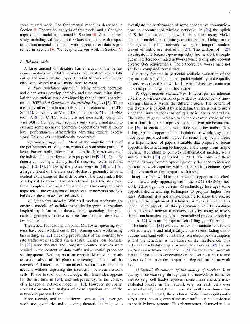
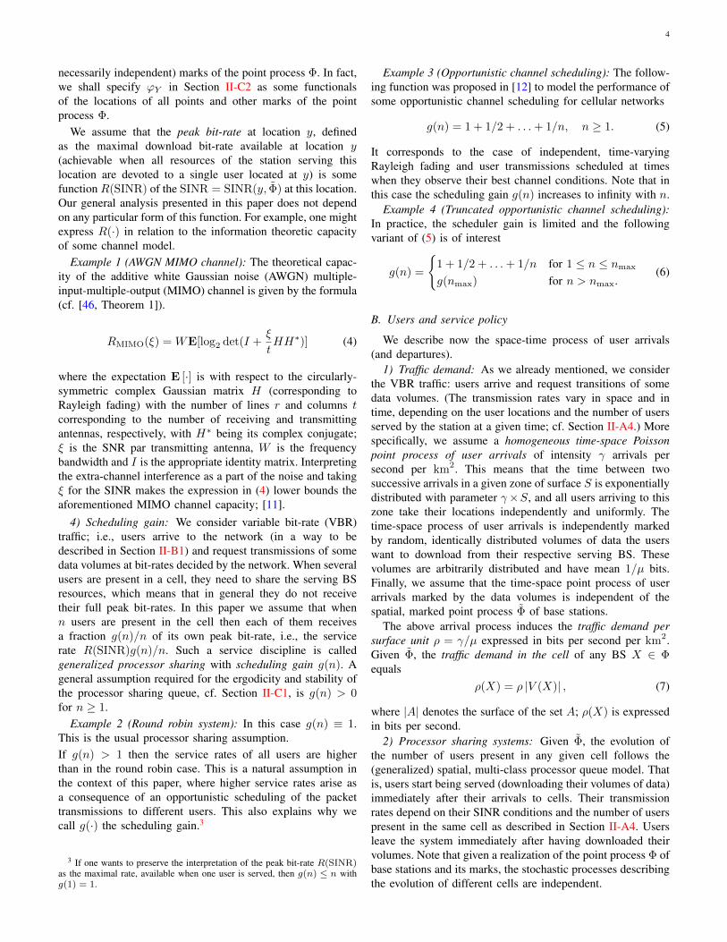
the round robin scheduler. Figure 1 shows that the generalizedprocessor sharing queue model with the considered truncatedopportunistic scheduler describes well the relation between thenumber of users and the cell load in the considered referencenetwork under different traffic conditions. The results are notsensitive to the choice nmax = 100 with very similar resultsobtained for nmax ≥ 20.

C. Estimation of the fixed parameters of the extended meancell model

We assume the truncated opportunistic scheduler validatedin Section IV-B, we place it in the context of our Poisson net-work model and estimate the parameters α, α′, c in (30), (31)and (32) of the extended mean cell model of Section III-B2.Figures 2(a) and (b) show the linear regression curves forthe SRSD parameters α and α′ of the traffic demand and thenormalized traffic demand, respectively. They confirm Fact 5and validate the first part of Observation 6. The second partof Observation 6, regarding the invariance with respect to thetraffic of the logarithmic correlation coefficient between thetraffic demand and the critical traffic demand is validated onFigure 2(c). We infer from this study the following estimatedvalues of these parameters:

α = 0.172057, α′ = 0.309799, c = −0.308575. (33)

Note that c < 0 meaning that the traffic demand ρ(0) andthe critical traffic demand ρc(0) are negatively correlated. Thiscan be explained by the fact that ρ(0) is proportional to thecell surface (18), while ρc(0) is the harmonic average of thepeak bit-rate function R(·) over the cell (17). For large cellsthis harmonic average is smaller due to small values of thepeak bit-rate far from the base station.

0 2 4 6

Traffic [kbit/s] square mean×107

0

2

4

6

8

10

12

Tra

ffic

[kb

it/s

] va

ria

nce

×106

Data

Linear fitting

(a) Liner regression for α

0 0.2 0.4 0.6 0.8

RhoPrime square mean

0

0.05

0.1

0.15

0.2

0.25

Rh

oP

rim

e v

aria

nce

Data

Linear fitting

(b) Liner regression for α′

0 2000 4000 6000 8000

Traffic mean [kbit/s]

-0.8

-0.6

-0.4

-0.2

0

0.2

Co

rre

latio

n

Data

Fitting

(c) logarithmic correlation coefficient c

Fig. 2: Linear regression estimation of the SRSD coefficients α and α′ on Figures (a)and (b), and the logarithmic correlation coefficient c on Figure (c), based on differentvalues of the mean traffic demand per cell in the simulated typical cell model.

D. Extended mean cell vs typical cell model

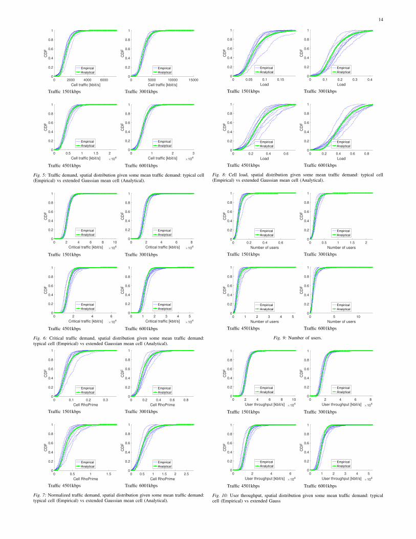
In this section we extensively validate the extended Gaus-sian mean cell model from Section III-B2 with respect to thedetailed typical cell model. We assume the parameters esti-mated in Section IV-C and study the cumulative distributionfunction (CDF) of several cell characteristics for the typicalcell and its extended Gaussian mean cell approximation.Figures 5, 6, 7, 8, 9, 10 (which are presented at the endof the paper) show the spatial CDF of the critical trafficdemand, normalized traffic demand, cell load, mean number ofusers and the user throughput, respectively, for different trafficregimes. The term “Empirical” and “Analytical” used in thelegends of these figures correspond to the CDF estimated bythe ergodic spatial averaging over the cells of the detailedmodel and the calculations made using the extended Gaussianmean cell model, respectively.

We conclude that the extended Gaussian mean cell modelis a good approximation of the typical cell model. It will beour main tool in the analysis of the real reference network.

E. Extended mean cell vs real data

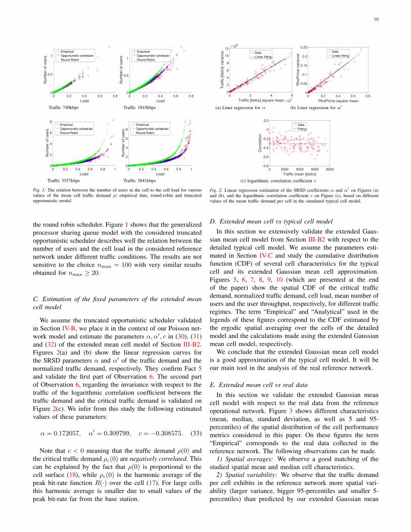
In this section we validate the extended Gaussian meancell model with respect to the real data from the referenceoperational network. Figure 3 shows different characteristics(mean, median, standard deviation, as well as 5 and 95-percentiles) of the spatial distribution of the cell performancemetrics considered in this paper. On these figures the term“Empirical” corresponds to the real data collected in thereference network. The following observations can be made.

1) Spatial averages: We observe a good matching of thestudied spatial mean and median cell characteristics.

2) Spatial variability: We observe that the traffic demandper cell exhibits in the reference network more spatial vari-ability (larger variance, bigger 95-percentiles and smaller 5-percentiles) than predicted by our extended Gaussian mean

11

0 2000 4000 6000 8000

Mean traffic per cell [kbit/s]

0

5000

10000

15000C

ell

tra

ffic

[kb

it/s

]

Mean, Empirical

Mean, Analytical

Std dev, Empirical

Std dev, Analytical

Quant 0.05, Empirical

Quant 0.05, Analytical



Traffic demand

0 2000 4000 6000 8000


0

1

2

3

4

Critica

l tr

aff

ic p

er

ce

ll [k

bit/s

] ×104

Mean, Empirical

Mean, Analytical

Std dev, Empirical

Std dev, Analytical





Critical traffic demand

0 2000 4000 6000 8000


0

0.5

1

1.5

2

Rh

oP

rim

e

Mean, Empirical

Mean, Analytical

Std dev, Empirical

Std dev, Analytical





Normalized traffic demand

0 2000 4000 6000 8000


0

0.2

0.4

0.6

0.8

1C

ell

loa

dMean, Empirical

Mean, Analytical

Std dev, Empirical

Std dev, Analytical





Cell load

0 2000 4000 6000 8000


0

0.5

1

1.5

2

Use

rs n

um

be

r p

er

ce

ll Mean, Empirical

Mean, Analytical

Median, Empirical

Median, Analytical





Number of users

0 2000 4000 6000 8000


0

1

2

3

4

Use

r th

rou

gh

pu

t p

er

ce

ll [k

bit/s

]

×104

Mean, Empirical

Mean, Analytical

Std dev, Empirical

Std dev, Analytical





User throughput

Fig. 3: Study of the spatial distribution of cell characteristics. Real data and the expendedmean cell model.

cell model. Assuming that the real reference network doesnot exhibit more spatial variability regarding the cell sizesthan our Poisson network model, the above observation mightsuggest that the real traffic demand process is not spatiallyhomogeneous. As a consequence the spatial variability of thecritical traffic demand, normalized traffic demand and the cellload calculated in the reference network is also bigger thanpredicted by the model. However, the differences between theempirical and analytical values of the variances and quantilesare in general much smaller than in the case of the trafficdemand, thus showing a relatively good agreement betweenthe model and the real data.

F. Throughput prediction

In this final numerical exercise we present on Figure 4 theprediction of the evolution of the mean user throughput in thereference network well beyond the currently observed trafficdemand (corresponding to “Empirical” points on the presentedfigure). The possibility to make such a prediction for variousfrequency spectra, density of base stations, scheduler, and link-layer technology (MIMO 2x2, 3x2 etc) is crucial for networkoperators for the strategic dimensioning planning. It allowsthem to estimate the required resources (and compare thecosts of these alternative solutions) to ensure that a sufficientlylarge fraction of the network (typically 95%) offers to user thetargeted throughput.

0 1 2 3

Mean traffic per cell [kbit/s] ×104

0

1

2

3

4

User

thro

ughput per

cell

[kbit/s

]

× 104

Mean, Empirical

Mean, Analytical

Std dev, Empirical

Std dev, Analytical





Fig. 4: Prediction of the evolution of the mean user throughout.

V. CONCLUSION

We have presented a comprehensive framework allowingcellular network operators to evaluate the performance oftheir networks and helping them to take strategic decisionsregarding network dimensioning.

It consists in a compound mathematical model based oninformation theory, queueing theory and stochastic geometry,whose elements can be configured to represent various layersof the given wireless cellular network. Evaluation of the modelrequires only static simulations to estimate some stochasticgeometric expectations which makes the proposed approachsignificantly more rapid than pure simulations often used bynetwork operators for this purpose.

We provide also a methodology allowing operators tocompare and keep the model adequate to the real data theysystematically collect in their networks, thus increasing thereliability of the network performance predictions.

Awaiting for more massive deployment of 5G networks toget more representative data, in an ongoing work we extendour framework to the analysis of this new wireless networktechnology.

ACKNOWLEDGEMENT

The authors would like to thank Mengting XIA for hercareful reading of the manuscript and for making variouscorrections and suggestions.

REFERENCES

[1] B. Błaszczyszyn, M. Jovanovic, and M. K. Karray, “Howuser throughput depends on the traffic demand in largecellular networks,” in Proc of WiOpt/SpaSWiN, 2014.

[2] B. Błaszczyszyn, R. Ibrahim, and M. Karray, “Spatialdisparity of QoS metrics between base stations in wire-less cellular networks,” IEEE Trans. Commun., vol. 64,no. 10, p. 4381, 2016, publised online 16 August 2016.

[3] 3GPP, “TR 36.814-V900 Further advancements for E-UTRA - Physical Layer Aspects,” in 3GPP Ftp Server,2010.

12

[4] G. Piro, L. A. Grieco, G. Boggia, F. Capozzi, andP. Camarda, “Simulating LTE cellular systems: an opensource framework,” IEEE Trans. Veh. Technol., vol. 60,pp. 498–513, 2011.

[5] C. Mehlfuhrer, J. C. Ikuno, M. Simko, S. Schwarz,M. Wrulich, and M. Rupp, “The Vienna LTE simulators- enabling reproducibility in wireless communicationsresearch,” EURASIP Journal on Advances in SignalProcessing, vol. 29, pp. 1–14, 2011.

[6] M. Simko, Q. Wang, and M. Rupp, “Optimal pilotsymbol power allocation under time-variant channels,”EURASIP Journal on Wireless Communications and Net-working, vol. 2012:225, no. 25, pp. 1–11, 2012.

[7] N. Baldo, M. Miozzo, M. Requena, and J. N. Guerrero,“An open source product-oriented LTE network simulatorbased on ns-3,” in Proc. of MSWIM, 2011.

[8] N. Baldo, M. Requena, J. Nin, and M. Miozzo, “A newmodel for the simulation of the LTE-EPC data plane,” inProc. of WNS3, 2012.

[9] A. J. Goldsmith and S.-G. Chua, “Variable-rate variable-power MQAM for fading channels,” IEEE Trans. Com-mun., vol. 45, pp. 1218–1230, 1997.

[10] P. E. Mogensen, W. Na, I. Z. Kovacs, F. Frederiksen,A. Pokhariyal, K. I. Pedersen, T. E. Kolding, K. Hugl,and M. Kuusela, “LTE capacity compared to the Shannonbound,” in Proc. of VTC Spring, 2007, pp. 1234–1238.

[11] M. K. Karray, M. Jovanovic, and B. Błaszczyszyn,“Theoretical expression of link performance in OFDMcellular networks with MIMO compared to simulationand measurements,” Annals of Telecommunications —Annales des Telecommunications, vol. 70, no. 11-12, pp.479–490, 2015.

[12] S. Borst, “User-level performance of channel-awarescheduling algorithms in wireless data networks,” inProceedings of INFOCOM 03, Mar. 2003.

[13] T. Bonald and A. Proutiere, “Wireless downlink datachannels: user performance and cell dimensioning,” inProc. of Mobicom, Sep. 2003.

[14] N. Hegde and E. Altman, “Capacity of multiserviceWCDMA networks with variable GoS,” in Proc. of IEEEWCNC, 2003.

[15] T. Bonald, S. C. Borst, N. Hegde, M. Jonckheere, andA. Proutiere, “Flow-level performance and capacity ofwireless networks with user mobility,” Queueing Systems,vol. 63, no. 1-4, pp. 131–164, 2009.

[16] L. Rong, S. E. Elayoubi, and O. B. Haddada, “Per-formance evaluation of cellular networks offering TVservices,” IEEE Trans. Veh. Technol., vol. 60, no. 2, pp.644 –655, feb. 2011.

[17] M. K. Karray and M. Jovanovic, “A queueing theoreticapproach to the dimensioning of wireless cellular net-works serving variable bit-rate calls,” IEEE Trans. Veh.Technol., vol. 62, no. 6, July 2013.

[18] J. Andrews, F. Baccelli, and R. Ganti, “A tractabl ap-proach to coverage and rate in cellular networks,” IEEETrans. Commun., vol. 59, no. 11, pp. 3122 –3134, novem-ber 2011.

[19] H. S. Dhillon, R. K. Ganti, F. Baccelli, and J. G.

Andrews, “Modeling and analysis of k-tier downlink het-erogeneous cellular networks,” IEEE Journal on SelectedAreas in Communications, vol. 30, no. 3, pp. 550–560,2012.

[20] B. Błaszczyszyn, M. Haenggi, P. Keeler, and S. Mukher-jee, Stochastic Geometry Analysis of Cellular Networks.Cambridge University Press, 2018.

[21] R. Serfozo, Introduction to stochastic networks.Springer Science & Business Media, 2012, vol. 44.

[22] F. Baccelli, B. Błaszczyszyn, and M. K. Karray, “Block-ing rates in large CDMA networks via a spatial Erlangformula,” in Proc. of IEEE INFOCOM, Miami, FL, USA,2005.

[23] B. Błaszczyszyn and M. K. Karray, “Performance eval-uation of scalable congestion control schemes for elastictraffic in cellular networks with power control,” in Proc.of IEEE INFOCOM, May 2007.

[24] I. Siomina and D. Yuan, “Analysis of cell load cou-pling for LTE network planning and optimization,” IEEETransactions on Wireless Communications, vol. 11, no. 6,pp. 2287–2297, 2012.

[25] Y. Zhou and W. Zhuang, “Performance analysis of co-operative communication in decentralized wireless net-works with unsaturated traffic,” IEEE Transactions onWireless Communications, vol. 15, no. 5, pp. 3518–3530,2016.

[26] M. Foruhandeh, N. Tadayon, and S. Aıssa, “Uplinkmodeling of k-tier heterogeneous networks: A queuingtheory approach,” IEEE Communications Letters, vol. 21,no. 1, pp. 164–167, 2017.

[27] Y. Zhong, T. Q. Quek, and X. Ge, “Heterogeneous cellu-lar networks with spatio-temporal traffic: Delay analysisand scheduling,” IEEE Journal on Selected Areas inCommunications, vol. 35, no. 6, pp. 1373–1386, 2017.

[28] J. Tian, H. Zhang, D. Wu, and D. Yuan, “QoS-constrained medium access probability optimization inwireless interference-limited networks,” IEEE Transac-tions on Communications, 2017.

[29] P. Viswanath, D. N. C. Tse, and R. Laroia, “Opportunisticbeamforming using dumb antennas,” IEEE transactionson information theory, vol. 48, no. 6, pp. 1277–1294,2002.

[30] A. Asadi and V. Mancuso, “A survey on opportunisticscheduling in wireless communications,” IEEE Commu-nications Surveys & Tutorials, vol. 15, no. 4, pp. 1671–1688, 2013.

[31] F. Berggren and R. Jantti, “Asymptotically fair transmis-sion scheduling over fading channels,” IEEE transactionson wireless communications, vol. 3, no. 1, pp. 326–336,2004.

[32] T. Ohto, K. Yamamoto, S.-L. Kim, T. Nishio, andM. Morikura, “Stochastic geometry analysis of normal-ized SNR-based scheduling in downlink cellular net-works,” IEEE Wireless Communications Letters, vol. 6,no. 4, pp. 438–441, 2017.

[33] K. Yamamoto, “Normalized SNR-based scheduling inpoisson networks,” private communication, 2018.

[34] W. L. Tan, F. Lam, and W. C. Lau, “An empirical study

13

on the capacity and performance of 3G networks,” IEEETransactions on Mobile Computing, vol. 7, no. 6, pp.737–750, 2008.

[35] D. Willkomm, S. Machiraju, J. Bolot, and A. Wolisz,“Primary users in cellular networks: A large-scale mea-surement study,” in New frontiers in dynamic spectrumaccess networks, 2008. DySPAN 2008. 3rd IEEE sympo-sium on. IEEE, 2008, pp. 1–11.

[36] U. Paul, A. P. Subramanian, M. M. Buddhikot, andS. R. Das, “Understanding traffic dynamics in cellulardata networks,” in INFOCOM, 2011 Proceedings IEEE.IEEE, 2011, pp. 882–890.

[37] M. Haenggi, “The meta distribution of the SIR in poissonbipolar and cellular networks,” IEEE Transactions onWireless Communications, vol. 15, no. 4, pp. 2577–2589,2016.

[38] F. Baccelli and B. Błaszczyszyn, “A new phase transi-tions for local delays in MANETs,” in INFOCOM, 2010Proceedings IEEE. IEEE, 2010, pp. 1–9.

[39] K. Majewski and M. Koonert, “Conservative cell loadapproximation for radio networks with shannon channelsand its application to LTE network planning,” in Telecom-munications (AICT), 2010 Sixth Advanced InternationalConference on. IEEE, 2010, pp. 219–225.

[40] Z. Niu, Y. Wu, J. Gong, and Z. Yang, “Cell zooming forcost-efficient green cellular networks,” IEEE communi-cations magazine, vol. 48, no. 11, 2010.

[41] H. Zhang, X. Qiu, L. Meng, and X. Zhang, “Designof distributed and autonomic load balancing for self-organization LTE,” in Vehicular technology conferencefall (VTC 2010-Fall), 2010 IEEE 72nd. IEEE, 2010,pp. 1–5.

[42] B. Błaszczyszyn, M. Jovanovic, and M. K. Karray, “Per-formance laws of large heterogeneous cellular networks,”in In proc. of WiOpt/SpaSWiN, 2015.

[43] B. Błaszczyszyn and M. K. Karray, “What frequencybandwidth to run cellular network in a given coun-try? — a downlink dimensioning problem,” in Proc. ofWiOpt/SpaSWiN, 2015.

[44] M. Jovanovic, M. K. Karray, and B. Błaszczyszyn, “QoSand network performance estimation in heterogeneouscellular networks validated by real-field measurements,”in Proc. of ACM PM2HW2N, Montreal, Canada, 2014.

[45] D. J. Daley and D. VereJones, An introduction to thetheory of point processes. Volume I, 2nd ed. New York:Springer, 2003.

[46] I. E. Telatar, “Capacity of multiple antenna Gaussianchannels,” AT&T Technical Memorandum, June 1995.

[47] J. W. Cohen, “The multiple phase service network withgeneralized processor sharing,” Acta informatica, no. 3,pp. 245–284, 1979.

[48] F. P. Kelly, Reversibility and stochastic networks. Cam-bridge University Press, 2011.

[49] F. Baccelli and B. Błaszczyszyn, Stochastic Geometryand Wireless Networks, Volume I — Theory, ser. Foun-dations and Trends in Networking. NoW Publishers,2009, vol. 3, No 3–4.

[50] H. P. Keeler, B. Błaszczyszyn, and M. K. Karray, “SINR-

based k-coverage probability in cellular networks witharbitrary shadowing,” in Proc. of IEEE ISIT, 2013.

[51] H. P. Keeler and B. Błaszczyszyn, “SINR in wireless net-works and the two-parameter Poisson-Dirichlet process,”IEEE Wireless Comm Letters, vol. 3, no. 5, pp. 525–528,2014.

[52] B. Błaszczyszyn and H. P. Keeler, “Studying the SINRprocess of the typical user in Poisson networks by usingits factorial moment measures,” IEEE Trans. Inf. Theory,2015.

[53] I. Nakata and N. Miyoshi, “Spatial stochastic models foranalysis of heterogeneous cellular networks with repul-sively deployed base stations,” Performance Evaluation,vol. 78, pp. 7–17, 2014.

[54] N. Miyoshi and T. Shirai, “Cellular networks with α-Ginibre configurated base stations,” in The Impact ofApplications on Mathematics. Springer, 2014, pp. 211–226.

[55] N. Deng, W. Zhou, and M. Haenggi, “The Ginibre pointprocess as a model for wireless networks with repulsion,”IEEE Transactions on Wireless Communications, vol. 14,no. 1, pp. 107–121, 2015.

14

0 2000 4000 6000

Cell traffic [kbit/s]

0

0.2

0.4

0.6

0.8

1

CD

F

Empirical

Analytical

Traffic 1501kbps

0 5000 10000 15000

Cell traffic [kbit/s]

0

0.2

0.4

0.6

0.8

1

CD

F

Empirical

Analytical

Traffic 3001kbps

0 0.5 1 1.5 2

Cell traffic [kbit/s] ×104

0

0.2

0.4

0.6

0.8

1

CD

F

Empirical

Analytical

Traffic 4501kbps

0 1 2 3

Cell traffic [kbit/s] ×104

0

0.2

0.4

0.6

0.8

1

CD

F

Empirical

Analytical

Traffic 6001kbps

Fig. 5: Traffic demand, spatial distribution given some mean traffic demand: typical cell(Empirical) vs extended Gaussian mean cell (Analytical).

0 2 4 6 8 10

Critical traffic [kbit/s] ×104

0

0.2

0.4

0.6

0.8

1

CD

F

Empirical

Analytical

Traffic 1501kbps

0 2 4 6 8


0

0.2

0.4

0.6

0.8

1

CD

F

Empirical

Analytical

Traffic 3001kbps

0 2 4 6


0

0.2

0.4

0.6

0.8

1

CD

F

Empirical

Analytical

Traffic 4501kbps

0 1 2 3 4 5


0

0.2

0.4

0.6

0.8

1

CD

F

Empirical

Analytical

Traffic 6001kbps

Fig. 6: Critical traffic demand, spatial distribution given some mean traffic demand:typical cell (Empirical) vs extended Gaussian mean cell (Analytical).

0 0.1 0.2 0.3

Cell RhoPrime

0

0.2

0.4

0.6

0.8

1

CD

F

Empirical

Analytical

Traffic 1501kbps

0 0.2 0.4 0.6 0.8

Cell RhoPrime

0

0.2

0.4

0.6

0.8

1

CD

F

Empirical

Analytical

Traffic 3001kbps

0 0.5 1 1.5

Cell RhoPrime

0

0.2

0.4

0.6

0.8

1

CD

F

Empirical

Analytical

Traffic 4501kbps

0 0.5 1 1.5 2 2.5

Cell RhoPrime

0

0.2

0.4

0.6

0.8

1

CD

F

Empirical

Analytical

Traffic 6001kbps

Fig. 7: Normalized traffic demand, spatial distribution given some mean traffic demand:typical cell (Empirical) vs extended Gaussian mean cell (Analytical).

0 0.05 0.1 0.15

Load

0

0.2

0.4

0.6

0.8

1

CD

F

Empirical

Analytical

Traffic 1501kbps

0 0.1 0.2 0.3 0.4

Load

0

0.2

0.4

0.6

0.8

1

CD

F

Empirical

Analytical

Traffic 3001kbps

0 0.2 0.4 0.6

Load

0

0.2

0.4

0.6

0.8

1

CD

F

Empirical

Analytical

Traffic 4501kbps

0 0.2 0.4 0.6 0.8

Load

0

0.2

0.4

0.6

0.8

1

CD

F

Empirical

Analytical

Traffic 6001kbps

Fig. 8: Cell load, spatial distribution given some mean traffic demand: typical cell(Empirical) vs extended Gaussian mean cell (Analytical).

0 0.2 0.4 0.6

Number of users

0

0.2

0.4

0.6

0.8

1

CD

F

Empirical

Analytical

Traffic 1501kbps

0 0.5 1 1.5 2

Number of users

0

0.2

0.4

0.6

0.8

1

CD

F

Empirical

Analytical

Traffic 3001kbps

0 1 2 3 4 5

Number of users

0

0.2

0.4

0.6

0.8

1

CD

F

Empirical

Analytical

Traffic 4501kbps

0 5 10

Number of users

0

0.2

0.4

0.6

0.8

1

CD

FEmpirical

Analytical

Traffic 6001kbps

Fig. 9: Number of users.

0 2 4 6 8 10

User throughput [kbit/s] ×104

0

0.2

0.4

0.6

0.8

1

CD

F

Empirical

Analytical

Traffic 1501kbps

0 2 4 6 8


0

0.2

0.4

0.6

0.8

1

CD

F

Empirical

Analytical

Traffic 3001kbps

0 2 4 6


0

0.2

0.4

0.6

0.8

1

CD

F

Empirical

Analytical

Traffic 4501kbps

0 1 2 3 4 5


0

0.2

0.4

0.6

0.8

1

CD

F

Empirical

Analytical

Traffic 6001kbps

Fig. 10: User throughput, spatial distribution given some mean traffic demand: typicalcell (Empirical) vs extended Gauss

performance analysis of cellular networks with

Documents