percept implementation character recognition
DESCRIPTION
A simple method to implement a perceptor neural network for character recognition purposes.TRANSCRIPT

POLYTECHNIC UNIVERSITYDepartment of Computer and Information Science
Perceptron for PatternClassification
K. Ming Leung
Abstract: A neural network, known as the perceptron,capable of classifying patterns into two or more cate-gories is introduced. The network is trained using theperceptron learning rule.
Directory• Table of Contents• Begin Article
Copyright c© 2008 [email protected] Revision Date: February 13, 2008

Table of Contents
1. Simple Perceptron for Pattern Classification
2. Application: Bipolar Logical Function: AND
3. Perceptron Learning Rule Convergence Theorem
4. Perceptron for Multi-Category Classification
5. Example of a Perceptron with Multiple Output Neurons

Section 1: Simple Perceptron for Pattern Classification 3
1. Simple Perceptron for Pattern Classification
We consider here a NN, known as the Perceptron, which is capableof performing pattern classification into two or more categories. Theperceptron is trained using the perceptron learning rule. We will firstconsider classification into two categories and then the general multi-class classification later.
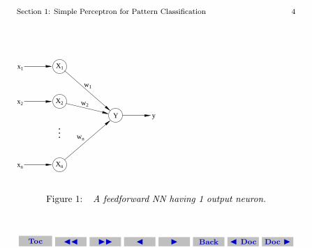
For classification into only two categories, all we need is a singleoutput neuron. Here we will use bipolar neurons. The simplest archi-tecture that could do the job consists of a layer of N input neurons,an output layer with a single output neuron, and no hidden layers.This is the same architecture as we saw before for Hebb learning.
However, we will use a different transfer function here for the out-put neuron:
fθ(x) =
+1, if x > θ,
0, if − θ ≤ x ≤ θ,−1, if x < −θ.
This transfer function has an undecided band of width 2θ. The value
Toc JJ II J I Back J Doc Doc I
Section 1: Simple Perceptron for Pattern Classification 4
X1
X2
Xn
Y
x1
x2
xn
y
w1
w2
wn
Figure 1: A feedforward NN having 1 output neuron.
Toc JJ II J I Back J Doc Doc I
Section 1: Simple Perceptron for Pattern Classification 5
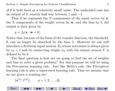
of θ is held fixed at a relatively small value. The undecided case hasan output of 0, exactly half way between 1 and −1.
Thus if we represent the N components of the input vector by x,the N components of the weight vector by w, and the bias by b, theoutput is then given by
y = fθ(x ·w + b).
Notice that because of the form of the transfer function, the threshold,θ, can no longer be absorbed by the bias, b. However we can stillintroduce a fictitious input neuron X0 whose activation is always givenby x0 = 1 and its connecting weight w0 with the output neuron Y isdefined to be b.
The final question is how are we going to find the set of weightsand bias to solve a given problem? For this purpose we will be usingthe Perceptron learning rule. Just like Hebb’s rule, the Perceptronlearning rule is also a supervised learning rule. Thus we assume thatwe are given a training set:
{s(q), t(q)}, q = 1, 2, . . . , Q.
Toc JJ II J I Back J Doc Doc I

Section 1: Simple Perceptron for Pattern Classification 6
where s(q) is a training vector, and t(q) is its corresponding targetedoutput value.
Toc JJ II J I Back J Doc Doc I
Section 1: Simple Perceptron for Pattern Classification 7
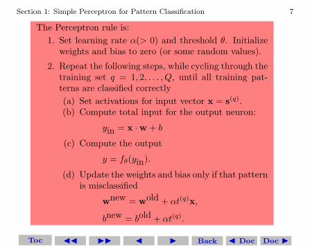
The Perceptron rule is:1. Set learning rate α(> 0) and threshold θ. Initialize
weights and bias to zero (or some random values).
2. Repeat the following steps, while cycling through thetraining set q = 1, 2, . . . , Q, until all training pat-terns are classified correctly(a) Set activations for input vector x = s(q).(b) Compute total input for the output neuron:
yin = x ·w + b
(c) Compute the output
y = fθ(yin).
(d) Update the weights and bias only if that patternis misclassified
wnew = wold + αt(q)x,
bnew = bold + αt(q).
Toc JJ II J I Back J Doc Doc I
Section 2: Application: Bipolar Logical Function: AND 8
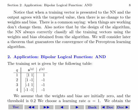
Notice that when a training vector is presented to the NN and theoutput agrees with the targeted value, then there is no change to theweights and bias. There is a common saying: when things are workingdon’t change them. Also notice that by the design of the algorithm,the NN always correctly classify all the training vectors using theweights and bias obtained from the algorithm. We will consider latera theorem that guarantees the convergence of the Perceptron learningalgorithm.
2. Application: Bipolar Logical Function: AND
The training set is given by the following table:
q s(q) t(q)
1 [1 1] 12 [1 -1] -13 [-1 1] -14 [-1 -1] -1
We assume that the weights and bias are initially zero, and thethreshold is 0.2 We choose a learning rate α = 1. We obtain the
Toc JJ II J I Back J Doc Doc I
Section 2: Application: Bipolar Logical Function: AND 9
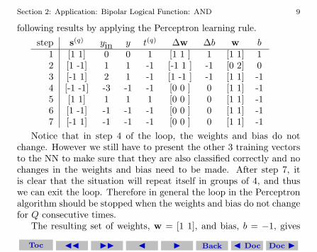
following results by applying the Perceptron learning rule.
step s(q) yin y t(q) ∆w ∆b w b1 [1 1] 0 0 1 [1 1 ] 1 [1 1] 12 [1 -1] 1 1 -1 [-1 1 ] -1 [0 2] 03 [-1 1] 2 1 -1 [1 -1 ] -1 [1 1] -14 [-1 -1] -3 -1 -1 [0 0 ] 0 [1 1] -15 [1 1] 1 1 1 [0 0 ] 0 [1 1] -16 [1 -1] -1 -1 -1 [0 0 ] 0 [1 1] -17 [-1 1] -1 -1 -1 [0 0 ] 0 [1 1] -1
Notice that in step 4 of the loop, the weights and bias do notchange. However we still have to present the other 3 training vectorsto the NN to make sure that they are also classified correctly and nochanges in the weights and bias need to be made. After step 7, itis clear that the situation will repeat itself in groups of 4, and thuswe can exit the loop. Therefore in general the loop in the Perceptronalgorithm should be stopped when the weights and bias do not changefor Q consecutive times.
The resulting set of weights, w = [1 1], and bias, b = −1, gives
Toc JJ II J I Back J Doc Doc I
Section 2: Application: Bipolar Logical Function: AND 10
the decision boundary determined by
x1w1 + x2w2 = x1 + x2 = 1.
This boundary is a straight line given by
x2 = 1− x1,
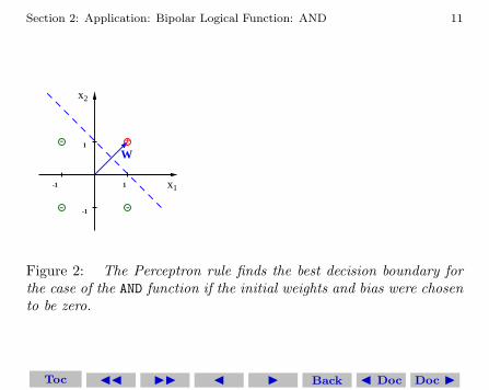
which has a slope of −1 and passes through the point [1 0]. This isthe best decision boundary for this problem in terms of robustness(the training vectors are farthest from the decision boundary). Thusin this example, the Perceptron learning algorithm converges to a setof weights and bias that is the best choice for this NN.
However this is all quite fortuitous. In general we cannot expectthe Perceptron learning algorithm to converge to a set of weights andbias that is the best choice for any given NN. It is easy to see thatbecause if we had assumed some none zero values for the initial weightsor bias, in all likelihood we would not have gotten the best decisionboundary for this problem.
Toc JJ II J I Back J Doc Doc I
Section 2: Application: Bipolar Logical Function: AND 11
x1
x2
W+
-
-
-
1-1
1
-1
Figure 2: The Perceptron rule finds the best decision boundary forthe case of the AND function if the initial weights and bias were chosento be zero.
Toc JJ II J I Back J Doc Doc I

Section 3: Perceptron Learning Rule Convergence Theorem 12
3. Perceptron Learning Rule Convergence Theorem
To consider the convergence theorem for the Perceptron LearningRule, it is convenient to absorb the bias by introducing an extra inputneuron, X0, whose signal is always fixed to be unity.
Convergence Theorem for the Perceptron Learning Rule:For a Perceptron, if there is a correct weight vector w∗
that gives correct response for all training patterns, thatis
fθ(s(q) ·w∗) = t(q), ∀q = 1, . . . , Q,
then for any starting weight vector w, the Perceptronlearning rule will converge in a finite number of steps to acorrect weight vector.
According to the theorem, a table like the one given above for theNN functioning as an AND gate, must terminate after a finite numberof steps. Note that the vectors appearing in the second column areall chosen from the training set. The same vector may appear more
Toc JJ II J I Back J Doc Doc I

Section 3: Perceptron Learning Rule Convergence Theorem 13
that once in that column. First we can ignore from that column thosevectors that are classified correctly at the particular point in the loop,since they lead to no changes in the weights or the bias. Next, Weconsider those vectors in that column, say s(q). whose target outputis t(q) = −1. This means that we want s(q) · w < −θ so that theoutput y = −1. If we multiply this inequality by minus one, we have−s(q) ·w > θ. We can reverse the signs of all these vectors so that wewant their target output to be +1.
We denote the list of these vectors by F . The individual vectorsare denoted by x(k), so that
F = {x(0),x(1), . . . ,x(n), . . .}.Out goal is to prove that this list must terminate after a finite numberof steps, and therefore contains only a finite number of vectors. Bydesign, all these vectors have target outputs of +1, and they are allincorrectly classified at their own step in the loop.
The initial weight is w(0), and at step n (not counting those stepswhere the training vectors presented to the NN are classified correctly)the weight vector is w(n). Therefore for any n, x(n) is misclassified
Toc JJ II J I Back J Doc Doc I

Section 3: Perceptron Learning Rule Convergence Theorem 14
by definition and therefore we always have x(n) ·w(n) < 0.We let w∗ be a correct weight vector assuming that there is such
a vector. Then by the fact that w∗ gives a decision boundary thatcorrectly classifies all the training vectors in F , we have
x(n) ·w∗ > 0, ∀x(n) ∈ F .We need to define the following two quantities to be used in the proof:
m = minx(n)∈F
x(n) ·w∗,
M = maxx(n)∈F
‖x(n)‖2.
Notice that both quantities are strictly positive.Now we want to prove that the number of steps in the Perceptron
learning rule is always finite provided that w∗ exists.For this proof, we assume that θ = 0.The first step in the loop of the Perceptron learning rule gives
w(1) = w(0) + αx(0),
Toc JJ II J I Back J Doc Doc I

Section 3: Perceptron Learning Rule Convergence Theorem 15
and the second step gives
w(2) = w(1) + αx(1) = w(0) + αx(0) + αx(1).
Thus after k steps, we have
w(k) = w(0) + α
k−1∑n=0
x(n).
We take the dot-product of this equation with w∗ to give
w(k) ·w∗ = w(0) ·w∗ + α
k−1∑n=0
x(n) ·w∗.
But by the definition of m, we have x(n) ·w∗ ≥ m for any n. So wehave the inequality
w(k) ·w∗ > w(0) ·w∗ + α
k−1∑n=0
m = w(0) ·w∗ + αkm.
Notice that in the above relation, equality is not possible becausethere is at least one vector x(p) in the sum such that x(p) ·w∗ > m.
Toc JJ II J I Back J Doc Doc I
Section 3: Perceptron Learning Rule Convergence Theorem 16
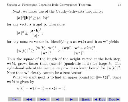
Next, we make use of the Cauchy-Schwartz inequality:
‖a‖2‖b‖2 ≥ (a · b)2
for any vectors a and b. Therefore
‖a‖2 ≥ (a · b)2
‖b‖2,
for any nonzero vector b. Identifying a as w(k) and b as w∗ yields
‖w(k)‖2 ≥ (w(k) ·w∗)2
‖w∗‖2>
(w(0) ·w∗ + αkm)2
‖w∗‖2.
Thus the square of the length of the weight vector at the k-th step,w(k), grows faster than (αkm)2 (quadratic in k) for large k. Theright-hand side of the inequality provides a lower bound for ‖w(k)‖2.Note that w∗ clearly cannot be a zero vector.
What we want next is to find an upper bound for ‖w(k)‖2. Sincew(k) is given by
w(k) = w(k − 1) + αx(k − 1),
Toc JJ II J I Back J Doc Doc I

Section 3: Perceptron Learning Rule Convergence Theorem 17
taking the dot-product with itself gives
‖w(k)‖2 = ‖w(k− 1)‖2 +α2‖x(k− 1)‖2 + 2αx(k− 1) ·w(k− 1).
Since x(k−1) ·w(k−1) must be negative because x(k−1) is classifiedincorrectly, the last term on the right-hand side of the above equationcan be omitted to obtain the inequality
‖w(k)‖2 < ‖w(k − 1)‖2 + α2‖x(k − 1)‖2.Replacing k by k − 1 gives
‖w(k − 1)‖2 < ‖w(k − 2)‖2 + α2‖x(k − 2)‖2.Using this above inequality to eliminate ‖w(k − 1)‖2 yields
‖w(k)‖2 < ‖w(k − 2)‖2 + α2‖x(k − 2)‖2 + α2‖x(k − 1)‖2.This procedure can be iterated to give
‖w(k)‖2 < ‖w(0)‖2+α2‖x(0)‖2+. . .+α2‖x(k−2)‖2+α2‖x(k−1)‖2.Using the definition of M , we have the inequality
‖w(k)‖2 < ‖w(0)‖2 + α2kM.
Toc JJ II J I Back J Doc Doc I
Section 3: Perceptron Learning Rule Convergence Theorem 18
This inequality gives an upper bound for the square of w(k), andshows that it cannot grow faster than α2kM (linear in k).
Combining this upper bound with the lower bound for ‖w(k)‖2,we have
(w(0) ·w∗ + αkm)2
‖w∗‖2≤ ‖w(k)‖2 ≤ ‖w(0)‖2 + α2kM.
This bound is clearly valid initially when k = 0, because in thatcase the bound is
(w(0) · w∗)2 ≤ ‖w(0)‖2 ≤ ‖w(0)‖2.Notice that the square of the projection of w(0) in any direction can-not be larger than ‖w(0)‖2.
Next consider what happens as k increases. Since the lower boundgrows faster (quadratically with k) than the upper bound, which growsonly linearly with k, there must be a value of k∗ such that this con-dition is violated for all k ≥ k∗. This means the iteration cannotcontinue forever and must therefore terminate after k∗ steps.
To determine k∗, let κ be a solution of the following quadratic
Toc JJ II J I Back J Doc Doc I
Section 3: Perceptron Learning Rule Convergence Theorem 19
equation
(w(0) ·w∗ + ακm)2
‖w∗‖2= ‖w(0)‖2 + α2κM.
We find that κ is given by
κ =R
2−D ±
√R2
4−RD + L2,
where we have defined
R =maxx(n)∈F{x(n) · x(n)}(minx(n)∈F{x(n) · w∗}
)2 ,D =
w(0) · w∗
αminx(n)∈F{x(n) · w∗},
L2 =‖w(0)‖2
α2(minx(n)∈F{x(n) · w∗}
)2 .In these expressions, w∗ is a unit vector (having unit magnitude)pointing in the direction of w∗.
Toc JJ II J I Back J Doc Doc I
Section 3: Perceptron Learning Rule Convergence Theorem 20
We want to show that only the upper sign leads to acceptablesolution. First we assume that R
2 −D is positive. Clearly the uppersign will give a positive κ as required. The lower sign will lead to anunacceptable negative κ. We can prove that by showing that
R
2−D <
√R2
4−RD + L2.
Since both sides of this inequality are positive, we can square bothsides to give(
R
2−D
)2
=R2
4−RD +D2 <
R2
4−RD + L2.
This relation becomesD2 < L2 or equivalently(w(0) · w∗
)2< ‖w(0)‖2.
This final relation is obviously true because the square of the projec-tion of any vector in any direction cannot be larger than the magnitudesquare of the vector itself.
Next we assume that R2 −D is negative. Then the lower sign will
always give a negative κ. On the other hand, the upper sign will
Toc JJ II J I Back J Doc Doc I

Section 4: Perceptron for Multi-Category Classification 21
always give an acceptable positive κ because√R2
4−RD + L2 > −
(R
2−D
),
as can be seen by squaring both sides.Our conclusion is that k∗ is given by dκe where
κ =R
2−D +
√R2
4−RD + L2.
If the weight vector is initialized to zero, then D = L = 0 andtherefore k∗ = dκe = dRe. From the definition of R, we see thatthe number of iteration is determined by the training vector that lieclosest to the decision boundary. The smaller that distance is thehigher the number of iterations has to be for convergence.
4. Perceptron for Multi-Category Classification
We will now extend to the case where a NN has to be able to classifyinput vectors, each having N components, into more than 2 categories.
Toc JJ II J I Back J Doc Doc I
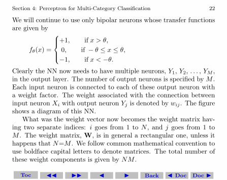
Section 4: Perceptron for Multi-Category Classification 22
We will continue to use only bipolar neurons whose transfer functionsare given by
fθ(x) =
+1, if x > θ,
0, if − θ ≤ x ≤ θ,−1, if x < −θ.
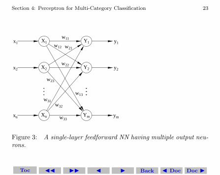
Clearly the NN now needs to have multiple neurons, Y1, Y2, . . . , YM ,in the output layer. The number of output neurons is specified by M .Each input neuron is connected to each of these output neuron witha weight factor. The weight associated with the connection betweeninput neuron Xi with output neuron Yj is denoted by wij . The figureshows a diagram of this NN.
What was the weight vector now becomes the weight matrix hav-ing two separate indices: i goes from 1 to N , and j goes from 1 toM . The weight matrix, W, is in general a rectangular one, unless ithappens that N=M . We follow common mathematical convention touse boldface capital letters to denote matrices. The total number ofthese weight components is given by NM .
Toc JJ II J I Back J Doc Doc I
Section 4: Perceptron for Multi-Category Classification 23
X1
X2
Xn
Y1
Y2
Ym
x1
x2
xn
y1
y2
ym
w11
w12
w13
w21
w22
w23
w31w32
w33
Figure 3: A single-layer feedforward NN having multiple output neu-rons.
Toc JJ II J I Back J Doc Doc I
Section 4: Perceptron for Multi-Category Classification 24
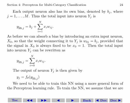
Each output neuron also has its own bias, denoted by bj , wherej = 1, . . . ,M . Thus the total input into neuron Yj is
yin,j = bj +N∑i=1
xiwij .
As before we can absorb a bias by introducing an extra input neuron,X0, so that the weight connecting it to Yj is w0j = bj , provided thatthe signal in X0 is always fixed to be x0 = 1. Then the total inputinto neuron Yj can be rewritten as
yin,j =N∑i=0
xiwij .
The output of neuron Yj is then given by
yj = fθ(yin,j)
We need to be able to train this NN using a more general form ofthe Perceptron learning rule. To train the NN, we assume that we are
Toc JJ II J I Back J Doc Doc I
Section 4: Perceptron for Multi-Category Classification 25
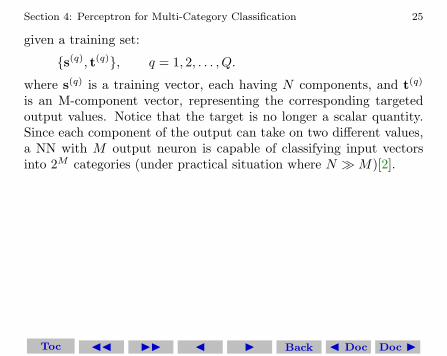
given a training set:
{s(q), t(q)}, q = 1, 2, . . . , Q.
where s(q) is a training vector, each having N components, and t(q)
is an M-component vector, representing the corresponding targetedoutput values. Notice that the target is no longer a scalar quantity.Since each component of the output can take on two different values,a NN with M output neuron is capable of classifying input vectorsinto 2M categories (under practical situation where N �M)[2].
Toc JJ II J I Back J Doc Doc I
Section 4: Perceptron for Multi-Category Classification 26
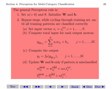
The general Perceptron rule is:1. Set α(> 0) and θ. Initialize W and b.
2. Repeat steps, while cycling through training set, un-til all training patterns are classified correctly
(a) Set input vector xi = s(q)i , i = 1, . . . , N .
(b) Compute total input for each output neuron:
yin,j =N∑i=1
xiwij + bj , j = 1, . . . ,M.
(c) Compute the output
yj = fθ(yin,j), j = 1, . . . ,M.
(d) Update W and b only if pattern is misclassified
wnewij = wold
ij + αxit(q)j ,
bnewj = bold
j + αt(q)j .
Toc JJ II J I Back J Doc Doc I
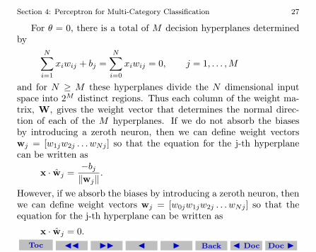
Section 4: Perceptron for Multi-Category Classification 27
For θ = 0, there is a total of M decision hyperplanes determinedby
N∑i=1
xiwij + bj =N∑i=0
xiwij = 0, j = 1, . . . ,M
and for N ≥ M these hyperplanes divide the N dimensional inputspace into 2M distinct regions. Thus each column of the weight ma-trix, W, gives the weight vector that determines the normal direc-tion of each of the M hyperplanes. If we do not absorb the biasesby introducing a zeroth neuron, then we can define weight vectorswj = [w1jw2j . . . wNj ] so that the equation for the j-th hyperplanecan be written as
x · wj =−bj‖wj‖
.
However, if we absorb the biases by introducing a zeroth neuron, thenwe can define weight vectors wj = [w0jw1jw2j . . . wNj ] so that theequation for the j-th hyperplane can be written as
x · wj = 0.Toc JJ II J I Back J Doc Doc I
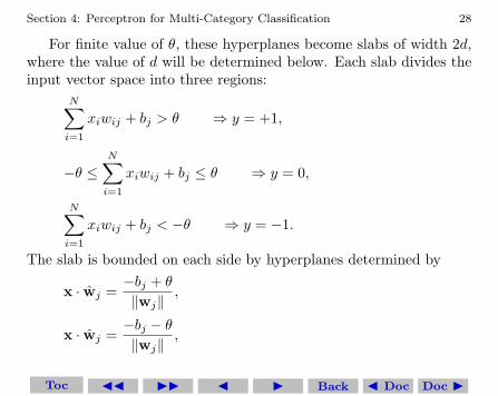
Section 4: Perceptron for Multi-Category Classification 28
For finite value of θ, these hyperplanes become slabs of width 2d,where the value of d will be determined below. Each slab divides theinput vector space into three regions:
N∑i=1
xiwij + bj > θ ⇒ y = +1,
−θ ≤N∑i=1
xiwij + bj ≤ θ ⇒ y = 0,
N∑i=1
xiwij + bj < −θ ⇒ y = −1.
The slab is bounded on each side by hyperplanes determined by
x · wj =−bj + θ
‖wj‖,
x · wj =−bj − θ‖wj‖
,
Toc JJ II J I Back J Doc Doc I

Section 4: Perceptron for Multi-Category Classification 29
where the weight vectors are defined by wj = [w1jw2j . . . wNj ]. There-fore the slab has a thickness 2dj , where
dj =θ
‖wj‖.
However, if we absorb the biases by introducing a zeroth neuron, thenthe slab is bounded on each side by hyperplanes determined by
x · wj =θ
‖wj‖,
x · wj =−θ‖wj‖
,
where the weight vectors are now defined by wj = [w0jw1jw2j . . . wNj ].Therefore the slab has a thickness 2dj , where
dj =θ
‖wj‖.
Although this expression for dj looks identical to the one above, theweight vectors are defined slightly differently, and the slab is located
Toc JJ II J I Back J Doc Doc I

Section 5: Example of a Perceptron with Multiple Output Neurons 30
Wj
/|Wj|
/|Wj|x1
x2
Figure 4: A hyperplane with a safety margin.
in an input vector space one higher than the one before. The figureshows one of the hyperplanes with a safety margin.
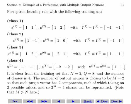
5. Example of a Perceptron with Multiple Output Neurons
We consider the following Perceptron with multiple output units. Wewant to design a NN, using bipolar neurons, and train it using the
Toc JJ II J I Back J Doc Doc I
Section 5: Example of a Perceptron with Multiple Output Neurons 31
Perceptron learning rule with the following training set:
(class 1)
s(1) =[
1 1], s(2) =
[1 2
]with t(1) = t(2) =
[−1 −1
](class 2)
s(3) =[
2 −1], s(4) =
[2 0
]with t(3) = t(4) =
[−1 1
](class 3)
s(5) =[−1 2
], s(6) =
[−2 1
]with t(5) = t(6) =
[1 −1
](class 4)
s(7) =[−1 −1
], s(8) =
[−2 −2
]with t(7) = t(8) =
[1 1
]It is clear from the training set that N = 2, Q = 8, and the numberof classes is 4. The number of output neuron is chosen to be M = 2so that each target vector has 2 components, each of which taking on2 possible values, and so 2M = 4 classes can be represented. (Notethat M 6> N here.)
Toc JJ II J I Back J Doc Doc I

Section 5: Example of a Perceptron with Multiple Output Neurons 32
Setting α = 1 and θ = 0, and assuming zero initial weights andbiases, we find that the Perceptron algorithm converges after 11 iter-ations (a little more than 1 epoch through the training set) to give
W =[−3 1
0 −2
], b =
[−2 0
].
The 2 decision boundaries are given by the equations
−3x1 − 2 = 0, x1 − 2x2 = 0,
which correspond to the following 2 straight lines through the origin
x1 = −23, x2 =
12x1.
These 2 lines separate the input vector space into 4 regions and it iseasy to see that the NN correctly classifies the 8 training vectors into4 classes. However these boundaries are not the most robust againstrandom fluctuations in the components of the input vectors.
Here we have chosen a threshold θ = 0. One expects that for alarger value of θ, a more robust set of decision slabs can be obtained.Experimentation by keeping α = 1 but using larger values of θ shows
Toc JJ II J I Back J Doc Doc I

Section 5: Example of a Perceptron with Multiple Output Neurons 33
−3 −2 −1 0 1 2 3−3
−2
−1
0
1
2
3
s(1)
s(2)
s(3)
s(4)
s(5)
s(6)
s(7)
s(8)
s(1)
s(2)
s(3)
s(4)
s(5)
s(6)
s(7)
s(8)
s(1)
s(2)
s(3)
s(4)
s(5)
s(6)
s(7)
s(8)
s(1)
s(2)
s(3)
s(4)
s(5)
s(6)
s(7)
s(8)
s(1)
s(2)
s(3)
s(4)
s(5)
s(6)
s(7)
s(8)
s(1)
s(2)
s(3)
s(4)
s(5)
s(6)
s(7)
s(8)
s(1)
s(2)
s(3)
s(4)
s(5)
s(6)
s(7)
s(8)
s(1)
s(2)
s(3)
s(4)
s(5)
s(6)
s(7)
s(8)
Decision hyperplanes for θ = 0
x1
x 2
Figure 5: A Perceptron capable of classifying patterns into 4 classes.
Toc JJ II J I Back J Doc Doc I
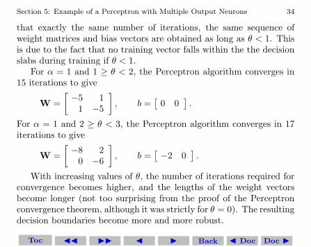
Section 5: Example of a Perceptron with Multiple Output Neurons 34
that exactly the same number of iterations, the same sequence ofweight matrices and bias vectors are obtained as long as θ < 1. Thisis due to the fact that no training vector falls within the the decisionslabs during training if θ < 1.
For α = 1 and 1 ≥ θ < 2, the Perceptron algorithm converges in15 iterations to give
W =[−5 1
1 −5
], b =
[0 0
].
For α = 1 and 2 ≥ θ < 3, the Perceptron algorithm converges in 17iterations to give
W =[−8 2
0 −6
], b =
[−2 0
].
With increasing values of θ, the number of iterations required forconvergence becomes higher, and the lengths of the weight vectorsbecome longer (not too surprising from the proof of the Perceptronconvergence theorem, although it was strictly for θ = 0). The resultingdecision boundaries become more and more robust.
Toc JJ II J I Back J Doc Doc I

Section 5: Example of a Perceptron with Multiple Output Neurons 35
−3 −2 −1 0 1 2 3−3
−2
−1
0
1
2
3
s(1)
s(2)
s(3)
s(4)
s(5)
s(6)
s(7)
s(8)
s(1)
s(2)
s(3)
s(4)
s(5)
s(6)
s(7)
s(8)
s(1)
s(2)
s(3)
s(4)
s(5)
s(6)
s(7)
s(8)
s(1)
s(2)
s(3)
s(4)
s(5)
s(6)
s(7)
s(8)
s(1)
s(2)
s(3)
s(4)
s(5)
s(6)
s(7)
s(8)
s(1)
s(2)
s(3)
s(4)
s(5)
s(6)
s(7)
s(8)
s(1)
s(2)
s(3)
s(4)
s(5)
s(6)
s(7)
s(8)
s(1)
s(2)
s(3)
s(4)
s(5)
s(6)
s(7)
s(8)
Decision hyperplanes for θ = 1.1
x1
x 2
Figure 6: A Perceptron capable of classifying patterns into 4 classes.
Toc JJ II J I Back J Doc Doc I

Section 5: Example of a Perceptron with Multiple Output Neurons 36
−3 −2 −1 0 1 2 3−3
−2
−1
0
1
2
3
s(1)
s(2)
s(3)
s(4)
s(5)
s(6)
s(7)
s(8)
s(1)
s(2)
s(3)
s(4)
s(5)
s(6)
s(7)
s(8)
s(1)
s(2)
s(3)
s(4)
s(5)
s(6)
s(7)
s(8)
s(1)
s(2)
s(3)
s(4)
s(5)
s(6)
s(7)
s(8)
s(1)
s(2)
s(3)
s(4)
s(5)
s(6)
s(7)
s(8)
s(1)
s(2)
s(3)
s(4)
s(5)
s(6)
s(7)
s(8)
s(1)
s(2)
s(3)
s(4)
s(5)
s(6)
s(7)
s(8)
s(1)
s(2)
s(3)
s(4)
s(5)
s(6)
s(7)
s(8)
Decision hyperplanes for θ = 2.1
x1
x 2
Figure 7: A Perceptron capable of classifying patterns into 4 classes.
Toc JJ II J I Back J Doc Doc I
Section 5: Example of a Perceptron with Multiple Output Neurons 37
Toc JJ II J I Back J Doc Doc I

Section 5: Example of a Perceptron with Multiple Output Neurons 38
References
[1] See Chapter 2 in Laurene Fausett, ”Fundamentals of Neural Net-works - Architectures, Algorithms, and Applications”, PrenticeHall, 1994.
[2] In the case of pattern classification, the number of categories, M ,is not a very large number under practical circumstances, but thenumber of of input vectors components, N , is usually large, andtherefore we expect N � M . It is obvious that the number oftraining vectors, Q, must be larger than M , otherwise we cannotexpect the NN to be able to learn anything. (We clearly need atleast one training vector for each class.)In many examples and homework problems, N , M and Q, areusually not very large, especially when we want to go throughalgorithms and analyze results analytically by hand. We have tobe careful and make sure we don’t draw wrong conclusions becauseof the smallness of N , M and Q. 25For example, in a NN where N < M , the number of possibleoutput categories is not 2M for binary or bipolar output neurons,Toc JJ II J I Back J Doc Doc I

Section 5: Example of a Perceptron with Multiple Output Neurons 39
but is substantially smaller. To illustrate, let us take N = 2 andM = 3. Thus we have 3 straight lines representing the 3 decisionboundaries in N = 2 dimension space. A single line divides thetwo-dimensional plane into 2 regions. A second line not parallelwith the first line will cut the first line and divide the space into4 regions. A third line not parallel with the first 2 lines will cuteach of them at one place thus creating 3 more regions. Thus thetotal number of separated regions is 7 not 23 = 8. However if N isequal to or larger than M , then the M decision boundaries, eachof which is a hyperplane, indeed divide the N dimensional spaceinto 2M regions. For example, the three coordinate planes dividethe three dimensional space into 8 quadrants.
Toc JJ II J I Back J Doc Doc I