peatbog: a biogeochemical model for analyzing coupled ...and nitrogen dynamics in northern peatlands...
TRANSCRIPT

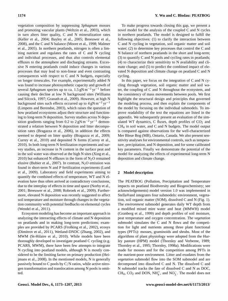
Geosci. Model Dev., 6, 1173–1207, 2013www.geosci-model-dev.net/6/1173/2013/doi:10.5194/gmd-6-1173-2013© Author(s) 2013. CC Attribution 3.0 License.
EGU Journal Logos (RGB)
Advances in Geosciences
Open A
ccess
Natural Hazards and Earth System
Sciences
Open A
ccess
Annales Geophysicae
Open A
ccess
Nonlinear Processes in Geophysics
Open A
ccess
Atmospheric Chemistry
and Physics
Open A
ccess
Atmospheric Chemistry
and Physics
Open A
ccess
Discussions
Atmospheric Measurement
Techniques
Open A
ccess
Atmospheric Measurement
Techniques
Open A
ccess
Discussions
Biogeosciences
Open A
ccess
Open A
ccess
BiogeosciencesDiscussions
Climate of the Past
Open A
ccess
Open A
ccess
Climate of the Past
Discussions
Earth System Dynamics
Open A
ccess
Open A
ccess
Earth System Dynamics
Discussions
GeoscientificInstrumentation
Methods andData Systems
Open A
ccess
GeoscientificInstrumentation
Methods andData Systems
Open A
ccess
Discussions
GeoscientificModel Development
Open A
ccess
Open A
ccess
GeoscientificModel Development
Discussions
Hydrology and Earth System
Sciences
Open A
ccess
Hydrology and Earth System
Sciences
Open A
ccess
Discussions
Ocean Science
Open A
ccess
Open A
ccess
Ocean ScienceDiscussions
Solid Earth
Open A
ccess
Open A
ccess
Solid EarthDiscussions
The Cryosphere
Open A
ccess
Open A
ccess
The CryosphereDiscussions
Natural Hazards and Earth System
Sciences
Open A
ccess
Discussions
PEATBOG: a biogeochemical model for analyzing coupled carbonand nitrogen dynamics in northern peatlands
Y. Wu and C. Blodau
Hydrology Group, Institute of Landscape Ecology, FB 14 Geosciences, University of Munster, Germany, Heisenbergstrasse 2,48149 Munster, Germany
Correspondence to:C. Blodau ([email protected])
Received: 14 November 2012 – Published in Geosci. Model Dev. Discuss.: 4 March 2013Revised: 26 May 2013 – Accepted: 26 June 2013 – Published: 9 August 2013
Abstract. Elevated nitrogen deposition and climate changealter the vegetation communities and carbon (C) and nitro-gen (N) cycling in peatlands. To address this issue we devel-oped a new process-oriented biogeochemical model (PEAT-BOG) for analyzing coupled carbon and nitrogen dynamicsin northern peatlands. The model consists of four submodels,which simulate: (1) daily water table depth and depth profilesof soil moisture, temperature and oxygen levels; (2) competi-tion among three plants functional types (PFTs), productionand litter production of plants; (3) decomposition of peat;and (4) production, consumption, diffusion and export of dis-solved C and N species in soil water. The model is novelin the integration of the C and N cycles, the explicit spa-tial resolution belowground, the consistent conceptualizationof movement of water and solutes, the incorporation of stoi-chiometric controls on elemental fluxes and a consistent con-ceptualization of C and N reactivity in vegetation and soilorganic matter. The model was evaluated for the Mer BleueBog, near Ottawa, Ontario, with regards to simulation of soilmoisture and temperature and the most important processesin the C and N cycles. Model sensitivity was tested for nitro-gen input, precipitation, and temperature, and the choices ofthe most uncertain parameters were justified. A simulation ofnitrogen deposition over 40 yr demonstrates the advantagesof the PEATBOG model in tracking biogeochemical effectsand vegetation change in the ecosystem.
1 Introduction
Peatlands represent the largest terrestrial soil C pool anda significant N pool. Globally, peat stores 547 PgC (Yu etal., 2010) and 8 to 15 PgN, accounting for one-third of theterrestrial C and 9 % to 16 % of the soil organic N stor-age (Wieder and Vitt, 2006). Northern peatlands have ac-cumulated 16 to 23 gC m−2 yr−1 throughout the Holoceneand 0.42 gN m−2 yr−1 in the past 1000 yr on average (Vittet al., 2000; Turunen et al., 2002; Limpens et al., 2006; vanBellen et al., 2011a, b). Carbon accumulation in peats hasbeen primarily attributed to low decomposition rates, whichcompensate for the low production in comparison to otherecosystems (Coulson and Butterfield, 1978; Clymo, 1984).The two characteristic environmental conditions in northernpeatlands’ high water table (WT) and low temperature, playan essential role in preserving the large C pool by impedingmaterial translocation and transformation in the permanentlysaturated zone (Clymo, 1984) Although the total N storagein peat is substantial, the scarcity of biologically availableN induces a conservative manner of N cycling in peatlands(Rosswall and Granhall, 1980; Urban et al., 1988).Sphag-nummosses are highly adapted to the nutrient-poor environ-ment and successfully compete with vascular plants througha series of competition strategies, such as inception of N thatis deposited from the atmosphere, internal recycling of N,and a minimized N release from litter with low decompos-ability (Damman, 1988; Aldous, 2002).
Climate change and elevated N deposition are likely toalter the structure and functioning of peatlands through in-teractive ways that are incompletely understood. In general,drought and a warmer environment were found to affect
Published by Copernicus Publications on behalf of the European Geosciences Union.
1174 Y. Wu and C. Blodau: PEATBOG
vegetation composition by suppressingSphagnummossesand promoting vascular plants (Weltzin et al., 2003), whichin turn alters litter quality, C and N mineralization rates(Keller et al., 2004; Bayley et al., 2005; Breeuwer et al.,2008), and the C and N balance (Moore et al., 1998; Malmeret al., 2005). In northern peatlands, nitrogen is often a lim-iting nutrient and regulates the rates of C and N cyclingand individual processes, and thus also controls elementaleffluxes to the atmosphere and discharging streams. Exces-sive N entering peatlands could induce changes in variousprocesses that may lead to non-linear and even contrastingconsequences with respect to C and N budgets, especiallyon longer timescales. For example, experimentally added Nwas found to increase photosynthetic capacity and growth ofseveralSphagnumspecies up to ca. 1.5 gN m−2 yr−1 beforecausing their decline at low N background sites (Williamsand Silcock, 1997; Granath et al., 2009). However, at high Nbackground sites such effects occurred up to 4 gN m−2 yr−1
(Limpens and Berendse, 2003), which raises the question ofhow peatland ecosystems adjust their structure and function-ing to long-term N deposition. Survey studies across N depo-sition gradients ranging from 0.2 to 2 gN m−2 yr−1 demon-strated a relation between N deposition and litter decompo-sition rates (Bragazza et al., 2006), in addition the effectsseemed to depend on litter quality (Bragazza et al., 2009;Currey et al., 2010) and deposited N forms (Currey et al.,2010). In both long-term N fertilization experiments and sur-vey studies, an increase in N content in the surface peat andin the soil water was observed at the high N sites (Xing et al.,2010) but enhanced N effluxes in the form of N2O remainedelusive (Bubier et al., 2007). In contrast, N2O emission wasfound in short-term N and P fertilization experiments (Lundet al., 2009). Laboratory and field experiments aiming toquantify the combined effects of temperature, WT and N el-evation have thus often arrived at contradictory conclusions,due to the interplay of effects in time and space (Norby et al.,2001; Breeuwer et al., 2008; Robroek et al., 2009). Further-more, elevated N deposition was recently suggested to affectsoil temperature and moisture through changes in the vegeta-tion community with potential feedbacks on elemental cycles(Wendel et al., 2011).
Ecosystem modeling has become an important approach inanalyzing the interacting effects of climate and N depositionon peatlands and in making long-term predictions; exam-ples are provided by PCARS (Frolking et al., 2002), ecosys(Dimitrov et al., 2011), Wetland-DNDC (Zhang, 2002), andMWM (St-Hilaire et al., 2010). While models have beenthoroughly developed to investigate peatland C cycling (e.g.PCARS, MWM), there have been few attempts to integrateN cycling into peatland models, although N is mostly con-sidered to be the limiting factor on primary production (Hei-jmans et al., 2008). In the mentioned models, N is generallypassively bound to C pools by C/N ratios, while active nitro-gen transformation and translocation among N pools is omit-ted.
To make progress towards closing this gap, we present anovel model for the analysis of the coupled C and N cyclesin northern peatlands. The model is designed to fulfill thefollowing objectives: (1) to clarify the interaction betweenC and N cycling in vegetation, soil organic matter and soilwater; (2) to determine key processes that control the C andN balance of northern peatlands in the short and long-term;(3) to quantify C and N pools and cycling rates in peatlands;(4) to characterize their sensitivity to N availability and cli-mate change; and (5) to predict the combined impact of ele-vated N deposition and climate change on peatland C and Ncycling.
In this paper, we focus on the integration of C and N cy-cling through vegetation, soil organic matter and soil wa-ter, the coupling of C and N throughout the ecosystem, andthe consistency of mass movements between pools. We firsthighlight the structural design and principles that governedthe modeling process, and then explain the components ofthe model by focusing on the individual submodels. To im-prove readability of the text the equations are listed in theappendix. We subsequently present an evaluation of the sim-ulated WT dynamics, C fluxes, depth profiles of CO2 andCH4 in soil water, and C and N budgets. The model outputis compared against observations for the well-characterizedMer Bleue Bog (MB), Ontario, Canada. We also present sen-sitivity analyses for environmental controls, such as tempera-ture, precipitation, and N deposition, and for some calibratedkey parameters. Finally we demonstrate the potential of themodel for analyzing the effects of experimental long-term Ndeposition and climate change.
2 Model description
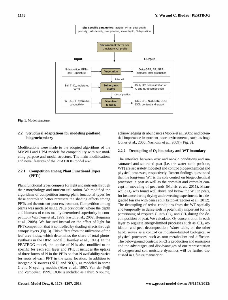
The PEATBOG (Pollution, Precipitation and Temperatureimpacts on peatland Biodiversity and Biogeochemistry; seeacknowledgements) model version 1.0 was implemented inStella®and integrates four submodels: environment, vegeta-tion, soil organic matter (SOM), dissolved C and N (Fig. 1).The environmentsubmodel generates daily WT depth froma modified mixed mire water and heat (MMWH) model(Granberg et al., 1999) and depth profiles of soil moisture,peat temperature and oxygen concentration. Thevegetationsubmodel simulates the C and N flows and the competi-tion for light and nutrients among three plant functionaltypes (PFTs): mosses, graminoids and shrubs. Most of thealgorithms of plant physiology were adopted from the Hur-ley pasture (HPM) model (Thornley and Verberne, 1989;Thornley et al., 1995; Thornley, 1998a). Modifications weremade for mosses and for the competition among PFTs inthe nutrient-poor environment. Litter and exudates from thevegetationsubmodel flow into the SOM submodel and aredecomposed into dissolved C and N. The dissolved C andN submodel tracks the fate of dissolved C and N as DOC,CH4, CO2 and DON, NH+
4 , and NO−
3 . The model does not
Geosci. Model Dev., 6, 1173–1207, 2013 www.geosci-model-dev.net/6/1173/2013/

Y. Wu and C. Blodau: PEATBOG 1175
consider hummock-hollow microtopography of peatlands,which in other studies had no statistically significant effectwhen simulating ecosystem level CO2 exchange (Wu et al.,2011).
2.1 Model structure and principles
The following three principles were imbedded in the modelin terms of scale, resolution and structure:
2.1.1 High spatial and moderate temporal resolution
In comparison to other biogeochemical process models ofpeatland C cycling (Frolking et al., 2002; St-Hilaire et al.,2010) that primarily focus on the ecosystem-atmosphere in-teractions, we increased the vertical spatial representationand kept the temporal resolution fairly low. We divided thebelowground peat into 20 layers (i) with a vertical resolutionof 5 cm except for an unconfined bottom layer. This structureapplies to all belowground pools and processes. The ratio-nale for the comparatively fine spatial resolution lies in thecritical role of soil hydrology for the C and N cycles andthe necessity to represent physical and microbial processes(Trumbore and Harden, 1997). Spatial distributions of wa-ter and dissolved chemical species are generated and massmovement and balances are examined throughout layers andpools, which allows for tracing the fate of C and N below-ground. The high resolution allows to explicitly include theactivity of plant roots and their local impact on C and Npools. Plant roots showed morphological changes upon WTfluctuation and nutrient input in bogs (Murphy et al., 2009;Murphy and Moore, 2010). Root litter also provides highlydecomposable organic matter to deeper peat and serves as asubstrate for microbial respiration. Moreover, roots can actas sensitive conductors of N deposition to deep peat via rootchemistry and litter quality (Bubier et al., 2011; Bragazzaet al., 2012). The layered structure assists in mapping thebelowground micro-environment for simulating the sensi-tive interactions of soil moisture, roots and microbial activ-ity. The model computes and simulates processes on a dailytime step, as does for example the HPM model (Thornley etal., 1995) and the wetland-DNDC model (Zhang, 2002). Themoderate temporal resolution is adequate for the model soilC in the short- and long term (Trettin et al., 2001).
2.1.2 Stoichiometry controls C and N cycles
We did not stipulate critical mass fluxes as constraints on Cand N cycling. Instead these constraints are generated in themodel from changes in biological stoichiometry. This struc-ture has the advantage that the interactions between C and Nfluxes and temporal and spatial changes in pools sizes controlthe mobility of the elements. As in some terrestrial C and Nmodels (Zhang et al., 2005), N flows are driven by C/N ratiogradients from low C/N ratio to high C/N ratio compart-ments. The C/N ratios of all pools are in turn modified by
their associated flows, reflecting the organisms’ requirementto maintain their chemical composition in certain ranges. Re-sults from field manipulation experiments suggested thresh-olds of the N deposition level, above which theSphagnummoss filter fails and mineral N enters soil water (Lamers etal., 2001; Bragazza et al., 2004). Flux-based critical loadsof N for Sphagnummoss were suggested as the high end oftheSphagnumtolerance range, where the values are between0.6 gN m−2 yr−1 (Nordin et al., 2005) and 1.5 gN m−2 yr−1
(Vitt et al., 2003). Threshold values in stoichiometry termsappear to be less variable, ranging from 15 mgN g−1 (VanDer Heijden et al., 2001; Xing et al., 2010) to 20 mgN g−1
dry mass (Berendse et al., 2001; Granath et al., 2009). Thecritical load of ca. 1 gN m−2 yr−1 was linked to a stoichiom-etry thresholds of 30 (N/P ratio) and 3 (N/K ratio) in Sphag-num mosses(Bragazza et al., 2004). The model internallygenerates C/N ratios, or C/N/P ratios, for all compartmentsto control the N flows in plants and microorganisms.
2.1.3 Consistent conceptualization of carbon andnitrogen reactivity
Differences in the mobility of C and N compartmentswere implemented using a two-pool concept throughout themodel. Similar to decomposition models that distinguish thequality of soil organic matter (Grant et al., 1993; Parton etal., 1993), C and N are presented in labile (L) and recalci-trant (R) pools in SOM. In addition, the model differentiatedC and N pools based on quality in vegetation, into structural(struc) pools (Fig. 2). The pasture vegetation model HPM(Thornley et al., 1995; Thornley, 1998b) was adopted, whereC and N in grass and legumes were separated in structuraland substrate pools in shoots (sh) and roots (rt) for 4 agecategories. Considering our focus on competition betweenplant functional types, vegetation was not conceptualized interms of age categories but instead classified into 3 plantfunctional types (PFTs) (j : 1= mosses, 2= graminoids and3= shrubs) that are characterized by distinctive ecologicalfunctions (Fig. 3) in our model. The plant functional typesdiffer in the decomposability of the litter, which was repre-sented by the different mass fractions of the labile carbonpool in the litter. The fraction of labile litter was assumedto be 0.1, 0.3 and 0.2 in mosses, graminoids and shrubs, re-spectively (Inglett et al., 2012). Once the litter is depositedthe litter merges into one labile and one recalcitrant soil or-ganic matter pool. The remaining fraction of the plant litteris assigned to be recalcitrant and represents the input into therecalcitrant soil organic matter pools. Thus, the compositionof plants, as a result of net primary production and litter fall,is adjusted to physical conditions and N input and alters SOMquality via changes in litter quality (Q).
www.geosci-model-dev.net/6/1173/2013/ Geosci. Model Dev., 6, 1173–1207, 2013
1176 Y. Wu and C. Blodau: PEATBOG
1
Figure 1. Model structure
Environment: WTD, soil
T, moisture, O2 profile
Hydraulic conductivity
Vegetation
Soil organic
matter
Dissolved
C and N
CO2, CH4, N2O, DIN, DOC,
DON content and export
WT, O2, T, hydraulic
conductivity
Soil T, O2, moisture,
WTD
N deposition, PFTs,
soil T, moisture
Daily GPP, AR, NPP,
biomass, litter production
Daily HR, sequestration of
C and N, decomposition
Output Input
Site specific parameters: latitude, PFTs, peat depth,
porosity, bulk density, precipitation, snow depth, N deposition
Litterfall
Decomposition
Fig. 1.Model structure.
2.2 Structural adaptations for modeling peatlandbiogeochemistry
Modifications were made to the adopted algorithms of theMMWH and HPM models for compatibility with our mod-eling purpose and model structure. The main modificationsand novel features of the PEATBOG model are:
2.2.1 Competition among Plant Functional Types(PFTs)
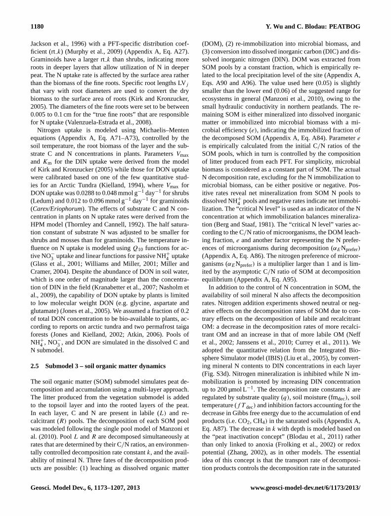
Plant functional types compete for light and nutrients throughtheir morphology and nutrient utilization. We modified thealgorithms of competition among plant functional types forthese controls to better represent the shading effects amongPFTs and the nutrient-poor environment. Competition amongplants was modeled using PFTs previously, where the depthand biomass of roots mainly determined superiority in com-petition (Van Oene et al., 1999; Pastor et al., 2002; Heijmanset al., 2008). We focused instead on the effect of light forPFT competition that is controlled by shading effects throughcanopy layers (Fig. 3). This differs from the utilization of theleaf area index, which determines the share of total photo-synthesis in the HPM model (Thornley et al., 1995). In thePEATBOG model, the uptake of N is also modified to bespecific for each soil layer and PFT. It includes the uptakeof three forms of N in the PFTs so that N availability variesfor roots of each PFT in the same location. In addition toinorganic N sources (NH+4 and NO−
3 ), as modeled in someC and N cycling models (Aber et al., 1997; Van der Peijland Verhoeven, 1999), DON is included as a third N source,
acknowledging its abundance (Moore et al., 2005) and poten-tial importance in nutrient-poor environments, such as bogs(Jones et al., 2005; Nasholm et al., 2009) (Fig. 3).
2.2.2 Decoupling of O2 boundary and WT boundary
The interface between oxic and anoxic conditions and un-saturated and saturated peat (i.e. the water table position,WT) are separately modeled and control biogeochemical andphysical processes, respectively. Recent findings questionedthat the long-term WT is the sole control on biogeochemicalprocesses in peat as well as theacrotelmandcatotelmcon-cept in modeling of peatlands (Morris et al., 2011). Mean-while O2 was found well above and below the WT in peats,for instance during drying and rewetting experiments in a de-graded fen site with dense soil (Estop-Aragones et al., 2012).The decoupling of redox conditions from the WT spatiallyand temporally in dense soils is potentially important for thepartitioning of respired C into CO2 and CH4during the de-composition of peat. We calculated O2 concentration in eachlayer to regulate energy-limited processes such as CH4 ox-idation and peat decomposition. Water table, on the otherhand, serves as a control on moisture-limited biological orphysical processes, such as root metabolism and diffusion.The belowground controls on CH4 production and emissionsand the advantages and disadvantages of our representationof oxygen and soil moisture dynamics will be further dis-cussed in a future manuscript.
Geosci. Model Dev., 6, 1173–1207, 2013 www.geosci-model-dev.net/6/1173/2013/

Y. Wu and C. Blodau: PEATBOG 1177Change in Figures
Please change Fig. 2 to the following:
Den
itrifica
tion
(Eq
. A1
57
-A1
62
)
N deposition
CO
2 pro
ductio
n
(Eq
.A1
11
)
CH
4 pro
ductio
n
(Eq
. A1
14
)
Exu
da
tion N
Exu
da
tion C
Pla
nt T
ran
sp
ort
SO4 reduction
(Eq. A129)
Humic Substances
Eb
ullitio
n
(Eq
. A1
19
)
Shoot
Substrate C
Peat Labile C
Shoot
Structural C
Shoot
Substrate N
Shoot
Structural N
Peat
Recalcitrant C Peat Labile N Peat
Recalcitrant N
NH4+
NO3-
Root
Substrate C
Root
Structural C
Root
Substrate N
Root
Structural N
Uptake
(Eq. A71)
N2 fix
atio
n
(Eq
. A1
47
)
Electron
acceptors
Deco
mp
ositio
n
(Eq
. A9
3, A
99
)
Oxidation
(Eq. A117) DIC CH4
Litte
r
(Eq
.A3
4-
A3
6, A
55
)
Run
off
(Eq
. A1
63
)
Diffu
sio
n
(Eq
. A1
06
)
Resp
iratio
n
PS
N
Nitrification
(Eq. A151)
Eq. A51
Eq. A51
Eq. A58 Eq. A58
Eq
. A3
8
Eq
. A4
9, A
54
Eq
. A6
0
Eq
. A6
9
Eq. A67
Eq. A67
DON
(Eq
. A1
15
)
(Eq. A143)
(Eq. A122)
DOC
Fig. 2.Schematic C N pools and flows. The black lines are material flows and the dotted lines are information flows. Equations are equationsas listed in Appendix A.
2.3 Submodel 1 – environmental controls
Physical boundary conditions, such as day length, degreedays, water table depth, soil moisture, temperature and depthprofiles of O2, are generated by the model to control physio-chemical and biological processes.
Day length (DL), which in the model controls photosyn-thesis, varies for geographic position of the site and day ofyear. The daily day length value is obtained from the anglebetween the setting sun and the south point, which in turnis calculated from the declination of the earth and the ge-ographical position of the site (Brock, 1981) (Appendix A,Eqs. A14 and A15). Declination of the earth is the angulardistance at solar noon between the sun and the equator andpositive for the Northern Hemisphere. The value of declina-tion is approximately calculated by Cooper (1969) using theday of the year.
Temperature is modeled by sinusoidal equations (Carslawand Jaeger, 1959) and modified by converting a dampen-ing depth into thermal conductivity (Appendix A, Eq. A13).Thermal conductivity (Kthermal) is adjusted for each layer forpeat compaction and snow coverage that delays the thermalexchange in winter and early spring (Fig. S1a, Supplement).
Degree days (DD) represent the accumulation of cold daysand trigger defoliation (Frolking et al., 2002; Zhang, 2002).Similar to other models, defoliation occurs on the day whenDD reaches minus 25 degrees, with accumulated temperatureof lower than 0 degrees after day 181 of the year (1 July innon-leap years).
Water table (WT) depth is simulated by calculating the wa-ter table depth from the water storage of peat using a modi-fied version of the Mixed Water and Heat model (MMWH)(Granberg et al., 1999). Precipitation and snowmelt repre-sent water inputs, and are obtained from local meteorological
www.geosci-model-dev.net/6/1173/2013/ Geosci. Model Dev., 6, 1173–1207, 2013

1178 Y. Wu and C. Blodau: PEATBOG
3
Figure 3. Plant competition for nutrient and light
De
cre
asin
g lig
ht
De
po
site
d N
Graminoids Canopy
Shrubs Canopy
Mosses Canopy
Gra
min
oid
s R
oo
ts
Sh
rub
s ro
ots
DON
DIN
De
cre
asin
g D
IN
Peat
Fig. 3.Plant competition for nutrient and light.
records, instead of modeling the snow cover. Evapotranspi-ration (EPT) is the water output from the peat and vegetationsurface via evaporation and transpiration, which are regu-lated by temperature and vegetation characteristics. Differentfrom the authors’ original approach, the EPT rate per unit ofthe peatland surface is calculated from a base EPT rate andmultipliers of plant leaf area (Reimer, 2001) (Appendix A,Eq. A3), daily air temperature (Fig. S1b), daily average pho-tosynthetic active radiation (PAR), and a factor of WTD androoting depth (Lafleur et al., 2005a) (Fig. S2c). A maximumwater storage was added to allow overflow once the WTrises above the peat surface. WTD is then obtained from lin-ear functions of water storage as in the MMWH model butwith depth-dependent slopes (Appendix A, Eq. A8). The WTlayer is defined as the layer in which the WT is located.
Depth profiles of soil moisture (m3 water m−3 pore space)are generated by the Van Genuchten’s soil water retentionequation, parameterized by Letts et al. (2000) for peatlands(Appendix A, Eq. A9). Porosity is a function of depth derivedfrom field measurements for the Mer Bleue Bog (Blodau andMoore, 2002).
In order to simulate exports of dissolved C and N withoutmodeling water movement explicitly, runoff was distributedover 20 layers and divided into horizontal and vertical flows(Fig. 4, Appendix A, Eq. A4–A7). The vertical advection ratedepends on slope and is determined as a fraction of the totalrunoff. It is consistently applied to all layers. The remainingrunoff is horizontally distributed among layers according tothe vertical hydraulic conductivity distribution. In the MerBleue Bog, saturated hydraulic conductivity rapidly declineswith depth in the acrotelm, ranging from 10−7 to 10−3 m s−1
and reaching 10−8 to 10−6 m s−1 in the catotelm (Fraser etal., 2001b). In layers above the WT, the actual hydraulic
4
Figure 4. Schematic soil water flow
PRE = precipitation
EPT = evapotranspiration
Runoff from each layer varies according to hydraulic conductivity
PR
E
Peat Layers
EP
T
Water table
Advectio
n
Fig. 4.Schematic soil water flow.
conductivity is lower when pores are unsaturated (Hemondand Fechner-Levy, 2000) (Fig. S1d).
The depth profiles of O2 concentrations are simulated tolocate the oxic-anoxic interface. Oxygen diffuses from thesurface to deeper soil layers and is consumed directly or in-directly by the oxidization of peat C to CO2 (Appendix A,Eq. A12). For the simulation of oxygen-dependent biogeo-chemical processes we chose a dichotomous distribution ofO2, where the boundary of oxic/anoxic conditions is set at5 µmol L−1 (Liou et al., 2008).
2.4 Submodel 2 – vegetation
Carbon in vascular plants is represented by four pools: shootsubstrate C (shsubsC), root substrate C (rtsubsC), shootstructural C (shstrucC), and root substrate C (rtsubsC)(Fig. 2). Substrate C and structural C refer to metabolic ac-tivated C and recalcitrant C, respectively. Substrate poolsconduct metabolic activities (i.e. photosynthesis, respira-tion) and structural pools perform phenological activities (i.e.growth, litter production). The flow from substrate C to struc-tural C leads to plant growth (Appendix A, Eq. A33). EachC pool or flow is bound to an N pool or flow by the C/N ra-tio of the specific pool. Furthermore, shoots are divided intostems and leaves and roots into coarse and fine roots by ratiosspecific to the PFT. Mosses are represented by 4 abovegroundpools and two compartments:capitulumand stem. The C andN contained in exudates are transferred from the vegetationinto the uppermost labile C and N pools in the soil. UnlikeN uptake by vascular plants from soil water, N uptake bymosses is restricted to atmospheric supply.
Most C and N material flows are driven by C concentra-tion gradients except for a few processes controlled by N
Geosci. Model Dev., 6, 1173–1207, 2013 www.geosci-model-dev.net/6/1173/2013/

Y. Wu and C. Blodau: PEATBOG 1179
(i.e. N uptake, N recycling from litter production). The phe-nology and competing strategies of PFTs are modeled as fol-lows: (1) considering the seasonal C and N loss in leaves ofdeciduous shrubs; (2) PFT-specific N flows during growth,recycling and litter production; (3) competition among PFTis implemented through shading effects, tolerance to mois-ture and temperature, distribution of C and N among shootsand roots, as well as turnover rates. In general, the photo-synthetic nutrient-use efficiency (the ratio of photosynthesisrate and nitrogen content per leaf area) is higher in herba-ceous than in evergreen woody species (Hikosaka, 2004).The growth rates in deciduous species (graminoids and de-ciduous shrubs) are higher than in evergreen shrubs, which inturn is higher than in mosses (Chapin III and Shaver, 1989).Graminoids are more competitive in the deep soil attributedto the longer roots (Murphy et al., 2009). Mosses have theadvantage of aboveground N uptake and filtration. Below wediscuss the modeling of these competition strategies.
2.4.1 Photosynthesis (PSN) and competition for light
Competition for PAR is implemented through shading ef-fects. The light level that reaches a specific PFT after in-terception by a taller PFT determines the C assimilation ofthis PFT (Fig. 3). For each PFT, canopy PSN is integratedfrom daily leaf PSN by a light attenuation coefficient (kext),leaf area index (LAI) and day length (DL) (Appendix A,Eq. A38). The coefficientkext is unitless, the values are0.5 for graminoids (Heijmans et al., 2008), 0.97 for shrubs(Aubin et al., 2000), and assumed to be 0.9 for mosses. LAIis determined by leaf structural C mass and specific leaf area(SLA) of the PFT. The PSN rate for the top canopy layerof each PFT (LeafPSNj ) is calculated by a non-rectangularhyperbola (Fig. S2f, Appendix A, Eq. A40). The two param-etersαj andξ control the shape of the hyperbola curves. Pa-rameterαj represents the photosynthetic efficiency, which iscontrolled by WT depth, the air temperature (Tair) and at-mospheric CO2 level (CO2,air) (Appendix A, Eq. A42). Thespring PSN of mosses starts when the snow depth falls below0.2 cm. The variable LIj is the PAR incepted by the canopyof PFTj (umol m−2 s−1). The assumptions here were that ra-diation diminishes along with canopy depth and each canopydepth contains one PFT solely.
The asymptote of leaf photosynthesis rate (Pmax ingCO2 m−2 s−1) is regulated byTair, CO2,air, WT depth, Ncontent in plant shoots and the season. The maximum PSNrate (Pmax,20, g CO2 m−2 s−1) occurs in an optimal environ-ment, is also referred to as PSN capacity, and is often de-rived from measurements. The values ofPmax,20 vary amongand within growth forms and follow the general sequenceof deciduous> evergreens> mosses (Chapin III and Shaver,1989; Ellsworth et al., 2004). The maximum PSN ratePmax,20 is 0.002 g CO2 m−2 s−1 for graminoids and mossesfollowing HPM (Thornley, 1998a), and 0.005 g CO2 m−2 s−1
for shrubs based on the ranges in Small (1972). The
temperature dependence(fT ,P max,j ) of Pmax is conceptual-ized as sigmoidal curve with PFT-specific optimal, maximumand minimum temperature for photosynthesis and curvatureq (Fig. S2e, Appendix A, Eq. A43). The WT depth depen-dency ofPmax (fm,P max,j ) for mosses follows Frolking etal. (2002) and is an exponential function with PFT-specificbase (aw,j ) for vascular plants (Fig. S2a and b). The modelconsiders season and nutrient availability effects onPmax.Seasonal change (fseason,P max) affects mosses alone between0 to 1 and was derived from the maximum rates of carboxy-lation (Vmax) in spring summer and autumn (Williams andFlanagan, 1998) (Fig. S2c).
Potential N stress on photosynthesis is modeled by us-ing PFT-specific photosynthetic N use efficiencies. Althoughthere are interacting controls on the N economy of plantphotosynthesis, such as N effects on Rubisco activity, Ru-bisco regeneration and the distribution of N in leaves, thereseems to be a generalized linear relation of foliar N con-tent and PSN capacity across growth forms and seasons(Sage and Pearcy, 1987; Reich et al., 1995; Yasumura etal., 2006). The ratio of PSN capacity and foliar N concen-tration is defined as photosynthetic nitrogen use efficiency(PNUE) (Field and Mooney, 1986). In general, evergreenshave lower PNUE and larger interception than the decid-uous shrubs (Fig. S2d, Appendix A, Eq. A47) (Hikosaka,2004). To reflect N use strategies of growth forms, we im-plemented PNUE values for PFTs following the sequence:graminoids> shrubs> mosses, and interception values re-versely. In addition, a toxic effect (fN,toxic) is applied withregard to mosses when the substrate N concentration exceedsthe maximum N concentration at 20 mg g−1 (Granath et al.,2009).
2.4.2 Competition for nutrients
PFTs compete for N through two processes: filtration of de-posited N by mosses and the uptake of N among vascularplants roots. Nitrogen deposited from the atmosphere is firstabsorbed by moss and then enters soil water to become avail-able to vascular plants. The N/P ratio of mosses is used as aregulator of N pathways and an indicator of N saturation inmosses. A fraction of 95 % of the deposited N is absorbed bymoss until the N/P ratio reaches 15 (Aerts et al., 1992), abovewhich N absorption decreases owing to the co-limitation ofN and P on PSN rates. We assume mosses become N satu-rated when the N/P ratio exceeds 30 (Bragazza et al., 2004),above which the uptake fraction declines to zero. Due to thelack of P pools in the current model version, the initial mossN/P ratio is assumed to be 10 in mosses (Jauhiainen et al.,1998).
The competition for uptake of N among PFTs is conductedthrough the competitive advantages in the architecture of theroots and capabilities for uptake of three N sources (NH−
4 ,NO−
3 and DON) (Fig. 3).The root distribution in soil is mod-eled using a asymptotic equation (Gale and Grigal, 1987;
www.geosci-model-dev.net/6/1173/2013/ Geosci. Model Dev., 6, 1173–1207, 2013
1180 Y. Wu and C. Blodau: PEATBOG
Jackson et al., 1996) with a PFT-specific distribution coef-ficient (rt k) (Murphy et al., 2009) (Appendix A, Eq. A27).Graminoids have a larger rtk than shrubs, indicating moreroots in deeper layers that allow utilization of N in deeperpeat. The N uptake rate is affected by the surface area ratherthan the biomass of the fine roots. Specific root lengths LVj
that vary with root diameters are used to convert the drybiomass to the surface area of roots (Kirk and Kronzucker,2005). The diameters of the fine roots were set to be between0.005 to 0.1 cm for the “true fine roots” that are responsiblefor N uptake (Valenzuela-Estrada et al., 2008).
Nitrogen uptake is modeled using Michaelis–Mentenequations (Appendix A, Eq. A71–A73), controlled by thesoil temperature, the root biomass of the layer and the sub-strate C and N concentrations in plants. ParametersVmaxand Km for the DIN uptake were derived from the modelof Kirk and Kronzucker (2005) while those for DON uptakewere calibrated based on one of the few quantitative stud-ies for an Arctic Tundra (Kielland, 1994), whereVmax forDON uptake was 0.0288 to 0.048 mmol g−1 day−1 for shrubs(Ledum) and 0.012 to 0.096 mmol g−1 day−1 for graminoids(Carex/Eriophorum). The effects of substrate C and N con-centration in plants on N uptake rates were derived from theHPM model (Thornley and Cannell, 1992). The half satura-tion constant of substrate N was adjusted to be smaller forshrubs and mosses than for graminoids. The temperature in-fluence on N uptake is modeled usingQ10 functions for ac-tive NO−
3 uptake and linear functions for passive NH+
4 uptake(Glass et al., 2001; Williams and Miller, 2001; Miller andCramer, 2004). Despite the abundance of DON in soil water,which is one order of magnitude larger than the concentra-tion of DIN in the field (Kranabetter et al., 2007; Nasholm etal., 2009), the capability of DON uptake by plants is limitedto low molecular weight DON (e.g. glycine, aspartate andglutamate) (Jones et al., 2005). We assumed a fraction of 0.2of total DON concentration to be bio-available to plants, ac-cording to reports on arctic tundra and two permafrost taigaforests (Jones and Kielland, 2002; Atkin, 2006). Pools ofNH+
4 , NO−
3 , and DON are simulated in the dissolved C andN submodel.
2.5 Submodel 3 – soil organic matter dynamics
The soil organic matter (SOM) submodel simulates peat de-composition and accumulation using a multi-layer approach.The litter produced from the vegetation submodel is addedto the topsoil layer and into the rooted layers of the peat.In each layer, C and N are present in labile (L) and re-calcitrant (R) pools. The decomposition of each SOM poolwas modeled following the single pool model of Manzoni etal. (2010). PoolL andR are decomposed simultaneously atrates that are determined by their C/N ratios, an environmen-tally controlled decomposition rate constantk, and the avail-ability of mineral N. Three fates of the decomposition prod-ucts are possible: (1) leaching as dissolved organic matter
(DOM), (2) re-immobilization into microbial biomass, and(3) conversion into dissolved inorganic carbon (DIC) and dis-solved inorganic nitrogen (DIN). DOM was extracted fromSOM pools by a constant fraction, which is empirically re-lated to the local precipitation level of the site (Appendix A,Eqs. A90 and A96). The value used here (0.05) is slightlysmaller than the lower end (0.06) of the suggested range forecosystems in general (Manzoni et al., 2010), owing to thesmall hydraulic conductivity in northern peatlands. The re-maining SOM is either mineralized into dissolved inorganicmatter or immobilized into microbial biomass with a mi-crobial efficiency (e), indicating the immobilized fraction ofthe decomposed SOM (Appendix A, Eq. A84). Parametere
is empirically calculated from the initial C/N ratios of theSOM pools, which in turn is controlled by the compositionof litter produced from each PFT. For simplicity, microbialbiomass is considered as a constant part of SOM. The actualN decomposition rate, excluding for the N immobilization tomicrobial biomass, can be either positive or negative. Pos-itive rates reveal net mineralization from SOM N pools todissolved NH+4 pools and negative rates indicate net immobi-lization. The “critical N level” is used as an indicator of the Nconcentration at which immobilization balances mineraliza-tion (Berg and Staaf, 1981). The “critical N level” varies ac-cording to the C/N ratio of microorganisms, the DOM leach-ing fraction,e and another factor representing the N prefer-ences of microorganisms during decomposition (αENprefer)
(Appendix A, Eq. A86). The nitrogen preference of microor-ganisms (αENprefer) is a multiplier larger than 1 and is lim-ited by the asymptotic C/N ratio of SOM at decompositionequilibrium (Appendix A, Eq. A95).
In addition to the control of N concentration in SOM, theavailability of soil mineral N also affects the decompositionrates. Nitrogen addition experiments showed neutral or neg-ative effects on the decomposition rates of SOM due to con-trary effects on the decomposition of labile and recalcitrantOM: a decrease in the decomposition rates of more recalci-trant OM and an increase in that of more labile OM (Neffet al., 2002; Janssens et al., 2010; Currey et al., 2011). Weadopted the quantitative relation from the Integrated Bio-sphere Simulator model (IBIS) (Liu et al., 2005), by convert-ing mineral N contents to DIN concentrations in each layer(Fig. S3d). Nitrogen mineralization is inhibited while N im-mobilization is promoted by increasing DIN concentrationup to 200 µmol L−1. The decomposition rate constantsk areregulated by substrate quality (q), soil moisture (fmdec), soiltemperature (f T dec) and inhibition factors accounting for thedecrease in Gibbs free energy due to the accumulation of endproducts (i.e. CO2, CH4) in the saturated soils (Appendix A,Eq. A87). The decrease ink with depth is modeled based onthe “peat inactivation concept” (Blodau et al., 2011) ratherthan only linked to anoxia (Frolking et al., 2002) or redoxpotential (Zhang, 2002), as in other models. The essentialidea of this concept is that the transport rate of decomposi-tion products controls the decomposition rate in the saturated
Geosci. Model Dev., 6, 1173–1207, 2013 www.geosci-model-dev.net/6/1173/2013/

Y. Wu and C. Blodau: PEATBOG 1181
anoxic soils (Fig. S3). The inhibitions factors are values be-tween 0 and 1 based on CO2 and CH4 concentrations accord-ing to the inverse modeling results in Blodau et al. (2011)(Fig. S3a and b).
The intrinsic decomposability of the substrate (L or R) de-termines the base decomposition rate constant (kCpot). Due tothe conceptual inconsistency ofkCpot in experiments (Upde-graff et al., 1995; Bridgham et al., 1998), we calibrated thevalues ofkCpot from the long-term simulations in the spin-upruns. The moisture and temperature effect on the decompo-sition is each pool is modeled similar to the PCARS model(Frolking et al., 2002), with theQ10 value of the decompo-sition of L pools (2.3) smaller than of that ofR pools (3.3)(Conant et al., 2008, 2010).
2.6 Submodel 4 – dissolved C and N
The model contains 3 dissolved C pools: CH4, CO2 and DOCand 4 dissolved N pools: NH+4 , NO−
3 , NO−
2 and DON in eachbelowground layer (Fig. 2). Because decomposition proceedsand is controlled through the SOM pools, DOC and DON areconsidered to be an end product, and are only removed byrunoff. The production of DOC, DIC, DON and NH+4 are in-puts from the SOM and the vegetation submodels. The pro-duction of DIC is further partitioned into the production ofCH4 and CO2 in the anoxic layers.
The partitioning of respired C into CO2 and CH4 in thesaturated layers depends on the presence of alternative elec-tron acceptors (i.e. SO2−
4 , NO−
3 and likely humic substances)for the terminal electron accepting processes (TEAP) (Con-rad, 1999; Lovley and Coates, 2000). In previous studies,the ratio of CO2/CH4 production and the production rates ofCH4 was modeled as a function of WT depth (Potter, 1997;Zhuang, 2004), or by microbial activities using Michaelis–Menten kinetics (Segers and Kengen, 1998; Lopes et al.,2011). Following the concept put forward by Blodau (2011),we modeled the CH4 production rate by an energy-limitedMichaelis–Menten kinetics.
We built an equation group based on the valance balanceof the overall oxidation-reduction process and the mass bal-ance of C (Appendix A, Eq. A121). The first equation (Ap-pendix A, Eq. A121) denotes that CO2 and CH4 are the onlyinorganic C products (DIC) from the decomposition of SOM.The second equation was deduced from the valance balanceof CO2 (+4) production and CH4(−4) production from or-ganic C, assuming an initial oxidation state of zero as foundin carbohydrates. The production of CO2 (CO2proi) is theresult of the stoichiometric release of CH4 (CH4proi) fromfermentation and subsequent methanogenesis, and the con-sumption of electron acceptors (CO2proEA,i) in units of elec-tron equivalents. The acronym EA represents electron accep-tors other than CO2, including NO−
3 , SO2−
4 , and humic sub-stances (HS).
In anaerobic systems, electron acceptors are consumedby terminal electron accepting processes that competitively
consume H2 or acetate. Individual processes predominate ac-cording to their respective Gibbs free energy gain, usually inthe sequence NO−3 , Fe (III), humic substances (HS), SO2−
4and CO2 (Conrad, 1999; Blodau, 2011). Owing to the ex-tremely fast turnover of H2 pools in peat, the Michaelis–Menten approach is not suitable for modeling CH4 produc-tion in models running on a daily time step when H2 is con-sidered the substrate. To avoid modeling the pools of H2 andacetate explicitly, the current model with daily time step fo-cuses on the electron flow from complex organic matter to allTEAPs, instead of modeling each microbial process explic-itly. In ombrotrophic systems like bogs, only SO2−
4 , NO−
3 andHS are considered relevant electron acceptors. The CO2 pro-duction from SO2−
4 and NO−
3 reduction are calculated fromthe valance relations (Appendix A, Eq. A122), One mole ofSO2−
4 being reduced to HS− provides 8 mole of electrons(S(+6)→ S(−2)) and 1 mole of NO−3 release 5, 4 and 3moles of electrons when being reduced to NO, N2O or N2(N(+5)→ N(+3)→ N(+1)→ N(0)).
Humic substances have recently also been identified aselectron acceptors (Lovley et al., 1996; Heitmann et al.,2007; Keller et al., 2009) and require some consideration.Reduction of humic substances may be a significant CO2source in anoxic peat, where a large fraction of the total CO2production typically cannot be explained by consumption ofknown electron acceptors (Vile et al., 2003b). Although peatstores a large amount of organic carbon as humics, likelyonly a small fraction of it is redox active (Roden et al., 2010).The redox-active moieties in humics have been identified asquinones, here called DOM-Q (Scott et al., 1998). Electronaccepting rate constants of HS in sediments were reported tobe 0.34 h−1 and 0.68 h−1 based on two oxidized humic pools(Roden et al., 2010). Field measurements reported minimumelectron transfer of 0.8 mmol charge (eq.) m−2 day−1 gener-ating CO2 at 0.2 mmol m−2 day−1 (Heitmann et al., 2007).This rate was similar to the small production rate of CH4 atthe investigated bog site.
Based on this limited information, we conceptually mod-eled the reduction and oxidation of humic substances us-ing first order kinetics (Appendix A, Eqs. A133–136). Theinitial values of the EA (electron acceptors) and ED (elec-tron donors) pools in the humic substances are calculatedfrom the SOM C pool by a ratio of 1.2 eq. (mol C)−1 (Ro-den et al., 2010). The initial electron accepting capacity usedin the model was ca. 2000–4000 mmol charge m−2 for theupper 60 cm of peat per m2, which is close to the capacityof 2725 mmol charge m−2 derived from a drying and rewet-ting experiments in a minerotrophic fen (Knorr and Blodau,2009).
In the model electron acceptors are renewed via two mech-anisms: direct oxidation by O2 due to WT fluctuation in theonly temporarily saturated layers and microbially mediatedelectric currents through the peat column via an extracellu-lar electron transfer (Inanowire). While the first mechanism is
www.geosci-model-dev.net/6/1173/2013/ Geosci. Model Dev., 6, 1173–1207, 2013

1182 Y. Wu and C. Blodau: PEATBOG
well documented (Knorr and Blodau, 2009), the second isspeculative. It relates to the observation that even in deeperpeats, that are not affected by influx of oxygen or other in-organic electron acceptors, CO2 seems to be net released inexcess of methane (Beer and Blodau, 2007). This finding hasremained enigmatic because excess CO2 release would beimpossible from a stoichiometric point of view when organicmatter with oxidation state close to zero is respired and other,more reduced decomposition products, in particular molecu-lar hydrogen, are not concurrently released. A relevant accu-mulation of molecular hydrogen has, to our knowledge, notbeen observed in affected peats. Anaerobic methane oxida-tion may appear as a way out of the dilemma; however, alsothis process would depend on the elusive electron acceptor(Smemo and Yavitt, 2011).
Recently an extracellular electron transfer was describedthat has the potential to solve this enigma. Microorganismsin soils and sediments were first detected extracellularly uti-lizing electrons from redox active species, such as HS, andFe (III) (Lovley and Coates, 2000). The term “microbialnanowire” was proposed later for this extracellular electrontransfer (Reguera et al., 2005). Recently the process wasdemonstrated to occur in marine sediments over macroscopicdistances (Nielsen et al., 2010). The authors suggested thatelectrons can extracellularly flow in interconnected networksof “nanowires” so that oxidation and reduction process arespatially separated from each other. In our case the oxidationprocess releasing CO2 would proceed deeper into the peat,whereas the reduction reaction would take place near thepeatland surface where oxygen is present. We suppose thatthis mechanism may be the reason for some of the frequentlyobserved CO2 production that is unrelated to physical sup-ply of an electron acceptor deeper into the peat. Not know-ing about mechanistic detail in peats, we conceptualized thisprocess by simply calculating an extracellular electron cur-rent in the peat and using Ohm’s law for the anoxic layers(Appendix A, Eq. A137). Peat electron flow resistance (R) isdetermined by inverse modeling based on the resistance con-stant definition and corrected for soil moisture under the as-sumption that air-filled pore space cannot conduct electrons(Appendix A, Eq. A142). The parameternpeat (U m) is thespecific resistance of the material andl is the layer depth(m). Electron current in mA was then converted to mmolby the Avogadro constant (NA) and the Faraday constant(F) (96 490 Coulombs mol−1) (Appendix A, Eq. A137). Tomake this process work, electrochemical potential gradients(dEh) that drive the flow between adjacent layers are needed.In absence of meaningful measurements of redox potentialof peat we calculated such a gradient from a measured re-dox potential gradient in the Mer Bleue Bog that was givenby concentration depth profiles of dissolved H2, CO2, andCH4. We assumed that the redox potential gradient of thisredox couple represents the minimum depth gradient in elec-trochemical potentials being present. Using the Nernst equa-tion for the reaction 4H2 (aq)+ CO2 (aq)→ 2H2O (l) + CH4
(aq) (Appendix A, Eqs. A138–A141), concentration profileswere converted into electrochemical potential gradients withdepth. H2 concentration was measured by Beer and Blodaufor the Mer Bleue bog (2007) (Table S4).
In the model the electron flow through the peat towardsthe peatland surface is used to reoxidize H2S to sulfate andDOM-QH2 to DOM-Q at larger depths. These species arethe reduced again, producing the needed “excess” CO2 inthe process and lowering rates of methanogenesis, respec-tively (Appendix A, Eq. A136). The rate constant of sul-fate reduction was adjusted to the suggested range of theSO2−
4 reduction rates based on the S deposition on the siteat 0.89 mmol S m−3 day−1 (Vile, 2003a). The same thermo-dynamic inhibition concept as used to model methanogenesiswas applied also to bacterial sulfate reduction (Appendix A,Eq. A129).
Both CO2 and CH4 are in equilibrium between gaseousphase and dissolved phase obeying Henry’s Law (Ap-pendix A, Eqs. A100–A103). The efflux of C and N arethrough runoff and advection in dissolved phase and ingaseous phase from the soil surface. Diffusion follows Fick’slaw with moisture-corrected coefficients in the saturated lay-ers and was modeled as step functions in the unsaturated lay-ers where diffusion accelerates by orders of magnitude forgases (Appendix A, Eqs. A104–A107). CH4 also escapesfrom the soil via ebullition and plant-mediated transporta-tion (Appendix A, Eqs. A115–A120). Ebullition occurs insaturated layers once CH4 level exceeds the maximum con-centration CH4,max. The parameter CH4,max is sensitive totemperature and pressure (Davie et al., 2004), with a basemaximum CH4 concentration at 500 uM, which is the valuefor a vegetated site at 10◦C in Walter et al. (2001). Theebullition of CH4 releases the gas to the atmosphere with-out it passing through the unsaturated zone. In the rootedlayers, graminoids transport CH4 at rates that are deter-mined by the biomass of the graminoid roots. A percentageof 50 % of the CH4 are oxidized to CO2 during the plant-mediated transportation by the O2 in plant tissues (Walter etal., 2001). The CH4 oxidation in the oxic layers was modeledusing temperature-sensitive double Michaelis–Menten func-tions (Segers and Leffelaar, 2001) (Appendix A, Eq. A118).
The gases N2O and NO are byprod-ucts of nitrification and denitrification(NH+
4 →NO−
2 → NO−
3 → NO−
2 → NO→ N2O→ N2)
in the oxic and anoxic layers, respectively. During ni-trification, the fraction of N loss as NO (rNOnitri) is0.1 %–4 % day−1 with a mean value of 2 % (Baumgartnerand Conrad, 1992; Parsons et al., 1996). For N2O (rN2Onitri)
this value is smaller at 0.1 %–0.2 % day−1 (Ingwersen et al.,1999; Breuer et al., 2002; Khalil et al., 2004a). We usedsimilar values as in the model DNDC for acid ecosystems,where rN2Onitri was 0.06 % andrNOnitri was 0.25 % (Liand Aber, 2000). Both nitrification and denitrification areregulated by temperature, moisture, and pH. Moisture is the
Geosci. Model Dev., 6, 1173–1207, 2013 www.geosci-model-dev.net/6/1173/2013/
Y. Wu and C. Blodau: PEATBOG 1183
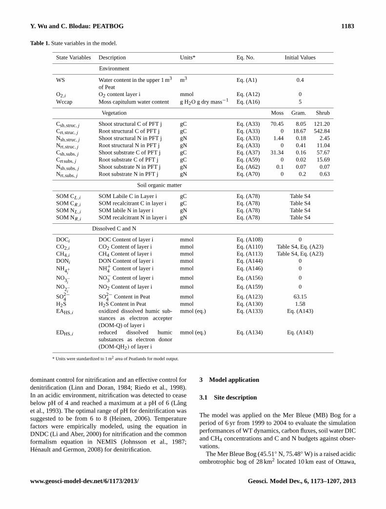
Table 1.State variables in the model.
State Variables Description Units* Eq. No. Initial Values
Environment
WS Water content in the upper 1 m3
of Peatm3 Eq. (A1) 0.4
O2,i O2 content layer i mmol Eq. (A12) 0Wccap Moss capitulum water content g H2O g dry mass−1 Eq. (A16) 5
Vegetation Moss Gram. Shrub
Csh,struc,j Shoot structural C of PFT j gC Eq. (A33) 70.45 8.05 121.20Crt,struc,j Root structural C of PFT j gC Eq. (A33) 0 18.67 542.84Nsh,struc,j Shoot structural N in PFT j gN Eq. (A33) 1.44 0.18 2.45Nrt,struc,j Root structural N in PFT j gN Eq. (A33) 0 0.41 11.04Csh,subs,j Shoot substrate C of PFT j gC Eq. (A37) 31.34 0.16 57.67Crtsubs,j Root substrate C of PFT j gC Eq. (A59) 0 0.02 15.69Nsh,subs,j Shoot substrate N in PFT j gN Eq. (A62) 0.1 0.07 0.07Nrt,subs,j Root substrate N in PFT j gN Eq. (A70) 0 0.2 0.63
Soil organic matter
SOM CL,i SOM Labile C in Layer i gC Eq. (A78) Table S4SOM CR,i SOM recalcitrant C in layer i gC Eq. (A78) Table S4SOM NL,i SOM labile N in layer i gN Eq. (A78) Table S4SOM NR,i SOM recalcitrant N in layer i gN Eq. (A78) Table S4
Dissolved C and N
DOCi DOC Content of layer i mmol Eq. (A108) 0CO2,i CO2 Content of layer i mmol Eq. (A110) Table S4, Eq. (A23)CH4,i CH4 Content of layer i mmol Eq. (A113) Table S4, Eq. (A23)DONi DON Content of layer i mmol Eq. (A144) 0NH4+
iNH+
4 Content of layer i mmol Eq. (A146) 0
NO3−
iNO−
3 Content of layer i mmol Eq. (A156) 0
NO2−
iNO2 Content of layer i mmol Eq. (A159) 0
SO2−
4 SO2−
4 Content in Peat mmol Eq. (A123) 63.15H2S H2S Content in Peat mmol Eq. (A130) 1.58EAHS,i oxidized dissolved humic sub-
stances as electron accepter(DOM-Q) of layer i
mmol (eq.) Eq. (A133) Eq. (A143)
EDHS,i reduced dissolved humicsubstances as electron donor(DOM-QH2) of layer i
mmol (eq.) Eq. (A134) Eq. (A143)
* Units were standardized to 1 m2 area of Peatlands for model output.
dominant control for nitrification and an effective control fordenitrification (Linn and Doran, 1984; Riedo et al., 1998).In an acidic environment, nitrification was detected to ceasebelow pH of 4 and reached a maximum at a pH of 6 (Langet al., 1993). The optimal range of pH for denitrification wassuggested to be from 6 to 8 (Heinen, 2006). Temperaturefactors were empirically modeled, using the equation inDNDC (Li and Aber, 2000) for nitrification and the commonformalism equation in NEMIS (Johnsson et al., 1987;Henault and Germon, 2008) for denitrification.
3 Model application
3.1 Site description
The model was applied on the Mer Bleue (MB) Bog for aperiod of 6 yr from 1999 to 2004 to evaluate the simulationperformances of WT dynamics, carbon fluxes, soil water DICand CH4 concentrations and C and N budgets against obser-vations.
The Mer Bleue Bog (45.51◦ N, 75.48◦ W) is a raised acidicombrotrophic bog of 28 km2 located 10 km east of Ottawa,
www.geosci-model-dev.net/6/1173/2013/ Geosci. Model Dev., 6, 1173–1207, 2013

1184 Y. Wu and C. Blodau: PEATBOG
Ontario. The bog was formed 8400 yr ago as a fen and devel-oped into a bog between 7100 and 6800 yr BP. The peat depthvaries from 5 to 6 m at the center to< 0.3 m at the margin(Roulet et al., 2007). The vegetation coverage is dominatedby mosses (e.g.Sphagnum capillifolium, S. angustifolium,S. magellanicum and Polytrichum strictum) and evergreenshrubs (e.g.Ledum groenlandicum, Chamaedaphne caly-culata). Some deciduous shrubs(Vaccinium myrtilloides),sedges (Eriphorum Vaginatum),black spruce(Picea mari-nana) and larch also appear in some areas (Moore et al.,2002). The annual mean air temperature record from the lo-cal meteorology station is 5.8 degrees and the mean pre-cipitation is 910 mm (1961–1990 average; EnvironmentalCanada). The coldest month is January (−10.8◦C) and thewarmest month is July (20.8◦C) (Lafleur, 2003).
3.2 Application data and initialization
Inputs required are geographic location and local slope of thesite, daily precipitation and PAR, daily snow-depth record,annual average and range of air temperature, atmosphericCO2, CH4 and O2 levels, annual N load and vegetation typeof the site (Table 2).
Observed C fluxes, water table depth, and the depth pro-files of temperature and moisture with 5 s to 30 min intervalswere obtained from fluxnet Canada (http://fluxnet.ccrp.ec.gc.ca) and averaged to daily values. Fluxes were determined us-ing micrometeorological techniques, and gaps shorter than2 h were filled by linear interpolation between the nearestmeasured data points. Longer gaps were filled by repeatingthe corresponding period of time from the closest availabledates. Other data sets for model evaluation were obtainedfrom a range of the published literature. The spin-up (initia-tion) of the model was conducted with initial values obtainedfrom literature (Table S4) and the meteorological and geo-physical boundary conditions (Table 2) from 1999 to 2004obtained fromfluxnetCanada. The time series was repeatedevery 6 yr until the model approached its steady state aftera period of longer than 100 yr. The obtained values of statevariables were used for the actual model application and eval-uation. Most parameters were obtained from literature forbogs or peatlands in general, or calibrated for the ranges frommeasurements, or in line with the values used in previouslypublished models. In total, 29 out of 140 parameters werecalibrated and ranked from 3 to 1 based on their origin anddescending confidence in their accuracy and correctness (Ta-bles 3 and 4). Parameters in category 3 were calibrated withcomparison to similar parameters in references; parametersin category 2 were calibrated in comparison to conceptuallyrelated parameters in references; parameters in category 1were unavailable in literature and thus were calibrated with-out references (Table 4).
5
Figure 5. Time series of observed daily average (symbols) and daily simulated (lines) of
temperature (a),water table depth (b),and volumetric water content (c) for 1999- 2004. The blue
bars in (b) indicate observed daily precipitation records.
-20
-15
-10
-5
0
5
10
15
20
25
30
Jan-99 Jan-00 Jan-01 Jan-02 Jan-03 Jan-04 Jan-05
Soil
Te
mp
era
ture
(°C
)
T 0.8m simulated T 0.05m simulated
T 0.05m observed T 0.8m observed
(a)
-0.9
-0.8
-0.7
-0.6
-0.5
-0.4
-0.3
-0.2
-0.1
0.0
WT
de
pth
(m)
Simulated
Observed
(b)
0
0.1
0.2
0.3
0.4
0.5
0.6
0.7
0.8
0.9
1
volu
met
ric
wat
er
con
ten
t (m
3m
-3)
0.2m simulated 0.4m simulated
0.2m hummock observed 0.4m hollow observed
(c)
Fig. 5. Time series of observed daily average (symbols) and dailysimulated (lines) of temperature(a), water table depth(b), and vol-umetric water content(c) for 1999–2004. The blue bars in(b) indi-cate observed daily precipitation records.
4 Results
We ran the parameterized, initiated model for 6 yr from 1999to 2004 and evaluated the simulation results of WT depth,and depth profiles of soil temperature, moisture and O2 toassess the ability of the model to generate environmentalcontrols on C and N cycling. The simulated C and N poolsizes, transfer rates and fluxes were compared with six yearsof continuous measurements to evaluate the capability of the
Geosci. Model Dev., 6, 1173–1207, 2013 www.geosci-model-dev.net/6/1173/2013/

Y. Wu and C. Blodau: PEATBOG 1185
Table 2.Site-specific parameters.
Name Description Value Units Sources
local slope Local slope of the site 0.0008 m m−1 Fraser et al. (2001a)tl Day of year when the annual meanT is reached 115 days calculatedσT Amplitude of the airT sinusoidal curve 17 ◦C calculatedLatitude Latitude of the site 42.24◦ N ◦ –N load Annual wet N deposition level 0.8 gN m−2 yr−1 Turunen (2004)rtkj Root distribution fractionk Gram. 0.938 Shrub 0.935 – Murphy et al. (2009)finert fracj Fine root fraction of roots Gram. 0.5 Shrub 0.2 – Murphy et al. (2009)
model in quantifying C and N pools and cycling rates. Wealso conducted sensitivity analysis for the key factors (e.g.temperature, precipitation, N deposition) and a range of un-certain calibrated parameters (e.g. potential decompositionrate of the soil organic matter). This demonstrated the sen-sitivity of the model to N availability and climate controls,which shows the potential for applying the model to long-term N fertilization and N deposition and climate changestudies. As statistics for evaluation we chose the root meansquare error (RMSE), linear regression coefficient (r2), andthe index of agreement (d) (Willmott, 1982).
4.1 WT depth, soil temperature and moisture
Simulated daily average soil temperature was plotted againstmeasured temperatures in hummocks at 0.05 m and 0.8 mdepth (Fig. 5a). The simulations agreed well with the ob-servations and showed degrees of agreement (d) of 0.97 and0.95, and RMSE of 3.23 and 1.70 degrees, respectively. How-ever, the model failed to simulate the observed deviationfrom the sinusoidal temperature curve when snow was notpresent in the winter of 2003, implying other controls on soiltemperature that are currently missing in the model.
In general, the simulated WT depth showed good agree-ment with the observed data, with a degree of agreement(d) of 0.98 and RMSE of 0.06 m (Fig. 5b). The largest de-viation was from mid-July to early August of 1999, whenthe simulated WT depth for some days reached the maxi-mum depth and was more than 20 cm below the observedWT depth. From 1999 to 2002, WT depth elevation was un-derestimated during seasonal changes from summer to fallwhen the deviations of more than 10 cm occurred for 10 to30 days. These disparities were likely owed to the simplebucket model structure that lacks processes of water transferthat buffer variations in water content.
Considering the large variation of soil moisture betweenhummocks and hollows, we compared the simulation at0.2 m and 0.4 m depth with the observations in hummock andhollows, respectively (Fig. 5c). The seasonal dynamics werewell captured and the 0.4 m simulation agrees with the ob-servation strongly. However, the simulated volumetric watercontent at 0.2 m was systematically overestimated by 0.1 to0.2 in summers and up to 0.5 for the wettest year in winter.
Large spatial in situ variability of observed volumetric watercontent might be one of the reasons for this large discrep-ancy, as the simulated values are similar to other measure-ments in hummocks in the Mer Bleue Bog during even drieryears (Wendel et al., 2011).
4.2 Daily Carbon fluxes
Gross ecosystem production (GEP) was calculated as thesum of simulated gross primary production (GPP) of all PFTs(Fig. 6a). The simulated ecosystem respiration (ER) was therelease of CO2 gas from the peat surface, which included au-totrophic respiration (AR) in shoots and roots of plants andthe heterotrophic respiration (HR) of microorganisms in thesoil (Fig. 6b). Net ecosystem exchange (NEE) was calculatedas the difference between ER and GPP (Fig. 6c).
Overall, the simulated GPP, ER and NEE captured theseasonal dynamics and the magnitudes of the C fluxes. Themaximum simulated daily GPP was 5.96 gC m−2 day−1 andoccurred in the driest year 1999, which is similar to themaximum observed 6.80 gC m−2 day−1. The simulated start-ing dates of spring PSN ranged from day 79 (2000) to day99 (2001), with an average date of day 90. These valuesfell in the reported range from day 86 to day 101 (Mooreet al., 2006). The simulated starting dates of PSN in 2001and 2003 were at day 99 and 84, which was two days ear-lier than in field observations. The average difference be-tween simulated and observed GPP was 0.43 gC m−2 day−1,which was slightly larger than the calculated mean error ofGPP (±0.11 gCO2 m−2 day−1) in measurements (Moore etal., 2006). Statistical analysis revealed a root mean square er-ror (RMSE) of 0.73 gC m−2 day−1 and a degree of agreement(d) of 0.95 (Fig. 7a). However, there were a few days whenthe simulation errors were large, among which the maximumunderestimation was 3.68 gC m−2 day−1 on 31 July in 2000and the maximum overestimation was 3.21 gC m−2 day−1 on23 May 2002.
ER simulation followed a seasonal trend with winter val-ues being smaller than 1 gC m−2 day−1 and summer peaksof 5 to 7 gC m−2 day−1. The summer peaks were higherthan the field estimates from 2.07 to 4.67 gC m−2 day−1,the latter was however likely to be underestimated by20 % on average considering the measuring and calculation
www.geosci-model-dev.net/6/1173/2013/ Geosci. Model Dev., 6, 1173–1207, 2013

1186 Y. Wu and C. Blodau: PEATBOG
Table 3. Referenced Parameters.
Name Description Value Unit Source
Environment
ktransm,a Parametera for transmissivity 1.98 – 1Ktransm,b Parameterb for transmissivity 24.38 – 1EPT rmoss Rate constant of capitulum water Loss to evap-
otranspiration0.24 day−1 2
Plant Moss Gram. shrub
Pmax,20 Light saturated PSN rate at 20◦C 2 2 5 mgCO2 m−2 s−1 3, 4, 5KCO2,P max Parameter of CO2 effect onPmax at 700 vpm
CO2, 20◦C, 1 atm0.00128 kgCO2 m−3 6
Namax,j Maximum N content in leaf 1.5 3 3 gN m−2 10, 11Tmax,j Maximum temperature for PSN 30 35 35 ◦C 2, 6Tmin,j Minimum temperature for PSN −1 −3 −5 ◦C 2, 6mf T Multiplier of temperature effect 2 ◦C 6Tref,j Temperature whenfT ,PSN is 1 22 25 25 ◦C 6, 12qf T Q10 of temperature effect 2 6α0 PSN efficiency at 15◦C, 1 atm 2.2 µgCO2 m−2 s−1 6P concmoss MossP concentration 0.001 gP g−1 *13CNDOM C/N ratio of DOM 40 gC gN−1 14Cconcj Structural C concentration 0.44 0.46 0.51 gC g−1 15Kext,j Light extinction coefficient 0.95 0.5 0.96 – 7, 16, 17SLAj Specific leaf area 0.02 0.012 0.01 m2 g−1 18, 19, 20ξj Curve of PSN and PAR parameter 0.99 0.9 0.7 – 7rRmleaf,j Leaf maintenance respiration rate constant 12 5 5 gC kgC−1 day−1 *21rRmstem,j Stem maintenance respiration rate constant 10 2.5 2.5 gC kgC−1 day−1 *21rRmcoarsert,j Coarse root maintenance respiration rate con-
stant0.001 day−1 21
rRmfinert,j Fine root maintenance respiration rate con-stant
0.0048 day−1 22
Q10,X,r,j Q10 of temperature effect on respiration 2 1.7 1.8 – 23, 24, 25li C fracX,subs,j,min Minimum substrate C fraction of litter 0.3 – 26kli subsC Constant for substrate C in litter 0.05 gC g−1 26CNratiorec CN ratio of recycled litter 2.7 gC gN−1 8CNratioupt CN ratio of DOM uptake 2.7 gC gN−1 ∗∗8krec subsN Constant of recycled substrate N from litter 0.01 gN g−1 8r growthsh,j Shoot growth rate constant 0.5 0.5 0.4 day−1 *8, 16r growthrt,j Root growth rate constant 0.2 day−1 *26KmgrowCj Half saturation constant for substrate C in
biomass growth0.1 0.1 0.05 gC g−1 *26
KmgrowNj Half saturation constant for substrate N inbiomass growth
1 10 1 gN kg−1 *26
ρC,j resistance parameter for shoot root transport ofsubstrate C
– 10 60 m2 day g−1 *9
ρN,j resistance parameter for shoot root transport ofsubstrate N
– 5 5 m2 day g−1 *9
li rec NfracX,subs,j,max Maximum recycled fraction of substrate Nfrom litter
0.5 0.4 0.8 – *8
frac li NX,subs,j,min Minimum substrate N fraction of litter 0.2 0.3 0.1 – *8kli subsN Constant of substrate N in litter 0.005 gN g−1 *8km,NO3 Half saturation constant of NO−3 uptake 10 mmol m3 27km,NH4 Half saturation constant of NH+4 uptake 50 mmol m3 27Vm,NO3 Maximum rate of NO−3 uptake 0.00221 mmol cm−2 day−1 27, 28Vm,NH4 Maximum rate of NH+4 uptake 0.000432 mmol cm−2 day−1 27, 28Q10,NO3upt Q10 for NO−
3 uptake 1.86 – 29km,c,Nupt Constant of substrate C concen-tration on N
uptake in plants0.1 gC g−1 *30
Km,N,Nupt Constant of substrate N concen-tration on Nuptake in plants
0.005 gN g−1 8
Vm,DON,j Maximum rate of DON uptake – 10−8 0.01 mmol g−1 day−1 *30Km,DON,j Half saturation constant of DON for uptake – 141 111 mmol m−3 30
Geosci. Model Dev., 6, 1173–1207, 2013 www.geosci-model-dev.net/6/1173/2013/

Y. Wu and C. Blodau: PEATBOG 1187
Table 3. Continued.
SOM
CNmo Microbial C/N ratio 7 gC gN−1 31Tmin,dec Minimum temperature for SOM
decomposition−4 °C 31
Q10,dec,q Q10 of temperature effects on thedecomposition of labile or recalcitrant SOM
Q10,L = 2.3, Q10,R= 3.3 33
LeaDOC%i Fraction of SOM leach as DOC 0.05 – *31LeaDON%i Fraction of SOM leach as DON 0.05 – *31CNlimit The asymptotic CN ratio value of SOM
decomposition20 gC gN−1 31
Dissolved
Oxi fraci Fraction of CH4 oxidized during planttransportation
0.5 – 34
Vm,CH4oxi Maximum oxidation rate of CH4 63.93 mmol m−3 day−1 34KmCH4oxi Half saturation constant of CH4 oxidation 29 mmol m−3 35Q10,CH4oxi Q10 for CH4 oxidation 2 34kebu Ebullition rate constant of CH4 0.01 day−1 *34DON%dep Fraction of DON in deposited N 0.4 – *13Q10,Nfix Q10 for N2 fixation 3 – 36T minNfix Minimum temperature for N2 fixation −4 ◦C *32Vm,nitri Maximum nitrification rate 0.05 day−1 37Km,nitri Half saturation constant for nitrification 200 mmol m−3 28rNOnitri Fraction of NO production in nitrification 0.002 – 38, 39, 40rN2Onitri Fraction or N2O production in nitrification
products0.0005 – 40, 41, 42, 43
Vm,denitri Maximum denitrification rate 86.4 mmol m−3 day−1 29km,denitri Half saturation constant for denitrification 1 mmol m−3 29rNOdenitri NO production rate constant in denitrification 0.002 day−1 40, 42, 44rN2Odenitri N2O production rate constant in denitrification 0.002 day−1 45CSratiopeat C/S ratio in peat SOM 318 gC gS−1 14SCratioplant S/C ratio in plants 0.0022 gS gC−1 46
methods (Lafleur, 2003). The average difference betweensimulation and observation was 0.43 gC m−2 day−1, whichwas small compared to the calculated error of GPP (±0.42 gC m−2 day−1) and to the potential correction factorof NEE (1.21± 0.12 gC m−2 day−1) (Lafleur, 2003; Mooreet al., 2006). Overall, ER was overestimated in dry summers,i.e. in 1999, 2001, 2002 and 2003, with a maximum discrep-ancy of 4.18 gC m−2 day−1 in the driest and hottest summerin 2003 (Fig. 6b). The maximum underestimates of ER was2.81 gC m−2 day−1 in 22 July 2004, during the period whenthe WT was underestimated most. The daily simulation has adegree of agreement of 0.92 and RMSE 0.64 gC m−2 day−1
(Fig. 7a).NEE was calculated from the simulated ER and GPP
fluxes, therefore the absolute errors were enlarged in thesimulation of NEE (Fig. 6c). The simulated peak uptakeof NEE appeared annually during summer; during springthe bog took up carbon and in fall and winter lost it, asdocumented by measurements (Lafleur, 2003). The maxi-mum simulated uptake occurred during the same period as
in the observations, from June to early July, with values<
−2.5 gC m−2 day−1 while the maximum loss appears mostlyfrom September and October and was>1 gC m−2 day−1
(Roulet et al., 2007). Winter NEE was typically smallerthan 1.5 gC m−2 day−1, which falls in the lower range ofthe observations between 1.2–2.4 gC m−2 day−1 (Lafleur,2003). The dates when the bog turned from C source toC sink in spring was 15 April (±8 days), and from Csink to C source on 30 September (±12 days). The turn-ing point was less variable in spring than in fall, whichagrees with observations, where the range was identified as16 April ± 5 days and 3 October± 17 days. The averageerror of daily NEE was 0.55 gC m−2 day−1 during the 6 yr,with the maximum overestimation of 3.54 gC m−2 day−1 oc-curring on 4 August 2002, and the maximum underestima-tion of 3.41 gC m−2 day−1 on 1 June 2002, correspondingto the period when GPP was the most overestimated. TheRMSE of the simulated NEE was 0.81 gC m−2 day−1, andthe degree of agreement was 0.78 (Fig. 7b).
www.geosci-model-dev.net/6/1173/2013/ Geosci. Model Dev., 6, 1173–1207, 2013

1188 Y. Wu and C. Blodau: PEATBOG
Table 4.Assumed and calibrated parameters.
Name Description Value Unit Source Conf.
Environment
r melting Snow melt rate constant 0.27 m m−1 Calibrated 2snowmeltmax Maximum snow melt rate 0.007 m m−2 day−1 Assumed 2r EPT0 Base evapotranspiration rate 3.888 – Calibrated 2
Plants Moss Gram Shrub
fN,toxic N effect on PSN when toxic 0.01 – Assumed 1densityfinert,j Fine roots density – 0.05 0.06 g cm−3 28Calibrated 2rcylinder,j The radius of roots – 0.05 0.05 cm 28Calibrated 3Li fracL Fraction of labile litter quality 0.1 0.3 0.2 g g−1 48Assumed 2rmort,sh,j Shoot mortality rate constant 0.004 0.006 0.0015 day−1 49Calibrated 3rmort,rt,j Root mortality rate constant – 0.0019 0.0021 day−1 49Calibrated 3rdeciduous Deciduous rate constant 0.1 day−1 49Assumed 2r exuX,j Exudation rate constants 0.01 0.003 0.005 day−1 Assumed 2fracN2fixmoss N2 fixation fraction of mosses 0.1 – Calibrated 1
SOM
kCpotq Inherent potential rate constant ofdecomposition
kCpotR = 8× 10⁻⁶ kCpotL = 25 day−1 Calibrated 2
kfix Base N2 fixation rate 0.04 gN m−2 day−1 50Calibrated 2
Dissolved
r red SO2−
4 SO2−
4 reduction rate constant 0.1 day−1 51Calibrated$ 2e−fractions fraction ofnanowirepathway
contribute to SO2−
4 reduction0.4 – 52Calibrated$ 2
r red HSi Humic substances reduction rateconstant of layer I
0.0001 day−1 53Calibrated$ 2
r oxi HSi humic substances oxidation rateconstant
0.05 day−1 Assumed 1
specificresistance specific electron resistance of peat 1 � m Assumed 1
M = C, N; q = labile, recalcitrant;Q = substrate, structural,X = shoots, roots, leaves, stems, fine roots, coarse roots, DMg = CO2, CH4, O2, DMs = NH+
4 , NO−
3 , DOM;i = layeri, j = Plant functional typej . * values were calculated for the reference or modified according to PFTs,∗∗ assumed to be the same as the C/N ratio of the recycledlitter, which is similar to the C/N ratio of the smallest DON Glycine.$ values were calibrated in a compounded way. Conf.: confidence of the calibrated or assumed parametervalues. 1= low confidence, 2= intermediate confidence, 3= high confidence.1 Ivanov (1981),2 Frolking et al. (1996),3 Small (1972),4 Chapin III and Shaver (1989),5 Ellsworth et al. (2004),6 Cannell and Thornley (1998),7 Thornley (1998b),8 Thornley and Cannell (1992),9 Reynolds and Thornley (1982),10 Bragazza et al. (2005),11 Bragazza et al. (2012),12 Frolking et al. (2001),13 Bartsch and Moore (1985),14 Moore et al. (2005),15 Aerts et al. (1992),16 Heijmans et al. (2008),17 Aubin etal. (2000),18 Bond-Lamberty and Gower (2007),19 Gusewell (2005),20 Bubier et al. (2011),21 Kimball et al. (1997),22 Frolking et al. (2002),23 Aber and Federer (1992),24 Ryan (1995),25 Ryan (1991),26 Thornley et al. (1995),27 Kronzucker et al. (1999),28 Kirk and Kronzucker (2005),29 Smart and Bloom (1991),30 Kielland (1994),31 Manzoni et al. (2010),32 Clein and Schimel (1995),33 Conant et al. (2010),34 Walter et al. (2001),35 Nedwell and Watson (1995),36 Granhall and Selander (1973),37 Reddy et al. (1984),38 Baumgartner and Conrad (1992),39 Parsons et al. (1996),40 Xu and Prentice (2008),41 Breuer et al. (2002),42 Khalil et al. (2004),43 Ingwersen etal. (1999),44 Well et al. (2003),45 Murray and Knowles (2003),46 Novak and Wieder (1992).
Daily CH4 flux was simulated from 1999 to 2009 in or-der to compare with the observations from 2004 to 2008.Simulated daily CH4 flux covered a wide range from 0 toca. 170 mg m−2 day−1. Seasonal patterns were stronger inwet years, such as 2004 and 2006, when the fluxes reacheda maximum in mid-summer. In the dry years (e.g. 2005,2008), summer peaks were lacking and the maximum fluxesoccurred during one day in late spring and early summer dueto degassing when the water table quickly declined (Fig. 8aand b). The instantaneous degassing in the model was causedby the release of CH4 stored in each 5 cm layer that enteredthe unsaturated zone. Subsequently the CH4 fluxes fell tovery small values due to limited production and increased
methane oxidation during summer. The simulated CH4 fluxagreed with the observed range from April to mid-May andwas underestimated in summer (Fig. 8b).
4.3 Dissolved CH4CO2 and O2 concentration
The simulated daily concentration of dissolved CH4 andCO2 was plotted against depth for 2002 to evaluatethe model output of belowground respiration (Fig. 9aand b). Both dissolved CH4 and CO2 accumulated withdepth and showed clear seasonal dynamics with the sea-sonal WT fluctuation. Concentration of dissolved CH4 in-creased from<0.1 mmol L−1 around the WT at 0.35 cm
Geosci. Model Dev., 6, 1173–1207, 2013 www.geosci-model-dev.net/6/1173/2013/
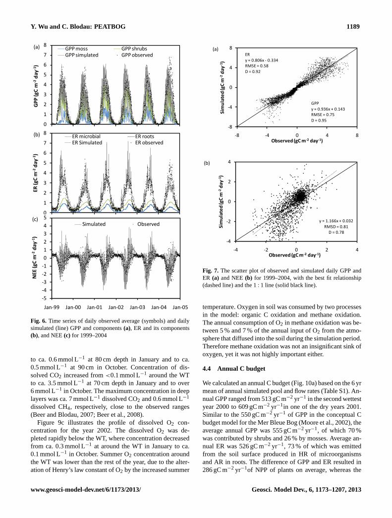
Y. Wu and C. Blodau: PEATBOG 1189
6
Figure 6. Time series of daily observed average (symbols) and daily simulated (line) GPP and
components (a), ER and its components (b), and NEE (c) for 1999 – 2004.
0
1
2
3
4
5
6
7
8
GP
P (g
Cm
-2d
ay-1
)
GPP moss GPP shrubsGPP simulated GPP observed
(a)
0
1
2
3
4
5
6
7
8
ER (g
Cm
-2d
ay-1
)
ER microbial ER rootsER Simulated ER observed
(b)
-5
-4
-3
-2
-1
0
1
2
3
4
5
Jan-99 Jan-00 Jan-01 Jan-02 Jan-03 Jan-04 Jan-05
NEE
(gC
m-2
day
-1)
Simulated Observed(c)
Fig. 6. Time series of daily observed average (symbols) and dailysimulated (line) GPP and components(a), ER and its components(b), and NEE(c) for 1999–2004
to ca. 0.6 mmol L−1 at 80 cm depth in January and to ca.0.5 mmol L−1 at 90 cm in October. Concentration of dis-solved CO2 increased from<0.1 mmol L−1 around the WTto ca. 3.5 mmol L−1 at 70 cm depth in January and to over6 mmol L−1 in October. The maximum concentration in deeplayers was ca. 7 mmol L−1 dissolved CO2 and 0.6 mmol L−1
dissolved CH4, respectively, close to the observed ranges(Beer and Blodau, 2007; Beer et al., 2008).
Figure 9c illustrates the profile of dissolved O2 con-centration for the year 2002. The dissolved O2 was de-pleted rapidly below the WT, where concentration decreasedfrom ca. 0.3 mmol L−1 at around the WT in January to ca.0.1 mmol L−1 in October. Summer O2 concentration aroundthe WT was lower than the rest of the year, due to the alter-ation of Henry’s law constant of O2 by the increased summer
7
Figure 7. The scatter plot of observed and simulated daily GPP and ER (a) and NEE (b) for 1999 -
2004, with the best fit relationship (dashed line) and the 1:1 line (solid black line).
-8
-4
0
4
8
-8 -4 0 4 8
Sim
ula
ted
(gC
m-2
day
-1)
Observed (gC m-2 day-1)
ER
y = 0.806x - 0.334RMSE = 0.58
D = 0.92
GPP
y = 0.936x + 0.143RMSE = 0.75
D = 0.95
(a)
y = 1.166x + 0.032
RMSD = 0.81D = 0.78
-4
-2
0
2
4
-4 -2 0 2 4
Sim
ula
ted
(gC
m-2
day
-1)
Observed (gC m-2 day-1)
(b)
Fig. 7. The scatter plot of observed and simulated daily GPP andER (a) and NEE(b) for 1999–2004, with the best fit relationship(dashed line) and the 1: 1 line (solid black line).
temperature. Oxygen in soil was consumed by two processesin the model: organic C oxidation and methane oxidation.The annual consumption of O2 in methane oxidation was be-tween 5 % and 7 % of the annual input of O2 from the atmo-sphere that diffused into the soil during the simulation period.Therefore methane oxidation was not an insignificant sink ofoxygen, yet it was not highly important either.
4.4 Annual C budget
We calculated an annual C budget (Fig. 10a) based on the 6 yrmean of annual simulated pool and flow rates (Table S1). An-nual GPP ranged from 513 gC m−2 yr−1 in the second wettestyear 2000 to 609 gC m−2 yr−1in one of the dry years 2001.Similar to the 550 gC m−2 yr−1 of GPP in the conceptual Cbudget model for the Mer Bleue Bog (Moore et al., 2002), theaverage annual GPP was 555 gC m−2 yr−1, of which 70 %was contributed by shrubs and 26 % by mosses. Average an-nual ER was 526 gC m−2 yr−1, 73 % of which was emittedfrom the soil surface produced in HR of microorganismsand AR in roots. The difference of GPP and ER resulted in286 gC m−2 yr−1of NPP of plants on average, whereas the
www.geosci-model-dev.net/6/1173/2013/ Geosci. Model Dev., 6, 1173–1207, 2013

1190 Y. Wu and C. Blodau: PEATBOG
8
Figure 8. Time series of (a) simulated daily CH4 flux (mg C m-2
day-1
) from 1999 to 2009, (b)
simulated growing season (day of year 120 to 330) daily CH4 flux (mg C m-2
day-1
) from 2004 to
2008 (blue area indicates the variation range as recoreded for the Mer Bleue Bog averaged from 12
collars (Moore et al. 2011, Fig. 2), (c) relationship between the simulated growing season daily and
(d) annual average CH4 flux (mg C m-2
day-1
) in log10 scale and the simulated daily water table
depth (m) from 1999 to 2009.
1
10
100
1000
Jan-99 Jan-01 Jan-03 Jan-05 Jan-07 Jan-09
CH
4fl
ux
(mgC
m-2
day
-1)
(a)
1
10
100
1000
120 150 180 210 240 270 300 330
20042005200620072008
(b)
y = 3.348x + 2.326
R² = 0.561
0
0.5
1
1.5
2
2.5
-1.0 -0.8 -0.6 -0.4 -0.2 0.0 0.2
log
of C
H4
flu
x (m
gCm
-2d
ay-1
)
Water table depth (m)
(c)
y = 1.110x + 1.671
R² = 0.427
1
1.1
1.2
1.3
1.4
-0.6 -0.5 -0.4 -0.3 -0.2
Water table depth (m)
(d)
Fig. 8. Time series of(a) simulated daily CH4 flux (mg C m−2 day−1) from 1999 to 2009,(b) simulated growing season (day of year 120to 330) daily CH4 flux (mg C m−2 day−1) from 2004 to 2008 (blue area indicates the variation range as recorded for the Mer Bleue Bogaveraged from 12 collars (Moore et al., 2011, Fig. 2),(c) relationship between the simulated growing season daily, and(d) annual averageCH4 flux (mg C m−2 day−1) in log10 scale and the simulated daily water table depth (m) from 1999 to 2009.
9
Figure 9. Simulated profiles of dissolved CO2 (a), dissolved CH4 (b), and dissolved O2 (c)
concentration (units: (umol·L-1
) in soil pore water in the year 2002. The black lines indicate water
table depth (m).
CO2 CH4 O2
(a) (b) (c)
Fig. 9.Simulated profiles of dissolved CO2 (a), dissolved CH4 (b), and dissolved O2 (c) concentration (units: (umol L−1) in soil pore waterin the year 2002. The black lines indicate water table depth (m).
average loss of C from the plants due to litter production andexudation was 296 C m−2 yr−1. The difference of 10 gC be-tween NPP and the sum of litter production and exudationcorresponded to the changes of biomass in the plants. Annualnet ecosystem production (NEP) was 29 gC m−2 yr−1, closeto the low end of the estimated 40.2 (±40.5) gC m−2 yr−1
(Roulet et al., 2007), which was based on 8 yr of observationsfrom 1999 onwards. The model simulated an annual CH4emission of 4 gC m−2 yr−1 of which 83 % stemmed fromgraminoid mediated emission. Emission of CH4 during thewet years of 2002 and 2004 were higher than in the dry years,as is the general trend observed in the Mer Bleue Bog andin other peatlands (Roulet et al., 2007). The simulated DOCexport was 15 gC m−2 yr−1, which was in agreement withthe estimated 14.9 (±3.1) gC m−2 yr−1 from 5 yr of runoffand 3 yr of DOC concentration measurements at the site.
The model suggested dissolved CO2 and CH4 loss in runoffwas 0.29 and 0.01 gC m−2 yr−1. These values were smallerthan the estimated and variable 1.77 gC m−2 yr−1(CO2) and0.05 gC m−2 yr−1(CH4) from the annual runoff in the MerBleue Bog drainage system (Billett and Moore, 2007). Fi-nally, the net ecosystem carbon balance (NECB= GPP-ER-CH4-DOC-DIC) was obtained as 10 (±60) gC m−2 yr−1.This value was smaller and more variable than field estimatesof 21.5 (±39) gC m−2 yr−1, although it fell within the possi-ble range of−105 to 50 gC m−2 yr−1 (Roulet et al., 2007).
4.5 Annual N budget
An annual N budget for the Mer Bleue Bog is il-lustrated based on the 6 yr average of simulated val-ues (Fig. 10b, Table S2). The wet annual N depositedfrom the atmosphere was 0.81 gN m−2 yr−1 onto the
Geosci. Model Dev., 6, 1173–1207, 2013 www.geosci-model-dev.net/6/1173/2013/

Y. Wu and C. Blodau: PEATBOG 1191
10
Figure 10. Carbon budget (a) and nitrogen budget (b) for the Mer Bleue peatland based on
simulated averages from 1999 to 2004. Pools are in g m-2
and fluxes are in g m-2
year-1
.
SOM C 963151
Decomposition 274
GPP 23
Mosses C 69
Graminoids shoot C 8
Shrubs shoot 116
GPP 146
GPP 386
Graminoids root C 18
Shrubs root 539
Litter 7
Litter 3 Litter 54 Exudates 52
Exudates 0
Litter 49
Litter 108
GEP 555
Shoot AR 143
DOC = 453
CO2 =530 CH4 = 39
CO2 production 252
CH4 production 11
CH4 emission 4
CO2 emission
384
Runoff DOC export 15
Runoff DIC export 0.31
AR 79
AR 6
AR 58
Plant C 751
AR 7
AR 120
(a)
Fig. 10.Carbon budget(a) and nitrogen budget(b) for the Mer Bleue peatland based on simulated averages from 1999 to 2004. Pools are ing m−2 and fluxes are in g m−2 yr−1.
peatland. About 95 % of the deposited N was absorbedby mosses right away. Nitrogen in the plants was associ-ated with the plant biomass and composition, which bothchanged little over the 6 yr. Annually, mosses exported0.82 gN m−2 yr−1 in litter and 0.02 gN m−2 yr−1 in exudatesto the soil N pools. For vascular plants these fluxes were2.97 gN m−2 yr−1 and 0.02 gN m−2 yr−1, respectively. N up-take was 1.68 gN m−2 yr−1, mostly by shrubs as NH+4 , andonly 0.3 % of N uptake occurred in form of DON. N2 fixa-tion was 0.96 gN m−2 yr−1. Considering N uptake, N litter-fall and N exudation, vegetation thus lost 0.38 gN m−2 yr−1,which represents 2.5 % per year over the simulation period.The NH+
4 pool was smaller than the annual production anduptake, implying a fast turnover of NH+4 in the soil. Otherdissolved N pools (NO−3 , N2O and NO) were 3 to 8 mag-nitudes smaller than the NH+4 pool in the model, and N2Oemission was negligible. Export of DON and DIN throughwater runoff was also very small and occurred at rates of0.04 gN m−2 yr−1 and 0.01 gN m−2 yr−1, respectively. Over-all, the OM pools received ca. 3.83 gN from plant litter pro-duction and exudation and lost 1.91 gN and 0.05 gN by min-eralization and runoff annually, which lead to an overall ac-cumulation of 1.43 gN m−2 yr−1 in the peat.
4.6 Sensitivity analysis
Sensitivity analysis is useful in quantifying the model re-sponses to changes in environmental drivers and other pa-rameters. We ran a series of simulations by adjusting key en-vironmental variables, such as precipitation, air temperatureand N deposition. Variations of these parameters were chosento be within the possible range of variability in temperate-boreal peatland ecosystems. We also adjusted parameters thatare most uncertain and potentially influence C and N cyclingin peatlands, such asQ10 values and the rate constants ofthe decomposition of SOM. The sensitivity of key C and Nfluxes, pools, and cycling rates, including GPP, AR, ER, HR,NEE, NECB, and C and N sequestration rates in the soil or-ganic matter, were examined. The sensitivity was tested byimposing changes in air temperature between−1 and+5with increments of 2◦C, and changes in precipitation be-tween−30 % and+30 % with increments of 15 %, whichwere in line with the scenario predictions of future climate(IPCC, 2007). The sensitivity to N deposition that coveredthe N deposition range in Europe was tested by imposing Ninput at 0.2, 1.4, 2, 2.5 and 3.2 gN m−2 yr−1. The sensitiv-ity to Q10 of labile (Q10,L) and recalcitrant (Q10,R) soil or-ganic matter were tested for−40 % and+40 % of the ambi-ent value, respectively. The potential decomposition constantk was tested with−25 % and+25 % of the ambientk for la-bile (kpotL) and recalcitrant (kpotL) in the sensitivity tests.
www.geosci-model-dev.net/6/1173/2013/ Geosci. Model Dev., 6, 1173–1207, 2013

1192 Y. Wu and C. Blodau: PEATBOG
The simulations were conducted for six years and averagedto compare with the baseline simulations (Table 5).
The sensitivity analysis showed that heterotrophic respi-ration was the most sensitive process in C cycling with re-gard to air temperature. Temperature increase had a nega-tive effect on the production of moss and a positive effecton the production of vascular plants, suggesting a favoringof vascular species in a warmer environment. The increasein AR in vascular plants with increasingT was greater thanthe increase in production of vascular plants, which led toa negative effect on NPP. In the model, theQ10 of respira-tion in plants was smaller than theQ10 of photosynthesis,suggesting that other controls constrain primary productionapart from temperature, such as N availability and soil mois-ture. The sensitivity of HR to temperature was greater thanthat of AR, resulting in preferential C loss from peat ratherthan from plant respiration with increasing temperature. Theimpact of temperature on ER was larger than on GPP andentailed a higher sensitivity of NEE to temperature as well.Although less CH4, DOC and DIC was exported when tem-perature was increased, NECB declined due to the greaterchange in NEE. Carbon sequestration was very sensitive totemperature in the model, and an increase of 1 degree in airtemperature would turn the modeled peatland from a C sinkinto a C source. Nitrogen sequestration was also negativelyaffected by temperature, but to a lesser extent.
The processes GPP, AR, HR were less sensitive to precip-itation than to temperature. This was not the case for the ex-port of dissolved C and CH4 fluxes. Decreasing precipitationpromoted primary production and autotrophic respiration invascular plants, while inhibiting the production of mosses.Increasing precipitation more strongly raised NPP in shrubsthan in mosses and had a negative effect on graminoids, sug-gesting vice versa that graminoids were more tolerant to dry-ness than shrubs and mosses. The increased NPP in shrubsresulted mostly from changing respiration rather than fromgross primary production. Respiration in the model has astronger dependency on soil moisture than GPP. In the analy-ses, HR was more sensitive to temperature and precipitationthan AR and NPP, and it was more sensitive to temperaturethan to precipitation (Table 5). A decrease in precipitation by30 %, corresponding to a decline of annual mean WT depthby 7 cm, led to an HR increase of 11 %. In contrast DICand DOC export declined by 36 % and 66 %, respectively.The decrease of dissolved C exports was owed to the di-minished runoff at lower WT position, despite more produc-tion of dissolved C with raised HR. As expected, CH4 fluxwas strongly positively related to precipitation. In contrast,elevated temperature decreased CH4 emission in the modelthrough the lowered WT depth (Table 5).
Interestingly, the sequestration rate of C was similarly sen-sitive to precipitation and to temperature, while the N seques-tration rate was much more sensitive to precipitation than totemperature. A decrease in precipitation by 30 % caused adecrease in C sequestration rate by 19 %, which is compara-
ble to the effect of an increase in temperature by 3 degrees.Meanwhile, the N sequestration rate decreased by 46 % withthe change in precipitation and by 10 % with the change intemperature. This outcome resulted from the different mech-anisms by which precipitation and temperature control thedecomposition of soil organic matter. In the model, loweringthe WT position via precipitation stimulated the decomposi-tion rate of labile and recalcitrant soil equally. On the otherhand, the temperature increases primarily the decompositionof recalcitrant OM due to a larger decompositionQ10 ofthis pool. As recalcitrant soil is present mostly in the deeperlayers and contains less N, the temperature effect on N se-questration was weakened. Therefore, if recalcitrant SOM ismore sensitive to temperature than labile SOM, as suggestedby many (Davidson and Janssens, 2006; Conant et al., 2008;Craine et al., 2010; Karhu et al., 2010), the function of peat-lands as N sinks will be more impaired than in predictionson models with equalQ10 values for labile and recalcitrantSOM.
Nitrogen deposition levels affect mostly plant related Cfluxes rather than soil derived fluxes. The sensitivity of GPPto N deposition was greater than to precipitation and tem-perature. Overall, the model suggests a strong promotionof graminoids over shrubs and mosses when the N deposi-tion increases. The effect of N on both GPP and NPP wasstronger in graminoids than in shrubs and mosses, due to thedifferent N use strategy of the PFTs in the model (Table 5).Graminoids have advantages because faster turnover rates al-low for instantaneous response to changes in N availability inthe plant-soil system. In comparison, shrubs and mosses cy-cle N in a more conservative manner and need lower levelsof N to keep photosynthesizing, hence these PFTs react moreslowly to increases in N availability. The NPP of graminoidsincreased non-linearly with the N deposition level, by 70 %with a 150 % increase and 560 % by a 300 % increase in an-nual N deposition (Table S3). This finding implies other con-straints on the NPP of graminoids at low N deposition levels.The main constraint was very likely N filtration by mosses,which was alleviated when mosses became N saturated athigher N deposition levels.
The NPP of shrubs was highest at moderate N depositionlevel of 2.6 gN m−2 yr−1, probably due to increased shadingeffects from the faster expansion of graminoids with more Ndeposition (Table S3). The NPP of mosses was negatively af-fected by N deposition, and only a slight promotion of GPPoccurred when N deposition was slightly raised. Very differ-ent from the effects of the climatic drivers, N deposition lev-els had hardly an effect on HR. Other C effluxes, includingdissolved C export, CH4 flux and AR were also less sensi-tive to N deposition than to temperature and precipitation.As GPP and ER were both positively affected by increasingN, the NEE, NECB and C sequestration rate of peat were notvery sensitive to N deposition. In contrast, N sequestrationin soil organic matter showed a strong positive relation to Ndeposition level.
Geosci. Model Dev., 6, 1173–1207, 2013 www.geosci-model-dev.net/6/1173/2013/
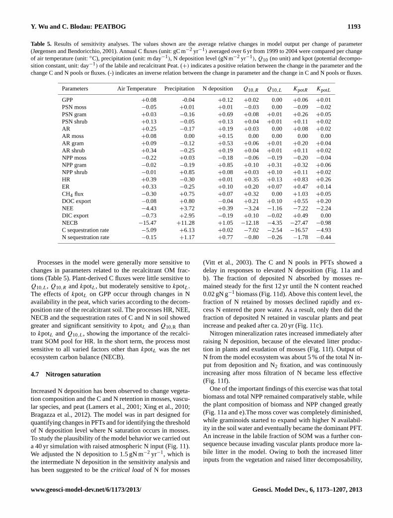
Y. Wu and C. Blodau: PEATBOG 1193
Table 5. Results of sensitivity analyses. The values shown are the average relative changes in model output per change of parameter(Jørgensen and Bendoricchio, 2001). Annual C fluxes (unit: gC m−2 yr−1) averaged over 6 yr from 1999 to 2004 were compared per changeof air temperature (unit:◦C), precipitation (unit: m day−1), N deposition level (gN m−2 yr−1), Q10 (no unit) and kpot (potential decompo-sition constant, unit: day−1) of the labile and recalcitrant Peat. (+) indicates a positive relation between the change in the parameter and thechange C and N pools or fluxes. (-) indicates an inverse relation between the change in parameter and the change in C and N pools or fluxes.
Parameters Air Temperature Precipitation N depositionQ10,R Q10,L KpotR KpotL
GPP +0.08 -0.04 +0.12 +0.02 0.00 +0.06 +0.01PSN moss −0.05 +0.01 +0.01 −0.03 0.00 −0.09 −0.02PSN gram +0.03 −0.16 +0.69 +0.08 +0.01 +0.26 +0.05PSN shrub +0.13 −0.05 +0.13 +0.04 +0.01 +0.11 +0.02AR +0.25 −0.17 +0.19 +0.03 0.00 +0.08 +0.02AR moss +0.08 0.00 +0.15 0.00 0.00 0.00 0.00AR gram +0.09 −0.12 +0.53 +0.06 +0.01 +0.20 +0.04AR shrub +0.34 −0.25 +0.19 +0.04 +0.01 +0.11 +0.02NPP moss −0.22 +0.03 −0.18 −0.06 −0.19 −0.20 −0.04NPP gram −0.02 −0.19 +0.85 +0.10 +0.31 +0.32 +0.06NPP shrub −0.01 +0.85 +0.08 +0.03 +0.10 +0.11 +0.02HR +0.39 −0.30 +0.01 +0.35 +0.13 +0.83 +0.26ER +0.33 −0.25 +0.10 +0.20 +0.07 +0.47 +0.14CH4 flux −0.30 +0.75 +0.07 +0.32 0.00 +1.03 +0.05DOC export −0.08 +0.80 −0.04 +0.21 +0.10 +0.55 +0.20NEE −4.43 +3.72 +0.39 −3.24 −1.16 −7.22 −2.24DIC export −0.73 +2.95 −0.19 +0.10 −0.02 +0.49 0.00NECB −15.47 +11.28 +1.05 −12.18 −4.35 −27.47 −0.98C sequestration rate −5.09 +6.13 +0.02 −7.02 −2.54 −16.57 −4.93N sequestration rate −0.15 +1.17 +0.77 −0.80 −0.26 −1.78 −0.44
Processes in the model were generally more sensitive tochanges in parameters related to the recalcitrant OM frac-tions (Table 5). Plant-derived C fluxes were little sensitive toQ10,L, Q10,R andkpotL, but moderately sensitive tokpotL.The effects ofkpotL on GPP occur through changes in Navailability in the peat, which varies according to the decom-position rate of the recalcitrant soil. The processes HR, NEE,NECB and the sequestration rates of C and N in soil showedgreater and significant sensitivity tokpotL andQ10,R thanto kpotL andQ10,L, showing the importance of the recalci-trant SOM pool for HR. In the short term, the process mostsensitive to all varied factors other thankpotL was the netecosystem carbon balance (NECB).
4.7 Nitrogen saturation
Increased N deposition has been observed to change vegeta-tion composition and the C and N retention in mosses, vascu-lar species, and peat (Lamers et al., 2001; Xing et al., 2010;Bragazza et al., 2012). The model was in part designed forquantifying changes in PFTs and for identifying the thresholdof N deposition level where N saturation occurs in mosses.To study the plausibility of the model behavior we carried outa 40 yr simulation with raised atmospheric N input (Fig. 11).We adjusted the N deposition to 1.5 gN m−2 yr−1, which isthe intermediate N deposition in the sensitivity analysis andhas been suggested to be thecritical load of N for mosses
(Vitt et al., 2003). The C and N pools in PFTs showed adelay in responses to elevated N deposition (Fig. 11a andb). The fraction of deposited N absorbed by mosses re-mained steady for the first 12 yr until the N content reached0.02 gN g−1 biomass (Fig. 11d). Above this content level, thefraction of N retained by mosses declined rapidly and ex-cess N entered the pore water. As a result, only then did thefraction of deposited N retained in vascular plants and peatincrease and peaked after ca. 20 yr (Fig. 11c).
Nitrogen mineralization rates increased immediately afterraising N deposition, because of the elevated litter produc-tion in plants and exudation of mosses (Fig. 11f). Output ofN from the model ecosystem was about 5 % of the total N in-put from deposition and N2 fixation, and was continuouslyincreasing after moss filtration of N became less effective(Fig. 11f).
One of the important findings of this exercise was that totalbiomass and total NPP remained comparatively stable, whilethe plant composition of biomass and NPP changed greatly(Fig. 11a and e).The moss cover was completely diminished,while graminoids started to expand with higher N availabil-ity in the soil water and eventually became the dominant PFT.An increase in the labile fraction of SOM was a further con-sequence because invading vascular plants produce more la-bile litter in the model. Owing to both the increased litterinputs from the vegetation and raised litter decomposability,
www.geosci-model-dev.net/6/1173/2013/ Geosci. Model Dev., 6, 1173–1207, 2013

1194 Y. Wu and C. Blodau: PEATBOG
12
Figure 11. Simulated C pools (a), N pools (b) and NPP (e) in plants and PFTs, N uptake rate by in
plants and sequestration rate in peat (c), N absorbed by moss and N content in mosses (d), N
mineralization rate and N output from peat (f) at annual wet N deposition of 1.5g N m-2
yr-1
from
1999 to 2039.
0
200
400
600
800
1000
1200
1990 2000 2010 2020 2030 2040
Pla
nts
C (
gC m
-2)
total moss shrub gram
(a)
0
10
20
30
40
50
60
1990 2000 2010 2020 2030 2040
Pla
nts
N (g
N m
-2)
total moss shrub gram
(b)
0
100
200
300
400
500
1990 2000 2010 2020 2030 2040
NP
P (g
C m
-2)
total moss shrub gram
(e)
0
1
2
3
4
5
6
7
1990 2000 2010 2020 2030 2040
N u
pta
ke ra
te (g
N y
r-1)
soil moss shrub gram
(c)
0.00
0.05
0.10
0.15
0.20
0.25
0
1
2
3
4
5
6
1990 2000 2010 2020 2030 2040
N o
utp
ut (
gN m
-2yr
-1)
N m
ine
rali
zati
on
rate
s (g
N m
-2yr
-1)
N mineralization rate N output
(f)
0.00
0.05
0.10
0.15
0.0
0.4
0.8
1.2
1.6
1990 2000 2010 2020 2030 2040
N c
on
ten
t (gN
gC
-1)
N a
bso
rbe
d (g
N y
r-1)
N absorbed by moss N content in moss
(d)
Fig. 11. Simulated C pools(a), N pools (b) and NPP(e) in plants and PFTs, N uptake rate by in plants and sequestration rate in peat(c), N absorbed by moss and N content in mosses(d), N mineralization rate and N output from peat(f) at annual wet N deposition of1.5 g N m−2 yr−1 from 1999 to 2039.
the sequestration rate of C in soil first accelerated but thenslowed after the NPP had peaked (Fig. 11e).
5 Discussion
5.1 Carbon fluxes and environmental controls
The fluxes GPP, ER and NEE are the essential componentsin C cycling that express the ability of peatland ecosystemsin assimilating and dissimilating C and exchange the ele-ment with the atmosphere. Overall, the model simulationsshowed good agreement in daily C fluxes, belowground Cconcentration and annual C and N budgets with empiricaldata. However, a bias occurred towards underestimating sim-ulated GPP (i.e. slope= 0.936), underestimating simulatedER (i.e. slope= 0.806) and overestimating simulated NEE(i.e. slope= 1.166). These biases are within the bias rangeof the other models that primarily focus on C cycling (e.g.MWM, PCARS). The model performance differed in thatin MWM and PCARS the simulated ER was overestimated,while it was underestimated in the PEATBOG model.
The 6 yr averaged annual GPP demonstrates the abilityof the model in simulating overall productivity, as only asmall deviation of 5 gC m−2 was recorded against an empir-ically determined large average GPP of 550 gC m−2 at thesite (Moore et al., 2002). Also the trends in interannual vari-ation of GPP with precipitation and temperature were largelymet. Noteworthy is for example the decline in GPP in theextremely dry year 1999, when dryness had a large impacton the GPP of mosses, and the high GPP in the warm andwet year of 2001 (Figs. 5b and 6a). While overall modelperformance was good some deviation from empirical mea-surements were illustrated by the analysis as well. AnnualGPP was overestimated by 32 to 85 gC m−2 yr−1 from year2000 to 2003 and underestimated by 70 to 123 gC m−2 yr−1
for the remaining years by the model simulations (Table 6).The discrepancy of annual GPP simulations ranged from 7 %to 18 % and was not significant (P = 0.737,n = 2192). Thesimulated GPP fraction of shrubs was 70 %, ranging from66 % in the simulated wettest year of 2004 and 78 % in thedriest year 1999. This range was similar to the model out-put of MWM that ranged from 61 % to 67 % (St-Hilaire etal., 2010) and smaller than the shrub related fraction of GPP
Geosci. Model Dev., 6, 1173–1207, 2013 www.geosci-model-dev.net/6/1173/2013/

Y. Wu and C. Blodau: PEATBOG 1195
of 80 % to 85 % reported from the PCARS model (Frolk-ing et al., 2002). Inter-annual variation of GPP for PFTs wascorroborated by observation (Bubier et al., 2003): GPP ofmosses increased from dry to wet years from 4 % to 48 %,whereas GPP of shrubs was at its lowest levels in the wetyears. In comparison to other models (St-Hilaire et al., 2010;Dimitrov et al., 2011), the inhibition of GPP of shrubs due todryness is less effective in our model.
On the daily timescale some weakness of the model in re-sponding to weather conditions became visible. In general,the simulated GPP was deficient in capturing short-term ex-treme fluxes. All large underestimates (>2 gC m−2 day−1) inthe GPP simulation occurred during mid-summer in the twowet years 2000 and 2005, when GPP in the peatland waslarger than 5 gC m−2 day−1, except for two days in late sum-mer. The likely reason for the lack of adequate model per-formance during this time are the maximum photosynthesisrates that are set for each PFT and the impossibility to coverthe daily observed extreme values that were averaged fromhalf hour records in the measurements. This disadvantagealso occurred in other models with maximum rate settingsthat are based on the Farquhar photosynthesis model (e.g.MWM). We also noticed that most of the underestimates thatoccurred in 2004 were associated with frequent heavy pre-cipitation that raised production instantly. In the model, theproduction of mosses is the only PFT that reacts to precip-itation directly through the water content in thecapitulumof mosses. The indirect controls of precipitation on the pro-duction of vascular plants via WT depth is likely the rea-son of the underestimated promotion of photosynthesis byfrequent precipitation, especially when other controlling fac-tors (i.e. temperature, light) are within the optimal range.For example, a peak of measured daily GPP was observedduring late July 2004, during one of the periods that under-estimated GPP. At this time precipitation was continuous at>10 mm day−1and temperature was within an optimal range(20± 3◦C).
The overestimation of GPP mainly occurred during lateMay to early June in the dry years (2001 to 2003) whenPAR was comparably strong (>600 umol m−2 s−1). Duringthose days, the model predicted GPP of mosses and shrubs toreach a level above 1.2 gC m−2 day−1 and 2 gC m−2 day−1,respectively. Daily measured GPP in the Mer Bleue Bogwas found to be significantly albeit weakly related to PAR(P < 0.001;r2
= 0.19) (Moore et al., 2006). In the model,this relationship is significantly stronger (r2
= 0.75), due toneglecting the non-linearity of leaf response to light in theintegration of canopy photosynthesis using just Beer’s law.The non-linearity of leaf response to light is related to the di-urnal effects on the canopy. It includes for example optimizednitrogen distribution in plant canopies, different responsesto light in sun and shade leaves, and variation of stomatalconductance with light levels (Thornley, 2002; Hikosaka,2003). Late May to early June was also the period whennew biomass is built up, which affects the distribution of
N within the plants. For example, both total N content andchlorophyll-a concentration in evergreen shrub foliage werelow in spring and increased steadily to early June, as shownin measurements (Moore et al., 2006). The model lacks sep-arated N pools in foliage and stems, where N content couldshow great variations due to phenology, which might be thereason of the overestimation of GPP in late spring.
The fluxes ER and NEE represent the gross and net releaseof CO2 from peatlands, and largely determine the C balanceof the ecosystem. The model reproduced the composition ofER, where HR contributed half of the total ER, while theother half was almost equally shared by AR in shoots and ARin roots, as approximately suggested by field measurements(Moore et al., 2002). However, the standard deviation of thesimulated annual ER and NEE was larger than that in fieldestimates (50 % and 40 %), suggesting a larger inter-annualvariation than measured in the field. The modeled annual ERranged from 430 gC m−2 yr−1 to 573 gC m−2 yr−1, with anaverage of 526 gC m−2 yr−1 (Table S1), which is close to theflux quantified as 461 gC m−2 yr−1 (Lafleur et al., 2001). Theannual discrepancy ranged from 3 % to 17 %, with an excep-tion of 25 % in 2004, when the highest summer WT occurred(Table 6). The underestimation of ER was probably causedby the simulated WT depth (Fig. 5b) that was 5 to 10 cmhigher than measured in summer when both autotrophicrespiration (AR) and heterotrophic respiration (HR) werepotentially high. The modeled NEE showed similar inter-annual patterns to ER with the annual error being between35 gC m−2 yr−1 to 18 gC m−2 yr−1. The largest deviation ofsimulated NEE from measurements was 106 gC m−2 yr−1 in1999, when GPP was under- and ER overestimated.
The ER was also overestimated from 1999 and 2003(Fig. 6b). To identify the reasons, we calculated the devia-tion between measured and model daily ER, and regressedit against the deviation of measured and modeled daily tem-perature. According to this approach the overestimate of ERfrom 1999 to 2003 could be explained by an overestimateof soil temperature (r2
= 0.26), especially during summer(r2
= 0.68). Both ER and HR were strongly correlated tosoil temperature at 0.2 cm depth withr2 of 0.88 and 0.83,respectively (n = 2193). The strong temperature dependenceof ER and HR was associated with theQ10 values used inthe model for the temperature effects on HR rates. Differentfrom other models, whereQ10 values were set to 2 for mi-crobial respiration in soil,Q10 value for the decompositionof recalcitrant OM (3.3) was set to be larger than for labileOM (2.3). TheseQ10 values were in line with some of themost recent results (Davidson and Janssens, 2006; Conantet al., 2008, 2010; Karhu et al., 2010), their application im-plies a stronger increase in C loss from peatlands in a warmerclimate. It has to be noted that some have assumed the valueof Q10 for labile OM to be larger (Liski et al., 1999; Giardinaand Ryan, 2000; Thornley and Cannell, 2001) than or simi-lar to (Fang et al., 2005) that of recalcitrant OM; in this caseclimate change effect on NEE may not be as extraordinary as
www.geosci-model-dev.net/6/1173/2013/ Geosci. Model Dev., 6, 1173–1207, 2013

1196 Y. Wu and C. Blodau: PEATBOG
Table 6. Observed (Obs.), simulated (Sim.), and the difference (D) between observed and simulated annual GPP, ER and NEE (units:gC m−2 yr−1) and summer average water table depth (unit: m) from 1 May to 30 October for 6 yr for the Mer Bleue Peatland.
GPP ER NEE WTD
Year Obs. Sim. D Obs. Sim. D Obs. Sim. D Obs. Sim. D1999 593 523 −70 537 573 36 −56 42 99 −0.49 −0.61 −0.122000 481 513 32 456 470 14 −25 −47 −22 −0.34 −0.33 0.012001 524 609 85 532 581 49 8 −33 −41 −0.48 −0.52 −0.042002 495 560 65 487 570 83 −9 4 13 −0.51 −0.50 0.012003 513 562 49 498 533 35 −15 −32 −17 −0.46 −0.49 −0.032004 686 563 −123 574 431 −143 −112 −134 −22 −0.40 −0.37 0.03
has been anticipated otherwise. The sensitivity analysis onQ10 and potential decomposition rates for our model high-lighted the importance of the recalcitrant OM over the labileOM for the C cycling in peatlands (Table 5).
The Q10 values derived from the first order exponentialequations of the simulated ER and HR were only 2.56 and1.97, respectively. TheQ10 for HR was thus smaller thaneither of theQ10 for labile or recalcitrant OM, revealing theimportance of other factors that confound the temperature re-sponse of HR. The WT depth was the most important factoraffecting the calculatedQ10 values withr2 of 0.75 betweenthe average summer WT depth and the calculatedQ10 values.In summer, the low soil moisture in the most upper peat lay-ers counteracted the potential enhancement of respiration bytemperature. Nevertheless, the sensitivity analysis suggesteda lesser effect of WT depth than of soil temperature on CO2fluxes (Table 5). The daily simulated WT depth moderatelycorrelated with ER (r2
= 0.51,n = 2192), with r2 rangingfrom 0.19 in the wet year 2000 to 0.79 in the dry years. Al-though stronger than reported from empirical studies, this re-lationship was in a broad agreement with field results as faras the trend of tighter correlation in dry years goes (Bubier,2003; Lafleur et al., 2005b; Blodau et al., 2007).
The CH4 fluxes modeled with our novel thermodynamic-kinetic approach were in a reasonable range but smaller andtheir seasonal pattern less pronounced than obtained withchamber measurements at the Mer Bleue Bog (Moore et al.,2011). We attribute this difference to the variability of in situplant cover and a higher mean water table position of the12 gas flux collars of the field study. The collars were notonly located in hummocks and lawns but also in hollows.The observed average WT depth was−35 (±8.4 cm) for the12 collars from 2004 to 2008, whereas the simulated aver-age WT depth was−41 cm for the same time period. Dueto the generally observed exponential increase in emissionswith raising water table (Moore et al., 1998), even a smallnumber of sampled wet locations may lead to much largeremissions than simulated in the model, which represents ahummock situation. The large discrepancy after summer wasvery likely due to the effects of vegetation transport on CH4flux, which was the most important control on the CH4 flux
from September to November over 5 yr (Moore et al., 2011).In the model, graminoid cover was less than 1 % during thesimulation period, whereas the graminoid cover ranged from0 to 100 % in the 12 collars. Comparing model output to oneof the gas flux collars similar in water table and graminoidcover (collar 8, Table 2, Moore et al., 2011) with daily CH4flux between 10 to 100 mg m−2 day−1, a closer model fit wasobtained. In this collar, as in our model, CH4 emission in-creased less in summer than in the more grass-rich collars(Moore et al., 2011).
The growing season log10 values of both daily and annualCH4 fluxes showed moderately strong relations with WTdepth (r2
= 0.56,n = 2119 andr2= 0.45,n = 11) (Fig. 8c
and d). The outliners were the degassing events, which oc-curred when water table was crossing the boundaries of peatlayers in the model. The WT depth during the growing seasonshowed differing effects on CH4 fluxes in dry years and wetyears, as was also found in the field (Moore et al., 2011). Ac-cording to the model results, the lowest dependence of CH4flux on the WT depth occurred in the dry years and the high-est dependence in the wetter years. This finding is in con-flict with relations obtained from field data, where CH4 emis-sions were less related to summer WT depth in wetter years.The annual variation in CH4 production is less pronouncedthan in CH4 fluxes (Table S1); this implies that changes inthe transport mode of CH4 might offset the well-known WTcontrol on methanogenesis. For example, the root biomassof graminoids, that provide conduits for CH4 transport, wasnegatively correlated with WT depth and CH4 fluxes. In thedry years, graminoid root biomass increased with decliningWT in the model, due to more reallocation of newly pro-duced biomass to roots for accessing soil water. This adap-tation also increased the transport of CH4 from the deeperpeat. Overall, the model was able to simulate the variation ofCH4 fluxes with the change of environmental controls, andrevealed some interesting dynamic interactions with ecosys-tem structure that warrant further analysis in the future.
Geosci. Model Dev., 6, 1173–1207, 2013 www.geosci-model-dev.net/6/1173/2013/

Y. Wu and C. Blodau: PEATBOG 1197
5.2 N budget and N saturation
The simulated N budget identified the Mer Bleue Bog asa currently N-limited ecosystem and sink for the element.The immobilization of deposited N by mosses was at a max-imum level of 95 %, including both the retention of N inthe capitulum of Sphagnummosses and indirect retentionvia their stems. In the simulation of N saturation, the modelwas able to track the effect of N deposition in differentcompartments of the ecosystem. The N content in mossespeaked at 0.02 gN g−1 biomass, similar to the field obser-vations of 0.015 to 0.024 gN g−1 biomass (Heijmans et al.,2001; Granath et al., 2009; Xing et al., 2010). The simu-lated increase in soil organic matter mineralization was inagreement with most fertilization experiments (Bragazza etal., 2006; Breeuwer et al., 2008). It was closely related to achange in peat chemistry, such as reflected in the size of thelabile OM fraction in peat and its C/N ratio, as observed ina 7-year fertilization experiment (Bragazza et al., 2012). Themodel also successfully simulated the maintenance of totalPFT biomass and production with dramatic changes in thePFT composition, as observed in many N fertilization exper-iments (Bubier et al., 2007; Juutinen et al., 2010).
Uptake of DON, which has not been considered in peat-land models previously, represented a negligible fraction (ca.0.2 %) of the total N uptake by the roots of vascular plants.However, the turnover rate of DON was extremely high, re-vealing the strong demand and potential uptake of DON bythe roots of vascular plants. The fast turnover rate (Kiellandet al., 2007) and the large potential uptake of DON (Kah-men et al., 2009) were previously reported from field exper-iments on boreal forest and three intermediate N availablesystems, respectively. The model showed that the primarylimitation on the uptake of DON was the DON concentrationin the soil water, which was also suggested for boreal for-est (Kielland et al., 2006) and forAnthoxanthum odoratumin a fertilized experimental site (Sauheitl et al., 2009). Con-sequently, DON uptake will be more important when thereis more bio-available DON in the soil. Although not shownhere, the DON uptake accounted for 16 % of the total N up-take of shrubs after 40 yr of N deposition of 1.5 gN m−2 yr−1
in the N saturation simulation.The nitrogen saturation simulation further showed that the
impact of N deposition developed only after a considerabletime lag (Fig. 11). Except for mineralization and N output,the C and N pools and fluxes remained stable in the first 12simulation years until N became saturated in mosses. Onlyafter that point, the N retention in vascular plants and peatincreased dramatically and changed the peatland into grassdominated within 8 yr. A delay of 12 yr in the occurrence ofeffects of N fertilization reveals the importance of accumu-lated N deposition rather than annual N deposition.
6 Conclusions
The PEATBOG model has been developed for the purpose ofanalyzing coupled C and N cycling on a process-level and adaily to multi-year timescale. Our objective was to concep-tually consistently integrate vegetation, soil biogeochemistryand soil water dynamics. The model was further designed tobe sensitive to changes in N deposition, temperature and pre-cipitation. PEATBOG thus integrates a vegetation submodelcomprising three PFTs with a soil and water biogeochemi-cal model providing high spatial and process resolution. Itconsistently emphasizes mass balance principles and the dy-namic interplay of production, consumption and transloca-tion of materials throughout the ecosystem. PEATBOG isable to generate soil physical conditions and plant compo-sition internally and thus requires only a few site specific pa-rameters on geological location, local climate and initial veg-etation composition for simulations. The PEATBOG modelwas effective in reproducing current C and N cycles in anorthern peatland with some weaknesses in displaying cor-rect short-term dynamics of C cycling during extreme me-teorological periods. It was adequately sensitive to broaderchanges in climate and N deposition and reproduced a con-siderable range of empirical findings related to effects of in-ter annual meteorological variability and N deposition (e.g.the temperature control on soil respiration, change in PFTcomposition while total C pool and NPP in plants remainedrobust).
In this paper we presented the components and structureof the model and evaluated the general model performanceand sensitivity. The sensitivity analyses and the simulationof increased N deposition demonstrated the model’s utility inanalyzing the effects of climate change and N deposition onthe C and N cycles of peatlands. The analyses further illus-trated its usefulness in hypothesis-building that could assistin designing empirical studies examining ecosystem changesover the long term.
In terms of application, the model is suitable for investi-gating the mechanisms of observed changes in peatland Cand N fluxes due to changes in meteorological drivers and Ninput. Alternatively, the model could be a tool for assessinglong-term scenarios of global change. The multi-layer struc-ture of the soil submodel also allows for the integration ofother belowground processes in the future, such as SO2−
4 re-duction, to explicitly model CH4 production on account ofthe competition among electron acceptors. Although the CH4production was modeled conceptually from an electron com-petition perspective, which we did not detail in this paper, italso produced reasonable annual fluxes and depth profiles ofCH4 concentration, which hold promise for future analysesof CH4 dynamics.
www.geosci-model-dev.net/6/1173/2013/ Geosci. Model Dev., 6, 1173–1207, 2013

1198 Y. Wu and C. Blodau: PEATBOG
Appendix A
Equations
A1 Environment submodel
di = distance between the adjacent layers (m),i = layernumber,f = factors, frac= fraction, PAI= plant leaf area in-dex (m2), Vi = volume of layeri (m3), VWC= volumetricwater content (m3 m−3), zi = depth of layeri (m).
WS(t) = Pre+ Snow− EPT− Runoff (A1)
EPT= fWT,EPT · fPAI,EPT · fT ,EPT · PAR· r EPT0 (A2)
fPAI EPT = 1− e−PAI (A3)
Runoff={Transmissivity· local slope· (WT − 0.75) if Pre+ Snow+ WS< WSmax
Pre+ Snow else(A4)
Advection= Advection frac· Runoff (A5)
runoffL,i = (Runoff− Advection) · Khi/∑
i
Khi (A6)
Khi = 10f saturatedKhi+f VWC Khi (A7)
WT =
2 · WS− 0.8 if WS < 0.2WS− 0.6 if 0.2 < WS< 0.6
0 if WS ≥ 0.6(A8)
VWCi = VWCmin,i + (porosityi − VWCmin,i)/(1+ α |suction|n
)(1−1/n) (A9)
Suctioni =
{(zi − WT) + Suctionsaturatedi if zi > WT
Suctionsaturated else(A10)
Porosityi = (1− 0.0107· (−zi · 100)0.507)/1.5 (A11)
O2,i(t) = O2diff top,i − O2diffbot,i − CO2proi
− 2 · CH4oxi O2,i (A12)
T (z, t) = µT + σT fsnow (A13)
exp
√πz2
i
�Kthermal,i
sin
2π(t − tl)
�+
√πz2
i
�Kthermal,i
DL = 360· arccos(− tan(Latitude· π/180)
· tan(declination· π/180))/15π (A14)
declination= 23.45· sin(2π · (284+ doy)/365) (A15)
WCcap(t) = rain inceptedmoss− EPTmoss (A16)
rain inceptedmoss= min((WCcap,max− WCcapitulum),
Pre· LAI moss· drain/Bsh,moss) (A17)
EPTmoss=
{WCcap· EPT rmoss if Pre= 0
0 else(A18)
WCmoss= WCcap+ capillary rise (A19)
capillary rise= (A20)
max(WCcapmin,min(WCcapmax,22· exp6.5·WT))
BDi = 0.0107· (−100· di)0.567 (A21)
PeatCi = BDi · Vi · 1003 (A22)
DMinitial i = DMconc initiali · VWCi · Vi (A23)
Nabsorbedmoss= Nload· r Nabsorb/365 (A24)
A2 Vegetation
B = biomass, conc= concentration, DIC= CO2CH4,DIN = NO−
3 , NH+
4 , j = plant functional typej (1 = mosses,2 = graminoids, 3= shrubs), li= litter, M = carbon ornitrogen, Na= area based nitrogen content (gN m−2),Q = substrate or structural, reallo= reallocation of carbonor nitrogen, rec= recycle, Rm = maintenance respiration,Rg= growth respiration, upt= uptake,X = sh, rt, stem, leaf,fineroot, coarse root.
BX,j = XstrucCj/Cconcj (A25)
MconcX,Q,j = MX,Q,j/BX,j (A26)
rt distribi,j =
rt k−100·zi−1j − rt k
−100·zi
j if i < irooting,j
rt k−100·zi
j − rt k−100·z20j if i = irooting,j
0 else
(A27)
Brt,i,j = Brt,j · rt distribi,j (A28)
f Brt,i,j = Brt,j · rt distribi,j/∑j
Brt,j (A29)
li Mrt,q,i = Li fracq ·
∑j
(li Mrt,j · rt distribi,j ) (A30)
finertSi,j = 0.01· finertBi,j · PI · LV j/densityfinertj (A31)
LV j = 1/πr2cylinder,j (A32)
MX,Q,j (t) = growthMX,j − li MX,j (A33)
li Csh,struc,j = Csh,struc,j · rmort,sh,j
· fT ,sh,j + rdeciduous· Cleaf,struc,j (A34)
li Crt,struc,j = Crt,struc,j · rmort,rt,j · fT ,rt,j (A35)
li NX,struc,j = li CX,struc,j/CNratioX,struc,j (A36)
Csh,subs,j (t) = CanopyPSNCj + li rec Csh,j
− growthCsh,j − li Csh,subs,j − Rmsh,j
− Rgsh,j − realloCj − exuCsh,j (A37)
CanopyPSNCj = leafPSNj · DayLength
·
(1− e−kext,j LAI j
)/kext,j (A38)
LAI j = SLAj · Cleaf,struc,j (A39)
leafPSNj ={αjkext,iLI i + Pmax,j =√[(αjkext,j LI jPmax,j )2 − 4ξαjkext,j LI jPmax,j ]
}(A40)
LI j = (A41)
Geosci. Model Dev., 6, 1173–1207, 2013 www.geosci-model-dev.net/6/1173/2013/

Y. Wu and C. Blodau: PEATBOG 1199{PAR· kext,shrub· e
−kext,shrub·LAI shrub · kext,gram· e−kext,gram·LAI gram if j = 1PAR if j = 2
PAR· kext,gram· e−kext,gram·LAI gram if j = 3
αj = α0fCO2,α,jfT ,α,jfm,α,j (A42)
fT ,α,j =
{0 if Snow> 0.2
min(1− 0.001125· (Tair − 14),1) else(A43)
fCO2,α = 1− 0.3× 10⁻⁶/0.0015· CO2,air (A44)
fm,α,j = fM,Pmax,j =
{a2m,sh,j if j > 1
fmoss,PSN else(A45)
Pmax,j = Pmax,20,jfCO2,Pmax,jfT ,Pmax,jfM,Pmax,j
fgs,Pmaxfseason,PmaxfN,P max,j (A46)
fN,Pmax,j = (A47){max(0,min(1,aPNUE,j · Naj + bPNUE,j )) if j > 1max(0,min(1,aPNUE,j · Naj + bPNUE,j )) if j = 1∩ Namoss< Namax,moss
fN,toxic else
Naj = Nsh,subs,j/SLAj (A48)
RmX,j = rRmX,j · CX,struc,j · fm,X,j · fT ,X,r,j (A49)
fT ,X,r,j = Q(Tair−25)/1010,X,r,j (A50)
growthCX,j = CX,struc,j · r growthX,j · f TX,j · fmX,j ·
k growthX,j · (A51)
CconcX,subs,j
kmgrowthCj + CconcX,subs,j·
NconcX,subs,j
kmgrowthNj + NconcX,subs,j
fm,X,j =
{a20m,X,j if j = 2
a10m,X,j if j = 3
(A52)
fT ,j =
{T
qj (45− Tj )/Tref(45− 20) if 0 < Tj < 45
0 else(A53)
RgX,j = growthCX,j · (1− k growthX,j )/k growthX,j (A54)
li MX,subs,j = li BX,j · MconcX,subs,j · li M fracX,subs,j (A55)
li C fracX,subs,j =(li C fracX,subs,j,minkli ,subsC+ CconcX,subs,j
)/(
kli ,subsC+ CconcX,subs,j)
(A56)
li rec CX,subs,j = li recNX,subs,j · CNratiorec (A57)
realloMj =∣∣Mconcsh,subs,j − Mconcrt,subs,j
∣∣/(ρM,j/Bsh,j + ρM,j/Brt,j
)(A58)
Crt,subs,j (t) = realloCj + li rec Crt,subs,j
+ Cuptj − li Crt,subs,j − growthCrt,j − Rmrt,j
− Rgrt,j − exuCrt,j (A59)
exuCX,j = r exuX,j · fmX,j · f TX,j · CX,subs,j (A60)
Cuptj = Nuptj · CNratiouptake (A61)
Nsh,subs,j (t) = (A62){Nabsorbedmoss+ li rec Nsh,subs,j + N2fixmoss− growthNsh,j − li Nsh,subs,j − exuNX,j if j = 1
realloNj + li rec Nsh,subs,j − growthNsh,j − li Nsh,subs,j else
li rec NX,subs,j = li NX,subs,j · li rec NfracX,subs,j (A63)
li rec NfracX,subs,j = li rec NfracX,subs,j,maxkrec subsN
/(NconcX,subs,j + krec subsN
)(A64)
li NX,subs,j = frac li NX,subs,j · NX,subs,j · li BX,j (A65)
frac li NX,subs,j = frac li NX,subs,j,min · kli subsN/(kli subsN+ NconcX,subs,j
)(A66)
growthNX,j=growthCX,j· NconcX,j/Cconcj (A67)
N2fixmoss= fracN2fixmoss· TotalN2fix (A68)
exuNX,j = exuCX,j/CNratioX,subs,j (A69)
Nrt,subs,j (t) = li rec Nrt,subs,j + Nuptj− realloNj − growthNrt,j
− li Nrt,subs,j − exuNrt,j (A70)
Nuptj = (A71){0 if j = 1
(∑i
DONupti,j +∑i
NH+
4 upti,j+∑i
NO−
3 upti,j ) · 14/1000 else
DINupti,j = DINupt poti,j · f TDINupt,i/f CNsubs,j (A72)
DINupt poti,j = (A73){0 if i > irooting,j
Vm,DIN · DINconci · finertSi,j/(km,DIN + DINconci
)else
f TNH+
4 upt,i,j =
{0 if Tsoil,i < −5
0.2Tsoil,i + 1 if −5 < Tsoil,i < 01 if Tsoil,i > 0
(A74)
f TNO−
3 upt,i,j = Q(T soil,i−10)/1010,NO−
3 upt(A75)
f CNsubs,j = 1+ km,C,Nupt · (1+ Nconcrt,subs,j/km,N,Nupt)
/Cconcrt,subs,j (A76)
DONuptj = (A77){0 if i > irooting,j
Vm,DON,j · finertBi,j · DONavail conci/(Km,DON,j + DONavail conci
)else
A3 Soil organic matter
act= actual, avail= available, dec= decomposition,min immo= mineralization or immobilization,pot= potential, trans= transfer,q = labile or recalcitrant.
SOMXq,i(t) = liXrt,q,i + Xtranstop,q,i
− Xtransbot,q,i − decXactq,i (A78)
Ctranstop,q,i =
{li Csh,q if i = 1
Ctransbot,q,i−1 else(A79)
Ntranstop,q,i =
{li Nsh,q if i = 1
Ctranstop,q,i/CNratioq,i if Ctranstop,q,i > 0Ctranstop,q,i/CNratioq,i+1 if Ctranstop,q,i ≤ 0
(A80)
Ctransbot,q,i =
{Ctransi · SOM fracq,i if Ctransferi > 0
Ctransi · SOM fracq,i+1 else(A81)
Ntransbot,q,i =
{Ctransbot,q,i/CNratioq,i if Ctransbot,q,i > 0
Ctransbot,q,i/CNratioq,i+1 else(A82)
Ctransferi = SOMCLi + SOMCRi − PeatCi (A83)
decCq,i =
{SOMCq,i · KCq,i · f N Ii if N statusq,i < 0SOMCq,i · KCq,i · f N Mi else
(A84)
www.geosci-model-dev.net/6/1173/2013/ Geosci. Model Dev., 6, 1173–1207, 2013
1200 Y. Wu and C. Blodau: PEATBOG
N statusq,i = 1/CNratioq,i − 1/CNcriticalq,i (A85)
CNcriticalq,i = CNmo · αENpreferq,i/eq
/(1− LeaDOC%) (A86)
KCq,i = KCpotq · f T decCq,i · f MdecCq,i
· finhibi CO2,i · finhibi CH4,i (A87)
finhibiDICi =
{finhibi DICpoti if i > iWT
1 else(A88)
Navaili = (NH+
4,i + NO−
3,i) · 14/1000 (A89)
decDOCq,i = decCq,i ∗ LeaDOC% (A90)
decCmicrogrowthq,i = decCq,i · (1− LeaDOC%) · eq (A91)
eq = 6.25· Li CNratio−0.77q (A92)
decCactq,i = decCq,i − decCmicrogrowthq,i (A93)
decNq,i = decCq,i · αENpreferq,i/CNratioq,i (A94)
αENpreferq,i = LeaDOC%
+ (1− LeaDOC%)
· (1+ eq · (CNlimit/CNmo− 1)) (A95)
decDONq,i =
decCq,i · αENpreferq,i · LeaDON%/CNratioq,i (A96)
decNmicrogrowthq,i = decCmicrogrowthq,i/CNmo (A97)
Nmin immoq,i = decNq,i − decDONq,i
− decNmicrogrowthq,i (A98)
decNactq,i = decNq,i − decNmicrogrowthq,i (A99)
A4 Dissolved C and N
adv= advection, afp= air filled porosity (m3 m−3),aq= aquatic phase,g = gaseous phase, dep= deposition,diff = diffusion, DMg = dissolved gases (CO2, CH4,O2), DMs = dissolved solutes (dissolved organic mat-ter, NO−
3 , NH+
4 ), SO2−
4 (mmol m−2) = SO2−
4 in 1 m2 ofPeat, H2S (mmol m−2) = H2S in 1 m2 of Peat, EAHS,i eq.(mmol m)−2
= the oxidized dissolved humic substancesserving as electron accepter (DOM-Q) in layeri, EDHS,i
(mmol m)−2= the reduced dissolved humic substance that
serves as electron donor (DOM-QH2) in layeri, doy= dayof year.
DMgconcaq =
DMgconci · ratioaq,gDMg,i/(1+ ratioaq,gDMg,i
)(A100)
DMgconcg,i = DMgconci/1+ ratioaq,gDMg,i (A101)
ratioaq,gDMg,i = KH,DMg,irt · VWCi/afpi (A102)
KH,DMg,i = K0H,DMg,i
·
e−CH,inv,DMg(1/T −1/T25)/101.325 (A103)
DMsdiffbot,i =
{0 if i = 20
DMs,i−1 · (DMsconci−1 − DMsconci)/di if i < 20∩ DMsconci−1 < DMsconciDMs,i−1 · (DMsconci−1 − DMsconci)/di−1 if i < 20∩ DMsconci−1 ≥ DMsconci
(A104)
DDMs,i = DDM0 ∗ VWC2i (A105)
DMgdiff satui = (A106){max(0, (DMgconci − DMgconcatm) · DDMg,i
/di if i = 1(DMgconci − DMgconci−1) · DDMg,i
/di if i > 1∩ DMgconci ≥ DMgconci−1
(DMgconci − DMgconci−1) · DDMg,i/di−1 if i > 1∩ DMgconci < DMgconci−1
DDMg,i= DDMg,aq0
· porosity2 (A107)
DOCi(t) = DOCproi + DOCadvtop,i + DOCdifftop,i
− DOCadvbot,i − DOCdiffbot,i − DOCrunoffh,i
− DOCupti (A108)
DOCupti =
∑j
DONuptj,i · CNDOM (A109)
CO2,i(t) = CO2proi + CO2 oxiCH4,i + CO2diff top,i
+ CO2advtop,i − CO2diffbot,i − CO2diffbot,i
− CO2runoffh,i (A110)
CO2proi =
{Rrt,i +
∑q
decDICq,i if O2status= 1
Rrt,i + (∑q
decDICq,i + EACO2proi)/2 else(A111)
Rrt,i =
∑j
((Rgrt,j + Rmrt,j ) · rt distrii,j ) · 1000/12 (A112)
CH4,i(t) = CH4proi − CH4Planttransi − CH4Oxii+ CH4diff top,i + CH4advtop,i − CH4diffbot,i
− CH4advbot,i − CH4runoffh,i − CH4ebui (A113)
CH4proi = (DecDICi − EACO2proi) · (1− O2statusi)/2 (A114)
CH4Planttransi = CH4,i · kPlanttrans· ffinertBi,gram
· (1− Oxi frac transi) (A115)
kPlanttrans,i = max(1,1.2 · ffinertBi,gram) (A116)
CH4Oxii = oxi frac transi· CH4Planttransi + CH4oxiO2,i
(A117)
CH4oxiO2,i = Vm,CH4oxi · CH4conci · O2conci
· Q(Ti−4)/1010,CH4oxi
· O2statusi/(CH4conci + Km,CH4oxi)
/(O2conci + Km,O2oxi) (A118)
CH4ebui = kebu· max(0, (CH4conci − CH4concmax)) · Vi (A119)
CH4,max,i = CH4,max,i(T ) · Pi (A120){CO2proi + CH4proi =
∑q
decDICq,i (C balance)
CH4proi + CO2proEA,i = CO2proi (electron balance)(A121)
OtherEAi = 5 · N2denitrii + 4 · N2Odenitrii
+ 3 · NOdenitri+ 8 · SO2−
4 reduction (A122)
SO2−
4 (t) = Sdepo− Srunoff − SPeat− Splants
− Sreduction+ H2S oxidation (A123)
Srunoff = runoff · Sconc (A124)
Sconc= SO2−
4 /∑
i
WCi (A125)
SPeat= 1PeatC· 1000/CSratioPeat/32 (A126)
Geosci. Model Dev., 6, 1173–1207, 2013 www.geosci-model-dev.net/6/1173/2013/

Y. Wu and C. Blodau: PEATBOG 1201
Splants= 1PlantC· SCratioplant · 1000/32 (A127)
H2S oxidation= SO2−
4
· e−factionS ·
∑i
Inanowire,i/8+ H2S· r oxi SO2−
4 (A128)
Sreduction=
r red SO2−
4 · SO2−
4 · finhibi CO2,i (A129)
H2S(t) = Sreduction− H2Srelease (A130)
H2Sconc= H2S/∑
i
WCi (A131)
H2Srelease= H2S· rH2S release (A132)
EAHS,i(t) = oxidationi − reductioni (A133)
EDHS,i(t) = reductioni − oxidationi (A134)
reductioni = r red HSi
· EAHS,i · finhibiCO2i · (1− O2statusi) (A135)
oxidationi =
{r oxi HS· EDHS,i if O2statusi = 1
Inanowirei · (1− e−fractionS) else(A136)
Inanowire,i = frac3600· 24· CNA
· fracdEhiRi · (1− O2Statusi) (A137)
dEhi = Ehi − Ehi−1 (A138)
Ehi = frac−1Gr,i · 1000n · F (A139)
1Gr,i = 1G0r,i + rti lnKHM,i (A140)
KHM,i =
{0 if H2conci = 0
fracCH4conciCO2conci · H2conc4i else(A141)
Ri = |zi | · VWCi · specificresistance (A142)
EAHS,i initial = EDHS,i initial = 1.2 ·
∑q
SOMCi/12 (A143)
DONi(t) = DON proi + DON depoi + DONadvtop,i
+ DONdifftop,i − DONadvbot,i − DONdiffbot,i
− DONrunoffh,i − DONupti (A144)
DONproi =
∑q
decDONq,i ∗ 1000/14 (A145)
NH4+
i(t) = NH+
4 depoi +∑q
Nmin immoq,i
+DIN fixi + NH+
4 diff top,i + NH+
4 advtop,i
−NH+
4 diffbot,i − NH+
4 advbot,i
− NH+
4 upti − NO−
3 Nitri i − N2Onitrii − NOnitrii−NH+
4 runoffh,i
(A146)
DIN fixi = 1.2 · N2fixmoss∗ (1− frac N2fixmoss) ∗ fi,N2fix (A147)
N2fixmoss,i = kfix ∗ f Tfix,i ∗ f seasonN2fix ∗ f NN2fix (A148)
f T fixi =
{0 if Tmoss< Tmin,fix
Q(Tmoss−21)/1010,fix else
(A149)
f seasonN2fix = 15− 0.1377∗ doy+ 0.0003264∗ doy2 (A150)
NO−
3 nitrii = NH−
4 conci ∗ Vm,nitri
∗ NH4−
i∗ f Mnitri,i ∗ f Tnitri,i ∗ fpHnitri,i ∗ O2statusi
/(NH−
4 conci + Km,nitri) (A151)
f Tnitri,i = (frac60− Ti25.78)3.503
· exp(3.503∗ fracTi − 34.2225.78) (A152)
fpHnitri,i = 0.5pHi − 2 (A153)
NOnitrii = NO−
3 nitrii · rNOnitri ∗ f Tnitri,i ∗ f Mnitri,i (A154)
N2Onitrii = NO−
3 nitrii · rN2Onitri ∗ f Tnitri,i ∗ f Mnitri,i (A155)
NO3−
,i(t) = NO−
3 depoi + NO−
3 nitrii + NO−
3 advtop,i
+ NO−
3 diff top,i − NO−
3 advbot,i − NO−
3 diffbot,i
− NO−
3 upti − N2Odenitrii − NO−
3 runoffh,i (A156)
NO−
3 denitrii = Vm,denitri · NO−
3 conci · fpHdenitri,i
· f Tdenitri,i · f Mdenitri,i · (1− O2statusi)
/(NO−
3 conci + km,denitri)
(A157)
f Tdenitri,i =
{2(Ti−20)/10 if Ti > 10
0.5 · 50(Ti−10)/10 else(A158)
NO2−
i(t) = NO−
2 denitrii − NOdenitrii
− N2Odenitrii − N2denitrii (A159)
N2denitrii = 0.5 · f Tdenitri,i · (1− O2statusi)
· NO−
2 conci/(NO−
2 conci + Km,denitri) (A160)
NOdenitrii = N2denitrii · f Tdenitri,i · rNOdenitri (A161)
N2Odenitrii = 0.5 · N2denitri· f Tdenitri,i
· rN2Odenitri (A162)
DMrunoffh,i = DMconcaq,i ∗ runoffi (A163)
Supplementary material related to this article isavailable online at:http://www.geosci-model-dev.net/6/1173/2013/gmd-6-1173-2013-supplement.pdf.
Acknowledgements.We greatly acknowledge useful discussionswith J. Verhoeven, N. Dise, B. Svensson, B. Robroek, L. Bragazzaand P. E. Lindgren that helped clarify concepts in the model de-velopment. We further thank T. R. Moore, P. Lafleur, N. T. Rouletand J. Bubier, S. Juutinen, E. R. Humphreys for facilitating ac-cess to data related to the Mer Bleue Peatland. This study is partof the BiodivERsA-PeatBOG project whose German subprojectwas funded by the German Ministry of Education and Research(BMBF) grant 01LC0819A to C. Blodau through ERA-net (Euro-pean Union’s 6thFramework).
For the model codes and the boundary condition files, pleasecontact the corresponding author.
Edited by: A. Ridgwell
References
Aber, J. D. and Federer, C. A.: A generalized, lumped-parametermodel of photosynthesis, evapotranspiration and net primary pro-duction in temperate and boreal forest ecosystems, Oecologia,92, 463–474, 1992.
www.geosci-model-dev.net/6/1173/2013/ Geosci. Model Dev., 6, 1173–1207, 2013
1202 Y. Wu and C. Blodau: PEATBOG
Aber, J. D., Ollinger, S. V., and Driscoll, C. T.: Modeling nitrogensaturation in forest ecosystems in response to land use and atmo-spheric deposition, Ecol. Model., 101, 61–78, 1997.
Aerts, R., Wallen, B., and Malmer, N.: Growth-limiting nutrients inSphagnum-dominated bogs subject to low and high atmosphericnitrogen supply, J. Ecol., 80, 131–140, 1992.
Aldous, A. R.: Nitrogen retention bySphagnummosses: Responsesto atmospheric nitrogen deposition and drought, Can. J. Botany,80, 721–731, doi:10.1139/b02-054, 2002.
Atkin, O.: Reassessing the nitrogen relations of arctic plants: Amini-review, Plant Cell Environ., 19, 695–704, 2006.
Aubin, I., Beaudet, M., and Messier, C.: Light extinction coeffi-cients specific to the understory vegetation of the southern borealforest, quebec, Can. J. Forest Res., 30, 168–177, 2000.
Bartsch, I. and Moore, T. R.: A preliminary investigation of primaryproduction and decomposition in four Peatlands near Schef-ferville, Quebec, Can. J. Botany, 63, 1241–1248, 1985.
Baumgartner, M. and Conrad, R.: Role of nitrate and nitrite for pro-duction and consumption of nitric oxide during denitrification insoil, FEMS Microbiol. Lett., 101, 59–65, 1992.
Bayley, S. E., Thormann, M. N., and Szumigalski, A. R.: Nitro-gen mineralization and decomposition in western boreal bog andfen Peat, Ecoscience, 12, 455–465, doi:10.2980/i1195-6860-12-4-455.1, 2005.
Beer, J. and Blodau, C.: transport and thermodynamicsconstrain belowground carbon turnover in a northernPeatland, Geochim. Cosmochim. Acta, 71, 2989–3002,doi:10.1016/j.gca.2007.03.010, 2007.
Beer, J., Lee, K., Whiticar, M., and Blodau, C.: Geochemical con-trols on anaerobic organic matter decomposition in a northernPeatland, Limnol. Oceanogr., 53, 1393–1407, 2008.
Berendse, F., Van Breemen, N., Rydin, H.A., Buttler, A., Heijmans,M., Hoosbeek, M. R., Lee, J. A., Mitchell, E., Saarinen, T., andVasander, H.: Raised atmospheric CO2 levels and increased Ndeposition cause shifts in plant species composition and produc-tion in Sphagnumbogs, Glob. Change Biol., 7, 591–598, 2001.
Berg, B. and Staaf, H.: leaching, accumulation and release of nitro-gen in decomposing forest litter, Ecological Bulletins, 163–178,1981.
Billett, M. and Moore, T. R.: Supersaturation and evasion of CO2and CH4 in surface waters at Mer Bleue Peatland, Canada, Hy-drol. Process., 22, 2044–2054, 2007.
Blodau, C.: Thermodynamic control on terminal electron trans-fer and methanogenesis, ACS Symposium Series, 1071, 65–83,doi:10.1021/bk-2011-1071.ch004, 2011.
Blodau, C. and Moore, T. R.: Macroporosity affects water move-ment and pore water sampling in Peat soils, Soil Science, 167,98–109, 2002.
Blodau, C., Roulet, N. T., Heitmann, T., Stewart, H., Beer, J.,Lafleur, P., and Moore, T. R.: Belowground carbon turnover ina temperate ombrotrophic bog, Global Biogeochem. Cy., 21,GB1021, doi:10.1029/2005gb002659, 2007.
Blodau, C., Siems, M., and Beer, J.: Experimental burial in-hibits methanogenesis and anaerobic decomposition in water-saturated Peats, Environ. Sci. Technol., 45, 9984–9989,doi:10.1021/es201777u, 2011.
Bond-Lamberty, B. and Gower, S. T.: Estimation of stand-level leafarea for boreal bryophytes, Oecologia, 151, 584–592, 2007.
Bragazza, L., Tahvanainen, T., Kutnar, L., Rydin, H., Limpens,J., Hajek, M., Grosvernier, P., Hajek, T., Hajkova, P., Hansen,I., Iacumin, P., and Gerdol, R.: Nutritional constraints in om-brotrophic Sphagnumplants under increasing atmospheric ni-trogen deposition in Europe, New Phytologist, 163, 609–616,doi:10.1111/j.1469-8137.2004.01154.x, 2004.
Bragazza, L., Limpens, J., Gerdol, R., Grosvernier, P., Hajek, M.,Hajek, T., Hajkova, P., Hansen, I., Iacumin, P., Kutnar, L., Rydin,H.. and Tahvanainen, T.: Nitrogen concentration andδ15N signa-ture of ombrotrophicSphagnummosses at different N depositionlevels in Europe, Glob. Change Biol., 11, 106–114, 2005.
Bragazza, L., Freeman, C., Jones, T., Rydin, H., Limpens,J., Fenner, N., Ellis, T., Gerdol, R., Hajek, M., Hajek, T.,Iacumin, P., Kutnar, L., Tahvanainen, T., and Toberman, H.:Atmospheric nitrogen deposition promotes carbon loss fromPeat bogs, Proc. Natl. Aca. Sci. USA, 103, 19386–19389,doi:10.1073/pnas.0606629104, 2006.
Bragazza, L., Buttler, A., Siegenthaler, A., and Mitchell, E. A. D.:Plant litter decomposition and nutrient release in Peatlands, Geo-phys. Monogr. Ser., 184, 99-110, 2009.
Bragazza, L., Buttler, A., Habermacher, J., Brancaleoni, L., Gerdol,R., Fritze, H., Hanajık, P., Laiho, R., and Johnson, D.: High nitro-gen deposition alters the decomposition of bog plant litter and re-duces carbon accumulation, Glob. Change Biol., 18, 1163–1172,doi:10.1111/j.1365-2486.2011.02585.x, 2012.
Breeuwer, A., Heijmans, M., Robroek, B. J. M., Limpens, J., andBerendse, F.: The effect of increased temperature and nitrogendeposition on decomposition in bogs, Oikos, 117, 1258–1268,2008.
Breuer, L., Kiese, R., and Butterbach-Bahl, K.: Temperature andmoisture effects on nitrification rates in tropical rain-forest soils,Soil Sci. Soc. Am. J., 66, 834–844, 2002.
Bridgham, S. D., Updegraff, K., and Pastor, J.: Carbon, nitrogen,and phosphorus mineralization in northern wetlands, Ecology,79, 1545–1561, 1998.
Brock, T. D.: Calculating solar radiation for ecological studies,Ecol. Model., 14, 1–19, 1981.
Bubier, J., Crill, P., Mosedale, A., Frolking, S. and Linder, E.:Peatland responses to varying interannual moisture conditions asmeasured by automatic CO2 chambers, Global Biogeochem. Cy.,17, 1066, doi:10.1029/2002GB001946, 2003.
Bubier, J. L., Moore, T. R., and Bledzki, L. A.: Effects of nutrientaddition on vegetation and carbon cycling in an ombrotrophicbog, Glob. Change Biol., 13, 1168–1186, doi:10.1111/j.1365-2486.2007.01346.x, 2007.
Bubier, J. L., Smith, R., Juutinen, S., Moore, T. R., Minocha,R., Long, S., and Minocha, S.: Effects of nutrient addition onleaf chemistry, morphology, and photosynthetic capacity of threebog shrubs, Oecologia, 167, 355–368, doi:10.1007/s00442-011-1998-9, 2011.
Cannell, M. G. R. and Thornley, J. H. M.: N-poor ecosystems mayrespond more to elevated [CO2] than N-rich ones in the longterm. A model analysis of grassland, Glob. Change Biol., 4, 431–442, 1998.
Carslaw, H. S. and Jaeger, J. C.: Conduction of heat in solids, Ox-ford, Clarendon Press, 1959, 2nd Edn., 1, 510 pp., 1959.
Chapin III, F. and Shaver, G.: Differences in growth and nutrientuse among arctic plant growth forms, Functional Ecol., 3, 73–80,1989.
Geosci. Model Dev., 6, 1173–1207, 2013 www.geosci-model-dev.net/6/1173/2013/

Y. Wu and C. Blodau: PEATBOG 1203
Clein, J. S. and Schimel, J. P.: Microbial activity of tundra and taigasoils at sub-zero temperatures, Soil Biol. Biochem., 27, 1231–1234, 1995.
Clymo, R.: The limits to Peat bog growth, Philos Trans. Roy. Soc.London. B, 303, 605–654, 1984.
Conant, R. T., Drijber, R. A., Haddix, M. L., Parton, W. J., Paul,E. A., Plante, A. F., Six, J., and Steinweg, J. M.: Sensitiv-ity of organic matter decomposition to warming varies with itsquality, Glob. Change Biol., 14, 868–877, doi:10.1111/j.1365-2486.2008.01541.x, 2008.
Conant, R. T., Haddix, M., and Paustian, K.: Partitioning soil carbonresponses to warming: Model-derived guidance for data interpre-tation, Soil Biol. Biochem., 42, 2034–2036, 2010.
Conrad, R.: Contribution of hydrogen to methane productionand control of hydrogen concentrations in methanogenicsoils and sediments, FEMS Microbiol Ecol., 28, 193–202,doi:10.1111/j.1574-6941.1999.tb00575.x, 1999.
Cooper, P.: The absorption of radiation in solar stills, Solar Energy,12, 333–346, 1969.
Coulson, J. and Butterfield, J.: An investigation of the biotic factorsdetermining the rates of plant decomposition on blanket bog, J.Ecol., 66, 631–650, 1978.
Craine, J. M., Fierer, N., and McLauchlan, K. K.: Widespread cou-pling between the rate and temperature sensitivity of organicmatter decay, Nat. Geosci., 3, 854–857, 2010.
Currey, P. M., Johnson, D., Sheppard, L. J., Leith, I. D., Tober-man, H., Van Der WAL, R., Dawson, L. A., and Artz, R. R. E.:Turnover of labile and recalcitrant soil carbon differ in responseto nitrate and ammonium deposition in an ombrotrophic Peat-land, Glob. Change Biol., 16, 2307–2321, 2010.
Currey, P. M., Johnson, D., Dawson, L. A., van der Wal, R., Thorn-ton, B., Sheppard, L. J., Leith, I. D., and Artz, R. R. E.: Five yearsof simulated atmospheric nitrogen deposition have only subtle ef-fects on the fate of newly synthesized carbon inCalluna vulgarisandEriophorum vaginatum, Soil Biol. Biochem., 43, 495–502,doi:10.1016/j.soilbio.2010.11.003, 2011.
Damman, A. W. H.: Regulation of nitrogen removal and retentionin Sphagnumbogs and other Peatlands, Oikos, 291–305, 1988.
Davidson, E. A. and Janssens, I. A.: Temperature sensitivity of soilcarbon decomposition and feedbacks to climate change, Nature,440, 165–173, doi:10.1038/nature04514, 2006.
Davie, M. K., Zatsepina, O. Y., and Buffett, B. A.: Methane solubil-ity in marine hydrate environments, Mar. Geol., 203, 177–184,doi:10.1016/s0025-3227(03)00331-1, 2004.
Dimitrov, D. D., Grant, R. F., Lafleur, P. M., and Humphreys, E. R.:Modeling the effects of hydrology on gross primary productivityand net ecosystem productivity at Mer Bleue Bog, J. Geophys.Res., 116, G04010, doi:10.1029/2010jg001586, 2011.
Ellsworth, D. S., Reich, P. B., Naumburg, E. S., Koch, G. W.,Kubiske, M. E., and Smith, S. D.: Photosynthesis, carboxy-lation and leaf nitrogen responses of 16 species to elevatedpCO2 across four free-air CO2 enrichment experiments in for-est, grassland and desert, Glob. Change Biol., 10, 2121–2138,doi:10.1111/j.1365-2486.2004.00867.x, 2004.
Estop-Aragones, C., Knorr, K.-H., and Blodau, C.: Controls onin situ oxygen and dissolved inorganic carbon dynamics inPeats of a temperate fen, J. Geophys. Res., 117, G02002,doi:10.1029/2011jg001888, 2012.
Fang, C., Smith, P., Moncrieff, J. B., and Smith, J. U.: Similar re-sponse of labile and resistant soil organic matter pools to changesin temperature, Nature, 433, 57–59, 2005.
Field, C. and Mooney, H. A.: The photosynthesis-nitrogen relation-ship in wild plants, Givnish, 25–56, 1986.
Fraser, C. J. D., Roulet, N. T., and Lafleur, P. M.: Groundwater flowpatterns in a large Peatland, J. Hydrol., 246, 142–154, 2001a.
Fraser, C. J. D., Roulet, N. T., and Moore, T. R.: Hydrology and dis-solved organic carbon biogeochemistry in an ombrotrophic bog,Hydrol. Process., 15, 3151–3166, doi:10.1002/hyp.322, 2001b.
Frolking, S., Goulden, M. L., Wofsy, S. C., Fan, S.-M., Sutton, D.J., Munger, J. W., Bazzaz, A. M., Daube, B. C., Crill, P. M., Aber,J. D., Band, L. E., Wang, X., Savage, K., Moore, T., and Harriss,R. C.: Modelling temporal variability in the carbon balance ofa spruce/moss boreal forest, Glob. Change Biol., 2, 343–366,1996.
Frolking, S., Roulet, N. T., Moore, T. R., Richard, P. J., Lavoie, M.,and Muller, S. D.: Modeling northern Peatland decompositionand Peat accumulation, Ecosystems, 4, 479–498, 2001.
Frolking, S., Roulet, N. T., Moore, T. R., Lafleur, P. M., Bubier, J.L., and Crill, P. M.: Modeling seasonal to annual carbon balanceof Mer Bleue Bog, Ontario, Canada, Global Biogeochem. Cy.,16, 1030, doi:10.1029/2001GB001457, 2002.
Gale, M. and Grigal, D.: Vertical root distributions of northern treespecies in relation to successional status, Can. J. Forest Res., 17,829–834, 1987.
Giardina, C. P. and Ryan, M. G.: Evidence that decomposition ratesof organic carbon in mineral soil do not vary with temperature,Nature, 404, 858–861, 2000.
Glass, A. D. M., Brito, D. T., Kaiser, B. N., Kronzucker, H. J., Ku-mar, A., Okamoto, M., Rawat, S., Siddiqi, M. Y., Silim, S. M.,and Vidmar, J. J.: Nitrogen transport in plants, with an empha-sis on the regulations of fluxes to match plant demand, J. PlantNutrition Soil Sci., 164, 199–207, 2001.
Granath, G., Strengbom, J., Breeuwer, A., Heijmans, M. M.,Berendse, F., and Rydin, H.: Photosynthetic performance inSphagnumtransplanted along a latitudinal nitrogen depositiongradient, Oecologia, 159, 705–715, doi:10.1007/s00442-008-1261-1, 2009.
Granberg, G., Grip, H., Lofvenius, M. O., Sundh, I., Svensson, B.,and Nilsson, M.: A simple model for simulation of water content,soil frost, and soil temperatures in boreal mixed mires, WaterResour. Res., 35, 3771–3782, 1999.
Grant, R., Juma, N., and McGill, W.: Simulation of carbonand nitrogen transformations in soil: Mineralization, Soil Biol.Biochem., 25, 1317–1329, 1993.
Gusewell, S.: Responses of wetland graminoids to the relative sup-ply of nitrogen and phosphorus, Plant Ecology, 176, 35–55,2005.
Heijmans, M. M. P. D., Berendse, F., Arp, W. J., Masselink, A. K.,Klees, H., De Visser, W., and Van Breemen, N.: Effects of ele-vated carbon dioxide and increased nitrogen deposition on bogvegetation in the Netherlands, J. Ecology, 89, 268–279, 2001.
Heijmans, M. M. P. D., Mauquoy, D., Geel, B., and Berendse,F.: Long-term effects of climate change on vegetation and car-bon dynamics in Peat bogs, J. Vegetation Sci., 19, 307–320,doi:10.3170/2008-8-18368, 2008.
Heinen, M.: Simplified denitrification models:Overview and properties, Geoderma, 133, 444–463,
www.geosci-model-dev.net/6/1173/2013/ Geosci. Model Dev., 6, 1173–1207, 2013
1204 Y. Wu and C. Blodau: PEATBOG
doi:10.1016/j.geoderma.2005.06.010, 2006.Heitmann, T., Goldhammer, T., Beer, J., and Blodau, C.: Electron
transfer of dissolved organic matter and its potential significancefor anaerobic respiration in a northern bog, Glob. Change Biol.,13, 1771–1785, doi:10.1111/j.1365-2486.2007.01382.x, 2007.
Hemond, H. F. and Fechner-Levy, E. J.: Chemical fate and transportin the environment, Academic Press, 2000.
Henault, C. and Germon, J.: NEMIS, a predictive model of denitri-fication on the field scale, Eur. J. Soil Sci., 51, 257–270, 2008.
Hikosaka, K.: A model of dynamics of leaves and nitrogen in a plantcanopy: An integration of canopy photosynthesis, leaf life span,and nitrogen use efficiency, American Naturalist, 162, 149–164,2003.
Hikosaka, K.: Interspecific difference in the photosynthesis-nitrogen relationship: Patterns, physiological causes,and ecological importance, J. Plant Res., 117, 481–494,doi:10.1007/s10265-004-0174-2, 2004.
Granhall, U. and Selander, H.: Nitrogen fixation in a subarctic mire,Oikos, 24, 8–15, 1973.
Inglett, K. S., Inglett, P. W., Reddy, K. R., and Osborne, T. Z.: Tem-perature sensitivity of greenhouse gas production in wetland soilsof different vegetation, Biogeochemistry, 108, 77–90, 2012.
Ingwersen, J., Butterbach-Bahl, K., Gasche, R., Papen, H.,and Richter, O.: Barometric process separation: New methodfor quantifying nitrification, denitrification, and nitrous oxidesources in soils, Soil Sci. Soc. Am. J., 63, 117–128, 1999.
IPCC (Intergovernmental Panel on Climate Change), ClimateChange 2007: The Physical Science Basis, in: Contribution ofWorking Group I to the Fourth Assessment Report of the Inter-governmental Panel on Climate Change, edited by: Solomon, S.,Qin, D., Manning, M., Chen, Z., Marquis, M., Averyt, K. B., Tig-nor, M., and Miller, H. L., Cambridge, United Kingdom and NewYork, NY, USA, Cambridge University Press, 2007.
Ivanov, K. E.: Water movement in mirelands, Academic Press Inc.,London Ltd., 1981.
Jackson, R., Canadell, J., Ehleringer, J., Mooney, H., Sala, O., andSchulze, E.: A global analysis of root distributions for terrestrialbiomes, Oecologia, 108, 389–411, 1996.
Janssens, I., Dieleman, W., Luyssaert, S., Subke, J. A., Reichstein,M., Ceulemans, R., Ciais, P., Dolman, A., Grace, J., and Mat-teucci, G.: Reduction of forest soil respiration in response to ni-trogen deposition, Nat. Geosci., 3, 315–322, 2010.
Jauhiainen, J., Vasander, H., and Silvola, J.: Nutrient concentra-tion in shapesphagnaat increased N-deposition rates and raisedatmospheric CO2 concentrations, Plant Ecology, 138, 149–160,1998.
Johnsson, H., Bergstrom, L., Jansson, P. E., and Paustian, K.: Simu-lated nitrogen dynamics and losses in a layered agricultural soil,Agr. Ecosyst. Environ., 18, 333–356, 1987.
Jones, D. L. and Kielland, K.: Soil amino acid turnover dominatesthe nitrogen flux in permafrost-dominated taiga forest soils, SoilBiol. Biochem., 34, 209–219, 2002.
Jones, D. L., Healey, J. R., Willett, V. B., Farrar, J. F., and Hodge,A.: Dissolved organic nitrogen uptake by plants—an important nuptake pathway?, Soil Biol. Biochem., 37, 413–423, 2005.
Jorgensen, S. E. and Bendoricchio, G.: Fundamentals of EcologicalModelling, 3rd Edn. Elsevier, Amsterdam, 2001.
Juutinen, S., Bubier, J. L., and Moore, T. R.: Responses ofvegetation and ecosystem CO2 exchange to 9 years of nu-
trient addition at Mer Bleue Bog, Ecosystems, 13, 874–887,doi:10.1007/s10021-010-9361-2, 2010.
Kahmen, A., Livesley, S. J., and Arndt, S. K.: High potential, butlow actual, glycine uptake of dominant plant species in threeAustralian land-use types with intermediate n availability, PlantSoil, 325, 109–121, 2009.
Karhu, K., Fritze, H., Tuomi, M., Vanhala, P., Spetz, P., Kitunen, V.,and Liski, J.: Temperature sensitivity of organic matter decom-position in two boreal forest soil profiles, Soil Biol. Biochem.,42, 72–82, 2010.
Keller, J. K., Weisenhorn, P. B., and Megonigal, J. P.: Humicacids as electron acceptors in wetland decomposition, Soil Biol.Biochem., 41, 1518–1522, 2009.
Keller, J. K., White, J. R., Bridgham, S. D., and Pastor, J.: Cli-mate change effects on carbon and nitrogen mineralization inPeatlands through changes in soil quality, Glob. Change Biol.,10, 1053–1064, 2004.
Khalil, K., Mary, B., and Renault, P.: Nitrous oxide production bynitrification and denitrification in soil aggregates as affected byO2 concentration, Soil Biol. Biochem., 36, 687–699, 2004.
Kielland, K.: Amino acid absorption by arctic plants: Implicationsfor plant nutrition and nitrogen cycling, Ecology, 75, 2373–2383,1994.
Kielland, K., McFarland, J., and Olson, K.: Amino acid uptake indeciduous and coniferous taiga ecosystems, Plant Soil, 288, 297–307, 2006.
Kielland, K., McFarland, J., Ruess, R., and Olson, K.: Rapid cyclingof organic nitrogen in taiga forest ecosystems, Ecosystems, 10,360–368, 2007.
Kimball, J. S., Thornton, P. E., White, M. A., and Running, S. W.:Simulating forest productivity and surface–atmosphere carbonexchange in the BOREAS study region, Tree Physiol., 17, 589–599, 1997.
Kirk, G. J. and Kronzucker, H. J.: The potential for nitrification andnitrate uptake in the rhizosphere of wetland plants: A modellingstudy, Ann. Botany, 96, 639–646, doi:10.1093/aob/mci216,2005.
Knorr, K.-H. and Blodau, C.: Impact of experimental drought andrewetting on redox transformations and methanogenesis in meso-cosms of a northern fen soil, Soil Biol. Biochem., 41, 1187–1198,doi:10.1016/j.soilbio.2009.02.030, 2009.
Kranabetter, J. M., Dawson, C. R., and Dunn, D. E.: Indices of dis-solved organic nitrogen, ammonium and nitrate across produc-tivity gradients of boreal forests, Soil Biol. Biochem., 39, 3147–3158, doi:10.1016/j.soilbio.2007.06.026, 2007.
Kronzucker, H. J., Siddiqi, M. Y., Glass, A. D., and Kirk, G. J.:Nitrate-ammonium synergism in rice. A subcellular flux analy-sis, Plant Physiol., 119, 1041–1046, 1999.
Lafleur, P. M.: Interannual variability in the Peatland-atmospherecarbon dioxide exchange at an ombrotrophic bog, Global Bio-geochem. Cy., 17, 1036, doi:10.1029/2002gb001983, 2003.
Lafleur, P. M., Roulet, N. T., and Admiral, S. W.: Annual cycle ofCO2 exchange at a bog Peatland, J. Geophys. Res, 106, 3071,doi:10.1029/2000jd900588, 2001.
Lafleur, P. M., Hember, R. A., Admiral, S. W., and Roulet, N. T.:Annual and seasonal variability in evapotranspiration and watertable at a shrub-covered bog in southern Ontario, Canada, Hy-drol. Process., 19, 3533–3550, doi:10.1002/hyp.5842, 2005a.
Geosci. Model Dev., 6, 1173–1207, 2013 www.geosci-model-dev.net/6/1173/2013/

Y. Wu and C. Blodau: PEATBOG 1205
Lafleur, P. M., Moore, T. R., Roulet, N. T., and Frolking, S.:Ecosystem respiration in a cool temperate bog depends onPeat temperature but not water table, Ecosystems, 8, 619–629,doi:10.1007/s10021-003-0131-2, 2005b.
Lamers, L. P. M., Bobbink, R., and Roelofs, J. G. M.: Natural ni-trogen filter fails in polluted raised bogs, Glob. Change Biol., 6,583–586, 2001.
Lang, K., Lehtonen, M., and Martikainen, P. J.: Nitrification po-tentials at different pH values in Peat samples from vari-ous layers of a drained mire, Geomicrobiol. J., 11, 141–147,doi:10.1080/01490459309377946, 1993.
Letts, M. G., Roulet, N. T., Comer, N. T., Skarupa, M. R., andVerseghy, D. L.: Parametrization of Peatland hydraulic proper-ties for the canadian land surface scheme, Atmos.-Ocean, 38,141–160, 2000.
Li, C. and Aber, J.: A process-oriented model of N2O and NO, J.Geophys. Res., 105, 4369–4384, 2000.
Limpens, J. and Berendse, F.: Growth reduction ofSphagnummag-ellanicum subjected to high nitrogen deposition: The role ofamino acid nitrogen concentration, Oecologia, 135, 339–345,doi:10.1007/s00442-003-1224-5, 2003.
Limpens, J., Heijmans, M. M. P. D., and Berendse, F.: Nitrogeninpeatlands, in: Boreal peatland ecosystems, edited by: Wieder,R. K. and Vitt, D. H., Ecological Studies Series, Springer Verlag,Berlin, 195–230, 2006.
Linn, D. and Doran, J.: Effect of water-filled pore space on carbondioxide and nitrous oxide production in tilled and nontilled soils,Soil Sci. Soc. Am. J., 48, 1267–1272, 1984.
Liou, J. S., Derito, C. M., and Madsen, E. L.: Field-based andlaboratory stable isotope probing surveys of the identities ofboth aerobic and anaerobic benzene-metabolizing microorgan-isms in freshwater sediment, Environ. Microbiol., 10, 1964–1977, doi:10.1111/j.1462-2920.2008.01612.x, 2008.
Liski, J., Ilvesniemi, H., Makela, A., and Westman, C. J.: CO2 emis-sions from soil in response to climatic warming are overesti-mated: The decomposition of old soil organic matter is tolerantof temperature, Ambio, 28, 171–174, 1999.
Liu, J., Price, D. T., and Chen, J. M.: Nitrogen controls on ecosys-tem carbon sequestration: A model implementation and appli-cation to Saskatchewan, Canada, Ecol. Model., 186, 178–195,doi:10.1016/j.ecolmodel.2005.01.036, 2005.
Lopes, F., Viollier, E., Thiam, A., Michard, G., Abril, G.,Groleau, A., Prevot, F., Carrias, J. F., Alberic, P., andJezequel, D.: Biogeochemical modelling of anaerobic vs.aerobic methane oxidation in a meromictic crater lake(Lake Pavin, France), Appl. Geochem., 26, 1919–1932,doi:10.1016/j.apgeochem.2011.06.021, 2011.
Lovley, D. R. and Coates, J. D.: Novel forms of anaerobic respi-ration of environmental relevance, Curr. Opinion Microbiol., 3,252–256, 2000.
Lovley, D. R., Coates, J. D., Blunt-Harris, E. L., Phillips, E. J. P.,and Woodward, J. C.: Humic substances as electron acceptors formicrobial respiration, Nature, 382, 445–448, 1996.
Lund, M., Lafleur, P. M., Roulet, N. T., Lindroth, A., Christensen, T.R., Aurela, M., Chojnicki, B. H., Flanagan, L. B., Humphreys, E.R., Laurila, T., Oechel, W. C., Olejnik, J., Rinne, J., Schubert, P.E. R., and Nilsson, M. B.: Variability in exchange of CO2 across12 northern Peatland and tundra sites, Glob. Change Biol., 16,2436–2448, doi:10.1111/j.1365-2486.2009.02104.x, 2009.
Malmer, N., Johansson, T., Olsrud, M., and Christensen, T. R.: Veg-etation, climatic changes and net carbon sequestration in a north-scandinavian subarctic mire over 30 years, Glob. Change Biol.,11, 1895–1909, 2005.
Manzoni, S., Trofymow, J. A., Jackson, R. B., and Porporato, A.:Stoichiometric controls on carbon, nitrogen, and phosphorus dy-namics in decomposing litter, Ecol. Monogr., 80, 89–106, 2010.
Miller, A. J. and Cramer, M. D.,: Root nitrogen acquisition and as-similation, Plant Soil, 274, 1–36, doi:10.1007/s11104-004-0965-1, 2004.
Moore, T., Roulet, N., and Waddington, J.: Uncertainty in predictingthe effect of climatic change on the carbon cycling of CanadianPeatlands, Climatic Change, 40, 229–245, 1998.
Moore, T. R., Bubier, J. L., Frolking, S. E., Lafleur, P. M., andRoulet, N. T.: Plant biomass and production and CO2 exchangein an ombrotrophic bog, J. Ecology, 90, 25–36, 2002.
Moore, T. R., Blodau, C., Turunen, J., Roulet, N., and Richard, P.J. H.: Patterns of nitrogen and sulfur accumulation and retentionin ombrotrophic bogs, eastern Canada, Glob. Change Biol., 11,356–367, doi:10.1111/j.1365-2486.2004.00882.x, 2005.
Moore, T. R., Lafleur, P. M., Poon, D. M. I., Heumann, B. W.,Seaquist, J. W., and Roulet, N. T.: Spring photosynthesis ina cool temperate bog, Glob. Change Biol., 12, 2323–2335,doi:10.1111/j.1365-2486.2006.01247.x, 2006.
Moore, T. R., Young, A., Bubier, J. L., Humphreys, E. R., Lafleur,P. M., and Roulet, N. T.: A multi-year record of methane flux atthe Mer Bleue Bog, southern Canada, Ecosystems, 14, 646–657,doi:10.1007/s10021-011-9435-9, 2011.
Morris, P. J., Waddington, J. M., Benscoter, B. W., and Turetsky, M.R.: Conceptual frameworks in Peatland ecohydrology: Lookingbeyond the two-layered (acrotelm-catotelm) model, Ecohydrol-ogy, 4, 1–11, doi:10.1002/eco.191, 2011.
Murphy, M. T. and Moore, T. R.: Linking root production toaboveground plant characteristics and water table in a temperatebog, Plant Soil, 336, 219–231, doi:10.1007/s11104-010-0468-1,2010.
Murphy, M. T., McKinley, A., and Moore, T. R.: Variations inabove- and below-ground vascular plant biomass and water ta-ble on a temperate ombrotrophic Peatland, Botany, 87, 845–853,doi:10.1139/b09-052, 2009.
Murray, R. E. and Knowles. R.: Production of NO and N2O in thepresence and absence of C2H2 by soil slurries and batch cul-tures of denitrifying bacteria, Soil Biol. Biochem., 35, 1115–1122, 2003.
Nasholm, T., Kielland, K., and Ganeteg, U.: Uptake of or-ganic nitrogen by plants, The New Phytologist, 182, 31–48,doi:10.1111/j.1469-8137.2008.02751.x, 2009.
Nedwell, D. B., and Watson, A,: CH4 production, oxidation andemission in a UK ombrotrophic Peat bog: Influence of SO2−
4from acid rain, Soil Biol. Biochem., 27, 893–903, 1995.
Neff, J. C., Townsend, A. R., Gleixner, G., Lehman, S. J., Turnbull,J., and Bowman, W. D.: Variable effects of nitrogen additions onthe stability and turnover of soil carbon, Nature, 419, 915–917,doi:10.1038/nature01136, 2002.
Nielsen, L. P., Risgaard-Petersen, N., Fossing, H., Christensen, P.B., and Sayama, M.: Electric currents couple spatially sepa-rated biogeochemical processes in marine sediment, Nature, 463,1071–1074, doi:10.1038/nature08790, 2010.
www.geosci-model-dev.net/6/1173/2013/ Geosci. Model Dev., 6, 1173–1207, 2013

1206 Y. Wu and C. Blodau: PEATBOG
Norby, R. J., Cortufo, M. F., Ineson, P., Neill, E. G. O.,and Canadell, J. G.: Elevated CO2 , litter chemistry,and decomposition: A synthesis, Oecologia, 127, 153–165,doi:10.1007/s004420000615, 2001.
Nordin, A., Strengbom, J., Witzell, J., Nasholm, T., and Ericson, L.:Nitrogen deposition and the biodiversity of boreal forests: Impli-cations for the nitrogen critical load, AMBIO, 34, 20–24, 2005.
Novak, M. and Wieder, R. K.: Inorganic and organic sulfur profilesin nineSphagnumPeat bogs in the United States and Czechoslo-vakia, Water Air Soil Pollut., 65, 353–369, 1992.
Parsons, D. A. B., Scholes, M. C., Scholes, R. J., and Levine, J.S.: Biogenic NO emissions from savanna soils as a function offire regime, soil type, soil nitrogen, and water status, J. Geophys.Res., 101, 23683–23688, doi:10.1029/95JD02140, 1996.
Parton, W., Scurlock, J., Ojima, D., Gilmanov, T., Scholes, R.,Schimel, D., Kirchner, T., Menaut, J., Seastedt, T., and Moya,E. G.: Observations and modeling of biomass and soil organicmatter dynamics for the grassland biome worldwide, Global Bio-geochem. Cy., 7, 785–809, 1993.
Pastor, J., Peckham, B., Bridgham, S., Weltzin, J., and Chen, J.:Plant community dynamics, nutrient cycling, and alternative sta-ble equilibria in Peatlands, American Naturalist, 160, 553–568,2002.
Potter, C. S.: An ecosystem simulation model for methane produc-tion and emission from wetlands, Global Biogeochem. Cy., 11,495–506, 1997.
Reddy, K. R., Patrick, W. H., and Broadbent, F. E.: Nitrogentransformations and loss in flooded soils and sediments, CriticalRev. Environ. Sci. Technol., 13(4), 273-309, 1984.
Reguera, G., McCarthy, K. D., Mehta, T., Nicoll, J. S.,Tuominen, M. T., and Lovley, D. R.: Extracellular electrontransfer via microbial nanowires, Nature, 435, 1098–1101,doi:10.1038/nature03661, 2005.
Reich, P., Walters, M., Kloeppel, B., and Ellsworth, D.: Differentphotosynthesis-nitrogen relations in deciduous hardwood and ev-ergreen coniferous tree species, Oecologia, 104, 24–30, 1995.
Reimer, A.: The role of bog plants in the exchange of carbon andwater between the atmosphere and the Mer Bleue Peatland, MScthesis, McGill University, Montreal., 2001.
Reynolds, J. F. and Thornley, J. H. M.: A shoot: root partitioningmodel, Ann. Botany, 49, 585–597, 1982.
Riedo, M., Grub, A., Rosset, M., and Fuhrer, J.: A pasture sim-ulation model for dry matter production, and fluxes of carbon,nitrogen, water and energy, Ecol. Model., 105, 141–183, 1998.
Robroek, B. J. M., Schouten, M. G. C., Limpens, J., Berendse,F., and Poorter, H.: Interactive effects of water table andprecipitation on net CO2 assimilation of three co-occurringSphagnummosses differing in distribution above the watertable, Glob. Change Biol., 15, 680–691, doi:10.1111/j.1365-2486.2008.01724.x, 2009.
Roden, E. E., Kappler, A., Bauer, I., Jiang, J., Paul, A., Stoesser,R., Konishi, H., and Xu, H.: Extracellular electron transferthrough microbial reduction of solid-phase humic substances,Nat. Geosci., 3, 417–421, 2010.
Rosswall, T. and Granhall, U.: Nitrogen cycling in a subarctic om-brotrophic mire, Ecol. Bullet., 209–234, 1980.
Roulet, N. T., Lafleur, P. M., Richard, P. J. H., Moore, T. R.,Humphreys, E. R., and Bubier, J.: Contemporary carbon bal-ance and late Holocene carbon accumulation in a northern
Peatland, Glob. Change Biol., 13, 397–411, doi:10.1111/j.1365-2486.2006.01292.x, 2007.
Ryan, M. G.: Effects of climate change on plant respiration, Ecol.Appl., 1, 157–167, 1991.
Ryan, M. G.: Foliar maintenance respiration of subalpine and bo-real trees and shrubs in relation to nitrogen content, Plant CellEnviron., 18, 765–772, 1995.
Sage, R. F. and Pearcy, R. W.: The nitrogen use efficiency of C3 andC4 plants ii. Leaf nitrogen effects on the gas exchange character-istics of Chenopodium Album(L.) and Amaranthus Retroflexus(L.), Plant Physiol., 84, 959–963, 1987.
Sauheitl, L., Glaser, B., and Weigelt, A.: Uptake of intact aminoacids by plants depends on soil amino acid concentrations, Envi-ron. Experiment. Bot., 66, 145–152, 2009.
Scott, D. T., McKnight, D. M., Blunt-Harris, E. L., Kolesar, S. E.,and Lovley, D. R.: Quinone moieties act as electron acceptors inthe reduction of humic substances by humics-reducing microor-ganisms, Environ. Sci. Technol., 32, 2984–2989, 1998.
Segers, R. and Kengen, S.: Methane production as a function ofanaerobic carbon mineralization: A process model, Soil Biol.Biochem., 30, 1107–1117, 1998.
Segers, R. and Leffelaar, P. A.: Modeling methane fluxes in wet-lands with gas-transporting plants: 1. Single-root scale, J. Geo-phys. Res., 106, 3511, doi:10.1029/2000jd900484, 2001.
Small, E.: Photosynthetic rates in relation to nitrogen recycling asan adaptation to nutrient deficiency in Peat bog plants, Can. J.Botany, 50, 2227–2233, 1972.
Smart, D. R. and Bloom, A. J.,: Influence of root and content on thetemperature response of net and uptake in chilling sensitive andchilling resistantLycopersicontaxa, J. Experiment. Botany, 42,331–338, 1991.
Smemo, K. A. and Yavitt, J. B.: Anaerobic oxidation of methane: anunderappreciated aspect of methane cycling in peatland ecosys-tems?, Biogeosciences, 8, 779–793, doi:10.5194/bg-8-779-2011,2011.
St-Hilaire, F., Wu, J., Roulet, N. T., Frolking, S., Lafleur, P. M.,Humphreys, E. R., and Arora, V.: McGill wetland model: evalu-ation of a peatland carbon simulator developed for global assess-ments, Biogeosciences, 7, 3517–3530, doi:10.5194/bg-7-3517-2010, 2010.
Thornley, J.: Dynamic model of leaf photosynthesis with acclima-tion to light and nitrogen, Ann. Botany, 81, 421–430, 1998a.
Thornley, J. H. M.: Grassland dynamics: An ecosystem simulationmodel, CAB International Wallingford UK, 241 pp., ISBN 0–85199–227–7, 1998b.
Thornley, J. H. M.: Instantaneous canopy photosynthesis: Analyt-ical expressions for sun and shade leaves based on exponentiallight decay down the canopy and an acclimated non-hyperbolafor leaf photosynthesis, Ann. Botany, 89, 451–458, 2002.
Thornley, J. and Cannell, M.: Nitrogen relations in a forest plan-tation – soil organic matter ecosystem model, Ann. Botany, 70,137–151, 1992.
Thornley, J. and Cannell, M.: Soil carbon storage response to tem-perature: An hypothesis, Ann. Botany, 87, 591–598, 2001.
Thornley, J. and Verberne, E.: A model of nitrogen flows in grass-land, Plant Cell Environ., 12, 863–886, 1989.
Thornley, J., Bergelson, J., and Parsons, A.: Complex dynamics in acarbon-nitrogen model of a grass-legume pasture, Ann. Botany,75, 79–84, 1995.
Geosci. Model Dev., 6, 1173–1207, 2013 www.geosci-model-dev.net/6/1173/2013/

Y. Wu and C. Blodau: PEATBOG 1207
Trettin, C. C., Song, B., Jurgensen, M., and Li, C.: Existing soilcarbon models do not apply to forested wetlands, USDA ForestService, Savannah River, New Ellenton, SC, 2001.
Trumbore, S. E., and Harden, J.: Accumulation and turnover of car-bon in organic and mineral soils of the boreas northern studyarea, J. Geophys. Res., 102 28817–28830, 1997.
Turunen, J., Tomppo, E., Tolonen, K., and Reinikainen, A.: Esti-mating carbon accumulation rates of undrained mires in finland–application to boreal and subarctic regions, The Holocene, 12,69–80, 2002.
Updegraff, K., Pastor, J., Bridgham, S. D., and Johnston, C. A.: En-vironmental and substrate controls over carbon and nitrogen min-eralization in northern wetlands, Ecol. Appl., 5, 151–163, 1995.
Urban, N., Eisenreich, S., and Bayley, S.: The relative im-portance of denitrification and nitrate assimilation inmidcontinental bogs, Limnol. Oceanogr., 33, 1611–1617,doi:10.4319/lo.1988.33.6part 2.1611, 1988.
Valenzuela-Estrada, L. R., Vera-Caraballo, V., Ruth, L. E., andEissenstat, D. M.: Root anatomy, morphology, and longevityamong root orders inVaccinium Corymbosum(Ericaceae), Am.J. Botany, 95, 1506–1514, doi:10.3732/ajb.0800092, 2008.
van Bellen, S., Dallaire, P. L., Garneau, M., and Bergeron,Y.: Quantifying spatial and temporal Holocene carbon ac-cumulation in ombrotrophic Peatlands of the eastmain re-gion, Quebec, Canada, Global Biogeochem. Cy., 25, GB2016,doi:10.1029/2010gb003877, 2011a.
van Bellen, S., Garneau, M., and Booth, R. K.: Holocene carbonaccumulation rates from three ombrotrophic Peatlands in bo-real Quebec, Canada: Impact of climate-driven ecohydrologicalchange, The Holocene, 21, 1217–1231, 2011b.
Van Der Heijden, E., Verbeek, S. K., and Kuiper, P. J. C.: Elevatedatmospheric CO2 and increased nitrogen deposition: Effects onC and N metabolism and growth of the Peat mossSphagnum re-curvumP. Beauv. Var.mucronatum(Russ.) Warnst, Glob. ChangeBiol., 6, 201–212, 2001.
Van der Peijl, M. and Verhoeven, J.: A model of carbon, nitrogenand phosphorus dynamics and their interactions in river marginalwetlands, Ecol. Model., 118, 95–130, 1999.
Van Oene, H., Van Deursen, E. J. M., and Berendse, F.: Plant-herbivore interaction and its consequences for succession in wet-land ecosystems: A modeling approach, Ecosystems, 2, 122–138, 1999.
Vile, M. A.: Atmospheric sulfur deposition alters pathways ofgaseous carbon production in Peatlands, Global Biogeochem.Cy., 17, doi:10.1029/2002gb001966, 2003a.
Vile, M. A., Bridgham, S. D., and Wieder, R. K.: Response of anaer-obic carbon mineralization rates to sulfate amendments in a bo-real Peatland, Ecol. Appl., 13, 720–734, 2003b.
Vitt, D. H., Halsey, L. A., Bauer, I. E., and Campbell, C.: Spatialand temporal trends in carbon storage of Peatlands of continen-tal western canada through the Holocene, Can. J. Earth Sci., 37,683–693, 2000.
Vitt, D. H., Wieder, K., Halsey, L. A., and Turetsky, M.: Responseof Sphagnum fuscumto nitrogen deposition: A case study of om-brogenous Peatlands in Alberta, Canada, The Bryologist, 106,235–245, 2003.
Walter, B., Heimann, M., and Matthews, E.: Modeling modernmethane emissions from natural wetlands, I- model descrip-tion and results, J. Geophys. Res. Atmos., 106, 34189–34206,
doi:10.1029/2001JD900165, 2001.Well, R., Augustin, J., Meyer, K., and Myrold, D. D.: Comparison
of field and laboratory measurement of denitrification and N2Oproduction in the saturated zone of hydromorphic soils, Soil Biol.Biochem., 35, 783–799, 2003.
Weltzin, J. F., Bridgham, S. D., Pastor, J., Chen, J., and Harth, C.:Potential effects of warming and drying on Peatland plant com-munity composition, Glob. Change Biol., 9, 141–151, 2003.
Wendel, S., Moore, T., Bubier, J., and Blodau, C.: Experimental ni-trogen, phosphorus, and potassium deposition decreases summersoil temperatures, water contents, and soil CO2 concentrationsin a northern bog, Biogeosciences, 8, 585–595, doi:10.5194/bg-8-585-2011, 2011.
Wieder, R. K. and Vitt, D. H.: Boreal Peatland ecosystems,Springer, 2006.
Williams, B. and Silcock, D.: Nutrient and microbial changes in thePeat profile beneathSphagnum magellanicumin response to ad-ditions of ammonium nitrate, J. Appl. Ecol., 34, 961–970, 1997.
Williams, L. and Miller, A.: transporters responsible for the uptakeand partitioning of nitrogenous solutes, Ann. Rev. Plant Biol., 52,659–688, 2001.
Williams, T. G. and Flanagan, L. B.: Measuring and modellingenvironmental influences on photosynthetic gas exchange inSphagnumand Pleurozium, Plant Cell Environ., 21, 555–564,doi:10.1046/j.1365-3040.1998.00292.x, 1998.
Willmott, C. J.: SOMe comments on the evaluation of model per-formance, B. Am. Meteorol. Soc., 63, 1309–1369, 1982.
Wu, J., Roulet, N. T., Moore, T. R., Lafleur, P., and Humphreys,E.: Dealing with microtopography of an ombrotrophic bog forsimulating ecosystem-level CO2 exchanges, Ecol. Model., 222,1038–1047, 2011.
Xing, Y., Bubier, J., Moore, T., Murphy, M., Basiliko, N., Wen-del, S., and Blodau, C.: The fate of15N-nitrate in a northernPeatland impacted by long term experimental nitrogen, phospho-rus and potassium fertilization, Biogeochemistry, 103, 281–296,doi:10.1007/s10533-010-9463-0, 2010.
Xu, R. and Prentice, I. C.: Terrestrial nitrogen cycle simulationwith a dynamic global vegetation model, Glob. Change Biol., 14,1745–1764, 2008.
Yasumura, Y., Hikosaka, K., and Hirose, T.: Seasonal changes inphotosynthesis, nitrogen content and nitrogen partitioning inLin-dera umbellataleaves grown in high or low irradiance, TreePhysiology, 26, 1315–1323, 2006.
Yu, Z., Loisel, J., Brosseau, D. P., Beilman, D. W., and Hunt, S. J.:Global Peatland dynamics since the last glacial maximum, Geo-phys. Res. Lett., 37, L13402, doi:10.1029/2010gl043584, 2010.
Zhang, Y.: An integrated model of soil, hydrology, and vegeta-tion for carbon dynamics in wetland ecosystems, Global Bio-geochem. Cy., 16, 1061, doi:10.1029/2001gb001838, 2002.
Zhang, Y., Grant, R. F., Flanagan, L. B., Wang, S., and Verseghy,D. L.: Modelling CO2 and energy exchanges in a northern semi-arid grassland using the carbon- and nitrogen-coupled canadianland surface scheme (C-CLASS), Ecol. Model., 181, 591–614,doi:10.1016/j.ecolmodel.2004.07.007, 2005.
Zhuang, Q.: Methane fluxes between terrestrial ecosystems andthe atmosphere at northern high latitudes during the pastcentury: A retrospective analysis with a process-based bio-geochemistry model, Global Biogeochem. Cy., 18, GB3010,doi:10.1029/2004gb002239, 2004.
www.geosci-model-dev.net/6/1173/2013/ Geosci. Model Dev., 6, 1173–1207, 2013