the displacement sheet and hydrostatics -...
TRANSCRIPT
Appendix B
The Displacement Sheet andHydrostatics
Chapter 4 introduced the concepts of:
� Bonjean curves� a displacement sheet as a concise way of calculating the displacement of
a body defined by a table of offsets,� hydrostatic curves.
Rather than place a lot of related numerical work in the main text, an
example of how they can be derived is placed in this appendix.
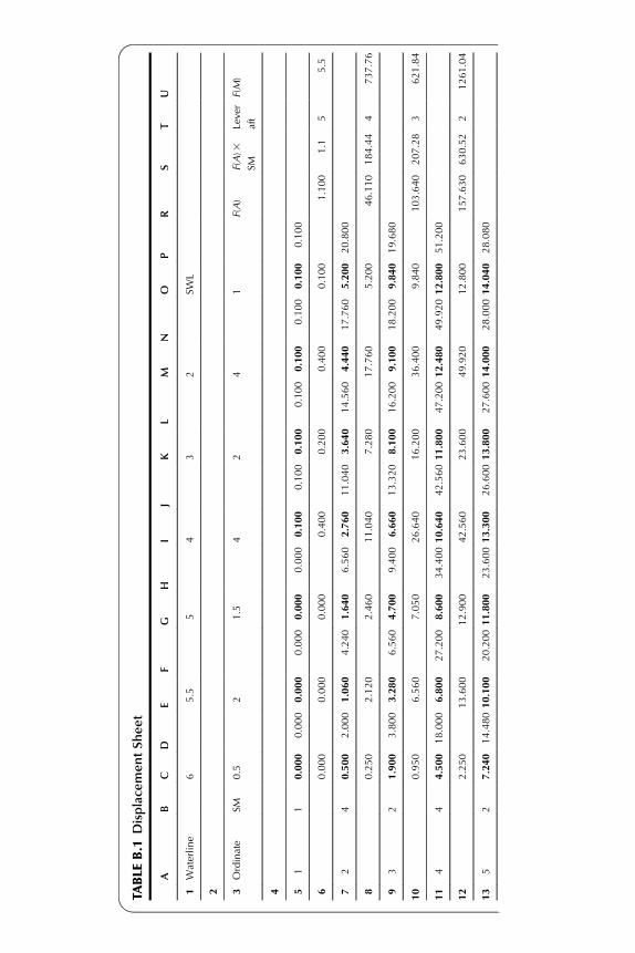
Table B.1 is a displacement sheet, using Microsoft Excel, for a vessel in
which the waterplanes are 2 m apart and the sections 14.1 m apart. The actual
half ordinates defining the underwater form of a body are shown in bold. For
greater definition in way of the turn of bilge, an intermediate waterplane has been
introduced between waterplanes 5 and 6, the Simpson’s multipliers being adjusted
accordingly. To simplify the arithmetic the appendages which would usually be
found below number 6, waterplane and aft of ordinate 11 have been ignored.
The figures in Row 6 are obtained from multiplying the half ordinates in
Row 5 by the corresponding Simpson’s multipliers in Row 3. Thus cell M6 is
the product of the contents of cells M3 and M5. Cell R6 is the sum of the cells
in Row 6 and represents the area of the section at ordinate 1 up to the summer
waterline (SWL). The figures in Column S are the result of multiplying the
figures in Column R by the Simpson’s multipliers in Column B. Cell S28 is
the sum of the figures in Column S and represents the volume of the immersed
body. The figures in Column U are the products of Columns S and T. Cell U28
is the sum of the figures in Column U and represents the moment of the
buoyancy force about amidships.
Correspondingly, the figure in cell D7 is the product of the figure in cell
C7 and the Simpson’s multiplier in cell B7. Then cell D28 is the sum of the
figures in Column D and represents the area of waterplane 6. The figures in
Row 30 are the result of multiplying the figures in Row 28 by the Simpson’s
multipliers in Row 3, noting that the SM for column D is that appearing in
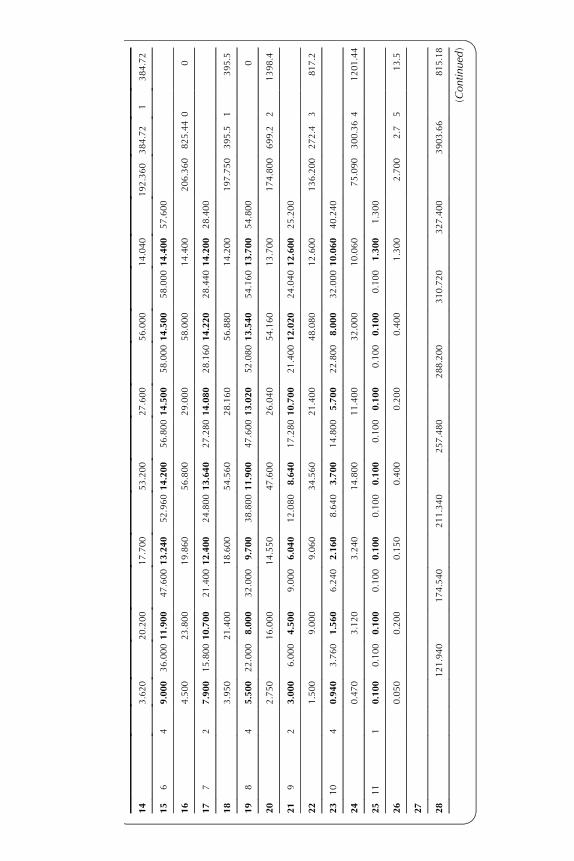
Column C, and so on. Cell R30 is the sum of the figures in Row 30 and
e1
TABLE
B.1
Displace
mentSheet
AB
CD
EF
GH
IJ
KL
MN
OP
RS
TU
1Waterline
65.5
54
32
SWL
2 3Ordinate
SM0.5
21.5
42
41
F(A)
F(A)3
SM
Lever
aft
F(M)
4 51
10.000
0.000
0.000
0.000
0.000
0.000
0.100
0.100
0.100
0.100
0.100
0.100
0.100
0.100
60.000
0.000
0.000
0.400
0.200
0.400
0.100
1.100
1.1
�5�5
.5
72
40.500
2.000
1.060
4.240
1.640
6.560
2.760
11.040
3.640
14.560
4.440
17.760
5.200
20.800
80.250
2.120
2.460
11.040
7.280
17.760
5.200
46.110
184.44�4
�737.76
93
21.900
3.800
3.280
6.560
4.700
9.400
6.660
13.320
8.100
16.200
9.100
18.200
9.840
19.680
10
0.950
6.560
7.050
26.640
16.200
36.400
9.840
103.640
207.28�3
�621.84
11
44
4.500
18.000
6.800
27.200
8.600
34.40010.640
42.56011.800
47.20012.480
49.92012.800
51.200
12
2.250
13.600
12.900
42.560
23.600
49.920
12.800
157.630
630.52�2
�1261.04
13
52
7.240
14.48010.100
20.20011.800
23.60013.300
26.60013.800
27.60014.000
28.00014.040
28.080
14
3.620
20.200
17.700
53.200
27.600
56.000
14.040
192.360
384.72
�1�3
84.72
15
64
9.000
36.00011.900
47.60013.240
52.96014.200
56.80014.500
58.00014.500
58.00014.400
57.600
16
4.500
23.800
19.860
56.800
29.000
58.000
14.400
206.360
825.440
0
17
72
7.900
15.80010.700
21.40012.400
24.80013.640
27.28014.080
28.16014.220
28.44014.200
28.400
18
3.950
21.400
18.600
54.560
28.160
56.880
14.200
197.750
395.5
1395.5
19
84
5.500
22.000
8.000
32.000
9.700
38.80011.900
47.60013.020
52.08013.540
54.16013.700
54.800
0
20
2.750
16.000
14.550
47.600
26.040
54.160
13.700
174.800
699.2
21398.4
21
92
3.000
6.000
4.500
9.000
6.040
12.080
8.640
17.28010.700
21.40012.020
24.04012.600
25.200
22
1.500
9.000
9.060
34.560
21.400
48.080
12.600
136.200
272.4
3817.2
23
10
40.940
3.760
1.560
6.240
2.160
8.640
3.700
14.800
5.700
22.800
8.000
32.00010.060
40.240
24
0.470
3.120
3.240
14.800
11.400
32.000
10.060
75.090
300.364
1201.44
25
11
10.100
0.100
0.100
0.100
0.100
0.100
0.100
0.100
0.100
0.100
0.100
0.100
1.300
1.300
26
0.050
0.200
0.150
0.400
0.200
0.400
1.300
2.700
2.7
513.5
27
28
121.940
174.540
211.340
257.480
288.200
310.720
327.400
3903.66
815.18
(Continued
)

TABLE
B.1
Displace
mentSheet—
(cont.)
AB
CD
EF
GH
IJ
KL
MN
OP
RS
TU
29
30
60.97
349.08
317.01
1029.92
576.4
1242.88
327.4
3903.66
31
Lever
54.5
43
21
0
32
33
Momen
t304.85
1570.86
1268.04
3089.76
1152.8
1242.88
08629.19
34
35
Volume
24463
36
Displacemen
t25075
37
LCBaft
2.94
38
VCB
5.58
39
40
represents the immersed volume of the body. Note: As a check on the
accuracy of the arithmetic, the figures in Cells S28 and R30 are the same
at 3903.66. The figures in Row 33 are obtained by multiplying the figures in
Row 30 by the corresponding levers in Row 31. Cell R33 is the sum of the
figures in Row 33 and represents the moment of buoyancy about the SWL.
Since the ordinates are for half the hull, the total hull volume is given by:
Volume5 23 (2/3)3 (14.1/3)3 3903.665 24,463 m3.
Displacement, in tonnes5 24,463(1.025)5 25,075 tonnes in seawater.
The centre of buoyancy of the hull from amidships5 14.1(815.18)/
(3903.66)5 2.94 m aft.
The centre of buoyancy below the SWL5 2(8629.19)/(3903.66) 5 4.42 m.
If wished these figures can be calculated within Excel and placed in
designated cells in the table.
Once a template has been created for the calculations, it can be used
repeatedly with new sets of ordinates. If one figure has to be changed in the
table, the computer will automatically correct all the related figures.
The computer naturally calculates figures to the full number of decimal
places. The number printed out can be controlled by the relevant command.
This should not lead the reader to suppose that the actual volume and centre
of buoyancy position have been calculated this accurately. For one thing, the
ordinates used will have limited accuracy and this will be compounded by
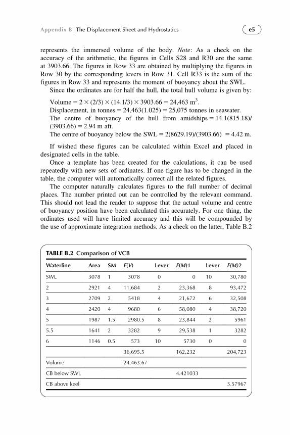
the use of approximate integration methods. As a check on the latter, Table B.2
TABLE B.2 Comparison of VCB
Waterline Area SM F(V) Lever F(M)1 Lever F(M)2
SWL 3078 1 3078 0 0 10 30,780
2 2921 4 11,684 2 23,368 8 93,472
3 2709 2 5418 4 21,672 6 32,508
4 2420 4 9680 6 58,080 4 38,720
5 1987 1.5 2980.5 8 23,844 2 5961
5.5 1641 2 3282 9 29,538 1 3282
6 1146 0.5 573 10 5730 0 0
36,695.5 162,232 204,723
Volume 24,463.67
CB below SWL 4.421033
CB above keel 5.57967
e5Appendix B|The Displacement Sheet and Hydrostatics

compares the vertical centre of buoyancy (VCB) position by taking moments
about the SWL and the keel. It will be noted that the two figures added together
correspond very closely to the draught of 10 m.
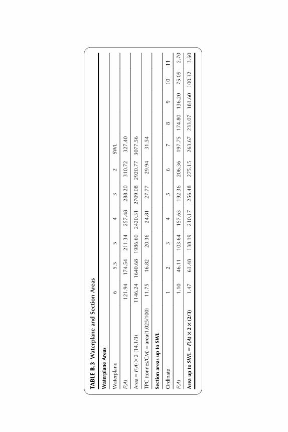
Waterplane and Section Areas
Embedded in Table B.1 are figures that can be used to derive the area of
each waterplane and the area of each section up to the SWL. The former are
in the second column of figures under each waterline (Columns D, F, H,
etc.); the latter in the second row against each ordinate (Rows 6, 8, 10, etc.).
These could be calculated within the main table, but for clarity of presenta-
tion they are here presented in Table B.3. The tonnes per centimetre immer-
sion are calculated for each waterplane.
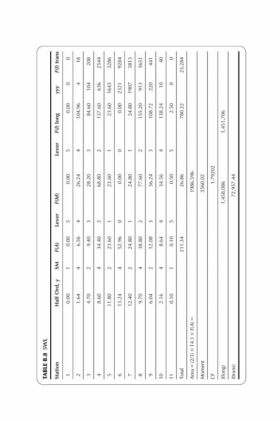
Tables can be produced for each waterplane, similar to Table 3.2 in
Chapter 3, to give the area, centroid position and the longitudinal and trans-
verse moments of inertia. These are presented in Tables B.4�B.10.
Note: In the row against I(long), the first figure is the moment of inertia
about amidships and the second is the inertia about the centre of flotation.
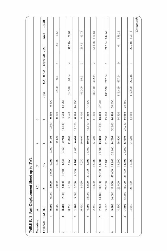
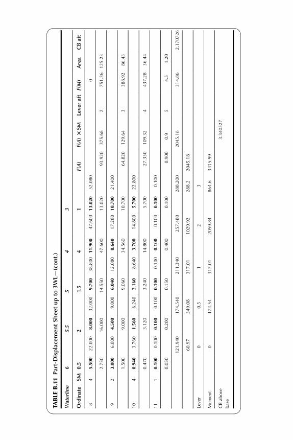
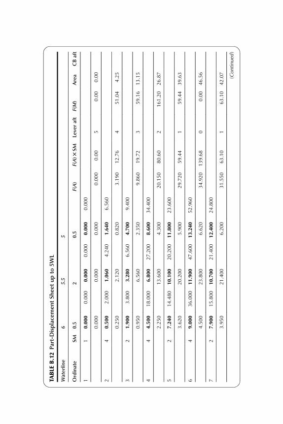
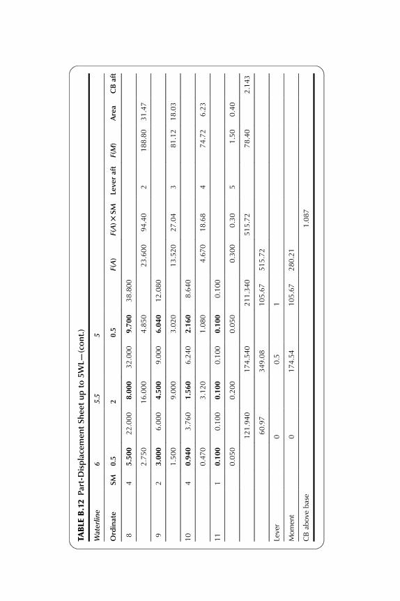
For the body up to 3WL and 5WL, part-displacement sheets can be
constructed as given in Tables B.11 and B.12, respectively.
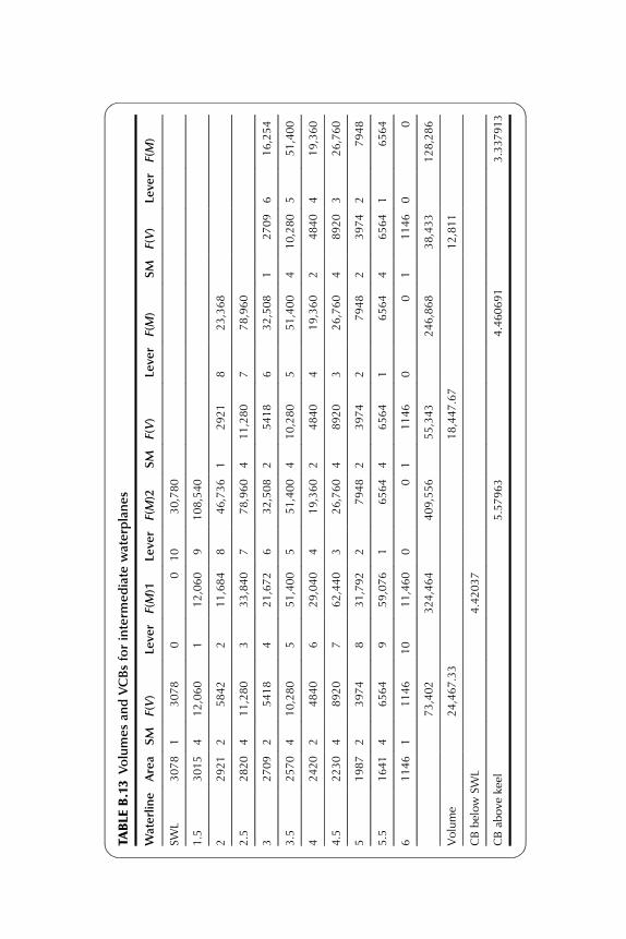
A convenient way of calculating the volume of displacement and VCB
position for waterlines 2 and 4 (as well as the SWL) is to plot the waterplane
areas to obtain the figures for intermediate waterplanes as given in
Table B.13.
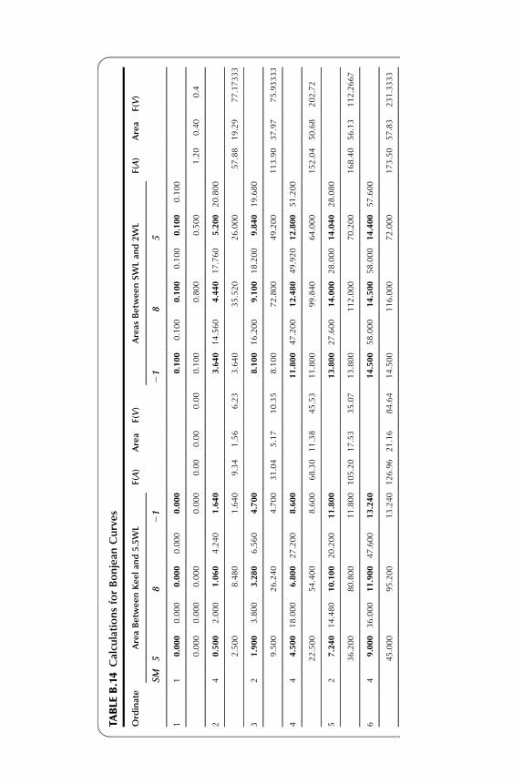
Bonjean Curves
The Bonjean curves can be calculated, for any section, by integration up to
each waterline in turn. The Simpson’s rule chosen in each case, and hence
the multiplying factor to be used, will depend upon the number of ordinates.
Table B.14 derives the section areas up to 5.5WL and between SWL and
2WL using Simpson’s 5, 8, 1 rule. Table B.15 derives the section areas
between the SWL and 4WL and 5WL using the 1, 3, 3, 1 rule and between
SWL and 5WL using the 1, 4, 21 rule. Then a table of cross-sectional areas
can be drawn up as given in Table B.16 from which the Bonjean curves can
be drawn. Figure B.1 uses the data given in Table B.16 to show the Bonjean
curves for ordinates 2, 3, 4 and 5.
Volumes and Longitudinal Centres of Buoyancy
The section areas can be used to calculate the volumes of displacement up to
each waterline and the corresponding longitudinal centres of buoyancy
(LCBs) as given in Table B.17.
e6 Introduction to Naval Architecture
TABLE
B.3
Waterplanean
dSectionAreas
WaterplaneAreas
Waterplane
65.5
54
32
SWL
F(A)
121.94
174.54
211.34
257.48
288.20
310.72
327.40
Area5F(A)3
2(14.1/3)
1146.24
1640.68
1986.60
2420.31
2709.08
2920.77
3077.56
TPC(tonnes/CM)5
area
(1.025/100)
11.75
16.82
20.36
24.81
27.77
29.94
31.54
Sectionarea
supto
SWL
Ordinate
12
34
56
78
910
11
F(A)
1.10
46.11
103.64
157.63
192.36
206.36
197.75
174.80
136.20
75.09
2.70
Areaupto
SWL5F(A)3
23(2/3)
1.47
61.48
138.19
210.17
256.48
275.15
263.67
233.07
181.60
100.12
3.60

TABLE
B.4
SW
L
Station
HalfOrd,y
SM
F(A)
Leve
rF(M)
Leve
rF(I)long
yyy
F(I)tran
s
10.10
10.10
50.50
52.50
00
25.20
420.80
483.20
4332.80
141
562
39.84
219.68
359.04
3177.12
953
1906
412.80
451.20
2102.40
2204.80
2097
8389
514.04
228.08
128.08
128.08
2768
5535
614.40
457.60
00.00
00.00
2986
11,944
714.20
228.40
�1�2
8.40
�128.40
2863
5727
813.70
454.80
�2�1
09.60
�2219.20
2571
10,285
912.60
225.20
�3�7
5.60
�3226.80
2000
4001
10
10.06
440.24
�4�1
60.96
�4643.84
1018
4072
11
1.30
11.30
�5�6
.50
�532.50
22
Total
327.40
�107.84
1896.04
52,423
Area5(2/3)3
14.13F(A)5
3077.56
Momen
t�1
4,293.1
Cen
treofflotation(CF)
�4.6443
I(long)
3,543,346
3,476,965
I(tran
s)16,4258.9

TABLE
B.5
2W
L
Station
HalfOrd,y
SM
F(A)
Leve
rF(M)
Leve
rF(I)long
yyy
F(I)tran
s
10.10
10.10
50.50
52.50
00
24.44
417.76
471.04
4284.16
88
350
39.10
218.20
354.60
3163.80
754
1507
412.48
449.92
299.84
2199.68
1944
7775
514.00
228.00
128.00
128.00
2744
5488
614.50
458.00
00.00
00.00
3049
12,195
714.22
228.44
�1�2
8.44
�128.44
2875
5751
813.54
454.16
�2�1
08.32
�2216.64
2482
9929
912.02
224.04
�3�7
2.12
�3216.36
1737
3473
10
8.00
432.00
�4�1
28.00
�4512.00
512
2048
11
0.10
10.10
�5�0
.50
�52.50
00
Total
310.72
�83.40
1654.08
48,516
Area5(2/3)3
14.13F(A)5
2920.768
Momen
t�1
1,053.8
CF
�3.78456
I(long)
3,091,168
3,049,334
I(tran
s)152,017.3

TABLE
B.6
3W
L
Station
HalfOrd,y
SM
F(A)
Leve
rF(M)
Leve
rF(I)long
yyy
F(I)tran
s
10.10
10.10
50.50
52.50
00
23.64
414.56
458.24
4232.96
48
193
38.10
216.20
348.60
3145.80
531
1063
411.80
447.20
294.40
2188.80
1643
6572
513.80
227.60
127.60
127.60
2628
5256
614.50
458.00
00.00
00.00
3049
12,195
714.08
228.16
�1�2
8.16
�128.16
2791
5583
813.02
452.08
�2�1
04.16
�2208.32
2207
8829
910.70
221.40
�3�6
4.20
�3192.60
1225
2450
10
5.70
422.80
�4�9
1.20
�4364.80
185
741
11
0.10
10.10
�5�0
.50
�52.50
00
Total
288.20
�58.88
1394.04
42,881
Area5(2/3)3
14.13F(A)5
2709.08
Momen
t�7
803.96
CF
�2.88067
I(long)
2,605,201
2,582,721
I(tran
s)134,359.4

TABLE
B.7
4W
L
Station
HalfOrd,y
SM
F(A)
Leve
rF(M)
Leve
rF(I)long
yyy
F(I)tran
s
10.10
10.10
50.50
52.50
00
22.76
411.04
444.16
4176.64
21
84
36.66
213.32
339.96
3119.88
295
591
410.64
442.56
285.12
2170.24
1205
4818
513.30
226.60
126.60
126.60
2353
4705
614.20
456.80
00.00
00.00
2863
11,453
713.64
227.28
�1�2
7.28
�127.28
2538
5075
811.90
447.60
�2�9
5.20
�2190.40
1685
6741
98.64
217.28
�3�5
1.84
�3155.52
645
1290
10
3.70
414.80
�4�5
9.20
�4236.80
51
203
11
0.10
10.10
�5�0
.50
�52.50
00
Total
257.48
�37.68
1108.36
34,960
Area5(2/3)3
14.13F(A)5
2420.312
Momen
t�4
994.11
CF
�2.06341
I(long)
2,071,319
2,061,014
I(tran
s)109,541.9
TABLE
B.8
5W
L
Station
HalfOrd,y
SM
F(A)
Leve
rF(M)
Leve
rF(I)long
yyy
F(I)tran
s
10.00
10.00
50.00
50.00
00
21.64
46.56
426.24
4104.96
418
34.70
29.40
328.20
384.60
104
208
48.60
434.40
268.80
2137.60
636
2544
511.80
223.60
123.60
123.60
1643
3286
613.24
452.96
00.00
00.00
2321
9284
712.40
224.80
�1�2
4.80
�124.80
1907
3813
89.70
438.80
�2�7
7.60
�2155.20
913
3651
96.04
212.08
�3�3
6.24
�3108.72
220
441
10
2.16
48.64
�4�3
4.56
�4138.24
10
40
11
0.10
10.10
�5�0
.50
�52.50
00
Total
211.34
�26.86
780.22
23,284
Area5(2/3)3
14.13F(A)5
1986.596
Momen
t�3
560.02
CF
�1.79202
I(long)
1,458,086
1,451,706
I(tran
s)72,957.44

TABLE
B.9
5.5W
L
Station
HalfOrd,y
SM
F(A)
Leve
rF(M)
Leve
rF(I)long
yyy
F(I)tran
s
10.00
10.00
50.00
50.00
00
21.06
44.24
416.96
467.84
15
33.28
26.56
319.68
359.04
35
71
46.80
427.20
254.40
2108.80
314
1258
510.10
220.20
120.20
120.20
1030
2061
611.90
447.60
00.00
00.00
1685
6741
710.70
221.40
�1�2
1.40
�121.40
1225
2450
88.00
432.00
�2�6
4.00
�2128.00
512
2048
94.50
29.00
�3�2
7.00
�381.00
91
182
10
1.56
46.24
�4�2
4.96
�499.84
415
11
0.10
10.10
�5�0
.50
�52.50
00
Total
174.54
�26.62
588.62
14,830
Area5(2/3)3
14.13F(A)5
1640.676
Momen
t�3
528.21
CF
�2.15046
I(long)
1,100,021
1,092,434
I(tran
s)46,466.79

TABLE
B.10
6W
L
Station
HalfOrd,y
SM
F(A)
Leve
rF(M)
Leve
rF(I)long
yyy
F(I)tran
s
10.00
10.00
50.00
50.00
00
20.50
42.00
48.00
432.00
01
31.90
23.80
311.40
334.20
714
44.50
418.00
236.00
272.00
91
365
57.24
214.48
114.48
114.48
380
759
69.00
436.00
00.00
00.00
729
2916
77.90
215.80
�1�1
5.80
�115.80
493
986
85.50
422.00
�2�4
4.00
�288.00
166
666
93.00
26.00
�3�1
8.00
�354.00
27
54
10
0.94
43.76
�4�1
5.04
�460.16
13
11
0.10
10.10
�5�0
.50
�52.50
00
Total
121.94
�23.46
373.14
5763
Area5(2/3)3
14.13F(A)5
1146.236
Momen
t�3
109.39
CF
�2.71269
I(long)
697,329.3
688,894.4
I(tran
s)18,056.23
TABLE
B.11Part-Displace
mentSheetupto
3W
L
Waterline
65.5
54
3
Ordinate
SM
0.5
21.5
41
F(A)
F(A)3SM
Leve
raft
F(M)
Area
CBaft
11
0.000
0.000
0.000
0.000
0.000
0.000
0.100
0.100
0.100
0.100
0.000
0.000
0.000
0.400
0.100
0.500
0.5
�5�2
.50.67
24
0.500
2.000
1.060
4.240
1.640
6.560
2.760
11.040
3.640
14.560
0.250
2.120
2.460
11.040
3.640
19.510
78.04
�4�3
12.16
26.01
32
1.900
3.800
3.280
6.560
4.700
9.400
6.660
13.320
8.100
16.200
0.950
6.560
7.050
26.640
8.100
49.300
98.6
�3�2
95.8
65.73
44
4.500
18.000
6.800
27.200
8.600
34.400
10.640
42.560
11.800
47.200
2.250
13.600
12.900
42.560
11.800
83.110
332.44
�2�6
64.88
110.81
52
7.240
14.480
10.100
20.200
11.800
23.600
13.300
26.600
13.800
27.600
3.620
20.200
17.700
53.200
13.800
108.520
217.04
�1�2
17.04
144.69
64
9.000
36.000
11.900
47.600
13.240
52.960
14.200
56.800
14.500
58.000
4.500
23.800
19.860
56.800
14.500
119.460
477.84
00
159.28
72
7.900
15.800
10.700
21.400
12.400
24.800
13.640
27.280
14.080
28.160
3.950
21.400
18.600
54.560
14.080
112.590
225.18
1225.18
150.12 (Continued
)
TABLE
B.11Part-Displace
mentSheetupto
3W
L—(cont.)
Waterline
65.5
54
3
Ordinate
SM
0.5
21.5
41
F(A)
F(A)3SM
Leve
raft
F(M)
Area
CBaft
84
5.500
22.000
8.000
32.000
9.700
38.800
11.900
47.600
13.020
52.080
0
2.750
16.000
14.550
47.600
13.020
93.920
375.68
2751.36
125.23
92
3.000
6.000
4.500
9.000
6.040
12.080
8.640
17.280
10.700
21.400
1.500
9.000
9.060
34.560
10.700
64.820
129.64
3388.92
86.43
10
40.940
3.760
1.560
6.240
2.160
8.640
3.700
14.800
5.700
22.800
0.470
3.120
3.240
14.800
5.700
27.330
109.32
4437.28
36.44
11
10.100
0.100
0.100
0.100
0.100
0.100
0.100
0.100
0.100
0.100
0.050
0.200
0.150
0.400
0.100
0.900
0.9
54.5
1.20
121.940
174.540
211.340
257.480
288.200
2045.18
314.86
2.170726
60.97
349.08
317.01
1029.92
288.2
2045.18
Lever
00.5
12
3
Momen
t0
174.54
317.01
2059.84
864.6
3415.99
CBab
ove
base
3.340527
TABLE
B.12
Part-Displace
mentSheetupto
5W
L
Waterline
65.5
5
Ordinate
SM
0.5
20.5
F(A)
F(A)3
SM
Leve
raft
F(M)
Area
CBaft
11
0.000
0.000
0.000
0.000
0.000
0.000
0.000
0.000
0.000
0.000
0.00
�50.00
0.00
24
0.500
2.000
1.060
4.240
1.640
6.560
0.250
2.120
0.820
3.190
12.76
�4�5
1.04
4.25
32
1.900
3.800
3.280
6.560
4.700
9.400
0.950
6.560
2.350
9.860
19.72
�3�5
9.16
13.15
44
4.500
18.000
6.800
27.200
8.600
34.400
2.250
13.600
4.300
20.150
80.60
�2�1
61.20
26.87
52
7.240
14.480
10.100
20.200
11.800
23.600
3.620
20.200
5.900
29.720
59.44
�1�5
9.44
39.63
64
9.000
36.000
11.900
47.600
13.240
52.960
4.500
23.800
6.620
34.920
139.68
00.00
46.56
72
7.900
15.800
10.700
21.400
12.400
24.800
3.950
21.400
6.200
31.550
63.10
163.10
42.07
(Continued
)
TABLE
B.12
Part-Displace
mentSheetupto
5W
L—(cont.)
Waterline
65.5
5
Ordinate
SM
0.5
20.5
F(A)
F(A)3
SM
Leve
raft
F(M)
Area
CBaft
84
5.500
22.000
8.000
32.000
9.700
38.800
2.750
16.000
4.850
23.600
94.40
2188.80
31.47
92
3.000
6.000
4.500
9.000
6.040
12.080
1.500
9.000
3.020
13.520
27.04
381.12
18.03
10
40.940
3.760
1.560
6.240
2.160
8.640
0.470
3.120
1.080
4.670
18.68
474.72
6.23
11
10.100
0.100
0.100
0.100
0.100
0.100
0.050
0.200
0.050
0.300
0.30
51.50
0.40
121.940
174.540
211.340
515.72
78.40
2.143
60.97
349.08
105.67
515.72
Lever
00.5
1
Momen
t0
174.54
105.67
280.21
CBab
ove
base
1.087
TABLE
B.13
Volumesan
dVCBsforinterm
ediate
waterplanes
Waterline
Area
SM
F(V)
Leve
rF(M)1
Leve
rF(M)2
SM
F(V)
Leve
rF(M)
SM
F(V)
Leve
rF(M)
SWL
3078
13078
00
10
30,780
1.5
3015
412,060
112,060
9108,540
22921
25842
211,684
846,736
12921
823,368
2.5
2820
411,280
333,840
778,960
411,280
778,960
32709
25418
421,672
632,508
25418
632,508
12709
616,254
3.5
2570
410,280
551,400
551,400
410,280
551,400
410,280
551,400
42420
24840
629,040
419,360
24840
419,360
24840
419,360
4.5
2230
48920
762,440
326,760
48920
326,760
48920
326,760
51987
23974
831,792
27948
23974
27948
23974
27948
5.5
1641
46564
959,076
16564
46564
16564
46564
16564
61146
11146
10
11,460
00
11146
00
11146
00
73,402
324,464
409,556
55,343
246,868
38,433
128,286
Volume
24,467.33
18,447.67
12,811
CBbelow
SWL
4.42037
CBab
ove
keel
5.57963
4.460691
3.337913
TABLE
B.14Calcu
lationsforBonjean
Curves
Ordinate
AreaBetw
eenKeelan
d5.5WL
F(A)
Area
F(V)
Areas
Betw
eenSWLan
d2WL
F(A)
Area
F(V)
SM
58
21
21
85
11
0.000
0.000
0.000
0.000
0.000
0.100
0.100
0.100
0.100
0.100
0.100
0.000
0.000
0.000
0.000
0.00
0.00
0.00
�0.100
0.800
0.500
1.20
0.40
0.4
24
0.500
2.000
1.060
4.240
1.640
3.640
14.560
4.440
17.760
5.200
20.800
2.500
8.480
�1.640
9.34
1.56
6.23
�3.640
35.520
26.000
57.88
19.29
77.17333
32
1.900
3.800
3.280
6.560
4.700
8.100
16.200
9.100
18.200
9.840
19.680
9.500
26.240
�4.700
31.04
5.17
10.35
�8.100
72.800
49.200
113.90
37.97
75.93333
44
4.500
18.000
6.800
27.200
8.600
11.800
47.200
12.480
49.920
12.800
51.200
22.500
54.400
�8.600
68.30
11.38
45.53
�11.800
99.840
64.000
152.04
50.68
202.72
52
7.240
14.480
10.100
20.200
11.800
13.800
27.600
14.000
28.000
14.040
28.080
36.200
80.800
�11.800
105.20
17.53
35.07
�13.800
112.000
70.200
168.40
56.13
112.2667
64
9.000
36.000
11.900
47.600
13.240
14.500
58.000
14.500
58.000
14.400
57.600
45.000
95.200
�13.240
126.96
21.16
84.64
�14.500
116.000
72.000
173.50
57.83
231.3333

72
7.900
15.800
10.700
21.400
12.400
14.080
28.160
14.220
28.440
14.200
28.400
39.500
85.600
�12.400
112.70
18.78
37.57
�14.080
113.760
71.000
170.68
56.89
113.7867
84
5.500
22.000
8.000
32.000
9.700
13.020
52.080
13.540
54.160
13.700
54.800
27.500
64.000
�9.700
81.80
13.63
54.53
�13.020
108.320
68.500
163.80
54.60
218.4
92
3.000
6.000
4.500
9.000
6.040
10.700
21.400
12.020
24.040
12.600
25.200
15.000
36.000
�6.040
44.96
7.49
14.99
�10.700
96.160
63.000
148.46
49.49
98.97333
10
40.940
3.760
1.560
6.240
2.160
5.700
22.800
8.000
32.000
10.060
40.240
4.700
12.480
�2.160
15.02
2.50
10.01
�5.700
64.000
50.300
108.60
36.20
144.8
11
10.100
0.100
0.100
0.100
0.100
0.100
0.100
0.100
0.100
1.300
1.300
0.500
0.800
�0.100
1.20
0.20
0.20
�0.100
0.800
6.500
7.20
2.40
2.4
F(V)
299.11
1278.187
Volume
1405.83
6007.48

TABLE
B.15
SectionAreas
Betw
eenSW
Lan
d4W
Lan
d5W
L
54
32
SW
L
WL
SM
14
24
1F(A)
F(A)
Ordinate
SM
13
31
(4W
L)(5W
L)Area(5)
Area(4)
11
0.00
0.00
0.10
0.10
0.10
0.10
0.10
0.10
0.10
0.10
0.00
0.40
0.20
0.40
0.10
1.10
1.47
0.10
0.30
0.30
0.10
0.80
1.20
24
1.64
6.56
2.76
11.04
3.64
14.56
4.44
17.76
5.20
20.80
1.64
11.04
7.28
17.76
5.20
42.92
57.23
2.76
10.92
13.32
5.20
32.20
48.30
32
4.70
9.40
6.66
13.32
8.10
16.20
9.10
18.20
9.84
19.68
4.70
26.64
16.20
36.40
9.84
93.78
125.04
6.66
24.30
27.30
9.84
68.10
102.15
44
8.60
34.40
10.64
42.56
11.80
47.20
12.48
49.92
12.80
51.20
8.60
42.56
23.60
49.92
12.80
137.48
183.31
10.64
35.40
37.44
12.80
96.28
144.42
52
11.80
23.60
13.30
26.60
13.80
27.60
14.00
28.00
14.04
28.08
11.80
53.20
27.60
56.00
14.04
162.64
216.85
13.30
41.40
42.00
14.04
110.74
166.11
64
13.24
52.96
14.20
56.80
14.50
58.00
14.50
58.00
14.40
57.60
13.24
56.80
29.00
58.00
14.40
171.44
228.59
14.20
43.50
43.50
1.0
14.40
115.60
173.40
72
12.40
24.80
13.64
27.28
14.08
28.16
14.22
28.44
14.20
28.40
12.40
54.56
28.16
56.88
14.20
166.20
221.60
13.64
42.24
42.66
14.20
112.74
169.11
84
9.70
38.80
11.90
47.60
13.02
52.08
13.54
54.16
13.70
54.80
9.70
47.60
26.04
54.16
13.70
151.20
201.60
11.90
39.06
40.62
13.70
105.28
157.92
92
6.04
12.08
8.64
17.28
10.70
21.40
12.02
24.04
12.60
25.20
6.04
34.56
21.40
48.08
12.60
122.68
163.57
8.64
32.10
36.06
12.60
89.40
134.10
10
42.16
8.64
3.70
14.80
5.70
22.80
8.00
32.00
10.06
40.24
2.16
14.80
11.40
32.00
10.06
70.42
93.89
3.70
17.10
24.00
10.06
54.86
82.29
11
10.10
0.10
0.10
0.10
0.10
0.10
0.10
0.10
1.30
1.30
0.10
0.40
0.20
0.40
1.30
2.40
3.20
0.10
0.30
0.30
0.10
1.30
2.00
3.00
Areato
5WL5F(A)(5WL)3232/3
5(4/3)F(A)(5WL).
Areato
4WL5F(A)(4WL)32323(3/8)5
1.5F(A)(4WL).

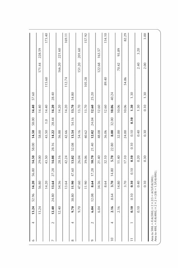
TABLE B.16 Table of Section Areas
Ord Area to
6WL 5.5WL 5WL 4WL 3WL 2WL SWL
1 0.00 0.00 0.00 0.27 0.67 1.07 1.47
2 0.00 1.56 4.25 13.18 26.01 42.19 61.48
3 0.00 5.17 13.15 36.04 65.73 100.22 138.19
4 0.00 11.38 26.87 65.75 110.81 159.49 210.17
5 0.00 17.53 39.63 90.37 144.69 200.35 256.48
6 0.00 21.16 46.56 101.75 159.28 217.32 275.15
7 0.00 18.78 42.07 94.56 150.12 206.78 263.67
8 0.00 13.63 31.47 75.15 125.23 178.47 233.07
9 0.00 7.49 18.03 47.50 86.43 132.11 181.60
10 0.00 2.50 6.23 17.83 36.44 63.92 100.12
11 0.00 0.20 0.40 0.60 1.20 1.60 3.60
10Sect 2
Dra
ught
Sect 3 Sect 4 Sect 5
8
6
4
2
50 100 150 200 250
Area (m2)
FIGURE B.1 Bonjean curves.
e24 Introduction to Naval Architecture

TABLE
B.17
Volumesan
dLC
Bs
Ord
SM
Leve
rAreato
5.5WL
5WL
Area
F(V)
F(M)
Area
F(V)
F(M)
11
50.00
0.00
0.00
0.00
0.00
0.00
24
41.56
6.24
24.96
4.25
17.00
68.00
32
35.17
10.34
31.02
13.15
26.30
78.90
44
211.38
45.52
91.04
26.87
107.48
214.96
52
117.53
35.06
35.06
39.63
79.26
79.26
64
021.16
84.64
0.00
46.56
186.24
0.00
72
21
18.78
37.56
237.56
42.07
84.14
284.14
84
22
13.63
54.52
2109.04
31.47
125.88
2251.76
92
23
7.49
14.98
244.94
17.53
35.06
2105.18
10
424
2.50
10.00
240.00
6.23
24.92
299.68
11
125
0.20
0.20
21.00
0.40
0.40
22.00
Total
99.40
299.06
250.46
686.68
2101.64
Volume
CBaft
1405.582
22.379074
3227.396
22.087033
Displace
men
t1440.722
3308.081
(Continued
)

TABLE
B.17
Volumesan
dLC
Bs—
(cont.)
Ord
SM
Leve
r4WL
3WL
Area
F(V)
F(M)
Area
F(V)
F(M)
11
50.27
0.27
1.35
0.67
0.67
3.35
24
413.18
52.72
210.88
26.01
104.04
416.16
32
336.04
72.08
216.24
65.73
131.46
394.38
44
265.75
263.00
526.00
110.81
443.24
886.48
52
190.37
180.74
180.74
144.69
289.38
289.38
64
0101.75
407.00
0.00
159.28
637.12
0.00
72
21
94.56
189.12
2189.12
150.12
300.24
2300.24
84
22
75.15
300.60
2601.20
125.23
500.92
21001.84
92
23
47.50
95.00
2285.00
86.43
172.86
2518.58
10
424
17.83
71.32
2285.28
36.44
145.76
2583.04
11
125
0.60
0.60
23.00
1.20
1.20
26.00
Total
1632.45
2228.39
2726.89
2419.95
Volume
CBaft
7672.515
21.972678
12,816.38
22.171446
Displace
men
t7864.328
13,136.79

Ord
SM
Leve
r2WL
SWL
Area
F(V)
F(M)
Area
F(V)
F(M)
11
51.07
1.07
5.35
1.47
1.47
7.35
24
442.19
168.76
675.04
61.48
245.92
983.68
32
3100.22
200.44
601.32
138.19
276.38
829.14
44
2159.49
637.96
1275.92
210.17
840.68
1681.36
52
1200.35
400.70
400.70
256.48
512.96
512.96
64
0217.32
869.28
0.00
275.15
1100.60
0.00
72
21
206.78
413.56
2413.56
263.67
527.34
2527.34
84
22
178.47
713.88
21427.76
233.07
932.28
21864.56
92
23
132.11
264.22
2792.66
181.60
363.20
21089.60
10
424
63.92
255.68
21022.72
100.12
400.48
21601.92
11
125
1.60
1.60
28.00
3.60
3.60
218.00
Total
3927.15
2706.37
5204.91
21086.93
Volume
CBaft
18,457.61
22.536144
24,463.08
22.944472
Displace
men
t18,919.05
25,074.65

TABLE
B.18
KBan
dKM
Values
WL
65.5
54
32
SW
L
TransI
18,056
46,467
72,957
109,542
134,359
152,017
164,259
Volume,
V0
1406
3232
7505
12,816
18,470
24,463
TransBM
33.05
22.57
14.60
10.48
8.23
6.71
KB
00.53
1.09
2.22
3.34
4.46
5.58
TransKM
33.58
23.66
16.82
13.82
12.69
12.29
LongI
688,900
1,092,400
1,451,700
2,061,000
258,700
3,049,300
3,477,000
LongBM
777
449
275
202
165
142
LongKM
777
450
277
205
170
148
Additional
dataforplottinghyd
rostatic
curves
Massdisplacemen
t0
1441
3313
7693
13,136
18,932
25,075
TPC
11.75
16.82
20.36
24.81
27.77
29.94
31.54
CFaft
2.71
2.15
1.79
2.06
2.88
3.78
4.64
LCBaft
2.38
2.09
1.97
2.17
2.54
2.94
Further
ifKG511m
LongGM
766
439
266
194
159
137
MCT
7830
10,320
14,510
18,070
21,350
24,360
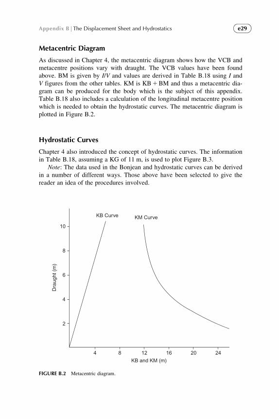
Metacentric Diagram
As discussed in Chapter 4, the metacentric diagram shows how the VCB and
metacentre positions vary with draught. The VCB values have been found
above. BM is given by I/V and values are derived in Table B.18 using I and
V figures from the other tables. KM is KB1BM and thus a metacentric dia-
gram can be produced for the body which is the subject of this appendix.
Table B.18 also includes a calculation of the longitudinal metacentre position
which is needed to obtain the hydrostatic curves. The metacentric diagram is
plotted in Figure B.2.
Hydrostatic Curves
Chapter 4 also introduced the concept of hydrostatic curves. The information
in Table B.18, assuming a KG of 11 m, is used to plot Figure B.3.
Note: The data used in the Bonjean and hydrostatic curves can be derived
in a number of different ways. Those above have been selected to give the
reader an idea of the procedures involved.
KB Curve
Dra
ught
(m
)
KB and KM (m)
KM Curve
10
8
6
4
2
4 8 12 16 20 24
FIGURE B.2 Metacentric diagram.
e29Appendix B|The Displacement Sheet and Hydrostatics

10
8
6
Dra
ught
(m
)
Disp.
CF
LCB
TPCM
CT
4
2
5 000
5 000
5 10 15 20 25 30
654321
1 2 3 4 5 6
10 000
10 000
15 000
15 000
20 000
20 000
25 000
25 000
30 000
30 000
Disp. (tonnes)
TPC (tonnes/cm)
CF aft of (m)
LCB aft of (m)
MCT (tonnes.m/m)
FIGURE B.3 Hydrostatic curves.
e30 Introduction to Naval Architecture