sectoral effects of ringgit depreciation … effects of ringgit depreciation shocks 137 export...
TRANSCRIPT
JOURNAL OF ECONOMIC DEVELOPMENT 135 Volume 32, Number 2, December 2007
SECTORAL EFFECTS OF RINGGIT DEPRECIATION SHOCKS
MANSOR H. IBRAHIM∗
International Islamic University Malaysia
The paper seeks to address two important questions-namely, is exchange rate depreciation expansionary or contractionary and are there distributional consequences of exchange rate shocks for the case of Malaysia? In the paper, we consider the relations between aggregate output as well as eight sectoral outputs and real effective exchange rate in multivariate setting. Applying multivariate cointegration test, we find evidence for cointegration among the variables for all sectors. More importantly, both real output (aggregate output as well as all sectoral output) and real exchange rate contribute significantly to the cointegration space, affirming the presence of long run relations between the two focused variables. In most cases, the estimated cointegrating vectors suggest expansionary currency depreciation. Our simulated dynamics using generalized impulse responses further substantiate this finding especially over longer horizons. Over shorter horizons, however, exchange rate depreciation can be contractionary for certain sectors particularly for the construction sector. Lastly, we also find evidence indicative of the differential effects of the currency shocks. Comparatively, the manufacturing sector, transport, storage and communication sector, and finance, insurance, real estates and business services sector seem to be affected more by exchange rate fluctuations. Keywords: Exchange Rate Shocks, Sectoral Output, Cointegration, Generalized
Impulse Responses JEL classification: F31
1. INTRODUCTION The dramatic swings in the currency values since the breakdown of the Bretton
Woods System have continued to stir interest in the effects of currency depreciation on macroeconomic performance. For Malaysia and other East-Asian countries, the interest in the subject is further heightened by the eruption of the Asian crisis in July 1997. These countries witnessed drastic drop in their currency values which then reverberated ∗ I would like to express my thanks to the anonymous referee and the editor of the Journal for helpful comments. I am, however, responsible for the remaining errors.

MANSOR H. IBRAHIM 136
throughout various sectors of the economy including the real sector. At its depth in 1998, all crisis-hit countries experienced drastic drop in their economic growth. In 1997, the growth rates of Indonesia, South Korea, Malaysia, the Philippines, and Thailand were respectively 4.7%, 5.0%, 7.3%, 5.2% and -1.7%. Then, in 1998, these figures dropped substantially to -13.1% (Indonesia), -6.7% (South Korea), -7.4% (Malaysia), -0.6% (the Philippines), and -10.2% (Thailand). Moreover, different sectors in the economy seem to be affected differently. In the case of Malaysia, the construction sector experienced the biggest contraction of its real output followed by the manufacturing sector. Indeed, the contraction of 7.4% in Malaysian real GDP in 1998 was accounted mostly by these two sectors, where output from the construction and manufacturing sectors dropped by 23% and 13% respectively.
The experience of the crisis, starting with currency depreciation shocks and culminating in the worst recession ever for crisis-hit economies, reinforces a recent view that exchange rate depreciation is harmful to the economy. However, countering this view, we may also argue that the contractionary effect of currency depreciation as noted during the crisis is special only to the event of the crisis magnitude. In other words, the question as to whether currency depreciation depresses or encourages output during non-crisis period is still open. Indeed, some developing countries still pursue devaluation policies as a way to expand real production due to the belief that currency depreciation is expansionary.
Apart from this issue, the Asian crisis also brings into the surface distributional consequences of currency shocks, an important issue for a country like Malaysia that seeks to achieve high economic growth together with equal distribution of income. Accordingly, in view of the recent effects of the Asian currency crisis, the following questions are highly relevant: Is currency depreciation contractionary or expansionary? Does currency depreciation affect different sectors differently? The present paper seeks to answer these two questions for the case of Malaysia. Our main analysis relies on historical data prior to the crisis. Then, as a further analysis, we extend the observations beyond the Asian crisis period to assess whether the Asian crisis has disrupted the relations between real activities and exchange rate1. This extension also allows us to assess the robustness of our results.
Since independence, Malaysia has observed the rising importance of the international trade. In 1980, the ratio of Malaysian exports of goods and services to GDP was 0.58. This ratio increased steadily to 0.81 in 1990 and reached 0.94 in 1997. The continuous increase in the export ratio has been accompanied by the changes in the
1 We thank the anonymous referee for giving this suggestion. Ideally, we should evaluate the exchange rate - real output relationships for the period before the crisis and for the period after the crisis separately to see if there are structural changes. For this to be possible, we need sufficient observations for the post-crisis period. However, sufficient data for post-crisis period are yet available. Accordingly, our results for the extended sample should be viewed as exploratory.
SECTORAL EFFECTS OF RINGGIT DEPRECIATION SHOCKS 137
export structures. Originally, Malaysia exported mainly commodities such as tin and rubber to the world markets. However, with the shift in emphasis toward industrialization, manufactured goods have now been the main exports of Malaysia. At the same time, Malaysia is also highly dependent on imported goods for its production, which stems mainly from the industrialization orientation of the country. The ratio of imported investment and intermediate goods has been well over 80% since 1980. This open nature of the Malaysian economy makes Malaysia an interesting case study as it is expected to be highly susceptible to currency shocks. The noted Asian crisis that hit the country further adds importance of the issue to the Malaysian case.
The rest of the paper is organized as follows. In the next section, we review existing literature, looking at both theories and empirical evidence on the issue. Section 3 describes the empirical approach taken by the study. Section 4 presents estimation results and, finally, section 5 concludes with the main findings.
2. LITERATURE REVIEW Economic theories acknowledge both positive and negative effects of currency
depreciation on real output. An early dominant view emphasizes expansionary effects of currency depreciation. Specifically, exchange rate depreciation makes a country’s exports cheaper in the global markets. This will stimulate domestic aggregate demand and increase real GDP. Recently, however, some have made a case for the possibility that exchange rate depreciation may adversely affect real output and, accordingly, nullifies its noted benefits on the country’s exports. There is also a view that the exchange rate and real output may not be related. The observed relation between them may be driven by the third common factor such as productivity or monetary policy.
The negative effect of exchange rate depreciation is viewed highly possible for developing countries. A main channel stressed in the literature that accounts for contractionary depreciation works through the supply side of the economy by affecting the costs of production inputs (Krugman and Taylor (1976) and Edwards (1986)). Normally, developing countries depend greatly on imported inputs for their production process. Currency depreciation increases the costs of domestic production by raising the costs of imported inputs. This increase in the production costs shifts the aggregate supply inwards, resulting in contraction of real output. Apart from this supply-side effect, it is also conceivable that exchange rate depreciation can retard aggregate demand of the economy, contradicting the conventional view. Edwards (1986) and Upadhyaya (1999) highlight three possible negative aggregate demand effects of currency changes. These include real balance effect, income distribution effect and trade balance effect.
Underlying real balance effect is the contention that exchange rate depreciation raises aggregate price level. As prices rise, real money balances decline leading to contraction in aggregate demand. The income distribution effect rests on the argument that different classes of consumers may have different marginal propensities to consume.

MANSOR H. IBRAHIM 138
For example, the marginal propensity to consume of workers may be higher than that of capital owners. According to this channel, currency depreciation tends to redistribute income from classes of consumers that have a high marginal propensity to consume to the classes that have a low marginal propensity to consume. As a result, aggregate consumption may drop. Lastly, the positive effect of currency depreciation on trade balance depends in part on the Marshall-Lerner condition that the sum of price elasticity of demand for exports and price elasticity of demand for imports is greater than unity. However, if these elasticities are sufficiently low, the trade balance in domestic terms may be adversely affected. Accordingly, currency depreciation can be recessionary.
While these views suggest either positive or negative effects of currency depreciation, Tatom (1987, 1988) raises the possibility that the change in the exchange rate is the symptom or the result of a strong economic performance. To him, the influence of the exchange rate on real activity would be appropriate only if the change in the exchange rates is exogenous. However, domestic economic policies aiming at improving a country’s output and productivity may, at the same time, influence the country’s currency value. From this view, we may discern two alternative patterns in the real output-exchange rate linkages. Along the line suggested by Tatom (1987, 1988), an increase in real output and productivity may strengthen the currency value, suggesting causation that flows from real output to exchange rate. Alternatively, the currency value and real output may not be related. Any observed relation is spurious as it may be driven by common factors such as productivity changes and monetary policies.
These contradicting views have inspired enormous empirical research that seeks to pinpoint the impacts of currency depreciation especially for the case of developing countries. Among early empirical studies on the output effect of exchange rate changes include those by Gylfason and Schmid (1983), Connolly (1983), Gylfason and Risager (1984), Edwards (1986), Solimano (1986), and Gylfason and Radetzki (1991). Evaluating the effects of devaluation for 10 developed and developing countries, Gylfason and Schmid (1983) find evidence for the expansionary effects of devaluation in 8 countries. Connolly (1983) provides further support for the expansionary devaluation in a group of 22 countries. Gylfason and Risager (1984) also document some evidence for the positive effects of the reduction in the currency’s value in developed countries. However, they note that, in developing countries, currency devaluation tends to exert a negative influence on output. Evaluating the issue for 12 developing countries, Edwards (1986) also find some support for the hypothesis of contractionary devaluation in the short run. However, he finds devaluation to be neutral in the long run. Solimano (1986) also provides evidence for contractionary devaluation for the case of Chile. Recently, Gylfason and Radetzki (1991) attempt to evaluate the issue by focusing on 12 least developing countries. They further note the evidence that devaluation has a negative effect on output.
While these studies have provided an interesting ground for empirical debate, they are noted to have at least two main weaknesses. First, as argued by Tatom (1987, 1988), the exchange rate may well be endogenous responding to the underlying economic
SECTORAL EFFECTS OF RINGGIT DEPRECIATION SHOCKS 139
conditions including real economic activity. However, the existing analyses using structural models fail to take this into consideration. And second, since the seminal work of Nelson and Plosser (1982), it is now recognized that most macroeconomic series are non-stationary. Then, as noted by Engle and Granger (1987), a set of non-stationary variables may be cointegrated or share a long run equilibrium path. Failing to take these univariate and multivariate properties of the time series renders the regressions spurious, if the variables are non-stationary and are not cointegrated. Accordingly, since early studies do not account for the stochastic properties of the variables, their results require re-evaluation.
The recent advanced techniques of integration, cointegration, causality test, and vector autoregressive (VAR) model are well suited for accounting these weaknesses. The integration and cointegration techniques are designed to assess the stochastic properties of the variables prior to evaluating the dynamic interactions between them. Then, the causality analysis such as the Granger causality test and VAR model treat each variable as potentially endogenous in reduced form equations. Given their appeals for capturing empirical regularities and dynamic interactions among the variables, the methods are now widely used in econometric analyses of time series.
For the case of the exchange rate - real output interactions, Bahmani-Oskooee and Rhee (1997), Upadhyaya (1999) and Upadhyaya and Upadhyay (1999) are most recent examples that apply these time series techniques in their studies. Bahmani-Oskooee and Rhee (1997) examine the response of domestic production to depreciation in Korea using the variables similar to Edwards (1986). In addition to real GNP and the real effective exchange rate, they include money supply, real government spending and term of trade in their analysis, forming a five-variable framework. The results from Johansen’s cointegration tests suggest the presence of long-run relationships between these variables. In the long run, they note that the exchange rate depreciation is expansionary. They also note that most of the expansionary effect is materialized after the third quarter.
Upadhyaya (1999) investigates the devaluation effect for six Asian countries - India, Pakistan, Sri Lanka, Thailand, Malaysia, and the Philippines - using annual data from 1963-1993. Using the two-step Engle-Granger approach to cointegration test for real output and real exchange rate, he finds evidence suggesting the absence of cointegration between the two variables. Appropriately applying distributed-lag models after accounting for the integration properties of the variables, he notes differential effects of exchange rate changes in these countries both in the short run and in the long run. In the short run, the effect of exchange rate devaluation is expansionary for India and the Philippines, is contractionary for Pakistan, and is non-significant for other countries. In the long-run, the contractionary effect of devaluation is found for Pakistan and Thailand. For the remaining four countries, however, it is neutral.
Upadhyaya and Upadhyay (1999) extend the analysis for the six Asian countries to multivariate setting. In particular, in line with Edwards (1986) and Bahmani-Oskooee and Rhee (1997), they incorporate real government spending, a monetary measure, and

MANSOR H. IBRAHIM 140
the term of trade in the analysis. Further, they also, alternatively, evaluate possible different effects of nominal exchange rate and price ratio. Again, using the two-step Engle-Granger cointegration tests, they find no evidence for cointegration. Estimating the model in first differences, they conclude that the devaluation of the currency, nominal or real, seems to have no effect on real output over any length of time.
Most recently, some attention is paid on differential sectoral effects of exchange rate depreciation. The few recent studies that we may cite are Bahmani-Oskooee and Mirzaie (2000) and Kandil and Mirzaie (2002). The motivation underlying this focus is the fact that different sectors of the economy have different degrees of openness and accordingly may react differently to the exchange rate shocks. If this is the case, exchange rate depreciation can have repercussion on the nation’s income distribution, an important policy goal for many developing countries including Malaysia. Looking at 8 different sectors of the United States, Bahmani-Oskooee and Mirzaie (2000) conclude that there is no relations between exchange rate and sectoral output in the long run. Although they find evidence for a long run relationship (or cointegration) between sectoral output and exchange rate in a multivariate framework, sectoral output does not belong to the cointegrating relationship in most cases. Kandil and Mirzaie (2002), however, identify both demand-side and supply-side effects of the exchange rate changes, leading to minimal effect of exchange rate changes on industrial output. Our analysis attempts to contribute further to this line of research by focusing specifically on the experience of a developing country.
3. EMPIRICAL APPROACH The present analysis employs unit root and cointegration tests and VAR modeling to
evaluate the relations between sectoral output ( ) and exchange rate (E) for the case of Malaysia. While we focus on the influences of exchange rate depreciation on real output, the approach takes note of stochastic properties of the data series and, accordingly, circumvents the problem of spurious regressions. The cointegration analysis further allows for the evaluation of the long run relationship among the variables. Acknowledging potential endogeneity of both real output and exchange rate, we employ a VAR model to capture dynamic short run interactions between them. From the VAR, we generate generalized impulse responses as a basis for inferences.
iQ
Given that sectoral output and exchange rate can be driven by other common factors such as money supply, the analysis is conducted within multivariate setting. This necessitates us to consider additional variables to be added in the analysis. Economic theories, however, suggest various plausible variables that might drive or be driven by real economic activity and exchange rate. To balance between omitted variable bias and loss of degrees of freedom and efficiency by including a large number of variables, we limit ourselves by including four additional variables - money supply (M), interest rate (R), price (P) and output from other sectors ( ). The first three variables are iQ−
SECTORAL EFFECTS OF RINGGIT DEPRECIATION SHOCKS 141
commonly used variables in empirical analyses of output fluctuations as well as exchange rate changes. Moreover, they are embedded as channels through which exchange rate depreciation influences output as outlined in the previous section. The inclusion of other output (i.e., aggregate output less sectoral output under consideration) stems from possible correlations across sectors or spillover effects across various sectors of the economy. Thus, our analysis is based on a system of six variables, denoted as
For comparative purposes, we also look at the effect of depreciation shocks on aggregate output ( ).
).,,,( RPMEQQX ii −=Q
3.1. Unit Root and Cointegration Tests The first step in our empirical implementation is to determine the unit root and
cointegration properties of the variables under consideration. Briefly stated, a variable is said to be integrated of order d, written I(d) if it requires differencing d times to achieve stationarity. Any variable that is integrated of order 1 or higher is non-stationary. Then, a set of variables is said to be cointegrated if they are non-stationary integrated of the same order and yet their linear combination is stationary. The evidence for cointegration suggests that they can not drift farther away from each other arbitrarily. Any deviations of a variable from the long run relationship will result in some variables adjusting to return back to the long run path; that is, the deviations (or disequilibrium) will be corrected. Accordingly, results from cointegration test not only provide information on the long run relationship among the variables but also are crucial for proper specification of their short run dynamics.
We apply the commonly used augmented Dickey-Fuller (ADF) test for determining the variables’ orders of integration. To test for cointegration, we employ a VAR-based approach of Johansen (1988) and Johansen and Juselius (1990). Roughly, the JJ test for cointegration is based on evaluating the rank of coefficient matrix of level variables in the regression of changes in a vector of variables on its own lags and lagged level variables. The rank of the matrix, which depends on the number of its characteristic roots (eigenvalue) that differ from zero, indicates the number of cointegrating vectors governing the relationships among variables. Johansen (1988) and Johansen and Juselius (1990) develop two test statistics to determine the number of cointegrating vectors - the trace and the maximal eigenvalue statistics:
∑+=
−−=k
riiTrace T
1
)1ln( λλ , (1)
)1ln( 1+−−= rMax T λλ , (2)
where T is the number of effective observations and λs are estimated eigenvalues. The trace statistics tests the null hypothesis that there are at most r cointegrating vectors
MANSOR H. IBRAHIM 142
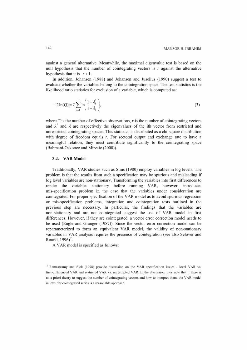
against a general alternative. Meanwhile, the maximal eigenvalue test is based on the null hypothesis that the number of cointegrating vectors is r against the alternative hypothesis that it is 1+r .
In addition, Johansen (1988) and Johansen and Juselius (1990) suggest a test to evaluate whether the variables belong to the cointegration space. The test statistics is the likelihood ratio statistics for exclusion of a variable, which is computed as:
∑=
⎟⎟⎠
⎞⎜⎜⎝
⎛
−−
=−r
i i
iTQ1
*
11ln)ln(2
λλ , (3)
where T is the number of effective observations, r is the number of cointegrating vectors, and λ* and λ are respectively the eigenvalues of the ith vector from restricted and unrestricted cointegrating spaces. This statistics is distributed as a chi-square distribution with degree of freedom equals r. For sectoral output and exchange rate to have a meaningful relation, they must contribute significantly to the cointegrating space (Bahmani-Oskooee and Mirzaie (2000)).
3.2. VAR Model Traditionally, VAR studies such as Sims (1980) employ variables in log levels. The
problem is that the results from such a specification may be spurious and misleading if log level variables are non-stationary. Transforming the variables into first differences to render the variables stationary before running VAR, however, introduces mis-specification problem in the case that the variables under consideration are cointegrated. For proper specification of the VAR model as to avoid spurious regression or mis-specification problems, integration and cointegration tests outlined in the previous step are necessary. In particular, the findings that the variables are non-stationary and are not cointegrated suggest the use of VAR model in first differences. However, if they are cointegrated, a vector error correction model needs to be used (Engle and Granger (1987)). Since the vector error correction model can be reparameterized to form an equivalent VAR model, the validity of non-stationary variables in VAR analysis requires the presence of cointegration (see also Selover and Round, 1996)2.
A VAR model is specified as follows:
2 Ramaswamy and Slok (1998) provide discussion on the VAR specification issues - level VAR vs. first-differenced VAR and restricted VAR vs. unrestricted VAR. In the discussion, they note that if there is no a priori theory to suggest the number of cointegrating vectors and how to interpret them, the VAR model in level for cointegrated series is a reasonable approach.
SECTORAL EFFECTS OF RINGGIT DEPRECIATION SHOCKS 143
t
p
kktkt eXAAX ++= ∑
=−
10 , (4)
where is an vector of variables, is an tX 1×n 0A 1×n vector of constant terms,
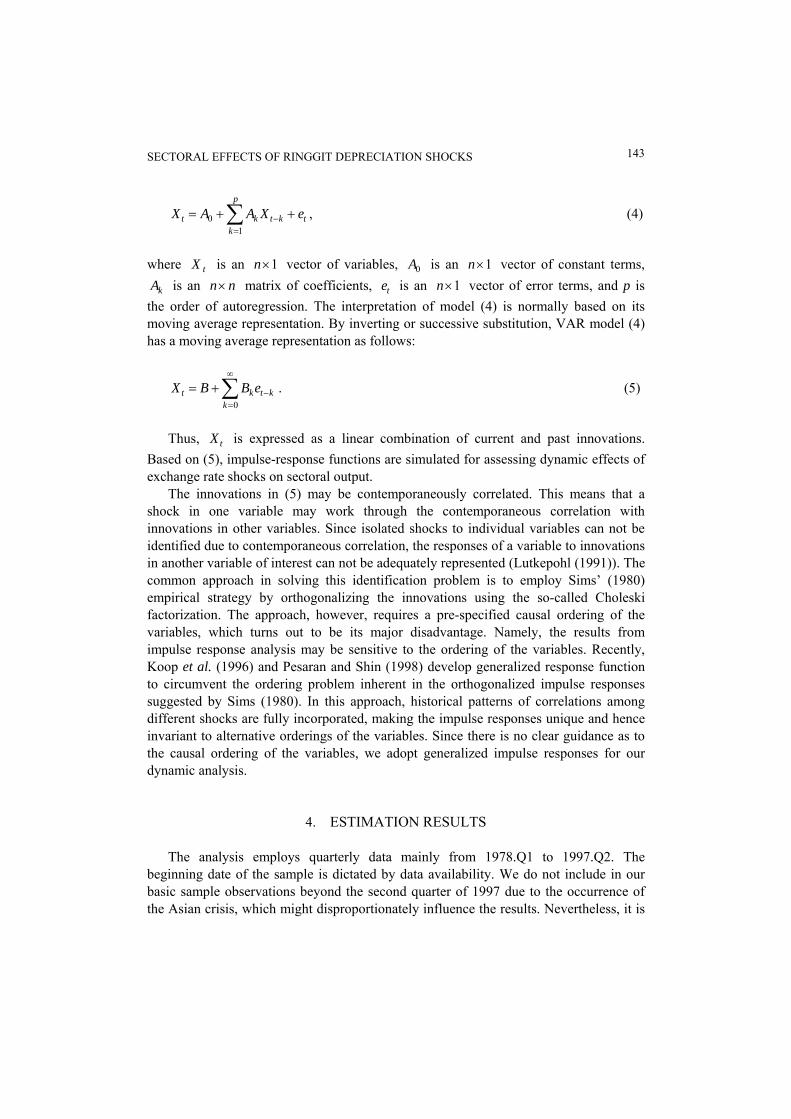
is an matrix of coefficients, is an kA nn× te 1×n vector of error terms, and p is the order of autoregression. The interpretation of model (4) is normally based on its moving average representation. By inverting or successive substitution, VAR model (4) has a moving average representation as follows:
∑∞
=−+=
0kktkt eBBX . (5)
Thus, is expressed as a linear combination of current and past innovations.
Based on (5), impulse-response functions are simulated for assessing dynamic effects of exchange rate shocks on sectoral output.
tX
The innovations in (5) may be contemporaneously correlated. This means that a shock in one variable may work through the contemporaneous correlation with innovations in other variables. Since isolated shocks to individual variables can not be identified due to contemporaneous correlation, the responses of a variable to innovations in another variable of interest can not be adequately represented (Lutkepohl (1991)). The common approach in solving this identification problem is to employ Sims’ (1980) empirical strategy by orthogonalizing the innovations using the so-called Choleski factorization. The approach, however, requires a pre-specified causal ordering of the variables, which turns out to be its major disadvantage. Namely, the results from impulse response analysis may be sensitive to the ordering of the variables. Recently, Koop et al. (1996) and Pesaran and Shin (1998) develop generalized response function to circumvent the ordering problem inherent in the orthogonalized impulse responses suggested by Sims (1980). In this approach, historical patterns of correlations among different shocks are fully incorporated, making the impulse responses unique and hence invariant to alternative orderings of the variables. Since there is no clear guidance as to the causal ordering of the variables, we adopt generalized impulse responses for our dynamic analysis.
4. ESTIMATION RESULTS
The analysis employs quarterly data mainly from 1978.Q1 to 1997.Q2. The beginning date of the sample is dictated by data availability. We do not include in our basic sample observations beyond the second quarter of 1997 due to the occurrence of the Asian crisis, which might disproportionately influence the results. Nevertheless, it is
MANSOR H. IBRAHIM 144
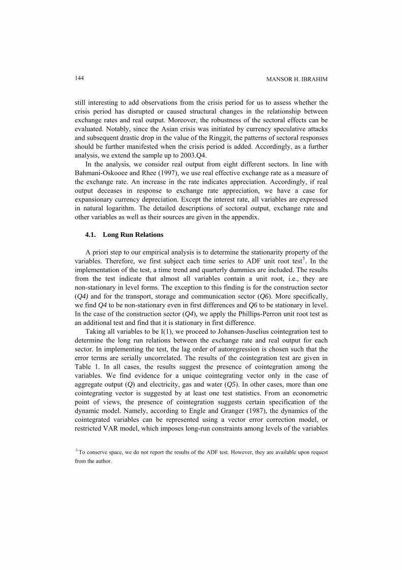
still interesting to add observations from the crisis period for us to assess whether the crisis period has disrupted or caused structural changes in the relationship between exchange rates and real output. Moreover, the robustness of the sectoral effects can be evaluated. Notably, since the Asian crisis was initiated by currency speculative attacks and subsequent drastic drop in the value of the Ringgit, the patterns of sectoral responses should be further manifested when the crisis period is added. Accordingly, as a further analysis, we extend the sample up to 2003.Q4.
In the analysis, we consider real output from eight different sectors. In line with Bahmani-Oskooee and Rhee (1997), we use real effective exchange rate as a measure of the exchange rate. An increase in the rate indicates appreciation. Accordingly, if real output deceases in response to exchange rate appreciation, we have a case for expansionary currency depreciation. Except the interest rate, all variables are expressed in natural logarithm. The detailed descriptions of sectoral output, exchange rate and other variables as well as their sources are given in the appendix.
4.1. Long Run Relations A priori step to our empirical analysis is to determine the stationarity property of the
variables. Therefore, we first subject each time series to ADF unit root test3. In the implementation of the test, a time trend and quarterly dummies are included. The results from the test indicate that almost all variables contain a unit root, i.e., they are non-stationary in level forms. The exception to this finding is for the construction sector (Q4) and for the transport, storage and communication sector (Q6). More specifically, we find Q4 to be non-stationary even in first differences and Q6 to be stationary in level. In the case of the construction sector (Q4), we apply the Phillips-Perron unit root test as an additional test and find that it is stationary in first difference.
Taking all variables to be I(1), we proceed to Johansen-Juselius cointegration test to determine the long run relations between the exchange rate and real output for each sector. In implementing the test, the lag order of autoregression is chosen such that the error terms are serially uncorrelated. The results of the cointegration test are given in Table 1. In all cases, the results suggest the presence of cointegration among the variables. We find evidence for a unique cointegrating vector only in the case of aggregate output (Q) and electricity, gas and water (Q5). In other cases, more than one cointegrating vector is suggested by at least one test statistics. From an econometric point of views, the presence of cointegration suggests certain specification of the dynamic model. Namely, according to Engle and Granger (1987), the dynamics of the cointegrated variables can be represented using a vector error correction model, or restricted VAR model, which imposes long-run constraints among levels of the variables
3 To conserve space, we do not report the results of the ADF test. However, they are available upon request from the author.

SECTORAL EFFECTS OF RINGGIT DEPRECIATION SHOCKS 145
as implied by their cointegration. Further, they note that these long-run constraints are also satisfied asymptotically in level VAR, or unrestricted VAR model. In other words, both approaches are appropriate for modeling dynamic interactions among time series. In this paper, we employ an unrestricted VAR model for our dynamic analysis.
Table 1. Cointegration Tests Test Null Hypothesis System Statistics r =0 r ≤ 1 r ≤ 2 r ≤ 3 r ≤ 4 r ≤ 5 Q Trace
Max 88.86*
42.79*46.07 25.35
20.72 13.64
7.07 6.69
0.38 0.38
- -
Q1 Trace Max
130.06*
43.11**86.95*
37.31**49.64**
20.60 29.03 18.29
10.74 8.84
1.90 1.90
Q2 Trace Max
127.00*
49.40*77.60*
36.28**41.32 20.22
21.10 13.50
7.60 6.94
0.66 0.66
Q3 Trace Max
127.45*
42.94**84.51*
37.08**47.44**
26.49 20.95 14.30
6.65 6.01
0.64 0.64
Q4 Trace Max
122.77*
42.31**80.46*
31.11 49.35**
26.20 23.15 13.66
9.49 6.75
2.74 2.74
Q5 Trace Max
119.34*
52.12*67.22 28.49
38.73 18.08
20.66 10.68
9.98 9.16
0.81 0.81
Q6 Trace Max
125.09*
45.43*79.66*
35.62**44.04 21.85
22.19 14.74
7.45 7.20
0.25 0.25
Q7 Trace Max
129.61*
58.09*71.52**
32.82 38.70 23.85
14.85 8.40
6.45 6.38
0.07 0.07
Q8 Trace Max
146.60*
57.36*89.24*
42.64*46.59 23.51
23.08 14.99
8.09 6.99
1.10 1.10
Notes: GDP = aggregate output, Q1 = Agriculture, Forestry and Fishing, Q2 = Mining and Quarrying, Q3 = Manufacturing, Q4 = Construction, Q5 = Electricity, Gas and Water, Q6 = Transport, Storage and Communication, Q7 = Wholesales and Retail Trade, Q8 = Finance, Insurance, Real estates and Business Services. *, ** denote significance level at 1% and 5% respectively.
The presence of cointegration also suggests that there is a long run relationship
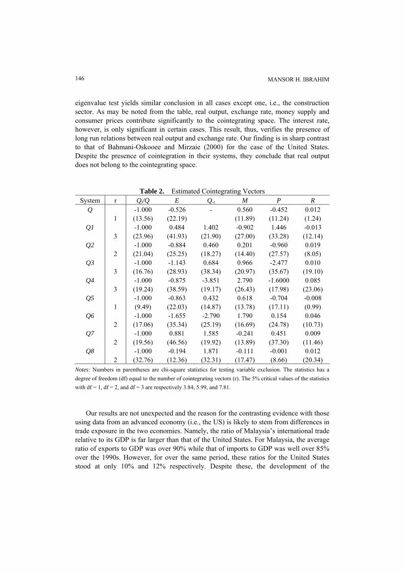
among the variables in the system. However, for our long run analysis to be meaningful, both the exchange rate and real output must contribute significantly to the cointegration space. Table 2 reports a cointegrating vector that corresponds to the largest eigenvalue for each system together with chi-square test statistics for the exclusion of the variables. In the cases that the trace test and maximal eigenvalue test suggest different number of cointegrating vectors, we report only the likelihood ratio test based on the number of cointegrating vector as suggested by the trace test. However, in these cases, it is pleased to note that the likelihood ratio statistics computed based on results from the maximal
MANSOR H. IBRAHIM 146
eigenvalue test yields similar conclusion in all cases except one, i.e., the construction sector. As may be noted from the table, real output, exchange rate, money supply and consumer prices contribute significantly to the cointegrating space. The interest rate, however, is only significant in certain cases. This result, thus, verifies the presence of long run relations between real output and exchange rate. Our finding is in sharp contrast to that of Bahmani-Oskooee and Mirzaie (2000) for the case of the United States. Despite the presence of cointegration in their systems, they conclude that real output does not belong to the cointegrating space.
Table 2. Estimated Cointegrating Vectors System r Qi/Q E Q-i M P R
Q 1
-1.000 (13.56)
-0.526 (22.19)
- 0.560 (11.89)
-0.452 (11.24)
0.012 (1.24)
Q1 3
-1.000 (23.96)
0.484 (41.93)
1.402 (21.90)
-0.902 (27.00)
1.446 (33.28)
-0.013 (12.14)
Q2 2
-1.000 (21.04)
-0.884 (25.25)
0.460 (18.27)
0.201 (14.40)
-0.960 (27.57)
0.019 (8.05)
Q3 3
-1.000 (16.76)
-1.143 (28.93)
0.684 (38.34)
0.966 (20.97)
-2.477 (35.67)
0.010 (19.10)
Q4 3
-1.000 (19.24)
-0.875 (38.59)
-3.851 (19.17)
2.790 (26.43)
-1.6000 (17.98)
0.085 (23.06)
Q5 1
-1.000 (9.49)
-0.863 (22.03)
0.432 (14.87)
0.618 (13.78)
-0.704 (17.11)
-0.008 (0.99)
Q6 2
-1.000 (17.06)
-1.655 (35.34)
-2.790 (25.19)
1.790 (16.69)
0.154 (24.78)
0.046 (10.73)
Q7 2
-1.000 (19.56)
0.881 (46.56)
1.585 (19.92)
-0.241 (13.89)
0.451 (37.30)
0.009 (11.46)
Q8 2
-1.000 (32.76)
-0.194 (12.36)
1.871 (32.31)
-0.111 (17.47)
-0.001 (8.66)
0.012 (20.34)
Notes: Numbers in parentheses are chi-square statistics for testing variable exclusion. The statistics has a degree of freedom (df) equal to the number of cointegrating vectors (r). The 5% critical values of the statistics with df = 1, df = 2, and df = 3 are respectively 3.84, 5.99, and 7.81.
Our results are not unexpected and the reason for the contrasting evidence with those
using data from an advanced economy (i.e., the US) is likely to stem from differences in trade exposure in the two economies. Namely, the ratio of Malaysia’s international trade relative to its GDP is far larger than that of the United States. For Malaysia, the average ratio of exports to GDP was over 90% while that of imports to GDP was well over 85% over the 1990s. However, for over the same period, these ratios for the United States stood at only 10% and 12% respectively. Despite these, the development of the
SECTORAL EFFECTS OF RINGGIT DEPRECIATION SHOCKS 147
Malaysian financial markets far lags behind that of the United States. With the developed capital markets, firms in the United States are in better position to hedge against risks such as the exchange rate risk. The hedging opportunity of the Malaysian firms, however, is limited. Apart from these reasons, Andersen and Tarp (2003) note that developing economies are comparatively more volatile and less diversified. As a result, fluctuations in the exchange rate can have strong effects. We believe that these factors make the exchange rate to be an important factor in accounting for macroeconomic performance of the Malaysian economy while it is not for the United States.
It is clear from the table that, in the aggregate output system, exchange rate appreciation is associated with the reduction in real output. Meanwhile, as should be expected, the long run relation between money and aggregate output is positive while that between prices and output is negative. The interest rate, however, does not seem to belong to the equation. The long run relation, thus, is supportive of the conventional view that the exchange rate depreciation is expansionary for the case of Malaysia. This finding is consistent with that of Bahmani-Oskooee and Rhee (1997). Namely, they also find evidence for the expansionary effect of currency depreciation for the case of Korea. A possible common reason is that both economies, Malaysia and Korea, are highly export oriented.
Our analysis using sectoral output reveals several interesting results. In line with the result for aggregate output, currency depreciation is expansionary for most sectors. However, the estimated coefficient of the exchange rate seems to differ markedly across sectors. The reported negative coefficient of the exchange rate seems to be lowest for finance, insurance, real estates and business services (Q8) and highest for transport, storage and communication (Q6). The equation for manufacturing sector (Q3) also seems to have high estimated long run coefficient of the exchange rate, suggesting its vulnerability to exchange rate changes in the long run. Among the eight sectors considered, only two sectors seem to be adversely affected by currency depreciation. These sectors are agriculture, forestry and fishing (Q1) and wholesales and retail trade (Q7). These results, thus, are indicative of differential effects of currency depreciation, the dynamics of which is discussed next.
For other variables, the results conform well to those of the aggregate output system with positive money supply coefficient and negative price coefficient in most cases. It is also worthwhile to note that other sectoral output (aggregate output less sectoral output under consideration) contributes significantly to their respective cointegrating equations. This suggests inter-linkages among the various sectors and, in many cases, there exist positive linkages between them.
4.2. Generalized Impulse Responses To trace the dynamic responses of sectoral output to and evaluate the differential
effects of exchange rate shocks, we simulate generalized impulse responses from estimated dynamic models. As we have noted, given the finding of cointegration, we
MANSOR H. IBRAHIM 148
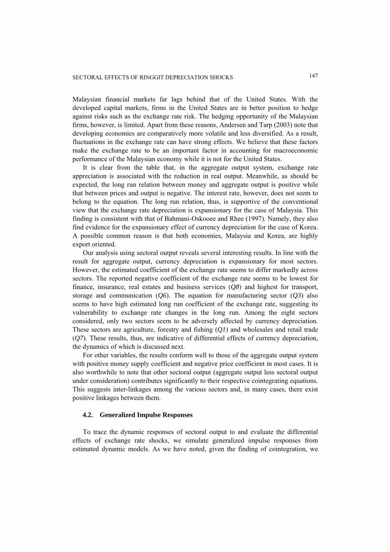
estimate VAR in level for all cases. Again, the order of the VAR is chosen such that the error terms are serially uncorrelated. The graphical plots of these responses are presented in Figure 1. For comparative purposes, we also plot the responses of aggregate output to the exchange rate shocks. In general, the results seem to conform to the long run results in that, in most cases, the exchange rate depreciation (appreciation) is expansionary (contractionary). Moreover, the generalized impulse responses further indicate distributional consequences of currency shocks.
-0.015
-0.01
-0.005
0
0.
0.01
005
1 2 3 4 5 6 7 8 9 10 11 12 13 14 15 16 17 18 19 20 21 22 23 24
Aggregate Output Q1 Q2
(a) Agriculture, Forestry and Fishing (Q1) and Mining and Quarrying (Q2)
-0.025
-0.02
-0.015
-0.01
-0.005
0
0.005
0.01
0.015
0.02
1 2 3 4 5 6 7 8 9 10 11 12 13 14 15 16 17 18 19 20 21 22 23 24
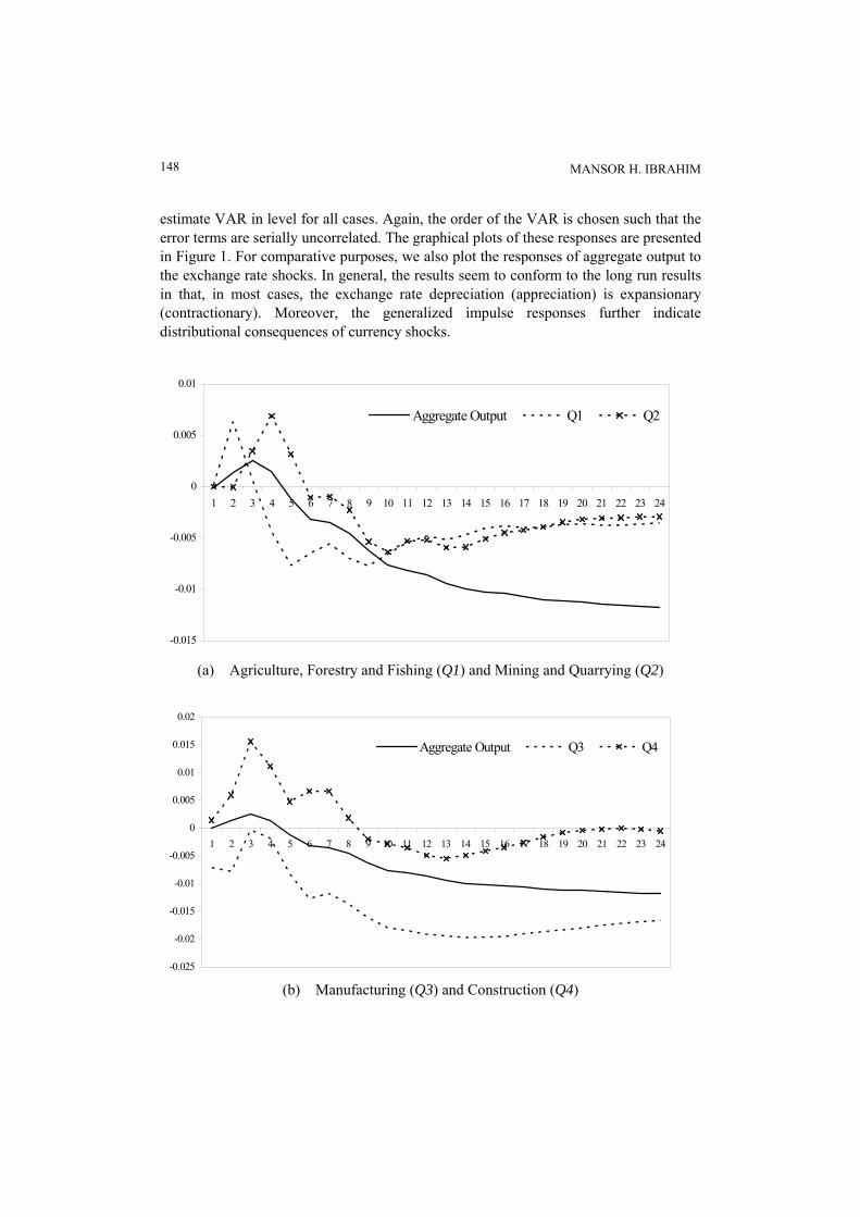
Aggregate Output Q3 Q4
(b) Manufacturing (Q3) and Construction (Q4)
SECTORAL EFFECTS OF RINGGIT DEPRECIATION SHOCKS 149
-0.0
-0.0
-0.0
-0.0
0.01
0.02
1 2 3 4 5 6 7 8 9 10 11 12 13 14 15 16 17 18 19 20 21 22 23 24
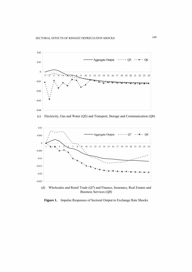
Aggregate Output Q5 Q6
0
1
2
3
4
(c) Electricity, Gas and Water (Q5) and Transport, Storage and Communication (Q6)
-0.0
-0.
-0.0
-0.
-0.0
0.0
0.
1 2 3 4 5 6 7 8 9 10 11 12 13 14 15 16 17 18 19 20 21 22 23 24
01
25
02
15
01
05
0
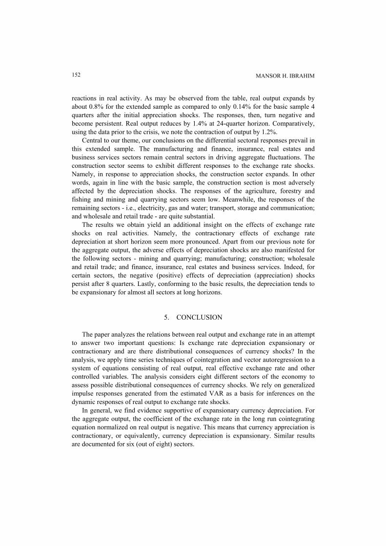
05 Aggregate Output Q7 Q8 (d) Wholesales and Retail Trade (Q7) and Finance, Insurance, Real Estates and
Business Services (Q8)
Figure 1. Impulse Responses of Sectoral Output to Exchange Rate Shocks

MANSOR H. IBRAHIM 150
From the figure, we may note that the temporal reaction of aggregate output seems to resemble the J-curve phenomenon documented in the international trade literature. Specifically, in response to exchange rate appreciation shocks, real output first increases and then, after about 4 quarters, decreases and the responses remain negative throughout the 24-quarter horizon. To put in a different way, following exchange rate depreciation shocks, real output reacts negatively first and then positively. Glancing through Figure 1(a) to 1(d), we may note differential responses of various sectors to the currency effects. Namely, the responses of some sectors seem to be more amplified.
The temporal pattern of sectoral output responses to exchange rate shocks seem to be similar to that of the aggregate output for agriculture, forestry and fishing and mining and quarrying sectors (Figure 1(a)). Namely, their responses to exchange rate appreciation are first positive and then turn negative. It should be noted that the negative effect appears transitory and not significant. The responses of the construction seem to follow a similar pattern (Figure 1(b)). However, it seems to be affected most by currency shocks at short horizons, suggesting the strong adverse effect of the depreciation shocks. Despite the fact that we exclude the Asian crisis period, this result conforms well to what we observed during the crisis, i.e., the construction sector has the biggest contraction following currency depreciation shocks.
The negative effect of currency appreciation shocks seems immediate and more amplified for the manufacturing sector (Figure 1(b)). This result should be expected as the manufacturing sector has the greatest trade (i.e., exports) exposure. The immediate negative responses are also observed for the electricity, gas and water and transport, storage and communication sectors (Figure 1(c)), as well. However, for these sectors, their responses to the exchange rate shocks seem to track the aggregate responses very well. Lastly, while the temporal responses of the wholesale and trade sector are similar the aggregate responses, those of finance, insurance, real estates and business services seem amplified as in the case of the manufacturing sector.
From the foregoing discussion, we may say that fluctuations in aggregate output is driven particularly by the manufacturing sector and the finance, insurance, real estates and business services sector. The manufacturing sector being the driving force of the Malaysian economy is well noted, while continuous liberalization and integration of the financial markets have considerably propel the progress of the finance, insurance, real estates and business services sector. Perhaps, increasing exposure of these sectors to international environments make them to be very responsive to the exchange rate shocks. Moreover, based on our documented dynamics, we may also conclude that, at short horizons, currency depreciation can be contractionary particularly for the construction sector. However, at longer horizons, it tends to be expansionary.
4.3. Further Analysis It needs mentioning that the foregoing results are not inconsistent with the observed
dynamics of the Asian crisis, specifically, on how real economic activities react to

SECTORAL EFFECTS OF RINGGIT DEPRECIATION SHOCKS 151
currency shocks. During the crisis, the initial responses to depreciation shocks seem to be negative for many sectors. Then, they recovered quickly forming the well-known V-shaped recovery. We believe that, since the Asian crisis was initiated by currency speculative attacks and subsequent drastic drop in the value of the Ringgit, the patterns of sectoral responses should be further manifested when the crisis period is added. Moreover, the Asian crisis period may have disrupted or caused structural changes in the relationship between exchange rates and real output. To ascertain these, we further analyze the exchange rate - real output relations by extending the sample up to 2003.Q4.
Table 3. Impulse Response Functions - Basic and Extended Samples Basic Sample (1978.1-1997.2) Extended Sample (1978.1-2003.4)
Output 4 8 Max 4 8 Max GDP 0.0014 -0.0046 -0.0118 [24] 0.0080 -0.0043 -0.0140 [24] Q1 -0.0044 -0.0070 -0.0077 [9] -0.0001 -0.0024 -0.0054 [13] Q2 0.0069 -0.0023 -0.0064 [10] 0.0049 0.0012 -0.0028 [11] Q3 -0.0018 -0.0136 -0.0197 [14] 0.0086 -0.0136 -0.0260 [12] Q4 0.0112 0.0018 0.0067 [7] 0.0413 0.0283 0.0367 [6] Q5 -0.0028 -0.0006 -0.0114 [24] -0.0036 -0.0069 -0.0116 [24] Q6 -0.0168 -0.0088 -0.0168 [4] -0.0093 -0.0066 -0.0169 [16] Q7 0.0075 -0.0004 -0.0130 [15] 0.0117 0.0017 -0.0109 [24] Q8 -0.0050 -0.0113 -0.0191 [24] 0.0064 -0.0046 -0.0165 [16]
Notes: Numbers in squared brackets are quarters at which the responses of output to exchange rate shocks reach their peaks (minimum or maximum). If the quarter indicated is 24, it means that the responses are not reverting back to zero; i.e., they are persistence.
Since our results suggest that the variables under analysis remain cointegrated, we
focus on dynamic responses of various output measures to exchange rate shocks in this subsection. Rather than plotting their temporal responses, we summarize the results in Table 34. In specific, we present the responses of the output measures at 4-quarter and 8-quarter horizons as well as their peaked responses. The quarter at which the response reaches its peak is also indicated. Note that if it is quarter 24 then it means that the responses do not die down to zero but remain persistent. These responses are tabulated for both our basic sample discussed in the previous section and the extended sample for comparative purposes.
The aggregate output responses to exchange rate shocks conform well to those of the basic sample. However, the addition of the crisis period leads to more pronounced
4 Graphical plots of the impulse response functions for this extended sample are available upon request from the author.
MANSOR H. IBRAHIM 152
reactions in real activity. As may be observed from the table, real output expands by about 0.8% for the extended sample as compared to only 0.14% for the basic sample 4 quarters after the initial appreciation shocks. The responses, then, turn negative and become persistent. Real output reduces by 1.4% at 24-quarter horizon. Comparatively, using the data prior to the crisis, we note the contraction of output by 1.2%.
Central to our theme, our conclusions on the differential sectoral responses prevail in this extended sample. The manufacturing and finance, insurance, real estates and business services sectors remain central sectors in driving aggregate fluctuations. The construction sector seems to exhibit different responses to the exchange rate shocks. Namely, in response to appreciation shocks, the construction sector expands. In other words, again in line with the basic sample, the construction section is most adversely affected by the depreciation shocks. The responses of the agriculture, forestry and fishing and mining and quarrying sectors seem low. Meanwhile, the responses of the remaining sectors - i.e., electricity, gas and water; transport, storage and communication; and wholesale and retail trade - are quite substantial.
The results we obtain yield an additional insight on the effects of exchange rate shocks on real activities. Namely, the contractionary effects of exchange rate depreciation at short horizon seem more pronounced. Apart from our previous note for the aggregate output, the adverse effects of depreciation shocks are also manifested for the following sectors - mining and quarrying; manufacturing; construction; wholesale and retail trade; and finance, insurance, real estates and business services. Indeed, for certain sectors, the negative (positive) effects of depreciation (appreciation) shocks persist after 8 quarters. Lastly, conforming to the basic results, the depreciation tends to be expansionary for almost all sectors at long horizons.
5. CONCLUSION The paper analyzes the relations between real output and exchange rate in an attempt
to answer two important questions: Is exchange rate depreciation expansionary or contractionary and are there distributional consequences of currency shocks? In the analysis, we apply time series techniques of cointegration and vector autoregression to a system of equations consisting of real output, real effective exchange rate and other controlled variables. The analysis considers eight different sectors of the economy to assess possible distributional consequences of currency shocks. We rely on generalized impulse responses generated from the estimated VAR as a basis for inferences on the dynamic responses of real output to exchange rate shocks.
In general, we find evidence supportive of expansionary currency depreciation. For the aggregate output, the coefficient of the exchange rate in the long run cointegrating equation normalized on real output is negative. This means that currency appreciation is contractionary, or equivalently, currency depreciation is expansionary. Similar results are documented for six (out of eight) sectors.

SECTORAL EFFECTS OF RINGGIT DEPRECIATION SHOCKS 153
The generalized impulse responses further substantiate the case for expansionary depreciation especially at longer horizons. However, the impulse responses further highlight possible contractionary depreciation at short horizons. Namely, we note that aggregate output and sectoral output from four sectors - agriculture, forestry and fishing; mining and quarrying; construction; wholesales and retail trade - reacts positively (negatively) first to appreciation (depreciation) shocks during the first 3-8 month horizons. Among these sectors, the construction sector seems to be most affected. At longer horizons, output from the manufacturing sector and the finance, insurance, real estates and business services sector seem to drive aggregate output. Their responses to appreciation shocks seem to be more pronounced than that of the aggregate output. Adding observations from the crisis period does not materially affect our results. Indeed, the short run contractionary effects of the exchange rate shocks and long run expansionary effects become stronger in the extended sample. Taken all these results together, we tend to provide affirmative answer to the second question. Namely, currency shocks are likely to have distributional consequences.
From policy points of view, contradicting Bahmani-Oskooee and Mirzaie (2000) for the United States, Malaysia can devalue (deliberately attempt to depreciate its currency) to boost its economic activities. However, two important cautions need to be noted. First, some sectors of the economy may be adversely affected. And second, currency depreciation may have distributional consequences. Accordingly, an attempt to achieve one objective (increasing real output) may come at the expense of unequal income distribution. In short, this aspect of currency depreciation needs to be taken into consideration when attempting to devalue the currency.
We believe that our results are equally applicable to other emerging markets of East Asia such as South Korea. The emerging economies of East Asia have adopted a similar path of development through export-led growth strategies and industrialization process. Accordingly, they become more open and highly susceptible to exchange rate fluctuations. We seem to believe that the concurrent contraction in their real activities during the Asian crisis and quick recovery perhaps reflects their similar responses to the exchange rate adjustments and shocks. To be certain, however, the extension of our analysis to other Asian countries is needed.
MANSOR H. IBRAHIM 154
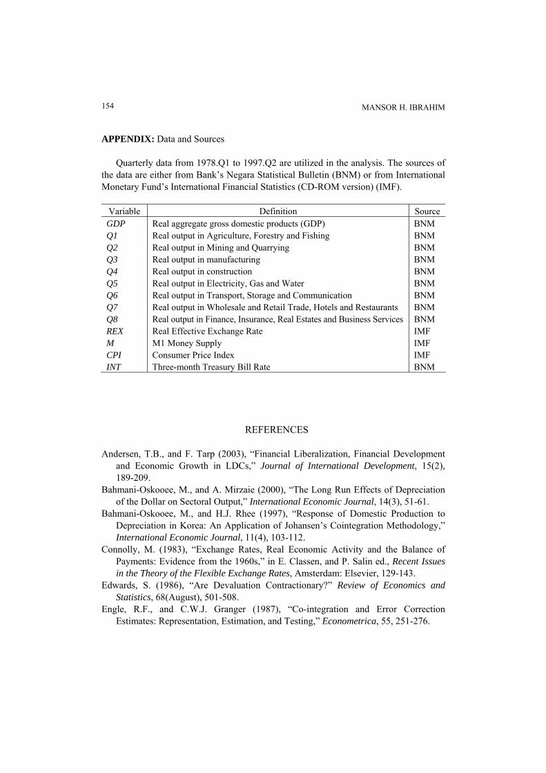
APPENDIX: Data and Sources
Quarterly data from 1978.Q1 to 1997.Q2 are utilized in the analysis. The sources of the data are either from Bank’s Negara Statistical Bulletin (BNM) or from International Monetary Fund’s International Financial Statistics (CD-ROM version) (IMF).
Variable Definition Source GDP Real aggregate gross domestic products (GDP) BNM Q1 Real output in Agriculture, Forestry and Fishing BNM Q2 Real output in Mining and Quarrying BNM Q3 Real output in manufacturing BNM Q4 Real output in construction BNM Q5 Real output in Electricity, Gas and Water BNM Q6 Real output in Transport, Storage and Communication BNM Q7 Real output in Wholesale and Retail Trade, Hotels and Restaurants BNM Q8 Real output in Finance, Insurance, Real Estates and Business Services BNM REX Real Effective Exchange Rate IMF M M1 Money Supply IMF CPI Consumer Price Index IMF INT Three-month Treasury Bill Rate BNM
REFERENCES
Andersen, T.B., and F. Tarp (2003), “Financial Liberalization, Financial Development and Economic Growth in LDCs,” Journal of International Development, 15(2), 189-209.
Bahmani-Oskooee, M., and A. Mirzaie (2000), “The Long Run Effects of Depreciation of the Dollar on Sectoral Output,” International Economic Journal, 14(3), 51-61.
Bahmani-Oskooee, M., and H.J. Rhee (1997), “Response of Domestic Production to Depreciation in Korea: An Application of Johansen’s Cointegration Methodology,” International Economic Journal, 11(4), 103-112.
Connolly, M. (1983), “Exchange Rates, Real Economic Activity and the Balance of Payments: Evidence from the 1960s,” in E. Classen, and P. Salin ed., Recent Issues in the Theory of the Flexible Exchange Rates, Amsterdam: Elsevier, 129-143.
Edwards, S. (1986), “Are Devaluation Contractionary?” Review of Economics and Statistics, 68(August), 501-508.
Engle, R.F., and C.W.J. Granger (1987), “Co-integration and Error Correction Estimates: Representation, Estimation, and Testing,” Econometrica, 55, 251-276.
SECTORAL EFFECTS OF RINGGIT DEPRECIATION SHOCKS 155
Gylfason, T., and M. Radetzki (1991), “Does Devaluation Make Sense in the Least Developed Countries?” Economic Development and Cultural Change, October, 1-25.
Gylfason, T., and M. Schmid (1983), “Does Devaluation Cause Stagflation?” Canadian Journal of Economics, 16(November), 641-654.
Gylfason, T., and O. Risager (1984), “Does Devaluation Improve the Current Account,” European Economic Review, 25(June), 37-64.
Johansen, J. (1988), “Statistical Analysis of Cointegrating Vectors,” Journal of Economic Dynamics and Control, 12, 231-54.
Johansen, J., and K. Juselius (1990), “Maximum Likelihood estimation and Inferences on Cointegration - With Application to the Demand for Money,” Oxford Bulletin of Economics and Statistics, 52, 169-210.
Kandil, M., and A. Mirzaie (2002), “Exchange Rate Fluctuations and Disaggregated Economic Activity in the US: Theory and Evidence,” Journal of International Money and Finance, 21, 1-31.
Koop, G., Pesran, M.H., and S.M. Potter (1996), “Impulse Response Analysis in Nonlinear Multivariate Models,” Journal of Econometrics, 74, 119-147.
Krugman, P., and L. Taylor (1978), “Contractionary Effect of Devaluation,” Journal of International Economics, 8(August), 445-56.
Lutkepohl, H. (1991), Introduction to Multiple Time Series Analysis, Berlin: Springer-Verlag.
Nelson, C.R., and C.I. Plosser (1982), “Trends and Random Walks in Macroeconomic Time Series: Some Evidence and Implications,” Journal of Monetary Economics, 10, 139-162.
Pesaran, M.H., and Y. Shin (1998), “Generalized Impulse Response Analysis in Linear Multivariate Models,” Economics Letters, 85, 17-29.
Ramaswamy, R., and T. Slok (1998), “The Real Effects of Monetary Policy in The European Union: What are the Differences?” IMF Staff Papers, 45(2), 374-396.
Selover, D.D., and D.K. Round (1996), “Business Cycle Transmission and Interdependence between Japan and Aystralia,” Journal of Asian Economics, 7(4), 569-602.
Sims, C.A. (1980), “Macroeconomics and Reality,” Econometrica, 48, 1-48. Solimano, A. (1986), “Contractionary Devaluation in the Southern Cone: The Case of
Chile,” Journal of Development Economics, September, 135-151. Tatom, J.A. (1987), “Will a Weaker Dollar Mean a Stronger Economy?” Journal of
International Money and Finance, December, 433-447. _____ (1988), “The Link Between the Value of the Dollar, U.S. Trade and
Manufacturing Output: Some Recent Evidence,” Federal Reserve Bank of St. Louis Review, November/December, 24-37.
Upadhyaya, K.P. (1999), “Currency Devaluation, Aggregate Output, and the Long Run: An Empirical Study,” Economics Letters, 64, 197-202.

MANSOR H. IBRAHIM 156
Upadhyaya, K.P., and M.P. Upadhyay (1999), “Output Effects of Devaluation: Evidence From Asia,” Journal of Development Studies, 35(6), 89-103.
Mailing Address: Department of Economics, IIUM, KM16, Jalan Gombak 53100, Kuala Lumpur, Malaysia. E-mail: [email protected].
Manuscript received March 2003; final revision received August, 2007.