pdf book file - ucsf macromolecular structure group
TRANSCRIPT

KaleidaGraph ®
Version 3.6
Note: For optimal viewing of this file, choose File > Preferences > General and select the Display Page to Edge option.


Introduction
the s tha
tep-by
gging. Itons, anputer.
lots, and
ncepts
g an
and
the
data
simila
rids,
r bar
Welcome to KaleidaGraph®. You have purchased a thoughtfully designed graphing tool which providesmost powerful visual displays of quantitative information available in either the Windows or Macintoshenvironment. Through our documentation, you will learn how to develop accurate journal quality graphtmathematically transform even the most complex data into elegant but functional graphical displays.
About this ManualThis manual contains detailed cross-platform information about the KaleidaGraph application. It provides s-step instructions for the Windows and Macintosh platforms. Wherever there is a difference between the two platforms, it is noted in the text.
The manual assumes that you are familiar with basic operations, such as clicking, double-clicking, and dratalso assumes familiarity with the components of the user interface, such as menus, windows, dialogs, butdcheck boxes. If you are not familiar with these terms, review the documentation that came with your com
Organization of the ManualThis manual contains examples and procedures for common tasks, such as entering data, creating papplying curve fits. The following is a brief overview of the chapters and appendixes in the manual:
• Chapter 1, “Getting Started,” discusses system requirements, installation, and several basic co,including opening files, getting help, and quitting the program.
• Chapter 2, “Guided Tour of KaleidaGraph,” provides a tutorial for generating a data set, creatindediting Scatter and Column plots, and placing the plots in the layout window.
• Chapter 3, “Working with Data Windows,” discusses how to navigate, make selections, add delete rows and columns, and format columns in the data window.
• Chapter 4, “Working with Data,” discusses how to enter, import, edit, sort, and export data indata window.
• Chapter 5, “Analyzing Data,” discusses how to view column statistics, bin data, and analyze using a number of parametric and nonparametric statistical tests
• Chapter 6, “Working with Formula Entry,” discusses how to use the Formula Entry window toperform calculations in the active data window.
• Chapter 7, “Creating Plots,” discusses the different plot types, creating a plot, and generating rplots.
• Chapter 8, “Working with Plots,” discusses how to modify the plot, including the axes, ticks, gmarkers, and plot color.
• Chapter 9, “Working with Plot Tools and Objects,” discusses the plot tools available in KaleidaGraph, in addition to creating and editing text labels and shapes.
• Chapter 10, “Working with Curve Fits and Error Bars,” discusses how to add curve fits and errosto a plot.
3

KaleidaGraph
a plo
lace
torial placing Entry,
mands
greate
e firs
clude
• Chapter 11, “Importing and Exporting Graphics,” discusses how to import graphic objects into tand export the plots to a printer, file, or another program.
• Chapter 12, “Working with the Layout Window,” discusses how to use the layout window to pmultiple plots on a single page.
• The Appendixes contain information on the program commands, settings files, and toolbox shortcuts, as well as general reference information.
Learning KaleidaGraphIf you are new to KaleidaGraph, it is recommended that you take the guided tour in Chapter 2. This tuguides you through the process of generating a data set, creating and editing two different plots, andthe plots onto a single page. Other topics in the tutorial include modifying the legend, using Formula applying a General curve fit, and modifying data in a saved plot.
Once you start using KaleidaGraph, you can refer to the manual and the online help for step-by-step instructions to complete specific tasks. The online help also includes detailed information on the comand dialogs available in the program.
ConventionsThis manual uses the following conventions:
• Instructions for choosing commands are displayed in bold type. Levels are separated with a rthan symbol (>). For example: Choose Gallery > Linear > Line.
• Dialog buttons and options are displayed in bold type. For example: Click OK .
• Keys that you should press appear in bold type. If joined with a plus sign (+), press and hold thtkey while you press the remaining keys. For example: Press Ctrl +Period.
Contacting Synergy SoftwareTo receive technical support and upgrade information, either fill out and send in the registration card indwith the software or access our web site and register online.
If you have any questions concerning KaleidaGraph, please contact us at:
Synergy Software2457 Perkiomen AvenueReading, PA 19606-2049 USA
Phone: (1) 610-779-0522Fax: (1) 610-370-0548
Internet addresses:Sales/Upgrades: [email protected] support: [email protected]
Web sites: www.kaleidagraph.comwww.synergy.com
4
Introduction
Please feel free to check our web site periodically for:
• Product descriptions
• Technical notes
• Frequently asked questions
• New release information
• Downloadable upgrade patches
• And other topics of interest
5

KaleidaGraph
6

Getting Started
Chapter 1
aGraph
This chapter lists the hardware and operating system requirements and explains how to install Kaleidonto your computer. It also covers some basic concepts, including:• Starting KaleidaGraph.
• Introducing the data and plot windows.
• Opening saved files.
• Opening KaleidaGraph files on another platform.
• Getting help.
• Setting preferences.
• Quitting the program.
1.1 System Requirements
Windows Version Macintosh Version
• A Pentium PC or faster computer equipped with a CD-ROM drive.
• Windows 98 or later (including Windows 2000, NT, ME, and XP).
• 32 MB of RAM. Additional RAM isrecommended and increases KaleidaGraph’s performance.
• 10-15 MB free hard disk space.
• A Power PC running System 8.6 or later. CarbonLib v1.6 will be installed if it is not present.
• OS X users should have OS 10.1.3 or later.
• 15 MB of free RAM is recommended.
• 15-20 MB free hard disk space.
1.1 System Requirements 7

KaleidaGraph
1.2 Installing KaleidaGraphThis section describes how to install the KaleidaGraph software on both the Windows and Macintosh platforms. A section containing uninstall instructions is also included.
1.2.1 Installing the Windows VersionThe installer creates a new folder on your hard disk containing the KaleidaGraph software. If you are upgrading from an earlier version, your existing KaleidaGraph files are not affected.
To install KaleidaGraph on your hard disk:
1. Quit any other programs that are currently running.
2. Insert the KaleidaGraph CD-ROM.
3. Run KG36Setup to install the software.
4. Proceed through the Welcome screen, ReadMe information, and license agreement.
5. Specify where to install the KaleidaGraph program and its related files. To specify a different directory, click Browse. When you are finished, click Next.
6. Choose the type of installation you want to perform and click Next to install the software. The choices are:
• Typical - installs all of the KaleidaGraph files.
• Compact - installs only the files needed to run KaleidaGraph.
• Custom - allows you to select which components to install.
7. If you have KaleidaGraph v3.5x already installed, you will be asked if you would like to have it uninstalled for you. If you choose to leave KaleidaGraph v3.5x on your computer, you can always uninstall it at a later time. It is valid to have multiple versions on the same computer.
8. The installer will also give you the opportunity to submit your registration information. By registering the software, you will receive free technical support and upgrade information.
9. Once all of the program files have been installed, a message is displayed to let you know the installation of KaleidaGraph is complete.
8 1.2 Installing KaleidaGraph

Getting Started
ay the
folde
an
ipped
tatu
u wil
tyle,
rences e
1.2.2 Installing the Macintosh VersionThe installer creates a new folder on your hard disk containing the KaleidaGraph software. If you areupgrading from an earlier version, your existing KaleidaGraph files are not affected.
To install KaleidaGraph on your hard disk:
1. Insert the KaleidaGraph CD-ROM.
2. Double-click the KaleidaGraph 3.6 Installer icon.
3. Proceed through the Welcome screen, license agreement, and ReadMe information to displKaleidaGraph Installer dialog.
4. Choose the installation method (easy or custom) and specify where to place the KaleidaGraphr
The Easy Install option automatically installs the following items:
• The KaleidaGraph application.
• An Examples folder containing example plots, data files, and curve fits.
• The QuickHelp application (if it is not already installed), along with the KaleidaGraph HelpdNew Features documents.
• A Manuals folder containing PDF versions of the KaleidaGraph documentation.
• For OS 9 and earlier, CarbonLib v1.6 is also installed. If this file is already present, it is sk
To control which files get installed, choose Custom Install from the pop-up menu.
5. Click Install . A KaleidaGraph folder is created on your hard disk and the files are installed. A Ssdialog is displayed to keep you informed as the installation progresses.
6. The installer will display a window so that you can submit your registration information. The registration form can be submitted by email, postal mail, or fax. By registering the software, yolreceive free technical support and upgrade information.
7. Once all of the program files have been installed, a message is displayed to let you know theinstallation of KaleidaGraph is complete.
Note: If you are updating from an earlier version, the default location for storing the settings files (KG SKG Macros, KG Layout, and KG Script) has changed. The settings files are now stored in the KaleidaGraph Preferences folder. The KaleidaGraph Preferences folder is located in the Prefefolder (in the users Library folder under OS X or in the System Folder for OS 9 and earlier). Thinstaller automatically moves a copy of the settings files into the new location.
1.2 Installing KaleidaGraph 9
KaleidaGraph
ay the
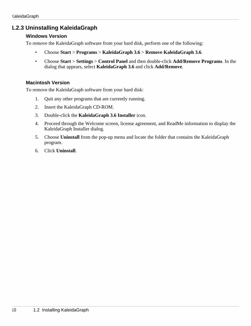
1.2.3 Uninstalling KaleidaGraphWindows VersionTo remove the KaleidaGraph software from your hard disk, perform one of the following:
• Choose Start > Programs > KaleidaGraph 3.6 > Remove KaleidaGraph 3.6.
• Choose Start > Settings > Control Panel and then double-click Add/Remove Programs. In the dialog that appears, select KaleidaGraph 3.6 and click Add/Remove.
Macintosh VersionTo remove the KaleidaGraph software from your hard disk:
1. Quit any other programs that are currently running.
2. Insert the KaleidaGraph CD-ROM.
3. Double-click the KaleidaGraph 3.6 Installer icon.
4. Proceed through the Welcome screen, license agreement, and ReadMe information to displKaleidaGraph Installer dialog.
5. Choose Uninstall from the pop-up menu and locate the folder that contains the KaleidaGraphprogram.
6. Click Uninstall.
10 1.2 Installing KaleidaGraph

Getting Started
ng files, also
m, the
sed anged
xt ormul
1.3 KaleidaGraph BasicsThis section introduces some of KaleidaGraph’s basic concepts, such as starting the program, openiand quitting the program. The various areas and terms associated with the data and plot windows areexplained.
1.3.1 Starting KaleidaGraphTo start KaleidaGraph, perform one of the following:
• Windows: Double-click the KGraph icon or choose Start > Programs > KaleidaGraph 3.6 > KGraph .
• Macintosh: Double-click the KaleidaGraph icon.
The first time the program is started, the dialog in Figure 1-1 is displayed to personalize your copy ofKaleidaGraph and enter your serial number and authorization code. If this is a new copy of the prograserial number is located on the back cover of the manual, or on your order confirmation if you purchaKaleidaGraph electronically. If this is an update from an earlier version, your serial number has not ch
Figure 1-1 Startup dialog
After you click OK , two windows are displayed; a data window and the Formula Entry window. The nesection contains an introduction to the data window. Refer to Chapter 6 for information on using the FaEntry window to analyze and manipulate data in the active data window.
1.3 KaleidaGraph Basics 11

KaleidaGraph
ng and m of
windo empty
r to a
ow.
1.3.2 Data Window OverviewThe data window, shown in Figure 1-2, contains a spreadsheet used to enter and store data for plottianalysis. It consists of a number of cells organized in columns. A data window can contain a maximu1000 columns and 1 million rows, subject to memory limitations.
Figure 1-2 Data window
1. Home ButtonClick this button to return the data window to its origin (row 0, column 0). This is useful for quicklyreturning to the start of the window when viewing a different section of the data window.
2. Cell Selection CursorThis cursor is used to make selections in the data window.
3. Posted NoteThe Posted Note is used to enter information about the data in the active data window. Each data whas its own Posted Note. When information is stored in the Posted Note, its icon changes from annote to one with data in it.
4. Title BarThe title bar displays the name of the file. You can move the data window by dragging the title banew location.
5. Update Plot ButtonClick this button to force an immediate update of the plot that is currently linked to this data wind
1
2
3
5
4
12 1.3 KaleidaGraph Basics
Getting Started
y of th
n
is
le
in the olum
ons
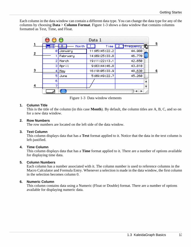
Each column in the data window can contain a different data type. You can change the data type for anecolumns by choosing Data > Column Format. Figure 1-3 shows a data window that contains columns formatted as Text, Time, and Float.
Figure 1-3 Data window elements
1. Column TitleThis is the title of the column (in this case Month ). By default, the column titles are A, B, C, and so ofor a new data window.
2. Row NumbersThe row numbers are located on the left side of the data window.
3. Text ColumnThis column displays data that has a Text format applied to it. Notice that the data in the text columnleft-justified.
4. Time ColumnThis column displays data that has a Time format applied to it. There are a number of options availabfor displaying time data.
5. Column NumbersEach column has a number associated with it. The column number is used to reference columnsMacro Calculator and Formula Entry. Whenever a selection is made in the data window, the first cnin the selection becomes column 0.
6. Numeric ColumnThis column contains data using a Numeric (Float or Double) format. There are a number of optiavailable for displaying numeric data.
1
2
3
4
5
6
1.3 KaleidaGraph Basics 13

KaleidaGraph
re 1-4
g the
e object
e plot,
1.3.3 Plot Window OverviewPlots are created by entering data into the data window and choosing a plot type from the Gallery menu. Afterselecting the data columns to be plotted, the plot is generated and displayed in the plot window. Figushows the components of the plot window.
Figure 1-4 Plot window components
1. Title BarThe title bar displays the name of the file. You can move the plot window by clicking and draggintitle bar to a new location.
2. ToolboxThe plot tools are located on a movable palette. The tools are used to create, modify, and enhancsin the plot window.
3. Zoom SettingYou can use this pop-up menu to change the view of the active plot window.
4. Find Data ButtonClicking this button displays any data windows referenced by the plot. If the data is archived in ththe data windows are extracted and displayed.
1
2 4
3
14 1.3 KaleidaGraph Basics
Getting Started
d to the
he plot.re liste
ble is
mark
indow
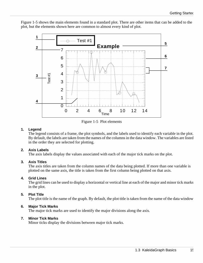
Figure 1-5 shows the main elements found in a standard plot. There are other items that can be addeplot, but the elements shown here are common to almost every kind of plot.
Figure 1-5 Plot elements
1. LegendThe legend consists of a frame, the plot symbols, and the labels used to identify each variable in tBy default, the labels are taken from the names of the columns in the data window. The variables adin the order they are selected for plotting.
2. Axis LabelsThe axis labels display the values associated with each of the major tick marks on the plot.
3. Axis TitlesThe axis titles are taken from the column names of the data being plotted. If more than one variaplotted on the same axis, the title is taken from the first column being plotted on that axis.
4. Grid LinesThe grid lines can be used to display a horizontal or vertical line at each of the major and minor ticksin the plot.
5. Plot TitleThe plot title is the name of the graph. By default, the plot title is taken from the name of the data w
6. Major Tick MarksThe major tick marks are used to identify the major divisions along the axis.
7. Minor Tick MarksMinor ticks display the divisions between major tick marks.
0
1
2
3
4
5
6
7
0 2 4 6 8 10 12 14
ExampleTest #1
Tes
t #1
Time
1
2
3
4
5
6
7
1.3 KaleidaGraph Basics 15
KaleidaGraph
mands.olbar s
king in is
aph.ened bm the
enebmenu
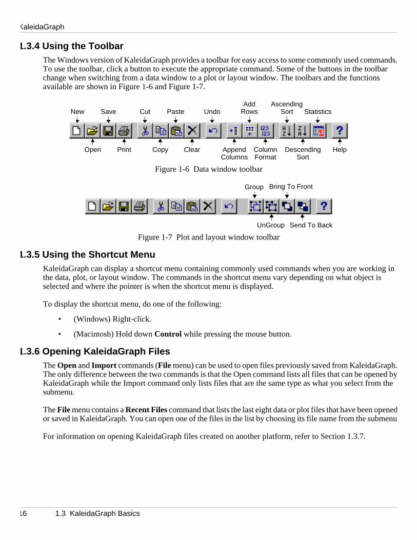
1.3.4 Using the ToolbarThe Windows version of KaleidaGraph provides a toolbar for easy access to some commonly used comTo use the toolbar, click a button to execute the appropriate command. Some of the buttons in the tochange when switching from a data window to a plot or layout window. The toolbars and the functionavailable are shown in Figure 1-6 and Figure 1-7.
Figure 1-6 Data window toolbar
Figure 1-7 Plot and layout window toolbar
1.3.5 Using the Shortcut MenuKaleidaGraph can display a shortcut menu containing commonly used commands when you are worthe data, plot, or layout window. The commands in the shortcut menu vary depending on what objectselected and where the pointer is when the shortcut menu is displayed.
To display the shortcut menu, do one of the following:
• (Windows) Right-click.
• (Macintosh) Hold down Control while pressing the mouse button.
1.3.6 Opening KaleidaGraph FilesThe Open and Import commands (File menu) can be used to open files previously saved from KaleidaGrThe only difference between the two commands is that the Open command lists all files that can be opyKaleidaGraph while the Import command only lists files that are the same type as what you select frosubmenu.
The File menu contains a Recent Files command that lists the last eight data or plot files that have been opdor saved in KaleidaGraph. You can open one of the files in the list by choosing its file name from the su
For information on opening KaleidaGraph files created on another platform, refer to Section 1.3.7.
New
Open
Save Cut Paste UndoAdd
Print Copy Clear Append
Rows
ColumnsColumnFormat
AscendingSort
DescendingSort
Statistics
Help
Group
UnGroup
Bring To Front
Send To Back
16 1.3 KaleidaGraph Basics

Getting Started
below
added.ed
ss
atically
ing on
s that
withs, the gured,ld be
mucile typ
1.3.7 Sharing Files Across PlatformsKaleidaGraph has the ability to share files between the Macintosh and Windows platforms. The tablelists the file name extensions and file types required to do this successfully.
Mac to WindowsTo take a Macintosh file and open it on a Windows computer, the proper file name extension must beFor example, if you created a data file named Results in the Macintosh version, the file needs to be renamResults.QDA to be recognized by the Windows version.
Under OS 9 and earlier, the Preferences dialog contains an option that helps when sharing files acroplatforms. If Add Windows file extensions is selected, the appropriate Windows file name extension is appended to the file name in the Save dialog. Under OS X, the file name extensions are added autom
Windows to MacThe method to open Windows files on a Macintosh depends on what version of KaleidaGraph is runnthe Macintosh. The two cases are listed below:
• Version 3.0.8 or later - No extra steps are necessary. The Open dialog automatically lists filehave the appropriate file name extension and opens them correctly.
• Version 3.0.5 or earlier - For files coming across a network, the file type needs to be modifieda resource editor before KaleidaGraph can read these files correctly. For files stored on diskappropriate file conversion software (for example, PC Exchange) must be installed and confias shown in the preceding table. If the conversion software asks for the creator, QKPT shouentered.
Note: There are two AppleScript droplets available on our web site that make the task of sharing filesheasier. By dragging a file or folder onto these programs, the appropriate file name extension or feis automatically applied.
Kind of File File Name Extension Macintosh File Type
Data file .QDA QDAT
Plot file .QPC QPCT
Macro file .EQN EQNS
Layout file .QPL QPLY
Script file .QSC QSCP
Style file .QST QSTY
1.3 KaleidaGraph Basics 17

KaleidaGraph
e ry,
elp raph tall th
1.3.8 Getting HelpWindows VersionTo get online help, do any of the following:
• Choose Help > Contents.
• Press F1 within any dialog to display context sensitive help.
• Click Help in any dialog that contains a Help button.
• Click the button on the toolbar.
• Choose Start > Programs > KaleidaGraph 3.6 > KGHelp.
Note: If the Help dialog is not displayed, the Help file was not loaded during launch. This occurs if thKGHelp file is renamed or is not in the Help folder (within the KaleidaGraph folder). If necessayou can perform a custom installation to reinstall the Help files.
Macintosh VersionTo get online help, do any of the following:
• Choose Help > KaleidaGraph Help.
• Press the Help key on the keyboard.
• Click Help in any dialog that contains a Help button.
Note: If the Help dialog is not displayed, the KaleidaGraph Help file could not be found or the QuickHprogram was deleted. The KaleidaGraph Help file must be in the same folder as the KaleidaGprogram and it cannot be renamed. If necessary, you can perform a custom installation to reinseHelp files.
18 1.3 KaleidaGraph Basics
Getting Started
Grap If yor search
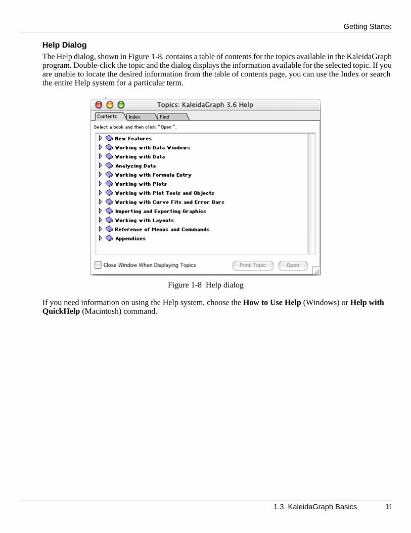
Help DialogThe Help dialog, shown in Figure 1-8, contains a table of contents for the topics available in the Kaleidahprogram. Double-click the topic and the dialog displays the information available for the selected topic.uare unable to locate the desired information from the table of contents page, you can use the Index othe entire Help system for a particular term.
Figure 1-8 Help dialog
If you need information on using the Help system, choose the How to Use Help (Windows) or Help with QuickHelp (Macintosh) command.
1.3 KaleidaGraph Basics 19

KaleidaGraph
types
Save
y the
1.3.9 Setting PreferencesKaleidaGraph provides a Preferences command in the File menu to specify what files are saved when youquit the program. The following dialog is displayed when you choose this command.
Figure 1-9 Preferences dialog
The pop-up menus in the upper section of the dialog control what happens to each of the different filewhen quitting the program. For data and plot files, you can choose to Always save changes or to display a Prompt if there are any unsaved windows. If a data or plot window has not been saved previously, a dialog is displayed.
For the remaining types of files (Layout, Macros, Script, and Style), you can choose whether to displaPrompt dialog if any changes have occurred, Always save, or Never save the changes. For details on the information stored in each of these files, see Appendix B.
Note: The settings for this dialog are saved as part of the Style file. If you choose Never for the Style, you must manually overwrite the default Style file by choosing File > Export > Style.
20 1.3 KaleidaGraph Basics
Getting Started
progra
se
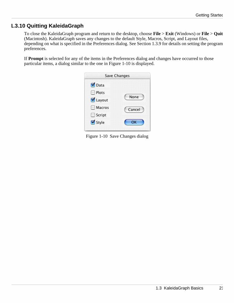
1.3.10 Quitting KaleidaGraphTo close the KaleidaGraph program and return to the desktop, choose File > Exit (Windows) or File > Quit (Macintosh). KaleidaGraph saves any changes to the default Style, Macros, Script, and Layout files, depending on what is specified in the Preferences dialog. See Section 1.3.9 for details on setting the mpreferences.
If Prompt is selected for any of the items in the Preferences dialog and changes have occurred to thoparticular items, a dialog similar to the one in Figure 1-10 is displayed.
Figure 1-10 Save Changes dialog
1.3 KaleidaGraph Basics 21

KaleidaGraph
22 1.3 KaleidaGraph Basics

Guided Tour of KaleidaGraph
Chapter 2
e
tatistics
nd erro
ls, and
d in th user-
n titles
he
This chapter contains four major examples to guide you through the operation of KaleidaGraph. Thesexamples show you how to:
• Create a new data set, change the column titles and format, sort the data, and calculate simple sfor the data.
• Create a Scatter plot, change the display of the variable, use a few plot tools, and add a curve fit arbars.
• Create a Column plot from a saved data set, modify the axes, change the display of the axis labeadd value labels above the columns.
• Display the plots from the preceding examples on the same page using the layout window.
Some optional examples are also included to show you how to perform common operations not covereemain examples. The topics include editing the legend text and frame, using Formula Entry, applying adefined curve fit, and modifying data in a saved plot.
2.1 Generating a Sample Data SetThis example takes you through the process of typing data into the data window, changing the columand format, sorting the data, and calculating statistics on the raw data.
2.1.1 Entering DataThe first step is to type some data into the data window. To do this:
1. Type 4.3 into the first cell of column 0.
2. Press the Enter (Windows), Return (Macintosh), or Down Arrow key to move down to the next cell.
3. Type the values 2.9, 4.8, 3.2, 3.9, 3.5, and 2.3 into column 0. After each value is entered, press tEnter, Return, or Down Arrow key to move down a row.
4. Click the cell at row 0, column 1.
5. Use the same method to type the data values 8.0, 6.2, 9.0, 5.7, 8.8, 7.2, and 4.9 into column 1.
2.1 Generating a Sample Data Set 23

KaleidaGraph
displa
2.1.2 Changing Column Titles and FormatNext we will use the Column Format dialog to change the titles and format for these two columns.
1. Double-click the column title of column 0 (or choose Data > Column Format).
2. Type Time into the field below the listing of column titles.
3. Click the name of the second column (B).
4. Type Test 1 into the field below the listing of column titles.
This dialog can also be used to change the format of the data columns. The following steps change theyof the data so that each value only has one decimal place.
1. Click Time, press Shift, and click Test 1. Both of these entries should be highlighted.
2. From the Format pop-up menu, choose Fixed.
3. From the Decimals pop-up menu, choose 1.
4. Click OK to apply the changes to the data window.
Your data window should resemble the one shown in Figure 2-1.
Figure 2-1 Sample data window
2.1.3 Sorting the DataNow we will sort the data to get the values in ascending order (from low to high).
1. If it is not already selected, click the Time label in the data window to select the entire column.
2. Choose Functions > Ascending Sort.
3. Press Shift and click both the Time and Test 1 entries.
4. Click OK to apply the changes to the data window.
24 2.1 Generating a Sample Data Set

Guided Tour of KaleidaGraph
ow
s how to ve fit,
. By s.
the
2.1.4 Calculating StatisticsThe final step is to calculate a number of standard statistics on one of the data columns.
1. Click the Test 1 label in the data window to select the entire column.
2. Choose Functions > Statistics to display the statistics for the Test 1 data. The Statistics dialogprovides a Copy to Clipboard button to export the results for use in a data, plot, or layout wind
3. Click OK .
At this point, you can proceed to the next example or save your data by choosing File > Save Data.
2.2 Creating and Editing a Scatter PlotThis example uses the data from the preceding example to create a Scatter plot. This example showchange the marker type, size, and color, use the Identify and Data Selection tools, apply a Linear curdisplay the curve fit equation, and add error bars.
2.2.1 Creating a Scatter PlotNow, let’s create a plot using the example data entered in the previous exercise.
1. Choose Gallery > Linear > Scatter. The Variable Selection dialog is displayed. Notice that thename of the data file and its column titles are displayed in this dialog.
2. Select Time as the X variable and Test 1 as the Y variable by clicking the appropriate buttons. Figure 2-2 shows what the Variable Selection dialog should look like at this point.
Figure 2-2 Variable Selection dialog
3. Click New Plot to create a Scatter plot.
The X variable you selected is the independent variable and the Y variable is the dependent variabledefault, the X variable is plotted on the horizontal axis and the Y variable is plotted on the vertical axi
The title of the plot is taken from the name of the data window. The X and Y axis titles are taken fromcolumn titles of the variables being plotted. The Y variable title is also used in the legend.
2.2 Creating and Editing a Scatter Plot 25

KaleidaGraph
he data or.
the lefpaque
e.
d in the
bel
t
urv
pear.
2.2.2 Changing Plot StyleNow that the graph has been created, it can be modified very easily. For example, let’s change how tis represented on the plot. You will use the Plot Style dialog to change the marker type, size, and col
1. Triple-click the marker displayed in the legend (or choose Plot > Plot Style).
2. Select a different marker to represent the variable on the plot. The markers are displayed ontside of the dialog. The first six markers in the left column are transparent; all of the others are o
3. Change the value in the Marker Size field to 18 and select a different color from the color palett
4. Click OK and the plot is redrawn to reflect the changes that have been made.
2.2.3 Using the Identify ToolNow we will use the Identify tool ( ) on the toolbox to display the coordinates of the data.
1. Select the Identify tool by either clicking it or pressing I on your keyboard.
2. Once the tool is selected, click one of the data points. The X and Y coordinates are displayeupper-left corner of the plot window.
It is also possible to leave the coordinates directly on the plot. To do this:
• Press Alt (Windows) or Option (Macintosh) as you release the mouse button. This places a lacontaining the coordinates to the right of the point.
2.2.4 Applying a Linear Curve FitYou can quickly and easily fit a curve to a set of data points. To add a curve fit to the plot:
1. Choose Curve Fit > Linear . This displays a dialog to select which variables to fit with the LeasSquares Error method.
2. Select a variable to be fit (in this case Test 1) by clicking its check box.
3. Click OK . The curve fit is calculated and the curve fit line is drawn on the plot. By default, the cefit results will also be displayed on the plot. If the equation is not displayed, turn on Display Equation in the Plot menu.
The position of the equation can be changed using the Selection Arrow.
1. Click the Selection Arrow on the toolbox.
2. Drag the equation to a new position.
3. When the move is complete, click anywhere else in the window and the object handles disap
4. You can use the same technique to move the legend.
26 2.2 Creating and Editing a Scatter Plot

Guided Tour of KaleidaGraph
ues arehe ialog s.
w
ectiomovee
int is
At this point, your plot should resemble Figure 2-3.
Figure 2-3 Sample Scatter plot
2.2.5 Exporting the Results of the Curve FitOnce a curve fit is applied, you can copy the values of the curve fit line to the data window. These valappended after the existing data in your data window. The first column will be a series of X values. Tnumber of X values will be equal to the number of curve fit points specified in the Curve Fit Options d(Format menu). The second column will contain the values from the curve fit at each of these location
1. Reselect Linear from the Curve Fit menu. A Curve Fit Selections dialog appears with a drop-donarrow under View.
2. Click the drop-down arrow and choose Copy Curve Fit to Data Window from the pop-up menu.
3. Click OK to return to the plot window.
2.2.6 Using the Data Selection ToolNow we will use the Data Selection tool ( ) to graphically remove a point from the plot. The Data Selntool operates by enclosing a region of the plot in a polygon. Any data points outside the polygon are redfrom the plot. By pressing Alt (Windows) or Option (Macintosh) as you make the polygon, the data insidthe polygon can be eliminated.
1. Select the Data Selection tool by either clicking it or pressing S on your keyboard.
2. Once the tool is selected, press Alt (Windows) or Option (Macintosh) and create a polygon aroundthe data point in the lower-left corner of the plot window. Once the polygon is complete, the poremoved and the curve fit is recalculated.
3. Double-click the Data Selection tool to return the plot to its original state.
4
5
6
7
8
9
10
2 2.5 3 3.5 4 4.5 5
Data 1
Test 1
y = 1.0205 + 1.7131x R= 0.9255 T
est 1
Time
3.2, 5.7
2.2 Creating and Editing a Scatter Plot 27

KaleidaGraph
moun
is
e
entire
2.2.7 Adding Error BarsThe last modification to the plot will be the addition of error bars. Error bars enable you to illustrate the atof error for the plotted data.
1. Choose Plot > Error Bars to display the Error Bar Variables dialog.
2. Click the check box in the Y Err column to add vertical error bars. The Error Bar Settings dialogdisplayed to choose the type of error.
3. From the pop-up menu, choose Standard Error for the error type. The dialog should look like thone in Figure 2-4.
Figure 2-4 Error Bar Settings dialog
4. Click OK to return to the Error Bar Selection dialog.
5. Click Plot to add the error bars to the plot. The error bars represent the standard error of thedata column.
The finished plot is shown in Figure 2-5.
28 2.2 Creating and Editing a Scatter Plot

Guided Tour of KaleidaGraph
e plot b the
Figure 2-5 Finished Scatter plot
You have just created a customized plot. You can continue on to the next example or you can save thychoosing File > Save Graph. If you save the graph, a copy of the data window is saved with the plot (insame file). The process of opening a saved plot and extracting the data is covered in Section 2.5.4.
4
5
6
7
8
9
10
2 2.5 3 3.5 4 4.5 5
Data 1
Test 1
y = 1.0205 + 1.7131x R= 0.9255
Tes
t 1
Time
3.2, 5.7
2.2 Creating and Editing a Scatter Plot 29
KaleidaGraph
s,
s.
he
2.3 Creating and Editing a Column PlotThis example uses a Column plot to show how to adjust major and minor ticks, axis labels, fill patterncolumn spacing, plot color, and label rotation, in addition to displaying values above the columns.
2.3.1 Opening a Saved Data FileWe will begin this example by opening a saved data set.
1. Choose File > Open.
2. Locate and open the Data folder, which is located in the Examples folder.
3. Double-click the Housing Starts file.
2.3.2 Creating a Column PlotNow, let’s create a plot using this data.
1. Choose Gallery > Bar > Column. The Variable Selection dialog is displayed.
2. Select Month as the X variable and 1966(K) as the Y variable by clicking the appropriate button
3. Click New Plot to create a Column plot.
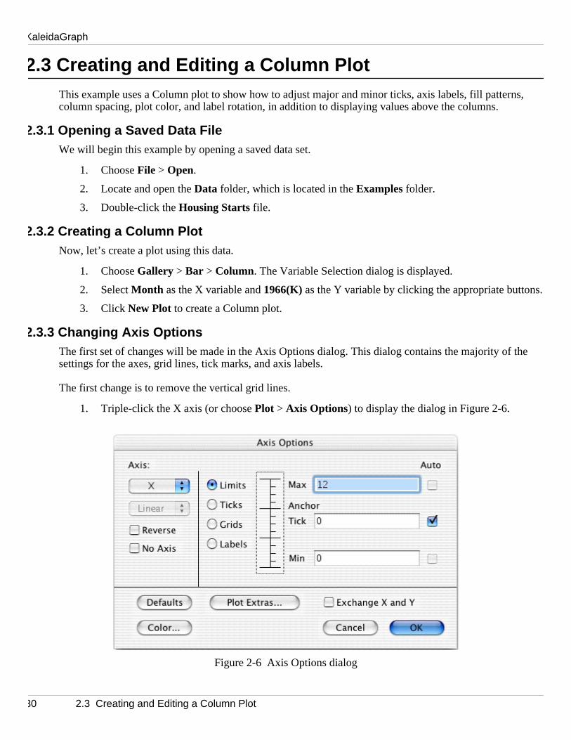
2.3.3 Changing Axis OptionsThe first set of changes will be made in the Axis Options dialog. This dialog contains the majority of tsettings for the axes, grid lines, tick marks, and axis labels.
The first change is to remove the vertical grid lines.
1. Triple-click the X axis (or choose Plot > Axis Options) to display the dialog in Figure 2-6.
Figure 2-6 Axis Options dialog
30 2.3 Creating and Editing a Column Plot

Guided Tour of KaleidaGraph
inor
inor
ialog
s (or
ram
2. Click Grids. The dialog changes to show the options that can be selected for the major and mgrids.
3. Choose None from the pop-up menu to the right of Major .
The next change is to remove the tick marks on the X axis.
1. Click Ticks. The dialog changes to show the options that can be selected for the major and mticks.
2. Choose None from the pop-up menus below both Major and Minor .
The next change also involves the tick marks, but this time on the Y axis.
1. Select the Y axis from the pop-up menu under Axis.
2. Choose Out from the pop-up menus below both Major and Minor .
The last step is to change the maximum Y axis limit from 140 to 160.
1. Click Limits . The dialog changes to show the options that can be selected for the limits.
2. Change the value in the Max field from 140 to 160.
3. Click OK to update the plot with all of the changes that were made while in the Axis Options d
2.3.4 Changing the Fill PatternNow you can change the fill pattern for the columns using the Plot Style dialog.
1. Triple-click the small square in the legend which is filled with the same pattern as the columnchoose Plot > Plot Style).
2. You can now select a different fill pattern for the columns. Click one of the fill patterns and a feappears around that pattern to show that it is selected.
3. Click OK .
2.3.5 Increasing the Column OffsetThe next step is to increase the amount of space between the columns.
1. Choose Format > Plot Extras.
2. Change the Column Offset percentage from 20 to 40%.
3. Click OK to update the plot.
2.3 Creating and Editing a Column Plot 31

KaleidaGraph
ior an
the
e that
e o
lected
At this point, your plot should resemble the one shown in Figure 2-7.
Figure 2-7 Sample Column plot
2.3.6 Changing Plot ColorThe next step is to add some color to the interior of the plot. By default, plots are created without interdbackground colors. To select an interior color:
1. Click any of the four axes to select the plot. Two sets of icons are displayed at the bottom oftoolbox. The first icon displays two overlapping rectangles which control the interior and background color of the plot.
2. Click the rectangle in the foreground and select one of the lighter colors from the color palettappears. The selected color is used to fill the interior of the plot.
2.3.7 Editing Text LabelsThe following steps remove the X axis title, resize the Y axis title, and rotate the X axis labels.
1. Click the X axis title, Month , and press Backspace (Windows) or Delete (Macintosh).
2. Click the Y axis title, 1966 (K). Drag any one of the four object handles to increase the font sizfthe label. It is also possible to change the font size by double-clicking the text label.
3. Double-click one of the X axis labels. Notice that this dialog has its own set of menus.
4. Choose Format > 90 Degree Rotation.
5. Choose Format > Right Justify so that the rotated labels line up evenly.
6. Click OK to return to the plot window.
7. Drag one of the X axis labels closer to the axis. You can also use the arrow keys to move seobjects one pixel at a time in the specified direction (10 pixels if you press Shift while using the arrow keys).
0
20
40
60
80
100
120
140
160
Jan Feb MarchAprilMay June JulyAug Sept Oct Nov Dec
Housing Starts1966 (K)
1966 (K)
Month
32 2.3 Creating and Editing a Column Plot

Guided Tour of KaleidaGraph
to a new
s on a
save
t
of
d an
g you indow.
sin
2.3.8 Adding Value LabelsThe last step is to display the value of each column. To do this, turn on Add Values in the Plot menu. The values are placed at the top of each column. The values can be moved as a group by dragging themlocation.
The Column plot is now complete.
2.4 Laying out Plots for PrintingThis example shows how to use the layout window to place the plots created in the previous examplesingle page.
Note: The following steps assume the two plots from the previous examples are still available. If youdthe plots and quit before reaching this example, use the Open command (File menu) to open these plots. If you do not have them any longer, you can open any two plots from the Plots folder in the Examples folder.
2.4.1 Placing Plots in the LayoutTo place plots into the layout window:
1. Choose Windows > Show Layout > KG Layout . If no layout has been created previously, an empylayout window is displayed.
2. Use the Select Plot command (Layout menu) to select the two plots that were created in the previous examples. At this point, do not worry about their overall placement.
2.4.2 Arranging Plots in the LayoutTo arrange the plots in the layout window:
1. Choose Layout > Arrange Layout. The Arrange Layout dialog allows you to enter the numberrows and columns to divide the layout window into equal sections.
2. The default settings (two rows and one column) are sufficient for this example, so click OK . Noticethat the layout window is divided into two equal sections and the plots are automatically resizedplaced into these sections.
2.4.3 Modifying and Exporting the LayoutIt is possible to display more than just plots in the layout window. The plot tools are available, enablinto add text and other objects to the layout. Various graphic images can be imported into the layout wAlso, a background pattern and frame can be added to the layout using the Set Background command (Layout menu).
The following steps explain how to add a text label to the layout window:
1. Select the Text tool ( ) from the toolbox. You can select this tool by either clicking it or presgT on your keyboard.
2. Click anywhere in the layout window. The Edit String dialog will appear.
2.4 Laying out Plots for Printing 33
KaleidaGraph
light yle, an
nlike rder. ter fee
ntrolled hich is
m thne.
of the s the
tely
sin
t.
size,
ol, yoction
3. Enter some text into this dialog. KaleidaGraph supports fully-stylized text, so feel free to highvarious portions of the text string you have entered and make changes to the font, font size, stdcolor. Any changes you make only affect the selected portion of the text string.
4. Once you are finished making changes, click OK to add the text label to the layout window. You canmove the label to a new position using either the Text tool or the Selection Arrow.
5. You can now print the layout by choosing File > Print Layout .
6. Close the layout window by choosing File > Close.
2.5 Additional ExamplesThis section contains four optional examples to show you some of the finer points of KaleidaGraph. Uthe major examples you completed earlier, you do not have to follow the additional examples in any oYou can select those topics which are relevant to the way you will be using KaleidaGraph to get a grealfor the program.
2.5.1 Editing the LegendThis example shows how to edit the legend frame and text. The attributes of the legend frame are coby the bottom three icons on the toolbox. The steps in this example use the last icon in the toolbox, wdivided into two sections: a Line Style icon on the left and a Line Width icon on the right.
1. Open the Sample Plot file, which is located in the Plots folder in the Examples folder.
2. Click the legend to select it.
3. From the toolbox, click the Line Width icon (the up and down arrows) and choose Hairline froepop-up menu. Notice that the legend frame changes from a shadow box to a hairline width li
4. Now click the Line Style icon (the one to the left of the up and down arrows) and select one dashed lines from the pop-up menu. Notice that the line surrounding the legend now containdashed pattern you selected.
5. Finally, choose None from the Line Style pop-up menu. This removes the legend frame comple
Now we can edit the text inside the legend.
1. Select the Text tool ( ) from the toolbox. You can select this tool by either clicking it or presgT on your keyboard.
2. Double-click any of the three labels inside the legend. A dialog is displayed to modify the tex
3. Delete the text in this dialog and type any information you like. Feel free to change the font, and style as well.
4. Click OK to return to the plot and see the change.
The changes you made only affect this one label. If you use the Selection Arrow instead of the Text toucan change the attributes of all legend items at once. However, you cannot edit the text with the SeleArrow.
34 2.5 Additional Examples

Guided Tour of KaleidaGraph
ata
tions can be
9 and
d lection is
that
can se and
th
2.5.2 Using Formula EntryThis example shows how to use the Formula Entry window, shown in Figure 2-8, to operate on the dwindow. Details on executing a multi-line formula are also included.
Figure 2-8 Formula Entry window
Formula Entry OverviewThe Formula Entry window is a very powerful tool for data analysis. Use Formula Entry to enter equa(functions) that generate and manipulate data in the frontmost data window. The results of a formula placed in a data column, a single cell, or a memory location.
Memory locations and column numbers can be used in formulas. Memory locations range from 0 to 9need to be preceded by an m when used in a formula (m15, m35, and so on).
Column numbers range from 0 to 999 and need to be preceded by a c when used in a formula (c10, c55, anso on). Column numbers are displayed in a box at the top of the column. Please note that when a semade in the data window, the first column in the selection becomes column 0.
The following are a few examples of basic formulas along with a description of each:
c2=c0+c1; Adds the first two columns together and stores the results in column 2.c1=c0/1000; Divides column 0 by 1000 and stores the results in column 1.c2=cos(c0); Calculates the cosine of column 0 and stores the results in column 2.
Executing Individual FormulasLet’s get started by running a few formulas and seeing their effects on the data window. In the steps follow, you can press Enter (Windows) or Return (Macintosh) instead of clicking Run.
1. Choose File > New to display an empty data window.
2. Choose Windows > Formula Entry . By default, the F1 button is selected. The F1–F8 buttons be used to store common formulas, however, we recommend that you leave F1 for general ustore your formulas in F2–F8.
3. Click F2, type c0=index() + 1, and click Run. This creates a series from 1 to 100 in column 0.
4. Click F3, type c1=log(c0), and click Run. This function calculates the logarithm of each value incolumn 0 and stores the results in column 1.
5. Click F4, type c2=c1^2, and click Run. This formula squares each value in column 1 and storeseresults in column 2.
2.5 Additional Examples 35

KaleidaGraph
eroll
multipl
You
ndow:
a
rmul
od, yo
ve fit. to nine
6. Click F5, type cell(0,3)=csum(c2), and click Run. This formula calculates the total sum of the valusin column 2 and stores the result in the cell at row 0, column 3. You need to click the right scarrow to see the result of this formula.
Executing Multi-line FormulasIt is not necessary to enter and execute each formula individually. KaleidaGraph has a method to enter eformulas and execute them all at once.
To the left of the F1 button is a Posted Note button ( ). Clicking this button displays a text editor.can enter multiple formulas into the editor and run them all at once by clicking Run. The formulas must be onseparate lines and each must be terminated with a semicolon.
Let’s try using the same formulas from before, but this time executing them using the Posted Note wi
1. Choose File > New to display an empty data window.
2. Choose Windows > Formula Entry .
3. Click the Posted Note button in the Formula Entry window to display a text editor.
4. Type the following formulas into the Posted Note window. Note that each formula ends with semicolon and appears on a separate line.
c0=index() + 1;c1=log(c0);c2=c1^2;cell(0,3)=csum(c2);
5. After the formulas are entered, choose File > Close to return to the Formula Entry window. A message is displayed in the Formula Entry window telling you to click Run to execute the FoaPosted Note.
6. Click Run to execute all of the formulas at once.
As you can see, this is a very convenient method to execute multiple formulas at once. Using this methucan save the formulas as a text file that can be opened at a later time within the Posted Note dialog.
2.5.3 Applying a General (user-defined) Curve FitThis example takes you through the process of opening a saved plot and applying a user-defined curKaleidaGraph’s General curve fit is based on the Levenberg-Marquardt algorithm. You can solve up unknown parameters during the fitting process.
Opening a Saved PlotWe will start by opening a saved plot.
1. Choose File > Open.
2. Locate and open the Plots folder, which is located in the Examples folder.
3. Double-click the Inhibition Plot file.
36 2.5 Additional Examples
Guided Tour of KaleidaGraph
of
nown
l
on witrror. Th
hide
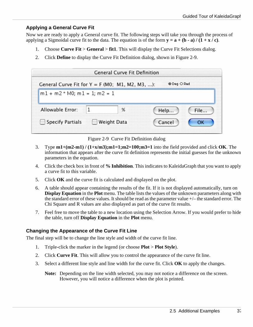
Applying a General Curve FitNow we are ready to apply a General curve fit. The following steps will take you through the process applying a Sigmoidal curve fit to the data. The equation is of the form y = a + (b - a) / (1 + x / c).
1. Choose Curve Fit > General > fit1 . This will display the Curve Fit Selections dialog.
2. Click Define to display the Curve Fit Definition dialog, shown in Figure 2-9.
Figure 2-9 Curve Fit Definition dialog
3. Type m1+(m2-m1) / (1+x/m3);m1=1;m2=100;m3=1 into the field provided and click OK . The information that appears after the curve fit definition represents the initial guesses for the unkparameters in the equation.
4. Click the check box in front of % Inhibition . This indicates to KaleidaGraph that you want to appya curve fit to this variable.
5. Click OK and the curve fit is calculated and displayed on the plot.
6. A table should appear containing the results of the fit. If it is not displayed automatically, turnDisplay Equation in the Plot menu. The table lists the values of the unknown parameters alonghthe standard error of these values. It should be read as the parameter value +/– the standard eeChi Square and R values are also displayed as part of the curve fit results.
7. Feel free to move the table to a new location using the Selection Arrow. If you would prefer tothe table, turn off Display Equation in the Plot menu.
Changing the Appearance of the Curve Fit LineThe final step will be to change the line style and width of the curve fit line.
1. Triple-click the marker in the legend (or choose Plot > Plot Style).
2. Click Curve Fit. This will allow you to control the appearance of the curve fit line.
3. Select a different line style and line width for the curve fit. Click OK to apply the changes.
Note: Depending on the line width selected, you may not notice a difference on the screen. However, you will notice a difference when the plot is printed.
2.5 Additional Examples 37

KaleidaGraph
nally,he plot.
the
and
e
2.5.4 Modifying Data in a Saved PlotThis example shows how to modify a data point in a saved plot and have the plot and any curve fits automatically updated.
Extracting the DataTo get started, we need to open a saved plot and extract the data. To do this:
1. Choose File > Open and open the Sample Plot file (located in the Plots folder, within the Examplesfolder).
2. With the plot frontmost, choose Plot > Extract Data. The original data used to create the plot is displayed. The title of the window begins with the same name as the original data file. Additioa date and time stamp is appended to the name, identifying when the data was archived in t
Changing the Data and Updating the PlotNow we can make changes to the data and have the plot updated.
1. Turn on Auto Link in the Plot menu. When this command is active, you can make changes todata and have the plot automatically updated after each individual change.
2. Change the value in the first row of column 1 from 78.5 to 100.
3. Use one of the arrow keys to move to another cell to activate the Auto Link feature. The plotcurve fit are automatically updated to reflect the modified data value.
Changing Multiple Data PointsIf you need to add or modify multiple data points, it may be more efficient to use the Update Plot command(Plot menu) because Auto Link causes the plot to update after each change. In this case, turn off Auto Link ,make any changes to the data, and choose the Update Plot command. The plot is updated to reflect all of thchanges at once.
38 2.5 Additional Examples

Working with Data Windows
Chapter 3
n view
alic.
10
he fron
This chapter explains how to:
• Create a new data window.
• Use the keyboard to move through the data window.
• Select rows, columns, and a range of cells in the data window.
• Add, insert, and delete rows and columns.
• Edit column titles.
• Change the data format and width of columns.
• Use the Posted Note feature to make notes about the data.
3.1 Hiding, Displaying, and Closing Data WindowsA maximum of 160 data windows can be open at any one time, subject to memory limitations. You caa list of all open data windows by choosing Windows > Show Data. Data windows that are currently displayed on the screen have their names in normal text. Names of hidden data windows appear in it
3.1.1 Creating a New Data WindowA blank data window can be created by choosing File > New. Any defaults that have been set using the Column Format command are used to create the new window. By default, data windows are createdcolumns by 100 rows in size and named Data 1, Data 2, and so on.
3.1.2 Changing the Active WindowTo make a data window active, click anywhere in the desired data window or choose Windows > Show Dataand select its name.
3.1.3 Hiding Data WindowsA data window can be hidden by choosing Windows > Hide Window and selecting its name. The next window in the list becomes active.
3.1.4 Displaying Data WindowsA hidden data window can be displayed using the Show Data command (Windows menu). The names of hidden data windows appear in italic. Select the name of the desired data window and it is brought to tt
3.1 Hiding, Displaying, and Closing Data Windows 39

KaleidaGraph
e.
e
With thw, use
indow
e of th effects
3.1.5 Closing Data WindowsYou can use the Close All Data command (Windows menu) to close all of the open data windows at oncIndividual data windows can be closed by choosing File > Close or clicking the close box of each window. Adialog may be displayed, asking if you want to save the data window before closing.
Note: If you do not want to save the data, this dialog can be avoided by pressing Shift while either clickingthe close box or choosing File > Close/NoSave.
3.2 Moving Around the Data WindowThere are three methods available for moving around in the data window. You can use the mouse, thkeyboard, or the Go To Cell command.
3.2.1 Using the MouseOne of the easiest and most common methods to move around the data window is to use the mouse.emouse, you can move to any cell in the data window. To move to a different section of the data windothe horizontal and vertical scroll bars.
You can also use the Home button ( ) in the upper-left corner of the data window to return the wto its origin (row 0, column 0). This is useful for quickly returning to the start of the data window.
3.2.2 Using the KeyboardThere are a number of keys on the keyboard that let you move from one cell to another. When the edgeviewing area is reached, the data window scrolls to display the next row or column. The keys and theirare listed in the following table.
Key Direction
Left/Right Arrow Move one cell left/right.
Up/Down Arrow Move one cell up/down.
Tab Move one cell to the right.
Shift+Tab Move one cell to the left.
Return Move down one cell.
Shift+Return Move up one cell.
Enter Windows: Same as the Return key.Macintosh: Move one cell in the same direction as the last move.
Page Up/Down Move one window view up/down.
Home Move to top of column.
End Move to bottom of column.
40 3.2 Moving Around the Data Window

Working with Data Windows
g l. Whe
ve to
in th
dow.
to
ll
3.2.3 Using the Go To Cell CommandThe Go To Cell command (Data menu) can be used to view a specific cell in the data window. Choosinthis command displays the dialog in Figure 3-1 to enter the row and column numbers of the desired celnyou click OK , the data window automatically scrolls to make that cell position visible.
Figure 3-1 Go To Cell dialog
3.3 Switching Between Overwrite and Insert ModeKaleidaGraph provides two commands, Overwrite Mode and Insert Mode, that control what happens whenyou try to edit or replace a data value. The active mode is preceded by a check mark in the Data menu.
If Overwrite Mode is active, cells are automatically selected when using the mouse or keyboard to moacell. Typing data into the current cell replaces any existing data.
If Insert Mode is active, clicking a cell does not automatically select the cell. Instead, a cursor is placedecell to edit the current value. To select a cell in Insert Mode, double-click the active cell.
3.4 Making Selections in the Data WindowThis section explains how to select rows, columns, a range of cells, and all of the cells in the data win
3.4.1 Selecting RowsA single row can be selected by clicking its row number.
To select a range of rows, do one of the following:
• Click the number of the first or last row that you want and drag to complete the selection.
• Click the first row to be included, press Shift, and click the last row. You can use the scroll barsmove to the last row.
3.4.2 Selecting ColumnsA single column can be selected by clicking the column title.
To select a range of columns, do one of the following:
• Click the column title of the first or last column and drag to complete the selection.
• Click the first column to be included, press Shift, and click the last column. You can use the scrobars to move to the last column.
3.3 Switching Between Overwrite and Insert Mode 41

KaleidaGraph
ells are
mber o
ed up to
3.4.3 Selecting a Range of CellsTo select a range of cells, drag the mouse until all of the cells you want are selected. If some of the cnot visible, keep dragging and the data window will scroll automatically.
To select a large block of data, click the first cell of the block, press Shift, and click the cell in the opposite corner of the block. You can use the scroll bars to move to the second cell.
3.4.4 Selecting the Entire WindowTo select all of the cells in the data window, choose Edit > Select All.
3.5 Adding and Deleting Rows and ColumnsBy default, data windows are created with 10 columns and 100 rows. It is very easy to increase the nufrows and columns in the data window.
3.5.1 Adding Rows and ColumnsAdding RowsTo add more rows to the data window, choose Data > Add Rows. This command displays the dialog in Figure 3-2 to enter the number of rows to be added to the data window. The number entered is roundthe next multiple of 100.
Figure 3-2 Add Rows dialog
Note: If the active cell is in the last row of the data window, pressing the Enter (Windows), Return (Macintosh), or Down Arrow key automatically adds 100 rows to the data window.
Adding ColumnsTo add more columns to the data window, do one of the following:
• Choose Data > Append Columns and enter the number of columns to be appended to the datawindow.
• Press the Right Arrow key (if the active cell is in the last column of the data window).
• Click the Add button in the Column Format dialog (Data menu).
42 3.5 Adding and Deleting Rows and Columns

Working with Data Windows
ange o
ata
3.5.2 Inserting Rows and ColumnsInserting RowsRows can be inserted anywhere in the data window. A row can be inserted in a single column or in a rfcolumns.
To insert a row:
1. Make a selection in the data window. The row is inserted above the selection.
2. Choose Data > Insert Row. A row of blank cells is inserted into the data window.
Inserting ColumnsTo insert a column into the data window:
1. Select a column in the data window.
2. Choose Data > Insert Column. A blank column is inserted before the selected column in the dwindow.
Columns can also be inserted by pressing Alt (Windows) or Option (Macintosh) and clicking a column. A new column is inserted before the selected column.
3.5.3 Deleting Rows and ColumnsDeleting RowsRows can be deleted from the data window by making a selection and choosing Data > Delete Row. The selection is deleted and the remaining data shifts up to take the place of the deleted data.
Deleting ColumnsColumns can be deleted from the data window by making a selection and choosing Data > Delete Column. The selection is deleted and the remaining data shifts over to take the place of the deleted data.
3.5 Adding and Deleting Rows and Columns 43
KaleidaGraph
s six a typee data own in
s
lumn is
acters to use
or lin creatfigures.
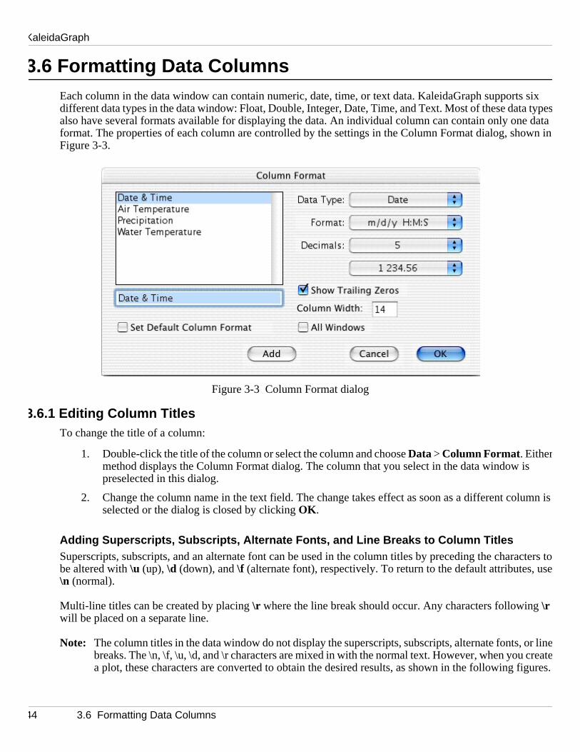
3.6 Formatting Data ColumnsEach column in the data window can contain numeric, date, time, or text data. KaleidaGraph supportdifferent data types in the data window: Float, Double, Integer, Date, Time, and Text. Most of these datsalso have several formats available for displaying the data. An individual column can contain only onformat. The properties of each column are controlled by the settings in the Column Format dialog, shFigure 3-3.
Figure 3-3 Column Format dialog
3.6.1 Editing Column TitlesTo change the title of a column:
1. Double-click the title of the column or select the column and choose Data > Column Format. Eithermethod displays the Column Format dialog. The column that you select in the data window ipreselected in this dialog.
2. Change the column name in the text field. The change takes effect as soon as a different coselected or the dialog is closed by clicking OK .
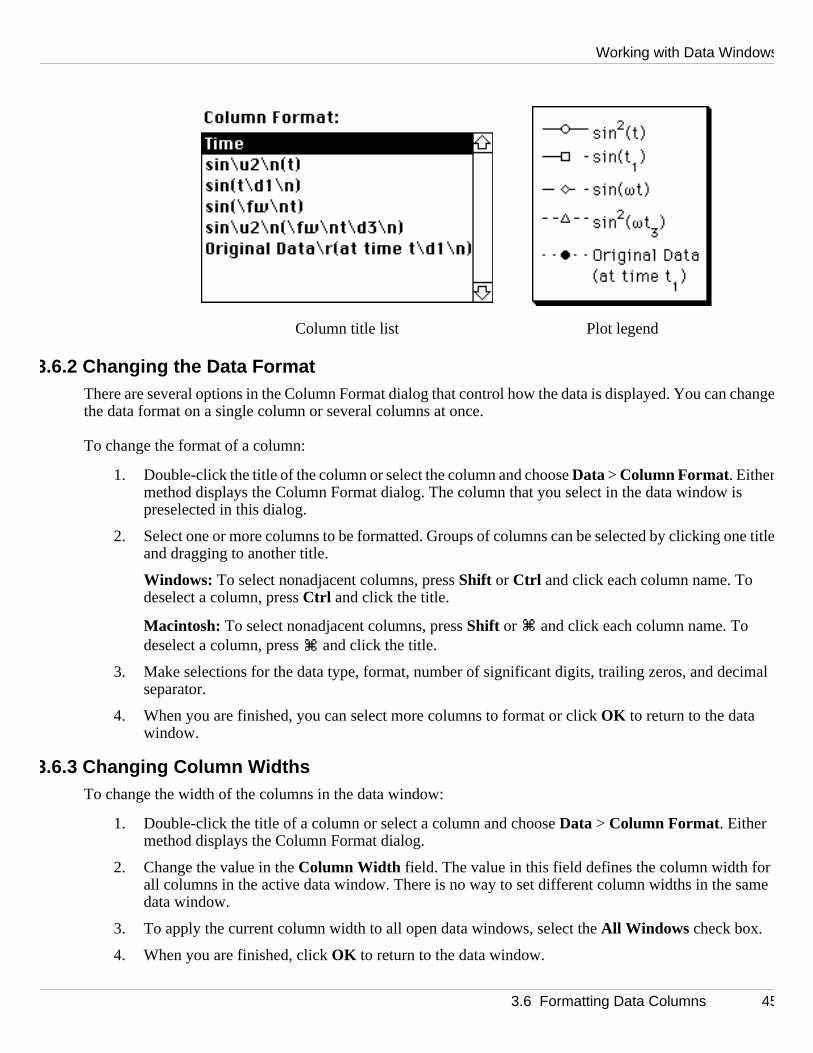
Adding Superscripts, Subscripts, Alternate Fonts, and Line Breaks to Column TitlesSuperscripts, subscripts, and an alternate font can be used in the column titles by preceding the charbe altered with \u (up), \d (down), and \f (alternate font), respectively. To return to the default attributes, \n (normal).
Multi-line titles can be created by placing \r where the line break should occur. Any characters following\r will be placed on a separate line.
Note: The column titles in the data window do not display the superscripts, subscripts, alternate fonts,ebreaks. The \n, \f, \u, \d, and \r characters are mixed in with the normal text. However, when youea plot, these characters are converted to obtain the desired results, as shown in the following
44 3.6 Formatting Data Columns
Working with Data Windows
chang
s
ne titl
imal
r ame
3.6.2 Changing the Data FormatThere are several options in the Column Format dialog that control how the data is displayed. You canethe data format on a single column or several columns at once.
To change the format of a column:
1. Double-click the title of the column or select the column and choose Data > Column Format. Eithermethod displays the Column Format dialog. The column that you select in the data window ipreselected in this dialog.
2. Select one or more columns to be formatted. Groups of columns can be selected by clicking oeand dragging to another title.
Windows: To select nonadjacent columns, press Shift or Ctrl and click each column name. To deselect a column, press Ctrl and click the title.
Macintosh: To select nonadjacent columns, press Shift or and click each column name. To deselect a column, press and click the title.
3. Make selections for the data type, format, number of significant digits, trailing zeros, and decseparator.
4. When you are finished, you can select more columns to format or click OK to return to the data window.
3.6.3 Changing Column WidthsTo change the width of the columns in the data window:
1. Double-click the title of a column or select a column and choose Data > Column Format. Either method displays the Column Format dialog.
2. Change the value in the Column Width field. The value in this field defines the column width foall columns in the active data window. There is no way to set different column widths in the sdata window.
3. To apply the current column width to all open data windows, select the All Windows check box.
4. When you are finished, click OK to return to the data window.
Column title list Plot legend
3.6 Formatting Data Columns 45

KaleidaGraph
set. The
.
3.7 Making Notes about the DataEach data window in KaleidaGraph provides a text editor where you can make notes about the data text editor is displayed by either choosing Data > Posted Note or clicking the Posted Note button ( ) inthe data window. This information is unique for each data window and is saved as part of the data file
46 3.7 Making Notes about the Data

Working with Data
Chapter 4
re you d the
e:
This chapter explains how to:
• Enter data.
• Generate a data series.
• Import text files.
• Cut, copy, paste, and clear data.
• Sort data.
• Exchange rows and columns.
• Execute macros.
• Save and print data.
4.1 Entering DataYou can enter numeric, date, time, or text data into the data window. Before you enter data, make suknow how to move around the data window and how to change the format of a column. Moving aroundata window is covered in Section 3.2; changing the data format is covered in Section 3.6.
4.1.1 Entering Numeric DataThe Column Format dialog (Data menu) provides three data types for displaying numeric data. They ar
• Float - Accurate for numbers containing up to seven digits.
• Double - Accurate for numbers containing up to 16 digits.
• Integer - Displays the numbers as integers.
4.1 Entering Data 47

KaleidaGraph
eep lude:
.
nable ta froat are spaces.
To enter numeric data:
1. Double-click the title of a column or select a column and choose Data > Column Format. Verify that the correct data type and format are selected for the column.
2. After you leave the Column Format dialog, use the mouse or arrow keys to select a cell.
3. Type the data value. If you make a mistake, press Backspace (Windows) or Delete (Macintosh) to remove incorrect characters.
Note: To enter numbers in scientific notation, enter the number, followed by an e and the power (for example, 1.23e–4).
4. Press Enter (Windows) or Return (Macintosh) to move down one row, or use the arrow keys tomove around the data window.
5. Repeat steps 3 and 4 until all of the data is entered.
Note: If KaleidaGraph detects any characters that are not associated with the selected data type, a bsounds when you move to the next cell. Examples of incorrect characters for numeric data inctext, multiple decimal points, and separators for date and time numbers.
4.1.2 Entering Date or Time DataTo enter date or time data:
1. Double-click the title of a column or select a column and choose Data > Column Format.
2. Choose either Date or Time from the Data Type pop-up menu.
3. Choose the desired format from the Format pop-up menu and click OK .
4. Use the mouse or arrow keys to select a cell.
5. Type the date or time data. If you make a mistake, press Backspace (Windows) or Delete (Macintosh) to remove incorrect characters.
Note: When entering two digit years less than 40, the Promote 2 digit dates less than 40 option inthe Preferences dialog determines whether the dates are interpreted as 19xx or 20xx
6. Press Enter (Windows) or Return (Macintosh) to move down one row, or use the arrow keys tomove around the data window.
7. Repeat steps 5 and 6 until all of the data is entered.
If you import date or time data from a file, the format must closely match the actual format shown to eKaleidaGraph to recognize the column properly. However, if you are typing the data or pasting the damthe Clipboard (to a column that has been set to a date or time format), variations from the exact formallowed. Valid separators for the date and time formats include: slashes (/), colons (:), commas, and
When importing dates from another program, the Default Date Format setting in the Preferences dialog (Filemenu) determines how the dates are interpreted by KaleidaGraph.
48 4.1 Entering Data

Working with Data
ake a
aph
e first dent
n
otted.
that coms whic
ery muc
series
date o
4.1.3 Entering Text DataTo enter text data:
1. Double-click the title of a column or select a column and choose Data > Column Format.
2. Choose Text from the Data Type pop-up menu and click OK .
3. Use the mouse or arrow keys to select a cell.
4. Enter the text data. A maximum of 50 characters can be entered for each text label. If you mmistake, press Backspace (Windows) or Delete (Macintosh) to remove incorrect characters.
5. Press Enter (Windows) or Return (Macintosh) to move down one row, or use the arrow keys tomove around the data window.
6. Repeat steps 4 and 5 until all of the data is entered.
Note: Any data that is entered into a Text column appears left-justified.
4.1.4 Missing ValuesThere may be times when data values are missing in a series of data. In the data window, KaleidaGrrepresents a missing data value with an empty cell, regardless of the data type.
When plotting, if the independent variable (X) contains missing values, KaleidaGraph searches for thand last cells that contain data and plots all values in between, ignoring any empty cells. If the depenvariable (Y) contains missing values, the empty cells are ignored when plotting.
There is an option in the Plot Extras dialog (Format menu) that controls how missing values are treated iLine, Double Y, Double X, Double XY, High/Low, Step, X-Y Probability, and Polar plots. When Missing Data Breaks is selected, a missing data point in an X or Y variable causes a break in the line being plOtherwise, the line is continuous and the missing data points are ignored.
4.2 Generating a Data SeriesThere are several methods that can be used to generate a series of data. Some of the default macrosewith KaleidaGraph can be used to create a data series. The Formula Entry window contains commandhcan also be used to place a series into a column. The only problem is these methods do not give you vhcontrol over the type of series that is generated.
The one method that does give you complete control is the Create Series command from the Functions menu.This command allows you to specify an initial value, an increment, a multiplier, and a final value for the
You can create a numeric series in any column that contains a Float, Double, or Integer data format. Artime series can be created in any column that contains a Date or Time format.
Note: It is not possible to generate a series in a Text column.
4.2 Generating a Data Series 49

KaleidaGraph
he
ad datta must
dialo
To create a series:
1. Select a column or a range of columns in the data window.
2. Choose Functions > Create Series. A dialog similar to one of the following appears, based on tformat of the column.
Figure 4-1 Create Series dialog (Numeric format)
Figure 4-2 Create Series dialog (Date format)
3. Enter values into the appropriate fields of the dialog and click OK to generate the series.
4.3 Importing Text FilesKaleidaGraph can open text files that are formatted in a number of different ways. This allows you to reacreated in another program and use that data in KaleidaGraph. The only requirements are that the dabe saved as a text file and the information must be arranged in a repeating pattern.
4.3.1 Text File Input Format DialogWhenever you select a text file to be read into KaleidaGraph, the dialog in Figure 4-3 is displayed. Thisgallows you to:
• Preview the file.
• Select the delimiter.
50 4.3 Importing Text Files
Working with Data
g tex
eparate
ecial
betwee
esent,
re
• Indicate the number of delimiters between columns.
• Specify the number of lines to skip at the beginning of a file.
• Select whether or not to read titles into the data window.
Note: If you are using the Macintosh version of KaleidaGraph, this dialog is not displayed when openintfiles saved from KaleidaGraph. To display the dialog, press Option when opening these text files.
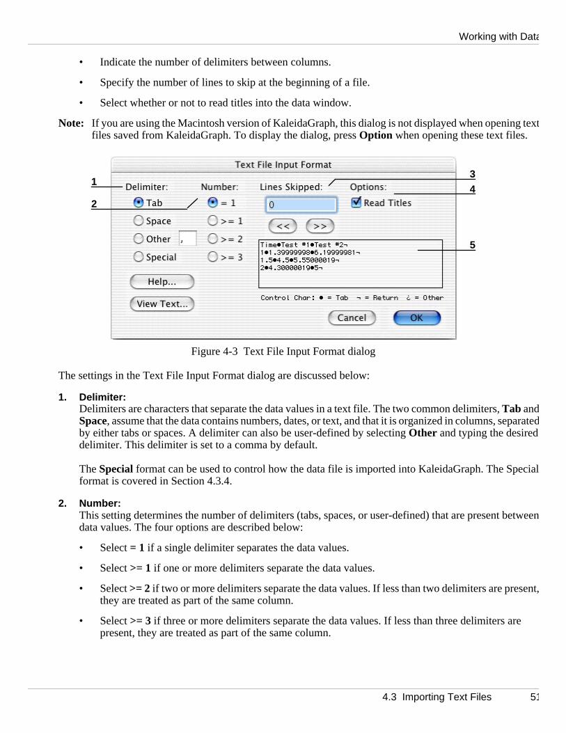
Figure 4-3 Text File Input Format dialog
The settings in the Text File Input Format dialog are discussed below:
1. Delimiter:Delimiters are characters that separate the data values in a text file. The two common delimiters, Tab andSpace, assume that the data contains numbers, dates, or text, and that it is organized in columns, sdby either tabs or spaces. A delimiter can also be user-defined by selecting Other and typing the desired delimiter. This delimiter is set to a comma by default.
The Special format can be used to control how the data file is imported into KaleidaGraph. The Spformat is covered in Section 4.3.4.
2. Number:This setting determines the number of delimiters (tabs, spaces, or user-defined) that are present ndata values. The four options are described below:
• Select = 1 if a single delimiter separates the data values.
• Select >= 1 if one or more delimiters separate the data values.
• Select >= 2 if two or more delimiters separate the data values. If less than two delimiters are prthey are treated as part of the same column.
• Select >= 3 if three or more delimiters separate the data values. If less than three delimiters apresent, they are treated as part of the same column.
134
5
2
4.3 Importing Text Files 51

KaleidaGraph
adjustu are
umn
of th
ced in
that uses
he
3. Lines Skipped:This setting determines the number of lines at the beginning of the file which are skipped before interpreting the rest of the data. As this number changes, the data displayed in the preview windowsto reflect the change. The skipped lines are automatically placed into the Posted Note, unless yomerging a text file with a data set that already contains information in the Posted Note.
4. Options:When the Read Titles check box is selected, the first line in the preview window is used for the coltitles.
5. Preview WindowThis window displays 40 characters from the first four lines of the text file. To see a larger sampleefile, click View Text.
4.3.2 Importing Missing Data PointsMissing data points can be entered from text files. If =1 is selected for the Number setting in the Text File Input Format dialog, whenever KaleidaGraph detects two consecutive delimiters, an empty cell is plathe data window.
A period can also be used to represent an empty data cell. There is a mainframe program called SAS the period as a default character for empty data cells.
4.3.3 Example - Reading Basic FormatsThis section shows how to import a simple tab-delimited text file. One of the text files that comes withKaleidaGraph is used as an example.
To import this example data set:
1. Choose File > Open.
2. Locate and open the Data folder, which is located in the Examples folder.
3. Double-click the file Text Example. When KaleidaGraph determines that the file is a text file, tdialog in Figure 4-4 appears.
Figure 4-4 Text File Input Format dialog
52 4.3 Importing Text Files
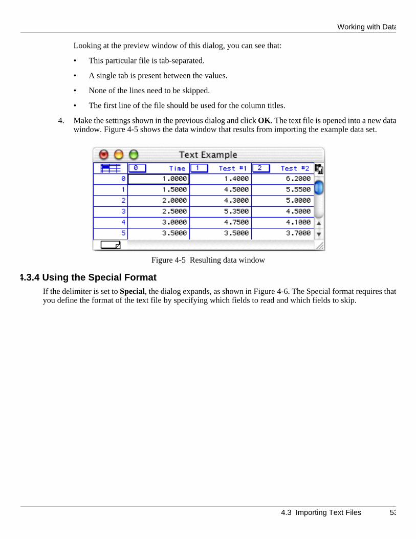
Working with Data
tha
Looking at the preview window of this dialog, you can see that:
• This particular file is tab-separated.
• A single tab is present between the values.
• None of the lines need to be skipped.
• The first line of the file should be used for the column titles.
4. Make the settings shown in the previous dialog and click OK . The text file is opened into a new datawindow. Figure 4-5 shows the data window that results from importing the example data set.
Figure 4-5 Resulting data window
4.3.4 Using the Special FormatIf the delimiter is set to Special, the dialog expands, as shown in Figure 4-6. The Special format requirestyou define the format of the text file by specifying which fields to read and which fields to skip.
4.3 Importing Text Files 53
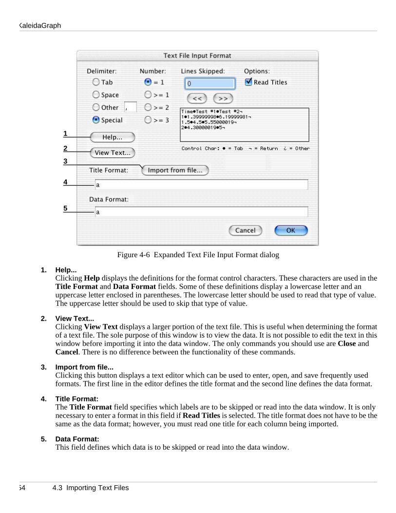
KaleidaGraph
in th
of value.
main this
sed rmat.
only th
Figure 4-6 Expanded Text File Input Format dialog
1. Help...Clicking Help displays the definitions for the format control characters. These characters are usedeTitle Format and Data Format fields. Some of these definitions display a lowercase letter and an uppercase letter enclosed in parentheses. The lowercase letter should be used to read that typeThe uppercase letter should be used to skip that type of value.
2. View Text...Clicking View Text displays a larger portion of the text file. This is useful when determining the fortof a text file. The sole purpose of this window is to view the data. It is not possible to edit the text window before importing it into the data window. The only commands you should use are Close and Cancel. There is no difference between the functionality of these commands.
3. Import from file...Clicking this button displays a text editor which can be used to enter, open, and save frequently uformats. The first line in the editor defines the title format and the second line defines the data fo
4. Title Format:The Title Format field specifies which labels are to be skipped or read into the data window. It is necessary to enter a format in this field if Read Titles is selected. The title format does not have to be esame as the data format; however, you must read one title for each column being imported.
5. Data Format:This field defines which data is to be skipped or read into the data window.
1
2
3
4
5
54 4.3 Importing Text Files

Working with Data
ext file
he
ialog
be ime
4.3.5 Example - Reading Special FormatsThis section shows an example of importing a text file that contains unwanted data values. One of the tsthat comes with KaleidaGraph is used as an example.
To import this example data set:
1. Choose File > Open.
2. Locate and open the Data folder, which is located in the Examples folder.
3. Double-click the file Measurements. When KaleidaGraph determines that the file is a text file, tText File Input Format dialog appears.
4. Click the Special button. The dialog expands so you can enter the title and data formats. The dshould look like Figure 4-7 at this point.
Figure 4-7 Expanded Text File Input Format dialog
Looking at the preview window of this dialog, you can see that:
• The file begins with an unusable line which must be skipped.
• There is a title line containing three labels.
• The data is spread across six columns. Three of the columns contain labels and should skipped. The other three contain values which should be read as one fixed width field (Tvalues) and two variable width fields (Temperature and Volume values).
4.3 Importing Text Files 55

KaleidaGraph
e 4-8
ad int
5. Using the above information, you can now specify the format of the titles and the data. Figurshows how the dialog should appear after making the following selections.
• Lines Skipped should be 1 to skip the first line.
• Read Titles should be selected to read in the column titles.
• The Title Format should be either a a a or 3(a). Either one of these formats reads in three labels, separated by white space.
• The Data Format should be either A f3 A v A v or A f3 2(A v). Using either one of these formats, the three columns of labels are skipped and only the three columns of data are reothe data window.
Figure 4-8 Finished Text File Input Format dialog
6. Click OK to import the text file. The resulting data window is shown in Figure 4-9.
56 4.3 Importing Text Files
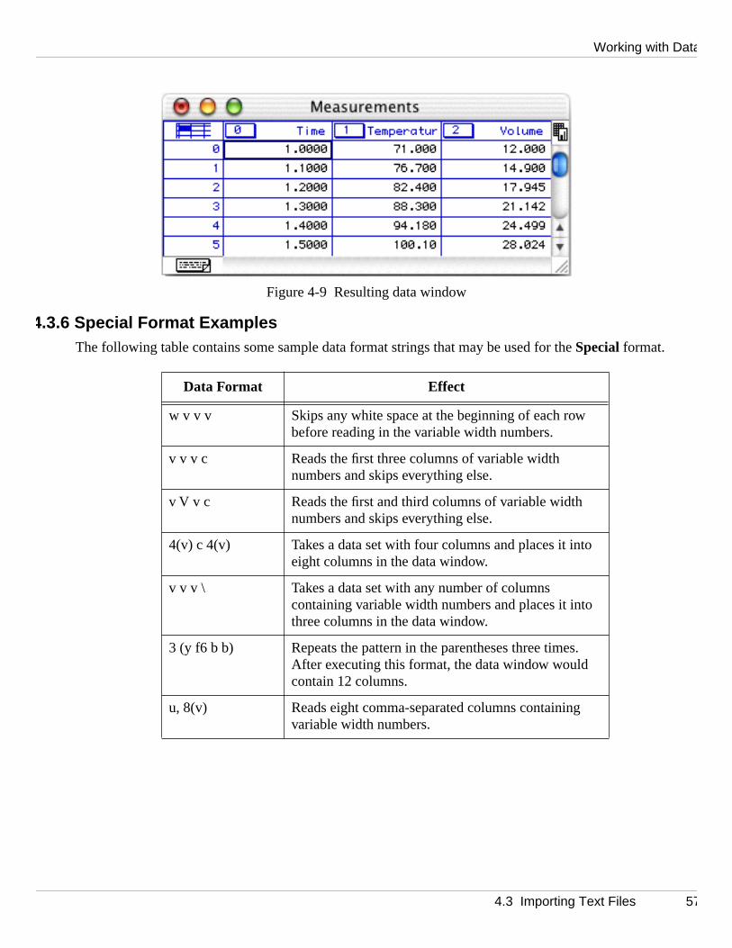
Working with Data
Figure 4-9 Resulting data window
4.3.6 Special Format ExamplesThe following table contains some sample data format strings that may be used for the Special format.
Data Format Effect
w v v v Skips any white space at the beginning of each row before reading in the variable width numbers.
v v v c Reads the first three columns of variable width numbers and skips everything else.
v V v c Reads the first and third columns of variable width numbers and skips everything else.
4(v) c 4(v) Takes a data set with four columns and places it into eight columns in the data window.
v v v \ Takes a data set with any number of columns containing variable width numbers and places it into three columns in the data window.
3 (y f6 b b) Repeats the pattern in the parentheses three times. After executing this format, the data window would contain 12 columns.
u, 8(v) Reads eight comma-separated columns containing variable width numbers.
4.3 Importing Text Files 57
KaleidaGraph
sing
ntta are
e Texram.
mar
g th
tents,
to th
ard.
4.4 Cutting, Copying, Pasting, and Clearing DataThere are several commands in the Edit menu that can be used to edit the contents of the data window. Uthese commands, you can cut, copy, paste, and clear data selections.
4.4.1 Binary Mode/Text Mode SettingThis command controls whether the Cut and Copy commands use binary or text format to copy large amousof data to the Clipboard. When copying 10000 cells or less, a binary and text representation of the dacopied to the Clipboard. This occurs regardless of which mode is currently active.
Binary editing is much faster than text editing and allows you to quickly move large amounts of data. Ustmode if you need to copy more than 10000 cells and paste them into the plot window or another prog
To view the active mode, click the Edit menu. The active mode is displayed in the menu and has a check kin front of it. To switch between modes, choose the active mode.
4.4.2 Cutting DataChoose Edit > Cut to remove the data selection from the window and place it on the Clipboard, replacineprevious contents, if any.
4.4.3 Copying DataChoose Edit > Copy to place a copy of the data selection on the Clipboard, replacing the previous conif any.
4.4.4 Pasting DataChoose Edit > Paste to place the Clipboard’s contents into the data window. You can also paste data ineplot window, layout window, or another program.
4.4.5 Clearing DataChoose Edit > Clear to delete all of the cells in the selection without disturbing the contents of the ClipboTo clear a cell’s contents without deleting the cell, use the Clear Data command, the Backspace key (Windows), or the Delete key (Macintosh).
4.4.6 Including Column Titles when Editing DataTo include the column titles when editing, press Shift while choosing the Cut, Copy, Paste, or Clear command from the Edit menu.
58 4.4 Cutting, Copying, Pasting, and Clearing Data
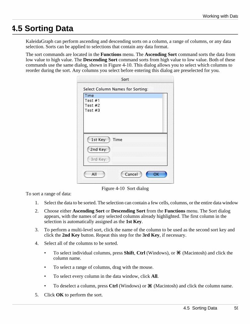
Working with Data
data
e s to
window
and
4.5 Sorting DataKaleidaGraph can perform ascending and descending sorts on a column, a range of columns, or anyselection. Sorts can be applied to selections that contain any data format.
The sort commands are located in the Functions menu. The Ascending Sort command sorts the data from low value to high value. The Descending Sort command sorts from high value to low value. Both of thescommands use the same dialog, shown in Figure 4-10. This dialog allows you to select which columnreorder during the sort. Any columns you select before entering this dialog are preselected for you.
Figure 4-10 Sort dialogTo sort a range of data:
1. Select the data to be sorted. The selection can contain a few cells, columns, or the entire data
2. Choose either Ascending Sort or Descending Sort from the Functions menu. The Sort dialog appears, with the names of any selected columns already highlighted. The first column in theselection is automatically assigned as the 1st Key.
3. To perform a multi-level sort, click the name of the column to be used as the second sort keyclick the 2nd Key button. Repeat this step for the 3rd Key, if necessary.
4. Select all of the columns to be sorted.
• To select individual columns, press Shift, Ctrl (Windows), or (Macintosh) and click the column name.
• To select a range of columns, drag with the mouse.
• To select every column in the data window, click All .
• To deselect a column, press Ctrl (Windows) or (Macintosh) and click the column name.
5. Click OK to perform the sort.
4.5 Sorting Data 59

KaleidaGraph
ns an
dow
ll of thefte
um o
4.6 Transposing DataYou can exchange rows and columns in the data window. When you use the Transpose command, the columns are converted to rows and the rows to columns. For example, if a selection contains four columd128 rows, it contains 128 columns and four rows after transposing the data.
To switch rows and columns:
1. Make a selection in the data window.
2. Choose Functions > Transpose. The selected data is transposed and displayed in the data win
Figure 4-11 shows a sample data window. Figure 4-12 shows the same data window after selecting acolumns and using the Transpose command. Notice that the data originally in column 0 is now in row 0 arbeing transposed.
Figure 4-11 Before choosing Transpose
Figure 4-12 After choosing Transpose
Note: An error message is displayed if either of the following occurs:
• You attempt to transpose a selection containing text data.
• Your selection contains more than 1000 rows, because the data window is limited to a maximf1000 columns.
60 4.6 Transposing Data
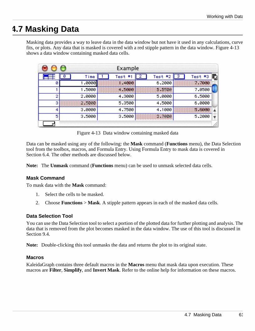
Working with Data
, curve 4-13
is. Thsed in
4.7 Masking DataMasking data provides a way to leave data in the data window but not have it used in any calculationsfits, or plots. Any data that is masked is covered with a red stipple pattern in the data window. Figureshows a data window containing masked data cells.
Figure 4-13 Data window containing masked data
Data can be masked using any of the following: the Mask command (Functions menu), the Data Selection tool from the toolbox, macros, and Formula Entry. Using Formula Entry to mask data is covered in Section 6.4. The other methods are discussed below.
Note: The Unmask command (Functions menu) can be used to unmask selected data cells.
Mask CommandTo mask data with the Mask command:
1. Select the cells to be masked.
2. Choose Functions > Mask. A stipple pattern appears in each of the masked data cells.
Data Selection ToolYou can use the Data Selection tool to select a portion of the plotted data for further plotting and analysedata that is removed from the plot becomes masked in the data window. The use of this tool is discusSection 9.4.
Note: Double-clicking this tool unmasks the data and returns the plot to its original state.
MacrosKaleidaGraph contains three default macros in the Macros menu that mask data upon execution. These macros are Filter , Simplify , and Invert Mask . Refer to the online help for information on these macros.
4.7 Masking Data 61
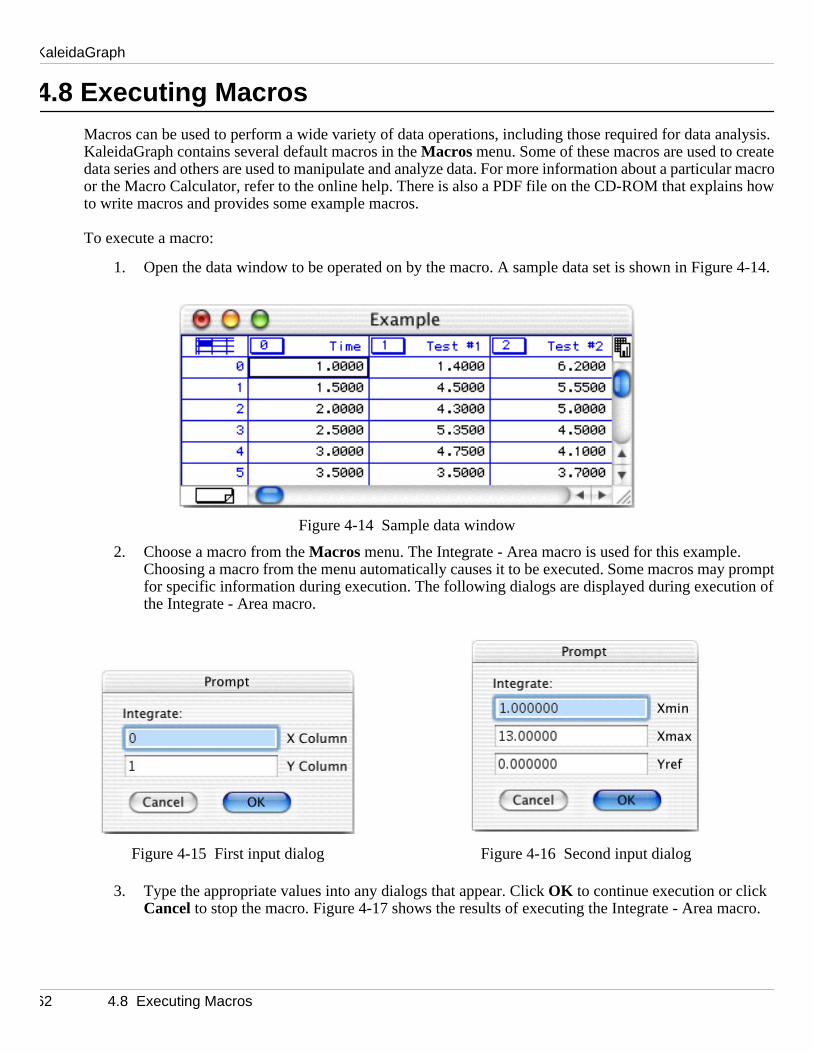
KaleidaGraph
alysis. atelar macrs how
e 4-14.
prompn o
cro.
4.8 Executing MacrosMacros can be used to perform a wide variety of data operations, including those required for data anKaleidaGraph contains several default macros in the Macros menu. Some of these macros are used to credata series and others are used to manipulate and analyze data. For more information about a particuoor the Macro Calculator, refer to the online help. There is also a PDF file on the CD-ROM that explainto write macros and provides some example macros.
To execute a macro:
1. Open the data window to be operated on by the macro. A sample data set is shown in Figur
Figure 4-14 Sample data window
2. Choose a macro from the Macros menu. The Integrate - Area macro is used for this example. Choosing a macro from the menu automatically causes it to be executed. Some macros maytfor specific information during execution. The following dialogs are displayed during executiof the Integrate - Area macro.
3. Type the appropriate values into any dialogs that appear. Click OK to continue execution or click Cancel to stop the macro. Figure 4-17 shows the results of executing the Integrate - Area ma
Figure 4-15 First input dialog Figure 4-16 Second input dialog
62 4.8 Executing Macros

Working with Data
binar
ppears,
h.
lumnsease thi
Figure 4-17 Macro results
4.9 Exporting DataKaleidaGraph provides two methods for exporting data files. You can save the data file to disk (in eitheryor text format) or you can print the data file.
4.9.1 Saving DataTo save the data to disk, choose Save Data or Save Data As from the File menu when the data window is active. If the Save Data command is used on a window that has not been saved before, a Save dialog aallowing you to specify the location and file name.
The Save Data and Save Data As commands always save the data in binary format, because this is considerably faster and more compact than text format. Binary files can only be read by KaleidaGrap
If text format is desired, choose File > Export > Tab-Delimited Text. A Save dialog appears, allowing youto specify the location and file name for the text file.
4.9.2 Printing DataTo print the data set, choose File > Print Data. The Print dialog and its options depend on the printer andoperating system.
If nothing is selected in the data window, KaleidaGraph prints the entire data set. A maximum of 15 cocan be printed on each page. Decreasing the width of the columns and scaling the output does not incrslimit.
4.9 Exporting Data 63

KaleidaGraph
64 4.9 Exporting Data
Analyzing Data
Chapter 5
lculatea, see s are
he
log
w. me
This chapter explains how to:
• View column statistics
• Place data into bins and export the results to create a Histogram, Step plot, or Spike plot.
• Perform tests to analyze single data samples.
• Perform tests to analyze two or more groups.
• Perform tests to analyze repeated measurements.
• Use a post hoc test after running a one way or one way repeated measures ANOVA.
5.1 Viewing Column StatisticsKaleidaGraph provides 12 different statistics to help analyze data. These statistics are automatically cadfor each column in the data window. If you need to calculate statistics across multiple columns of datSection 6.3 for details on using Formula Entry to do this. The equations used to calculate the statisticlisted in Section D.2.
To view statistics on a data set:
1. Select the data for which you want the statistics calculated. If you do not make a selection, tstatistics are calculated for each column in the data window.
2. Choose Functions > Statistics. The Statistics dialog, shown in Figure 5-1, is displayed. This diahas a split-screen display so that any two columns can be compared.
3. Click Copy to Clipboard if you want to paste this information into a data, plot, or layout windoYou can also select the Transposed check box so that when the data is copied, each statistic becosa column and the different variables become rows.
4. When you are finished, click OK .
5.1 Viewing Column Statistics 65

KaleidaGraph
data
Figure 5-1 Statistics dialog
5.2 Binning DataBinning data involves counting the number of data points that fall within a certain range. The binned distribution can be exported in any one of three formats for plotting or for annotating a plot.
5.2.1 Binning the DataTo bin the data:
1. Select the columns containing the variables to be binned.
2. Choose Functions > Bin Data. A dialog similar to Figure 5-2 appears.
66 5.2 Binning Data

Analyzing Data
and f bins,
ow.
Figure 5-2 Bin Data dialog
3. Bin the variables by specifying the minimum and maximum values, number of bins, Y units, where to show the counts. If you make any changes to the minimum, maximum, or number oclick Recalculate to update the count.
4. Select the appropriate Export Format for the type of plot to be created.
5. Click Copy to Clipboard.
6. Click OK .
5.2.2 Pasting the Results from the Bin Data DialogOnce the data is binned, it can be pasted into a new data window.
1. Choose File > New to create a blank data window.
2. Choose Edit > Paste. The results obtained from binning the data are placed into the data windFigure 5-3 shows binning results which were exported with a Histogram format.
5.2 Binning Data 67

KaleidaGraph
les
All dialog.
Figure 5-3 Results of binning the data
5.2.3 Creating the Plot
1. Choose the proper plot type from the Gallery menu.
• Histogram - For a single variable, choose Gallery > Bar > Column. For multiple variables, choose Gallery > Bar > Stack Column.
• Step Plot - Choose Gallery > Linear > Line.
• Spike Plot - Choose Gallery > Linear > High/Low .
2. Select the variables to be plotted.
• Histogram - Select Histogram X for the X variable and one or more binned columns for theYvariables.
• Step Plot - Select Step X for the X variable and one or more binned columns for the Y variab
• Spike Plot - Select Spike X for the X variable, plus a binned column and Zero for the Y variables.
3. Click New Plot. The following three figures show the different plot types that can be created. three were generated from the same original data set, using the same settings in the Bin DataThe only difference was the Export Format.
68 5.2 Binning Data

Analyzing Data
Figure 5-4 Histogram plot of binned data
Figure 5-5 Step plot of binned data
Figure 5-6 Spike plot of binned data
0
5
10
15
20
25
30
35
-1.5
-1.2
5 -1
-0.7
5
-0.5
-0.2
5 0
0.2
5
0.5
0.7
5 1
1.2
5
Binned Data B
0
5
10
15
20
25
30
35
-2 -1.5 -1 -0.5 0 0.5 1 1.5 2
Binned Data B
0
5
10
15
20
25
30
35
-2 -1.5 -1 -0.5 0 0.5 1 1.5
Binned Data B
5.2 Binning Data 69

KaleidaGraph
the
nt
h as
ic.
ual ral, yoted
he data.lude thdata tributed
5.3 Choosing a Statistical TestKaleidaGraph can be used to perform a variety of statistical tests. The type of test to use depends onnumber of samples and the nature of the data.
• Use a single sample test to analyze one sample to a known or hypothesized value.
• Use a group comparison test to analyze two or more different samples for statistically significadifferences.
• Use a repeated measures test to analyze the differences in two or more matched samples (sucthe same individuals before and after one or more treatments).
The table below shows the proper test to use for each experiment and the type of data collected.
5.4 Parametric and Nonparametric TestsThe statistical tests in KaleidaGraph can be divided into two categories: parametric and nonparametr
Parametric tests assume the samples are drawn from a population that is normally distributed with eqvariances. Examples of parametric tests include the t-test and analysis of variance (ANOVA). In geneushould use a parametric test if you are confident that the samples are drawn from a normally distribupopulation.
Nonparametric tests (or distribution-free tests) do not make any assumptions about the distribution of tThese tests rank the data from low to high and analyze the rank. Examples of nonparametric tests inceWilcoxon, Kruskal-Wallis, and Friedman tests. In general, you should use a nonparametric test if the represents a rank or score, or if the measurements are drawn from a population that is not normally dis
Type of Experiment
Type of Data
Numeric (normally distributed with equal variances)
Rank, score, or numeric (not normally distributed and/or
with unequal variances)
Compare one sample to a hypothetical value
One sample t-test Wilcoxon signed rank test
Compare two paired samples
Paired t-test Wilcoxon matched pairs test
Compare two unpaired samples
Unpaired t-test Wilcoxon-Mann-Whitney test
Compare three or more matched samples
One way or Two way repeated measures ANOVA
Friedman test
Compare three or more unmatched samples
One way or Two way ANOVA Kruskal-Wallis test
70 5.3 Choosing a Statistical Test

Analyzing Data
e sampl
is e.
res the
sample ver, th
is a alue isore
5.5 Analyzing One SampleKaleidaGraph provides two tests that can be used to determine whether the mean or median of a singlediffers significantly from a hypothetical value. The two tests are listed below:
• Use a single sample t-test if the sample was taken from a normally distributed population. This aparametric test that compares the mean of a single sample to a known or hypothesized valu
• Use a Wilcoxon signed rank test if the sample was taken from a non-normally distributed population or if the data consists of ranks or scores. This is a nonparametric test that compamedian of a single sample to a known or hypothesized value.
5.5.1 Entering Data for One Sample TestsThe single sample t-test and the Wilcoxon signed rank test both require that the observations for the be entered into a single data column. If the data includes a grouping variable, it can be included. Howeegrouping variable will not be used in either of these analyses.
5.5.2 Performing a Single Sample t-TestUse this test when you want to compare the mean of a sample to a known or hypothesized value.
As part of the results, KaleidaGraph calculates a t probability (P) value. This value determines if therestatistically significant difference between the mean of the sample and the hypothetical mean. If this vbelow a certain level (usually 0.05), the conclusion is that there is a difference between the two. For minformation on the results of a single sample t-test, refer to the online help.
To perform a single sample t-test:
1. Choose Functions > Student t to display a dialog similar to Figure 5-7.
5.5 Analyzing One Sample 71

KaleidaGraph
a,
ted
Figure 5-7 Student t-Test dialog
2. Click the single group button.
3. Select the column to be tested by either clicking the column name and pressing Group 1 or double-clicking the column name.
4. Enter the known or hypothesized value in the Test Value field.
5. Click Calculate. The results of the test are displayed on the right side of the dialog.
6. To export the results, click Copy Results to Clipboard. You can then paste the results into a datplot, or layout window.
7. To print the results, click the Print Results button.
8. Click OK to return to the data window.
5.5.3 Performing a Wilcoxon Signed Rank TestUse this test to compare the median of a single sample to a known or hypothesized value.
This is a nonparametric test that does not require that the samples be drawn from a normally distribupopulation. If you know that the sample is normally distributed, use a single sample t-test instead.
72 5.5 Analyzing One Sample

Analyzing Data
lly elow matio
a,
As part of the results, KaleidaGraph calculates a P value. This value determines if there is a statisticasignificant difference between the median of the sample and the hypothetical median. If this value is bacertain level (usually 0.05), the conclusion is that there is a difference between the two. For more infornon the results of a Wilcoxon signed rank test, refer to the online help.
To perform a Wilcoxon signed rank test:
1. Choose Functions > Wilcoxon to display a dialog similar to Figure 5-8.
Figure 5-8 Wilcoxon Test dialog
2. Click the single group button.
3. Select the column to be tested by either clicking the column name and pressing Group 1 or double-clicking the column name.
4. Enter the known or hypothesized value in the Test Value field.
5. Click Calculate. The results of the test are displayed on the right side of the dialog.
6. To export the results, click Copy Results to Clipboard. You can then paste the results into a datplot, or layout window.
7. To print the results, click the Print Results button.
8. Click OK to return to the data window.
5.5 Analyzing One Sample 73
KaleidaGraph
ificant and the
use on
ua
he data,
llowin
oup
orup of
scores,
pos
ne o
pariso
5.6 Analyzing Two or More GroupsKaleidaGraph provides five tests that can be used to analyze two or more different samples for a signdifference in the mean or median values. The proper test to use depends on the number of samples distribution of the data.
Comparing Two GroupsIf data was collected from two different groups of subjects (for example, male and female manatees), eof the following group comparison tests:
• Use the unpaired t-test if the samples were taken from normally distributed populations with eqlvariances. This is a parametric test that compares the sample data directly.
• Use the Wilcoxon-Mann-Whitney test if the samples were taken from non-normally distributedpopulations or if the data consists of ranks or scores. This is a nonparametric test that ranks tand analyzes the ranks instead of the raw data.
Comparing Three or More GroupsIf the samples were taken from normally distributed populations with equal variances, use one of the foggroup comparison tests:
• Use a one way ANOVA to compare the effect of a single factor on the mean of three or more grs(for example, the effect of three drugs on a group of test animals).
• Use a two way ANOVA to compare the effect of two different factors on the mean of three or megroups (for example, the effect of three drugs given at different times during the day to a grotest animals).
If the samples were taken from non-normally distributed populations or if the data consists of ranks or use the Kruskal-Wallis test.
Note: If you find a statistically significant difference using the one way ANOVA, you can use one of thethoc tests to determine which groups are different.
5.6.1 Entering Data for Group Comparison TestsThe group comparison tests in KaleidaGraph require that the data be entered in one of two ways:
• as raw data, where the data for each group is entered into a separate column.
• as indexed data, where one of the columns is a factor column or grouping variable, with the corresponding data points in one or more columns.
You can use raw data for all of the tests except the two way ANOVA. The two way ANOVA requires ortwo factor columns and one or more data columns.
Note: The groups do not have to be the same size.
The following examples show how raw and indexed data should be entered for the various group comntests.
74 5.6 Analyzing Two or More Groups
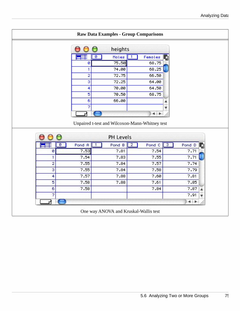
Analyzing Data
Raw Data Examples - Group Comparisons
Unpaired t-test and Wilcoxon-Mann-Whitney test
One way ANOVA and Kruskal-Wallis test
5.6 Analyzing Two or More Groups 75

KaleidaGraph
Indexed Data Examples - Group Comparisons
Unpaired t-test and Wilcoxon-Mann-Whitney test One way ANOVA and Kruskal-Wallis test
Two way ANOVA (one factor column and four columns containing the data values)
76 5.6 Analyzing Two or More Groups

Analyzing Data
mns of is in the
is a 0.05), results
tton or ust b
s. valu
a,
5.6.2 Performing an Unpaired t-TestUse this test to compare the means of two independent samples. This test can be performed on coludifferent length, since no relationship is assumed between the samples. As a special case, if Group 1assigned a Text column, it is used as a grouping variable (for example, gender) to separate the data second column into two groups.
As part of the results, KaleidaGraph calculates a t probability (P) value. This value determines if therestatistically significant difference between the two means. If this value is below a certain level (usuallythe conclusion is that there is a difference between the two group means. For more information on theof an unpaired t-test, refer to the online help.
To perform an unpaired t-test:
1. Choose Functions > Student t to display the Student t-Test dialog.
2. Click the unpaired data with equal variance or unpaired data with unequal variance button.
3. Select the columns to be tested by either clicking the column name and pressing a Group budouble-clicking the column names. If you are using a Text column as a grouping variable, it meassigned to Group 1.
4. Click the F Test check box if you want KaleidaGraph to calculate the F and F probability valueThe F probability determines if the two groups have different variances. A small F probability e(usually less than 0.05) indicates that the two groups have significantly different variances.
5. Click Calculate. The results of the test are displayed on the right side of the dialog.
6. To export the results, click Copy Results to Clipboard. You can then paste the results into a datplot, or layout window.
7. To print the results, click the Print Results button.
8. Click OK to return to the data window.
Two way ANOVA(two factor columns and one column containing the data values)
Indexed Data Examples - Group Comparisons
5.6 Analyzing Two or More Groups 77

KaleidaGraph
be specia
separat
t the compare
lly ually s of a
tton or ust b
a,
le factor.
th equare are
f a one
value. If this
ups. twee
5.6.3 Performing a Wilcoxon-Mann-Whitney TestUse this test to see if two different samples have been drawn from the same population. This test canperformed on columns of different length, since no relationship is assumed between the samples. As alcase, if Group 1 is assigned a Text column, it is used as a grouping variable (for example, gender) to ethe data in the second column into two groups.
This test assumes the samples are not normally distributed with the same variances. If you know thasamples are normally distributed, use an unpaired t-test instead. If there are more than two samples to ,use the Kruskal-Wallis test.
As part of the results, KaleidaGraph calculates a P value. This value determines if there is a statisticasignificant difference between the medians of the two groups. If this value is below a certain level (us0.05), the conclusion is that there is a difference between the two. For more information on the resultWilcoxon-Mann-Whitney test, refer to the online help.
To perform a Wilcoxon-Mann-Whitney test:
1. Choose Functions > Wilcoxon to display the Wilcoxon Test dialog.
2. Click the unpaired data button.
3. Select the columns to be tested by either clicking the column name and pressing a Group budouble-clicking the column names. If you are using a Text column as a grouping variable, it meassigned to Group 1.
4. Click Calculate. The results of the test are displayed on the right side of the dialog.
5. To export the results, click Copy Results to Clipboard. You can then paste the results into a datplot, or layout window.
6. To print the results, click the Print Results button.
7. Click OK to return to the data window.
5.6.4 Performing a One Way ANOVAUse this test when you want to see if the means of three or more different groups are affected by a singThis test is the same as the unpaired t-test, except that more than two groups can be compared.
This is a parametric test that assumes the samples are drawn from normally distributed populations wilvariances. If you know that the samples are not normally distributed, use the Kruskal-Wallis test. If theonly two samples to compare, use an unpaired t-test.
As part of the results, KaleidaGraph calculates F and P values. For more information on the results oway ANOVA, refer to the online help.
• F value - This value is the ratio of the groups mean square over the error mean square. If thisis close to 1.0, you can conclude that there are no significant differences between the groupsvalue is large, you can conclude that one or more of the samples was drawn from a differentpopulation. To determine which groups are different, use one of the post hoc tests.
• P value - This value determines if there is a statistically significant difference between the groIf this value is below a certain level (usually 0.05), the conclusion is that there is a difference benthe groups.
78 5.6 Analyzing Two or More Groups
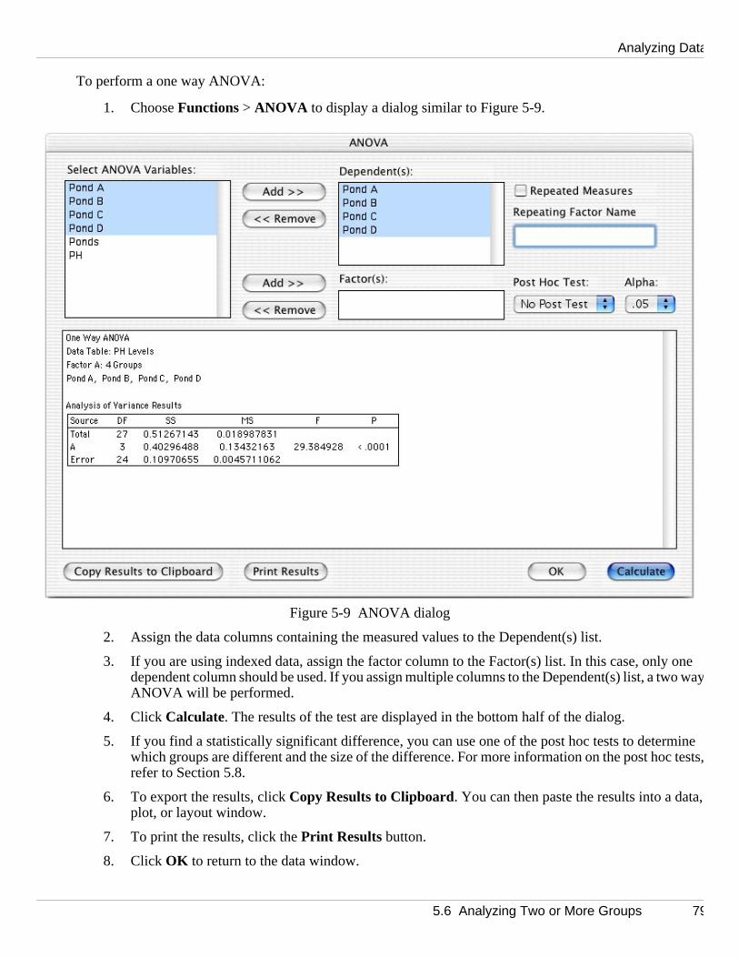
Analyzing Data
one o wa
mine tests,
a,
To perform a one way ANOVA:
1. Choose Functions > ANOVA to display a dialog similar to Figure 5-9.
Figure 5-9 ANOVA dialog
2. Assign the data columns containing the measured values to the Dependent(s) list.
3. If you are using indexed data, assign the factor column to the Factor(s) list. In this case, onlydependent column should be used. If you assign multiple columns to the Dependent(s) list, a twyANOVA will be performed.
4. Click Calculate. The results of the test are displayed in the bottom half of the dialog.
5. If you find a statistically significant difference, you can use one of the post hoc tests to deterwhich groups are different and the size of the difference. For more information on the post hocrefer to Section 5.8.
6. To export the results, click Copy Results to Clipboard. You can then paste the results into a datplot, or layout window.
7. To print the results, click the Print Results button.
8. Click OK to return to the data window.
5.6 Analyzing Two or More Groups 79

KaleidaGraph
factors.
th equaGrap
f a two
, this ction, i
en thencludferen
ups. twee
ly one
a,
ted e onl
5.6.5 Performing a Two Way ANOVAUse this test when you want to see if the means of three or more different groups are affected by twoA two way ANOVA tests three hypotheses:
• There is no difference among the levels of the first factor.
• There is no difference among the levels of the second factor.
• There is no interaction between the factors.
This is a parametric test that assumes the samples are drawn from normally distributed populations wilvariances. If you want to see the effect of only one factor on your data, use a one way ANOVA. Kaleidahdoes not have a nonparametric equivalent to the two way ANOVA.
As part of the results, KaleidaGraph calculates F and P values. For more information on the results oway ANOVA, refer to the online help.
• F value - The F value is calculated for each of the factors and the interaction. For each factorvalue is the ratio of the mean square of the factor over the error mean square. For the interatis the ratio of the interaction mean square over the error mean square.
If the F value is close to 1.0, you can conclude that there are no significant differences betwefactor levels or that there is no interaction between the factors. If this value is large, you can coethat one or more of the samples for that factor or combination of factors was drawn from a diftpopulation.
• P value - This value determines if there is a statistically significant difference between the groIf this value is below a certain level (usually 0.05), the conclusion is that there is a difference benthe groups.
To perform a two way ANOVA:
1. Choose Functions > ANOVA to display the ANOVA dialog.
2. Assign the data columns containing the measured values to the Dependent(s) list.
3. Assign one or two factor columns to the Factor(s) list. If two factor columns are assigned, ondependent column may be used.
4. Click Calculate. The results of the test are displayed in the bottom half of the dialog.
5. To export the results, click Copy Results to Clipboard. You can then paste the results into a datplot, or layout window.
6. To print the results, click the Print Results button.
7. Click OK to return to the data window.
5.6.6 Performing a Kruskal-Wallis TestUse this test when you want to see if three or more groups are affected by a single factor.
This is a nonparametric test that does not require that the samples be drawn from a normally distribupopulation. If you know that the samples are normally distributed, use the one way ANOVA. If there arytwo samples to compare, use the Wilcoxon-Mann-Whitney test.
80 5.6 Analyzing Two or More Groups

Analyzing Data
lly 0.05),f a
one
a,
As part of the results, KaleidaGraph calculates a P value. This value determines if there is a statisticasignificant difference between the medians of the groups. If this value is below a certain level (usuallythe conclusion is that there is a difference between the groups. For more information on the results oKruskal-Wallis test, refer to the online help.
To perform a Kruskal-Wallis test:
1. Choose Functions > Kruskal-Wallis to display a dialog similar to Figure 5-10.
Figure 5-10 Kruskal-Wallis dialog
2. Assign the data columns containing the measured values to the Dependent(s) list.
3. If you are using indexed data, assign the factor column to the Factor(s) list. In this case, onlydependent column may be used.
4. Click Calculate. The results of the test are displayed in the bottom half of the dialog.
5. To export the results, click Copy Results to Clipboard. You can then paste the results into a datplot, or layout window.
6. To print the results, click the Print Results button.
7. Click OK to return to the data window.
5.6 Analyzing Two or More Groups 81

KaleidaGraph
nificant and the
s befor
al
he data,
llowin
oubjects
les and
scores,
u ca
e the dat
se, onore
t tests.
5.7 Analyzing Repeated MeasurementsKaleidaGraph provides five tests that can be used to analyze two or more matched samples for a sigdifference in the mean or median values. The proper test to use depends on the number of samples distribution of the data.
Comparing Two GroupsIf data was collected from the same group of subjects (for example, the gas mileage for a number of careand after receiving a tune-up), use one of the following repeated measures tests:
• Use the paired t-test if the samples were taken from normally distributed populations with equvariances. This is a parametric test that compares the sample data directly.
• Use the Wilcoxon matched pairs test if the samples were taken from non-normally distributed populations or if the data consists of ranks or scores. This is a nonparametric test that ranks tand analyzes the ranks instead of the raw data.
Comparing Three or More GroupsIf the samples were taken from normally distributed populations with equal variances, use one of the fogrepeated measures tests:
• Use a one way repeated measures ANOVA to compare the effect of a single factor on the meanfthree or more matched groups (for example, comparing the effects of a drug on a group of sbefore, during, and after the treatment).
• Use a two way repeated measures ANOVA to compare the effect of two different factors on themean of three or more matched groups (for example, comparing the effects of a drug on mafemales before, during, and after the treatment).
If the samples were taken from non-normally distributed populations or if the data consists of ranks or use the Friedman test.
Note: If you find a statistically significant difference using the one way repeated measures ANOVA, yonuse one of the post hoc tests to determine which groups are different.
5.7.1 Entering Data for Repeated MeasurementsThe repeated measurement tests in KaleidaGraph require that the data be entered as raw data, wherafor each treatment is entered into a separate column.
The only exception is the two way repeated measures ANOVA, which requires indexed data. In this caeof the columns is a factor column or grouping variable, with the corresponding data points in two or mcolumns.
Note: Each group being analyzed must have the same number of observations.
The following examples show how the data should be entered for the various repeated measuremen
82 5.7 Analyzing Repeated Measurements

Analyzing Data
Data Examples - Repeated Measurements
Paired t-test and Wilcoxon matched pairs test
One way repeated measures ANOVA and Friedman test
5.7 Analyzing Repeated Measurements 83

KaleidaGraph
ns. This t.
is a 0.05), results
tton or
t the
a,
5.7.2 Performing a Paired t-TestUse this test to compare means on the same or related subjects over time or under different conditiotest requires columns of equal length. Any missing or extra values are skipped when running this tes
As part of the results, KaleidaGraph calculates a t probability (P) value. This value determines if therestatistically significant difference between the two means. If this value is below a certain level (usuallythe conclusion is that there is a difference between the two group means. For more information on theof a paired t-test, refer to the online help.
To perform a paired t-test:
1. Choose Functions > Student t to display the Student t-Test dialog.
2. Click the paired data button.
3. Select the columns to be tested by either clicking the column name and pressing a Group budouble-clicking the column names.
4. Click the Correlation check box if you want KaleidaGraph to calculate the correlation and correlation probability values. The correlation probability determines if there is a correlation between the two groups. A small correlation probability (usually less than 0.05) indicates thatwo groups are significantly correlated.
5. Click Calculate. The results of the test are displayed on the right side of the dialog.
6. To export the results, click Copy Results to Clipboard. You can then paste the results into a datplot, or layout window.
7. To print the results, click the Print Results button.
8. Click OK to return to the data window.
Two way repeated measures ANOVA
Data Examples - Repeated Measurements
84 5.7 Analyzing Repeated Measurements

Analyzing Data
ent runnin
t the ompare,
lly ually s of a
tton or
a,
test is
th equare only
NOV
5.7.3 Performing a Wilcoxon Matched Pairs TestUse this test to compare the median values on the same or related subjects over time or under differconditions. This test requires columns of equal length. Any missing or extra values are skipped when gthis test.
This test assumes the samples are not normally distributed with the same variances. If you know thasamples are normally distributed, use a paired t-test instead. If there are more than two samples to cuse the Friedman test.
As part of the results, KaleidaGraph calculates a P value. This value determines if there is a statisticasignificant difference between the medians of the two groups. If this value is below a certain level (us0.05), the conclusion is that there is a difference between the two. For more information on the resultWilcoxon matched pairs test, refer to the online help.
To perform a Wilcoxon matched pairs test:
1. Choose Functions > Wilcoxon to display the Wilcoxon Test dialog.
2. Click the paired data button.
3. Select the columns to be tested by either clicking the column name and pressing a Group budouble-clicking the column names.
4. Click Calculate. The results of the test are displayed on the right side of the dialog.
5. To export the results, click Copy Results to Clipboard. You can then paste the results into a datplot, or layout window.
6. To print the results, click the Print Results button.
7. Click OK to return to the data window.
5.7.4 Performing a One Way Repeated Measures ANOVAUse this test when you want to see if the same group of individuals is affected by a single factor. Thisthe same as the paired t-test, except that more than two treatments can be compared.
This is a parametric test that assumes the samples are drawn from normally distributed populations wilvariances. If you know that the samples are not normally distributed, use the Friedman test. If there atwo samples to compare, use a paired t-test.
Note: This test requires columns of equal length. If any missing or extra values are found, a one way AAis performed on the data.
5.7 Analyzing Repeated Measurements 85

KaleidaGraph
f a one
s valu ratio o
To
a
mine tests,
a,
one o ANOV
th equaeasures
As part of the results, KaleidaGraph calculates F and P values. For more information on the results oway repeated measures ANOVA, refer to the online help.
• F value - The F value is calculated for both the treatment and the subject. For the treatment, thieis the ratio of the treatment mean square over the error mean square. For the subject, it is thefthe subject mean square over the error mean square.
If this value is close to 1.0, you can conclude that there are no significant differences amongtreatments. If this value is large, you can conclude that the treatments have different effects.determine which treatments are different, use one of the post hoc tests.
• P value - This value determines if there is a statistically significant difference between the treatments. If this value is below a certain level (usually 0.05), the conclusion is that there is difference between the treatments.
To perform a one way repeated measures ANOVA:
1. Choose Functions > ANOVA to display the ANOVA dialog.
2. Assign the data columns containing the measured values to the Dependent(s) list.
3. Click the Repeated Measures check box.
4. Enter a label in the Repeating Factor Name field. This label will appear in the ANOVA results.
5. Click Calculate. The results of the test are displayed in the bottom half of the dialog.
6. If you find a statistically significant difference, you can use one of the post hoc tests to deterwhich groups are different and the size of the difference. For more information on the post hocrefer to Section 5.8.
7. To export the results, click Copy Results to Clipboard. You can then paste the results into a datplot, or layout window.
8. To print the results, click the Print Results button.
9. Click OK to return to the data window.
5.7.5 Performing a Two Way Repeated Measures ANOVAUse this test when you want to see if the same group of individuals is affected by two factors. At leastfthese factors is a repeated treatment on the same group of individuals. A two way repeated measuresAtests three hypotheses:
• There is no difference among the levels or treatments of the first factor.
• There is no difference among the levels or treatments of the second factor.
• There is no interaction between the factors.
This is a parametric test that assumes the samples are drawn from normally distributed populations wilvariances. If you want to see the effect of only one factor on your groups, use a one way repeated mANOVA. KaleidaGraph does not have a nonparametric equivalent to the two way repeated measuresANOVA.
Note: Each group must have the same number of observations for this test.
86 5.7 Analyzing Repeated Measurements
Analyzing Data
f a two
f this ents. I
square
e.
are.
a
a,
ore
ted s
e is a 0.05),f a
As part of the results, KaleidaGraph calculates F and P values. For more information on the results oway repeated measures ANOVA, refer to the online help.
• F value - The F value is calculated for each of the factors, the interaction, and the subjects. Ivalue is close to 1.0, you can conclude that there are no significant differences among treatmfthis value is large, you can conclude that the treatments have different effects.
- For the first factor, this value is the ratio of the factor mean square over the subject mean
- For the second factor, it is the ratio of the factor mean square over the error mean squar
- For the interaction, it is the ratio of the interaction mean square over the error mean squ
- For the subjects, it is the ratio of the subject mean square over the error mean square.
• P value - This value determines if there is a statistically significant difference between the treatments. If this value is below a certain level (usually 0.05), the conclusion is that there is difference between the treatments.
To perform a two way repeated measures ANOVA:
1. Choose Functions > ANOVA to display the ANOVA dialog.
2. Assign the data columns containing the measured values to the Dependent(s) list.
3. Assign a factor column to the Factor(s) list.
4. Click the Repeated Measures check box.
5. Enter a label in the Repeating Factor Name field. This label will appear in the ANOVA results.
6. Click Calculate. The results of the test are displayed in the bottom half of the dialog.
7. To export the results, click Copy Results to Clipboard. You can then paste the results into a datplot, or layout window.
8. To print the results, click the Print Results button.
9. Click OK to return to the data window.
5.7.6 Performing a Friedman TestUse this test when you want to see if a single group of individuals is affected by a series of three or mtreatments.
This is a nonparametric test that does not require that the samples be drawn from a normally distribupopulation. If you know that the samples are normally distributed, use the one way repeated measureANOVA. If there are only two samples to compare, use the Wilcoxon matched pairs test.
Note: This test requires columns of equal length.
As part of the results, KaleidaGraph calculates two different P values. These values determine if therstatistically significant difference between the groups. If the P values are below a certain level (usuallythe conclusion is that there is a difference between the groups. For more information on the results oFriedman test, refer to the online help.
5.7 Analyzing Repeated Measurements 87

KaleidaGraph
a,
To perform a Friedman test:
1. Choose Functions > Friedman to display a dialog similar to Figure 5-11.
Figure 5-11 Friedman Test dialog
2. Assign the data columns containing the measured values to the Variable(s) list.
3. Click Calculate. The results of the test are displayed in the bottom half of the dialog.
4. To export the results, click Copy Results to Clipboard. You can then paste the results into a datplot, or layout window.
5. To print the results, click the Print Results button.
6. Click OK to return to the data window.
88 5.7 Analyzing Repeated Measurements

Analyzing Data
y e whic
pairs
er
lineted
groutistic fo
there is elow a
the ys the P t ually
5.8 Choosing a Post Hoc TestOnce you have performed a one way or one way repeated measures ANOVA and found a statisticallsignificant difference, you can use one of the four post hoc tests provided by KaleidaGraph to determinhgroups are different.
• Use the Tukey HSD, Bonferroni, or Holm test to compare all possible combinations of group
• Use the Dunnett test if one column represents control data, and you want to compare all othcolumns to the control column (but not to each other).
To perform a post hoc test:
1. Verify that One Way ANOVA or One Way ANOVA – Repeated Measures is listed on the firstin the ANOVA results. The post hoc tests cannot be used with the two way or two way repeameasures ANOVA.
2. Select the desired test from the Post Hoc Test pop-up menu.
3. If necessary, select a different significance level using the Alpha pop-up menu.
4. Click Calculate. The post hoc test results will appear below the ANOVA results.
5.8.1 Tukey HSD TestThe Tukey HSD (honestly significant difference) test is a pairwise comparison of every combination ofppairs. This test calculates the mean difference for each treatment or group pair, calculates a q test stareach pair, and displays the P value that corresponds to the q test statistic. The P value determines if astatistically significant difference between the treatments or groups being compared. If this value is bcertain level (usually 0.05), the conclusion is that there is a difference between the groups.
For more information on the results of a Tukey HSD test, refer to the online help.
5.8.2 Bonferroni TestThe Bonferroni test is a pairwise comparison of every combination of group pairs. This test calculatesmean difference for each treatment or group pair, calculates a t test statistic for each pair, and displavalue that corresponds to the t test statistic. The P value determines if there is a statistically significandifference between the treatments or groups being compared. If this value is below a certain level (us0.05), the conclusion is that there is a difference between the groups.
For more information on the results of a Bonferroni test, refer to the online help.
5.8 Choosing a Post Hoc Test 89

KaleidaGraph
mean o-side
to the g for thi
ficantly ntrol anponds tocontrolat ther
5.8.3 Holm TestThe Holm test is a pairwise comparison of every combination of group pairs. This test calculates the difference for each treatment or group pair, calculates a t test statistic for each pair, and displays the twdP value that corresponds to the t test statistic.
The smallest P value is compared to the adjusted Alpha value. If the P value is greater than or equaladjusted Alpha, you can conclude that there is no significant difference for this test and any remainincomparisons. If the P value is less than the adjusted Alpha, there is a statistically significant differencestest. A new adjusted Alpha value is calculated, and the tests continue with the next smallest P value.
For more information on the results of a Holm test, refer to the online help.
5.8.4 Dunnett TestThe Dunnett test is used to determine if the mean of one group, designated as a control, differs signifrom each of the means of the other groups. This test calculates the mean difference between the codeach treatment or group, calculates a q test statistic for each pair, and displays the P value that corresthe q test statistic. The P value determines if there is a statistically significant difference between the and the group being compared. If this value is below a certain level (usually 0.05), the conclusion is theis a difference between the groups.
For more information on the results of a Dunnett test, refer to the online help.
90 5.8 Choosing a Post Hoc Test

Working with Formula Entry
Chapter 6
widrtain
In cess o
The Formula Entry window is a very powerful tool for data analysis. Using this window, you can apply aerange of algebraic functions to your data. It also provides a formula script feature to help automate cefunctions in the program.
This chapter explains how to:
• Enter and execute formulas.
• Reference columns, cells, and memory locations in a formula.
• Create multi-line formulas.
• Calculate statistics.
• Linearly interpolate data.
• Obtain values from a curve fit.
• Create shorthand references for constants, variables, and functions in the library.
• Automate the process of creating plots using formula scripts.
6.1 Formula Entry BasicsThis section provides the basic information you need to start working with the Formula Entry window.addition to this section, you may also want to refer to Section 2.5.2, which guides you through the profexecuting several formulas.
6.1 Formula Entry Basics 91

KaleidaGraph
tothe
hese
r more
our
.
u have mands
6.1.1 Formula Entry WindowChoose Windows > Formula Entry to display the window in Figure 6-1. Use the Formula Entry windowenter formulas that generate and manipulate data in the active data window. The various features of Formula Entry window are discussed below.
Figure 6-1 Formula Entry window
1. Formula Entry Menu BarThese menus contain all of the functions that are available in Formula Entry. The commands in tmenus are described in Section 6.9.
2. Text FieldFormulas are entered in this area of the window.
3. Posted NoteThis is an internal text editor where multiple functions can be strung together. See Section 6.2 foinformation on multi-line formulas.
4. Function ButtonsUsing these buttons, you can assign frequently used formulas to the first eight function keys of ykeyboard. This topic is discussed in Section 6.1.6.
5. Degrees/Radians ButtonsThese buttons determine whether the results of trigonometric functions are in degrees or radians
6. Help...Click this button to display the Help dialog.
7. RunThis button is used to execute the current formula. Formulas can also be executed by typing Enter (Windows) or Return (Macintosh). If a data window is not open, this button is unavailable.
6.1.2 Formula Entry MenusThe menus in Formula Entry contain all of the commands and operators that are available for use. Yothe option of choosing the commands from the menu or typing them into the window. Each of the comis discussed in detail in Section 6.9.
3 7
62
1 5
4
92 6.1 Formula Entry Basics
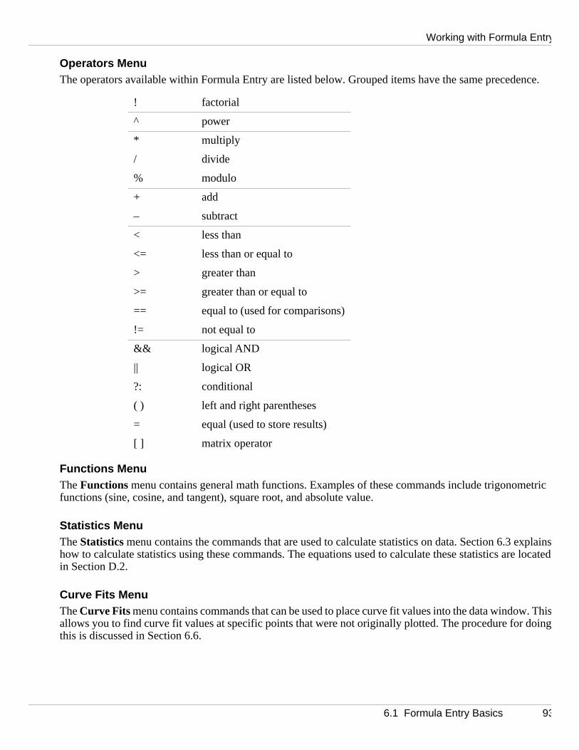
Working with Formula Entry
ence.
etric
xplainse located
w. Thidoing
Operators MenuThe operators available within Formula Entry are listed below. Grouped items have the same preced
Functions MenuThe Functions menu contains general math functions. Examples of these commands include trigonomfunctions (sine, cosine, and tangent), square root, and absolute value.
Statistics MenuThe Statistics menu contains the commands that are used to calculate statistics on data. Section 6.3 ehow to calculate statistics using these commands. The equations used to calculate these statistics arin Section D.2.
Curve Fits MenuThe Curve Fits menu contains commands that can be used to place curve fit values into the data windosallows you to find curve fit values at specific points that were not originally plotted. The procedure for this is discussed in Section 6.6.
! factorial
^ power
* multiply
/ divide
% modulo
+ add
– subtract
< less than
<= less than or equal to
> greater than
>= greater than or equal to
== equal to (used for comparisons)
!= not equal to
&& logical AND
|| logical OR
?: conditional
( ) left and right parentheses
= equal (used to store results)
[ ] matrix operator
6.1 Formula Entry Basics 93

KaleidaGraph
their
is
uch as
cations the lef
is not ult in
oany dattion
d in a d cells
ow.
ded in a
Special MenuThe Special menu contains commands that use either a Boolean expression or a text string as part ofdefinition.
Library MenuThe Library menu displays all of the definitions in the current library. If the library is empty, this menualso empty. For more information on the library, see Section 6.8.
6.1.3 Formula StructureA formula calculates new values from existing data in the data window. A formula can be a simple mathematical operation, such as multiplying a column by a constant, or a more complex operation, scalculating the root mean square of a specific group of data.
Formulas are created using a combination of column references, operators, and functions. Memory loand constants can also be used in a formula. Formulas are usually constructed with the destination totof the equal sign (=) and the calculation to the right of the equal sign. One exception is the name function, which specifies the output column as one of the parameters.
The results of a formula can be stored in another column, a cell, or a memory register. If a destinationspecified, the results are displayed in a dialog similar to Figure 6-2. This is useful for formulas that resasingle value, such as the commands located in the Statistics menu.
Figure 6-2 Result dialog
6.1.4 Referencing Columns, Cells, and Memory RegistersColumn numbers range from 0 to 999 and need to be preceded by a c when used in a formula (c0, c1, and son). Column numbers are displayed in a box at the top of the column and are referenced to the start of aselection. Please note that when a selection is made in the data window, the first column in the selecbecomes column 0.
Calculations involving columns are performed on a row-by-row basis. If two or more columns are usecalculation, corresponding cells in the same row are used to determine the results. If empty or maskeare encountered during the calculation, the corresponding cell in the destination column is empty.
Individual cells can be referenced in a formula using the cell function. The syntax of this function is cell(row#, col#). Using this function, it is possible to store and retrieve data anywhere in the data wind
Memory registers range from 0 to 99 and need to be preceded by an m when used in a formula (m0, m1, anso on). Memory registers are useful in calculations that result in a single value. The value can be stormemory register and used at a later time in other calculations.
94 6.1 Formula Entry Basics

Working with Formula Entry
try ct on
ote ca
he data t be
signelas in
yo
Some example formulas are shown below:
6.1.5 Entering and Executing a FormulaThis section provides the general instructions for entering and executing a formula in the Formula Enwindow. Section 2.5.2 provides a detailed example of running several formulas and viewing their effethe data window.
To enter and execute a formula:
1. Open the data window to be operated on by the formula.
2. Choose Windows > Formula Entry .
3. Enter the formula into the text field of Formula Entry. You can either type the operators and functions or choose them from the appropriate menus in the Formula Entry window.
4. Multiple formulas can be entered by separating each formula with a semicolon. The Posted Nnalso be used to enter multiple formulas. This topic is covered in Section 6.2.
5. Click Run to execute the formula.
Note: The results of a formula are based on the data at the time the formula is executed. Changing tdoes not cause the results to automatically recalculate. To update the results, the formula musexecuted again.
6.1.6 Assigning Formulas to Function ButtonsYou can store formulas in any of the eight function buttons in Formula Entry. Any formulas that are asdto these buttons are saved in the Macros file. It is recommended that you store frequently-used formuF2–F8 and leave F1 for entering general formulas that do not need to be saved.
To assign a formula to a particular function button:
1. Select the appropriate function button in Formula Entry using one of the following methods:
• Click the button in the Formula Entry window.
• Press the corresponding function key on the keyboard.
• Hold down Ctrl (Windows) or (Macintosh) and press the number of the function button uwant to select.
2. Enter the formula into the text field of Formula Entry.
Example Formulas
c1 = c0/1000 cell(0,5) = cell(0,0) – 11
c5 = (c1+c2) * (c3–c4) m1 = npts(c0)
cell(0,2) = mean(c1) m10 = cell(0,0)
6.1 Formula Entry Basics 95

KaleidaGraph
xecuted ion es a
red i
6.2 Multi-Line FormulasWith the use of the Posted Note in Formula Entry, you can string formulas together and have them esequentially. Each formula should be entered on a separate line and end with a semicolon. This sectprovides the general instructions for entering and executing a multi-line formula. Section 2.5.2 providdetailed example of executing a multi-line formula and viewing its effect on the data window.
To enter and execute a multi-line formula:
1. Open the data window to be operated on by the formula.
2. Choose Windows > Formula Entry .
3. Click the Posted Note button ( ) to display the text editor.
4. Enter the individual formulas into the Posted Note. Figure 6-3 shows a multi-line formula ententhe text editor. Notice that each formula is entered on a separate line and is terminated by a semicolon.
Figure 6-3 Posted Note with formula entered
5. When you are finished entering the formulas, choose File > Close to leave the editor. The FormulaEntry window appears, displaying the message shown in Figure 6-4.
Figure 6-4 Formula Entry after exiting the Posted Note
6. Click Run to execute the formulas in the Posted Note.
96 6.2 Multi-Line Formulas

Working with Formula Entry
able by
e m the
sing
e stics ar
ction. cell, odual
6.2.1 Adding CommentsComments can be added to a multi-line formula. Comments are used to make the formula more readdescribing the purpose of the program and the use of each individual formula.
Comments can be added anywhere in the Posted Note with the use of a semicolon. Anything after thsemicolon to the first occurrence of a carriage return is treated as a comment. The following lines fromulti-line formula in Figure 6-3 have had comments added.
c0 = (–0.5 + ran()) * 10; Fill c0 with random numbers between –5 and 5.macro("Invert Mask"); Execute the Invert Mask macro from the Macros menu.name("Values", c0); Change the title of c0 to "Values."
6.2.2 Saving Multi-Line FormulasMulti-line formulas can be saved as a text file by choosing File > Save As in the Posted Note window. Thistext file can be reopened at a later time by clicking the Posted Note button in Formula Entry and chooFile > Open.
6.3 Calculating Statistics with Formula EntryKaleidaGraph provides 12 commands in the Statistics menu to help you analyze data. The statistics can bcalculated on individual columns or a specific range of data. The equations used to calculate the statielisted in Section D.2.
6.3.1 Individual Column StatisticsStatistics are calculated on individual columns by entering the column number within the statistics funThis function results in a single data value, which can be displayed in a dialog or stored in a column, rmemory register. The following table shows some example formulas that calculate statistics on indivicolumns.
Formula Result
mean(c12) Finds the mean of column 12 and displays the result in a dialog.
c4 = stderr(c3) Determines the standard error for column 3 and places the result in column 4.
cell(0,5) = std(c15) Finds the standard deviation of column 15 and stores the result in row 0 of column 5.
m2 = cmin(c11) Determines the minimum value in column 11 and stores the result in memory register 2.
6.3 Calculating Statistics with Formula Entry 97
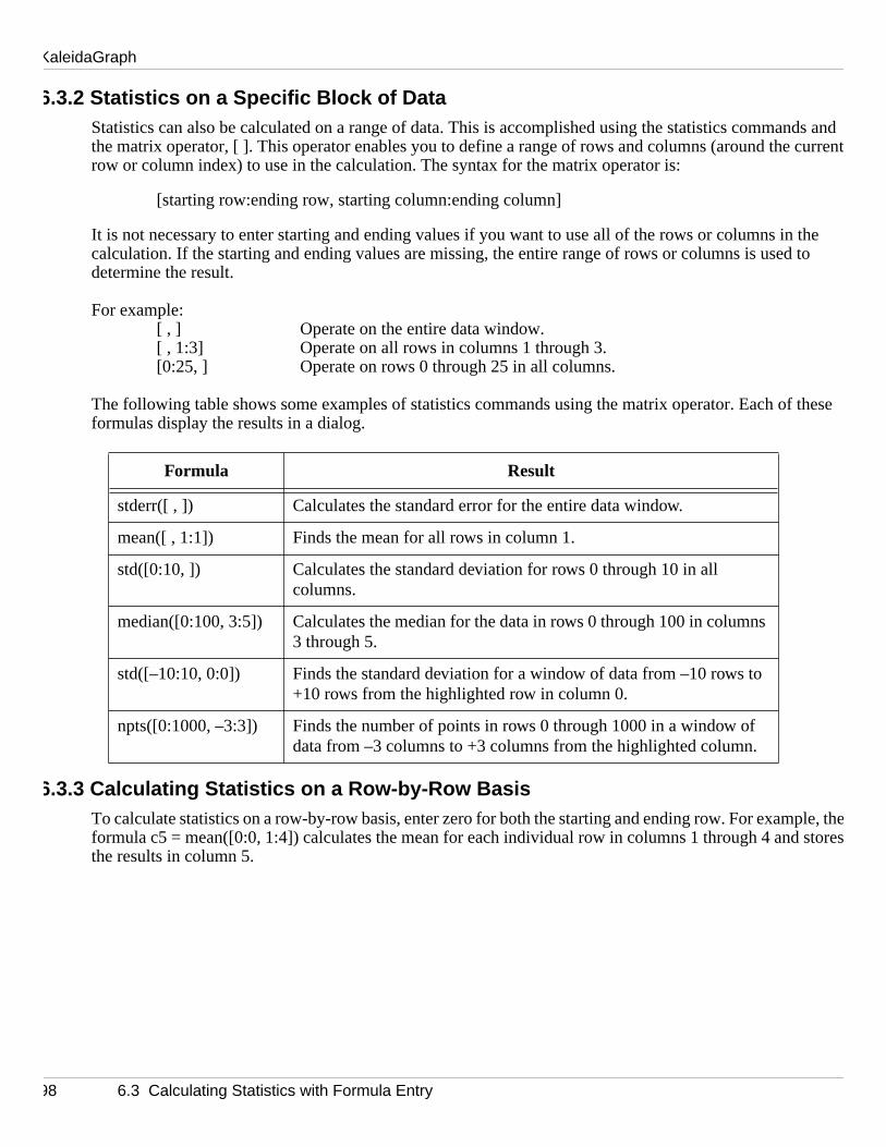
KaleidaGraph
nds and curren
the to
these
ple, th stores
6.3.2 Statistics on a Specific Block of DataStatistics can also be calculated on a range of data. This is accomplished using the statistics commathe matrix operator, [ ]. This operator enables you to define a range of rows and columns (around thetrow or column index) to use in the calculation. The syntax for the matrix operator is:
[starting row:ending row, starting column:ending column]
It is not necessary to enter starting and ending values if you want to use all of the rows or columns incalculation. If the starting and ending values are missing, the entire range of rows or columns is useddetermine the result.
For example:[ , ] Operate on the entire data window.[ , 1:3] Operate on all rows in columns 1 through 3.[0:25, ] Operate on rows 0 through 25 in all columns.
The following table shows some examples of statistics commands using the matrix operator. Each offormulas display the results in a dialog.
6.3.3 Calculating Statistics on a Row-by-Row BasisTo calculate statistics on a row-by-row basis, enter zero for both the starting and ending row. For exameformula c5 = mean([0:0, 1:4]) calculates the mean for each individual row in columns 1 through 4 andthe results in column 5.
Formula Result
stderr([ , ]) Calculates the standard error for the entire data window.
mean([ , 1:1]) Finds the mean for all rows in column 1.
std([0:10, ]) Calculates the standard deviation for rows 0 through 10 in all columns.
median([0:100, 3:5]) Calculates the median for the data in rows 0 through 100 in columns 3 through 5.
std([–10:10, 0:0]) Finds the standard deviation for a window of data from –10 rows to +10 rows from the highlighted row in column 0.
npts([0:1000, –3:3]) Finds the number of points in rows 0 through 1000 in a window of data from –3 columns to +3 columns from the highlighted column.
98 6.3 Calculating Statistics with Formula Entry

Working with Formula Entry
n 6.9.
ns. The
olum in
6.4 Masking Data with Formula EntryKaleidaGraph supports two functions (mask and filter ) that can be used to mask data via a formula. An unmask function is also provided to return the data to normal. These commands are defined in SectioSome example uses of these commands are listed below.
Note: For more information on masking and unmasking data, refer to Section 4.7.
6.5 Interpolating DataKaleidaGraph is able to perform linear interpolation through the use of the table function in Formula Entry. The table command performs a linear approximation of a number (x) based on the data in two columsyntax for this command is table(x, x col#, y col#), such that for a given x value, this function returns an estimate for y.
Figure 6-5 shows an example use of the table function. The first two columns contain X-Y data points. Cn2 contains a new set of X values for which you want to find the corresponding Y values. The Y valuescolumn 3 were found by executing the formula c3=table(c2, c0, c1) in Formula Entry.
Figure 6-5 Sample data window
Formula Result
mask(c0 < 0, c0) Masks any negative values in c0.
mask(c1 < c2, c2) Masks any cells in c2 whose value is greater than the corresponding cell in c1.
filter(–1, 1, c0) Masks all cells in c0 that are less than –1 or greater than 1.
unmask(c0 > 0, c3) Unmasks any cells in c3 if the corresponding value in c0 is positive.
6.4 Masking Data with Formula Entry 99

KaleidaGraph
ong a te the
a.
rmulata
a ploe.
point
ccurat the
data
6.6 Obtaining Values from a Curve FitThe Curve Fits menu in Formula Entry contains commands that can be used to analyze the values alfitted curve. These commands enable you to find values at any point on the curve, as well as calcularesidual error between the fitted curve and the original data.
Before you can get values from a curve fit, you must first create a plot and apply a curve fit to the datOtherwise, an error message is displayed when you try to run the formula.
Note: It is possible to get the curve fit values and residual values into the data window without using FoaEntry. See Section 10.6.3 for more information on exporting the results of a curve fit into the dwindow.
The following sections show how to get values from a curve fit into the data window. Figure 6-6 showstwith a Polynomial curve fit applied (represented by the dashed line) which will be used as an exampl
Figure 6-6 Sample plot with Polynomial fit applied
6.6.1 Getting Curve Fit Values into the Data WindowThe following steps explain how to use Formula Entry to obtain values from the curve fit at specific Xlocations. The X positions can be the original column of X values, a new column of values, or a singlealong the X axis.
Note: Unless the curve fit is extrapolated to the axis limits (see Section 10.8.1), the results are only aeif the X values lie within the original range of the data. If the values fall outside the data range,results are linearly interpolated.
To calculate values from a curve fit:
1. Activate the data window that contains the fitted variables. Figure 6-7 shows a portion of theused to create the sample plot.
-0.2
0
0.2
0.4
0.6
0.8
1
-1.5 -1 -0.5 0 0.5 1 1.5
Sinc(5x)
Y = M0 + M1*x + ... M8*x8 + M9*x9
0.74336M0
-2.2635e-06M1
-1.5172M2
5.393e-06M3
0.57377M4
-2.3555e-06M5
0.89315R
100 6.6 Obtaining Values from a Curve Fit
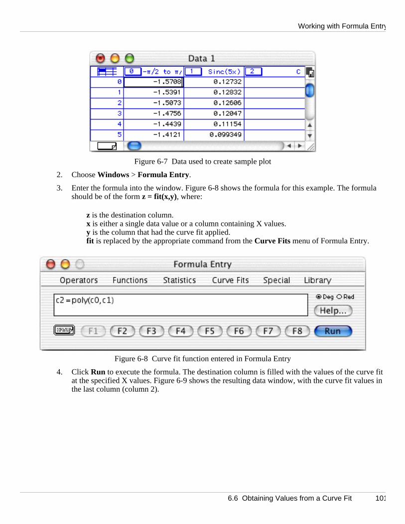
Working with Formula Entry
la
fit es in
Figure 6-7 Data used to create sample plot
2. Choose Windows > Formula Entry .
3. Enter the formula into the window. Figure 6-8 shows the formula for this example. The formushould be of the form z = fit(x,y), where:
z is the destination column.x is either a single data value or a column containing X values.y is the column that had the curve fit applied.fit is replaced by the appropriate command from the Curve Fits menu of Formula Entry.
Figure 6-8 Curve fit function entered in Formula Entry
4. Click Run to execute the formula. The destination column is filled with the values of the curveat the specified X values. Figure 6-9 shows the resulting data window, with the curve fit valuthe last column (column 2).
6.6 Obtaining Values from a Curve Fit 101

KaleidaGraph
ant to
ers e curv
ow to
a wit
m a
Figure 6-9 Data window containing curve fit values
Note: This method uses the curve fit points originally calculated when the fit was applied. You may wincrease the number of calculated points to make the values from the fit more accurate. See Section 10.8.3 for instructions on increasing the number of curve fit points.
6.6.2 Using the Calculated Equation to Find ValuesThe most accurate method of getting values from a fit is to use the original equation and the parametcalculated by KaleidaGraph. This is not possible when a Smooth, Weighted, Cubic Spline, or Interpolatefit is applied to the data, because these curve fits do not result in an equation.
To calculate values using the curve fit’s equation:
1. Copy the curve fit coefficients to the Calculator. Refer to Section 10.6.3 if you are unsure of hdo this. If you applied a General curve fit, you can skip this step because the parameters areautomatically stored in the Calculator.
2. Activate the data window that contains the fitted variables. Figure 6-10 shows the original datha column containing new X values (column 2).
Figure 6-10 Data window containing new X values
3. Choose Windows > Formula Entry .
4. Enter your formula into the window. Figure 6-11 shows the formula used to obtain values frocurve fit at designated points, where:
102 6.6 Obtaining Values from a Curve Fit

Working with Formula Entry
fit es in
. Yo
d as this allows easiest n
cause
c3 is the destination column for the curve fit values.c2 is the column containing the new X values.m0–m5 are the curve fit coefficients previously copied to the Calculator.
Figure 6-11 Using the curve fit equation to calculate values
5. Click Run to execute the formula. The destination column is filled with the values of the curveat the specified X values. Figure 6-12 shows the resulting data window, with the curve fit valuthe last column (column 3).
Figure 6-12 Data window containing curve fit values
Note: This method can similarly be used to calculate the X value when the Y value on the fit is knownuneed to rearrange the formula so that it solves for X instead of Y.
6.7 Performing Date and Time CalculationsIt is possible to perform calculations on columns containing dates and times. Internally, dates are storeetotal number of seconds since Jan. 1, 1904 and times are stored as a relative number of seconds. Thyou to perform calculations on date and time data just as you would with any other kind of data. The way to illustrate this is to use the Column Format command (Data menu) to change the format of a columcontaining dates or times to the Double format. The column now shows the total number of seconds.
Note: You do not have to change the format of the column before using it in a calculation. This is beKaleidaGraph automatically stores the values as a total number of seconds.
6.7 Performing Date and Time Calculations 103
KaleidaGraph
se in d
, ope
, matrticula
riableser limi
curv. Pleastheses
itionse emicolo fit
If you
isk.
ary toes
6.8 Using the LibraryKaleidaGraph provides a library which can be used to define constants, variables, and functions for uFormula Entry, the Function plot, and the General curve fit. Using the library, you can create shorthanreferences to values and functions that you use on a regular basis.
6.8.1 Library BasicsThe library is displayed by choosing either Macros > Library or Curve Fits > General > Library . The current library is displayed in a text editor. Once you are in the editor, you can modify the current libraryna saved library, or create a new library.
The default library provided with KaleidaGraph contains a number of definitions for variables, constantshfunctions, and curve fit equations. The definitions are grouped together to make it easier to locate a parfunction, but this is not a requirement. You can place the definitions in any order you choose.
One of the main reasons for using the library is to form aliases or shorthand references for functions, va,and constants. This is particularly useful for defining sections of a formula that exceed the 256 characttin the Formula Entry, Function plot, and General curve fit windows.
6.8.2 Creating Library DefinitionsAny of the definitions in the library can be called from Formula Entry, the Function plot, or the General efit. KaleidaGraph searches the current library for any substitutions and makes them before proceedingenote that KaleidaGraph substitutes the definition, so you may want to enclose the definition with parento maintain the proper syntax after the substitution takes place.
Use the same syntax shown in the default library to create your own definitions. All of the library definare terminated with a semicolon. Anything following the semicolon is treated as a comment, unless thsemicolon is preceded by a backslash (\). The purpose of the backslash is to treat the data after the snas a continuation of the function. This is normally used to set up initial conditions when defining curveequations.
When creating your shorthand references, it is important to note that the library is not case sensitive.had two functions named S1() and s1(), either one could be substituted by KaleidaGraph.
6.8.3 Creating a Custom LibraryThe library is saved as part of the Macros file. To create a custom library, choose Macros > Library and savethe default library to disk (using the Save As command in the editor). Then, choose File > New to start a newlibrary. Use the same syntax shown for the default library. When completed, save the new library to d
KaleidaGraph references whichever library is currently open. To reference a new library, use the Open command in the editor to locate and load the library you want to use. If you want to tie a particular libra macros file, use the File > Export > Macros command to save the macros file. The current library becomthe default library for that particular macros file.
104 6.8 Using the Library

Working with Formula Entry
amples
culation.
6.9 Function Descriptions and SyntaxThis section describes each of the operators and functions available in the Formula Entry menus. Exare provided for each of the items.
6.9.1 Operators Menu
( ) - The parentheses are used with almost every formula to enclose the variable being used in the calThey are also used to set the priority order for calculations.
Example: c3 = (cos(c2) * sin(c1)) + ((2 * tan(c0)) / sqrt(pi))
^ - This operator raises the preceding value to the specified power.
Examples: 5^2, c3 = c1^(1/c0)
* - This operator multiplies two values together.
Examples: 23 * m0, c3 = .9087 * c5
/ - This operator is used for division.
Examples: c4 = c0 / 12.234, c12 = (c8 + c5) / c2
+ - This operator is used for addition.
Examples: c3 = (c2 + c1 + c0) / 3, c12 = 198 + c10
– - This operator is used for subtraction.
Examples: c9 = c8 – c6, c19 = (c12 – c3) / c5
% - This operator performs the mod function.
Examples: c9 = c8 % 4, c13 = c12 % c3
! - This operator calculates the factorial of a number.
Examples: 7!, c13 = c10!
< - This operator compares two values to see if one is less than the other.
Examples: mask(c1 < 3, c1), unmask(c2 < –12, c3)
<= - This operator compares two values to see if one is less than or equal to the other.
Examples: mask(c4 <= c5, c6), unmask(c2 <= 23, c12)
> - This operator compares two values to see if one is greater than the other.
Examples: mask(c1>1, c0), unmask(c4 > c3), c5)
>= - This operator compares two values to see if one is greater than or equal to the other.
Examples: mask(c12 >= 12.34, c12), unmask(c11 >= –5, c11)
6.9 Function Descriptions and Syntax 105

KaleidaGraph
ust
tru
d in on
x of th
tion. If he resul
g in the
== - This operator compares two values to see if they are equal to each other.
Examples: mask(c1 == 4, c1), unmask(c3 == c2, c1)
!= - This operator compares two values to see if they are unequal.
Examples: mask(c2 != c4, c2), unmask(c3 != 2, c3)
&& - This operator performs a logical and on two Boolean expressions. The result of both expressions mbe true (non-zero) for the logical and to be true.
Examples: c3 = (c0>1 && c0<15) ? c0 : 0.5, c1 = (c2>3 && c2<11) ? c2 : 0
|| - This operator performs a logical or on two Boolean expressions. The result of one expression must bee(non-zero) for the logical or to be true.
Examples: c1 = (c2>1 || c3>1) ? c1 : c4, c2 = (c1<0 || c1 == 0.5) ? 0 : c1
?: - This operator performs a conditional test on a Boolean expression. This operator can be expresseeof two ways:
• if (Boolean) expression 1 else expression 2
• (Boolean) ? expression 1 : expression 2
If the result of the Boolean is true (non-zero), return expression 1; if it is false, return expression 2.
Examples: c9 = (c2>.5 || c3>.1) ? c11 : c4, c1 = (c2>1 && c2<10) ? c2 : 0.1
= - This operator is used to place the result of a calculation into a column, cell, or memory location.
Examples: m0 = 12 * m1, c1 = sqrt(c0), c2 = cos(c0), cell(0,5) = cmin(c0)
[ ] - The matrix operator is used to specify a range of data for use in a statistical calculation. The syntaeoperator is: [starting row:ending row, starting column:ending column].
It is not necessary to enter starting and ending values to use all of the rows or columns in the calculathe starting and ending values are missing, the entire range of rows or columns is used to determine tt
Examples: cmax([ 0:23, 3:10]), c18 = median([ , 12:14])
6.9.2 Functions Menu
abs(x) - Determines the absolute value of a number.
Examples: abs(–5), abs(m3), c3 = abs(c2)
cell(row#, col#) - Gets or sets the value of a specific cell.
Example: cell(0, 2) = 5.5 * cell(1, 3), cell(10, 13) = sqrt(cell(15, 11))
cos(x) - Determines the cosine of a number. The number is in radians or degrees, based on the settinFormula Entry window.
Examples: cos(30), cos(m8), c4 = cos(c2)
diff(x) - Calculates the difference between each value and the one that follows it.
Examples: c5 = diff(c2), c11 = diff(c10)
106 6.9 Function Descriptions and Syntax

Working with Formula Entry
0,
g
n the
e settin
on the
erf(x) - Calculates the error function of a value. This function has the following limiting values: erf(0) =erf(∞) = 1, and erf(–x) = –erf(x).
Examples: erf(2), c10 = erf(c9)
erfc(x) - Calculates the complementary error function of a value. This function has the following limitinvalues: erfc(0) = 1, erfc(∞) = 0, and erfc(–x) = 2–erfc(x).
Examples: erfc(.5), c20 = erfc(c19)
exp(x) - Calculates the value of e (2.7182...) raised to a power.
Examples: exp(3), exp(m1), c10 = exp(c2)
fract(x) - Returns the fractional portion of a number.
Examples: fract(2.83), c12 = fract(c9)
index() - Returns the current row number (starting at 0).
Example: c5 = index() * .5, c11 = index() – 64
inorm(x) - Determines the inverse of the normal distribution for a number between zero and 100%.
Examples: inorm(25), inorm(m2), c10 = inorm(c9)
int(x) - Returns the integer portion of a number.
Examples: int(2.83), c12 = int(c9)
invcos(x) - Determines the inverse cosine of a number. The number is in radians or degrees, based osetting in the Formula Entry window.
Examples: invcos(.5), invcos(m3), c6 = invcos(c5)
invsin(x) - Determines the inverse sine of a number. The number is in radians or degrees, based on thgin the Formula Entry window.
Examples: invsin(.219), invsin(m0), c15 = invsin(c10)
invtan(x) - Determines the inverse tangent of a number. The number is in radians or degrees, based setting in the Formula Entry window.
Examples: invtan(1), invtan(m2), c9 = invtan(c8)
ln(x) - Calculates the natural logarithm (base e) of a number.
Examples: ln(8), ln(m5), c12 = ln(c9)
log(x) - Calculates the common logarithm (base 10) of a number.
Examples: log(20), log(m10), c18 = log(c15)
norm(x) - Determines the normal distribution of a number between zero and 100%.
Examples: norm(23), norm(m5), c7 = norm(c5)
6.9 Function Descriptions and Syntax 107
KaleidaGraph
n the
n the of the
ng in the
pi - Represents the value of π (3.1415926...).
Example: c10 = pi * c9, c11 = 3 * pi * c9
ran() - Generates a random number between zero and one.
Examples: c15 = ran(), c9 = c8 * ran()
rsum(col#) - Computes the running sum of a column.
Example: c3 = rsum(c2), c10 = rsum(c9)
sin(x) - Determines the sine of a number. The number is in radians or degrees, based on the setting iFormula Entry window.
Examples: sin(45), sin(m6), c11 = sin(c10)
sqrt(x) - Calculates the square root of a number.
Examples: sqrt(192), sqrt(m9), c6 = sqrt(c5)
table(x, x col#, y col#) - The table command performs a linear approximation of a number (x) based odata in two columns. The result is that for a given x, this function returns an estimate for y. The ordercolumns determines what value is returned. This function has the following constraints:
• You cannot have masked or empty cells in either the x col# or y col#.
• y col# = f(x col#) may only describe a single value function.
• It does not operate on a subset of rows within a column.
Examples: table(2.5, c0, c1), c4 = table(c3, c0, c1)
tan(x) - Determines the tangent of a number. The number is in radians or degrees, based on the settiFormula Entry window.
Examples: tan(68), tan(m10), c5 = tan(c4)
6.9.3 Statistics Menu
cmin(x) - Determines the minimum value within the specified data.
Examples: cmin(c5), cmin([ , 0:10]), c2 = cmin([ , ])
cmax(x) - Determines the maximum value within the specified data.
Examples: cmax(c15), cmax([ 0:23, 3:10]), c13 = cmax([ , 0:12])
csum(x) - Calculates the sum of the data values.
Examples: csum(c9), csum([ , 0:3]), c12 = csum([0:50, 3:8])
kurtosis(x) - Calculates the kurtosis of the specified data.
Examples: kurtosis(c12), kurtosis([0:5, ]), c5 = kurtosis([0:25, 0:1])
mean(x) - Calculates the mean of the data.
Examples: mean(c0), mean([ , 2:3]), c11 = mean([ , ])
108 6.9 Function Descriptions and Syntax
Working with Formula Entry
d, thiolum
s the
mine
median(x) - Calculates the median of the data range.
Examples: median(c3), median([2:10, 0:1]), c17 = median([ , 12:14])
npts(x) - Determines the number of points within the specified data range.
Examples: npts(c1), npts([ , 0:5]), c10 = npts([ , ])
rms(x) - Calculates the RMS (root mean square) of the data range.
Examples: rms(c3), rms([ , 1:1]), c5 = rms([12:21, ])
skew(x) - Calculates the skewness of the data range.
Examples: skew(c15), skew([ , 3:10]), c13 = skew([–10:10, 2:2])
std(x) - Calculates the standard deviation of the data range.
Examples: std(c10), std([12:120, ]), c3 = std([ , ])
stderr(x) - Calculates the standard error of the data.
Examples: stderr(c4), stderr([–5:5, 15:19]), c3 = stderr([ , ])
var(x) - Calculates the variance of the specified data range.
Examples: var(c6), var([0:25, ]), c3 = var([ , ])
6.9.4 Curve Fits Menu
expr(x, col#) - Given an x value and a column that has an Exponential curve fit applied, this function determines the value from the fit at the x point.
Examples: expr(105, c10), c11 = expr(c8,c9)
gen(" ", x, col#) - Given the name of a General curve fit, an x value, and a column that has the fit appliesfunction determines the value at the x point. If no name is given, the first General fit that is found in the cnis used.
Examples: gen("fit1", 22, c1), c5 = gen(c0, c1), c11 = ("gaussian", c8, c9)
interp(x, col#) - Given an x value and a column that has an Interpolate curve fit applied, this function determines the value from the fit at the x point.
Examples: interp(11.95, c2), c19 = interp(c15, c18)
lin(x, col#) - Given an x value and a column that has a Linear curve fit applied, this function determinevalue from the fit at the x point.
Examples: lin(–12.5, c1), c10 = lin(c9, c5)
logr(x, col#) - Given an x value and a column that has a Logarithmic curve fit applied, this function detersthe value from the fit at the x point.
Examples: logr(1300, c8), c12 = logr(c3, c4)
6.9 Function Descriptions and Syntax 109

KaleidaGraph
mine
es th
mine
mines
s it. ndow.
t")
ent
.
, this
poly(x, col#) - Given an x value and a column that has a Polynomial curve fit applied, this function detersthe value from the fit at the x point.
Examples: poly(.0034, c15), c14 = poly(c12, c1)
pow(x, col#) - Given an x value and a column that has a Power curve fit applied, this function determinevalue from the fit at the x point.
Examples: pow(119, c10), c3 = pow(c0, c2)
smooth(x, col#) - Given an x value and a column that has a Smooth curve fit applied, this function detersthe value from the fit at the x point.
Examples: smooth(11.15, c2), c4 = smooth(c2, c3)
spline(x, col#) - Given an x value and a column that has a Cubic Spline curve fit applied, this functiondetermines the value from the fit at the x point.
Examples: spline(–23.098, c17), c4 = spline(c3, c8)
wgt(x, col#) - Given an x value and a column that has a Weighted curve fit applied, this function deterthe value from the fit at the x point.
Examples: wgt(15.657, c2), c9 = wgt(c10, c11)
6.9.5 Special Menu
execute("filename") - This function loads a formula or formula script into the Posted Note and executeThis function can only be used in the Formula Entry window; it cannot be used in the Posted Note wi
Examples: execute("Macintosh HD:Scripts:script1"), execute("C:\KaleidaGraph\Scripts\script1.tx
macro(" ") - This function executes a macro by name.
Examples: macro("Simplify"), macro("Invert Mask")
mask(logical expression, col#) - Masks the cells in the specified column if the expression is true.
Examples: mask(c4 > 1.25, c6), mask(c9 != c11, c14)
name(" ", col#) - This command uses the text string given to name the specified column.
Examples: name("Y-Error", c2), name("Residuals", c11)
script("filename") - This function loads and runs the specified plot script. If no name is given, the currscript is executed.
Examples: script("Scatter Plot Script"), script("Temperature"), script()
unmask(logical expression, col#) - Unmasks the cells in the specified column if the expression is true
Examples: unmask(c2 == c4, c5), unmask(c2 < 4, c3)
6.9.6 Library MenuThe Library menu lists all of the definitions that are present in the current library. If the library is emptymenu is also empty.
110 6.9 Function Descriptions and Syntax

Working with Formula Entry
sing , and
same
erencands
mand
s
,
6.10 Formula ScriptingKaleidaGraph supports an internal set of scripting commands in the Posted Note of Formula Entry. Uthese commands, you can automate the process of opening and closing data windows, creating plotsexporting plots to a printer or the Clipboard. Scripts are particularly useful if you repeatedly open the types of text files, perform the same set of data manipulations, and generate the same types of plots.
6.10.1 Creating a Formula ScriptFormula scripts are similar to the multi-line formulas that were discussed in Section 6.2. The main diffeis that there are a number of additional commands that are supported by KaleidaGraph. These commenable you to open data files, create plots, print plots, and export the plots in a variety of formats.
All of the formula script commands are discussed in Section 6.10.2. In addition, the #FORMULA comsupports all of the functions that are available in the Formula Entry window, except for the execute command
To enter and execute a formula script:
1. Verify that a data window is already open. The script cannot execute unless a data window iavailable.
2. Choose Windows > Formula Entry .
3. Click the Posted Note button ( ) to display the text editor.
4. Enter the formula script into the Posted Note.
5. When you are finished entering the script, choose File > Close to leave the Posted Note. You will return to Formula Entry, which displays the message shown in Figure 6-13.
Figure 6-13 Formula Entry after exiting the Posted Note
6. Click Run to execute the script in the Posted Note.
You can save the scripts using the Save As command from the File menu in the Posted Note window. Oncethe script has been saved, it can be reopened by choosing File > Open in the Posted Note dialog. Alternatelyyou can use the execute function in Formula Entry to load and execute a saved formula script.
6.10 Formula Scripting 111

KaleidaGraph
r intosh,
alid
in the
at begiript
n shifion is titles i
a value oy Star
counte
ecifdow is
6.10.2 Formula Script CommandsDefinitions
BOOLEAN yes/no/true/falseSTRING "255 character string surrounded by quotes"
The format for specifying a path to a file differs between the Windows and Macintosh versions. UndeWindows, the path starts at the hard disk, with subdirectories separated by a backslash (\). On a Macthe path starts at the hard disk, with subdirectories separated by a colon (:).
The equal sign (=) is optional in this syntax. Anywhere the equal sign is used, the command is also vwithout it.
The commands are case sensitive. The examples for each command show how it should be enteredPosted Note window.
Comments can be added between formula script commands with the use of a semicolon. Any lines thnwith a semicolon are treated as comments. Place comment lines before or after individual formula scprocedures. A syntax error message is displayed if the comment is included within the formula script command definition.
List of Commands#CLEAR - This command deletes the selection in the active data window. The cells below the selectiotup to fill the void. You may optionally specify a selection as part of the command options. If no selectspecified, the current selection in the window is used. You may also specify whether to delete column naddition to the data. The syntax for this command follows:
#CLEAR[title = BOOLEAN] [Start_Row End_Row Start_Column End_Column]#END
The numbers should be separated by any white space characters. As a special case, if Start Row hasf–1, the entire window is selected. The active cell in the data window is moved to the location specified btRow, Start Column. The selection addresses for both row and column positions begin at zero and aredfrom the upper-left corner of the data window (position 0,0). The default action is to not delete titles.
Example: Delete the data in rows 0–50 of columns 10–20.#CLEARtitle = false 0 50 10 20#END
#CLEARDATA - This command clears the selection in the active data window. You may optionally spya selection as part of the command options. If no selection is specified, the current selection in the winused. The syntax for this command follows:
#CLEARDATA[Start_Row End_Row Start_Column End_Column]#END
112 6.10 Formula Scripting
Working with Formula Entry
a value oy Star
counte
man
r this
g the the
on 1
onalln the ax for
a value oy Star
counte
The numbers should be separated by any white space characters. As a special case, if Start Row hasf–1, the entire window is selected. The active cell in the data window is moved to the location specified btRow, Start Column. The selection addresses for both row and column positions begin at zero and aredfrom the upper-left corner of the data window (position 0,0).
Example: Clear the data in rows 50-100 of columns 15–25.#CLEARDATA50 100 15 25#END
#CLOSE - This command closes the active window, without saving its contents. The syntax for this comdfollows:
#CLOSE
#CLOSE/ALL - This command closes all visible windows, without saving their contents. The syntax focommand follows:
#CLOSE/ALL
#CLOSE/OPT - This command closes the specified plot or data window. You have the option of savinwindow before closing it. Only plot and data windows should be taken into account when determiningposition number of the window. The syntax for this command follows:
#CLOSE/OPTwindow = # (the position of the window from front to back, where the frontmost window is positi)save = BOOLEANwintype = plot/data (optional)#END
Example: Save and close the frontmost data window.#CLOSE/OPTwindow = 1save = truewintype = data#END
#COPY - This command copies the selection in the active data window to the Clipboard. You may optiyspecify a selection as part of the command options. If no selection is specified, the current selection iwindow is used. You may also specify whether to copy column titles in addition to any data. The syntthis command follows:
#COPY[title = BOOLEAN] [Start_Row End_Row Start_Column End_Column]#END
The numbers should be separated by any white space characters. As a special case, if Start Row hasf–1, the entire window is selected. The active cell in the data window is moved to the location specified btRow, Start Column. The selection addresses for both row and column positions begin at zero and aredfrom the upper-left corner of the data window (position 0,0). The default action is to not return titles.
6.10 Formula Scripting 113

KaleidaGraph
t up to
lumn
a value oy Star
counte
n titles.
ould
Example: Copy the selection in rows 5–15, columns 1–3 (no titles).#COPY5 15 1 3#END
Example: Copy the selection in rows 0–10, columns 1–2 (with titles).#COPYtitle = true 0 10 1 2#END
#CUT - This command cuts the selection in the active data window. The cells below the selection shiffill the void. You may optionally specify a selection as part of the command options. If no selection is specified, the current selection in the window is used. You may also specify whether to include the cotitles with the data. The syntax for this command follows:
#CUT[title = BOOLEAN] [Start_Row End_Row Start_Column End_Column]#END
The numbers should be separated by any white space characters. As a special case, if Start Row hasf–1, the entire window is selected. The active cell in the data window is moved to the location specified btRow, Start Column. The selection addresses for both row and column positions begin at zero and aredfrom the upper-left corner of the data window (position 0,0). The default action is to not include titles.
Example: Cut the data in rows 100–500 of columns 0–20, without including the titles.#CUTtitle = false 100 500 0 20#END
#DATA - This command places tab-separated data in a new data window. The first row should contaiThe syntax for this command follows:
#DATA(First row contains tab-separated titles.)(The remaining rows contain tab-separated data.)#END
Example: Use the first row for titles and place the remaining data in a new data window.#DATATime Test#1 Test#21.0 38.6 39.71.5 41.2 40.92.0 42.7 42.3#END
#DATA/NOTITLE - This command places tab-separated data in a new data window. The first row shcontain data. The syntax for this command follows:
#DATA/NOTITLE(All rows contain tab-separated data.)#END
114 6.10 Formula Scripting

Working with Formula Entry
usin
the
s
he enhis
Example: Place the data in a new data window.#DATA/NOTITLE1.0 38.6 39.71.5 41.2 40.92.0 42.7 42.3#END
#DATAFILE - This command loads the data file named in the string. If the file is a text file, it is loaded gthe specified parameters. The syntax for this command follows:
#DATAFILEfile = STRING (This string should be either a simple name or a fully or partially qualified path to
file. The Open dialog is displayed if the path or file name is incorrect, or if "*.*" is used for thestring.)
delimiter = tab/space/special/STRING (if STRING is used, only the first character of the string iimportant)
skip = # (the number of lines to be skipped at the beginning of the file)read_titles = BOOLEANdel_number = # (0 -> del == 1, 1 -> del >= 1, 2 -> del >= 2, 3 -> del >= 3)title_format = STRING (only used when delimiter = special)data_format = STRING (only used when delimiter = special)#END
Example: Display the Open dialog to open any data file.#DATAFILEfile = "*.*"#END
Example: Open a comma-delimited text file. The path uses a Windows format.#DATAFILEfile= "C:\kgraph\Data_1.txt"delimiter = ","#END
Example: Open a text file using the special format. The path uses a Macintosh format.#DATAFILEfile = "Macintosh HD:Data:Test #1"delimiter = specialskip = 0read_titles = TRUEtitle_format = "3(a)"data_format = "A f3 2(A v)"#END
#FORMULA - This command executes a list of standard formulas. A semicolon should be placed at tdof each formula. It is valid to omit the #FORMULA and #END statements if you wish. The syntax for tcommand follows:
#FORMULA(List of standard formulas.)#END
6.10 Formula Scripting 115
KaleidaGraph
nd ws:
the
s
le oing this
Example: Calculate the average of two columns and give the output column a title.#FORMULAc3 = (c1 + c2) /2;name("Average", c3);#END
#MERGEFILE - This command loads the data file named in the string, starting at the specified row acolumn position. The file is loaded using the specified parameters. The syntax for this command follo
#MERGEFILEfile = STRING (This string should be either a simple name or a fully or partially qualified path to
file. The Open dialog is displayed if the path or file name is incorrect, or if "*.*" is used for thestring.)
delimiter = tab/space/special/STRING (if STRING is used, only the first character of the string iimportant)
skip = # (the number of lines to be skipped at the beginning of the file)read_titles = BOOLEANdel_number = # (0 -> del == 1, 1 -> del >= 1, 2 -> del >= 2, 3 -> del >= 3)title_format = STRING (only used when delimiter = special)data_format = STRING (only used when delimiter = special)position = # # (row number and column number separated by a tab)#END
Example: Display the Open dialog to merge any data file.#MERGEFILEfile = "*.*"#END
Example: Merge a comma-delimited text file. The path uses a Windows format.#MERGEFILEfile= "C:\kgraph\Data_1.txt"delimiter = ","#END
#METAFILE - This command exports the active plot or layout window as a Metafile image via the Clipboard. This command is only available under Windows. The syntax for this command follows:
#METAFILE
#METAFILE/OPT - This command exports the active plot or layout window as a Metafile image to a firthe Clipboard, using the specified parameters. It is not possible to export the plot as an OLE object uscommand. This command is only available under Windows. The syntax for this command follows:
#METAFILE/OPTscale = # (ranging from 1 to 1000)hires = BOOLEANmin_whitespace = BOOLEANfile = STRING#END
116 6.10 Formula Scripting

Working with Formula Entry
gnizes.
the
out
u malectio
a. The
a value oy Star
counte
Example: Export the active plot as a Metafile image at 75%.#METAFILE/OPTscale = 75hires = TRUEfile = "C:\Images\Image_1.wmf"#END
#OPEN - This command opens the specified file. It can be used to open any file that KaleidaGraph recoThe syntax for this command follows:
#OPENfile = STRING (This string should be either a simple name or a fully or partially qualified path to
file. The Open dialog is displayed if the path or file name is incorrect, or if "*.*" is used for thestring.)
#END
Example: Open a saved Style file. The path uses a Macintosh format.#OPENfile = "Macintosh HD:KaleidaGraph:KG Style"#END
Example: Open a saved Layout file. The path uses a Windows format.#OPENfile = "C:\KGraph\Layouts\Layout_1.qpl"#END
#PAGE_PRINT - This command prints one or more plot windows using the current settings in the laywindow. The syntax for this command follows:
#PAGE_PRINT
#PASTE - This command pastes text or binary data from the Clipboard into the active data window. Yoyoptionally specify a selection as part of the command options. If no selection is specified, the current senin the window is used. You may also specify whether to paste column titles in addition to any text datsyntax for this command follows:
#PASTE[title = BOOLEAN] [Start_Row End_Row Start_Column End_Column]#END
The numbers should be separated by any white space characters. As a special case, if Start Row hasf–1, the entire window is selected. The active cell in the data window is moved to the location specified btRow, Start Column. The selection addresses for both row and column positions begin at zero and aredfrom the upper-left corner of the data window (position 0,0). The default action is to not return titles.
Example: Replace rows 0–10, columns 1–2 with the data on the Clipboard (with titles).#PASTEtitle = true 0 10 1 2#END
6.10 Formula Scripting 117
KaleidaGraph
he
the d TIFmand
s)
at.
takews:
on 1
#PICT - This command exports the active plot or layout window as a PICT image via the Clipboard. Tsyntax for this command follows:
#PICT
#PICT/OPT - This command exports the active plot or layout window to a file or the Clipboard, using specified parameters. The hires_pict parameter is only available for PICT (Macintosh version only) anFfiles. The post_pict parameter is only available for PICT files on a Macintosh. The syntax for this comfollows:
#PICT/OPTtype = pict/bmp/gif/jpeg/png/tiffscale = # (ranging from 1 to 1000)hires_pict = BOOLEAN (Same as selecting High Resolution when exporting PICT or TIFF imagepost_pict = BOOLEAN (Only use in the Macintosh version when type=pict.)min_whitespace = BOOLEANfile = STRING#END
Example: Export the active plot as a high resolution PICT file at 75%. The path uses a Macintosh form#PICT/OPTtype = pictscale = 75hires_pict = TRUEfile = "Macintosh HD:PICT Folder:Test file"#END
#PLOT_PRINT - This command prints the active plot window. The syntax for this command follows:
#PLOT_PRINT
#SAVE - This command saves the specified plot or data window. Only plot and data windows should beninto account when determining the position number of the window. The syntax for this command follo
#SAVEwindow = # (the position of the window from front to back, where the frontmost window is positi)wintype = plot/data (optional)file = STRING#END
Example: Save the second plot window from the front. The path uses a Windows format.#SAVEwindow = 2wintype = plotfile = "C:\KGraph\Test Plot.qpc"#END
118 6.10 Formula Scripting
Working with Formula Entry
h. The onl erro
t wasame
/
w 1).umbe
#SCRIPT - This command can be used to either load a specific script file or create a script from scratcey2 options in the script are only used for Double Y and Double XY plots. The x2 options in the script aryused for Double X and Double XY plots. The only way to use a template plot, apply curve fits, or applyrbars is to open a saved plot script file. The syntax for this command follows:
#SCRIPTfile = STRING (Load the script file. This file should be in the same folder as the last script file tha
opened or specified by a fully qualified path. The Open dialog is displayed if the path or file nis incorrect, or if "*.*" is used for the string.)
x/y/x2/y2 axis title STRING (These commands are valid for the x, y, x2, and y2 axes.)x/y/x2/y2 axis limits # # (Limits for dates or times can be entered as a STRING.)x/y/x2/y2 axis autox/y/x2/y2 axis linear/logauto_print = booleanprint_mode = single/layoutauto_save = booleansave_mode = with_data/without_data/pict/bitmap/metafile/bmp/gif/jpeg/png/tiffprefix = STRING (The character limit for the string is 38 (Windows) and 30 for the file name
(Macintosh))plot_type =line/scatter/double_y/double_x/double_xy/hilo/step/probability/xy_probability/histogram
box/percentile/bar/stack_bar/column/ stack_column/polar/piebegin_group (select variables, plot title, and legend text for the group)title = STRING (one title per group)legend = STRINGlegend = STRINGx = # (select X column number)y = # (select Y column number)y2 = # (if using a Double Y or Double XY plot, select Y2 column number)x2 = # (if using a Double X or Double XY plot, select X2 column number)window = # (Specify a data window for plotting. The default is the frontmost data window (windo
The last window specified is remembered until a new script is encountered or a new window nris specified.)
end_group(Add as many groups as you need to the script. Each group creates a new plot.)#END
Example: Display the Open dialog to load and execute a plot script.#SCRIPTfile = "*.*"#END
6.10 Formula Scripting 119

KaleidaGraph
and
a value oy Star
counte
Example: Create and save a Scatter plot from two data windows.#SCRIPTauto_save = TRUEsave_mode = with_dataprefix = "1/31_Group"plot_type = scatterbegin_grouptitle = "Lot 10938"x = 0y = 1y = 2window = 2x = 0y = 1y = 2end_group#END
Example: Create a Line plot from two sets of X-Y data in the same data window.#SCRIPTplot_type = linebegin_groupx = 0y = 1x = 2y = 3end_group#END
Example: Create two Double Y plots from a single data window.#SCRIPTplot_type = double_ybegin_groupx = 0y = 1y2 = 2end_groupbegin_groupx = 3y = 4y2 = 5end_group#END
#SELECTION - This command sets the selection in the active data window. The syntax for this commfollows:
#SELECTIONStart_Row End_Row Start_Column End_Column #END
The numbers should be separated by any white space characters. As a special case, if Start Row hasf–1, the entire window is selected. The active cell in the data window is moved to the location specified btRow, Start Column. The selection addresses for both row and column positions begin at zero and aredfrom the upper-left corner of the data window (position 0,0).
120 6.10 Formula Scripting

Working with Formula Entry
:
The
Example: In the active data window, select rows 5–15, in columns 1–3.#SELECTION5 15 1 3#END
Example: Select the entire data window.#SELECTION–1#END
#SET_DIRECTORY - This command sets the default directory. The syntax for this command follows
#SET_DIRECTORYdirectory = STRING (STRING is a fully or partially qualified path to the desired directory. Note:
path should end in a backslash (Windows) or colon (Macintosh) if the last item is not a file.)#END
Example: Move up one directory on a Macintosh.#SET_DIRECTORYdirectory = "::"#END
Example: Move up one directory under Windows.#SET_DIRECTORYdirectory = ".."#END
Example: Change the current directory to the Sample Data folder on a Macintosh.#SET_DIRECTORYdirectory = "Macintosh HD:KaleidaGraph:Data:"#END
Example: Set the default directory to be the program directory.#SET_DIRECTORYdirectory = "" #END
6.10 Formula Scripting 121

KaleidaGraph
t. Thee of th
the
A ta series two
to –1. at row
6.10.3 Example Formula ScriptsThe examples in this section follow the same basic format. An overview describes the goal of the scripnthe example script is listed, just as it would appear if it were being entered directly into the Posted NoteFormula Entry window. Following the script is an explanation of each step in the script.
Note: The Scripts folder (Examples folder) contains these three example formula scripts. The paths inscripts have been modified to be correct for your particular platform.
Basic ExampleThis example script performs the following functions:
• Selects a portion of the data window.
• Executes four Formula Entry functions, two of which generate columns of data.
• Copies the data and the titles to the Clipboard.
• Pastes the information into another part of the data window.
The example script is listed below, followed by a description of how it operates.
#SELECTION0 99 0 1#END
#FORMULAc0 = index() + 1;c1 = log(c0);name("Series", c0);name("log(x)", c1);#END
#COPYtitle = true –1#END
#PASTEtitle = true 10 110 2 2#END
The #SELECTION command selects rows 0 through 99 in the first two data columns. The #FORMULcommand executes formulas which operate only on the selected data cells. The formulas create a dafrom 1 to 100 in the first column, calculate the log of each value in the second column, and name thecolumns.
The #COPY command copies the entire data window, including titles, because the starting row is setFinally, the #PASTE command pastes the information on the Clipboard into the data window, starting10 in the third data column.
122 6.10 Formula Scripting
Working with Formula Entry
e is reading te th
t is
Intermediate ExampleThis example script performs the following functions:
• Imports a tab-delimited text file.
• Executes two Formula Entry functions.
• Creates a Scatter plot of the raw data.
• Exports the plot to the printer.
The example script is listed below, followed by a description of how it operates.
#DATAFILEfile = "C:\kgraph\Data\example.txt"delimiter = tabskip = 0read_titles = TRUEdel_number = 1#END
#FORMULAc3 = (c1 + c2) /2;name("Average", c3);#END
#SCRIPTauto_print = trueprint_mode = singleplot_type = scatterbegin_grouptitle = "Sample Script Plot"legend = "Mean of Test Data"x = 0y = 3end_group#END
The #DATAFILE opens the specified text file. The path to the file uses a Windows format. The text filimported as a tab-delimited file which has a single tab between data values, skipping zero lines, and the first line as titles. The #FORMULA command executes two Formula Entry commands which calculaeaverage of two columns and place a title in the output column.
The #SCRIPT command generates a Scatter plot from the calculated data. The plot title and legend information are set directly via the title and legend options within the script. After the plot is created, iautomatically exported to the printer.
6.10 Formula Scripting 123

KaleidaGraph
E the begins
a Stace plo
en th
Advanced ExampleThis example script performs the following functions:
• Sets the program directory as the default directory.
• Opens a data file.
• Makes a selection in the data window.
• Plots the selected data as a Stack Column plot.
• Exports the plot as a TIFF file, scaling the image by 50%.
The example script is listed below, followed by a description of how it operates.
#SET_DIRECTORYdirectory = ""#END
#DATAFILEfile = ":Examples:Data:Housing Starts.QDA"#END
#SELECTION0 5 0 3#END
#SCRIPTy axis title "Range"y axis limits 0 450plot_type = stack_columnbegin_groupx = 0y = 1y = 2y = 3end_group#END
#PICT/OPTtype = tiffscale = 50file = "Example.tif"#END
The #SET_DIRECTORY command sets the program directory to be the default path. The #DATAFILcommand opens the Housing Starts data file. The path to this file uses a Macintosh format and begins insame directory as the program. Since the path to this file does not start at the root directory, the pathwith a colon (:).
The #SELECTION command selects the first six rows in the data set. The #SCRIPT command createskColumn plot of the selected data. The title and limits for the Y axis are defined within this command. Thtis then exported as a TIFF file with 50% reduction using the #PICT/OPT command. The TIFF file is givespecified name and is saved in the same directory as the program.
124 6.10 Formula Scripting
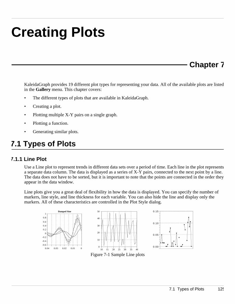
Creating Plots
Chapter 7
listed
resentsy a line. rder they
of e
KaleidaGraph provides 19 different plot types for representing your data. All of the available plots arein the Gallery menu. This chapter covers:
• The different types of plots that are available in KaleidaGraph.
• Creating a plot.
• Plotting multiple X-Y pairs on a single graph.
• Plotting a function.
• Generating similar plots.
7.1 Types of Plots
7.1.1 Line PlotUse a Line plot to represent trends in different data sets over a period of time. Each line in the plot repa separate data column. The data is displayed as a series of X-Y pairs, connected to the next point bThe data does not have to be sorted, but it is important to note that the points are connected in the oappear in the data window.
Line plots give you a great deal of flexibility in how the data is displayed. You can specify the numbermarkers, line style, and line thickness for each variable. You can also hide the line and display only thmarkers. All of these characteristics are controlled in the Plot Style dialog.
Figure 7-1 Sample Line plots
-0.6
-0.4
-0.2
0
0.2
0.4
0.6
0.8
1
00.010.020.030.04
Damped Sine
0
10
20
30
40
50
10 15 20 25 30 35 400.00
0.05
0.10
0.15
7.1 Types of Plots 125

KaleidaGraph
ints are data is
kers o
lot ext poin
d in the
ut witlotting
plot ext poin
d in the
ut wit plottin (Y) axis.
ch linted to thennecte
t, but s usefu (Y) axes
7.1.2 Scatter PlotUse a Scatter plot to compare large sets of data. Scatter plots are similar to Line plots, except the ponot connected by lines. Each X-Y pair is represented by a unique marker on the plot. Each column ofrepresented by a different marker.
Scatter plots display a marker for each point in the plot. It is not possible to display a partial set of marra line between the points. If you want this kind of flexibility, plot the data as a Line plot.
7.1.3 Double Y PlotUse a Double Y plot to display two groups of data, each with its own vertical scale. Each line in the prepresents a separate data column. The data is displayed as a series of X-Y pairs, connected to the ntby a line. The data does not have to be sorted, but it is important to note that the points are connecteorder they appear in the data window.
The Double Y plot gives you the same amount of control over the display of the data as the Line plot, bhthe added capability of having separate scales on the vertical axes. This plot is useful when you are ptwo dependent (Y) groups which share a common independent (X) variable.
7.1.4 Double X PlotUse a Double X plot to display two groups of data, each with its own horizontal scale. Each line in therepresents a separate data column. The data is displayed as a series of X-Y pairs, connected to the ntby a line. The data does not have to be sorted, but it is important to note that the points are connecteorder they appear in the data window.
The Double X plot gives you the same amount of control over the display of the data as the Line plot, bhthe added capability of having separate scales on the horizontal axes. This plot is useful when you aregtwo groups of data that need to have separate independent (X) axes and share the same dependent
7.1.5 Double XY PlotUse a Double XY plot to display two groups of data, each with its own horizontal and vertical scale. Eaein the plot represents a separate data column. The data is displayed as a series of X-Y pairs, connecnext point by a line. The data does not have to be sorted, but it is important to note that the points are codin the order they appear in the data window.
The Double XY plot gives you the same amount of control over the display of the data as the Line plowith the added capability of having two separate scales on the horizontal and vertical axes. This plot ilwhen you are plotting two groups of data that need to have separate independent (X) and dependent
Figure 7-2 Sample Scatter plots
30
40
50
60
708090
100
10-6 10-5 10-4 10-3 10-2 10-1 100
Dose Response
0.01
0.1
1
1 0
-2 -1 0 1 20
2
4
6
8
0 2 4 6 8 10 12 14
Mean
Sample 2896-1
126 7.1 Types of Plots
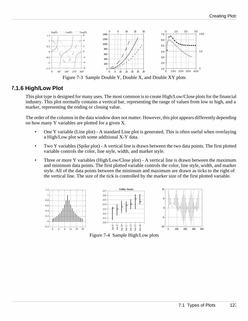
Creating Plots
nancia and a
endin
aying
otte
uarkeht of le.
7.1.6 High/Low PlotThis plot type is designed for many uses. The most common is to create High/Low/Close plots for the filindustry. This plot normally contains a vertical bar, representing the range of values from low to high,marker, representing the ending or closing value.
The order of the columns in the data window does not matter. However, this plot appears differently depgon how many Y variables are plotted for a given X.
• One Y variable (Line plot) - A standard Line plot is generated. This is often useful when overla High/Low plot with some additional X-Y data.
• Two Y variables (Spike plot) - A vertical line is drawn between the two data points. The first pldvariable controls the color, line style, width, and marker style.
• Three or more Y variables (High/Low/Close plot) - A vertical line is drawn between the maximmand minimum data points. The first plotted variable controls the color, line style, width, and mrstyle. All of the data points between the minimum and maximum are drawn as ticks to the rigthe vertical line. The size of the tick is controlled by the marker size of the first plotted variab
Figure 7-3 Sample Double Y, Double X, and Double XY plots
Figure 7-4 Sample High/Low plots
-1.5
-1
-0.5
0
0.5
1
1.5
-6
-4
-2
0
2
4
6
0o 90o 180o 270o 360o
Sin(ϑ ) Cos(ϑ ) Tan(ϑ )
0
200
400
600
800
1000
1200
1400
0 5 10 15 20 25 30
0 5 10 15 20
1 0
2 0
3 0
4 0
5 0
6 0
7 0
1
1 0
100
0 100 200 300 400
0 1 0 2 0 3 0
-0.2
0
0.2
0.4
0.6
0.8
1
1.2
0 4 8 12 16 20
210
211
212
213
214
215
216
217
Jun
8
Jun
9
Jun
10
Jun
11
Jun
12
Jun
15
Jun
16
Utility Stocks
-10
-5
0
5
10
0 100 200 300 400
7.1 Types of Plots 127

KaleidaGraph
ach line not have window
ing the
ility e Y
otted n from ry but
n
lity X is the
7.1.7 Step PlotA Step plot is a variation of a Line plot. It can be used to compare data that does not show a trend. Ein the plot represents a separate data column. The data is plotted as a series of steps. The data doesto be sorted, but it is important to note that the points are connected in the order they appear in the data
Note: It is not possible to display markers on a Step plot. The placement of the steps is controlled usStep Options command (Format menu).
7.1.8 Probability PlotUse a Probability plot to display the graph of a variable normalized to either a linear or normal probabdistribution. The X axis is scaled in probability (between 0 and 100%) and shows the percentage of thvariable whose value is less than the data point. The Y axis displays the range of the data variables.
The Probability plot gives rough information about the local density of the data and symmetry. The pldata points do not coincide, even if there are exact duplicates in the data. It is easy to read informatiothe plot and it can accommodate a large number of observations. The Probability plot is not a summaadisplay of all the data.
Note: The Probability Options command (Format menu) controls whether a linear or normal distributiois used.
7.1.9 X-Y Probability PlotThe X-Y Probability plot is similar to the Probability plot. The only difference is that in an X-Y Probabiplot, you enter the probability associated with each Y value. The data is entered as X-Y pairs, where probability (between 0 and 100%) and Y is the data value.
Figure 7-5 Sample Step plots
Figure 7-6 Sample Probability and X-Y Probability plots
0
2
4
6
8
0 5 10 1550
75
100
125
150
J F M A M J J A S O N D
a
b
c
20
24
28
32
0 20 40 60 80 100
User Response by Age Group
Age
Probability of Response0
5
1 0
1 5
2 0
2 5
0 2 0 4 0 6 0 8 0 1006 8 10 12 14 16 18.01
.1
1
51 0
2 03 0
5 0
7 08 09 09 5
9 9
99.9
99.99
128 7.1 Types of Plots

Creating Plots
ot If more
nd
. Whil A Bo axis they ar
atche the e boxes
If you
7.1.10 Histogram PlotA Histogram calculates the number of data points that fall within a specified bin size. The resulting pldisplays the range of the data on the X axis and the number of data points in each bin on the Y axis. than one variable is plotted, the Y axis displays the total number of points in each bin.
You can use the Histogram Options command (Format menu) to specify the bin size, reference value, anumber of extra bins that get added to the plot. A maximum of 200 bins may be plotted.
7.1.11 Box PlotA Box plot enables you to quickly examine a number of variables and extract their major characteristicsethis does not provide detailed information about the data, it does give you a look at its global behavior.xplot represents each variable as a separate box. The Y axis displays the range of the data and the Xdisplays the names of each variable. See Section D.1 for details on what the boxes represent and howecalculated.
Up to 20 additional variables may (optionally) be overlaid as markers on each plot. The markers are mdone to one with the plotted variables. The first value in a marker column is matched with the first box,second value in a marker column is matched with the second box, and so on. When using markers, thdo not have a fill pattern so that the markers can be clearly identified.
Note: You may not select more than a total of 20 variables and markers from a single data window. rneeds exceed this limit, place the variables and markers in separate data windows.
Figure 7-7 Sample Histogram plots
Figure 7-8 Sample Box plots
0
2
4
6
8
10
0.92
0.94
0.96
0.98
1.00
1.02
1.04
1.06 0
100
200
300
0 20 40 60 80 100 120 140 1600
5
1 0
1 5
2 0
1.2 1.4 1.6 1.8 2
12.8
13.0
13.2
13.4
13.6
A B C D4 0 6 0 8 0 100 120 140 160
A
B
C
Detection Range
Mean•
0
2
4
6
8
1 0
A B C D
7.1 Types of Plots 129

KaleidaGraph
a and th
box. Thpresent patterns
atche the
0 riables
of ategor
ues and
t once.
7.1.12 Percentile PlotA Percentile plot represents each variable as a separate box. The Y axis displays the range of the dateX axis displays the names of each variable. Each box encloses 90% of the data.
The bottom and top of each box represent 5% and 95% of the data. Three lines are drawn inside eachemiddle line represents the median value of the data (50%), while the lower and upper dashed lines re25% and 75% of the data, respectively. Due to the importance of these lines, the boxes do not have fill
Up to 20 additional variables may (optionally) be overlaid as markers on each plot. The markers are mdone to one with the plotted variables. The first value in a marker column is matched with the first box,second value in a marker column is matched with the second box, and so on.
Note: It is not possible to display a fill pattern in the boxes. You may not select more than a total of 2variables and markers from a single data window. If your needs exceed this limit, place the vaand markers in separate data windows.
7.1.13 Horizontal Bar PlotA Horizontal Bar plot is a graph of data selected from one window. The data is displayed as a series horizontal bars. The length of each bar represents the value of a variable. Multiple values for the same cy(row) are displayed as side-by-side bars. The horizontal axis displays the range of the dependent valthe vertical axis displays the categories.
Note: A maximum of one independent (X) variable and 20 dependent (Y) variables may be plotted aCustomizing Horizontal Bar plots is covered in Section 8.15.
Figure 7-9 Sample Percentile plots
Figure 7-10 Sample Horizontal Bar plots
0
2
4
6
8
Test #1 Test #2 Test #3 4 0 6 0 8 0 100 120 140 160
A
B
C
0
2
4
6
8
1 0
A B C D
0 5 10 15 20
10
20
30
40
50
60
70
80
90
100
0 50 100 150 200 250
1995
1996
1997
0 5 10 15 20 25 30 35
JanFebMarApr
MayJunJul
AugSepOctNovDec
130 7.1 Types of Plots

Creating Plots
is Bar plot another. isplays
d at
ertical ry (row) l axis
d at
7.1.14 Stack Bar PlotA Stack Bar plot is a graph of data selected from one window. As in a Horizontal Bar plot, the datadisplayed as a series of horizontal bars. The difference between a Stack Bar plot and a Horizontal is that variables belonging to the same category (row) are displayed as bars stacked one on top ofThe length of each bar represents the sum of the data points for a category. The horizontal axis dthe range of sums for a category and the vertical axis displays the categories.
Note: A maximum of one independent (X) variable and 20 dependent (Y) variables may be plotteonce. Customizing Stack Bar plots is covered in Section 8.15.
7.1.15 Column PlotA Column plot is a graph of data selected from one window. The data is displayed as a series of vbars. The height of each bar represents the value of a variable. Multiple values for the same categoare displayed as side-by-side columns. The horizontal axis displays the categories and the verticadisplays the range of the variables.
Note: A maximum of one independent (X) variable and 20 dependent (Y) variables may be plotteonce. Customizing Column plots is covered in Section 8.15.
Figure 7-11 Sample Stack Bar plots
Figure 7-12 Sample Column plots
0 5 1 0 1 5 2 0 2 5
Jan
Feb
Mar
Apr
-15 -10 -5 0 5 1 0 1 5 2 0
A
B
C
D
E
0 200 400 600 800
1994
1995
1996
1997
New Sales
0
2
4
6
8
10
12
815B
160A
223D
412U
105C
Mis
c
0
5
1 0
1 5
2 0
Jan Feb Mar April
0
10
20
30
-2
-1.5 -1
-0.5 0
0.5 1
1.5
7.1 Types of Plots 131

KaleidaGraph
playeriables eight of
ories and
t once.
d by a data is endent
h of the e plottee nam
7.1.16 Stack Column PlotA Stack Column plot is a graph of data selected from one window. As in a Column plot, the data is disdas a series of vertical bars. The difference between a Stack Column plot and a Column plot is that vabelonging to the same category (row) are displayed as columns stacked one on top of another. The heach bar represents the sum of the data points for a category. The horizontal axis displays the categthe vertical axis displays the range of sums for all variables in that category.
Note: A maximum of one independent (X) variable and 20 dependent (Y) variables may be plotted aCustomizing Stack Column plots is covered in Section 8.15.
7.1.17 Polar PlotIn a Polar plot, the data is plotted on the polar coordinate system. Each point in this system is specifienangle (Ø) in degrees and a radius (R). As an option, an alternate data format can be used, where thespecified in X-Y format and then transformed to the polar coordinate system. In either case, an indepvariable (Ø or X) and one or more dependent variables (R or Y) are selected for plotting.
Using the Polar Options command (Format menu), you can specify the grid type, data format, referenceangle, and direction for Polar plots. Customizing Polar plots is covered in Section 8.16.
7.1.18 Pie ChartA Pie chart displays the value of up to 20 categories as a percentage of the total area of a circle. Eaccategories is represented as a segment of the circle (or a wedge of the pie). Only two variables may bdat one time in a Pie chart. The first is the independent (X) variable or category. This variable contains theof each category. The second variable (Y) contains the category values, which must be numeric.
Figure 7-13 Sample Stack Column plots
Figure 7-14 Sample Polar plots
0
100
200
300
400
500
600
700
800
1996 1997 1998
734.10 709.50
451.00
0
2
4
6
8
10
12
14
815B
160A
223D
412U
105C
Mis
c 0
2
4
6
8
1 0
1 2
Jan Feb Mar Apr
0 cm3
2 cm3
4 cm3
6 cm3
8 cm3
10 cm3
0.000010.00010.0010.010.1
110
0°30°
60°
90°
120°
150°180°
210°
240°
330°
132 7.1 Types of Plots

Creating Plots
izing ata ta or
plays ints to
and al
usefu
ted.
any ploved. The
Note: If more than 20 categories are selected for plotting, only the first 20 appear on the plot. CustomPie charts is covered in Section 8.17. Negative values cannot be plotted in a Pie chart. If the dcontains negative values, a dialog gives you the option of plotting the absolute value of the dacanceling the plot.
7.1.19 Function PlotThe Function plot can be used to display a mathematical function as a plot. Choosing this plot type disadialog where you can enter the function, the minimum and maximum X values, and the number of poplot.
Once the plot is created, it behaves like a Line plot. You have full control over the line style, markers, lother components of the plot. Section 7.3 provides instructions for creating a Function plot.
7.1.20 Text PlotThis plot type allows you to create a plot window whose intended use is text. Text plots are particularlylwhen you want to generate a plot that only contains text, lines, boxes, tables, or pictures.
Note: Certain tools in this window are unavailable, because they can only be used when data is plot
7.1.21 Template PlotThe Template plot is used to generate the same type of plot, using different data. It allows you to take tand use it as a base for plotting new data. This works for both new plots and plots that have been sause of this plot is discussed in Section 7.4.2.
Figure 7-15 Sample Pie charts
Figure 7-16 Sample Function plots
Housing Starts
Jan
Feb
Mar
Apr
May
June
6.98%
19.3%
11%
6.9%26.2%
13.8%
22.8%
0
1
2
3
4
5
6
-50 -25 0 25 50
Y = gaussfit(.5,5,1,10)
-0.4
-0.2
0
0.2
0.4
0.6
0 2 4 6 8 100
20
40
60
80
100
0 20 40 60 80 100
7.1 Types of Plots 133

KaleidaGraph
of the makin
tons a
ht to the datxtracte
7.2 Creating a PlotThe Gallery menu contains the plot types available in KaleidaGraph. You can create a plot using anyopen data windows. If a selection is made in the data you are plotting, only the selected data is used ingthe plot.
To create a plot:
1. Open the data to be plotted.
2. Make any selections in the data windows to plot a subset of the data.
3. Choose a plot type from the Gallery menu. A dialog similar to Figure 7-17 is displayed.
Figure 7-17 Variable Selection dialog
4. Click the appropriate buttons to select the columns to be plotted. You can clear all of the buttonce by clicking the check mark icon in this dialog.
5. Click New Plot to create the plot.
At this point, the plot is linked to the original data window. If another plot is opened, created, or brougthe front, the data for the previous plot becomes embedded in the plot. If the plot is saved, a copy of ais embedded in the plot and saved as part of the plot file. Once data is embedded in a plot, it can be edby choosing Plot > Extract Data or clicking the Find Data button ( ) in the plot window.
134 7.2 Creating a Plot

Creating Plots
ing thisn is usedlot from
in eac
f each from
a set
g this show
7.2.1 Plotting from Multiple Data WindowsUnless you are creating a Pie chart or one of the plots in the Bar submenu, you can plot data from multipledata windows. This is accomplished by making variable selections for each data set to be used.
The Variable Selection dialog contains a pop-up menu listing the names of all open data windows. Usmenu, you can select up to 20 independent and 20 dependent variables to be plotted. If a text columas the independent variable, you may not select any other independent variables and you can only pthat particular data window.
To create a plot from multiple data sets:
1. Open the data to be plotted. To plot subsections of any data sets, select the appropriate rowshdata window.
2. Choose a plot type from the Gallery menu. A Variable Selection dialog appears.
3. Make the independent and dependent variable selections for the active data window.
4. Click the data window’s name in this dialog to display a pop-up menu containing the name odata window. A check mark in front of the name indicates that variables are already selectedthat data window. If the data window contains a data selection, its name is underlined.
The dialog in the background of Figure 7-18 displays the variables selected from the first datand the pop-up menu used to switch between data windows.
Figure 7-18 Variable Selection dialogs
5. Select the name of a different data window and make the variable selections. Continue doinuntil all of the variables to be plotted are selected. The dialog in the foreground of Figure 7-18 sthe selection made from the second data set.
6. Click New Plot to create a plot based on the selections.
7.2 Creating a Plot 135

KaleidaGraph
samele.
penden
he
ntil al for the
7.2.2 Plotting Multiple X-Y Pairs from the Same Data WindowThe Linear, X-Y Probability, and Polar plots allow you to plot multiple independent variables from the data window. If the independent variable is a text column, you may only have one independent variab
For the plot types mentioned above, the Variable Selection dialog contains a pop-up menu listing theindependent variables (X–X9). Using this pop-up menu, you can plot up to nine independent and 20 detvariables from one data window.
To create a plot from one data window, with different X variables:
1. Open the data to be plotted.
2. Choose a plot type from the Gallery menu. A Variable Selection dialog appears.
3. Make the first set of X and Y variable selections.
4. Click the X column’s shadow box to display a pop-up menu containing the list of X variables(X–X9). If one of the variables already contains a selection, it is preceded by a check mark. Tdialog in the background of Figure 7-19 displays the pop-up menu used to select a different independent variable.
Figure 7-19 Variable Selection dialogs
5. Select a different X variable and choose what is to be plotted against it. Continue doing this ulof the selections are made. The dialog in the foreground of Figure 7-19 shows the selectionssecond independent variable.
6. Click New Plot to create a plot based on the selections.
136 7.2 Creating a Plot

Creating Plots
on you
d in define
w lists
on
choose
7.3 Plotting a FunctionKaleidaGraph provides a Function plot that can be used to plot any mathematical function. The functienter is evaluated between the specified limits and is displayed as a plot.
When defining your function, use x for the independent variable. The operators and math functions founFormula Entry can be used in defining your function. Constants and other shorthand references can bedin the library. You can also use any of the definitions included in the Curve Fits folder. The table belosome example definitions:
To create a Function plot:
1. Choose Gallery > Function to display the Function Plot dialog, shown in Figure 7-20.
Figure 7-20 Function Plot dialog
2. Enter the function you want to plot. The File button can be used to load a saved function definiti
3. If necessary, change the values for the minimum, maximum, and number of points.
4. Click New Plot to plot the function.
Once the Function plot is created, it behaves like a Line plot. You have full control over the line style,markers, and all other components of the plot. If you want to see the data generated by the function, Plot > Extract Data or click the Find Data button ( ) in the plot window.
Example Function Definitions
5 * x^2
gaussfit(1, 5, 1, 10)
m1 + m2 * exp(–m3 * x); m1 = 5; m2 = 1; m3 = 0.5
a * exp(–b * x) * cos(c * x + d); a = 4; b = 0.7; c = 2.2; d = 15
7.3 Plotting a Function 137
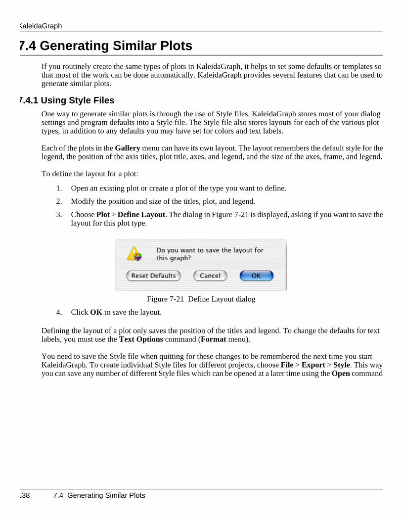
KaleidaGraph
ates so used to
dialog s plot
r th legend.
th
r text
start
7.4 Generating Similar PlotsIf you routinely create the same types of plots in KaleidaGraph, it helps to set some defaults or templthat most of the work can be done automatically. KaleidaGraph provides several features that can begenerate similar plots.
7.4.1 Using Style FilesOne way to generate similar plots is through the use of Style files. KaleidaGraph stores most of your settings and program defaults into a Style file. The Style file also stores layouts for each of the varioutypes, in addition to any defaults you may have set for colors and text labels.
Each of the plots in the Gallery menu can have its own layout. The layout remembers the default style foelegend, the position of the axis titles, plot title, axes, and legend, and the size of the axes, frame, and
To define the layout for a plot:
1. Open an existing plot or create a plot of the type you want to define.
2. Modify the position and size of the titles, plot, and legend.
3. Choose Plot > Define Layout. The dialog in Figure 7-21 is displayed, asking if you want to saveelayout for this plot type.
Figure 7-21 Define Layout dialog
4. Click OK to save the layout.
Defining the layout of a plot only saves the position of the titles and legend. To change the defaults folabels, you must use the Text Options command (Format menu).
You need to save the Style file when quitting for these changes to be remembered the next time you KaleidaGraph. To create individual Style files for different projects, choose File > Export > Style. This wayyou can save any number of different Style files which can be opened at a later time using the Open command
138 7.4 Generating Similar Plots
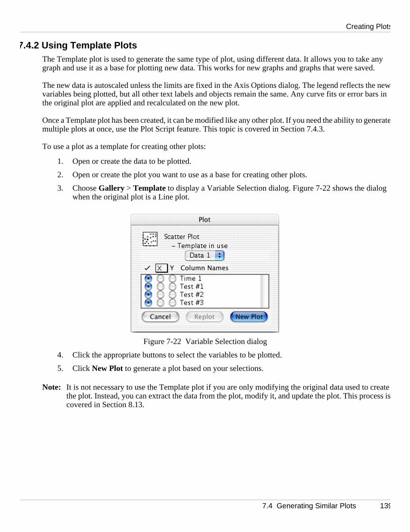
Creating Plots
any ved.
he newars in
enerat
g
create cess is
7.4.2 Using Template PlotsThe Template plot is used to generate the same type of plot, using different data. It allows you to takegraph and use it as a base for plotting new data. This works for new graphs and graphs that were sa
The new data is autoscaled unless the limits are fixed in the Axis Options dialog. The legend reflects tvariables being plotted, but all other text labels and objects remain the same. Any curve fits or error bthe original plot are applied and recalculated on the new plot.
Once a Template plot has been created, it can be modified like any other plot. If you need the ability to gemultiple plots at once, use the Plot Script feature. This topic is covered in Section 7.4.3.
To use a plot as a template for creating other plots:
1. Open or create the data to be plotted.
2. Open or create the plot you want to use as a base for creating other plots.
3. Choose Gallery > Template to display a Variable Selection dialog. Figure 7-22 shows the dialowhen the original plot is a Line plot.
Figure 7-22 Variable Selection dialog
4. Click the appropriate buttons to select the variables to be plotted.
5. Click New Plot to generate a plot based on your selections.
Note: It is not necessary to use the Template plot if you are only modifying the original data used to the plot. Instead, you can extract the data from the plot, modify it, and update the plot. This procovered in Section 8.13.
7.4 Generating Similar Plots 139

KaleidaGraph
ts and e time
controm the
plots.the plo
legen
7.4.3 Using Plot ScriptsAnother way to generate similar plots is the Plot Script command (Windows menu). This feature enables youto choose any plot type or an existing plot and use it as a template for creating multiple plots at once.
When to Use ScriptsThe script feature is intended for the user who has a Template plot and wants to plot different data seview the resulting curves. Even if you only need to generate a simple plot, but you generate it all of thwith different data, you will find plot scripts very useful.
The advantage of a script over a Template plot is that a script can generate multiple plots. Also, you canllegend descriptions and plot titles using a script. In a Template plot, the legend descriptions come frocolumn names of the plotted variables and the plot title remains unchanged.
Creating a Plot ScriptThe Plot Script command is similar to the Template plot but provides you with more options for creatingUsing plot scripts, you can create multiple plots at once, automatically print or save the plots, and set ttitle or legend for each plot.
Choosing Windows > Plot Script displays the dialog in Figure 7-23. This dialog is used to make your selections for the current script. The script selections include: plot type, variable selections, plot titles,dtext, auto print, and auto save options.
Figure 7-23 Plot Script window
140 7.4 Generating Similar Plots
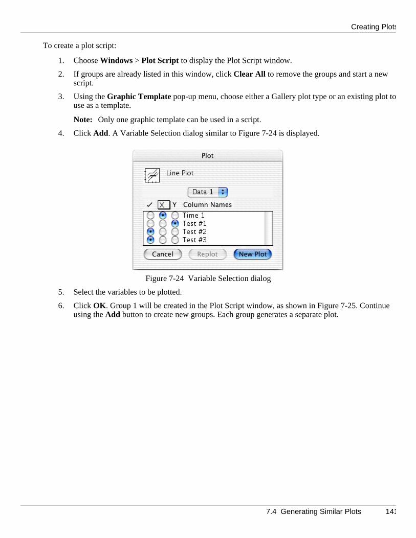
Creating Plots
t to
ue
To create a plot script:
1. Choose Windows > Plot Script to display the Plot Script window.
2. If groups are already listed in this window, click Clear All to remove the groups and start a new script.
3. Using the Graphic Template pop-up menu, choose either a Gallery plot type or an existing plouse as a template.
Note: Only one graphic template can be used in a script.
4. Click Add. A Variable Selection dialog similar to Figure 7-24 is displayed.
Figure 7-24 Variable Selection dialog
5. Select the variables to be plotted.
6. Click OK . Group 1 will be created in the Plot Script window, as shown in Figure 7-25. Continusing the Add button to create new groups. Each group generates a separate plot.
7.4 Generating Similar Plots 141

KaleidaGraph
e plotte
d by a ave a
Figure 7-25 Plot Script window
7. When you are finished creating groups, click Run to execute the script.
Setting Titles and LegendsBy default, the titles are the same as the template and the legend comes from the column names of thdvariables. You can set the plot titles and legends for each plot being created using the Set Titles and Set Legends buttons in the Plot Script window. Clicking either of these buttons displays a text editor.
Each line in the editor corresponds to a different plot. Plot titles are entered on separate lines, followereturn. If you choose to set the titles, you must set them for all of the plots. If a specific plot is not to htitle, create a blank line in the editor by pressing Enter (Windows) or Return (Macintosh). Each title appearsto the right of the corresponding data group in the Plot Script window.
Note: Multi-line titles can be created using the \r characters. Any text that follows \r will be placed on a separate line.
To set the plot titles for a script:
1. Click Set Titles.
2. Enter plot titles as displayed in Figure 7-26.
142 7.4 Generating Similar Plots

Creating Plots
Figure 7-26 Edit Script Titles dialog
3. Choose File > Close. The titles are listed to the right of the groups, as shown in Figure 7-27.
Figure 7-27 Plot Script window after setting titles
7.4 Generating Similar Plots 143

KaleidaGraph
that thr Doubl All
aGraprrect,
olumnata
of X
ays a e screen mark.
The legend information for each plot is also placed on separate lines, followed by a return. To indicate elabels belong to the same plot, each legend label should be separated with either a comma or a tab. FoeY or Double XY plots, enter the labels for the Y1 legend followed by the Y2 labels (on the same line).labels prior to a return belong to the same plot. Only use the Enter (Windows) or Return (Macintosh) key toseparate legend titles associated with different plots.
Note: Multi-line legend labels can be created using the \r characters. Any text that follows \r will be placedon a separate line.
To set the legends for a script:
1. Click Set Legends.
2. Enter legend titles as displayed in Figure 7-28.
Figure 7-28 Edit Script Legends dialog
3. Choose File > Close.
Using Pattern Recognition to Create New GroupsThe Plot Script window includes a pattern recognition feature. Once you add a third data group, Kaleidhtries to identify a pattern in the way you are setting up the groups. If KaleidaGraph’s selections are coyou can replicate the pattern throughout the data window by clicking Repeat instead of OK . KaleidaGraph continues the selection pattern across all of the columns in your data window, and creates the groupsautomatically.
Note: The pattern recognition feature only works across the columns of a data window or across the csof a set of data windows. KaleidaGraph cannot identify a plotting pattern that jumps from one dwindow to another.
Pointing Groups to Different Data WindowsThe Data Windows pop-up menu can be used to select a different data window for each individual setvariable selections. This pop-up menu contains up to 20 X Set menu items (X–X20). A set is defined as an variable and its associated Y variables (such as: X, Y1, Y2). The number of X Set menu items depends on thenumber of independent variables selected for the current group.
The sets are listed in the pop-up menu in the order they were created. Selecting one of the sets displsubmenu containing a list of the open data windows. They are listed in the order they are stacked on th,from front to back. The data window currently associated with a particular set is preceded by a checkFigure 7-29 shows the Plot Script window with the Data Windows pop-up menu and the X Set submenu.
144 7.4 Generating Similar Plots

Creating Plots
ing.
word
tion
Figure 7-29 Selecting different data windows
To change the data window associated with a particular set:
1. Click the group to be edited.
2. Click the Data Windows pop-up menu, select an X Set, and choose a different data window. Theselected data window is now used for that particular set of variable selections.
Note: The only other way to change the data window referenced by a set is to use the Change button after selecting each individual group. This method must be used to select different columns for plott
Exporting Plots AutomaticallyYou can automatically export script-generated plots to the printer or to disk using the Auto Print and Auto Save options.
To automatically print plots:
1. Click the Auto Print check box.
2. Choose either Print Graphics or Print Layout from the pop-up menu immediately below Auto Print .
3. Execute the script by clicking Run. The plots are automatically printed.
To automatically save plots:
1. Click the Auto Save check box.
2. Choose the type of graphic file to be created from the pop-up menu immediately below Auto Save
3. Enter a prefix to be used for the saved plot files. By default, the naming convention uses thePrefix followed by an underscore (_) and a number.
4. Click Run to execute the script. KaleidaGraph displays a dialog allowing you to specify a locafor the saved plots.
7.4 Generating Similar Plots 145
KaleidaGraph
proval.t to anceled
I
ed, the onger
e your
and, om
script.
late. It
cript
Memory ConsiderationsIf KaleidaGraph runs out of memory or you exceed the maximum number of open plot windows whileexecuting a script, the situation is handled based on the current state of the Automatically dispose of old plotsoption in the Preferences dialog (File menu).
When this check box is selected, the oldest plot is discarded from memory, without asking for your apIf this check box is cleared, a dialog asks whether to save or dispose the oldest plot. If you choose nodispose of a plot to make memory available, the request that caused the out of memory condition is c
Saving and Loading ScriptsOnce you have created a script, you can save it to disk by choosing either File > Export > Script or File > Save Script.
If you used an existing plot for the Graphic Template, a plot file is created with the plot script document. nthe Windows version, the plot has the same name as the script, but with a .qpc file name extension. In the Macintosh version, the plot’s file name is the first 25 characters of the script’s file name, followed by .plot. Any future use of the script causes the plot file to open. Once a script and its template have been savplot must remain in the same folder as the script and it cannot be renamed. Otherwise, the script no lrecognizes the plot document.
A default Script file is automatically opened each time KaleidaGraph is started. This way you can savplot script and have it opened the next time you use the program.
Custom Script files can be opened at any time from within KaleidaGraph by choosing File > Import > Scriptor File > Open. The Plot Script window changes to reflect the contents of the new Script file.
7.4.4 Using Formula ScriptsThe last feature that allows you to generate similar plots is a formula script. This feature has a comm#SCRIPT, which has all of the same options as the Plot Script window. You can create a plot script frscratch or you can use a command to open one that is saved.
The advantage of using a formula script is that you can open and modify data windows as part of theYou can also execute more than one plot script inside of a formula script.
The disadvantage of using this feature is that you cannot select a specific plot to be used as the tempmust either be a Gallery plot type or a plot that is opened as part of a saved plot script.
For more information on formula scripts, refer to the following sections:
• Section 6.10.1 explains creating and entering formula scripts.
• Section 6.10.2 discusses the syntax for the #SCRIPT command and the rest of the formula scommands.
• Section 6.10.3 contains some example formula scripts.
146 7.4 Generating Similar Plots

Working with Plots
Chapter 8
, axes,
se
b
KaleidaGraph provides complete control over the appearance of your plots. This includes the legendticks, grid lines, and labels, in addition to how the data is represented on the plot.
This chapter explains how to:
• Edit the legend and legend text.
• Change the axis limits and scaling, as well as removing, exchanging, and linking axes.
• Control the display and number of tick marks.
• Control the display of grid lines.
• Control the display of axis labels.
• Change the marker, fill pattern, line style, line width, and variable color.
• Change the frame, grid, interior, and background colors of a plot.
• Resize the plot.
• Change the data in a plot.
• Customize Bar, Polar, and Pie plots.
8.1 Hiding, Displaying, and Closing PlotsThe Windows menu contains four commands that can be used to hide and display plot windows. Thecommands operate on either a single window or all of the plot windows at once.
8.1.1 Changing the Active WindowTo make a plot window active, click anywhere in the desired plot window or choose Windows > Show Plotand select its name.
8.1.2 Hiding Plot WindowsTo hide a plot window, choose Windows > Hide Window and select its name. You can hide all open plots ychoosing Windows > Hide All Plots.
8.1 Hiding, Displaying, and Closing Plots 147

KaleidaGraph
. The
.
d try tos. The
the
ge thnd
300, and
8.1.3 Displaying Plot WindowsYou can display a hidden plot window with the Show Plot command (Windows menu). The names of hiddenplot windows appear in italic. Select the name of the desired plot window and it is brought to the frontShow All Plots command can be used to display all of the plot windows at once.
8.1.4 Closing Plot WindowsYou can use the Close All Plots command (Windows menu) to close all of the open plot windows at onceIndividual plot windows can be closed by choosing File > Close or clicking the close box of each window. Adialog may be displayed, asking if you want to save the plot before closing.
Note: If you do not want to save the plot, this dialog can be avoided by pressing Shift while either clicking the close box or choosing File > Close/NoSave.
You can have a maximum of 32 plots open at one time in KaleidaGraph. If you have 32 plots open ancreate another plot, either the oldest plot is automatically disposed or the dialog in Figure 8-1 appearPreferences dialog (File menu) contains an option that controls the automatic disposal of plots. If Automatically dispose of old plots is selected, the oldest plot is discarded. If this check box is cleared,dialog is displayed.
Figure 8-1 Maximum Open Plots dialog
8.2 Changing the View of the Plot WindowKaleidaGraph provides several magnification levels for changing the view of the plot window. To chanemagnification of the plot, click the Zoom drop-down menu in the lower-left corner of the plot window achoose the desired zoom level. The available zoom percentages are: 25, 50, 75, 100, 125, 150, 200,400%.
8.3 Displaying Rulers and Grids in the Plot WindowTo turn the rulers and grids on and off in the plot window:
1. With the plot window active, choose Plot > Ruler & Grids .
2. Click the appropriate check boxes to display the rulers, grids, or both.
3. Select the proper units that you want to use.
4. Click OK to return to the plot window.
148 8.2 Changing the View of the Plot Window

Working with Plots
plot. Byables in
e elect d colo
ttes
n outeontrols
rs wheround
8.4 Modifying the LegendThe legend consists of a frame, the plot symbols, and the labels used to identify each variable in the default, the labels are taken from the column names in the data window. The legend displays the varithe order they are selected for plotting.
8.4.1 Editing the Legend Frame and ColorChanging Foreground and Background ColorThe Color icon on the toolbox consists of two sections: a foreground section (upper left) for setting thforeground color and a background section (lower right) for setting the background color. When you safill or pen pattern, the foreground color is applied to the black portion of the pattern and the backgrounris applied to the white portion of the pattern.
To change the foreground or background color of the legend:
1. Click the legend to select it.
2. Click the foreground or background section of the Color icon. One of the following color paleappears with the current color choices.
3. Select a different color from the palette.
Changing Fill and Pen PatternsThe Pattern icon on the toolbox consists of two sections: an inner section for setting the fill pattern and arsection for setting the pen pattern. The fill pattern controls the interior of the legend; the pen pattern cthe legend frame.
You can change the fill or pen pattern by selecting a different pattern from the pop-up menu that appeanyou click the appropriate portion of the Pattern icon. Black portions of the pattern represent the foregcolor and white portions represent the background color.
Figure 8-2 Foreground Color palette Figure 8-3 Background Color palette
8.4 Modifying the Legend 149
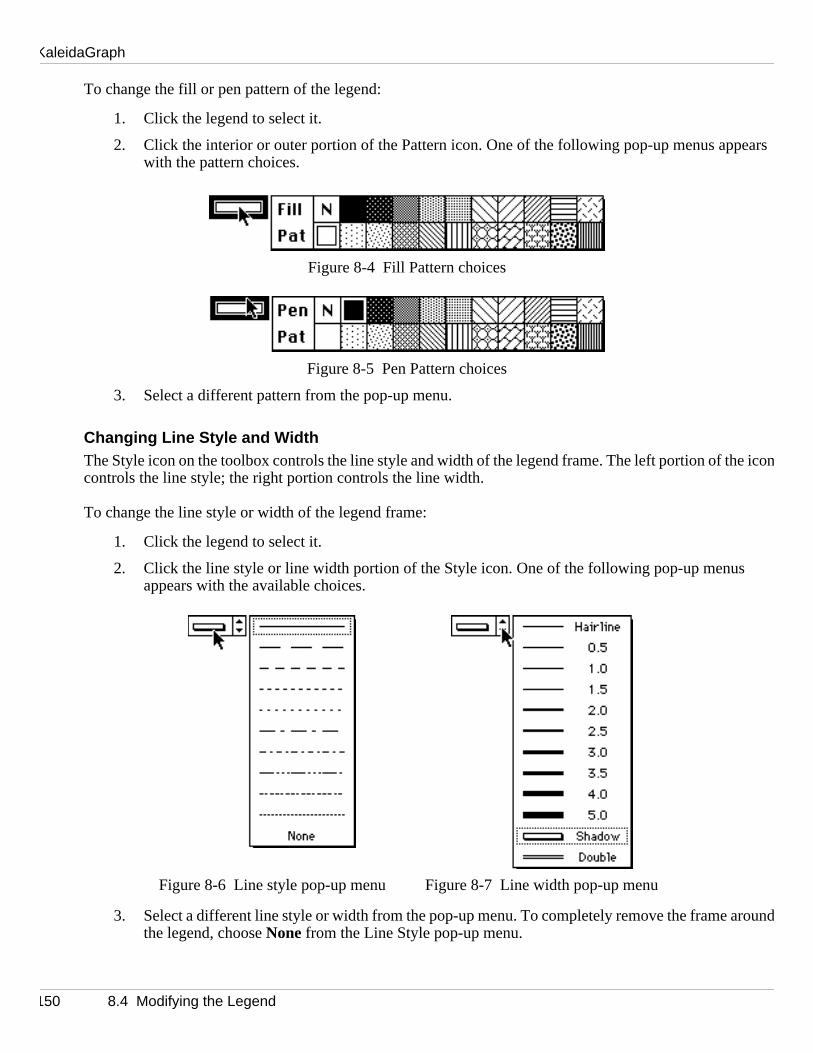
KaleidaGraph
ears
e ico
roun
To change the fill or pen pattern of the legend:
1. Click the legend to select it.
2. Click the interior or outer portion of the Pattern icon. One of the following pop-up menus appwith the pattern choices.
Figure 8-4 Fill Pattern choices
Figure 8-5 Pen Pattern choices
3. Select a different pattern from the pop-up menu.
Changing Line Style and WidthThe Style icon on the toolbox controls the line style and width of the legend frame. The left portion of thncontrols the line style; the right portion controls the line width.
To change the line style or width of the legend frame:
1. Click the legend to select it.
2. Click the line style or line width portion of the Style icon. One of the following pop-up menus appears with the available choices.
3. Select a different line style or width from the pop-up menu. To completely remove the frame adthe legend, choose None from the Line Style pop-up menu.
Figure 8-6 Line style pop-up menu Figure 8-7 Line width pop-up menu
150 8.4 Modifying the Legend

Working with Plots
bere
legen only
labels.
t Strin
by
thes
Setting Legend Frame DefaultsTo make the current legend style the default, choose Plot > Define Layout. Choosing this command only remembers the settings for this particular type of plot because each plot type in the Gallery menu can have itsown layout.
This information is saved as part of the Style file. You must save the Style file for the layout to be rememdthe next time you start KaleidaGraph.
8.4.2 Editing Legend TextEditing Legend Text Attributes as a GroupThe attributes of the legend text can be changed as a group by double-clicking any of the labels in thedwith the Selection Arrow. A variation of the Edit String dialog, shown in Figure 8-8, appears which canbe used to modify the attributes of the text labels. This dialog does not allow you to edit any of the textSee Section 9.7.4 for more information on the commands available in this dialog.
Figure 8-8 Variation of Edit String dialog
Editing Individual Items in the LegendThe labels in the legend can be edited using the Text tool. Double-clicking a text label displays the Edigdialog. Edit the legend text as needed and click OK to return to the plot.
The labels in the legend can be moved to different locations using the Text tool. This is accomplisheddragging a label to a new position with the Text tool. To delete an item in the legend, use the Eraser.
Changing Legend Text Color Independent of Variable ColorBy default, the color of the legend text is linked to the variable color set in the Plot Style dialog. To makeedifferent colors, choose Format > Text Options and clear the Link Text To Variable Color check box. Thetext and variable colors can now be set independently.
8.4 Modifying the Legend 151
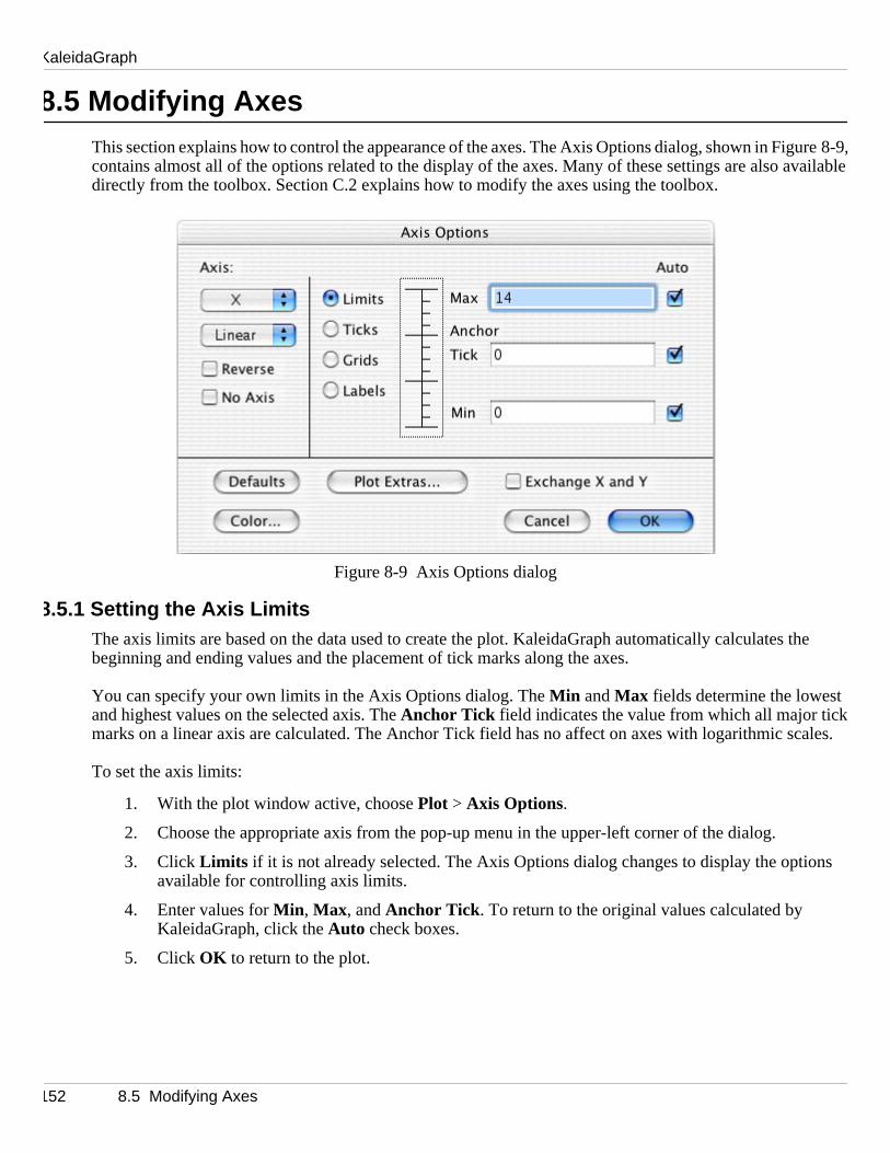
KaleidaGraph
ure 8-9vailable
the
ales.
ns
8.5 Modifying AxesThis section explains how to control the appearance of the axes. The Axis Options dialog, shown in Fig,contains almost all of the options related to the display of the axes. Many of these settings are also adirectly from the toolbox. Section C.2 explains how to modify the axes using the toolbox.
Figure 8-9 Axis Options dialog
8.5.1 Setting the Axis LimitsThe axis limits are based on the data used to create the plot. KaleidaGraph automatically calculates beginning and ending values and the placement of tick marks along the axes.
You can specify your own limits in the Axis Options dialog. The Min and Max fields determine the lowest and highest values on the selected axis. The Anchor Tick field indicates the value from which all major tickmarks on a linear axis are calculated. The Anchor Tick field has no affect on axes with logarithmic sc
To set the axis limits:
1. With the plot window active, choose Plot > Axis Options.
2. Choose the appropriate axis from the pop-up menu in the upper-left corner of the dialog.
3. Click Limits if it is not already selected. The Axis Options dialog changes to display the optioavailable for controlling axis limits.
4. Enter values for Min , Max, and Anchor Tick . To return to the original values calculated by KaleidaGraph, click the Auto check boxes.
5. Click OK to return to the plot.
152 8.5 Modifying Axes

Working with Plots
f yor.
lot.
their d Pi
electinlecte
8.5.2 Selecting Linear or Log ScalingThe numeric axes in KaleidaGraph can have either linear or logarithmic scaling. When Linear scaling is selected, the axis is divided into equal sections. When Log scaling is used, each increment of the axis is apower of 10. Partial decades are allowed when using the log scale.
To change the scaling of an axis:
1. With the plot window active, choose Plot > Axis Options.
2. Choose the appropriate axis from the pop-up menu in the upper-left corner of the dialog.
3. Choose Linear or Log from the pop-up menu beneath the menu used to select the axis.
Note: The Min value in the Axis Options dialog must be greater than zero to use log scaling. Iutry to use non-positive limits, a message appears and the axis scaling reverts to linea
4. Click OK to return to the plot.
8.5.3 Hiding an AxisIt is possible to hide each of the four axes in a plot using the No Axis option in the Axis Options dialog.
To hide an axis:
1. With the plot window active, choose Plot > Axis Options.
2. Choose the appropriate axis from the pop-up menu in the upper-left corner of the dialog.
3. Click the No Axis check box.
4. Click OK to return to the plot.
8.5.4 Exchanging AxesThe Exchange X and Y option in the Axis Options dialog can be used to swap the X and Y axes of a pWhen this check box is selected, the X and X2 axes switch position with the Y and Y2 axes.
Note: Using this option does not change the independent and dependent variables. It only changes position in the plot. This option has no affect on Double Y, Double X, Double XY, Bar, Polar, aneplots.
To exchange the X and Y axes:
1. With the plot window active, choose Plot > Axis Options.
2. Click the Exchange X and Y check box.
3. Click OK to return to the plot.
8.5.5 Reversing the Variables on an AxisYou can control whether the variables are plotted in ascending or descending order along an axis. By sgthe Reverse check box in the Axis Options dialog, variables are plotted in descending order along the sedaxis.
8.5 Modifying Axes 153

KaleidaGraph
XY
not
of thethe X
To reverse an axis on the plot:
1. With the plot window active, choose Plot > Axis Options.
2. Choose the appropriate axis from the pop-up menu in the upper-left corner of the dialog.
3. Click the Reverse check box.
4. Click OK to return to the plot.
8.5.6 Linking a Second AxisYou can control the display of the tick marks and labels on the X2 and Y2 axes using the Link To pop-up menu. This pop-up menu only appears in the Axis Options dialog when the X2 or Y2 axis is selected.
Note: The Link To pop-up menu is not displayed for certain axes in Double Y, Double X, and Doubleplots because they are independent of the main axis.
To link the X2 or Y2 axis:
1. With the plot window active, choose Plot > Axis Options.
2. Choose the X2 or Y2 axis from the pop-up menu in the upper-left corner of the dialog.
3. From the Link To pop-up menu, select how the axis should be linked. The options include:
• No Ticks, No Labels - The X2 or Y2 axis does not have any ticks or labels.
• Axis, No Labels - The X2 or Y2 axis has the same tick marks as the main axis, but does have any labels.
• Axis, Labels - The X2 or Y2 axis has the same tick marks and labels as the main axis.
• Custom Axis, Custom Labels - Depending on the scaling of the main axis, the X2 or Y2 axis is linked by either a linear or exponential equation. The equation is entered into onedialogs shown in Figure 8-10. The tick marks and labels are calculated and displayed on 2or Y2 axis.
4. Click OK to return to the plot.
Figure 8-10 Define Axis Formula dialogs
154 8.5 Modifying Axes

Working with Plots
r, ther
n in ettings the
8.5.7 Changing Axis ThicknessTo change the thickness of the axes:
1. Choose Format > Plot Extras.
2. To increase the thickness, change the Frame Thickness to 200, 300, or 400%.
Note: Depending on the value entered, you may not notice the change on the screen; howeveewill be a difference when the plot is printed.
3. Click OK to return to the plot.
8.6 Modifying Tick MarksThis section explains how to change the appearance of the tick marks. The Axis Options dialog, showFigure 8-11, contains almost all of the options related to the display of the tick marks. Many of these sare also available directly from the toolbox. Section C.2.4 explains how to modify the tick marks usingtoolbox.
Figure 8-11 Axis Options dialog
8.6 Modifying Tick Marks 155

KaleidaGraph
choose
ajo
men
ajo
u.
a fixe
8.6.1 Changing the Display of Tick MarksThe major and minor ticks can be displayed inside, outside, or on both sides of the axis. You can alsonot to display them at all.
To control how the major and minor ticks are displayed:
1. With the plot window active, choose Plot > Axis Options.
2. Choose the appropriate axis from the pop-up menu in the upper-left corner of the dialog.
3. Click Ticks. The Axis Options dialog changes to display the options available for controlling mrand minor ticks.
4. Choose In , Out, Both, or None from the pop-up menus below Major and Minor to specify how themajor and minor ticks should be displayed.
5. Click OK to return to the plot.
Figure 8-12 shows how the tick marks appear when you select (in order): In , Out, Both, and None for the Xand Y axes.
Figure 8-12 Tick mark display
8.6.2 Changing the Number of Tick MarksWhen Linear scaling is selected for an axis, the number of major tick marks is controlled by the pop-uputo the right of Major in the Axis Options dialog. They can either be calculated automatically or set to aspecific number.
To change the number of major ticks:
1. With the plot window active, choose Plot > Axis Options.
2. Choose the appropriate axis from the pop-up menu in the upper-left corner of the dialog.
3. Click Ticks. The Axis Options dialog changes to display the options available for controlling mrand minor ticks.
4. Choose Auto or Fixed # from the pop-up menu to the right of Major .
5. If Fixed # is selected, enter the desired number of divisions in the field below the pop-up men
6. Click OK to return to the plot.
The number of minor tick marks is controlled in the same manner as major ticks. You can either specifydnumber or let KaleidaGraph calculate the number of minor ticks.
156 8.6 Modifying Tick Marks

Working with Plots
ajor along
ns
.
a
r, ther
in s are olbox
8.6.3 Changing the Tick Mark IntervalWhen Linear scaling is selected for an axis, KaleidaGraph automatically determines the number of mtick marks. Using the Axis Options command, it is possible to place the tick marks at specific intervalsan axis.
To change the interval between major tick marks:
1. With the plot window active, choose Plot > Axis Options.
2. Choose the appropriate axis from the pop-up menu in the upper-left corner of the dialog.
3. Click Limits if it is not already selected. The Axis Options dialog changes to display the optioavailable for controlling axis limits.
4. Enter a value in the Anchor Tick field. The intervals are calculated from the Anchor Tick value
5. Click Ticks.
6. Choose Interval from the pop-up menu to the right of Major and enter the desired interval in thefield below it. For dates, enter the desired number of days for the interval. For time data, useD:H:M:S.S format for entering the interval.
7. Click OK to return to the plot.
8.6.4 Changing Tick Mark Length or ThicknessTo change the length or thickness of the tick marks:
1. Choose Format > Plot Extras.
2. To change the length, edit the Inside and Outside values for Major or Minor .
3. To increase the thickness, change the Tick Thickness to 200, 300, or 400%.
Note: Depending on the value entered, you may not notice the change on the screen; howeveewill be a difference when the plot is printed.
4. Click OK to return to the plot.
8.7 Modifying Grid LinesThis section explains how to control the appearance of the grid lines. The Axis Options dialog, shownFigure 8-13, contains most of the options related to the display of the grid lines. Many of these settingalso available directly from the toolbox. Section C.2.5 explains how to modify the grid lines using the to
8.7 Modifying Grid Lines 157

KaleidaGraph
otted),
ajo
r, ther
Figure 8-13 Axis Options dialog
8.7.1 Controlling the Display of Grid LinesGrid lines can be displayed at each of the major and minor tick marks. The lines can be solid, gray (dor not displayed at all. Section 8.10 explains how to change the color of the grid lines.
To control how the grid lines are displayed:
1. With the plot window active, choose Plot > Axis Options.
2. Choose the appropriate axis from the pop-up menu in the upper-left corner of the dialog.
3. Click Grids. The Axis Options dialog changes to display the options available for controlling mrand minor grids.
4. Choose Solid, Gray, or None from the pop-up menus to the right of Major and Minor to specify how the major and minor grids should be displayed.
5. Click OK to return to the plot.
8.7.2 Changing Grid Line ThicknessTo change the thickness of the grid lines:
1. Choose Format > Plot Extras.
2. To increase the thickness, change the Grid Thickness to 200, 300, or 400%.
Note: Depending on the value entered, you may not notice the change on the screen; howeveewill be a difference when the plot is printed.
3. Click OK to return to the plot.
158 8.7 Modifying Grid Lines
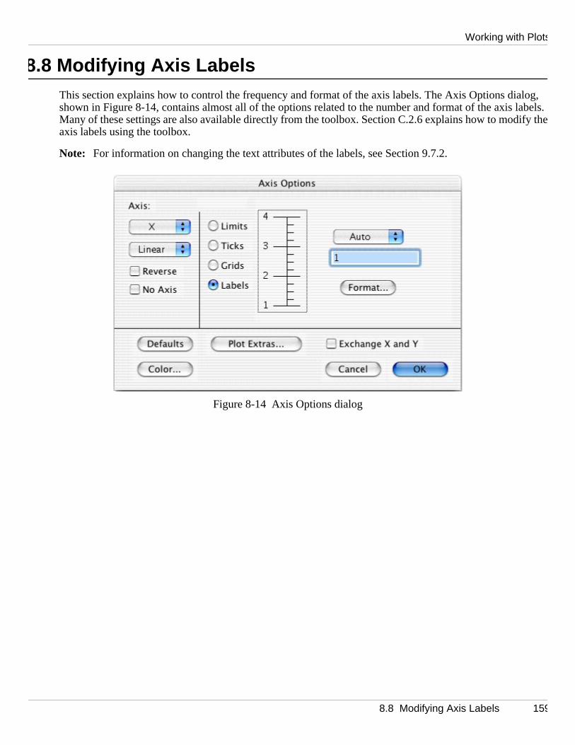
Working with Plots
log, labels. ify th
8.8 Modifying Axis LabelsThis section explains how to control the frequency and format of the axis labels. The Axis Options diashown in Figure 8-14, contains almost all of the options related to the number and format of the axis Many of these settings are also available directly from the toolbox. Section C.2.6 explains how to modeaxis labels using the toolbox.
Note: For information on changing the text attributes of the labels, see Section 9.7.2.
Figure 8-14 Axis Options dialog
8.8 Modifying Axis Labels 159
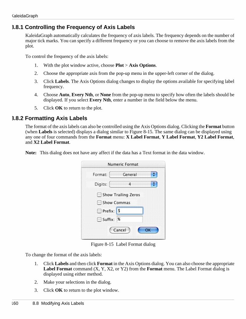
KaleidaGraph
mber oom th
abel
b
using
iat
8.8.1 Controlling the Frequency of Axis LabelsKaleidaGraph automatically calculates the frequency of axis labels. The frequency depends on the nufmajor tick marks. You can specify a different frequency or you can choose to remove the axis labels freplot.
To control the frequency of the axis labels:
1. With the plot window active, choose Plot > Axis Options.
2. Choose the appropriate axis from the pop-up menu in the upper-left corner of the dialog.
3. Click Labels. The Axis Options dialog changes to display the options available for specifying lfrequency.
4. Choose Auto, Every Nth, or None from the pop-up menu to specify how often the labels shouldedisplayed. If you select Every Nth, enter a number in the field below the menu.
5. Click OK to return to the plot.
8.8.2 Formatting Axis LabelsThe format of the axis labels can also be controlled using the Axis Options dialog. Clicking the Format button(when Labels is selected) displays a dialog similar to Figure 8-15. The same dialog can be displayed any one of four commands from the Format menu: X Label Format, Y Label Format, Y2 Label Format, and X2 Label Format.
Note: This dialog does not have any affect if the data has a Text format in the data window.
Figure 8-15 Label Format dialog
To change the format of the axis labels:
1. Click Labels and then click Format in the Axis Options dialog. You can also choose the appropreLabel Format command (X, Y, X2, or Y2) from the Format menu. The Label Format dialog is displayed using either method.
2. Make your selections in the dialog.
3. Click OK to return to the plot window.
160 8.8 Modifying Axis Labels

Working with Plots
hownse using
ppear
th
8.9 Modifying Lines, Markers, and Fill PatternsThis section explains how to control the display of the data in the plot window. The Plot Style dialog, sin Figure 8-16, contains most of the options available for the display of the plot variables. Many of thesettings are also available directly from the toolbox. Section C.3 explains how to modify the plot stylethe toolbox.
Figure 8-16 Plot Style dialog
8.9.1 Selecting Variables in the Plot Style DialogBefore variables can be modified, they need to be selected in the Plot Style dialog. Each variable is independently controlled in this dialog.
To select variables for editing in the Plot Style dialog:
1. With the plot window active, choose Plot > Plot Style.
2. Use the and buttons to locate the desired variable. The name of the current variable asto the right of these buttons.
Note: The Tab and Down Arrow keys can be used to move to the next variable. You can go toeprevious variable using Shift+Tab or the Up Arrow key. The Left Arrow key takes you tothe first variable; the Right Arrow key takes you to the last variable.
8.9 Modifying Lines, Markers, and Fill Patterns 161
KaleidaGraph
ck Bar,played
arkers
Line
8.9.2 Changing Marker Type, Size, or Number of MarkersMost of the plots have the ability to display markers on the plot. The exceptions are the Histogram, StaStack Column, and Pie plots. The Plot Style dialog controls the type, size, and number of markers disin the plot.
To change the marker type, size, or number of markers:
1. With the plot window active, choose Plot > Plot Style.
2. Select the variable to be edited. See Section 8.9.1 if you are unsure of how to do this.
3. To change the marker type, click one of the symbols below Marker . The first six markers in the leftcolumn are transparent; all of the others are opaque. The active marker has a box around it.
4. To change the size of the marker, edit the value in the Marker Size field.
5. To change the number of markers displayed, make a selection from the Show Markers pop-up menu. You can choose whether all, a fixed number, a percentage, every Nth, or none of the mare displayed on the plot. The current setting is preceded by a check mark.
Note: Scatter plots always show all of the markers. Use a Line plot to show fewer markers.
6. Click OK to return to the plot.
8.9.3 Selecting Fill PatternsAll of the plots have the ability to have a fill pattern displayed for the variable. For some plots, like theplot, this is only possible if Bar is selected as the marker type in the Plot Style dialog.
Note: It is not possible to assign a fill pattern to the markers.
To change the fill pattern:
1. With the plot window active, choose Plot > Plot Style.
2. Select the variable to be edited. See Section 8.9.1 if you are unsure of how to do this.
3. Click one of the patterns below Fill Pattern . The active fill pattern has a box around it.
4. Click OK to return to the plot.
162 8.9 Modifying Lines, Markers, and Fill Patterns

Working with Plots
all of et usin
olor
quare
it lines.Line lines.
r, ther
8.9.4 Changing Appearance of Variable and Curve Fit LinesLine, Double Y, Double X, Double XY, High/Low, Step, Probability, X-Y Probability, Horizontal Bar, Column, and Function plots can use a line to represent a plotted variable. Curve fits can be applied tothese plots as well as Scatter plots. The style, width, and color of the variable or curve fit lines can be sgthe Plot Style dialog.
Note: Variable and curve fit lines are controlled independently of each other. Changing the variable calso changes the marker color. The associated legend text is also changed if Link Text To Variable Color is selected in the Text Options dialog (Format menu).
To change the line style, width, or color of variable or curve fit lines:
1. With the plot window active, choose Plot > Plot Style.
2. Select the variable to be edited. See Section 8.9.1 if you are unsure of how to do this.
3. If changes are being made to the variable line, proceed to the next step. Otherwise, click Curve Fitto make changes to the curve fit line.
4. To change the line style, select a different option from the Style column. Choose None from this list to hide the line. The current style is preceded by a check mark.
5. To change the line width, select a different option from the Width column. The current width is preceded by a check mark.
Note: If you also want to make the markers thicker, follow the instructions in Section 8.9.5.
6. To change the color, select a different color from the palette. The current color has a white saround it.
7. Click OK to return to the plot.
8.9.5 Changing Marker and Line ThicknessThe Plot Style dialog contains a number of options for setting the thickness of the variable and curve fHowever, this setting does not affect the thickness of the markers. The Plot Extras dialog contains a Thickness setting that can be used to increase the thickness of markers, variable lines, and curve fit
To change the thickness of the markers, variable lines, and curve fit lines:
1. Choose Format > Plot Extras.
2. To increase the thickness, change the Line Thickness to 200, 300, or 400%.
Note: Depending on the value entered, you may not notice the change on the screen; howeveewill be a difference when the plot is printed.
3. Click OK to return to the plot.
8.9 Modifying Lines, Markers, and Fill Patterns 163
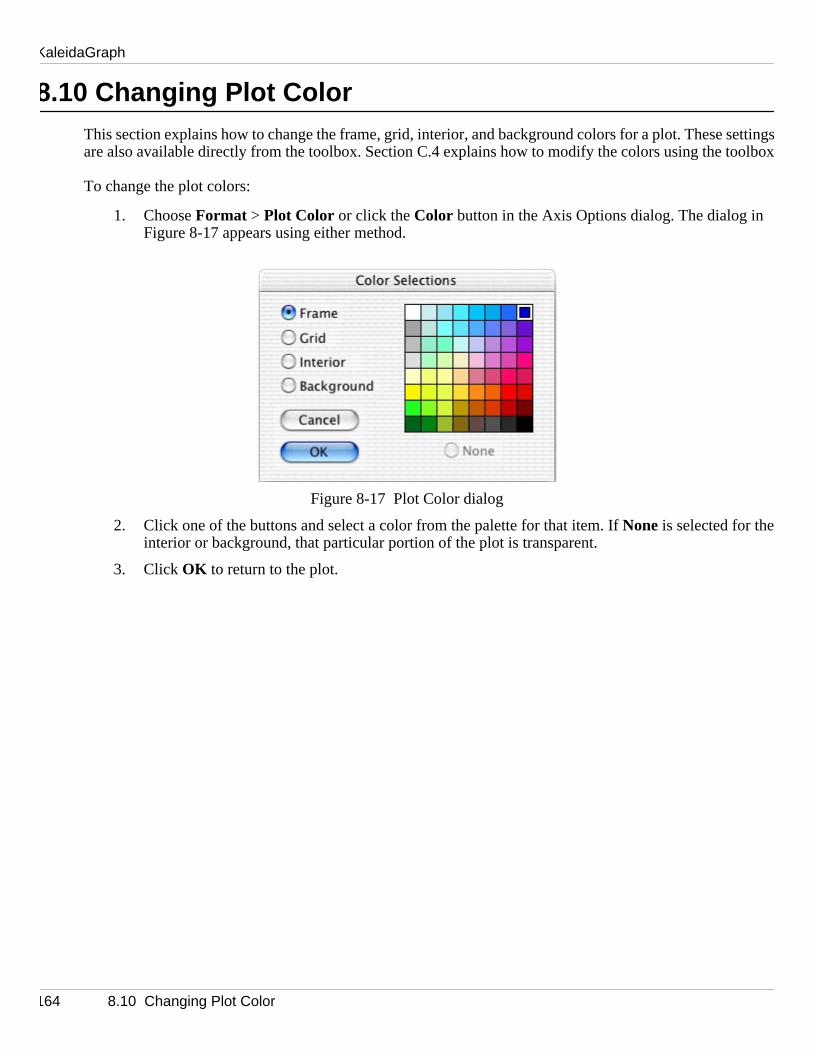
KaleidaGraph
settingsolbox
8.10 Changing Plot ColorThis section explains how to change the frame, grid, interior, and background colors for a plot. These are also available directly from the toolbox. Section C.4 explains how to modify the colors using the to
To change the plot colors:
1. Choose Format > Plot Color or click the Color button in the Axis Options dialog. The dialog in Figure 8-17 appears using either method.
Figure 8-17 Plot Color dialog
2. Click one of the buttons and select a color from the palette for that item. If None is selected for the interior or background, that particular portion of the plot is transparent.
3. Click OK to return to the plot.
164 8.10 Changing Plot Color
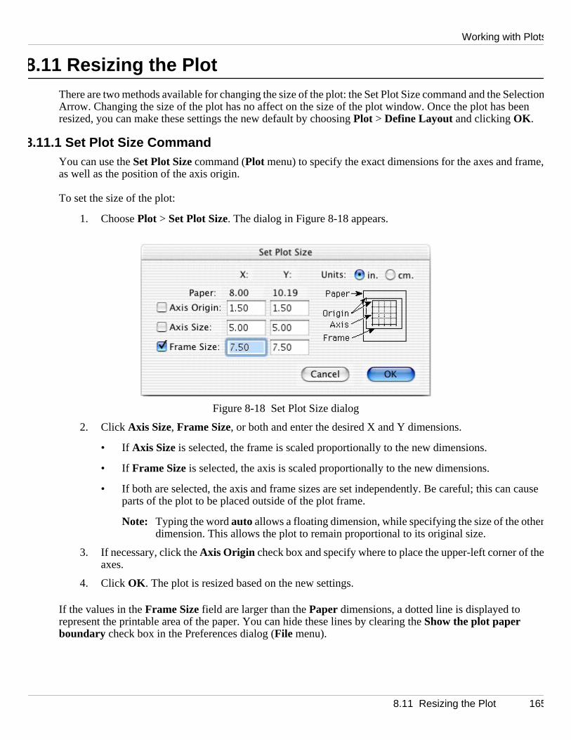
Working with Plots
electioeen
me,
cause
e
th
8.11 Resizing the PlotThere are two methods available for changing the size of the plot: the Set Plot Size command and the SnArrow. Changing the size of the plot has no affect on the size of the plot window. Once the plot has bresized, you can make these settings the new default by choosing Plot > Define Layout and clicking OK .
8.11.1 Set Plot Size CommandYou can use the Set Plot Size command (Plot menu) to specify the exact dimensions for the axes and fraas well as the position of the axis origin.
To set the size of the plot:
1. Choose Plot > Set Plot Size. The dialog in Figure 8-18 appears.
Figure 8-18 Set Plot Size dialog
2. Click Axis Size, Frame Size, or both and enter the desired X and Y dimensions.
• If Axis Size is selected, the frame is scaled proportionally to the new dimensions.
• If Frame Size is selected, the axis is scaled proportionally to the new dimensions.
• If both are selected, the axis and frame sizes are set independently. Be careful; this canparts of the plot to be placed outside of the plot frame.
Note: Typing the word auto allows a floating dimension, while specifying the size of the othrdimension. This allows the plot to remain proportional to its original size.
3. If necessary, click the Axis Origin check box and specify where to place the upper-left corner ofeaxes.
4. Click OK . The plot is resized based on the new settings.
If the values in the Frame Size field are larger than the Paper dimensions, a dotted line is displayed to represent the printable area of the paper. You can hide these lines by clearing the Show the plot paper boundary check box in the Preferences dialog (File menu).
8.11 Resizing the Plot 165
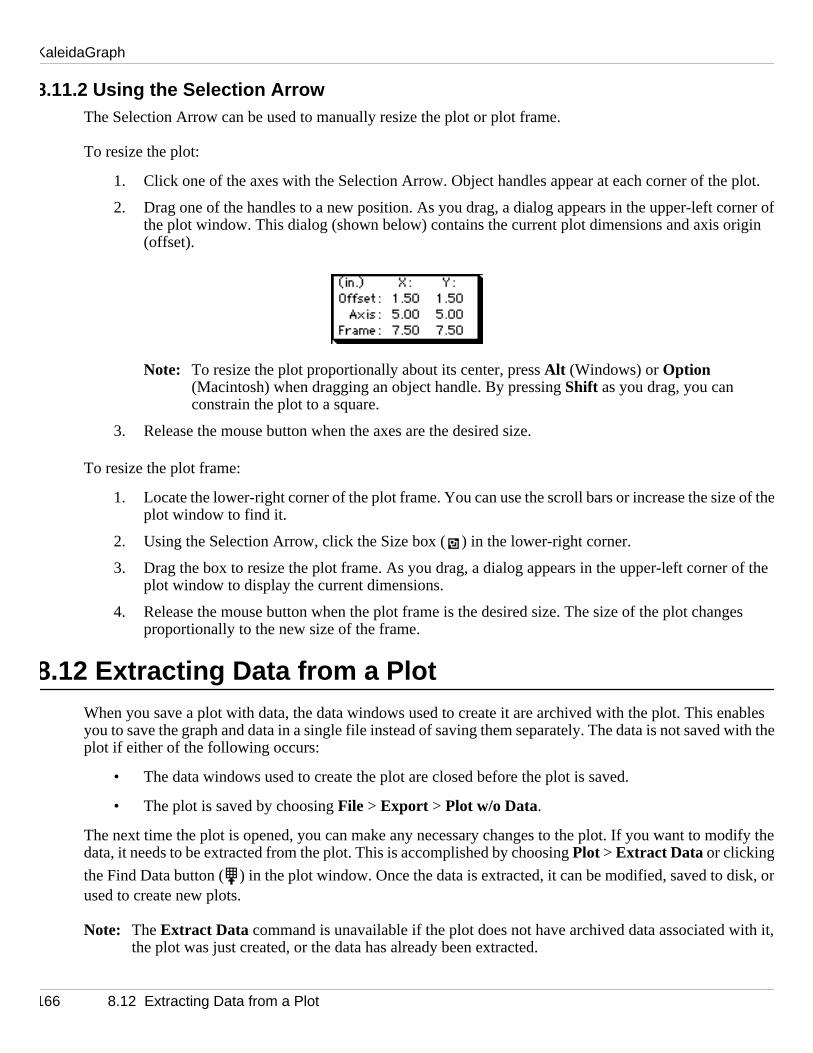
KaleidaGraph
plot.
rner ogin
e of th
of the
ges
ables with th
dify the
isk, o
ith it,
8.11.2 Using the Selection ArrowThe Selection Arrow can be used to manually resize the plot or plot frame.
To resize the plot:
1. Click one of the axes with the Selection Arrow. Object handles appear at each corner of the
2. Drag one of the handles to a new position. As you drag, a dialog appears in the upper-left cofthe plot window. This dialog (shown below) contains the current plot dimensions and axis ori(offset).
Note: To resize the plot proportionally about its center, press Alt (Windows) or Option (Macintosh) when dragging an object handle. By pressing Shift as you drag, you can constrain the plot to a square.
3. Release the mouse button when the axes are the desired size.
To resize the plot frame:
1. Locate the lower-right corner of the plot frame. You can use the scroll bars or increase the sizeplot window to find it.
2. Using the Selection Arrow, click the Size box ( ) in the lower-right corner.
3. Drag the box to resize the plot frame. As you drag, a dialog appears in the upper-left corner plot window to display the current dimensions.
4. Release the mouse button when the plot frame is the desired size. The size of the plot chanproportionally to the new size of the frame.
8.12 Extracting Data from a PlotWhen you save a plot with data, the data windows used to create it are archived with the plot. This enyou to save the graph and data in a single file instead of saving them separately. The data is not savedeplot if either of the following occurs:
• The data windows used to create the plot are closed before the plot is saved.
• The plot is saved by choosing File > Export > Plot w/o Data.
The next time the plot is opened, you can make any necessary changes to the plot. If you want to modata, it needs to be extracted from the plot. This is accomplished by choosing Plot > Extract Data or clicking
the Find Data button ( ) in the plot window. Once the data is extracted, it can be modified, saved to drused to create new plots.
Note: The Extract Data command is unavailable if the plot does not have archived data associated wthe plot was just created, or the data has already been extracted.
166 8.12 Extracting Data from a Plot
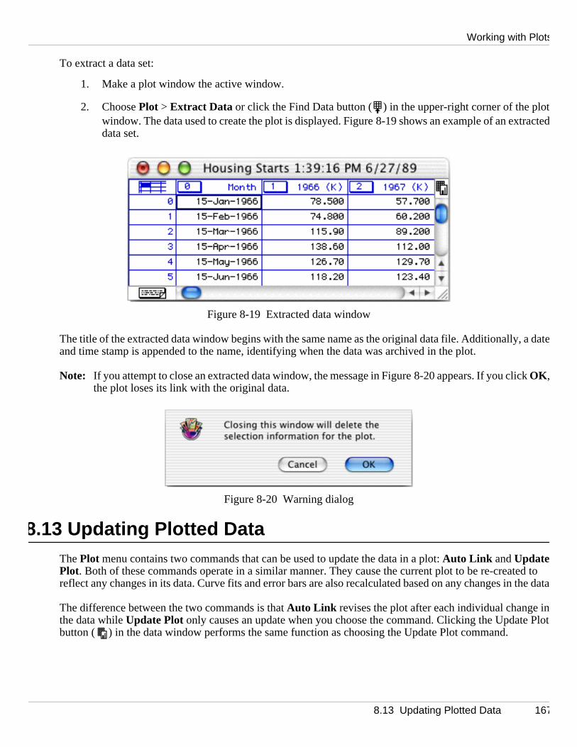
Working with Plots
lotracte
a dat
ck
ted to n the dat
ine Plot
To extract a data set:
1. Make a plot window the active window.
2. Choose Plot > Extract Data or click the Find Data button ( ) in the upper-right corner of the ptwindow. The data used to create the plot is displayed. Figure 8-19 shows an example of an exddata set.
Figure 8-19 Extracted data window
The title of the extracted data window begins with the same name as the original data file. Additionally,eand time stamp is appended to the name, identifying when the data was archived in the plot.
Note: If you attempt to close an extracted data window, the message in Figure 8-20 appears. If you cliOK ,the plot loses its link with the original data.
Figure 8-20 Warning dialog
8.13 Updating Plotted DataThe Plot menu contains two commands that can be used to update the data in a plot: Auto Link and UpdatePlot. Both of these commands operate in a similar manner. They cause the current plot to be re-creareflect any changes in its data. Curve fits and error bars are also recalculated based on any changes ia
The difference between the two commands is that Auto Link revises the plot after each individual change the data while Update Plot only causes an update when you choose the command. Clicking the Updatbutton ( ) in the data window performs the same function as choosing the Update Plot command.
8.13 Updating Plotted Data 167
KaleidaGraph
the data the
th
wn to
th
e
the plo
are fo
th
al plo
These commands are useful if you have a saved plot and need to add or edit points. You can extractfrom the plot (using either the Extract Data command or the Find Data button), modify the data, and useAuto Link or Update Plot commands to revise the plot.
To update plots using the Auto Link command:
1. Open or activate the plot to be updated.
2. Choose Plot > Extract Data or click the Find Data button ( ) to display the data used to createeplot.
3. Turn on Auto Link in the Plot menu.
4. Modify the data and move to another cell. After each data value is modified, the plot is redrashow the changes.
To update plots using the Update Plot command:
1. Open or activate the plot to be updated.
2. Choose Plot > Extract Data or click the Find Data button ( ) to display the data used to createeplot.
3. Make any changes to the extracted data.
4. Choose Plot > Update Plot or click the Update Plot button ( ) in the data window to redraw thplot.
8.14 Plotting Additional DataThere may be times when you want to add additional variables to an existing plot. Instead of creating tfrom scratch, you can open a plot and add new data to it.
Note: If you just want to add a few points to an existing curve, refer to Section 8.13. The steps below radding a new variable to the plot.
To add additional variables to a plot:
1. Open or activate the plot which will have the new data plotted.
2. Choose Plot > Extract Data or click the Find Data button ( ) to display the data used to createeplot.
3. Open the new data or add it to an existing data window.
4. Switch back to the plot and choose Gallery > Template.
5. Select all of the data to be plotted (including the data from the original plot) and click New Plot.
A new plot will be created that includes the additional data. Any curve fits and error bars from the origintwill be applied to the new plot.
168 8.14 Plotting Additional Data

Working with Plots
the
For
, the
8.15 Customizing Bar PlotsThis section explains some of the special features associated with Bar plots. This includes changing spacing between bars, displaying value labels, and creating Line/Column plots.
8.15.1 Changing Bar AttributesThe Plot Extras command (Format menu) contains four options that affect the appearance of the bars.details on changing the fill pattern in the bars, see Section 8.9.3.
To change the attributes of the bars:
1. Choose Format > Plot Extras. The dialog in Figure 8-21 appears.
Figure 8-21 Plot Extras dialog
2. To change the spacing between the bars, edit the Column Offset percentage. Entering a value of 0%removes all space between the bars; a value of 100% displays the bars as spikes.
3. To remove the frame surrounding each bar, clear the Draw Column Frame check box.
4. To make the frame the same color as the fill pattern, clear the Black Column Frame check box.
5. To use a baseline of 1.0 for log scales, select the Adjust Log Baseline check box. Otherwiseminimum axis limit is used for the baseline.
6. Click OK to return to the plot.
8.15 Customizing Bar Plots 169
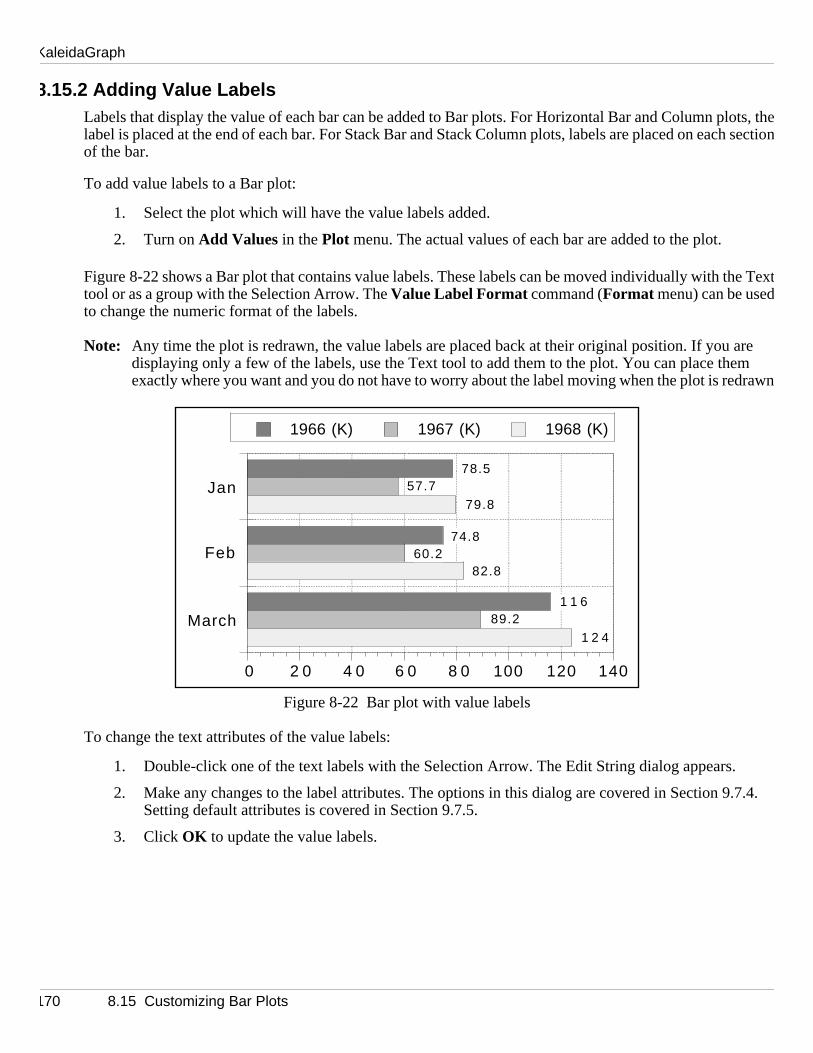
KaleidaGraph
lots, thh sectio
he Tex
re m drawn
.7.4.
8.15.2 Adding Value LabelsLabels that display the value of each bar can be added to Bar plots. For Horizontal Bar and Column pelabel is placed at the end of each bar. For Stack Bar and Stack Column plots, labels are placed on eacnof the bar.
To add value labels to a Bar plot:
1. Select the plot which will have the value labels added.
2. Turn on Add Values in the Plot menu. The actual values of each bar are added to the plot.
Figure 8-22 shows a Bar plot that contains value labels. These labels can be moved individually with tttool or as a group with the Selection Arrow. The Value Label Format command (Format menu) can be usedto change the numeric format of the labels.
Note: Any time the plot is redrawn, the value labels are placed back at their original position. If you adisplaying only a few of the labels, use the Text tool to add them to the plot. You can place theexactly where you want and you do not have to worry about the label moving when the plot is re
Figure 8-22 Bar plot with value labels
To change the text attributes of the value labels:
1. Double-click one of the text labels with the Selection Arrow. The Edit String dialog appears.
2. Make any changes to the label attributes. The options in this dialog are covered in Section 9Setting default attributes is covered in Section 9.7.5.
3. Click OK to update the value labels.
0 2 0 4 0 6 0 8 0 100 120 140
Jan
Feb
March
1966 (K) 1967 (K) 1968 (K)
78.5
74.8
1 1 6
57.7
60.2
89.2
79.8
82.8
1 2 4
170 8.15 Customizing Bar Plots

Working with Plots
e 8-23
line
plot
8.15.3 Adding Lines to Bar and Column PlotsHorizontal Bar and Column plots can have lines added to create Line/Column plots.
To make a Line/Column plot:
1. Create a Horizontal Bar or Column plot, including the variable to be displayed as a line. Figurshows a sample Column plot with two variables plotted.
2. Choose Plot > Plot Style. Use the and buttons to locate the variable to be displayed as a
3. Select a Fill Pattern of Line, as well as the line style, line width, and number of markers to be displayed.
4. Click OK and the plot updates to display a Line/Column plot. Figure 8-24 shows the sample after displaying the second variable as a line.
Figure 8-23 Sample Column plot Figure 8-24 Plot displaying variable as a line
0
4 0
8 0
120
160
Jan March May July
1967 (K) 1968 (K)
0
4 0
8 0
120
160
Jan March May July
1967 (K) 1968 (K)
8.15 Customizing Bar Plots 171

KaleidaGraph
bel
oosin in the
ns for
for
8.16 Customizing Polar PlotsThere are two commands that can be used to change the appearance of Polar plots: Axis Options (Plot menu)and Polar Options (Format menu). Axis Options controls the display of tick marks, grid lines, and axis laswhile Polar Options controls the grid type, reference angle, and direction.
8.16.1 Changing the Display of Tick Marks, Grid Lines, and Axis LabelsThe angular (Ø or X) and the radial (R or Y) axes can be modified using the Axis Options command. ChgPlot > Axis Options displays the dialog in Figure 8-25. The options for each of the axes are discussedfollowing paragraphs.
Figure 8-25 Axis Options dialog
The angular axis is controlled by the X axis settings in the Axis Options dialog. You can use the optioTicks, Grids, and Labels to modify this axis. You can also use the No Axis option to remove the angular axis
The radial axis is controlled by the Y axis settings in the Axis Options dialog. You can use the optionsLimits , Ticks, Grids, and Labels to modify the axis. You can also choose between Linear and Log scaling,or remove the axis with the No Axis option.
172 8.16 Customizing Polar Plots

Working with Plots
pe, dat
8.16.2 Setting the Grid Type, Reference Angle, and DirectionPolar plots have several unique options that control their appearance. These options include the grid tyaformat, reference angle, and direction. All of these options are controlled using the Polar Options command(Format menu).
To change the Polar plot options:
1. Choose Format > Polar Options. The dialog in Figure 8-26 is displayed.
Figure 8-26 Polar Options dialog
2. Make any changes to the settings in this dialog.
3. Click OK to return to the plot.
Figure 8-27 shows a Polar plot displayed in a Clockwise direction, with a circular grid and a 45o Reference Angle. Figure 8-28 shows a Polar plot displayed on a square grid.
Figure 8-27 Polar plot on circular grid Figure 8-28 Polar plot on square grid
0 m32 m34 m36 m38 m3
10 m3
0
3 0
6 0
9 0
120150
180
210
300 330Radius
0 m3
4 m3
4 m3
8 m3
8 m3
0 m3 4 m34 m3 8 m38 m3
Radius
8.16 Customizing Polar Plots 173
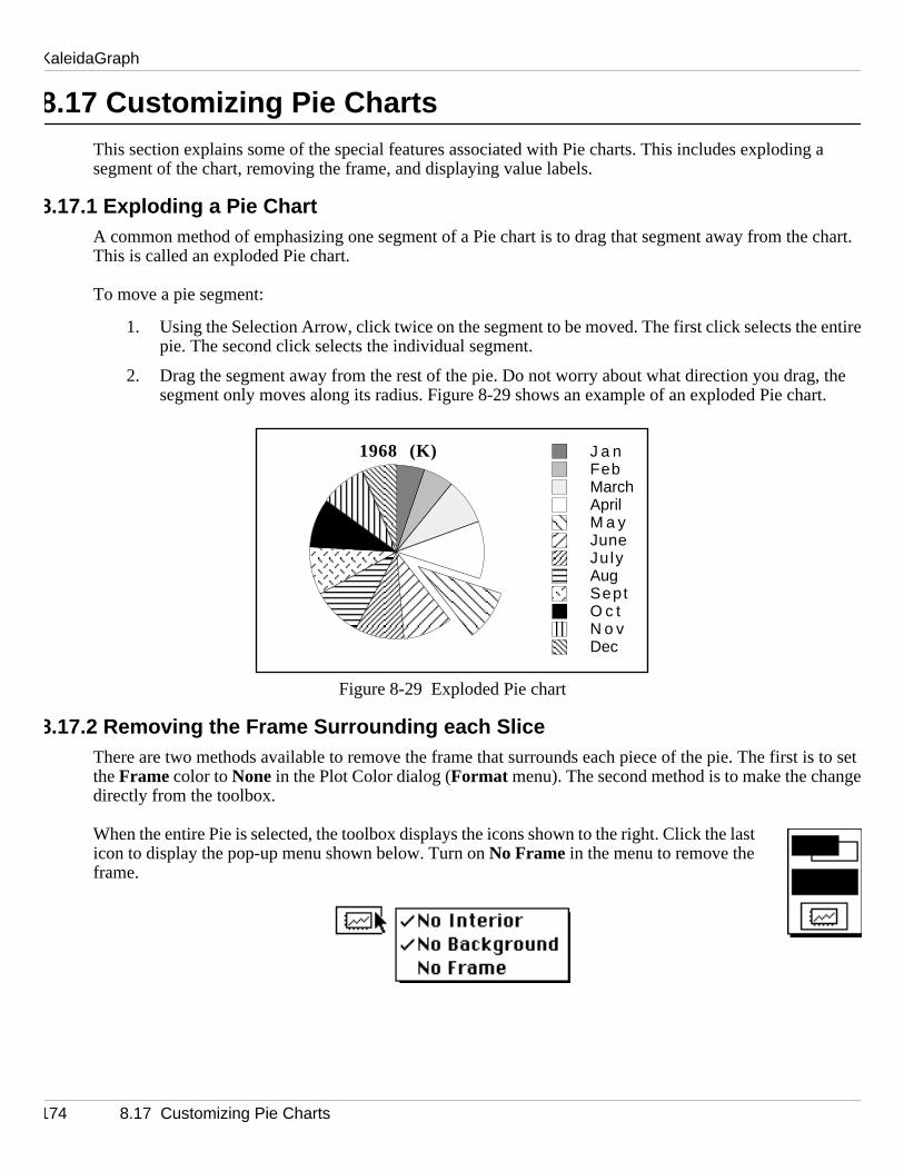
KaleidaGraph
g a
chart.
entir
, the rt.
is to set ge
8.17 Customizing Pie ChartsThis section explains some of the special features associated with Pie charts. This includes explodinsegment of the chart, removing the frame, and displaying value labels.
8.17.1 Exploding a Pie ChartA common method of emphasizing one segment of a Pie chart is to drag that segment away from theThis is called an exploded Pie chart.
To move a pie segment:
1. Using the Selection Arrow, click twice on the segment to be moved. The first click selects theepie. The second click selects the individual segment.
2. Drag the segment away from the rest of the pie. Do not worry about what direction you dragsegment only moves along its radius. Figure 8-29 shows an example of an exploded Pie cha
Figure 8-29 Exploded Pie chart
8.17.2 Removing the Frame Surrounding each SliceThere are two methods available to remove the frame that surrounds each piece of the pie. The first the Frame color to None in the Plot Color dialog (Format menu). The second method is to make the chandirectly from the toolbox.
When the entire Pie is selected, the toolbox displays the icons shown to the right. Click the last icon to display the pop-up menu shown below. Turn on No Frame in the menu to remove the frame.
1968 (K) J a nFebMarchAprilM a yJuneJulyAugSeptO c tN o vDec
174 8.17 Customizing Pie Charts

Working with Plots
plot.
he Tex
re m
awn.
.7.4.
8.17.3 Adding Value LabelsLabels that display the percentage of each slice relative to the entire pie can be added to Pie charts.
To add value labels to a Pie chart:
1. Select the Pie chart which will have the value labels added.
2. Turn on Add Values in the Plot menu. The percentage values of each pie slice are added to theTo display the actual values, select the Display Pie Values check box in the Plot Extras dialog (Format menu).
Figure 8-30 shows a Pie chart that contains value labels. These labels can be moved individually with tttool or as a group with the Selection Arrow. The Value Label Format command (Format menu) can be usedto change the numeric format of the labels.
Note: Any time the plot is redrawn, the value labels are placed back at their original position. If you adisplaying only a few of the labels, use the Text tool to add them to the plot. You can place theexactly where you want and do not have to worry about the label moving when the plot is redr
Figure 8-30 Pie chart with value labels
To change the attributes of the value labels:
1. Double-click one of the text labels with the Selection Arrow. The Edit String dialog appears.
2. Make any changes to the label attributes. The options in this dialog are covered in Section 9Setting default attributes is covered in Section 9.7.5.
3. Click OK to update the value labels.
J a nFebMarchAprilM a yJuneJulyAugSeptO c tN o vDec
5.38%5.58%
8.35%
10.7%
9.37%
9.17%9.26%
9.07%
8.92%
9.31%
8.43%6.44%
8.17 Customizing Pie Charts 175

KaleidaGraph
176 8.17 Customizing Pie Charts
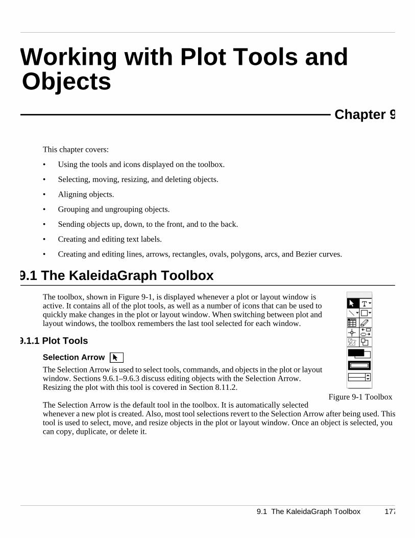
Working with Plot Tools and Objects
Chapter 9
d. Thid, you
This chapter covers:
• Using the tools and icons displayed on the toolbox.
• Selecting, moving, resizing, and deleting objects.
• Aligning objects.
• Grouping and ungrouping objects.
• Sending objects up, down, to the front, and to the back.
• Creating and editing text labels.
• Creating and editing lines, arrows, rectangles, ovals, polygons, arcs, and Bezier curves.
9.1 The KaleidaGraph ToolboxThe toolbox, shown in Figure 9-1, is displayed whenever a plot or layout window is active. It contains all of the plot tools, as well as a number of icons that can be used to quickly make changes in the plot or layout window. When switching between plot and layout windows, the toolbox remembers the last tool selected for each window.
9.1.1 Plot Tools
Selection Arrow
The Selection Arrow is used to select tools, commands, and objects in the plot or layout window. Sections 9.6.1–9.6.3 discuss editing objects with the Selection Arrow. Resizing the plot with this tool is covered in Section 8.11.2.
The Selection Arrow is the default tool in the toolbox. It is automatically selectedwhenever a new plot is created. Also, most tool selections revert to the Selection Arrow after being usestool is used to select, move, and resize objects in the plot or layout window. Once an object is selectecan copy, duplicate, or delete it.
Figure 9-1 Toolbox
9.1 The KaleidaGraph Toolbox 177

KaleidaGraph
splay 9.7.
ys a ssed in
his pes is
.
corners
8.3.
Text Tool
This tool is used to add and modify plot labels. Clicking this tool and holding down the mouse button disa pop-up menu that can be used to edit selected text labels. Using the Text tool is covered in Section
Line/Arrow Tool
This tool is used to draw lines or arrows. Clicking this tool and holding down the mouse button displapop-up menu that contains the lines and arrows that can be drawn. Creating lines and arrows is discuSection 9.8.1.
Object ToolClicking the object tool (to the right of the Line/Arrow tool) displays the pop-up menu shown below. Tmenu contains six drawing tools that can be used to create various shapes. Creating and editing shacovered in Section 9.8.
Box Tool
This tool is used to draw square and rectangular boxes. Creating boxes is discussed in Section 9.8.2
Rounded Rectangle Tool
This tool is used to draw squares and rectangles with rounded corners. Creating rectangles with roundis discussed in Section 9.8.2.
Oval Tool
This tool is used to draw ovals and circles. Creating ovals and circles is discussed in Section 9.8.2.
Polygon Tool
This tool is used to draw polygons (multi-sided objects). Creating polygons is discussed in Section 9.
Arc Tool
This tool is used to create arcs. Creating arcs is discussed in Section 9.8.2.
Bezier Curve Tool
This tool is used to draw Bezier curves. Creating Bezier curves is covered in Section 9.8.4.
Table Tool
This tool is used to create tables of data. The use of this tool is covered in Section 9.2.
178 9.1 The KaleidaGraph Toolbox
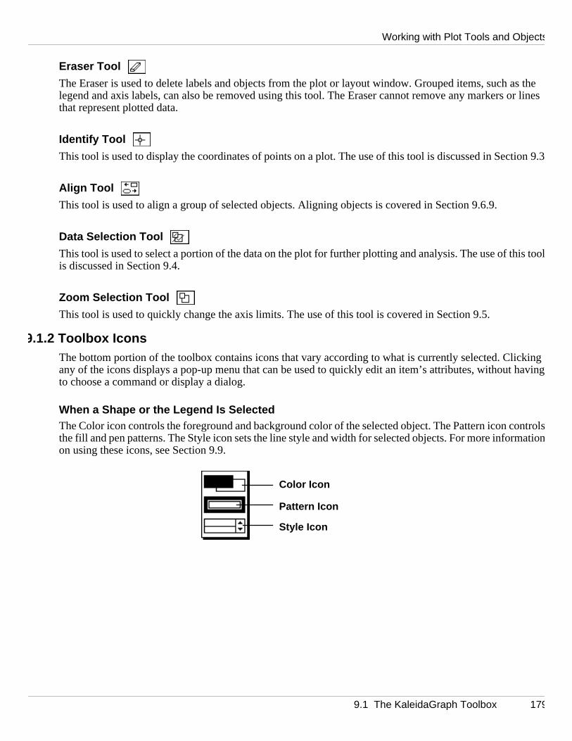
Working with Plot Tools and Objects
as the or lines
tion 9.3
his too
cking having
ontrolrmatio
Eraser Tool
The Eraser is used to delete labels and objects from the plot or layout window. Grouped items, such legend and axis labels, can also be removed using this tool. The Eraser cannot remove any markersthat represent plotted data.
Identify Tool
This tool is used to display the coordinates of points on a plot. The use of this tool is discussed in Sec
Align Tool
This tool is used to align a group of selected objects. Aligning objects is covered in Section 9.6.9.
Data Selection Tool
This tool is used to select a portion of the data on the plot for further plotting and analysis. The use of tlis discussed in Section 9.4.
Zoom Selection Tool
This tool is used to quickly change the axis limits. The use of this tool is covered in Section 9.5.
9.1.2 Toolbox IconsThe bottom portion of the toolbox contains icons that vary according to what is currently selected. Cliany of the icons displays a pop-up menu that can be used to quickly edit an item’s attributes, withoutto choose a command or display a dialog.
When a Shape or the Legend Is SelectedThe Color icon controls the foreground and background color of the selected object. The Pattern icon csthe fill and pen patterns. The Style icon sets the line style and width for selected objects. For more infonon using these icons, see Section 9.9.
Color Icon
Pattern Icon
Style Icon
9.1 The KaleidaGraph Toolbox 179

KaleidaGraph
ou to C.4.
u to ling, ticn alsred in
able played.h. Fo
When the Plot Frame Is SelectedThe Color icon controls the interior and background colors for the plot. The Transparent icon allows yleave the interior or background transparent. For more information on using these icons, see Section
When an Axis Is SelectedThe Color icon determines the frame and grid colors. The first of the two Axis Options icons allows yohide the selected axis or exchange the X and Y axes. The second Axis Options icon controls axis scakmark display, grid line display, and the format of the axis labels. If the X2 or Y2 axis is selected, you caolink the axes. The interior of the icon displays which axis is currently selected. The Color icon is coveSection C.4; the Axis Options icons are covered in Section C.2.
When a Marker Is Selected in the LegendThe Variable Color icon controls the color of the variable. The two icons in the middle control the varimarkers and fill patterns. The Marker icon determines the marker type, size, and number of markers disThe Fill Pattern icon controls the fill pattern. The Style icon determines the variable’s line style and widtrmore information on using these icons, see Section C.3.
Color Icon
No Color Icon
Color Icon
Axis Options Icons
Variable Color Icon
Style Icon
Fill Pattern IconMarker Icon
180 9.1 The KaleidaGraph Toolbox
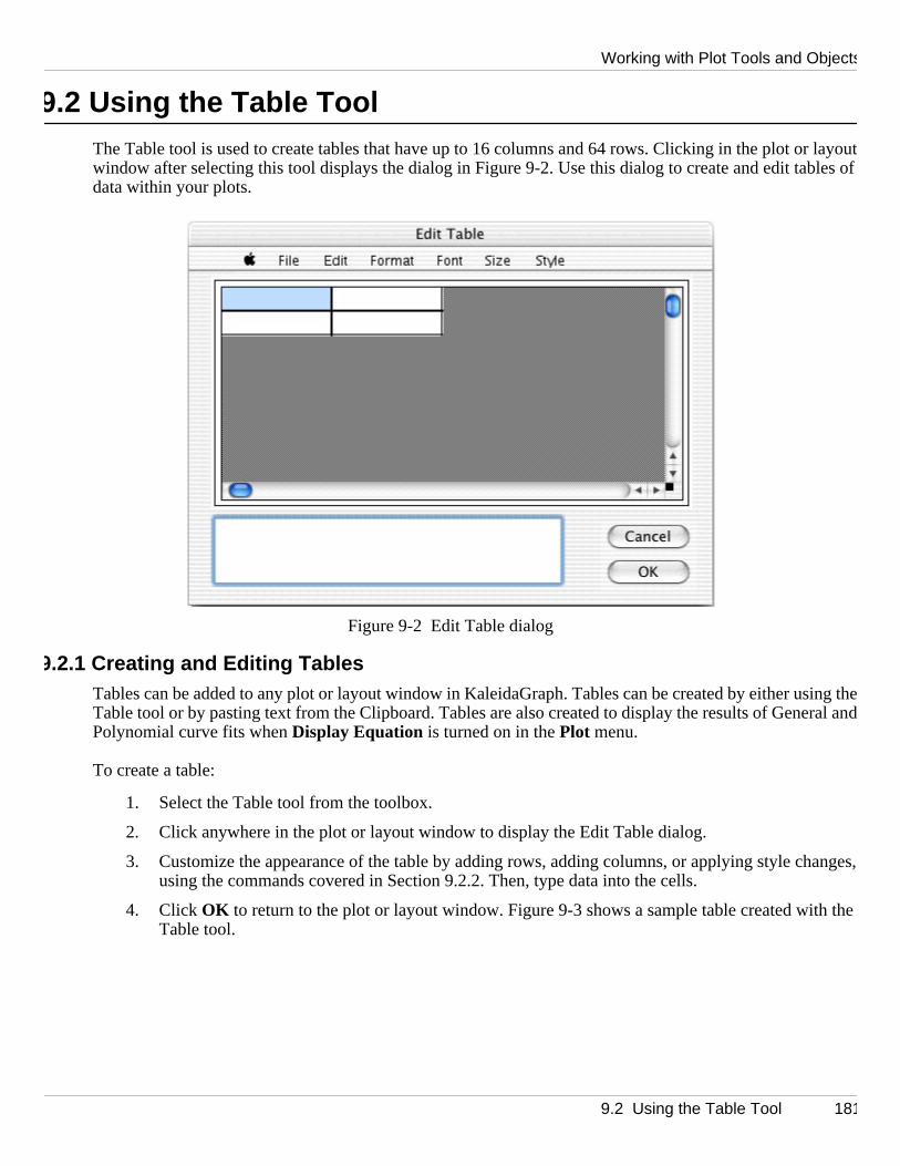
Working with Plot Tools and Objects
r layoules of
sing thral an
anges,
the
9.2 Using the Table ToolThe Table tool is used to create tables that have up to 16 columns and 64 rows. Clicking in the plot otwindow after selecting this tool displays the dialog in Figure 9-2. Use this dialog to create and edit tabdata within your plots.
Figure 9-2 Edit Table dialog
9.2.1 Creating and Editing TablesTables can be added to any plot or layout window in KaleidaGraph. Tables can be created by either ueTable tool or by pasting text from the Clipboard. Tables are also created to display the results of GenedPolynomial curve fits when Display Equation is turned on in the Plot menu.
To create a table:
1. Select the Table tool from the toolbox.
2. Click anywhere in the plot or layout window to display the Edit Table dialog.
3. Customize the appearance of the table by adding rows, adding columns, or applying style chusing the commands covered in Section 9.2.2. Then, type data into the cells.
4. Click OK to return to the plot or layout window. Figure 9-3 shows a sample table created withTable tool.
9.2 Using the Table Tool 181

KaleidaGraph
e
next
on
oard.
if any
ssary,t cell.
ilar to
Figure 9-3 Sample tableTo edit a table:
1. Double-click the table with the Selection Arrow. The Edit Table dialog appears, displaying thcontents of the table.
2. Make the necessary changes to the table, using the commands covered in Section 9.2.2.
3. Click OK to return to the plot or layout window.
9.2.2 Table Tool CommandsFile Menu
• New - This command deletes any existing cells and creates a new table.
• Open - This command loads a text file into the table. A tab in the text forces the data into thecell. A return in the text forces the data into the next row of the table.
• Set Defaults - This command saves the current table settings as the default. For information setting the defaults, see Section 9.2.3.
• Close - This command closes the dialog. Clicking OK performs the same function.
Edit Menu
• Cut - This command deletes the contents of the selected cells and places them on the Clipb
• Copy - This command copies the selection to the Clipboard, replacing the previous contents,
• Paste - This command places the Clipboard’s contents into the selected cell positions. If necethis command adds cells to the table. A tab in the text forces the data following it into the nexA return in the text causes the data following it into the next row of the table.
• Clear - This command deletes the contents of the selected cells. This command operates simCut, except that the contents of the Clipboard are not disturbed.
Statistics for the Example #1 data setTest #3Test #2Test #1
2.050.550000010.5Minimum
7.69999986.19999986.8000002Maximum
96.5759.0787.43Sum
252525Points
3.86282.36283.4972Mean
3.34000021.843.5Median
4.1922612.86995683.9020287RMS
1.66264981.66264981.7664171Std Deviation
2.76440432.76440433.1202294Variance
0.332529960.332529960.35328342Std Error
0.842622080.84262208-0.013367556Skewness
-0.40279496-0.402795-1.1877315Kurtosis
182 9.2 Using the Table Tool

Working with Plot Tools and Objects
othe
ly table
using
nts
any
any
cells.he
f you
• Copy Table - This command copies the table to the Clipboard as an image, for inclusion in anrprogram.
• Copy Style - This command copies the style of the current selection. This allows you to quickapply a particular style to sections of the table. If necessary, this command adds cells to the when the style is pasted.
• Select All - This command selects the entire contents of the table.
• Insert Rows - This command inserts a row above the current selection.
• Insert Columns - This command inserts a column to the left of the current selection.
• Delete Rows - This command deletes any selected rows. The entire row is deleted using this command.
• Delete Columns - This command deletes any selected columns. The entire column is deletedthis command.
Format Menu
• Left, Right, or Center Justification - These commands control the alignment of the cell’s conte
• Cell Horizontal Line - This command sets the line width and color of the line on the bottom ofselected cells.
• Cell Vertical Line - This command sets the line width and color of the line on the right side ofselected cells.
Note: If None is selected for the line width, a vertical line is not displayed between adjacent The cells are treated as a single unit. Type the string in the leftmost cell and choose tjustification. The contents appear across all cells in the unit. This technique is used togenerate labels that span multiple cells.
• Cell Background - This command sets a background pattern and color within selected cells. Iwant a solid color, choose 100% Fill.
• Frame Style - This command sets the style of the table’s frame.
• Frame Color - This command sets the color of the table’s frame.
9.2 Using the Table Tool 183

KaleidaGraph
e
it
ste
menuecond
listed f th
entir in thate font
• Options - This command displays the dialog in Figure 9-4.
Figure 9-4 Format Options dialog
- Minimum Row Size, Minimum Column Size - The values entered in these fields determinthe minimum row height and column width (one pixel equals 1/72 inch).
- Pack Rows, Pack Columns - Packing minimizes the white space within cells (horizontally whPack Rows and vertically with Pack Columns).
- Fixed Row Height, Fixed Column Width - These options control how much white space exiswithin cells. When these check boxes are selected, the row or column sizes are the samthroughout the table.
Font MenuThe Font menu contains all of the fonts that are currently installed. Choosing a different font from this changes the font for the entire cell, even if only a portion of the cell is selected. If you need to use a sfont in the cell, use the Alt. Font command in the Style menu.
Size MenuThis menu contains the sizes that are available for displaying fonts. You can specify a size that is notusing the Other command in this menu. The font size is applied to the entire cell, even if only a portion oecell is selected.
Style MenuThe Style menu is divided into three sections. The commands in the first section control the style of theecell, even if only a portion of the cell is selected. The color of the text is controlled using the commandesecond section. The commands in the third section allow you to display selected characters in an altern,as subscripts, or as superscripts. The Normal, Superscript, Subscript, and Alt. Font commands are the onlycommands in the Edit Table dialog that have an affect on selected portions of a cell.
184 9.2 Using the Table Tool

Working with Plot Tools and Objects
set th
ble.
g
xcep
ce the
indow
nate
t ional
9.2.3 Setting Defaults for TablesThe Edit Table dialog initially displays four cells. In addition to being part of the table, they are used to edefault layout for generating new tables. They control the layout as follows:
• cell 1 (upper left): This cell controls itself and does not affect the defaults for the rest of the ta
• cell 2 (upper right): This cell controls the default settings for the top row of the table (excludincell 1).
• cell 3 (lower left): This cell controls the default settings for column one of the table (excludingcell 1).
• cell 4 (lower right): This cell controls the default settings for the body of the table (everything etrow one and column one).
Change the attributes (font, size, style, justification, and so on) in each of the four cells. Then, chooseFile > Set Defaults to remember the settings. Your default settings are saved as part of the Style file.
9.3 Using the Identify ToolUse the Identify tool to find the coordinates of any point in the plot window. It can also be used to placoordinates directly on the plot or the Clipboard.
To use the Identify tool:
1. Select the Identify tool from the toolbox.
2. Click anywhere in the plot. The coordinates are displayed in the upper-left corner of the plot w
3. To leave the coordinates on the plot, press Alt (Windows) or Option (Macintosh) when releasing themouse button. A tag is placed at the current location. The appearance of the X and Y coordilabels is based on the current settings in the X and Y Label Format dialogs (Format menu), with theexception of adding one extra digit of accuracy.
4. To place the coordinates on the Clipboard, press Shift when releasing the mouse button. The firstime you do this, the Clipboard is cleared and the first set of coordinates is copied. Any additcoordinates are appended to the information already stored on the Clipboard.
9.3 Using the Identify Tool 185

KaleidaGraph
This is
Datallows
k the
ve
can
x.
show
9.4 Using the Data Selection ToolUse the Data Selection tool to select a portion of the displayed data for further plotting and analysis. accomplished by enclosing a region of the plot in a polygon.
This tool is particularly useful for eliminating outliers from a plot during a regression analysis. After theaSelection tool is used, all curve fits are automatically recalculated based on the remaining data. This arbitrary data points to be removed from a plot in a very selective, graphical manner.
To enclose the data points in a polygon:
1. Select the Data Selection tool from the toolbox.
2. Position the crosshair at the point where you want to begin forming line segments. Then, clicmouse button to begin. A small square marks the starting point.
3. Move the mouse to the point where you want the first segment of the polygon to end.
Note: Pressing Alt (Windows) or Option (Macintosh) when creating the polygon removes the points that lie within it. This feature enables you to select the points you want to remoinstead of the points you want to keep.
4. Move the mouse and click again to create the second segment.
5. Continue moving and clicking the mouse until the desired data is enclosed in a polygon. Youcomplete the polygon by clicking the hollow square, double-clicking the mouse, pressing Enter (Windows) or Return (Macintosh), or clicking when the crosshair is positioned over the toolboFigure 9-5 shows a sample plot that has a region of data selected.
Figure 9-5 Using the Data Selection tool
The plot is then redrawn and only the points that lie within the polygon (or outside when using the Alt or Option key) are replotted. The points that are removed become masked in the data window. Figure 9-6sthe plot after being redrawn to only include the points within the polygon.
186 9.4 Using the Data Selection Tool

Working with Plot Tools and Objects
urn to
m box,n the
new Y2 ws
Figure 9-6 Resulting plot after using the Data Selection tool
Note: Any polygon bounding a selection region can have a maximum of 100 bounding points. To retthe original plot and unmask the data, double-click the Data Selection tool.
9.5 Using the Zoom Selection ToolUse the Zoom Selection tool to quickly change the axis limits. This is accomplished by creating a zoowhich defines the new limits for the plot. This tool produces an effect similar to specifying axis limits iAxis Options dialog (Plot menu).
To use the Zoom Selection tool:
1. Select the Zoom Selection tool from the toolbox.
2. Drag over a region of the graph. The upper-left and lower-right corners of the box define thelimits for the plot. For Double Y, Double X, and Double XY plots, you can rescale the X2 andaxes by pressing Ctrl (Windows) or (Macintosh) when creating the zoom box. Figure 9-7 shoa sample plot with new limits being selected.
0
1
2
3
4
5
6
0 2 4 6 8 1 0 1 2 1 4
Test #1
y = 5.4066 + -0.32318x R= 0.84924
Ra
ng
e
Time
9.5 Using the Zoom Selection Tool 187
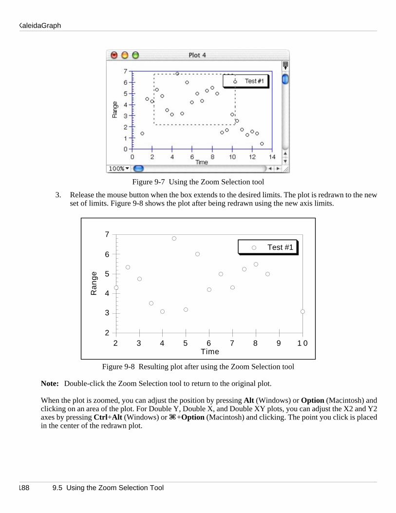
KaleidaGraph
the ne
nd Y2
Figure 9-7 Using the Zoom Selection tool
3. Release the mouse button when the box extends to the desired limits. The plot is redrawn to wset of limits. Figure 9-8 shows the plot after being redrawn using the new axis limits.
Figure 9-8 Resulting plot after using the Zoom Selection tool
Note: Double-click the Zoom Selection tool to return to the original plot.
When the plot is zoomed, you can adjust the position by pressing Alt (Windows) or Option (Macintosh) andclicking on an area of the plot. For Double Y, Double X, and Double XY plots, you can adjust the X2 aaxes by pressing Ctrl +Alt (Windows) or +Option (Macintosh) and clicking. The point you click is placedin the center of the redrawn plot.
2
3
4
5
6
7
2 3 4 5 6 7 8 9 1 0
Test #1
Ra
ng
e
Time
188 9.5 Using the Zoom Selection Tool

Working with Plot Tools and Objects
d click.
n
shows
, if you
legend
tline o
xample
9.6 Working with Objects
9.6.1 Selecting and Deselecting ObjectsTo modify an object, it must first be selected. To select an object, position the pointer over the object anObject handles appear around the object.
There are three methods for selecting multiple objects:
• Press Shift and use the Selection Arrow to click the objects one at a time. Figure 9-9 shows aexample of selecting objects one at a time.
• Use the Selection Arrow to drag a dotted box around the objects to be selected. Figure 9-10objects being selected in this manner.
• Choose Edit > Select All to select all of the objects.
Note: When multiple objects are selected, changes affect each of the selected objects. For examplechange the fill pattern, it changes in all of the selected objects.
To deselect objects:
• To deselect all selected objects, click a blank portion of the window or press Esc.
• To deselect objects one at a time, press Shift while clicking the object. The object you click is deselected. All other objects remain selected.
9.6.2 Moving ObjectsAfter objects are created in the plot or layout window, it may be necessary to reposition them. The plot, ,and any text labels can also be moved using the method described below.
To move objects:
1. Select the object to be moved.
2. Position the pointer over the selected object and drag it to a new position. As you drag, an oufthe object is displayed. If you drag to the edge of the window, the window scrolls.
3. Release the mouse button when the object is in the desired location. Figure 9-11 shows an eof an object being moved.
Figure 9-9 Clicking objects individually Figure 9-10 Dragging the Selection Arrow
9.6 Working with Objects 189

KaleidaGraph
keys
hapes
object
ircle.
ct
Figure 9-11 Moving an object
Note: You can also move selected objects vertically or horizontally using the arrow keys. If the arroware used, the objects move one pixel in the specified direction (10 pixels if you press Shift at the sametime).
9.6.3 Resizing ObjectsAny object can be resized in the plot or layout window. This includes the plot axes, legend, and any screated with the drawing tools.
Note: The legend cannot be resized if it only contains a single item.
To resize an object:
1. Select the object to be resized.
2. Drag any one of the handles until the object reaches the desired size. Figure 9-12 shows anbeing resized.
Figure 9-12 Resizing an object
Note: To resize the object proportionally about its center, press Alt (Windows) or Option (Macintosh) whendragging the handle. By pressing Shift as you drag, you can constrain the shape to a square or c
9.6.4 Duplicating ObjectsTo duplicate an object:
1. Select the object to be duplicated.
2. Choose Edit > Duplicate. A copy of the object is placed slightly below and to the right of the original. Its handles are visible to indicate that it is selected. An example of a duplicated objeappears in Figure 9-13.
190 9.6 Working with Objects
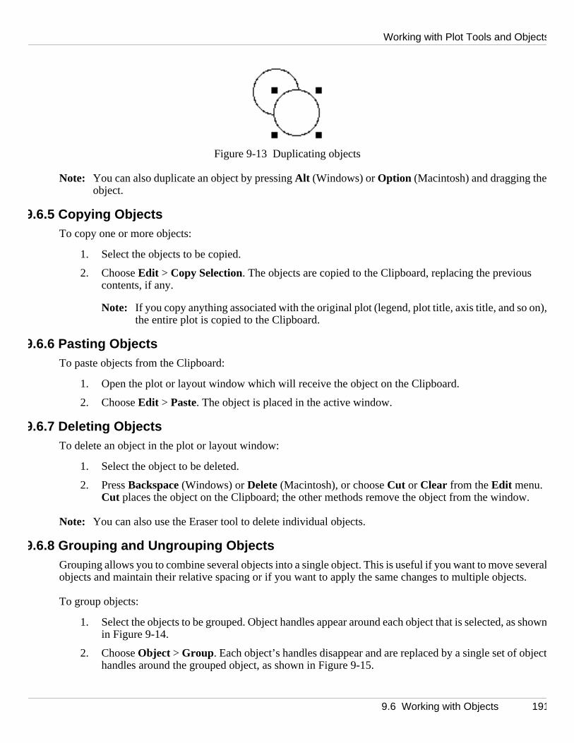
Working with Plot Tools and Objects
on),
w.
everats.
as show
bjec
Figure 9-13 Duplicating objects
Note: You can also duplicate an object by pressing Alt (Windows) or Option (Macintosh) and dragging theobject.
9.6.5 Copying ObjectsTo copy one or more objects:
1. Select the objects to be copied.
2. Choose Edit > Copy Selection. The objects are copied to the Clipboard, replacing the previouscontents, if any.
Note: If you copy anything associated with the original plot (legend, plot title, axis title, and sothe entire plot is copied to the Clipboard.
9.6.6 Pasting ObjectsTo paste objects from the Clipboard:
1. Open the plot or layout window which will receive the object on the Clipboard.
2. Choose Edit > Paste. The object is placed in the active window.
9.6.7 Deleting ObjectsTo delete an object in the plot or layout window:
1. Select the object to be deleted.
2. Press Backspace (Windows) or Delete (Macintosh), or choose Cut or Clear from the Edit menu. Cut places the object on the Clipboard; the other methods remove the object from the windo
Note: You can also use the Eraser tool to delete individual objects.
9.6.8 Grouping and Ungrouping ObjectsGrouping allows you to combine several objects into a single object. This is useful if you want to move slobjects and maintain their relative spacing or if you want to apply the same changes to multiple objec
To group objects:
1. Select the objects to be grouped. Object handles appear around each object that is selected, nin Figure 9-14.
2. Choose Object > Group. Each object’s handles disappear and are replaced by a single set of othandles around the grouped object, as shown in Figure 9-15.
9.6 Working with Objects 191

KaleidaGraph
The
type o
long wit
s.
re 9-18
Once you have grouped objects together, you can no longer select or modify the objects individually.UnGroup command can be used to separate a grouped object into its original components.
To ungroup an object:
1. Select the object to be ungrouped.
2. Choose Object > UnGroup. Object handles appear for each individual object.
9.6.9 Aligning ObjectsKaleidaGraph has two ways to align objects: the Align tool from the toolbox and the Align command (Objectmenu). Selecting either displays the pop-up menu in Figure 9-16. The icons in this menu indicate thefalignment applied to the objects.
Figure 9-16 Alignment pop-up menu
To align objects:
1. Select the objects to be aligned. Figure 9-17 shows some sample objects that are selected, aha reference line.
2. Choose Object > Align or select the Align tool from the toolbox to display the alignment option
3. Select one of the icons from the menu. The objects are aligned based on your selection. Figushows the objects after aligning them by their left edges.
Figure 9-14 Before grouping Figure 9-15 After grouping
192 9.6 Working with Objects

Working with Plot Tools and Objects
objec difficul
ts
he
9.6.10 Sending Objects Up or DownEach time you create an object in the plot or layout window, it is placed on top of all other objects in thetstacking order. This order is important because objects near the bottom of the stack may be hidden ortto modify.
There are four commands in the Object menu that enable you to change the ordering of objects. These commands are: Up, Bring To Front , Down, and Send To Back. These commands are useful when objecoverlap in a plot or layout.
To change the ordering of an object:
1. Select the object to be modified.
2. Choose the appropriate command from the Object menu. The selected object is repositioned in twindow.
• Up - Moves the selected object forward one level in the object order.
• Bring To Front - Moves the selected object in front of all other objects.
• Down - Moves the selected object backward one level in the object order.
• Send To Back - Moves the selected object behind all other objects.
Figure 9-17 Objects before being aligned Figure 9-18 Objects after being aligned
9.6 Working with Objects 193

KaleidaGraph
low it
Figure 9-19 shows five stacked objects with the middle object (the oval) selected. The four figures beshow how the original objects appear after choosing each of the four commands.Figure 9-19 Original set of objects
After choosing Up After choosing Bring To Front
After choosing Down After choosing Send To Back
194 9.6 Working with Objects
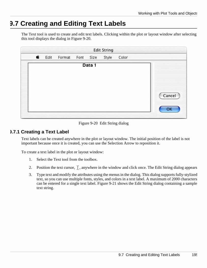
Working with Plot Tools and Objects
cting
t
pears
ylizeactersample
9.7 Creating and Editing Text LabelsThe Text tool is used to create and edit text labels. Clicking within the plot or layout window after selethis tool displays the dialog in Figure 9-20.
Figure 9-20 Edit String dialog
9.7.1 Creating a Text LabelText labels can be created anywhere in the plot or layout window. The initial position of the label is noimportant because once it is created, you can use the Selection Arrow to reposition it.
To create a text label in the plot or layout window:
1. Select the Text tool from the toolbox.
2. Position the text cursor, , anywhere in the window and click once. The Edit String dialog ap
3. Type text and modify the attributes using the menus in the dialog. This dialog supports fully-stdtext, so you can use multiple fonts, styles, and colors in a text label. A maximum of 2000 charcan be entered for a single text label. Figure 9-21 shows the Edit String dialog containing a stext string.
9.7 Creating and Editing Text Labels 195

KaleidaGraph
dialog.
lishe
. Th
els
Figure 9-21 Sample string in the Edit String dialog
4. Click OK to return to the plot or layout window.
9.7.2 Editing Plot LabelsLegend TextThe legend text can be edited using the Text tool. Double-clicking a text label displays the Edit String Change the legend text as needed and click OK to return to the plot.
It is also possible to move items in the legend to different locations using the Text tool. This is accompdby dragging a label to a new position with the Text tool.
Plot and Axis TitlesPlot and axis titles can be edited by double-clicking them with either the Text tool or the Selection ArroweEdit String dialog appears, containing the current text string. Change the text as needed and click OK to returnto the plot.
Value and Axis LabelsValue and axis labels are unique because they can be edited individually or as a group.
To edit value or axis labels individually:
1. Select the Text tool from the toolbox.
2. Double-click the label to be modified. The label appears in the Edit String dialog.
3. Change the label text and formatting.
4. Click OK to return to the plot.
Note: Be careful when editing value and axis labels in this manner. If the plot is redrawn, the labrevert to their original state.
196 9.7 Creating and Editing Text Labels
Working with Plot Tools and Objects
labe
the neede
eat
aGrap
e plot,
hes
if any
To edit value or axis labels as a group:
1. Select the Selection Arrow from the toolbox.
2. Double-click one of the labels in the group. The label appears in the Edit String dialog, but theltext cannot be edited because the labels are selected as a group.
3. Make the necessary formatting changes to the label.
4. Click OK to return to the plot. The entire group is redrawn to reflect the changes.
Individual Text LabelsAny text label created with the Text tool can be edited by double-clicking it with either the Text tool orSelection Arrow. The Edit String dialog appears, containing the current text string. Change the text asdand click OK to return to the plot.
9.7.3 Adding Subscripts or Superscripts to a Text LabelTo add subscripts or superscripts to a label:
1. Using the Text tool, double-click an existing label or click within the plot or layout window to crea new label.
2. Select the text to be converted.
3. Choose Subscript or Superscript from the Style menu.
4. Click OK .
Note: The Edit String dialog does not display characters as subscripts or superscripts. Instead, Kaleidhinserts either \d (subscript) or \u (superscript) before the characters and \n (normal) after the characters.These extra characters are only displayed in the Edit String dialog. As soon as you return to ththe subscripts or superscripts are displayed correctly.
The Text Options dialog (Format menu) contains four settings (Superscript Offset, Subscript Offset, Sub/Super Size, and Only use built-in sizes) that affect the appearance of subscripts and superscripts. Tesettings can be modified to control the offset and size of these characters.
9.7.4 Text Tool CommandsEdit Menu
• Cut - This command removes the selection and places it on the Clipboard.
• Copy - This command copies the selection to the Clipboard, replacing the previous contents,
• Paste - This command places the contents of the Clipboard at the insertion point.
• Clear - This command deletes the selection. This command operates similar to Cut, except that thecontents of the Clipboard are not disturbed.
• Select All - This command selects all of the text in the dialog.
9.7 Creating and Editing Text Labels 197

KaleidaGraph
lot o
fou unti
d.
in the
listed sing
laying
in the
and have
Format Menu
• Left, Right, or Center Justification - The justification of text labels can be set to either Left , Right,or Center. This setting determines the label placement in relation to where you clicked in the prlayout window with the Text tool.
• 0, 90, 180, and 270o Rotation - These commands set the orientation of the text label to one of rpositions, moving counter-clockwise from horizontal. You will not see any changes to the textlyou return to the plot or layout window.
• Erase Background - When this command is turned on, anything behind the text label is erase
Font MenuThe Font menu contains all of the fonts that are currently installed. It is possible to use multiple fonts same text label by choosing a different font for selected portions of the label.
Size MenuThis menu contains the sizes that are available for displaying fonts. You can specify a size that is notusing the Other command in this menu. Multiple font sizes can be used in the same text label by chooadifferent font size for selected portions of the label.
Style MenuThis menu lists the different styles that can be applied to the text. It also includes commands for dispcharacters as subscripts or superscripts.
Color MenuThis menu displays the current color choices available for the text label. Multiple colors can be used same text label by choosing a different color for selected portions of the label.
9.7.5 Setting Defaults for Text LabelsYou can set defaults for a number of different text labels in the Text Options dialog (Format menu). The attributes that you select are saved as part of the Style file. This enables you to set your preferences KaleidaGraph remember them the next time you start the program.
To set defaults for text labels:
1. Choose Format > Text Options to display the dialog in Figure 9-22.
198 9.7 Creating and Editing Text Labels
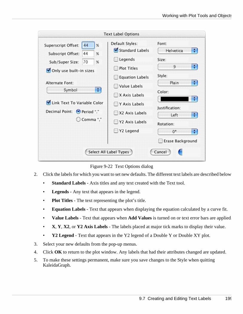
Working with Plot Tools and Objects
below
fit.
d
ed.
Figure 9-22 Text Options dialog
2. Click the labels for which you want to set new defaults. The different text labels are described
• Standard Labels - Axis titles and any text created with the Text tool.
• Legends - Any text that appears in the legend.
• Plot Titles - The text representing the plot’s title.
• Equation Labels - Text that appears when displaying the equation calculated by a curve
• Value Labels - Text that appears when Add Values is turned on or text error bars are applie.
• X, Y, X2, or Y2 Axis Labels - The labels placed at major tick marks to display their value.
• Y2 Legend - Text that appears in the Y2 legend of a Double Y or Double XY plot.
3. Select your new defaults from the pop-up menus.
4. Click OK to return to the plot window. Any labels that had their attributes changed are updat
5. To make these settings permanent, make sure you save changes to the Style when quitting KaleidaGraph.
9.7 Creating and Editing Text Labels 199

KaleidaGraph
es in the bject’s
9.8 Creating and Editing ShapesYou can create lines, arrows, rectangles, rounded rectangles, ovals, polygons, arcs, and Bezier curvplot or layout window. Once a shape is created, you can use the icons in the toolbox to change the oattributes. This topic is covered in Section 9.9.
9.8.1 Lines and ArrowsTo create a line or arrow:
1. Click the Line tool on the toolbox.
2. Click the Line tool again and hold down the mouse button to display the pop-up menu in Figure 9-23. Choose the first item in this menu to draw a line or select the type of arrow you want to create.
3. Position the crosshair at the point where you want to begin drawing the line. When creating an arrow, the arrowhead is placed at this position.
4. Drag to draw the line. By pressing Shift as you drag, you can constrain the line to rotate in 45o increments.
5. Release the mouse button when the line is the desired length. The line appears with object handles to indicate that it is selected.
Figure 9-24 Drawing a line
Figure 9-23 Line tool menu
200 9.8 Creating and Editing Shapes

Working with Plot Tools and Objects
ne.
ou can
nt it.
to a
appear
To edit a line or arrow:
1. Select the line or arrow with the Selection Arrow. Object handles appear at the ends of the li
2. Position the pointer over one of the handles.
3. Drag the handle to adjust the length or angle of the line.
4. You can change the arrowhead type by selecting a different arrow from the pop-up menu. Yswitch the ends of the arrow by choosing Reverse from the menu.
5. When you are finished, click away from the line to deselect it.
To edit an arrowhead:
1. Double-click the arrow (or click once and choose Object > Edit Object) to display the dialog in Figure 9-25.
Figure 9-25 Arrow Head dialog
2. Edit the values in the dialog until the arrowhead in the preview window looks the way you wa
3. Click OK to update the arrow.
Note: If you want to modify the default set of arrowheads, use the Edit Arrow Heads command (Object menu).
9.8.2 Rectangles, Rounded Rectangles, Ovals, and ArcsTo create a rectangle, rounded rectangle, oval, or arc:
1. Select the Box, Rounded Rectangle, Oval, or Arc tool from the toolbox.
2. Position the crosshair at the point where you want to begin drawing.
3. Drag to draw the shape. Depending on the object being created, you can constrain its shapesquare, circle, or quarter-circle by pressing Shift as you drag.
4. Release the mouse button when the dotted outline of the object is the desired size. The shapeswith object handles to indicate that it is selected.
9.8 Creating and Editing Shapes 201
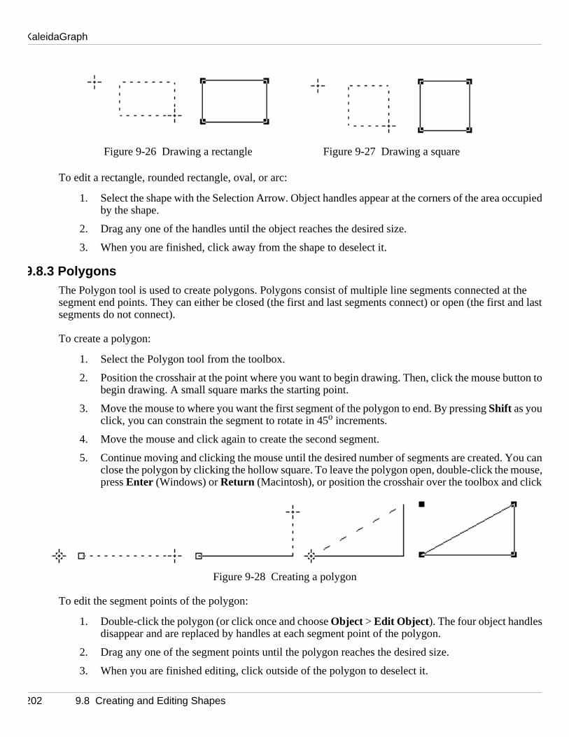
KaleidaGraph
ccupie
t the t and las
tton t
ou caouse
ic
To edit a rectangle, rounded rectangle, oval, or arc:
1. Select the shape with the Selection Arrow. Object handles appear at the corners of the area odby the shape.
2. Drag any one of the handles until the object reaches the desired size.
3. When you are finished, click away from the shape to deselect it.
9.8.3 PolygonsThe Polygon tool is used to create polygons. Polygons consist of multiple line segments connected asegment end points. They can either be closed (the first and last segments connect) or open (the firstsegments do not connect).
To create a polygon:
1. Select the Polygon tool from the toolbox.
2. Position the crosshair at the point where you want to begin drawing. Then, click the mouse buobegin drawing. A small square marks the starting point.
3. Move the mouse to where you want the first segment of the polygon to end. By pressing Shift as youclick, you can constrain the segment to rotate in 45o increments.
4. Move the mouse and click again to create the second segment.
5. Continue moving and clicking the mouse until the desired number of segments are created. Ynclose the polygon by clicking the hollow square. To leave the polygon open, double-click the m,press Enter (Windows) or Return (Macintosh), or position the crosshair over the toolbox and clk
Figure 9-28 Creating a polygon
To edit the segment points of the polygon:
1. Double-click the polygon (or click once and choose Object > Edit Object). The four object handlesdisappear and are replaced by handles at each segment point of the polygon.
2. Drag any one of the segment points until the polygon reaches the desired size.
3. When you are finished editing, click outside of the polygon to deselect it.
Figure 9-26 Drawing a rectangle Figure 9-27 Drawing a square
202 9.8 Creating and Editing Shapes

Working with Plot Tools and Objects
lti-sidennect) o
The ent lines
een th curv
ars and
nt lines.
the x
9.8.4 Bezier CurvesThe Bezier curve tool can be used to draw complex objects. Bezier curves are irregularly shaped, mudobjects that can have curved line segments. They can either be closed (the first and last segments coropen (the first and last segments do not connect).
Each segment in a Bezier curve is defined by four points: two anchor points and two direction points.anchor points determine where the segments begin and end. The direction points, along with the tangthat connect them to the anchor points, determine the size and positioning of the curve segments.
Figure 9-29 Bezier curve definition
Creating a Bezier CurveTo create a Bezier curve:
1. Select the Bezier curve tool from the toolbox.
2. Position the crosshair at the point where you want to begin drawing and click the mouse.
3. Move the mouse until the crosshair is where you want the first segment to end.
4. Click and hold the mouse button down. If you release the button, a straight line appears betwepoints. If you hold down the button and drag, a tangent line appears that allows you to drag theeinto the position you want.
5. Release the mouse button when the segment is the desired shape. The tangent line disappehandles appear at the anchor points.
6. Continue creating more segments and setting the angle and shape of the curve with the tangeThe segments are automatically connected.
7. You can close the curve by clicking the hollow square. To leave the curve open, double-clickmouse, press Enter (Windows) or Return (Macintosh), or position the crosshair over the toolboand click.
Tangent Line
Anchor Point
Direction Point
9.8 Creating and Editing Shapes 203

KaleidaGraph
ht, therehor poin
esire
n point.
aped i
Figure 9-30 Creating a Bezier curve
Editing a Bezier CurveYou can change the position of each anchor point and the shape of each curve. If a segment is straigis no tangent line and you can only change its position. Segments can be deleted by selecting an anctand pressing Backspace (Windows) or Delete (Macintosh).
To edit a Bezier curve:
1. Double-click the curve (or click once and choose Object > Edit Object). The four object handles disappear and are replaced by handles at each anchor point of the curve.
2. Position the arrow over each anchor point you want to move and drag until the point is in the ddposition.
3. Release the mouse button. The tangent line is displayed with round handles at each directioYou can drag these handles to control the size and shape of the curves.
4. Select either of the direction points and drag to edit the shape of the curve. The curve is reshnthe direction you move the handle.
5. Continue moving anchor points and reshaping curves until the curve is the desired shape.
6. When you are finished editing, click outside of the curve to deselect it.
Figure 9-31 Editing a Bezier curve
204 9.8 Creating and Editing Shapes
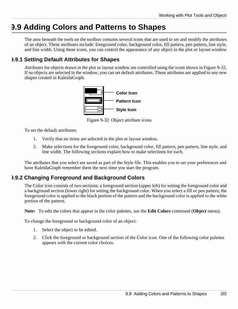
Working with Plot Tools and Objects
attributes style,indow
9-32.any ne
, an
ces and
lor anrn, the whit
ttes
9.9 Adding Colors and Patterns to ShapesThe area beneath the tools on the toolbox contains several icons that are used to set and modify the of an object. These attributes include: foreground color, background color, fill pattern, pen pattern, lineand line width. Using these icons, you can control the appearance of any object in the plot or layout w
9.9.1 Setting Default Attributes for ShapesAttributes for objects drawn in the plot or layout window are controlled using the icons shown in FigureIf no objects are selected in the window, you can set default attributes. These attributes are applied to wshapes created in KaleidaGraph.
Figure 9-32 Object attribute icons
To set the default attributes:
1. Verify that no items are selected in the plot or layout window.
2. Make selections for the foreground color, background color, fill pattern, pen pattern, line styledline width. The following sections explain how to make selections for each.
The attributes that you select are saved as part of the Style file. This enables you to set your preferenhave KaleidaGraph remember them the next time you start the program.
9.9.2 Changing Foreground and Background ColorsThe Color icon consists of two sections: a foreground section (upper left) for setting the foreground coda background section (lower right) for setting the background color. When you select a fill or pen patteeforeground color is applied to the black portion of the pattern and the background color is applied to theportion of the pattern.
Note: To edit the colors that appear in the color palettes, use the Edit Colors command (Object menu).
To change the foreground or background color of an object:
1. Select the object to be edited.
2. Click the foreground or background section of the Color icon. One of the following color paleappears with the current color choices.
Color Icon
Pattern Icon
Style Icon
9.9 Adding Colors and Patterns to Shapes 205

KaleidaGraph
ct lines.rs wheround
ears
3. Select a different color from the palette.
9.9.3 Changing Fill and Pen PatternsThe fill pattern is used to represent the interior of an object. The pen pattern is used to represent objeYou can change the fill or pen pattern by selecting a different pattern from the pop-up menu that appeanyou click the appropriate portion of the Pattern icon. Black portions of the pattern represent the foregcolor and white portions represent the background color.
To change the fill or pen pattern of an object:
1. Select the object to be edited.
2. Click the interior or outer portion of the Pattern icon. One of the following pop-up menus appwith the pattern choices.
Figure 9-35 Fill pattern choices
Figure 9-36 Pen pattern choices
3. Select a different pattern from the pop-up menu.
Figure 9-33 Foreground Color palette Figure 9-34 Background Color palette
206 9.9 Adding Colors and Patterns to Shapes

Working with Plot Tools and Objects
he lin
9.9.4 Changing Line Styles and WidthsThe Style icon controls the line styles and widths used for objects. The left portion of the icon controls testyle; the right portion controls the line width.
To change the line style or line width of an object:
1. Select the object to be edited.
2. Click the line style or line width section of the Style icon. One of the following pop-up menusappears with the available choices.
3. Select a different line style or thickness from the pop-up menu.
Figure 9-37 Line style menu Figure 9-38 Line width menu
9.9 Adding Colors and Patterns to Shapes 207

KaleidaGraph
208 9.9 Adding Colors and Patterns to Shapes

0Working with Curve Fits and Error Bars
Chapter 1 0
rted by
set o using
g, is ith thi
on the, initial
This chapter covers:
• The types of curve fits available in KaleidaGraph.
• Applying a Least Squares curve fit.
• Applying a smoothing curve fit.
• Defining and applying a General (user-defined) curve fit.
• Displaying the results of a curve fit.
• Removing a curve fit from a plot.
• Extrapolating curve fits to the axis limits.
• Adding error bars to a plot.
10.1 Types of Curve FitsThis section provides a brief description and lists the data restrictions for each of the curve fits suppoKaleidaGraph. Refer to Section D.5 for reference information for each of the curve fits.
10.1.1 GeneralThis is the most powerful curve fit in KaleidaGraph. It takes a user-defined equation and uses it to fit afplotted data. Any function of x or m0, where either x or m0 is the independent variable, can be definedup to nine parameters (m1–m9).
Examples:m1 * m0m1 + m2 * m0m1 * exp(–m2 * m0)
When a General curve fit is selected, a curve, defined by the equation in the Curve Fit Definition dialofitted to the data using the Levenberg-Marquardt algorithm. There are no data restrictions associated wscurve fit.
Section 2.5.3 provides a guided tour of defining and applying a General curve fit. For more informationeGeneral curve fit, refer to Sections 10.4–10.5. These sections include details about equation structurguesses, and weighting data.
10.1 Types of Curve Fits 209

KaleidaGraph
ctions
re no
to the he dat
endine no
10.1.2 LinearThis function fits a straight line through your data, of the form y = m0 + m1 * x. There are no data restriassociated with this curve fit.
Note: On a semi-log or log-log plot, this fit appears as a curved line.
10.1.3 PolynomialThis function fits a curve through your data, of the form y = m0 + m1 * x + m2 * x2 + m3 * x3 +...+ m9 * x9.The more complex the curvature of the data, the higher the polynomial order required to fit it. There adata restrictions associated with this curve fit.
10.1.4 ExponentialThis function fits a curve through your data, of the form y = m0 * em1 * x. It is generally used to fit data thatincreases or decreases at a high rate. This curve fit cannot fit negative data or data equal to zero.
Note: On a semi-log plot with a linear X axis, the curve appears as a straight line.
10.1.5 LogarithmicThis function fits a curve through your data, of the form y = m0 + m1 * log(x). A logarithmic curve fit isgenerally used with data that spans decades (100, 101, 102, and so on). This curve fit cannot be used to fit negative data or data equal to zero.
Note: On a semi-log plot with a linear Y axis, the curve appears as a straight line.
10.1.6 PowerThis function fits a curve through your data, of the form y = m0 * xm1. This curve fit cannot be used to fit negative data or data equal to zero.
Note: On a log-log plot, the curve appears as a straight line.
10.1.7 SmoothThis function fits a smoothed curve to the data. KaleidaGraph starts by applying a Stineman functiondata. The output of this function then has a geometric weight applied to the current point and ±10% of tarange, to arrive at the smoothed curve.
The only data restriction associated with this curve fit is that the independent (X) variable must be in ascgorder in the data window. There is no single expression that represents this curve; therefore, there arparameters to view or copy.
210 10.1 Types of Curve Fits
Working with Curve Fits and Error Bars
t of thiitting tliers. a ver
endine no
s a line
endine no
. The n happe
endine no
izes thhnique f bein
int is , the simple
re:
mple. ed tou
10.1.8 WeightedThis function fits a curve to the data, using the locally weighted Least Squared error method. The resulscurve fit is to plot a best fit smooth curve through the center of the data. This is an extremely robust ftechnique. Unlike the standard Least Squared error method, this technique is nearly insensitive to ouHowever, this does not come for free. The Weighted curve fit is computationally complex and can takeylong time for a large data set.
The only data restriction associated with this curve fit is that the independent (X) variable must be in ascgorder in the data window. There is no single expression that represents this curve; therefore, there arparameters to view or copy.
10.1.9 Cubic SplineMoving left to right along the curve in increasing X, every group of four consecutive data points definecubic polynomial equation. A series of these cubic polynomials connected together define a cubic spcurve. Using this curve fit is similar to using a French curve to connect all of the data points.
The only data restriction associated with this curve fit is that the independent (X) variable must be in ascgorder in the data window. There is no single expression that represents this curve; therefore, there arparameters to view or copy.
10.1.10 InterpolateThis function fits a curve that passes through the data points and matches the slopes at those pointsadvantage of this curve fit is that it does not produce wild results near an abrupt change of slope, as canwith the Cubic Spline curve fit.
The only data restriction associated with this curve fit is that the independent (X) variable must be in ascgorder in the data window. There is no single expression that represents this curve; therefore, there arparameters to view or copy.
10.2 Applying a Least Squares FitLeast Squares is a method of curve fitting that has been popular for a long time. Least Squares minimesquare of the error between the original data and the values predicted by the equation. While this tecmay not be the most statistically robust method of fitting a function to a data set, it has the advantage ogrelatively simple (in terms of required computing power) and of being well understood.
The major weakness of the Least Squared method is its sensitivity to outliers in the data. If a data powidely different from the majority of the data, it can skew the results of the regression. For this reasondata should always be examined for reasonableness before fitting. The Data Selection tool provides amethod of removing outliers from a plot. The use of this tool is covered in Section 9.4.
The Curve Fit menu contains several curve fits that use the Least Squares method. These curve fits aLinear, Polynomial, Exponential, Logarithmic, and Power. For descriptions and any data restrictions associated with these curve fits, see Sections 10.1.2–10.1.6.
The following steps explain how to apply a Least Squares fit, using the Polynomial curve fit as an exaThe procedure is basically the same for applying the other Least Square fits. Section 2.2.4 in the guidrincludes an example of applying a Linear curve fit.
10.2 Applying a Least Squares Fit 211

KaleidaGraph
.
All
is
To apply a Polynomial curve fit:
1. Open the plot window which will have the curve fit applied. Figure 10-1 shows a sample plot
Figure 10-1 Sample plot
2. Choose Curve Fit > Polynomial. A Curve Fit Selections dialog similar to Figure 10-2 appears. dependent variables are listed under Column Names.
Figure 10-2 Curve Fit Selections dialog
3. Click the check box for each variable to be fit. A keyboard shortcut (Ctrl +A under Windows or +A on a Macintosh) is available to select all of the variables at once. Each time a variable
selected, a second dialog appears (Figure 10-3). Use this dialog to specify the order of the polynomial to be fit. The maximum value that can be selected is nine.
Note: This extra dialog is only displayed when using the Polynomial fit.
Figure 10-3 Polynomial Order dialog
-0.4-0.2
00.20.40.60.8
1
-2 -1.5 -1 -0.5 0 0.5 1 1.5 2
Sinc(5x)
Sin
c(5x
)
-π/2 to π/2
212 10.2 Applying a Least Squares Fit

Working with Curve Fits and Error Bars
ts. le plot
fits are:ed with
e. Th
.
4. Click OK to exit each dialog and apply the curve fit.
After the curve fit is applied, you can display its equation or extrapolate the fit to the axis limiThese are a few of the features covered in Sections 10.6–10.8. Figure 10-4 shows the sampafter applying a Polynomial curve fit and displaying the equation.
Figure 10-4 Sample plot with Polynomial curve fit applied
10.3 Applying a Smoothing FitThe Curve Fit menu contains four commands designed to fit a smooth curve to the data. These curve Smooth, Weighted, Cubic Spline, and Interpolate. For descriptions and any data restrictions associatthese curve fits, see Sections 10.1.7–10.1.10.
The following steps explain how to apply a smoothing fit, using the Cubic Spline curve fit as an exampleprocedure is basically the same for applying the other smoothing fits.
To apply a Cubic Spline curve fit:
1. Open the plot window which will have the curve fit applied. Figure 10-5 shows a sample plot
Figure 10-5 Sample plot
-0.4-0.2
00.20.40.60.8
1
-2 -1.5 -1 -0.5 0 0.5 1 1.5 2
Sinc(5x)
Sin
c(5x
)
-π/2 to π/2
Y = M0 + M1*x + ... M8*x8 + M9*x9
0.74498M0
-2.2335e-06M1
-1.5263M2
5.3462e-06M3
0.57926M4
-2.3478e-06M5
0.89451R
0
1
2
3
4
5
6
7
0 2 4 6 8 10 12 14
example #1
Test #1Test #2
Ran
ge
Time
10.3 Applying a Smoothing Fit 213

KaleidaGraph
Al
d. Us
l dat
2. Choose Curve Fit > Cubic Spline. A Curve Fit Selections dialog similar to Figure 10-6 appears. ldependent variables are listed under Column Names.
Figure 10-6 Curve Fit Selections dialog
3. Click the check box for each variable to be fit. A keyboard shortcut (Ctrl +A under Windows or +A on a Macintosh) is available to select all of the variables at once.
Note: When applying a Weighted fit, a second dialog appears each time a variable is selecteethis dialog to specify the smoothing factor.
4. Click OK to apply the curve fit.
After the curve fit is applied, you can increase the number of curve fit points or hide the originaato only display the curve fit. These are a few of the features covered in Sections 10.6–10.8. Figure 10-7 shows the sample plot after applying a Cubic Spline curve fit.
Figure 10-7 Sample plot with Cubic Spline curve fit applied
0
1
2
34
5
6
7
0 2 4 6 8 10 12 14
example #1
Test #1Test #2
Ran
ge
Time
214 10.3 Applying a Smoothing Fit

Working with Curve Fits and Error Bars
enerarquarduatio
s, the
sam
enterelue.
same)
finition1, m2, in th
d als
.
10.4 General Curve Fit BasicsNonlinear curve fitting is accommodated in KaleidaGraph through the General curve fit function. The Glcurve fit can be used to define your own equation and apply a fit to the data, using the Levenberg-Matalgorithm. This is the most powerful curve fit in KaleidaGraph because you can specify virtually any eqnto be fitted to the data.
This section explains the structure of the curve fit equation, setting initial conditions for the parameterCurve Fit Definition dialog, and the use of the commands in the General submenu.
10.4.1 Curve Fit DefinitionThe curve fit definition is the equation that is fitted to the data. Curve fit definitions are composed of theeitems as formulas in Formula Entry: operators, parameters, functions, and constants, in addition to anindependent variable. When entering the curve fit definition, follow these guidelines:
• The independent variable in an equation is represented by m0.
• The parameters being calculated by the fit are represented by m1–m9. Parameters should bedwherever you have an unknown quantity and you want KaleidaGraph to calculate the best va
• Use an asterisk (*) for multiplication and a caret (^) for raising quantities to a power.
• KaleidaGraph does not distinguish between upper and lower case letters (m0 and M0 are the
• Constants and other shorthand references can be defined in the library for use in a curve fit de.Some definitions in the default library are used to substitute x for m0, and a, b, c, and d for mm3, and m4, respectively. Section 10.5.7 provides an example of defining a curve fit equationelibrary.
• To include a column number as part of the curve fit definition, the table function must be used. Section 10.5.5 shows how to use the table function in a General curve fit definition. This methooenables you to fit equations containing multiple independent variables.
The following table lists some equations and how they appear as curve fit definitions in KaleidaGraph
Original Equations Curve Fit Definitions
a * x + b m1 * m0 + m2
a + b * x^c m1 + m2 * m0^m3
a + b * exp(–c * x) m1 + m2 * exp(–m3 * m0)
a * exp(–b * x) * cos(c * x + d) m1 * exp(–m2 * m0) * cos(m3 * m0 + m4)
10.4 General Curve Fit Basics 215

KaleidaGraph
e for t it in the
lues
are nognitude
e enelow
used i
an
10.4.2 Initial ConditionsEven though KaleidaGraph calculates values for unknown parameters, you must supply an initial valueach parameter. The algorithm used to calculate the final results requires a reasonable guess to poinright direction. KaleidaGraph improves upon these values during each iteration of the fit.
Note: Since the fit starts with initial guesses and improves upon them with each iteration, the final vamay be different for a separate set of initial guesses.
Do not get carried away trying to find good guesses; the initial conditions are just that, guesses. If youtsure what the guesses should be, keep the initial conditions non-zero, and at the correct order of mathat you might expect (be it 0.001, 1, or 1000).
The initial conditions are entered immediately following the curve fit definition. Place a semicolon at thdof the definition and begin entering the initial guesses, separating each with a semicolon. The table bshows the definitions from the previous section with some sample initial guesses.
10.4.3 Curve Fit Definition DialogThe Curve Fit Definition dialog is used to enter the equation, initial guesses, and allowable error to be nthe curve fit. You can also choose to specify partial derivatives or to weight the data.
This dialog can be displayed using either of the following methods:
• Choose a curve fit from the General submenu (Curve Fit menu). In the dialog that is displayed, clickDefine.
• Choose Curve Fit > Edit General. In the dialog that is displayed, select the name of a curve fit dclick Edit .
The various features of the Curve Fit Definition dialog are discussed below.
Curve Fit Definitions with Initial Guesses
m1 * m0 + m2; m1 = 0.5; m2 = 23
m1 + m2 * m0^m3; m1 = –2; m2 = 3; m3 = 2
m1 + m2 * exp(–m3 * m0); m1 = 5; m2 = 1; m3 = 0.5
m1 * exp(–m2 * m0) * cos(m3 * m0 + m4); m1 = 4; m2 = 0.7; m3 = 2.2; m4 = 15
216 10.4 General Curve Fit Basics

Working with Curve Fits and Error Bars
p if
. Thess: ected,
es
log
Figure 10-8 Curve Fit Definition dialog
1. Text FieldCurve fit definitions and initial guesses are entered in this area of the dialog.
2. Allowable Error:The value entered in this field helps KaleidaGraph determine when to stop iterating. Iterations stoeither of the following occurs:
• Chi Square does not change for a certain number of iterations.
• The percent change in the normalized Chi Square is less than the Allowable Error.
3. Weight DataWhen selected, you can specify a data column that contains weights for the variable you are fittingeweights should represent the individual errors of the data values. Each weight is used internally a1/(weight^2). The smaller the error value, the larger the internal weight. If this check box is not sela weight value of 1.0 is used for all data points.
4. Specify PartialsThe algorithm that KaleidaGraph uses in calculating each iteration of the General curve fit requirevaluating the partial derivative of the function with respect to each parameter. If Specify Partials is notselected, KaleidaGraph numerically approximates the derivative. If this option is selected, the diaexpands, as shown in Figure 10-9.
1
2
3
5
7
6
4
10.4 General Curve Fit Basics 217

KaleidaGraph
field urve fit e besactual
et tive i
.
inition.
Figure 10-9 Expanded Curve Fit Definition dialog
The nine buttons at the bottom of the dialog allow each partial derivative to be entered in the textabove the buttons. The biggest advantage of specifying the partial derivatives is accuracy. The calgorithm uses these partial derivatives to direct itself where to move after each iteration to find thtsolution. In general, sharp deviations in the surface may not be accurately approximated, so the partial derivatives are preferred.
You can choose to specify only some of the partial derivatives, but not all of them. It is better to lKaleidaGraph approximate the partial instead of specifying the wrong derivative. If a partial derivasmissing, KaleidaGraph numerically approximates that partial derivative.
5. Degrees/Radians ButtonsThese buttons determine whether the results of trigonometric functions are in degrees or radians
6. Help...Click this button to display the Help dialog.
7. File...Clicking this button displays a text editor that can be used to create, open, or save a curve fit defThe definition appears on the first line and any partial derivatives appear on the lines below it.
218 10.4 General Curve Fit Basics

Working with Curve Fits and Error Bars
16lain ho
nge
t ar
hed.
10.4.4 Managing the Curve Fit ListKaleidaGraph maintains a master list of curve fits in the General submenu. This submenu can store up to user-defined equations that can be applied whenever a new plot is created. The following sections expwto edit and save changes to the curve fits listed in the General submenu.
Note: The only way to edit the master list is to create a new plot and use the Edit General command. The master list is not affected if you do either of the following:
• Use a saved plot (or any plot that had its data archived).
• Choose a curve fit from the General submenu and click Define to edit the definition.
Adding a Curve Fit to the Master ListTo add a curve fit to the master curve fit list:
1. Create a new plot.
2. Choose Curve Fit > General > Edit General.
3. Select a fit in the current list.
4. Click Add and a New Fit appears below the selected fit in the list. The name of the fit can be chadby selecting it and editing the name in the text field.
5. Click Edit to enter the definition in the Curve Fit Definition dialog.
6. Click OK when you are finished. Now you can use this fit in the active plot or any new plots thaecreated. Remember to save changes to the Macros file to make the changes permanent.
Rearranging the Master Curve Fit ListTo rearrange the curve fit list:
1. Create a new plot.
2. Choose Curve Fit > General > Edit General.
3. Select the curve fit to be repositioned.
4. Click Copy to copy the fit to the trash bin.
5. Click Remove to delete the name from the listing.
6. Select a curve fit in the current list.
7. Select the name of the curve fit that was copied to the trash bin.
8. Click Add and the curve fit appears below the selected fit in the list.
Note: When rearranging curve fits, do not leave the Edit General dialog until you are completely finisAs soon as you click OK or Cancel in this dialog, anything in the trash bin is deleted. The only permanent trash bin item is New Fit.
10.4 General Curve Fit Basics 219
KaleidaGraph
plot r curv
w
ros
s
Removing a Curve Fit from the Master ListTo remove a curve fit from the master list:
1. Create a new plot.
2. Choose Curve Fit > General > Edit General.
3. Select the curve fit to be deleted.
4. Click Remove to delete the curve fit from the listing.
5. Click OK .
Adding Curve Fits from the Master List to Saved PlotsWhen a saved plot is opened, the General submenu displays the curve fits that were available when the was originally created, regardless of what is currently in the master list. To add curve fits from the masteefit list to a saved plot:
1. Open a saved plot.
2. Choose Curve Fit > General > Edit General. The curve fits stored in the master list appear belothe dotted line in the trash bin.
3. Select the name of the curve fit to be added from the trash bin listing.
4. Select a fit in the current list.
5. Click Add and the curve fit appears below the selected fit in the list.
6. Click OK when you are finished. Now you can use this fit in the saved plot.
Saving Changes to the Curve Fit MenuThe curve fits in the General submenu are saved, by default, in a file called KGMacros (Windows) or KG Macros (Macintosh). This file is loaded each time you start KaleidaGraph.
To save any changes made to the Curve Fit menu, it is necessary to save the changes to the default Macfile using one of the following methods:
• Choose File > Preferences and select Prompt from the Macros pop-up menu. When exiting KaleidaGraph, a dialog asks whether or not to overwrite the Macros file that was opened at launch.
• Choose File > Preferences and select Always from the Macros pop-up menu. When exiting KaleidaGraph, the Macros file that was opened at launch is automatically overwritten.
• Choose File > Export > Macros and overwrite the default Macros file.
Note: Only changes made to a new plot using the Edit General command are saved as part of the macrofile. Any changes made to a saved plot or by choosing a curve fit from the General submenu and clicking Define apply solely to that particular plot.
220 10.4 General Curve Fit Basics
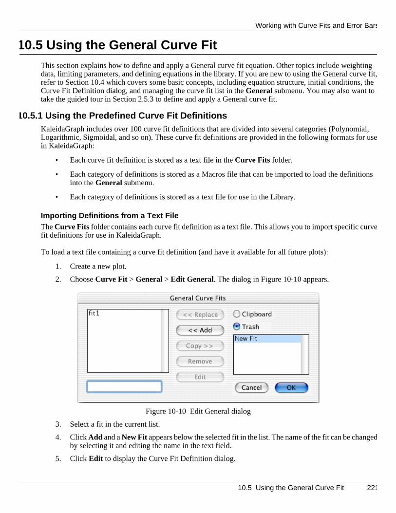
Working with Curve Fits and Error Bars
hting rve fit,s, the
ial, r use
tions
urv
nge
10.5 Using the General Curve FitThis section explains how to define and apply a General curve fit equation. Other topics include weigdata, limiting parameters, and defining equations in the library. If you are new to using the General curefer to Section 10.4 which covers some basic concepts, including equation structure, initial conditionCurve Fit Definition dialog, and managing the curve fit list in the General submenu. You may also want totake the guided tour in Section 2.5.3 to define and apply a General curve fit.
10.5.1 Using the Predefined Curve Fit DefinitionsKaleidaGraph includes over 100 curve fit definitions that are divided into several categories (PolynomLogarithmic, Sigmoidal, and so on). These curve fit definitions are provided in the following formats foin KaleidaGraph:
• Each curve fit definition is stored as a text file in the Curve Fits folder.
• Each category of definitions is stored as a Macros file that can be imported to load the definiinto the General submenu.
• Each category of definitions is stored as a text file for use in the Library.
Importing Definitions from a Text FileThe Curve Fits folder contains each curve fit definition as a text file. This allows you to import specific cefit definitions for use in KaleidaGraph.
To load a text file containing a curve fit definition (and have it available for all future plots):
1. Create a new plot.
2. Choose Curve Fit > General > Edit General. The dialog in Figure 10-10 appears.
Figure 10-10 Edit General dialog
3. Select a fit in the current list.
4. Click Add and a New Fit appears below the selected fit in the list. The name of the fit can be chadby selecting it and editing the name in the text field.
5. Click Edit to display the Curve Fit Definition dialog.
10.5 Using the General Curve Fit 221

KaleidaGraph
ureult.
newrmanen
ese
ated
ecaus
ade
ns for
the l
6. Click File in the Curve Fit Definition dialog. A text editor appears.
7. Choose File > Open.
8. Locate and open a curve fit definition from the Curve Fits folder. The definition and initial guessesfor the parameters will be displayed in the editor.
9. Choose File > Close to display the curve fit equation in the Curve Fit Definition dialog. Make syou change the initial guesses, because all of the initial guesses are set equal to 1.0 by defa
10. Click OK until you return to the plot window. Now you can use this fit in the active plot or any plots that are created. Remember to save changes to the Macros file to make the changes pet
Importing Definitions from a Macros FileThe Macros folder contains a Macros file for each category of curve fit definitions. Importing one of thMacros files loads the curve fit definitions into the General submenu.
Note: If a plot is already open, you will not see the imported curve fit definitions until a new plot is cre
To load the definitions from a Macros file:
1. Choose File > Open.
2. Locate and open the Macros file of interest from the Macros folder.
3. Create a new plot. The curve fit definitions stored in the Macros file will be listed under the Generalsubmenu.
4. You can now apply one of these fits to your data. Make sure you change the initial guesses, beall of the initial guesses are set equal to 1.0 by default.
Importing Definitions into the LibraryThe Library folder contains text files for each category of curve fit definitions. These text files can be lodinto the library for use in the General curve fit.
To load a text file into the library:
1. Choose Macros > Library or Curve Fit > General > Library .
2. Choose File > Open.
3. Locate and open the curve fit category of interest from the Library folder.
4. Browse through the library and make note of the shorthand reference and number of unknowthe curve fits that you will be using.
5. Choose File > Close.
You can now use these library definitions to apply a General curve fit. When entering the definition inCurve Fit Definition dialog, you can enter the shorthand reference defined in the library with the initiaguesses, for example gaussfit(1,5,1,10). KaleidaGraph will perform the necessary substitutions before applying the fit.
222 10.5 Using the General Curve Fit

Working with Curve Fits and Error Bars
ly ente
nge
l tion an
newrmanen
10.5.2 Entering a Custom Curve Fit DefinitionIf you need to use a curve fit equation that is not included with the predefined equations, you can easira custom equation and use it in KaleidaGraph.
Note: Custom curve fit equations can also be defined in the library. Refer to Section 10.5.7 for moreinformation on this topic.
To create a custom curve fit definition (and have it available for all future plots):
1. Create a new plot.
2. Choose Curve Fit > General > Edit General.
3. Select a fit in the current list.
4. Click Add and a New Fit appears below the selected fit in the list. The name of the fit can be chadby selecting it and editing the name in the text field.
5. Click Edit to display the Curve Fit Definition dialog.
6. Enter the curve fit equation in the Curve Fit Definition dialog. Make sure you include the initiaguesses for each of the unknown parameters. Figure 10-11 shows an example curve fit equadits initial guesses.
Figure 10-11 Example curve fit equation
7. Click OK until you return to the plot window. Now you can use this fit in the active plot or any plots that are created. Remember to save changes to the Macros file to make the changes pet
10.5 Using the General Curve Fit 223

KaleidaGraph
t.
be
.
10.5.3 Applying a General Curve FitTo apply a General curve fit:
1. Open the plot window which will have the curve fit applied. Figure 10-12 shows a sample plo
Figure 10-12 Sample plot
2. Choose a curve fit from the General submenu (Curve Fit menu). A Curve Fit Selections dialog similar to Figure 10-13 appears. All dependent variables are listed under Column Names.
Figure 10-13 Curve Fit Selections dialog
3. If the equation has not been entered, click Define to enter the equation or shorthand reference toapplied to the data. Figure 10-14 shows the Curve Fit Definition dialog containing a curve fit definition. When you are finished, click OK .
Note: For information on including this fit in your master curve fit list, refer to Section 10.4.4
4
6
8
10
12
14
16
-80 -60 -40 -20 0 20 40 60 80
Data 1B
224 10.5 Using the General Curve Fit
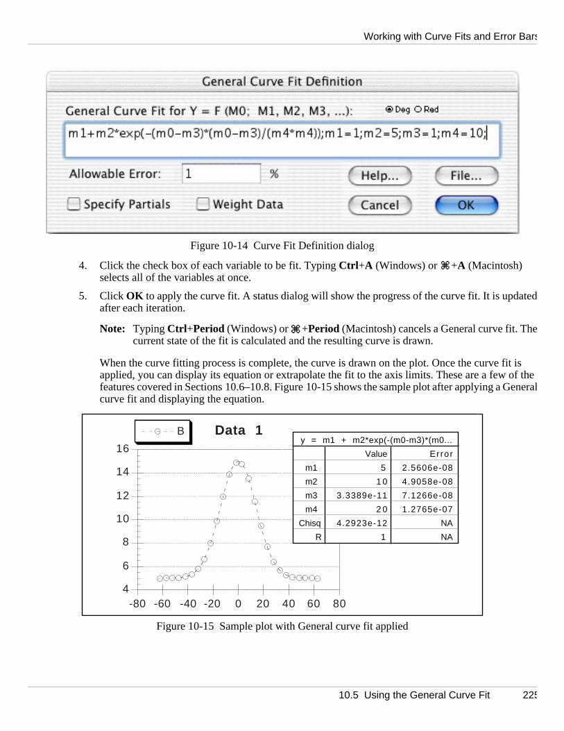
Working with Curve Fits and Error Bars
ate
t is of the
enera
Figure 10-14 Curve Fit Definition dialog
4. Click the check box of each variable to be fit. Typing Ctrl +A (Windows) or +A (Macintosh) selects all of the variables at once.
5. Click OK to apply the curve fit. A status dialog will show the progress of the curve fit. It is upddafter each iteration.
Note: Typing Ctrl +Period (Windows) or +Period (Macintosh) cancels a General curve fit. Thecurrent state of the fit is calculated and the resulting curve is drawn.
When the curve fitting process is complete, the curve is drawn on the plot. Once the curve fiapplied, you can display its equation or extrapolate the fit to the axis limits. These are a few features covered in Sections 10.6–10.8. Figure 10-15 shows the sample plot after applying a Glcurve fit and displaying the equation.
Figure 10-15 Sample plot with General curve fit applied
4
6
8
10
12
14
16
-80 -60 -40 -20 0 20 40 60 80
Data 1By = m1 + m2*exp(-(m0-m3)*(m0...
Er rorValue
2.5606e-085m1
4.9058e-081 0m2
7.1266e-083.3389e-11m3
1.2765e-072 0m4
NA4.2923e-12Chisq
NA1R
10.5 Using the General Curve Fit 225

KaleidaGraph
olumn
ses theduce
ppears.
nctiove fit.
ting o
of the
f false,
ndar
t a
10.5.4 Weighting DataThe General curve fit provides an option to weight the data. When Weight Data is selected in the Curve FitDefinition dialog, the data is weighted during the curve fit. These weights are taken from a specified cin the data window. The weights should represent the individual error values of the fitted data.
Each weight is used internally as: 1/(weight^2). Specifying a weight less than 1.0 for a data point increaeinternal weight of that point and can make the total error much larger. Weight values larger than 1.0 rthe internal weights. When Weight Data is not selected, a weight value of 1.0 is used for all data points.
When the Weight Data option is selected and you choose a variable to fit, the dialog in Figure 10-16 aUse this dialog to select the column containing the weights for your data.
Figure 10-16 Selecting column of weights
10.5.5 Fitting Equations with Multiple Independent VariablesThrough the use of the table function, KaleidaGraph can fit equations containing multiple independent variables. For example, to fit an equation like y = a*x + b*x2 +c, you would enter the following curve fit definition: a*x + b*table(m0, x col, x2 col) + c. You need to replace x col and x2 col with the appropriate column numbers from the data window (for example, table(m0, c0, c2)). The result of using the table funis that for each value of x, the corresponding value from the x2 column is evaluated as part of the cur
10.5.6 Setting Limits for Curve Fit Parameters Limits on curve fit parameters can be set in one of two ways. The first method is to use conditional tesnthe parameter. The second method is to use the limit function from the default library.
Suppose that a General curve fit is being defined to fit a straight line to a set of data. The equation isform: a+b*x. In this example, you want to limit the value of b so that it is not a negative number.
In the Curve Fit Definition dialog, enter either of the following definitions:
a + (b=(b<0) ? 0 : b) *x; a=1; b=1 or a + (b=limit(0, 1000, b))*x; a=1; b=1
In the first definition, a conditional test is performed to see if b is less than zero. If true, b is set to zero; ib is set equal to itself.
In the second definition, the limit function is used. The limit function requires that a lower and upper bouybe set for the parameter. In this case, zero and 1000 are used to bound the extremes of b.
Whenever a parameter is bound in a General curve fit definition, you must specify partial derivatives.Otherwise, a Singular Coefficient Matrix error may occur if the parameter being limited gets pegged abounding point for multiple iterations.
226 10.5 Using the General Curve Fit
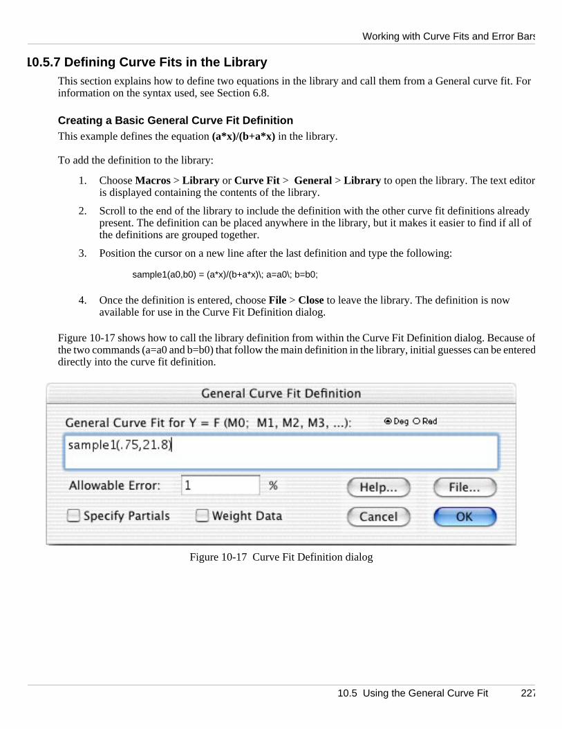
Working with Curve Fits and Error Bars
t. For
dy all of
e ontere
10.5.7 Defining Curve Fits in the LibraryThis section explains how to define two equations in the library and call them from a General curve fiinformation on the syntax used, see Section 6.8.
Creating a Basic General Curve Fit DefinitionThis example defines the equation (a*x)/(b+a*x) in the library.
To add the definition to the library:
1. Choose Macros > Library or Curve Fit > General > Library to open the library. The text editoris displayed containing the contents of the library.
2. Scroll to the end of the library to include the definition with the other curve fit definitions alreapresent. The definition can be placed anywhere in the library, but it makes it easier to find if the definitions are grouped together.
3. Position the cursor on a new line after the last definition and type the following:
sample1(a0,b0) = (a*x)/(b+a*x)\; a=a0\; b=b0;
4. Once the definition is entered, choose File > Close to leave the library. The definition is now available for use in the Curve Fit Definition dialog.
Figure 10-17 shows how to call the library definition from within the Curve Fit Definition dialog. Becausfthe two commands (a=a0 and b=b0) that follow the main definition in the library, initial guesses can be eddirectly into the curve fit definition.
Figure 10-17 Curve Fit Definition dialog
10.5 Using the General Curve Fit 227

KaleidaGraph
This
addeses al
into on in the
ame
Creating a Complex General Curve Fit Definition Now that a basic curve fit definition has been defined, let’s create a more complex curve fit definition.example creates a definition for the following equation:
a*exp(–(x–b)^2/(c*c)) + d*exp(–(x–f)^2/(g*g)) + h*exp(–(x–i)^2/(j*j))
To add this definition to the library:
1. Open the library again so that the definition can be added. The following commands should bedto the existing Variable Definitions. These commands are necessary to define a formula that ulof the parameters available (m1–m9).
f=m5;g=m6;h=m7;i=m8;j=m9;
2. Add the following commands to the existing Curve Fit Definitions.form1() = a*exp(–(x–b)^2/(c*c));;form2() = d*exp(–(x–f)^2/(g*g));;form3() = h*exp(–(x–i)^2/(j*j));;sample2(a0, b0, c0, d0, f0, g0, h0, i0, j0) = form1() + form2() + form3()\;a=a0\; b=b0\; c=c0\; d=d0\; f=f0\; g=g0\; h=h0\; i=i0\; j=j0;
Notice the original equation has been split into three smaller parts and all three parts are tied togethereformula. This makes it possible to use curve fit definitions that are longer than the 256 character limitCurve Fit Definition dialog.
Figure 10-18 shows how to call the library definition from within the Curve Fit Definition dialog. The nof the definition is entered, followed by all of the initial guesses.
Figure 10-18 Curve Fit Definition dialog
228 10.5 Using the General Curve Fit
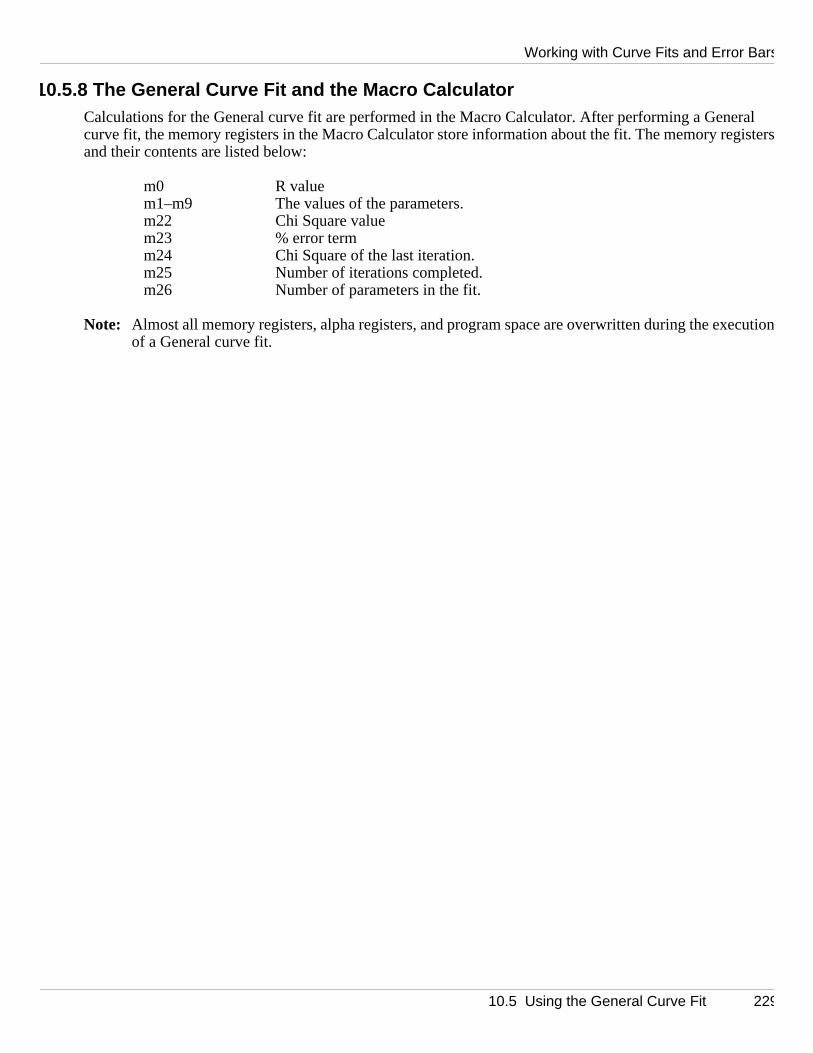
Working with Curve Fits and Error Bars
ral gisters
ecutio
10.5.8 The General Curve Fit and the Macro CalculatorCalculations for the General curve fit are performed in the Macro Calculator. After performing a Genecurve fit, the memory registers in the Macro Calculator store information about the fit. The memory reand their contents are listed below:
m0 R valuem1–m9 The values of the parameters.m22 Chi Square valuem23 % error termm24 Chi Square of the last iteration.m25 Number of iterations completed.m26 Number of parameters in the fit.
Note: Almost all memory registers, alpha registers, and program space are overwritten during the exnof a General curve fit.
10.5 Using the General Curve Fit 229

KaleidaGraph
tion o
lot ation
l and ger thaw.
zeros
10.6 Working with Curve Fit ResultsThis section explains how to view the results of a curve fit, interpret the values that are reported by KaleidaGraph, and export the curve fit results for further analysis.
10.6.1 Viewing Curve Fit ResultsKaleidaGraph provides two methods to view the results of a curve fit. You can either display the equanthe plot or view the coefficients in a dialog.
Displaying the Curve Fit EquationThe curve fit equation can be displayed by turning on Display Equation in the Plot menu. The results from any General, Linear, Polynomial, Exponential, Logarithmic, or Power curve fits are displayed in the pwindow. Not only is the resulting equation displayed, but if any updates occur to the curve fit, the equupdates automatically.
Depending on the type of curve fit, the equation is displayed in a table or as a text label. The GeneraPolynomial curve fits display equations in a table because the equations for these fits can be much lonnthe others. The appearance of the equation can be edited by double-clicking it with the Selection Arro
The numeric format of the equation can be controlled using the Equation Label Format command (Formatmenu). Some of the options available include number format, number of significant digits, and trailing
Viewing CoefficientsThe other method of displaying curve fit results is to view the curve fit’s coefficients in a dialog.
To view the coefficients from the curve fit:
1. Reselect the curve fit from the Curve Fit menu. A Curve Fit Selections dialog similar to Figure 10-19 appears with a drop-down arrow under View for each variable that has a curve fit applied.
Figure 10-19 Curve Fit Selections dialog
2. Click one of the drop-down arrows and choose View Results from the pop-up menu that appears. Adialog similar to Figure 10-20 will be displayed containing the coefficients from the curve fit.
230 10.6 Working with Curve Fit Results

Working with Curve Fits and Error Bars
t
ial, se fits
io
te the
sent th
quared e, the
Figure 10-20 Viewing coefficients
3. To copy the coefficients to the Clipboard, click Clipboard . This enables you to paste the results inoanother window or program.
4. To copy the coefficients to the Calculator, click Calculator. This enables you to use the results inaFormula Entry function.
5. Click OK until you return to the plot window.
10.6.2 Interpreting Curve Fit ResultsThis section explains some of the values that are calculated when using the General, Linear, PolynomExponential, Logarithmic, and Power curve fits. The correlation coefficient is calculated for each of the,but only the General curve fit displays the parameter errors and Chi Square value.
Correlation CoefficientsA correlation coefficient (R or R2) is displayed with the curve fit’s equation and coefficients. The correlatncoefficient indicates how well the calculated curve fits the original data.
This value ranges from zero to one. The closer to one, the better the fit. The equation used to calculacorrelation coefficient is listed in Section D.6.
You can choose to display the Linear Correlation Coefficient (R) or the Coefficient of Determination (R2) aspart of the results. The Display R^2 instead of R check box in the Curve Fit Options dialog (Format menu)controls which is displayed.
Parameter ErrorsThe General curve fit displays a column of errors to the right of the parameter values. The errors repreestandard error values of the parameters. These values should be read as: parameter value ± error.
Chi Square ValueThe General curve fit reports a Chi Square value as part of the results. This value is the sum of the serror between the original data and the calculated curve fit. In general, the lower the Chi Square valubetter the fit. The equation used to calculate Chi Square is listed in Section D.6.
10.6 Working with Curve Fit Results 231

KaleidaGraph
optionrve fit
sults
if th
sults
10.6.3 Exporting Curve Fit ResultsOnce a curve fit has been applied, the results of the fit can be exported for further analysis. The exportsinclude copying the parameter values to the Clipboard or the Calculator, copying the values of the culine into the data window, and copying the residual values into the data window.
Copying the Parameters to the Clipboard or CalculatorTo copy the parameter values to the Clipboard or Calculator:
1. Reselect the curve fit from the Curve Fit menu. A Curve Fit Selections dialog similar to Figure 10-21 appears with a drop-down arrow under View for each variable that has a curve fit applied.
Figure 10-21 Curve Fit Selections dialog
2. To copy the coefficients to the Clipboard, click one of the drop-down arrows and choose Copy Parameters to Clipboard from the pop-up menu that appears. This enables you to paste the reinto another window or program.
Note: If you paste the results into the plot window, the coefficients in the table do not changeecurve fit is updated. For this reason, we recommend that you use the Display Equation command instead.
3. To copy the coefficients to the Calculator, click one of the drop-down arrows and choose Copy Parameters to Calculator from the pop-up menu that appears. This enables you to use the rein a Formula Entry function.
4. Click OK to return to the plot window.
Note: It is also possible to copy the parameters by choosing View Results from the pop-up menu and clickingthe Clipboard or Calculator button.
Copying the Curve Fit Values to the Data WindowTo copy the values of the curve fit line to the data window:
1. Reselect the curve fit from the Curve Fit menu. A Curve Fit Selections dialog similar to Figure 10-21 appears with a drop-down arrow under View for each variable that has a curve fit applied.
2. Click one of the drop-down arrows and choose Copy Curve Fit to Data Window from the pop-upmenu that appears.
3. Click OK to return to the plot window.
232 10.6 Working with Curve Fit Results

Working with Curve Fits and Error Bars
ll be value
Entryns in
s
chec
le is
KaleidaGraph will append the results after any existing data in your data window. The first column wiaseries of X values. Except for the Weighted curve fit which uses the original X values, the number of X swill be equal to the number of curve fit points specified in the Curve Fit Options dialog (Format menu). Thesecond column will contain the values from the curve fit at each of these locations.
Note: If you want to use the original X values or supply your own X values, you need to use Formulato calculate the curve fit values. Section 6.6 provides instructions for using the curve fit functioFormula Entry to obtain values from the curve fit.
Copying the Residuals to the Data WindowTo copy the residual values to the data window:
1. Reselect the curve fit from the Curve Fit menu. A Curve Fit Selections dialog similar to Figure 10-21 appears with a drop-down arrow under View for each variable that has a curve fit applied.
2. Click one of the drop-down arrows and choose Copy Residuals to Data Window from the pop-upmenu that appears.
3. Click OK to return to the plot window.
KaleidaGraph will append the residual values after any existing data in the data window. These valuerepresent the difference between the original Y values and the values calculated by the curve fit.
10.7 Removing a Curve FitCurve fits can be removed from a plot in the same way that they are added. After applying a curve fit, akmark appears next to that type of fit in the Curve Fit menu to indicate that a curve fit is applied.
To remove a curve fit from the plot:
1. From the Curve Fit menu, choose the type of curve fit to be removed. A dialog similar to Figure 10-22 is displayed containing the list of variables. The check box of each fitted variabselected.
Figure 10-22 Curve Fit Selections dialog
2. Clear any check boxes for the fits to be removed. Clicking Deselect clears all of the check boxes atonce.
3. Click OK to return to the plot and remove the curve fits and any associated equations.
10.7 Removing a Curve Fit 233

KaleidaGraph
ptions
enden of the
olate)
the
10.8 Other Curve Fit FeaturesThe following sections show how to use some of the options available for curve fits. Some of these oinclude extrapolating to the axis limits and increasing the number of curve fit points.
The line style, width, and color of the curve fit are controlled using the Plot Style command (Plot menu). Themethod for changing these settings is described in Section 8.9.4.
10.8.1 Extrapolating to the Axis LimitsCurve fits are normally displayed between the minimum and maximum data values plotted on the indeptaxis. However, you can choose to extrapolate the curve fits to the axis limits. The extrapolated portionfit is based on the calculated equation.
Note: It is not possible to extrapolate the Smoothing fits (Smooth, Weighted, Cubic Spline, and Interpbecause they cannot be represented by a single equation.
To extrapolate a curve fit:
1. Choose Format > Curve Fit Options. The dialog in Figure 10-23 appears.
Figure 10-23 Curve Fit Options dialog
2. Select the Extrapolate Fit to Axis Limits check box.
3. Click OK to return to the plot. After recalculating the curve fits, the plot is redrawn to extend curve fits to the axis limits.
234 10.8 Other Curve Fit Features
Working with Curve Fits and Error Bars
ides aulated
.
umbeu may
the fi
f peak
iginal lot.
riable
10.8.2 Forcing a Linear Fit Through the OriginBy default, the slope and intercept are calculated when applying a Linear curve fit. KaleidaGraph provnoption that forces the curve fit to pass through the origin (0,0), so that only the slope of the line is calc
To force a Linear curve fit through the origin:
1. Choose Format > Curve Fit Options.
2. Select the Force Line fit through zero check box.
3. Click OK to return to the plot. Any Linear curve fits are recalculated with a Y-intercept of zero
10.8.3 Increasing the Number of Curve Fit PointsAny time a curve fit is applied (except for the Weighted fit), KaleidaGraph calculates a predetermined nrof points along the fit. These points are used to draw the curve fit and calculate values from the fit. Yofind it useful to increase the number of curve fit points when using Formula Entry to place values fromtinto the data window. This increases the accuracy of these values.
To increase the number of curve fit points:
1. Choose Format > Curve Fit Options.
2. Enter a different value in the Curve Fit Points field. A good starting point is to enter the number ofpoints that were plotted. You may want to make this value even higher if there are a number osand valleys in the data.
3. Click OK to return to the plot window and recalculate the fits.
10.8.4 Displaying Only the Curve FitThere may be times when you are only interested in displaying the curve fit on the plot without the ordata points. This can be accomplished using the Plot Style dialog, provided the plot is not a Scatter p
To display only the curve fit:
1. With the plot window active, choose Plot > Plot Style. The Plot Style dialog appears.
2. Use the and buttons to locate the variable to be hidden. The name of the current vaappears to the right of these buttons.
3. Choose None from the Show Markers pop-up menu and None for the Line Style. This hides the markers and line used to represent the original data.
4. Click OK to return to the plot. The variable is hidden and only the curve fit is displayed.
10.8 Other Curve Fit Features 235

KaleidaGraph
ng froaGraph
ted,
imilar s.
10.9 Working with Error BarsError bars illustrate the amount of error for the plotted data. Error bars normally appear as lines extendimthe data points, with caps on either end to represent the upper and lower values of the spread. Kaleidsupports the use of error bars in all of the plots in the Linear submenu, as well as Probability, X-Y Probability,Horizontal Bar, Column, and Function plots.
10.9.1 Adding Error BarsTo add error bars to a graph:
1. Select the plot which will have the error bars added.
2. Choose Plot > Error Bars . A dialog similar to Figure 10-24 appears. Each plotted variable is liswith two check boxes preceding it.
Note: If you are adding error bars to a Probability, Horizontal Bar, or Column plot, the X Err checkboxes are unavailable.
Figure 10-24 Error Bar Variables dialog
3. Click one of the check boxes for the variable to which you want to add error bars. A dialog sto Figure 10-25 appears so that you can specify the options for this particular set of error bar
236 10.9 Working with Error Bars
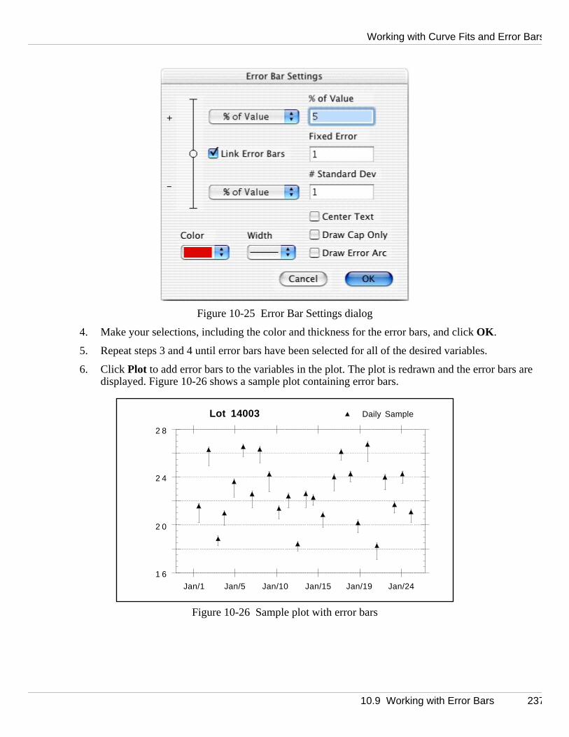
Working with Curve Fits and Error Bars
are
Figure 10-25 Error Bar Settings dialog
4. Make your selections, including the color and thickness for the error bars, and click OK .
5. Repeat steps 3 and 4 until error bars have been selected for all of the desired variables.
6. Click Plot to add error bars to the variables in the plot. The plot is redrawn and the error barsdisplayed. Figure 10-26 shows a sample plot containing error bars.
Figure 10-26 Sample plot with error bars
1 6
2 0
2 4
2 8
Jan/1 Jan/5 Jan/10 Jan/15 Jan/19 Jan/24
Lot 14003 Daily Sample
10.9 Working with Error Bars 237
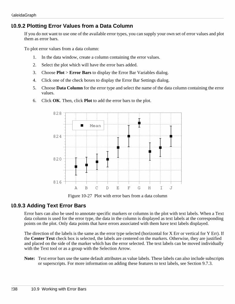
KaleidaGraph
nd plo
erro
a Texponding
Err). Istified vidually
ubscripts3.
10.9.2 Plotting Error Values from a Data ColumnIf you do not want to use one of the available error types, you can supply your own set of error values atthem as error bars.
To plot error values from a data column:
1. In the data window, create a column containing the error values.
2. Select the plot which will have the error bars added.
3. Choose Plot > Error Bars to display the Error Bar Variables dialog.
4. Click one of the check boxes to display the Error Bar Settings dialog.
5. Choose Data Column for the error type and select the name of the data column containing thervalues.
6. Click OK . Then, click Plot to add the error bars to the plot.
Figure 10-27 Plot with error bars from a data column
10.9.3 Adding Text Error BarsError bars can also be used to annotate specific markers or columns in the plot with text labels. Whentdata column is used for the error type, the data in the column is displayed as text labels at the correspoints on the plot. Only data points that have errors associated with them have text labels displayed.
The direction of the labels is the same as the error type selected (horizontal for X Err or vertical for Y fthe Center Text check box is selected, the labels are centered on the markers. Otherwise, they are juand placed on the side of the marker which has the error selected. The text labels can be moved indiwith the Text tool or as a group with the Selection Arrow.
Note: Text error bars use the same default attributes as value labels. These labels can also include sor superscripts. For more information on adding these features to text labels, see Section 9.7.
816
820
824
828
A B C D E F G H I J
Mean
238 10.9 Working with Error Bars

Working with Curve Fits and Error Bars
shows
.
To add text error bars to a plot:
1. In the data window, place the data to be displayed as labels into a Text column. Figure 10-28a sample data set containing a Text column with error values.
Figure 10-28 Sample data set with text errors
2. Select the plot which will have the error bars added.
3. Choose Plot > Error Bars to display the Error Bar Variables dialog.
4. Click one of the check boxes to display the Error Bar Settings dialog, shown in Figure 10-29
Figure 10-29 Error Bar Settings dialog
10.9 Working with Error Bars 239

KaleidaGraph
tex
5. Clear the Link Error Bars check box.
6. Choose None for one of the portions of the bar. For the other, choose Data Column and select the text column containing the labels (in this case Errors ).
7. To center the labels on the marker, select the Center Text check box. Otherwise, the labels are justified.
Note: If the Link Error Bars check box is selected and the Center Text check box is cleared, textlabels are placed on both sides of the marker.
8. Click OK . Then, click Plot to add the labels to the plot. Figure 10-30 shows a sample plot withterror bars added.
Figure 10-30 Plot with text error bars added
0
2
4
6
8
0 2 4 6 8 1 0 1 2 1 4
Test #1
1.4
4.5
5.3
5
3.1
6.8
3.2
6
5 5.2
5
51
.48
3.1
1.7
4
1.5
7
0.5
Ra
ng
e
Time
240 10.9 Working with Error Bars

Working with Curve Fits and Error Bars
You ca
ection oen
ata, the
with
10.9.4 Creating Single-Sided Error BarsSingle-sided error bars are useful when you only want to display the bar on one side of the data point. nchoose a single error type and decide whether to display the positive or negative portion of the bar.
A special case of these error bars results when the errors are taken from a data column. Here the dirfthe error bar is controlled by the sign of the data and whether positive or negative error types have beselected. For positive data, bars are displayed in the same direction as the error type. For negative dbars are displayed in the opposite direction.
To create single-sided error bars:
1. Select the plot which will have the error bars added.
2. Choose Plot > Error Bars to display the Error Bar Variables dialog.
3. Click one of the check boxes to display the Error Bar Settings dialog.
4. Clear the Link Error Bars check box.
5. Choose None for either the positive or negative error type.
6. Choose the type of error to be displayed for the other portion of the bar.
7. Click OK . Then, click Plot to add the error bars to the plot. Figure 10-31 shows a sample plot single-sided error bars added.
Figure 10-31 Plot with single-sided error bars
-0.4
-0.2
0
0.2
0.4
0.6
0.8
1
-2 -1.5 -1 -0.5 0 0.5 1 1.5 2
Sinc(5x)
Sin
c(5x
)
-π/2 to π/2
10.9 Working with Error Bars 241

KaleidaGraph
y the r
pea dialog
10.9.5 Adding Error ArcsError arcs can be displayed instead of error bars. This is done by selecting the Draw Error Arc check box inthe Error Bar Settings dialog. An arc is displayed when one of the error types is set to None. If both positive and negative errors are selected for X Err and Y Err, an ellipse is displayed.
All four quadrants of the ellipse can be controlled independently. The vertical distance is determined bYErr and the horizontal distance is determined by the X Err. This gives you a number of possibilities fodisplaying error arcs and ellipses.
To add error arcs:
1. Select the plot which will have the error arcs added.
2. Choose Plot > Error Bars to display the Error Bar Variables dialog.
3. Click the X Err check box for one of the variables to display the Error Bar Settings dialog.
4. Select the Draw Error Arc check box.
5. Choose the positive and negative error types. Then, click OK . Figure 10-33 shows the dialog containing selections for the X error.
6. Click the Y Err check box for that same variable to define the vertical dimension of the arc. Retsteps 4 and 5 to set up all of the errors of interest. Figure 10-32 shows the Error Bar Settingscontaining selections for the Y error.
Figure 10-32 X error selections
242 10.9 Working with Error Bars

Working with Curve Fits and Error Bars
dded,
Figure 10-33 Y error selections
7. Click Plot to add the error arcs to the plot. Figure 10-34 shows a sample plot with error arcs ausing the settings for the X and Y Error shown above.
Figure 10-34 Plot with error arcs added
0
1
2
3
4
5
6
7
8
0 2 4 6 8 1 0 1 2 1 4
Test #1
Ra
ng
e
Time
10.9 Working with Error Bars 243
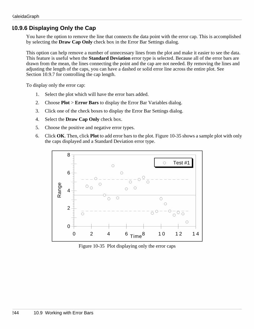
KaleidaGraph
plished
he data. re es and
onl
10.9.6 Displaying Only the CapYou have the option to remove the line that connects the data point with the error cap. This is accomby selecting the Draw Cap Only check box in the Error Bar Settings dialog.
This option can help remove a number of unnecessary lines from the plot and make it easier to see tThis feature is useful when the Standard Deviation error type is selected. Because all of the error bars adrawn from the mean, the lines connecting the point and the cap are not needed. By removing the linadjusting the length of the caps, you can have a dashed or solid error line across the entire plot. SeeSection 10.9.7 for controlling the cap length.
To display only the error cap:
1. Select the plot which will have the error bars added.
2. Choose Plot > Error Bars to display the Error Bar Variables dialog.
3. Click one of the check boxes to display the Error Bar Settings dialog.
4. Select the Draw Cap Only check box.
5. Choose the positive and negative error types.
6. Click OK . Then, click Plot to add error bars to the plot. Figure 10-35 shows a sample plot with ythe caps displayed and a Standard Deviation error type.
Figure 10-35 Plot displaying only the error caps
0
2
4
6
8
0 2 4 6 8 1 0 1 2 1 4
Test #1
Ra
ng
e
Time
244 10.9 Working with Error Bars

Working with Curve Fits and Error Bars
.
10.9.7 Changing the Cap LengthTo change the cap length of error bars:
1. Choose Format > Plot Extras. The dialog in Figure 10-36 is displayed.
Figure 10-36 Plot Extras dialog
2. Edit the value in the Error Bar Length field. A cap is not displayed if zero is entered in this field
3. Click OK to return to the plot.
10.9.8 Removing Error BarsYou can easily remove error bars from individual variables or from all the variables at once.
To remove error bars:
1. Choose Plot > Error Bars . A dialog similar to Figure 10-37 is displayed.
Figure 10-37 Error Bar Variables dialog
2. Clear the check boxes of the error bars to be removed. Clicking Deselect clears all of the check boxesat once.
3. Click Plot to return to the plot window. The plot is redrawn without any error bars.
10.9 Working with Error Bars 245

KaleidaGraph
246 10.9 Working with Error Bars

1Importing and Exporting Graphics
Chapter 11
it an
ption
r layou
u pastever,
This chapter explains how to:
• Import graphics files from other programs into the plot window.
• Print plots.
• Save plots.
• Copy plots to the Clipboard.
• Export plots for use in another program.
• Use Object Linking and Embedding for exporting plots in the Windows version.
11.1 Importing GraphicsKaleidaGraph is able to import a variety of graphic files created in other programs. Choosing File > Import displays a submenu which contains the file formats supported by KaleidaGraph.
When you import a graphic file, the picture is placed in the active plot or layout window. You cannot edyparts of the imported picture. However, you can move and resize the image, and modify its frame.
Note: A plot or layout window must be the frontmost window on the screen. Otherwise, the graphics osare unavailable in the Import submenu.
To import a graphic file:
1. Make the desired plot or layout window the active window.
2. From the File menu, choose Open or the appropriate file type from the Import submenu.
3. Locate and open the file to be imported. The imported image appears as an object in the plot otwindow, with four object handles around it.
11.2 Pasting GraphicsYou can paste graphics cut or copied from other programs into the plot and layout windows. When yoea graphic, it is placed in the active plot or layout window. You cannot edit any parts of the graphic. Howyou can move and resize the image, and modify its frame.
11.1 Importing Graphics 247
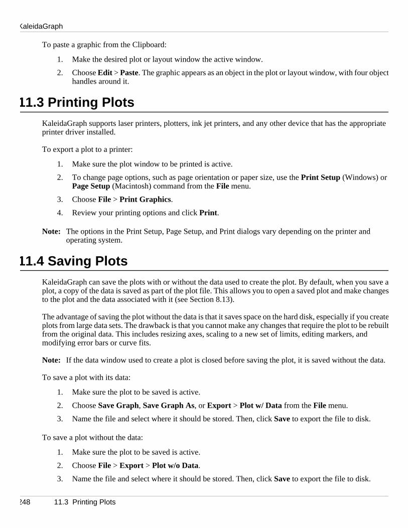
KaleidaGraph
jec
opriate
d
save changes
u create rebuil
data.
To paste a graphic from the Clipboard:
1. Make the desired plot or layout window the active window.
2. Choose Edit > Paste. The graphic appears as an object in the plot or layout window, with four obthandles around it.
11.3 Printing PlotsKaleidaGraph supports laser printers, plotters, ink jet printers, and any other device that has the apprprinter driver installed.
To export a plot to a printer:
1. Make sure the plot window to be printed is active.
2. To change page options, such as page orientation or paper size, use the Print Setup (Windows) or Page Setup (Macintosh) command from the File menu.
3. Choose File > Print Graphics.
4. Review your printing options and click Print .
Note: The options in the Print Setup, Page Setup, and Print dialogs vary depending on the printer anoperating system.
11.4 Saving PlotsKaleidaGraph can save the plots with or without the data used to create the plot. By default, when youaplot, a copy of the data is saved as part of the plot file. This allows you to open a saved plot and make to the plot and the data associated with it (see Section 8.13).
The advantage of saving the plot without the data is that it saves space on the hard disk, especially if yoeplots from large data sets. The drawback is that you cannot make any changes that require the plot to btfrom the original data. This includes resizing axes, scaling to a new set of limits, editing markers, andmodifying error bars or curve fits.
Note: If the data window used to create a plot is closed before saving the plot, it is saved without the
To save a plot with its data:
1. Make sure the plot to be saved is active.
2. Choose Save Graph, Save Graph As, or Export > Plot w/ Data from the File menu.
3. Name the file and select where it should be stored. Then, click Save to export the file to disk.
To save a plot without the data:
1. Make sure the plot to be saved is active.
2. Choose File > Export > Plot w/o Data.
3. Name the file and select where it should be stored. Then, click Save to export the file to disk.
248 11.3 Printing Plots
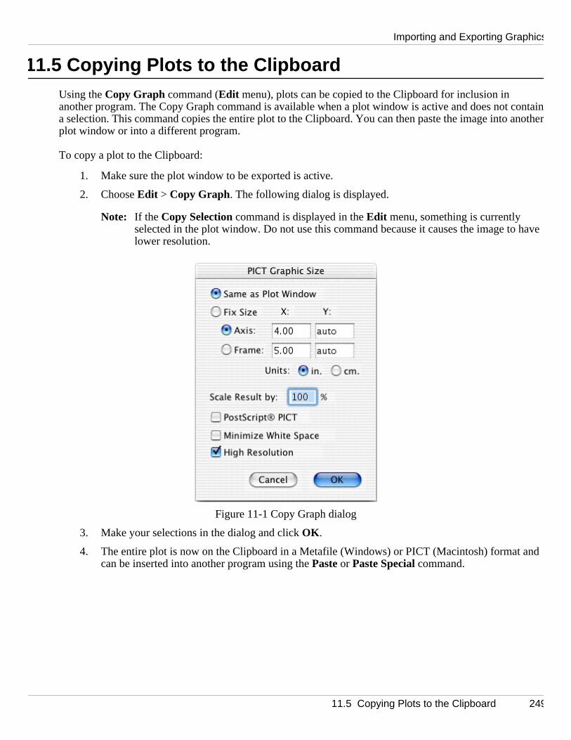
Importing and Exporting Graphics
contain anothe
have
nd
11.5 Copying Plots to the ClipboardUsing the Copy Graph command (Edit menu), plots can be copied to the Clipboard for inclusion in another program. The Copy Graph command is available when a plot window is active and does not a selection. This command copies the entire plot to the Clipboard. You can then paste the image intorplot window or into a different program.
To copy a plot to the Clipboard:
1. Make sure the plot window to be exported is active.
2. Choose Edit > Copy Graph. The following dialog is displayed.
Note: If the Copy Selection command is displayed in the Edit menu, something is currently selected in the plot window. Do not use this command because it causes the image tolower resolution.
Figure 11-1 Copy Graph dialog
3. Make your selections in the dialog and click OK .
4. The entire plot is now on the Clipboard in a Metafile (Windows) or PICT (Macintosh) format acan be inserted into another program using the Paste or Paste Special command.
11.5 Copying Plots to the Clipboard 249

KaleidaGraph
ne o picture.
ye
11.6 Exporting GraphicsKaleidaGraph is able to save plots in a variety of different formats for inclusion in another program. If ofthese files is loaded back into KaleidaGraph, it is treated as a picture. You cannot edit any parts of theHowever, you can move and resize the image within the plot or layout window.
To export a plot for use in another program:
1. Make sure the plot window to be exported is active.
2. Choose File > Export and select the desired file format. A dialog similar to Figure 11-2 is displadto set the size and scaling of the exported file.
Figure 11-2 Set Graphic Size dialog
3. Click OK after making your selections.
4. Name the file and select where it should be stored. Then, click Save to export the file to disk.
250 11.6 Exporting Graphics
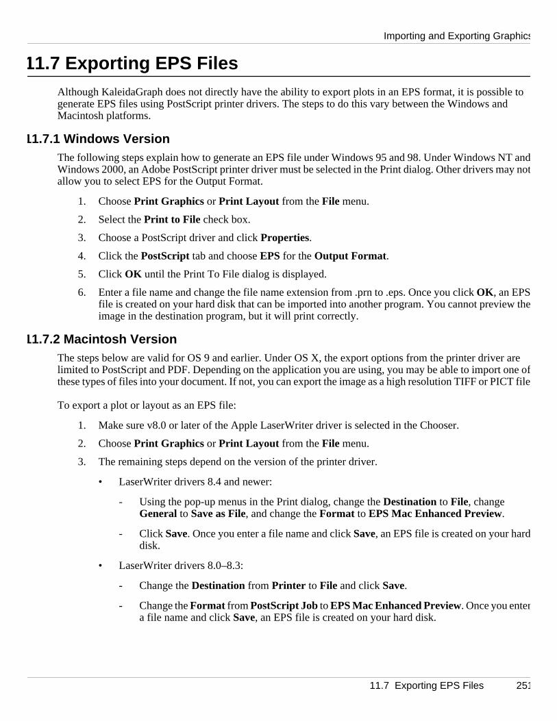
Importing and Exporting Graphics
le to nd
T anay no
ew th
r are one oCT file
11.7 Exporting EPS FilesAlthough KaleidaGraph does not directly have the ability to export plots in an EPS format, it is possibgenerate EPS files using PostScript printer drivers. The steps to do this vary between the Windows aMacintosh platforms.
11.7.1 Windows VersionThe following steps explain how to generate an EPS file under Windows 95 and 98. Under Windows NdWindows 2000, an Adobe PostScript printer driver must be selected in the Print dialog. Other drivers mtallow you to select EPS for the Output Format.
1. Choose Print Graphics or Print Layout from the File menu.
2. Select the Print to File check box.
3. Choose a PostScript driver and click Properties.
4. Click the PostScript tab and choose EPS for the Output Format .
5. Click OK until the Print To File dialog is displayed.
6. Enter a file name and change the file name extension from .prn to .eps. Once you click OK , an EPSfile is created on your hard disk that can be imported into another program. You cannot previeimage in the destination program, but it will print correctly.
11.7.2 Macintosh VersionThe steps below are valid for OS 9 and earlier. Under OS X, the export options from the printer drivelimited to PostScript and PDF. Depending on the application you are using, you may be able to importfthese types of files into your document. If not, you can export the image as a high resolution TIFF or PI
To export a plot or layout as an EPS file:
1. Make sure v8.0 or later of the Apple LaserWriter driver is selected in the Chooser.
2. Choose Print Graphics or Print Layout from the File menu.
3. The remaining steps depend on the version of the printer driver.
• LaserWriter drivers 8.4 and newer:
- Using the pop-up menus in the Print dialog, change the Destination to File, change General to Save as File, and change the Format to EPS Mac Enhanced Preview.
- Click Save. Once you enter a file name and click Save, an EPS file is created on your harddisk.
• LaserWriter drivers 8.0–8.3:
- Change the Destination from Printer to File and click Save.
- Change the Format from PostScript Job to EPS Mac Enhanced Preview. Once you entera file name and click Save, an EPS file is created on your hard disk.
11.7 Exporting EPS Files 251

KaleidaGraph
252 11.7 Exporting EPS Files

2Working with the Layout Window
Chapter 1 2
t labels,
prograys
layout,
s in .
The layout window can be used to place multiple plots on a single page. It can also be used to add texgraphics, or tables to a single plot or to multiple plots on a page. The layout window replaces the Show Pagefeature that was available in earlier versions of KaleidaGraph.
This chapter explains how to:
• Display the layout window.
• Place plots into the layout window.
• Change the size and position of plots in the layout.
• Arrange the plots in the layout window.
• Overlay multiple plots.
• Add a background to the layout.
• Save layout files.
• Export the contents of the layout window.
12.1 Displaying the Layout WindowThe layout window can be displayed using the Show Layout (Windows menu) and New Layout (File menu)commands. The Show Layout command lists any layouts that have been opened or created since themwas started. If a default layout has been saved (in the KG Layout settings file), this submenu will alwacontain an item called KG Layout .
The New Layout command creates an empty layout window. If any changes were made to the current a dialog asks if you want to save the changes before displaying the new layout window.
When the layout window is active, a Layout menu is added to the menu bar. You can use the commandthis menu to place plots in the layout, arrange the plots, and add a background or frame to the layout
12.1 Displaying the Layout Window 253

KaleidaGraph
g the at arindow
and th o
ecausreat
ed to the
12.2 Placing Plots in the Layout WindowYou can place up to 32 different plots in the layout window. Plots are added to the layout window usinSelect Plot command (Layout menu). Choosing this command displays a submenu that lists the plots thecurrently open, from newest to oldest. When you choose a plot from the list, it is placed in the layout w
The name of the plot appears in the lower-left corner of the plot, as shown in Figure 12-2. This is for identification purposes only; it is not included when you print or export the layout.
As plots are added to the layout window, KaleidaGraph maintains a link between the cell in the layout eposition of the plot in the Select Plot submenu. If a particular cell contains the first plot in the list, openingrcreating another plot will cause the cell to display this new plot.
Any time you open, create, or close a plot, it is possible for the plots in the layout to change positions bethe location of the plots in the Select Plot submenu has changed. For this reason, it is best if you open or ceall of your plots before arranging them in the layout window.
It is also possible to use empty cells, shown in Figure 12-3, to organize the layout. These can be addlayout window by choosing Layout > New Position. The empty cells can be replaced at a later time by clicking the cell and choosing a plot from the Select Plot submenu.
Figure 12-3 Empty cell position
Note: If you open several plots in the Macintosh version but find that some of them are not listed in theShowLayout submenu, you need to allocate more memory to the KaleidaGraph program.
Figure 12-1 Select Plot submenu Figure 12-2 Imported plot
254 12.2 Placing Plots in the Layout Window
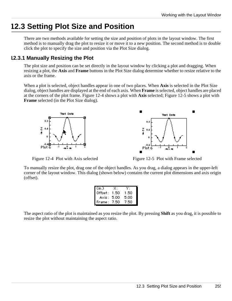
Working with the Layout Window
rst double
en th
er-left origi
12.3 Setting Plot Size and PositionThere are two methods available for setting the size and position of plots in the layout window. The fimethod is to manually drag the plot to resize it or move it to a new position. The second method is to -click the plot to specify the size and position via the Plot Size dialog.
12.3.1 Manually Resizing the PlotThe plot size and position can be set directly in the layout window by clicking a plot and dragging. Whresizing a plot, the Axis and Frame buttons in the Plot Size dialog determine whether to resize relative toeaxis or the frame.
When a plot is selected, object handles appear in one of two places. When Axis is selected in the Plot Size dialog, object handles are displayed at the end of each axis. When Frame is selected, object handles are placedat the corners of the plot frame. Figure 12-4 shows a plot with Axis selected; Figure 12-5 shows a plot withFrame selected (in the Plot Size dialog).
To manually resize the plot, drag one of the object handles. As you drag, a dialog appears in the uppcorner of the layout window. This dialog (shown below) contains the current plot dimensions and axisn(offset).
The aspect ratio of the plot is maintained as you resize the plot. By pressing Shift as you drag, it is possible toresize the plot without maintaining the aspect ratio.
Figure 12-4 Plot with Axis selected Figure 12-5 Plot with Frame selected
12.3 Setting Plot Size and Position 255
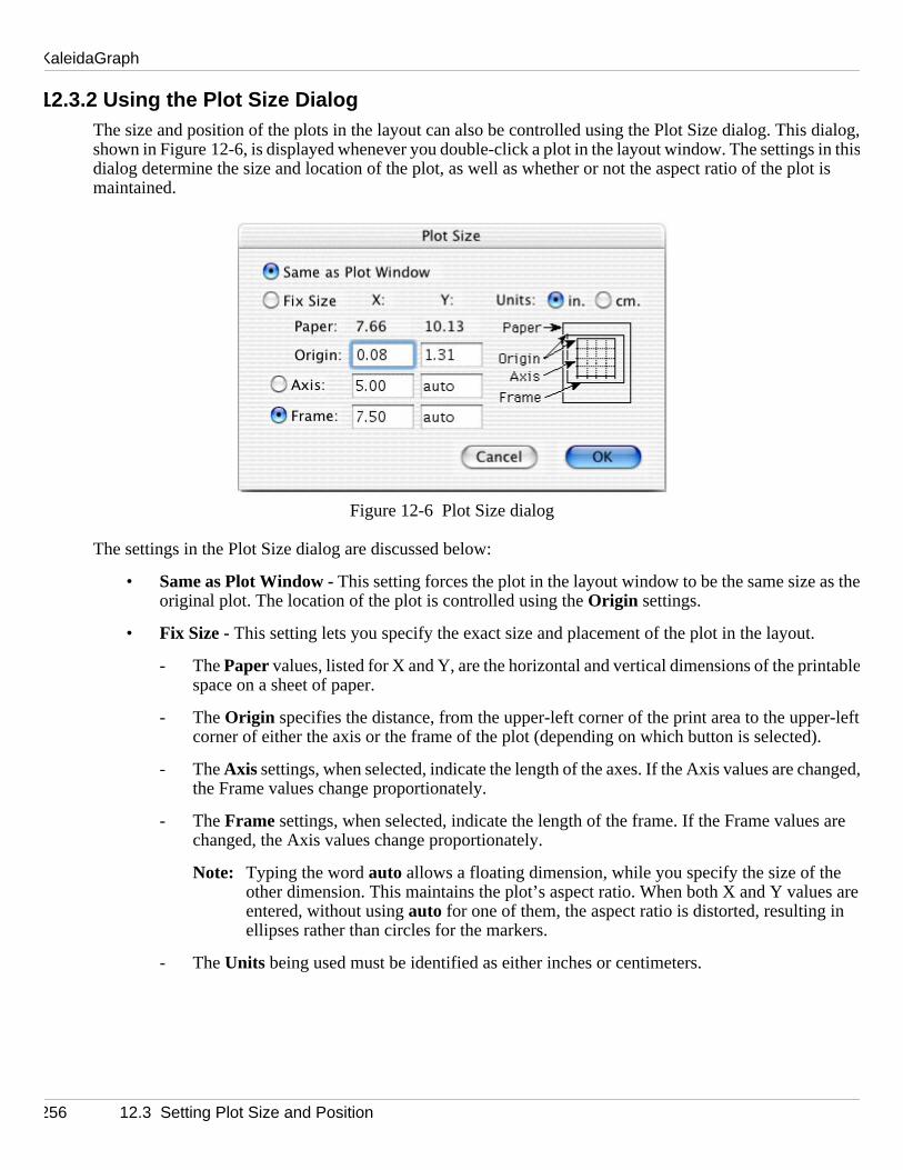
KaleidaGraph
dialog, in thit is
s the
abl
r-left .
nged,
are
s are
12.3.2 Using the Plot Size DialogThe size and position of the plots in the layout can also be controlled using the Plot Size dialog. This shown in Figure 12-6, is displayed whenever you double-click a plot in the layout window. The settingssdialog determine the size and location of the plot, as well as whether or not the aspect ratio of the plomaintained.
Figure 12-6 Plot Size dialog
The settings in the Plot Size dialog are discussed below:
• Same as Plot Window - This setting forces the plot in the layout window to be the same size aoriginal plot. The location of the plot is controlled using the Origin settings.
• Fix Size - This setting lets you specify the exact size and placement of the plot in the layout.
- The Paper values, listed for X and Y, are the horizontal and vertical dimensions of the printespace on a sheet of paper.
- The Origin specifies the distance, from the upper-left corner of the print area to the uppecorner of either the axis or the frame of the plot (depending on which button is selected)
- The Axis settings, when selected, indicate the length of the axes. If the Axis values are chathe Frame values change proportionately.
- The Frame settings, when selected, indicate the length of the frame. If the Frame valueschanged, the Axis values change proportionately.
Note: Typing the word auto allows a floating dimension, while you specify the size of theother dimension. This maintains the plot’s aspect ratio. When both X and Y valueentered, without using auto for one of them, the aspect ratio is distorted, resulting inellipses rather than circles for the markers.
- The Units being used must be identified as either inches or centimeters.
256 12.3 Setting Plot Size and Position

Working with the Layout Window
indow
fect on
pecif
tered.
12.4 Arranging PlotsThe Arrange Layout command (Layout menu) provides a fast and easy way to take the plots and organize them in the layout window. The plots are arranged in the order they were added to the layout w,starting at the top of the page and working down from left to right. When you choose Arrange Layout, the dialog in Figure 12-7 is displayed.
Note: This command can only be used to arrange plots in the layout window. It does not have any afany other objects in the layout window.
Figure 12-7 Arrange Layout dialog
To arrange the plots in the layout window:
1. Place all of the plots in the layout window.
2. Choose Layout > Arrange Layout.
3. Enter the desired number of rows and columns into the Arrange Layout dialog. You can also sythe size of the margin around each of the positions in the layout.
4. Click OK . The layout window is divided equally, based on the number of rows and columns enThe plots are automatically resized and placed into the positions.
12.4 Arranging Plots 257

KaleidaGraph
same
ave the earanc
r the
You n
mplet wit
Figure 12-8 shows a layout window containing five plots in a random pattern. Figure 12-9 shows the layout window after dividing the window into three rows and two columns using the Arrange Layout command.
12.5 Overlaying PlotsYou can use the layout window to position two or more plots on top of each other. These plots must hsame frame and axis dimensions. This is useful if you need to display a single plot with more than themaximum number of variables allowed. By creating separate plots, you can overlay them to get the appeof a single plot.
To overlay two or more plots:
1. Open or create all of the plots that you need to overlay. The plots must be identical in size fomto overlay properly. To ensure that the plots are of equal size, either choose Plot > Define Layout after creating the first plot or use the first plot as a template for creating any remaining plots.can also use the Set Plot Size command (Plot menu) for each plot to make sure the origin, axis, adframe settings are identical.
2. Remove the text labels from all but one of the plots. The following two plots are used in this exa.Figure 12-10 shows a normal plot with all of its labels intact. Figure 12-11 shows a similar ploheverything but the legend deleted.
Figure 12-8 Before choosing Arrange Layout Figure 12-9 After choosing Arrange Layout
0 cm3
4 cm3
8 cm3
Radius
0
90
180
270
-4
0
4
8
0o 5o 1 0o 1 5o 2 0o 2 5o
Pressure
-3
-2
-1
0
1
2
3
.01 .1 1 5
10
20
30
50
70
80
90
95
99
99
.99
9.9
9
Norm(p)
Percent
0
2 0
4 0
6 0
8 0
100
120
140
Jan Feb March
4 0
6 0
8 0
1 0 0
1 2 0
1 4 0
1 6 0
1966 (K) 1967 (K) 1968 (K)
0 cm3
4 cm3
8 cm3
Radius
0
9 0
180
270
- 4
0
4
8
0o
5o
1 0o
1 5o
2 0o
2 5o
Pressure
- 3
- 2
- 1
0
1
2
3
.01 .1 1 5
10
20
30
50
70
80
90
95
99
99
.99
9.9
9
Norm(p)
Percent0
2 0
4 0
6 0
8 0
100
120
140
Jan Feb March
4 0
6 0
8 0
100
120
140
160
1966 (K) 1967 (K) 1968 (K)
258 12.5 Overlaying Plots

Working with the Layout Window
. Thioth th plots
ats.
3. Switch to the layout window.
4. Use the Select Plot command (Layout menu) to import the plots into the layout window.
5. Provided that all of the plots are identical in size, you can use the Align tool to overlay the plotssis done by selecting the plots and using the Align tool to align either the edges or centers in behorizontal and vertical directions. Figure 12-12 shows the result of overlaying the two sample
6. The layout window can then be printed, copied to the Clipboard, or saved in a variety of formYou can also save this layout for future use.
Figure 12-12 Result of overlaying two plots
Figure 12-10 Sample plot Figure 12-11 Second plot with labels removed
0
1
2
3
4
5
6
7
0 2 4 6 8 10 12 14
example #1Test #1
Ra
ng
e
Time
Test #2
example #1Test #2
0
1
2
3
4
5
6
7
0 2 4 6 8 10 12 14
example #1Test #1
Ra
ng
e
Time
12.5 Overlaying Plots 259

KaleidaGraph
owin
frame
an
trolle Stylons.
t wit
12.6 Adding a Background or BorderA background or border can be added to the layout window or to the plots in the layout window. The follgsections explain how to add backgrounds and borders in the layout window.
12.6.1 Adding to the Layout WindowA background can be added to the layout window using the Set Background command (Layout menu). Thisallows you to select a fill pattern for any part of the page not covered by a plot. It also lets you have aaround the entire layout.
Note: Text labels may or may not have the background displayed behind the text. The Erase Background command (in the Format menu of the Edit String dialog) controls what happens. When this commdis turned on, the background is erased.
To add a background or border to the layout:
1. Choose Layout > Set Background. The dialog in Figure 12-13 appears.
Figure 12-13 Set Background dialog
2. Make your selections by clicking the appropriate section of each icon. The background is condby the Color icon and the Fill Pattern portion of the Pattern icon. The border is controlled by theeicon and the Pen Pattern portion of the Pattern icon. Section 9.9 explains the use of these ic
3. Click OK to apply the background or border to the layout window. Figure 12-14 shows a layouha background applied. The text label at the top has Erase Background turned on and the text labelsbelow each plot do not.
260 12.6 Adding a Background or Border

Working with the Layout Window
lisheoolbox
roun of the
Figure 12-14 Sample layout with background
12.6.2 Adding to a Plot in the LayoutIt is possible for each plot in the layout window to have its own background and border. This is accompdby selecting the plot in the layout and using the Color, Pattern, and Style icons from the bottom of the t
The background is controlled by the Color icon and the Fill Pattern portion of the Pattern icon. If a backgdcolor is specified in the original plot window, these settings do not have any affect on the appearanceplot. The border is controlled by the Style icon and the Pen Pattern portion of the Pattern icon.
Note: Any background applied to the layout is also applied to any plots which have None selected for the Fill Pattern and do not have a background color selected in the original plot window.
0
1
2
3
4
5
6
7
0 2 4 6 8 1 0 1 2 1 4
Test #2
Time
Lot 1437-98
Test Results
2
3
4
5
6
7
8
0 2 4 6 8 1 0 1 2 1 4
Test #3
Time
Lot 1437-99
12.6 Adding a Background or Border 261

KaleidaGraph
the
age
to hav
t an
If onicture.
nd
r and
12.7 Exporting the LayoutThe contents of the layout window can be exported by copying the layout to the Clipboard, exporting layout to a file, or printing the layout.
12.7.1 Copying LayoutsTo export a layout to the Clipboard:
1. Make sure the layout window to be exported is active.
2. Choose Edit > Copy Layout. A dialog is displayed to set the size and scaling of the exported im
Note: If the Copy Selection command is displayed in the Edit menu, something is currently selected in the layout window. Do not use this command because it causes the image elower resolution.
3. Make your selections in the dialog and click OK .
4. The entire layout is now on the Clipboard in a Metafile (Windows) or PICT (Macintosh) formadcan be inserted into another program using the Paste or Paste Special command.
12.7.2 Exporting the Layout to a FileKaleidaGraph is able to save layouts in a variety of different formats for inclusion in another program.eof these files is loaded into KaleidaGraph, it is treated as a picture. You cannot edit any parts of the pHowever, you can move and resize the image within the plot or layout window.
Note: For information on saving the layout in an EPS format, refer to Section 11.7.
To export a layout for use in another application:
1. Make sure the layout window to be exported is active.
2. Choose File > Export and select the desired file format. A dialog is displayed to set the size ascaling of the exported file.
3. Click OK after making your selections.
4. Name the file and select where it should be stored. Then, click Save to export the file to disk.
12.7.3 Printing LayoutsTo print a layout:
1. Make sure the layout window to be printed is active.
2. To change page options, such as page orientation or paper size, use the Print Setup (Windows) or Page Setup (Macintosh) command from the File menu.
3. Choose File > Print Layout .
4. Review your printing options and click Print .
Note: The options in the Print Setup, Page Setup, and Print dialogs vary depending on the printeoperating system.
262 12.7 Exporting the Layout

Working with the Layout Window
t file bels o
ased on the
ng any d int
layou
d an
ange do
200, 300,
12.8 Opening and Saving Layout FilesOnce you have created a layout, you can save the organization of the layout for future use. The layoustores the following information: size and position of the cells, the contents and location of any text larobjects, and the background settings.
The plots are not saved as part of the layout file; however, the cells are assigned position numbers bthe order of the plots in the Select Plot submenu. For example, if a cell contains the second plot listed inSelect Plot submenu, the next time you open this layout file, the second plot in the Select Plot submenu willautomatically be loaded into this cell.
Note: To see the position numbers for each of the cells, open the layout file before opening or creatiplots. Any cells that show Position #0 are empty cells and will not automatically have plots loadeothem.
To save a layout file:
1. With the desired layout as the active window, choose Save Layout, Save Layout As, or Export > Layout from the File menu.
2. Give the file an appropriate name and click Save.
To open a saved layout file:
1. Open or create the plots you want to display. There is a precedence for loading plots into thetwindow, as discussed earlier in this section.
2. Use the Open or Import > Layout command (File menu) to open the layout file you saved previously. The plots are automatically positioned according to the layout. The background anytext or graphic elements are also displayed in the layout window.
12.9 Other Layout Window Features
12.9.1 Changing the View of the Layout WindowKaleidaGraph provides several magnification levels for changing the view of the layout window. To chthe magnification of the layout, click the Zoom drop-down menu in the lower-left corner of the layout winwand choose the desired zoom level. The available zoom percentages are: 25, 50, 75, 100, 125, 150, and 400%.
12.9.2 Displaying Rulers and Grids in the Layout WindowTo turn the rulers and grids on and off in the layout window:
1. With the layout window active, choose Plot > Ruler & Grids .
2. Click the appropriate check boxes to display the rulers, grids, or both.
3. Select the proper units that you want to use.
4. Click OK to return to the layout window.
12.8 Opening and Saving Layout Files 263

KaleidaGraph
s started.
he itee
ned off,ntil the
wait a pag
12.9.3 Switching Between LayoutsKaleidaGraph provides a Show Layout command in the Windows menu which can be used to switch betweenthe default KG Layout and any other layouts that have been opened or created since the program waThe active layout is listed first in the submenu. Older layouts are listed below the dotted line.
12.9.4 Deleting Items from the LayoutYou can delete any unwanted items from the layout window in one of two ways. You can either select tmand press Backspace (Windows) or Delete (Macintosh), or select the Eraser from the toolbox and click thunwanted item. These methods work for plots or any other objects you want to delete.
12.9.5 Refreshing the LayoutThe layout window utilizes the Auto Refresh command from the Plot menu. When this command is turnedon, the plots are updated whenever a change is made in the layout window. When Auto Refresh is turthe plots are not updated and are replaced by placeholders in the layout. The plots are not redrawn uAuto Refresh command is turned on again.
Turning this command off allows you to make several changes in the layout window without having tofor the window to update after each change. This is particularly useful when arranging several plots oneor when working with large data sets.
Appendixes
264 12.9 Other Layout Window Features
Command Reference
Appendix A
ted 10
and int
and ph dat
reac
the objec
y
This chapter provides an overview of the commands available in KaleidaGraph. For more detailed information, including the options in the various dialogs, refer to the online help.
A.1 File MenuNewThis command creates a blank data window for entering data. By default, new data windows are creacolumns by 100 rows in size and are named Data 1, Data 2, and so on. To change any of the attributes ofthe data window, use the Column Format command (Data menu).
OpenThis command opens any KaleidaGraph file that has been previously saved. You can also open text Microsoft Excel files. If a plot or layout window is active, this command can import a variety of graphicsothe window.
MergeYou can use this command to combine data from another file with the active data window. This commopens the data file and places it at the current row and column position. Files may be either KaleidaGraafiles, Microsoft Excel files, or text files.
Note: If you exceed the 1000 column limit while merging files, only the number of columns needed to hthe limit is added.
CloseThis command closes the active window. Clicking the close box performs the same function.
Note: If you want to close the window without saving any changes, press Shift while either clicking the closebox or choosing File > Close/NoSave.
Update & ReturnNote: This command is only available in the Windows version of KaleidaGraph.
This command is displayed when editing an embedded OLE object. Choosing this command updatesembedded plot and returns to the source document. If KaleidaGraph was open prior to editing the OLEtor if other files were opened before choosing this command, the source document is not automaticalldisplayed.
A.1 File Menu 265

KaleidaGraph
is
d, use
n. I
raphiut file.
ate, ie name
update
ich
rmat
ow is
s any part o
aphias the
il
lect th. Onl
SaveThis command saves the active data, plot, layout, or plot script window. Depending on which windowactive, a Save Data, Save Graph, Save Layout, or Save Script command is displayed.
• Save Data - This command saves the data as a KaleidaGraph data file. If text format is desirethe Export command.
• Save Graph - This command saves the plot with its data, provided the data window is still opefyou want to save the plot using a different format, use the Export command.
• Save Layout - This command saves the cell positions and background, as well as any text or gcobjects in the active layout window. This command does not save the plots as part of the layoOnly the positions of the cells are saved.
• Save Script - This command saves the active plot script. If a plot is used as the graphic templtis saved at the same time as the plot script file. In the Windows version, the plot has the samas the script, but with a .qpc file name extension. In the Macintosh version, the plot’s file namecontains the first 25 characters of the script’s file name, followed by .plot.
UpdateNote: This command is only available in the Windows version of KaleidaGraph.
This command is displayed when editing an embedded OLE object. Choosing this command sends thedobject to the source document.
Save AsThis command saves a copy of the current data, plot, layout, or plot script window. Depending on whwindow is active, a Save Data As, Save Graph As, Save Layout As, or Save Script As command is displayed.
• Save Data As - This command saves a copy of the data as a KaleidaGraph data file. If text fois desired, use the Export command.
• Save Graph As - This command saves a copy of the plot with its data, provided the data windstill open. If you want to save the plot using a different format, use the Export command.
• Save Layout As - This command saves a copy of the cell positions and background, as well atext or graphic objects in the active layout window. This command does not save the plots asfthe layout file. Only the positions of the cells are saved.
• Save Script As - This command saves a copy of the active plot script. If a plot is used as the grctemplate, it is saved at the same time as the plot script file. In the Windows version, the plot hsame name as the script, but with a .qpc file name extension. In the Macintosh version, the plot’s fename contains the first 25 characters of the script’s file name, followed by .plot.
ImportYou can use this command to open a variety of files from within KaleidaGraph. Use the submenu to seetype of document to be imported. The Open dialog is displayed, no matter which type of file you specifyyfiles that are the same type as what you choose from the submenu are displayed.
266 A.1 File Menu

Command Reference
lect th
mman
e in thisindows,
empty
r
m of
is
saved i
what isnd
ExportYou can use this command to save a variety of files from within KaleidaGraph. Use the submenu to seetype of document to be saved. The Save dialog is displayed, no matter which type of file you specify.
PreferencesYou can use this command to control how various files are handled when you quit the program. This codalso controls some other general settings for the program.
Note: The settings for this dialog are saved as part of the Style file. If you choose Never for the Style, you must manually overwrite the default Style file by choosing File > Export > Style.
Print Setup/Page SetupThis command controls printing options such as paper size and page orientation. The options availabldialog vary depending on which printer is selected and what operating system you are using. Under Wthe Print Setup command is displayed; on a Macintosh, the Page Setup command is displayed.
New LayoutYou can use this command to create new layouts from scratch. Choosing this command displays an layout window. For more information on using the layout window, see Chapter 12.
PrintThis command prints the contents of the active data, plot, or layout window. If the Macro Calculator oFormula Entry window is active, you can print the active macro in the Calculator. Depending on whichwindow is active, a Print Data, Print Graphics, Print Layout , or Print Program command is displayed.
• Print Data - This command prints the entire data set, if a selection does not exist. A maximu15 columns may be printed on a single page.
• Print Graphics - This command prints the contents of the active plot window.
• Print Layout - This command prints the contents of the active layout window.
• Print Bitmap - This command is only available in the Macintosh version of KaleidaGraph. Thcommand prints a bitmapped version of the graph. To print a bitmap, press Shift while choosing thePrint Bitmap command from the File menu.
• Print Program - This command prints the active program in the Macro Calculator.
Recent FilesThis command displays a submenu that lists the last eight data or plot files that have been opened ornKaleidaGraph. You can open a listed file by choosing its file name from the submenu.
Exit/QuitThis command closes the KaleidaGraph program and returns to the desktop. Under Windows, the Exit command is displayed; on a Macintosh, the Quit command is displayed.
KaleidaGraph saves any changes to the default Style, Macros, Script, and Layout files, depending onspecified in the Preferences dialog. If Prompt is selected for any of the items in the Preferences dialog achanges have occurred to those particular items, a dialog is displayed.
A.1 File Menu 267

KaleidaGraph
st nd is
t anto the t is
plo
ted. s) o
he
cted.ows)
pasted a plo
A.2 Edit MenuUndo/RedoThe Undo command causes the data, plot, or layout window to revert to its state prior to issuing the lacommand or operation. If a command or operation cannot be undone, this command is unavailable anamed Can’t Undo. If it is possible to redo an operation, the Undo command changes to Redo.
CutIn the data window, the Cut command removes a data selection and places it on the Clipboard. In the plodlayout windows, the Cut command removes objects, equations, and text labels that have been added original plot. If you cut any part of the original plot, including the labels, titles, or legend, the entire ploplaced on the Clipboard.
• Cut w/Titles - If Shift is pressed, Cut is replaced by Cut w/Titles. This command includes the column titles when you cut a data selection.
CopyIf the data window is active, the Copy command places a copy of the data selection on the Clipboard. If ator layout window is active, the Copy Graph, Copy Selection, or Copy Layout command is displayed.
• Copy w/Titles - If Shift is pressed, Copy is replaced by Copy w/Titles. This command includes thecolumn titles when copying a data selection.
• Copy Graph - This command is available when the plot window is active and nothing is selecThis command copies the contents of the plot window to the Clipboard as a Metafile (WindowrPICT (Macintosh) image. You can then paste the plot into another program.
• Copy Selection - This command is displayed when any object is selected in the plot or layoutwindow. This command copies the selected object to the Clipboard. If you copy any part of toriginal plot, including the labels, titles, or legend, a copy of the entire plot is placed on the Clipboard.
• Copy Layout - This command is available when a layout window is active and nothing is seleThis command copies the contents of the layout window to the Clipboard as a Metafile (Windor PICT (Macintosh) image.
PasteThis command places the contents of the Clipboard into a data, plot, or layout window. When data isinto a data window, the data in the first row determines the column’s format. When data is pasted intotor layout window, the data is placed in a table.
• Paste w/Titles - If Shift is pressed, Paste is replaced by Paste w/Titles. This command includes thecolumn titles when you paste a selection from the Clipboard into a data window.
Note: There is no difference between the Paste and Paste w/ Titles commands when selections are cut orcopied from KaleidaGraph’s data windows (using the Cut, Copy, Cut w/Titles, or Copy w/ Titles command). If the data on the Clipboard is not from a KaleidaGraph data window, Paste and Paste w/Titles operate as described above.
268 A.2 Edit Menu

Command Reference
o fil
ffec
nthe data
ows. ogram.
,
ed.
slightltitles,
t delete
data hanges,
ce to the data file
ClearIn the data window, choose Clear to delete all selected data cells. The cells below the selection shift up tlthe void.
• Clear w/Titles - If Shift is pressed, Clear is replaced by Clear w/Titles. This command deletes thecolumn titles along with the data.
In a plot or layout window, Clear removes the selected item from the window. This command does not atthe contents of the Clipboard. You can also use the Backspace (Windows) or Delete key (Macintosh) to perform the same function.
Binary Mode/Text ModeThis command controls whether the Cut and Copy commands use binary or text format to copy large amousof data to the Clipboard. When copying 10000 cells or less, both a binary and text representation of tare copied to the Clipboard. This occurs regardless of the Binary Mode/Text Mode setting.
Binary Mode is much faster and allows you to quickly move large amounts of data between data windText Mode should be used if you need to copy more than 10000 cells and paste them into another pr
The active mode is listed in the Edit menu and has a check mark in front of it. To switch between modeschoose the mode that is currently active.
Select AllThis command selects all objects in the current window. If a data window is active, Select All makes a data selection that includes all cells containing data. Any empty cells embedded in the data are also includ
DuplicateThis command makes a copy of selected text or objects in a plot or layout window. The copy is placed ybelow and to the right of the original. If you duplicate any part of the original plot, including the labels, or legend, the entire plot is duplicated.
Clear DataThis command clears the contents of an entire data selection. Only the data is removed; the cells are nodas they are with the Clear command. You can also use the Backspace (Windows) or Delete key (Macintosh)to perform the same function.
Paste LinkNote: This command is only available in the Windows version of KaleidaGraph.
This command pastes the contents of the Clipboard in the data window as a linked DDE object. The pasted into KaleidaGraph maintains a reference to the source document so that when the original file cthe changes are reflected in the KaleidaGraph data file.
Create LinkNote: This command is only available in the Windows version of KaleidaGraph.
This command creates a DDE link to data in a source document. The linked data maintains a referensource document so that when the original file changes, the changes are reflected in the KaleidaGraph
A.2 Edit Menu 269

KaleidaGraph
links
e of th
e the s
tents
n a
ve plo
ts to
data and
pdate
Link OptionsNote: This command is only available in the Windows version of KaleidaGraph.
This command controls whether the linked data is updated automatically or manually. By default, neware set to update automatically. This command can also be used to cancel a DDE link.
OLE OptionsNote: This command is only available in the Windows version of KaleidaGraph.
This command is only displayed when editing an embedded OLE object. This command controls somesettings (size, scaling, and resolution) of the embedded object.
Hide Borders/Show BordersNote: This command is only available in the Windows version of KaleidaGraph.
The Hide Borders command hides the borders surrounding linked data under Windows. Once you hidborders, the command changes to Show Borders. Use the Show Borders command to redisplay the border
Edit TextThis command displays KaleidaGraph’s text editing facility. The text editor is useful for editing the conof the Clipboard and other small editing tasks.
A.3 Gallery MenuThe Gallery menu lists the types of plots that can be created in KaleidaGraph. For more information ospecific plot type, see Section 7.1 or refer to the online help.
A.4 Plot MenuAxis OptionsThis command controls the limits, ticks, grids, and labels for the horizontal and vertical axes in the actit
Plot StyleThis command controls the markers, fill patterns, line styles, and colors which are used in various plorepresent the plotted variables.
Auto LinkWhen this command is turned on, the plot automatically updates whenever a value is changed in thewindow. After changing a data value, moving to another cell causes the update to occur. All curve fitserror bars are automatically recalculated. When Auto Link is turned off, the plot is not updated.
Update PlotThis command forces an immediate regeneration of the plot from the original data set. Clicking the UPlot button ( ) in the data window performs the same function.
270 A.3 Gallery Menu

Command Reference
When gain.
ved by
ove
tly
ns) are , and
s r for d to
ie sliced Stac
move
hang
ow cath
Auto RefreshWhen this command is turned on, the plot or layout window is redrawn whenever a change is made. Auto Refresh is turned off, the plot or layout window is not redrawn until this command is turned on a
Display LegendWhen this command is turned on, the legend is displayed in the plot window. The legend can be remoturning off this command or using the Backspace (Windows) or Delete key (Macintosh) when the legend isselected (which also turns off the Display Legend command). The Eraser tool removes the legend permanently, without turning off this command.
Display TitleWhen this command is turned on, the plot title is displayed in the plot window. The plot title can be remdby turning off this command or using the Backspace (Windows) or Delete key (Macintosh) when the title isselected (which also turns off the Display Title command). The Eraser tool removes the plot title permanen,without turning off this command.
Display EquationWhen this command is turned on, the results from curve fits that have closed form solutions (equatiodisplayed in the plot window. This includes the General, Linear, Polynomial, Exponential, LogarithmicPower curve fits. To change the precision of the results, use the Equation Label Format command (Formatmenu).
Error BarsYou can use this command to add horizontal and vertical error bars to all of the Linear plots, as well aProbability, X-Y Probability, Horizontal Bar, and Column plots. Error bars illustrate the amount of errothe plotted data. They normally appear as lines extending from the data points, with caps on either enrepresent the upper and lower values of the spread.
Add ValuesWhen this command is turned on, the numerical values of bars or columns, or the percentage value of psare automatically placed on the plot. This command affects Pie, Horizontal Bar, Stack Bar, Column, ankColumn plots. The values can be removed by turning off this command or using the Backspace (Windows) or Delete key (Macintosh) when the labels are selected as a group. The Eraser tool can be used to reindividual labels.
The values may be moved as a group with the Selection Arrow, or individually with the Text tool. To cethe format of the values displayed, choose Format > Value Label Format.
Extract DataThis command displays the data used to create a saved plot. The Find Data button ( ) in the plot windnalso be used to extract this data. The Extract Data command is unavailable if the data was not saved with eplot or if it was already extracted.
A.4 Plot Menu 271

KaleidaGraph
w plots nd titles,
lot.
to mov
s placeell.
he last
a grou
gle
electio
Define LayoutThis command is used to save the basic characteristics of the current plot as a mini-template. Any neof that type have the same layout as the original. The layout saves the position of the legend, axes, athe default style for the legend, and the size of the axes, frame, and legend.
Each plot type has its own layout. All layouts are saved in the Style file.
Set Plot SizeYou can use this command to specify the exact size and position of the axes or frame for the active p
Ruler & GridsYou can use this command to display a ruler and a grid in the plot and layout windows.
A.5 Data MenuOverwrite ModeWhen this command is selected, cells are automatically selected when you use the mouse or keyboardeto a cell. Typing data into the current cell replaces any existing data.
Insert ModeWhen this command is selected, clicking a cell does not automatically select the cell. Instead, a cursor idin the cell to edit the current value. To select a cell in Insert Mode, you must double-click the active c
Append ColumnsThis command appends the specified number of columns to the data window. If the current cell is in tcolumn of the data window, pressing Right Arrow automatically adds a new column.
Insert ColumnThis command inserts an empty column to the left of the column currently selected.
Delete ColumnThis command removes selected columns from the data window. You can remove a single column or pof columns using this command.
Insert RowThis command inserts an empty row above the row currently selected. A row can be inserted in a sincolumn or a range of columns.
Delete RowThis command removes selected rows from the data window. You can remove an entire row or a data snfrom the data window.
272 A.5 Data Menu
Command Reference
100. I
he las0 rows
o mak
by matio
sort a
sort
This
our
of datexporte
Add RowsThis command adds the specified number of rows to the data window. Rows are added in multiples offthe active cell is in the last row of the data window, pressing the Enter (Windows), Return (Macintosh), or Down Arrow key adds 100 rows to the data window.
Compress RowsThis command compresses a data window to its minimum size by deleting all empty rows that follow ttphysical row of data. Rows are deleted in multiples of 100. A data window will never have less than 10
Go To CellThis command is used to view an exact cell location in the data window. Choosing Go To Cell displays a dialog to enter the row and column numbers of the desired cell. The data window automatically scrolls tethat cell position visible.
Column FormatThis command is used to edit column titles and change the format of any column in the data window.
Posted NoteThis command displays the Posted Note of the active data window. The same result can be obtainedclicking the Posted Note button ( ) in the data window. The Posted Note can be used to store infornabout the active data set.
A.6 Functions MenuAscending SortThis command sorts numeric or text data in ascending order (from low value to high value). You can column, a range of columns, or any data selection.
Descending SortThis command sorts numeric or text data in descending order (from high value to low value). You canacolumn, a range of columns, or any data selection.
Create SeriesThis command fills a selection in a data window with an arithmetic, geometric, or time series of data. command does not generate a series in a Text column.
TransposeThis command converts columns to rows and rows to columns. For example, if a selection contains fcolumns and 128 rows, it contains 128 columns and four rows after transposing the data.
Bin DataThis command provides a Histogram-like binning feature. The Bin Data dialog calculates the number apoints within each bin, based on the number of bins and the specified data range. The results can be din any one of three formats for plotting or for annotating a plot.
A.6 Functions Menu 273

KaleidaGraph
split-
samplariance.
, an
oxon as the
factor.
of three
the dat
is a
rrange th
StatisticsThis command displays the statistics for the frontmost data window. The Statistics dialog provides a screen display so that any two columns within the same data window can be compared.
Student tThis command performs a t-test on selected data. KaleidaGraph provides four types of tests: the singleet-test, the paired t-test, the unpaired t-test with equal variance, and the unpaired t-test with unequal v
ANOVAThis command performs an analysis of variance (ANOVA) for the active data window. KaleidaGraph provides four types of tests: one way ANOVA, two way ANOVA, one way repeated measures ANOVAdtwo way repeated measures ANOVA. In addition, four post hoc tests can be used to determine whichtreatments have an effect or which groups are different.
WilcoxonThis command can be used to perform three nonparametric tests for the active data window: the Wilcsigned rank test, the Wilcoxon matched pairs test, and the Wilcoxon-Mann-Whitney test (also knownMann-Whitney test).
Kruskal-WallisThis command performs a Kruskal-Wallis test to see if three or more groups are affected by a single
FriedmanThis command performs a Friedman test to see if a single group of individuals is affected by a series or more treatments.
MaskThis command masks one or more selected cells. Masked data is not plotted or used in curve fits. In awindow, masked data is shaded (with a stipple pattern) to make it stand out from unmasked data.
UnmaskThis command unmasks any masked data in the selected region of the data window.
A.7 Macros MenuThe Macros menu lists three commands followed by a list of the macros stored in your Macros file. Thsection contains an overview of the macros provided with KaleidaGraph. For more information aboutspecific macro, refer to the online help.
Show MacrosThis command can be used to add new macros to the menu, remove macros already present, and reaemacros. A maximum of 100 macros can be stored in this menu at once.
274 A.7 Macros Menu

Command Reference
stom
aliasesry, refe
ot listed to the
urve
the
asked
n
X-Yformedits.
oints pezoids
ibinnt slope
n place
it. Th
Note: The macros stored in the Macros menu are saved, by default, in a file called KGMacros (Windows) or KG Macros (Macintosh). This file is loaded each time you start KaleidaGraph. To open a cufile, use the Open or Import commands in the File menu.
Edit MacrosYou can use this command to edit macros currently listed in the Macros menu.
LibraryThis command displays the contents of the current library. The library is a place where you can enteror shorthand references for functions, variables, and constants. For more information on using the librarto Section 6.8.
Default MacrosThis section describes the default macros that are supplied with KaleidaGraph. If these macros are nin the Macros menu, see the troubleshooting section in the online help for instructions on adding themmenu.
• Filter - This macro eliminates outliers from a varying curve. It computes a moving-average cwith a user-defined window size as the reference curve for comparison against the data.
• Smooth - This macro computes a moving average of a curve. The resulting column of data isaverage of the n-points surrounding the current data point. In this macro, n must be odd.
• Simplify - This macro masks any consecutive data points that do not differ from the last unmvalue by a certain error. Notice that this is the opposite of what the Filter macro does.
• Invert Mask - This macro masks unmasked data and unmasks masked data in a single data colum
• Integrate - Area - This macro finds the area under a curve, given a lower and upper limit anddata points describing the curve. The area is found by calculating the sum of the trapezoids by the data points and, if necessary, interpolating the points forming the lower and upper lim
• Integral - Curve - This macro finds the incremental area under a curve, given the X-Y data pdescribing the curve. The macro then generates a new curve. The area is the sum of the traformed by the data points and the reference value.
• Derivative - This macro finds the incremental slope of a curve, given the X-Y data points descrgthe curve. The macro then generates a new curve. The slope is calculated using the two-poiformula.
• Series - This macro creates the series: xo, 2*xo, 3*xo, ... (by default, xo=1).
• Unit Series - This macro creates the series: xo, 1+xo, 2+xo, ... (by default, xo=1).
• ππππ Series - This macro creates the series: –π/2, ..., –ε, +ε, ..., +π/2 (where ε=π/(# of selected rows)).
• Sinc (5x) - This macro creates a column containing sin(5x)/(5x).
• abs(x) - This macro takes the absolute value of the selected column and replaces the column i
• Random# - This macro generates a series of random numbers between a lower and upper limeresulting series of numbers is stored in column 0.
A.7 Macros Menu 275

KaleidaGraph
eral cutin
option
ou use
for th
Other MacrosThe following macros are not in the default Macros file, but are stored in the Macro Source folder as text files.You may load these files into the Macro Calculator using either the File > Import > Program Text commandor the Open command in the program editor of the Macro Calculator.
• View General - This macro displays the results of the previous General curve fit.
• View Covariances - This macro displays the covariances of the previous General curve fit.
• Paste Covariances - This macro places the covariance/correlation matrix of the previous Gencurve fit in the selected region of the data window. A group of cells must be selected before exegthis macro.
A.8 Format MenuPlot ExtrasThis command controls the length and thickness of several plot elements. You can also set some of thesassociated with Line and Column plots.
Plot ColorThis command controls the frame, grid, interior, and background colors of the plot. If None is selected for theinterior or background color, that portion of the plot is transparent.
X Label FormatThis command controls the format of the labels on the X axis.
Y Label FormatThis command controls the format of the labels on the Y axis.
Y2 Label FormatThis command controls the format of the labels on the Y2 axis.
X2 Label FormatThis command controls the format of the labels on the X2 axis.
Value Label FormatThis command controls the format of any value labels on the plot. Value labels are displayed when ythe Add Values command (Plot menu) or add text error bars.
Equation Label FormatThis command controls the format and precision of any curve fit equations on the plot.
Text OptionsThis command controls several options associated with text labels, including the default attributes usedevarious labels in the plot window.
276 A.8 Format Menu

Command Reference
are
near o
e edg
layout
dow,
r layou
ow,
Polar OptionsThis command controls the grid type, data format, reference angle, and direction for Polar plots.
Curve Fit OptionsThis command controls several options associated with curve fits, including whether or not curve fits drawn to the axis limits.
Probability OptionsThis command controls the type of distribution used in Probability plots. You can choose between a lirnormal distribution.
Histogram OptionsThis command controls the bin size, reference value, and number of extra bins in a Histogram plot.
Step OptionsThis command controls the placement of the steps when using a Step plot.
A.9 Object MenuAlignYou can use this command to align selected objects in the plot or layout window. When using one of theoptions, objects are aligned by their border centers, regardless of the thickness.
UpThis command moves one or more selected objects forward one level in the object order of a plot or window, changing the draw order of the objects.
Bring To FrontThis command moves one or more selected objects in front of all other objects in a plot or layout winchanging the draw order of the objects.
DownThis command moves one or more selected objects backward one level in the object order of a plot otwindow, changing the draw order of the objects.
Send To BackThis command moves one or more selected objects behind all other objects in the plot or layout windchanging the draw order of the objects.
GroupThis command combines two or more objects into a single object.
UnGroupThis command separates a previously grouped object into its original components.
A.9 Object Menu 277

KaleidaGraph
fferent cted ite
lor file,
lso rese
atiociate
ge fits. A
ry is tol for the y and
pene
click
ty cell
Edit ObjectYou can use this command to edit text, arrows, polygons, Bezier curves, tables, and plot axes. If a ditype of object is selected when you choose this command, a beep sounds to let you know that the selemcannot be edited.
Edit ColorsYou can use this command to edit the colors on the palette, save a custom color file, load a saved coor print the current palette. You can also reset the palette to its original defaults using this command.
Edit Arrow HeadsYou can use this command to customize the height, length, and inset for each arrow style. You can atthe arrowheads to their default settings using this command.
A.10 Curve Fit MenuThe Curve Fit menu lists the types of curve fits that can be applied within KaleidaGraph. For more informnon a specific type of fit, refer to Section 10.1 or the online help. The following two commands are assodwith the General curve fit. See Section 10.5 for more information on the use of these commands.
Edit GeneralThis command can be used to add new fits to the submenu, remove fits already present, and rearranmaximum of 16 curve fits can be stored in this submenu.
LibraryThis command displays the contents of the current library. One of the main reasons for using the libraform aliases or shorthand references for functions, variables, and constants. This is particularly usefudefining sections of a formula that exceed the 256 character limit in the Curve Fit Definition dialog forGeneral curve fit. Section 10.5.7 provides some examples for defining curve fit equations in the librarcalling the definitions from the Curve Fit Definition dialog.
Note: Do not use the library to open text files containing saved curve fit definitions. These should be odfrom within the Curve Fit Definition dialog.
A.11 Layout MenuNew PositionThis command places an empty cell in the layout window. To place a plot into an empty cell position,the cell and select a plot from the Select Plot submenu.
Select PlotYou can use this command to place plots into the layout window. If you want to replace a plot or empin the layout, click the item to be replaced and choose a plot from the Select Plot submenu.
278 A.10 Curve Fit Menu
Command Reference
s and one oe top o
d using
it is
n itebere
e in whe
tation) ate anmore
Entr
Arrange LayoutYou can use this command to arrange the plots in the layout window by specifying the number of rowcolumns you want to have. The layout window is divided into equal sections, with each plot occupying fthe divisions. The plots are arranged in the order they were added to the layout window, starting at thfthe page and working down from left to right.
Set BackgroundYou can use this command to set a background and border for the layout window.
A.12 Windows MenuHide WindowThis command can be used to hide an open window. Hidden data and plot windows can be redisplayethe Show Data and Show Plot commands.
Show DataThis command can be used to bring any data window to the front.
Show PlotThis command can be used to bring any plot window to the front.
Show LayoutThis command brings the selected layout window to the front. Each time you open or create a layout,added to the Show Layout submenu.
If a default layout has been saved (in the KG Layout settings file), this submenu will always contain amcalled KG Layout . It is not possible to permanently add layouts to this submenu. They are only rememduntil you quit the program.
ClipboardThis command displays the Clipboard window, which contains the last item that was cut or copied. Thcontents of the Clipboard remain intact until another selection is cut or copied. The contents also remanswitching between programs. This allows you to easily transfer selections between programs.
Macro CalculatorThis command displays the Macro Calculator. The calculator combines the RPN (Reverse Polish Noprogramming language with support for 1000 program steps to give you a number of ways to manipuldtransform data. Refer to the online help or the Macro Calculator online manual (on the CD-ROM) for information on the Macro Calculator.
Formula EntryThis command displays the Formula Entry window. See Chapter 6 for information on using the Formulaywindow.
A.12 Windows Menu 279

KaleidaGraph
. See
aved
ntain
ese
ve it to
Plot ScriptThis command can be used to create a number of plots at once that all have the same characteristicsSection 7.4.3 for information on using the Plot Script command.
Show All PlotsThis command displays all open plot windows at once.
Hide All PlotsThis command hides all open plot windows at once.
Close All PlotsThis command closes all open plot windows at once. A dialog appears if any of the plots contain unschanges.
Close All DataThis command closes all open data windows at once. A dialog appears if any of the data windows counsaved changes.
Menu ShortcutsThis command can be used to add or change keyboard shortcuts for commands in KaleidaGraph. Thshortcuts are saved as part of the Macros file.
RenameThis command can be used to edit the name of the data, plot, or layout window, without having to sadisk.
280 A.12 Windows Menu
KaleidaGraph’s Settings Files
Appendix B
are ect file
faults,
the differs
aph X or in
g
thrtcuts,
ve the differs
s
KaleidaGraph maintains four settings files to save the modifications made to the program. These filesopened each time you start KaleidaGraph, provided they are in the correct location and have the corrname. If a settings file has a different name or is located in a different directory, the file is skipped.
B.1 Style FilesStyle files contain the settings for most of KaleidaGraph’s dialogs. Any changes made to the original desuch as text attributes, plot layout, and dialog settings, are saved in the Style file.
A default Style file is automatically opened each time KaleidaGraph is started. This way you can savesettings and have them opened the next time you use the program. The name and location of this filebetween the Windows and Macintosh versions of KaleidaGraph.
• Windows: The default settings file is named KGStyle. This file must be in the same directory asKaleidaGraph for it to be opened.
• Macintosh: The default settings file is named KG Style. This file must be in the KaleidaGraph Preferences folder or in the same folder as KaleidaGraph for it to be opened. The KaleidaGrPreferences folder is located in the Preferences folder (in the users Library folder under OS the System Folder for OS 9 and earlier).
Custom Style files can be created by choosing File > Export > Style. These files can be opened by choosinOpen or Import > Style from the File menu. All of the settings change to reflect the contents of the newStyle file.
B.2 Macros FilesMacros files contain the macros in the Macros menu, the contents of the library, any formulas assigned toefunction buttons in Formula Entry, the settings in the Text File Input Format dialog, the keyboard shoand the curve fits in the General submenu.
A default Macros file is automatically opened each time KaleidaGraph is started. This way you can sasettings and have them opened the next time you use the program. The name and location of this filebetween the Windows and Macintosh versions of KaleidaGraph.
• Windows: The default settings file is named KGMacros. This file must be in the same directory aKaleidaGraph for it to be opened.
B.1 Style Files 281
KaleidaGraph
aph X or in
tive lls are
ve a hoosing n
s
aph X or in
ut.
d. This locatio
s
aph X or in
• Macintosh: The default settings file is named KG Macros. This file must be in the KaleidaGraphPreferences folder or in the same folder as KaleidaGraph for it to be opened. The KaleidaGrPreferences folder is located in the Preferences folder (in the users Library folder under OS the System Folder for OS 9 and earlier).
Custom Macros files can be created by choosing File > Export > Macros. These files can be opened by choosing Open, Import > New Macros, or Import > Append Macros from the File menu. All of the affectedmenus and options change to reflect the contents of the new Macros file.
B.3 Layout FilesLayout files contain the cell positions and background, as well as any text or graphic objects in the aclayout window. These files do not save the plots as part of the layout file. Only the positions of the cesaved.
A default Layout file is automatically opened each time KaleidaGraph is started. This way you can salayout and have it opened the next time you use the program. You can access the default layout by cWindows > Show Layout > KG Layout . The name and location of this file differs between the Windows adMacintosh versions of KaleidaGraph.
• Windows: The default settings file is named KGLayout . This file must be in the same directory aKaleidaGraph for it to be opened.
• Macintosh: The default settings file is named KG Layout . This file must be in the KaleidaGraph Preferences folder or in the same folder as KaleidaGraph for it to be opened. The KaleidaGrPreferences folder is located in the Preferences folder (in the users Library folder under OS the System Folder for OS 9 and earlier).
Custom Layout files can be created by choosing Save Layout or Export > Layout from the File menu whena layout window is active. These files can be opened by choosing Open or Import > Layout from the File menu. The layout opens into a new window, displaying any items that were saved as part of the layo
B.4 Script FilesScript files contain the settings and group selections from the Plot Script window.
If one has been created, a default Script file is automatically opened each time KaleidaGraph is starteway you can save the plot script and have it opened the next time you use the program. The name andnof this file differs between the Windows and Macintosh versions of KaleidaGraph.
• Windows: The default settings file is named KGScript . This file must be in the same directory aKaleidaGraph for it to be opened.
• Macintosh: The default settings file is named KG Script . This file must be in the KaleidaGraph Preferences folder or in the same folder as KaleidaGraph for it to be opened. The KaleidaGrPreferences folder is located in the Preferences folder (in the users Library folder under OS the System Folder for OS 9 and earlier).
Custom Script files can be created by choosing Save Script or Export > Script from the File menu when thePlot Script window is active. These files can be opened by choosing Open or Import > Script from the Filemenu. The Plot Script window changes to reflect the contents of the new Script file.
282 B.3 Layout Files

Toolbox Shortcuts
Appendix C
directl
This chapter lists the shortcuts available for selecting plot tools and making changes to plot elements yfrom the toolbox. The online help contains information about the other kinds of shortcuts available in KaleidaGraph.C.1 Shortcuts for Selecting Plot ToolsThe table below lists the keyboard shortcuts available for selecting the various plot tools.
To: Press:
Select the Selection Arrow Spacebar
Select the Text tool T
Select the Line/Arrow tool L
Select the Box tool 1
Select the Rounded-Rectangle tool 2
Select the Oval tool 3
Select the Polygon tool 4
Select the Arc tool 5
Select the Bezier curve tool 6
Activate whatever Object tool is selected in the pop-up menu O
Select the Table tool A
Select the Eraser tool E
Select the Identify tool I
Select the Data Selection tool S
Select the Zoom Selection tool Z
Activate the last tool selected Ctrl (Windows) or (Macintosh)
C.1 Shortcuts for Selecting Plot Tools 283

KaleidaGraph
s
are
C.2 Changing Axis Options from the ToolboxBefore using the toolbox to change the axis options, an axis must be selected by clicking twice on the desired axis. The bottom portion of the toolbox will display the icons shown to the right.
C.2.1 Exchanging and Removing AxesTo exchange or remove axes:
1. Select the desired axis.
2. Click the first Axis Options icon to display the pop-up menu shown below.
3. Turn on Swap X & Y to exchange the X and Y axes or No Axis to remove the selected axis and ittick marks.
C.2.2 Axis Scaling, Reversing, and Auto LimitsTo change scaling, reverse an axis, or return to auto limits:
1. Select the desired axis.
2. Click the second Axis Options icon to display the pop-up menu shown below.
3. Choose Log or Linear to change the axis scaling, turn on Reverse to reverse the axis, or turn on AutoScale to return to the limits originally calculated by KaleidaGraph. The rest of the optionsdiscussed in Sections C.2.4–C.2.6.
C.2.3 Linking AxesTo link the X2 or Y2 axes:
1. Select the X2 or Y2 axis.
2. Click the second of the two Axis Options icons to display the pop-up menu shown below.
284 C.2 Changing Axis Options from the Toolbox
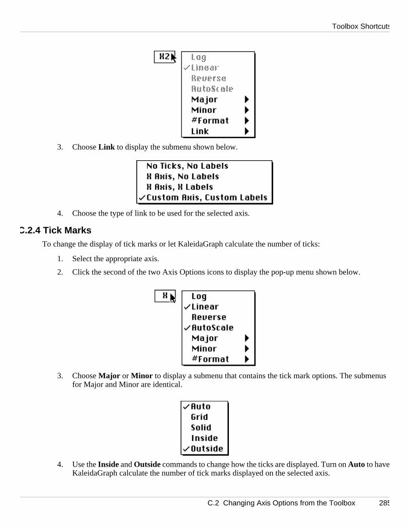
Toolbox Shortcuts
nus
3. Choose Link to display the submenu shown below.
4. Choose the type of link to be used for the selected axis.
C.2.4 Tick MarksTo change the display of tick marks or let KaleidaGraph calculate the number of ticks:
1. Select the appropriate axis.
2. Click the second of the two Axis Options icons to display the pop-up menu shown below.
3. Choose Major or Minor to display a submenu that contains the tick mark options. The submefor Major and Minor are identical.
4. Use the Inside and Outside commands to change how the ticks are displayed. Turn on Auto to haveKaleidaGraph calculate the number of tick marks displayed on the selected axis.
C.2 Changing Axis Options from the Toolbox 285

KaleidaGraph
s fo
men show
C.2.5 Grid LinesTo change how the grid lines are displayed:
1. Select the appropriate axis.
2. Click the second of the two Axis Options icons to display the pop-up menu shown below.
3. Choose Major or Minor to display a submenu that contains the grid line options. The submenurMajor and Minor are identical.
4. Turn on Grid to display a gray (dotted) line or Solid to display a solid line. If both items are turnedoff, grid lines are not displayed.
C.2.6 Axis LabelsTo change the display of the axis labels:
1. Select the desired axis.
2. Click the second of the two Axis Options icons to display the pop-up menu shown below.
3. Choose # Format to display a submenu that contains the display options. The options in the subudepend on the format of the data plotted along the selected axis. The following three figuresthe submenus that appear for Numeric (Float, Double, or Integer), Date, and Time formats.
286 C.2 Changing Axis Options from the Toolbox

Toolbox Shortcuts
eros, abel
Using these options, you can change the format of the axis labels as well as display trailing zcommas, a prefix, or a suffix. Changes are based on the current settings in the appropriate LFormat dialog (Format menu).
4. Make the desired changes to the submenu.
C.3 Changing Plot Style from the ToolboxBefore using the toolbox to change the variable options, a plot symbol must be selected in the legend by clicking twice on the symbol. The bottom portion of the toolbox will display the Plot Style icons shown to the right.
C.3.1 Variable ColorTo change the variable color from the toolbox:
1. Select a plot symbol in the legend.
2. Click the Variable Color icon to display a color palette containing the current color choices.
Numeric formats Date formats Time formats
C.3 Changing Plot Style from the Toolbox 287

KaleidaGraph
3. Select a different color from the palette.
C.3.2 Marker Type, Size, or Number of MarkersTo change the marker type, size, or number of markers displayed:
1. Select a plot symbol in the legend.
2. Click the Marker icon to display the pop-up menu shown below.
3. Select a different marker type, size, or number from the pop-up menu.
C.3.3 Fill PatternTo change the fill pattern of the variable:
1. Select a plot symbol in the legend.
2. Click the Fill Pattern icon to display the pop-up menu shown below.
3. Select a different fill pattern from the pop-up menu.
288 C.3 Changing Plot Style from the Toolbox

Toolbox Shortcuts
. The
dth.
If the nge the
C.3.4 Variable Line Style or WidthTo change the variable’s line style or width:
1. Select a plot symbol in the legend.
2. To change the line style, click the left portion of the Style icon and select a different line styleactive line style is enclosed in a dotted box.
3. To change the line width, click the right portion of the Style icon and select a different line wiThe active line width is enclosed in a dotted box.
C.4 Changing Plot Color from the ToolboxBefore using the toolbox to change the plot colors, either the plot frame or an axis must be selected. frame is selected, you can edit the interior and background colors. If an axis is selected, you can chaframe and grid colors.
C.4.1 Interior and Background Colors
To change the interior or background colors from the toolbox:
1. Click any of the axes once to select the plot’s frame. The bottom portion of the toolbox will display the icons shown to the right.
The Color icon controls the interior and background color. It consists of two sections: an interior color icon (upper left) for setting the plot’s interior color, and a background icon (lower right) for setting the background color.
2. Click one of the icons in the palette to display a color palette containing the color choices.
Line Style pop-up menu Line Width pop-up menu
C.4 Changing Plot Color from the Toolbox 289

KaleidaGraph
splay
rent.
3. Select a different color from the palette.
To make the interior or background of the plot transparent:
1. Click any of the axes once to select the plot’s frame. The bottom portion of the toolbox will ditwo icons.
2. Click the bottom icon to display the following pop-up menu.
3. Turn on either of the commands in this pop-up menu to make that portion of the plot transpa
C.4.2 Frame and Grid ColorsTo change the frame or grid colors from the toolbox:
1. Select one of the plot’s axes. The bottom portion of the toolbox will display the icons shown to the right.
The first icon controls the frame and grid color. It consists of two sections: a frame color icon (upper left) for setting the plot’s frame color, and a grid icon (lower right) for setting the grid color.
2. Click one of the icons in the palette to display a color palette containing the color choices.
3. Select a different color from the palette.
290 C.4 Changing Plot Color from the Toolbox
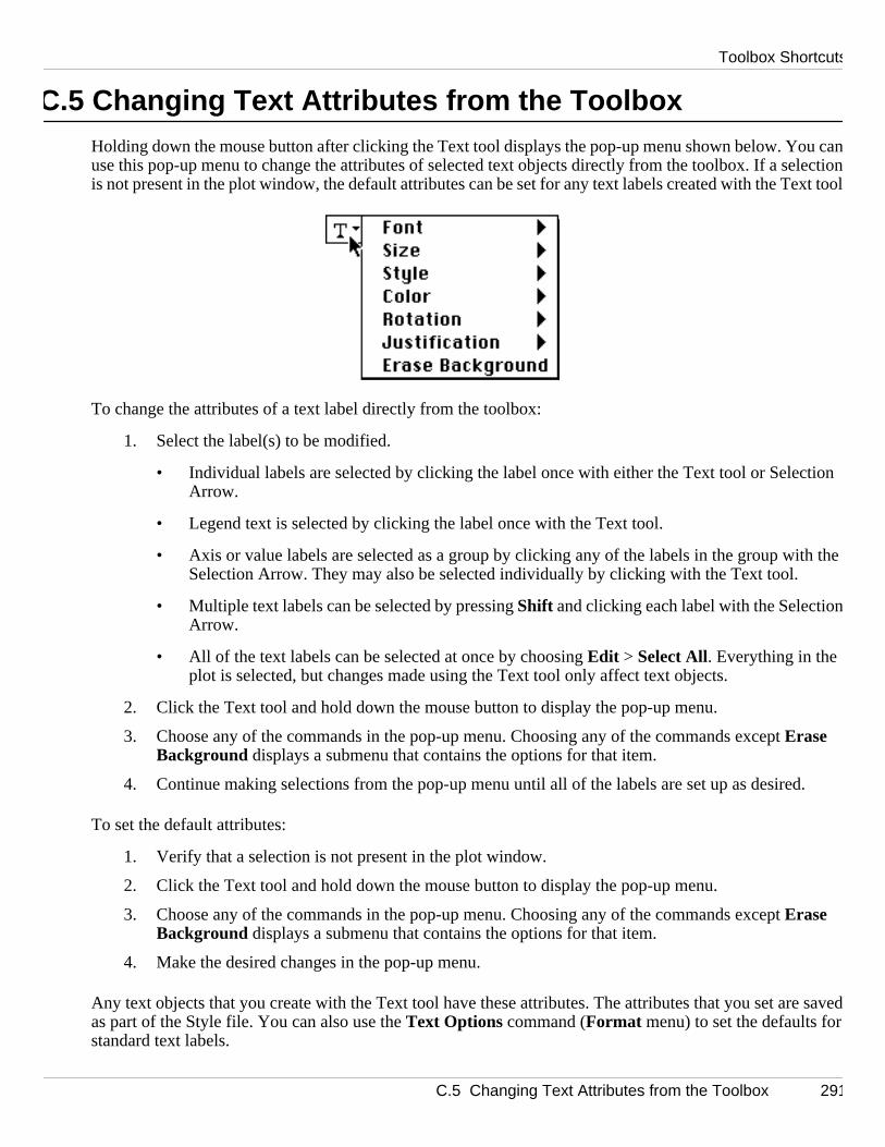
Toolbox Shortcuts
u calectio
ext tool
tion
h the
d.
e save
C.5 Changing Text Attributes from the ToolboxHolding down the mouse button after clicking the Text tool displays the pop-up menu shown below. Yonuse this pop-up menu to change the attributes of selected text objects directly from the toolbox. If a senis not present in the plot window, the default attributes can be set for any text labels created with the T
To change the attributes of a text label directly from the toolbox:
1. Select the label(s) to be modified.
• Individual labels are selected by clicking the label once with either the Text tool or SelecArrow.
• Legend text is selected by clicking the label once with the Text tool.
• Axis or value labels are selected as a group by clicking any of the labels in the group witSelection Arrow. They may also be selected individually by clicking with the Text tool.
• Multiple text labels can be selected by pressing Shift and clicking each label with the SelectionArrow.
• All of the text labels can be selected at once by choosing Edit > Select All. Everything in the plot is selected, but changes made using the Text tool only affect text objects.
2. Click the Text tool and hold down the mouse button to display the pop-up menu.
3. Choose any of the commands in the pop-up menu. Choosing any of the commands except Erase Background displays a submenu that contains the options for that item.
4. Continue making selections from the pop-up menu until all of the labels are set up as desire
To set the default attributes:
1. Verify that a selection is not present in the plot window.
2. Click the Text tool and hold down the mouse button to display the pop-up menu.
3. Choose any of the commands in the pop-up menu. Choosing any of the commands except Erase Background displays a submenu that contains the options for that item.
4. Make the desired changes in the pop-up menu.
Any text objects that you create with the Text tool have these attributes. The attributes that you set ardas part of the Style file. You can also use the Text Options command (Format menu) to set the defaults forstandard text labels.
C.5 Changing Text Attributes from the Toolbox 291
KaleidaGraph
292 C.5 Changing Text Attributes from the Toolbox

Reference Information
Appendix D
m.
and p andptabl
t. You
ata
data
).
This chapter provides information on the methods and equations used in different areas of the progra
D.1 Box Plot DefinitionEach box encloses 50% of the data with the median value of the variable displayed as a line. The topbottom of the box mark the limits of ± 25% of the variable population. The lines extending from the tobottom of each box mark the minimum and maximum values within the data set that fall within an acceerange. Any value outside of this range, called an outlier, is displayed as an individual point.
Note: Outliers are used in the calculations for the Box plot. Removing outliers changes the entire plodo not have any control over the marker used to represent outliers.
Figure D-1 Box plot terms
• Median - The data value located halfway between the smallest and largest values.
• Upper Quartile (UQ) - The data value located halfway between the median and the largest dvalue.
• Lower Quartile (LQ) - The data value located halfway between the median and the smallest value.
• Interquartile Distance (IQD) - The distance between the Upper and Lower Quartiles (UQ - LQ
• Outliers - Points whose value is either:
greater than UQ + 1.5 * IQD or less than LQ - 1.5 * IQD
Upper Quartile (UQ)
Median
Lower Quartile (LQ)
Outlier
Interquartile Distance (IQD)
D.1 Box Plot Definition 293

KaleidaGraph
D.2 Statistics Equations
D.3 Student t-Test Equations
t value (single sample)
t value (paired data)
n = number of data points
xi = current data value (from 1 to n)
= mean of the data
Mean RMS (Root Mean Square)
Standard Deviation Standard Error Variance
Skewness Kurtosis
= mean of the data N = number of data points xi and yi = current data value (from 1 to N)
x x1n--- xi
i 1=
n
∑= 1n--- xi
2
i 1=
n
∑1 2/
xi2
i 1=
n
∑ n x( )2–
n 1–----------------------------------
Standard Deviation
n
---------------------------------------------- xi2
i 1=
n
∑ n x( )2–
n 1–----------------------------------
1n--- xi x–( )3
i 1=
n
∑
1n--- xi x–( )2
i 1=
n
∑ 3 2/----------------------------------------------
1n--- xi x–( )4
i 1=
n
∑
1n--- xi x–( )2
i 1=
n
∑ 2----------------------------------------- 3–
x
tx Test Value–
Standard Error x ( ) -------------------------------------------=
txA xB–
sD-----------------=
sDVar xA( ) Var xB( ) 2Cov xA xB,( )–+
N----------------------------------------------------------------------------------------=
Cov xA xB,( ) 1N 1–------------- xAi
xA–( ) xBixB–( )
i 1=
N
∑≡
294 D.2 Statistics Equations
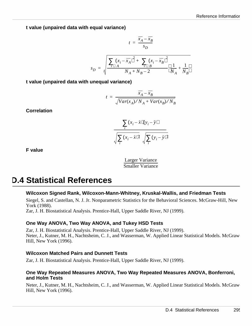
Reference Information
New
Graw
Graw
t value (unpaired data with equal variance)
t value (unpaired data with unequal variance)
Correlation
F value
D.4 Statistical References
Wilcoxon Signed Rank, Wilcoxon-Mann-Whitney, Kruskal-Wallis, and Friedman Tests
Siegel, S. and Castellan, N. J. Jr. Nonparametric Statistics for the Behavioral Sciences. McGraw-Hill,York (1988).Zar, J. H. Biostatistical Analysis. Prentice-Hall, Upper Saddle River, NJ (1999).
One Way ANOVA, Two Way ANOVA, and Tukey HSD Tests
Zar, J. H. Biostatistical Analysis. Prentice-Hall, Upper Saddle River, NJ (1999).Neter, J., Kutner, M. H., Nachtsheim, C. J., and Wasserman, W. Applied Linear Statistical Models. Mc-Hill, New York (1996).
Wilcoxon Matched Pairs and Dunnett Tests
Zar, J. H. Biostatistical Analysis. Prentice-Hall, Upper Saddle River, NJ (1999).
One Way Repeated Measures ANOVA, Two Way Repeated Measures ANOVA, Bonferroni, and Holm Tests
Neter, J., Kutner, M. H., Nachtsheim, C. J., and Wasserman, W. Applied Linear Statistical Models. Mc-Hill, New York (1996).
txA xB–
sD-----------------=
sD
xi xA–( )2
xi xB–( )2
i B∈∑+
i A∈∑
NA NB 2–+-------------------------------------------------------------------------- 1
NA------- 1
NB-------+
=
txA xB–
Var xA( ) NA⁄ Var xB( ) NB⁄+-------------------------------------------------------------------------=
xi x–( ) yi y–( )i
∑
xi x–( )2
i∑ yi y–( )2
i∑
---------------------------------------------------------------
Larger VarianceSmaller Variance-----------------------------------------
D.4 Statistical References 295

KaleidaGraph
D.5 Curve Fit References
General Curve Fit
Press, W. H., Flannery, B. P., Teukolsky, S. A., and Vetterling, W. T.
Numerical Recipes in C.
Cambridge University Press, New York (1988).
Linear, Polynomial, Exponential, Logarithmic, and Power Curve Fits
Beyer, W. H.
Standard Mathematical Tables
. CRC Press, Cleveland (1976).
Smooth Curve Fit
Stineman, R. W. A consistently well-behaved method of interpolation.
Creative Computing
, July (1980).
Weighted Curve Fit
Chambers, J. M., Cleveland, W. S., Kleiner, B., and Tukey, P. A.
Graphical Methods for Data Analysis
. Duxbury Press, Boston (1983).
Cubic Spline Curve Fit
Press, W. H., Flannery, B. P., Teukolsky, S. A., and Vetterling, W. T.
Numerical Recipes in C.
Cambridge University Press, New York (1988).
Interpolate Curve Fit
Stineman, R. W. A consistently well-behaved method of interpolation.
Creative Computing
, July (1980).
296 D.5 Curve Fit References

Reference Information
D.6 Pearson’s R and Chi Square Equations
Pearson’s R (Least Squares curve fits)
Pearson’s R (General curve fit)
Chi Square
χ
2
= Chi Square y
i
= actual value x
i
= calculated value
σ
i
= weight = mean of actual values = mean of calculated valuesy x
R
xi x–( ) yi y–( )i
∑
xi x–( )2
i∑ yi y–( )2
i∑
---------------------------------------------------------------=
R 1 χ2
σi yi y–( )2
i∑--------------------------------–=
χ2yi xi–
σi--------------
2
i∑=
D.6 Pearson’s R and Chi Square Equations 297

KaleidaGraph
298 D.6 Pearson’s R and Chi Square Equations

Glossary
ay
ngengment.
he tick
cesses
ogra
m thhe first
ancho
r false
il the
active window: The frontmost window on the desktop. The active window’s title bar is highlighted.
Align tool: A tool used to align a group of selected objects in the plot or layout window.
analysis of variance (ANOVA): A statistical test that compares the means of two or more groups for astatistically significant difference. KaleidaGraph provides four ANOVA tests: one way, two way, one wrepeated measures, and two way repeated measures.
anchor point: An endpoint on a segment of a Bezier curve. Anchor points contain direction points and tatlines. The position of the anchor points and their direction points determine the shape of the curve se
anchor tick: The anchor tick specifies the value from which all other major tick marks are calculated. Wnplacing major ticks at a specific interval, the interval is counted from the value of the anchor tick. Thisdoes not have to be at the edge of the axis; it can be placed anywhere.
AppleScript: A system-level scripting language available on the Macintosh. It is used to automate prowithin programs that support AppleScript.
Apple Event: A system-level command sent between programs. The command tells the destination prmto perform a specific operation.
Arc tool: A tool used to draw arcs in the plot or layout window.
axis: One of the horizontal or vertical lines in a plot along which values or categories are plotted.
axis labels: Labels that display the values associated with the major tick marks on the plot.
axis titles: Titles that are used to identify which variable is plotted along an axis. The titles are taken froecolumn names being plotted. If multiple variables are plotted on the same axis, the title comes from tcolumn being plotted.
background color: The color KaleidaGraph uses to represent white pixels in fill and pen patterns.
Bezier curve: A curve made up of one or more segments. Each segment is defined by four points: two rpoints, which determine the endpoints, and two direction points, which determine its shape.
Boolean: A value that results from evaluating an expression. The value can be either true (non-zero) o(zero).
Box tool: A tool used to draw squares and rectangles in the plot or layout window.
cell: The basic unit of a data window where values are entered and stored.
Clipboard: A window that contains the last selection that was cut or copied. The contents remain untnext time you cut or copy a selection.
299
KaleidaGraph
lum
he bers
ntosh
The closel
s.
is.
the
t.
menwindow
plot or
ws are
column: In the data window, a vertical line of cells. A maximum of 1000 columns are available. In a conplot, columns are the vertical bars that represent the data values.
column title: The name identifying a column in the data window.
column numbers: The numbers located to the left of the column titles, used to identify each column. Tcolumn numbers are used by Formula Entry and the Macro Calculator during calculations. These numchange when a selection is made in the data window.
Command key: This key ( ) enables you to use keyboard shortcuts to choose commands on a Macicomputer.
comments: Notes added to a macro or function to make it easier to follow.
Ctrl key: This key enables you to use keyboard shortcuts to choose commands under Windows.
curve fitting: The process of applying one of 10 different types of fits to a variable in the plot window.fits can be used to find an equation for the data, to smooth the curve between the points, or to see howythe data compares to a specific equation.
Data Selection tool: A tool used to select a portion of the data on a plot for further plotting and analysi
data window: A window containing a spreadsheet used to enter and store data for plotting and analys
default settings: Settings that KaleidaGraph uses unless you specify different settings. You can save current settings as default settings by choosing File > Export > Style.
degrees of freedom: This is a measure of the sample size, which affects the power of the statistical tes
delimiter: A character used to separate data within a text file; for example, tabs, spaces, or commas.
Dynamic Data Exchange (DDE): A feature that is used to create a link between data in a source docutand a KaleidaGraph for Windows data window. If the data in the source document changes, the data updates to reflect the changes.
Eraser tool: A tool used to delete text and other objects (such as lines, boxes, and pictures) from the layout window.
error bars: Vertical or horizontal lines on a plot that illustrate the statistical error of the data.
extract: To retrieve the original data from a plot which was saved with data. You can use either the Extract Data command or the Find Data button ( ) to display the plot’s data.
fill pattern: A pattern chosen from the pattern palette to fill a selected object.
Find Data button: This button ( ) is located in the upper-right corner of the plot window. Clicking thisbutton displays data windows referenced by the plot. If the data is archived in the plot, the data windoextracted and displayed.
300
Glossary
ay its
enerat
active
n
e curv m4.
e of the
re
.
bels.
layers,
hic
s maty of
t.
foreground color: The color KaleidaGraph uses to represent black pixels in fill and pen patterns.
format: How the data in a column is displayed. Each column has its own format, which controls the wvalues are displayed and used in a plot.
formula: A sequence of values, column references, memory references, functions, or operators that gedata from existing data.
Formula Entry: A window that is used to enter and execute algebraic formulas which operate on the data window.
formula script: A program written in the Posted Note of the Formula Entry window. Formula scripts caautomate the process of opening data, creating plots, and exporting plots to disk or to a printer.
frame: The line surrounding a bar, column, pie wedge, legend, or object in the plot or layout window.
Gaussian equation: An equation of the form m1+m2*exp(–(m0–m3)*(m0–m3)/(m4*m4)). A good startingvalue for m1 is the value that the tails of the curve approach for large values of |x|. The maximum of thecan be used for m2. The mean of the data is a good guess for m3. The bell-width is a good guess for
grid lines: Horizontal or vertical lines that may be displayed at the major and minor tick marks.
group: To combine two or more objects so that they act as a single object.
handles: Points at the corners of an object’s boundary which can be used to modify the size and shapobject.
Home button: This button ( ) is located in the upper-left corner of the data window. Click this button toreturn the data window to its origin (row 0, column 0).
Identify tool: A tool used to find coordinates of points on a plot.
indexed data: A type of data format where a factor column contains the group names, and one or mocolumns contain the corresponding data values for each group.
insertion point: The blinking vertical line that appears whenever you click within a cell or a text dialog
justification: The method used to align text and labels. You can left, center, or right justify text and la
layer: A separate part of the plot window used to organize objects. You can create plots with several with each layer containing different objects.
Layout file: A settings file that contains the cell positions and background, as well as any text or grapobjects in the active layout window.
Layout window: A window used to place multiple plots on a single page. Text, tables, and other objectybe placed anywhere in the layout window. The page may be copied to the Clipboard, saved in a varieformats, or printed.
legend: The portion of the plot that contains symbols and labels used to identify each variable in a plo
301

KaleidaGraph
les.
the
dialog,
ms.
peratd
ragging
ows make
single
f thereel
lly
s.
le plot
library: Used to create and store shorthand references for functions, curve fits, constants, and variab
Line/Arrow tool: A tool used to add lines or arrows to the plot or layout window.
macro: An RPN program that performs a series of calculations on the active data window.
Macro Calculator: An RPN calculator which can be used to write and execute macros that operate onactive data window.
Macros file: A settings file that contains the macros in the Macros menu, the contents of the library, any formulas assigned to the function buttons in Formula Entry, the settings in the Text File Input Format the keyboard shortcuts, and the curve fits in the General submenu.
major ticks: Marks that display the major divisions along an axis.
marker: A symbol which represents a single data point in the plot window.
Metafile: A Windows file format used by graphics programs to transfer documents to different progra
minor ticks: Minor ticks display the divisions between the major tick marks.
nonparametric tests: Statistical tests that do not require the data be normally distributed. These tests oeon the ranks of the values. Examples of nonparametric tests include the Wilcoxon, Kruskal-Wallis, anFriedman tests.
object handles: Small squares that appear when an object is selected. The object can be resized by dthese handles.
Object Linking and Embedding (OLE): A feature that can be used to embed a KaleidaGraph for Windplot in another application. To edit an embedded plot, double-click the plot to start KaleidaGraph andchanges.
Oval tool: A tool used to draw circles and ovals in the plot or layout window.
overlay: To place multiple plots on top of each other in the layout window to get the appearance of a plot.
P value: This value is a probability, with a value that ranges from zero to one. It is used to determine iis a statistically significant difference in the groups being analyzed. If this value is below a certain lev(usually 0.05), the conclusion is that there is a difference between the groups.
parametric tests: Statistical tests that assume the samples are drawn from populations that are normadistributed. Examples of parametric tests include the t-test and analysis of variance (ANOVA).
pen pattern: A pattern given to the line segments of an object.
PICT: A Macintosh file format used by graphics programs to transfer documents to different program
plot script: A series of data selections from any number of data windows that are used to create multipsat once. A plot script is created in the Plot Script window.
302

Glossary
ery
etweethe
it is line
umns.
ject’s
ts
me fo
ade to.
istics as
yout
plot title: The name of the graph. By default, its name is taken from the name of the data window.
plot window: Any window that contains a plot. Plots are created by choosing a plot type from the Gallmenu. When the plot window is active, certain menus are displayed that only affect the plot window.
Polygon tool: A tool used to draw an object with any number of sides in the plot or layout window.
post hoc tests: Post hoc tests (also known as multiple comparisons) are used to isolate the differences bngroups when performing a one way or one way repeated measures ANOVA. KaleidaGraph provides following post hoc tests: Tukey HSD, Bonferroni, Holm, and Dunnett.
Posted Note: A text editor available in both the data and Formula Entry windows. In the data window, used to enter information about the current data set. In Formula Entry, it can be used to write a multi-formula or a script to automate the plotting process.
raw data: A type of data format where the data values for each group are placed in separate data col
residual: The difference between an actual data value and a mean or other estimated value.
Rounded Rectangle tool: A tool used to draw squares and rectangles which have rounded corners.
row: A horizontal line of cells. A maximum of 1 million rows can be displayed in the data window.
row numbers: The column of numbers that appear on the left side of every data window.
Script file: A settings file that contains the settings and group selections from the Plot Script window.
Selection Arrow: A tool used to select, move, and resize objects. This tool is also used to select an obproperties from pop-up menus.
shift-click: To click the mouse button while pressing Shift. This technique is used to select multiple objecor deselect individual objects.
sort key: A column that contains the values you want to sort by. You can specify three sort keys at a tireach sort.
Style file: A settings file that contains the settings for most of KaleidaGraph’s dialogs. Any changes mthe original defaults, such as text attributes, plot layout, and dialog settings, are saved in the Style file
Table tool: A tool used to create tables of data within the plot or layout window.
template: Any plot that is used as a base for creating new plots. The new plot has the same characterthe template.
Text tool: A tool used to create and edit labels in the plot or layout window.
tick marks: The lines which indicate the major or minor increments along an axis.
toolbox The floating window which displays the tools available to create and edit items in the plot or lawindow.
303

KaleidaGraph
ungroup: To separate a grouped object into its original components.
Update Plot button: This button ( ) is located in the upper-right corner of the data window. Click thisbutton to force an immediate update of the plot that is currently linked to it.
X axis: The horizontal axis in a plot, which usually represents the independent variable.
Y axis: The vertical axis in a plot, which usually represents the dependent variable.
Zoom Selection tool: A tool that can be used to quickly change the axis limits.
304

Index
Symbols! 105- 105!= 106#CLEAR command 112#CLEARDATA command 112#CLOSE command 113#CLOSE/ALL command 113#CLOSE/OPT command 113#COPY command 113#CUT command 114#DATA command 114#DATA/NOTITLE command 114#DATAFILE command 115#FORMULA command 115#MERGEFILE command 116#METAFILE command 116#METAFILE/OPT command 116#OPEN command 117#PAGE_PRINT command 117#PASTE command 117#PICT command 118#PICT/OPT command 118#PLOT_PRINT command 118#SAVE command 118#SCRIPT command 119#SELECTION command 120#SET_DIRECTORY command 121% 105&& 106( ) 105* 105+ 105/ 105< 105<= 105= 106== 106> 105
>= 105? : 106[ ] 98, 106^ 105|| 106π Series macro 275
Numerics0o Rotation command 198180o Rotation command 198270o Rotation command 19890o Rotation command 198
Aabs() function 106abs(x) macro 275active window, changing 39, 147Add Rows command 42, 273Add Values command 170, 175, 271Add Windows file extensions check box 17adding
background or border to a layout 260comments to a formula script 112comments to formulas 97curve fits to Curve Fit menu 219curve fits to saved plots 220data to saved plot 168empty cells to a layout 254error bars 236–245lines to Bar/Column plots 171plots to a layout 254rows and columns 42subscripts and superscripts to text 197value labels 170, 175
Align command 192, 277Align tool
description 179using 192
aligning objects 192All Windows check box 45Allowable Error field 217
305
KaleidaGraph
Alpha pop-up menu 89Alt. Font command 184alternate font 44analyzing data
one sample 71–73repeated measurements 82–88two or more groups 74–81
Anchor Tick field 152, 157angular axis 172annotating markers 238ANOVA
one way 78one way repeated measures 85reference 295two way 80two way repeated measures 86
ANOVA command 79, 80, 86, 87, 274Append Columns command 42, 272applying
Cubic Spline curve fit 213–214General curve fit 224–225Polynomial curve fit 211–213
Arc tooldescription 178using 201
arcscreating 201editing 202error arcs 242
Arrange Layout command 257, 279arranging plots 257arrowheads, editing 201arrows
creating 200editing 201
Ascending Sort command 59, 273ASCII files, importing 50–57aspect ratio 255assigning formulas to function buttons 95Auto Link command 167, 270Auto Print check box 145Auto Refresh command 264, 271Auto Save check box 145Automatically dispose of old plots check box 146, 148automating 111–124, 140–146axes
306
editing 152–155exchanging 153, 284linking 154, 284
axisangular 172hiding 153, 284limits 152, 187linking a second axis 154radial 172removing 284resizing 165–166reversing 153, 284scaling 284thickness 155
axis labelsdescription 15editing 159–160, 196formatting 160, 286frequency 160removing 160reversing 153, 284
axis limitssetting 152Zoom Selection tool 187
Axis Options command 152–160, 270Axis settings
Plot Size dialog 256Set Plot Size dialog 165
axis titlesdescription 15editing 196
Bbackground
adding to a layout 260color
editing plot color 164, 290legend 149objects 205–206
Bar charts 130–132, 169–171Bezier curve tool
description 178using 203–204
Bezier curvescreating 203description 203editing 204
Bin Data command 66, 273

Index
Binary Mode command 58, 269binning data 66–68Black Column Frame check box 169Bonferroni test 89, 295border 260Box plot
definition 293description 129
Box tooldescription 178using 201
break 49Bring To Front command 193, 277buttons
Find Data button 14, 137, 167–168Home button 12, 40Posted Note button 46, 96, 111, 273Update Plot button 12, 167–168, 270
Ccalculating
curve fit values 100–103statistics 65, 97–98with date and time data 103
Can't Undo command 268canceling
General curve fit 225Cell Background command 183Cell Horizontal Line command 183Cell Vertical Line command 183cell() function 94, 106cells
entering data into 47moving between 40referencing in formulas 94selecting 41
Center Justification commandEdit String dialog 198Edit Table dialog 183
Center Text check box 238changing
axis limits 152, 187axis scaling 153, 284axis thickness 155cap length 245color of legend text 151
column width 45data format 45display of tick marks 156fill and pen patterns 149, 206foreground and background color 149, 205grid line thickness 158line styles and widths 150, 207magnification 148, 263marker thickness 163number of tick marks 156plot color 164, 289plot lines, markers, and fill patterns 161tick mark interval 157tick mark length and thickness 157
Chi Square 231Chi Square equation 297choosing
post hoc test 89statistical test 70
circlescreating 201editing 202
Clear command 58, 191, 269Edit String dialog 197Edit Table dialog 182
Clear Data command 58, 269Clear w/Titles command 269clearing data 58Clipboard 58, 185, 191, 249, 262Clipboard command 279Close All Data command 40, 280Close All Plots command 148, 280Close command 40, 148, 265
Edit Table dialog 182Close/NoSave command 40, 148, 265closing
data windows 40plot windows 148
cmax() function 108cmin() function 108Coefficient of Determination 231color
background 164, 205–206, 289curve fit 163customizing 278error bars 237foreground 205–206
307
KaleidaGraph
grid line 164, 290interior 164, 289legend text 151plot frame 164, 290text 198variable 163, 287
Color icon 149, 205, 260toolbox 179–180
columnnumbers 13titles 13width 45
Column Format command 44–45, 48, 273Column Offset field 169Column plot
adding lines 171adding value labels 170changing column offset 169customizing 169–171description 131removing column frame 169
Column Width field 45columns
adding 42changing width 45deleting 43editing titles 44formatting 44–45inserting 43referencing in formulas 94selecting 41transposing data 60
combining data files 265commands
Edit String dialog 197–198Edit Table dialog 182–184Formula Entry 105–110formula scripting 112–121KaleidaGraph 265–280
commentsadding to a formula script 112adding to formulas 97
Compress Rows command 273conditional testing 106constants 104constraining
parameters 226shape of objects 190
308
coordinates 185Copy command 58, 268
Edit String dialog 197Edit Table dialog 182
Copy Graph command 249, 268Copy Layout command 262, 268Copy Selection command 191, 268Copy Style command 183Copy Table command 183Copy to Clipboard button 65, 67Copy w/Titles command 268copying
coordinates 185curve fit coefficients 231, 232curve fit values to data window 232data 58layouts 262objects 191plots to Clipboard 249residuals to data window 233
correlation 295Correlation check box 84correlation coefficients 231correlation probability value 84correlation value 84cos() function 106Create Link command 269Create Series command 49, 273creating
arcs 201arrows 200Bezier curves 203circles 201custom library 104data series 49–50formula scripts 111formulas 94library definitions 104lines 200new data window 39new layout 253ovals 201plot script 140–142plots 134polygons 202rectangles 201rounded rectangles 201rounded squares 201

Index
shapes 200–204similar plots 138–146squares 201tables 181text labels 195
csum() function 108Cubic Spline curve fit
applying 213–214data restrictions 211description 211reference 296
Curve Fit button 163curve fit coefficients 230, 232curve fit definition
constructing 215defining in the library 227entering custom equation 223importing 221–222initial conditions 216multiple independent variables 226predefined equations 221–222
Curve Fit Definition dialog 216curve fit equations
changing format 276correlation coefficient display 231displaying 230editing 230hiding 271
Curve Fit menu 278adding a new fit 219rearranging curve fits 219removing curve fit definitions 220saving changes 220
Curve Fit Options command 234–235, 277Curve Fit Points field 235curve fit results
Chi Square 231copying fit values to data window 232copying residuals to data window 233copying to Calculator 232copying to Clipboard 232correlation coefficients 231displaying the equation 230editing the equation 230parameter errors 231viewing coefficients 230
curve fit typesCubic Spline 211
Exponential 210General 209Interpolate 211Linear 210Logarithmic 210Polynomial 210Power 210Smooth 210Weighted 211
curve fitsapplying 211–214, 224–225color 163defining in the library 227displaying equation 230displaying only the curve fit 235editing resulting equation 230exporting results 232–233extrapolating 234forcing fit through the origin 235getting values from 100–103increasing curve fit points 235limiting parameters 226line style 163line width 163multiple independent variables 226removing 233viewing coefficients 230weighting data 226
customizing plotsBar plots 169–171Pie charts 174–175Polar plots 172–173
Cut command 58, 191, 268Edit String dialog 197Edit Table dialog 182
Cut w/Titles command 268cutting data 58
Ddata
adding to saved plot 168binning 66–68clearing 58copying 58creating a series 49cutting 58entering 47–49entering for statistical tests 71, 74, 82executing macros 62
309

KaleidaGraph
extracting from plot 166–167format 45importing 50interpolating 99masking 61, 99, 186missing values 49opening 16pasting 58printing 63saving 63sorting 59statistics 65transposing 60unmasking 61, 99updating in a plot 167
data files, merging 265Data Format field 54Data menu 272–273Data Selection tool
description 179using 186–187
data windowsadding rows and columns 42changing column widths 45changing data format 45closing 40copying curve fit values into 232copying residuals into 233creating new 39cutting, copying, pasting, and clearing data 58deleting rows and columns 43displaying 39editing column titles 44elements 12–13entering data 47–49extracting 166going to a cell 41hiding 39importing text files 50inserting rows and columns 43merging 265moving around 40opening 16printing 63renaming 280saving 63selecting cells 41–42switching between Overwrite and Insert Mode 41toolbar 16
dates
310
entering 48performing calculations 103
default attributeslegend 138, 151, 272objects 205plot layout 138, 165setting 20tables 185text labels 198Text tool 291
Default Date Format setting 48Define Layout command 138, 151, 165, 272defining
curve fits in library 227custom General curve fit equation 223plot layouts 138, 165
Delete Column command 43, 272Delete Columns command 183Delete Row command 43, 272Delete Rows command 183deleting
items in layout window 264objects 191rows and columns 43
Delimiter setting 51Derivative macro 275Descending Sort command 59, 273deselecting objects 189diff() function 106Display Equation command 230, 271Display Legend command 271Display Pie Values check box 175Display R^2 instead of R check box 231Display Title command 271displaying
curve fit coefficients 230curve fit equations 230data used to create a plot 166data windows 39equations 271error arcs 242error bar cap 244grid lines 158
in layout window 263in plot window 148
layout window 253legend 271
Index
plot title 271plot windows 148point coordinates 185ruler 148, 263tick marks 156, 285
Double X plot 126Double XY plot 126Double Y plot 126Down command 193, 277Draw Cap Only check box 244Draw Column Frame check box 169Draw Error Arc check box 242drawing shapes 200–204Dunnett test 90, 295Duplicate command 190, 269duplicating objects 190
EEdit Arrow Heads command 201, 278Edit Colors command 205, 278Edit General command 219–221, 278Edit Macros command 275Edit menu 268–270Edit Object command 201, 202, 204, 278Edit Text command 270editing
arcs 202arrowheads 201arrows 201axes 152–155axis labels 159–160, 196axis titles 196background plot color 164, 290Bezier curves 204circles 202column titles 44curve fit color 163curve fit equations 230curve fit line style 163curve fit line width 163data format 45grid color 164, 290grid lines 157–158, 286interior plot color 164, 290keyboard shortcuts 280legend frame 149legend text 151, 196lines 201
marker size 162, 288marker type 162, 288master curve fit list 219number of markers displayed 162, 288object attributes 205–207ovals 202plot color 164, 289, 290plot frame color 164, 290plot labels 196plot symbol 161–163, 288plot titles 196polygons 202rectangles 202rounded rectangles 202rounded squares 202shapes 200–204squares 202tables 182text labels 195–199, 291tick marks 155–157value labels 196variable color 163, 287variable line style 163, 289variable line width 163, 289
enteringcustom curve fit definition 223data 47–49data for statistical tests 71, 74, 82date and time data 48formulas 95numeric data 47text data 49
EPSF filesexporting 251importing 247
Equation Label Format command 230, 276equations
Chi Square 297General curve fit 297kurtosis 294mean 294R 297RMS 294skewness 294standard deviation 294standard error 294statistics 294t-test 294variance 294See also curve fit equations
311

KaleidaGraph
Erase Background command 198, 260Eraser tool 179, 191, 264erf() function 107erfc() function 107error arcs 242Error Bar Length field 245error bars
adding 236–245cap length 245color 237displaying arcs 242–243only displaying error cap 244plotting values from a column 238removing 245single-sided 241text 238–240thickness 237
Error Bars command 236–245, 271errors, General curve fit results 231Exchange X and Y check box 153exchanging
axes 153, 284files 17
execute() function 110, 111executing
formulas 95macros 62
Exit command 21, 267exp() function 107exploded Pie chart 174Exponential curve fit
data restrictions 210description 210function 210reference 296
Export command 63, 146, 248, 250, 267exporting
data 63EPS files 251graphics files 250layout files 263layouts 262plot script files 146plots
to Clipboard 249via a plot script 145with data 248
312
without data 248text files 63
expr() function 109Extract Data command 134, 137, 166–168, 271Extrapolate Fit to Axis Limits check box 234extrapolating curve fits 234
FF probability value 77F Test check box 77F value 77, 78, 80, 86, 87, 295factorial 105File menu 265–267files
exchanging 17opening 16sharing 17
fill patternlegend 149objects 206variable 162, 288
Filter macro 275filter() function 99Find Data button 14, 137, 167–168, 271Fix Size setting 256Fixed Column Width check box 184Fixed Row Height check box 184Force Line fit through zero check box 235foreground color
legend 149objects 205–206
Format menu 276–277formatting
axis labels 160, 286columns 44–45
Formula Entryadding comments 97assigning formulas to function buttons 95calculating statistics 97–98calculating values from a curve fit 100–103commands 105–110creating a formula 94creating a formula script 111curve fit functions 109–110date and time calculations 103entering a formula 95executing a formula 95

Index
formula scripts 111–124formula structure 94guided tour 35–36interpolating data 99masking data 99math functions 106–108multi-line formulas 96–97operators 105–106referencing cells 94referencing columns 94referencing memory registers 94special functions 110statistics functions 108–109unmasking data 99
Formula Entry command 92, 279formula scripts 111–124, 146
commands 112–121creating 111examples 122–124saving 111
formulasassigning to function buttons 95creating 94entering 95executing 95multi-line 96–97structure of 94using 95
fract() function 107Frame Color command 183Frame settings
Plot Size dialog 256Set Plot Size dialog 165
Frame Style command 183frame thickness 155Frame Thickness field 155frequency of axis labels 160Friedman command 88, 274Friedman test
entering data 82performing 87reference 295
function buttons 95Function plot 133, 137Functions menu 273–274
GGallery menu 270
Gaussian equation 301gen() function 109General curve fit 215–228
adding a new fit 219adding fits to saved plots 220affect on Macro Calculator 229applying 224–225Chi Square 231constructing equation 215Curve Fit Definition dialog 216curve fit equation 215defining equations in library 227–228description 209entering custom curve fit definition 223equations 297guided tour 36–37importing definitions 221–222importing definitions from a text file 221importing library definitions 222initial conditions 216limiting parameters 226master curve fit list 219math functions 106multivariate fits 226operators 105parameter errors 231predefined equations 221–222rearranging a curve fit 219reference 296removing a curve fit definition 220saving changes 220specifying partial derivatives 217statistics functions 108weighting data 226
General submenu 219–222getting Help 18GIF files
exporting 250importing 247
Go To Cell command 41, 273graphic files
exporting 250importing 247–248
grid linesdescription 15displaying 158
in layout window 263in plot window 148
editing 157–158, 286
313

KaleidaGraph
editing color 164, 290thickness 158
Grid Thickness field 158Group command 191, 277grouping objects 191guided tour
applying a General curve fit 36–37creating and editing a Column plot 30–33creating and editing a Scatter plot 25–29editing the legend 34generating data set 23–25modifying data in a saved plot 38using Formula Entry 35–36using the layout window 33
HHelp 18Help files 18
location 18Hide All Plots command 147, 280Hide Borders command 270Hide Window command 39, 147, 279hiding
axis 153, 284data windows 39equations 271grids 148, 263legend 271plot title 271plot windows 147ruler 148, 263
High/Low plot 127Histogram Options command 129, 277Histogram plot 129Holm test 90, 295Home button 12, 40Horizontal Bar plot
adding lines 171adding value labels 170changing column offset 169customizing 169–171description 130removing column frame 169
Iicons
Color 149, 205, 260
314
Pattern 149, 206, 260Style 150, 207, 260toolbox 179
Axis Options 180Color 179–180Fill Pattern 180Marker 180Pattern 179Style 179Variable Color 180
Identify tooldescription 179using 185
if-else function 106Import command 16, 146, 247, 266importing
curve fit definitions 221–222data files 16graphic files 247–248layout files 263missing data 52plot script files 146plots 16plots into layout window 254text files 50–57text files using Special format 53–57
increasing number of curve fit points 235index() function 107initial conditions 216inorm() function 107Insert Column command 43, 272Insert Columns command 183Insert Mode command 41, 272Insert Row command 43, 272Insert Rows command 183inserting
rows and columns 43installing KaleidaGraph 8int() function 107Integral - Curve macro 275Integrate - Area macro 275interior color, editing 164, 290interp() function 109Interpolate curve fit
data restrictions 211description 211reference 296

Index
interpolating data 99interval 157invcos() function 107Invert Mask macro 275invsin() function 107invtan() function 107
JJPEG files
exporting 250importing 247
justificationEdit String dialog 198Edit Table dialog 183
KKaleidaGraph
command reference 265–280guided tour 23–38installing 8quitting 21settings files 281–282starting 11toolbar 16toolbox 177uninstalling 10
keyboard shortcutsediting 280moving in data window 40moving objects 190plot window 283toolbox 283
KG Layout file 282KG Macros file 281KG Script file 282KG Style file 281Kruskal-Wallis command 81, 274Kruskal-Wallis test
entering data 74performing 80reference 295
kurtosis equation 294kurtosis() function 108
Llabels
See axis labels or text labels
layering objects 193layout files 282
exporting 263importing 263
Layout menu 278–279layout window
addingbackground 260border 260empty cells 254plots 254
arranging plots 257changing magnification 263copying 262creating new layout 253deleting items 264displaying 253exporting 262grids 263opening saved layout files 263overlaying plots 258placing plots in the layout 254printing 262refreshing 264renaming 280ruler 263setting plot size and position 255–256switching between layouts 264toolbar 16
layout, defining 138, 165Least Squares curve fitting 211Left Justification command
Edit String dialog 198Edit Table dialog 183
legendbackground color 149, 205description 15displaying 271editing text 151, 196fill pattern 149foreground color 149, 205hiding 271line style 150line width 150moving 189moving text labels 151, 196order of variables 15, 149pen pattern 149removing frame 150
315

KaleidaGraph
resizing 190saving default style 138, 272text color 151
length of tick marks 157Levenberg-Marquardt algorithm 209, 215library
adding a definition 227basics 104creating
basic curve fit definition 227complex curve fit definition 228custom library 104definitions 104
importing curve fit definitions 222using 104
Library command 104, 222, 227, 275, 278limit() function 226limits
axis limits 152parameters 226
lin() function 109Line plot 125line style
curve fit 163legend 150objects 207variable 163, 289
Line Thickness field 163Line tool
description 178using 200–201
line widthcurve fit 163legend 150objects 207variable 163, 289
linearinterpolation 99, 108scaling 153, 284
Linear Correlation Coefficient 231Linear curve fit
description 210forcing through origin 235function 210reference 296
linesadding to Bar/Column plots 171
316
creating 200editing 201
Lines Skipped field 52Link Error Bars check box 241Link Options command 270Link Text To Variable Color check box 151, 163Link To pop-up menu 154linking
axes 154, 284ln() function 107log() function 107Logarithmic curve fit
data restrictions 210description 210function 210reference 296
logarithmic scaling 153, 284logr() function 109
MMacro Calculator 229Macro Calculator command 279macro files 220, 281macro() function 110Macros menu 274–276macros, using 62–63magnification level 148, 263major
grids 157tick marks
changing display 156, 285changing intervals 157description 15number of 156
makingnotes about the data 46selections 41
Mann-Whitney testSee Wilcoxon-Mann-Whitney test
Marker Size field 162markers
number displayed 162, 288opaque 162size 162, 288thickness 163transparent 162

Index
type 162, 288Mask command 61, 274mask() function 99, 110masking data 61, 99, 186master curve fit list 219–220matrix operator 98, 106Max field 152mean equation 294mean() function 108median() function 109memory registers 94, 229Menu Shortcuts command 280Merge command 265Metafile images
exporting 250importing 247
Min field 152Minimum Column Size field 184Minimum Row Size field 184minor
grids 157tick marks
changing display 156, 285description 15number of 156
Missing Data Breaks check box 49missing data values
entering 49importing 52
mod function 105moving
in the data window 40–41legend 189legend text 151, 196objects 189pie slices 174plot 189text labels 189
multi-line formulas 96multiple
data sets 135independent variables 226X-Y pairs on a plot 136
multiple comparisonsSee post hoc tests
multivariate fits 226
Nname() function 110New command 39, 265
Edit Table dialog 182New Layout command 253, 267New Position command 254, 278No Axis check box 153, 172nonlinear curve fit 215nonparametric tests 70norm() function 107Normal command 184notes 46npts() function 109Number setting 51
Oobject attributes
background color 205–206fill pattern 206foreground color 205–206line style 207line width 207pen pattern 206setting defaults 205
Object menu 277–278objects
aligning 192constraining shape of 190copying 191creating 200–204deleting 191deselecting 189duplicating 190editing 200–204grouping 191layering 193moving 189pasting 191resizing 190selecting 189sending up or down 193ungrouping 192
obtaining values from a curve fit 100offset 166, 255OLE Options command 270one way ANOVA
entering data 74
317

KaleidaGraph
performing 78post hoc tests 89reference 295
one way repeated measures ANOVAentering data 82performing 85post hoc tests 89reference 295
Only use built-in sizes check box 197Open command 16, 265
Edit Table dialog 182opening
data files 16KaleidaGraph files 16layout files 263plot script files 146plots 16text files 50See also importing
operators 105Options command 184origin 235Origin settings
Plot Size dialog 256Set Plot Size dialog 165
outliersBox plot 293removing 186
Oval tooldescription 178using 201
ovalscreating 201editing 202
overlaying plotsfrom multiple data windows 135from one data window 136in the Layout window 258–259
Overwrite Mode command 41, 272
PP value 73, 78, 80, 81, 85, 86, 87Pack Columns check box 184Pack Rows check box 184Page Setup command 248, 262, 267paired t-test
entering data 82
318
performing 84parameter
errors 231limits 226
parametric tests 70Paste command 58, 191, 248, 268
Edit String dialog 197Edit Table dialog 182
Paste Covariances macro 276Paste Link command 269Paste w/Titles command 268pasting
data 58objects 191
Pattern icon 149, 206, 260toolbox 179
pen patternlegend 149objects 206
Percentile plot 130pi function 108π Series macro 275PICT files
exporting 250importing 247
Pie chartadding value labels 175customizing 174–175description 132exploding 174plotting negative values 133removing plot frame 174
Plot Color command 164, 276Plot Extras command 155, 157, 158, 163, 169, 245,
276plot frame
editing color 164, 290resizing 165–166
Plot menu 270–272plot script
creating 140–142exporting plots 145memory considerations 146pattern recognition 144selecting different data windows 144setting legends 142–144setting titles 142–144

Index
when to use 140Plot Script command 140–146, 280plot script files 282
exporting 146importing 146
Plot Style command 161–163, 270plot symbol, editing 161–163, 288plot title
adding subscripts and superscripts 197defining in a plot script 142description 15displaying 271editing 196hiding 271setting defaults 198
plot tools 177–179plot windows
changing magnification 148closing 148displaying 148elements 14–15grids 148hiding 147importing images into 247–248renaming 280ruler 148toolbar 16
plotsadding data 168adding error bars 236–245adding to layout window 254changing plot color 164copying to Clipboard 249creating 134creating and editing text 195–199curve fitting 211–235defining layout 138, 165exporting
with data 248without data 248
extracting data 166finding coordinates 185modifying
axes 152–155axis labels 159–160, 286grid lines 157–158, 286legend 149–151lines, markers, and fill patterns 161–163, 287tick marks 155–157
moving 189opening 16overlaying 258plotting from multiple data sets 135plotting multiple X-Y pairs 136printing 248removing outliers 186resizing 165–166saving
with data 248without data 248
similar 138–146updating 167–168
plottingadditional data 168error values from a data column 238function 137multiple data sets 135multiple X variables 136
PNG filesexporting 250importing 247
Polar Options command 132, 173, 277Polar plot
customizing 172–173description 132
poly() function 110Polygon tool
description 178using 202
polygonscreating 202editing 202
Polynomial curve fitapplying 212–213description 210function 210reference 296
Post Hoc Test pop-up menu 89post hoc tests
Bonferroni test 89choosing 89Dunnett test 90Holm test 90performing 89Tukey HSD test 89
Posted Notedata window 12
319

KaleidaGraph
Formula Entry window 92, 96–97, 111Posted Note button 46, 96, 111, 273Posted Note command 46, 273pow() function 110Power curve fit
data restrictions 210description 210function 210reference 296
predefined curve fit definitions 221–222Preferences command 20, 220, 267preferences, setting 20, 198, 205Print Bitmap command 267Print command 267Print Data command 63, 267Print Graphics command 248, 267Print Layout command 262, 267Print Program command 267Print Setup command 248, 262, 267printing
bitmaps 267data 63layouts 262plots 248plots via a plot script 145program text files 267
Probability Options command 128, 277Probability plot 128program text files, printing 267Promote 2 digit dates less than 40 check box 48
QQuit command 21, 267quitting KaleidaGraph 21
RR 231R equation 297R2 231radial axis 172ran() function 108Random# macro 275Read Titles check box 52rearranging the master curve fit list 219Recent Files command 16, 267
320
rectanglescreating 201editing 202
Redo command 268refreshing the layout 264removing
axis 153, 284axis labels 160curve fit 233curve fit from master list 220error bars 245frame in Pie chart 174outliers 186
Rename command 280renaming
data windows 280layout window 280plot windows 280
repeated measurements 82Repeated Measures check box 86, 87Repeating Factor Name field 86, 87residuals 233resizing
axis 165–166legend 190objects 190plot 165–166plot frame 165–166
Reverse check box 153Right Justification command
Edit String dialog 198Edit Table dialog 183
RMS equation 294rms() function 109Rounded Rectangle tool
description 178using 201
rounded rectanglescreating 201editing 202
rounded squarescreating 201editing 202
row numbers 13rows
adding 42compressing 273
Index
deleting 43inserting 43selecting 41transposing data 60
rsum() function 108ruler 148, 263Ruler & Grids command 148, 263, 272running sum 108
SSame as Plot Window setting 256Save As command 266Save command 266Save Data As command 63, 266Save Data command 63, 266Save Graph As command 248, 266Save Graph command 248, 266Save Layout As command 263, 266Save Layout command 263, 266Save Script As command 266Save Script command 146, 266saving
changes to Curve Fit menu 220data 63formula scripts 111layout files 263multi-line formulas 97plot script files 146plots
with data 248without data 248
plots via a plot script 145text files 63See also exporting
scaling 153, 284Scatter plot 126scientific notation 48script() function 110scripting
formula scripts 111–124plot scripts 140–146
scripts. See formula scripts or plot scriptsSelect All command 42, 269
Edit String dialog 197Edit Table dialog 183
Select Plot command 254, 278
selectingall cells 42columns 41fill patterns for variables 162, 288Help topics 19objects 189range of cells 41rows 41variables in the Plot Style dialog 161
Selection Arrow 177Send To Back command 193, 277sending objects up or down 193serial number 11series 49Series macro 275Set Background command 260, 279Set Defaults command 182, 185Set Legends button 142Set Plot Size command 165, 272Set Titles button 142setting
axis limits 152default attributes for shapes 205defaults 20legends in a plot script 142–144limits on parameters 226plot size and position in layout window 255preferences 20text defaults 198titles in a plot script 142–144
settings files 281–282shapes
background color 205creating 200–204default attributes 205editing 200–204fill pattern 206foreground color 205line style 207line width 207pen pattern 206
sharing files 17shortcuts
plot window 283shortcut menu 16toolbox 283
Show All Plots command 148, 280Show Borders command 270
321
KaleidaGraph
Show Data command 39, 279Show Layout command 253, 264, 279Show Macros command 274Show Markers pop-up menu 162Show Page command 253Show Plot command 147–148, 279Show the plot paper boundary check box 165Simplify macro 275sin() function 108Sinc (5x) macro 275single sample t-test
entering data 71performing 71
single-sided error bars 241size
markers 162, 288of plots in layout window 255plot size 165
skew() function 109skewness equation 294Smooth curve fit
data restrictions 210description 210reference 296
Smooth macro 275smooth() function 110sorting data 59Special format 53–57Specify Partials check box 217spline() function 110sqrt() function 108squares
creating 201editing 202
Stack Bar plotadding value labels 170changing column offset 169customizing 169–170description 131removing column frame 169
Stack Column plotadding value labels 170changing column offset 169customizing 169–170description 132removing column frame 169
322
standard deviation equation 294standard error equation 294starting KaleidaGraph 11statistical tests
choosing 70entering data 71, 74, 82Friedman test 87Kruskal-Wallis test 80nonparametric tests 70one way ANOVA 78one way repeated measures ANOVA 85paired t-test 84parametric tests 70post hoc tests 89single sample t-test 71two way ANOVA 80two way repeated measures ANOVA 86unpaired t-test 77Wilcoxon matched pairs test 85Wilcoxon signed rank test 72Wilcoxon-Mann-Whitney test 78
statisticscalculating with Formula Entry 97–98equations 294transposing 65viewing column statistics 65
Statistics command 65, 274std() function 109stderr() function 109Step Options command 277Step plot 128Student t command 71, 77, 84, 274style files 138, 281Style icon 150, 207, 260Sub/Super Size field 197Subscript command
Edit String dialog 197Edit Table dialog 184
Subscript Offset field 197subscripts 44, 197Superscript command
Edit String dialog 197Edit Table dialog 184
Superscript Offset field 197superscripts 44, 197switching between
layouts 264
Index
Overwrite and Insert Mode 41symbols 162system requirements 7
Tt probability value 71, 77, 84t value 294Table tool
commands 182–184description 178using 181–185
table() function 99, 108, 226tables
creating 181editing 182setting defaults 185
tan() function 108Template plot
description 133using 139
Test Value field 72, 73tests
See statistical teststext data, entering 49text error bars 238–240Text File Input Format dialog 50–54text files
importing 50–57saving 63
text labelsadding subscripts and superscripts 197creating 195editing 195–199, 291moving 189setting defaults 198
Text Mode command 58, 269Text Options command 197, 198, 276Text plot 133Text tool
commands 197–198description 178editing legend 151using 195–199
thicknessaxis 155error bars 237
grid line 158markers 163plot frame 155tick marks 157
tick markschanging display 156description 15editing 155–157intervals 157length 157specifying number of 156thickness 157
Tick Thickness field 157TIFF files
exporting 250importing 247
time dataentering 48performing calculations 103
Title Format field 54titles
adding subscripts and superscripts 197defining in a plot script 142editing 196setting defaults 198
toolbar 16toolbox 177–180transferring files 17Transpose command 60, 273Transposed check box 65transposing
data 60statistics 65
t-testequations 294paired data 84single sample 71unpaired data 77
Tukey HSD test 89reference 295
tutorial 23–38two way ANOVA
entering data 74performing 80reference 295
two way repeated measures ANOVAentering data 82
323

KaleidaGraph
performing 86reference 295
UUndo command 268UnGroup command 192, 277ungrouping objects 192uninstalling KaleidaGraph 10Unit Series macro 275Units setting 256Unmask command 61, 274unmask() function 99, 110unmasking data 61unpaired t-test
entering data 74performing 77
Up command 193, 277Update & Return command 265Update command 266Update Plot button 12, 167–168, 270Update Plot command 167–168, 270updating
plots 167–168using
Align tool 192Arc tool 201Bezier curve tool 203–204Box tool 201Data Selection tool 186–187formula scripts 111–124Identify tool 185library 104Line tool 200macros 62Oval tool 201plot scripts 140–146Polygon tool 202Rounded Rectangle tool 201shortcut menu 16Special format 53Table tool 181–185Template plots 139Text tool 195–199toolbar 16Zoom Selection tool 187–188
324
VValue Label Format command 170, 175, 276value labels
adding 170, 175editing 196
var() function 109variable
color 163, 287fill pattern 162, 288line style 163, 289line width 163, 289selecting in the Plot Style dialog 161
variance equation 294View Covariances macro 276View General macro 276viewing coefficients 230
WWeight Data check box 217, 226Weighted curve fit
data restrictions 211description 211reference 296
weights 217wgt() function 110width 45Wilcoxon command 73, 78, 85, 274Wilcoxon matched pairs test
entering data 82performing 85reference 295
Wilcoxon signed rank testentering data 71performing 72reference 295
Wilcoxon-Mann-Whitney testentering data 74performing 78reference 295
Windows BMP filesexporting 250importing 247
Windows menu 279–280windows, renaming 280

Index
XX Label Format command 160, 276X2 Label Format command 160, 276X-Y Probability plot 128
YY Label Format command 160, 276Y2 Label Format command 160, 276
ZZoom Selection tool
description 179panning 188using 187–188
zoom setting 14, 148, 263
325