pcr, principal component regression in · multiple linear regression and stepwise removal of...
TRANSCRIPT
eNote 4 1
eNote 4
PCR, Principal Component Regression inR
eNote 4 INDHOLD 2
Indhold
4 PCR, Principal Component Regression in R 14.1 Reading material . . . . . . . . . . . . . . . . . . . . . . . . . . . . . . . . . 24.2 Presentation material . . . . . . . . . . . . . . . . . . . . . . . . . . . . . . . 3
4.2.1 Motivating Example . . . . . . . . . . . . . . . . . . . . . . . . . . . 34.2.2 Example: Spectral type data . . . . . . . . . . . . . . . . . . . . . . . 144.2.3 Some more presentation stuff . . . . . . . . . . . . . . . . . . . . . . 20
4.3 Example: Car Data (again) . . . . . . . . . . . . . . . . . . . . . . . . . . . . 244.4 Exercises . . . . . . . . . . . . . . . . . . . . . . . . . . . . . . . . . . . . . . 33
4.1 Reading material
PCR and the other biased regression methods presented in this course (PLS, Ridge andLasso) are all together with even more methods (as e.g. MLR=OLS) introduced in eachof the three books
• The Elements of Statistical Learning: Data Mining, Inference, and Prediction. SecondEdition, February 2009, Trevor Hastie, Robert Tibshirani, Jerome Friedman
• Ron Wehrens (2012). Chemometrics With R: Multivariate Data Analysis in the Na-tural Sciences and Life Sciences. Springer, Heidelberg.(Chapter 8 and 9)
• K. Varmuza and P. Filzmoser (2009). Introduction to Multivariate Statistical Ana-lysis in Chemometrics, CRC Press. (Chapter 4)
The latter two ones are directly linked with R-packages, and here we will most directlyuse the latter. We give here a reading list for the most relevant parts of chapter 4 of theVarmuza and Filzmoser book, when it comes to syllabus content for course 27411:
• Section 4.1 (4p) (Concepts - ALL models)
eNote 4 4.2 PRESENTATION MATERIAL 3
• Section 4.2.1-4.2.3 (6p)(Errors in (ALL) models )
• Section 4.2.5-4.2.6 (3.5p)(CV+bootstrap - ALL models)
• [Section 4.3.1-4.3.2.1 (9.5p)(Simple regression and MLR (=OLS))]
• [Section 4.5.3 (1p) (Stepwise Variable Selection in MLR)]
• Section 4.6 (2p) (PCR)
• Section 4.7.1 (3.5p) (PLS)
• Section 4.8.2 (2.5p) (Ridge and Lasso)
• Section 4.9-4.9.1.2 (5p) (An example using PCR and PLS)
• Section 4.9.1.4-4.9.1.5 (5p) (An example using Ridge and Lasso)
• Section 4.10 (2p) (Summary)
4.2 Presentation material
What is PCR? (PCR = PCA + MLR)
• NOT: Polymerase Chain Reaction
• A regression technique to cope with many x-variables
• Situation: Given Y and X-data:
• Do PCA on the X-matrix
– Defines new variables: the principal components (scores)
• Use some of these new variables in an MLR to model/predict Y
• Y may be univariate OR multivariate: In this course: only UNIVARIATE.
4.2.1 Motivating Example
eNote 4 4.2 PRESENTATION MATERIAL 4
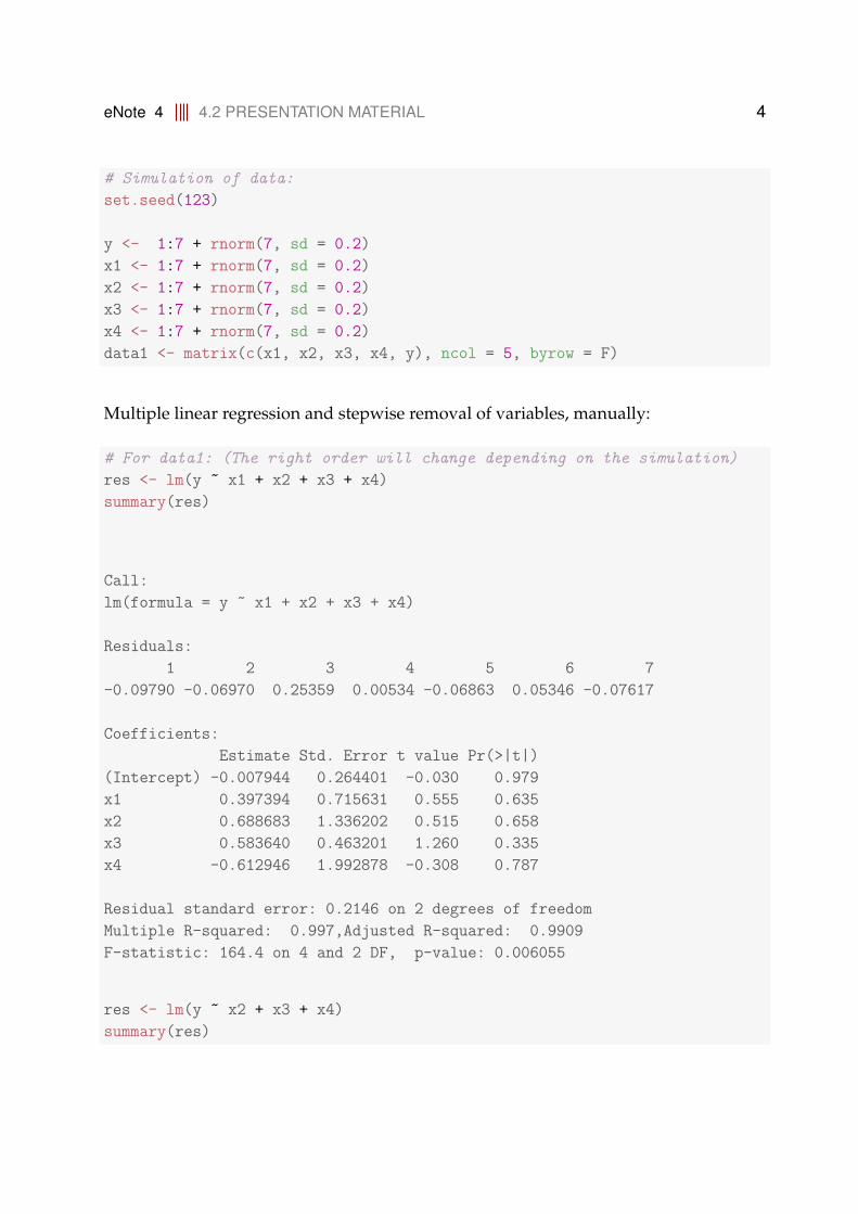
# Simulation of data:
set.seed(123)
y <- 1:7 + rnorm(7, sd = 0.2)
x1 <- 1:7 + rnorm(7, sd = 0.2)
x2 <- 1:7 + rnorm(7, sd = 0.2)
x3 <- 1:7 + rnorm(7, sd = 0.2)
x4 <- 1:7 + rnorm(7, sd = 0.2)
data1 <- matrix(c(x1, x2, x3, x4, y), ncol = 5, byrow = F)
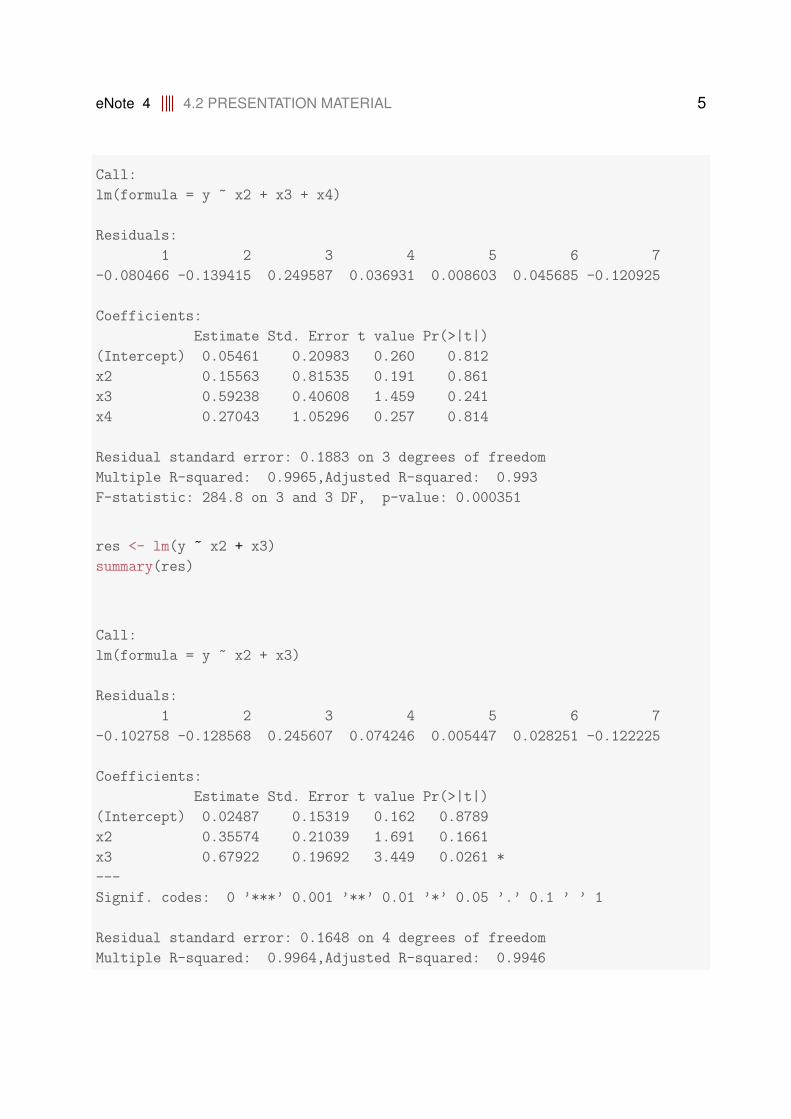
Multiple linear regression and stepwise removal of variables, manually:
# For data1: (The right order will change depending on the simulation)
res <- lm(y ~ x1 + x2 + x3 + x4)
summary(res)
Call:
lm(formula = y ~ x1 + x2 + x3 + x4)
Residuals:
1 2 3 4 5 6 7
-0.09790 -0.06970 0.25359 0.00534 -0.06863 0.05346 -0.07617
Coefficients:
Estimate Std. Error t value Pr(>|t|)
(Intercept) -0.007944 0.264401 -0.030 0.979
x1 0.397394 0.715631 0.555 0.635
x2 0.688683 1.336202 0.515 0.658
x3 0.583640 0.463201 1.260 0.335
x4 -0.612946 1.992878 -0.308 0.787
Residual standard error: 0.2146 on 2 degrees of freedom
Multiple R-squared: 0.997,Adjusted R-squared: 0.9909
F-statistic: 164.4 on 4 and 2 DF, p-value: 0.006055
res <- lm(y ~ x2 + x3 + x4)
summary(res)
eNote 4 4.2 PRESENTATION MATERIAL 5
Call:
lm(formula = y ~ x2 + x3 + x4)
Residuals:
1 2 3 4 5 6 7
-0.080466 -0.139415 0.249587 0.036931 0.008603 0.045685 -0.120925
Coefficients:
Estimate Std. Error t value Pr(>|t|)
(Intercept) 0.05461 0.20983 0.260 0.812
x2 0.15563 0.81535 0.191 0.861
x3 0.59238 0.40608 1.459 0.241
x4 0.27043 1.05296 0.257 0.814
Residual standard error: 0.1883 on 3 degrees of freedom
Multiple R-squared: 0.9965,Adjusted R-squared: 0.993
F-statistic: 284.8 on 3 and 3 DF, p-value: 0.000351
res <- lm(y ~ x2 + x3)
summary(res)
Call:
lm(formula = y ~ x2 + x3)
Residuals:
1 2 3 4 5 6 7
-0.102758 -0.128568 0.245607 0.074246 0.005447 0.028251 -0.122225
Coefficients:
Estimate Std. Error t value Pr(>|t|)
(Intercept) 0.02487 0.15319 0.162 0.8789
x2 0.35574 0.21039 1.691 0.1661
x3 0.67922 0.19692 3.449 0.0261 *
---
Signif. codes: 0 ’***’ 0.001 ’**’ 0.01 ’*’ 0.05 ’.’ 0.1 ’ ’ 1
Residual standard error: 0.1648 on 4 degrees of freedom
Multiple R-squared: 0.9964,Adjusted R-squared: 0.9946
eNote 4 4.2 PRESENTATION MATERIAL 6
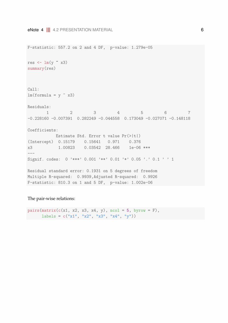
F-statistic: 557.2 on 2 and 4 DF, p-value: 1.279e-05
res <- lm(y ~ x3)
summary(res)
Call:
lm(formula = y ~ x3)
Residuals:
1 2 3 4 5 6 7
-0.228160 -0.007391 0.282249 -0.044558 0.173049 -0.027071 -0.148118
Coefficients:
Estimate Std. Error t value Pr(>|t|)
(Intercept) 0.15179 0.15641 0.971 0.376
x3 1.00823 0.03542 28.466 1e-06 ***
---
Signif. codes: 0 ’***’ 0.001 ’**’ 0.01 ’*’ 0.05 ’.’ 0.1 ’ ’ 1
Residual standard error: 0.1931 on 5 degrees of freedom
Multiple R-squared: 0.9939,Adjusted R-squared: 0.9926
F-statistic: 810.3 on 1 and 5 DF, p-value: 1.002e-06
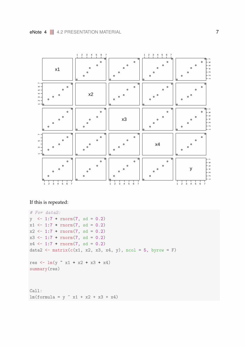
The pair-wise relations:
pairs(matrix(c(x1, x2, x3, x4, y), ncol = 5, byrow = F),
labels = c("x1", "x2", "x3", "x4", "y"))
eNote 4 4.2 PRESENTATION MATERIAL 7
x1
1 2 3 4 5 6 7
●
●
●
●
●
●
●
●
●
●
●
●
●
●
1 2 3 4 5 6 7
●
●
●
●
●
●
●
12
34
56
7
●
●
●
●
●
●
●
12
34
56
7
●
●
●
●
●
●
●
x2
●
●
●
●
●
●
●
●
●
●
●
●
●
●
●
●
●
●
●
●
●
●
●
●
●
●
●
●
●
●
●
●
●
●
●
x3
●
●
●
●
●
●
●
12
34
56
7
●
●
●
●
●
●
●
13
57
●
●
●
●
●
●
●
●
●
●
●
●
●
●
●
●
●
●
●
●
●
x4
●
●
●
●
●
●
●
1 2 3 4 5 6 7
●
●
●
●
●
●
●
●
●
●
●
●
●
●
1 2 3 4 5 6 7
●
●
●
●
●
●
●
●
●
●
●
●
●
●
1 2 3 4 5 6 7
12
34
56
7
y
If this is repeated:
# For data2:
y <- 1:7 + rnorm(7, sd = 0.2)
x1 <- 1:7 + rnorm(7, sd = 0.2)
x2 <- 1:7 + rnorm(7, sd = 0.2)
x3 <- 1:7 + rnorm(7, sd = 0.2)
x4 <- 1:7 + rnorm(7, sd = 0.2)
data2 <- matrix(c(x1, x2, x3, x4, y), ncol = 5, byrow = F)
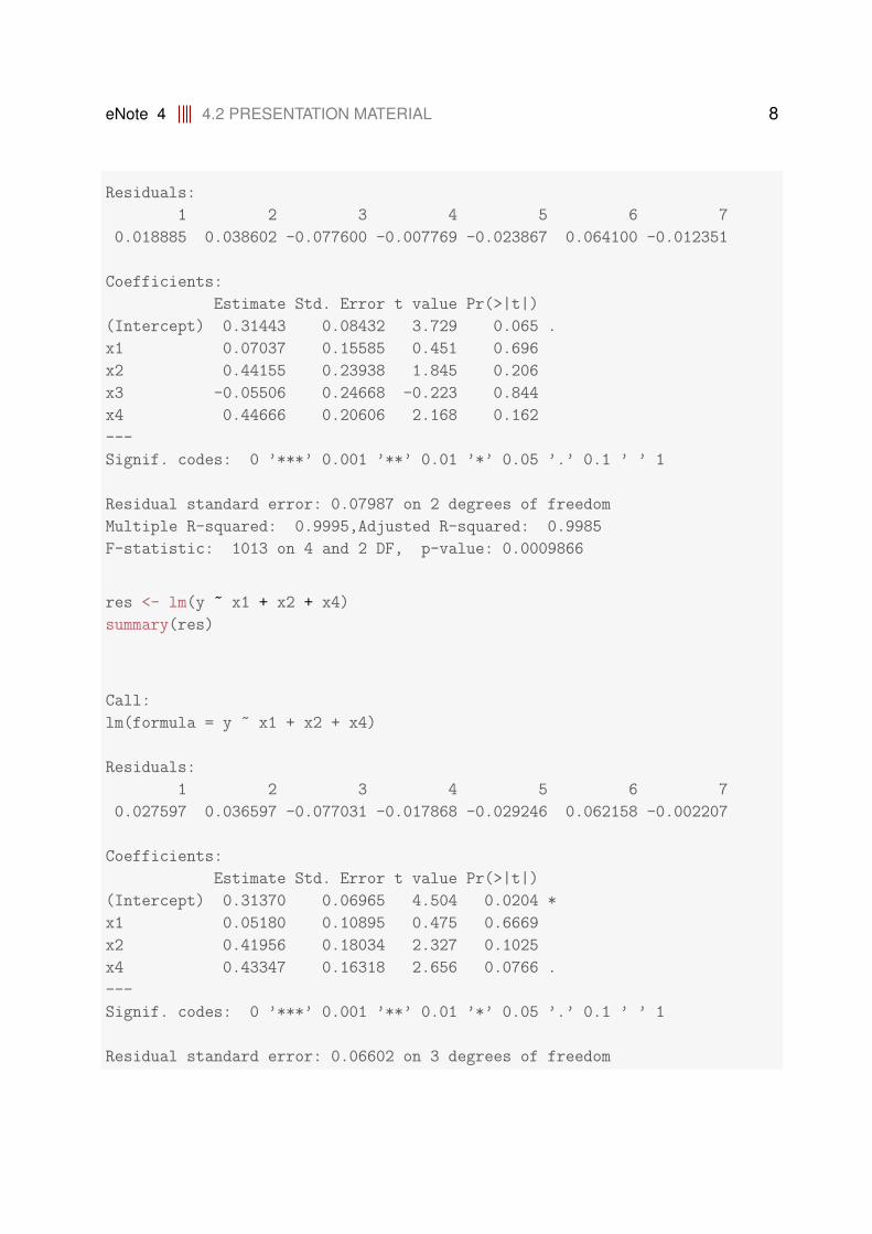
res <- lm(y ~ x1 + x2 + x3 + x4)
summary(res)
Call:
lm(formula = y ~ x1 + x2 + x3 + x4)
eNote 4 4.2 PRESENTATION MATERIAL 8
Residuals:
1 2 3 4 5 6 7
0.018885 0.038602 -0.077600 -0.007769 -0.023867 0.064100 -0.012351
Coefficients:
Estimate Std. Error t value Pr(>|t|)
(Intercept) 0.31443 0.08432 3.729 0.065 .
x1 0.07037 0.15585 0.451 0.696
x2 0.44155 0.23938 1.845 0.206
x3 -0.05506 0.24668 -0.223 0.844
x4 0.44666 0.20606 2.168 0.162
---
Signif. codes: 0 ’***’ 0.001 ’**’ 0.01 ’*’ 0.05 ’.’ 0.1 ’ ’ 1
Residual standard error: 0.07987 on 2 degrees of freedom
Multiple R-squared: 0.9995,Adjusted R-squared: 0.9985
F-statistic: 1013 on 4 and 2 DF, p-value: 0.0009866
res <- lm(y ~ x1 + x2 + x4)
summary(res)
Call:
lm(formula = y ~ x1 + x2 + x4)
Residuals:
1 2 3 4 5 6 7
0.027597 0.036597 -0.077031 -0.017868 -0.029246 0.062158 -0.002207
Coefficients:
Estimate Std. Error t value Pr(>|t|)
(Intercept) 0.31370 0.06965 4.504 0.0204 *
x1 0.05180 0.10895 0.475 0.6669
x2 0.41956 0.18034 2.327 0.1025
x4 0.43347 0.16318 2.656 0.0766 .
---
Signif. codes: 0 ’***’ 0.001 ’**’ 0.01 ’*’ 0.05 ’.’ 0.1 ’ ’ 1
Residual standard error: 0.06602 on 3 degrees of freedom
eNote 4 4.2 PRESENTATION MATERIAL 9
Multiple R-squared: 0.9995,Adjusted R-squared: 0.999
F-statistic: 1976 on 3 and 3 DF, p-value: 1.93e-05
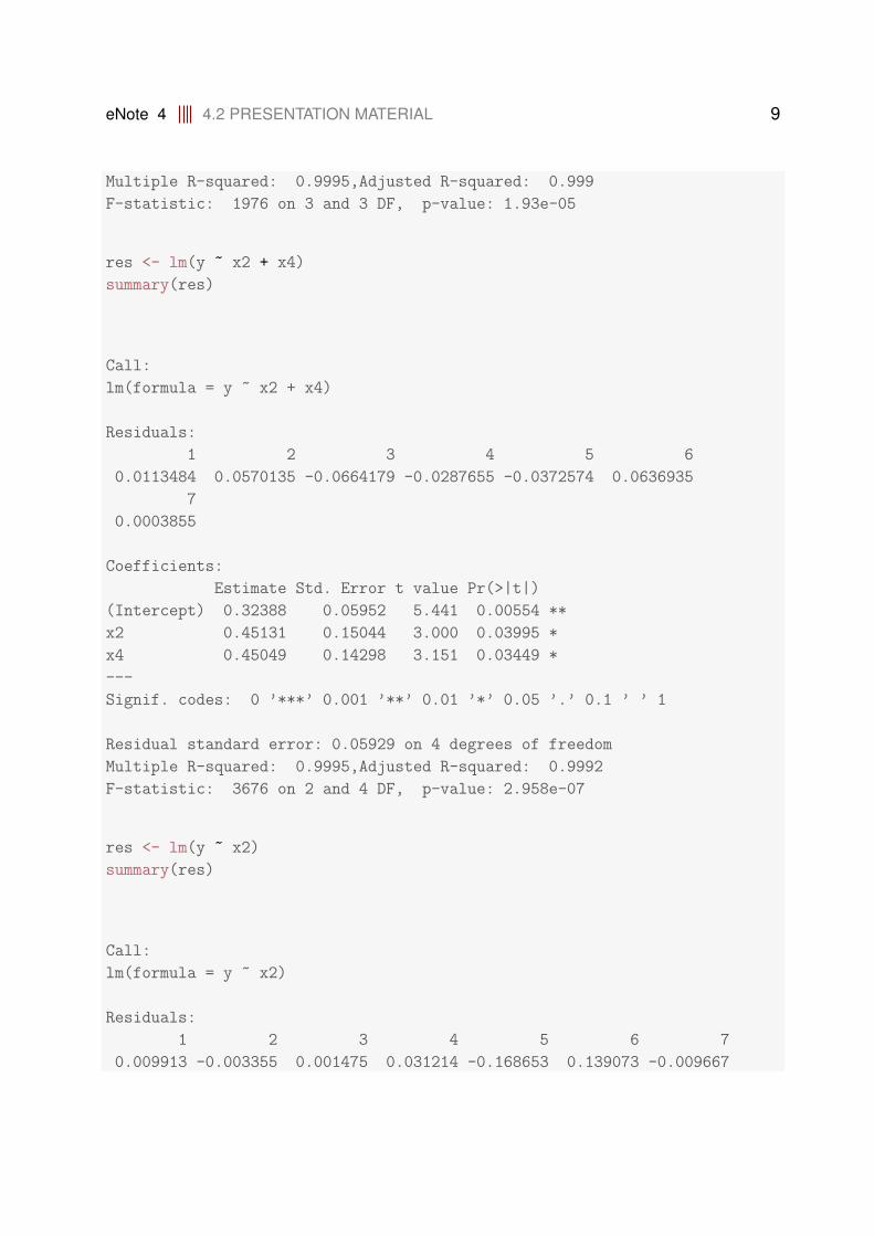
res <- lm(y ~ x2 + x4)
summary(res)
Call:
lm(formula = y ~ x2 + x4)
Residuals:
1 2 3 4 5 6
0.0113484 0.0570135 -0.0664179 -0.0287655 -0.0372574 0.0636935
7
0.0003855
Coefficients:
Estimate Std. Error t value Pr(>|t|)
(Intercept) 0.32388 0.05952 5.441 0.00554 **
x2 0.45131 0.15044 3.000 0.03995 *
x4 0.45049 0.14298 3.151 0.03449 *
---
Signif. codes: 0 ’***’ 0.001 ’**’ 0.01 ’*’ 0.05 ’.’ 0.1 ’ ’ 1
Residual standard error: 0.05929 on 4 degrees of freedom
Multiple R-squared: 0.9995,Adjusted R-squared: 0.9992
F-statistic: 3676 on 2 and 4 DF, p-value: 2.958e-07
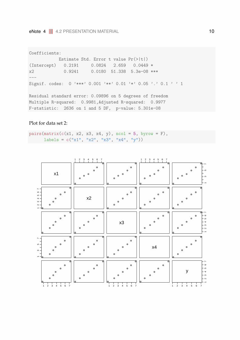
res <- lm(y ~ x2)
summary(res)
Call:
lm(formula = y ~ x2)
Residuals:
1 2 3 4 5 6 7
0.009913 -0.003355 0.001475 0.031214 -0.168653 0.139073 -0.009667
eNote 4 4.2 PRESENTATION MATERIAL 10
Coefficients:
Estimate Std. Error t value Pr(>|t|)
(Intercept) 0.2191 0.0824 2.659 0.0449 *
x2 0.9241 0.0180 51.338 5.3e-08 ***
---
Signif. codes: 0 ’***’ 0.001 ’**’ 0.01 ’*’ 0.05 ’.’ 0.1 ’ ’ 1
Residual standard error: 0.09896 on 5 degrees of freedom
Multiple R-squared: 0.9981,Adjusted R-squared: 0.9977
F-statistic: 2636 on 1 and 5 DF, p-value: 5.301e-08
Plot for data set 2:
pairs(matrix(c(x1, x2, x3, x4, y), ncol = 5, byrow = F),
labels = c("x1", "x2", "x3", "x4", "y"))
x1
1 2 3 4 5 6 7
●
●
●●
●
●
●
●
●
●●
●
●
●
1 2 3 4 5 6 7
●
●
●●
●
●
●
13
57
●
●
●●
●
●
●
12
34
56
7
●
●
●
●
●
●
●
x2
●
●
●
●
●
●
●
●
●
●
●
●
●
●
●
●
●
●
●
●
●
●
●
●
●
●
●
●
●
●
●
●
●
●
●
x3
●
●
●
●
●
●
●
12
34
56
7
●
●
●
●
●
●
●
13
57
●
●
●
●
●
●
●
●
●
●
●
●
●
●
●
●
●
●
●
●
●
x4
●
●
●
●
●
●
●
1 2 3 4 5 6 7
●
●
●
●
●
●
●
●
●
●
●
●
●
●
1 2 3 4 5 6 7
●
●
●
●
●
●
●
●
●
●
●
●
●
●
1 2 3 4 5 6 7
12
34
56
7
y
eNote 4 4.2 PRESENTATION MATERIAL 11
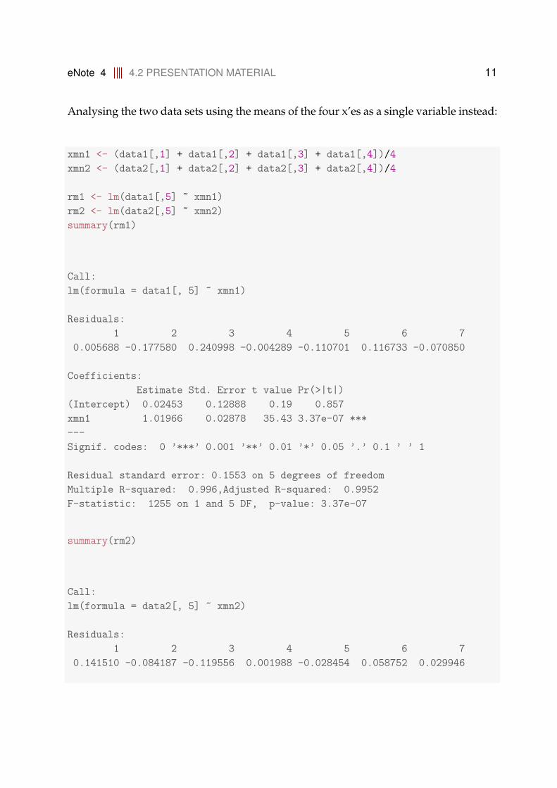
Analysing the two data sets using the means of the four x’es as a single variable instead:
xmn1 <- (data1[,1] + data1[,2] + data1[,3] + data1[,4])/4
xmn2 <- (data2[,1] + data2[,2] + data2[,3] + data2[,4])/4
rm1 <- lm(data1[,5] ~ xmn1)
rm2 <- lm(data2[,5] ~ xmn2)
summary(rm1)
Call:
lm(formula = data1[, 5] ~ xmn1)
Residuals:
1 2 3 4 5 6 7
0.005688 -0.177580 0.240998 -0.004289 -0.110701 0.116733 -0.070850
Coefficients:
Estimate Std. Error t value Pr(>|t|)
(Intercept) 0.02453 0.12888 0.19 0.857
xmn1 1.01966 0.02878 35.43 3.37e-07 ***
---
Signif. codes: 0 ’***’ 0.001 ’**’ 0.01 ’*’ 0.05 ’.’ 0.1 ’ ’ 1
Residual standard error: 0.1553 on 5 degrees of freedom
Multiple R-squared: 0.996,Adjusted R-squared: 0.9952
F-statistic: 1255 on 1 and 5 DF, p-value: 3.37e-07
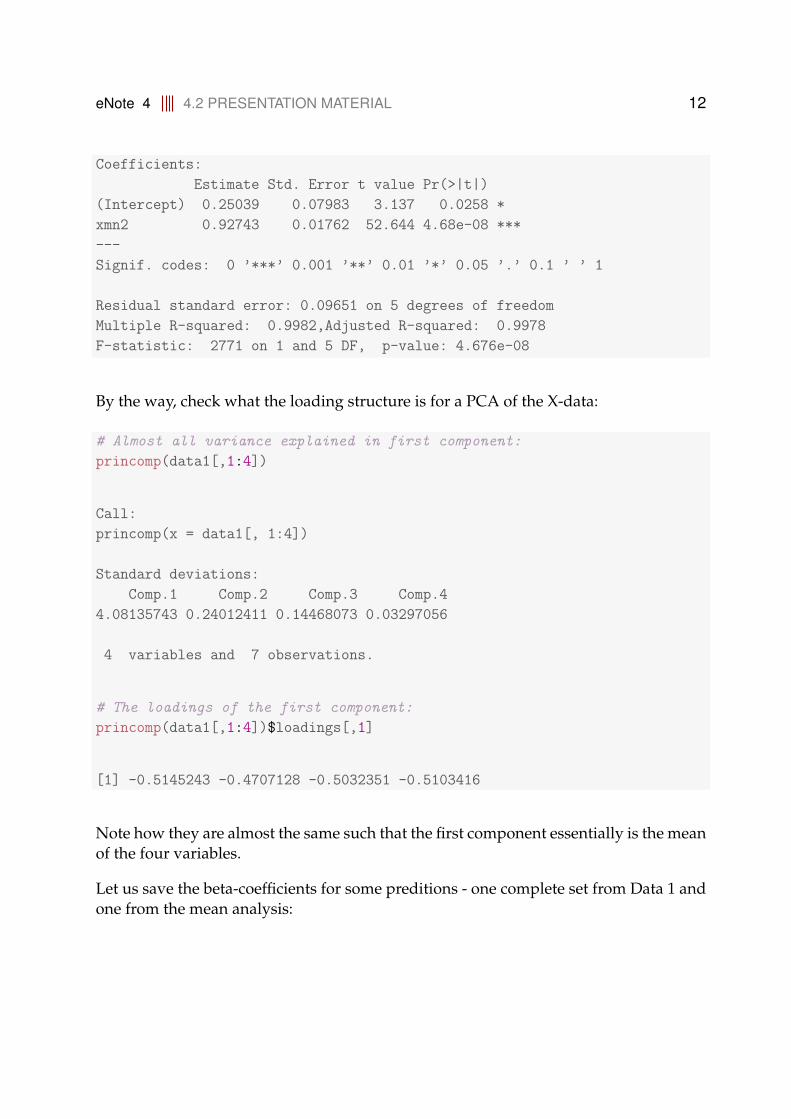
summary(rm2)
Call:
lm(formula = data2[, 5] ~ xmn2)
Residuals:
1 2 3 4 5 6 7
0.141510 -0.084187 -0.119556 0.001988 -0.028454 0.058752 0.029946
eNote 4 4.2 PRESENTATION MATERIAL 12
Coefficients:
Estimate Std. Error t value Pr(>|t|)
(Intercept) 0.25039 0.07983 3.137 0.0258 *
xmn2 0.92743 0.01762 52.644 4.68e-08 ***
---
Signif. codes: 0 ’***’ 0.001 ’**’ 0.01 ’*’ 0.05 ’.’ 0.1 ’ ’ 1
Residual standard error: 0.09651 on 5 degrees of freedom
Multiple R-squared: 0.9982,Adjusted R-squared: 0.9978
F-statistic: 2771 on 1 and 5 DF, p-value: 4.676e-08
By the way, check what the loading structure is for a PCA of the X-data:
# Almost all variance explained in first component:
princomp(data1[,1:4])
Call:
princomp(x = data1[, 1:4])
Standard deviations:
Comp.1 Comp.2 Comp.3 Comp.4
4.08135743 0.24012411 0.14468073 0.03297056
4 variables and 7 observations.
# The loadings of the first component:
princomp(data1[,1:4])$loadings[,1]
[1] -0.5145243 -0.4707128 -0.5032351 -0.5103416
Note how they are almost the same such that the first component essentially is the meanof the four variables.
Let us save the beta-coefficients for some preditions - one complete set from Data 1 andone from the mean analysis:
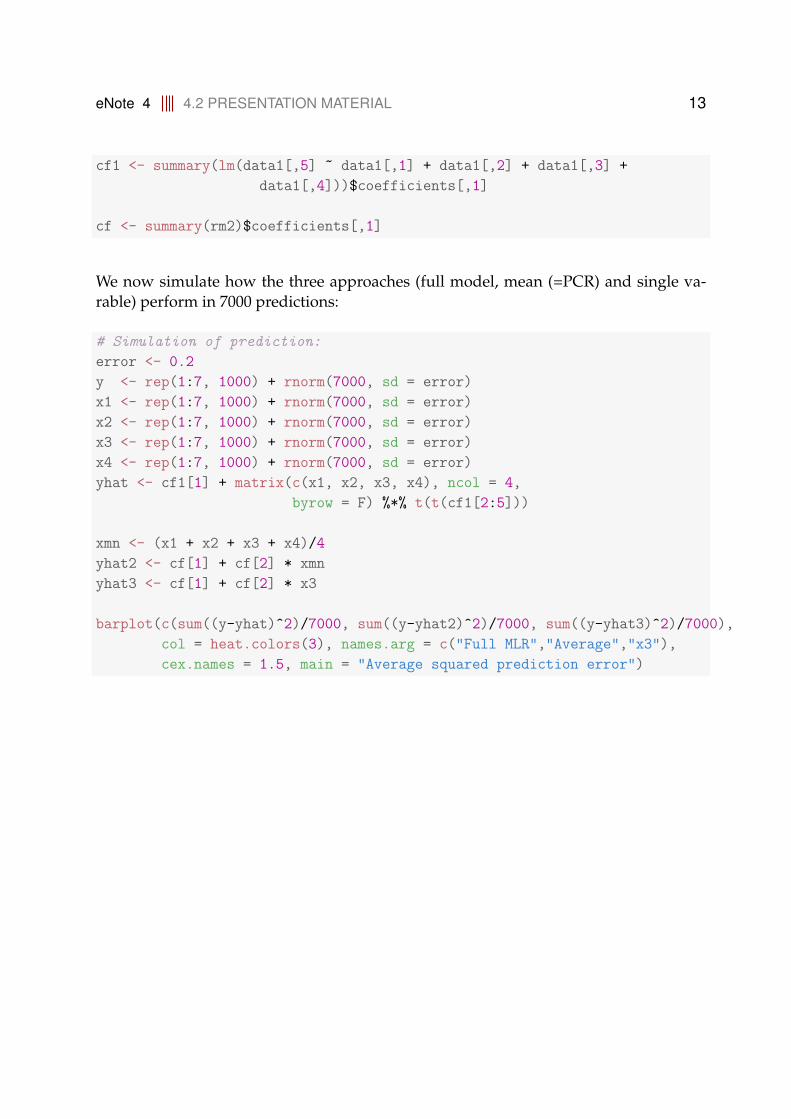
eNote 4 4.2 PRESENTATION MATERIAL 13
cf1 <- summary(lm(data1[,5] ~ data1[,1] + data1[,2] + data1[,3] +
data1[,4]))$coefficients[,1]
cf <- summary(rm2)$coefficients[,1]
We now simulate how the three approaches (full model, mean (=PCR) and single va-rable) perform in 7000 predictions:
# Simulation of prediction:
error <- 0.2
y <- rep(1:7, 1000) + rnorm(7000, sd = error)
x1 <- rep(1:7, 1000) + rnorm(7000, sd = error)
x2 <- rep(1:7, 1000) + rnorm(7000, sd = error)
x3 <- rep(1:7, 1000) + rnorm(7000, sd = error)
x4 <- rep(1:7, 1000) + rnorm(7000, sd = error)
yhat <- cf1[1] + matrix(c(x1, x2, x3, x4), ncol = 4,
byrow = F) %*% t(t(cf1[2:5]))
xmn <- (x1 + x2 + x3 + x4)/4
yhat2 <- cf[1] + cf[2] * xmn
yhat3 <- cf[1] + cf[2] * x3
barplot(c(sum((y-yhat)^2)/7000, sum((y-yhat2)^2)/7000, sum((y-yhat3)^2)/7000),
col = heat.colors(3), names.arg = c("Full MLR","Average","x3"),
cex.names = 1.5, main = "Average squared prediction error")
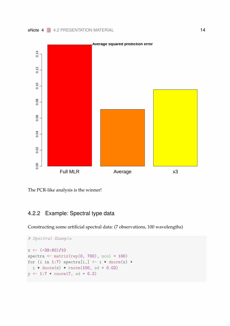
eNote 4 4.2 PRESENTATION MATERIAL 14
Full MLR Average x3
Average squared prediction error
0.00
0.02
0.04
0.06
0.08
0.10
0.12
0.14
The PCR-like analysis is the winner!
4.2.2 Example: Spectral type data
Constructing some artificial spectral data: (7 observations, 100 wavelengths)
# Spectral Example
x <- (-39:60)/10
spectra <- matrix(rep(0, 700), ncol = 100)
for (i in 1:7) spectra[i,] <- i * dnorm(x) +
i * dnorm(x) * rnorm(100, sd = 0.02)
y <- 1:7 + rnorm(7, sd = 0.2)
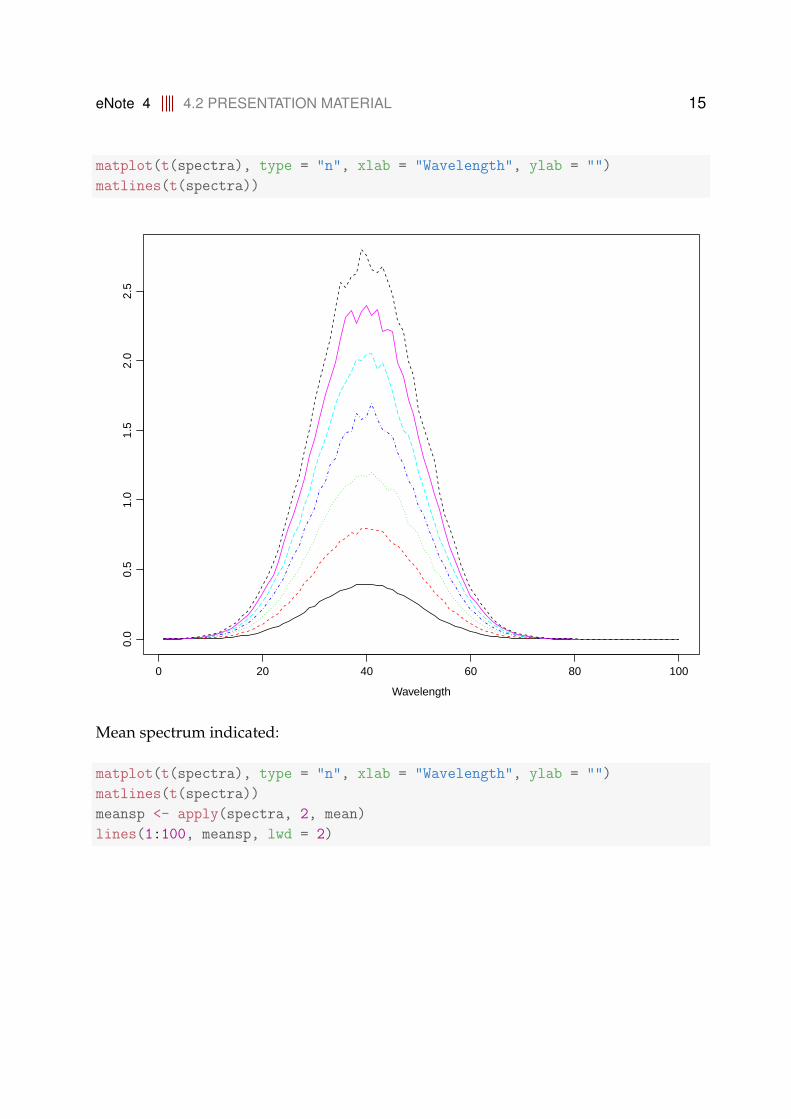
eNote 4 4.2 PRESENTATION MATERIAL 15
matplot(t(spectra), type = "n", xlab = "Wavelength", ylab = "")
matlines(t(spectra))
0 20 40 60 80 100
0.0
0.5
1.0
1.5
2.0
2.5
Wavelength
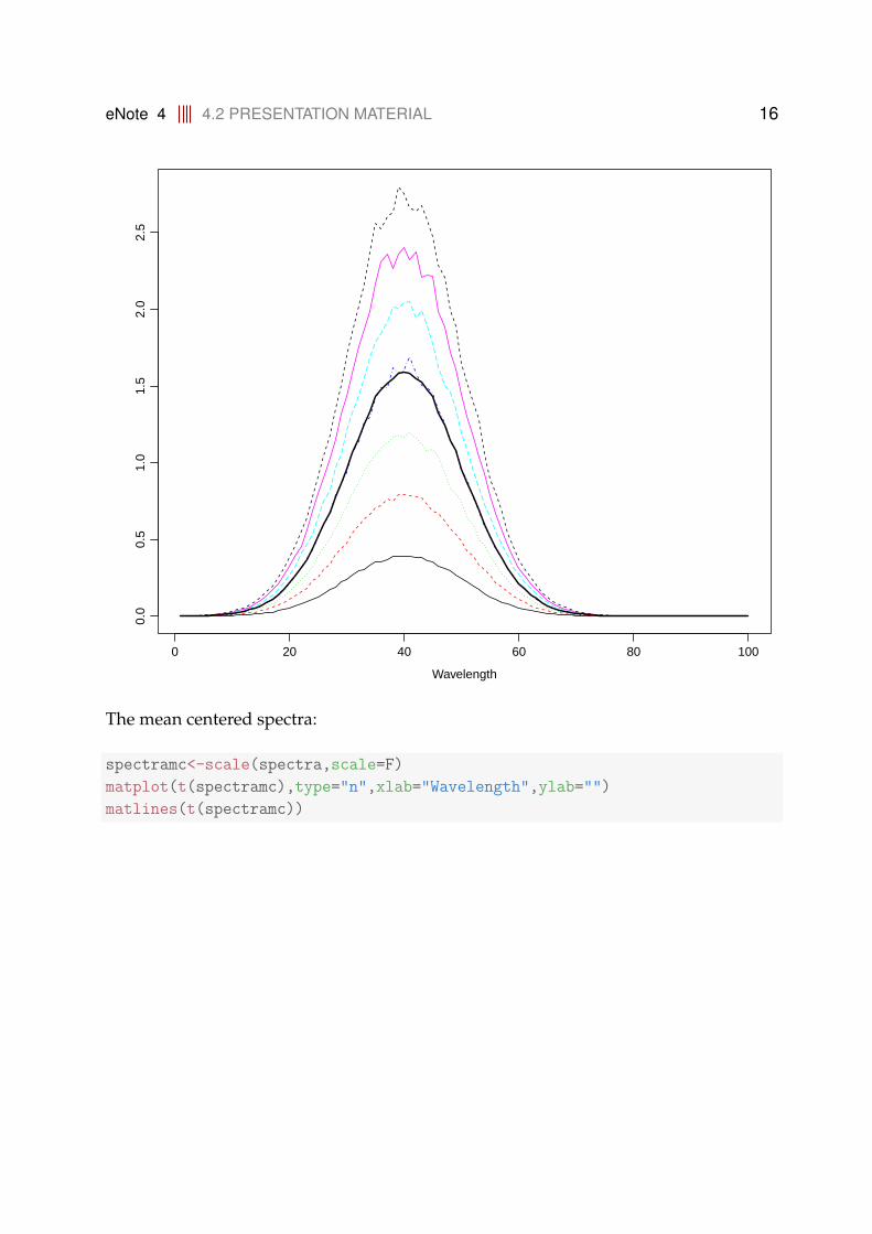
Mean spectrum indicated:
matplot(t(spectra), type = "n", xlab = "Wavelength", ylab = "")
matlines(t(spectra))
meansp <- apply(spectra, 2, mean)
lines(1:100, meansp, lwd = 2)
eNote 4 4.2 PRESENTATION MATERIAL 16
0 20 40 60 80 100
0.0
0.5
1.0
1.5
2.0
2.5
Wavelength
The mean centered spectra:
spectramc<-scale(spectra,scale=F)
matplot(t(spectramc),type="n",xlab="Wavelength",ylab="")
matlines(t(spectramc))
eNote 4 4.2 PRESENTATION MATERIAL 17
0 20 40 60 80 100
−1.
0−
0.5
0.0
0.5
1.0
Wavelength
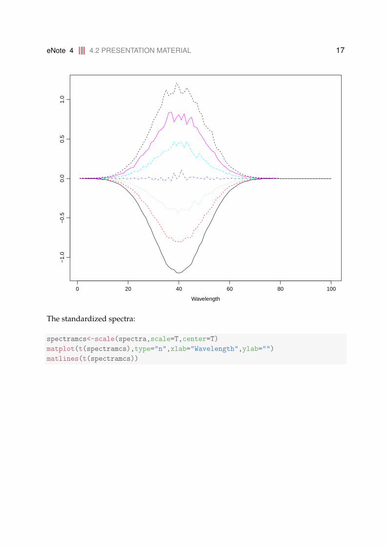
The standardized spectra:
spectramcs<-scale(spectra,scale=T,center=T)
matplot(t(spectramcs),type="n",xlab="Wavelength",ylab="")
matlines(t(spectramcs))
eNote 4 4.2 PRESENTATION MATERIAL 18
0 20 40 60 80 100
−1.
5−
1.0
−0.
50.
00.
51.
01.
5
Wavelength
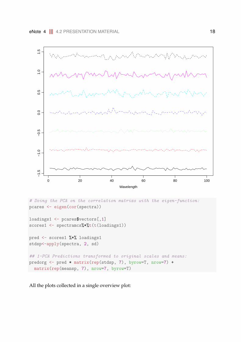
# Doing the PCA on the correlation matrixs with the eigen-function:
pcares <- eigen(cor(spectra))
loadings1 <- pcares$vectors[,1]
scores1 <- spectramcs%*%t(t(loadings1))
pred <- scores1 %*% loadings1
stdsp<-apply(spectra, 2, sd)
## 1-PCA Predictions transformed to original scales and means:
predorg <- pred * matrix(rep(stdsp, 7), byrow=T, nrow=7) +
matrix(rep(meansp, 7), nrow=7, byrow=T)
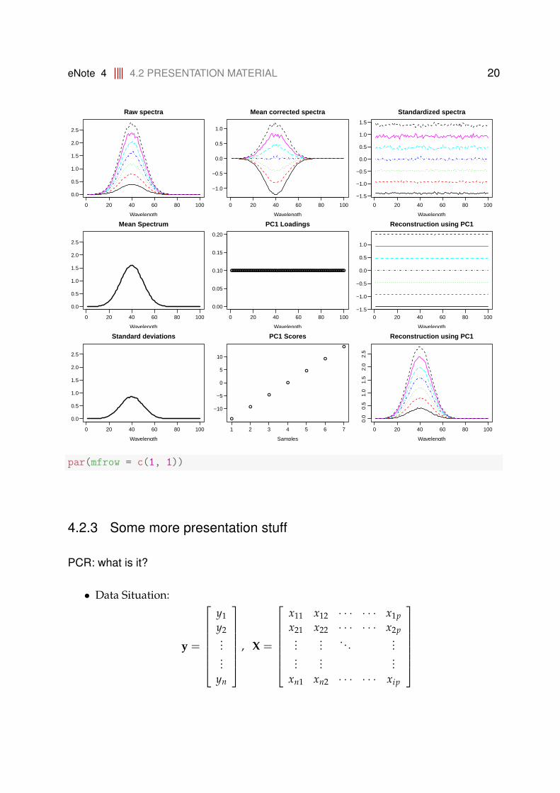
All the plots collected in a single overview plot:
eNote 4 4.2 PRESENTATION MATERIAL 19
par(mfrow = c(3, 3), mar = 0.6 * c(5, 4, 4, 2))
matplot(t(spectra), type = "n", xlab = "Wavelength",
ylab = "", main = "Raw spectra", las = 1)
matlines(t(spectra))
matplot(t(spectramc), type = "n", xlab = "Wavelength",
ylab = "", main = "Mean corrected spectra", las = 1)
matlines(t(spectramc))
matplot(t(spectramcs), type = "n", xlab = "Wavelength",
ylab = "", main = "Standardized spectra", las = 1)
matlines(t(spectramcs))
matplot(t(spectra), type = "n", xlab = "Wavelength",
ylab = "", main = "Mean Spectrum", las = 1)
lines(1:100, meansp, lwd = 2)
plot(1:100, -loadings1, ylim = c(0, 0.2), xlab = "Wavelength",
ylab = "", main = "PC1 Loadings", las = 1)
matplot(t(pred), type = "n", xlab = "Wavelength",
ylab = "", main = "Reconstruction using PC1", las = 1)
matlines(t(pred))
matplot(t(spectra), type = "n", xlab = "Wavelength",
ylab = "", main = "Standard deviations", las = 1)
lines(1:100, stdsp, lwd = 2)
plot(1:7, scores1[7:1], main = "PC1 Scores", xlab = "Samples",
ylab = "", las = 1)
matplot(t(predorg), type = "n", xlab = "Wavelength",
ylab = "", main = "Reconstruction using PC1")
matlines(t(predorg))
eNote 4 4.2 PRESENTATION MATERIAL 20
0 20 40 60 80 100
0.0
0.5
1.0
1.5
2.0
2.5
Raw spectra
Wavelength
0 20 40 60 80 100
−1.0
−0.5
0.0
0.5
1.0
Mean corrected spectra
Wavelength
0 20 40 60 80 100
−1.5
−1.0
−0.5
0.0
0.5
1.0
1.5
Standardized spectra
Wavelength
0 20 40 60 80 100
0.0
0.5
1.0
1.5
2.0
2.5
Mean Spectrum
Wavelength
●●●●●●●●●●●●●●●●●●●●●●●●●●●●●●●●●●●●●●●●●●●●●●●●●●●●●●●●●●●●●●●●●●●●●●●●●●●●●●●●●●●●●●●●●●●●●●●●●●●●
0 20 40 60 80 100
0.00
0.05
0.10
0.15
0.20
PC1 Loadings
Wavelength
0 20 40 60 80 100−1.5
−1.0
−0.5
0.0
0.5
1.0
Reconstruction using PC1
Wavelength
0 20 40 60 80 100
0.0
0.5
1.0
1.5
2.0
2.5
Standard deviations
Wavelength
●
●
●
●
●
●
●
1 2 3 4 5 6 7
−10
−5
0
5
10
PC1 Scores
Samples
0 20 40 60 80 100
0.0
0.5
1.0
1.5
2.0
2.5
Reconstruction using PC1
Wavelength
par(mfrow = c(1, 1))
4.2.3 Some more presentation stuff
PCR: what is it?
• Data Situation:
y =
y1y2......
yn
, X =
x11 x12 · · · · · · x1px21 x22 · · · · · · x2p
...... . . . ...
......
...xn1 xn2 · · · · · · xip

eNote 4 4.2 PRESENTATION MATERIAL 21
• Do MLR with A principal components t1, . . . , tA instead of all (or some) of the x’s.
• How many components: Determine by Cross-validation!
How to do it?
1. Explore data
2. Do modelling (choose number of components, consider variable selection)
3. Validate (residuals, outliers, influence etc)
4. Iterate e.g. on 2. and 3.
5. Interpret, conclude, report.
6. If relevant: predict future values.
Cross Validation ("Full")
• Leave out one of the observations
• Fit a model on the remaining(reduced) data
• Predict the left out observation by the model: yi,val
• Do this in turn for ALL observations AND calculate the overall performance ofthe model:
RMSEP =
√n
∑i(yi − yi,val)2/n
(Root Mean Squared Error of Prediction)
Cross Validation ("Full")
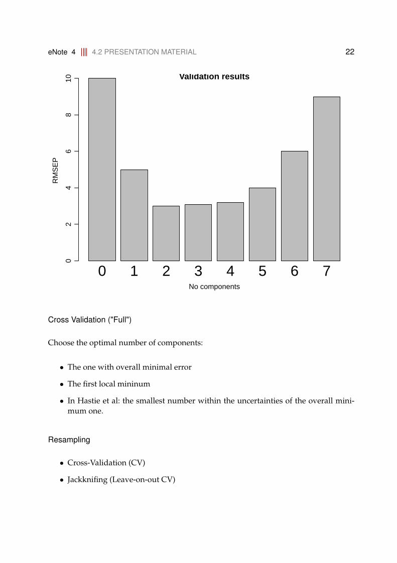
Finally: Do the cross-validation for ALL choices of number of components (0, 1, 2, . . . , . . .)AND plot the performances, e.g.: (constructed plot)
barplot(c(10, 5, 3, 3.1, 3.2, 4, 6, 9), names.arg = 0:7,
xlab = "No components", ylab = "RMSEP", cex.names = 2,
main = "Validation results")
eNote 4 4.2 PRESENTATION MATERIAL 22
0 1 2 3 4 5 6 7
Validation results
No components
RM
SE
P
02
46
810
Cross Validation ("Full")
Choose the optimal number of components:
• The one with overall minimal error
• The first local mininum
• In Hastie et al: the smallest number within the uncertainties of the overall mini-mum one.
Resampling
• Cross-Validation (CV)
• Jackknifing (Leave-on-out CV)
eNote 4 4.2 PRESENTATION MATERIAL 23
• Bootstrapping
• A good generic approach:
– Split the data into a TRAINING and a TEST set.
– Use Cross-validation on the TRAINING data
– Check the model performance on the TEST-set
– MAYBE: REPEAT all this many times (Repeated Double Cross Validation)
Cross Validation - principle
• Minimizes the expected prediction error:
Squared Prediction error = Bias2 + Variance
• Including ”many”PC-components: LOW bias, but HIGH variance
• Including ”few”PC-components: HIGH bias, but LOW variance
• Choose the best compromise!
• Note: Including ALL components = MLR (when n > p)
Validation - exist on different levels
1. Split in 3: Training(50%), Validation(25%) and Test(25%)
• Requires many observations - Rarely used
2. Split in 2: Calibration/training (67% ) and Test(33%) - us CV/bootstrap within thetraining
• more commonly used
3. No ”fixed split”, but repeated splits by CV/bootstrap, and then CV within eachtraining set (”Repeated double CV”)
4. No split, but using (one level of) CV/bootstrap.
5. Just fitting on all - and checking the error.

eNote 4 4.3 EXAMPLE: CAR DATA (AGAIN) 24
4.3 Example: Car Data (again)
# Example: using Car data:
data(mtcars)
mtcars$logmpg <- log(mtcars$mpg)
# Define the X-matrix as a matrix in the data frame:
mtcars$X <- as.matrix(mtcars[, 2:11])
# First of all we consider a random selection of 4 properties as a TEST set
mtcars$train <- TRUE
mtcars$train[sample(1:length(mtcars$train), 4)] <- FALSE
mtcars_TEST <- mtcars[mtcars$train == FALSE,]
mtcars_TRAIN <- mtcars[mtcars$train == TRUE,]
Now all the work is performed on the TRAIN data set.
Explore the data
We allready did this previously, so no more of that here
Next: Model the data
Run the PCR with maximal/large number of components using pls package:
# Run the PCR with maximal/large number of components using pls package:
library(pls)
mod <- pcr(logmpg ~ X , ncomp = 10, data = mtcars_TRAIN,
validation="LOO", scale = TRUE, jackknife = TRUE)
Initial set of plots:
# Initial set of plots:
par(mfrow = c(2, 2))
eNote 4 4.3 EXAMPLE: CAR DATA (AGAIN) 25
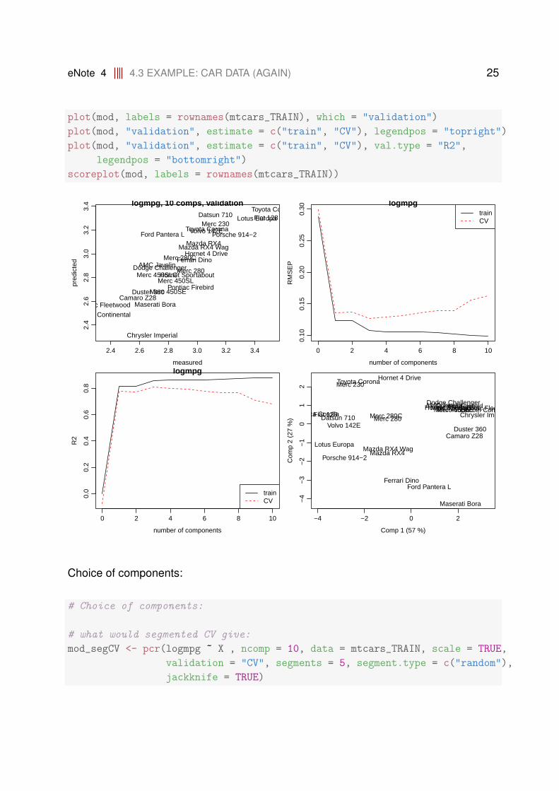
plot(mod, labels = rownames(mtcars_TRAIN), which = "validation")
plot(mod, "validation", estimate = c("train", "CV"), legendpos = "topright")
plot(mod, "validation", estimate = c("train", "CV"), val.type = "R2",
legendpos = "bottomright")
scoreplot(mod, labels = rownames(mtcars_TRAIN))
2.4 2.6 2.8 3.0 3.2 3.4
2.4
2.6
2.8
3.0
3.2
3.4 logmpg, 10 comps, validation
measured
pred
icte
d
Mazda RX4Mazda RX4 Wag
Datsun 710
Hornet 4 Drive
Hornet Sportabout
Duster 360
Merc 230
Merc 280
Merc 280C
Merc 450SE
Merc 450SLMerc 450SLC
Cadillac Fleetwood
Lincoln Continental
Chrysler Imperial
Fiat 128Toyota Corolla
Toyota Corona
Dodge ChallengerAMC Javelin
Camaro Z28
Pontiac Firebird
Porsche 914−2
Lotus Europa
Ford Pantera L
Ferrari Dino
Maserati Bora
Volvo 142E
0 2 4 6 8 10
0.10
0.15
0.20
0.25
0.30
logmpg
number of components
RM
SE
P
trainCV
0 2 4 6 8 10
0.0
0.2
0.4
0.6
0.8
logmpg
number of components
R2
trainCV
−4 −2 0 2
−4
−3
−2
−1
01
2
Comp 1 (57 %)
Com
p 2
(27
%)
Mazda RX4Mazda RX4 Wag
Datsun 710
Hornet 4 Drive
Hornet Sportabout
Duster 360
Merc 230
Merc 280Merc 280CMerc 450SEMerc 450SLMerc 450SLCCadillac FleetwoodLincoln Continental
Chrysler ImperialFiat 128Toyota Corolla
Toyota Corona
Dodge ChallengerAMC Javelin
Camaro Z28
Pontiac Firebird
Porsche 914−2
Lotus Europa
Ford Pantera LFerrari Dino
Maserati Bora
Volvo 142E
Choice of components:
# Choice of components:
# what would segmented CV give:
mod_segCV <- pcr(logmpg ~ X , ncomp = 10, data = mtcars_TRAIN, scale = TRUE,
validation = "CV", segments = 5, segment.type = c("random"),
jackknife = TRUE)
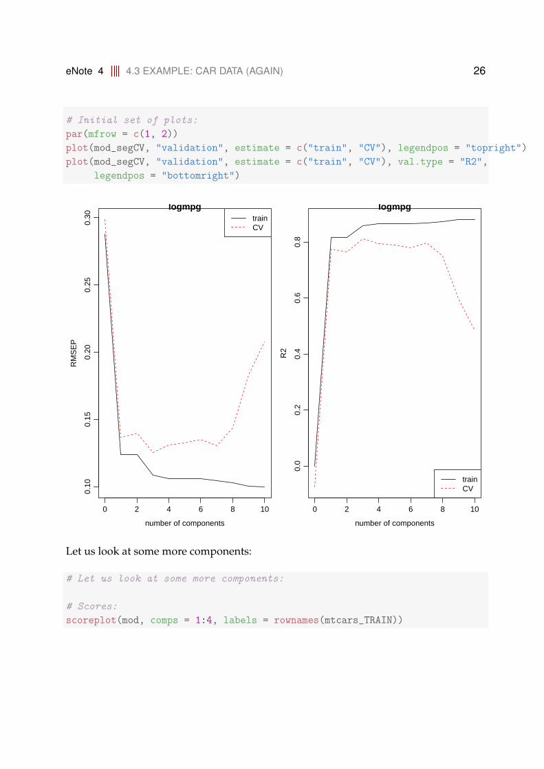
eNote 4 4.3 EXAMPLE: CAR DATA (AGAIN) 26
# Initial set of plots:
par(mfrow = c(1, 2))
plot(mod_segCV, "validation", estimate = c("train", "CV"), legendpos = "topright")
plot(mod_segCV, "validation", estimate = c("train", "CV"), val.type = "R2",
legendpos = "bottomright")
0 2 4 6 8 10
0.10
0.15
0.20
0.25
0.30
logmpg
number of components
RM
SE
P
trainCV
0 2 4 6 8 10
0.0
0.2
0.4
0.6
0.8
logmpg
number of components
R2
trainCV
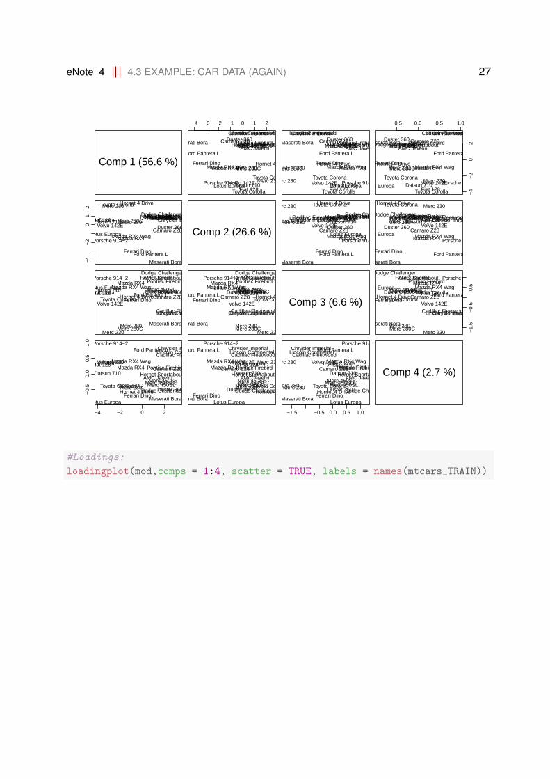
Let us look at some more components:
# Let us look at some more components:
# Scores:
scoreplot(mod, comps = 1:4, labels = rownames(mtcars_TRAIN))
eNote 4 4.3 EXAMPLE: CAR DATA (AGAIN) 27
Comp 1 (56.6 %)
−4 −3 −2 −1 0 1 2
Mazda RX4Mazda RX4 Wag
Datsun 710
Hornet 4 Drive
Hornet SportaboutDuster 360
Merc 230
Merc 280Merc 280C
Merc 450SEMerc 450SLMerc 450SLC
Cadillac FleetwoodLincoln ContinentalChrysler Imperial
Fiat 128Toyota Corolla
Toyota Corona
Dodge ChallengerAMC Javelin
Camaro Z28Pontiac Firebird
Porsche 914−2Lotus Europa
Ford Pantera L
Ferrari Dino
Maserati Bora
Volvo 142E
−0.5 0.0 0.5 1.0
−4
−2
02
Mazda RX4Mazda RX4 Wag
Datsun 710
Hornet 4 Drive
Hornet SportaboutDuster 360
Merc 230
Merc 280Merc 280C
Merc 450SEMerc 450SLMerc 450SLC
Cadillac FleetwoodLincoln ContinentalChrysler Imperial
Fiat 128Toyota Corolla
Toyota Corona
Dodge ChallengerAMC Javelin
Camaro Z28Pontiac Firebird
Porsche 914−2Lotus Europa
Ford Pantera L
Ferrari Dino
Maserati Bora
Volvo 142E
−4
−2
01
2
Mazda RX4Mazda RX4 Wag
Datsun 710
Hornet 4 Drive
Hornet Sportabout
Duster 360
Merc 230
Merc 280Merc 280C Merc 450SEMerc 450SLMerc 450SLCCadillac FleetwoodLincoln ContinentalChrysler ImperialFiat 128Toyota Corolla
Toyota Corona
Dodge ChallengerAMC Javelin
Camaro Z28
Pontiac Firebird
Porsche 914−2Lotus Europa
Ford Pantera LFerrari Dino
Maserati Bora
Volvo 142E
Comp 2 (26.6 %)Mazda RX4Mazda RX4 Wag
Datsun 710
Hornet 4 Drive
Hornet Sportabout
Duster 360
Merc 230
Merc 280Merc 280C Merc 450SEMerc 450SLMerc 450SLCCadillac FleetwoodLincoln ContinentalChrysler ImperialFiat 128Toyota Corolla
Toyota Corona
Dodge ChallengerAMC Javelin
Camaro Z28
Pontiac Firebird
Porsche 914−2Lotus Europa
Ford Pantera LFerrari Dino
Maserati Bora
Volvo 142E
Mazda RX4Mazda RX4 Wag
Datsun 710
Hornet 4 Drive
Hornet Sportabout
Duster 360
Merc 230
Merc 280Merc 280CMerc 450SEMerc 450SLMerc 450SLCCadillac FleetwoodLincoln ContinentalChrysler ImperialFiat 128Toyota Corolla
Toyota Corona
Dodge ChallengerAMC Javelin
Camaro Z28
Pontiac Firebird
Porsche 914−2Lotus Europa
Ford Pantera LFerrari Dino
Maserati Bora
Volvo 142E
Mazda RX4Mazda RX4 WagDatsun 710
Hornet 4 Drive
Hornet Sportabout
Duster 360
Merc 230Merc 280Merc 280C
Merc 450SEMerc 450SLMerc 450SLC
Cadillac FleetwoodLincoln ContinentalChrysler Imperial
Fiat 128Toyota CorollaToyota Corona
Dodge ChallengerAMC Javelin
Camaro Z28
Pontiac FirebirdPorsche 914−2
Lotus EuropaFord Pantera L
Ferrari Dino
Maserati Bora
Volvo 142E
Mazda RX4Mazda RX4 WagDatsun 710
Hornet 4 Drive
Hornet Sportabout
Duster 360
Merc 230Merc 280Merc 280C
Merc 450SEMerc 450SLMerc 450SLC
Cadillac FleetwoodLincoln ContinentalChrysler Imperial
Fiat 128Toyota CorollaToyota Corona
Dodge ChallengerAMC Javelin
Camaro Z28
Pontiac FirebirdPorsche 914−2
Lotus EuropaFord Pantera L
Ferrari Dino
Maserati Bora
Volvo 142E Comp 3 (6.6 %)
−1.
5−
0.5
0.5Mazda RX4
Mazda RX4 WagDatsun 710Hornet 4 Drive
Hornet Sportabout
Duster 360
Merc 230Merc 280Merc 280C
Merc 450SEMerc 450SLMerc 450SLC
Cadillac FleetwoodLincoln ContinentalChrysler Imperial
Fiat 128Toyota CorollaToyota Corona
Dodge ChallengerAMC Javelin
Camaro Z28
Pontiac FirebirdPorsche 914−2
Lotus EuropaFord Pantera L
Ferrari Dino
Maserati Bora
Volvo 142E
−4 −2 0 2
−0.
50.
00.
51.
0
Mazda RX4Mazda RX4 Wag
Datsun 710
Hornet 4 Drive
Hornet Sportabout
Duster 360
Merc 230
Merc 280Merc 280CMerc 450SEMerc 450SLMerc 450SLC
Cadillac FleetwoodLincoln ContinentalChrysler Imperial
Fiat 128Toyota Corolla
Toyota CoronaDodge Challenger
AMC Javelin
Camaro Z28Pontiac Firebird
Porsche 914−2
Lotus Europa
Ford Pantera L
Ferrari DinoMaserati Bora
Volvo 142EMazda RX4
Mazda RX4 Wag
Datsun 710
Hornet 4 Drive
Hornet Sportabout
Duster 360
Merc 230
Merc 280Merc 280CMerc 450SEMerc 450SLMerc 450SLC
Cadillac FleetwoodLincoln ContinentalChrysler Imperial
Fiat 128Toyota Corolla
Toyota CoronaDodge Challenger
AMC Javelin
Camaro Z28Pontiac Firebird
Porsche 914−2
Lotus Europa
Ford Pantera L
Ferrari DinoMaserati Bora
Volvo 142E
−1.5 −0.5 0.0 0.5 1.0
Mazda RX4Mazda RX4 Wag
Datsun 710
Hornet 4 Drive
Hornet Sportabout
Duster 360
Merc 230
Merc 280Merc 280CMerc 450SEMerc 450SLMerc 450SLC
Cadillac FleetwoodLincoln ContinentalChrysler Imperial
Fiat 128Toyota Corolla
Toyota CoronaDodge Challenger
AMC Javelin
Camaro Z28Pontiac Firebird
Porsche 914−2
Lotus Europa
Ford Pantera L
Ferrari DinoMaserati Bora
Volvo 142E
Comp 4 (2.7 %)
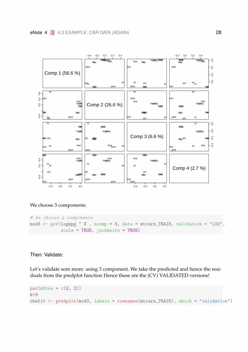
#Loadings:
loadingplot(mod,comps = 1:4, scatter = TRUE, labels = names(mtcars_TRAIN))
eNote 4 4.3 EXAMPLE: CAR DATA (AGAIN) 28
Comp 1 (56.6 %)
−0.4 −0.2 0.0 0.2 0.4
mpgcyldisp
hp
drat
wt
qsecvsam
gear
carblogmpgX
train
mpgcyldisp
hp
drat
wt
qsecvsam
gear
carblogmpgX
train
−0.2 0.0 0.2 0.4
−0.
20.
00.
20.
4mpg cyldisp
hp
drat
wt
qsecvsam
gear
carb logmpgX
train
−0.
40.
00.
20.
4
mpgcyl
disphp
drat
wt
qsec
vsamgear
carblogmpg
Xtrain
Comp 2 (26.6 %) mpgcyl
disphp
drat
wt
qsec
vsamgear
carblogmpg
Xtrain
mpgcyl
disp hp
drat
wt
qsec
vsamgear
carblogmpg
X train
mpg
cyl
disphp
dratwtqsec
vs
am
gear
carb
logmpg
Xtrain
mpg
cyl
disphp
drat wtqsec
vs
am
gear
carb
logmpg
Xtrain Comp 3 (6.6 %)
−0.
4−
0.2
0.0
0.2
mpg
cyl
disp hp
dratwtqsec
vs
am
gear
carb
logmpg
X train
−0.2 0.0 0.2 0.4
−0.
20.
20.
4
mpg
cyl
disp
hpdrat
wt
qsec
vs
am
gear
carb
logmpg
X
train
mpg
cyl
disp
hpdrat
wt
qsec
vs
am
gear
carb
logmpg
X
train
−0.4 −0.2 0.0 0.2
mpg
cyl
disp
hpdrat
wt
qsec
vs
am
gear
carb
logmpg
X
train
Comp 4 (2.7 %)
We choose 3 components:
# We choose 4 components
mod3 <- pcr(logmpg ~ X , ncomp = 3, data = mtcars_TRAIN, validation = "LOO",
scale = TRUE, jackknife = TRUE)
Then: Validate:
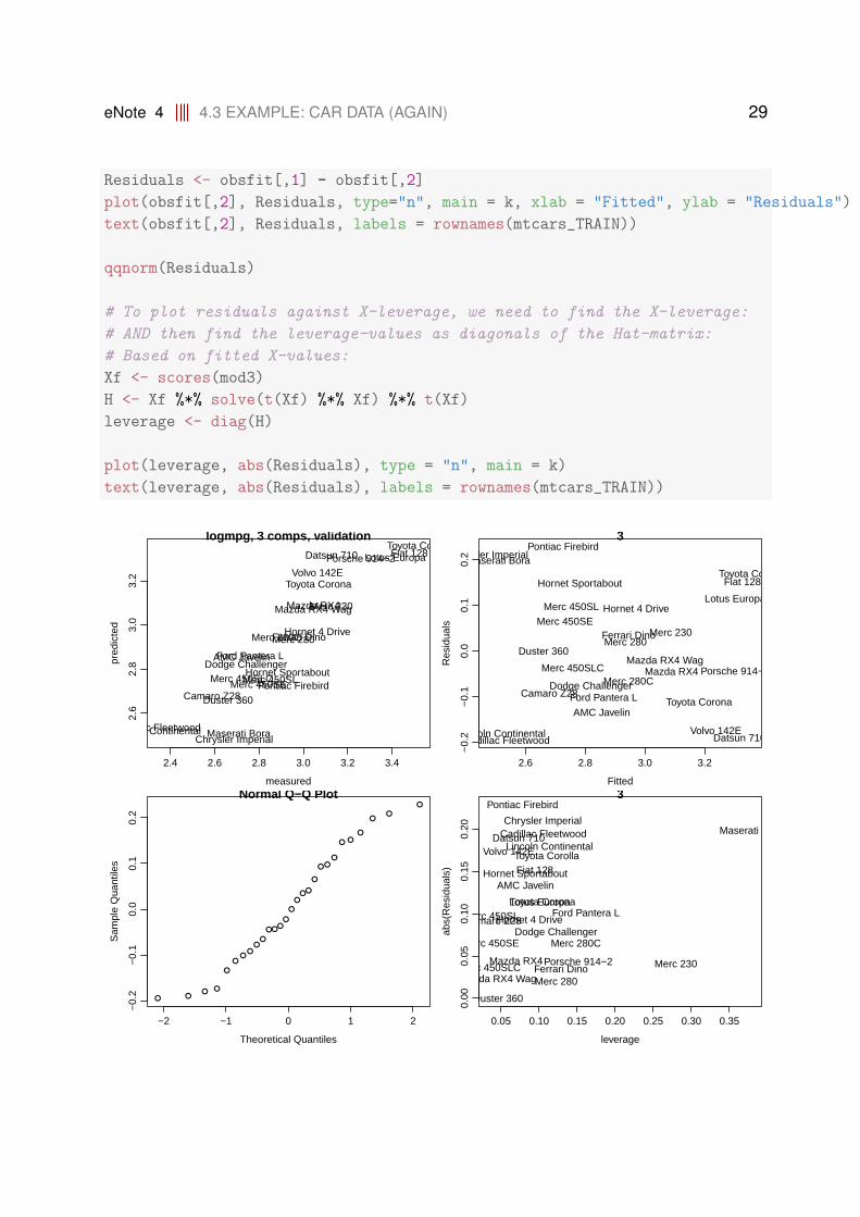
Let’s validate som more: using 3 component. We take the predicted and hence the resi-duals from the predplot function Hence these are the (CV) VALIDATED versions!
par(mfrow = c(2, 2))
k=3
obsfit <- predplot(mod3, labels = rownames(mtcars_TRAIN), which = "validation")
eNote 4 4.3 EXAMPLE: CAR DATA (AGAIN) 29
Residuals <- obsfit[,1] - obsfit[,2]
plot(obsfit[,2], Residuals, type="n", main = k, xlab = "Fitted", ylab = "Residuals")
text(obsfit[,2], Residuals, labels = rownames(mtcars_TRAIN))
qqnorm(Residuals)
# To plot residuals against X-leverage, we need to find the X-leverage:
# AND then find the leverage-values as diagonals of the Hat-matrix:
# Based on fitted X-values:
Xf <- scores(mod3)
H <- Xf %*% solve(t(Xf) %*% Xf) %*% t(Xf)
leverage <- diag(H)
plot(leverage, abs(Residuals), type = "n", main = k)
text(leverage, abs(Residuals), labels = rownames(mtcars_TRAIN))
2.4 2.6 2.8 3.0 3.2 3.4
2.6
2.8
3.0
3.2
logmpg, 3 comps, validation
measured
pred
icte
d
Mazda RX4Mazda RX4 Wag
Datsun 710
Hornet 4 Drive
Hornet Sportabout
Duster 360
Merc 230
Merc 280Merc 280C
Merc 450SEMerc 450SLMerc 450SLC
Cadillac FleetwoodLincoln ContinentalChrysler Imperial
Fiat 128Toyota Corolla
Toyota Corona
Dodge ChallengerAMC Javelin
Camaro Z28Pontiac Firebird
Porsche 914−2Lotus Europa
Ford Pantera L
Ferrari Dino
Maserati Bora
Volvo 142E
2.6 2.8 3.0 3.2
−0.
2−
0.1
0.0
0.1
0.2
3
Fitted
Res
idua
ls
Mazda RX4Mazda RX4 Wag
Datsun 710
Hornet 4 Drive
Hornet Sportabout
Duster 360
Merc 230Merc 280
Merc 280C
Merc 450SEMerc 450SL
Merc 450SLC
Cadillac FleetwoodLincoln Continental
Chrysler Imperial
Fiat 128Toyota Corolla
Toyota Corona
Dodge Challenger
AMC Javelin
Camaro Z28
Pontiac Firebird
Porsche 914−2
Lotus Europa
Ford Pantera L
Ferrari Dino
Maserati Bora
Volvo 142E
●
●
●
●
●
●
●
●
●
●
●
●
●●
●
●●
●
●
●
●
●
●
●
●
●
●
●
−2 −1 0 1 2
−0.
2−
0.1
0.0
0.1
0.2
Normal Q−Q Plot
Theoretical Quantiles
Sam
ple
Qua
ntile
s
0.05 0.10 0.15 0.20 0.25 0.30 0.35
0.00
0.05
0.10
0.15
0.20
3
leverage
abs(
Res
idua
ls)
Mazda RX4
Mazda RX4 Wag
Datsun 710
Hornet 4 Drive
Hornet Sportabout
Duster 360
Merc 230
Merc 280
Merc 280CMerc 450SE
Merc 450SL
Merc 450SLC
Cadillac FleetwoodLincoln Continental
Chrysler Imperial
Fiat 128Toyota Corolla
Toyota Corona
Dodge Challenger
AMC Javelin
Camaro Z28
Pontiac Firebird
Porsche 914−2
Lotus EuropaFord Pantera L
Ferrari Dino
Maserati Bora
Volvo 142E
eNote 4 4.3 EXAMPLE: CAR DATA (AGAIN) 30
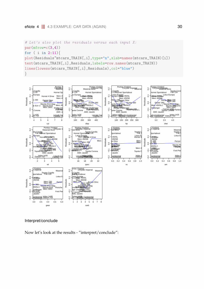
# Let’s also plot the residuals versus each input X:
par(mfrow=c(3,4))
for ( i in 2:11){plot(Residuals~mtcars_TRAIN[,i],type="n",xlab=names(mtcars_TRAIN)[i])
text(mtcars_TRAIN[,i],Residuals,labels=row.names(mtcars_TRAIN))
lines(lowess(mtcars_TRAIN[,i],Residuals),col="blue")
}
4 5 6 7 8
−0.
2−
0.1
0.0
0.1
0.2
cyl
Res
idua
ls
Mazda RX4Mazda RX4 Wag
Datsun 710
Hornet 4 Drive
Hornet Sportabout
Duster 360
Merc 230Merc 280
Merc 280C
Merc 450SEMerc 450SL
Merc 450SLC
Cadillac FleetwoodLincoln Continental
Chrysler Imperial
Fiat 128Toyota Corolla
Toyota CoronaDodge Challenger
AMC Javelin
Camaro Z28
Pontiac Firebird
Porsche 914−2
Lotus Europa
Ford Pantera L
Ferrari Dino
Maserati Bora
Volvo 142E
100 200 300 400
−0.
2−
0.1
0.0
0.1
0.2
disp
Res
idua
ls
Mazda RX4Mazda RX4 Wag
Datsun 710
Hornet 4 Drive
Hornet Sportabout
Duster 360
Merc 230Merc 280
Merc 280C
Merc 450SEMerc 450SL
Merc 450SLC
Cadillac FleetwoodLincoln Continental
Chrysler Imperial
Fiat 128Toyota Corolla
Toyota CoronaDodge Challenger
AMC Javelin
Camaro Z28
Pontiac Firebird
Porsche 914−2
Lotus Europa
Ford Pantera L
Ferrari Dino
Maserati Bora
Volvo 142E
100 150 200 250 300
−0.
2−
0.1
0.0
0.1
0.2
hp
Res
idua
lsMazda RX4
Mazda RX4 Wag
Datsun 710
Hornet 4 Drive
Hornet Sportabout
Duster 360
Merc 230Merc 280
Merc 280C
Merc 450SEMerc 450SL
Merc 450SLC
Cadillac FleetwoodLincoln Continental
Chrysler Imperial
Fiat 128Toyota Corolla
Toyota CoronaDodge Challenger
AMC Javelin
Camaro Z28
Pontiac Firebird
Porsche 914−2
Lotus Europa
Ford Pantera L
Ferrari Dino
Maserati Bora
Volvo 142E
3.0 3.5 4.0
−0.
2−
0.1
0.0
0.1
0.2
drat
Res
idua
ls
Mazda RX4Mazda RX4 Wag
Datsun 710
Hornet 4 Drive
Hornet Sportabout
Duster 360
Merc 230Merc 280
Merc 280C
Merc 450SEMerc 450SL
Merc 450SLC
Cadillac FleetwoodLincoln Continental
Chrysler Imperial
Fiat 128Toyota Corolla
Toyota CoronaDodge Challenger
AMC Javelin
Camaro Z28
Pontiac Firebird
Porsche 914−2
Lotus Europa
Ford Pantera L
Ferrari Dino
Maserati Bora
Volvo 142E
2 3 4 5
−0.
2−
0.1
0.0
0.1
0.2
wt
Res
idua
ls
Mazda RX4Mazda RX4 Wag
Datsun 710
Hornet 4 Drive
Hornet Sportabout
Duster 360
Merc 230Merc 280
Merc 280C
Merc 450SEMerc 450SL
Merc 450SLC
Cadillac FleetwoodLincoln Continental
Chrysler Imperial
Fiat 128Toyota Corolla
Toyota CoronaDodge Challenger
AMC Javelin
Camaro Z28
Pontiac Firebird
Porsche 914−2
Lotus Europa
Ford Pantera L
Ferrari Dino
Maserati Bora
Volvo 142E
16 18 20 22
−0.
2−
0.1
0.0
0.1
0.2
qsec
Res
idua
ls
Mazda RX4Mazda RX4 Wag
Datsun 710
Hornet 4 Drive
Hornet Sportabout
Duster 360
Merc 230Merc 280
Merc 280C
Merc 450SEMerc 450SL
Merc 450SLC
Cadillac FleetwoodLincoln Continental
Chrysler Imperial
Fiat 128Toyota Corolla
Toyota CoronaDodge Challenger
AMC Javelin
Camaro Z28
Pontiac Firebird
Porsche 914−2
Lotus Europa
Ford Pantera L
Ferrari Dino
Maserati Bora
Volvo 142E
0.0 0.2 0.4 0.6 0.8 1.0
−0.
2−
0.1
0.0
0.1
0.2
vs
Res
idua
ls
Mazda RX4Mazda RX4 Wag
Datsun 710
Hornet 4 Drive
Hornet Sportabout
Duster 360
Merc 230Merc 280
Merc 280C
Merc 450SEMerc 450SL
Merc 450SLC
Cadillac FleetwoodLincoln Continental
Chrysler Imperial
Fiat 128Toyota Corolla
Toyota CoronaDodge Challenger
AMC Javelin
Camaro Z28
Pontiac Firebird
Porsche 914−2
Lotus Europa
Ford Pantera L
Ferrari Dino
Maserati Bora
Volvo 142E
0.0 0.2 0.4 0.6 0.8 1.0
−0.
2−
0.1
0.0
0.1
0.2
am
Res
idua
lsMazda RX4
Mazda RX4 Wag
Datsun 710
Hornet 4 Drive
Hornet Sportabout
Duster 360
Merc 230Merc 280
Merc 280C
Merc 450SEMerc 450SL
Merc 450SLC
Cadillac FleetwoodLincoln Continental
Chrysler Imperial
Fiat 128Toyota Corolla
Toyota CoronaDodge Challenger
AMC Javelin
Camaro Z28
Pontiac Firebird
Porsche 914−2
Lotus Europa
Ford Pantera L
Ferrari Dino
Maserati Bora
Volvo 142E
3.0 3.5 4.0 4.5 5.0
−0.
2−
0.1
0.0
0.1
0.2
gear
Res
idua
ls
Mazda RX4Mazda RX4 Wag
Datsun 710
Hornet 4 Drive
Hornet Sportabout
Duster 360
Merc 230Merc 280
Merc 280C
Merc 450SEMerc 450SL
Merc 450SLC
Cadillac FleetwoodLincoln Continental
Chrysler Imperial
Fiat 128Toyota Corolla
Toyota CoronaDodge Challenger
AMC Javelin
Camaro Z28
Pontiac Firebird
Porsche 914−2
Lotus Europa
Ford Pantera L
Ferrari Dino
Maserati Bora
Volvo 142E
1 2 3 4 5 6 7 8
−0.
2−
0.1
0.0
0.1
0.2
carb
Res
idua
ls
Mazda RX4Mazda RX4 Wag
Datsun 710
Hornet 4 Drive
Hornet Sportabout
Duster 360
Merc 230Merc 280
Merc 280C
Merc 450SEMerc 450SL
Merc 450SLC
Cadillac FleetwoodLincoln Continental
Chrysler Imperial
Fiat 128Toyota Corolla
Toyota CoronaDodge Challenger
AMC Javelin
Camaro Z28
Pontiac Firebird
Porsche 914−2
Lotus Europa
Ford Pantera L
Ferrari Dino
Maserati Bora
Volvo 142E
Interpret/conclude
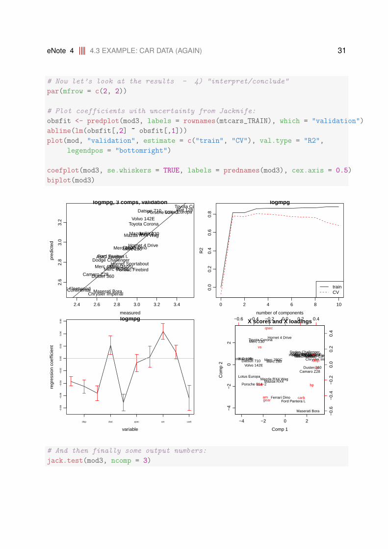
Now let’s look at the results - ”interpret/conclude”:
eNote 4 4.3 EXAMPLE: CAR DATA (AGAIN) 31
# Now let’s look at the results - 4) "interpret/conclude"
par(mfrow = c(2, 2))
# Plot coefficients with uncertainty from Jacknife:
obsfit <- predplot(mod3, labels = rownames(mtcars_TRAIN), which = "validation")
abline(lm(obsfit[,2] ~ obsfit[,1]))
plot(mod, "validation", estimate = c("train", "CV"), val.type = "R2",
legendpos = "bottomright")
coefplot(mod3, se.whiskers = TRUE, labels = prednames(mod3), cex.axis = 0.5)
biplot(mod3)
2.4 2.6 2.8 3.0 3.2 3.4
2.6
2.8
3.0
3.2
logmpg, 3 comps, validation
measured
pred
icte
d
Mazda RX4Mazda RX4 Wag
Datsun 710
Hornet 4 Drive
Hornet Sportabout
Duster 360
Merc 230
Merc 280Merc 280C
Merc 450SEMerc 450SLMerc 450SLC
Cadillac FleetwoodLincoln ContinentalChrysler Imperial
Fiat 128Toyota Corolla
Toyota Corona
Dodge ChallengerAMC Javelin
Camaro Z28Pontiac Firebird
Porsche 914−2Lotus Europa
Ford Pantera L
Ferrari Dino
Maserati Bora
Volvo 142E
0 2 4 6 8 10
0.0
0.2
0.4
0.6
0.8
logmpg
number of components
R2
trainCV
−0.
08−
0.06
−0.
04−
0.02
0.00
0.02
0.04
0.06 logmpg
variable
regr
essi
on c
oeffi
cien
t
disp drat qsec am carb −4 −2 0 2
−4
−2
02
X scores and X loadings
Comp 1
Com
p 2
Mazda RX4Mazda RX4 Wag
Datsun 710
Hornet 4 Drive
Hornet Sportabout
Duster 360
Merc 230
Merc 280Merc 280CMerc 450SEMerc 450SLMerc 450SLCCadillac FleetwoodLincoln Continental
Chrysler ImperialFiat 128Toyota Corolla
Toyota Corona
Dodge ChallengerAMC Javelin
Camaro Z28
Pontiac Firebird
Porsche 914−2
Lotus Europa
Ford Pantera LFerrari Dino
Maserati Bora
Volvo 142E
−0.6 −0.4 −0.2 0.0 0.2 0.4
−0.
6−
0.4
−0.
20.
00.
20.
4
cyl
disp
hpdrat
wt
qsec
vs
amgear
carb
# And then finally some output numbers:
jack.test(mod3, ncomp = 3)
eNote 4 4.3 EXAMPLE: CAR DATA (AGAIN) 32
Response logmpg (3 comps):
Estimate Std. Error Df t value Pr(>|t|)
cyl -0.0366977 0.0077887 27 -4.7116 6.611e-05 ***
disp -0.0452754 0.0108002 27 -4.1921 0.0002658 ***
hp -0.0557347 0.0118127 27 -4.7182 6.495e-05 ***
drat 0.0213254 0.0149417 27 1.4272 0.1649761
wt -0.0707133 0.0134946 27 -5.2401 1.598e-05 ***
qsec -0.0073511 0.0137758 27 -0.5336 0.5979674
vs 0.0028425 0.0168228 27 0.1690 0.8670842
am 0.0436837 0.0128767 27 3.3925 0.0021513 **
gear 0.0104731 0.0109513 27 0.9563 0.3473857
carb -0.0635746 0.0198725 27 -3.1991 0.0035072 **
---
Signif. codes: 0 ’***’ 0.001 ’**’ 0.01 ’*’ 0.05 ’.’ 0.1 ’ ’ 1
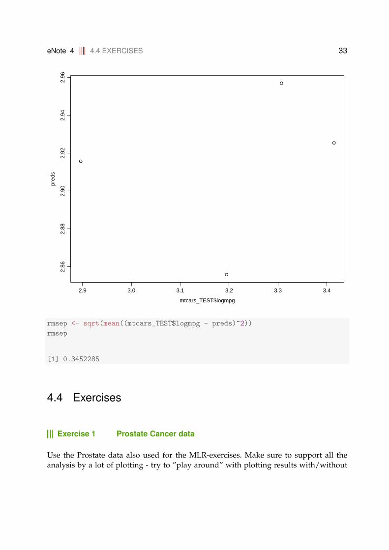
Prediction
# And now let’s try to predict the 4 data points from the TEST set:
preds <- predict(mod3, newdata = mtcars_TEST, comps = 3)
plot(mtcars_TEST$logmpg, preds)
eNote 4 4.4 EXERCISES 33
●
●
●
●
2.9 3.0 3.1 3.2 3.3 3.4
2.86
2.88
2.90
2.92
2.94
2.96
mtcars_TEST$logmpg
pred
s
rmsep <- sqrt(mean((mtcars_TEST$logmpg - preds)^2))
rmsep
[1] 0.3452285
4.4 Exercises
Exercise 1 Prostate Cancer data
Use the Prostate data also used for the MLR-exercises. Make sure to support all theanalysis by a lot of plotting - try to ”play around” with plotting results with/without

eNote 4 4.4 EXERCISES 34
extreme observations. Also try to look at results for different choices of number of com-ponents (to get a feeling for the consequence of that). The Rcode (including comments)for the Leslie Salt data above can be used as a template for a good approach.
a) Define test sets and training sets according to the last column in the data set. DoPCR on the training set – use cross-validation. Go through ALL the relevant steps:
1. model selection
2. validation
3. interpretation
4. etc.
b) Predict the test set lpsa values. What is the average prediction error for the testset?
c) Compare with the cross validation error in the training set - try both ”LOO”and asegmented version of CV
d) Compare with an MLR prediction using ALL predictors