a comparison of approaches to stepwise regression on

Accepted refereed manuscript of: Wang M, Wright J, Brownlee A & Buswell R (2016) A comparison of approaches to stepwise regression on variables sensitivities in building simulation and analysis, Energy and Buildings, 127, pp. 313-326. DOI: 10.1016/j.enbuild.2016.05.065

© 2016, Elsevier. Licensed under the Creative Commons Attribution-NonCommercial-NoDerivatives 4.0 International http://creativecommons.org/licenses/by-nc-nd/4.0/

http://dx.doi.org/10.1016/j.enbuild.2016.05.065

http://creativecommons.org/licenses/by-nc-nd/4.0/

A COMPARISON OF APPROACHES TO STEPWISE REGRESSION ON

VARIABLES SENSITIVITIES IN BUILDING SIMULATION AND

ANALYSIS

Mengchao Wang1, Jonathan Wright1, Alexander Brownlee2, Richard Buswell1

1School of Civil &Building Engineering, Loughborough University, Loughborough, LE11 3TU, UK. 2Computing Science &Mathematics, University of Stirling, Stirling, FK9 4LA, UK.

Highlights:

The robustness of stepwise regression is irrespective of selection approach. The linear regression model constructed by AIC has a high risk of overfitting,

especially when the sample size is small. A mixture of discretized-continuous and categorical variables can be used for

global SA. For stepwise regression, increasing sample size can identify more sensitive

variables, but the importance of highly sensitive variables remains the same. The importance of variables for design objectives and constraints is better to

be classified through more than one sensitivity indexes.

Abstract

Developing sensitivity analysis (SA) that reliably and consistently identify sensitive

variables can improve building performance design. In global SA, a linear regression

model is normally applied to sampled-based solutions by stepwise manners, and the

relative importance of variables is examined by sensitivity indexes. However, the

robustness of stepwise regression is related to the choice of procedure options, and

therefore influence the indication of variables’ sensitivities. This paper investigates the

extent to which the procedure options of a stepwise regression for design objectives or

constraints can affect variables global sensitivities, determined by three sensitivity

indexes. Given that SA and optimization are often conducted in parallel, desiring for a

combined method, the paper also investigates SA using both randomly generated

samples and the biased solutions obtained from an optimization run. Main contribution

is that, for each design objective or constraint, it is better to conclude the categories of

variables importance, rather than ordering their sensitivities by a particular index.

Importantly, the overall stepwise approach (with the use of bidirectional elimination,

BIC, rank transformation and 100 sample size) is robust for global SA: the most

important variables are always ranked on the top irrespective of the procedure options.

Keywords: Global sensitivity analysis, Stepwise regression, Sensitivity indexes,

Standardized (rank) regression coefficients.

1. Introduction

Reducing the energy consumption in the building sector have a critical role in meeting

energy and emission reduction targets in both developing and developed countries [15,

21]. In order to improve building performance by implementing the optimal design

solutions at a reasonable investment, both sensitivity analysis and model-based

optimization can be used to inform design decisions. Compared to model-based

optimization that is applied to find the combinations of variables values that optimize

the objectives while satisfying the design constraints, Monte Carlo sensitivity analysis

(SA) can support decision making by providing insight into the input variables that

most influence design objectives, such as operational energy use or comfort metrics of

the final building [16, 24]. This makes SA a useful tool for designers. Consequently,

developing SA methodologies that reliably and consistently identify sensitive variables

is an important area of research.

SA can be generally grouped into local and global forms [23]. Global SA based on a

linear regression is normally adopted to evaluate the relative importance of input

variables [2, 3, 12]. When many input variables are involved, stepwise regression

provides an alternative. Saltelli et al. [23] state that, when the input variables are ideally

uncorrelated, the importance of variables sorted by any sensitivity indexes should be

the same. This applies whether sorting by: order of addition to the regression model;

size of the R2 changes attributable to individual variables; absolute values of variables’

standardized (rank) regression coefficients (SRCs/SRRCs); absolute values of

correlations coefficients (CCs); or absolute values of partial correlation coefficients

(PCCs). Therefore, in previous researches, the global sensitivities of variables are

normally evaluated by a particular index, e.g. De Wilde et al. [7] using SRRCs to

determine the major contributors for heating energy use; Hopfe and Hensen [16] using

both SRRCs and the change of R2 to explore variables influence on building

performance simulation.

However, according to our previous researches [27, 28], the ordering of variables’

importance with respect to design objectives and constraints could be switched by

applying the same global SA method to different sets of random samples. Furthermore,

the robustness and effectiveness of a stepwise regression depends on the choice of

procedure options, as each option has its advantages and weakness [26]. For instance,

the F-test is often used as default criterion to stop the stepwise regression process, but

it has been shown to perform poorly relative to other criteria, e.g. the corrected AIC

[17]. It has also been shown that it is possible to conduct global SA in parallel with

optimization by an evolutionary algorithm [25]. This further supports decision making

by providing suggested optimal solutions as well as variables’ sensitivities. Solutions

generated during the optimization run can be reused for the global SA to save

computational efforts, despite the bias in the samples arising from operation of the

evolutionary algorithm.

Therefore, this paper explores the impact of procedure options in a global SA for design

objectives or constraints, providing insights that will enable more robust and more

accurate assessments of variables’ sensitivities to be made, through the relative

magnitudes of variables sensitivity indexes. The procedure options explored are:

different approaches to obtaining samples (i.e. randomly generated samples or the

biased solutions obtained at the start of an optimization process, with a sample size of

100 or 1000); data forms of input variables (i.e. raw data with categorical variables, or

rank-transformed data); selection approaches (i.e. the results in this paper are based on

bidirectional elimination); and selection criteria (i.e. F-test, AIC or BIC).

2. Stepwise Regression Methodology

Stepwise regression analysis is usually used as an alternative of linear regression to do

global SA. Since, when no impacted or correlated variables are included in the same

regression model, it can avoid misleading regression of variables importance. It can

also avoid overfitting of the data, as all of input variables are arbitrarily forced into the

same regression model [23]. Overfitting occurs when the regression model in essence

‘chases’ the individual observations rather than following an overall pattern in the data,

which can produce a spurious model, giving poor predictions of variables importance

[23]. Thus, the overfitting is used as an important standard, to evaluate how well the

linear model constructed by stepwise regression can fit to the data (generated from

different samples).

Therefore, the global SA adopted here is based on a linear regression model in the

stepwise manner, which is performed by R statistic software [20]. The idea is to add or

remove variables in a linear model: at each iteration, selecting the variable which most

increases the R2 coefficient of the model. The robustness of stepwise regression

analysis is dependent on the choice of procedure options, including the sampling

method, sample size, data form of input variables, selection approach and selection

criterion, with the accuracy being evaluated through the R2 (coefficient of

determination) and PRESS (predicted error sum of squares) values in the linear

regression model.

In a stepwise regression analysis, the relative importance of the variables for a given

output can be evaluated through sensitivity indexes, including variables’ entry-order to

the model, SRCs (standardized regression coefficients)/SRRCs (standardized rank

regression coefficients, for rank-transformed data), and R2 change attributable to the

individual variables. The more important (sensitive) the variable is, the earlier it is

selected into the linear model, the larger its SRC/SRRC is, the greater it is attributable

to R2 change [23].

2.1 Samples and sample size

The robustness of a sensitivity method is related to the choice of sample size and the

manner in which the samples are generated [23]. For a sample size of 100 and above,

the difference in the results from different sampling methods is decreased; thus, it is

feasible to use a random sampling method and 100 samples in a Monte Carlo analysis

for typical building simulation applications [19, 22]. In this paper, the conclusion is

further validated by comparing the SA resulting from a 100 random samples with those

from a 1000 random samples; the 100 random samples are taken as being the first 100

samples of the 1000 randomly generated samples. The repeatability of the approach is

investigated by repeating the analysis for two sets of random samples (Random Sample

A and Random Sample B). Moreover, the first 100 solutions (being consistent with the

smaller sample size in random samples) obtained from a multi-objective optimization

process (based on NSGA-II) have also been used to do global SA, for design objectives

and constraints (See Section 3.1). The aim is to explore the extent to which the biased

samples can affect the robustness of variables global sensitivities, determined by the

same method based on stepwise regression.

2.2 Input variables and rank-transformation

The input variables considered in most sensitivity analyses are real-valued quantities

[14, 16]. However, in this paper, the categorical variables for construction types are

applied with others having physical representations (see Section 4.1). Such variables

frequently appear in building design problems, so it is important to consider them.

Furthermore, a non-linear relationship between the input variables and the output is

possible, whether the input variables have real-valued quantities or not. A rank

transformation of the variables based on a monotonic relationship can mitigate the

problems associated with fitting linear models to nonlinear data [23]. The rank

transformation is defined according to Spearman’s rank correlation coefficients: raw

data are replaced by their corresponding ranks, and then the ranks of input variables

and outputs are used to do regression analysis. Particularly, the smallest rank 1 is

assigned to the smallest value of each variable, and then the rank 2 is assigned to the

next larger value, and so on until the largest rank m assigned to the largest value (i.e. m

indicates the number of observations for each variable).

Thus, two alternative representations of the input variables are considered here:

The input variables in their raw form.

A rank-transformation of the variables (and outputs).

2.3 Selection approach

There are three model-selection approaches [6] as below. Due to identical results in this

case study, the results from bidirectional elimination are only discussed here:

Forward selection: which starts from an ‘empty’ model with no input variable

but an intercept, and then adds the variable most improving the model one-at-

a-time until no more added variables can significantly improve the model. This

approach is based on a pre-defined selection criterion.

Backward elimination: which starts from a ‘full’ model with all predictive input

variables and an intercept, and then deletes the variable least improving the

model one-at-a-time until no more deleted variables can significantly improve

the model. This approach is based on a pre-selected selection criterion.

Bidirectional elimination: which is essentially a forward selection procedure but

with the possibility of deleting a selected variable at each stage, as in the

backward elimination. This approach is commonly applied for stepwise

regression, particularly when there are correlations between variables.

2.4 Selection criterion

The selection criterion is used to stop the construction of the stepwise regression. It is

also used to determine when an already-selected variable should be deleted from the

linear regression model. The commonly applied selection criteria that are adopted in

this research are:

F-test: which is often used as a default criterion for stepwise regression. To

avoid overfitting the model, Saltelli et al. [23] suggest using the α-value of 0.01

or 0.02 for a F-test, rather than the conventional choice of 0.05.

AIC (Akaike information criterion): which is based on a penalty of maximum

log likelihood (the maximum likelihood is defined as a general technique to

estimate the parameters and draw statistical inferences in various situations,

especially in non-standard ones), to balance the linearity of the model with the

model size [13].

BIC (Bayesian information criterion): which is an alternative method to AIC.

In comparison to AIC, it penalizes larger model models more heavily, aiming

to avoid the overfitting problem.

This research focuses on comparing the robustness of stepwise regression driven by

AIC and BIC. The linear regression models selected by F-test (with different α-values

of 0.01, 0.02 or 0.05) are primarily used to examine the influences of the selection

criterion on the overfitting problem.

2.5 Model accuracy

The adequacy of a linear regression model’s fit can be assessed through R2 (coefficient

of determination) and PRESS (predicted error sum of squares) [23], which are both

considered in this paper:

R2 (coefficient of determination): is a simple way to test the linear fitness of a

model, having a value between zero and unity: the larger the R2 value is, the

better the model fits the data. In this paper, a fairly strong linear regression

model is valid for the value of R2 >0.7.

PRESS (predicted error sum of squares): the value of which can be used to

check the model 'overfitting' to the data. According to Satelli et al. (2008),

overfitting could occur when the regression model involving more variables, in

essence it ‘chases’ the individual observations rather than following an overall

pattern in the data, which can produce a spurious model, giving poor predictions

of variables importance. In particular, when a variable has been added into the

model, resulting in an increased PRESS value, the model is overfitted.

Therefore, the linear regression model with the lowest PRESS value is preferred

when choosing between two competing regression models.

3. Experimental Approach

3.1 Multi-objective optimization algorithm

Evolutionary algorithms (EAs) have been shown to perform well for many building

optimization problems [11]. Their origins are based on Darwinian principles: survival

of the fittest population of solution, passing of characteristics from parents to offspring,

and eliminating of the poorest solution during each generation. Building design

problems are inherently multi-objective, where the designer seeks to find an optimal

trade-off between two or more conflicting design criteria. Consequently, this work

adopts the well-known non-dominated sorting genetic algorithm II (NSGA-II) [8],

which is used widely to solve bi- and multi-objective building optimization problems

[4, 11]. The algorithm is an EA which seeks to approximate the Pareto front of solutions

that represents the trade-off in the optimization objectives. The specific implementation

of NSGA-II is:

Gray-coded bit-string encoding of the problem variables (163 bits);

uniform crossover (100% probability of chromosome crossover with 50%

probability of gene crossover);

single bit mutation (a probability of 1 bit per chromosome);

passive archive of solutions, allowing a Pareto front to be constructed from all

solutions visited during the search rather than only those in the final population;

population size of 20 with the search stopped after 5000 unique simulations.

These parameters were chosen empirically.

3.2 Example Building and HVAC Systems

The example building is based on a mid-floor of a commercial office building with 5

zones located in Birmingham, England (Figures 1 and 2). The size of two end zones

and three middle zones are 24m x 8m and 30m x 8m separately, with floor to ceiling

height of 2.7m. Each zone has typical design conditions of 1 occupant per 10m2 floor

area and equipment loads of 11.5 W/m2 floor area. Maximum lighting loads are set at

11.5 W/m2 floor area, with the lighting output controlled to provide an illuminance of

500 lux at two reference points located in each of the perimeter zones. Infiltration is set

at 0.1 air change per hour and ventilation rates at 8 l/s per person. The heating and

cooling is modelled by an idealised system that can provide sufficient energy to offset

the zone loads and meet the zone temperature setpoint during hours of operation (from

9am to 5pm all year around). The internal zone is treated as a passive unconditioned

space. The operational energy use, building comfort, and the capital costs related to

equipment size, are determined by EnergyPlus [9], with the weather data based on the

CIBSE reference year [5].

4 Input Variables, Objective Functions and Design Constraints

4.1 Input variables characteristics

Table 1 gives 16 input variables, and specifies their bounds, discrete increment, and

the total number of unique value that each can take, according to model characteristics,

previous experiments and handbooks [1, 10]. Those input variables associated with

perimeter zones are related to building geometry (i.e. orientation and window-wall

ratios), the properties of constructions (i.e. window/wall/ceiling-floor types), and

operating conditions (i.e. heating and cooling setpoint (via the dead band), system

operating hours (per day) in ‘winter’ months (November to April) and ‘summer’

months (May to October) (via winter/summer start and stop time)).

The longest façades of the building face the ‘true north/south’, when the variable of

orientation is set at 0o. For the example building, the valid value range of orientation

is -90o to 90o. In order to avoid an overlap of the heating and cooling setpoint, dead

band is used instead of the cooling setpoint, even the heating and cooling have the

potential to be run all year around [10]. The window-wall ratio refers to the window

area of 6 equally sized windows placed in three groups against the wall area in each

façade (see Figures 1 and 2): its value range for this case-study building is between 0.2

and 0.9. The façade-1/2/3/4 window-wall ratio reflects its position in each perimeter

zone, corresponding to Zone N/S/E/W. Both heating and cooling are available all year

around, although the operating hours (between start and stop time) are different for the

‘winter’ months (November to April) and ‘summer’ months (May to October) [10].

Three construction types are available for external wall and ceiling-floor constructions:

heavy weight, medium weight and lightweight. Similarly, there are two internal wall

types (heavy weight and light weight), and two double-glazed windows types (plain

glass and low-emissivity (Low-E) glass). For categorical construction variables, the

heavy weight construction corresponds to a value of 0, with the construction weight

decreasing with increasing variable value; for window type, the normal plain and Low-

E glasses are corresponding to the values of 0 and 1 separately [1]. Since, based on

previous researches [25], the construction variables having physical representation or

having not barely affect the performance of stepwise regression (i.e. the identification

of variables importance to output), and in a real case, the combination of variables is

normally mixed with different data types (continued, discrete or categorical variables).

In this paper, no prior knowledge of variable sensitivity is assumed. Thus, in a set of

randomly generated samples, the frequency distributions of variables are uniform and

the correlations between any pairs of variables are less than 0.1.

4.2 Design objectives and constraints

The design objectives, to be minimised by a multi-objective optimization process, are

the building annual energy demand (as determined by EnergyPlus (V7) for heating,

cooling and artificial lighting), and the capital costs (using a model derived from cost

estimating data in London, UK [18]):

Energy demand: the annual energy demand of the heating, cooling and

artificial lighting. As the HVAC system of the example building is an ideal load

air system, it is not like the real case where the cooling energy could be reduced

to ‘free’, due to the free cooling ventilation. The ‘energy consumption’ is more

correctly defined as ‘energy demand’ in this paper.

Capital costs: is known to be a linear function of most of the variables, although

the cost of the HVAC system is a function of the peak heating and cooling

capacity, the capacity being a non-linear function of some variables.

The design constraints are that the thermal comfort in each perimeter zone should not

exceed 20% of predicted percentage dissatisfied (PPD), for no more than 150 working

hours per annum. The constraint functions are configured to return the number of hour

above 150, or zero if the constraint is feasible. The solution infeasibility combines the

separate constraint violations into a single metric. It is taken as the sum of the squares

of each constraint violation (with an entirely feasible solution having an infeasibility of

zero). Thus, the infeasibility only has a non-zero value when one or more constraints

are violated (this forming a discontinuity in the function space, with the infeasibility of

the infeasible solutions changing with the variable values, but all feasible solutions

having a constant infeasibility of zero). For randomly generated solutions, most of the

solutions are infeasible.

5. Results and Analysis

5.1 The impact of selection approach

In this paper, for each set of samples (random and slightly biased samples from

optimization), the linear regression models driven by different selection approaches are

identical, represented in terms of the number of variables involved in the model (i.e.

the size of the model), and the R2 and PRESS values. Therefore, the selection approach

(forward, backward, or bidirectional) has no impact on the identification and

determination of variables sensitivities (represented by sensitivity indexes of variables

entry-orders, SRCs/SRRCs and the change of R2), for design objectives and constraints,

although variables could be moderately correlated (i.e. the maximum correlation

coefficients between variables are approximate 0.55, when the first 100 optimization

solutions are taken from the NSGA-II search). As the linear regression model

constructed by the backward elimination only removes variables with no impact from

the full model, it is meaningless to sort variables importance based on their entry-orders

or individual contributions to R2 change. In this paper, the results from stepwise

regression with the use of bidirectional elimination are only presented as it is a

combination of the two other selection approaches.

5.2 The impact of selection criterion

Figure 3 compares the fitness of the linear regression models for energy demand, capital

costs and solution infeasibility, that were constructed by different selection criteria (i.e.

AIC, BIC, and F-test with α-level of 0.05, 0.02 or 0.01) using global SA with raw and

rank-transformed data from 5 different sets of samples. These were the 100 and 1000

randomly generated solutions from Random Sample A and Random Sample B, and the

first 100 biased solutions obtained at the beginning of NSGA-II. In order to protect

against overfitting, the regression models with minimum PRESS values are also

included in this figure. Columns exceeding that of minimum PRESS are classed as

overfitted (containing redundant variables). Thus, for a given set of samples

(irrespective of sampling methods and sample size), the number of variables selected

into a linear regression model by a stepwise manner depends on the choice of selection

criterion. The linear regression model constructed by AIC always contains the largest

number of input variables, which increases the risk of overfitting, particularly in the

case of a smaller sample size (e.g. a sample size of 100). In contrast, the performance

of F-test is relevant to the choice of significance level (α-value): the global SA driven

by F-test with α-value of 0.01 or 0.02 is close to that found by BIC, but the F-test with

α-value of 0.05 performs close to that of AIC. In this case study, the regression models

constructed by BIC, F-test with α-value of 0.01, 0.02 or 0.05, and AIC with larger

sample size (i.e. 1000) do not cause overfitting problems in the global SA.

Furthermore, the differences between AIC and BIC on the determination of variables’

sensitivity have also been evaluated, and are given in Tables 2 and 3. These show the

percentage changes in variables sensitivity indexes; that is, the percentage changes of

the sensitivity indexes for variables identified by BIC, due to the application of AIC.

The length of the bars indicates the relative magnitude of the percentage change: the

larger the bar, the more significant changes due to different selection criteria. It can

conclude that the choice of selection criterion barely impacts on variables’ entry-orders

and contributions to R2 changes, but it does have some influence on the absolute values

of SRCs/SRRCs (particularly for moderately important variables with medium entry-

orders), which may be due to the mathematical assumption of SRCs/SRRCs calculation;

further research is required. Taking the case of Random Sample B as example, with a

sample size 1000 and rank-transformed data for capital costs (Table 3 column 5), most

medium-ranked variables have approximately 30% variation in their relative

magnitudes of SRRCs due to the choice of different selection criteria. In contrast, the

R2 of the linear model is almost constant.

It can conclude from these results as that, for a given set of samples, while different

selection criteria lead to the linear regression models having different numbers of

variables (that could, in turn, further affect the representation of variables sensitivities),

the selection criterion only has a slight influence onmodel’s fitness (the relative

magnitude of R2). This indicates that those newly added-in variables (due to different

selection criteria, e.g. AIC) account for only limited uncertainty of the design objectives

or constraints. Thus, for computer efficiency and model accuracy (to avoid overfitting

problem), it is better to use BIC as selection criterion to stepwise regression analysis.

5.3 The impact of data type of input variables

Based on previous results, to avoid the overfitting problem, the global SA driven by

BIC and bidirectional elimination is used here to further explore the influences of

procedure options (i.e. data representation and sets of samples) of a stepwise regression,

for design objectives and constraints. Tables 4 to 6 state the global sensitivities of

variables, based on different sensitivity indexes (i.e. the order of variables entry into

the linear regression model, the absolute value of SRCs/SRRCs, and the size of R2

changes attributable to individual variables), for energy demand (Table 4), capital costs

(Table 5) and solution infeasibility (Table 6). In each case, the variables are represented

by rank-transformed data or raw data with categorical variables. Each data type of input

variables applied to global SA has 5 sets of samples, including 100 and 1000 solutions

from Random Sample A and also Random Sample B, as well as the first 100 biased

solutions obtained at the beginning of NSGA-II. In those tables, the length of the bar

indicates the relative magnitude of variable’s importance. The more important

(sensitive) the variable, the longer the bars of the SRCs/SRRCs and the size of R2

change, and correspondingly, the shorter the bar of entry-order.

Firstly, even though the categorical variables have fewer options than others, in the case

of applying the global SA to raw data, the categorical variables are not always ranked

highest for design objectives and constraints. From this, it can be determined that any

error in variables’ importance due to the large changes in values for categorical

variables is not substantial. Thus, in this paper, the discretised-continuous and

categorical variables can be used together, avoiding the overrated problem for

categorical variables.

Furthermore, for a given set of samples, whether or not rank transformationis applied

to the variables, the global SA for a particular design objective leads to similar linear

regression models with very close R2, with only a few switches in the sensitivity of

medium-importance variables. For example, in the case of Random Sample B with a

sample size of 1000 for energy demand (Table 4), the entry-order of rank-transformed

variables into the linear model is as same as that with raw data (except the last two add-

in variables, orientation and façade-4 window-wall ratio), with a small difference in R2

of 0.006. However, for the first 100 NSGA-II solutions for capital costs (Table 5), apart

from the top-three variables, the remainder barely have the same entry-orders, which

may be due to the different characteristics of design objectives: the distributions of the

random samples for energy demand and capital costs have patterns; further research is

required.

Finally, in the case of applying the global SA to randomly generated samples for

solution infeasibility (Table 6), using rank transformation in stepwise regression can

mitigate against the problems associated fitting the linear regression model to non-

linear data, which is indicated by the significantly increased R2 (from about 0.6 to above

0.8) and the enlarged number of identified variables. This is because the regression

model with rank-transformed data is based on a monotonic relationship rather than a

linear relationship. However, for the top two most important variables, heating setpoint

and dead band, the indexes of their global sensitivities to solution infeasibility are

slightly affected by the use of rank transformation. This is represented by the similar

entry-orders, the relative magnitudes of SRRCs and the contributions to R2 changes.

Note that this is not the case with the first 100 NSGA-II solutions for infeasibility, as

the biased solutions at the beginning of NSGA-II have already converged, indicated by

the R2 less than 0.5 (smaller than the acceptance level of 0.7). This is caused by the

strong convergence properties of NSGA-II, which rapidly directs the search towards

feasible solutions (i.e. those meeting the constraints).

5.4 The impact of samples and sample size

From Tables 4 to 6, it can be seen that, in relation to the choice of sample size from a

set of randomly generated samples, enlarging the sample size can bring more variables

into the linear regression model. This only slightly changes R2, indicating that those

additional selected-in variables have limited influence (less importance). It does,

however, result in some changes to the relative magnitudes of variables’ global

sensitivities, determined by different sensitivity indexes, for each of design objectives

and constraints. For instance, when the size of a set of rank-transformed data from

Random Sample B is enlarged from 100 to 1000 for capital costs (Table 5 columns 4

and 5), seven more variables identified with an increased R2 (from 0.963 to 0.978), the

entry-order of façade-3 window-wall ratiois raised from No.6 to No.4, its SRRC (0.09)

and contribution to R2 change (0.0067) are increased to 0.14 and 0.0187 respectively,

and the rank-order of its importance is reduced as well. This is also the case of applying

the same global SA for both energy demand and solution infeasibility.

Furthermore, applying different sets of randomly generated samples but with the same

sample size (100 or 1000) and data-form for global SA, results in a slightly different

linear regression model, in terms of variables identification, sensitivity indexes, and the

linear-fitness (R2 value) of the model. However, the variables accounting for most of

the uncertainty in the output can be identified almost entirely, even with a smaller size

of samples. For example, three more variables (ranked as medium important) are

identified from Random Sample B with sample size of 100 and the use of rank

transformation, compared to those from Random Sample A with the same sample size

and data form, for energy demand (Table 4 columns 2 and 4). Moreover, it also

confirms that a smaller sample size of 100 can be used to identify the most important

variables for design objectives and constraints. The importance of these tests is to

illustrate the repeatability of the stepwise regression to rank variable importance for

design objectives and constraints.

Finally, in the case of applying the global SA to the first 100 solutions from the NSGA-

II run for design objectives (energy demand and capital costs; there are some

correlations between variables, about 0.55), the same important variables can be

identified. They have a similar magnitude of sensitivity indexes, compared to those

obtained from random samples. Thus, it is not necessary to re-generate a separate

random samples to do global SA, saving the computer efforts.

6 Categorisation and Behaviour of Variables Importance for Design Objectives

and Constraints

According to previous results in this paper, in a given global SA of design objectives

or constraints to the changes of variables values, the relative importance (sensitivity) of

variables determined by different sensitivity indexes is related, but not identical, where

the ordering of importance for each variable normally varies within a small range.

Furthermore, the identification of variables importance depends on the choice of

procedure options for a stepwise regression, e.g. selection criterion, data form

(particularly for the objective having weak linearity), the sampling method and sample

size. However, the most important variables are always ranked on the top: for our

example building these are heating setpoint and dead band for energy demand and

solution infeasibility, and the ceiling-floor type and window type for the capital costs.

Therefore, it is better to use more than one sensitivity indexes, to provide robust

orderings of variables importance for design objectives and constraints. In addition, re-

generating different sets of samples could avoid misleading variables importance,

particularly when the sample size is smaller. For example, in this paper, the categories

of variables importance for energy demand, capital costs or solutions infeasibility, are

determined through both the variables’ entry-orders and their relative magnitudes of

SRRCs, during a stepwise regression analysis with the use of bidirectional elimination,

BIC, rank-transformed data and randomly generated samples with a size of 100 (Table

7). The entry-order of variables is the direct outcome from a stepwise regression, but it

is meaningless when variables have equal or very close magnitudes of importance to

outputs. In this situation, the absolute value of variables SRCs/SRRCs can provide

quality determination about how much the variations in output are related to the

variations in each input variable.

In the Table 7, the importance of variables is categorised as below:

The most important variables selected earliest into the linear regression

model (marked by ‘yellow’): those variables SRRCs are normally above 0.4,

their identification and ordering of importance are irrespective of the procedure

options of stepwise regression.

The most important variables selected in the medium orders with switches

(marked by ‘green’): those variables SRRCs are normally between 0.1 and 0.2,

most of them can be identified through a smaller sample size (a sample size of

100), but their ordering of importance are switched, due to different sensitivity

indexes (variables entry-orders or SRRCs).

Less important variables selected latest into the linear regression model

(marked by ‘white’): those variables SRRCs are only around 0.05, their

identification and ordering of importance are strongly dependent upon the

procedure options of stepwise regression, i.e. different sets of samples, sample

size (e.g. a larger sample size of 1000) and selection criterion (e.g. AIC).

No impact variables (marked by ‘blue’): those variables are never selected

into the linear regression models for outputs (their SRRCs are always zero),

irrespective of the procedure options of stepwise regression.

Thus, for the example building and its performance model, heating setpoint and dead

band are identified as the top two most important variables for both energy demand and

solution infeasibility; meanwhile, ceiling-floor type is the dominant variable for the

capital costs, followed by the variables related to window-wall ratios and other

construction types, which are consistent with the correlation coefficients of variables.

Moreover, orientation, and façade-4 window-wall ratio and internal wall type are

considered as no impact variables for capital costs and solution infeasibility separately.

This makes sense: orientation of the building has no impact on the simple linear model

used for calculating capital costs; in this building, solution infeasibility, as design

constraint, is strongly related to the performance of design objectives, especially to

energy demand, thus, less important variables façade-4 window-wall ratio and internal

wall type account for limited impacts on solution infeasibility. The categories of

variables importance for design objectives and constraints from the random samples

could be further used as benchmark to explore variables convergence characteristics

during an optimization process.

7 Conclusions

This paper has explored several factors that impact upon the performance of global SA.

In particular, it is concerned with finding methodologies that produce consistent results,

to give confidence in the determined variable sensitivities. The extent to which the

procedure options of a stepwise regression can affect the identification of variables

global sensitivities have been examined, determined by three sensitivity indexes (i.e.

variables entry-orders, the relative magnitudes of SRCs/SRRCs, and the size of R2

changes attributable to individual variables), when using the randomly generated

samples and the biased solutions obtained at the start of a multi-objective optimization

process (based on NSGA-II), to do global SA for design objectives and constraints.

Five key conclusions can be drawn.

First of all, in the experiment of applying the global SA to a given set of samples for

design objectives or constraints, an identical linear regression model with the same

representation of variables global sensitivities has been found through a stepwise

regression. This is irrespective of the choice of selection approach, which is due to the

weak or moderate correlations between any pair of variables (less than 0.6).

Bidirectional elimination is suggested in this paper, as it is the combination of other

selection approaches.

Secondly, the linear regression model constructed by AIC has a high risk ofoverfitting

due to the inclusion of redundant variables, especially in the case of a smaller sample

size (e.g. 100). Furthermore, the performance of the F-test is dependent on the choice

of significance level (α-value). Consequently, the stepwise regression constructed by

BIC is suggested in this paper to do global SA for design objectives and constraints. It

also concludes that, for a given set of samples, the choice of selection criterion barely

has impact on the entry-orders of variables and the size of R2 change attributable to

individual variables, but does cause some variations in the absolute values of variables

SRCs/SRRCs, particularly for those having moderate importance.

Thirdly, this paper has confirmed that the discretized-continuous and categorical

variables can be used together. Furthermore, different data forms of variables (raw data

or rank-transformed data) can lead to similar linear regression models with very close

R2, even though some switches in sensitivity occur for the medium-important variables,

when applying the same global SA to a given set of samples for design objectives.

Moreover, the use of rank transformation in a stepwise regression tends to mitigate

against problems associated fitting the linear regression model to nonlinear data,

particularly in the case for solution infeasibility, which results in the model with rank-

transformed data having a significantly increased R2 value (beyond the reliability

standard of 0.7).

Fourthly, an increased sample size will bring more variables into the linear regression

models. A smaller sample size of 100 can lead to a robust model, with the identification

of the most important variables (having earlier entry-orders), for either design

objectives or constraints. The repeated tests from random sets of solutions further

confirm the robustness of the ordering of variables importance for design objectives

and constraints. The importance of highly sensitive variables remains the same between

different samples, although the orders of less important variables entry into the linear

regression model are slightly changed.

Finally, for design objectives or constraints, the ordering of variables’ importance based

on one of the sensitivity indexes could be different to that based on others, even when

the correlation coefficients between variables from randomly generated samples are

around 0.1. Therefore, it has concluded that, the (global) importance of variables for

design objectives and constraints is better to be classified, through more than one

sensitivity indexes. For example, in this paper, the categorisation of variables

importance was considered using both variables’ entry-orders and SRRCs, for design

objectives and constraints. Even though the entry-order of variables is the direct

outcome from a particular stepwise regression, it is meaningless when variables have

equal or very close magnitudes of importance to outputs.

Although the case-study building in this paper is a simple model with some input

variables of an ideal load air system (not covering all of typical design variables of

HVAC systems, such as ventilation related variables). The above five conclusions still

form a set of suggestions for those deploying global SA as part of the building design

process, which will improve the consistency and robustness of the approach, applied to

various building-models. It is crucial that designers consider all of the factors described

in this paper will have more confidence in the global SA approach. Assuming that this

is the case, global SA, alongside optimization, will be a valuable tool for decision

making in building design.

References

[1] ASHRAE, 2005. Handbook of Fundamentals, Chapter 30, Tables 19 and 22.

[2] Asadi, S., Amiri, S.S., and Mottahedi, M., 2014. On the development of multi-

linear regression analysis to assess energy consumption in the early stages of

building design. Energy and Building, 85, pp.246-255.

[3] Breesch, H. and Janssens, A., 2005. Building simulation to predict the

performances of natural night ventilation: Uncertainty and sensitivity analysis. Pro.

9th Int. IBPSA Conf. 2005.

[4] Brownlee, A.E.I. and Wright, J.A., 2012. Solution analysis in multi-objective

optimization. Building Simulation and Optimization Conference, Loughborough

University, IBPSA- England 2012.

[5] CIBSE, 2002. Guide J: Weather, Solar and Luminance Data CIBSE London. ISBN:

978-1-903287-12-5.

[6] Chatterjee, S., Hadi, A.S. and Price, B., 2000. Regression Analysis by Example.

New York: Wiley.

[7] De Wilde, P. and Tian, W., 2009. Identification of key factors for uncertainty in

the prediction of the thermal performance of an office building under climate

changes. Building Simulation, 2, pp.157-174.

[8] Deb, K., Pratap, A., Agarwal, S., and Meyarivan, T., 2002. A fast and elitist multi-

objective genetic algorithm: NSGA-II. Evolutionary Computation, IEEE

Transactions, 6(2), pp.182-197.

[9] EnergyPlus (V7), 2011A. Available online:

appsl.eere.energy.gov/buildings/energyplus.

[10] EnergyPlus (V7), 2011B. Input/Output Reference. Available at:

apps1.eere.energy.gov/buildings/energyplus/energyplus_documentation.cfm.

[11] Evins, R., 2013. A review of computational optimization methods applied to

sustainable building design. Renewable and Sustainable Energy Reviews, 22,

pp.230-245.

[12] Gharably, M.A., DeCarolis, J.F., and Ranjithan, R., 2015. An enhanced linear

regression-based building energy model (LRBEM+) for early design. Journal of

Building Performance Simulation,

http://dx.doi.org/10.1080/19401493.2015.1004108.

[13] Harrell, F.E., 2001. Regression modelling strategies: With applications to linear

models, logistic regression and survival analysis. Springer.

[14] Helton, J.C., 1993. Uncertainty and sensitivity analysis techniques for use in

performance assessment for radioactive waste disposal. Reliab Eng Sys Safe, 42(2),

pp.327-367.

[15] Heo, Y., Choudhary, R. and Augenbroe, G.A., 2012. Calibration of building energy

models for retrofit analysis under uncertainty. Energy and Buildings, 47, pp.550-

560.

[16] Hopfe, C.J. and Hensen, J.L.M., 2011. Uncertainty analysis in building

performance simulation for design support. Energy and Building, 43, pp.2798-

2805.

[17] Kletting, P. and Glatting, G., 2009. Model selection for time-activity curves: The

corrected Akaike information criterion and the F-test. Z. Med. Phys., 19 (3),

pp.200-206.

[18] Langdon, D., 2012, Spon’s Architects’ and Builders’ Price Book, 137th Ed., Taylor

and Francis.

[19] Lomas, K.J. and Eppel, H., 1992. Sensitivity analysis techniques for building

thermal simulation programs. Energy and Buildings, 19(1), pp.21-44.

[20] R statistical software (V2.15.0), 2012. Available online: www.r-project.org.

[21] Ryan, J.D. and Nicholls, A.K., 2004. Commercial building R&D program multi-

year planning: Opportunities and challenges. Proc. ACEEE Summer Study on

Energy Efficiency in Buildings, pp.307-319.

[22] Macdonald, I.A., 2009. Comparison of sampling techniques on the performance of

Monte Carlo based sensitivity analysis. Proc. Building Simulation 2009, pp.992-

999.

[23] Saltelli, A., Chan, K. and Scott, E.M., 2008. Sensitivity Analysis. UK: Wiley &

Sons Ltd.

[24] Tian, W., 2013. A review of sensitivity analysis methods in building energy

analysis.

Renewable and Sustainable Energy Reviews, 20, pp.411 – 419.

[25] Wang, M., 2014. Sensitivity analysis and evolutionary optimization for building

design. Thesis (PhD). Loughborough University.

[26] Wang, M., Wright, J.A., Brownlee, A.E.I. and Buswell, R.A., 2013. A comparison

of approaches to stepwise regression for global sensitivity analysis used with

evolutionary optimization. Pro. 13th Int. IBPSA Conf. 2013, pp. 2551-2558.

[27] Wang, M., Wright J.A., Brownlee, A.E.I. and Buswell, R.A., 2014. A comparison

of approaches to stepwise regression for the indication of variables sensitivities

used with a multi-objective optimization problem. ASHRAE 2014 Annual Conf.

2014.

[28] Wright, J.A., Wang, M., Brownlee, A.E.I. and Buswell, R.A., 2012. Variable

convergence in evolutionary optimization and its relationship to sensitivity analysis.

Building Simulation and Optimization Conference, Loughborough University,

2012 IBPSA-England, pp. 102-109.

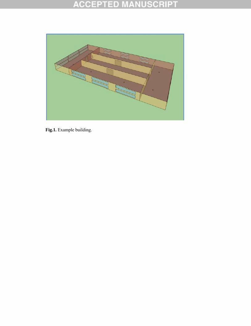
Fig.1. Example building.

Fig.2. Top view of the five-zone layout of the example building.

Fig.3. The number of variables selected into the linear regression models by different criteria for design objectives and constraints.

Table 1 Input variables

VARIABLE INDEX

INPUT VARIABLES UNITS

LOWER BOUND

UPPER BOUND INCREMENT

THE NUMBER

OF VALUE

OPTIONS

1 Heating setpoint (oC) 18.0 22.0 0.5 9

2 Heating set-

back (oC) 0.0 8.0 0.5 17

3 Dead band (oC) 1.0 5.0 0.5 9

4 Orientation (o) -90.0 90.0 5.0 37

5

Façade-1 window-wall

ratio (-) 0.2 0.9 0.1 8

6


ratio (-) 0.2 0.9 0.1 8

7


ratio (-) 0.2 0.9 0.1 8

8


ratio (-) 0.2 0.9 0.1 8

9 Winter start

time (hrs) 1 8 1 8

10 Winter stop

time (hrs) 17 23 1 7

11 Summer start

time (hrs) 1 8 1 8

12 Summer stop

time (hrs) 17 23 1 7

13 External wall

type (-) 0 2 1 3

14 Internal wall

type (-) 0 1 1 2

15 Ceiling-floor

type (-) 0 2 1 3 16 Window type (-) 0 1 1 2

Table 2 Percentage changes in the sensitivity of energy demand to the variables, due

to different selection criteria (AIC and BIC).

Variable

Index

Percentage Changes in Variables Entry-Orders Rank Transformed Data Raw Data

RandomSampleA

RandomSampleB

NSGA-II

RandomSampleA

RandomSampleB

NSGA-II

100 1000

100 1000First100

100 1000 100 1000

First100

1 0 0 0 0 0 0 0 0 0 0 2 0 0 0 0 0 0 0 0 0 3 0 0 0 0 0 0 0 0 0 0 4 0 0 0 0 0 5 0 0 0 0 0 6 0 0 0 0 7 0 0 0 0 0 0 0 0 0 0 8 0 0 0 9 0 0 0 0 0 10 0 11 0 0 0 0 0 0 0 0 0 0 12 0 0 0 0 0 0 0 0 0 13 0 14 0 0 15 0 0 0 0 0 0 0 16 0 0 0 0 0 0 0 0 0

Percentage Changes in Variables SRCs/SRRCs

1 0.065 0.00

0 0.01

8 0.04

7 0.013

0.050

0.000

0.044 0.038

0.004

2 0.150 0.01

6 0.02

0 0.14

0 0.791

0.195

0.000

0.236

0.238

3 0.012 0.00

2 0.00

4 0.00

1 0.053

0.010

0.002

0.051 0.000

0.011

4 0.02

2 0.121

0.045

0.243

0.037

5 0.01

9

0.255

0.04

0

0.523

0.025

6 0.00

0

0.314

0.00

0

0.222

7 0.177 0.00

0 0.03

1 0.06

3 0.171

0.203

0.005

0.041 0.033

8 0.00

0

0.000

0.610

9 0.00

0 0.00

8 0.53

9

0.000

0.192

10 0.123

11 0.149 0.00

6 0.01

4 0.27

7 0.025

0.098

0.005

0.032 0.207

0.077

12 0.093 0.00

0 0.02

1 0.40

2

0.078

0.000

0.111 0.248

0.051

13 0.05

4

14 0.03

3 0.270

15 0.00

0 0.04

1 0.42

6 0.113

0.000

0.053 0.259

16 0.128 0.00

0 0.01

1 0.09

3 0.064

0.121

0.005

0.033 0.006

Percentage Changes in the Size of the R2 Values Attributable to Individual Variables

1 1.52E-06

0 0 0 0 0 0 0 0 0

2 0 0 0 0 0 0 0 0 0

3 5.62E-07

0 0 0 0 0 0 0.047443

0 0

4 0 0 0 0 0 5 0 0 0 0 0 6 0 0 0 0 7 0 0 0 0 0 0 0 0 0 0 8 0 0 0 9 0 0 0 0 0 10 0 11 0 0 0 0 0 0 0 0 0 0 12 0 0 0 0 0 0 0 0 0 13 0 14 0 0 15 0 0 0 0 0 0 0 16 0 0 0 0 0 0 0 0 0

Percentage

changes in

model R2

0.036 0.00

1 0.00

4 0.00

4 0.005

0.025

0.001

0.015 0.001

0.001

Table 3 Percentage changes in the sensitivity of capital costs to the variables, due to

different selection criteria (AIC and BIC).

Variable

Index

Percentage Changes in Variables Entry-Orders

Rank Transformed Data Raw Data RandomSa

mpleA RandomSa

mpleB NSGA-II

RandomSampleA

RandomSampleB

NSGA-II

100 1000 100 1000First100

100 1000 100 1000 First100

1 0 0 0 0 0 0

2 0 0 0

3 0 0 0 0 0 0 0 0 0 0

4 0 0

5 0 0 0 0 0 0 0 0 0 0

6 0 0 0 0 0 0 0 0 0 0

7 0 0 0 0 0 0 0 0 0 0

8 0 0 0 0 0 0 0 0 0 0

9 0 0 0 0 0 0

10 0 0 0 0

11 0 0 0 0 0 0

12 0 0

13 0 0 0 0 0 0 0 0 0 0

14 0 0 0 0 0 0 0 0 0

15 0 0 0 0 0 0 0 0 0 0

16 0 0 0 0 0 0 0 0 0 0

Percentage Changes in Variables SRCs/SRRCs

1 0.00

0 0.04

2

0.684

0.000 0.000 0.65

2

2 0.20

0 0.000

0.133

3 0.00

0 0.00

0 0.00

0 0.27

3 0.000

0.077

0.029 0.09

8 0.05

6 0.113

4 0.000 0.050

5 0.00

0 0.00

6 0.01

5 0.28

0 0.000

0.000

0.007 0.00

6 0.10

7 0.000

6 0.00

0 0.00

7 0.22

0 0.10

2 0.000

0.008

0.000 0.00

8 0.04

7 0.053

7 0.00

0 0.00

7 0.04

4 0.33

6 0.000

0.015

0.000 0.01

5 0.01

5 0.011

8 0.00

0 0.01

1 0.06

3 0.31

9 0.000

0.013

0.000 0.00

0 0.33

7 0.015

9 0.30

8 0.000 0.000

0.091

0.900

0.037

10 0.000 0.000 0.66

7 0.109

11 0.00

0

0.217

0.095

0.042 0.59

1 0.125

12 0.063

0.71

4

13 0.00

0 0.00

0 0.00

0 0.01

1 0.000

0.000

0.000 0.01

3 0.06

9 0.006

14 0.00

0 0.00

0

0.397

0.0000.000

0.000 0.05

3 0.03

5 0.010

15 0.00

0 0.00

1 0.00

1 0.01

3 0.000

0.002

0.000 0.00

0 0.02

2 0.010

16 0.00

0 0.00

0 0.02

1 0.16

1 0.000

0.005

0.000 0.01

0 0.00

5 0.000

Percentage Changes in the Size of the R2 Values Attributable to Individual Variables

1 0 0 0 0 0

2 0 0 0 0

3 0 0 0 0 0 0 0 0 0 0

4 0 0

5 0 0 0 0 0 0 0 0 0 0

6 0 0 0 0 0 0 0 0 0 0

7 0 0 0 0 0 0 0 0 0 0

8 0 0 0 0 0 0 0.215451

0 0 0

9 0 0 0 0 0 0

10 0 0 0 0

11 0 0 0 0 0 0

12 0 0

13 0 0 0 0 0 0 0.177260

0 0 0

14 0 0 0 0 0 0 0 0 0

15 0 0 0 0 0 0 0 0 0 0

16 0 0 0 0 0 0 0 0 0 0 Percen

tage change

s in model

R2

0.000

0.001

0.003

0.000

0.0000.000

0.000 0.00

0 0.00

0 0.000

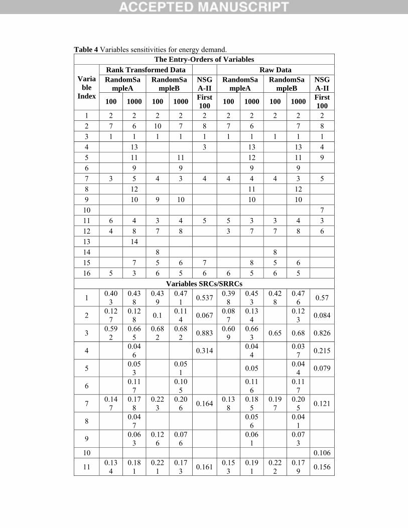
Table 4 Variables sensitivities for energy demand. The Entry-Orders of Variables

Variable

Index


mpleA RandomSa

mpleB NSGA-II

RandomSampleA

RandomSampleB

NSGA-II

100 1000 100 1000 First100

100 1000 100 1000 First100

1 2 2 2 2 2 2 2 2 2 2

2 7 6 10 7 8 7 6 7 8

3 1 1 1 1 1 1 1 1 1 1

4 13 3 13 13 4

5 11 11 12 11 9

6 9 9 9 9

7 3 5 4 3 4 4 4 4 3 5

8 12 11 12

9 10 9 10 10 10

10 7

11 6 4 3 4 5 5 3 3 4 3

12 4 8 7 8 3 7 7 8 6

13 14

14 8 8

15 7 5 6 7 8 5 6

16 5 3 6 5 6 6 5 6 5

Variables SRCs/SRRCs

1 0.40

3 0.43

8 0.43

9 0.47

1 0.537

0.398

0.453

0.428

0.476

0.57

2 0.12

7 0.12

8 0.1

0.114

0.0670.08

7 0.13

4

0.123

0.084

3 0.59

2 0.66

5 0.68

2 0.68

2 0.883

0.609

0.663

0.65 0.68 0.826

4 0.04

6 0.314

0.044

0.03

7 0.215

5 0.05

3

0.051

0.05 0.04

4 0.079

6 0.11

7

0.105

0.11

6

0.117

7 0.14

7 0.17

8 0.22

3 0.20

6 0.164

0.138

0.185

0.197

0.205

0.121

8 0.04

7

0.056

0.04

1

9 0.06

3 0.12

6 0.07

6

0.061

0.07

3

10 0.106

11 0.13

4 0.18

1 0.22

1 0.17

3 0.161

0.153

0.191

0.222

0.179

0.156

12 0.20

5 0.12

2 0.14

0.102

0.20

6 0.12

9 0.16

2 0.11

3 0.175

13 0.03

7

14 0.09

1 0.1

15 0.13

3 0.19

5 0.14

1 0.062

0.125

0.17 0.14

7

16 0.18

7 0.19

1 0.19

0.172

0.1090.14

1 0.18

3 0.18

4 0.16

9

The Size of the R2 Values Attributable to Individual Variables

1 0.1979

0.2023

0.2024

0.2197

0.3158

0.1961

0.2165

0.2082

0.2225

0.3115

2 0.0157

0.0208

0.0081

0.0126

0.0027

0.0073

0.0227

0.0149

0.0066

3 0.5337

0.4308

0.4411

0.4572

0.5009

0.5727

0.4302

0.4703

0.4539

0.5527

4 0.0019

0.058

5

0.0019

0.0013

0.0204

5 0.0024

0.0026

0.0024

0.0019

0.0033

6 0.0117

0.0094

0.0114

0.0116

7 0.0354

0.0342

0.0451

0.0394

0.0416

0.0280

0.0384

0.0362

0.0376

0.0133

8 0.0023

0.0032

0.0015

9 0.0041

0.0117

0.0056

0.0038

0.0053

10 0.008

4

11 0.0125

0.0349

0.0512

0.0294

0.0181

0.0168

0.0402

0.0441

0.0302

0.0291

12 0.0320

0.0148

0.0198

0.0110

0.0386

0.0151

0.0215

0.0130

0.0126

13 0.0013

14 0.0142

0.0095

15 0.0168

0.0285

0.0202

0.0034

0.0164

0.0250

0.0212

16 0.0278

0.0422

0.0287

0.0302

0.0121

0.0172

0.0369

0.0245

0.0282

R2 0.85

5 0.82

0 0.85

1 0.83

7 0.953

0.877

0.839

0.817

0.843

0.958

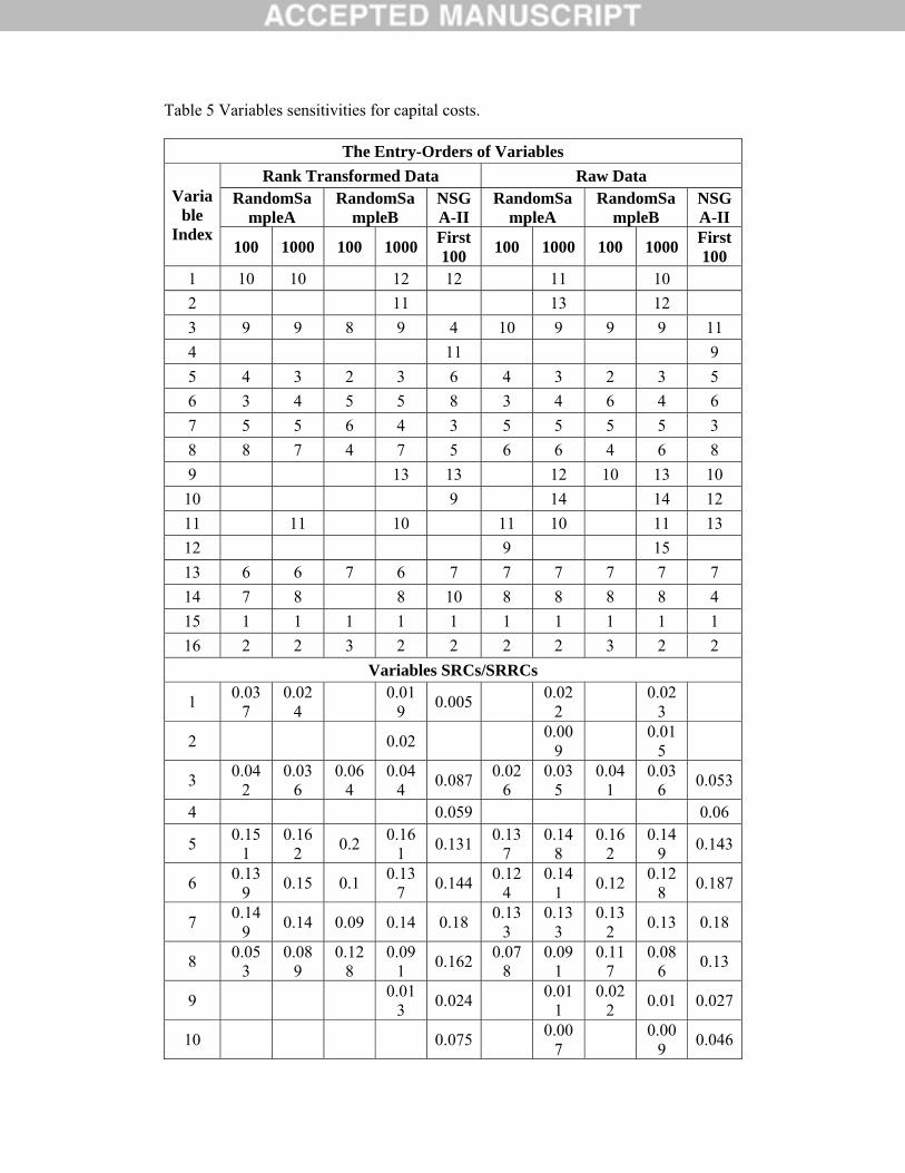
Table 5 Variables sensitivities for capital costs.

The Entry-Orders of Variables

Variable

Index


mpleA RandomSa

mpleB NSGA-II

RandomSampleA

RandomSampleB

NSGA-II

100 1000 100 1000 First100

100 1000 100 1000 First100

1 10 10 12 12 11 10

2 11 13 12

3 9 9 8 9 4 10 9 9 9 11

4 11 9

5 4 3 2 3 6 4 3 2 3 5

6 3 4 5 5 8 3 4 6 4 6

7 5 5 6 4 3 5 5 5 5 3

8 8 7 4 7 5 6 6 4 6 8

9 13 13 12 10 13 10

10 9 14 14 12

11 11 10 11 10 11 13

12 9 15

13 6 6 7 6 7 7 7 7 7 7

14 7 8 8 10 8 8 8 8 4

15 1 1 1 1 1 1 1 1 1 1

16 2 2 3 2 2 2 2 3 2 2


1 0.03

7 0.02

4

0.019

0.005 0.02

2

0.023

2 0.02 0.00

9

0.015

3 0.04

2 0.03

6 0.06

4 0.04

4 0.087

0.026

0.035

0.041

0.036

0.053

4 0.059 0.06

5 0.15

1 0.16

2 0.2

0.161

0.1310.13

7 0.14

8 0.16

2 0.14

9 0.143

6 0.13

9 0.15 0.1

0.137

0.1440.12

4 0.14

1 0.12

0.128

0.187

7 0.14

9 0.14 0.09 0.14 0.18

0.133

0.133

0.132

0.13 0.18

8 0.05

3 0.08

9 0.12

8 0.09

1 0.162

0.078

0.091

0.117

0.086

0.13

9 0.01

3 0.024

0.011

0.022

0.01 0.027

10 0.075 0.00

7

0.009

0.046

11 0.02 0.02

3

0.021

0.024

0.02

2 0.016

12 0.03

2

0.007

13 0.09

2 0.09

3 0.09

4 0.09

5 0.151

0.064

0.082

0.079

0.087

0.159

14 0.06

8 0.06

3

0.063

0.093 0.05 0.05

8 0.05

7 0.05

7 0.104

15 0.88

4 0.91

8 0.93

0.915

1 0.91

9 0.93

6 0.95

6 0.93

5 1.05

16 0.23

3 0.22

4 0.18

7 0.22

4 0.34

0.198

0.209

0.202

0.202

0.309


1 0.0012

0.0006

0.0003

0.0005

0.0005

2 0.0004

0.0007

0.0001

0.0002

3 0.0023

0.0013

0.0040

0.0020

0.0223

0.0007

0.0012

0.0015

0.0013

0.0005

4 0.001

5

0.0023

5 0.0231

0.0258

0.0506

0.0236

0.0103

0.0190

0.0216

0.0371

0.0201

0.0111

6 0.0313

0.0243

0.0104

0.0193

0.0072

0.0282

0.0215

0.0113

0.0163

0.0191

7 0.0176

0.0178

0.0067

0.0187

0.0540

0.0147

0.0160

0.0160

0.0165

0.0383

8 0.0030

0.0085

0.0217

0.0088

0.0129

0.0045

0.0070

0.0170

0.0091

0.0118

9 0.0002

0.0006

0.0001

0.0004

0.0001

0.0007

10 0.002

5

0.0001

0.0001

0.0009

11 0.0004

0.0005

0.0004

0.0006

0.0005

0.0002

12 0.0014

0.0001

13 0.0074

0.0087

0.0079

0.0104

0.0078

0.0039

0.0085

0.0064

0.0077

0.0078

14 0.0034

0.0040

0.0042

0.0027

0.0025

0.0035

0.0033

0.0034

0.0197

15 0.8531

0.8365

0.8359

0.8425

0.7254

0.8860

0.8730

0.8690

0.8786

0.7579

16 0.0401

0.0456

0.0261

0.0471

0.1394

0.0327

0.0397

0.0319

0.0387

0.1266

R2 0.98

3 0.97

3 0.96

3 0.97

8 0.987

0.994

0.993

0.994

0.993

0.997

Table 6 Variables sensitivities for solution infeasibility

The Entry-Orders of Variables

Variable

Index

Rank Transformed Data Raw Data

RandomSampleA

RandomSampleB

NSGA-II

RandomSampleA

RandomSampleB

NSGA-II

100 1000 100 1000 First100

100 1000 100 1000 First100

1 1 1 1 2 1 2 2 2

2

3 2 2 2 1 2 1 1 1

4 5 4

5 5 4 6 1 1

6 6 5 4

7 3 3 3 3 3 4 3

8 3

9 9 6

10 8

11 7 5 7 5 3 4

12 4 8 8 5 7

13

14

15 10 9

16 4 4 2 3 5 2


1 0.69

1 0.62

9 0.66

2 0.65

3

0.563

0.549

0.523

0.553

2

3 0.52

3 0.61

6 0.53

4 0.61

7

0.444

0.55 0.54

3 0.56

8

4 0.3780.15

9

5 0.10

4 0.14

1 0.10

1 0.376 0.42

6 0.09 0.09

6 0.142

7 0.16

5 0.14

6 0.18

3 0.15

1 0.306

0.062

0.09

5

8 0.32

9 0.04

1

0.071

10 0.05

4

11 0.07

4 0.11

0.087

0.15

2 0.08

6

0.085

12 0.08

4 0.05

5

0.044

0.05

7

0.067

13

14

15 0.04

1

0.036

16 0.10

4

0.105

0.2470.15

5

0.074

0.34


1 0.6124

0.3980

0.4784

0.3808

0.3779

0.2972

0.2734

0.2976

2

3 0.2330

0.3801

0.2839

0.4062

0.2133

0.3069

0.2872

0.3118

4 0.074

4 0.0205

5 0.0104

0.0176

0.0097

0.1558

0.080

0

6 0.0089

0.0085

0.0437

7 0.0271

0.0209

0.0397

0.0226

0.0829

0.0039

0.0088

8 0.100

0

9 0.0018

0.0045

10 0.0029

11 0.0061

0.0118

0.0072

0.0218

0.0079

0.0070

12 0.0069

0.0030

0.0019

0.0032

0.0045

13

14

15 0.0016

0.0013

16 0.0118

0.0101

0.0906

0.0318

0.0057

0.0900

R2 0.87

9 0.84

0 0.83

2 0.84

8 0.447

0.665

0.619

0.561

0.643

0.280

Table 7 Categories of variables importance for design objectives and constraints. In

decreasing order of sensitivity, the variables are coloured yellow, green, white, blue.

CATEGORIES OF VARIABLES IMPORTANCE

ENERGY DEMAND CAPITAL COSTS SOLUTION

INFEASIBILITY Heating setpoint Heating setpoint Heating setpoint Heating set-back Heating set-back Heating set-back

Dead band Dead band Dead band Orientation Orientation Orientation

Façade-1 window-wall ratio












Winter start time Winter start time Winter start time Winter stop time Winter stop time Winter stop time

Summer start time Summer start time Summer start time Summer stop time Summer stop time Summer stop time External wall type External wall type External wall type Internal wall type Internal wall type Internal wall type Ceiling-floor type Ceiling-floor type Ceiling-floor type

Window type Window type Window type

a comparison of approaches to stepwise regression on

Documents