Federal Reserve Bank of MinneapolisResearch Department Staff Report 256

Revised September 2000

Paths of Developmentfor Early- and Late-Bloomersin a Dynamic Heckscher-Ohlin Model

Andrew Atkeson∗

University of Minnesotaand Federal Reserve Bank of Minneapolis

Patrick J. Kehoe∗

Federal Reserve Bank of Minneapolisand University of Minnesota

ABSTRACT

We show that in a dynamic Heckscher-Ohlin model the timing of a country’s developmentrelative to the rest of the world affects the path of the country’s development. A country thatbegins the development process later than most of the rest of the world–a late-bloomer–endsup with a permanently lower level of income than the early-blooming countries that developedearlier. This is true even though the late-bloomer has the same preferences, technology, andinitial capital stock that the early-bloomers had when they started the process of development.This result stands in stark contrast to that of the standard one-sector growth model in whichidentical countries converge to a unique steady state, regardless of when they start to develop.

∗Both authors thank the National Science Foundation for research support. Kehoe thanks the Ronald S.Lauder Foundation at the University of Pennsylvania. The views expressed herein are those of the authorsand not necessarily those of the Federal Reserve Bank of Minneapolis or the Federal Reserve System.

The process of development occurs across countries at different times, with some coun-

tries developing relatively early and others developing much later. How does the timing of a

country’s development relative to that of the rest of the world affect the path of the coun-

try’s development? We address this question in a dynamic Heckscher-Ohlin model composed

of a large number of small open economies. Each country has the production structure of

the standard two-sector growth model with consumption and investment goods in which the

two sectors have different capital intensities. These countries differ, however, in the timing

of their development. Some countries, the early-bloomers, reach their steady states before

other countries, the late-bloomers, begin to develop. We find that late-blooming countries

converge to a permanently lower level of output per capita than do early-blooming countries.

This is true even though the late-bloomers have the same preferences, technology, and initial

capital stock that the early-bloomers had when they started to develop. This result stands in

stark contrast to that of the standard one-sector growth model in which identical countries

converge to a unique steady state, regardless of when they start to develop.

The one- and two-sector models give these different results because they imply different

relationships between returns on capital and output. In the one-sector model, equal returns

on capital across countries imply equal output while in the two-sector model, they do not.

More specifically, in the one-sector model, only one capital-labor ratio is consistent with any

given rental rate on capital. This capital-labor ratio uniquely determines a corresponding

level of output. Thus, in the one-sector model, as the rental rates on capital converge across

countries, so do capital-labor ratios and output.

In contrast, in the two-sector model, trade in goods allows for factor price equalization

across countries with different aggregate capital-labor ratios. For countries that diversify

by producing both consumption and investment goods, factor prices are equal. For all such

countries, there is one capital-labor ratio in the consumption good sector and a second ratio in

the investment goods sector. For each of these countries, the country’s aggregate capital-labor

ratio then determines the composition of consumption and investment goods it produces.

Moreover, if capital is added in any such country, output rises, but the rental rate does not

fall. This happens because the country simply produces more of the capital-intensive good.

Thus, in the two-sector model, a whole range of capital-labor ratios is consistent with any

given rental rate, namely, ratios in the cone of diversification. Hence, in the two-sector model,

in the long run, even though rental rates on capital converge, capital-labor ratios and output

do not.

We focus on the path of development for a poor, late-blooming country. We suppose

that this country is sufficiently poor so that it starts the process of development with a capital-

labor ratio lower than that used in the rest of the world to produce the labor-intensive good.

Thus, the late-bloomer starts outside the cone of diversification and specializes in producing

the labor-intensive good. While the late-bloomer is outside this cone, it has a lower capital-

labor ratio than the early-bloomers use in the production of the labor-intensive good and,

hence, a higher rental rate on capital. Thus, the late-bloomer accumulates capital until its

capital-labor ratio equals that used in the rest of the world to produce the labor-intensive

good. At this ratio, the late-bloomer’s rental rate on capital has fallen to the steady-state rate

prevailing in the rest of the world, consumers in the late-blooming country have no further

incentive to accumulate capital, and the country’s growth stops at the lower edge of the cone

of diversification. Thus, the late-bloomer never catches up to the rest of the world.

Our study is related to the literature which considers open economy versions of stan-

2

dard two-sector growth models. For example, Oniki and Uzawa (1965) consider this type of

model with exogenous and constant savings. Oniki and Uzawa find that each country has a

unique steady-state level of capital. Hence, in their model, all countries converge to the same

level of output in the steady state regardless of the timing of development. In our model, in

contrast, the savings rate is not constant, but rather is derived from utility maximization;

our model thus has a continuum of steady states, each of which corresponds to a different

savings rate.

There is also some work on dynamic Heckscher-Ohlin models in which savings is de-

termined from utility maximization. Stiglitz (1970) and Baxter (1992) restrict their attention

to steady states. They study the patterns of trade that arise in a standard two-sector model

when countries have either different fiscal policies or different preferences. Ventura (1997)

uses an alternative formulation of a two-sector model in which there is a single final good

produced by two traded intermediate goods. In it he imagines that the world economy is

composed of countries with different initial conditions that all develop simultaneously. He fo-

cuses on how the model’s predictions for conditional convergence of output per capita across

countries depend on the elasticity of substitution between capital and labor.

All of these studies, including ours, build on the large literature on closed economy two-

sector growth models. (See Uzawa 1964 for an early treatment and Benhabib and Nishimura

1983 for a more recent treatment.)

Our main result has some of the same flavor as results in the endogenous growth

literature, including those of Krugman (1987), Boldrin and Scheinkman (1988), Lucas (1988),

Stokey (1991), Young (1991), and Matsuyama (1992). In some of this work, poor countries

have an initial static comparative advantage in industries with limited learning opportunities.

3

Hence, poor countries tend to specialize in such industries and have permanently lower growth

rates than the rest of the world. In our model, in the long run, all countries have the same

rate of growth but different levels of output.

1. The Economy

Consider a world economy consisting of a large number of small countries that differ

only in their timing of development. The preferences of consumers in each country are given

by

Z ∞

0e−ρtu (ct) dt.(1)

In each country, the constant returns to scale production functions for consumption c and

investment x goods are Fi (Ki, Li), which in intensive form are fi (ki) li, where ki = Ki/Li

and li = Li/L for i = c, x. Let k denote the ratio of the total capital stock K to total labor L

in a given country. Assume that f0i > 0, f

00i < 0, f

0i (0) =∞, and f 0i (∞) = 0 and that there

are no factor intensity reversals. Assume that investment goods are more capital-intensive

than consumption goods, so that kx > kc for any wage-rental ratio. The constraints on labor

and capital within a country are

lc + lx = 1(2)

kclc + kxlx = k.(3)

Capital accumulation within a country is governed by

k = x− δk(4)

where x is investment and δ is the depreciation rate.

4

Consumers in each country trade consumption and investment goods, taking as given

the time path for p, the world price of the investment good relative to the consumption good.

Assume that trade for each country is balanced at each date, so that c + px = rk + w,

where r is the rental rate on capital and w is the wage rate in that country. Accordingly, the

representative consumer in each country chooses time paths for consumption and capital to

maximize (1) subject to

k = (rk + w − c) /p− δk(5)

with k ≥ 0. Firms in each country maximize

fc(kc)lc + pfx(kx)lx − r(kclc + kxlx)− w(lc + lx).(6)

We will use repeatedly the following first-order conditions derived from the consumers’

and firms’ problems. The first-order conditions characterizing the solution to each consumer’s

problem are found from the Hamiltonian

H = e−ρt{u (c) + q([rk + w − c]/p− δk)}

where q is the co-state variable. The optimality conditions include the static first-order

condition

u0(c) = q/p(7)

and the canonical equation

q

q= ρ+ δ − r/p.(8)

The static first-order conditions describing production efficiency are given by

f 0c(kc) = pf0x(kx) = r(9)

5

fc(kc)− f 0c(kc)kc ≤ w(10)

pfx(kx)− pf 0x(kx)kx ≤ w(11)

where (10) holds with equality if lc > 0 and (11) holds with equality if lx > 0.

2. Early- vs. Late-Bloomers

In comparing the development of early- and late-bloomers, we first solve for the steady-

state output and prices for early-bloomers. We then use these steady-state prices as the world

prices faced by a late-blooming country.

A. Early-Bloomers

Consider first the steady state for the early-bloomers. Imagine, for simplicity, that

all but one of the countries start developing at the same time with the same initial capital

stocks. Assume that the late-bloomer is a small country, so its behavior does not affect the

time path for the world price p.

Clearly, in equilibrium, all the identical early-blooming countries make the same

choices; hence, the equilibrium for this world economy is the same as one for a single large

country that does not trade. Using this equivalence, write the world resource constraints as

c = fc(kc)lc(12)

x = fx(kx)lx.(13)

In equilibrium, consumers maximize utility, firms maximize profits, and (2)—(3) and (12)—(13)

hold.

6

Denote the steady-state prices and quantities for the early-bloomers by p, r, w, and k,

and denote their steady-state techniques of production by kx and kc. Note that in a steady

state, the world will clearly produce some consumption goods. It will also produce investment

goods to replace depreciated capital. Thus,

kc < k < kx(14)

and (10) and (11) hold with equality. These steady-state prices and quantities are found as

the solutions to (2)—(4), (7)—(9), (10)—(11), and (12)—(13), with p = k = q = 0. Notice that

in a steady state, (8) implies that

r = p(ρ+ δ).(15)

B. The Late-Bloomer

Consider next the path of development for the small country starting the process of

development late. In particular, assume that the rest of the countries in the world have

already reached their steady state before this small country removes the domestic distortions

that have kept its capital stock relatively low and, hence, kept the country poor.

The path of development of the late-bloomer depends on the late-bloomer’s capital-

labor ratio relative to the ratios in the cone of diversification. This cone is defined as the

set of capital and labor endowments for which the late-bloomer produces both consumption

and investment goods. The cone consists of the pairs of capital and labor (K,L) such that

the ratio k = K/L is in the interval [kc, kx]. When the late-bloomer’s capital and labor lie in

this cone, the late-bloomer’s factor prices are equal to those of the early-bloomers.

We solve for the path of development for this late-blooming country taking as given

the world price p as follows. Since p = 0, from (7) we have that q/q = −σ(c)c/c, where

7

σ(c) = −u00 (c) c/u0 (c) . Thus, our dynamical system is

c

c=

1

σ(c)

"r

p− (ρ+ δ)

#(16)

and (5) with p = p, and r and w are determined as functions of k in three regions: k ∈³0, kc

´;

k ∈hkc, kx

i; and k ∈

³kx,∞

´.

When k ∈³0, kc

´, the late-bloomer’s capital-labor ratio is below the cone of diversi-

fication. Comparative advantage requires that the late-bloomer specialize in the production

of consumption goods since these are labor-intensive. Thus, (9) and (10) imply that the late-

bloomer’s factor prices are given by r = f 0c (k) and w = fc (k)−f 0c (k) k. Hence, the dynamical

system (16) and (5) in this region reduces to

c

c=

1

σ(c)

"f 0c (k)p

− (ρ+ δ)#

(17)

k =1

p[fc (k)− c]− δk.(18)

When k ∈hkc, kx

i, the late-bloomer has a capital-labor ratio in the cone of diversifi-

cation, it produces some of each good, and its factor prices are equal to those in the rest of

the world. Since r = r and w = w in this region, the dynamical system (16) and (5) reduces

to

c = 0

k =1

p[rk + w − c]− δk

where the first equation follows from (15).

Finally, when k ∈³kx,∞

´, the late-bloomer’s capital-labor ratio is above the cone of

diversification. Comparative advantage requires that the late-bloomer specialize in the pro-

duction of the investment good since that good is capital-intensive. Thus, (9) and (11) imply

8

that the late-bloomer’s factor prices are given by r = pf 0x (k) and w = p (fx (k)− f 0x (k) k),

and the dynamical system (16) and (5) in this region reduces to

c

c=

1

σ(c)[f 0x (k)− (ρ+ δ)]

k = fx (k)− δk − c/p.

These dynamics for the late-bloomer are summarized in the phase diagram in Figure

1. In terms of the dynamics of consumption, notice that c > 0 when k < kc since f 0c(k) > r,

that c = 0 when kc ≤ k ≤ kx, and that c < 0 when k > kx since pf 0x (k) < r. In terms of the

dynamics of capital, the k = 0 locus is defined by three segments: for k < kc, this locus is

defined by c = fc(k)− pδk, which is increasing and concave; for kc ≤ k ≤ kx, it is defined by

c = (r − pδ)k + w, which is a straight line with a positive slope; and for k > kx, it is defined

by c = p(fx(k) − δk), which is increasing and concave up to k∗x, defined by f 0x(k∗x) = δ, and

decreasing thereafter.

In terms of the dynamic path, notice that for all k0 < kc, consumption c0 jumps to

the corresponding point on the unique path (labeled D0D) that converges to the point D

on the lower boundary of the cone of diversification. Along this path, wages are rising and

rental rates are falling. In the region where k0 < kc, the rental rate is higher than that in

the rest of the world, so the late-bloomer accumulates capital and increases consumption.

For kc ≤ k0 ≤ kx, consumption c0 jumps to the corresponding point on the k = 0 locus

(labeled E), and consumption and the capital stock stay fixed. In this region, rental rates

are equal to those in the rest of the world, and the level of c adjusts so that the late-bloomer

keeps the capital stock and consumption fixed. For k0 > kx, consumption c0 jumps to the

corresponding point on the unique path (labeled F0F ) that converges to the point F on the

9

upper boundary of the cone of diversification. In the region where k0 > kx, the rental rate

on capital is lower than in the rest of the world, so the late-bloomer decumulates capital and

reduces consumption.

C. A Comparison

Trade patterns in the steady state depend on the relationship between the late-

bloomer’s and the early-bloomers’ capital-labor ratios, k and k. If the late-bloomer reaches

its steady state with k < k, it exports consumption goods and imports investment goods. If

it reaches its steady state with k > k, it exports investment goods and imports consumption

goods. The volume of trade increases with the distance of k from k.

Notice from Figure 1 that if the late-blooming country starts the process of develop-

ment with some k0 ∈ (0, kc), then over time the country’s capital-labor ratio converges to the

point kc at the edge of the steady-state cone of diversification. This capital stock kc is strictly

less than the capital-labor ratio k for the early-bloomers. In the steady state for the late-

bloomer, its steady-state factor prices r and w are equal to those in the rest of the world (r

and w) since its capital stock kc is in the cone of diversification for the world economy. Thus,

steady-state output for the late-bloomer (rkc + w) is lower than that for the early-bloomers

(rk + w).

Summarizing these results, we have this proposition:

Proposition. A late-bloomer never catches up with the early-bloomers, in the sense that the

steady-state output for a late-bloomer with k0 < kc is lower than that of early-bloomers with

the same initial capital stock.

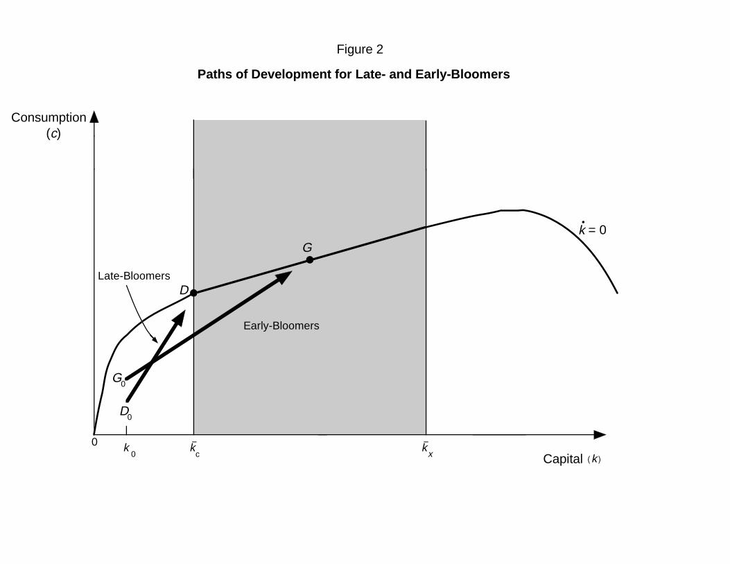
In a separate appendix (Atkeson and Kehoe 1998), we consider an economy with a

10

constant relative risk aversion utility function U(c) = c1−σ/(1 − σ) and a Cobb-Douglas

production function fi(k) = kαi, where i = c, x with αc < αx. We show that locally late-

bloomers converge to their steady state faster than do early-bloomers. We show that the same

result holds globally for numerical examples. In Figure 2 we plot the paths of development

for an early-bloomer and a late-bloomer that begin with the same capital stock.

One way to get some intuition for this result is to recall that in a one-sector model

the speed of convergence is slower the larger is the capital share (King and Rebelo 1993).

The late-bloomers specialize in the labor-intensive good, consumption; and the eigenvalue

governing their speed of convergence is identical to that in a one-sector growth model. The

early-bloomers produce both goods, and the eigenvalue governing their speed of convergence

is determined by a weighted-average of the capital shares in both sectors. Since the late-

bloomers specialize in the good with the lower capital share, their speed of convergence is

faster.

So far we have assumed that trade is balanced at each date. If we allow borrowing and

lending, then neither the steady state nor the dynamics of the early-bloomers changes since

there is no incentive to borrow or lend among identical countries. For the late-bloomers, the

steady state does not change, but the dynamics does change, significantly. A late-bloomer

with a very low capital stock borrows enough so that its capital instantly jumps to the

lower edge of the cone of diversification. This country’s GDP is the same as that in the

model without borrowing or lending, but its GNP is lower by the interest payments on the

accumulated debt.

11

3. An Alternative Formulation

Here we consider a two-sector model in which there is a single final good that is made

from two intermediate goods (as in Backus, Kehoe, and Kydland 1994 and Ventura 1997).

We use this formulation to show that our main result does not require that consumption and

investment goods differ in their factor intensities.

Let the production technology for final goods be given by

c+ x = G(a, b)

where G is constant returns to scale and a and b are intermediate goods. We assume that

G is strictly concave, is twice differentiable, and satisfies the Inada conditions Ga(0, b) =∞

and Gb(a, 0) = ∞. Intermediate goods a and b are produced using capital and labor with

constant returns to scale production functions of the form

ya = Fa(Ka, La) = fa(ka)la

yb = Fb(Kb, Lb) = fb(kb)lb.

We assume that f 0i > 0, f00i < 0, f

0i(0) =∞, and f 0i(∞) = 0. Assume that intermediate good

b is capital-intensive relative to good a in the sense that kb > ka for any factor prices w/r.

The constraints for capital and labor within a country are

la + lb = 1(19)

kala + kblb = k.(20)

Capital accumulation is governed by

k = x− δk.

12

Each country is small relative to the world economy, and all world prices are taken as

given. Each country trades only intermediate goods, and trade is balanced so that

paa+ pbb = paya + pbyb

where pi is the relative price of intermediate good i in terms of the final good (whose price is

normalized to one). Note that the income of the country is also given by rk+w, so balanced

trade also requires that c+ x = rk + w.

Consumers solve

maxZ ∞

0e−ρtu (ct) dt

k = [rk + w − c]− δk.(21)

Final goods firms solve

maxa,b

G(a, b)− paa− pbb.

Intermediate goods firms for goods a and b solve

maxka,la

pafa(ka)la − rkala − wla

maxkb,lb

pbfb(kb)lb − rkblb − wlb.

The Hamiltonian associated with the consumer’s problem is

H = e−ρt{u (c) + q([rk + w − c]− δk)}

which has the static first-order condition

u0(c) = q

13

and the canonical equation

q

q= σ(c)

c

c= [(ρ+ δ)− r] .(22)

Intermediate goods firms’ first-order conditions include

paf0a(ka) = pbf

0b(kb) = r(23)

pafa(ka)− paf 0a(ka)ka ≤ w(24)

pbfb(kb)− pbf 0b(kb)kb ≤ w(25)

where (24) and (25) hold with equality if la > 0 and lb > 0, respectively.

As before we assume that there are a large number of identical early-bloomers and one

small late-bloomer whose behavior does not affect world prices. The equilibrium for the world

economy is the same as one for a single large closed economy with resource constraints (19),

(20), and a = fa(ka)la, b = fb(kb)lb. The steady state for the early-bloomers is a solution to

the first-order conditions of the consumer and the firms with c = k = 0, together with these

resource constraints. Given our assumptions on the technologies, there is a unique steady

state and both goods a and b are produced in the world at all times. Let pa, pb, r, w, ka, kb, k

with ka < k < kb denote the steady-state prices and quantities for the early-bloomers. In the

steady state, r = ρ+ δ.

The dynamical system for late-bloomers, taking prices pa and pb as given, is

c

c=

1

σ(c)[r − (ρ+ δ)]

and (21) with factor prices determined as functions of k in three regions: k ∈ (0, ka); k ∈hka, kb

i; and k ∈ (kb,∞). When k < ka, the late-bloomer specializes in the labor-intensive

14

good a, and thus (23) and (24) imply that r = paf 0a(k) and w = pa(fa(k)− f 0a(k)k). Hence,

the dynamical system reduces to

c

c=

1

σ(c)[f 0a(k)− (ρ+ δ)]

k = fa(k)− c− δk.

When ka ≤ k ≤ kb, the late-bloomer has a capital-labor ratio in the cone of diversification

and its factor prices are equal to those in the rest of the world. Since r = r and w = w in

this region, the dynamical system reduces to

c = 0

k = rk + w − c− δk.

When k > kb, the late-bloomer specializes in the capital-intensive good b, and thus (23) and

(25) imply that r = pbf 0b(k) and w = pb(fb(k)−f 0b(k)k). Hence, the dynamical system reduces

to

c

c=

1

σ(c)[f 0b(k)− (ρ+ δ)]

k = fb(k)− c− δk.

The phase diagram summarizing these dynamics is identical to Figure 1. Thus, the

analog of our Proposition holds for this economy.

4. Summary

We have shown that in a standard two-sector model with trade, the timing of develop-

ment affects the paths of development. We have found that late-blooming countries converge

15

permanently to a lower level of output per capita than do early-blooming countries. We have

shown that this is true even though late-bloomers have the same preferences, technology, and

initial capital stock that the early-bloomers had when they started on the path to develop-

ment. These results are strikingly different from those of the standard one-sector growth

model.

16

References

Atkeson, Andrew, and Kehoe, Patrick J. 1998. Appendix to “Paths of development for

early- and late-bloomers.” Manuscript. Research Department, Federal Reserve Bank

of Minneapolis.

Backus, David K.; Kehoe, Patrick J.; and Kydland, Finn E. 1994. Dynamics of the trade

balance and the terms of trade: The J-curve? American Economic Review 84: 84—103.

Baxter, Marianne. 1992. Fiscal policy, specialization, and trade in the two-sector model:

The return of Ricardo? Journal of Political Economy 100 (August): 713—44.

Benhabib, Jess, and Nishimura, Kazuo. 1983. The paths of optimal economic development.

Keio Economic Studies 20 (1): 1—22.

Boldrin, Michele, and Scheinkman, Jose A. 1988. Learning-by-doing, international trade and

growth: A note. In The economy as an evolving complex system: The proceedings of

the Evolutionary Paths of the Global Economy Workshop, ed. Philip W. Anderson,

Kenneth J. Arrow, David Pines, pp. 285—300. Santa Fe Institute Studies in the

Sciences of Complexity, Vol. 5. Redwood City, Calif.: Addison-Wesley.

King, Robert G., and Rebelo, Sergio T. 1993. Transitional dynamics and economic growth

in the neoclassical model. American Economic Review 83 (September): 908—31.

Krugman, Paul. 1987. The narrow moving band, the Dutch disease, and the competitive

consequences of Mrs. Thatcher. Journal of Development Economics 27 (October):

41—55.

Lucas, Robert E., Jr. 1988. On the mechanics of economic development. Journal of Monetary

Economics 22 (July): 3—42.

17

Matsuyama, Kiminori. 1992. Agricultural productivity, comparative advantage, and eco-

nomic growth. Journal of Economic Theory 58 (December): 317—34.

Oniki, Hajime, and Uzawa, Hirofumi. 1965. Patterns of trade and investment in a dynamic

model of international trade. Review of Economic Studies 32 (January): 15—38.

Stiglitz, Joseph E. 1970. Factor price equalization in a dynamic economy. Journal of Political

Economy 78 (May—June): 456—88.

Stokey, Nancy L. 1991. Human capital, product quality, and growth. Quarterly Journal of

Economics 106 (May): 587—616.

Uzawa, Hirofumi. 1964. Optimal growth in a two-sector model of capital accumulation.

Review of Economic Studies 34 (January): 1—24.

Ventura, Jaume. 1997. Growth and interdependence. Quarterly Journal of Economics 112

(February): 57—84.

Young, Alwyn. 1991. Learning by doing and the dynamic effects of international trade.

Quarterly Journal of Economics 106 (May): 369—405.

18

D

Figure 1

D

E

k k k(k)

(c)

k = 0

Phase Diagram for Late-Bloomers

F

D k E k

F

c = 0c > 0 c < 0

0 c 0 x 0

0

0

Consumption

0

Capital

�

F− −

��

�

�

�

�

D

Figure 2

D

G

k k k( k)

(c)

k = 0

Paths of Development for Late- and Early-Bloomers

0 c x

0

Consumption

0

Capital

.

− −

G0

Early-Bloomers

Late-Bloomers

�

�

�