J. Duncan and G. Gerig (Eds.): MICCAI 2005, LNCS 3750, pp. 41 – 48, 2005. © Springer-Verlag Berlin Heidelberg 2005

Passive Markers for Ultrasound Tracking of Surgical Instruments

Jeffrey Stoll and Pierre Dupont

Boston University, Aerospace and Mechanical Engineering Department, Boston, MA

{jstoll, pierre}@bu.edu

Abstract. A family of passive markers is presented by which the position and orientation of a surgical instrument can be computed from its ultrasound image using simple image processing. These markers address the problem of imaging instruments and tissue simultaneously in ultrasound-guided interventions. Marker-based estimates of instrument location can be used in augmented reality displays or for image-based servoing. Marker design, measurement techniques and error analysis are presented. Experimentally determined in-vitro measurement errors of 0.22 mm in position and 0.089 rad in orientation were obtained using a standard ultrasound imaging system.

1 Introduction

While ultrasound imaging has traditionally been employed for diagnostic procedures, its use in minimally invasive interventions is growing. The advent of real-time 3D ultrasound is also likely to facilitate these procedures. For example, in cardiac surgery, ultrasound imaging can be used for beating-heart repair of internal defects [ 1].

A challenge arises, however, due to the substantial difference in both impedance and absorption of biological tissues and instruments. Imaging systems designed to differentiate tissue types based on small changes in impedance are not well suited to imaging metal instruments. As a result, instruments produce image artifacts due to specular reflection and scattering, which obscure both the location and geometric details of the instrument. The instrument markers presented here address this problem by providing a means to easily estimate an instrument’s body coordinate frame from a single ultrasound image. Such estimates can be used to augment ultrasound images with precise instrument location or to register instruments with respect to a manipulating robot for image-based servoing.

Alternate solutions to the instrument imaging problem include instrument modification, image processing techniques and the use of active markers. In instrument modification, several researchers have focused on altering instruments’ reflection characteristics to make them more visible [ 2]. This approach can involve the application of coatings or surface modifications to the instruments, which can add cost while not necessarily eliminating image artifacts. Image processing methods apply search techniques based on either actual instrument geometry or the geometry produced under ultrasound imaging [ 3]. This approach shows promise although the amount of processing involved may be tied to the complexity of the geometry. Other

42 J. Stoll and P. Dupont

work has focused on actively tracking instruments and ultrasound transducers using electromagnetic and optical sensors. Lindseth et al. report measurement accuracy of 0.6 mm with optical tracking of the ultrasound scan head [ 4], and Leotta reported accuracy of 0.35 mm with electromagnetic tracking [ 5]. Merdes and Wolf reported a method for tracking an active ultrasound receiver mounted on a cardiac catheter [ 6]. They achieved a mean accuracy between 0.22±0.11 and 0.47±0.47 mm, depending on the distance between the catheter and the ultrasound transducer. Active tracking devices are more costly than passive ones. They also can require more complex calibration and can be more difficult to integrate with existing medical instruments.

The solution presented here consists of passive markers which can be easily added to existing surgical instruments and require minimal calibration. The markers are constructed to possess two properties: (1) they appear clearly when imaged along with tissue regardless of instrument appearance, and (2) they are shaped such that their positions and orientations can be determined from a single image using simple image processing.

In this paper, we assume that the instruments possess a cylindrical shaft over which the marker can be attached as shown in Figure 1. The cylindrical portion of the marker is used to determine the four degrees of freedom associated with the instrument shaft axis. The marker pattern is designed to indicate the location of the marker along the instrument shaft and the rotation of the marker about the shaft’s axis. The proposed markers are applicable to both 2D and 3D ultrasound. For simplicity of presentation, only the 2D case is considered here.

These markers are similar to devices known as stereotactic frames, which have been studied extensively for imaging modalities such as CT and MRI [ 7][ 8]. A stereotactic frame consists of a shape that appears uniquely when imaged at various positions and orientations and is constructed of material easily seen in a particular imaging modality.

The next section describes the proposed family of markers – their design, image processing and error analysis. The subsequent section presents an experimental evaluation of one possible marker shape and the paper concludes with a discussion of the results.

2 Implementation

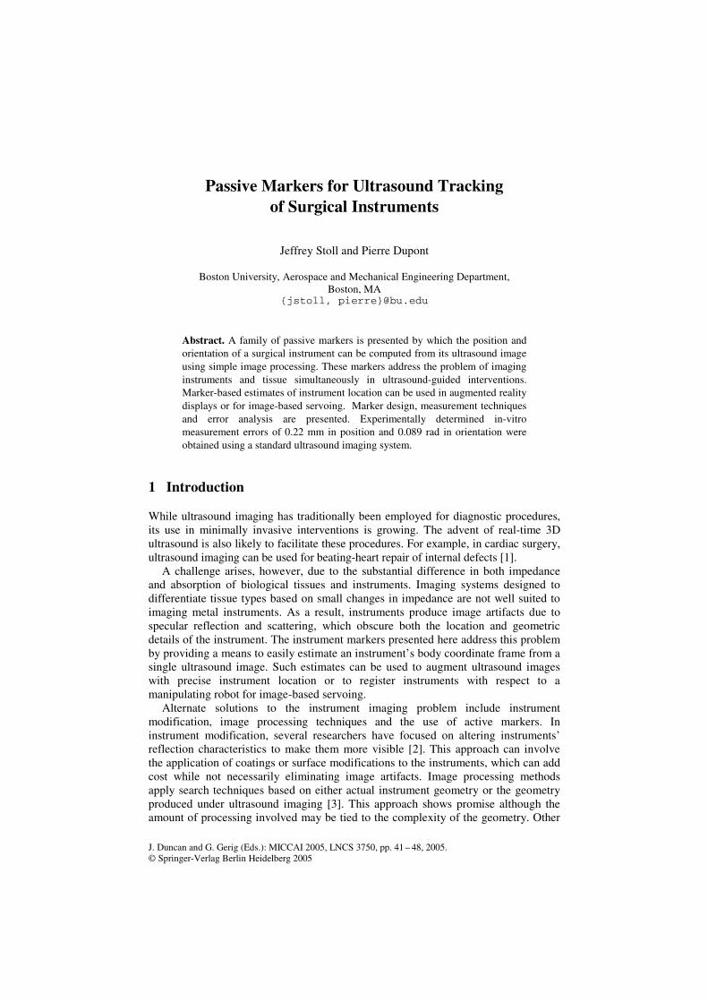
The markers consist of two parts, a cylindrical sleeve that can be fit over the shaft of a surgical instrument and ridges of constant height and width fixed to the outer surface of the sleeve, as shown in Figure 1. The cylindrical shape allows the markers to fit

(a)

(b)

Fig. 1. Two possible marker designs attached to a surgical grasping instrument

Passive Markers for Ultrasound Tracking of Surgical Instruments 43

through access ports used in minimally invasive surgery. The ridges trace out prescribed paths on the sleeve’s surface, which, when imaged, indicate the marker’s position along and orientation about the cylinder’s axis. The family of markers is characterized by a variable number of ridges and a variety of ridge paths. These are together referred to as the marker pattern.

The marker pattern must satisfy three constraints. First, each position along and rotation about the cylinder’s axis must correspond to a unique ultrasound image of marker pattern. Second, the error in position and orientation should be small. Third, the length of the marker pattern should be small since ultrasound imaging systems typically have a small field of view. Note that the marker body can extend beyond the marker pattern in order to make the instrument shaft visible.

2.1 Marker Analysis

If the relative position and orientation of the instrument and marker are known, the rigid body transformation, M

IT , relating the marker coordinate frame to the image-

based coordinate frame defines the instrument’s position and orientation relative to the ultrasound image. This transformation can be decomposed into two elements,

.M A MI I AT T T= (1)

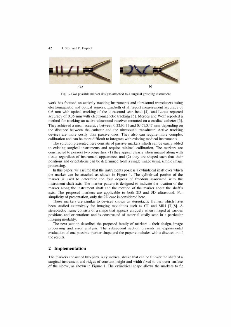
As shown in Figure 2, transformation AIT relates an intermediate frame,A , located

on the instrument shaft’s axis, with the image frame. This frame, determined in an initial processing step, serves to locate the axis of the instrument shaft in the image. The second transformation, ( , )M

AT tθ , defines the marker frame with respect to the

shaft axis frame in terms of θ and t , the rotation about, and the translation along, the shaft axis Ax . The entire length of the marker body can be used to estimate the shaft

axis frame while the marker pattern is used to estimate θ and t . Assuming the instrument shaft lies in the plane of the 2D ultrasound image, the

marker body appears as a line of high pixel intensity. This line represents a thin strip along the surface of the marker facing the ultrasound transducer. The marker pattern appears as a sequence of bumps along the bright line produced by the body.

ultrasound image

instrument

x’

θ

image coordinate frame

ultrasound image

instrument

t

θ

image coordinate frame

marker coordinate frame

intermediateframe

MxMy

Mz Ax AyAz

IxIy

Iz

IArultrasound image

instrument

x’

θ

image coordinate frame

ultrasound image

instrument

t

θ

image coordinate frame

marker coordinate frame

intermediateframe

MxMy

Mz Ax AyAz

IxIy

Iz

IAr

Fig. 2. Ultrasound image plane and coordinate systems Fig. 3. Marker pattern

44 J. Stoll and P. Dupont

The transformation AIT is estimated by fitting a line to the high intensity marker

body image and selecting as the frame’s origin, IAr , one of the two points where this

line intersects the image boundary. The frame’s x-axis, Ax is selected to lie along the

instrument’s shaft axis and its z-axis, Az is taken to coincide with Iz , orthogonal to

the image plane. Note that the axis Ax is offset from the image line in the Ay±

direction by the known radius of the marker body. Transformation M

AT is estimated from the bump locations associated with the

imaged marker pattern. As shown in Figure 3, the Ax coordinates of the n bumps are

combined in a vector [ ]1 2, , ,T

nl l l l= … . This vector is related to the marker pattern

through θ and t by

( )( )

( )

( )( )

( )

1 1

2 2

, 1

, 1,

, 1n n

l t f

l t ftu u

l t f

M M M

θ θθ θ

θ θ

⎡ ⎤ ⎡ ⎤ ⎡ ⎤⎢ ⎥ ⎢ ⎥ ⎢ ⎥⎢ ⎥ ⎢ ⎥ ⎢ ⎥⎢ ⎥ ⎢ ⎥ ⎢ ⎥= + =⎢ ⎥ ⎢ ⎥ ⎢ ⎥⎢ ⎥ ⎢ ⎥ ⎢ ⎥⎢ ⎥ ⎢ ⎥ ⎢ ⎥⎢ ⎥⎢ ⎥ ⎢ ⎥ ⎣ ⎦⎣ ⎦ ⎣ ⎦

, (2)

in which the components of the vector ( )f θ are functions describing the Mx

coordinates of the marker ridges as functions of rotation angle θ about Mx . In this

equation, t is seen to be the magnitude of AMr , the vector describing the origin of

marker frame M with respect to shaft axis frame A , measured along Ax .

In terms of the vector l , the constraint that each position along, and rotation about, the cylinder’s axis corresponds to a unique ultrasound image of marker pattern can be expressed as

( ) ( ) ( ) ( )1 1 2 2 1 1 2 2, , 0 , , [0 2 ),l t l t t t tθ θ θ θ θ π− = ⇔ = ∀ ∈ … ∈ℜ . (3)

Combining (2) and (3) gives the constraint in terms of ( )f θ ,

( ) ( )1 2f f au aθ θ− ≠ ∀ ∈ℜ . (4)

By (2), a marker pattern must possess at least two ridges ( 2n ≥ ) to provide a unique solution for θ and t . By (4), the curves describing these two ridges must differ. For markers with more than two ridges, (2) is overdetermined providing the means to reduce measurement error. For marker patterns satisfying (4), solutions for θ and t can be found by the following procedure. First note that t can be expressed explicitly in terms of θ by

( )( ) /Tt u l f nθ= − . (5)

The error vector ( )l f tuθ− − can be expressed solely in terms of θ using (5) and its

minimum norm solution corresponds to θ ,

( )( )

0 2arg min ( )

Tu l fl f u

nα π

αθ α

≤ <

−= − − . (6)

Passive Markers for Ultrasound Tracking of Surgical Instruments 45

2.2 Error Analysis

The resolution of the marker depends fundamentally on the error in measuring the individual components of l . This error arises from four sources: random noise, finite image resolution, marker manufacturing defects, and misalignment between the image plane and instrument shaft. Since noise and image resolution involve the imaging system, they are assumed to affect all elements of l equally and are treated as one error source. While manufacturing defects can cause unevenly distributed error, for simplicity they are treated here as noise affecting all elements equally. Distortion of l caused by misalignment of the instrument in the image plane is assumed to be small, due to both the length of the instrument shaft and the narrow width of the ultrasound image.

Error estimates in t and θ based on measuring the components of l can be obtained by first linearizing (2) about a nominal angle, 0θ .

( )0 0

0 0 0 0( ) ( )f f

l tu f f utθ θ

θθ θ θ θ γ θ

θ θ

⎛ ⎞ ⎡ ⎤⎛ ⎞ ⎛ ⎞∂ ∂ ⎟⎜⎟ ⎟⎜ ⎜ ⎟ ⎡ ⎤ ⎢ ⎥′⎜= + + − = +⎟ ⎟ ⎟⎜ ⎜⎜ ⎣ ⎦⎟ ⎟⎟ ⎟ ⎟⎜ ⎜ ⎢ ⎥⎜⎝ ⎠ ⎝ ⎠ ⎟∂ ∂⎜ ⎟⎝ ⎠ ⎣ ⎦. (7)

Least squares solutions for t and θ are given by the pseudoinverse of 0( )f uθ⎡ ⎤′⎣ ⎦ as

( ),T T

T T

b f ut l b u f

b u f fγ

⎛ ⎞⎛ ⎞′ ⎟⎜ ⎟⎜ ⎟′⎟⎜= − = −⎜ ⎟⎟⎜ ⎜ ⎟⎟⎜ ⎟ ⎟′ ′⎜⎜ ⎝ ⎠⎝ ⎠ (8)

( ),T T

T T

c f ul c f u

c f u uθ γ

⎛ ⎞⎛ ⎞′ ⎟⎜ ⎟⎜ ⎟′ ⎟⎜= − = −⎜ ⎟⎟⎜ ⎜ ⎟⎟⎜ ⎟ ⎟′ ⎜⎜ ⎝ ⎠⎝ ⎠ (9)

The linearized error estimate for t and θ is given by multiplying the error factors Tb b u and Tc c f ′ , respectively, by the standard deviation of the error in the

components of l . The error factors are functions of the nominal angle 0θ .

Marker pattern length corresponds to the total range of values in ( )f θ . As can be

seen in (8) and (9), design changes, such as increasing the number of ridges (ie. increasing u ) or increasing the ridge slope, ′f , can reduce the error factors. Such changes, however, also increase the marker pattern length. As a result, there exists a tradeoff in marker design between the stated design constraints of minimizing measurement error and minimizing pattern length.

3 Example

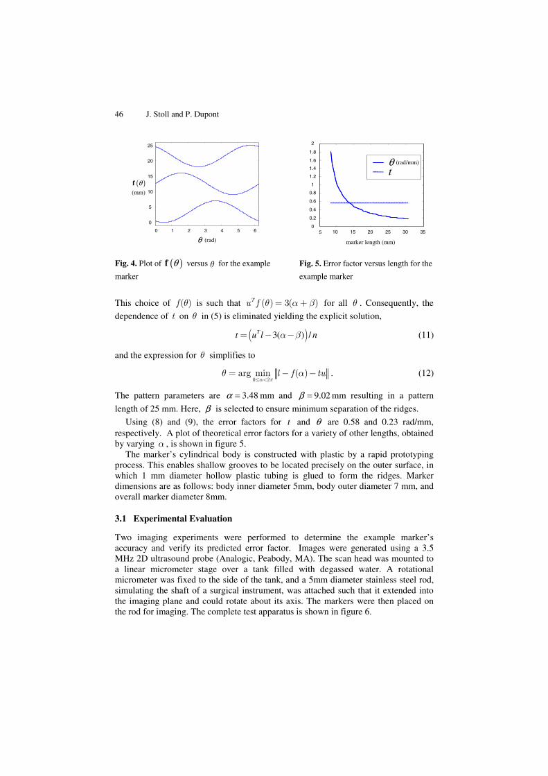
Figure 4 depicts one possible marker pattern (also shown in Figures 1b and 3) consisting of three ridges described by sine waves of equal amplitude, but with phase lags of 2 /3π and displacement offsets of β ,

( ) ( ) 2 4sin , sin , sin 2

3 3

T

f θπ π

α θ α α θ β α α θ β α=⎡ ⎤⎛ ⎞ ⎛ ⎞⎟ ⎟⎜ ⎜⎢ ⎥+ + + + + + +⎟ ⎟⎜ ⎜⎟ ⎟⎟ ⎟⎜ ⎜⎢ ⎥⎝ ⎠ ⎝ ⎠⎣ ⎦

. (10)

46 J. Stoll and P. Dupont

This choice of ( )f θ is such that ( ) 3( )Tu f θ α β= + for all θ . Consequently, the

dependence of t on θ in (5) is eliminated yielding the explicit solution,

( )3( ) /Tt u l nα β= − − (11)

and the expression for θ simplifies to

0 2

arg min ( )l f tuα π

θ α≤ <

= − − . (12)

The pattern parameters are 3.48α = mm and 9.02β = mm resulting in a pattern

length of 25 mm. Here, β is selected to ensure minimum separation of the ridges.

Using (8) and (9), the error factors for t and θ are 0.58 and 0.23 rad/mm, respectively. A plot of theoretical error factors for a variety of other lengths, obtained by varying α , is shown in figure 5.

The marker’s cylindrical body is constructed with plastic by a rapid prototyping process. This enables shallow grooves to be located precisely on the outer surface, in which 1 mm diameter hollow plastic tubing is glued to form the ridges. Marker dimensions are as follows: body inner diameter 5mm, body outer diameter 7 mm, and overall marker diameter 8mm.

3.1 Experimental Evaluation

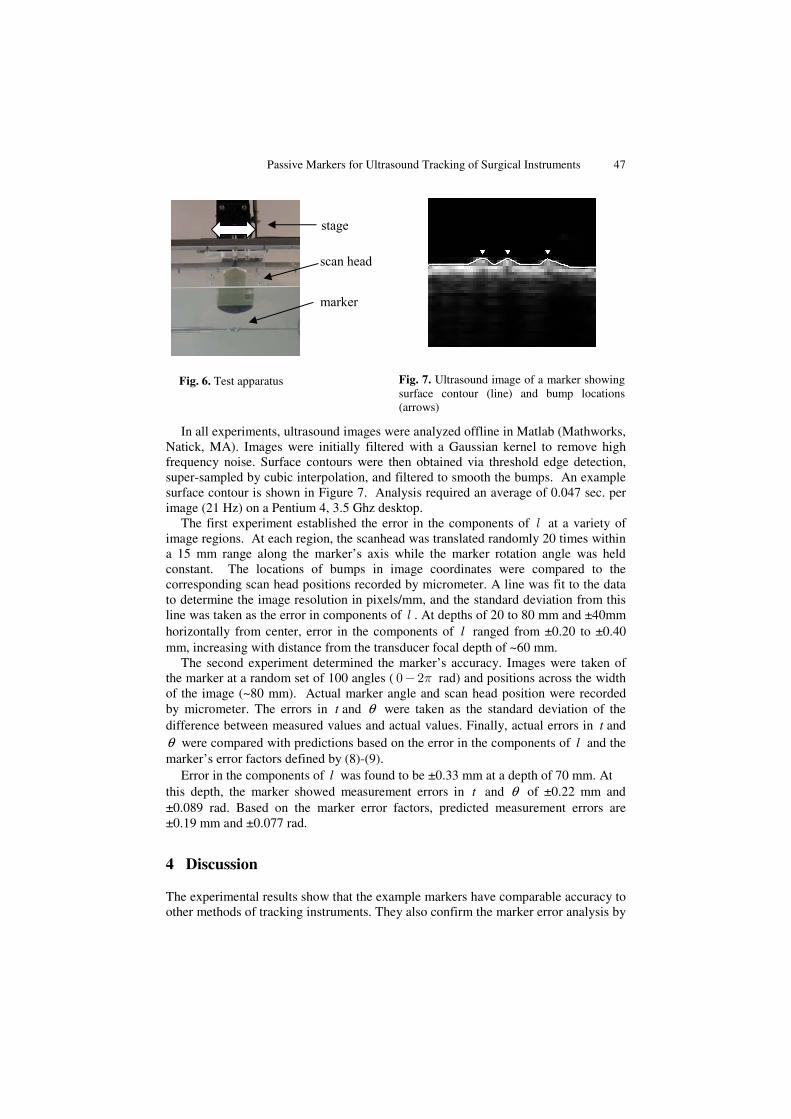
Two imaging experiments were performed to determine the example marker’s accuracy and verify its predicted error factor. Images were generated using a 3.5 MHz 2D ultrasound probe (Analogic, Peabody, MA). The scan head was mounted to a linear micrometer stage over a tank filled with degassed water. A rotational micrometer was fixed to the side of the tank, and a 5mm diameter stainless steel rod, simulating the shaft of a surgical instrument, was attached such that it extended into the imaging plane and could rotate about its axis. The markers were then placed on the rod for imaging. The complete test apparatus is shown in figure 6.

0 1 2 3 4 5 6

0

5

10

15

20

25

(rad)θ

( )θf(mm)

0 1 2 3 4 5 6

0

5

10

15

20

25

(rad)θ

( )θf(mm)

5 10 15 20 25 30 350

0.2

0.4

0.6

0.8

1

1.2

1.4

1.6

1.8

2

θt

(rad/mm)

marker length (mm)

5 10 15 20 25 30 350

0.2

0.4

0.6

0.8

1

1.2

1.4

1.6

1.8

2

θt

(rad/mm)

marker length (mm)

Fig. 4. Plot of ( )θf versus for the example

marker

Fig. 5. Error factor versus length for the

example marker

Passive Markers for Ultrasound Tracking of Surgical Instruments 47

In all experiments, ultrasound images were analyzed offline in Matlab (Mathworks, Natick, MA). Images were initially filtered with a Gaussian kernel to remove high frequency noise. Surface contours were then obtained via threshold edge detection, super-sampled by cubic interpolation, and filtered to smooth the bumps. An example surface contour is shown in Figure 7. Analysis required an average of 0.047 sec. per image (21 Hz) on a Pentium 4, 3.5 Ghz desktop.

The first experiment established the error in the components of l at a variety of image regions. At each region, the scanhead was translated randomly 20 times within a 15 mm range along the marker’s axis while the marker rotation angle was held constant. The locations of bumps in image coordinates were compared to the corresponding scan head positions recorded by micrometer. A line was fit to the data to determine the image resolution in pixels/mm, and the standard deviation from this line was taken as the error in components of l . At depths of 20 to 80 mm and ±40mm horizontally from center, error in the components of l ranged from ±0.20 to ±0.40 mm, increasing with distance from the transducer focal depth of ~60 mm.

The second experiment determined the marker’s accuracy. Images were taken of the marker at a random set of 100 angles ( 0 2π− rad) and positions across the width of the image (~80 mm). Actual marker angle and scan head position were recorded by micrometer. The errors in t and θ were taken as the standard deviation of the difference between measured values and actual values. Finally, actual errors in t and θ were compared with predictions based on the error in the components of l and the marker’s error factors defined by (8)-(9).

Error in the components of l was found to be ±0.33 mm at a depth of 70 mm. At this depth, the marker showed measurement errors in t and θ of ±0.22 mm and ±0.089 rad. Based on the marker error factors, predicted measurement errors are ±0.19 mm and ±0.077 rad.

4 Discussion

The experimental results show that the example markers have comparable accuracy to other methods of tracking instruments. They also confirm the marker error analysis by

stage

scan head

marker

Fig. 6. Test apparatus Fig. 7. Ultrasound image of a marker showing surface contour (line) and bump locations (arrows)

48 J. Stoll and P. Dupont

showing a small difference between actual and predicted measurement errors. Higher image resolutions and higher probe frequencies will likely lower the error in the components of l and thereby increase marker accuracy.

The results also verify that marker analysis can be accomplished with simple image processing. More sophisticated approaches, such as physics-based techniques, may produce further reductions in error.

The family of markers proposed in this paper is also amenable to 3D ultrasound imaging. In particular, it removes the constraint of 2D imaging that the instrument shaft be aligned with the image plane. Since the 3D analysis will be comparable to the 2D approach, the marker accuracy demonstrated with 2D images will likely be the same for 3D images which possess the same error in the components of l .

In conclusion, the markers presented have been shown to be a simple, cost-effective, and accurate approach to image-based instrument guidance. Acknowledgment. This research was funded by the NIH, grant #R01 HL073647.

References

1. Cannon, J et al.: Application of Robotics in Congenital Cardiac Surgery, Seminars in Thoracic and Cardiovascular Surgery: Pediatric Cardiac Surgery Annual. 6(1):72-83, 2003.

2. Nichols, K. et al.: Changes in ultrasonographic echogenicity and visibility of needles with changes in angles of insonation. J Vasc Interv Radiol. 14(12):1553-7 Dec. 2003.

3. Novotny, P., J. Cannon, and R. Howe: Tool Localization in 3D Ultrasound Images. MICCAI, 2003.

4. Lindseth F. et al.: Probe Calibration for Freehand 3-D Ultrasound. Ultrasound in Med. & Biol. 29(11):1607-1623, 2003.

5. Leotta D.: An Efficient Calibration Method for Freehand 3-D Ultrasound Imaging Systems. Ultrasound in Med. & Biol. 30(7):999-1008, 2004.

6. Merdes, C. and P. Wolf: Locating a Catheter Transducer in a Three-Dimensional Ultrasound Imaging Field. IEEE trans Biomed Eng Dec. 2001.

7. Galloway, R. et al.: The accuracies of four stereotactic frame systems: an independent assessment. Biomed Instrum Technol 25(6):457-60 Nov-Dec 1991.

8. Fichtinger, G. et al.: Robotically Assisted Percutaneous Local Therapy and Biopsy. ICAR 2001.