1

POD 3-D PARTICLE TRACKING MODELING STUDY

Particle Tracking Model Testing and Applications Report

Prepared For:

Interagency Ecological Program

Prepared By:

Edward S. Gross, Ph.D., Michael L. MacWilliams, Ph.D.,

Christopher D. Holleman, Thomas A. Hervier

May 11, 2010

2

[This page intentionally left blank.]

3

Executive Summary

The motivation for this study is the observed decline of delta smelt and other pelagic organisms of the upper San Francisco Estuary. Three general factors identified to explain lower pelagic productivity are 1) toxic effects; 2) exotic species effects; and 3) water project effects (Resources Agency, 2007). For each of these factors, the location and movement of delta smelt are likely to be critical for understanding the reasons for the pelagic organism decline (POD) and the efficacy of any actions taken to sustain pelagic fish populations.

In order to investigate the location and movement of delta smelt within the Delta, a three-dimensional hydrodynamic model was applied to simulate hydrodynamics in the Sacramento-San Joaquin Delta, and the hydrodynamic results were used with a particle tracking model to investigate delta smelt distribution and behavior. The Bay-Delta UnTRIM model developed for this project (MacWilliams et al., 2008) builds on previous applications (e.g., MacWilliams and Gross, 2007), and is the first three-dimensional hydrodynamic model extending from the Pacific Ocean through the entire Sacramento-San Joaquin Delta.

The Flexible Integration of Staggered-grid Hydrodynamics Particle Tracking Model (FISH-PTM) was developed to represent particle transport processes for a class of hydrodynamic models. The FISH-PTM is written in portable Fortran 90 and has several capabilities that make it appropriate for the POD-3D project, including:

• Representation of horizontal and vertical transport processes • Flexible particle release capabilities • Representation of movement of particles through structures including culverts and weirs • Representation of particle losses at exports and agricultural diversions • Parallel implementation using OpenMP • Vertical swimming behavior • Flexible post-processing tools • Visualization capabilities using RmaSim

This report documents the formulation, testing and applications of a three-dimensional particle tracking model developed for the POD-3D project. The report includes a discussion of the governing equations for hydrodynamics and particle tracking and the numerical method of the particle tracking model. The results of several test cases are documented and discussed.

The particle tracking model was then applied to an intermodel comparison with the DSM2 PTM and RMATRK. Many similarities are noted among models. However, substantial differences between the DSM2 PTM and the FISH-PTM were noted. These differences include lower estimated entrainment for DSM2 PTM relative to the FISH-PTM for particle release locations in the central Delta. In addition, particles from many release locations arrive more rapidly at Martinez for the DSM2 PTM simulations than the RMATRK and FISH-PTM simulations.

Larval and juvenile delta smelt distribution and regional hatching rates were predicted and compared with observations for 1999 and 2007. Good prediction of observed trends was achieved for 1999. Three different upward swimming scenarios were simulated which generally yielded similar results to the passive scenario. The fates of the population of delta smelt hatched in 1999 were estimated. An annual percent loss of 2% to 3% as a result of entrainment by water

4

projects was estimated, which is substantially lower than the estimate of 8% by Kimmerer (2008).

Fates of particles are calculated for each of the 26 regions from the particle tracking scenario simulations. Again the vertical migration behaviors are found to have little effect on the fate estimates. The calculated fates were found to depend strongly on Delta hydrology and operations during the simulation periods.

5

Abbreviations

2D Two-Dimensional 3D Three-Dimensional CCWD Contra Costa Water District CVP Central Valley Project DCC Delta Cross Channel DICU Delta Island Consumptive Use DFG Department of Fish and Game DWR Department of Water Resources DSM2 PTM Delta Simulation Model 2 Particle Tracking Model EC Electrical Conductivity IEP Interagency Ecological Program FISH-PTM Flexibile Integration of Staggered grid Hydrodynamics Particle Tracking Model NBA North Bay Aqueduct OMR Old and Middle River POD Pelagic Organism Decline PTM Particle Tracking Model RMATRK Resource Management Associates Particle Tracking Model SWP State Water Project TRIM Tidal, Residual, Intertidal & Mudflat Model UnTRIM Unstructured Tidal, Residual, Intertidal & Mudflat Model USACE United States Army Corps of Engineers USBR United States Bureau of Reclamation USGS United States Geological Survey UTM Universal Transverse Mercator

6

1 Introduction

The motivation for this study is the observed decline of delta smelt and other pelagic organisms of the upper San Francisco Estuary. Three general factors were identified to explain lower pelagic productivity: 1) toxic effects; 2) exotic species effects; and 3) water project effects (Resources Agency, 2007). For each of these factors, the location and movement of delta smelt are likely to be critical for understanding the reasons for the pelagic organism decline (POD) and the efficacy of any actions taken to sustain pelagic fish populations.

In order to investigate the location and movement of delta smelt, a three-dimensional hydrodynamic model was applied to simulate hydrodynamics in the Sacramento-San Joaquin Delta, and the hydrodynamic results were used with a particle tracking model to investigate delta smelt hatching, distribution and entrainment. Using hydrodynamics output from the UnTRIM Bay-Delta model (MacWilliams et al., 2008) for periods during the spring and summer of 1999 and 2007, several particle tracking scenarios are simulated to achieve the goals of the POD-3D project. Additional particle tracking scenarios in Clifton Court Forebay will be documented separately.

This report is divided into seven major sections:

• Section 1. Introduction. This section presents the project approach and objectives, as well as a summary of the scope and organization of the report.

• Section 2. Model Formulation. This section discusses the governing equations of three-dimensional hydrodynamics and particle transport and the numerical method of the FISH-PTM.

• Section 3. Model Testing. This section documents the results of several test cases. • Section 4. Intermodel Comparisons. This section discusses simulation of particle

releases in the San Francisco Estuary using the FISH-PTM and two additional particle tracking models, each of which is associated with a different hydrodynamic model.

• Section 5. Delta Smelt Hatching Distribution Simulations. This section discusses particle tracking scenarios of delta smelt distribution in 1999 for passive particles and particles with vertical migration behavior. Delta smelt distribution is simulated in 2007 with a passive particle tracking scenario. The predicted distributions are compared with 20-mm survey data and salvage data from at the Tracy Fish Facility.

• Section 6. Delta Smelt Fate Simulations. This section discusses particle tracking simulations of delta smelt fate in 1999 and 2007 for passive particles and particles with vertical migration behavior. The effect of natural mortality is also estimated to provide additionalcontext for the particle fate predictions.

• Section 7. Summary and Conclusions. This section summarizes the formulation and testing of the FISH-PTM and suggests additional test cases for further evaluation of the model. The results of the particle tracking scenarios simulations are discussed and several conclusions regarding the capabilities of the model, delta smelt hatching distribution and entrainment, and uncertainties in simulations of delta smelt distribution and entrainment are reached.

7

2 Model Formulation

The Flexible Integration of Staggered-grid Hydrodynamics Particle Tracking Model (FISH-PTM) was developed to represent particle transport processes for many staggered grid models. The model can be applied to a variety of staggered grid structures meeting the description of Arakawa C grids (Arakawa and Lamb, 1977), which include some Cartesian grids, curvilinear grids and unstructured grids consisting of triangles and quadrilaterals. The unstructured grid structure of UnTRIM, which involves a mixture of triangles and quadrilaterals, is the most general of these Arakawa C grid structures. The model can also be applied with a variety of vertical grid structures including z-levels, sigma-levels and other stretched vertical coordinates. At the time of the writing of this report, the FISH-PTM has been applied with TRIM, UnTRIM, SUNTANS and GETM.

In the POD-3D project, The UnTRIM Bay-Delta model (MacWilliams et al., 2008) supplies hydrodynamic information, including three-dimensional velocity and eddy diffusivity distributions, to the FISH-PTM. For this reason, the numerical method of the UnTRIM hydrodynamic model (Casulli, 1990; Casulli and Zanolli, 2002) is discussed briefly.

2.1 The UnTRIM Hydrodynamic Model The primary hydrodynamic model used in this technical study was the three-dimensional UnTRIM model (Casulli and Zanolli, 2002). A complete description of the governing equations, numerical discretization, and numerical properties of UnTRIM is provided in Casulli and Zanolli (2002, 2005), Casulli (1999), and Casulli and Walters (2000).

The UnTRIM model solves the three-dimensional Navier-Stokes equations (Equation 2.1 through 2.4) on an unstructured grid in the horizontal plane. The boundaries between vertical layers are at fixed elevations, and cell heights can be varied vertically to provide increased resolution near the surface or other vertical locations. Volume conservation is satisfied by a volume integration of the incompressible continuity equation (Equation 2.4), and the free-surface is calculated by integrating the continuity equation over the depth (Equation 2.5), and using a kinematic condition at the free-surface as described in Casulli (1990). The numerical method allows full wetting and drying of cells in the vertical and horizontal directions. The governing equations are discretized using a finite difference – finite volume algorithm. The discretization of the governing equations and model boundary conditions are presented in detail by Casulli and Zanolli (2002) and is not reproduced here.

The UnTRIM model solvers the three-dimensional momentum equations for an incompressible fluid

⎟⎠⎞

⎜⎝⎛

∂∂

∂∂

+⎟⎟⎠

⎞⎜⎜⎝

⎛∂∂

+∂∂

+∂∂

−=−∂∂

+∂∂

+∂∂

+∂∂

zu

zyu

xu

xpfv

zuw

yuv

xuu

tu vh νν 2

2

2

2

(2.1)

⎟⎠⎞

⎜⎝⎛

∂∂

∂∂

+⎟⎟⎠

⎞⎜⎜⎝

⎛∂∂

+∂∂

+∂∂

−=+∂∂

+∂∂

+∂∂

+∂∂

zv

zyv

xv

ypfu

zvw

yvv

xvu

tv vh νν 2

2

2

2

(2.2)

8

g

zw

zyw

xw

zp

zww

ywv

xwu

tw vh −⎟

⎠⎞

⎜⎝⎛

∂∂

∂∂

+⎟⎟⎠

⎞⎜⎜⎝

⎛∂∂

+∂∂

+∂∂

−=∂∂

+∂∂

+∂∂

+∂∂ νν 2

2

2

2

(2.3)

where ( )tzyxu ,,, and ( )tzyxv ,,, are the velocity components in the horizontal x - and y -directions, respectively; ( )tzyxw ,,, is the velocity component in the vertical z - direction; t is time; ( )tzyxp ,,, is the normalized pressure defined as the pressure divided by a constant reference density; f is the Coriolis parameter; g is the gravitational acceleration; and hν and vν are the coefficients of horizontal and vertical eddy viscosity, respectively (Casulli and Zanolli, 2002). Conservation of volume is expressed by the continuity equation for incompressible fluids

.0=∂∂

+∂∂

+∂∂

zw

yv

xu

(2.4)

The free-surface equation is obtained by integrating the continuity equation (2.4) over depth and using a kinematic condition at the free-surface (Casulli and Zanolli, 2002)

,000

=⎥⎦⎤

⎢⎣⎡

∂∂

+⎥⎦⎤

⎢⎣⎡

∂∂

+∂∂

∫∫ −−vdz

yudz

xt HH

ηηη (2.5)

where ( )yxH ,0 is the prescribed bathymetry measured downward from the reference elevation and ),,( tyxη is the free-surface elevation measured upward from the reference elevation. Thus, the total water depth is given by ( ) ( ) ),,(,,, 0 tyxyxHtyxH η+= .

The governing equation for salt transport (Casulli and Zanolli, 2002) is ( ) ( ) ( )

⎟⎠⎞

⎜⎝⎛

∂∂

∂∂

+⎟⎟⎠

⎞⎜⎜⎝

⎛∂∂

∂∂

+⎟⎠⎞

⎜⎝⎛

∂∂

∂∂

=∂

∂+

∂∂

+∂∂

+∂∂

zs

zys

yxs

xzws

yvs

xus

ts

vhh εεε (2.6)

where s is the scalar concentration; εh is the horizontal diffusion coefficient; and εv is the vertical diffusion coefficient. Turbulent mixing is represented by eddy viscosity and eddy diffusivity coefficients determined by a generic length-scale (GLS) turbulence closure (Umlauf and Burchard, 2003). A more complete description of the governing equations of the UnTRIM model used in the POD-3D project is provided by MacWilliams et al. (2008). The UnTRIM Bay-Delta model is a three-dimensional hydrodynamic and salinity model of San Francisco Bay and the Sacramento-San Joaquin Delta, which extends from the Pacific Ocean through the entire Sacramento-San Joaquin Delta (MacWilliams et al., 2008). The UnTRIM Bay-Delta model has been used in studies of San Francisco Bay and the Sacramento-San Joaquin Delta for California DWR, USBR, USGS, and the US Army Corps of Engineers. The model calibration and validation conducted as part of these studies demonstrate that the UnTRIM Bay-Delta model is accurately predicting flow, stage, and salinity in San Francisco Bay and the Sacramento-San Joaquin Delta under a wide range of hydrologic conditions. Hydrodynamic model output from the UnTRIM Bay-Delta model is the primary source of hydrodynamic results for the FISH-PTM simulations presented in Sections 4 through 6.

9

2.2 Governing Equations of Particle Tracking Model 

The theoretical aspects of particle tracking are discussed in detail by Dunsbergen (1994) and other sources and will not be covered here. However, it should be noted that the derivation of the equations typically used for particle tracking involve assumptions related to diffusion in order to replace a tensor containing nine components of diffusion with an isotropic horizontal diffusion coefficient and a vertical diffusion coefficient.

The stochastic equation describing particle transport is typically referred to as the three-dimensional Fokker-Plank equation, but should be referred to more precisely as the Ito-Fokker-Plank equation to emphasize that the Ito integration rule has been used (Dunsbergen, 1994). The Lagrangian model that corresponds to the Fokker-Plank equation using the Ito integration rule can be written as

, 2 (2.7)

where i is the coordinate dimension, Xi is the particle position in the i dimension, ui is the velocity in the i dimension, X = (X1,X2,X3) is the position of the particle, t is time, Di is the diffusion coefficient in the i dimension, dt is the time step of integration, R is a uniformly distributed number between -1 and 1, and r = 1/3 (Stijnen et al., 2006; Visser, 1997). The gradient of Di is evaluated at the location X and time t, while the value of Di in the last term of Equation 2.7 is evaluated at the location (X + 0.5 ) and time t. Isotropic horizontal diffusion

(D1 = D2 = hε ) is assumed and the vertical diffusion (D3 = vε ) is specified by the eddy diffusivity determined by the GLS turbulence closure (Umlauf and Burchard, 2003).

2.3 Formulation of Particle Tracking Model 

The FISH-PTM solves Equation 2.7 in a manner which, as closely as is feasible, retains consistency with the numerical solution of Equation 2.6 in UnTRIM and many other staggered (Arakawa C) grid hydrodynamic models.

The numerical solution of particle trajectories follows a commonly used operator-split methodology in which the governing equation is solved in independent steps (e.g., Dunsbergen, 1994). The particle tracking algorithm consists of four individual steps

• Horizontal advection • Vertical advection • Horizontal diffusion • Vertical diffusion

Computing particle trajectories in multiple steps greatly simplifies the evaluation of particle trajectories and, therefore, improves computational efficiency.

The horizontal particle advection trajectory in each grid cell is calculated according to , (2.8)

for the horizontal dimensions (i = 1, 2). Equation 2.8 represents advection in the horizontal dimension and, therefore, corresponds to a portion of Equation 2.7. For each FISH-PTM time step, horizontal advection is applied in one or more steps. The particle moves at the velocity

10

interpolated to the particle location until a cell boundary is encountered. If a cell boundary is encountered, the interpolated advection velocity is recalculated using the node velocities of the grid cell entered. Because each substep of the horizontal advection is a linear trajectory, the horizontal advection algorithm is quite simple and computationally efficient.

In order to determine particle trajectories, the velocity field calculated by the hydrodynamic model must be interpolated to each particle location. The velocities calculated by a staggered grid hydrodynamic model are normal velocities to each cell side. Node velocities are calculated for each grid cell from the side-normal velocities. The velocity field defined at the nodes is then interpolated to the particle location. The following bilinear interpolation method applies to both triangles and quadrilaterals (Ketefian, 2006) , (2.9)

where x and y are the coordinates of the particle, , is the interpolated velocity component, and a, b, c, and d are interpolation coefficients determined for the grid cell (triangle or quadrilateral). The interpolation coefficients depend only on the geometry of the cell. In practice, this equation is manipulated so that a weight is applied to the velocity determined at each node of a cell. The sum of the individual node weights is 1. On triangles, d = 0, and this method corresponds to use of standard linear shape functions in finite element methods. On quadrilaterals, the interpolation can lead to node weights not bounded by [0 1] for some specific geometries, most notably “diamond” shaped quadrilaterals, such as square grid cells with all side alignments corresponding to 45 degrees rotation from the coordinate axes. In the rare cases in which the calculated node weights corresponding to Equation 2.9 are not bounded by [0 1], an inverse distance weighting of node velocities is applied.

The vertical advection is calculated in an analogous manner but is less complex because the vertical velocities are simply interpolated linearly from the top and bottom faces of the cell to the particle location. The swimming velocity attributed to particles is added to the hydrodynamic velocity interpolated to the particle position.

The vertical diffusion is calculated using the method of Ross and Sharples (2004) which avoids common “pitfalls” that can lead to large errors in particle distribution (Ross and Sharples, 2004). Multiple aspects of the method outlined by Ross and Sharples (2004) are reflected in Equation 2.7. First Equation 2.7 includes a correction term for spatial variations in diffusion. This term is not present in some “naïve” particle tracking methods, leading to accumulation of particles in low diffusivity regions (Visser, 1997). In addition, the diffusion coefficient is evaluated at the location 0.5 ) instead of X. While the location of evaluation of the diffusion coefficient is not intuitive, this approach is required to maintain consistency with Equation 2.6 (Visser, 1997). The vertical diffusion is applied in several substeps using the time step criterion of Ross and Sharples (2004).

The horizontal diffusion is treated similarly. However, unlike the vertical diffusivity, the horizontal diffusivity is not typically calculated by the hydrodynamic model. Horizontal diffusivity is not required by many estuary and ocean models because the most important transport processes are explicitly resolved. In addition, some numerical diffusion is present in the scalar (e.g., salt) transport method. For both of these reasons, hydrodynamic model results are often insensitive to specified values of horizontal diffusivity and/or other sub-grid scale mixing of reasonable magnitude. However, since there is no numerical diffusion associated with the

11

particle tracking approach, the FISH-PTM applies a horizontal diffusion coefficient to represent all sub-grid scale processes. This coefficient is calculated by the following equation commonly used to represent horizontal turbulence (2.10)

where C is a user specified constant, H is water column depth and U* is the friction velocity (Fischer et al., 1979). Equation 2.10 is evaluated to determine a depth-averaged value of the horizontal diffusion coefficient at each node. The horizontal diffusion coefficient is interpolated to the particle location using the same method used to interpolate horizontal velocity (Equation 2.9). The derivative of Equation 2.10 in the x and y direction is evaluated in order to determine the gradient of horizontal diffusion.

12

3 Model Testing

The FISH-PTM has been applied to simulate particle transport for test cases with known solutions. The objective of the test cases is both to show that the model predictions are accurate and to check for any unphysical artifacts in the particle tracking results that may result from the numerical formulation of the particle tracking method. The test cases include simple one-dimensional advection and diffusion test cases using specified velocity fields and diffusion coefficients and more complex two-dimensional and three-dimensional test cases using TRIM and UnTRIM hydrodynamic results.

3.1 One­dimensional Test Cases 

3.1.1 Advection in a Linearly Increasing Velocity Field Perhaps the most fundamental test case of any particle tracking model is the ability of the model to move particles at the correct velocity in a specified one-dimensional velocity field. Put most simply, this test case assesses whether particles move at the correct speed. In this test case, a linearly varying velocity field is specified (Figure 3-1). The velocity field is representative of both the shape and magnitude of typical vertical velocity profiles in estuarine hydrodynamics simulations.

Figure 3-1 Specified velocity field for advection test case.

0

1

2

3

4

5

6

7

8

9

10

0 0.0002 0.0004 0.0006 0.0008 0.001 0.0012

Distance [m

]

Velocity [m/s]

13

The velocity field shown in Figure 3-1 can easily be integrated to calculate the analytical (exact) solution for the particle trajectory. The vertical advection portion of the FISH-PTM simulated this trajectory using a time step of 90 seconds, which is typical for FISH-PTM simulations of estuarine transport. The particles are released at a position of 0.25 meters and after 10 hours are located at 9.01 meters (Figure 3-2), compared with an exact solution of 9.15 meters. The FISH-PTM transports particles approximately the correct distance, with an error in position of 1.6%.

The predicted trajectory does not more precisely match the analytical solution because a simple and computationally efficient advection method is used. In contrast, a more precise but more computationally intensive method, known as “streamline tracking” (e.g. Ham et al., 2006), would exactly match the analytical solution (to machine precision) for this velocity field independent of the time step chosen for the integration. Streamline tracking has been implemented in the FISH-PTM for vertical transport and also for horizontal transport on a Cartesian grid structure, however, is not currently an option for horizontal transport on unstructured grids.

Figure 3-2 Analytical and predicted particle trajectory for linear velocity profile test case.

3.1.2 Constant Diffusion Coefficient The second test case assesses the accuracy of the representation of diffusion in the FISH-PTM. This test case is a one-dimensional diffusion test case for a point release of particles with uniform diffusion coefficient of 0.0001 m2 s-1, which is within in the range of typical vertical eddy diffusivity values in of the San Francisco Estuary. A set of 100,000 particles were released at a distance (z coordinate) of 5 meters and tracked over 3 hours. The analytical solution for this test case is a Gaussian distribution with a variance of 2Kt, where t is the time from release of the particle. In Figure 3-3, the variance of the group of particles simulated is compared with the analytical solution. The predicted particle distribution three hours after the particle release is

0

1

2

3

4

5

6

7

8

9

10

0 2 4 6 8 10

Distance [m

]

Time From Release [hours]

Analytical

Predicted

14

compared with the Gaussian analytical solution in Figure 3-4. The predicted results for the constant diffusion test case closely match the analytical solution.

Figure 3-3 Analytical and predicted particle distribution variance for constant diffusivity test case.

0

0.5

1

1.5

2

2.5

0 1 2 3

Variance [m

2 ]

Time From Release [hours]

Analytical

Predicted

15

Figure 3-4 Predicted and analytical particle distribution histogram for constant diffusivity test case.

3.1.3 Maintenance of Well­mixed Conditions Many Lagrangian models of diffusion suffer from a severe artifact in which particles concentrate in regions of low diffusivity. This artifact, discussed in detail by Visser (1997), can have particularly severe effects in stratified region in which the vast majority of particles will aggregate in the low diffusivity regions. As mentioned previously, this paper follows the approach of Ross and Sharples (2004) to eliminate this artifact. The test case used by Visser (1997) and Ross and Sharples (2004) is repeated here for the FISH-PTM. This case uses a high-order polynomial distribution of vertical (eddy) diffusion coefficient, shown in Figure 3-5.

For this test case, the FISH-PTM is seeded with 100,000 uniformly distributed particles over the 40 meter deep water column and the particle distribution is simulated for 1 day. As shown in Figure 3-6, the well-mixed conditions are still present at the end of the simulation. The maintenance of well-mixed conditions relies on several aspects of the approach of Ross and Sharples (2004). The FISH-PTM allows interpolation of eddy diffusivity and evaluation of eddy diffusivity gradients from a cubic spline approach, as suggested by Ross and Sharples (2004). However, the results in Figure 3-6 are achieved by a simpler and more computationally efficient approach using a piecewise linear description of eddy diffusivity.

The FISH-PTM accurately preserves well-mixed conditions, avoiding a common artifact that concentrates particles in low diffusivity regions.

0

2000

4000

6000

8000

10000

12000

14000

16000

0 1 2 3 4 5 6 7 8 9 10

Num

ber o

f Particles

Distance [m]

Analytical

Predicted

16

Figure 3-5 Eddy diffusivity profile representative of wind- and tide-induced mixing.

Figure 3-6 Predicted and analytical particle distribution histogram for variable diffusivity test case.

0

5

10

15

20

25

30

35

40

0.0000 0.0100 0.0200 0.0300

Distance above Bed

 [m]

Diffusion Coefficient [m2/s]

0

5

10

15

20

25

30

35

40

0 500 1000 1500 2000 2500 3000

Distance from

 Bed

 [m]

Number of Particles

Analytical

Predicted

17

3.2 Multi­Dimensional Test Cases 

3.2.1 Horizontal Advection in a Uniform Straight Channel Flow This test case simulates particle transport under steady flow in a straight uniform channel. The test case channel is straight with a uniform depth of 10 meters. The channel width is 1,000 meters and an inflow of 10,000 m3 s-1 (cms) is specified at the upstream end. This case uses only the horizontal advection term of Equation 2.7. Hydrodynamic model results for this test case are provided by the TRIM model (not UnTRIM) using a Cartesian grid with horizontal grid spacing of 1,000 meters and a single vertical layer to yield a depth-averaged model. The particles are released on the centerline of the channel at x = 10,000 meters, near the upstream end of the domain.

Since the domain is also one cell wide, the simulation is a one dimensional channel flow simulation. The test case is considered a “multi-dimensional test case” only because it tests the multi-dimensional horizontal advection algorithm of the FISH-PTM particle tracking model.

The particles move downstream at a constant velocity (Figure 3-7) of 1 m s-1. The correct time to reach x = 90,000 meters is 22.2 hours and the predicted time for particles to pass this location is also 22.2 hours after the release time. Thus, in this simple velocity field, the FISH-PTM moves particles at the correct speed.

Figure 3-7 Predicted particle trajectory for straight steady channel flow test case.

3.2.2 Horizontal Advection and Vertical Diffusion in Uniform Straight Channel Flow  In a steady open channel flow, the vertical velocity distribution is approximately logarithmic and the vertical eddy diffusivity follows roughly a parabolic distribution (Nezu and Rodi, 1986). These approximations allow a simple and well-known estimate of longitudinal dispersion from

0

20

40

60

80

100

120

0 6 12 18 24

Distance [m

]

Time From Release [hours]

Analytical

Predicted

18

shear dispersion of K = 5.93HU*, where U* is the friction velocity (Fischer et al., 1979). The same depth and flow speed are chosen as in the previous test case, specifically H = 10 meters and U* = 0.68 m s-1. Therefore, the estimated K from the analytical relationship is 4.00 m2 s-1.

The horizontal grid from the previous test case was used with a vertical grid spacing of 0.25 meters. In this test case, the analytical approximations of velocity profile and eddy diffusivity are input to the FISH-PTM so that the spread of particles can be compared with those expected from the analytically determined shear dispersion. The variance of the particle distribution increases approximately linearly in time (Figure 3-8), and the dispersion coefficient estimated from the particle distribution 24 hours after the particle release is 4.05 m2 s-1. Therefore, the horizontal spreading (dispersion) rate of particles resulting from the sheared vertical velocity is predicted accurately.

Figure 3-8 Predicted variance of particle distribution for shear dispersion test case.

3.2.3 Advection in a Curved Channel Flow  This test case simulates particle transport under steady flow in a “racetrack” channel with two straight sections and one curved section using the three-dimensional hydrodynamic model UnTRIM to supply hydrodynamics. Unlike the previous test cases which used simple uniform grid structures, the grid for this test case is composed of triangles of varying size and orientation. Therefore, this test case assesses the ability of the FISH-PTM to move (advect) particles at the correct velocity in a domain with a non-uniform grid. Due to the circulation pattern in the curved section of the domain, some particles will arrive at the lateral boundaries of the channel. Therefore, in addition to providing another quantitative test case of advection, this test-case is also intended to check for artifacts (e.g., “sticking”) related to movement along lateral boundaries. If any artificial sticking is present in particle tracking simulations, it would result in

0

100000

200000

300000

400000

500000

600000

700000

800000

0 6 12 18 24

Variance [m

2 ]

Time From Release [hours]

Analytical

Predicted

19

biased particle advection with particles moving at a lower speed than the corresponding local water velocity.

The channel is straight with a uniform depth of -10 meters. The vertical grid spacing is 1 meter. A free-surface elevation of zero is enforced at the downstream boundary, leading to a depth of 10 meters at that location and slowly increasing depth upstream. The channel has a uniform width of 120 meters. The UnTRIM grid for this case consists entirely of triangles. The straight channel portion of the domain consists of equilateral triangles with a side length of 20 meters and the triangles in the curved section are also roughly the same dimensions (Figure 3-9). An inflow of 500 m3 s-1 is applied at the upstream boundary.

This case uses only the horizontal advection term of Equation 2.7. A set of 100 particles are released uniformly distributed across the channel near the upstream end of the “racetrack” channel, at the depth for which the velocity equals the depth averaged velocity (approximately 4 meters from the bed).

The distribution of the particles 4 hours after the release time, shows a strong effect of initial lateral position with the particles released on the inside of the channel ahead of the particles released on the outside of the channel (Figure 3-10). There is no evidence of particles “sticking” to lateral boundaries or any other notable artifacts in the results.

Using the hydraulic residence time methodology discussed previously, the average expected time for the particles to reach x = 3,000 meters on the downstream channel section is 3.80 hours. The particles reach this point between 3.75 hours and 3.95 hours, with an average arrival time of 3.85 hours. The arrival times of the particles are slightly later than expected, probably because the vertical position of the particles in the water column does not exactly correspond to the point where the horizontal velocity is equal to the depth-averaged velocity over the entire length of the channel. For a sensitivity test, particles were also released at mid-depth. In this case, the arrival time of the particles ranges from 3.42 hours to 3.72 hours, with an average arrival time of 3.6 hours. The sensitivity to release depth is largely related to the fact that vertical diffusion is neglected in these simulations.

Figure 3

Figure 3

3.2.4 LThis test trapezoidway a groTwo comregions a

3-9 Model gr

3-10 Particle

ateral Part

case simuladal channel woup of partic

mmon artifacand a uniform

rid for curve

distribution

ticle Distrib

ates lateral pawith a steadycles is distribcts in particlem number of

d channel flo

n 4 hours afte

bution in T

article distriby flow. This buted (“splite tracking mf particles in

ow test case

er particle re

Trapezoida

bution for a test case is p

t”) between/amodels are pan each unit w

.

elease for cur

l Channel 

centerline pparticularly iamong chan

articles accumwidth of a cha

rved channe

 

article releasimportant tonels at a junmulating in lannel, indep

l flow test ca

se in a straigo insure that nction is realilow diffusivendent of w

20

ase.

ght the istic. ity ater

21

depth, resulting in higher volume concentration in shoal regions than channel regions. If any artifacts are present that result in non-uniform volume concentration (particles per unit water volume) of particles when well-mixed conditions are expected, these artifacts would result in inaccurate “splitting” at junctions.

This test case is analogous to the one-dimensional test case for maintenance of well-mixed conditions. As in that case, the terms accounting for the gradient in diffusivity are of critical importance, however, this three-dimensional test case focuses on lateral distribution. In addition to the diffusivity changing in the lateral dimension the depth also varies. The maximum depth of the channel is 10 meters and the minimum depth is 5 meters. Both the flat section and each sloping section are 500 meters wide, as shown in Figure 3-11. The total cross-sectional area is 12,500 m2 and the specified inflow is 12,000 m2, resulting in a cross-sectional average velocity of slightly less than 1 m s-1. For this test case, the value of the coefficient C in Equation 2.10 is chosen to be 0.6, a typical value for natural streams (Fischer et al. 1979). Note that the mixing parameterization described by Equation 2.10 will result in larger mixing coefficients in the deepest part of the trapezoidal channel relative to the sloping sections of the channel. In the test case only particle diffusion is considered. Particle advection is neglected in order to simplify the model boundary conditions.

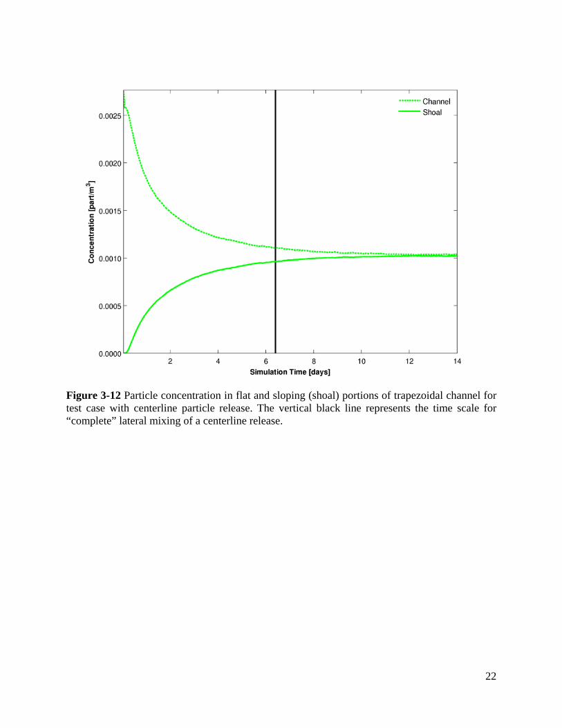
From a physical point of view it is clear that a conservative and passive scalar (e.g., salinity) should eventually become well-mixed in this case. Because the governing equation and implementation of the FISH-PTM is analogous to the scalar transport equation (Equation 2.6), it is also expected that the particle concentration (defined as number of particles per unit volume) will eventually become uniform. The time scale (representative time) for “complete” mixing for a centerline discharge can be approximated by the expression T = 0.1 W2/ where W is the channel width (Fischer et al., 1979). Using a representative value of for the cross-section gives T = 6.4 days.

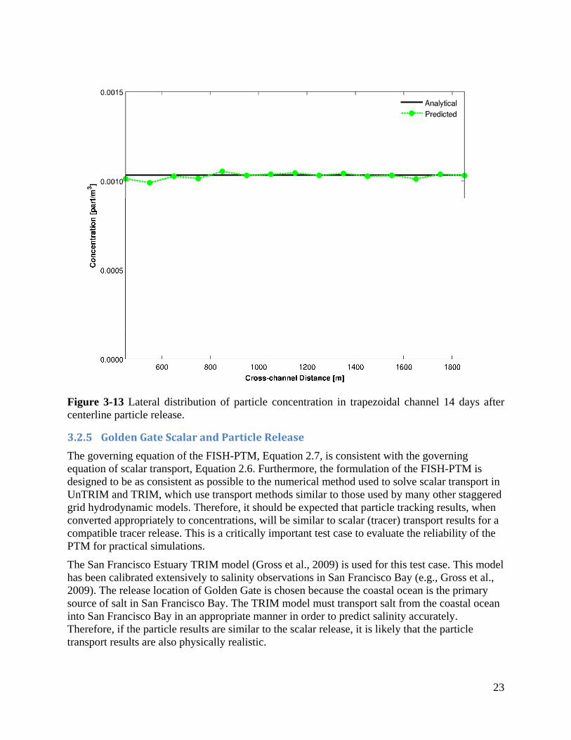
One metric used to judge whether well-mixed behavior is achieved is whether the particle concentration, defined as number of particles per unit volume, in the flat portion of the channel equals the volume concentration in the sloping portions of the trapezoidal channel. Figure 3-12 indicates that near the end of the simulation, roughly equal concentrations are achieved. In addition, Figure 3-13 indicates that concentration is roughly equal in each 100 meter grid cell across the channel at the end of the 14 day simulation.

Figure 3-11 Cross-sectional geometry for trapezoidal channel test case.

22

Figure 3-12 Particle concentration in flat and sloping (shoal) portions of trapezoidal channel for test case with centerline particle release. The vertical black line represents the time scale for “complete” lateral mixing of a centerline release.

23

Figure 3-13 Lateral distribution of particle concentration in trapezoidal channel 14 days after centerline particle release.

3.2.5 Golden Gate Scalar and Particle Release The governing equation of the FISH-PTM, Equation 2.7, is consistent with the governing equation of scalar transport, Equation 2.6. Furthermore, the formulation of the FISH-PTM is designed to be as consistent as possible to the numerical method used to solve scalar transport in UnTRIM and TRIM, which use transport methods similar to those used by many other staggered grid hydrodynamic models. Therefore, it should be expected that particle tracking results, when converted appropriately to concentrations, will be similar to scalar (tracer) transport results for a compatible tracer release. This is a critically important test case to evaluate the reliability of the PTM for practical simulations.

The San Francisco Estuary TRIM model (Gross et al., 2009) is used for this test case. This model has been calibrated extensively to salinity observations in San Francisco Bay (e.g., Gross et al., 2009). The release location of Golden Gate is chosen because the coastal ocean is the primary source of salt in San Francisco Bay. The TRIM model must transport salt from the coastal ocean into San Francisco Bay in an appropriate manner in order to predict salinity accurately. Therefore, if the particle results are similar to the scalar release, it is likely that the particle transport results are also physically realistic.

24

Idealized hydrodynamic forcing is used in this test case to simplify interpretation of results. Steady Net Delta Outflow of 260 m3 s-1 is specified and a repeating daily tide is applied on the coastal boundary. No other forcing is applied.

The TRIM model is run to simulate a point release of scalar mass at a rate of 1,000 kg s-1. The point source is introduced in the surface layer at the center of the Golden Gate cross-section. The flow associated with this point source is 1 m3 s-1, which is negligible compared with tidal flows through this cross-section.

An analogous particle release is specified at the same location with 1 particle per second released and each particle representing 1,000 kg, to result in a 1,000 kg s-1 rate of particle mass release. The streamline tracking option is used for horizontal advection because the shoreline is represented crudely on a Cartesian grid. Streamline tracking reduces the potential for particle tracking artifacts near the shoreline, such as particles sticking in some shoreline areas. All other FISH-PTM settings are identical to the settings used in FISH-PTM applications documented in Sections 4, 5 and 6.

Both particles and scalar mass are “destroyed” when they encounter the open boundary of the model domain, located approximately 22 km west of the Golden Gate. For this reason the total scalar and particle mass does not increase indefinitely, but asymptotically approach tidally-averaged steady-state values after sufficient simulation time.

The scalar mass and particle mass are calculated over a 28 day period in 4 subembayments (coastal ocean, Central Bay, San Pablo Bay and Suisun Bay). In the first several days following the release, nearly all scalar mass and particle mass is located in the coastal ocean and Central Bay with large tidal exchange between these two regions (Figure 3-14 and Figure 3-15). Through the entire simulation period the predicted particle mass in the coastal ocean is nearly equal to the predicted scalar mass in the coastal ocean region (Figure 3-14). Similarly, the predicted particle mass in Central Bay is nearly equal to the predicted scalar mass in Central Bay (Figure 3-15). After several days, significant particle mass and scalar mass enters San Pablo Bay (Figure 3-16). Slightly more predicted scalar mass than particle mass enters San Pablo Bay. Relatively little scalar mass and particle mass enters Suisun Bay, however, the predicted scalar mass is substantially larger than the predicted particle mass in this subembayment (Figure 3-17). Overall the particle tracking results are very similar to the scalar transport results both in tidal variability and long-term trends. The scalar transport results indicate slightly more mixing in the landward direction than the particle tracking results. These differences may result in part from the effects of numerical diffusion associated with the scalar transport simulation.

This is the most important test case presented because it is a simulation of particle transport in the San Francisco Estuary at the time and spatial scales of interest for the POD particle tracking studies. The test case results indicate that the overall transport of particles in the San Francisco Estuary calculated by the FISH-PTM is similar to the transport of a tracer calculated by a calibrated hydrodynamic model.

25

Figure 3-14 Predicted scalar mass and particle mass in the coastal ocean.

Figure 3-15 Predicted scalar mass and particle mass in Central San Francisco Bay.

0.0E+00

1.0E+08

2.0E+08

3.0E+08

4.0E+08

5.0E+08

6.0E+08

7.0E+08

7/2/1993 7/9/1993 7/16/1993 7/23/1993 7/30/1993

Mass [kg]

Scalar

Particle

0.0E+00

1.0E+08

2.0E+08

3.0E+08

4.0E+08

5.0E+08

6.0E+08

7.0E+08

7/2/1993 7/9/1993 7/16/1993 7/23/1993 7/30/1993

Mass [kg]

Scalar

Particle

26

Figure 3-16 Predicted scalar mass and particle mass in San Pablo Bay.

Figure 3-17 Predicted scalar mass and particle mass in Suisun Bay.

0.0E+00

1.0E+08

2.0E+08

3.0E+08

4.0E+08

5.0E+08

6.0E+08

7.0E+08

7/2/1993 7/9/1993 7/16/1993 7/23/1993 7/30/1993

Mass [kg]

Scalar

Particle

0.0E+00

1.0E+08

2.0E+08

3.0E+08

4.0E+08

5.0E+08

6.0E+08

7.0E+08

7/2/1993 7/9/1993 7/16/1993 7/23/1993 7/30/1993

Mass [kg]

Scalar

Particle

27

3.3 Test Case Discussion The FISH-PTM performs well for all of the test cases presented. The four processes represented by the FISH-PTM model are: 1) vertical advection; 2) vertical diffusion; 3) horizontal advection and; 4) horizontal diffusion. Each of these processes is tested individually for test cases with known solutions and the FISH-PTM accurately matches these solutions. These test case results suggest that the particle tracking model accurately represents horizontal and vertical advection and diffusion. Most importantly, particle transport in the FISH-PTM is also found to compare fairly closely to tracer transport simulated with the three-dimensional TRIM hydrodynamic model.

In ongoing work, predicted particle paths are compared with drogue paths in Clifton Court Forebay. Additional testing, including comparison with observations of fish tracked with acoustic tags, drifter data and dye releases would be useful to increase confidence in the FISH-PTM and better define the level of accuracy/reliability associated with the model.

28

4 Intermodel Comparisons

Particle tracking models have been used extensively in applications to the San Francisco Estuary. Results from the various particle tracking models applied to date have not been compared in previous studies. This section describes key results from a comparison of three particle tracking models that are currently applied in the San Francisco Estuary: DSM2 PTM, RMATRK and the FISH-PTM. Each model is driven by different hydrodynamic results. The DSM2 PTM model is driven by one-dimensional hydrodynamic results from the DSM2 model. The RMATRK model is driven by two-dimensional RMA Bay-Delta model results, for which many narrow channels are represented with a one-dimensional approach. The FISH-PTM model is driven by three-dimensional UnTRIM Bay-Delta model (MacWilliams et al. 2008) hydrodynamic results.

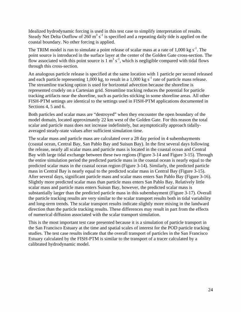
4.1 Intermodel Comparison Scenarios The scenarios for intermodel comparison are representative of how the particle tracking models are used in some POD studies and are designed to provide a clean comparison among models. In some particle tracking simulations for POD studies, particles are released at 20-mm survey stations and tracked through time to estimate entrainment and other particle fates (e.g., Kimmerer and Nobriga, 2008). This approach is followed here with particles released hourly at each of the 20-mm survey stations at an hourly interval for one day to span a range of tidal conditions, and tracked for two months.

For both the FISH-PTM and RMATRK models, 1,000 particles per hour are released at each 20-mm survey station in Suisun Bay and the Delta (Figure 4-1). Due to limitations in the number of particles that can be simulated with DSM2 PTM, only 200 particles per hour were released from DSM2 PTM.

The possible “final” fates for each particle are entrainment into the SWP and CVP and exit past a line in Martinez that corresponds with the boundary of the DSM2 model, reported as “exited Delta.” Particles that are still present at the end of the simulations have not yet reached these “final” fates and are reported as “within Delta.” Particles are not entrained by agricultural diversions in any of the particle tracking simulations for these scenarios.

Two different sets of particle fate calculations are performed with each model. In the first, particles are released on April 28, 1999 and, in the second, particles are released on May 28, 1999. The hydrology changes substantially between these two periods, as indicated by Figure 4-2. Specifically, the San Joaquin flows decrease substantially during the middle of May and the Delta Cross Channel opens on May 28. Exports were substantially larger during July than in April and May. Figure 4-3 compares the net flows averaged from April 28, 1999 to May 28, 1999 to the net flows averaged from May 28, 1999 to June 28, 1999. During the latter averaging period San Joaquin River flows are substantially lower, leading to much larger flows from the central Delta toward the exports. Thus the two different simulation periods span a range of potential entrainment conditions with higher entrainment risk in the second period than the first period.

29

Figure 4-1 Locations of 20-mm survey stations in Suisun Bay and the Delta.

30

Figure 4-2 Key delta outflows during the model intercomparison simulation periods.

Figure 4-3 South Delta and central Delta net flows. The left panel shows net flows in cfs averaged from April 28, 1999 to May 28, 1999. The right panel shows net flows averaged from May 28, 1999 to June 28, 1999.

31

4.2 Particle Release on April 28, 1999 In this scenario particle releases commence at midnight on April 28, 1999 and proceed at an hourly interval for 24 hours. The predicted fates for each model after 2 months of simulation are summarized in Figure 4-4. The various models show similarities in regions where the particle fate could be guessed a priori without use of a particle tracking model. For example, virtually all releases in the western Delta exit the Delta. However, predicted fate in the central Delta and south Delta are substantially different. For example, at station 815, the predicted percentage of particles entrained at all export locations (CVP, SWP, NBA, CCWD) in the 2 month simulation period is 1.55% for the FISH-PTM, 0.65% for RMATRK and 1.04% for DSM2. The percent of particles entrained at water exports for each release location and each particle tracking model during the 2 month simulations for the April 28, 1999 particle releases is reported in Table 4-1.

The differences in particle tracking model predictions at station 815 are examined in more detail by plotting the cumulative percentage of particles entrained as a function of time at different locations. The trends for particles entering Clifton Court Forebay (CCF) (Figure 4-5) are quite different with .5% predicted by the FISH-PTM model, and 0.3% predicted by both RMATRK and the DSM2 PTM in the last week of May. The relatively small number of particles used in the DSM2 PTM simulation makes the DSM2 cumulative entrainment plot appear somewhat jagged. The trends for entrainment by CVP exports at the Tracy pumping plant (Figure 4-6) are also different among all models. The FISH-PTM model entrains more particles in the last week of May. The predicted entrainment by the CVP is lower in the RMATRK simulation (0.5%) and DSM2 PTM simulation (0.3%) than in the FISH-PTM simulation (0.7%). Most of the particles released at station 815 arrive at Martinez by the end of the simulation period (Figure 4-7). However, the time from release to the initial arrival of particles at Martinez is quite different among models. The DSM2 PTM model’s particles start to arrive after roughly 10 days, while at least 12 days are required for the particles to arrive at Martinez in the FISH-PTM and RMATRK simulations.

The first month of the simulation period for the April 28,1999 particle releases is a particularly difficult period for intermodel comparison due to the low average OMR flows (-530 cfs) during the first month of the simulation period (see Figure 4-3). Because these flows are so small, minor absolute differences in predicted net flows among models (e.g. a difference of 200 cfs) could lead to large differences in predicted entrainment.

32

Table 4-1 Percentage of particles entrained at water exports during two month simulation period for April 28, 1999 particle release.

Station  FISH‐PTM  RMATRK DSM2 PTM703  0.00  0.00 0.00704  0.00  0.00 0.00706  0.00  0.00 0.02707  0.00  0.00 0.00711  0.00  0.00 0.02804  0.00  0.00 0.00809  0.02  0.01 0.02815  1.55  0.65 1.04901  4.30  5.43 2.52902  24.54  19.04 5.44906  6.69  4.80 3.94910  28.13  19.02 15.15911  28.13  19.02 15.15912  29.85  23.66 17.69914  65.11  65.70 81.02915  87.15  71.81 69.65918  97.44  95.63 99.13919  4.47  2.25 2.75

33

Figure 4-4 Predicted fates at 20-mm survey stations after two months from particle release, for the April 28, 1999 particle release.

34

Figure 4-5 Cumulative percentage of particles that enter CCF (SWP) as a function of time for the April 28, 1999 particle release.

Figure 4-6 Cumulative percentage of particles entrained by the CVP as a function of time for the April 28, 1999 particle release.

35

Figure 4-7 Cumulative percentage of particles entrained that arrive at Martinez as a function of time for the April 28, 1999 particle release.

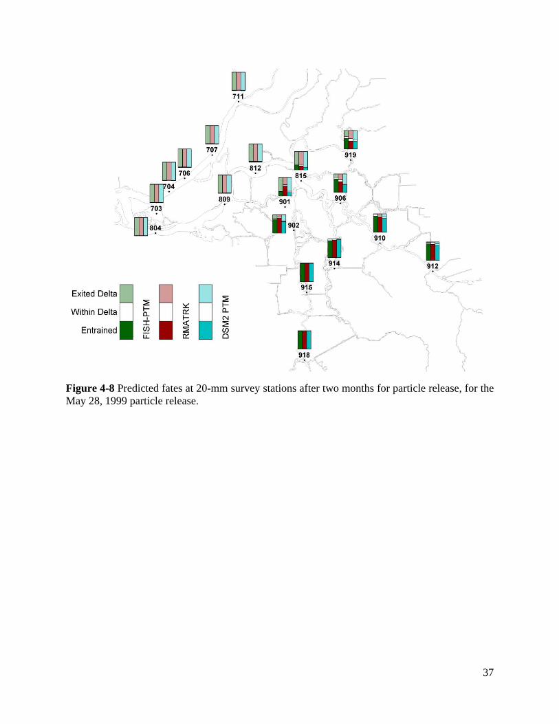
4.3 Particle Release on May 28, 1999 In this scenario, particle releases commence at midnight on May 28, 1999 and proceed at an hourly interval for 24 hours. This release time corresponds to a period of substantially larger (more negative) OMR flows (-2900 cfs average net flow over the month following release), relative to the month following the April 28, 1999 release (-530 cfs average net flow over the month following release). The predicted fates for each model after 2 months of simulation are summarized in Figure 4-8. The various models show some similarities in regions where the particle fate could be guessed a priori without use of a particle tracking model. For example, virtually all releases in the western Delta exit the Delta. However, predicted fate in the central Delta and south Delta are substantially different. For example, at station 815, the predicted percentage of particles entrained at all export locations (CVP, SWP, NBA, CCWD) in the 2 month simulation period is 27.42% for the FISH-PTM, 21.49% for RMATRK and 11.69% for DSM2. The percent of particles entrained at water exports for each release location and each particle tracking model during the 2 month simulations for the May 28, 1999 particle releases is reported in Table 4-2.

The differences in particle tracking model predictions at station 815 are examined in more detail by plotting the cumulative percentage of particles entrained as a function of time at different locations. The trends for particles entering Clifton Court Forebay (CCF) (Figure 4-9) are similar for the FISH-PTM model (7%) and RMATRK model (8%), but predicted entrainment is much lower for the DSM2 PTM model (3%). The trends for entrainment by CVP exports at the Tracy pumping plant (Figure 4-10) are different among all models with the FISH-PTM model entraining the most particles (15%) and RMATRK entraining fewer (11%) and DSM2 PTM

36

entraining the fewest particles (7%). The entrainment predicted by all models is higher for the May 28, 1999 particle release than the April 28, 1999 particle release. This difference occurs primarily because the San Joaquin River inflows decrease dramatically during May of 1999 (Figure 4-3), so more water is drawn from the central Delta toward the exports during the second particle simulation period than the first. Most of the particles released at station 815 arrive at Martinez by the end of the simulation period (Figure 4-11). However, the time from the release to the initial arrival of particles at Martinez is quite different among models. The DSM2 model’s particles start to arrive after roughly 11 days, while 14 days are required for the particles to arrive at Martinez in the FISH-PTM and RMATRK simulations. The total predicted percentage of particle to reach Martinez is very similar for the FISH-PTM and RMATRK simulations. However, a substantially larger percentage of particles is predicted by the DSM2 PTM to reach Martinez, with correspondingly less entrainment by the DSM2 PTM model.

Table 4-2 Percentage of particles entrained at water exports during two month simulation period for May 28, 1999 particle release

Station  FISH‐PTM  RMATRK DSM2 PTM703  0.00  0.00 0.00704  0.00  0.00 0.00706  0.00  0.00 0.08707  0.00  0.00 0.15711  0.01  0.08 0.25804  0.00  0.00 0.00809  0.71  0.40 0.40815  27.42  21.49 11.69901  24.83  53.48 22.75902  74.97  81.86 62.19906  72.56  58.48 41.40910  88.08  84.25 76.81911  88.08  84.25 76.81912  89.79  87.43 84.90914  92.15  95.32 99.21915  98.21  97.95 98.94918  99.48  97.14 99.48919  58.55  42.82 42.08

37

Figure 4-8 Predicted fates at 20-mm survey stations after two months for particle release, for the May 28, 1999 particle release.

38

Figure 4-9 Cumulative percentage of particles that enter CCF (SWP) as a function of time for the May 28, 1999 particle release.

Figure 4-10 Cumulative percentage of particles entrained by the CVP as a function of time for the May 28, 1999 particle release.

39

Figure 4-11 Cumulative percentage of particles entrained that arrive at Martinez as a function of time for the May 28, 1999 particle release.

4.4 Sensitivity Tests Related to Intermodel Comparison Scenarios In order to better understand the intermodel comparisons, sensitivity tests were performed. These tests were largely geared toward understanding the uncertainties introduced by limitations of the DSM2 PTM. Both of these sensitivity tests were initially conducted by John DeGeorge using the RMATRK model and have been modified and repeated here.

4.4.1 Number of Particles Released The number of particles released in a particle transport modeling scenario can influence the conclusions reached in a particle tracking simulation. Taking an extreme case, if only one particle is released, the model must predict either 0% or 100% entrainment. Furthermore, because there is a “random walk” component of the particle tracking, if the one particle release scenario is repeated twice, it is possible that one scenario will predict 100% entrained and the other will predict 0% entrained. Given that a single particle release can clearly provide misleading results, it is worthwhile investigating how many particles are required to attain robust results that do not vary significantly when the same scenario is repeated twice.

Specifically we briefly investigated the sensitivity of predicted entrainment to the number of particles released at station 815. DSM2 PTM simulations are typically limited to 5,000 to 10,000 particles released (Tara Smith, personal communication).

In this sensitivity test, five different groups of particles are released at station 815 on April 28, 1999 and tracked using the FISH-PTM. For four of the groups, 200 particles are released each hour for 24 hours, resulting in a total of 4,800 particles (the same number used by the DSM2 PTM in the intermodel comparison simulations). The only difference among these four groups of

40

particles is the random component of the particle tracking algorithm, often referred to as a “random walk” which represents gradient diffusion type processes such as vertical turbulent mixing and unresolved horizontal dispersion processes. The differences are present in the sets of random numbers used in the “random walk” component of transport for each group of particles.

For one group of particles, 1,000 particles are released each hour, resulting in a total of 24,000 particles released, corresponding to the number of particles in the RMATRK and FISH-PTM simulations for the intermodel comparisons.

Figure 4-12 shows the cumulative number of particles entrained by the CVP and SWP combined for each group of particles. The total of particles entrained varies among the four groups with 200 particles per hour released (200a,b,c & d) from 1.2% to 1.9%. For the group with 1,000 particles released 1.4% of the particles are entrained, which is roughly in the middle of the range of the 200 particles per hour cases. The 1,000 particle case also shows smoother trends in cumulative entrainment.

Therefore, based on this sensitivity test, in order to achieve robust results, which are independent of the random number seed selected and the resulting differences in “random walk” trajectories, 4,800 does NOT appear to be an adequate number of particles for some practical scenarios. Though this sensitivity test is limited to a small number of particle groups and a single release location, it strongly suggests that the number of particles typically released in DSM2 PTM simulations can limit the accuracy of entrainment estimates.

41

Figure 4-12 Number of particles entrained by the CVP and SWP combined for the April 28, 1999 particle release for five different groups of particles in the FISH-PTM.

4.4.2 Sensitivity to the Lateral Location of Releases near Station 815 The exact lateral position of particle releases in a particle transport modeling scenario can influence the conclusions reached in a particle tracking simulation. This may be important in the interpretation of the intermodel comparisons presented in this section. Each of the three particle tracking models applied use a different method to choose which path a particle follows at a junction. In the FISH-PTM, junctions are represented by multiple grid cells and the velocity field within the junction is predicted by the model. Therefore, the FISH-PTM particles follow the small scale velocity patterns within the junction to move into the appropriate channel. The RMATRK model resolves a portion of the junctions with multiple cells, in which case the description of the FISH-PTM method above applies. In junctions between one-dimensional channels, the velocity field within the junction is not resolved. In that case, particle splitting is based on the lateral position in the junction and the flow split between channels. For example, if 90% of the flow in a junction enters channel A and the other 10% enters channel B, then all particles located within the 90% of the width of the channel associated with channel A enter channel A. All particles in the remaining 10% of the width of the channel enter channel B. In contrast, the DSM2 PTM does not account for the particle position within the junction in deciding how to “split” particles. In the example above, 90% of the particles will also enter channel A, but each particle is equally likely as any other particle to enter channel A,

42

independent of the lateral location of the particle. To some extent, the DSM2 PTM approach could be conceptually thought of as laterally mixing particles at the junction. More specifically, the model does not change or “forget” the particle’s lateral location, it simply does not use knowledge of lateral location in determining which channel to each particle enters at a junction.

Due to the treatment of junctions in DSM2 PTM, it can be expected that DSM2 PTM model results may be more representative of particles released over the width of the channel than a release that occurs precisely at a station location. Station 815 is appropriate for this sensitivity test because it is located on the far eastern side of the channel of the San Joaquin River.

In this simulation, particles were released at several locations near station 815. One location corresponded to the location of station 815, one at the east side of the San Joaquin River near station 815, one on the west side of the channel, in the geometric center of the channel and one release was distributed uniformly across the channel (Figure 4-13). For all groups the 1000 particles per hour were released starting on April 28, 1999 at midnight and proceeding for 24 hours. The only difference among these groups of particles is the release location.

Figure 4-14 shows the cumulative number of particles entrained by the CVP and SWP combined for each group of particles. The total of particles entrained varies strongly among the release locations. Not surprisingly, the number of particles entrained is largest for the release location on the west side the channel because this release location is closest to Old River, resulting in more particles entering Franks Tract from this location. The predicted entrainment percentages are similar for the “Center” release location and the release distributed laterally across the channel. The predicted entrainment was dramatically lower for the release at station 815 and the “Eastside” release location, which is very close to station 815. This dramatic difference occurs due to the substantial lateral mixing time required for the particles to mix across the San Joaquin River at this location. Most of the particles released at station 815 have been transported downstream away from Old River before they are mixed across the channel.

It should be noted that if particles were released across the section in all models for the intermodel comparisons, much larger differences between the DSM2 PTM and FISH-PTM results would have been predicted, with the DSM2 PTM results predicting lower entrainment by approximately a factor of 4 relative to the FISH-PTM model for particles distributed across the width of the channel. Clearly the difference in treatment of particles at junctions is a large difference among the three particle tracking models with substantial implications on each model’s predictions. It would be useful in a future intermodel comparison to compare entrainment predictions for particle released across the width of the channels at each release location. At station 815, this would have lead to larger differences among models, but, at other locations, smaller differences may be found with distributed releases.

Figure 4

4-13 Differennt particle reelease locatioons near station 815.

43

44

Figure 4-14 Number of particles entrained by the CVP and SWP combined for the April 28, 1999 particle release for different release locations near station 815.

4.5 Discussion of Intermodel Comparisons The intermodel comparison documented here has provided some insight to similarities and differences among particle tracking models. In particular, the following summary and preliminary conclusions are suggested by the comparisons

• The models were similar in predicting broad regions of the north Delta with minimal entrainment.

• The models often predicted substantially different entrainment percentages for releases from the central Delta stations.

• In both simulation periods, the DSM2 PTM generally predicted lower entrainment of central Delta releases than the RMATRK and FISH-PTM models.

• Particles arrive at Martinez first in the DSM2 PTM simulations and with similar timing in the RMATRK and FISH-PTM simulations.

• The small number of particles injected in the DSM2 PTM simulations leads to some “noise” in predicted entrainment at low levels of entrainment. Smoother cumulative entrainment curves were predicted in the RMATRK and FISH-PTM simulations.

45

• The “splitting” of particles at junctions in the FISH-PTM is strongly affected by lateral position at junctions. In contrast, splitting at junctions in the DSM2 PTM is affected only by the fraction of flow entering each channel.

Of all of these conclusions, perhaps the most substantial and definitive is that the approximate method used to “split” particles at junctions in the DSM2 PTM may lead to substantial errors in fate calculations. This could be explored in more detail by comparison of particle paths at junction among the models. Furthermore, these paths could be compared against observations of observed drogue or drifter paths. This level of detail was not pursued in the intermodel comparison work documented here.

Some of the conclusions reached above may be specific to the two simulation periods considered, which span a limited range of hydrologic variability. In different periods with different hydrology, different conclusions may be reached.

Differences in particle tracking results may result from differences in predicted hydrodynamics (tidal or net flows), differences in model dimension (1D, 2D and 3D), differences in formulation of the particle tracking models (numerical methods), and differences in model parameters (diffusion coefficients, time step etc.). We have investigated only two possible sources of differences between DSM2 PTM in the sensitivity tests. The smaller number of particles used at each release location by the DSM2 PTM, discussed in Section 4.4.1, may be a significant source of variability in percent entrainment predictions. The sensitivity test discussed in Section 4.4.2 suggests that one substantial source of differences between the DSM2 PTM and the multi-dimensional particle tracking models is the method that the DSM2 PTM uses to “split” particles at junctions.

The primary limitation of the intermodel comparison documented here is that the hydrodynamic simulations had been completed prior to the performance of this particle tracking effort. Therefore, there was no coordination of boundary conditions applied, representation of Delta operations, calibration methodology, etc. A larger intermodel comparison effort is warranted in which both the hydrodynamic modeling and particle tracking simulations are coordinated and consistent among models.

46

5 Delta Smelt Hatching Distribution Simulations

In this section, simulations of delta smelt hatching distribution during a historical period are discussed. The 20-mm survey period of 1999 was chosen as a simulation period because 1999 was the last year in which large numbers of delta smelt were observed in the 20-mm surveys. The 20-mm survey period of 2007 was chosen as an additional simulation period which provides more challenging conditions of low delta smelt abundance.

Estimates of the hatching distribution are important to understand the population dynamics of delta smelt. For instance, the exposure to entrainment risk will depend strongly on hatching distribution. Due to the limited success of the 20-mm surveys to capture small (e.g. < 10 mm) delta smelt, the hatching distribution of delta smelt is currently known only approximately. In recent years with very limited catch in surveys, the uncertainty in hatching distribution is particularly acute.

5.1 Delta Smelt Hatching and Distribution Simulation Approach The approach used to estimate hatching rates and distribution of delta smelt for a historical period utilized hydrodynamics from the UnTRIM Bay-Delta model (MacWilliams et al., 2008), particle tracking results from the FISH-PTM model, extensive post-processing of particle tracking results, 20-mm delta smelt survey observations and temperature observations. The products of the analysis are estimated regional hatching rates, comparisons of observed and predicted delta smelt distributions, and predictions of entrainment, including estimates of annual % loss of delta smelt resulting from entrainment.

5.1.1 Particle Tracking Simulation Approach The particle tracking model was run twice for the simulation of delta smelt hatching rates and distribution for each scenario. In the first simulation, particles were released to represent an observed distribution of delta smelt. In the second simulation, particles were released continuously in specified hatching periods to represent delta smelt hatching during the simulation period.

Both the analysis of observations and the particle tracking simulations utilized 26 regions that were defined in the northern portion of the San Francisco Estuary (Figure 5-1). The regions are mostly similar to regions previously used for delta smelt abundance analyses (BJ Miller, personal communication), however, some of the previously used regions were subdivided to allow increased resolution of variability in delta smelt density (delta smelt abundance/water volume).

The spawning period in each region was assumed to begin when the 5 day trailing average temperature exceeded 12 degrees C and a time lag of 9 days between the beginning of spawning and the beginning of hatching was assumed (Brent Bridges, personal communication). The spawning period was assumed to end when the 5 day trailing average temperature exceeded 20 degrees C and a time lag of 5 days between the end of spawning and the end of hatching was assumed (Brent Bridges, personal communication). Using these temperature criteria, the hatching periods were estimated based on temperature observations at several stations in the Delta (RMA 2009). Delta smelt were assumed not to hatch inside Clifton Court Forebay or in the upper Sacramento River above the confluence with the American River.

In the delta smelt distribution simulations presented in this section, particles were entrained into agricultural diversions. The entrainment into agricultural diversions was calculated at each time

47

step from the volume entering the agricultural diversions. Because all the particles in a volume of water that enters an agricultural diversion are treated as entrained, this essentially assumes that all agricultural diversions are unscreened and the delta smelt does not have any behavior that may influence entrainment (e.g. avoidance behavior).

All of the simulations for hatching analysis use a specified mortality rate of 0.05 day-1, corresponding roughly to the value used for juvenile delta smelt in 1999 by Kimmerer (2008).

5.1.2 20­mm Survey Data Analysis Approach The delta smelt distribution simulations use 20-mm survey observations to estimate hatching rates. First, the 20-mm survey observations were analyzed to estimate regional density of delta smelt. A logistic function for capture probability (Kimmerer and Nobriga, 2008) was used to account for net efficiency in order to estimate the density of fish from the reported catch and fish length information. The fish density at the station locations was then interpolated onto a high-resolution model grid (MacWilliams et al. 2008) and the interpolated densities were volume averaged in each region to calculate regionally-averaged density. As examples, the interpolated delta smelt density (number of fish per water volume) for survey 2 of 1999 is shown on Figure 5-2 and the regionally-averaged density computed for this survey is shown in Figure 5-3.

5.1.3 Particle Tracking Analysis Approach In each simulation, a large number of particles are released in each of the regions by the particle tracking model and the group of particles corresponding to each region is tracked independently from the other groups. After the particle tracking runs are complete, the raw results are “scaled” to represent delta smelt. For example, for the initially released particles, if the particle release density was 10 particles per 10,000 m3 in Franks Tract but the observed initial density was 20 delta smelt per 10,000 m3, each particle would be “counted” as 2 delta smelt initially and a smaller (fractional) number of fish at later times according to the specified mortality rate.

After the particle tracking runs are complete, the original hatching rates in the particle tracking simulations are scaled to best match the estimated observed regionally-averaged delta smelt densities in the 20-mm survey data and CVP salvage observations. A tuning approach is used to estimate the delta smelt hatching distribution that is, by some metric, most consistent with available observations of delta smelt distribution. The specific metric used in the tuning is the sum of the absolute value of the error in predicted density for each region for each survey. The “engine” of the tuning method is the Differential Evolution method (Price and Storn, 1998). This optimization software is used in many different scientific fields to find the global minimum of multidimensional, multimodal functions. In the application to optimizing hatching rates, the Differential Evolution algorithm explores the 26 dimensional parameter space corresponding to the 26 regions which each have a unique hatching rate, to find an optimal choice of regional hatching rates. The use of this objective optimization approach is strongly preferred to “manual tuning” of hatching rates because the objective optimization approach will not reflect any preconceptions of the modelers, while manual tuning is likely to be biased by preconceived notion of how hatching should be distributed. Daily delta smelt salvage observations are available at the Tracy Fish Facility and the Skinner Fish Facility. The Skinner Fish Facility observations were not used because predictions of salvage at the Skinner Fish Facility will depend substantially on treatment of transport processes

48

and mortality in Clifton Court Forebay (G. Castillo, personal communication). In addition to the work documented in this report, ongoing particle tracking studies are aimed at improving the understanding of transport processes in Clifton Court Forebay.

Comparison with the salvage observations at the Tracy Fish Facility requires several assumptions. The pre-screen losses immediately upstream of the Tracy Fish Facility are assumed to be 15% (P. Smith, personal communication) and the salvage efficiency is assumed to be 14.2% prior to May 15 and 38.9% on and after May 15 (M. Bowen, personal communication) when approach channel velocities decrease as operations change during striped bass season. Since only fish longer than 20 mm are counted in the salvage at the Tracy Fish Facility, some additional assumptions are required. All of the “initial release” particles/fish present based on the observed densities of survey two are assumed to be longer than 20 mm. More specifically, all of the “initial release” fish that reach the Tracy Fish Facility are assumed to be 20mm or longer. The hatched fish are assumed to hatch at a length of 5.25 mm and grow at 0.35 mm/day (Bennett, 2005).

Because the tuning metric has not intuitive meaning, we report a model skill score (SS) for each scenario to assess the predictive power of the tuned model for that scenario. The SS depends on the root-mean-square error normalized by the standard deviation of the observations (Ralston et al. 2010)

11 1

(5.1)

where is the standard deviation of the observations, N is the number of observations, Xmod is the predicted variable and Xobs is the observed variable. In our simulations the variable of interest is regionally-averaged delta smelt density. The purpose of the SS in this report is to compare the relative predictive ability of different scenarios. An SS of 0 indicates that the mean of the observations is as good a prediction of the observations as the model. An SS of 1 indicated that the model predicts the observations perfectly.

Figure 55-1 Regions uused in deltaa smelt distriibution and hhatching anaalysis.

49

50

Figure 5-2 Observed delta smelt density (fish per 10,000 m3) for survey 2 of 1999 at 20-mm survey stations and interpolated on a high resolution grid.

Figure 5-3 Observed delta smelt density (fish per 10,000 m3) for survey 2 of 1999 at 20-mm survey stations and regionally-averaged in 26 regions in the estuary.

51

5.2 1999 Delta Smelt Hatching and Distribution Simulations 1999 was chosen as a simulation period due to abundance of juvenile delta smelt in the 20-mm survey period. Key flows during the 1999 simulation period are shown in Figure 5-4. Four different scenarios were simulated. The first scenario is a passive particle simulation and the other three scenarios use specified vertical migration behavior. The first behavior is steady upward swimming, the second is a diurnal behavior with upward swimming during daytime and passive behavior during night. The third behavior scenario is a life-stage dependent behavior which assumes passive behavior for the first 40 days after hatching and then diurnal upward swimming. The initial regionally-averaged densities of delta smelt in the estuary were specified using a survey corresponding to the starting time of the simulation. For 1999, survey 2 observations were used (Figure 5-5) to specify the initial density of delta smelt in the simulations. In Figure 5-5, the “x” symbols represent regions where no 20-mm survey observations (tows) were available for survey 2. The particles representing the initial distribution of delta smelt were released at an hourly interval for 24 hours starting at 12:00 am on April 28, 1999.

Hatching periods are specified for each of the regions based on temperature observations for 1999, using the approach described in Section 5.1. The hatching periods are reported in

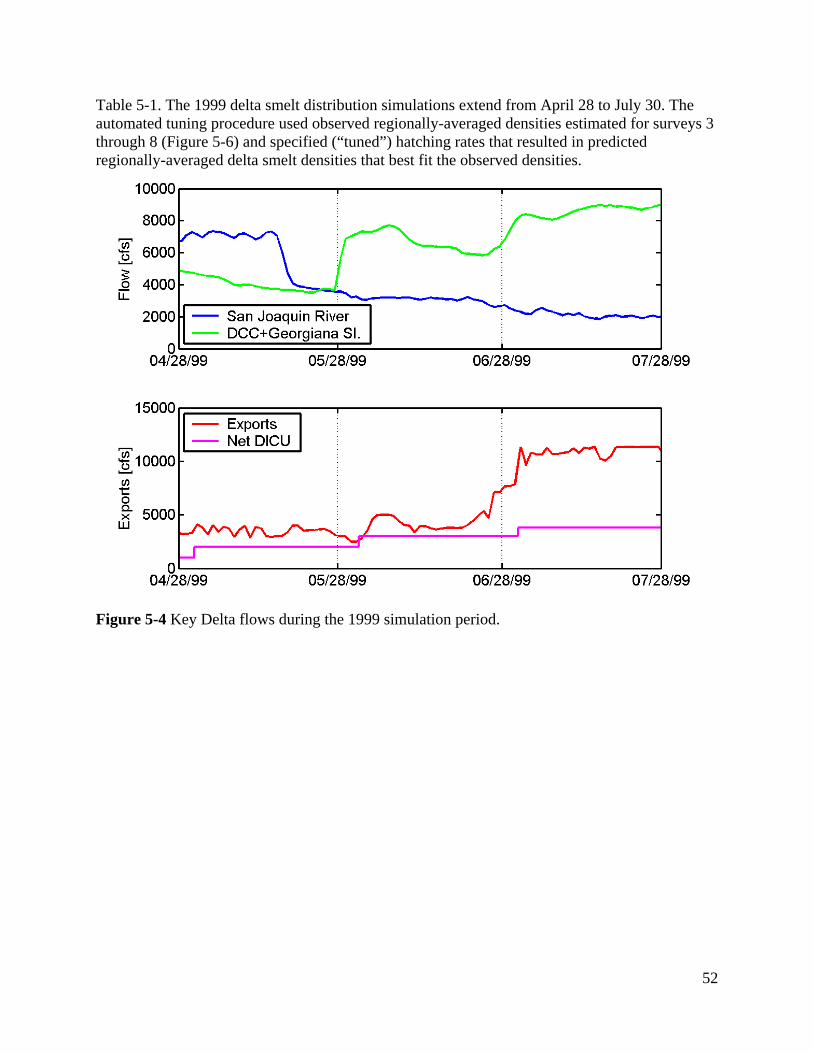
52

Table 5-1. The 1999 delta smelt distribution simulations extend from April 28 to July 30. The automated tuning procedure used observed regionally-averaged densities estimated for surveys 3 through 8 (Figure 5-6) and specified (“tuned”) hatching rates that resulted in predicted regionally-averaged delta smelt densities that best fit the observed densities.

Figure 5-4 Key Delta flows during the 1999 simulation period.

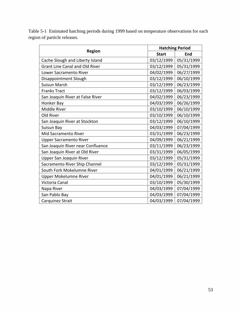
53

Table 5-1 Estimated hatching periods during 1999 based on temperature observations for each region of particle releases.

Region Hatching Period 

Start  End Cache Slough and Liberty Island  03/12/1999  05/31/1999Grant Line Canal and Old River  03/12/1999  05/31/1999Lower Sacramento River  04/02/1999  06/27/1999Disappointment Slough  03/12/1999  06/10/1999Suisun Marsh  03/12/1999  06/23/1999Franks Tract  03/12/1999  06/03/1999San Joaquin River at False River  04/02/1999  06/23/1999Honker Bay  04/03/1999  06/26/1999Middle River  03/10/1999  06/10/1999Old River  03/10/1999  06/10/1999San Joaquin River at Stockton  03/12/1999  06/10/1999Suisun Bay  04/03/1999  07/04/1999Mid Sacramento River  03/31/1999  06/23/1999Upper Sacramento River  04/09/1999  06/21/1999San Joaquin River near Confluence  03/11/1999  06/23/1999San Joaquin River at Old River  03/31/1999  06/05/1999Upper San Joaquin River  03/12/1999  05/31/1999Sacramento River Ship Channel  03/12/1999  05/31/1999South Fork Mokelumne River  04/01/1999  06/21/1999Upper Mokelumne River  04/01/1999  06/21/1999Victoria Canal  03/10/1999  05/30/1999Napa River  04/03/1999  07/04/1999San Pablo Bay  04/03/1999  07/04/1999Carquinez Strait  04/03/1999  07/04/1999

54

Figure 5-5 Regionally-averaged observed density of delta smelt (fish per 10,000 m3) in survey 2 of 1999.

Figure 5-6 Regionally-averaged observed density of delta smelt (fish per 10,000 m3) in surveys 2 through 8 of 1999.

55

5.2.1 Passive Scenario The hatching rates estimated by the automated tuning procedure (Figure 5-7) suggest that most of the hatching occurs in the western Delta and the central Delta. Non-zero hatching rates were estimated in ten regions, and the other regions were estimated to have no hatching. These results suggest that the automated tuning procedure tends to concentrate the hatching in small portion of the Delta. An artificial characteristic of the predicted hatching distribution is that the regions with largest predicted hatching border regions with no predicted hatching. This occurs because only the optimized hatching rates are provided by the Differential Evolution method. Because particles released in any one region are transported through the Delta, it may be difficult to distinguish the different effect of hatching in adjacent regions on delta smelt distribution. In reality, regional hatching rates seem likely to vary smoothly and hatching is likely to be occurring in many of the regions with no predicted hatching. A more robust method for estimating hatching distribution that should not suffer from this artifact of predicting no hatching in many regions will be discussed in Section 7.

The predicted delta smelt densities for surveys 3 (Figure 5-8) through 8 (Figure 5-13) match some patterns in the observed densities, resulting in a model skill score of 0.60, a high model skill score. Specifically, the highest delta smelt densities are typically observed in the western Delta and the distribution shifts seaward in the later surveys. In some regions, such as the Sacramento River Deep Water Ship Channel, no survey data was present (Figure 5-3). The majority of the delta smelt predicted to be present in the Delta for all the surveys result from hatching. In contrast, most of the fish that were present at the beginning of the simulation (on April 28th) are soon flushed from the Delta or lost as a result of natural mortality.

The predicted salvage of delta smelt at the (CVP) Tracy Fish Facility is compared with observed salvage in Figure 5-14. The magnitude and timing of salvage are predicted reasonably well. The predicted salvage results are sensitive to the initial release densities which are based upon 20-mm survey data from survey 2. Because 42 days are required for the simulated hatched fish to reach 20 mm length, the predicted hatching rates have a small effect on the predicted number of delta smelt that would be counted in salvage at the Tracy Fish Facility.

Figure 5-15 shows the observed regionally-averaged densities data for surveys 3 through 8 that was used in the optimization of hatching rates. Figure 5-16 shows the corresponding predicted regionally-averaged densities for surveys 3 through 8. Comparison of these two figures suggests that many of the spatial and temporal trends in regionally-averaged density are successfully predicted.

56

Figure 5-7 Estimated regional hatching rates in 1999 for the passive scenario.

Figure 5-8 Observed and predicted regionally-averaged delta smelt density (fish per 10,000 m3) in survey 3 of 1999 for the passive scenario.

57

Figure 5-9 Observed and predicted regionally-averaged delta smelt density (fish per 10,000 m3) in survey 4 of 1999 for the passive scenario.

Figure 5-10 Observed and predicted regionally-averaged delta smelt density (fish per 10,000 m3) in survey 5 of 1999 for the passive scenario.

58

Figure 5-11 Observed and predicted regionally-averaged delta smelt density (fish per 10,000 m3) in survey 6 of 1999 for the passive scenario.

Figure 5-12 Observed and predicted regionally-averaged delta smelt density (fish per 10,000 m3) in survey 7 of 1999 for the passive scenario.

59

Figure 5-13 Observed and predicted regionally-averaged delta smelt density (fish per 10,000 m3) in survey 8 of 1999 for the passive scenario.

Figure 5-14 Observed and predicted daily salvage at the Tracy Fish Facility in 1999 for the passive scenario.

60

Figure 5-15 Regionally-averaged observed density of delta smelt (fish per 10,000 m3) in surveys 3 through 8 of 1999.

Figure 5-16 Regionally-averaged predicted density of delta smelt (fish per 10,000 m3) in surveys 3 through 8 of 1999 for the passive scenario.

61

5.2.2 Steady Upward Swimming Scenario The 1999 delta smelt distribution simulation was repeated with the addition of a steady upward migration behavior. This “swimming” behavior can be achieved by a combination of buoyancy provided by a swim bladder and active swimming. The swimming behavior was chosen to be consistent with observations of vertical distribution (e.g. Bennet et al., 2002; Hobbs et al., 2006). The swimming speed is steady in time and varies with vertical position from a speed of 1 mm s-1 upward swimming at depths below 6 meters depth and no swimming at 2 meters from the surface. The effect of the vertical swimming behavior is an increase in the delta smelt density high in the water column and a decrease in delta smelt density low in the water column.

The hatching rates estimated by the automated tuning procedure (Figure 5-17) suggests that most of the hatching occurs in the western Delta and the central Delta. Non-zero hatching rates were estimated in twelve regions, and the other regions were estimated to have no hatching. Non-zero hatching rates were predicted in only ten regions for the passive particle simulation. Two key differences in the hatching distribution are increased hatching rates and the presence of hatching in the Sacramento River Deep Water Ship Channel for the steady upward swimming scenario. This occurs because the upward swimming particles/fish tend to exit the Delta sooner than the passive particles. Therefore, in order to compensate for this faster exit from the Delta, and match the fish densities that were observed in the western Delta in the later surveys, after the hatching period has ended, additional hatching is required and the hatching distribution must shift landward, relative to the hatching distribution predicted for the passive scenario. Otherwise the hatching distribution is similar to the hatching distribution predicted for the passive scenario. The model skill score for the steady upward swimming scenario is 0.63, compared with a model skill score of 0.60 for the passive scenario. Therefore, this simple hypothesized behavior does not appear to provide a substantial improvement in the predictive power of the simulation. The prediction of hatching in the Sacramento is consistent with delta smelt observations in that region (Grimaldo, personal communication) which may suggest that the hatching distribution for this scenario may be more realistic than the hatching distribution for the passive scenario.

The predicted delta smelt densities for surveys 3 through 8 (Figure 5-18 through Figure 5-23) match some patterns in the observed densities. Specifically, the highest delta smelt densities are typically observed in the western Delta and the distribution shifts seaward in the later surveys. The majority of the delta smelt predicted to be present in the Delta for all the surveys result from hatching. In contrast, most of the fish that were present at the beginning of the simulation (on April 28th) are soon flushed from the Delta or lost as a result of natural mortality.

The predicted salvage of delta smelt at the (CVP) Tracy Fish Facility is compared with observed salvage in Figure 5-24. The magnitude and timing of salvage are predicted reasonably well. The predicted salvage results are sensitive to the initial release densities which are based upon sampling data for survey 2. Because 42 days are required for the simulated hatched fish to reach 20 mm length, the predicted hatching rates have a small effect on the predicted number of delta smelt that would be counted in salvage at the Tracy Fish Facility.

Figure 5-25 shows the observed regionally-averaged densities data for surveys 3 through 8 that was used in the optimization of hatching rates. Figure 5-26shows the corresponding predicted regionally-averaged densities for surveys 3 through 8. Comparison of these two figures suggests

62

that many of the spatial and temporal trends in regionally-averaged density are successfully predicted.

Figure 5-17 Estimated regional hatching rates in 1999 for the steady upward swimming scenario.

63

Figure 5-18 Observed and predicted regionally-averaged delta smelt density (fish per 10,000 m3) in survey 3 of 1999 for the steady upward swimming scenario.

Figure 5-19 Observed and predicted regionally-averaged delta smelt density (fish per 10,000 m3) in survey 4 of 1999 for the steady upward swimming scenario.

64

Figure 5-20 Observed and predicted regionally-averaged delta smelt density (fish per 10,000 m3) in survey 5 of 1999 for the steady upward swimming scenario.

Figure 5-21 Observed and predicted regionally-averaged delta smelt density (fish per 10,000 m3) in survey 6 of 1999 for the steady upward swimming scenario.

65

Figure 5-22 Observed and predicted regionally-averaged delta smelt density (fish per 10,000 m3) in survey 7 of 1999 for the steady upward swimming scenario.

Figure 5-23 Observed and predicted regionally-averaged delta smelt density (fish per 10,000 m3) in survey 8 of 1999 for the steady upward swimming scenario.

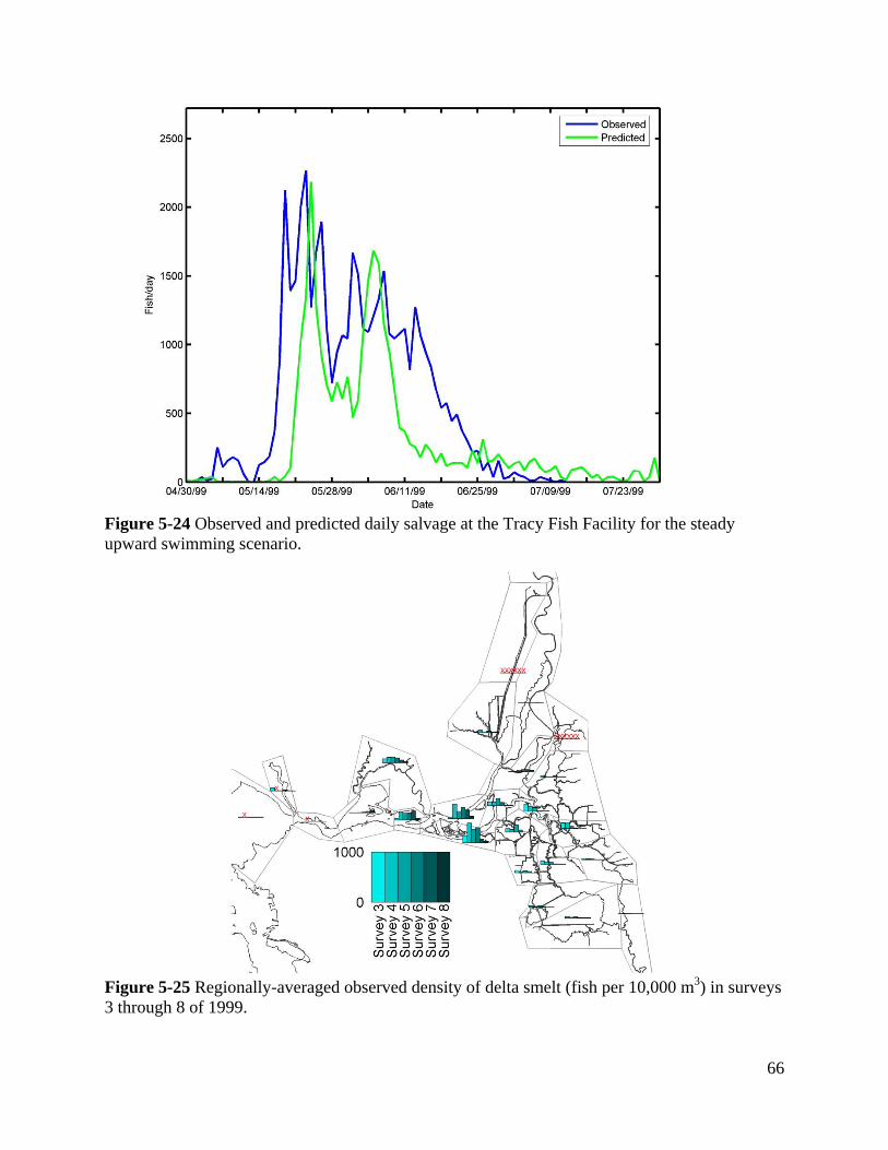
66

Figure 5-24 Observed and predicted daily salvage at the Tracy Fish Facility for the steady upward swimming scenario.

Figure 5-25 Regionally-averaged observed density of delta smelt (fish per 10,000 m3) in surveys 3 through 8 of 1999.

67

Figure 5-26 Regionally-averaged predicted density of delta smelt (fish per 10,000 m3) in surveys 3 through 8 of 1999 for the steady upward swimming scenario.

5.2.3 Diurnal Upward Swimming Scenario The 1999 delta smelt distribution simulation was repeated with the addition of a diurnal upward swimming behavior. The specified behavior used the same speeds and vertical distribution as the steady upward swimming behavior scenario. Specifically, before 6 AM the particles were specified to be passive. Between 6 AM and 7 AM, the vertical swimming behavior is phased in (“ramped up”) linearly. The behavior is specified until 6 PM and then phased out from 6 PM to 7 PM. So the behavior roughly corresponds to upward swimming during daylight hours and passive behavior during nighttime hours.

The hatching rates estimated by the automated tuning procedure (Figure 5-27) suggest that most of the hatching occurs in the western Delta and central Delta. Non-zero hatching rates were estimated in 12 regions, and the other regions were estimated to have no hatching. The patterns of predicted hatching are very similar for the diurnal upward swimming scenario and the steady upward swimming scenario. The model skill score for the steady upward swimming scenario is 0.62, compared with a model skill score of 0.63 for steady upward swimming and 0.60 for the passive scenario. Therefore, diurnal upward swimming does not appear to provide an improvement in the predictive power of the simulation relative to steady upward swimming.

The predicted delta smelt densities for surveys 3 through 8 (Figure 5-28 through Figure 5-33) match some patterns in the observed densities. Specifically, the highest delta smelt densities are typically observed in the western Delta and the distribution shifts seaward in the later surveys. The majority of the delta smelt predicted to be present in the Delta for all the surveys result from hatching. In contrast, most of the fish that were present at the beginning of the simulation (on April 28th) are soon flushed from the Delta or lost as a result of natural mortality.

68

The predicted salvage of delta smelt at the (CVP) Tracy Fish Facility is compared with observed salvage in Figure 5-34. The magnitude and timing of salvage are predicted reasonably well. The predicted salvage results are sensitive to the initial release densities which are based upon sampling data for survey 2. Because 42 days are required for the simulated hatched fish to reach 20 mm length, the predicted hatching rates have a small effect on the predicted number of delta smelt that would be counted in salvage at the Tracy Fish Facility.

Figure 5-35 shows the observed regionally-averaged densities data for surveys 3 through 8 that was used in the optimization of hatching rates. Figure 5-36 shows the corresponding predicted regionally-averaged densities for surveys 3 through 8. Comparison of these two figures suggests that many of the spatial and temporal trends in regionally-averaged density are successfully predicted.

Figure 5-27 Estimated regional hatching rates in 1999 for the diurnal upward swimming scenario.

69

Figure 5-28 Observed and predicted regionally-averaged delta smelt density (fish per 10,000 m3) in survey 3 of 1999 for the diurnal upward swimming scenario.

70

Figure 5-29 Observed and predicted regionally-averaged delta smelt density (fish per 10,000 m3) in survey 4 of 1999 for the diurnal upward swimming scenario.

Figure 5-30 Observed and predicted regionally-averaged delta smelt density (fish per 10,000 m3) in survey 5 of 1999 for the diurnal upward swimming scenario.

71

Figure 5-31 Observed and predicted regionally-averaged delta smelt density (fish per 10,000 m3) in survey 6 of 1999 for the diurnal upward swimming scenario.

Figure 5-32 Observed and predicted regionally-averaged delta smelt density (fish per 10,000 m3) in survey 7 of 1999 for the diurnal upward swimming scenario.

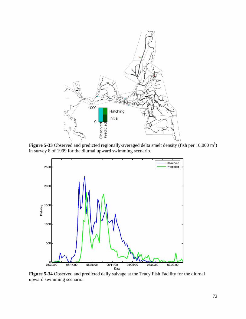
72

Figure 5-33 Observed and predicted regionally-averaged delta smelt density (fish per 10,000 m3) in survey 8 of 1999 for the diurnal upward swimming scenario.

Figure 5-34 Observed and predicted daily salvage at the Tracy Fish Facility for the diurnal upward swimming scenario.

73

Figure 5-35 Regionally-averaged observed density of delta smelt (fish per 10,000 m3) in surveys 3 through 8 of 1999.

Figure 5-36 Regionally-averaged predicted density of delta smelt (fish per 10,000 m3) in surveys 3 through 8 of 1999 for the diurnal upward swimming scenario.

74

5.2.4 Life Stage Dependent Diurnal Upward Swimming Scenario The 1999 delta smelt distribution simulation was repeated with the addition of a diurnal upward swimming behavior which begins 40 days after particle hatching, roughly corresponding to 19 mm fork length of delta smelt, a length at which swim bladders become functional (Mager et al., 2004). The initially released fish (specified based on the delta smelt distribution observed in survey 2) are all assumed to be greater than 19 mm long and, therefore, have the diurnal swimming behavior for the entire simulation period. The specified behavior used the same speeds, vertical distribution and diurnal variability as the diurnal upward swimming behavior scenario.

The hatching rates estimated by the automated tuning procedure (Figure 5-37) suggest that most of the hatching occurs in the western Delta and central Delta. Non-zero hatching rates were estimated in nine regions, and the other regions were estimated to have no hatching. The patterns of predicted hatching were very similar for the passive scenario and the life stage dependent diurnal upward swimming scenario. The model skill score for the life stage dependent diurnal upward swimming scenario is 0.60, the same as the passive scenario. Therefore, this simple hypothesized behavior does not appear to provide an improvement in the predictive power of the simulation relative to the passive scenario.

The predicted delta smelt densities for surveys 3 through 8 (Figure 5-38 through Figure 5-43) match some patterns in the observed densities. Specifically, the highest delta smelt densities are typically observed in the western Delta and the distribution shifts seaward in the later surveys. Note that the majority of the delta smelt predicted to be present in the Delta for all the surveys result from hatching. In contrast, most of the fish that were present at the beginning of the simulation (on April 28th) are soon flushed from the Delta or lost as a result of natural mortality.

The predicted salvage of delta smelt at the (CVP) Tracy Fish Facility is compared with observed salvage in Figure 5-44. The magnitude and timing of salvage are predicted reasonably well. The predicted salvage results are sensitive to the initial release densities which are based upon sampling data for survey 2. Because 42 days are required for the simulated hatched fish to reach 20 mm length, the predicted hatching rates have a small effect on the predicted number of delta smelt that would be counted in salvage at the Tracy Fish Facility.

Figure 5-45 shows the observed regionally-averaged densities data for surveys 3 through 8 that was used in the optimization of hatching rates. Figure 5-46 shows the corresponding predicted regionally-averaged densities for surveys 3 through 8. Comparison of these two figures suggests that many of the spatial and temporal trends in regionally-averaged density are successfully predicted

75

Figure 5-37 Estimated regional hatching rates in 1999 for the diurnal upward swimming starting 40 days after hatching scenario.

Figure 5-38 Observed and predicted regionally-averaged delta smelt density (fish per 10,000 m3) in survey 3 of 1999 for the diurnal upward swimming starting 40 days after hatching scenario.

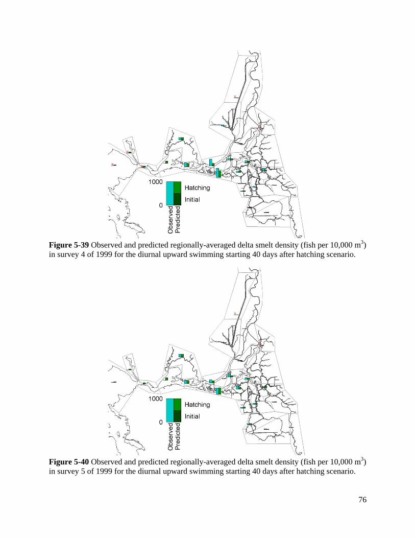
76

Figure 5-39 Observed and predicted regionally-averaged delta smelt density (fish per 10,000 m3) in survey 4 of 1999 for the diurnal upward swimming starting 40 days after hatching scenario.

Figure 5-40 Observed and predicted regionally-averaged delta smelt density (fish per 10,000 m3) in survey 5 of 1999 for the diurnal upward swimming starting 40 days after hatching scenario.

77

Figure 5-41 Observed and predicted regionally averaged delta smelt density (fish per 10,000 m3) in survey 6 of 1999 for the diurnal upward swimming starting 40 days after hatching scenario.

Figure 5-42 Observed and predicted regionally-averaged delta smelt density (fish per 10,000 m3) in survey 7 of 1999 for the diurnal upward swimming starting 40 days after hatching scenario.

78

Figure 5-43 Observed and predicted regionally-averaged delta smelt density (fish per 10,000 m3) in survey 8 of 1999 for the diurnal upward swimming starting 40 days after hatching scenario.

Figure 5-44 Observed and predicted daily salvage at the Tracy Fish Facility for the diurnal upward swimming starting 40 days after hatching scenario.

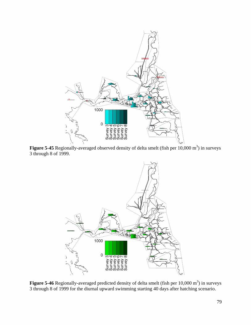
79

Figure 5-45 Regionally-averaged observed density of delta smelt (fish per 10,000 m3) in surveys 3 through 8 of 1999.

Figure 5-46 Regionally-averaged predicted density of delta smelt (fish per 10,000 m3) in surveys 3 through 8 of 1999 for the diurnal upward swimming starting 40 days after hatching scenario.

80

5.2.5 Comparison of Scenarios The hatching distributions for the different behavior scenarios are compared in Figure 5-47. Some differences in hatching rates are notable but the overall predicted patterns of hatching are similar for all of the scenarios. Therefore, for juvenile delta smelt simulations it may be adequate to represent the delta smelt with passive particles.

Figure 5-47 Estimated hatching distributions for different behavior scenarios.

5.3 2007 Hatching Distribution Simulation The 20-mm survey period during 2007 was chosen as a simulation period representative of recent years with low abundance of delta smelt. Because the estimated hatching distributions were fairly similar among the different behavior scenarios for 1999, only the passive behavior scenario is simulated for 2007. Key flows during the 2007 simulation period are shown in Figure 5-48 The initial density of delta smelt in the estuary was specified using a survey corresponding to the starting time of the simulation. For 2007, survey 3 observations were used (Figure 5-49). The

81

particles representing the initial distribution of delta smelt were released at an hourly interval for 24 hours starting at 12:00 am on April 11, 2007.

The hatching periods are specified for each of the regions based on temperature observations for 2007, using the approach described in Section 5.1. The hatching periods are reported in Table 5-2.

The 2007 delta smelt distribution simulations extend from April 11 to July 4, allowing the automated tuning procedure to use observations for surveys 4 through 9 (Figure 5-50). It should be noted that the observed regionally-averaged delta smelt density (Figure 5-50) shows minimal spatial or temporal coherence. Instead there appears to be a large “random” component in the regional delta smelt density that appears due to the very small and intermittent number of fish caught in 20-mm trawls during 2007. This makes 2007 a much more difficult period than 1999 for estimation of delta smelt hatching distribution.

Figure 5-48 Key Delta flows during the 2007 simulation period.

82

Table 5-2 Estimated hatching periods during 2007 based on temperature observations for each region of particle releases.

Region Hatching Period 

Start  End Cache Slough and Liberty Island  2/11/2007 5/10/2007 Grant Line Canal and Old River  2/12/2007 5/02/2007 Lower Sacramento River  3/12/2007 6/15/2007 Disappointment Slough  2/15/2007 5/02/2007 Suisun Marsh  2/12/2007 6/26/2007 Franks Tract  2/20/2007 5/12/2007 San Joaquin River at False River  3/09/2007 6/12/2007 Honker Bay  3/11/2007 6/15/2007 Middle River  2/20/2007 5/11/2007 Old River  2/20/2007 5/11/2007 San Joaquin River at Stockton  2/15/2007 5/02/2007 Suisun Bay  2/20/2007 6/26/2007 Mid Sacramento River  2/17/2007 5/26/2007 Upper Sacramento River  3/10/2007 5/02/2007 San Joaquin River near Confluence  2/17/2007 5/25/2007 San Joaquin River at Old River  3/11/2007 5/24/2007 Upper San Joaquin River  2/12/2007 5/28/2007 Sacramento River Ship Channel  2/11/2007 5/10/2007 South Fork Mokelumne River  3/11/2007 6/26/2007 Upper Mokelumne River  3/11/2007 6/26/2007 Victoria Canal  2/19/2007 5/11/2007 Napa River  2/20/2007 6/26/2007 San Pablo Bay  2/20/2007 6/26/2007 Carquinez Strait  2/20/2007 6/26/2007

83

Figure 5-49 Regionally-averaged observed density of delta smelt (fish per 10,000 m3) in survey 3 of 2007.

Figure 5-50 Regionally-averaged observed density of delta smelt (fish per 10,000 m3) in surveys 4 through 9 of 2007.

84

5.3.1 Passive Scenario The automated tuning procedure (Figure 5-51) estimated that all of hatching occurs in 4 regions. All other regions were estimated to have no hatching.

The predicted delta smelt densities for surveys 4 (Figure 5-52) through 8 (Figure 5-57) do not match the observed densities closely. This is not surprising, because the observed densities themselves (Figure 5-50) show minimal spatial or temporal coherence. The only clear trend visible in the observations, namely the location of most peak observed densities in the western Delta, is also predicted. The majority of the delta smelt predicted to be present in the Delta for all the surveys result from hatching.

The predicted salvage of delta smelt at the (CVP) Tracy Fish Facility is compared with observed salvage in Figure 5-58. The observed salvage is quite low and, for that reason, “noisy,” so it is not clear whether the salvage is predicted well. The order of magnitude of predicted salvage is similar to the order of magnitude of observed salvage. The predicted salvage results are sensitive to the initial release densities which are based upon 20-mm survey data from survey 3. Because 42 days are required for the simulated hatched fish to reach 20 mm length, the predicted hatching rates have a small effect on the predicted number of delta smelt that would be counted in salvage at the Tracy Fish Facility. Figure 5-49 shows the observed regionally-averaged densities data for surveys 4 through 8 that was used in the optimization of hatching rates. Figure 5-50 shows the corresponding predicted regionally-averaged densities for surveys 4 through 8. Comparison of these two figures suggests that many of the spatial and temporal trends in regionally-averaged density are successfully predicted

The model skill for the 2007 delta smelt distribution simulation was 0.014, compared with a model skill of 0.60 for the 1999 passive scenario. This low model skill, which suggests minimal confidence in the predicted hatching distribution, was expected due to the large and “noisy” spatial and temporal variability in observed delta smelt density.

85

Figure 5-51 Estimated regional hatching rates in 2007 for the passive scenario.

Figure 5-52 Observed and predicted regionally-averaged delta smelt density (fish per 10,000 m3) in survey 4 of 2007 for the passive scenario.

86

Figure 5-53 Observed and predicted regionally-averaged delta smelt density (fish per 10,000 m3) in survey 5 of 2007 for the passive scenario.

Figure 5-54 Observed and predicted regionally-averaged delta smelt density (fish per 10,000 m3) in survey 6 of 2007 for the passive scenario.

87

Figure 5-55 Observed and predicted regionally-averaged delta smelt density (fish per 10,000 m3) in survey 7 of 2007 for the passive scenario.

Figure 5-56 Observed and predicted regionally-averaged delta smelt density (fish per 10,000 m3) in survey 8 of 2007 for the passive scenario.

88

Figure 5-57 Observed and predicted regionally-averaged delta smelt density (fish per 10,000 m3) in survey 9 of 2007 for the passive scenario.

Figure 5-58 Observed and predicted daily salvage at the Tracy Fish Facility in 2007 for the passive scenario.

89

Figure 5-59 Regionally-averaged observed density of delta smelt (fish per 10,000 m3) in surveys 4 through 9 of 2007.

Figure 5-60 Regionally-averaged predicted density of delta smelt (fish per 10,000 m3) in surveys 4 through 9 of 2007 for the passive scenario.

90

5.4 Possible Improvements to Delta Smelt Distribution Simulation Approach The delta smelt simulation approach documented here shows some success in predicting delta smelt distribution. Key simplifications inherent in the approach include the use of hatching rates which are constant through the hatching period in each region and a mortality rate that is both steady in time and uniform spatially. Possible improvements include estimation of variability of hatching throughout the hatching period and mortality dependent on life stage, location or other environmental factors. In many of the 1999 scenario results, the delta smelt densities were underestimated in later surveys. This suggests that the predicted hatching stopped too early. Therefore, it may be possible to improve predictions by refining the estimates of hatching periods.

Several additional improvements in the representation of delta smelt can be envisioned. However, because the hatching rates are estimated by “tuning” to match observed distributions, a substantial limitation on the predictive ability of the model is the limited accuracy of the estimated “observed” regionally-averaged densities that are derived from 20-mm survey observations. Enhancements of the method that would require addition of more tuned parameters might not be successful, because the available observations might not support confident specification of additional parameters.

Given the large uncertainties associated with sampling and forecasting delta smelt distribution, developing a useful delta smelt distribution prediction methodology for recent conditions of low observed delta smelt density requires quantification of uncertainty. An appropriate approach would allow hatching rates, delta smelt distribution, and entrainment estimates to be reported in terms of confidence intervals. For example, the approach may estimate a 90% confidence that the hatching rate in the Lower Sacramento River region for a given period was between 0.010 fish m-2 day-1 and 0.022 fish m-2 day-1. Similarly, the approach may estimate that 180 or fewer fish would be entrained in two weeks at a 50% confidence interval and 520 or fewer fish would be entrained in two weeks at a 90% confidence interval. Using a probabilistic approach and reporting confidence intervals and other probabilistic information would greatly increase the value of the predictions relative to a single “best guess” of delta smelt hatching, distribution and entrainment. The suggested methodology to address uncertainty is Bayesian inference with Markov chain Monte Carlo sampling. This is a widely used methodology that is currently applied in diverse applications, some of which are similar to the proposed delta smelt applications. An existing Bayesian inference approach and code (e.g., Delle Monache et al., 2008) could be modified and applied to the delta smelt simulations. The integration of the Bayesian inference approach into the analysis software would follow a similar structure as the current integration of the Differential Evolution algorithm (Price and Storn, 1998) into the existing analysis software and methodology. These two well-established analysis methods have several aspects in common, most notably the use of specified error metrics (“likelihood function” in Bayesian inference terminology) and similar methods for sampling the parameter space.

5.5 Summary of Delta Smelt Distribution Simulation Results 

91

The delta smelt modeling approach applied in this study provides an objective method to estimate hatching distributions using modeling tools and observations. The hatching distributions predicted indicate hatching in areas that are consistent with current biological understanding based on larval surveys and 20-mm observations. However, the approach also concentrates hatching in a limited number of regions, and, therefore, is likely to underestimate the spatial extent of hatching. The comparisons with observed distributions of larval and juvenile delta smelt show some similarities and some differences. Given the large variability in observed regionally-averaged densities from survey to survey and region to region, the differences between observed and predicted regionally-averaged densities were expected. The estimated fates of the population of larval and juvenile delta smelt in 1999 are presented in Table 5-3. This table shows that many more fish were hatched after survey 2 than were present at the time of the beginning of the simulations (corresponding to survey 2). The fate of most of the larval and juvenile delta smelt is loss from natural mortality. The estimated entrainment losses for the different scenarios correspond to 2% to 3% of the total larval and juvenile fish which are estimated to hatch during 1999. In all scenarios, less than 20% of the fish hatched during 1999 are estimated to survive to the end of the simulation on July 21, 1999 corresponding to the end of the 20-mm survey period (survey 8). Table 5-3 Estimated fates of the larval and juvenile delta smelt in 1999.

Category  Passive  Steady  Diurnal 40 daysHatched  59.02  67.53  66.06 59.36Initial  12.20  12.20  12.20 12.20Alive  10.80  14.55  13.80 11.67

Entrained  1.31  1.10  1.12 1.33Diversions  0.74  0.74  0.76 0.77Mortality  58.38  63.35  62.58 57.80

Table 5-3 does not provide enough information to estimate the percent loss of delta smelt associated with entrainment by water exports during the simulation period. We estimate % loss of delta smelt as the number of additional delta smelt that would have been present at the time of survey 8 if entrainment had not occurred divided by the total number of delta smelt alive at the time of survey 8. Note that the number of additional delta smelt that would have been present at the time of survey 8 is much smaller than the total number entrained because most of the delta smelt entrained would have been lost to natural mortality processes before the time of survey 8 had they not been entrained. The estimated percent loss is 3.2% for the passive scenario, 2.0% for the steady behavior scenario, 2.1% for the diurnal behavior scenario and 2.7% for the diurnal behavior at 40 days scenario. The annual percent loss reported in Kimmerer (2009) is approximately 8% for 1999, with quite large estimated error bounds. Our estimates of 2% to 3% are substantially smaller but note that we do not refer to these as annual % loss because there is a substantial difference between the meaning of the Kimmerer (2009) estimate and the numbers reported here. The percent loss reported here accounts for losses starting at survey 2 (April 28, 1999, corresponding to the beginning of the particle tracking simulation), while the annual percent loss estimated by

92

Kimmerer (2009) includes entrainment losses starting at the time of the first estimated hatch date (March 21, 1999). This may account for a substantial portion of the differences between the estimated losses because the daily proportional losses estimated by Kimmerer (2009) are largest in early April. There are also differences in the estimated end of hatching. The hatching periods used in this study varied regionally (Table 5-1) and, in regions with large hatching rates, such as the San Joaquin River near the Confluence, the hatching period extended two weeks beyond the estimated end of hatching in Kimmerer (2009) of June 9, 1999. The last cohorts are much more likely to survive to survey 8 than the early cohorts, so this difference would also tend to make our estimated percent loss smaller than that estimated by Kimmerer (2009).

There are also many differences between the approach used here and the approach of Kimmerer (2009). The most obvious difference is that the Kimmerer approach could be considered a “box model” while the approach reported here uses high resolution hydrodynamics and spatially explicit particle tracking. A specific example is that the density of fish in the south delta is calculated by Kimmerer using an averaged of the observed density at six stations in the south delta. Instead, the approach used here tracks particles/fish directly to the entrainment locations and, therefore does not directly use spatial averaging to estimate entrainment losses. The estimated “total population” of delta smelt are also different between the approaches because regional abundances are estimated from the 20-mm survey data (see Figure 5-3) and summed together in our approach whereas Kimmerer (2009) estimates an average density within the region of delta smelt habitat from the 20-mm survey data and multiplies by the volume of habitat of delta smelt. The hatching distributions estimated for simulations with different hypothesized vertical migration behaviors are similar to the hatching distributions estimated for passive particle tracking scenario. The resulting estimated values of percent loss to export pumping of the overall population of larval and juvenile delta smelt are also similar among scenarios. Furthermore, the inclusion of behavior in the particle tracking scenarios does not result in substantially improved comparison with observed delta smelt densities. Therefore we conclude that the vertical migration behaviors explored so far have limited influence on delta smelt distribution and fate. A natural next step in the modeling approach is extension to providing probabilistic predictions. Given the large uncertainties in estimating delta smelt distribution and entrainment from observations, modeling approaches to predict distribution or entrainment that do not explicitly estimate the uncertainty in model predictions could be highly misleading. The estimates of delta smelt distribution and, in particular, hatching distribution, are extremely relevant to ongoing policy decisions. Any project that modifies flow pathways and mixing in the Delta is likely to decrease entrainment of fish from some regions and increase entrainment of fish from other regions. Therefore, in order to confidently estimate impacts of such project, it is critical to estimate the distribution of delta smelt and any other relevant fish species. Modeling tools and approaches such as the one described in this section, particularly if applied in a probabilistic framework, will be useful supplements to ongoing observational programs in estimating the distribution and entrainment of delta smelt and other species for current conditions and different Delta operations scenarios.

93

6 Particle Fate Simulations In this section, the fate of particles released in different regions is estimated for different simulation periods and different vertical migration behaviors. These fate estimates have some similarities and some differences with respect to the intermodel comparison simulations. As in the intermodel comparisons, particles are released over a 24 hour period on a specified release date and fates are reported two months after particle release. Several differences from the intermodel comparison simulations are notable. First of all the particles are released regionally, as opposed to releases at specific stations. This is a substantial advantage, because, as discussed in Section 4, particle fate is highly sensitive to exact release location. Therefore, the fate of releases at some station locations may be misleading because they are not representative of “typical conditions” in a region. Second, the entrainment in agricultural diversions is estimated, as discussed in Section 5. The possible “final” fates for each particle are entrainment by export facilities including the SWP, the SCP, the North Bay Aqueduct and the CCWD exports, entrainment by agricultural diversions, and exit past a line in Martinez that corresponds to the boundary of the DSM2 model, reported as “exited Delta.” Particles that are still present at the end of the simulations have not yet reached these final fates and are reported as “within Delta.” In addition, natural mortality is also estimated, using a mortality rate of 0.05 day-1, corresponding roughly to the value used for juvenile delta smelt in 1999 by Kimmerer (2008), as was used in the hatching distribution simulations. The probability of the particle being “alive” decreases exponentially in time. Specifically, if one particle initially represents 1 live fish then after 13.9 days the particle would represent 0.5 live fish, and the other 0.5 fish is estimated to be lost due to natural mortality. Therefore entrainment of a particle early in the simulation period contributes more to the count of entrained “fish” than the entrainment of a particle late in the entrainment period.

6.1 April 28, 1999 Passive Particle Scenario   Fate was estimated for particle releases on April 28, 1999. This particle release time was also used for intermodel comparisons in Section 4. However, as discussed above, the scenarios discussed in this section used regional releases instead of the point releases used in the intermodel comparisons. Figure 6-1 shows the fates of passive particles released on April 28, 1999 after 60 days of simulation. As expected, entrainment increases with proximity to the water exports and the gradients in entrainment are quite sharp in the central Delta. A substantial portion of the particles are estimated to be entrained by agricultural diversions. When natural mortality is considered, it is the dominant fate at most locations. However, inclusion of natural mortality has a smaller effect on the proportion of particles that are entrained in the far south Delta (e.g. in Grant Line Canal) due to the relatively short transit time to the export pumps for particles released in the far south Delta.

94

Figure 6-1 Fates of passive particles released on April 28, 1999 and tracked for 60 days. (A) Fates without natural mortality; (B) Fates with natural mortality.

6.2 April 28, 1999 Steady Upward Swimming Scenario   Figure 6-2 shows the fates of steady upward swimming particles released on April 28, 1999 after 60 days of simulation. As expected, entrainment increases with proximity to the water exports and the gradients in entrainment are quite sharp in the central Delta. A substantial portion of the particles were estimated to be entrained by agricultural diversions. When natural mortality is considered, it is the dominant fate at most locations. However, inclusion of natural mortality has a smaller effect on the proportion of particles that are entrained in the far south Delta (e.g. in Grant Line Canal) due to the relatively short transit time to the export pumps for particles released in the far south Delta.

95

Figure 6-2 Fates of constant upward swimming particles released on April 28, 1999 and tracked for 60 days. (A) Fates without natural mortality; (B) Fates with natural mortality.

6.3 April 28, 1999 Diurnal Upward Swimming Scenario   Figure 6-3 shows the fates of diurnal upward swimming particles released on April 28, 1999 after 60 days of simulation. As expected, entrainment increases with proximity to the water exports and the gradients in entrainment are quite sharp in the central Delta. A substantial portion of the particles were estimated to be entrained by agricultural diversions. When natural mortality is considered, it is the dominant fate at most locations. However, inclusion of natural mortality has a smaller effect on the proportion of particles that are entrained in the far south Delta (e.g. in Grant Line Canal) due to the relatively short transit time to the export pumps for particles released in the far south Delta.

96

Figure 6-3 Fates of diurnal upward swimming particles released on April 28, 1999 and tracked for 60 days. (A) Fates without natural mortality; (B) Fates with natural mortality.

6.4 April 28, 1999 Diurnal Upward Swimming at 40 Days Scenario   Figure 6-4 shows the fates of particles for the diurnal upward swimming at 40 days scenario with particles released on April 28, 1999. The fates are reported after 60 days of simulation. As expected, entrainment increases with proximity to the water exports and the gradients in entrainment are quite sharp in the central Delta. A substantial portion of the particles were estimated to be entrained by agricultural diversions. When natural mortality is considered, it is the dominant fate at most locations. However, inclusion of natural mortality has a smaller effect on the proportion of particles that are entrained in the far south Delta (e.g. in Grant Line Canal) due to the relatively short transit time to the export pumps for particles released in the far south Delta.

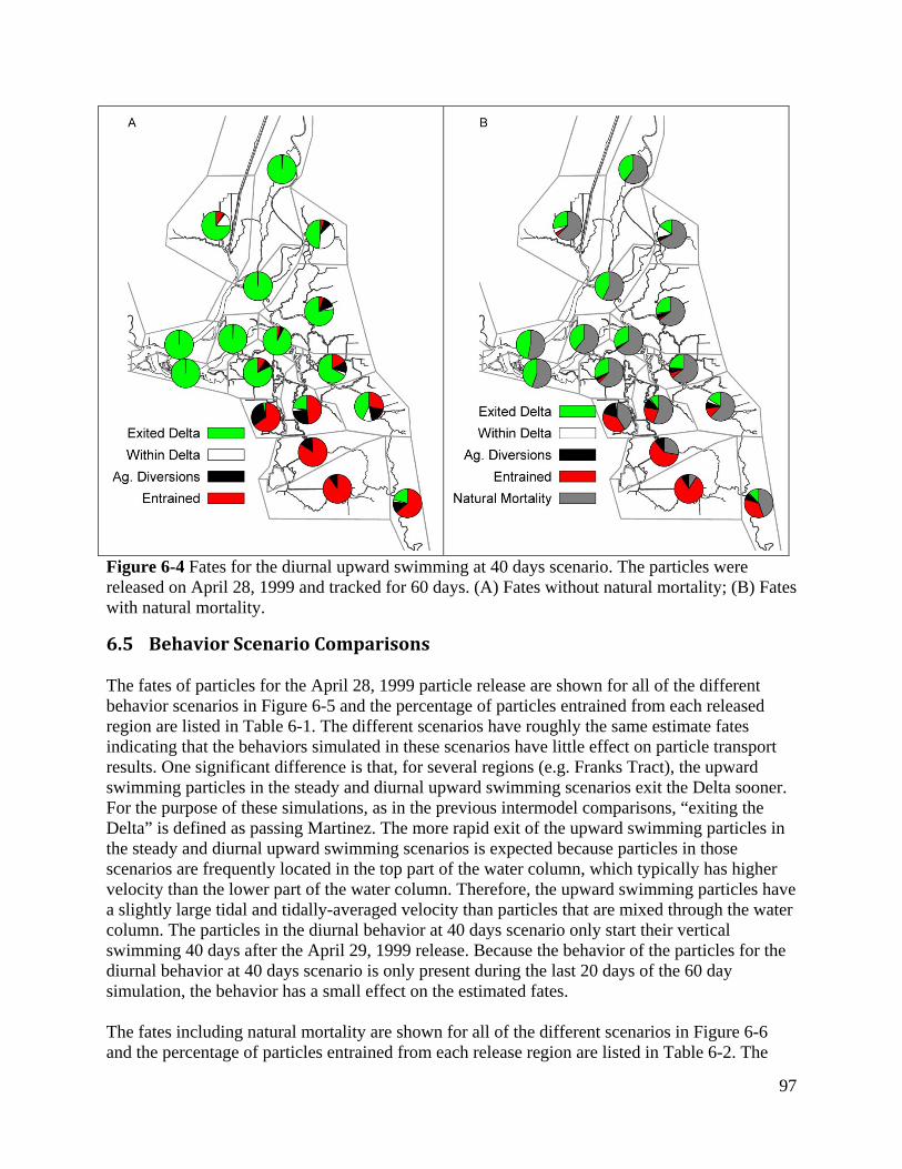
97

Figure 6-4 Fates for the diurnal upward swimming at 40 days scenario. The particles were released on April 28, 1999 and tracked for 60 days. (A) Fates without natural mortality; (B) Fates with natural mortality.

6.5 Behavior Scenario Comparisons  The fates of particles for the April 28, 1999 particle release are shown for all of the different behavior scenarios in Figure 6-5 and the percentage of particles entrained from each released region are listed in Table 6-1. The different scenarios have roughly the same estimate fates indicating that the behaviors simulated in these scenarios have little effect on particle transport results. One significant difference is that, for several regions (e.g. Franks Tract), the upward swimming particles in the steady and diurnal upward swimming scenarios exit the Delta sooner. For the purpose of these simulations, as in the previous intermodel comparisons, “exiting the Delta” is defined as passing Martinez. The more rapid exit of the upward swimming particles in the steady and diurnal upward swimming scenarios is expected because particles in those scenarios are frequently located in the top part of the water column, which typically has higher velocity than the lower part of the water column. Therefore, the upward swimming particles have a slightly large tidal and tidally-averaged velocity than particles that are mixed through the water column. The particles in the diurnal behavior at 40 days scenario only start their vertical swimming 40 days after the April 29, 1999 release. Because the behavior of the particles for the diurnal behavior at 40 days scenario is only present during the last 20 days of the 60 day simulation, the behavior has a small effect on the estimated fates. The fates including natural mortality are shown for all of the different scenarios in Figure 6-6 and the percentage of particles entrained from each release region are listed in Table 6-2. The

98

natural mortality in some regions is slightly lower for the steady upward and diurnal upward swimming scenarios. This is expected because, as previously noted, the particles for these scenarios exit the Delta sooner, and the natural mortality is estimated during the time required for the particles to reach a “final” fate, such as exit from the Delta. Table 6-1 Estimated entrainment of particles for releases from different regions for each of the behavior scenarios when not accounting for estimated losses to natural mortality.

Location  Passive Steady Diurnal 40 DaysCache Slough and Liberty Island  8.7% 8.6% 7.8% 8.8%Grant Line Canal and Old River  90.2% 89.9% 90.1% 90.1%Lower Sacramento River  0.0% 0.0% 0.0% 0.0%Disappointment Slough  16.2% 16.2% 15.0% 16.6%Suisun Marsh  0.0% 0.0% 0.0% 0.0%Franks Tract  9.0% 8.6% 8.1% 9.3%San Joaquin River at False River  0.1% 0.1% 0.1% 0.1%Honker Bay  0.0% 0.0% 0.0% 0.0%Middle River  48.8% 49.5% 48.7% 48.5%Old River  65.0% 66.7% 66.0% 65.2%San Joaquin River at Stockton  28.6% 28.9% 27.6% 28.2%Suisun Bay  0.0% 0.0% 0.0% 0.0%Mid Sacramento River  0.1% 0.1% 0.0% 0.1%Upper Sacramento River  0.3% 0.2% 0.3% 0.2%San Joaquin near Confluence  0.0% 0.0% 0.0% 0.0%San Joaquin River at Old River  2.7% 2.5% 2.6% 3.1%Upper San Joaquin River  63.1% 62.9% 62.8% 63.6%Sacramento River Ship Channel  0.3% 0.8% 0.5% 0.6%South Fork Mokelumne River  5.5% 4.8% 4.6% 5.2%Upper Mokelumne River  3.9% 3.4% 3.5% 4.3%Victoria Canal  84.4% 84.1% 84.0% 84.5%Napa River  0.0% 0.0% 0.0% 0.0%San Pablo Bay  0.0% 0.0% 0.0% 0.0%Carquinez Strait  0.0% 0.0% 0.0% 0.0%

99

Table 6-2 Estimated entrainment of particles for releases from different regions for each of the behavior scenarios when estimated losses to natural mortality are considered.

Location  Passive Steady Diurnal 40 DaysCache Slough and Liberty Island  3.3% 3.6% 3.2% 3.4%Grant Line Canal and Old River  82.0% 81.6% 81.7% 81.9%Lower Sacramento River  0.0% 0.0% 0.0% 0.0%Disappointment Slough  5.9% 6.0% 5.5% 6.1%Suisun Marsh  0.0% 0.0% 0.0% 0.0%Franks Tract  3.4% 3.5% 3.3% 3.6%San Joaquin River at False River  0.0% 0.0% 0.0% 0.0%Honker Bay  0.0% 0.0% 0.0% 0.0%Middle River  21.5% 22.3% 21.5% 21.4%Old River  38.3% 39.3% 38.6% 38.6%San Joaquin River at Stockton  10.9% 11.2% 10.6% 10.7%Suisun Bay  0.0% 0.0% 0.0% 0.0%Mid Sacramento River  0.0% 0.0% 0.0% 0.1%Upper Sacramento River  0.1% 0.1% 0.1% 0.1%San Joaquin near Confluence  0.0% 0.0% 0.0% 0.0%San Joaquin River at Old River  1.0% 1.0% 1.0% 1.1%Upper San Joaquin River  35.0% 35.4% 35.2% 35.6%Sacramento River Ship Channel  0.1% 0.3% 0.2% 0.2%South Fork Mokelumne River  2.0% 1.8% 1.7% 1.9%Upper Mokelumne River  1.3% 1.1% 1.2% 1.4%Victoria Canal  60.9% 59.7% 59.9% 60.9%Napa River  0.0% 0.0% 0.0% 0.0%San Pablo Bay  0.0% 0.0% 0.0% 0.0%Carquinez Strait  0.0% 0.0% 0.0% 0.0%

100

Figure 6-5 Fates for particles released on April 28, 1999 and tracked for 60 days for all behavior scenarios.

101

Figure 6-6 Fates, including natural mortality, for particles released on April 28, 1999 and tracked for 60 days for all behavior scenarios.

Exited Delta Within Delta

Ag. Diversions Entrained

Natural Mortality

50%

0%

102

6.6 April 11, 2007 Passive Particle Scenario  Figure 6-7 shows the fates of passive particles release on April 11, 2007 after 60 days of simulation. As expected, entrainment increases with proximity to the water exports and the gradients in entrainment are quite sharp in the central Delta. A substantial portion of the particles were estimated to be entrained by agricultural diversions. When natural mortality is considered, it is the dominant fate at most locations. However, inclusion of natural mortality does not decrease the proportion of particles that are entrained in the south Delta due to the relatively short transit time to the export pumps for particles released in the south Delta.

Figure 6-7 Fates of passive particles released on April 11, 2007 and tracked for 60 days. (A) Fates without natural mortality; (B) Fates with natural mortality.

In Figure 6-8 and Figure 6-9, the fates calculated for passive particles released on April 11, 2007 are compared with the fates calculated for passive particles released on April 28, 1999. In many regions the estimated fates are substantially different for these two different periods with higher entrainment in the central Delta and south Delta predicted during the 2007 period than during the 1999 period. This higher entrainment is expected due to the lower San Joaquin River inflows following the April 11, 2007 particle release (Figure 5-48) of roughly 2000 cfs relative to flows following the April 28, 1999 particle release (Figure 5-4) of roughly 7000 cfs. Therefore, much more water and particles are drawn down from the central delta towards water exports early in the 2007 particle fate simulation than early in the 1999 particle fate simulation.

103

Figure 6-8 Fates for passive particles released on April 11, 2007 and April 28, 1999 and tracked for 60 days without natural mortality.

Exited Delta Within Delta

Ag. Diversions Entrained

~~~ 15 ,,OJ

100%

50%

0%

104

Figure 6-9 Fates for passive particles released on April 11, 2007 and April 28, 1999 and tracked for 60 days with natural mortality.

Exited Delta Within Delta

Ag. Diversions Entrained

Natural Mortality

~ RIC!> cps "Q)

100%

50%

0%

105

7 Summary and Conclusions A three-dimensional unstructured grid particle tracking method has been developed and tested for several cases with known solutions. The particle tracking method performs accurately for all test cases and remained free from of noticeable numerical artifacts. In Section 4, the simulation results of three particle tracking models were compared for two different particle release periods in 1999. The models compared are the DSM2 PTM, RMATRK and FISH- PTM. The intermodel comparison provided some insight to similarities and differences between particle tracking models. In particular, the following preliminary conclusions are suggested by the comparisons

• The models were typically substantially different in regions with a mix of fates including entrainment.

• In both simulation periods, the DSM2 PTM generally predicted lower entrainment of central Delta releases than the RMATRK and FISH-PTM models.

• Particles arrive at Martinez first in the DSM2 PTM simulations and with similar timing in the RMATRK and FISH-PTM simulations.

• The small number of particles injected in the DSM2 PTM simulations leads to some “noise” in predicted entrainment at low levels of entrainment. Smoother cumulative entrainment curves were predicted in the RMATRK and FISH-PTM simulations.

• The predicted entrainment is highly sensitive to lateral position of release location. Therefore, the differences in formulation among models that relate to “splitting” particles at junctions are likely to be a substantial source of differences in predictions. The sensitivity scenario results in Section 4.4.2 suggest the possibility of substantial errors for fate calculations for some release locations using the DSM2 PTM.

The document intermodel comparison yielded useful information and also suggests that a larger intermodel comparison effort is warranted in which both the hydrodynamic modeling and particle tracking simulation setup are coordinated and consistent among models. This comparison should also involve field observations of drifter and/or drogue paths that can be used to validate particle tracking models.

In Section 5, the FISH-PTM was applied to estimate the hatching distribution of delta smelt in 1999 and 2007 by an objective method using modeling tools and available observations. The hatching distributions predicted for 1999 conditions indicate hatching in areas that are consistent with current biological understanding based on recently conducted larval surveys. The hatching distributions estimated for simulations with different hypothesized vertical migration behaviors were only slightly different than the hatching distributions estimated for passive particle tracking simulations. In addition, inclusion of behavior in the particle tracking scenarios did not result in improved comparison with observed delta smelt densities. A natural next step in the modeling approach is extension to providing probabilistic predictions. Given the large uncertainties in estimating delta smelt distribution and entrainment from observations, modeling approaches to predict distribution or entrainment that do not explicitly estimate the uncertainty in model predictions could be highly misleading.

106

Section 6 focused on particle fate estimates for passive particles and particles with vertical migration behavior. These fate estimates are different from the fate estimates in Section 4 because the various vertical migration behaviors were considered and because the particle releases were distributed regionally as opposed to point releases at station locations. The regional fate estimates were made for the various behavior scenarios for a release on April 28, 1999. The fates calculated for the different behavior scenarios were quite similar among scenarios. The upward swimming behaviors typically lead to slightly faster transport of particles, leading to more rapid exit from the Delta. Passive particle fate was estimated for additional set of releases on April 11, 2007. During that period, much larger entrainment is predicted that during 1999, due to the different hydrologic conditions between these years. The estimates of delta smelt distribution and, in particular, hatching distribution, are highly relevant to ongoing policy decisions. Any project that modifies flow pathways and mixing in the Delta is likely to decrease entrainment of fish from some regions and increase entrainment of fish from other regions. Therefore, in order to confidently estimate impacts of such project, it is critical to estimate the distribution of delta smelt and any other relevant fish species. Hydrodynamic and particle tracking modeling tools, particularly if applied in a probabilistic framework, will be useful supplements to ongoing observational programs in estimating the distribution and entrainment of delta smelt and other species for current conditions and different Delta operations scenarios.

107

References

Arakawa, A., and Lamb, V., 1977. Computational design of the basic dynamical processes of the ucla general circulation model. In Methods in Computational Physics, volume 17, pages 174-267. Academic Press.

Bennett W.A., Kimmerer W.J., Burau J.R., (2002) Plasticity in vertical migration by native and exotic estuarine fishes in a dynamic low-salinity zone. Limnology and Oceanography. 47:1496–1507

Bennet, W. A., 2005. Critical assessment of the delta smelt population in the San Francisco Estuary, California. San Francisco Estuary and Watershed Sciences. 3(2), 1-71.

Casulli, V. 1990. Semi-implicit finite difference methods for the two-dimensional shallow water equations. Journal of Computational Physics. 86, 56-74.

Casulli, V., and Cattani, E., 1994. Stability, accuracy and efficiency of a semi-implicit method for three-dimensional shallow water flow. Computers and Mathematics with Applications, 27(4), 99-112.

Casulli, V., 1999. A semi-implicit numerical method for non-hydrostatic free-surface flows on unstructured grid, in Numerical Modelling of Hydrodynamic Systems, ESF Workshop, pp. 175-193, Zaragoza, Spain.

Casulli, V., and Walters, R.A., 2000. An unstructured, three-dimensional model based on the shallow water equations, International Journal for Numerical Methods in Fluids 2000, 32: 331 - 348.

Casulli, V., and Zanolli, P., 2002. Semi-Implicit Numerical Modelling of Non-Hydrostatic Free-Surface Flows for Environmental Problems, Mathematical and Computer Modelling, 36: 1131 - 1149.

Casulli, V., and Zanolli, P., 2005. High Resolution Methods for Multidimensional Advection-Diffusion Problems in Free-Surface Hydrodynamics, Ocean Modelling, 2005, v. 10, 1-2, p. 137-151.

[CDWR] California Department of Water Resources, 1986. DAYFLOW program documentation and data summary user’s guide. California Department of Water Resources, Sacramento.

Dunsbergen, D.W., 1994. Particle models for transport in three-dimensional flow, Ph.D. Thesis, Delft University of Technology.

Fischer H.B., List E.J., Koh R.C.Y., Imberger J., Brooks N.H. 1979. Mixing in Inland and Coastal Waters. New York: Academic Press.

Gross, E.S., MacWilliams, M.L. and Kimmerer, W.J., “Three-dimensional Modeling of Tidal Hydrodynamics in the San Francisco Estuary” San Francisco Estuary and Watershed Science. 7(2), 2009.

108

Ham, D.A., Pietrzak, J., and Stelling, G.S., 2006. A streamline tracking algorithm for semi-Lagrangian advection schemes based on the analytic integration of the velocity field. Journal of Computational and Applied Mathematics, 192, 168-174.

Hobbs, J.A., Bennett, W.A., Burton, J.E., 2006. Assessing nursery habitat quality for native smelts (Osmeridae) in the low-salinity zone of the San Francisco estuary. Journal of Fish Biology, 69, 907-922.

Ketefian, G.S., 2006. Development and testing of a 2-D potential-enstrophy-conserving numerical ocean model and a 3-D potential-enstrophy-conserving nonhydrostatic compressible numerical atmospheric model. Ph.D. Dissertation, Stanford University.

Kimmerer, W.J., and Nobriga, M.L., 2008. Investigating particle transport and fate in the Sacramento-San Joaquin Delta using a particle tracking model. San Francisco Estuary and Watershed Science, 6(1), Article 4.

Kimmerer, W.J., 2008. Losses of Sacramento River Chinook Salmon and delta smelt to entrainment in water diversions in the Sacramento-San Joaquin Delta. San Francisco Estuary and Watershed Science, 6(2), Article 2.

MacWilliams, M.L., Salcedo, F.G., Gross, E.S., 2008. POD 3-D Particle Tracking Modeling Study: San Francisco Bay-Delta UnTRIM Model Calibration Report, prepared for CA Department of Water Resources, December 2008.

MacWilliams, M.L., and E.S. Gross, 2007. UnTRIM San Francisco Bay-Delta Model Calibration Report, Delta Risk Management Study, prepared for CA Department of Water Resources, March 2007.

Mager, R.C., Doroshov, S.I., Van Eenennamm, J.P., and Brown, R.L. 2004. Early life stages of delta smelt. American Fisheries Society Symposium, 39: 169-180.

Price, K.V. and Storn, R.M. 1998. Differential evolution: a practical approach to global optimization, Springer, New York.

Resources Agency, 2007. Pelagic Fish Action Plan, March 2007, prepared by Resources Agency, California Department of Water Resources, California Department of Fish and Game.

[RMA] Resource Management Associates, 2009. Particle Tracking and Analysis of Adult and Larval/Juvenile Delta Smelt for 2-Gates Demonstration Project, prepared for Metropolitan Water District of Southern California.

Ross, O.N., and Sharples, J., 2004. Recipe for 1-D Lagrangian particle tracking models in space-varying diffusivity, Limnology and Oceanography: Methods, 2, 289-302.

Stijnen, J.W., Heemink, A.W., and Lin, H.X., 2006. An efficient 3D particle transport model for use in stratified flow. International Journal for Numerical Methods in Fluids, 51, 331-350.

Umlauf, L., and Burchard, H., 2003. A generic length-scale equation for geophysical turbulence models. Journal of Marine Research, 61, 235–265.

109

Visser, A., 1997. Using random walk models to simulate the vertical distribution of particles in a turbulent water column. Marine Ecology Progress Series, 158, 275-281.