Chapter 4

Particle detection

After reading this chapter, you should be able to manage the basicsof particle detection, and to understand the sections describing thedetection technique in a modern article of high-energy particle orastroparticle physics.

Particle detectors measure physical quantities related to the outcome of acollision; they should ideally identify all the outcoming (and the incoming, ifunknown) particles, and measure their kinematical characteristics (momentum,energy, velocity).

In order to detect a particle, one must make use of its interaction witha sensitive material. The interaction should possibly not destroy the particleone wants to detect; however, for some particles this is the only way to obtaininformation about them.

In order to study the properties of detectors, we shall first need to reviewthe characteristics of the interaction of particles with matter.

4.1 Interaction of particles with matter

4.1.1 Charged particle interactions

Charged particles interact basically with atoms, and the interaction is mostlyelectromagnetic: they might expel electrons (ionization), promote electrons toupper energy levels (excitation), or radiate photons (bremsstrahlung, Cherenkovradiation, transition radiation). High energy particles may also interact directlywith the atomic nuclei.

Ionization energy loss

This is one of the most important sources of energy loss by charged particles.The average value of the specific (i.e., calculated per unit length) energy loss dueto ionization and excitation whenever a particle goes through a homogeneous

53

material of density ρ are described by the so-called Bethe formula1. This hasan accuracy of a few % in the region 0.1 < βγ < 1000 for materials withintermediate atomic number.

−dEdx' ρD

(Z

A

)(zp)

2

β2

[1

2ln

(2mec

2β2γ2

I

)− β2 − δ(β, ρ)

2,

](4.1)

where

• ρ is the material density, in g/cm3;

• Z and A are the atomic and mass number of the material, respectively;

• zp is the charge of the incoming particle, in units of the electron charge;

• D ' 0.307 MeV cm2/g;

• mec2 is the energy corresponding to the electron mass;

• I is the mean excitation energy in the material; it can be approximatedas I ' 16eV × Z0.9 for Z > 1;

• δ is a correction term which takes into account the reduction in energyloss due to the so-called density effect. This becomes important at highenergy because media have a tendency to become polarised as the incidentparticle velocity increases. As a consequence, the atoms in a medium canno longer be considered as isolated.

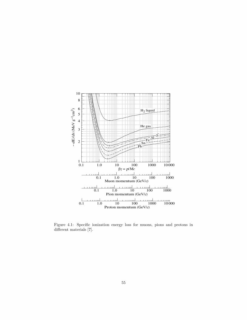
The energy loss by ionization (Figure 4.1) is thus in first approximation:

• independent of the mass of the particle;

• typically small for high energy particles (about 2 MeV/cm in water; onecan roughly assume a proportionality to the density of the material);

• proportional to 1/β2 for βγ ≤ 3 (the minimum of ionization: minimumionizing particle, or mip);

• basically constant for β > 0.96 (logarithmic increase after the minimum);

• proportional to Z/A (Z/A being about equal to 0.5 for all elements butHydrogen and the heaviest nuclei).

1The 24-year old Hans Bethe, Nobel prize in 1967 for his work on the theory of stellarnucleosynthesis, published this formula in 1930; the formula – not including the density term,added later by Fermi – was derived using quantum mechanical perturbation theory up to z2p.The description can be improved by considering corrections which correspond to higher powersof zp: Felix Block obtained in 1933 a higher-order correction proportional to z4p, not reportedin this text, and sometimes the formula is called “Bethe-Block energy loss” – although thisnaming convention has been discontinued by the Particle Data Group since 2008 [?].

54

1

2

3

4

5

6

8

10

1.0 10 100 1000 10 0000.1

Pion momentum (GeV/c)

Proton momentum (GeV/c)

1.0 10 100 10000.1

1.0 10 100 10000.1

1.0 10 100 1000 10 0000.1

!dE/d

x (M

eV g!1cm

2 )

"# = p/Mc

Muon momentum (GeV/c)

H2 liquid

He gas

CAl

FeSn

Pb

Figure 4.1: Specific ionization energy loss for muons, pions and protons indifferent materials [?].

55

In practical cases, most relativistic particles (e.g., cosmic-ray muons) havemean energy loss rates close to the minimum; they can be considered withinless than a factor of two as minimum-ionizing particles. The radiation from amip is well approximated as

1

ρ

dE

dx' 3.5

(Z

A

)MeV cm2/g .

The statistical nature of the ionizing process during the passage of a fastcharged particle through matter results in large fluctuations of the energy lossin absorbers which are thin compared with the particle range. The energyloss is distributed around the most probable value according to an asymmetricdistribution (named the Landau distribution). The average energy loss is abouttwice as large as the most probable energy loss.

The main characteristics of Eq. (4.1) can be derived classically. ?? Addhere Fernando’s exercise.

Photoluminescence. In some transparent media, part of the ionization en-ergy loss goes into the emission of visible or near-visible light by the excitationof atoms and/or molecules. This phenomenon is called photoluminescence; of-ten it results into a fast (< 100µs) excitation/deexcitation; in this case we talkof fluorescence, or scintillation2.

High-energy radiation effects

According to the classical electromagnetic theory, a charged particle emits elec-tromagnetic waves whenever it undergoes an acceleration, and the intensity ofthe emitted radiation, calculated in the so-called dipole approximation, is di-rectly proportional to the square of the acceleration.

While the dipole approximation is appropriate also in quantum electrody-namics for the description of the radiation by a particle bended by a magneticfield (synchrotron radiation), it cannot be applied in the case of interactionswith the electric fields of the atoms of the material traversed by a charged par-ticle. We speak in this case of bremsstrahlung, or braking radiation; a calculationbased on relativistic quantum mechanics has to be applied in this case – see forexample [?].

The result at first order is that the emitted energy is still (as in the classicalcase) proportional to the inverse of the square of the mass. On top of theionization energy loss described by Eq. 4.1, above βγ ∼ 1000 (which means anextremely high energy for a proton, E ∼ 1 TeV, but just E ∼ 100 GeV for amuon), radiation effects become important (Figure 4.2).

Bremsstrahlung is particularly relevant for electrons and positrons, particlesfor which the approximation starts to be inadequate at even lower energies.The average fractional energy loss by radiation for an electron of high energy

2Specialists often use definitions which distinguish between fluorescence and scintillation;this separation is, however, not universally accepted.

56

Figure 4.2: Stopping power (−dE/dx) for positive muons in copper as a func-tion of βγ = p/Mc over nine orders of magnitude in momentum (12 orders ofmagnitude in kinetic energy) [?].

(E � mec2) is approximately independent of the energy itself, and can be

described by the equation1

E

dE

dx' − 1

X0(4.2)

where X0 is called radiation length, and is characteristic of the material – forexample it is about 300 m for air at Normal Temperature and Pressure (NTP)3,about 36 cm for water, about 0.5 cm for lead; see Appendix B for a table withthe characteristics of different materials.

With good approximation

1

X0= 4

(~mec

)2

Z(Z + 1)α3na ln

(183

Z1/3

), (4.3)

where na is the density of atoms per cubic centimeter in the medium, or moresimply

1

ρX0 ' 180

A

Z2cm

(∆X0

X0< ±20% for 12 < Z < 93

). (4.4)

3NTP is commonly used as a standard condition; it is defined as air at 20◦C (293.15 K) and1 atm (101.325 kPa). Density is 1.204 kg/m3. The definition of Standard Temperature andPressure STP, another condition frequently used in physics, is defined by IUPAC (InternationalUnion of Pure and Applied Chemistry) as air at 0◦C (273.15 K) and 100 kPa.

57

Figure 4.3: Fractional energy loss per radiation length in lead as a function ofelectron or positron energy [?].

The total average energy loss by radiation increases then rapidly (linearlyin the approximation of the equation (4.2)) with increasing energy, while theaverage energy loss by collision is practically a constant. Thus, at large energiesradiation losses are much more important than collision losses (Figure 4.3).

The energy at which the radiation loss overtakes the collision loss (criticalenergy, Ec) decreases with increasing atomic number:

Ec '550 MeV

Z

(∆EcEc

< ±10% for 12 < Z < 93

). (4.5)

Critical energy for air at NTP is about 84 MeV; for water is about 74 MeV.The photons radiated by bremsstrahlung are distributed at leading order in

such a way that the differential loss per unit energy is constant, i.e.,

Nγ ∝1

Eγ

between 0 and E. This results in a divergence for Eγ → 0, which anyway doesnot contradict energy conservation.

The emitted photons are collimated: the typical he angle of emission is∼ me/E.

Cherenkov radiation

The Vavilov-Cherenkov (commonly called just Cherenkov) radiation occurs whena charged particle moves through a medium faster than the speed of light inthat medium. The total energy loss due to this process is negligible; however,Cherenkov radiation is important related to the possibility of use in detectors.

58

Figure 4.4: The emission of Cherenkov radiation by a charged particle.

The light is emitted in a coherent cone (Figure 4.4) at an angle

θc =1

nβ

from the direction of the emitting particle. The threshold velocity is thus β =1/n, where n is the refractive index of the medium. The presence of a coherentwavefront can be easily derived by using the Huygens-Fresnel principle.

The number of photons produced per unit path length and per unit energyinterval of the photons by a particle with charge zpe is

d2N

dEdx'αz2

p

~csin2 θc ' 370 sin2 θc eV−1cm−1 (4.6)

or equivalentlyd2N

dλdx'

2παz2p

λ2sin2 θc (4.7)

(the index of refraction n is in general a function of photon energy E; Cherenkovradiation is relevant when n < 1 and the medium is transparent, and thishappens close to the range of visible light).

The total energy radiated is small, some 10−4 times the energy lost by ion-ization. In the visible range (300 nm to 700 nm), the total number of emittedphotons is about 40 per meter in air, about 500 per centimeter in water. Dueto the dependence on λ, it is important that Cherenkov detectors are sensitiveclose to the ultraviolet region.

59

Figure 4.5: Multiple Coulomb scattering [?].

Dense media can be transparent not only to visible light, but also to radiowaves. The development of Cherenkov radiation in the radiowave region, dueto the interactions with matter electrons, is often referred to as the Askar’yane?ect. The e?ect has been experimentally conrmed in accelerator experimentsat SLAC in media such as sand, rock salt and ice; presently attempts are inprogress to use this effect for in particle detectors.

Transition radiation

X-ray transition radiation (XTR) occurs when a relativistic charged particlepasses from one medium to another of a different dielectric permittivity.

The energy radiated when a particle with charge zpe and γ ' 1000 crossesthe boundary between vacuum and a a different transparent medium is typicallyconcentrated in the soft x-ray range 2 keV to 40 keV.

The process is closely related to Cherenkov radiation, and also in this casethe total energy emitted is low. ?? Specify better; ask the Bari people to add afew lines with number of photons etc.

Multiple scattering

When a charged particle passes near a nucleus it undergoes a deflection which,in most cases, is accompanied by a negligible (approximately zero) loss of en-ergy. This phenomenon, called elastic scattering, is caused by the same electricinteraction between the passing particle and the Coulomb field of the nucleus.The global effect is that the path of the particle becomes a random walk (Figure4.5), and information on the original direction is partly lost – this fact can createproblems for the reconstruction of direction in tracking detectors. For very-highenergy hadrons, also hadronic cross section can contribute to the effect.

Summing up many relatively small random changes of the direction of flightfor a thin layer of traversed material, the distribution of the projected scatteringangle of a particle of unit charge can be approximated by a Gaussian distribution

60

of standard deviation (projected on a plane: one has to multiply by√

2 todetermine the variance in space):

θ0 =13.6 MeV

βcpzp

√x

X0

[1 + 0.038 ln

x

X0

].

The above expression comes from the so-called Moliere theory, and is ac-curate to some 10% or better for 10−3 < x/X0 < 100. We will obtain now asimple derivation.

?? Add here Fernando’s simple calculation of multiple scattering.The underlying assumption of a Gaussian distribution makes this approxi-

mation a crude one; in particular, large angles are underestimated by a Gaus-sian form, and some 2% of the particles can suffer more important kicks due toRutherford scattering and contribute to a sizeable tail [?].

4.1.2 Photon interactions

Photons mostly interact with matter via photoelectric effect, Compton scat-tering, and electron-positron pair production. Other processes, like Rayleighscattering and photonuclear interactions, have in general much smaller crosssections.

Photoelectric effect

The photoelectric effect is the ejection of an electron from a material after aphoton has been absorbed by that material. The ejected electron is called aphotoelectron.

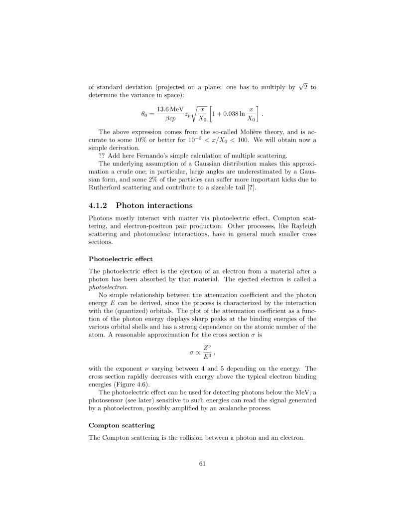
No simple relationship between the attenuation coefficient and the photonenergy E can be derived, since the process is characterized by the interactionwith the (quantized) orbitals. The plot of the attenuation coefficient as a func-tion of the photon energy displays sharp peaks at the binding energies of thevarious orbital shells and has a strong dependence on the atomic number of theatom. A reasonable approximation for the cross section σ is

σ ∝ Zν

E3,

with the exponent ν varying between 4 and 5 depending on the energy. Thecross section rapidly decreases with energy above the typical electron bindingenergies (Figure 4.6).

The photoelectric effect can be used for detecting photons below the MeV; aphotosensor (see later) sensitive to such energies can read the signal generatedby a photoelectron, possibly amplified by an avalanche process.

Compton scattering

The Compton scattering is the collision between a photon and an electron.

61

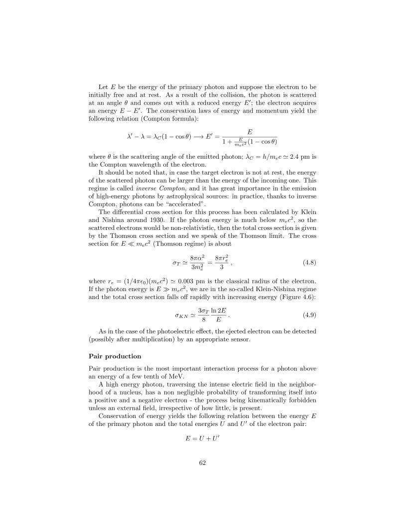
Let E be the energy of the primary photon and suppose the electron to beinitially free and at rest. As a result of the collision, the photon is scatteredat an angle θ and comes out with a reduced energy E′; the electron acquiresan energy E − E′. The conservation laws of energy and momentum yield thefollowing relation (Compton formula):

λ′ − λ = λC(1− cos θ) −→ E′ =E

1 + Emec2

(1− cos θ)

where θ is the scattering angle of the emitted photon; λC = h/mec ' 2.4 pm isthe Compton wavelength of the electron.

It should be noted that, in case the target electron is not at rest, the energyof the scattered photon can be larger than the energy of the incoming one. Thisregime is called inverse Compton, and it has great importance in the emissionof high-energy photons by astrophysical sources: in practice, thanks to inverseCompton, photons can be “accelerated”.

The differential cross section for this process has been calculated by Kleinand Nishina around 1930. If the photon energy is much below mec

2, so thescattered electrons would be non-relativistic, then the total cross section is givenby the Thomson cross section and we speak of the Thomson limit. The crosssection for E � mec

2 (Thomson regime) is about

σT '8πα2

3m2e

=8πr2

e

3, (4.8)

where re = (1/4πε0)(mec2) ' 0.003 pm is the classical radius of the electron.

If the photon energy is E � mec2, we are in the so-called Klein-Nishina regime

and the total cross section falls off rapidly with increasing energy (Figure 4.6):

σKN '3σT

8

ln 2E

E. (4.9)

As in the case of the photoelectric effect, the ejected electron can be detected(possibly after multiplication) by an appropriate sensor.

Pair production

Pair production is the most important interaction process for a photon abovean energy of a few tenth of MeV.

A high energy photon, traversing the intense electric field in the neighbor-hood of a nucleus, has a non negligible probability of transforming itself intoa positive and a negative electron - the process being kinematically forbiddenunless an external field, irrespective of how little, is present.

Conservation of energy yields the following relation between the energy Eof the primary photon and the total energies U and U ′ of the electron pair:

E = U + U ′

62

With reasonable approximation, for 1 TeV> E > 100 MeV the fraction of energyu = U/E taken by the secondary electron/positron is uniformly distributedbetween 0 and 1 (becoming peaked at the extremes as the energy increases tovalues above 1 PeV).

The cross section grows quickly from the kinematical threshold of about 1MeV to its asymptotic value reached at some 100 MeV:

σ ' 7

9

1

naX0,

where na is the density of atomic nuclei per unit volume, in such a way that theinteraction length is

λ ' 9

7X0 .

The angle of emission for the particles in the pair is is typically ∼ me/E.

Rayleigh scattering and photonuclear interactions

Rayleigh scattering (the dispersion of electromagnetic radiation by particles withradii less than or in the order of 1/10 the wavelength of the radiation) is usuallyof minor importance for the conditions of high energy particle and astroparticlephysics, but it can be important for light in the atmosphere, and thus for thedesign of instruments detecting visible light. The photonuclear effect, i.e., theexcitation of nuclei by photons, is mostly restricted to the region around 10MeV, and it may amount to as much as 10 percent of the total cross sectiondue to electrodynamic effects.

Comparison between different processes for photons

The total probability for Compton scattering decreases rapidly with increasingphoton energy, while the total probability for pair production is a slowly in-creasing function of the energy. Thus, at large energies, most of the photons areabsorbed by pair production, while at small energies most of the photons areabsorbed by Compton effect (being photoelectric effect characteristic of evensmaller energies). The absorption of photons by pair production, Compton andphotoelectric effect is compared in Figure 4.6.

As a matter of fact, above about 30 MeV the dominant process is pairproduction, and the interaction length of a photon is with extremely good ap-proximation equal to 9X0/7.

At extremely high matter densities and/or at extremely high energies (typ-ically above 1016 eV – 1018 eV, depending on the medium composition anddensity) the Landau-Pomeranchuk-Migdal effect, or simply LPM effect4, entailsa reduction of the pair production cross section, as well as of bremsstrahlung.

4Here a short qualitative description of where the LPM effect comes from ??

63

Figure 4.6: Energy dependence of the photon mass attenuation coefficient inlead tungstate (data from NIST XCOM data base).

4.1.3 Nuclear (hadronic) interactions

The nuclear force is felt by hadrons, charged and neutral; at high energies (abovea few GeV) the inelastic cross section for hadrons is dominated by nuclear in-teraction. High-energy nuclear interactions can be characterized by an inelasticinteraction length λH . Values for ρλH are typically of the order of 100 g/cm2;a listing for some common materials is provided in Appendix B.

The final state products of inelastic high-energy hadronic collisions are mostlypions, since these are the lightest hadrons. The rate of positive, negative, andneutral pions is more or less equal - as we shall see, this depende on a funda-mental symmetry of hadronic interactions, the isospin symmetry.

4.1.4 Range

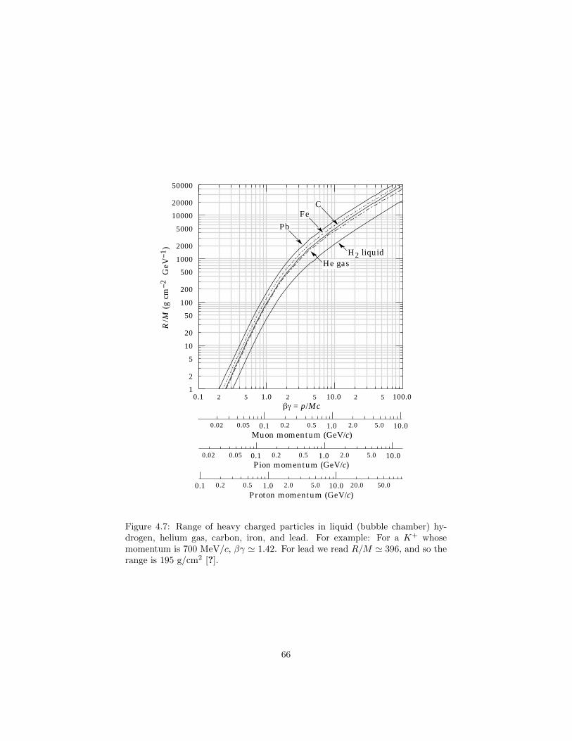
From the rate of energy loss as a function of energy, we can calculate the rateof energy loss as a function of the distance x travelled in the medium. Thisis called the Bragg curve. For charged particles, most of the ionization lossoccurs near the end of the path where the speed is smallest, and the curve hasa pronounced peak close to the end point before falling rapidly to zero at theend of the particles path length. The range R for a particle of energy E is theaverage distance traveled before reaching the energy at which the particle isabsorbed (Figure 4.7):

R =

∫ Mc2

E

1dEdx

dx .

64

Below the energy of minimum ionization (βγ < 3),

??Addhere the exercise on range by Fernando

4.2 Particle detectors

The aim of a particle detector is to measure the momenta and discover theidentity of the particles that pass through it after being produced in a collisionor a decay - an “event”. The position in space where the event occurs is knownas the interaction point.

In order to identify every particle produced by the collision, and plot thepaths they take - i.e., to “completely reconstruct the event” - it is necessaryto know the mass and momentum of the particles. The mass can be found bymeasuring the momentum and either the velocity or the energy.

The characteristics of the different instrument that allow these measurementsare presented in what follows.

4.2.1 Track detectors

A tracking detector reveals the path taken by a particle by measurements ofsampled points (hits). Momentum measurements can be made by measuringthe curvature of the track in a magnetic field, this causes the particle to curveinto a spiral orbit with a radius proportional to the momentum of the particle.This requires the calculation of the best fit of a helix to the hits (particle fit).For a particle of unit charge

p ' 0.3B⊥R ,

where B⊥ is the component of the magnetic field perpendicular to the particlevelocity, expressed in tesla (which is the order of magnitude of typical fields indetectors), the momentum p is expressed in GeV, and the radius R in meters.

A source of noise for this measurement is given by the errors in the mea-surement of the hits; another (intrinsic) noise is given by multiple scattering. Inwhat follows we will review some detectors of the trajectory of charged tracks.

Cloud chamber and bubble chamber

The cloud chamber was invented by C.T.R. Wilson the beginning of XX cen-tury, and was an instrument for reconstructing the trajectories of charged cosmicrays. The instrument is a container with a glass window, filled with air and sat-urated water vapour (Figure 4.8); the volume can be suddenly expanded, andthe adiabatic expansion causes the temperature to drop bringing the vapourto a supersaturated (metastable) state. A charged particle crossing the cham-ber produces ions, which act as seeds for the generation of droplets along thetrajectory. One can record the trajectory by taking a photographic picture. Ifthe chamber is immersed in a magnetic field B, momentum and charge can bemeasured by the curvature.

65

0.05 0.10.02 0.50.2 1.0 5.02.0 10.0Pion momentum (GeV/c)

0.1 0.50.2 1.0 5.02.0 10.0 50.020.0

Proton momentum (GeV/c)

0.050.02 0.1 0.50.2 1.0 5.02.0 10.0Muon momentum (GeV/c)

βγ = p/Mc

1

2

5

10

20

50

100

200

500

1000

2000

5000

10000

20000

50000

R/M

(g

cm−2

GeV

−1)

0.1 2 5 1.0 2 5 10.0 2 5 100.0

H2 liquidHe gas

PbFe

C

Figure 4.7: Range of heavy charged particles in liquid (bubble chamber) hy-drogen, helium gas, carbon, iron, and lead. For example: For a K+ whosemomentum is 700 MeV/c, βγ ' 1.42. For lead we read R/M ' 396, and so therange is 195 g/cm2 [?].

66

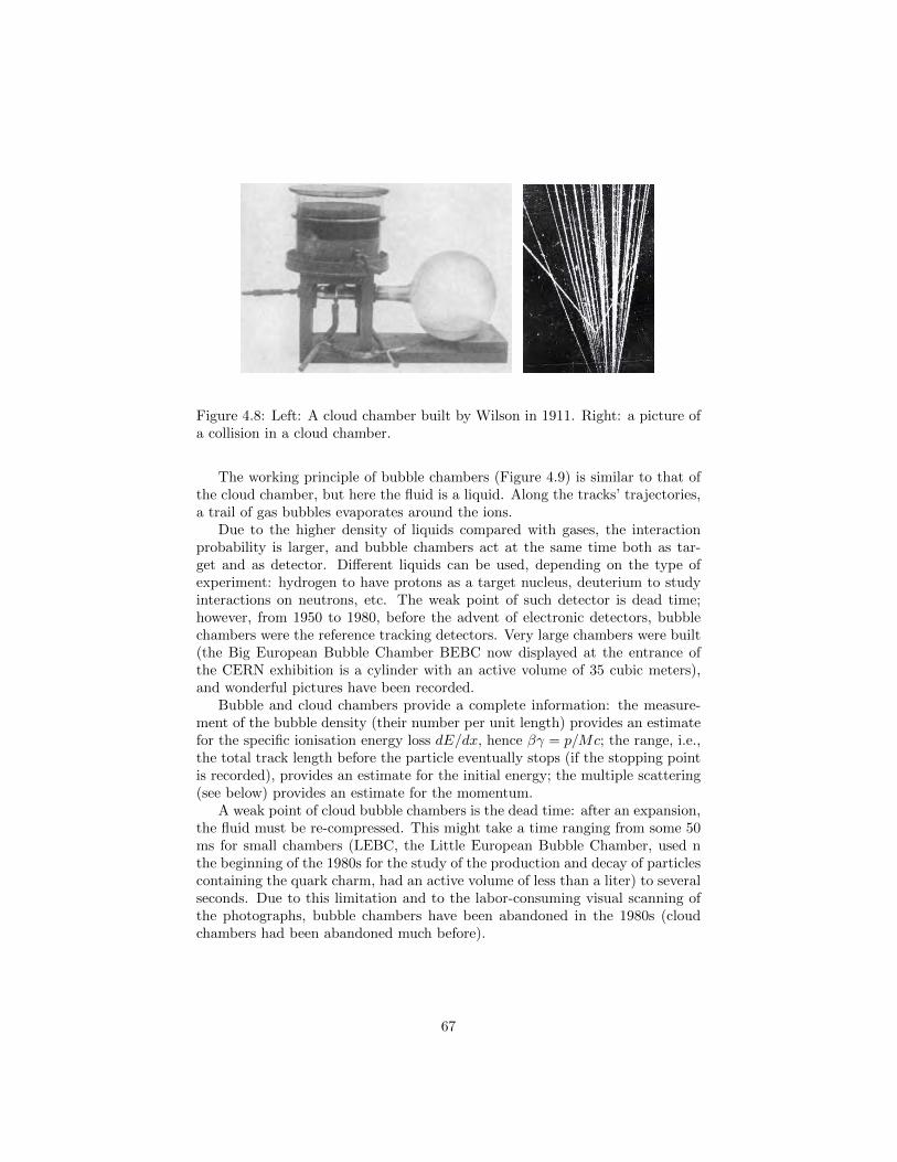
Figure 4.8: Left: A cloud chamber built by Wilson in 1911. Right: a picture ofa collision in a cloud chamber.

The working principle of bubble chambers (Figure 4.9) is similar to that ofthe cloud chamber, but here the fluid is a liquid. Along the tracks’ trajectories,a trail of gas bubbles evaporates around the ions.

Due to the higher density of liquids compared with gases, the interactionprobability is larger, and bubble chambers act at the same time both as tar-get and as detector. Different liquids can be used, depending on the type ofexperiment: hydrogen to have protons as a target nucleus, deuterium to studyinteractions on neutrons, etc. The weak point of such detector is dead time;however, from 1950 to 1980, before the advent of electronic detectors, bubblechambers were the reference tracking detectors. Very large chambers were built(the Big European Bubble Chamber BEBC now displayed at the entrance ofthe CERN exhibition is a cylinder with an active volume of 35 cubic meters),and wonderful pictures have been recorded.

Bubble and cloud chambers provide a complete information: the measure-ment of the bubble density (their number per unit length) provides an estimatefor the specific ionisation energy loss dE/dx, hence βγ = p/Mc; the range, i.e.,the total track length before the particle eventually stops (if the stopping pointis recorded), provides an estimate for the initial energy; the multiple scattering(see below) provides an estimate for the momentum.

A weak point of cloud bubble chambers is the dead time: after an expansion,the fluid must be re-compressed. This might take a time ranging from some 50ms for small chambers (LEBC, the Little European Bubble Chamber, used nthe beginning of the 1980s for the study of the production and decay of particlescontaining the quark charm, had an active volume of less than a liter) to severalseconds. Due to this limitation and to the labor-consuming visual scanning ofthe photographs, bubble chambers have been abandoned in the 1980s (cloudchambers had been abandoned much before).

67

Figure 4.9: Left: the BEBC bubble chamber. Center: A picture taken in BEBC,and Right: its interpretation.

Nuclear emulsions

A nuclear emulsion plate is a photographic plate with a particularly thick emul-sion layer and with a very uniform grain size. Like bubble chambers and cloudchambers they record the tracks of charged particles passing through, by chang-ing the chemical status of grains that have absorbed photons (which makes themvisible after photographic processing). They are compact, have high density andproduce a cumulative record, but have the disadvantage that the plates mustbe developed before the tracks can be observed.

Nuclear emulsion have very good space resolution of the order of few µm.They had great importance in the beginning of cosmic-ray physics; they are stillunsurpassed from what is related to single-point space resolution, and are stillused for example in the OPERA experiment at Gran Sasso5.

Ionization counter, proportional counter and Geiger-Muller counter

These three kinds of detectors have the same principle of operation: they consistof a tube filled with a gas, with a charged metal wire inside (Figure 4.10). Whena charged particle enters the detector, it ionizes the gas, and the ions and theelectrons can be collected by the wire and by the walls (the mobility of electronsbeing larger than the mobility of ions, it is convenient that the wire’s potentialis positive). The electrical signal of the wire can be amplified and read by meansof an amperometer. The tension V of the wire must be larger than a thresholdbelow which ions and electrons spontaneously recombine.

Depending on the tension V of the wire, one can have three different regimes:

• The ionization chamber regime when V < I/e (where I is the ionizationenergy of the gas, and e the electron charge). The primary ions produced

5OPERA ??

68

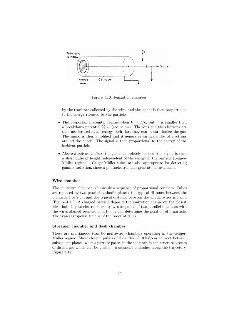
Figure 4.10: Ionization chamber.

by the track are collected by the wire, and the signal is then proportionalto the energy released by the particle.

• The proportional counter regime when V > I/e, but V is smaller thana breakdown potential VGM (see below). The ions and the electrons arethen accelerated at an energy such that they can in turn ionize the gas.The signal is thus amplified and it generates an avalanche of electronsaround the anode. The signal is then proportional to the energy of theincident particle.

• Above a potential VGM , the gas is completely ionized; the signal is thena short pulse of height independent of the energy of the particle (Geiger-Muller regime). Geiger-Muller tubes are also appropriate for detectinggamma radiation, since a photoelectron can generate an avalanche.

Wire chamber

The multiwire chamber is basically a sequence of proportional counters. Tubesare replaced by two parallel cathodic planes; the typical distance between theplanes is 1 to 2 cm and the typical distance between the anodic wires is 1 mm(Figure 4.11). A charged particle deposits the ionization charge on the closestwire, inducing an electric current; by a sequence of two parallel detectors withthe wires aligned perpendicularly one can determine the position of a particle.The typical response time is of the order of 30 ns.

Streamer chamber and flash chamber

These are multianode (can be multiwire) chambers operating in the Geiger-Muller regime. Short electric pulses of the order of 10 kV/cm are sent betweensubsequent planes; when a particle passes in the chamber, it can generate a seriesof discharges which can be visible – a sequence of flashes along the trajectory,Figure 4.12.

69

Figure 4.11: Scheme of a multiwire chamber (source: wikimedia commons).

Figure 4.12: The flash chamber built by the Laboratorio de Instrumentacao ePariticulas (LIP) fro didactical purposes.

Drift chamber

The drift chamber is a multiwire chamber in which spatial resolution is achievedby measuring the time electrons need to reach the anode wire, starting from themoment that the ionizing particle traversed the detector. This results in widerwire spacing with respect to what can be obtained using multiwire proportionalchambers. Fewer channels have to be equipped with electronics, but the overallspace resolution can be comparable; in addition, they are often coupled to high-precision space measurement devices like silicon detectors (see below).

Drift chambers use longer drift distances, hence can be slower than multiwirechambers [?]. Since the drift distance can be long and drift velocity needs tobe well known, the shape and constancy of the electric field needs to be carefuladjusted and controlled. To do this, besides the anode (signal) wires, thickfield-shaping cathode wires called field wires are often used.

An extreme case is given by time projection chambers (TPC), for which driftlengths can be very large (up to 2 m), and the sense wires are arranged in oneend face; the signals induced in pads or strips near the sense wire plane can beused to obtain three-dimensional information.

Semiconductor detectors

Silicon microstrip detectors are are solid-state particle detectors, whose principleof operation is similar to that of a ionization chamber: the passage of ionizing

70

Figure 4.13: Scheme of a silicon microstrip detector.

particles produces in them a number of electron-hole pairs proportional to theenergy released.

The electron-hole pairs are collected thanks to an electric field, and generatean electrical signal.

The main feature of silicon detectors is the small energy required to createa electron-hole pair – about 3.6 eV, compared with about 30 eV necessary toionize an atom in an Ar gas ionization chamber.

Furthermore, compared to gaseous detectors, they are characterized by ahigh density and a high stopping power, much greater than that of the gasdetectors: they can thus be very thin, typically about 300 µm.

The general pattern of a silicon microstrip detector is shown in Figure 4.13.The distance between two adjacent strips is the pitch and can be of the order

of 100 µm, as the width of each strip.From the signal collected on the strip one can tell if a particle has passed

through the detector. The accuracy can be smaller than the size and the pitch:the charge sharing between adjacent strips improves the resolution to some10µm. As in the case of mutiwire chambers, the usual geometry involves adja-cent parallel planes of mutually perpendicular strips.

A recent implementation of semiconductor detectors is the Silicon pixel de-tector. Wafers of silicon are segmented into little squares (the pixels) that are assmall as 100 µm on a side. Electronics is more expensive (however with moderntechnology it can be bonded to the sensors themselves); the advantage is thatone can measure directly the hits getting rid of ambiguities.

Scintillators

Scintillators are among the oldest particle detectors. They are slabs of transpar-ent material, organic or inorganic; the ionization induces fluorescence, and thelight is conveyed towards a photosensors (photosensors will be described later).The light yield is large (can be as large as 104 photons per MeV of energy de-

71

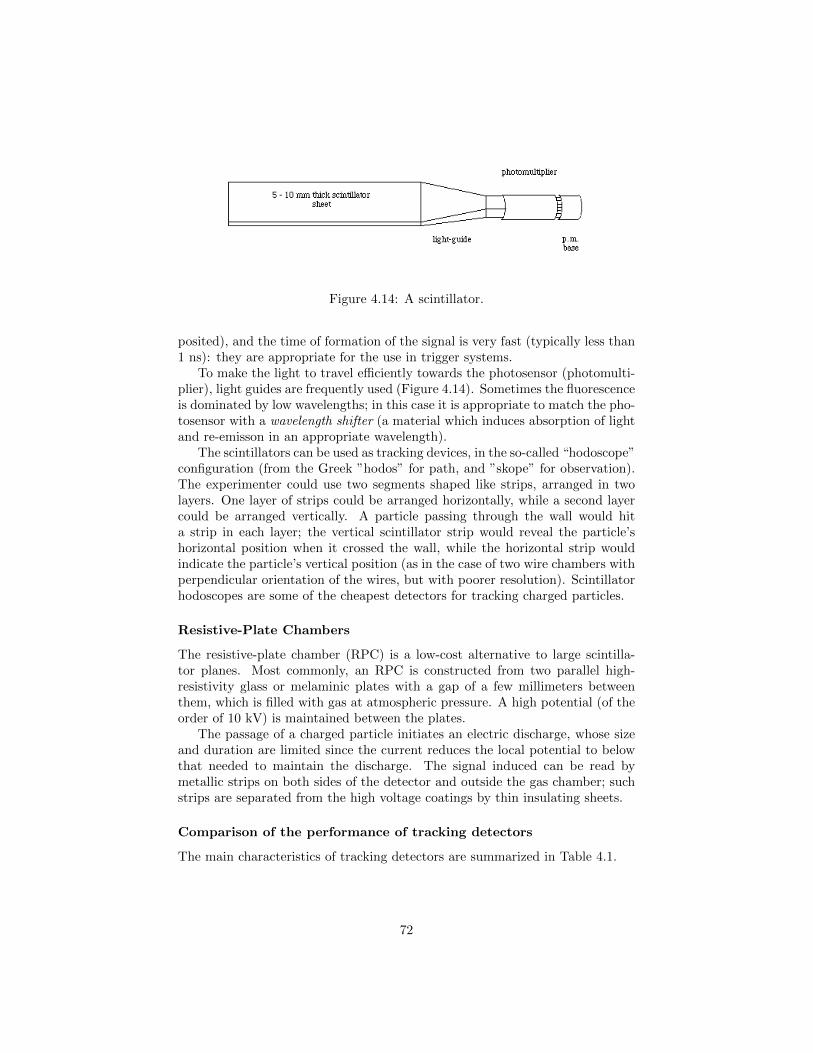
Figure 4.14: A scintillator.

posited), and the time of formation of the signal is very fast (typically less than1 ns): they are appropriate for the use in trigger systems.

To make the light to travel efficiently towards the photosensor (photomulti-plier), light guides are frequently used (Figure 4.14). Sometimes the fluorescenceis dominated by low wavelengths; in this case it is appropriate to match the pho-tosensor with a wavelength shifter (a material which induces absorption of lightand re-emisson in an appropriate wavelength).

The scintillators can be used as tracking devices, in the so-called “hodoscope”configuration (from the Greek ”hodos” for path, and ”skope” for observation).The experimenter could use two segments shaped like strips, arranged in twolayers. One layer of strips could be arranged horizontally, while a second layercould be arranged vertically. A particle passing through the wall would hita strip in each layer; the vertical scintillator strip would reveal the particle’shorizontal position when it crossed the wall, while the horizontal strip wouldindicate the particle’s vertical position (as in the case of two wire chambers withperpendicular orientation of the wires, but with poorer resolution). Scintillatorhodoscopes are some of the cheapest detectors for tracking charged particles.

Resistive-Plate Chambers

The resistive-plate chamber (RPC) is a low-cost alternative to large scintilla-tor planes. Most commonly, an RPC is constructed from two parallel high-resistivity glass or melaminic plates with a gap of a few millimeters betweenthem, which is filled with gas at atmospheric pressure. A high potential (of theorder of 10 kV) is maintained between the plates.

The passage of a charged particle initiates an electric discharge, whose sizeand duration are limited since the current reduces the local potential to belowthat needed to maintain the discharge. The signal induced can be read bymetallic strips on both sides of the detector and outside the gas chamber; suchstrips are separated from the high voltage coatings by thin insulating sheets.

Comparison of the performance of tracking detectors

The main characteristics of tracking detectors are summarized in Table 4.1.

72

Detector type Space resolution Time resolution Dead time

RPC ≤ 10 mm ∼ 1ns –Scintillation counter 10 mm 0.1 ns 10 nsEmulsion 1µm – –Bubble chamber 10− 100µm 1 ms 50 ms- 1sProportional chamber 50− 100µm 2 ns 20-200 nsDrift chamber 50− 100µm few ns 20-200 nsSilicon strip Pitch/5 (few µm) few ns 50 nsSilicon pixel 10 µm few ns 50 ns

Table 4.1: Typical characteristics of different kinds of tracking detectors (datacome from [?]).

4.2.2 Photosensors

Most detectors in particle physics and astrophysics rely on the detection ofphotons near the visible range, i.e., in the eV energy range. This range coversscintillation and Cherenkov radiation as well as the light detected in manyastronomical observations.

Essentially, one needs to extract a measurable signal from a (usually verysmall) number of incident photons. This goal can be achieved by generating aprimary photoelectron or electron-hole pair by an incident photon (typically byphotoelectric effect), amplifying the signal to a detectable level (usually by asequence of avalanche processes), and collecting the secondary charges to formthe electrical signal.

The important characteristics of a photodetector include the quantum effi-ciency QE (the probability that a primary photon generates a photoelectron),the collection efficiency C (the overall acceptance factor), the gain G (the num-ber of electrons collected for each photoelectron generated), Dark Noise (theelectrical signal when there is no photon), and the intrinsic response time of thedetector.

Several kinds of photosensor are used in experiments.

Photomultiplier tubes

Photomultiplier tubes (photomultipliers or PMTs for short) are detectors oflight in the ultraviolet, visible, and near-infrared ranges of the electromagneticspectrum; they are the oldest photon detectors used in high energy particle andastroparticle physics.

They are constructed (Figure 4.15) from a glass envelope with a high vacuuminside, housing a photocathode, several intermediate electrodes called dynodes,and an anode. Incident photons strike the photocathode material, which ispresent as a thin deposit on the entry window of the device, with electrons

73

Figure 4.15: Scheme of a photomultiplier.

being produced as a consequence of the photoelectric effect. These electronsare directed by the focusing electrode toward the electron multiplier, whereelectrons are multiplied by the process of secondary emission.

The electron multiplier consists of a number of dynodes. Each dynode isheld at a more positive voltage than the previous one (the typical total voltagein the avalanche process being of 1kV - 2kV). The electrons leave the photocath-ode, having the energy of the incoming photon (minus the work function of thephotocathode). As the electrons move toward the first dynode, they are accel-erated by the electric field and arrive with much greater energy. Upon strikingthe first dynode, more low energy electrons are emitted, and these electrons inturn are accelerated towards the second dynode. The geometry of the dynodechain is such that a cascade occurs with an ever-increasing number of electronsbeing produced at each stage. Finally, the electrons reach the anode, where theaccumulation of charge results in a sharp current pulse indicating the arrival ofa photon at the photocathode.

The photocathodes can be made of a variety of materials, with differentproperties. Typically these materials have low work function.

The typical quantum efficiency of a photomultiplier is about 30% in therange from 300 nm to 800 nm of wavelength for the light, and the gain G is inthe range 105 to 106.

A recent improvement to the photomultiplier was obtained thanks to hybridphoton detectors (HPD), in which a vacuum PMT is coupled to a Silicon sensor.A photoelectron ejected from the photocathode is accelerated through a poten-tial difference of about V ' 20 kV before it impinges on a silicon sensor/anode.The number of electron-hole pairs that can be created in a single accelerationstep is G ∼ eV/(3.6 eV), the denominator being the mean energy required tocreate an electron-hole pair.

Gaseous photon detectors

In gaseous photomultipliers (GPM) a photoelectron in a suitable gas mixture(a gas with low photoionization work function, like the tetra dimethyl-amine

74

ethylene TMAE) starts an avalanche in a high-field region, producing a largenumber of secondary ionization electrons. The charge multiplication and collec-tion processes are identical to those employed in gaseous tracking detectors.

Since GPMs can have a good space resolution and can be made into flatpanels to cover large areas, they are often used as position-sensitive photondetectors. Many of the ring imaging Cherenkov (RICH) detectors (see later)use GPM as sensors.

Solid-state photon detectors

Semiconductor photodiodes were developed during World War II, approximatelyat the same time when the photomultiplier tube became a commercial prod-uct. Only in recent years, however, a technique was engineered which allowsthe Geiger-mode avalanche in Silicon, and the semiconductor photodetectorsreached sensitivities comparable to photomultiplier tubes. Solid-state photode-tectors (often called SiPM) are more compact, lightweight, and they might be-come cheaper than traditional PMTs in the near future. They also allow finepixelization, of the order of 1 mm× 1 mm, are easy to integrate into largesystems, and can operate at low electric potentials.

One of the most promising recent developments in the field is the construc-tion of large arrays of tiny avalanche photodiodes (APD) packed over a smallarea and operated in Geiger mode.

?? Specify advantages and disadvantages of SiPM and solid-state photondetectors.

4.2.3 Cherenkov detectors

Cherenkov detectors use photodetectors to detect Cherenkov photons. Theyield of Cherenkov radiation us usually generous so to make these detectorsperformant.

If one does not need particle identification, a cheap medium (radiator) withlarge n can be used so to have a threshold for the emission as low as possible.A typical radiator is water, with n ' 1.33. The IceCube detector in Antarcticauses ice as a radiator (the photomultipliers are embedded in the ice).

Since the photon yield and the emission angle depend on the mass of theparticle, some Cherenkov detectors are also used for particle identification.

Threshold Cherenkov detectors make a yes/no decision based on whethera particle is above or below the Cherenkov threshold velocity c/n – this factdepends on the velocity; if the momentum has been measured, it is in practicea threshold measurement on the value of the mass. A more advanced versionof such detectors uses the number of observed photoelectrons to discriminatebetween species.

Imaging Cherenkov detectors measure the ring-correlated angles of emis-sion of the individual Cherenkov photons. Since low-energy photon detectorscan measure the position (and, sometimes, the arrival time) of the individualCherenkov photons, the photons must be “imaged” onto a detector so that their

75

angles can be derived. Typically the optics map the Cherenkov cone onto (aportion of) a conical section at the photodetector.

Among imaging detectors, in RICH detectors, a cone of Cherenkov light isproduced when a high speed charged particle traverses a suitable gaseous orliquid radiator. This light cone is detected on a position sensitive planar photondetector, which allows reconstructing a ring or disc, the radius of which is a mea-sure for the Cherenkov emission angle. Both focusing and proximity-focusingdetectors are in use. In a focusing detector, the photons are collected by aspherical mirror and focused onto the photon detector placed at the focal plane.The result is a conic section (a circle for normal incidence); it can be demon-strated that the radius of the circle is independent of the emission point alongthe particle track. This scheme is suitable for low refractive index radiators, asgases, due to the larger radiator length needed to create enough photons. In themore compact proximity-focusing design, a thin radiator volume emits a coneof Cherenkov light which traverses a small distance - the proximity gap - and isdetected on the photon detector plane. The image is a ring of light, the radiusof which is defined by the Cherenkov emission angle and the proximity gap.

Atmospheric Cherenkov telescopes for high-energy γ astrophysics are alsoin use. If one uses a parabolic telescope, again the projection of the emissionby a particle along its trajectory is a conical section in the focal plane. Ifthe particle has generated a shower, the projection is a spot, whose shape canallow distinguishing if the primary particle was a hadron or an electromagneticparticle (electron, positron or photon).

4.2.4 Transition radiation detectors

The main problem in the transition radiation detectors (TRD) is given by thelow number of photons. In order to intensify the photon flux, periodic arrange-ments of a large number of foils are in use, interleaved by X- ray detectors, e.g.multiwire proportional chambers filled with xenon or a xenon/CO2 mixture.Thin foils of lithium, polyethylene or carbon are common. Randomly spacedradiators are also in use, like foams.

4.2.5 Calorimeters

Once entering an absorbing medium, particles undergo successive interactionsand decays, until their energy is degraded. Calorimeters are blocks of matterin which the energy a particle is measured through the absorption to the levelof detectable atomic ionizations and excitations. Such detectors can be used tomeasure not only the energy, but also the spatial position, the direction and, insome cases, the nature of the primary particle.

Electromagnetic showers

Electrons of large energy lose most of their energy by radiation. Hence by theinteraction of high energy electrons with matter only a small fraction of the

76

energy is dissipated, while a large portion is spent in the production of photonsof high energy. The secondary photons, in turn, undergo pair production (or,at lower energies, Compton scattering); in the first case, electrons and positronscan in turn radiate. This phenomenon continues generating cascades (showers)of electromagnetic particles; at each step the number of particles increases whilethe average energy decreases, until the energy falls below the critical energy.

Given the characteristics of the interactions of electrons/positrons and ofphotons with matter, it is natural to describe the process of electromagneticcascades in terms of the scaled distance

t =x

X0

and of the scaled energy

ε =E

Ec;

since the opening angles for Bremsstrahlung and pair production are small, theprocess can be in first approximation (above the critical energy) considered asone-dimensional (the lateral spread will be discussed at the end of this section).

A simple approximation, by Heitler, assumes that:

• the incoming charged particles have a starting energy E0 much larger thanthe critical energy Ec;

• each electron travels one radiation length and then gives up half of itsenergy to a bremsstrahlung photon;

• each photon travels one radiation length creates an electron-positron pairwith each particle carrying away half the energy of the original photon.

In the above model, asymptotic formulas for radiation and pair productionare assumed to be valid; the Compton effect and the collision processes areneglected. The branching stops abruptly when E = Ec, and then electrons andpositrons lose their energy by ionization.

The model is schematically shown in Figure 4.16. This simple branchingmodel suggests that after t radiation lengths the shower will contain 2t particles.There will be roughly equal numbers electrons, positrons and photons each withan average energy given by

E(t) = E0/2t .

The cascading process will stop abruptly when E(t) = Ec. The thickness ofabsorber at which the cascade ceases, tmax, can be written in terms of theinitial and critical energies:

tmax =ln(E0/Ec)

ln 2,

and the number of particles at this point will be

Nmax =E0

Ec= y .

77

Figure 4.16: Scheme of the Heitler approximation for the development of anelectromagnetic shower.

Incident electron Incident photonPeak of shower tmax 1.0× (ln y − 1) 1.0× (ln y − 0.5)Centre of gravity tmed tmax + 1.4 tmax + 1.7Number of e+ and e− at peak 0.3y/

√ln y − 0.37 0.3y/

√ln y − 0.31

Total track length y y

Table 4.2: Shower parameters according to Rossi approximation B.

The model suggests that the shower depth at the maximum varies as thelogarithm of the primary energy, a feature that emerges from more sophisticatedmodels of the process and is observed experimentally.

Rossi [?] computed analytically the development of a shower in the so-called ”approximation B” in which electrons lose energy by ionization andbremsstrahlung (described by asymptotical formulae); photons undergo pairproduction, also described by asymptotical formulae. All the process is 1-dimensional. The results of the “Rossi approximation B” are summarized inthe Table 4.2. In Rossi’s approximation, the number of particles grows expo-nentially in the beginning and up to the maximum, and then decreases as shownin Figure 4.17 and Figure 4.18.

A common parametrization of the longitudinal profile for a shower of initialenergy E0 is

dE

dt= E0

β

Γ(α)(βt)α−1e−βt ,

78

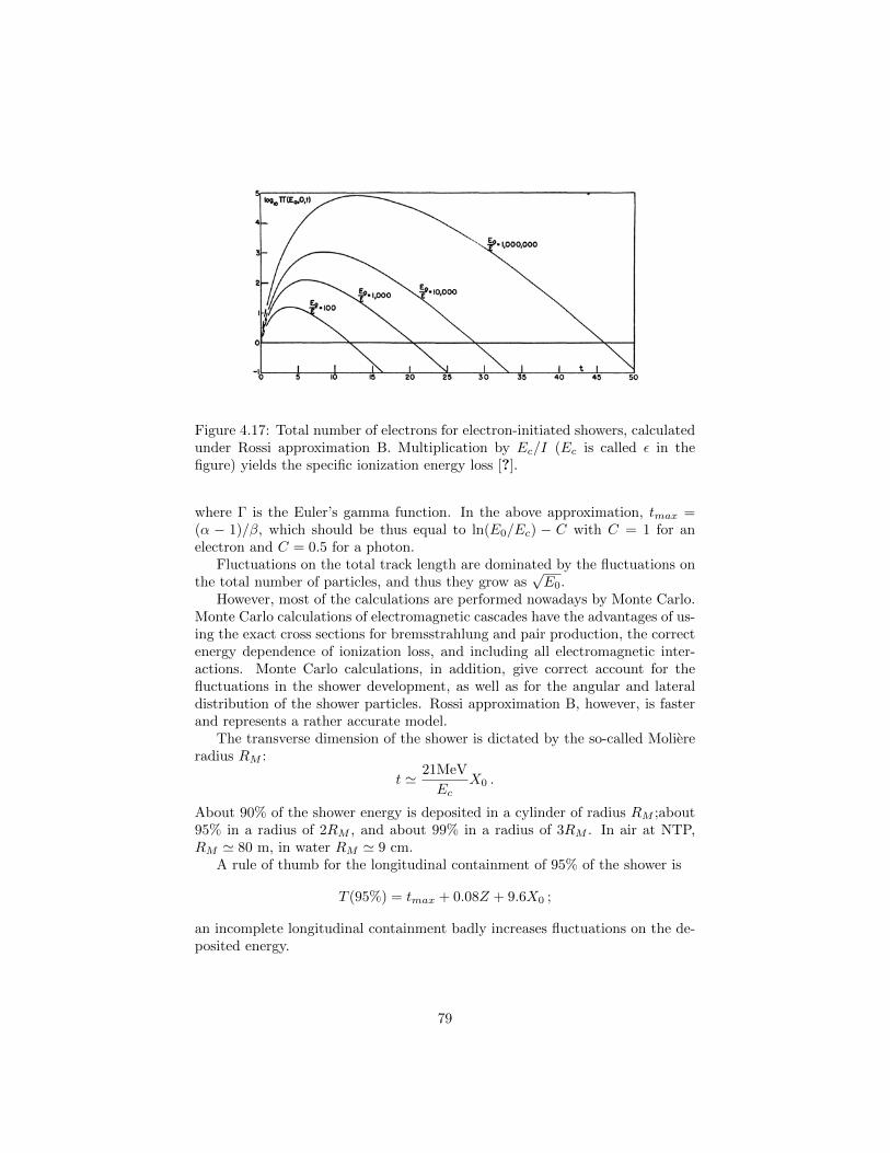
Figure 4.17: Total number of electrons for electron-initiated showers, calculatedunder Rossi approximation B. Multiplication by Ec/I (Ec is called ε in thefigure) yields the specific ionization energy loss [?].

where Γ is the Euler’s gamma function. In the above approximation, tmax =(α − 1)/β, which should be thus equal to ln(E0/Ec) − C with C = 1 for anelectron and C = 0.5 for a photon.

Fluctuations on the total track length are dominated by the fluctuations onthe total number of particles, and thus they grow as

√E0.

However, most of the calculations are performed nowadays by Monte Carlo.Monte Carlo calculations of electromagnetic cascades have the advantages of us-ing the exact cross sections for bremsstrahlung and pair production, the correctenergy dependence of ionization loss, and including all electromagnetic inter-actions. Monte Carlo calculations, in addition, give correct account for thefluctuations in the shower development, as well as for the angular and lateraldistribution of the shower particles. Rossi approximation B, however, is fasterand represents a rather accurate model.

The transverse dimension of the shower is dictated by the so-called Moliereradius RM :

t ' 21MeV

EcX0 .

About 90% of the shower energy is deposited in a cylinder of radius RM ;about95% in a radius of 2RM , and about 99% in a radius of 3RM . In air at NTP,RM ' 80 m, in water RM ' 9 cm.

A rule of thumb for the longitudinal containment of 95% of the shower is

T (95%) = tmax + 0.08Z + 9.6X0 ;

an incomplete longitudinal containment badly increases fluctuations on the de-posited energy.

79

0.000

0.025

0.050

0.075

0.100

0.125

0

20

40

60

80

100

(1/

E0)

dE

/d

t

t = depth in radiation lengths

Nu

mbe

r cr

ossi

ng

plan

e

30 GeV electronincident on iron

Energy

Photons× 1/6.8

Electrons

0 5 10 15 20

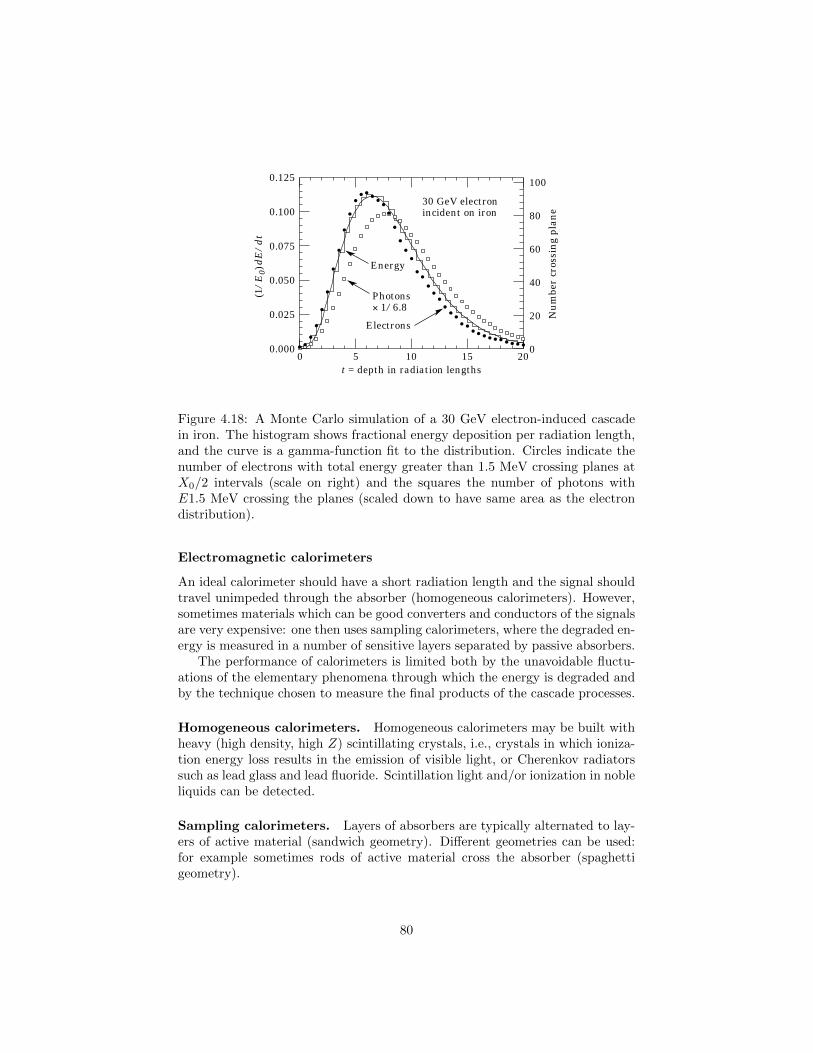
Figure 4.18: A Monte Carlo simulation of a 30 GeV electron-induced cascadein iron. The histogram shows fractional energy deposition per radiation length,and the curve is a gamma-function fit to the distribution. Circles indicate thenumber of electrons with total energy greater than 1.5 MeV crossing planes atX0/2 intervals (scale on right) and the squares the number of photons withE1.5 MeV crossing the planes (scaled down to have same area as the electrondistribution).

Electromagnetic calorimeters

An ideal calorimeter should have a short radiation length and the signal shouldtravel unimpeded through the absorber (homogeneous calorimeters). However,sometimes materials which can be good converters and conductors of the signalsare very expensive: one then uses sampling calorimeters, where the degraded en-ergy is measured in a number of sensitive layers separated by passive absorbers.

The performance of calorimeters is limited both by the unavoidable fluctu-ations of the elementary phenomena through which the energy is degraded andby the technique chosen to measure the final products of the cascade processes.

Homogeneous calorimeters. Homogeneous calorimeters may be built withheavy (high density, high Z) scintillating crystals, i.e., crystals in which ioniza-tion energy loss results in the emission of visible light, or Cherenkov radiatorssuch as lead glass and lead fluoride. Scintillation light and/or ionization in nobleliquids can be detected.

Sampling calorimeters. Layers of absorbers are typically alternated to lay-ers of active material (sandwich geometry). Different geometries can be used:for example sometimes rods of active material cross the absorber (spaghettigeometry).

80

Converters have high density, short radiation length. Typical materials areIron (Fe), Lead, Uranium. Typical active materials are plastic scintillator, Sili-con, liquid ionization chamber gas detectors.

Disadvantages of sampling calorimeters are that only part of the depositedparticle energy is detected in the active layers, typically a few percent (one ortwo orders of magnitude less for gas detectors). These sampling fluctuationstypically result in a worse energy resolution for sampling calorimeters.

Electromagnetic calorimeters: comparison of the performance. Thefractional energy resolution ∆E/E of a calorimeter can be parametrized as

∆E/E =a√E⊕ b⊕ c

E,

where ⊕ represents addition in quadrature. The stochastic term a representsstatistics-related intrinsic fluctuations in the shower, photoelectron statistics,dead material at the front of the calorimeter, and sampling fluctuations – weremind that the number of particles is roughly proportional to the energy, andthus the Poisson statistics gives fluctuations ∝

√E. While a is at a few percent

level for a homogeneous calorimeter, it is typically 10% for sampling calorime-ters. The main contributions to the systematic, or constant, term b, are detectornon-uniformity and calibration uncertainty. In the case of the hadronic cascadesdiscussed below, non-compensation (?? define) also contributes to the constantterm. The constant term b can be reduced to below one percent. The term c isdue to electronic noise. Some of the above terms can be negligible in calorime-ters.

The best energy resolution for electromagnetic shower measurement is ob-tained in total absorption homogeneous calorimeters, e.g., calorimeters builtwith heavy crystal scintillators like the Bi4Ge3O12, called BGO). These areused when ultimate performance is pursued. A relatively cheap scintillator withrelatively short X0 is the Cesium Iodide CsI, which becomes more luminescentwhen activated with Tallium, and is called CsI(Tl); this is frequently used fordosimetry in medical applications.

Energy resolutions for some homogeneous and sampling calorimeters arelisted in Table 4.3.

Hadronic showers and calorimeters

The concept of hadronic showers is similar to the concept of electromagneticshowers: primary hadrons can undergo a sequence of interactions and decayscreating a cascade. However, on top of electromagnetic interactions one has nownuclear reactions. In addition, in hadronic collisions with nuclei of the material,a significant part of the primary energy is consumed in the nuclear processes(excitation, emission nucleons low energy etc.). One thus needs ad-hoc MonteCarlo corrections to account for the energy lost, and fluctuations are larger.The development of appropriate Monte Carlo codes for hadronic interactions hasbeen a problem in itself, and still the the calculation require huge computational

81

Technology (experiment) Depth (X0) Energy resolution

BGO (L3) 22 2%√E ⊕ 0.7%

CsI (kTeV) 27 2%√E ⊕ 0.45%

PBWO4 (CMS) 25 3%√E ⊕ 0.5%⊕ 0.2%/E

Lead glass (DELPHI, OPAL) 20 5%√E

Scintillator/Pb (CDF) 18 18.5%√E

Liquid Ar/Pb (SLD) 21 12%√E

Table 4.3: Main characteristics of some electromagnetic calorimeters (data from[?]).

loads. At the end of a hadronic cascade, most of the particles are pions, andone third of the pions are neutral and decay almost istantaneously (τ ∼ 10−16

s) into a pair of photons; thus in average one third of the hadronic cascade (butit can be more or less, subject to fluctuations) is indeed electromagnetic.

In first approximation, the development of the shower can be described bythe inelastic hadronic interaction length λH ; however, the approximation isworse than the scaling of electromagnetic reactions with X0.

Detectors capable to absorb hadrons and detect a signal related to it weredeveloped around 1950 for the study of cosmic rays. It was assumed that theenergy of the incident particle was proportional to the multiplicity of chargedparticles.

Most large hadron calorimeters are sampling calorimeters which are parts ofcomplicated detectors at colliding beam facilities. Typically, the basic structureof plates is absorber (Fe, Pb, Cu, or Occasionally U or W) alternating withplastic scintillators (plates, tiles, bars), liquid argon (LAr), or gaseous detectors(Figure 4.19). The ionization is measured directly, as in LAr calorimeters, orvia scintillation light observed by photodetectors (usually photomultipliers).

The fluctuations in the invisible energy and in the and hadronic componentof a shower contribute to the resolution of hadron calorimeters. As for the sameenergy of the incident particle the energy measurable in a hadronic showeris less than that in the electromagnetic part, the response to hadrons is notcompensated with respect to the response to electromagnetic particles (or tothe electromagnetic part of the hadronic shower).

Due to all these problems, typical fractional energy resolutions are in theorder of 30%/

√E to 50%/

√E.

4.3 High-energy particles

If we want to use a beam of particles as a microscope, like Rutherford did inhis experiment, the minimum distance we can sample (for example, to probe a

82

(a) (b)

W (Cu) absorber

LAr filledtubes

Hadrons zr

scintillatortile

waveshifter fiber

PMT

Hadrons

Figure 4.19: The hadronic calorimeters of the ATLAS experiments at LHC.

possible substructure in matter) decreases with increasing energy. According tode Broglie’s equation, the relation between the momentum p and the wavelengthλ of a wave packet is given by

λ =h

p.

Therefore, larger momenta correspond to shorter wavelengths and access tosmaller structures. Particle acceleration is thus a fundamental tool for researchin physics.

In addition, it is possible to use high-energy particles to produce new parti-cles in collisions. This requires the more energy the more massive the particleswe want to produce are.

4.3.1 Artificial accelerators

A particle accelerator is an instrument using electromagnetic fields acceleratecharged particles at high energies.

There are two schemes of collision:

• collision of a beam with another beam running in opposite direction (col-lider experiments);

• collision with a fixed target (fixed-target experiments).

We also distinguish two main categories of accelerators depending on the ge-ometry: linear accelerators and circular accelerators. In linear accelerators thebremsstrahlung energy loss is much reduced since there is no centripetal accel-eration, but particles are wasted after a collision, while in circular acceleratorsthe particles which did not interact can be re-used.

83

The center of mass energy ECM sets the scale for the maximum mass ofthe particles we can produce (the actual value being in general smaller due toconstraints related to conservation laws). We want now to compare fixed targetand colliding beam experiments concerning the available energy.

In the case of beam-target collisions between two particles of mass m andenergy E,

ECM '√

2mE .

This means that, in the case of a fixed target experiment, the center of massenergy grows only with square root of E. In beam-beam collisions, instead,

ECM = 2E .

Therefore, it is much more efficient to use two beams in opposite directions. Asa result, most of the recent experiments at accelerators are done at colliders.

Making two beams to collide, however, is not trivial: one must control thefact that the beams tend to defocus due to mutual repulsion. In addition, theLiouville theorem states that the phase space volume (the product of the spreadin terms of the space coordinates times the spread in the momentum coordinate)of an isolated beam is constant: reducing the momentum dispersion is done atthe expense of the space dispersion – and one needs small space dispersion inorder that the particles in the beam actually collide. Beating the Liouvilletheorem requires feedback on the beam itself.

Since beams are circulated for several hours, circular accelerators are basedon beams of stable particles and antiparticles, such as electrons, protons, andtheir antiparticles. In the future, muon colliders ??

The accelerators and detectors are often situated underground in order toprovide the maximal shielding possible from natural radiation such as cosmicrays that would otherwise mask the events taking place inside the detector.

Acceleration methods

A particle of charge q and speed ~v in an electric field ~E and a magnetic field ~Bfeels a force

~F = q( ~E + ~v × ~B) .

The electric field can thus accelerate the particle; the work by the magneticfield is zero, nevertheless the magnetic field can be used to control the particle’strajectory. For example, a magnetic field perpendicular to ~v can constrain theparticle along a circular trajectory perpendicular to ~B.

An acceleration line (which corresponds roughly to a linear accelerator)works as follows. In a beam pipe (a cylindrical tube in which vacuum hasbeen made) cylindrical electrodes are aligned. A pulsed (radiofrequency RF)source of electromotive force V is applied. Thus particles are accelerated whenpassing to the RF cavity (Figure 4.20); the period is adjusted in such a waythat half of the period corresponds of the time needed to the particle to crossthe cavity.

84

Figure 4.20: Scheme of an acceleration line displayed at two different times(source: wikimedia commons).

To have a large number of collisions, it is useful that particles are acceleratedin bunches. This introduces an additional problem, since the particles tend todiverge due to mutual electrostatic repulsion. Divergence can be compensatedthanks to focusing magnets (for example quadrupoles, which squeeze beams ina plane).

A collider consists of two circular or almost circular accelerator structureswith vacuum pipes, magnets and accelerating cavities, in which two beams ofparticles travel in opposite directions. They may be both protons, or protonsand antiprotons, or electrons and positrons, or electrons and protons, or alsonuclei and nuclei. The two rings intercept each other at a few positions along thecircumference, where bunches can cross and particles can interact. In a particle-antiparticle collider (electron-positron or proton-antiproton), as particles andantiparticles have opposite charges and the same mass, a single magnetic struc-ture is sufficient to keep the two beams circulating in opposite directions.

Parameters of an accelerator

An important parameter for an accelerator is the maximum centre-of-mass(c.m.) energy available, since this sets the maximum mass of new particlesthat can be produced.

Another important parameter is luminosity, already discussed in Chapter 2.Imagine a physical process has a cross section σproc; the number of outcomes of

85

this process per unit time can be expressed as

dNprocdt

=dL

dtσproc .

dL/dt is called differential luminosity of the accelerator, and is measured incm−2 s−1; however, for practical reasons it is customary to use “inverse barns”and its multiples instead of cm−2 (careful: due to the definition, 1 mbarn−1 =1000 barn−1).

The integrated luminosity can be obtained by integrating the differentialluminosity over the time of operation of an accelerator:

L =

∫time of operation

dL(t)

dtdt .

In a collider, the luminosity is proportional to the product of the numbersof particles, n1 and n2, in the two beams. Notice that in a proton-antiprotoncollider the number of antiprotons is smaller than that of protons, due to thecost of the antiprotons. The luminosity is also proportional to the number ofcrossings in a second f and inversely proportional to the transverse section Aat the intersection point

dL

dt= f

n1n2

A.

4.3.2 Cosmic rays as very-high-energy beams

As we have already shown, cosmic rays can attain energies much larger thanhuman-made accelerators.

The distribution in energy (the so-called spectrum) of cosmic rays is quitewell described by a power law E−p with p a positive number (Figure ??). Theso-called spectral index p is the slope is around 3 in average. After the low energyregion dominated by cosmic rays from the Sun (the so-called solar wind), thespectrum becomes steeper for energy values of less than ∼ 1000 TeV (150 timesthe maximum energy foreseen for the beams of the LHC collider at CERN): thisis the energy region that we know to be dominated by cosmic rays producedby astrophysical sources in our galaxy, the Milky Way. For higher energies afurther steepening occurs, the point at which this change of slope takes placebeing called the “knee”; we believe that this region is dominated by cosmic raysproduced by extragalactic sources. For even higher energies (more than onemillion TeV) the cosmic-ray spectrum becomes less steep, resulting in anotherchange of slope called the “ankle”.

The majority of the high-energy particles in cosmic rays are protons (hydro-gen nuclei); about 10% are helium nuclei (nuclear physicists call them usually“alpha particles”), and 1% are neutrons or nuclei of heavier elements. Thesetogether account for 99% of the cosmic rays, and electrons and photons makeup the remaining 1%. The number of neutrinos is estimated to be compara-ble to that of high-energy photons, but it is very high at low energy because

86

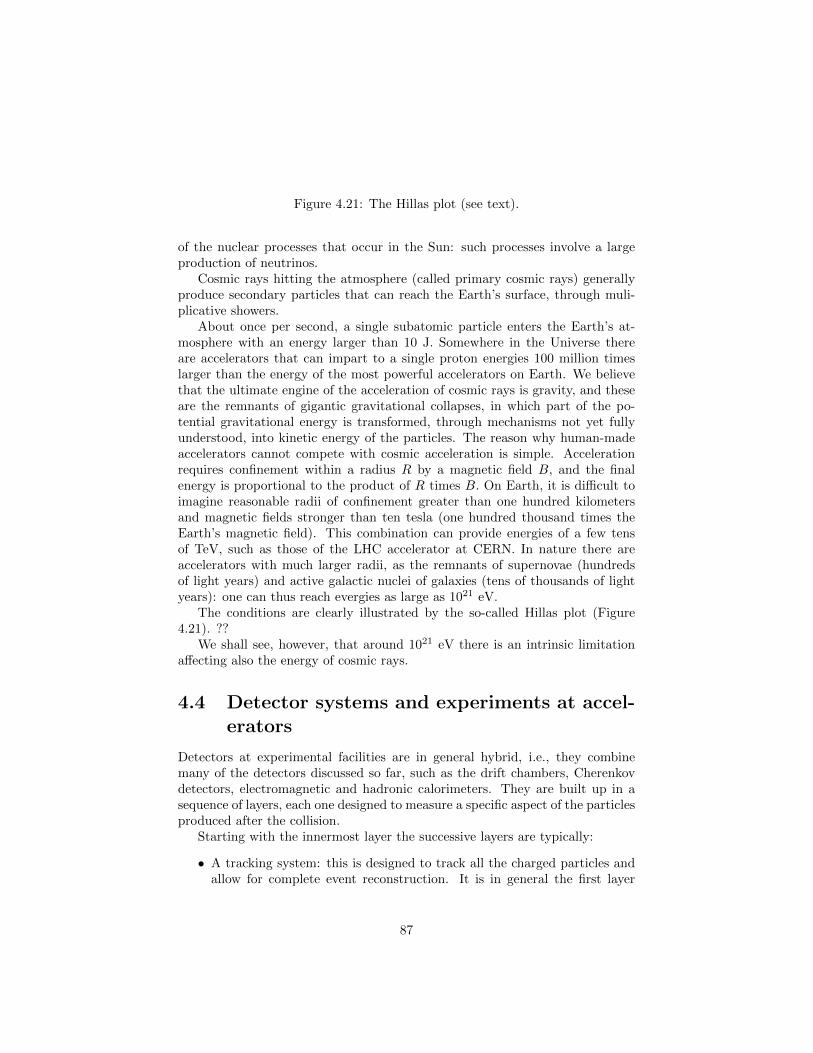
Figure 4.21: The Hillas plot (see text).

of the nuclear processes that occur in the Sun: such processes involve a largeproduction of neutrinos.

Cosmic rays hitting the atmosphere (called primary cosmic rays) generallyproduce secondary particles that can reach the Earth’s surface, through muli-plicative showers.

About once per second, a single subatomic particle enters the Earth’s at-mosphere with an energy larger than 10 J. Somewhere in the Universe thereare accelerators that can impart to a single proton energies 100 million timeslarger than the energy of the most powerful accelerators on Earth. We believethat the ultimate engine of the acceleration of cosmic rays is gravity, and theseare the remnants of gigantic gravitational collapses, in which part of the po-tential gravitational energy is transformed, through mechanisms not yet fullyunderstood, into kinetic energy of the particles. The reason why human-madeaccelerators cannot compete with cosmic acceleration is simple. Accelerationrequires confinement within a radius R by a magnetic field B, and the finalenergy is proportional to the product of R times B. On Earth, it is difficult toimagine reasonable radii of confinement greater than one hundred kilometersand magnetic fields stronger than ten tesla (one hundred thousand times theEarth’s magnetic field). This combination can provide energies of a few tensof TeV, such as those of the LHC accelerator at CERN. In nature there areaccelerators with much larger radii, as the remnants of supernovae (hundredsof light years) and active galactic nuclei of galaxies (tens of thousands of lightyears): one can thus reach evergies as large as 1021 eV.

The conditions are clearly illustrated by the so-called Hillas plot (Figure4.21). ??

We shall see, however, that around 1021 eV there is an intrinsic limitationaffecting also the energy of cosmic rays.

4.4 Detector systems and experiments at accel-erators

Detectors at experimental facilities are in general hybrid, i.e., they combinemany of the detectors discussed so far, such as the drift chambers, Cherenkovdetectors, electromagnetic and hadronic calorimeters. They are built up in asequence of layers, each one designed to measure a specific aspect of the particlesproduced after the collision.

Starting with the innermost layer the successive layers are typically:

• A tracking system: this is designed to track all the charged particles andallow for complete event reconstruction. It is in general the first layer

87

crossed by the particles, in such a way that their proporties have non yetbeen deteriorated by the interaction with the material of the detector. Itshould have as little material as possible, so to preserve the particles forthe subsequent layer.

• A layer devoted to electromagnetic calorimetry.

• A layer devoted to hadronic calorimetry.

• A layer of muon tracking chambers: any particle releasing signal on thesetracking detectors (often drift chambers) has necessarily travelled throughall the other layers and is very likely a muon6.

The particle species can be identified by energy loss, curvature in magneticfield and Cherenkov radiation. However, the search for the identity of a particlecan be significantly narrowed down by simply examining which parts of thedetector it deposits energy in:

• Photons leave no tracks in the tracking detectors (unless they undergo pairproduction) but produce a shower in the electromagnetic calorimeter.

• Electrons and positrons leave a track in the tracking detectors and producea shower in the electromagnetic calorimeter.

• Muons leave tracks in all the detectors (likely as a mip in the calorimeters).

• Long-lived charged hadrons (protons for example) leave tracks in all thedetectors up to the hadronic calorimeter where they shower and depositall their energy.

• Neutrinos are identified by missing energy-momentum when the relevantconservation law is applied to the event.

The signatures are summarized in Figure 4.22.

4.4.1 Examples of detectors for fixed-target experiments

In a fixed target experiment, relativistic effects make the interaction productsto be highly collimated. In such experiments then, in order to enhance the pos-sibility of detection in the small-xT (xT = pT /

√s, where pT is the momentum

component perpendicular to the beam direction), different stages are separatedby magnets opening up the charged particles in the final state (lever arms).

The first detectors along the beam line should be non-destructive; at the endof the bem line, one can have calorimeters. An example is given in the following.

88

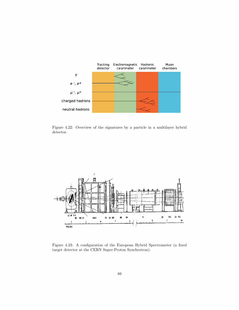
Figure 4.22: Overview of the signatures by a particle in a multilayer hybriddetector.

Figure 4.23: A configuration of the European Hybrid Spectrometer (a fixedtarget detector at the CERN Super-Proton Synchrotron).

89

The European Hybrid Spectrometer at the SPS

The European Hybrid Spectrometer EHS has been operational during the years1970s and the beginning of the 1980s at the North Area of CERN, where beamsof protons were extracted from the SPS accelerator at energies of 300 GeV-400 GeV. They might possibly generate seconday beams of charged pions ofshlightly smaller energies by a beam-dump and a velocity selector based onmagnetic field. EHS was a multi-stage detector serving different experiments(NA16, NA22, NA23, NA27). Here we describe a typical configuration; Figure4.23 shows a schematic drawing of the EHS set-up.

In the Figure, the beam particles come in from the left. Their direction isdetermined by the two small wire chambers U1 and U3. From the collision pointinside a rapid cycling bubble chamber(RCBC; LEBC for example) most of theproduced particles will enter the downstream part of the spectrometer. The fastones (typically with momentum p > 30 GeV/c) will go through the aperture ofthe magnet M2 to the so-called second lever arm.

The RCBC acts both as a target and as a vertex detector. If an event istriggered, stereopictures are taken with 3 cameras and recorded on film.

The momentum resolution of the secondary tracks depends on the number ofdetector element hits available for the fits. For low momentum tracks, typicallyp < 3 GeV/c, length and direction of the momentum vector at the collision-point can be well determined from RCBC. On the other hand, tracks withp < 3 GeV/c have a very good chance to enter the so-called 1st lever arm. Thisis defined by the group of 4 wire chambers W2, D1, D2 and D3 placed betweenthe two magnets M1 and M2.

Fast tracks, typically p > 50 GeV/c, have a good chance to go in additionthrough the gap of the magnet M2 and enter the 2nd lever arm, consisting ofthe 3 drift chambers D4, D5 and D6.

To detect gammas, two electromagnetic calorimeters are used in EHS, theintermediate gamma detector (IGD) and the forward gamma detector (FGD).IGD is placed before the magnet M2. It has a central hole to allow fast particlesto pass into the second lever arm. FGD covers this hole at the end of thespectrometer. The IGD has been designed to measure both position and energyof a shower in a two-dimensional matrix of lead-glass counters 5cm × 5cm insize, each of them connected to a PMT. The FGD consists of three separatesections. The first section is the converter, a lead glass wall, to initiate theelectromagnetic shower .The second section, the position detector, is a three-plane scintillator hodoscope with a finger width of 1.5 cm. The third section isthe absorber, a lead-glass matrix deep enough (60 rad. length) to totally absorbshowers up to the highest available energies. For both calorimeters, the relativeaccuracy on energy reconstruction was ∆E/E ' 0.1/

√E ⊕ 0.02.

6Neutrinos have extremely low interaction cross sections. Most probably they cross alsothe muon chambers without leaving any signal.

90

4.4.2 Examples of detectors for colliders

The modern particle detectors in use today at colliders are as much as possiblehermetic detectors. They are designed to cover as much as possible of the solidangle around the interaction point (a limitation being given by the presence ofthe beam pipe). The typical detector consists of a cylindrical section coveringthe “barrel” region and two endcaps covering the “forward” regions.

In the standard coordinate system, the z axis is along the beam direction,the x axis points towards the centre of the ring, and the y axis points upwards.The polar angle to the z axis is called θ and the azimuthal angle around the zaxis is called φ; the radial coordinate is R =

√x2 + y2.

Frequently the polar angle is replaced by a coordinate called pseudorapidityη and defined as

η = ln

(tan

(θ

2

));

the region η ' 0 corresponds to θ ' π/2, and is called the central region.The detector has the typical onion-like structure described in the previous

section: a sequence of layers, the innermost being the most precise for tracking.The configuration of the endcaps is similar to that in a fixed-target experi-

ment except for the necessary presence of a beampipe, which makes it impossibleto detect particles at vert small polar angles, and entails the possible productionof secondary particles in the pipe wall.

We analyze three generations of collider detectors operating at the Euro-pean Organization for Particle Physics, CERN: UA1 at the SPS pp accelerator,DELPHI at the LEP e+e− accelerator, CMS at the LHC pp accelerator. Weshall see how much the technology developed and the required labour increased;the basic idea is anyway still in one of the prototype detectors, UA1.

UA1 at the SppS

The UA1 experiment, named as the first experiment in the CERN UndergroundArea (UA), was a high-energy physics experiment running at CERN’s SppS(Super-proton-antiproton-Synchrotron) accelerator-collider from 1981 till 1993.The discovery of the W and Z bosons, mediators of the weak interaction, bythis experiment in 1983, led to the Nobel Prize for physics to Carlo Rubbia andSimon van der Meer in 1984 (the motivation of the prize being more relatedto the development of the collider technology). The SppS was colliding protonsand antiprotons at a typical c.m. energy of 540 GeV; 3 bunches of protonsand 3 bunches of antiprotons, 1011 particles per bunch, were colliding, and theluminosity was about 5× 1027 cm−2/s (5 inverse millibarn per second).

UA1 was a huge and complex detector for its day, and it was and still is theprototype of collider detectors. The collaboration constructing and managingthe detector included approximately 130 scientists from all around the world.

UA1 was a general-purpose detector. The central tracking chamber was anassembly of 6 drift chambers 5.8 m long and 2.3 m in diameter. It recorded thetracks of charged particles curving in a 0.7 T magnetic field, measuring their

91

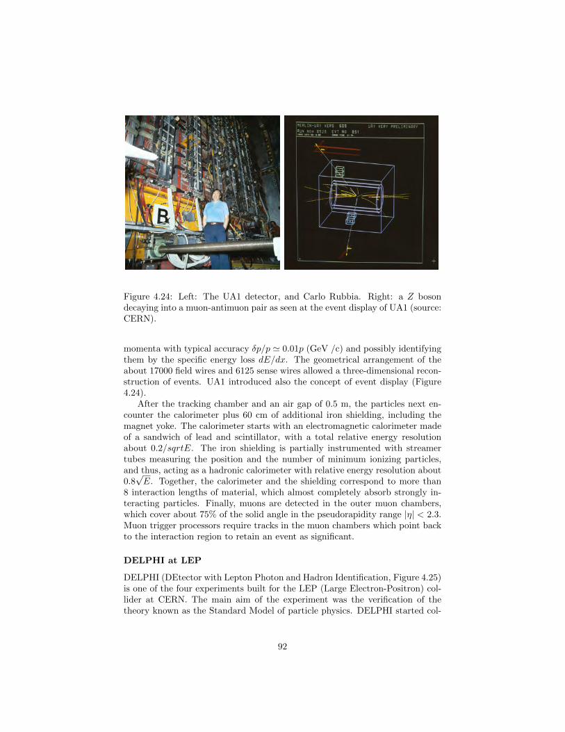
Figure 4.24: Left: The UA1 detector, and Carlo Rubbia. Right: a Z bosondecaying into a muon-antimuon pair as seen at the event display of UA1 (source:CERN).

momenta with typical accuracy δp/p ' 0.01p (GeV /c) and possibly identifyingthem by the specific energy loss dE/dx. The geometrical arrangement of theabout 17000 field wires and 6125 sense wires allowed a three-dimensional recon-struction of events. UA1 introduced also the concept of event display (Figure4.24).

After the tracking chamber and an air gap of 0.5 m, the particles next en-counter the calorimeter plus 60 cm of additional iron shielding, including themagnet yoke. The calorimeter starts with an electromagnetic calorimeter madeof a sandwich of lead and scintillator, with a total relative energy resolutionabout 0.2/sqrtE. The iron shielding is partially instrumented with streamertubes measuring the position and the number of minimum ionizing particles,and thus, acting as a hadronic calorimeter with relative energy resolution about0.8√E. Together, the calorimeter and the shielding correspond to more than

8 interaction lengths of material, which almost completely absorb strongly in-teracting particles. Finally, muons are detected in the outer muon chambers,which cover about 75% of the solid angle in the pseudorapidity range |η| < 2.3.Muon trigger processors require tracks in the muon chambers which point backto the interaction region to retain an event as significant.

DELPHI at LEP

DELPHI (DEtector with Lepton Photon and Hadron Identification, Figure 4.25)is one of the four experiments built for the LEP (Large Electron-Positron) col-lider at CERN. The main aim of the experiment was the verification of thetheory known as the Standard Model of particle physics. DELPHI started col-

92

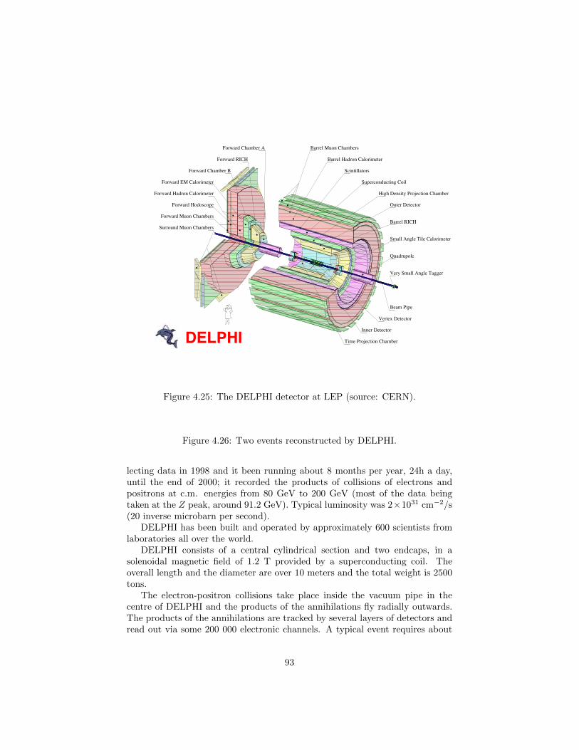
DELPHIVertex Detector

Inner Detector

Time Projection Chamber

Small Angle Tile Calorimeter

Very Small Angle Tagger

Beam Pipe

Quadrupole

Barrel RICH

Outer Detector

High Density Projection Chamber

Superconducting Coil

Scintillators

Barrel Hadron Calorimeter

Barrel Muon ChambersForward Chamber A

Forward RICH

Forward Chamber B

Forward EM Calorimeter

Forward Hadron Calorimeter

Forward Hodoscope

Forward Muon Chambers

Surround Muon Chambers

Figure 4.25: The DELPHI detector at LEP (source: CERN).

Figure 4.26: Two events reconstructed by DELPHI.

lecting data in 1998 and it been running about 8 months per year, 24h a day,until the end of 2000; it recorded the products of collisions of electrons andpositrons at c.m. energies from 80 GeV to 200 GeV (most of the data beingtaken at the Z peak, around 91.2 GeV). Typical luminosity was 2×1031 cm−2/s(20 inverse microbarn per second).

DELPHI has been built and operated by approximately 600 scientists fromlaboratories all over the world.

DELPHI consists of a central cylindrical section and two endcaps, in asolenoidal magnetic field of 1.2 T provided by a superconducting coil. Theoverall length and the diameter are over 10 meters and the total weight is 2500tons.

The electron-positron collisions take place inside the vacuum pipe in thecentre of DELPHI and the products of the annihilations fly radially outwards.The products of the annihilations are tracked by several layers of detectors andread out via some 200 000 electronic channels. A typical event requires about

93

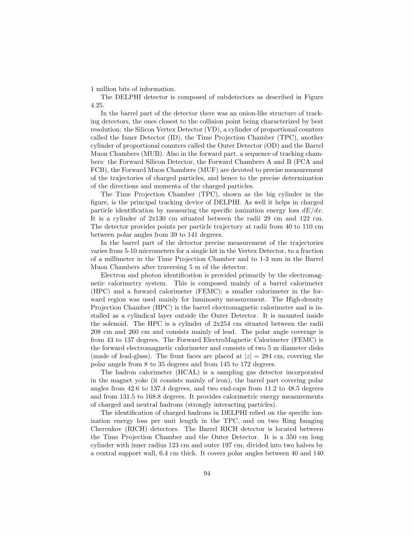
1 million bits of information.The DELPHI detector is composed of subdetectors as described in Figure

4.25.In the barrel part of the detector there was an onion-like structure of track-

ing detectors, the ones closest to the collision point being characterized by bestresolution: the Silicon Vertex Detector (VD), a cylinder of proportional counterscalled the Inner Detector (ID), the Time Projection Chamber (TPC), anothercylinder of proportional counters called the Outer Detector (OD) and the BarrelMuon Chambers (MUB). Also in the forward part, a sequence of tracking cham-bers: the Forward Silicon Detector, the Forward Chambers A and B (FCA andFCB), the Forward Muon Chambers (MUF) are devoted to precise measurementof the trajectories of charged particles, and hence to the precise determinationof the directions and momenta of the charged particles.

The Time Projection Chamber (TPC), shown as the big cylinder in thefigure, is the principal tracking device of DELPHI. As well it helps in chargedparticle identification by measuring the specific ionization energy loss dE/dx.It is a cylinder of 2x130 cm situated between the radii 29 cm and 122 cm.The detector provides points per particle trajectory at radii from 40 to 110 cmbetween polar angles from 39 to 141 degrees.

In the barrel part of the detector precise measurement of the trajectoriesvaries from 5-10 micrometers for a single hit in the Vertex Detector, to a fractionof a millimeter in the Time Projection Chamber and to 1-3 mm in the BarrelMuon Chambers after traversing 5 m of the detector.

Electron and photon identification is provided primarily by the electromag-netic calorimetry system. This is composed mainly of a barrel calorimeter(HPC) and a forward calorimeter (FEMC); a smaller calorimeter in the for-ward region was used mainly for luminosity measurement. The High-densityProjection Chamber (HPC) is the barrel electromagnetic calorimeter and is in-stalled as a cylindical layer outside the Outer Detector. It is mounted insidethe solenoid. The HPC is a cylinder of 2x254 cm situated between the radii208 cm and 260 cm and consists mainly of lead. The polar angle coverage isfrom 43 to 137 degrees. The Forward ElectroMagnetic Calorimeter (FEMC) isthe forward electromagnetic calorimeter and consists of two 5 m diameter disks(made of lead-glass). The front faces are placed at |z| = 284 cm, covering thepolar angels from 8 to 35 degrees and from 145 to 172 degrees.

The hadron calorimeter (HCAL) is a sampling gas detector incorporatedin the magnet yoke (it consists mainly of iron), the barrel part covering polarangles from 42.6 to 137.4 degrees, and two end-caps from 11.2 to 48.5 degreesand from 131.5 to 168.8 degrees. It provides calorimetric energy measurementsof charged and neutral hadrons (strongly interacting particles).

The identification of charged hadrons in DELPHI relied on the specific ion-ization energy loss per unit length in the TPC, and on two Ring ImagingCherenkov (RICH) detectors. The Barrel RICH detector is located betweenthe Time Projection Chamber and the Outer Detector. It is a 350 cm longcylinder with inner radius 123 cm and outer 197 cm, divided into two halves bya central support wall, 6.4 cm thick. It covers polar angles between 40 and 140

94

Table 4.4: Summary of the performance of DELPHI.

Figure 4.27: The CMS detector at LHC (source: CERN).

degrees. The Forward RICH Detector is located between 1.7 m < |z| < 2.7 mand covers polar angles between 15 and 35 degrees.

The overall performance of the DELPHI detector is summarized in Table4.4; two reconstructed events are shown in Figure 4.26.

CMS at LHC

The Compact Muon Solenoid (CMS) experiment is one of two large general-purpose particle physics detectors built on the proton-proton Large HadronCollider (LHC) at CERN. Approximately 3000 scientists, representing 183 re-search institutes and 38 countries, form the CMS collaboration who built andnow since 2008 operate the detector. The detector is shown in Figure 4.27.Proton-proton collisions at c.m. energies of 8 TeV are recorded; typical lumi-nosity is 7× 1034 cm−2/s (70 inverse nanobarn per second).

As customary for collider detectors, CMS in structured in layers.Layer 1 is devoted to tracking. Immediately around the interaction point

the inner silicon tracker serves to identify the tracks of individual particles

95

and match them to the vertices from which they originated. The curvatureof charged particle tracks in the magnetic field allows their charge and momen-tum to be measured. The CMS silicon tracker consists of 13 layers in the centralregion and 14 layers in the endcaps. The innermost three layers (up to 11 cmradius) consist of 100× 150 µm pixels, 66 million in total. The next four layers(up to 55 cm radius) consist of silicon strips. There are 9.6 million strip channelsin total. This part of the detector is the world’s largest silicon detector; it has205 m2 of silicon sensors (approximately the area of a tennis court) comprising76 million channels.

Layer 2 is devoted to Electromagnetic Calorimetry. The ElectromagneticCalorimeter (ECAL) is constructed from crystals of lead tungstate, PbWO4.;this is an extremely dense but optically clear material. It has a radiation lengthof 0.89 cm, and has a rapid light yield, with 80% of light yield within one crossingtime (25 ns). The light yield is of about 30 photons per MeV of incident energy.The crystals used have a front size of 22 mm × 22 mm and a depth of 23 cm.They are set in a matrix of carbon fibre to keep them optically isolated, andbacked by silicon avalanche photodiodes for readout. The barrel region consistsof about 60 thousand crystals, with a further about 7 thousand in each of theendcaps.

Layer 3 is devoted to Hadronic Calorimetry. The Hadronic Calorimeter(HCAL) consists of layers of dense material (brass or steel) interleaved withtiles of plastic scintillators, read out via wavelength-shifting fibres by hybridphotodiodes. This combination was determined to allow the maximum amountof absorbing material inside of the magnet coil.

Layer 4 is the magnet. It is 13 m long and 6 m in diameter, and it is arefrigerated superconducting niobium-titanium coil providing a solenoidal fieldof 3.8 T (the current being about 18000 A, giving a total stored energy of about2.5 GJ, equivalent to about 500 kg of TNT: there are dump circuits to safelydissipate this energy should the magnet quench).

Layer 5 is occupied by the muon detectors and the return yoke. To identifymuons and measure their momenta, CMS uses mostly drift tubes and RPCs.The drift tubes are used for precise trajectory measurements in the central barrelregion. The RPCs provide a fast signal when a muon passes through the muondetector.

To have a good chance of producing a rare particle, such as a Higgs boson, avery large number of collisions is required. Most collision events in the detectordo not produce interesting effects. The amount of raw data from each crossing isapproximately 1 megabyte, which at the 40 MHz crossing rate would result in 40terabytes of data a second, an amount that the experiment cannot hope to storeor process properly. The trigger system reduces the rate of interesting eventsdown to a manageable 100 per second. To accomplish this, a series of “trigger”stages are employed. All the data from each crossing are held in buffers withinthe detector while a small amount of key information is used to perform a fast,approximate calculation to identify features of interest such as high energy jets,muons or missing energy. This “Level 1” calculation is completed in around 1µs, and the event rate is reduced by a factor of about thousand down to 50 kHz.

96

Table 4.5: Summary of the performance of CMS.

All these calculations are done on fast, custom hardware using reprogrammablefield-programmable gate arrays (FPGA). If an event is passed by the Level 1trigger, all the data still buffered in the detector are sent over fibre-optic linksto the “High Level” trigger, which is software (mainly written in C++) runningon ordinary computer servers. The lower event rate in the High Level triggerallows time for a much more detailed analysis of the event to be done than inthe Level 1 trigger. The High Level trigger reduces the event rate by a furtherfactor of about a thousand down to around 100 events per second.

The overall performance of the CMS detector is summarized in Table 4.5.ADD events, and ATLAS ???Something on pile-up ??

97