particle detection with drift chambersparticle acceleration and detection springer.com the series...
TRANSCRIPT
Particle Detection with Drift Chambers

Particle Acceleration and Detectionspringer.com
The series Particle Acceleration and Detection is devoted to monograph texts dealingwith all aspects of particle acceleration and detection research and advanced teach-ing. The scope also includes topics such as beam physics and instrumentation as wellas applications. Presentations should strongly emphasize the underlying physical andengineering sciences. Of particular interest are
• contributions which relate fundamental research to new applications beyondthe immediate realm of the original field of research
• contributions which connect fundamental research in the aforementioned fieldsto fundamental research in related physical or engineering sciences
• concise accounts of newly emerging important topics that are embedded in abroader framework in order to provide quick but readable access of very newmaterial to a larger audience
The books forming this collection will be of importance for graduate students andactive researchers alike.
Series Editors:
Professor Alexander ChaoSLAC2575 Sand Hill RoadMenlo Park, CA 94025USA
Professor Christian W. FabjanCERNPPE Division1211 Genève 23Switzerland
Professor Rolf-Dieter HeuerDESYGebäude 1d/2522603 HamburgGermany
Professor Takahiko KondoKEKBuilding No. 3, Room 3191-1 Oho, 1-2 1-2 Tsukuba1-3 1-3 Ibaraki 305Japan
Professor Francesco RuggieroCERNSL Division1211 Genève 23Switzerland

Walter Blum · Werner Riegler · Luigi Rolandi
Particle Detectionwith Drift Chambers
123

Professor Walter Blum Doctor Werner RieglerMPI fur Physik CERNWerner-Heisenberg-Institut 1211 Geneve 23Fohringer Ring 6 Switzerland80805 Munchen [email protected]@cern.ch
Professor Luigi RolandiCERN1211 Geneve [email protected]
ISBN: 978-3-540-76683-4 e-ISBN: 978-3-540-76684-1
Library of Congress Control Number: 2007940836
c© 2008 Springer-Verlag Berlin Heidelberg
This work is subject to copyright. All rights are reserved, whether the whole or part of the material isconcerned, specifically the rights of translation, reprinting, reuse of illustrations, recitation, broadcasting,reproduction on microfilm or in any other way, and storage in data banks. Duplication of this publicationor parts thereof is permitted only under the provisions of the German Copyright Law of September 9,1965, in its current version, and permission for use must always be obtained from Springer. Violations areliable to prosecution under the German Copyright Law.
The use of general descriptive names, registered names, trademarks, etc. in this publication does not imply,even in the absence of a specific statement, that such names are exempt from the relevant protective lawsand regulations and therefore free for general use.
Cover design: WMXDesign GmbH
Printed on acid-free paper
9 8 7 6 5 4 3 2 1
springer.com
Preface to the First Edition
A drift chamber is an apparatus for measuring the space coordinates of the trajectoryof a charged particle. This is achieved by detecting the ionization electrons producedby the charged particle in the gas of the chamber and by measuring their drift timesand arrival positions on sensitive electrodes.
When the multiwire proportional chamber, or ‘Charpak chamber’ as we used tocall it, was introduced in 1968, its authors had already noted that the time of a signalcould be useful for a coordinate determination, and first studies with a drift cham-ber were made by Bressani, Charpak, Rahm and Zupancic in 1969. When the firstoperational drift-chamber system with electric circuitry and readout was built byWalenta, Heintze and Schurlein in 1971, a new instrument for particle experimentshad appeared. A broad study of the behaviour of drifting electrons in gases began inlaboratories where there was interest in the detection of particles.
Diffusion and drift of electrons and ions in gases were at that time well-establishedsubjects in their own right. The study of the influence of magnetic fields on theseprocesses was completed in the 1930s and all fundamental equations were con-tained in the article by W.P. Allis in the Encyclopedia of Physics [ALL 56]. Itdid not take very long until the particle physicists learnt to apply the methods ofthe Maxwell–Boltzmann equations and of the electron-swarm experiments that hadbeen developed for the study of atomic properties. The article by Palladino andSadoulet [PAL 75] recorded some of these methods for use with particle-physicsinstruments.
F. Sauli gave an academic training course at CERN in 1975/76, in order to informa growing number of users of the new devices. He published lecture notes [SAU 77],which were a major source of information for particle physicists who began to workwith drift chambers.
When the authors of this book began to think about a large drift chamber forthe ALEPH experiment, we realized that there was no single text to introduce us tothose questions about drift chambers that would allow us to determine their ultimatelimits of performance. We wanted to have a text, not on the technical details, buton the fundamental processes, so that a judgement about the various alternativesfor building a drift chamber would be on solid ground. We needed some insight
v
vi Preface to the First Edition
into the consequences of different geometries and how to distinguish between thebehaviour of different gases, not so much a complete table of their properties. Wewanted to understand on what trajectories the ionization electrons would drift to theproportional wires and to what extent the tracks would change their shape.
Paths to the literature were also required – just a few essential ones – so that anentry point to every important subject existed; they would not have to be a compre-hensive review of ‘everything’.
In some sense we have written the book that we wanted at that time. The textalso contains a number of calculations that we made concerning the statistics ofionization and the fundamental limits of measuring accuracy that result from it,geometrical fits to curved tracks, and electrostatics of wire grids and field cages.Several experiments that we undertook during the construction time of the ALEPHexperiment found their way into the book; they deal mainly with the drift and diffu-sion of electrons in gases under various field conditions, but also with the statisticsof the ionization and amplification processes.
The book is nonetheless incomplete in some respects. We are aware that it lacksa chapter on electronic signal processing. Also some of the calculations are not yetbacked up in detail by measurements as they will eventually have to be. Especiallythe parameter Neff of the ionization process which governs the achievable accuracyshould be accurately known and supported by measurements with interesting gases.We hope that workers in this field will direct their efforts to such questions. Wewould welcome comments about any other important omissions.
It was our intention to make the book readable for students who are interestedin particle detectors. Therefore, we usually tried to explain in some detail the ar-guments that lead up to a final result. One may say that the book represents a crossbetween a monograph and an advanced textbook. Those who require a compendiouscatalogue of existing or proposed drift chambers may find useful the proceedings ofthe triannual Vienna Wire Chamber Conferences [VIE] or of the annual IEEE Sym-posia on Instrumentation for Nuclear Science [IEE].
Parts of the material have been presented in summer schools and guest lectures,and we thank H.D. Dahmen (Herbstschule Maria Laach), E. Fernandez (UniversitaAutonoma, Barcelona) and L. Bertocchi (ICTP, Trieste) for their hospitality.
We thank our colleagues from the ALEPH TPC group, and especially J. Mayand F. Ragusa, for many stimulating discussions on the issues of this book. We arealso obliged to H. Spitzer (Hamburg) who read and commented on an early versionof the manuscript. Special thanks are extended to Mrs. Heininger in Munich whoproduced most of the drawings.
Geneva W. Blum1 April 1993 L. Rolandi

Preface to the Second Edition
The first edition has continuously served many students and researchers in the field.Now we have enlarged and improved the book, essentially in three ways: (1) Thechapter on electronic signal processing was added, and (2) the chapter on the cre-ation of the signal was rewritten and based on the principle of current induction.This was made possible because our team was complemented with a new youngco-author (W.R.). (3) Also there are various modernizations throughout the book in-cluding some of the recent chambers capable to measure tracks at very high fluencesthat one could not imagine 15 years ago. Four of the chapters were left untouched.The development of drift chambers in the last 15 years was driven by the idea thattheir performance should be pushed towards the limits of the laws of physics. Theconcept of the book matches very well this trend because it is the basic principlesof drift chambers rather than their technical design solutions that are in focus. Themost modern design solutions, among them the ones developed for the experimentsof the Large Hadron Collider, can be found e.g. in the proceedings of the IEEESymposia [IEE] and of the Vienna Wire Chamber Conferences [VIE].
During the last two decades, the development and optimization of drift cham-bers has increasingly relied on simulation programs, which in some sense ’encode’the physics processes described in this book. The program GARFIELD, written byRob Veenhof, is the most widely used tool for drift chamber simulation. It allowscalculation of electric fields, electron and ion drift lines, induced signals, electro-static wire displacements and many more features of drift chambers. For calculationof the primary ionization of fast particles in gases, the program HEED, written byIgor Smirnov, is widely used. A very popular program for calculation of electrontransport properties in different gas mixtures is the program MAGBOLTZ, writ-ten by Steve Biagi. MAGBOLTZ and HEED are directly interfaced to GARFIELD,which therefore allows a complete simulation of the drift chamber processes, fromthe passage of the charged particle to the detector output signal. Clearly a thoroughunderstanding of drift chambers, which is subject of this book, is a necessary pre-condition for efficient use of these simulation programs.
Despite the development of the fine grained silicon detectors which now out-perform the wire chambers near the interaction point, the large detector volumes
vii
viii Preface to the Second Edition
surrounding modern experiments have to rely on drift chambers because of theirsimplicity and also because their measurement accuracy in relation to their size isbetter than it is in any other instrument. Time Projection Chambers with electrondrift lengths up to 2.5 m are the most important tools for studying heavy ion col-lisions, because of their very low material budget, channel number economy andparticle identification capabilities. TPCs are also studied as principle detectors forfuture electron colliders. 36 years after the first working drift chamber, these instru-ments are still going strong.
Geneva W. BlumApril 2008 W. Riegler
L. Rolandi
References
[ALL 56] W.P. Allis, Motions of ions and electrons, in Handbuch der Physik, ed. by S. Flugge(Springer, Berlin 1956) Vol. XXI, p. 383
[IEE] The symposia are usually held in the fall of every year and are published in consec-utive volumes of the IEEE Transactions in Nuclear Science in the first issue of thefollowing year
[PAL 75] V. Palladino and B. Sadoulet, Application of classical theory of electrons in gases todrift proportional chambers, Nucl. Instrum. Methods 128, 323 (1975)
[SAU 77] F. Sauli, Principles of operation of multiwire proportional and drift chambers, Lec-tures given in the academic training programme of CERN 1975–76 (CERN 77-09,Geneva 1977), in Experimental Techniques in High Energy Physics, ed. by T. Ferbel(Addison-Wesley, Menlo Park 1987)
[VIE] The Vienna Wire Chamber Conferences were held in February of the years 1978,1980, 1983, 1986, 1989, 1992, 1995, 1998, 2001, 2004, 2007, and they were publishedmostly the same years in Nuclear Instruments and Methods in the following volumes:135, 176, 217, A 252, A 283, A 323, A 367, A 419, A 478, A 535. Since 2001 theyare called Vienna Conference on Instrumentation.

Contents
1 Gas Ionization by Charged Particles and by Laser Rays . . . . . . . . . . . . 11.1 Gas Ionization by Fast Charged Particles . . . . . . . . . . . . . . . . . . . . . . . 1
1.1.1 Ionizing Collisions . . . . . . . . . . . . . . . . . . . . . . . . . . . . . . . . . . . 11.1.2 Different Ionization Mechanisms . . . . . . . . . . . . . . . . . . . . . . . 31.1.3 Average Energy Required to Produce One Ion Pair . . . . . . . . 41.1.4 The Range of Primary Electrons . . . . . . . . . . . . . . . . . . . . . . . . 71.1.5 The Differential Cross-section dσ/dE . . . . . . . . . . . . . . . . . . . 7
1.2 Calculation of Energy Loss . . . . . . . . . . . . . . . . . . . . . . . . . . . . . . . . . . 91.2.1 Force on a Charge Travelling Through a Polarizable Medium 91.2.2 The Photo-Absorption Ionization Model . . . . . . . . . . . . . . . . . 111.2.3 Behaviour for Large E . . . . . . . . . . . . . . . . . . . . . . . . . . . . . . . . 151.2.4 Cluster-Size Distribution . . . . . . . . . . . . . . . . . . . . . . . . . . . . . . 151.2.5 Ionization Distribution on a Given Track Length . . . . . . . . . . 161.2.6 Velocity Dependence of the Energy Loss . . . . . . . . . . . . . . . . 241.2.7 The Bethe–Bloch Formula . . . . . . . . . . . . . . . . . . . . . . . . . . . . 291.2.8 Energy Deposited on a Track – Restricted Energy Loss . . . . 321.2.9 Localization of Charge Along the Track . . . . . . . . . . . . . . . . . 351.2.10 A Measurement of Neff . . . . . . . . . . . . . . . . . . . . . . . . . . . . . . . 37
1.3 Gas Ionization by Laser Rays . . . . . . . . . . . . . . . . . . . . . . . . . . . . . . . . 381.3.1 The nth Order Cross-Section Equivalent . . . . . . . . . . . . . . . . . 381.3.2 Rate Equations for Two-Photon Ionization . . . . . . . . . . . . . . . 391.3.3 Dependence of Laser Ionization on Wavelength . . . . . . . . . . . 421.3.4 Laser-Beam Optics . . . . . . . . . . . . . . . . . . . . . . . . . . . . . . . . . . . 44
References . . . . . . . . . . . . . . . . . . . . . . . . . . . . . . . . . . . . . . . . . . . . . . . . . . . . . 46
2 The Drift of Electrons and Ions in Gases . . . . . . . . . . . . . . . . . . . . . . . . . . 492.1 An Equation of Motion with Friction . . . . . . . . . . . . . . . . . . . . . . . . . . 49
2.1.1 Case of E Nearly Parallel to B . . . . . . . . . . . . . . . . . . . . . . . . . 522.1.2 Case of E Orthogonal to B . . . . . . . . . . . . . . . . . . . . . . . . . . . . 52
2.2 The Microscopic Picture . . . . . . . . . . . . . . . . . . . . . . . . . . . . . . . . . . . . . 532.2.1 Drift of Electrons . . . . . . . . . . . . . . . . . . . . . . . . . . . . . . . . . . . . 53
ix
x Contents
2.2.2 Drift of Ions . . . . . . . . . . . . . . . . . . . . . . . . . . . . . . . . . . . . . . . . 562.2.3 Inclusion of Magnetic Field . . . . . . . . . . . . . . . . . . . . . . . . . . . 642.2.4 Diffusion . . . . . . . . . . . . . . . . . . . . . . . . . . . . . . . . . . . . . . . . . . 672.2.5 Electric Anisotropy . . . . . . . . . . . . . . . . . . . . . . . . . . . . . . . . . . 702.2.6 Magnetic Anisotropy . . . . . . . . . . . . . . . . . . . . . . . . . . . . . . . . . 722.2.7 Electron Attachment . . . . . . . . . . . . . . . . . . . . . . . . . . . . . . . . . 75
2.3 Results from the Complete Microscopic Theory . . . . . . . . . . . . . . . . . 792.3.1 Distribution Function of Velocities . . . . . . . . . . . . . . . . . . . . . . 792.3.2 Drift . . . . . . . . . . . . . . . . . . . . . . . . . . . . . . . . . . . . . . . . . . . . . . . 812.3.3 Inclusion of Magnetic Field . . . . . . . . . . . . . . . . . . . . . . . . . . . 822.3.4 Diffusion . . . . . . . . . . . . . . . . . . . . . . . . . . . . . . . . . . . . . . . . . . . 83
2.4 Applications . . . . . . . . . . . . . . . . . . . . . . . . . . . . . . . . . . . . . . . . . . . . . . . 832.4.1 Determination of σ(ε) and λ(ε) from Drift Measurement . . 832.4.2 Example: Argon–Methane Mixture . . . . . . . . . . . . . . . . . . . . . 852.4.3 Experimental Check of the Universal Drift Velocity
for Large ωτ . . . . . . . . . . . . . . . . . . . . . . . . . . . . . . . . . . . . . . . . 882.4.4 A Measurement of Track Displacement as a Function
of Magnetic Field . . . . . . . . . . . . . . . . . . . . . . . . . . . . . . . . . . . . 892.4.5 A Measurement of the Magnetic Anisotropy of Diffusion . . . 892.4.6 Calculated and Measured Electron Drift Velocities
in Crossed Electric and Magnetic Fields . . . . . . . . . . . . . . . . . 92References . . . . . . . . . . . . . . . . . . . . . . . . . . . . . . . . . . . . . . . . . . . . . . . . . . . . . 94
3 Electrostatics of Tubes, Wire Grids and Field Cages . . . . . . . . . . . . . . . . 973.1 Perfect and Imperfect Drift Tubes . . . . . . . . . . . . . . . . . . . . . . . . . . . . . 98
3.1.1 Perfect Drift Tube . . . . . . . . . . . . . . . . . . . . . . . . . . . . . . . . . . . . 993.1.2 Displaced Wire . . . . . . . . . . . . . . . . . . . . . . . . . . . . . . . . . . . . . . 99
3.2 Wire Grids . . . . . . . . . . . . . . . . . . . . . . . . . . . . . . . . . . . . . . . . . . . . . . . . 1053.2.1 The Electric Field of an Ideal Grid of Wires Parallel
to a Conducting Plane . . . . . . . . . . . . . . . . . . . . . . . . . . . . . . . . 1053.2.2 Superposition of the Electric Fields of Several Grids
and of a High-Voltage Plane . . . . . . . . . . . . . . . . . . . . . . . . . . . 1083.2.3 Matching the Potential of the Zero Grid and of the
Electrodes of the Field Cage . . . . . . . . . . . . . . . . . . . . . . . . . . . 1103.3 An Ion Gate in the Drift Space . . . . . . . . . . . . . . . . . . . . . . . . . . . . . . . . 112
3.3.1 Calculation of Transparency . . . . . . . . . . . . . . . . . . . . . . . . . . . 1133.3.2 Setting of the Gating Grid Potential with Respect
to the Zero-Grid Potential . . . . . . . . . . . . . . . . . . . . . . . . . . . . . 1183.4 Field Cages . . . . . . . . . . . . . . . . . . . . . . . . . . . . . . . . . . . . . . . . . . . . . . . 118
3.4.1 The Difficulty of Free Dielectric Surfaces . . . . . . . . . . . . . . . . 1193.4.2 Irregularities in the Field Cage . . . . . . . . . . . . . . . . . . . . . . . . . 121
References . . . . . . . . . . . . . . . . . . . . . . . . . . . . . . . . . . . . . . . . . . . . . . . . . . . . . 124

Contents xi
4 Amplification of Ionization . . . . . . . . . . . . . . . . . . . . . . . . . . . . . . . . . . . . . . 1254.1 The Proportional Wire . . . . . . . . . . . . . . . . . . . . . . . . . . . . . . . . . . . . . . 1254.2 Beyond the Proportional Mode . . . . . . . . . . . . . . . . . . . . . . . . . . . . . . . 1284.3 Lateral Extent of the Avalanche . . . . . . . . . . . . . . . . . . . . . . . . . . . . . . . 1304.4 Amplification Factor (Gain) of the Proportional Wire . . . . . . . . . . . . . 132
4.4.1 The Diethorn Formula . . . . . . . . . . . . . . . . . . . . . . . . . . . . . . . . 1344.4.2 Dependence of the Gain on the Gas Density . . . . . . . . . . . . . . 1364.4.3 Measurement of the Gain Variation with Sense-Wire
Voltage and Gas Pressure . . . . . . . . . . . . . . . . . . . . . . . . . . . . . 1364.5 Local Variations of the Gain . . . . . . . . . . . . . . . . . . . . . . . . . . . . . . . . . . 138
4.5.1 Variation of the Gain Near the Edge of the Chamber . . . . . . . 1384.5.2 Local Variation of the Gain Owing to Mechanical
Imperfections . . . . . . . . . . . . . . . . . . . . . . . . . . . . . . . . . . . . . . . 1394.5.3 Gain Drop due to Space Charge . . . . . . . . . . . . . . . . . . . . . . . . 142
4.6 Statistical Fluctuation of the Gain . . . . . . . . . . . . . . . . . . . . . . . . . . . . . 1454.6.1 Distributions of Avalanches in Weak Fields . . . . . . . . . . . . . . 1454.6.2 Distributions of Avalanches in Electronegative Gases . . . . . . 1474.6.3 Distributions of Avalanches in Strong Homogeneous Fields . 1494.6.4 Distributions of Avalanches in Strong Non-uniform Fields . . 1514.6.5 The Effect of Avalanche Fluctuations on the Wire
Pulse Heights . . . . . . . . . . . . . . . . . . . . . . . . . . . . . . . . . . . . . . . 1514.6.6 A Measurement of Avalanche Fluctuations
Using Laser Tracks . . . . . . . . . . . . . . . . . . . . . . . . . . . . . . . . . . . 152References . . . . . . . . . . . . . . . . . . . . . . . . . . . . . . . . . . . . . . . . . . . . . . . . . . . . . 154
5 Creation of the Signal . . . . . . . . . . . . . . . . . . . . . . . . . . . . . . . . . . . . . . . . . . 1575.1 The Principle of Signal Induction by Moving Charges . . . . . . . . . . . . 1575.2 Capacitance Matrix, Reciprocity Theorem . . . . . . . . . . . . . . . . . . . . . . 1585.3 Signals Induced on Grounded Electrodes, Ramo’s Theorem . . . . . . . 1605.4 Total Induced Charge and Sum of Induced Signals . . . . . . . . . . . . . . . 1615.5 Induced Signals in a Drift Tube . . . . . . . . . . . . . . . . . . . . . . . . . . . . . . . 1635.6 Signals Induced on Electrodes Connected with Impedance Elements 165
5.6.1 Application to a Drift Tube and its Circuitry . . . . . . . . . . . . . . 1695.6.2 Alternative Methods for the Calculation of the Signal . . . . . . 171
5.7 Signals Induced in Multiwire Chambers . . . . . . . . . . . . . . . . . . . . . . . . 1725.7.1 Signals Induced on Wires . . . . . . . . . . . . . . . . . . . . . . . . . . . . . 1725.7.2 Signals Induced on Cathode Strips and Pads . . . . . . . . . . . . . . 176
References . . . . . . . . . . . . . . . . . . . . . . . . . . . . . . . . . . . . . . . . . . . . . . . . . . . . . 179
6 Electronics for Drift Chambers . . . . . . . . . . . . . . . . . . . . . . . . . . . . . . . . . . 1816.1 Linear Signal Processing . . . . . . . . . . . . . . . . . . . . . . . . . . . . . . . . . . . . 183
6.1.1 Laplace and Fourier Transforms . . . . . . . . . . . . . . . . . . . . . . . . 1836.1.2 Transfer Functions, Poles and Zeros, Delta Response . . . . . . 1856.1.3 CR, RC, Pole-zero and Zero-pole Filters . . . . . . . . . . . . . . . . . 1876.1.4 Cascading of Circuit Elements . . . . . . . . . . . . . . . . . . . . . . . . . 191

xii Contents
6.1.5 Amplifier Types, Bandwidth, Sensitivity, and BallisticDeficit . . . . . . . . . . . . . . . . . . . . . . . . . . . . . . . . . . . . . . . . . . . . . 192
6.2 Signal Shaping . . . . . . . . . . . . . . . . . . . . . . . . . . . . . . . . . . . . . . . . . . . . . 1946.2.1 Unipolar and Bipolar Signal Shaping . . . . . . . . . . . . . . . . . . . . 1956.2.2 Signal Tail Cancellation . . . . . . . . . . . . . . . . . . . . . . . . . . . . . . . 2006.2.3 Signal Pileup, Baseline Shift, and Baseline Fluctuations . . . . 2056.2.4 Input Circuit . . . . . . . . . . . . . . . . . . . . . . . . . . . . . . . . . . . . . . . . 211
6.3 Noise and Optimum Filters . . . . . . . . . . . . . . . . . . . . . . . . . . . . . . . . . . 2136.3.1 Noise Characterization . . . . . . . . . . . . . . . . . . . . . . . . . . . . . . . . 2146.3.2 Noise Sources . . . . . . . . . . . . . . . . . . . . . . . . . . . . . . . . . . . . . . . 2176.3.3 Noise in Wire Chambers . . . . . . . . . . . . . . . . . . . . . . . . . . . . . . 2256.3.4 A Universal Limit on the Signal-to-Noise Ratio . . . . . . . . . . . 231
6.4 Electronics for Charge Measurement . . . . . . . . . . . . . . . . . . . . . . . . . . 2346.5 Electronics for Time Measurement . . . . . . . . . . . . . . . . . . . . . . . . . . . . 235
6.5.1 Influence of Electronics Noise on Time Resolution . . . . . . . . 2376.5.2 Influence of Pulse-Height Fluctuations on Time Resolution . 2396.5.3 Influence of Electron Arrival Time Fluctuations
on Time Resolution . . . . . . . . . . . . . . . . . . . . . . . . . . . . . . . . . . 2416.6 Three Examples of Modern Drift Chamber Electronics . . . . . . . . . . . 246
6.6.1 The ASDBLR Front-end Electronics . . . . . . . . . . . . . . . . . . . . 2466.6.2 The ATLAS CSC Front-end Electronics . . . . . . . . . . . . . . . . . 2476.6.3 The PASA and ALTRO Electronics for the ALICE TPC . . . . 247
References . . . . . . . . . . . . . . . . . . . . . . . . . . . . . . . . . . . . . . . . . . . . . . . . . . . . . 248
7 Coordinate Measurement and Fundamental Limits of Accuracy . . . . . 2517.1 Methods of Coordinate Measurement . . . . . . . . . . . . . . . . . . . . . . . . . . 2517.2 Basic Formulae for a Single Wire . . . . . . . . . . . . . . . . . . . . . . . . . . . . . 253
7.2.1 Frequency Distribution of the Coordinates of a SingleElectron at the Entrance to the Wire Region . . . . . . . . . . . . . . 254
7.2.2 Frequency Distribution of the Arrival Time of a SingleElectron at the Entrance to the Wire Region . . . . . . . . . . . . . . 256
7.2.3 Influence of the Cluster Fluctuations on the Resolution –the Effective Number of Electrons . . . . . . . . . . . . . . . . . . . . . . 257
7.3 Accuracy in the Measurement of the Coordinate in or near the WireDirection . . . . . . . . . . . . . . . . . . . . . . . . . . . . . . . . . . . . . . . . . . . . . . . . . . 2617.3.1 Inclusion of a Magnetic Field Perpendicular to the Wire
Direction: the Wire E ××× B Effect . . . . . . . . . . . . . . . . . . . . . . . 2617.3.2 Case Study of the Explicit Dependence of the Resolution
on L and θ . . . . . . . . . . . . . . . . . . . . . . . . . . . . . . . . . . . . . . . . . . 2637.3.3 The General Situation – Contributions of Several Wires,
and the Angular Pad Effect . . . . . . . . . . . . . . . . . . . . . . . . . . . . 2647.3.4 Consequences of (7.33) for the Construction of TPCs . . . . . . 2687.3.5 A Measurement of the Angular Variation of the Accuracy . . 268
7.4 Accuracy in the Measurement of the Coordinatein the Drift Direction . . . . . . . . . . . . . . . . . . . . . . . . . . . . . . . . . . . . . . . . 270
Contents xiii
7.4.1 Inclusion of a Magnetic Field Parallel to the WireDirection: the Drift E×B Effect . . . . . . . . . . . . . . . . . . . . . . . 271
7.4.2 Average Arrival Time of Many Electrons . . . . . . . . . . . . . . . . 2727.4.3 Arrival Time of the Mth Electron . . . . . . . . . . . . . . . . . . . . . . . 2727.4.4 Variance of the Arrival Time of the Mth Electron:
Contribution of the Drift-Path Variations . . . . . . . . . . . . . . . . . 2737.4.5 Variance of the Arrival Time of the Mth Electron:
Contribution of the Diffusion . . . . . . . . . . . . . . . . . . . . . . . . . . 2757.5 Accuracy Limitation Owing to Wire Vibrations . . . . . . . . . . . . . . . . . 277
7.5.1 Linear Harmonic Oscillator Driven by Random Pulses . . . . . 2787.5.2 Wire Excited by Avalanche Ions . . . . . . . . . . . . . . . . . . . . . . . . 279
7.6 Accuracy Limitation Owing to Space Charge Fluctuations . . . . . . . . 281References . . . . . . . . . . . . . . . . . . . . . . . . . . . . . . . . . . . . . . . . . . . . . . . . . . . . . 288
8 Geometrical Track Parameters and Their Errors . . . . . . . . . . . . . . . . . . 2918.1 Linear Fit . . . . . . . . . . . . . . . . . . . . . . . . . . . . . . . . . . . . . . . . . . . . . . . . . 292
8.1.1 Case of Equal Spacing Between x0 and xN . . . . . . . . . . . . . . . 2938.2 Quadratic Fit . . . . . . . . . . . . . . . . . . . . . . . . . . . . . . . . . . . . . . . . . . . . . . 294
8.2.1 Error Calculation . . . . . . . . . . . . . . . . . . . . . . . . . . . . . . . . . . . . 2958.2.2 Origin at the Centre of the Track – Uniform
Spacing of Wires . . . . . . . . . . . . . . . . . . . . . . . . . . . . . . . . . . . . 2968.2.3 Sagitta . . . . . . . . . . . . . . . . . . . . . . . . . . . . . . . . . . . . . . . . . . . . . 2988.2.4 Covariance Matrix at an Arbitrary Point Along
the Track . . . . . . . . . . . . . . . . . . . . . . . . . . . . . . . . . . . . . . . . . . . 2998.2.5 Comparison Between the Linear and Quadratic Fits
in Special Cases . . . . . . . . . . . . . . . . . . . . . . . . . . . . . . . . . . . . . 3008.2.6 Optimal Spacing of Wires . . . . . . . . . . . . . . . . . . . . . . . . . . . . . 302
8.3 A Chamber and One Additional Measuring Point Outside . . . . . . . . . 3028.3.1 Comparison of the Accuracy in the Curvature Measurement 3048.3.2 Extrapolation to a Vertex . . . . . . . . . . . . . . . . . . . . . . . . . . . . . . 304
8.4 Limitations Due to Multiple Scattering . . . . . . . . . . . . . . . . . . . . . . . . . 3068.4.1 Basic Formulae . . . . . . . . . . . . . . . . . . . . . . . . . . . . . . . . . . . . . . 3068.4.2 Vertex Determination . . . . . . . . . . . . . . . . . . . . . . . . . . . . . . . . . 3098.4.3 Resolution of Curvature for Tracks Through
a Scattering Medium . . . . . . . . . . . . . . . . . . . . . . . . . . . . . . . . . 3108.5 Spectrometer Resolution . . . . . . . . . . . . . . . . . . . . . . . . . . . . . . . . . . . . . 311
8.5.1 Limit of Measurement Errors . . . . . . . . . . . . . . . . . . . . . . . . . . 3118.5.2 Limit of Multiple Scattering . . . . . . . . . . . . . . . . . . . . . . . . . . . 312
References . . . . . . . . . . . . . . . . . . . . . . . . . . . . . . . . . . . . . . . . . . . . . . . . . . . . . 313
9 Ion Gates . . . . . . . . . . . . . . . . . . . . . . . . . . . . . . . . . . . . . . . . . . . . . . . . . . . . . 3159.1 Reasons for the Use of Ion Gates . . . . . . . . . . . . . . . . . . . . . . . . . . . . . . 315
9.1.1 Electric Charge in the Drift Region . . . . . . . . . . . . . . . . . . . . . 3159.1.2 Ageing . . . . . . . . . . . . . . . . . . . . . . . . . . . . . . . . . . . . . . . . . . . . . 318
9.2 Survey of Field Configurations and Trigger Modes . . . . . . . . . . . . . . . 318

xiv Contents
9.2.1 Three Field Configurations . . . . . . . . . . . . . . . . . . . . . . . . . . . . 3189.2.2 Three Trigger Modes . . . . . . . . . . . . . . . . . . . . . . . . . . . . . . . . . 320
9.3 Transparency under Various Operating Conditions . . . . . . . . . . . . . . . 3209.3.1 Transparency of the Static Bipolar Gate . . . . . . . . . . . . . . . . . 3219.3.2 Average Transparency
of the Regularly Pulsed Bipolar Gate . . . . . . . . . . . . . . . . . . . . 3239.3.3 Transparency of the Static Bipolar Gate in a Transverse
Magnetic Field . . . . . . . . . . . . . . . . . . . . . . . . . . . . . . . . . . . . . . 326References . . . . . . . . . . . . . . . . . . . . . . . . . . . . . . . . . . . . . . . . . . . . . . . . . . . . . 329
10 Particle Identification by Measurement of Ionization . . . . . . . . . . . . . . . 33110.1 Principles . . . . . . . . . . . . . . . . . . . . . . . . . . . . . . . . . . . . . . . . . . . . . . . . . 33110.2 Shape of the Ionization Curve . . . . . . . . . . . . . . . . . . . . . . . . . . . . . . . . 33410.3 Statistical Treatment of the n Ionization Samples
of One Track . . . . . . . . . . . . . . . . . . . . . . . . . . . . . . . . . . . . . . . . . . . . . . 33710.4 Accuracy of the Ionization Measurement . . . . . . . . . . . . . . . . . . . . . . . 339
10.4.1 Variation with n and x . . . . . . . . . . . . . . . . . . . . . . . . . . . . . . . . 33910.4.2 Variation with the Particle Velocity . . . . . . . . . . . . . . . . . . . . . 34010.4.3 Variation with the Gas . . . . . . . . . . . . . . . . . . . . . . . . . . . . . . . . 341
10.5 Particle Separation . . . . . . . . . . . . . . . . . . . . . . . . . . . . . . . . . . . . . . . . . 34410.6 Cluster Counting . . . . . . . . . . . . . . . . . . . . . . . . . . . . . . . . . . . . . . . . . . . 34510.7 Ionization Measurement in Practice . . . . . . . . . . . . . . . . . . . . . . . . . . . 347
10.7.1 Track-Independent Corrections . . . . . . . . . . . . . . . . . . . . . . . . . 34710.7.2 Track-Dependent Corrections . . . . . . . . . . . . . . . . . . . . . . . . . . 348
10.8 Performance Achieved in Existing Detectors . . . . . . . . . . . . . . . . . . . . 34910.8.1 Wire Chambers Specialized to Measure Track Ionization . . . 34910.8.2 Ionization Measurement in Universal Detectors . . . . . . . . . . . 354
References . . . . . . . . . . . . . . . . . . . . . . . . . . . . . . . . . . . . . . . . . . . . . . . . . . . . . 358
11 Existing Drift Chambers – An Overview . . . . . . . . . . . . . . . . . . . . . . . . . . 36111.1 Definition of Three Geometrical Types of Drift Chambers . . . . . . . . . 36111.2 Historical Drift Chambers . . . . . . . . . . . . . . . . . . . . . . . . . . . . . . . . . . . 36211.3 Drift Chambers for Fixed-Target and Collider Experiments . . . . . . 365
11.3.1 General Considerations Concerning the Directions ofWires and Magnetic Fields . . . . . . . . . . . . . . . . . . . . . . . . . . . . 366
11.3.2 The Dilemma of the Lorentz Angle . . . . . . . . . . . . . . . . . . . . . 36711.3.3 Left–Right Ambiguity . . . . . . . . . . . . . . . . . . . . . . . . . . . . . . . . 368
11.4 Planar Drift Chambers of Type 1 . . . . . . . . . . . . . . . . . . . . . . . . . . . . . . 36811.4.1 Coordinate Measurement in the Wire Direction . . . . . . . . . . . 36811.4.2 Five Representative Chambers . . . . . . . . . . . . . . . . . . . . . . . . . 36911.4.3 Type 1 Chambers without Field-Shaping Electrodes . . . . . . . 375
11.5 Large Cylindrical Drift Chambers of Type 2 . . . . . . . . . . . . . . . . . . . . 37711.5.1 Coordinate Measurement along the Axis – Stereo Chambers 37711.5.2 Five Representative Chambers
with (Approximately) Axial Wires . . . . . . . . . . . . . . . . . . . . . . 377
Contents xv
11.5.3 Drift Cells . . . . . . . . . . . . . . . . . . . . . . . . . . . . . . . . . . . . . . . . . . 38011.5.4 The UA1 Central Drift Chamber . . . . . . . . . . . . . . . . . . . . . . . 38411.5.5 The ATLAS Muon Drift Chambers (MDT) . . . . . . . . . . . . . . . 38511.5.6 A Large TPC System for High Track Densities . . . . . . . . . . . 388
11.6 Small Cylindrical Drift Chambers of Type 2for Colliders (Vertex Chambers) . . . . . . . . . . . . . . . . . . . . . . . . . . . . . . 39011.6.1 Six Representative Chambers . . . . . . . . . . . . . . . . . . . . . . . . . . 393
11.7 Drift Chambers of Type 3 . . . . . . . . . . . . . . . . . . . . . . . . . . . . . . . . . . . . 39711.7.1 Double-Track Resolution in TPCs . . . . . . . . . . . . . . . . . . . . . . 39811.7.2 Five Representative TPCs . . . . . . . . . . . . . . . . . . . . . . . . . . . . . 39911.7.3 A Type 3 Chamber with a Radial Drift Field . . . . . . . . . . . . . . 40311.7.4 A TPC for Heavy-Ion Experiments . . . . . . . . . . . . . . . . . . . . . 40411.7.5 A Type 3 Chamber as External Particle Identifier . . . . . . . . . . 40411.7.6 A TPC for Muon-Decay Measurements . . . . . . . . . . . . . . . . . . 406
11.8 Chambers with Extreme Accuracy . . . . . . . . . . . . . . . . . . . . . . . . . . . . 407References . . . . . . . . . . . . . . . . . . . . . . . . . . . . . . . . . . . . . . . . . . . . . . . . . . . . . 409
12 Drift-Chamber Gases . . . . . . . . . . . . . . . . . . . . . . . . . . . . . . . . . . . . . . . . . . . 41312.1 General Considerations Concerning the Choice of Drift-
Chamber Gases . . . . . . . . . . . . . . . . . . . . . . . . . . . . . . . . . . . . . . . . . . . . 41312.2 Inflammable Gas Mixtures . . . . . . . . . . . . . . . . . . . . . . . . . . . . . . . . . . . 41612.3 Gas Purity, and Some Practical Measurements
of Electron Attachment . . . . . . . . . . . . . . . . . . . . . . . . . . . . . . . . . . . . . . 42012.3.1 Three-Body Attachment to O2, Mediated
by CH4, i-C4H10 and H2O . . . . . . . . . . . . . . . . . . . . . . . . . . . . . 42012.3.2 ‘Poisoning’ of the Gas by Construction Materials, Causing
Electron Attachment . . . . . . . . . . . . . . . . . . . . . . . . . . . . . . . . . 42212.3.3 The Effect of Minor H2O Contamination
on the Drift Velocity . . . . . . . . . . . . . . . . . . . . . . . . . . . . . . . . . . 42212.4 Chemical Compounds Used for Laser Ionization . . . . . . . . . . . . . . . . 42412.5 Choice of the Gas Pressure . . . . . . . . . . . . . . . . . . . . . . . . . . . . . . . . . . . 426
12.5.1 Point-Measuring Accuracy . . . . . . . . . . . . . . . . . . . . . . . . . . . . 42712.5.2 Lorentz Angle . . . . . . . . . . . . . . . . . . . . . . . . . . . . . . . . . . . . . . . 42812.5.3 Drift-Field Distortions from Space Charge . . . . . . . . . . . . . . . 429
12.6 Deterioration of Chamber Performancewith Usage (‘Ageing’) . . . . . . . . . . . . . . . . . . . . . . . . . . . . . . . . . . . . . . 42912.6.1 General Observations in Particle Experiments . . . . . . . . . . . . 43012.6.2 Dark Currents . . . . . . . . . . . . . . . . . . . . . . . . . . . . . . . . . . . . . . . 43012.6.3 Ageing Tests in the Lower-Flux Regime . . . . . . . . . . . . . . . . . 43312.6.4 Ageing Tests in the High-Flux Regime . . . . . . . . . . . . . . . . . . 435
References . . . . . . . . . . . . . . . . . . . . . . . . . . . . . . . . . . . . . . . . . . . . . . . . . . . . . 439
Index . . . . . . . . . . . . . . . . . . . . . . . . . . . . . . . . . . . . . . . . . . . . . . . . . . . . . . . . . . . . . 443

Chapter 1Gas Ionization by Charged Particlesand by Laser Rays
Charged particles can be detected in drift chambers because they ionize the gasalong their flight path. The energy required for them to do this is taken from theirkinetic energy and is very small, typically a few keV per centimetre of gas in normalconditions.
The ionization electrons of every track segment are drifted through the gas andamplified at the wires in avalanches. Electrical signals that contain informationabout the original location and ionization density of the segment are recorded.
Our first task is to review how much ionization is created by a charged particle(Sects. 1.1 and 1.2). This will be done using the method of Allison and Cobb, butthe historic method of Bethe and Bloch with the Sternheimer corrections is alsodiscussed. Special emphasis is given to the fluctuation phenomena of ionization.
Pulsed UV lasers are sometimes used for the creation of straight ionization tracksin the gas of a drift chamber. Here the ionization mechanism is quite different fromthe one that is at work with charged particles, and we present an account of thetwo-photon rate equations as well as of some of the practical problems encounteredwhen working with laser tracks (Sect. 1.3).
1.1 Gas Ionization by Fast Charged Particles
1.1.1 Ionizing Collisions
A charged particle that traverses the gas of a drift chamber leaves a track of ioniza-tion along its trajectory. The encounters with the gas atoms are purely random andare characterized by a mean free flight path λ between ionizing encounters given bythe ionization cross-section per electron σI and the density N of electrons:
λ = 1/(NσI). (1.1)
Therefore, the number of encounters along any length L has a mean of L/λ, and thefrequency distribution is the Poisson distribution
W. Blum et al., Particle Detection with Drift Chambers, 1doi: 10.1007/978-3-540-76684-1 1, c© Springer-Verlag Berlin Heidelberg 2008
2 1 Gas Ionization by Charged Particles and by Laser Rays
P(L/λ,k) =(L/λ)k
k!exp(−L/λ). (1.2)
It follows that the probability distribution f (l)dl of the free flight paths l betweenencounters is an exponential, because the probability of finding zero encounters inthe interval l times the probability of one encounter in dl is equal to
f (l)dl = P(1/λ,0)P(dl/λ,1)= (1/λ)exp(−l/λ)dl.
From (1.2) we obtain the probability of having zero encounters along a tracklength L:
P(L/λ,0) = exp(−L/λ). (1.3)
Equation (1.3) provides a method for measuring λ. If a gas counter with sensitivelength L is set up so that the presence of even a single electron in L will always give asignal, then its inefficiency may be identified with expression (1.3), thus measuringλ. This method has been used with streamer, spark, and cloud chambers, as well aswith proportional counters and Geiger–Muller tubes. A correction must be appliedwhen a known fraction of single electrons remains below the threshold.
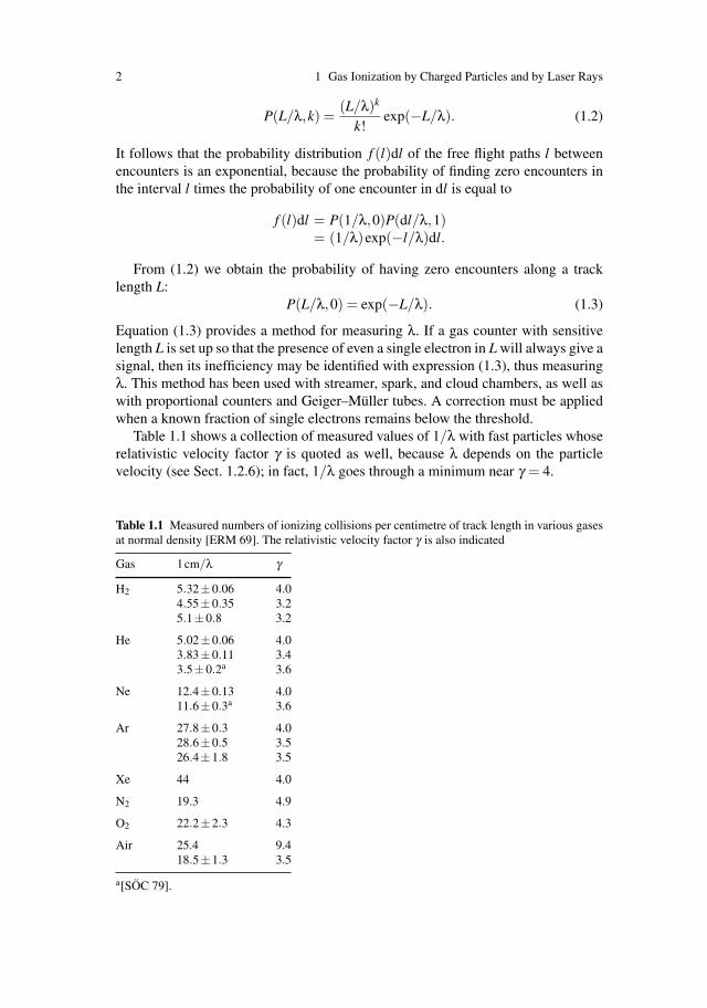
Table 1.1 shows a collection of measured values of 1/λ with fast particles whoserelativistic velocity factor γ is quoted as well, because λ depends on the particlevelocity (see Sect. 1.2.6); in fact, 1/λ goes through a minimum near γ = 4.
Table 1.1 Measured numbers of ionizing collisions per centimetre of track length in various gasesat normal density [ERM 69]. The relativistic velocity factor γ is also indicated
Gas 1cm/λ γ
H2 5.32±0.06 4.04.55±0.35 3.25.1±0.8 3.2
He 5.02±0.06 4.03.83±0.11 3.43.5±0.2a 3.6
Ne 12.4±0.13 4.011.6±0.3a 3.6
Ar 27.8±0.3 4.028.6±0.5 3.526.4±1.8 3.5
Xe 44 4.0
N2 19.3 4.9
O2 22.2±2.3 4.3
Air 25.4 9.418.5±1.3 3.5
a[SOC 79].

1.1 Gas Ionization by Fast Charged Particles 3
Table 1.2 Minimal primary ionization cross-sections σp for charged particles in some gases, andrelativistic velocity factor γmin of the minimum, according to measurements done by Rieke andPrepejchal [RIE 72]
Gas σp(10−20 cm2) γmin Gas σp(10−20 cm2) γmin
H2 18.7 3.81 i-C4H10 333 3.56He 18.6 3.68 n-C5H12 434 3.56Ne 43.3 3.39 neo-C5H12 433 3.45Ar 90.3 3.39 n-C6H14 526 3.51Xe 172 3.39 C2H2 126 3.60O2 92.1 3.43 C2H4 161 3.58CO2 132 3.51 CH3OH 155 3.65C2H6 161 3.58 C2H5OH 230 3.51C3H8 269 3.47 (CH3)2CO 277 3.54
In Table 1.2 we present additional measurements of a larger number of gasesthat are employed in drift chambers. These primary ionization cross-sections σp
were measured by Rieke and Prepejchal [RIE 72] in the vicinity of the minimumat different values of γ and interpolated to the minimum γmin
p at γmin, using theparametrization of the Bethe–Bloch formula (see Sect. 1.2.7). The mean free path λis related to σp by the number density Nm of molecules:
λ = 1/(Nmσp).
The measurement errors are within ±4% (see the original paper for details). Incomparison with the values presented in Table 1.1, the measurements are in roughagreement, except for argon.
1.1.2 Different Ionization Mechanisms
We distinguish between primary and secondary ionization. In primary ionization,one or sometimes two or three electrons are ejected from the atom A encounteredby the fast particle, say a π meson:
πA → πA+e−, πA++e−e−, . . . (1.4)
Most of the charge along a track is from secondary ionization where the electronsare ejected from atoms not encountered by the fast particle. This happens either incollisions of ionization electrons with atoms,
e−A → e−A+e−, e−A++e−e−, (1.5)
or through intermediate excited states A∗. An example is the following chain ofreactions involving the collision of the excited state with a second species, B, ofatoms or molecules that is present in the gas:
πA → πA∗ (1.6a)

4 1 Gas Ionization by Charged Particles and by Laser Rays
ore−A → e−A∗, (1.6b)
A∗B → AB+e−. (1.7)
Reaction (1.7) occurs if the excitation energy of A∗ is above the ionization potentialof B. In drift chambers, A∗ is often the metastable state of a noble gas created inreaction (1.6b), and B is one of the molecular additives (quenchers) that are requiredfor the stability of proportional wire operation; A∗ may also be an optical excitationwith a long lifetime due to resonance trapping. These effects are known under thenames of Penning effect (involving metastables) and Jesse effect (involving opticalexcitations, also used more generally); obviously they depend very strongly on thegas composition and density.
Another example of secondary ionization through intermediate excitation hasbeen observed in pure rare gases where an excited molecule A∗
2 has a stable ionizedground state A+
2 :A∗A → A∗
2 → A+2 e−. (1.8)
The different contributions of processes (1.5–1.8) are in most cases unknown. Forfurther references, we recommend the proceedings of the conferences dedicated tothese phenomena, for example the Symposium on the Jesse Effect and Related Phe-nomena [PRO 74].
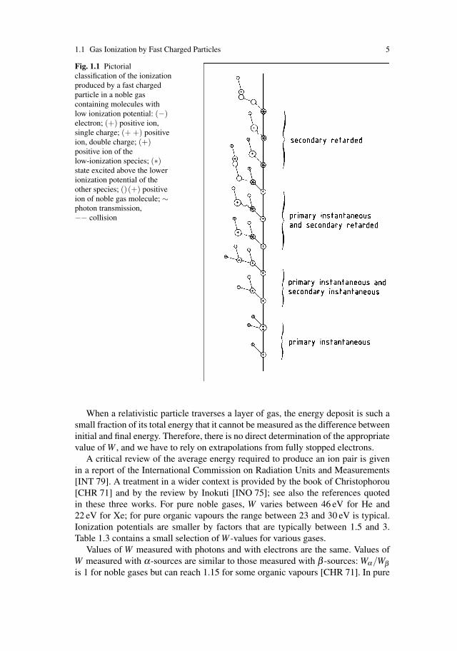
A pictorial summary of the processes discussed is given in Fig. 1.1.
1.1.3 Average Energy Required to Produce One Ion Pair
Only a certain fraction of all the energy lost by the fast particle is spent in ionization.The total amount of ionization from all processes is characterized by the energy Wthat is spent, on the average, on the creation of one free electron. We write
W 〈NI〉 = L
⟨dEdx
⟩, (1.9)
where 〈NI〉 is the average number of ionization electrons created along a trajectoryof length L, and 〈dE/dx〉 is the average total energy loss per unit path length of thefast particle; W must be measured for every gas mixture.
Many measurements of W have been performed since the advent of radioactiv-ity, using radioactive and artificial sources of radiation. The amount of ionizationproduced by particles that lose all their energy in the gas is measured by ionizationchambers or proportional counters. The value of W in this case is the ratio of theinitial energy to the number of ion pairs. The energy W depends on the gas – itscomposition and density – and on the nature of the particle. Experimentally it isfound that W is independent of the initial energy above a few keV for electrons anda few MeV for alpha-particles, which is a remarkable fact.
1.1 Gas Ionization by Fast Charged Particles 5
Fig. 1.1 Pictorialclassification of the ionizationproduced by a fast chargedparticle in a noble gascontaining molecules withlow ionization potential: (−)electron; (+) positive ion,single charge; (+ +) positiveion, double charge; (+)positive ion of thelow-ionization species; (∗)state excited above the lowerionization potential of theother species; ()(+) positiveion of noble gas molecule; ∼photon transmission,−− collision
When a relativistic particle traverses a layer of gas, the energy deposit is such asmall fraction of its total energy that it cannot be measured as the difference betweeninitial and final energy. Therefore, there is no direct determination of the appropriatevalue of W , and we have to rely on extrapolations from fully stopped electrons.
A critical review of the average energy required to produce an ion pair is givenin a report of the International Commission on Radiation Units and Measurements[INT 79]. A treatment in a wider context is provided by the book of Christophorou[CHR 71] and by the review by Inokuti [INO 75]; see also the references quotedin these three works. For pure noble gases, W varies between 46 eV for He and22 eV for Xe; for pure organic vapours the range between 23 and 30 eV is typical.Ionization potentials are smaller by factors that are typically between 1.5 and 3.Table 1.3 contains a small selection of W -values for various gases.
Values of W measured with photons and with electrons are the same. Values ofW measured with α-sources are similar to those measured with β -sources: Wα/Wβis 1 for noble gases but can reach 1.15 for some organic vapours [CHR 71]. In pure
6 1 Gas Ionization by Charged Particles and by Laser Rays
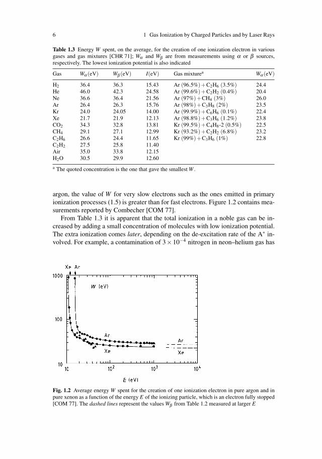
Table 1.3 Energy W spent, on the average, for the creation of one ionization electron in variousgases and gas mixtures [CHR 71]; Wα and Wβ are from measurements using α or β sources,respectively. The lowest ionization potential is also indicated
Gas Wα (eV) Wβ (eV) I(eV) Gas mixturea Wα (eV)
H2 36.4 36.3 15.43 Ar (96.5%)+C2H6 (3.5%) 24.4He 46.0 42.3 24.58 Ar (99.6%)+C2H2 (0.4%) 20.4Ne 36.6 36.4 21.56 Ar (97%)+CH4 (3%) 26.0Ar 26.4 26.3 15.76 Ar (98%)+C3H8 (2%) 23.5Kr 24.0 24.05 14.00 Ar (99.9%)+C6H6 (0.1%) 22.4Xe 21.7 21.9 12.13 Ar (98.8%)+C3H6 (1.2%) 23.8CO2 34.3 32.8 13.81 Kr (99.5%)+C4H8-2 (0.5%) 22.5CH4 29.1 27.1 12.99 Kr (93.2%)+C2H2 (6.8%) 23.2C2H6 26.6 24.4 11.65 Kr (99%)+C3H6 (1%) 22.8C2H2 27.5 25.8 11.40Air 35.0 33.8 12.15H2O 30.5 29.9 12.60
a The quoted concentration is the one that gave the smallest W .
argon, the value of W for very slow electrons such as the ones emitted in primaryionization processes (1.5) is greater than for fast electrons. Figure 1.2 contains mea-surements reported by Combecher [COM 77].
From Table 1.3 it is apparent that the total ionization in a noble gas can be in-creased by adding a small concentration of molecules with low ionization potential.The extra ionization comes later, depending on the de-excitation rate of the A∗ in-volved. For example, a contamination of 3×10⁻⁴ nitrogen in neon–helium gas has
Fig. 1.2 Average energy W spent for the creation of one ionization electron in pure argon and inpure xenon as a function of the energy E of the ionizing particle, which is an electron fully stopped[COM 77]. The dashed lines represent the values Wβ from Table 1.2 measured at larger E

1.1 Gas Ionization by Fast Charged Particles 7
caused secondary retarded ionization that amounted to 60% of the primary, withmean retardation times around 1μs [BLU 74].
Whether the number of primary encounters that lead to ionization can be in-creased in the same manner is not so clear; the fast particle would have to excite thestate A∗ in a primary collision (reaction (1.6a)). A metastable state does not have adipole transition to the ground state and is therefore not easily excited by the fastparticle.
1.1.4 The Range of Primary Electrons
Primary electrons are emitted almost perpendicular to the track as their momentumremains very small compared to the one of the track. They lose their kinetic energyE in collisions with the gas molecules, scattering almost randomly and producingsecondary electrons, until they have lost their kinetic energy. A practical range R canbe defined as the thickness of the layer of material they cross before being stopped.The empirical relation
R(E) = AE
(1− B
1+CE
)(1.10)
with A = 5.37×10⁻⁴ g cm−2 keV−1, B = 0.9815, and C = 3.1230×10⁻³ keV−1 isshown in Fig. 1.3 and compared with experimental data in the range between 300 eVand 20 MeV. It is shown in [KOB 68] that the parametrization (1.10) is applicableto all materials with low and intermediate atomic number Z. In the absence of low-energy data this curve may be taken as a basis for an extrapolation to lower E. Below1 keV the relation reads
R(E) = 9.93( μg
cm2 keV
)E.
In argon N.T.P. an electron of 1 keV is stopped in about 30μm, and one of 10 keVin about 1.5 mm. Only 0.05% of the collisions between the particle and the gasmolecules produce primary electrons with kinetic energy larger than 10 keV. Wewill compute these probabilities in Sect. 1.2.4.
1.1.5 The Differential Cross-section dσ/dE
Every act of ionization is a quantum mechanical transition initiated by the fieldof the fast particle and the field created indirectly by the neighbouring polarizableatoms. A complete calculation would involve the transition amplitudes of all theatomic states and does not exist.
For the detection of particles, what we have to know in the first place is theamount of ionization along the track and the associated fluctuation phenomena. For

8 1 Gas Ionization by Charged Particles and by Laser Rays
Fig. 1.3 Practical range versus kinetic energy for electrons in aluminium. The data points arefrom various authors, which can be traced back consulting [KOB 68]. The curve is aparametrization according to (1.10)
this it is sufficient to determine for an act of primary ionization with what probabil-ities it will result in a total ionization of 1,2, . . ., or n electrons. The total ionizationover a piece of track and its frequency distribution can then be determined by sum-ming over all the primary encounters in that piece.
Using the concept of the average energy W required to produce one ion pair –be it a constant as in (1.9) or a function of the energy of the primary electron asin Fig. 1.2 – the problem is reduced to finding the energy spectrum F(E)dE ofthe primary electrons, or, equivalently, the corresponding differential cross-sectiondσ/dE. Once this is known, we obtain λ and F(E) with the relations
1/λ =∫
NdσdE
dE
and
F(E) =N(dσ/dE)
1/λ,
where N is the electron number density in the gas and dσ/dE the differential cross-section per electron to produce a primary electron with an energy between E andE +dE.

1.2 Calculation of Energy Loss 9
1.2 Calculation of Energy Loss
In order to calculate dσ/dE we will begin by investigating the average total en-ergy loss per unit distance, 〈dE/dx〉, of a moving charged particle in a polarizablemedium. Here a classical calculation is appropriate in which the medium is treatedas a continuum characterized by a complex dielectric constant ε = ε1 + iε2. Later onwe will interpret the resulting integral over the lost energy in a quantum mechani-cal sense.
1.2.1 Force on a Charge Travelling Through a Polarizable Medium
It is the field Elong opposite to its direction of motion, created by the moving particlein the medium at its own space point, which produces the force equal to the energyloss per unit distance
〈dE/dx〉 = eElong,
where e is the charge of the moving particle. We follow the method of Landau andLifshitz [LAN 60] in the form used by Allison and Cobb [ALL 80].
Maxwell’s equations in an isotropic, homogeneous, non-magnetic medium are
∇·H = 0,
∇×E = −1c
∂H
∂ t,
∇· (εE) = 4π–,
∇×H =1c
∂ (εE)∂ t
+4πc
j.
(1.11)
Since there will be no confusion between the electric field vector E and the energylost, E, we will use the customary symbols.
The charge density and the flux are given by the particle moving with velocity βc:
– = eδ 3(r−βct), j = βc–. (1.12)
We work in the Coulomb gauge and introduce the potentials φ and A:
H = ∇×A,
∇·A = 0,
E = −1c
∂A
∂ t−∇φ .
(1.13)
Equations (1.11), expressed in terms of the potentials, are
∇· (ε∇φ) = −4πeδ 3(r−βct),
−∇2A = − 1c2
∂∂ t
(ε
∂A
∂ t
)1c
∂∂ t
(ε∇φ)+4πeβδ 3(r−βct).(1.14)
10 1 Gas Ionization by Charged Particles and by Laser Rays
The solutions can be found in terms of the Fourier transforms φ(k,ω) and A(k,ω)of the potentials.
The Fourier transform F(k,ω) of a vector field F(r, t) is given by
F(k,ω) =1
(2π)2
∫d3r dt F(r, t)exp(ik ·r− iωt),
F(r, t) =1
(2π)2
∫d3k dω F(k,ω)exp(ik ·r− iωt).
(1.15)
The solutions of (1.14) are
φ(k,ω) = 2eδ (ω −k ·βc)/k2ε,
A(k,ω) = 2eωk/k2c−β
(−k2 + εω2/c2)δ (ω −k ·βc).
(1.16)
Using the third of (1.13), the electric field for every point is calculated according to
E(r, t) =1
(2π)2
∫iωc{A(k,ω)− ikφ(k,ω)exp[i(k ·r−ωt)]}d3k dω, (1.17)
and the energy loss per unit length is
〈dE/dx〉 = eE(βct, t) ·β/β , (1.18)
which is independent of t because the field created in the medium is travelling withthe particle. This may be seen by inserting (1.16) into (1.17).
In the evaluation of (1.17) with the help of (1.16) we integrate over the twodirections of k using the fact that the isotropic medium has a scalar ε . We furtheruse ε(−ω) = ε∗(ω) and obtain finally
⟨dEdx
⟩=
2e2
β 2π
∞∫0
dω∞∫
ω/βc
dk
[ωk
(β 2 − ω2
k2c2
)
×Im1
−k2c2 + εω2 − ωkc2 Im
(1ε
)]. (1.19)
The lower limit of the integral over k depends on the particle velocity βc and isexplained later.
The energy loss is determined by the manner in which the complex dielectricconstant ε depends on the wave number k and the frequency ω . Once ε(k,ω) isspecified, 〈dE/dx〉 can be calculated for every β ;ε(k,ω) is, in principle, givenby the structure of the atoms of the medium. In practice, a simplifying model issufficient.
1.2 Calculation of Energy Loss 11
1.2.2 The Photo-Absorption Ionization Model
Allison and Cobb [ALL 80] have made a model of ε(k,ω) based on the measuredphoto-absorption cross-section σγ(ω). A plane light-wave travelling along x is at-tenuated in the medium if the imaginary part of the dielectric constant is larger thanzero. The wave number k is related to the frequency ω by
k =√
εω/c (ε = ε1 + iε2). (1.20)
It causes a damping factor e−αx/2 in the propagation function and e−αx in the inten-sity with
α = 2(ω/c)Im√
ε ≈ (ω/c)ε2. (1.21)
The second equality holds if ε1 −1, ε2 1 such as for gases.In terms of free photons traversing a medium that has electron density N and
atomic charge Z, the attenuation is given by the photo-absorption cross-sectionσγ(ω):
σγ(ω) =ZN
α ≈ ZN
ωc
ε2(ω). (1.22)
The cross-section σγ(ω), and therefore ε2(ω), is known, for many gases, from mea-surements using synchrotron radiation. The real part of ε is then derived from thedispersion relation
ε1(ω)−1 =2π
P
∞∫0
xε2(x)x2 −ω2 dx (1.23)
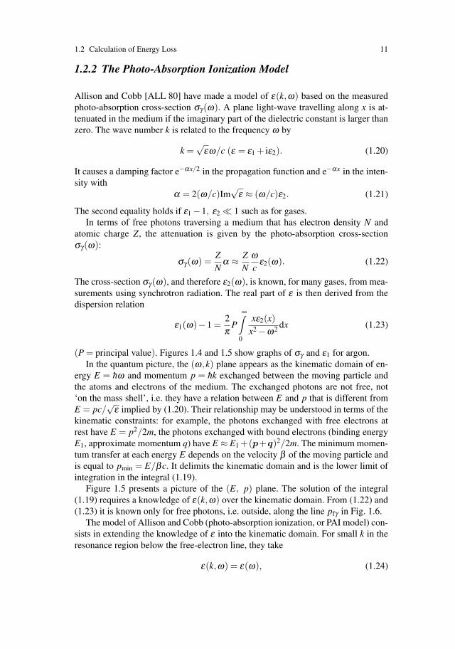
(P = principal value). Figures 1.4 and 1.5 show graphs of σγ and ε1 for argon.In the quantum picture, the (ω,k) plane appears as the kinematic domain of en-
ergy E = hω and momentum p = hk exchanged between the moving particle andthe atoms and electrons of the medium. The exchanged photons are not free, not‘on the mass shell’, i.e. they have a relation between E and p that is different fromE = pc/
√ε implied by (1.20). Their relationship may be understood in terms of the
kinematic constraints: for example, the photons exchanged with free electrons atrest have E = p2/2m, the photons exchanged with bound electrons (binding energyE1, approximate momentum q) have E ≈ E1 +(p+q)2/2m. The minimum momen-tum transfer at each energy E depends on the velocity β of the moving particle andis equal to pmin = E/βc. It delimits the kinematic domain and is the lower limit ofintegration in the integral (1.19).
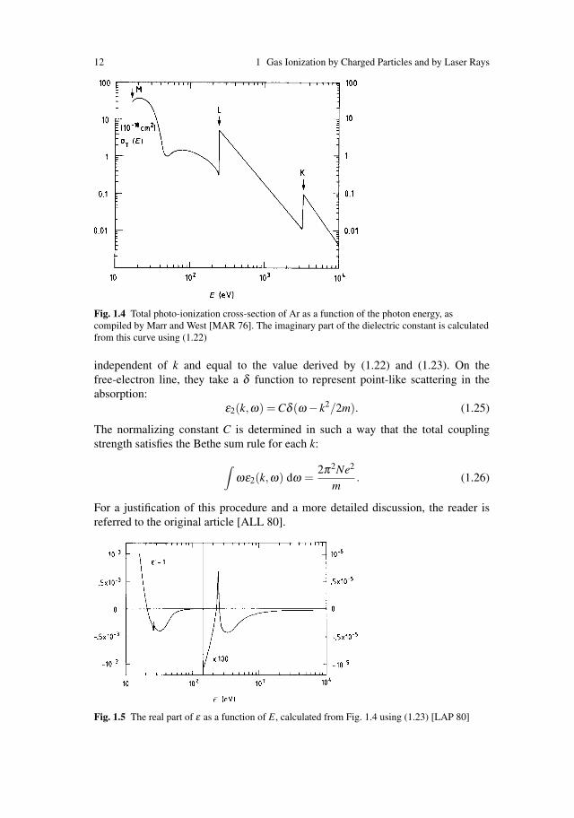
Figure 1.5 presents a picture of the (E, p) plane. The solution of the integral(1.19) requires a knowledge of ε(k,ω) over the kinematic domain. From (1.22) and(1.23) it is known only for free photons, i.e. outside, along the line pfγ in Fig. 1.6.
The model of Allison and Cobb (photo-absorption ionization, or PAI model) con-sists in extending the knowledge of ε into the kinematic domain. For small k in theresonance region below the free-electron line, they take
ε(k,ω) = ε(ω), (1.24)
12 1 Gas Ionization by Charged Particles and by Laser Rays
Fig. 1.4 Total photo-ionization cross-section of Ar as a function of the photon energy, ascompiled by Marr and West [MAR 76]. The imaginary part of the dielectric constant is calculatedfrom this curve using (1.22)
independent of k and equal to the value derived by (1.22) and (1.23). On thefree-electron line, they take a δ function to represent point-like scattering in theabsorption:
ε2(k,ω) = Cδ (ω − k2/2m). (1.25)
The normalizing constant C is determined in such a way that the total couplingstrength satisfies the Bethe sum rule for each k:
∫ωε2(k,ω) dω =
2π2Ne2
m. (1.26)
For a justification of this procedure and a more detailed discussion, the reader isreferred to the original article [ALL 80].
Fig. 1.5 The real part of ε as a function of E, calculated from Fig. 1.4 using (1.23) [LAP 80]

1.2 Calculation of Energy Loss 13
Fig. 1.6 Kinematic domain of(ω,k) or (E, p) of the electro-magnetic radiation exchangedbetween the fast particle (β )and the medium. The mini-mum momentum exchangedis p = E/βc; the momentumexchanged to a free electronis pfe =
√2mE/c2. The mo-
menta exchanged with boundelectrons are smeared outaround the free-electron line;pmin delimits the physicaldomain, pfγ is the free pho-ton line
Using (1.22–1.25), we are now able to integrate expression (1.19) for 〈dE/dx〉over k. What remains is an integral over ω:
⟨dEdx
⟩=
∞∫0
dωe2
β 2c2π
[NcZ
σγ(ω) ln2mc2β 2
hω[(1−β 2ε1)2 +β 4ε22 ]1/2
+ω(
β 2 − ε1
|ε|2)
θ +1
Zω
ω∫0
σγ(ω ′)dω ′]. (1.27)
Here we have obtained the energy loss per unit path length in the framework of theelectrodynamics of a continuous medium, although our knowledge of ε(k,ω) wasactually inspired by a picture of photon absorption and collision.
At this point we leave the frame given by the classical theory and recognize theenergy loss as being caused by a number of discrete collisions per unit length, eachwith an energy transfer E = hω . Therefore, we reinterpret the integrand of (1.27)to mean E times a probability of energy transfer per unit path per unit interval ofE. Now a collision probability per unit path is a cross-section times the density N.Therefore, we write the integral (1.27) in the form
⟨dEdx
⟩=
∞∫0
ENdσdE
h dω. (1.28)
This gives us the differential energy transfer cross-section per electron:
dσdE
=α
β 2πσγ(E)
EZln
2mc2β 2
E[(1−β 2ε1)2 +β 4ε22 ]1/2
+α
β 2π
⎡⎣ Z
Nhc
(β 2 − ε1
|ε|2)
θ +1
ZE2
E∫0
σγ(E ′)dE ′
⎤⎦ . (1.29)

14 1 Gas Ionization by Charged Particles and by Laser Rays
The spectrum of energy transfer is determined by expression (1.29). The normalizeddifferential probability per unit energy is
F(E) =N(dσ/dE)∫N(dσ/dE)dE
, (1.30)
where N is the number of electrons per unit volume; ε = ε1 + iε1 is to be obtainedusing (1.22) and (1.23); θ = arg(1 − ε1β 2 + iε2β 2); and α is the fine-structureconstant.
The number of primary encounters per unit length is given by
1/λ =∫
NdσdE
dE. (1.31)
In the gas of a drift chamber the largest possible energy transfers cause secondaryelectron tracks which do not belong to the primary track. Depending on the exactmethod of observation, there is always an effective cut-off Emax for the observableenergy transfer, which is independent of β . For simplicity, we keep the ‘∞’ as theupper limit of integration. Figure 1.7 shows the energy spectrum for argon accord-ing to a numerical calculation along this line by Lapique and Piuz [LAP 80]; theyhave evaluated the model of Chechin et al. [CHE 72, ERM 77], which is very sim-ilar to the PAI model. The second peak beyond E = 240eV, which is due to thecontribution of the L shell, is easily visible.
Fig. 1.7 Distribution of energy transfer calculated by Lapique and Piuz for argon at γ = 1000,based on the formula by Chechin et al. [CHE 76], similar to our (1.29). Adapted from Table 1.1 of[LAP 80]

1.2 Calculation of Energy Loss 15
1.2.3 Behaviour for Large E
For energies above the highest atomic binding energy EK, the fast particle undergoeselastic scattering on the atomic electrons as if they were free, and (1.29) becomesthe differential cross-section for Rutherford scattering on one electron. Using (1.26)and (1.27) we find
dσdE
→ 2πr2e
β 2
mc2
E2 (E � EK), (1.32)
where re is the classical electron radius, equal to e2/mc2 = 2.82× 10⁻¹³ cm. Thishappens because the third term in (1.29) is the only one surviving at large E, whereσγ(E) vanishes quickly so that the sum rule (1.26) applies, together with (1.22).
This behaviour at large E means that the energy spectrum F(E) has an extremelylong tail. Although
∫F(E)dE converges, the mean transferred energy per collision,
〈E〉, has a logarithmic divergence,
〈E〉 =∫
EF(E)dE =∫
dE/E ∝ logE. (1.33)
This requires a careful interpretation of the mean energy transfer, as shown in thefollowing sections. There is no danger that the mean transferred energy 〈E〉 divergesin the practical application because there is always an upper cut-off for E at work inthe integral (1.33), which depends on the situation. This is discussed in Sec. 1.2.8.
1.2.4 Cluster-Size Distribution
An effective description of the ionization left by the particle along its trajectory isprovided by a probability distribution of the number of electrons liberated directlyor indirectly with each primary encounter. It is known under the name cluster-sizedistribution, because the secondary electrons are usually created in the immediatevicinity of the primary encounter and, together with the primary electrons, formclusters of one or several – sometimes many – electrons. Although the secondaryelectrons are not always so well localized, we will use this name.
In order to calculate the cluster-size distribution P(k) we need to know the spec-trum of energy loss, F(E)dE, and, for each E, the probability p(E, k) of producingexactly k ionization electrons. The cluster-size distribution is obtained by integrationover the energy:
P(k) =∫
F(E)p(E,k)dE. (1.34)
We may also form the integrated probability Q( j) that a cluster has more than jelectrons:
Q( j) = 1−j
∑k=1
P(k). (1.35)
16 1 Gas Ionization by Charged Particles and by Laser Rays
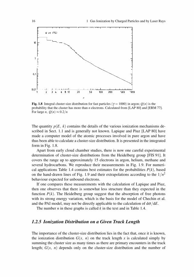
Fig. 1.8 Integral cluster-size distribution for fast particles (γ = 1000) in argon; Q(n) is theprobability that the cluster has more than n electrons. Calculated from [LAP 80] and [ERM 77].For large n, Q(n) ≈ 0.2/n
The quantity p(E, k) contains the details of the various ionization mechanisms de-scribed in Sect. 1.1 and is generally not known. Lapique and Piuz [LAP 80] havemade a computer model of the atomic processes involved in pure argon and havethus been able to calculate a cluster-size distribution. It is presented in the integratedform in Fig. 1.8.
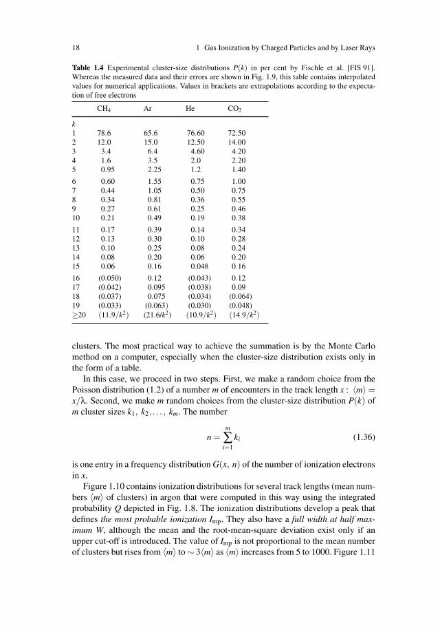
Apart from early cloud chamber studies, there is now one careful experimentaldetermination of cluster-size distributions from the Heidelberg group [FIS 91]. Itcovers the range up to approximately 15 electrons in argon, helium, methane andseveral hydrocarbons. We reproduce their measurements in Fig. 1.9. For numeri-cal applications Table 1.4 contains best estimates for the probabilities P(k), basedon the hand-drawn lines of Fig. 1.9 and their extrapolations according to the 1/n2
behaviour expected for unbound electrons.If one compares these measurements with the calculation of Lapique and Piuz,
then one observes that there is somewhat less structure than they expected in thefunction P(k). The Heidelberg group suggest that the absorption of free photonswith its strong energy variation, which is the basis for the model of Chechin et al.and the PAI model, may not be directly applicable to the calculation of dσ/dE.
The number n in these graphs is called k in the text and in Table 1.4.
1.2.5 Ionization Distribution on a Given Track Length
The importance of the cluster-size distribution lies in the fact that, once it is known,the ionization distribution G(x, n) on the track length x is calculated simply bysumming the cluster size as many times as there are primary encounters in the tracklength; G(x, n) depends only on the cluster-size distribution and the number of

1.2 Calculation of Energy Loss 17
Fig. 1.9 Experimental cluster-size distributions from [FIS 91]. The continuous lines arehand-drawn interpolations whereas the broken lines are extrapolations corresponding to the1/n2-law expected for large n
18 1 Gas Ionization by Charged Particles and by Laser Rays
Table 1.4 Experimental cluster-size distributions P(k) in per cent by Fischle et al. [FIS 91].Whereas the measured data and their errors are shown in Fig. 1.9, this table contains interpolatedvalues for numerical applications. Values in brackets are extrapolations according to the expecta-tion of free electrons
CH4 Ar He CO2
k1 78.6 65.6 76.60 72.502 12.0 15.0 12.50 14.003 3.4 6.4 4.60 4.204 1.6 3.5 2.0 2.205 0.95 2.25 1.2 1.40
6 0.60 1.55 0.75 1.007 0.44 1.05 0.50 0.758 0.34 0.81 0.36 0.559 0.27 0.61 0.25 0.4610 0.21 0.49 0.19 0.38
11 0.17 0.39 0.14 0.3412 0.13 0.30 0.10 0.2813 0.10 0.25 0.08 0.2414 0.08 0.20 0.06 0.2015 0.06 0.16 0.048 0.16
16 (0.050) 0.12 (0.043) 0.1217 (0.042) 0.095 (0.038) 0.0918 (0.037) 0.075 (0.034) (0.064)19 (0.033) (0.063) (0.030) (0.048)≥20 (11.9/k2) (21.6/k2) (10.9/k2) (14.9/k2)
clusters. The most practical way to achieve the summation is by the Monte Carlomethod on a computer, especially when the cluster-size distribution exists only inthe form of a table.
In this case, we proceed in two steps. First, we make a random choice from thePoisson distribution (1.2) of a number m of encounters in the track length x : 〈m〉 =x/λ. Second, we make m random choices from the cluster-size distribution P(k) ofm cluster sizes k1, k2, . . . , km. The number
n =m
∑i=1
ki (1.36)
is one entry in a frequency distribution G(x, n) of the number of ionization electronsin x.
Figure 1.10 contains ionization distributions for several track lengths (mean num-bers 〈m〉 of clusters) in argon that were computed in this way using the integratedprobability Q depicted in Fig. 1.8. The ionization distributions develop a peak thatdefines the most probable ionization Imp. They also have a full width at half max-imum W, although the mean and the root-mean-square deviation exist only if anupper cut-off is introduced. The value of Imp is not proportional to the mean numberof clusters but rises from 〈m〉 to ∼ 3〈m〉 as 〈m〉 increases from 5 to 1000. Figure 1.11

1.2 Calculation of Energy Loss 19
Fig. 1.10 Ionization distri-bution obtained by summingm times the cluster-size dis-tribution of Fig. 1.8, usingthe method described inSect. 1.2.3. On 1 cm of Arin normal conditions thereare, on the average, 〈m〉 = 35clusters (γ = 1000); the eightdistributions then correspondto track lengths of 0.14,0.29, 0.57, 1.4, 2.9, 5.7, 14,and 29 cm

20 1 Gas Ionization by Charged Particles and by Laser Rays
Fig. 1.11 Values of the mostprobable number of electrons(expressed in units of 〈m〉)as a function of the meannumber 〈m〉 of clusters inAr, obtained from the data ofFig. 1.8
shows this increase. It does not obey a simple law because it is influenced by theatomic structure of argon. Neglecting the atomic structure, it approaches a straightline; compare the remarks made on Δmp after (1.49). The distributions of Fig. 1.10also become more peaked, so that the ratio W/Imp decreases from ∼ 1.3 to ∼ 0.3 inthis range of 〈m〉.
Relative widths W/Imp of measured pulse-height distributions quoted by Walenta[WAL 81] are shown in Fig. 1.11 as a function of the gas sample thickness pL. Theratio decreases with increasing pL. If we parametrize the decrease in the form of apower law, (
WImp
)1
:
(WImp
)2
= [(pL)1 : (pL)2]k, (1.37)
then from Fig. 1.12 we get k between −0.2 and −0.4. Since the ionization distri-bution depends only on the cluster-size distribution and the number of clusters, itdepends on the sample length L and the gas pressure p through the product pL.
Fig. 1.12 Measured rela-tive widths of pulse-heightdistributions as collected byWalenta [WAL 81]. The plotshows ten different experi-ments with the gas samplethickness pL varying between0.6 and 15 cm bar. The line isdrawn to guide the eye
1.2 Calculation of Energy Loss 21
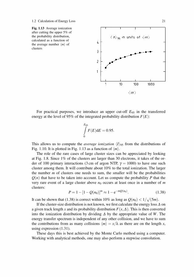
Fig. 1.13 Average ionizationafter cutting the upper 5% ofthe probability distribution,calculated as a function ofthe average number 〈m〉 ofclusters
For practical purposes, we introduce an upper cut-off E95 in the transferredenergy at the level of 95% of the integrated probability distribution F(E):
E95∫0
F(E)dE = 0.95.
This allows us to compute the average ionization 〈I〉95 from the distributions ofFig. 1.10. It is plotted in Fig. 1.13 as a function of 〈m〉.
The role of the rare cases of large cluster sizes can be appreciated by lookingat Fig. 1.8. Since 1% of the clusters are larger than 30 electrons, it takes of the or-der of 100 primary interactions (3 cm of argon NTP, γ = 1000) to have one suchcluster among them. It will contribute about 10% to the total ionization. The largerthe number m of clusters one needs to sum, the smaller will be the probabilitiesQ(n) that have to be taken into account. Let us compute the probability P that thevery rare event of a large cluster above n0 occurs at least once in a number of mclusters:
P = 1− [1−Q(n0)]m ≈ 1− e−mQ(n0). (1.38)
It can be shown that (1.38) is correct within 10% as long as Q(n0) < 1/√
(5m).If the cluster-size distribution is not known, we first calculate the energy loss Δ on
a given track length x and its probability distribution F(x,Δ). This is then convertedinto the ionization distribution by dividing Δ by the appropriate value of W . Theenergy transfer spectrum is independent of any other collision, and we have to sumthe contributions from as many collisions 〈m〉 = x/λ as there are on the length x,using expression (1.31).
These days this is best achieved by the Monte Carlo method using a computer.Working with analytical methods, one may also perform a stepwise convolution.

22 1 Gas Ionization by Charged Particles and by Laser Rays
For example,
F(2λ,Δ) =∞∫
0
F(Δ −E)F(E)dE,
F(4λ,Δ) =∞∫
0
F(2λ,Δ −E)F(2λ,E) dE, etc. (1.39)
The review of Bichsel and Saxon [BIC 75] contains more details about how to buildup F(x,Δ).
Another way of constructing F(x,Δ) from F(E) was invented by Landau in 1944[LAN 44]. He expressed the change of F(x,Δ) along a length dx by the differencein the number of particles which, because of ionization losses along dx, acquire agiven energy E and the number of particles which leave the given energy intervalnear Δ :
∂∂x
F(x,Δ) =∞∫
0
F(E)[F(x,Δ −E)−F(x,Δ)] dE. (1.40)
(For the upper limit of integration, one may write ∞ because F(x,Δ) = 0 for Δ < 0.)The solution of (1.40) is found with the help of the Laplace transform F(x, p), whichis related to the energy loss distribution by
F(x, p) =∞∫
0
F(x,Δ)e−pΔ dΔ , (1.41)
F(x,Δ) =1
2πi
+i∞+σ∫−i∞+σ
epΔ F(x, p) dp. (1.42)
Here the integration is to the right (σ > 0) of the imaginary axis of p. Multiplyingboth sides of (1.40) by a e−pΔ and integrating over Δ , we get
∂∂x
F(x, p) = −F(x, p)∞∫
0
F(E)(1− e−pE) dE, (1.43)
which integrates to
F(x, p) = exp
⎡⎣−x
∞∫0
F(E)(1− e−pE) dE
⎤⎦ , (1.44)
because the boundary condition is F(0,Δ) = δ (Δ) or F(0, p) = 1. Inserting (1.41)into (1.44), Landau obtained the general expression for the energy loss distribution,valid for any F(E):
F(x,Δ) =1
2πi
+i∞+σ∫−i∞+σ
exp
⎡⎣pΔ − x
∞∫0
F(E)(1− e−pE) dE
⎤⎦ dp. (1.45)

1.2 Calculation of Energy Loss 23
This relation was evaluated by Landau for a simplified form of F(E) that is ap-plicable at energies far above the atomic binding energies where the scatteringcross-section is determined by Rutherford scattering and where the atomic struc-ture can be ignored (see (1.32)). Inserting
F(E) =2πr2
e
β 2
mc2
E2 N (1.46)
into (1.45), Landau was able to show that the probability distribution was given bya universal function φ(λ):
F(x,Δ) dΔ = φ(
Δ −Δmp
ξ
)d
(Δ −Δmp
ξ
). (1.47)
Here Δmp is the most probable energy loss, and ξ is a scaling factor for the energyloss, proportional to x:
ξ = x2πr2e
mc2
β 2 N. (1.48)
The function φ(λ) and its integral ψ(λ) are given as a graph in Fig. 1.14. Computerprograms exist for the calculation of φ and for the random generation of Landau-distributed numbers: see Kolbig and Schorr [KOL 84]. The integral probability foran energy loss exceeding Δ is
∞∫Δ
F(x,Δ ′) dΔ ′ = ψ(
Δ −Δmp
ξ
). (1.49)
We notice that 10% of the cases lie above the value of Δ that is three times theFWHM above the most probable value. For large positive values of the argument,φ(λ) tends to 1/λ2, ψ(λ) tends to 1/λ. The assumption (1.47) makes the Landau
Fig. 1.14 Landau’s functionφ(λ) and its integral ψ(λ).The scale on the left refers toφ , the one on the right to ψ

24 1 Gas Ionization by Charged Particles and by Laser Rays
curve a valid description of the energy loss fluctuations only in a regime of largeΔ (corresponding to x ≈ 170cm in normal argon gas, according to an analysis of[CHE 76] [see also Fig. 1.21]). We skip a discussion of Landau’s expression for Δmp
and of the normalization of his F(E). Let us remark, however, that, as a function ofthe length x, Δmp is proportional to x logx. In practice, the Landau curve is oftenused to parametrize energy loss distributions with a two-parameter fit of ξ and Δmp,without reference to the theoretical expressions for them.
Generalizations of the Landau theory have been given by Blunck and Leisegang[BLU 50], Vavilov [VAV 57], and others. The interested reader is referred to themonograph by Bugadov, Merson, Sitar and Chechin [BUG 88] for a comparison ofthese theories of energy loss.
When the summation of the energy lost over the length x has been achieved withany of the methods mentioned above, the energy loss distribution must be convertedinto an ionization distribution. We have to make the assumption that to every energyloss Δ there corresponds, on the average, a number n of ion pairs according to therelation
Δ = nW, (1.50)
where W is the average energy for producing an ion pair (Sect. 1.1.3). Expression(1.50) is to hold independently of the size or the composition of Δ (whether thereare one large or many small transfers), and W is to be the constant measured withfully stopped electrons. It is hard to ascertain the error that we introduce with thisassumption. The W measured with fully stopped electrons is known to increase forenergy transfers below ∼ 1keV (Fig. 1.2).
Using (1.50), we obtain the probability distribution G(x, n) of the number n ofionization electrons produced on the track length x:
G(x,n) = F(x,nW )W. (1.51)
In Fig. 1.15 we show two examples of ionization distributions calculated in thisway by Allison and Cobb [ALL 80], compared with measured pulse heights fromHarris et al. [HAR 73] on argon samples of 1.5 cm thickness. Although there is asmall systematic shift and an excess of data at small n it is a remarkable fact that thepulse-height distribution can be predicted so well using the theory described above.For a comparison with the predictions of other models for calculating F(x,Δ), seeAllison and Cobb [ALL 80], and Ermilova, Kotenko and Merzon [ERM 77].
1.2.6 Velocity Dependence of the Energy Loss
Let us go back to (1.29). The term proportional to θ is connected with Cerenkovradiation of frequency ω . It makes only a small contribution to the cross-section buthas a very characteristic velocity dependence. As soon as ε2 vanishes, this radiationwill be emitted into the medium above a threshold given by
β 20 =
1ε1
, (1.52)

1.2 Calculation of Energy Loss 25
Fig. 1.15 Measured pulse-height distributions from[HAR 73], compared withthe predictions of thephoto-absorption model of[ALL 80]. The experimen-tal overflow is collected inthe last bin. The horizontalscale is normalized to thepeak of the 55Fe spectrum(5.9keV = 223 electrons)
where θ jumps approximately from 0 to π as β increases. The emitted intensity inphotons per unit path length per unit of photon energy interval is then
N
(dσdE
)Ce
=αc
(1− 1
β 2ε1
)=
αcγ2
0
γ2 − γ20
γ2 −1. (1.53)
The behaviour of this intensity as a function of γ = 1/(1 − β 2)1/2 is plotted inFig. 1.16. The threshold can be expressed by
γ20 = ε1/(ε1 −1). (1.54)
We now discuss the velocity dependence of the remaining terms in (1.29). Theygive the main contribution to the cross-section. The equation may be written inthe form
dσdE
=a
β 2
[b+ ln
β 2
[(1−β 2ε1)2 +β 4ε2
2 ]1/2
], (1.55)
where a and b depend on E and σγ(E) but are independent of β .

26 1 Gas Ionization by Charged Particles and by Laser Rays
Fig. 1.16 Intensity ofCerenkov radiation as afunction of γ , accordingto (1.53)
There is an overall factor of l/β 2 which dominates at small β . For β near 1, thebehaviour is determined by the logarithmic term which first rises and then remainsconstant as the relativistic velocity increases:
lnβ 2
[(1−β 2ε1)2 +β 4ε22 ]1/2
= lnγ 2 −1
{[γ2(1− ε1)+ ε1]2 +(γ2 −1)2ε22}1/2
(1.56)
→ lnγ 2 −1
ε1for γ 2 1/|1− ε|, (1.57)
→ ln1
|1− ε | for γ 2 � 1/|1− ε|. (1.58)
The region (1.57) is called the relativistic rise and the region (1.58) the plateau ofthe energy loss (see Fig. 1.17).
Z = lnγ 2 −1
{[γ2(1− ε1)+ ε1]2 +(γ2 −1)ε22}1/2
;
ε was put equal to 1−10−4 +10−4i
Fig. 1.17 Behaviour as afunction of γ of the logarith-mic term (1.56):
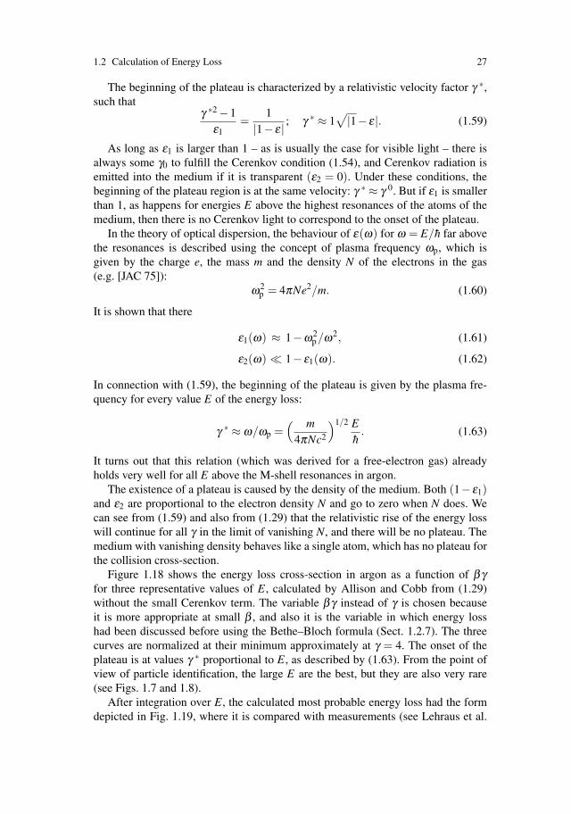
1.2 Calculation of Energy Loss 27
The beginning of the plateau is characterized by a relativistic velocity factor γ ∗,such that
γ ∗2 −1ε1
=1
|1− ε | ; γ ∗ ≈ 1√
|1− ε|. (1.59)
As long as ε1 is larger than 1 – as is usually the case for visible light – there isalways some γ0 to fulfill the Cerenkov condition (1.54), and Cerenkov radiation isemitted into the medium if it is transparent (ε2 = 0). Under these conditions, thebeginning of the plateau region is at the same velocity: γ ∗ ≈ γ 0. But if ε1 is smallerthan 1, as happens for energies E above the highest resonances of the atoms of themedium, then there is no Cerenkov light to correspond to the onset of the plateau.
In the theory of optical dispersion, the behaviour of ε(ω) for ω = E/h far abovethe resonances is described using the concept of plasma frequency ωp, which isgiven by the charge e, the mass m and the density N of the electrons in the gas(e.g. [JAC 75]):
ω2p = 4πNe2/m. (1.60)
It is shown that there
ε1(ω) ≈ 1−ω2p /ω2, (1.61)
ε2(ω) 1− ε1(ω). (1.62)
In connection with (1.59), the beginning of the plateau is given by the plasma fre-quency for every value E of the energy loss:
γ ∗ ≈ ω/ωp =( m
4πNc2
)1/2 Eh
. (1.63)
It turns out that this relation (which was derived for a free-electron gas) alreadyholds very well for all E above the M-shell resonances in argon.
The existence of a plateau is caused by the density of the medium. Both (1− ε1)and ε2 are proportional to the electron density N and go to zero when N does. Wecan see from (1.59) and also from (1.29) that the relativistic rise of the energy losswill continue for all γ in the limit of vanishing N, and there will be no plateau. Themedium with vanishing density behaves like a single atom, which has no plateau forthe collision cross-section.
Figure 1.18 shows the energy loss cross-section in argon as a function of βγfor three representative values of E, calculated by Allison and Cobb from (1.29)without the small Cerenkov term. The variable βγ instead of γ is chosen becauseit is more appropriate at small β , and also it is the variable in which energy losshad been discussed before using the Bethe–Bloch formula (Sect. 1.2.7). The threecurves are normalized at their minimum approximately at γ = 4. The onset of theplateau is at values γ ∗ proportional to E, as described by (1.63). From the point ofview of particle identification, the large E are the best, but they are also very rare(see Figs. 1.7 and 1.8).
After integration over E, the calculated most probable energy loss had the formdepicted in Fig. 1.19, where it is compared with measurements (see Lehraus et al.

28 1 Gas Ionization by Charged Particles and by Laser Rays
Fig. 1.18 Energy dependenceof dE/dx: variation with βγof the energy loss cross-section for Ar at normaldensity, normalized to βγ = 4,according to a calculation byAllison and Cobb [ALL 80].The curves are for threevalues of the energy loss E,corresponding to M-, L-, andK-shell ionization
[LEH 82] and references quoted therein). Both the measured and the calculated val-ues are normalized at γ = 4. The agreement is remarkable and indicates that thetheory gives an adequate explanation of the velocity dependence of gas ionization.
The effect of the gas density on the relativistic rise is visible in the data ofFig. 1.20. There is also a small dependence on the gas sample thickness, for whichwe refer the reader to an article by Walenta [WAL 79] and to Fig. 10.5.
Fig. 1.19 Measured values of the most probable energy loss in an Ar + methane mixture as afunction of βγ , compared with the photo-absorption model of Allison and Cobb for Ar. For details,see [ALL 80] and [LEH 82] and references quoted therein
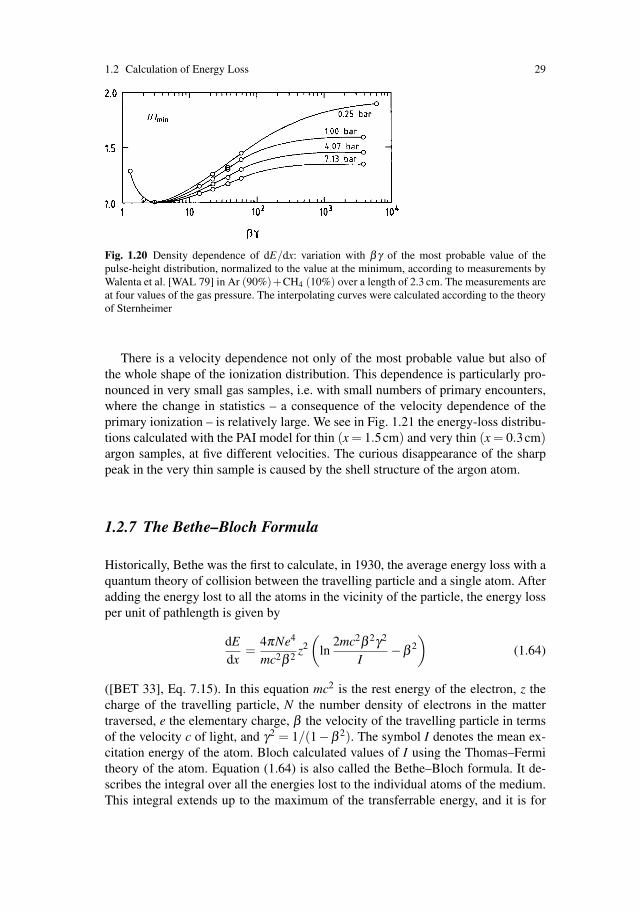
1.2 Calculation of Energy Loss 29
Fig. 1.20 Density dependence of dE/dx: variation with βγ of the most probable value of thepulse-height distribution, normalized to the value at the minimum, according to measurements byWalenta et al. [WAL 79] in Ar (90%)+CH4 (10%) over a length of 2.3 cm. The measurements areat four values of the gas pressure. The interpolating curves were calculated according to the theoryof Sternheimer
There is a velocity dependence not only of the most probable value but also ofthe whole shape of the ionization distribution. This dependence is particularly pro-nounced in very small gas samples, i.e. with small numbers of primary encounters,where the change in statistics – a consequence of the velocity dependence of theprimary ionization – is relatively large. We see in Fig. 1.21 the energy-loss distribu-tions calculated with the PAI model for thin (x = 1.5cm) and very thin (x = 0.3cm)argon samples, at five different velocities. The curious disappearance of the sharppeak in the very thin sample is caused by the shell structure of the argon atom.
1.2.7 The Bethe–Bloch Formula
Historically, Bethe was the first to calculate, in 1930, the average energy loss with aquantum theory of collision between the travelling particle and a single atom. Afteradding the energy lost to all the atoms in the vicinity of the particle, the energy lossper unit of pathlength is given by
dEdx
=4πNe4
mc2β 2 z2(
ln2mc2β 2γ2
I−β 2
)(1.64)
([BET 33], Eq. 7.15). In this equation mc2 is the rest energy of the electron, z thecharge of the travelling particle, N the number density of electrons in the mattertraversed, e the elementary charge, β the velocity of the travelling particle in termsof the velocity c of light, and γ2 = 1/(1−β 2). The symbol I denotes the mean ex-citation energy of the atom. Bloch calculated values of I using the Thomas–Fermitheory of the atom. Equation (1.64) is also called the Bethe–Bloch formula. It de-scribes the integral over all the energies lost to the individual atoms of the medium.This integral extends up to the maximum of the transferrable energy, and it is for
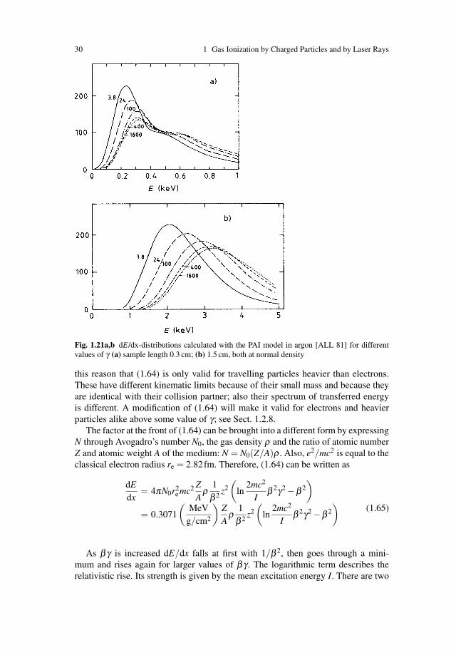
30 1 Gas Ionization by Charged Particles and by Laser Rays
Fig. 1.21a,b dE/dx-distributions calculated with the PAI model in argon [ALL 81] for differentvalues of γ (a) sample length 0.3 cm; (b) 1.5 cm, both at normal density
this reason that (1.64) is only valid for travelling particles heavier than electrons.These have different kinematic limits because of their small mass and because theyare identical with their collision partner; also their spectrum of transferred energyis different. A modification of (1.64) will make it valid for electrons and heavierparticles alike above some value of γ ; see Sect. 1.2.8.
The factor at the front of (1.64) can be brought into a different form by expressingN through Avogadro’s number N0, the gas density ρ and the ratio of atomic numberZ and atomic weight A of the medium: N = N0(Z/A)ρ . Also, e2/mc2 is equal to theclassical electron radius re = 2.82fm. Therefore, (1.64) can be written as
dEdx
= 4πN0r2e mc2 Z
Aρ
1β 2 z2
(ln
2mc2
Iβ 2γ2 −β 2
)
= 0.3071
(MeV
g/cm2
)ZA
ρ1
β 2 z2(
ln2mc2
Iβ 2γ2 −β 2
)(1.65)
As βγ is increased dE/dx falls at first with 1/β 2, then goes through a mini-mum and rises again for larger values of βγ . The logarithmic term describes therelativistic rise. Its strength is given by the mean excitation energy I. There are two

1.2 Calculation of Energy Loss 31
physical origins of this effect. One is in the time behaviour of the electromagneticfield carried by the travelling particle. As seen from the atom, the field componentsof short duration become stronger as γ goes up, increasing the cross-section forthe excitation and ionization. The other reason is kinematic. As βγ is increased themaximal possible energy that can be conveyed from the particle to the atom goes uptoo and makes the average energy increase with βγ . For example, a pion of 1 GeVcan transfer 50 MeV, and a pion of 10 GeV can transfer 3.3 GeV to an electron atrest. Such large energy transfers are not applicable to tracks in drift chambers; thisis another reason for a necessary modification of (1.64); see Sect. 1.2.8.
The mean excitation energy I is calculable for simple atoms, but it has most oftenbeen considered a parameter to be fitted from the measurements of the ionizationenergy loss near the minimum. A critical collection of such determinations of Iis contained in an article by Seltzer and Berger [SEL 82], a selection for relevantdrift chamber gases is presented in our Table 1.5. The mean excitation energy forthe chemical elements is found to increase with the atomic number Z and followsapproximately
I = AZ
with A decreasing from 20 eV (H) to 13 eV (C) and roughly 10 eV (Ar and higher).Values of I for compounds and mixtures can be calculated in a first approximationaccording to Bragg’s additivity rule, which states that
ln Icompound = ∑ni ln Ii/∑ni,
where the ni and Ii are the electron densities and the mean excitation energiesbelonging to element i.
Table 1.5 Mean excitation energies and specific ionization in the minimum for various gases.Values of I from [SEL 82], values of (dE/dx)min/ρ calculated from (1.64′)
Gas Z A Density ρ(N.T.P.)
Mean excitationenergy I
(dE/dx)min/ρ
(g/I) (eV ) (MeV/g cm−2)
Hydrogen H2 1 2.016 0.090 19.2 4.11Helium He 2 4.003 0.178 41.8 1.94Neon Ne 10 20.18 0.90 137 1.73Argon Ar 18 39.95 1.78 188 1.52Krypton Kr 36 83.8 3.74 352 1.36Xenon Xe 54 131.3 5.89 482 1.26Oxygen O2 16 32.00 1.43 95 1.81Nitrogen N2 14 28.01 1.25 82 1.83Methane CH4 10 16.04 0.72 41.7 2.43Ethane C2H6 18 30.07 1.25 45.4 2.31Propane C3H8 26 44.11 1.88 47.1 2.27Isobutane C4H10 34 58.12 2.67 48.3 2.25Ethylene C2H4 20 28.05 1.18 51 2.73Carbon dioxide CO2 22 44.00 1.98 85 1.83

32 1 Gas Ionization by Charged Particles and by Laser Rays
It was discovered later that the relativistic rise would not continue to indefinitelylarge values of γ . In 1939, Fermi calculated the ‘density effect’ as the coherenteffect of the surrounding polarizable atoms, which shield the field of the travellingparticle [FER 40]. A corresponding correction term δ (β ) is introduced into (1.64),which reads in its conventional form
dEdx
=4πNe4
mc2
1β 2 z2
(ln
2mc2
Iβ 2γ2 −β 2 − δ (β )
2
). (1.66)
The exact behaviour of δ (β ) obviously has to depend on the substance and itsstate of aggregation. Sternheimer and others have made parameter descriptions ofδ (β ) which consist of piecewise power-law fits with coefficients derived from theknown oscillator strengths of the relevant substances. Such parameters are tabulatedin [STE 84], and the literature can be traced back from there. Near the minimum,δ = 0, and in the limit of β → 1, the density correction approaches
δ → lnh2ω2
p
I2 γ2 −1 (1.67)
([FAN 63], Eq. 1.49), where hωp is the quantum energy of the plasma oscillationof the medium (see (1.60)). The correction term δ (β )/2 in (1.66), being a linearfunction of ln γ cancels some but not all of the relativistic rise – the dynamic parthas disappeared, and the kinematic part still makes the total energy loss increase,albeit with a smaller rate than before.
1.2.8 Energy Deposited on a Track – Restricted Energy Loss
The track ionization for drift chambers cannot be calculated on the basis of the totalenergy loss described in (1.64). This formula includes all the high-energy transfersthat do not contribute to a track, although they are kinematically possible. Abovea certain energy, an electron knocked out of a gas atom will form a second track,a δ electron, and will not contribute to the first one any more. Above what energythe new track is recognized and its ionization no longer attributed to the first trackdepends on the circumstances. Among these circumstances there is the range (i.e.the length of δ ray until it is stopped) in the particular gas. If the range is below thetypical size of the pick-up electrodes, there is no separation yet. If the range is largecompared to this size, then the second track may be separated by the electronics andthe pattern recognition program. If there is a magnetic field and the track of the δelectron is curved, a similar idea applies to the radius of curvature.
There are also statistical circumstances that produce an effective cut-off: in anyfinite number of measurements there is always one largest energy transfer. A valueof energy transfer so improbable that no track of a given series of measurements,or only an insignificant part of them, contains one is also an effective cut-off. Wehave calculated some examples of cut-off energies in Table 1.6 which result fromthe different effects mentioned above.

1.2 Calculation of Energy Loss 33
Table 1.6 Some energy transfers E relevant for the introduction of an upper cut-off in the definitionof a track of ionization in argon gas
Range of δ electron (bar cm) E (keV)
1 303 6010 12030 250
Radius of curvature of δ -electrontrack in different magnetic fields(cm)
E (MeV)
0.5 in 0.4 T 0.30.5 in 1.5 T 1.85 in 0.4 T 5.55 in 1.5 T 22
Probability of finding one interac-tion with minimum deposit of E on1 bar m of tracklength
E (MeV)
0.1% 121% 1.210% 0.12
Kinematic limits of maximum transferrable energy (MeV)
βγ e π p
0.1 0.001 0.010 0.0101 0.106 1.01 1.024 0.80 15.9 16.310 2.31 95 101100 25.3 5.8×10³ 9.2×10³
1000 255 121×103 490×103
It appears from Table 1.6 that in a typical argon chamber without magnetic fielda cut-off Emax somewhere between 30 and 250 keV is at work on account of therange. Inside a magnetic field the situation is more complicated because some δrays will curl up and stay with the primary track, even up to 1 or several MeV; butthis happens only at the 1% probability level per bar m of tracklength. In summary:there is a cut-off with a value somewhere between 30 keV and 1 MeV (for a typicalargon chamber), depending on the apparatus. It has to replace the kinematic limit ifit is smaller.
The modified Bethe–Bloch formula for the energy loss restricted in this wayreads as follows ([FAN 63], 1.88):

34 1 Gas Ionization by Charged Particles and by Laser Rays
(dEdx
)restricted
=4πNe4
mc2
1β 2 z2
[ln
√2mc2Emaxβγ
I− β 2
2− δ (β )
2
]. (1.68)
Equation (1.68) holds for the range of βγ where Emax is smaller than the kinematiclimit, and for γ2 � Emax/mc2. In comparison to (1.66) the value at the minimum aswell as the relativistic rise have become smaller. Formulae (1.64) and (1.66) werevalid for particles heavier than electrons, because electrons have different kinematiclimits and a different spectrum. The restricted energy loss (1.68) is also applicablefor electrons because the different kinematic limits have been replaced by the com-mon cut-off Emax. It can be shown ([BET 33], Eq. 55.8) that electrons travelling withγ2 � Emax/mc2 produce essentially the same spectrum as heavier particles with thesame γ . The universal validity of (1.68), which implies that the restricted energyloss is a function only of the particle velocity and not of the mass or the energyseparately, is a consequence of the introduction of the cut-off energy Emax.
In the limit β → 1 we now have complete cancellation of the γ dependence, andthe restricted energy loss reaches the ‘Fermi plateau’; insertion of (1.67) into (1.68)yields (
dEdx
)restrβ=1
=4πNe4
mc2 z2 ln
√2mc2Emax
hωp. (1.69)
The ratio between the values of the restricted energy loss on the plateau and in theminimum is given by
R(Emax) =(dE/dx)plateau
restricted
(dE/dx)minimumrestricted
=ln
√2mc2Emax
hωp
ln
√2mc2Emax
I(βγ)min −
β 2min
2
.
(1.70)
If we insert the values of ωp and I for argon gas at N.T.P., using (1.60) andTable 1.5, we obtain R = 1.60, 1.54 and 1.48 for Emax = 30keV, 150keV and 1 MeV,respectively. A precise evaluation of R requires better knowledge of Emax. Whenvarying the gas and its density, Emax will also change in most applications.
The interest in particle identification by ionization measurement brings into focusthe accuracy and hence the statistical aspect. The average energy loss has large fluc-tuations due to rare events with large energy transfer. Therefore the most probableenergy loss is a better estimator.
The analytic method of Landau for the determination of the most probable energyloss cannot be a basis for the calculation of the energy dependence of ionizationin drift chambers – their gas layers are too thin, and the cut-off required by thedefinition of a track is not part of Landau’s method.
A statistical formulation of the problem, treated with Monte–Carlo methodsalong the lines of Ermilova, Kotenko and Merzon [ERM 77] or of Allison and

1.2 Calculation of Energy Loss 35
Cobb [ALL 80], is better suited to describing the velocity dependence of the mostprobable energy loss. The properties of the medium enter into these models throughthe frequency dependence of the dielectric constant, which in turn is derivable fromexperimental photoabsorption coefficients. We have presented the photoabsorptionionization model [PAI] of Allison and Cobb in Sect. 1.2.2. Some more informa-tion including numerical values of the energy loss from the PAI model on theFermi plateau is contained in Chap. 10. A step-by-step comparison of the methodof Bethe–Bloch–Sternheimer with the PAI model does not exist, to our knowledge.
The reader who is interested in more historical details may find useful the famousold book by Rossi [ROS 52]. An in-depth discussion of ionization is contained inthe monograph by Bugadov, Merson, Sitar and Chechin [BUG 88] as well as in thearticle by Fano [FAN 63].
1.2.9 Localization of Charge Along the Track
As we have seen in Sects. 1.1.1 and 1.2.2, the charge along a track is created indiscrete clusters that vary greatly in size. This has some consequence for the coor-dinate measurement of the track. The precise way in which the discrete nature ofionization determines fundamental limits of accuracy depends on the measurementmethod in question and will be dealt with in Chap. 7. In preparation, we discusshere the following question: Given a certain track length L – for example, the partof the track collected onto one wire – with what precision is the centre of gravity ofthe discretely deposited ionization located along the track? If the coordinate alongthe track is x, and in the ith cluster we have ni electrons, then the centre of gravityis at
x =m
∑i=1
(xini)/ m
∑i=1
ni. (1.71)
Let the track extend around 0 from −L/2 to +L/2. The probability distribution forevery xi is
f (xi) dxi = (1/L) dxi. (1.72)
Averaging over all xi, we have for every fixed set of ni
〈x〉 = 0
and
〈x2〉 =
⟨m
∑i=1
x2i n2
i
⟩/(m
∑i=1
ni
)2
(1.73)
=L2
12
m
∑i=1
n2i
/(m
∑i=1
ni
)2
=L2
121
Neff.
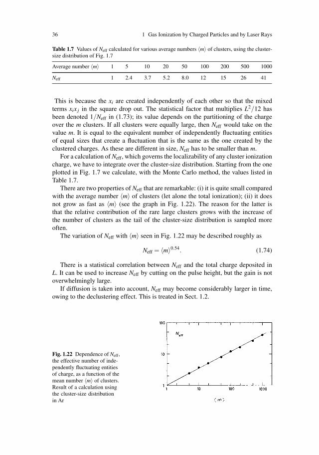
36 1 Gas Ionization by Charged Particles and by Laser Rays
Table 1.7 Values of Neff calculated for various average numbers 〈m〉 of clusters, using the cluster-size distribution of Fig. 1.7
Average number 〈m〉 1 5 10 20 50 100 200 500 1000
Neff 1 2.4 3.7 5.2 8.0 12 15 26 41
This is because the xi are created independently of each other so that the mixedterms xix j in the square drop out. The statistical factor that multiplies L2/12 hasbeen denoted 1/Neff in (1.73); its value depends on the partitioning of the chargeover the m clusters. If all clusters were equally large, then Neff would take on thevalue m. It is equal to the equivalent number of independently fluctuating entitiesof equal sizes that create a fluctuation that is the same as the one created by theclustered charges. As these are different in size, Neff has to be smaller than m.
For a calculation of Neff, which governs the localizability of any cluster ionizationcharge, we have to integrate over the cluster-size distribution. Starting from the oneplotted in Fig. 1.7 we calculate, with the Monte Carlo method, the values listed inTable 1.7.
There are two properties of Neff that are remarkable: (i) it is quite small comparedwith the average number 〈m〉 of clusters (let alone the total ionization); (ii) it doesnot grow as fast as 〈m〉 (see the graph in Fig. 1.22). The reason for the latter isthat the relative contribution of the rare large clusters grows with the increase ofthe number of clusters as the tail of the cluster-size distribution is sampled moreoften.
The variation of Neff with 〈m〉 seen in Fig. 1.22 may be described roughly as
Neff = 〈m〉0.54. (1.74)
There is a statistical correlation between Neff and the total charge deposited inL. It can be used to increase Neff by cutting on the pulse height, but the gain is notoverwhelmingly large.
If diffusion is taken into account, Neff may become considerably larger in time,owing to the declustering effect. This is treated in Sect. 1.2.
Fig. 1.22 Dependence of Neff,the effective number of inde-pendently fluctuating entitiesof charge, as a function of themean number 〈m〉 of clusters.Result of a calculation usingthe cluster-size distributionin Ar

1.2 Calculation of Energy Loss 37
1.2.10 A Measurement of Neff
The effective number of independently fluctuating charges along the length L of atrack can be measured. The r.m.s. fluctuation of the centre of gravity of the chargedeposited along L is, by definition of Neff, equal to
δyc =L√
12Neff.
A particle track whose ionization is sampled over a length L by n wires withpulse heights Pi(i = 1, . . . ,n) has the centre of its charge at
yc = ∑Piyi/∑Pi,
where the yi are the wire positions along the track. A measurement of yc of manytracks allows a determination of δyc, and hence of Neff, to be made.
In an experiment using a model of the ALEPH TPC, cosmic-ray tracks werecollected in a small interval of momentum and angle of incidence. The chambercontained an Ar (90%)+CH4(10%) gas mixture at atmospheric pressure and had asense-wire spacing of 0.4 cm. Track lengths L between 0.8 and 20 cm were specifiedand Neff was calculated for every L. The result is shown in Fig. 1.23. The choiceof L is limited on the low side by the wire spacing and on the high side by thedynamic range of the pulse-height recording. In the case under consideration, theoverflow bin contained 1.5% of the pulses. For higher values of L this bin is sampledmore often, and the calculated number Neff begins to depend on the details of anextrapolation of the overflow bin. A power-law fit to Fig. 1.23 shows that Neff variedwith L according to
Neff ∝ (L/1cm)0.45±0.1.
Comparing Figs. 1.22 and 1.23, we notice that the exponent is identical, withinerrors, to that obtained from the theoretical cluster-size distribution. Using the powerlaw, which is only an empirical relation, we may obtain an estimate of the primaryionization density, because it can be expected that the function Neff(L) becomesequal to 1 at L = λ, the average distance between clusters.
Fig. 1.23 Neff measured withcosmic rays as a functionof the track length L. Thelast data point has the largestdependence on the treatmentof the overflow bin (see text).The three values correspondto extrapolation accordingto (a) a 1/PH2 law, (b) theLandau distribution or (c) noextrapolation, respectively
38 1 Gas Ionization by Charged Particles and by Laser Rays
1.3 Gas Ionization by Laser Rays
The light of a narrow pulsed laser beam that traverses a volume of gas, underfavourable conditions, is capable of ionizing the gas in the beam so that it imitatesa straight particle track. For this to occur, there must be some ionizable moleculesin the gas, and the energy density must be sufficiently high, depending on the wave-length. In practice, a small nitrogen laser, emitting pulses of 104 W on a few squaremillimetres at λ = 337nm, may be sufficient in an ordinary chamber gas that has notbeen especially cleansed and therefore contains suitable molecules in some low con-centration. This technique has the obvious advantage of producing identical tracksin the same place. Therefore, by taking repeated measurements of the same coor-dinate, one may form the average, which can be made almost free from statisticalvariations, if only the number of repeated measurements is made large enough. Inpractice 100 shots are usually sufficient. The technique has been widely used eversince its first application in 1979 [AND 79].
Chemical compounds used for laser ionization are discussed in Sect. 12.4.
1.3.1 The nth Order Cross-Section Equivalent
The quantum energy of laser light in the visible and the near ultraviolet is muchlower than the ionization energies of molecules. It takes two or more such laserphotons to ionize the organic molecules present in the chamber gas. Multiphotonionization processes involving 11 photons have been observed in xenon (see thereview by Lambropoulos [LAM 76]). For the ionization of a molecule to occur, then photons have to be incident on the molecule during the lifetime of the intermediatestates. Then the ionization rate varies the nth power of the photon flux becausethe photons act incoherently in the gas. The probability of n photons arriving ina given time interval is equal to the nth power of the probability of each one ofthem, and is therefore proportional to the nth power of the photon flux φ . Just as theconcept of ‘cross-section’ σ describes one-particle collision rates in units of cm2,we have an ‘nth-order cross-section equivalent’ σ (n) for n-particle collisions in unitsof cm2nsn−1. In a volume V containing a density N of molecules, the ionization rateR is therefore given by the expression
R = φ n NV σ (n). (1.75)
In fact, n-photon ionization is most easily identified by a measurement of R as afunction of φ .
A light pulse with cross-sectional area A and duration T contains m photons ifthe flux φ and the energy E are given by
φ = m/(AT ),
E = mhν = mhc/λ.
1.3 Gas Ionization by Laser Rays 39
Considering a traversed volume V = AL, the specific ionization per unit track lengthfor the n-photon process is
RTL
=mn
(AT )n−1 Nσ (n)
=(
EAT
)n
AT N
(λhc
)n
σ (n).
(1.76)
In (1.76), (E/AT ) is the power density of the beam.So far, we have implicitly assumed the duration of the light pulse to be short
compared with the inverse transition frequencies between the states involved. Themore general situation develops towards a dynamic equilibrium between excitationand de-excitation. The case of two-photon ionization is treated in more detail inSect. 1.3.2.
The molecular ions created in the ionization do not as a rule resemble the par-ent molecules very much, because they are cracked in the process. Fragmentationpatterns are complicated and usually not understood [REI 85].
1.3.2 Rate Equations for Two-Photon Ionization
For the electrons in the molecules, we distinguish the ground level (0), the inter-mediate level (1), and the continuum ionization level (2). We denote the populationdensities in the gas by P0, P1, and P2. The incident radiation stimulates transitions0 → 1, 1 → 2, and 1 → 0, but there are also spontaneous transitions 1 → 0. Depend-ing on the circumstances, there may be losses from level 1 into other channels. Thetransition rates, denoted by k1 to k4, are determined by the incident flux and by theinternal transition mechanism.
The rate equations are written in the following form (the primes denote the timederivatives):
P′0(t) = −k1P0(t)+(k1 + k2)P1(t),
P′1(t) = +k1P0(t)− (k1 + k2 + k3 + k4)P1(t),
P′2(t) = k4P1.
(1.77)
They are symbolized in Fig. 1.24.The rate per molecule k1 is taken to be proportional to the incoming flux φ of pho-
tons; the constant of proportionality is the cross-section σ01 for the process 0 → 1:
k1 = σ01φ . (1.78)
We want to calculate the transition rate P′2(t) with which electrons appear in the
continuum state. It is proportional to the density P1(t) of the intermediate state, andthe corresponding rate per molecule is
k4 = σ12φ . (1.79)

40 1 Gas Ionization by Charged Particles and by Laser Rays
Fig. 1.24 Scheme of thefive transition rates used in(1.77a–c)
The first two of the rate equations are a system of homogeneous linear differentialequations. Before we derive the general mathematical solution, we shall considersome limiting cases in order to better understand the physical content of (1.77).
Before the pulse arrives, P0(0) is of the order of 1013 per cubic centimetre in agas having a typical concentration of the ionizing molecules of one part per million,and P1(0) = 0. While P1(t) is slowly built up at the rate P′
1(t), we may considerP0 as a constant as long as P1(t) has not developed into a similar order of magni-tude. The situation of making only a few ionization electrons with the laser shot iswell described by this approximation, which treats the ground state as an infinitereservoir.
(a) Case of P0 as an Infinite Reservoir. We may write the first two of (1.77) in thefollowing form:
P′0(t) = −k1P0 +(k1 + k2)P1(t), (1.80a)
P′1(t) = +k1P0 − (k1 + k2 + k3 + k4)P1(t). (1.80b)
The solution of (1.80b) is
P1(t) =k1P0
∑k(1− e−t ∑k), (1.81)
where ∑k = k1 + k2 + k3 + k4. Obviously, our approximation is always fulfilled ifk1 ∑k or σ01φ ∑k (using (1.78)). Let us assume that this is the case. Equa-tion (1.81) leads to a production rate of ionization equal to
P′2(t) = k4P1(t) =
k1k4P0
∑k(1− e−t ∑k). (1.82)
Integrated over the duration T of a constant light pulse, the total density reached atthe end of the pulse is given by

1.3 Gas Ionization by Laser Rays 41
P2(T ) =k1k4P0
∑k
[T − (1− e−T ∑k)
/∑k]. (1.83)
In the limit of short pulses, i.e. T 1/∑k, the exponential may be expanded tosecond order and gives us
P2(T ) → 12
k1k4P0T 2. (1.84)
In the limit of long pulses, i.e. T � 1/∑k, the exponential vanishes, so that
P2(T ) → k1k4P0
∑kT. (1.85)
Expression (1.84) is proportional to φ 2, the square of the photon flux, because of(1.78) and (1.79). This is also the case for expression (1.85) unless k1 or k2 domi-nates ∑k. In our approximation that treats P0 as an infinite reservoir, we assume thatk1 ∑k; then a similar condition holds for k2 (except for special circumstances inwhich σ12 is orders of magnitude larger than σ10):
P2(T ) → 12
σ01σ12P0φ 2T 2 (small T, small φ), (1.86)
P2(T ) → σ01σ12
k2 + k3P0φ 2T (large T, small φ). (1.87)
(b) General Case. If we want to know what happens when the photon flux is strong,(1.77) have to be solved in a rigorous way. This is achieved by a variabletransformation that separates the equations (see any textbook on differentialequations, for example [KAM 59].) One finds the eigenvalues s1,s2 of the ma-trix of coefficients from the determinant
∣∣∣∣−k1 − s k1 + k2
k1 −∑k− s
∣∣∣∣= 0, (1.88)
s1,2 = −∑k + k1
2±[(
∑k + k1
2
)2
− k1(k3 + k4)
]1/2
. (1.89)
These two eigenvalues are real and negative; we take s2 < s1 < 0.The solutions to the differential equations (1.77) satisfying the initial conditions
P1(0) = 0,P2(0), are given by
P0(t) =P0(0)s1 − s2
[−(k1 + s2)es1t +(k1 + s1)es2t ], (1.90a)
P1(t) =P0(0)k1
s1 − s2[es1t − es2t ], (1.90b)
P2(t) =P0(0)k1k4
s1s2
[1+
s2
s1 − s2es1t − s1
s1 − s2es2t]. (1.90c)
42 1 Gas Ionization by Charged Particles and by Laser Rays
Equation (1.90c) represents the general solution to the problem. It describes theconcentration of ionization electrons as a function of time and of the rate coefficientsk1 to k4. For small t we recover our expressions (1.84) and (1.86) by developing theexponentials to the second order in s1t and s2t:
P2(t) →12
k1k4P0(0)t2. (1.91)
For large t, using (1.89), we obtain
P2(t) →k4
k3 + k4P0(0). (1.92)
This enormous concentration of electrons (saturation) would imply that the groundstate has been emptied, a situation that should not concern us when we study ion-ization tracks that are similar to particle tracks.
Equation (1.91), identical to (1.84) and (1.86), gives rise to the definition of thesecond-order cross-section equivalent described in Sect. 1.3.1. For a laser shot ofduration T , identifying R/V with P2/T , we have
σ (2) =12
σ01σ12T. (1.93)
Under the conditions that lead to (1.87), we have instead
σ (2) = σ01σ12/(k2 + k3), (1.94)
whereas under the most general conditions, including saturation, σ (2) depends notonly on T but also on φ .
1.3.3 Dependence of Laser Ionization on Wavelength
The ionization yield depends very much on the wavelength. Using tunable dyelasers, Ledingham and co-workers have found an increase of four orders of mag-nitude, when going from λ = 330nm to λ = 260nm. In Fig. 1.25 ‘clean’ countergas is compared with a gas seeded with a small amount of phenol. The finestructure visible around 270 nm was resolved using high-resolution techniquesand was compared with the known single-photon UV absorption of phenol(see Fig. 1.26).
The identical wavelength dependence is apparent. We understand this behaviourfrom (1.93) and (1.94): the wavelength dependence resides almost entirely in thefactor σ01, implying that the cross-section for ionization from the intermediate leveldoes not vary so much. The amount of characteristic structure in the spectrum oflaser-induced resonant two-photon ionization (‘R2PI’) makes it a sensitive tool forthe identification of molecules [HUR 79].

1.3 Gas Ionization by Laser Rays 43
Fig. 1.25 Ionization induced in untreated counter gas [Ar (90%)+CH4(10%)] by a 1×1mm2
pulsed laser beam of 1μJ(×), compared with the same gas seeded with a small amount of phenol(+) [TOW 86]
Fig. 1.26 A comparison of the laser-induced R2PI spectrum of counter gas doped with a trace ofphenol (B) and the single-photon UV absorption spectrum of phenol [TOW 86]

44 1 Gas Ionization by Charged Particles and by Laser Rays
1.3.4 Laser-Beam Optics
A beam of laser light that is to create ionization as if from a particle must have anapproximately constant cross-sectional area along the beam. Relations (1.75) and(1.76) imply that, for example, in two-photon ionization a light pulse with a givenenergy produces half as many ions per unit track length when it has twice the cross-sectional area. In the interest of a constant high yield and of a narrow deposit ofionization, one would like to have the beam width as small as possible over thelargest possible track length.
The photons in a beam occupy a volume in the four-dimensional phase spaceat each point along the beam. For illustration, we consider the horizontal plane inFig. 1.27, where an almost parallel beam is shown to be focused into a narrowwaist by a lens. After the focus, the beam opens up again. Each photon trajectoryis represented by a point in the phase-space diagrams below where the distancefrom the axis is plotted against the small angle of the trajectory with the axis. Herewe deal with geometrical optics only; the wave optical aspects are treated later. Inthis sense we may regard the optical elements of the beam (lenses, mirrors, lightguides, free space, apertures) as determining a trajectory for each photon in a time-independent fashion. Now, Liouville’s theorem in statistical mechanics states thatin such a passive system the density of photons in phase space is a constant ofmotion, meaning that it does not change along the beam. As long as there are nophotons lost, the occupied volume of cross-sectional area times solid angle is thesame everywhere along the beam and the same as just behind the laser. In the phase-space diagrams of Fig. 1.27 the envelopes containing the beam do not change theirarea. A concentration of the beam in space by a focusing lens is accompanied by acorresponding extension of the solid angle.
Fig. 1.27 Phase-space diagrams at three points along a light-beam, which is almost parallel at theleft and is focussed into B by a lens at A
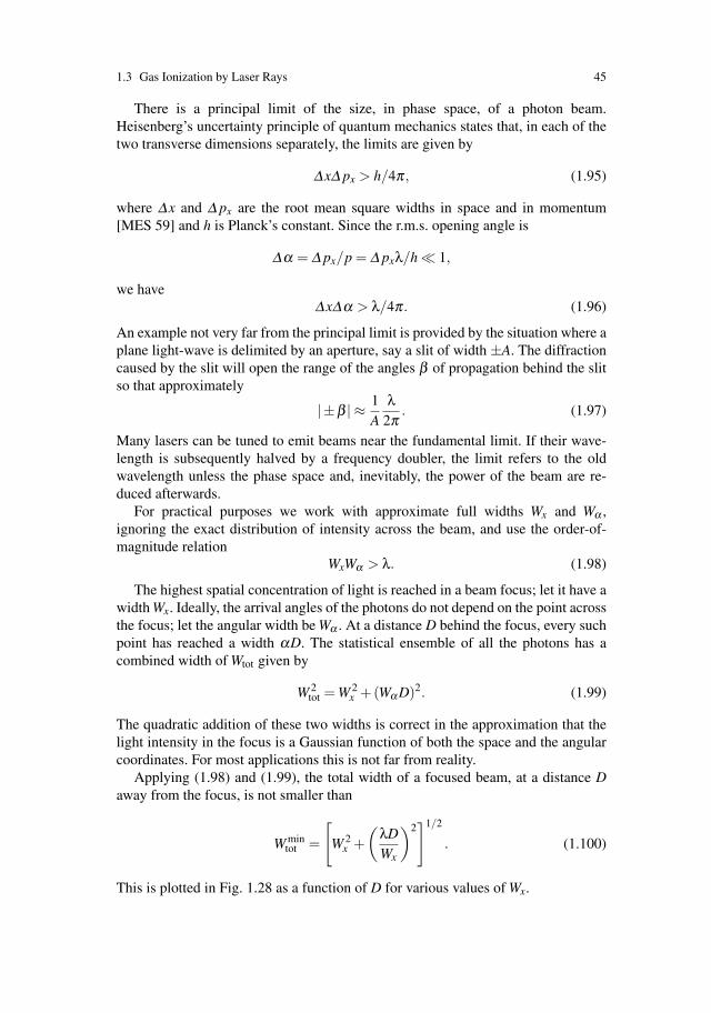
1.3 Gas Ionization by Laser Rays 45
There is a principal limit of the size, in phase space, of a photon beam.Heisenberg’s uncertainty principle of quantum mechanics states that, in each of thetwo transverse dimensions separately, the limits are given by
ΔxΔ px > h/4π, (1.95)
where Δx and Δ px are the root mean square widths in space and in momentum[MES 59] and h is Planck’s constant. Since the r.m.s. opening angle is
Δα = Δ px/p = Δ pxλ/h 1,
we haveΔxΔα > λ/4π. (1.96)
An example not very far from the principal limit is provided by the situation where aplane light-wave is delimited by an aperture, say a slit of width ±A. The diffractioncaused by the slit will open the range of the angles β of propagation behind the slitso that approximately
|±β | ≈ 1A
λ2π
. (1.97)
Many lasers can be tuned to emit beams near the fundamental limit. If their wave-length is subsequently halved by a frequency doubler, the limit refers to the oldwavelength unless the phase space and, inevitably, the power of the beam are re-duced afterwards.
For practical purposes we work with approximate full widths Wx and Wα ,ignoring the exact distribution of intensity across the beam, and use the order-of-magnitude relation
WxWα > λ. (1.98)
The highest spatial concentration of light is reached in a beam focus; let it have awidth Wx. Ideally, the arrival angles of the photons do not depend on the point acrossthe focus; let the angular width be Wα . At a distance D behind the focus, every suchpoint has reached a width αD. The statistical ensemble of all the photons has acombined width of Wtot given by
W 2tot = W 2
x +(Wα D)2. (1.99)
The quadratic addition of these two widths is correct in the approximation that thelight intensity in the focus is a Gaussian function of both the space and the angularcoordinates. For most applications this is not far from reality.
Applying (1.98) and (1.99), the total width of a focused beam, at a distance Daway from the focus, is not smaller than
W mintot =
[W 2
x +(
λDWx
)2]1/2
. (1.100)
This is plotted in Fig. 1.28 as a function of D for various values of Wx.
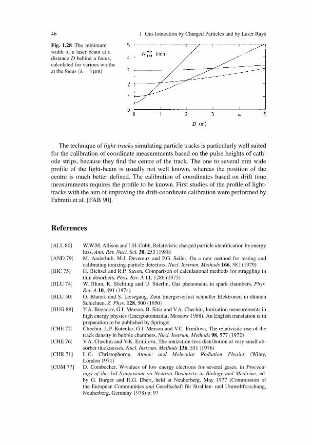
46 1 Gas Ionization by Charged Particles and by Laser Rays
Fig. 1.28 The minimumwidth of a laser beam at adistance D behind a focus,calculated for various widthsat the focus (λ = 1μm)
The technique of light-tracks simulating particle tracks is particularly well suitedfor the calibration of coordinate measurements based on the pulse heights of cath-ode strips, because they find the centre of the track. The one to several mm wideprofile of the light-beam is usually not well known, whereas the position of thecentre is much better defined. The calibration of coordinates based on drift timemeasurements requires the profile to be known. First studies of the profile of light-tracks with the aim of improving the drift-coordinate calibration were performed byFabretti et al. [FAB 90].
References
[ALL 80] W.W.M. Allison and J.H. Cobb, Relativistic charged particle identification by energyloss, Ann. Rev. Nucl. Sci. 30, 253 (1980)
[AND 79] M. Anderhub, M.J. Devereux and P.G. Seiler, On a new method for testing andcalibrating ionizing-particle detectors, Nucl. Instrum. Methods 166, 581 (1979)
[BIC 75] H. Bichsel and R.P. Saxon, Comparison of calculational methods for straggling inthin absorbers, Phys. Rev. A 11, 1286 (1975)
[BLU 74] W. Blum, K. Sochting and U. Stierlin, Gas phenomena in spark chambers, Phys.Rev. A 10, 491 (1974)
[BLU 50] O. Blunck and S. Leisegang, Zum Energieverlust schneller Elektronen in dunnenSchichten, Z. Phys. 128, 500 (1950)
[BUG 88] Y.A. Bugadov, G.I. Merson, B. Sitar and V.A. Chechin, Ionization measurements inhigh energy physics (Energoatomizdat, Moscow 1988). An English translation is inpreparation to be published by Springer
[CHE 72] Chechin, L.P. Kotenko, G.I. Merson and V.C. Ermilova, The relativistic rise of thetrack density in bubble chambers, Nucl. Instrum. Methods 98, 577 (1972)
[CHE 76] V.A. Chechin and V.K. Ermilova, The ionization-loss distribution at very small ab-sorber thicknesses, Nucl. Instrum. Methods 136, 551 (1976)
[CHR 71] L.G. Christophorou, Atomic and Molecular Radiation Physics (Wiley,London 1971)
[COM 77] D. Combecher, W-values of low energy electrons for several gases, in Proceed-ings of the 3rd Symposium on Neutron Dosimetry in Biology and Medicine, ed.by G. Burger and H.G. Ebert, held at Neuherberg, May 1977 (Commission ofthe European Communities and Gesellschaft fur Strahlen- und Umweltforschung,Neuherberg, Germany 1978) p. 97
References 47
[ERM 69] V.K. Ermilova, L.P. Kotenko, G.I. Merzon and V.A. Chechin, Primary specificionization of relativistic particles in gases, Sov. Phys.-JETP 29, 861 (1969)
[ERM 77] V.K. Ermilova, L.P. Kotenko and G.I. Merzon, Fluctuations and the most probablevalues of relativistic charged particle energy loss in thin gas layers, Nucl. Instrum.Methods 145, 555 (1977)
[FAB 90] R. Fabretti, M. Fabre, L. Li, P. Razis, P.G. Seiler and O. Prokofiev, Relation betweenthe lateral distribution of UV laser induced ionization in a drift chamber and theshape of the corresponding signal, Nucl. Instr. Meth. Phys. Res. A 287, 413 (1990)
[FAN 63] U. Fano, Penetration of protons, alpha particles and mesons, Ann. Rev. Nucl. Sc. 13,1 (1963)
[FER 40] E. Fermi, The ionization loss of energy in gases and in condensed materials, Phys.Rev. 57, 485 (1940)
[FIS 91] H. Fischle, J. Heintze and B. Schmidt, Experimental determination of ioniza-tion cluster size distributions in counting gases, Nucl. Instrum. Methods A 301,202 (1991)
[HAR 73] F. Harris, T. Katsura, S. Parker, V.Z. Peterson, R.W. Ellsworth, G.B. Yodh, W.W.M.Allison, C.B. Brooks, J.H. Cobb and J.H. Mulvey, The experimental identificationof individual particles by the observation of transition radiation in the X-ray region,Nucl. Instrum. Methods 107, 413 (1973)
[HUR 79] G.S. Hurst, M.G. Payne, S.D. Kramer and J.P. Young, Resonance ionization spectro–scopy and one-atom detection, Rev. Mod. Phys. 51, 767 (1979)
[INO 75] M. Inokuti, Ionization yields in gases under electron irradiation, Radiat. Res. 64,6 (1975)
[INT 79] International Commission on Radiation Units and Measurements, Average energyrequired to produce an ion pair (ICRU Report 31, Washington, DC, 1979)
[JAC 75] J.D. Jackson, Classical electrodynamics, 2nd edn (Wiley, New York 1975)[KAM 59] E. Kamke, Differentialgleichungen, Losungsmethoden und Losungen, 6th edn
(Akademische Verlagsgesellschaft, Leipzig 1959)[KOB 68] E.J. Kobetich and R. Katz, Energy deposition by electron beams and delta rays,
Phys. Rev. 170, 391 (1968)[KOL 84] K.S. Kolbig and B. Schorr, A program package for the Landau distribution, Comput.
Phys. Commun. 31, 97 (1984)[LAM 76] P. Lambropoulos, Topics in multiphoton processes in atoms, Adv. At. and Mol. Phys.
12, 87 (1976)[LAN 44] L.D. Landau, On the energy loss of fast particles by ionization, J. Phys. USSR 8, 201
(1944). Also in Collected Papers of L.D. Landau, ed. by D. Ter Haar (Pergamon,Oxford 1965)
[LAN 60] L.D. Landau and E.M. Lifshitz, Electrodynamics of Continuous Media, Vol. 8 ofCourse of Theoretical Physics (Pergamon, Oxford 1960) p. 84
[LAP 80] F. Lapique and F. Piuz, Simulation of the measurement by primary cluster countingof the energy lost by a relativistic ionizing particle in argon, Nucl. Instrum. Methods175, 297 (1980)
[LEH 78] I. Lehraus, R. Matthewson, W. Tejessy and M. Aderholz, Performance of a large-scale multilayer ionization detector and its use for measurements of the relativisticrise in the momentum range of 20–110 GeV/c, Nucl. Instrum. Methods 153,347 (1978)
[LEH 82] I. Lehraus, R. Matthewson and W. Tejessy, Particle identification by dE/dx samplingin high-pressure drift detectors, Nucl. Instrum. Methods 196 (1982) 361
[MAR 76] G.V. Marr and J.B. West, Absolute photoionization cross-section tables for helium,neon, argon and krypton in the VUV spectral regions, At. Data and Nucl. DataTables 18, 497 (1976)
[MES 59] A. Messiah, Mecanique Quantique (Dunod, Paris 1959)[PRO 74] Proc. Symp. on the Jesse Effect and Related Phenomena, Gatlinburg (Tenn.), 1973
[Radiat. Res. 59, 337 (1974)]

48 1 Gas Ionization by Charged Particles and by Laser Rays
[RIE 72] F.F. Rieke and W. Prepejchal, Ionization cross-sections of gaseous atoms andmolecules for high-energy electrons and positrons, Phys. Rev. A 6, 1507 (1972)
[REI 85] H. Reisler and C. Wittig, Multiphoton ionization of gaseous molecules, in Photodis-sociation and Photoionization, ed. by K.P. Lawley (Wiley, New York 1985)
[ROS 52] B. Rossi, High-energy Particles (Prentice-Hall, Englewood Cliffs, NJ 1952)[SEL 82] S.M. Seltzer and M.J. Berger, Evaluation of the stopping power of elements
and compounds for electrons and positrons, Int. J. Appl. Radiation Isotope 33,1189 (1982)
[SOC 79] K. Sochting, Measurement of the specific primary excitation of helium and neon byfast charged particles, Phys. Rev. A 20, 1359 (1979)
[STE 84] R.M. Sternheimer, M.J. Berger and S.M. Seltzer, Density effect for the ionizationloss of charged particles in various substances, At. Data and Nucl. Data Tables 30,261 (1984)
[STE 71] R.M. Sternheimer and R.F. Peierls, General expression for the density effect for theionization loss of charged particles, Phys. Rev. B 3, 3681 (1971)
[TOW 86] M. Towrie, J.W. Cahill, K.W.D. Ledingham, C. Raine, K.M. Smith, M.H.C. Smith,D.T.S. Stewart and C.M. Houston, Detection of phenol in proportional-counter gasby two-photon ionisation spectroscopy, J. Physics B (At. Mol. Phys.) 19, 1989 (1986)
[VAV 57] P.V. Vavilov, Ionization losses of high-energy heavy particles, Sov. Phys. JETP 5,749 (1957)
[WAL 79] A.H. Walenta, J. Fischer, H. Okuno and C.L. Wang, Measurement of the ionizationloss in the region of relativistic rise for noble and molecular gases, Nucl. Instrum.Methods 161, 45 (1979)
[WAL 81] A.H. Walenta, Performance and development of dE/dx counters, Phys. Scr. 23,354 (1981)
Chapter 2The Drift of Electrons and Ions in Gases
The behaviour of the drift chamber is crucially dependent on the drift of theelectrons and ions that are created by the particles measured or in the avalanchesat the electrodes. In addition to the electric drift field, there is often a magnetic field,which is necessary for measuring particle momentum. Obviously we have to under-stand how the drift velocity vector in electric and magnetic fields depends on theproperties of the gas molecules, including their density and temperature. We mightstart by writing down the most general expression and then specialize to simplepractical cases. However, it is more ‘anschaulich’ to proceed in the opposite way.We derive the simple cases first and then generalize to the more rigorous formulationin Sect. 2.3.
2.1 An Equation of Motion with Friction
The motion of charged particles under the influence of electric and magnetic fields,E and B may be understood in terms of an equation of motion:
mdu
dt= eE + e[u×B]−Ku, (2.1)
where m and e are the mass and electric charge of the particle, u is its velocity vector,and K describes a frictional force proportional to u that is caused by the interactionof the particle with the gas. In Sect. 2.2 we will see that in terms of the more detailedtheory involving atomic collisions, (2.1) describes the drift at large t to a very goodapproximation. Historically, (2.1) was introduced by P. Langevin, who imagined theforce Ku as a stochastic average over the random collisions of the drifting particle.
The ratio m/K has the dimension of a characteristic time, and we define
τ =mK
. (2.2)
Equation (2.1) is an inhomogeneous system of linear differential equations for thethree components of velocity.
W. Blum et al., Particle Detection with Drift Chambers, 49doi: 10.1007/978-3-540-76684-1 2, c© Springer-Verlag Berlin Heidelberg 2008

50 2 The Drift of Electrons and Ions in Gases
The solution for t � τ of (2.1) is a steady state for which du/dt = 0. The driftvelocity vector is determined by the linear equation
1τu− e
m[u×B] =
em
E. (2.3)
In order to solve for u, we write (e/m)Bx = ωx etc., (e/m)Ex = εx, etc., andexpress (2.3) in the form of the matrix equation
Mu = ε ,
M =
⎡⎣ 1/τ −ωz ωy
ωz 1/τ −ωx
−ωy ωx 1/τ
⎤⎦ .
(2.4)
The solution is obtained by inverting M:
u = M−1ε ,
M−1 =
⎡⎣ 1+ω2
x τ2 ωzτ +ωxωyτ2 −ωyτ +ωxωzτ2
−ωzτ +ωxωyτ2 1+ω2y τ2 ωxτ +ωyωzτ2
ωyτ +ωxωzτ2 −ωxτ +ωyωzτ2 1+ω2z τ2
⎤⎦
× τ1+ω2τ2 , (2.5)
where ω2 = ω2x +ω2
y +ω2z = (e/m)2 B2 is the square of the cyclotron frequency of
the electron. As we explain in Sect. 2.3, our solution (2.5) is equal to that obtainedin the full microscopic theory in the approximation that τ is independent of thecollision energy [see the discussion following (2.84)].
A different way of writing (2.5) is the following:
u =em
τ |E| 11+ω2τ2 (E +ωτ [E× B]+ω2τ2(E · B)B). (2.6)
Here E and B denote the unit vectors in the directions of the fields. The drift di-rection is governed by the dimensionless parameter ωτ , where ω is defined as(e/m)|B| and carries the sign of the charge of the moving particle.
For ωτ = 0, u is along E; in this case the relation has the simple form
u =em
τE = μE,
μ =em
τ.(2.7)
These equations define the scalar mobility μ as the ratio of drift velocity to electricfield in the absence of magnetic field; μ is proportional to the characteristic time τdefined in (2.2) and carries the charge sign of the particle.
In the presence of the magnetic field, the mobility is the tensor (e/m)M−1 givenin (2.5). For large positive values of ωτ and e > 0, u generally tends to be along B;but if E · B = 0, then large ω τ turn u in the direction of E× B, independently of

2.1 An Equation of Motion with Friction 51
the sign of e. Reversing the magnetic field direction causes the E × B componentin (2.6) to change sign. Reversing the charge of the particle causes the E and the(E · B)B components in (2.6) to change sign.
An illustration of the directional behaviour of u is presented in Fig. 2.1a, wherethe coordinate system is oriented so that the z axis is along B, and E is in the x–zplane. A positively charged particle starting at the origin will arrive on the plane z0
at a point which belongs to a half circle over the diameter connecting the end-pointsof the B and E vectors in the z0 plane. This is so because the components of u inthese coordinates satisfy the relation
(ux
uz− 1
2Ex
Ez
)2
+(
uy
uz
)2
=(
12
Ex
Ez
)2
for any ωτ . The component in the direction of E × B is largest for ωτ = 1. Inpractice one studies primarily the drift of electrons; their negative electric chargecauses a drift behaviour with respect to the E and B fields, which is illustrated inFig. 2.1b [DYD 04].
Both the direction and the magnitude of u are influenced by the magnetic field.If we distinguish u(ω), the drift velocity in the presence of B, and u(0), the driftvelocity at B = 0 under otherwise identical circumstances, using (2.6) we derive
u2(ω)u2(0)
=1+ω2τ2 cos2 φ
1+ω2τ2 , (2.8)
where φ is the angle between E and B. This ratio happens to be the same as theone by which the component of u along E, uE , changes with B:
uE(ω)uE(0)
=1+ω2τ2 cos2 φ
1+ω2τ2 . (2.9)
z = 0z = 0
z = 0z = z 0
z = 0z = - z 0
z = 0z = 0
a b
1
0
inf.
–1
0 –inf.
EB
B E
z
y
x
x
y
x
y
z
x
y
Fig. 2.1 Directional behaviour of the drift velocity of a particle in the presence of an electric anda magnetic field. Values of the parameter ωτ are indicated along the half-circle on the z0 plane:(a) case of positive electric charge of the particle; (b) case of negative charge

52 2 The Drift of Electrons and Ions in Gases
2.1.1 Case of E Nearly Parallel to B
Two cases are of special interest. The first applies to the situation where a magneticfield is almost parallel to the electric field. Using (2.6) with E = (0, 0, Ez),B =(Bx, By, Bz), and |Bx|, |By| |Bz|, we express the drift directions in first order by
ux
uz=
−ωτBy +ω2τ2Bx
(1+ω2τ2)Bz,
uy
uz=
ωτBx +ω2τ2By
(1+ω2τ2)Bz.
(2.10)
Here the terms proportional to ωτ/(1 + ω2τ2) change sign under a reversal ofB [go back to (2.6) in order to see this]. Equations (2.10) will be used in Sect. 2.4.4for the analysis of track distortions.
2.1.2 Case of E Orthogonal to B
The second case of interest applies to the situation where E is at right angles to B.Using (2.6) with (E · B) = 0, E = (Ex, 0, 0), and B = (0, 0, Bz), we have
ux =(e/m)τ
1+ω2τ2 |E|,
uy = − (e/m)τ1+ω2τ2 ωτ |E|,
uz = 0,
tanψ ≡ uy
ux= −ωτ.
(2.11)
From (2.11) we deduce the following for the magnitude of u:
|u| = (e/m)τ√1+ω2τ2
|E| = em
τ |E|cosψ. (2.12)
The product |E|cosψ represents the component of the electric field in the driftdirection. Compared with the magnetic-field-free case (2.7), we may write the func-tional dependence on |E| and |B| in the following form:
|u| = F(E,B) = F(E cosψ,0), (2.13)
which is also known as Tonks’ theorem [TON 55].The expression has a simple meaning: regardless of the drift direction of the
electron, the component of the electric field along this direction determines the driftvelocity for every magnetic field. The derivation of (2.13) is based on a constantvalue of τ and is experimentally verified to good precision (see Fig. 2.26). This isdiscussed in more detail in Sects. 2.2.3 and 2.4.6.
2.2 The Microscopic Picture 53
2.2 The Microscopic Picture
On the microscopic scale, the electrons or ions that drift through the gas are scat-tered on the gas molecules so that their direction of motion is randomized in eachcollision. On average, they assume a constant drift velocity u in the direction of theelectric field E (or, if a magnetic field is also present, in the direction which is givenby both fields). The drift velocity u is much smaller than the instantaneous velocityc between collisions.
The gases we deal with are sufficiently rarefied that the distances travelled byelectrons between collisions are large in comparison with their Compton wave-lengths. So our picture is classical and atomistic. For gas pressures above, say,100 atm, slow-drifting electrons interact with several atoms simultaneously and re-quire a quantum mechanical treatment [BRA 81, ATR 77].
In order to understand the drift mechanism, we derive some basic relationsbetween the macroscopic quantities of drift velocity u and isotropic diffusion co-efficient D on the one hand and the microscopic quantities of electron velocityc, mean time τ between collisions, and fractional energy loss λ on the other. Themicroscopic quantities are randomly distributed according to distribution functionstreated in Sect. 2.3; in this section we deal with suitable averages. The relevant re-lations can be expected to be correct within factors of the order of unity.
2.2.1 Drift of Electrons
Let us consider an electron between two collisions. Because of its light mass, theelectron scatters isotropically and, immediately after the collision, it has forgottenany preferential direction. Some short time later, in addition to its instantaneous andrandomly oriented velocity c, the electron has picked up the extra velocity u equalto its acceleration along the field, multiplied by the average time that has elapsedsince the last collision:
u =eEm
τ. (2.14)
This extra velocity appears macroscopically as the drift velocity. In the next en-counter, the extra energy, on the average, is lost in the collision through recoil orexcitation. Therefore there is a balance between the energy picked up and the colli-sion losses. On a drift distance x, the number of encounters is n = (x/u)(1/τ), thetime of the drift divided by the average time τ between collisions. If λ denotes theaverage fractional energy loss per collision, the energy balance is the following:
xuτ
λεE = eEx. (2.15)
Here the equilibrium energy εE carries an index E because it does not contain thepart due to the thermal motion of the gas molecules, but only the part taken out ofthe electric field.

54 2 The Drift of Electrons and Ions in Gases
One may wonder about the fact that the average time between collisions is thesame as the average time that has elapsed since the last collision. This is becausein a completely random series of encounters, characterized only by the average rate1/τ , the differential probability f (t)dt that the next encounter is a time between tand t +dt away from any given point t = 0 in time is
f (t)dt =1τ
e−t/τ dt, (2.16)
independent of the point where the time measurement begins.Equation (2.14), as compared with (2.7), provides an interpretation and a justifi-
cation of the constant τ introduced in Sect. 2.1. In the frictional-motion picture, τwas the ratio of the mass of the drifting particle over the coefficient of friction. Inthe microscopic picture, τ is the mean time between the collisions of the driftingparticle with the atoms of the gas. For drifting particles with instantaneous velocityc, the mean time τ between collisions may be expressed in terms of the cross-sectionσ and the number density N:
1τ
= Nσc. (2.17)
Here c is related to the total energy of the drifting electron by
12
mc2 = ε = εE +32
kT, (2.18)
because the total energy is made up of two parts: the energy received from theelectric field and the thermal energy that is appropriate for 3 degrees of freedom(k = Boltzmann’s constant, T = gas temperature).
For electron drift in particle detectors, we usually have εE � (3/2)kT ; we canneglect the thermal motion, and (2.14), (2.15), and (2.18) combine to give the twoequilibrium velocities as follows:
u2 =eE
mNσ
√λ2, (2.19)
c2 =eE
mNσ
√2λ
, (2.20)
where ε = (1/2)mc2 � εE � (3/2)kT .Both σ and λ are functions of ε . (We are confident that the fractional energy loss
per collision, λ, Eq. 2.15, will not be confused with a mean free path or a wavelengthwhich are traditionally also called λ). One notices the important role played by theenergy loss in the collisions: with vanishing λ, the drift velocity would becomezero. If ε is below the excitation levels of the gas molecules, the scattering is elasticand λ is approximately equal to twice the mass ratio of the collision partners (seeSect. 2.2.2); hence it is of the order of 10−4 for electrons.
As an illustration, we show in Fig. 2.2a the behaviour of the effective cross-sections for argon and methane, two typical counter gases used in drift chambers.
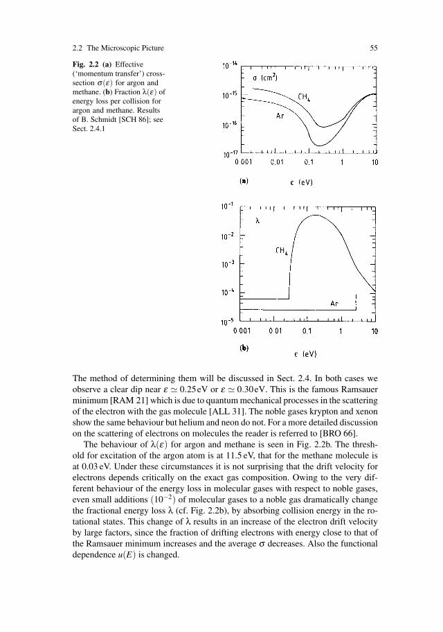
2.2 The Microscopic Picture 55
Fig. 2.2 (a) Effective(‘momentum transfer’) cross-section σ(ε) for argon andmethane. (b) Fraction λ(ε) ofenergy loss per collision forargon and methane. Resultsof B. Schmidt [SCH 86]; seeSect. 2.4.1
The method of determining them will be discussed in Sect. 2.4. In both cases weobserve a clear dip near ε � 0.25eV or ε � 0.30eV. This is the famous Ramsauerminimum [RAM 21] which is due to quantum mechanical processes in the scatteringof the electron with the gas molecule [ALL 31]. The noble gases krypton and xenonshow the same behaviour but helium and neon do not. For a more detailed discussionon the scattering of electrons on molecules the reader is referred to [BRO 66].
The behaviour of λ(ε) for argon and methane is seen in Fig. 2.2b. The thresh-old for excitation of the argon atom is at 11.5 eV, that for the methane molecule isat 0.03 eV. Under these circumstances it is not surprising that the drift velocity forelectrons depends critically on the exact gas composition. Owing to the very dif-ferent behaviour of the energy loss in molecular gases with respect to noble gases,even small additions (10−2) of molecular gases to a noble gas dramatically changethe fractional energy loss λ (cf. Fig. 2.2b), by absorbing collision energy in the ro-tational states. This change of λ results in an increase of the electron drift velocityby large factors, since the fraction of drifting electrons with energy close to that ofthe Ramsauer minimum increases and the average σ decreases. Also the functionaldependence u(E) is changed.
56 2 The Drift of Electrons and Ions in Gases
We note that the dependence of the drift velocity and the electron energy on Eand N is always through the ratio E/N. This implies that in two gases operated withdifferent gas pressures and identical temperature, the E fields must be adjusted inproportion to the gas pressures in order to obtain identical u and ε in both gases.Reduced fields are given in units of V cm−1 Torr−1. A special unit has also beencoined: one Townsend (1 Td) is 10−17 V cm2.
In a gas mixture composed of two or more components i with number densitiesni, the effective cross-section σ(ε) and the effective fractional energy loss per colli-sion λ(ε) have to be calculated from the properties of the individual components:
σ(ε) = ∑niσi(ε)/N,
λ(ε)σ(ε) = ∑niλi(ε)σi(ε)/N, (2.21)
N = ∑ni.
The general behaviour of electron drift velocities is that they rise with increasingelectric field, then level off or decrease as a result of the combined effects of σ(ε)and λ(ε) as ε increases with increasing E. Examples will be presented in Sect. 2.4and in Chap. 12.
2.2.2 Drift of Ions
The behaviour of ions differs from that of electrons because of their much larger massand their chemical reactions. The monograph by McDaniel and Mason[MCD 73] deals with the mobility and diffusion of ions in gases in a comprehen-sive way. Electrons in an electric field are accelerated more rapidly than ions, andthey lose very little energy when colliding elastically with the gas atoms. The electronmomentum is randomized in the collisions and is therefore lost, on the average. Inelectric field strengths that are typical for drift chambers, the electrons reach randomenergies far in excess of the energy of the thermal motion, and quite often they surpassthe threshold of inelastic excitation of molecules in the gas. In this case their mobilitybecomes a function of the energy loss that is associated with such excitation.
Ions in similar fields acquire, on one mean-free path, an amount of energy thatis similar to that acquired by electrons. But a good fraction of this energy is lost inthe next collision, and the ion momentum is not randomized as much. Therefore, farless field energy is stored in random motion. As a consequence, the random energyof ions is mostly thermal, and only a small fraction is due to the field. The effecton the diffusion of ions results in this diffusion being orders of magnitude smallerthan that of electrons in similar fields. The effect on the mobility is also quite inter-esting: since the energy scale, over which collision cross-sections vary significantly,is easily covered by the electron random energies reached under various operatingconditions, we find rapid and sometimes complicated dependences of electron mo-bility on such operating conditions – electric and magnetic field strengths and gascomposition being examples. In contrast, the mobility of ions does not vary as much.
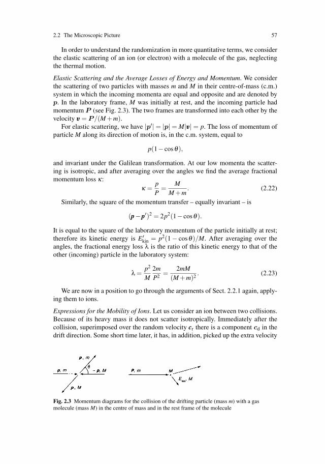
2.2 The Microscopic Picture 57
In order to understand the randomization in more quantitative terms, we considerthe elastic scattering of an ion (or electron) with a molecule of the gas, neglectingthe thermal motion.
Elastic Scattering and the Average Losses of Energy and Momentum. We considerthe scattering of two particles with masses m and M in their centre-of-mass (c.m.)system in which the incoming momenta are equal and opposite and are denoted byp. In the laboratory frame, M was initially at rest, and the incoming particle hadmomentum P (see Fig. 2.3). The two frames are transformed into each other by thevelocity vvv = P /(M +m).
For elastic scattering, we have |p′| = |p| = M|vvv| = p. The loss of momentum ofparticle M along its direction of motion is, in the c.m. system, equal to
p(1− cosθ),
and invariant under the Galilean transformation. At our low momenta the scatter-ing is isotropic, and after averaging over the angles we find the average fractionalmomentum loss κ:
κ =pP
=M
M +m. (2.22)
Similarly, the square of the momentum transfer – equally invariant – is
(p−p′)2 = 2p2(1− cosθ).
It is equal to the square of the laboratory momentum of the particle initially at rest;therefore its kinetic energy is E ′
kin = p2(1 − cosθ)/M. After averaging over theangles, the fractional energy loss λ is the ratio of this kinetic energy to that of theother (incoming) particle in the laboratory system:
λ =p2
M2mP2 =
2mM(M +m)2 . (2.23)
We are now in a position to go through the arguments of Sect. 2.2.1 again, apply-ing them to ions.
Expressions for the Mobility of Ions. Let us consider an ion between two collisions.Because of its heavy mass it does not scatter isotropically. Immediately after thecollision, superimposed over the random velocity cr there is a component cd in thedrift direction. Some short time later, it has, in addition, picked up the extra velocity
Fig. 2.3 Momentum diagrams for the collision of the drifting particle (mass m) with a gasmolecule (mass M) in the centre of mass and in the rest frame of the molecule
58 2 The Drift of Electrons and Ions in Gases
v equal to the acceleration of the ion along the field, multiplied by the average timethat has elapsed since the last collision. The drift velocity is the sum of v and cd:
u = vvv +cd =eEm
τ +cd. (2.24)
The value of cd is given by the average momentum loss in the direction of thedrift that takes place in the next encounter; it must be equal to the momentum mvpicked up between the encounters:
κm〈cr +cd +vvv〉 = κm(cd +vvv) = mvvv, (2.25)
where the brackets 〈 〉 denote the average over the angles. For the magnitude of cd
we calculate cd = v(1−κ)/κ , and for the drift velocity (using (2.22)),
u = v + cd =v
κ=
em
Eτ1κ
=em
Eτ(
1+mM
). (2.26)
Here τ is given by the relative velocity crel between the ion and the gas molecule,the cross-section σ , and the number density N as
1τ
= Nσcrel. (2.27)
We now distinguish two limiting cases of field strength E. If it is low so that theion random velocity is thermal, we must take for the relative velocity the averagemagnitude of the difference between the two randomly distributed velocities of theion (cion) and the gas atoms (cgas):
crel = 〈|cion −cgas|〉 = (c2ions + c2
gas)1/2. (2.28)
With equipartition of energy, we can express crel through the temperature T andBoltzmann’s constant k:
c2rel = c2
ion + c2gas = 3kT
(1m
+1M
). (2.29)
Using (2.26, 2.27), and (2.29), we obtain
u =(
1m
+1M
)1/2( 13kT
)1/2 eENσ
(low E). (2.30)
It is characteristic of the drift velocity at low fields that it is proportional to E, orthat the mobility is independent of E.
For the case of large E, where we can neglect the thermal motion, we pro-ceed as in the case of electrons (where the temperature was always neglected). Bycombining (2.15, 2.17, 2.24), and (2.26), we solve for u2 and c2 and obtain thesymmetric forms

2.2 The Microscopic Picture 59
u2 =eE
m∗Nσ
(λ2
mm∗
)1/2
(2.31)
and
c2 =eE
m∗Nσ
(2λ
mm∗
)1/2
, (2.32)
where the ‘reduced mass’ m∗ between the ion (m) and the gas molecule (M) isdefined as
1m∗ =
1m
+1M
. (2.33)
Using (2.23), we may express λ for elastic scattering through the ratio of the masses,with the result that
u =[
eEmNσ
]1/2 [mM
(1+
mM
)]1/2(high E). (2.34)
It is characteristic of the drift velocity at high fields and constant cross-section σthat it is proportional to the square root of E, or the mobility decreases as 1/
√E.
The distinction between ‘high’ and ‘low’ E in (2.30) and (2.34) is obviously withrespect to the field in which the ion, over one mean free path, picks up an amountof energy equal to the thermal energy. The measured ion drift velocities for noblegases shown in Fig. 2.4 exhibit very well the limit in behaviour of (2.30) and (2.34)with the electric field.
Table 2.1 contains ion mobilities for low fields that were measured in the noblegases. Various approximation methods for the calculation of cross-sections in thescattering of ions on molecules have been treated elsewhere [MCD 73]. When ionstravel in their parent gas, the original collision cross-section is increased by about afactor of two by the mechanism of resonant charge transfer.
Ion Drift in Gas Mixtures. The gas of a drift chamber is often a composition of twoor more constituents. Ion drift in gas mixtures can be understood along the lines ofthe last subsection. We want to modify (2.26) for the case where one type of ion(mass m) moves between the atoms or molecules with masses Mk(k = 1,2, . . .) eachpresent in the gas with its own number density Nk. The gas number density N isequal to the sum over all the Nk. The resulting drift velocity in the field E is calledu; it is equal to
u =em
E τ1κ
. (2.35)
Here τ is the mean time between collisions, and κ is the mean fractional momentumloss in the mixture; they are both quickly calculated from the τk and κk that belongto each constituent. The overall collision rate is the sum of the individual collisionrates, or
1/τ = ∑(1/τk). (2.36)
The overall momentum loss is the average over all the κk, weighted with the relativerates with which each type of molecule is bombarded:
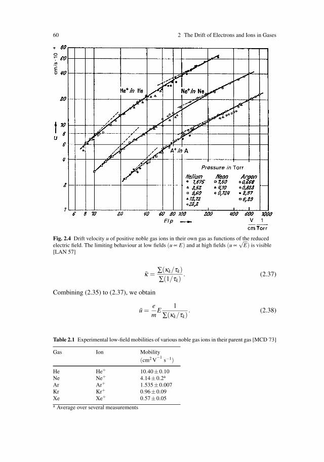
60 2 The Drift of Electrons and Ions in Gases
Fig. 2.4 Drift velocity u of positive noble gas ions in their own gas as functions of the reducedelectric field. The limiting behaviour at low fields (u ∝ E) and at high fields (u ∝
√E) is visible
[LAN 57]
κ = ∑(κk/τk)∑(1/τk)
. (2.37)
Combining (2.35) to (2.37), we obtain
u =em
E1
∑(κk/τk). (2.38)
Table 2.1 Experimental low-field mobilities of various noble gas ions in their parent gas [MCD 73]
Gas Ion Mobility
(cm2 V−1
s−1)
He He+ 10.40±0.10Ne Ne+ 4.14±0.2a
Ar Ar+ 1.535±0.007Kr Kr+ 0.96±0.09Xe Xe+ 0.57±0.05a Average over several measurements

2.2 The Microscopic Picture 61
This equation can be cast into a form that is known as Blanc’s law if we denote byuk the drift velocity of the ion in the pure component k at the full density N:
uk =em
Eτk
κk
Nk
N, (2.39)
where we have used (2.17). Expressions (2.38) and (2.39) give us Blanc’s law:
1u
= ∑ Nk
N1uk
; (2.40)
it states that the inverse drift velocities in the individual gas components add inproportion to the relative component densities to yield the inverse drift velocity ofthe mixture.
Blanc’s law holds for the case of low electric fields. The case of high fields isslightly more complicated because the energy partition of the drifting ion into ran-dom and directed motion must be taken into account. The reader is referred to themonograph of McDaniel and Mason [MCD 73].
In practice, (2.40) is quite well fulfilled. In Fig. 2.5 we show mobilities, mea-sured by the Charpak group [SCH 77], as functions of the relative gas concentrationfor several binary mixtures of argon with the common quench gases: isobutane,methane, and carbon dioxide.
Fig. 2.5 The inverse of themobility of the positivemolecular ions as a func-tion of the relative volumeconcentration of the two com-ponents in three gas mixture.Measurements by [SCH 77]

62 2 The Drift of Electrons and Ions in Gases
The production of positive ions in molecular gases is a fairly complex phe-nomenon, and without a clear identification – perhaps using a mass spectrometer –one is usually ignorant of the identity of the migrating charged bodies. For the pur-poses of drift chambers it often suffices to know their drift velocities. However, thechemical deposits on the wire electrodes, as a result of chamber operation, can beevaluated with more complete knowledge about which ions really migrate towardthe cathodes.
One must read Table 2.2, which contains measured ion mobilities, with theseremarks in mind. For example, the notation ‘[(OCH3)2CH2]
+’ means the ion(s) trav-elling towards the cathode in a mixture of argon + methylal. It is assumed here thatthe argon ions that are created simultaneously transfer their charge to the methylalmolecules, thus creating more ‘[(OCH3)2CH2]
+’ ions. This is elaborated below.
Charge Transfer. When the migrating ions in a drift chamber collide with moleculesthat have an ionization potential smaller than the energy available in the ion, there isthe possibility that a charge-exchange process takes place, which neutralizes the ionand creates a new ion. This process happens with cross-sections that are of a similarorder of magnitude to the other ion–molecule scattering cross-sections. Thereforethe rate of ion transformation through charge transfer is correspondingly high andproportional to the concentration of the molecules to be ionized.
The Charpak group have found that 1% of methylal added to binary argon +isobutane mixtures made a significant change in the ion mobility over 2 cm of drift intheir field (a few hundred to a thousand V/cm). This has to be interpreted as a chargetransfer process from the ions in the original mixture to the methylal molecules,thus creating ‘[(OCH3)2CH2]+’ ions with lesser mobility. Their result [SCH 77] ispresented in Fig. 2.6, where the inverse measured mobility is plotted against the den-sity of the various binary and ternary mixtures. Straight lines correspond to Blanc’slaw; they connect mixtures in which the migrating ion(s) is (are) supposedly thesame. We must therefore imagine the motion of ions in drift chambers as a dynamicprocess in which the various ionic species, which were originally produced in theavalanches or any other collision process, disappear quickly and leave only the onetype that has the lowest ionization potential.
Table 2.2 Measured mobilities of various ions in some gases used in drift chambers [SCH 77]
Ion notation Gas Mobility
(cm2 V−1
s−1)
[CH4]+ Ar 1.87[CO2]+ Ar 1.72[IsoC4H10]+ Ar 1.56[(OCH3)2CH2]
+ Ar 1.51[CH4]+ CH4 2.26[CO2]+ CO2 1.09[IsoC4H10]+ IsoC4H10 0.61[(OCH3)2CH2]
+ IsoC4H10 0.55[(OCH3)2CH2]
+ (OCH3)2CH2 0.26
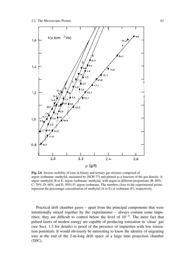
2.2 The Microscopic Picture 63
Fig. 2.6 Inverse mobility of ions in binary and ternary gas mixture composed ofargon–isobutane–methylal, measured by [SCH 77] and plotted as a function of the gas density. A:argon–methylal; B to E: argon–isobutane–methylal, with argon in different proportions (B: 80%,C: 70%, D: 60%, and E: 50%) F: argon–isobutane. The numbers close to the experimental pointsrepresent the percentage concentration of methylal (A to E) or isobutane (F), respectively
Practical drift chamber gases – apart from the principal components that wereintentionally mixed together by the experimenter – always contain some impu-rities; they are difficult to control below the level of 10−4. The mere fact thatpulsed lasers of modest energy are capable of producing ionization in ‘clean’ gas(see Sect. 1.3 for details) is proof of the presence of impurities with low ioniza-tion potentials. It would obviously be interesting to know the identity of migratingions at the end of the 2-m-long drift space of a large time projection chamber(TPC).
64 2 The Drift of Electrons and Ions in Gases
2.2.3 Inclusion of Magnetic Field
When we consider the influence of a magnetic field on drifting electrons andions, the first indication may be provided by the value of the mobility μ of thesecharges. In particle chamber conditions, this is of the order of magnitude of μ �104 cm2 V
−1s−1 for electrons (see Fig. 2.17 and use (2.7)), whereas for ions the
order of magnitude is μ = 1cm2 V−1
s−1 (see Tables 2.1 and 2.2). Typical magneticfields B available to particle experimenters are limited, so far, by the magnetic sus-ceptibility of iron, and the order of magnitude is 1 T or 10−4 V s cm−2. We knowfrom Sect. 2.1 that it is the numerical value of ωτ = (e/m)Bτ that governs the ef-fects of the magnetic field on the drift velocity vector. Using (2.7), which stated thatμ = (e/m)τ , we find
ωτ = Bμ �{
10−4 for ions
1 for electrons
in order of magnitude. Therefore, the effect of such magnetic fields on ion drift isnegligible, and we concentrate on electrons. This has the advantage that we mayassume that the colliding body scatters isotropically in all directions, owing to itssmall mass.
When the magnetic field is added to the considerations of Sect. 2.2.1, we candescribe the most general case in a coordinate system in which B is along z, and Ehas components Ez and Ex. An electron between collisions moves according to theequation of motion,
mdvvvdt
= eE + e[vvv×B], (2.41)
which in our case is written as
vx = εx +ωvy,
vy = −ωvx,
vz = εz,
(2.42)
where ω ≡ (e/m)B and ε ≡ (e/m)E. Electrons have their direction of motion ran-domized in each collision, and we are interested in the extra velocity picked up bythe electron since the last collision. Hence we look for the solution of (2.42) withvvv = 0 at t = 0. It is given by
vx(t) = (εx/ω)sin ωt,
vy(t) = (εx/ω)(cos ωt −1),
vx(t) = εzt.
(2.43)
Before we can identify v with the drift velocity, we must average over t, using (2.16),the probability distribution of t. This was also done when deriving (2.14), which,being a linear function of time, required t to be replaced by τ , the mean time sincethe last collision. The drift velocity for the present case is given by

2.2 The Microscopic Picture 65
ux = 〈vx(t)〉 =εx
ω
∞∫0
1τ
e−t/τ sin ωt dt =εxτ
1+ω2τ2 ,
uy = 〈vy(t)〉 =εx
ω
∞∫0
1τ
e−t/τ(cos ωt −1)dt =−εxωτ2
1+ω2τ2 , (2.44)
uz = 〈vz(t)〉 = εz
∞∫0
1τ
e−t/τ dt = εzτ .
We immediately recognize that the result is the same as for (2.5) and (2.6), de-rived from the macroscopic equation of motion using the concept of friction. Themobility tensor (2.5) is therefore the same in the macroscopic and the microscopicpicture. It will only have to be modified in Sect. 2.3, where the electron velocity hasa probability distribution over a range of values, rather than a single value.
We can now state the condition of energy balance in the presence of a magneticfield. If the angle between the two fields is φ , the energy transferred to the electronper unit distance along E, equal to the corresponding collision loss, is
eE =12
λmc2
uE(ω)τ=
12
λm2c2(1+ω2τ2)eEτ2(1+ω2τ2 cos2 φ)
. (2.45)
Here we have used (2.9). On the other hand, the square of the drift velocity wasgiven by (2.7) and (2.8),
u2 =( e
mEτ)2 1+ω2τ2 cos2 φ
1+ω2τ2 . (2.46)
The two expressions (2.45) and (2.46) determine the two equilibrium velocities uand c. First we notice that the ratio
u2
c2 =λ2
(2.47)
is given by the fractional energy loss per collision alone; in particular, it is inde-pendent of both fields. In the situation without magnetic field, the two electronvelocities were determined by the cross-section and the energy loss in (2.19) and(2.20). With magnetic field, the corresponding relations are more complicated ow-ing to the presence of the terms proportional to ω2τ2 = ω2/(N2σ2c2). Whereas inthe most general case (2.45) and (2.46) could be solved for c2 by a graphical ornumerical method, we present the closed solution for two important practical cases.
Case of E Parallel to B. The first case concerns the drift volume of the TPC; herewe have cos2 φ = 1 and therefore
c2 eEmNσ
√2λ
, (2.48)
exactly as in the absence of magnetic field.
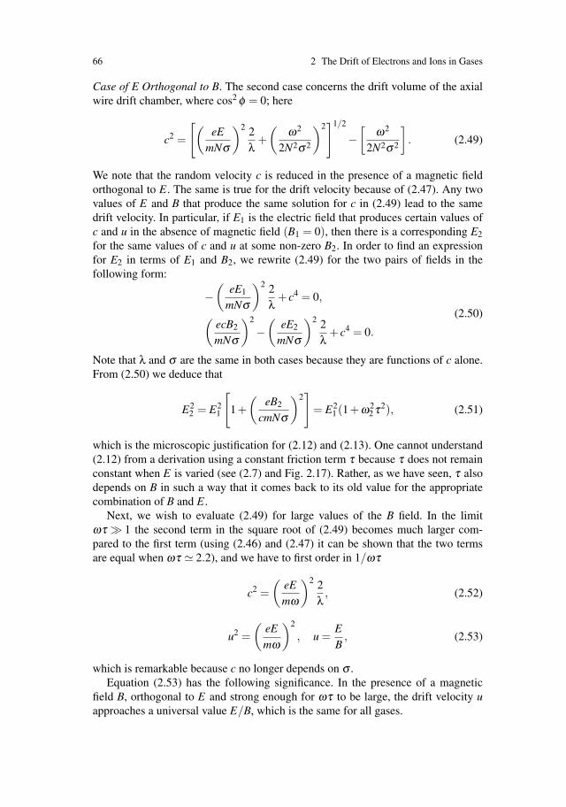
66 2 The Drift of Electrons and Ions in Gases
Case of E Orthogonal to B. The second case concerns the drift volume of the axialwire drift chamber, where cos2 φ = 0; here
c2 =
[(eE
mNσ
)2 2λ
+(
ω2
2N2σ2
)2]1/2
−[
ω2
2N2σ2
]. (2.49)
We note that the random velocity c is reduced in the presence of a magnetic fieldorthogonal to E. The same is true for the drift velocity because of (2.47). Any twovalues of E and B that produce the same solution for c in (2.49) lead to the samedrift velocity. In particular, if E1 is the electric field that produces certain values ofc and u in the absence of magnetic field (B1 = 0), then there is a corresponding E2
for the same values of c and u at some non-zero B2. In order to find an expressionfor E2 in terms of E1 and B2, we rewrite (2.49) for the two pairs of fields in thefollowing form:
−(
eE1
mNσ
)2 2λ
+ c4 = 0,
(ecB2
mNσ
)2
−(
eE2
mNσ
)2 2λ
+ c4 = 0.
(2.50)
Note that λ and σ are the same in both cases because they are functions of c alone.From (2.50) we deduce that
E22 = E2
1
[1+(
eB2
cmNσ
)2]
= E21 (1+ω2
2 τ2), (2.51)
which is the microscopic justification for (2.12) and (2.13). One cannot understand(2.12) from a derivation using a constant friction term τ because τ does not remainconstant when E is varied (see (2.7) and Fig. 2.17). Rather, as we have seen, τ alsodepends on B in such a way that it comes back to its old value for the appropriatecombination of B and E.
Next, we wish to evaluate (2.49) for large values of the B field. In the limitωτ � 1 the second term in the square root of (2.49) becomes much larger com-pared to the first term (using (2.46) and (2.47) it can be shown that the two termsare equal when ωτ � 2.2), and we have to first order in 1/ωτ
c2 =(
eEmω
)2 2λ
, (2.52)
u2 =(
eEmω
)2
, u =EB
, (2.53)
which is remarkable because c no longer depends on σ .Equation (2.53) has the following significance. In the presence of a magnetic
field B, orthogonal to E and strong enough for ωτ to be large, the drift velocity uapproaches a universal value E/B, which is the same for all gases.

2.2 The Microscopic Picture 67
In order to study the deviations from the universal expression (2.53), we maycarry the expansion of the square root in (2.49) to the second order. Using (2.47)and (2.53) we find
u =EB
(1− 1
ω2τ2
)(ωτ � 1). (2.54)
This means that the universal limit (2.53) is approached rapidly from below as B isincreased.
This physical content of (2.53) can best be understood by comparison with themotion of an electron in vacuo: under the influence of crossed electric and magneticfields, the electron is accelerated by the E field and bent by the B field; it performsa cycloidal motion in the plane orthogonal to B (see (2.43) and Fig. 2.7). Whenaveraging over the periodic part, one finds that the electron drifts with the constantspeed E/B in the direction of −E × B. This motion in vacuo is the limit of thegas drift for large values of ωτ , the mean number of turns (expressed in radians)between collisions. Experimentally it can be reached either by increasing the B fieldor by reducing the gas density, which is roughly proportional to 1/τ .
2.2.4 Diffusion
As the drifting electrons or ions are scattered on the gas molecules, their drift ve-locity deviates from the average owing to the random nature of the collisions. In thesimplest case the deviation is the same in all directions, and a point-like cloud of
Fig. 2.7 Motion of an elec-tron in vacuo under theinfluence of orthogonal Eand B fields: B goes out of thepaper, the electron stays in theplane of the paper

68 2 The Drift of Electrons and Ions in Gases
electrons which then begins to drift at time t = 0 from the origin in the z directionwill, after some time t, assume the following Gaussian density distribution:
n =(
1√4πDt
)3
exp
(−r2
4Dt
), (2.55)
where r2 = x2 + y2 + (z− ut)2; D is the diffusion constant because n satisfies thecontinuity equation for the conserved electron current Γ :
Γ = nu−D∇n, (2.56)
∂n∂ t
+∇ ·Γ = 0, (2.57)
∂n∂ t
+n∇ ·u−D∇2n = 0. (2.58)
The diffusion constant D, defined by (2.56), makes the mean squared deviation ofthe electrons equal to 2Dt in any one direction from their centre. (This is a specialcase of (2.75), which deals with the case of anisotropic diffusion.)
In order to express the diffusion constant in terms of the microscopic picture, wesuppose that one electron or ion starts at time t = 0 and has a velocity c; hence,according to (2.16), there is probability distribution of free path l equal to
g(l)dl =1l0
e−l/l0dl, (2.59)
where l0 = cτ is the mean free path. The simplest case is the one where scatteringis isotropic with respect to the drift direction. We consider this case first. It appliesto ions at low electric fields E(E/(Nσ) kT ) and, to a good first approximation,to electrons.
Consider a time t at which a large number, n, of encounters have already oc-curred; then n = t/τ . The mean square displacement in one direction, say x, is
∫ ( n
∑1
li cosθi
)2 n
∏1
g(lk)dlkd cosθk
2= n
23
l20 =
23
l20
τt. (2.60)
Hence li cosθi is the displacement along x between the (i− 1)th and the ith colli-sion (Fig. 2.8); the cosθi are uniformly distributed between −1 and +1 accordingto our assumption. The li are distributed with the probability density (2.59). Notethat the mixed terms in the sum vanish. The part proportional to 2t is the diffusioncoefficient D,
D =l20
3τ=
cl03
=c2τ3
=23
εm
τ. (2.61)
Recalling the expression for the electron mobility μ ,
μ =em
τ,

2.2 The Microscopic Picture 69
Fig. 2.8 Electron paths forthe derivation of (2.60)
we notice that the electron energy can be determined by a measurement of theratio D/μ :
ε =32
Deμ
. (2.62)
When the diffusing body has thermal energy, ε = (3/2)kT , (2.62) takes the form
Dμ
=kTe
,
which is known as the Nernst–Townsend formula, or the Einstein formula. (For his-torical references, see [HUX 74].)
The energy determines the diffusion width σx of an electron cloud which, afterstarting point-like, has travelled over a distance L:
σ2x = 2Dt =
2DLμE
=4εL3eE
. (2.63)
In drift chambers we therefore require small electron energies at high drift fieldsin order to have σ2
x as small as possible. In the literature one finds the concept ofcharacteristic energy, εk, which is related to our ε by the relation εk = (2/3)ε .
In Fig. 2.9 we show the variation of εk with the electric field strength, measuredwith electrons drifting in the two gases, argon and carbon dioxide, which repre-sent somewhat extreme cases concerning the change-over from thermal behaviourto field-dominated behaviour. In argon a field strength as low as 1 V/cm produceselectron energies distinctly larger than thermal (‘hot gas’). In carbon dioxide thesame behaviour occurs only at field strengths above 2 kV/cm (‘cold gas’). The rea-son is a large value of the relative energy loss λ in CO2, due to the internal degreesof freedom of the CO2 molecule, which are accessible at low collision energies.
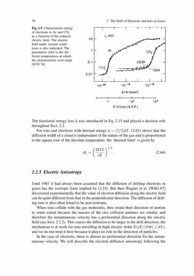
70 2 The Drift of Electrons and Ions in Gases
Fig. 2.9 Characteristic energyof electrons in Ar and CO2as a function of the reducedelectric field. The electricfield under normal condi-tions is also indicated. Theparameters refer to the dif-ferent temperatures at whichthe measurements were made[SCH 76]
The fractional energy loss λ was introduced in Eq. 2.15 and played a decisive rolethroughout Sect. 2.2.
For ions and electrons with thermal energy ε = (3/2)kT , (2.63) shows that thediffusion width of a cloud is independent of the nature of the gas and is proportionalto the square root of the absolute temperature: the ‘thermal limit’ is given by
σx =(
2kT LeE
)1/2
. (2.64)
2.2.5 Electric Anisotropy
Until 1967 it had always been assumed that the diffusion of drifting electrons ingases has the isotropic form implied by (2.55). But then Wagner et al. [WAG 67]discovered experimentally that the value of electron diffusion along the electric fieldcan be quite different from that in the perpendicular direction. The diffusion of drift-ing ions is also often found to be non-isotropic.
When ions collide with the gas molecules, they retain their direction of motionto some extent because the masses of the two collision partners are similar, andtherefore the instantaneous velocity has a preferential direction along the electricfield (see Sect. 2.2.2). This causes the diffusion to be larger in the drift direction; themechanism is at work for ions travelling in high electric fields E(eE/(Nσ) ≥ kT ),and we do not treat it here because it plays no role in the detection of particles.
In the case of electrons, there is almost no preferential direction for the instan-taneous velocity. We will describe the electron diffusion anisotropy following the
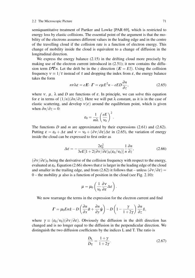
2.2 The Microscopic Picture 71
semiquantitative treatment of Partker and Lowke [PAR 69], which is restricted toenergy loss by elastic collisions. The essential point of the argument is that the mo-bility of the electrons assumes different values in the leading edge and in the centreof the travelling cloud if the collision rate is a function of electron energy. Thischange of mobility inside the cloud is equivalent to a change of diffusion in thelongitudinal direction.
We express the energy balance (2.15) in the drifting cloud more precisely bymaking use of the electron current introduced in (2.51); it now contains the diffu-sion term D∇n. Let the drift be in the z direction (E = Ez). Using the collisionfrequency ν ≡ 1/τ instead of τ and dropping the index from ε , the energy balancetakes the form
nνλε = eE ·Γ = eμE2n− eED∂n∂ z
, (2.65)
where ν , μ , λ and D are functions of ε . In principle, we can solve this equationfor ε in terms of (1/n)(∂n/∂ z). Here we will put λ constant, as it is in the case ofelastic scattering, and develop ν(ε) around the equilibrium point, which is givenwhen ∂n/∂ z = 0:
ε0 =1
mλ
(eEν0
)2
.
The functions D and m are approximated by their expressions (2.61) and (2.62).Putting ε = ε0 + Δε and ν = ν0 + (∂ν/∂ε)Δε in (2.65), the variation of energyinside the cloud can be expressed to first order as
Δε = − 2ε20
3eE[1+2(∂ν/∂ε)0(ε0/ν0)]1n
∂n∂ z
, (2.66)
(∂ν/∂ε)0 being the derivative of the collision frequency with respect to the energy,evaluated at ε0. Equation (2.66) shows that ε is larger in the leading edge of the cloudand smaller in the trailing edge, and from (2.62) it follows that – unless (∂ν/∂ε) =0 – the mobility μ also is a function of position in the cloud (see Fig. 2.10):
μ = μ0
(1ν0
∂ν∂ε
Δε)
.
We now rearrange the terms in the expression for the electron current and find
Γ = μ0Enz−D
(∂n∂x
x+∂n∂y
y
)−D
(1− γ
1+2γ
)∂n∂ z
z,
where γ ≡ (ε0/ν0)(∂ν/∂ε). Obviously the diffusion in the drift direction haschanged and is no longer equal to the diffusion in the perpendicular direction. Wedistinguish the two diffusion coefficients by the indices L and T. The ratio is
DL
DT=
1+ γ1+2γ
. (2.67)

72 2 The Drift of Electrons and Ions in Gases
Fig. 2.10 Mobility variationinside an electron cloud trav-elling in the z direction
Instead of the density distribution (2.55) of the diffusing cloud of electrons, we havein the anisotropic case
n =1√
4πDLt
(1√
4πDTt
)2
exp
[−x2 + y2
4DTt− (z−ut)2
4DLt
]. (2.68)
2.2.6 Magnetic Anisotropy
Let us now consider the effect of a magnetic field B along z. The electric field isin the x − z plane and we assume there is no electric anisotropy. The magneticfield causes the electrons to move in helices rather than in straight lines betweencollisions. Projection onto the x− y plane yields circles with radii
ρ =cω
sinθ , (2.69)
where ω = (e/m)B is the cyclotron frequency of the electron, c its velocity and θthe angle with respect to the z axis. Projection onto the x− z plane yields sinusoidalcurves. Figure 2.11a, in contrast to Fig. 2.8, shows how the random propagationof the electron is diminished by the magnetic field. We must repeat our calculation(2.60) with the new orbits.

2.2 The Microscopic Picture 73
Fig. 2.11 (a) Electron paths causing the magnetic anisotropy of diffusion. (b) First part of thetrajectory showing the direction projected into the x− y plane
Looking at Fig. 2.11b we describe the motion of the electron which has suffereda collision at the origin by the orbit
x(l) = ρ[
sin
(ωlc
−φ)
+ sinφ],
y(l) = ρ[
cos
(ωlc
−φ)− cosφ
],
z(l) = l cosθ ,
(2.70)
where l is the length of the trajectory and φ is the starting direction in the x− yplane. More precisely, the derivatives with respect to l at the origin, giving the initialdirection of the electron, are the following:
x′(0) = sinθ cosφ ,
y′(0) = sinθ sinφ ,
z′(0) = cosθ .
The mean square displacement of the electron after the first collision is givenby an integration over the solid angle and over the distribution (2.59) of pathlengths:
〈x2〉 =1
4πl0
∫e−l/l0x2(l)dφdcosθ dl (2.71)
and similarly for 〈y2〉 and 〈z2〉. It is not difficult to integrate (2.71), using (2.70) and(2.69). The result is

74 2 The Drift of Electrons and Ions in Gases
〈x2〉 = 〈y2〉 =23
l20
1+ω2l20/c
=23
l20
1+ω2τ2 ,
〈z2〉 =23
l20 .
In comparison to (2.60), the magnetic field has caused the diffusion along x and y(then perpendicular to the magnetic field) to be reduced by the factor
DT(ω)DT(0)
=1
1+ω2τ2 , (2.72)
whereas the longitudinal diffusion is the same as before:
DL(ω) = DL(0). (2.73)
If there is an E field as well as a B field in the gas, the electric and magneticanisotropies combine. In the most general case of arbitrary field directions, the diffu-sion is described by a 3×3 tensor: let the B field be along the z axis of a right-handedcoordinate system S, and let the drift direction u, which is at an angle β with respectto B, have components along z and x. The electric anisotropy is along u, and the dif-fusion tensor is diagonal in the system S′ which is rotated around y by the angle β .
In order to describe the two anisotropies in S, we must transform the diagonaltensor S′ to S before we multiply by the diagonal tensor that represents the magneticanisotropy. If the electric anisotropy is equal to DL/DT and the magnetic one isequal to D(0)/D(ω) = 1/η , we get for the combined tensor S
Dik =
⎛⎝ cosβ 0 sinβ
0 1 0−sinβ 0 cosβ
⎞⎠⎛⎝DT 0 0
0 DT 00 0 DL
⎞⎠⎛⎝ cosβ 0 −sinβ
0 1 0sinβ 0 cosβ
⎞⎠
×
⎛⎝η 0 0
0 η 00 0 1
⎞⎠ ,
Dik =
⎛⎝η(DT cos2 β +DL sin2 β ) 0 (DL −DT)sinβ cosβ
0 DT 0η(DT −DT)sinβ cosβ 0 DT sin2 β +DL cos2 β
⎞⎠ . (2.74)
The importance of diffusion for drift chambers is in the limitation for the co-ordinate measurement. Hence, we are interested in the deviation along a givendirection of an electron that has been diffusing for a time t. We treat the gen-eral case of a diffusion tensor Di j and a direction α given by the three cosineαk(α2
1 + α22 + α2
3 = 1), both expressed in the same coordinate system. We makeuse of the continuity equation (2.58) for the density n(x1,x2,x3), normalized so that∫
n dx = 1. For a time-independent and homogeneous field the drift velocity isconstant, and we have

2.2 The Microscopic Picture 75
dndt
= Dik∂ 2n
∂xi∂xk
(summation over identical indices is always understood). The rate of the meansquare deviation along x′ = αix j is given by
d〈x′2〉dt
=+∞∫
−∞
(αixi)2 dndt
dx =+∞∫
−∞
αiα jxix jDnm∂ 2n
∂xn∂xmdx = 2αiα jDi j.
In the last integral all the 81 terms vanish except when the powers of the xi matchthe powers of the derivatives: one shows by two partial integrations that
+∞∫−∞
xix j∂ 2n
∂xn∂xmdx = 2δimδ jn,
where δik = 1 if i = k, and zero otherwise. We have used the fact that electron densityand its derivatives vanish at infinity
If a point-like ensemble of electrons begins to diffuse at time zero, then after atime t it has grown so that the mean square width of the cloud in the direction α hasthe value
〈x′2〉 = 2αiα jDi jt. (2.75)
The isotropic case in which x′2 is independent of α is obviously given by a Di j
which is the unit matrix multiplied with the isotropic diffusion constant. The factor2 in (2.75) is also present in (2.55) and in the comparison between (2.60) and (2.61).Equation (2.75) implies that the width of the cloud is calculated only from the sym-metric part of Di j; furthermore, the diffusion tensor must be positive definite, other-wise our cloud would shrink in some direction–a thermo-dynamic impossibility.
2.2.7 Electron Attachment
During their drift, electrons may be absorbed in the gas by the formation of negativeions. Whereas the noble gases and most organic molecules can form only stablenegative ions at collision energies of several electronvolts (which is higher than theenergies reached during the drift in gas chambers), there are some molecules thatare capable of attaching electrons at much lower collision energies. Such moleculesare sometimes present in the chamber gas as impurities. Among all the elements,the largest electron affinities, i.e. binding energies of an electron to the atom inquestion, are found with the halogenides (3.1–3.7 eV) and with oxygen (∼0.5eV).Therefore we have in mind contaminations due to air, water, and halogen-containingchemicals.
Our account must necessarily be brief; for a thorough discussion of the atomicphysics of electron attachment, the reader is referred to Massey et al. [MAS 69].

76 2 The Drift of Electrons and Ions in Gases
Modern developments may be followed in the Proceedings of the InternationalConference on the Physics of Electronic and Atomic Collisions, see especially[CHR 81]. One distinguishes two-body and three-body processes.
The two-body process involves a molecule M that may or may not disintegrateinto various constituents A, B, . . ., one of which forms a negative ion:
e− +M → M−
ore− +M → A− +B+ . . .
The break-up of the molecule owing to the attaching electron is quite common andis called dissociative attachment. The probability of the molecule staying intact isgenerally higher at lower electron energies. The rate R of attachment is given by thecross-section σ , the electron velocity c, and the density N of the attaching molecule:
R = cσN = kN. (2.76)
The rate is proportional to the density. The constant of proportionality is calledthe two-body attachment rate-constant k.
As examples of strong attachment of slow electrons, we depict in Fig. 2.12a-d the measured cross-sections of some freons. The rate constants of many otherhalogen-containing compounds are known [MCC 81]; some of them reach several10−8 s−1 cm3 at low (thermal) electron energies.
Among the three-body processes, the Bloch–Bradbury process is the best known[BLO 35, HER 69]. It plays an important role in the absorption of electrons byoxygen molecules. At energies below 1 eV, the electron is attached to the oxygenmolecule that forms the excited and unstable state O∗−
2 . Unless the energy of excita-tion is carried away by a third body X during the lifetime of the excitation, the O∗−
2ion will lose its electron, which is then no longer attached. The lifetime τ is of theorder of 10−10 s; experimental determinations span the range between 0.02×10⁻¹⁰
and 1.0×10⁻¹⁰ s, and theoretical calculations come out between 0.88×10⁻¹⁰ and3× 10−10 s [HAT 81]. The rate R of effective attachment depends on τ , as well ason the two collision rates and the cross-sections for the two processes,
σ1 : e− +O2 → O∗−2 ,
σ2 : O∗−2 +X → O∗−
2 +X.
Let us look at a swarm of electrons in a gas that contains O2 molecules withdensity N(O2) and third bodies X with density N(X). Per electron, let the rate dn/dtof formation of the O∗−
2 state be 1/T1; if the rate of spontaneous decay is n/τ and therate of de-excitation through collision with third bodies n/T2, then the equilibriumnumber n per electron of O∗−
2 states is given by
1T1
=nτ
+nT2
,
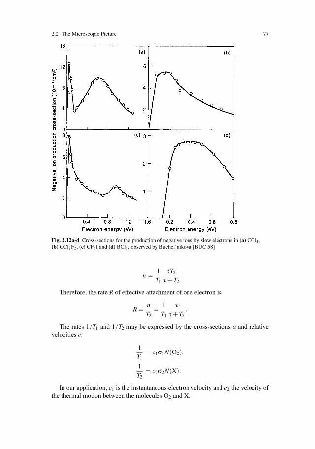
2.2 The Microscopic Picture 77
Fig. 2.12a-d Cross-sections for the production of negative ions by slow electrons in (a) CCl4,(b) CCl2F2, (c) CF3I and (d) BCl3, observed by Buchel’nikova [BUC 58]
n =1T1
τT2
τ +T2.
Therefore, the rate R of effective attachment of one electron is
R =nT2
=1T1
ττ +T2
.
The rates 1/T1 and 1/T2 may be expressed by the cross-sections a and relativevelocities c:
1T1
= c1σ1N(O2),
1T2
= c2σ2N(X).
In our application, c1 is the instantaneous electron velocity and c2 the velocity ofthe thermal motion between the molecules O2 and X.
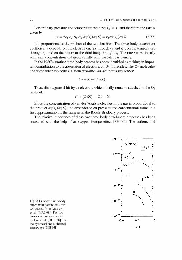
78 2 The Drift of Electrons and Ions in Gases
For ordinary pressure and temperature we have T2 � τ , and therefore the rate isgiven by
R = τc1 c2 σ1 σ2 N(O2)N(X) = k1N(O2)N(X). (2.77)
It is proportional to the product of the two densities. The three-body attachmentcoefficient k depends on the electron energy through c1 and σ1, on the temperaturethrough c2, and on the nature of the third body through σ2. The rate varies linearlywith each concentration and quadratically with the total gas density.
In the 1980’s another three-body process has been identified as making an impor-tant contribution to the absorption of electrons on O2 molecules. The O2 moleculesand some other molecules X form unstable van der Waals molecules:
O2 +X ↔ (O2X).
These disintegrate if hit by an electron, which finally remains attached to the O2
molecule:e− +(O2X) → O−
2 +X.
Since the concentration of van der Waals molecules in the gas is proportional tothe product N(O2)N(X), the dependence on pressure and concentration ratios in afirst approximation is the same as in the Bloch–Bradbury process.
The relative importance of these two three-body attachment processes has beenmeasured with the help of an oxygen-isotope effect [SHI 84]. The authors find
Fig. 2.13 Some three-bodyattachment coefficients forO2 quoted from Masseyet al. [MAS 69]. The twocrosses are measurementsby Huk et al. [HUK 88]; forthe hydrocarbons at thermalenergy, see [SHI 84]
2.3 Results from the Complete Microscopic Theory 79
examples where the van der Waal mechanism dominates, whilst the Bloch–Bradburyprocess is weak; also at higher gas pressures, the van der Waals mechanism makesa strong contribution.
For the operation of drift chambers, the absorption of electrons is a disturbingside effect that can be avoided by using clean gases. Therefore we leave out furtherrefinements that are discussed in the literature.
Some measured three-body attachment coefficients for O2 are shown in Fig. 2.13as functions of the electron energy. It can be seen that the H2O molecule is muchmore effective as the third body than the more inert atoms or the nitrogen molecule.
The three-body O2 attachment coefficient involving the methane molecule islarge enough to cause electron losses in chambers where methane is a quenchinggas. For example (compare Table 11.4), with 20% CH4 at 8.5 bar, an oxygen con-tamination of 1 ppm will cause an absorption rate of 2000/s, or roughly 3%/m ofdrift at a velocity of 6cm/μs. More information on electron attachment is collectedin Chap. 12.
2.3 Results from the Complete Microscopic Theory
In this section we quote without proof results for mobility and diffusion in theframework of the complete microscopic theory. The reader is referred to Huxleyand Crompton [HUX 74] and to Allis [ALL 56] for a more detailed discussion.
2.3.1 Distribution Function of Velocities
The principal approximation of Sect. 2.2 was to take a single velocity c to representthe motion between collisions of the drifting electrons. In reality, these velocitiesare distributed around a mean value according to a distribution function
f0(c)dc,
which represents the isotropic probability density of finding the electron in the three-dimensional velocity interval dcx dcy dcz at c. Therefore the distribution function isnormalized so that
4π∞∫
0
c2 f0(c)dc = 1.
The term ‘isotropic’ actually refers to the first, isotropic, term of an expansion inLegendre functions of the probability distribution for the vector c.
The shape of the distribution depends on the way in which the energy loss andthe cross-section vary with the collision velocity. The regime of elastic scatteringas well as a good part of the regime of inelastic scattering can be described by two
80 2 The Drift of Electrons and Ions in Gases
functions: an effective cross-section σ(c), and the fractional energy loss λ(c)(σ(c)is sometimes called the momentum transfer cross-section). Electron drift velocitiesthat are appropriate for drift chambers are achieved by electric fields that are highenough to make the random energy of the electron much higher than the thermalenergy of the gas molecules. Therefore we may neglect thermal motion. Absorptionor production of electrons (ionization) is equally excluded.
With these assumptions the distribution of the random velocities can be derived inthe framework of the Maxwell–Boltzmann transport equations [HUX 74, SCH 86,ALL 56]:
f0(c) = const exp
⎡⎣−3
ε∫0
λεdεε2
l
⎤⎦= const exp
⎡⎣ −3m
2e2E2
ε∫0
λν2dε
⎤⎦ , (2.78)
where ε = mc2/2, and εl = eEl0 = eE/(Nσ) is the energy gained through a meanfree path l0 in the direction of the field. The distribution function can also be writtenas an integral over the collision frequency ν = cNσ . The second form of (2.78)lends itself to the generalization owing to the presence of a magnetic field. For adiscussion of the range of validity of our assumptions, the reader is also referred tothe quoted literature.
In order to make a picture of such velocity distributions, we consider two limit-ing cases.
• If both the collision time τ and the fractional energy loss are independent of c,then f0(c) is the Maxwell distribution. Using (2.77) and (2.78),
f0(c) →1
(α√
π)3exp
[−( c
α
)2], (2.79)
with
α2 =4
3λ
(eEm
τ)2
.
• If both the mean free path l0 = cτ and the fractional energy loss are independentof c – an approximation that is sometimes useful in a limited range of energies –then f0(c) assumes the form of a Druyvesteyn distribution (Fig. 2.14):
f0(c) →1
α3πΓ (3/4)exp
[−( c
α
)4], (2.80)
with
α4 =8
3λ
(eEm
l0
)2
.
Once f0(c) is known, the mobility and diffusion are calculated from appropriateaverages over all velocities c.
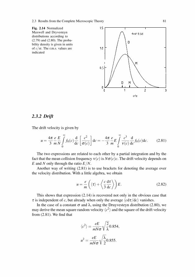
2.3 Results from the Complete Microscopic Theory 81
Fig. 2.14 NormalizedMaxwell and Dryvesteyndistributions according to(2.79) and (2.80). The proba-bility density is given in unitsof c/α . The r.m.s. values areindicated
2.3.2 Drift
The drift velocity is given by
u =4π3
em
EN
∞∫0
f0(c)ddc
[c2
σ(c)
]dc = −4π
3em
E
∞∫0
c3
ν(c)ddc
f0(c)dc. (2.81)
The two expressions are related to each other by a partial integration and by thefact that the mean collision frequency ν(c) is Nσ(c)c. The drift velocity depends onE and N only through the ratio E/N.
Another way of writing (2.81) is to use brackets for denoting the average overthe velocity distribution. With a little algebra, we obtain
u =em
(〈τ〉+
⟨c3
dτdc
⟩)E. (2.82)
This shows that expression (2.14) is recovered not only in the obvious case thatτ is independent of c, but already when only the average 〈cdτ/dc〉 vanishes.
In the case of a constant σ and λ, using the Druyvesteyn distribution (2.80), wemay derive the mean square random velocity 〈c2〉 and the square of the drift velocityfrom (2.81). We find that
〈c2〉 =eE
mNσ
√2λ
0.854,
u2 =eE
mNσ
√λ2
0.855.
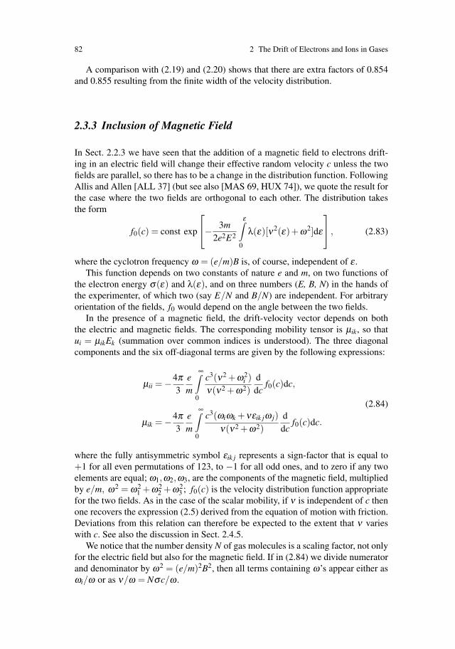
82 2 The Drift of Electrons and Ions in Gases
A comparison with (2.19) and (2.20) shows that there are extra factors of 0.854and 0.855 resulting from the finite width of the velocity distribution.
2.3.3 Inclusion of Magnetic Field
In Sect. 2.2.3 we have seen that the addition of a magnetic field to electrons drift-ing in an electric field will change their effective random velocity c unless the twofields are parallel, so there has to be a change in the distribution function. FollowingAllis and Allen [ALL 37] (but see also [MAS 69, HUX 74]), we quote the result forthe case where the two fields are orthogonal to each other. The distribution takesthe form
f0(c) = const exp
⎡⎣− 3m
2e2E2
ε∫0
λ(ε)[ν2(ε)+ω2]dε
⎤⎦ , (2.83)
where the cyclotron frequency ω = (e/m)B is, of course, independent of ε .This function depends on two constants of nature e and m, on two functions of
the electron energy σ(ε) and λ(ε), and on three numbers (E, B, N) in the hands ofthe experimenter, of which two (say E/N and B/N) are independent. For arbitraryorientation of the fields, f0 would depend on the angle between the two fields.
In the presence of a magnetic field, the drift-velocity vector depends on boththe electric and magnetic fields. The corresponding mobility tensor is μik, so thatui = μikEk (summation over common indices is understood). The three diagonalcomponents and the six off-diagonal terms are given by the following expressions:
μii = −4π3
em
∞∫0
c3(ν2 +ω2i )
ν(ν2 +ω2)ddc
f0(c)dc,
μik = −4π3
em
∞∫0
c3(ωiωk +νεik jω j)ν(ν2 +ω2)
ddc
f0(c)dc.
(2.84)
where the fully antisymmetric symbol εik j represents a sign-factor that is equal to+1 for all even permutations of 123, to −1 for all odd ones, and to zero if any twoelements are equal; ω1,ω2,ω3, are the components of the magnetic field, multipliedby e/m, ω2 = ω2
1 +ω22 +ω2
3 ; f0(c) is the velocity distribution function appropriatefor the two fields. As in the case of the scalar mobility, if ν is independent of c thenone recovers the expression (2.5) derived from the equation of motion with friction.Deviations from this relation can therefore be expected to the extent that ν varieswith c. See also the discussion in Sect. 2.4.5.
We notice that the number density N of gas molecules is a scaling factor, not onlyfor the electric field but also for the magnetic field. If in (2.84) we divide numeratorand denominator by ω2 = (e/m)2B2, then all terms containing ω’s appear either asωi/ω or as ν/ω = Nσc/ω .

2.4 Applications 83
The dependence of the drift-velocity vector on the three scalar quantities E, B,and N may therefore be written in the form
ui = μik
(EN
,BN
,φ)
Ek
N, (2.85)
where φ is the angle between the fields.This relation is important when it comes to a discussion of the gas pressure in
drift chambers (Chap. 12).
2.3.4 Diffusion
As given in the quoted literature, the isotropic diffusion coefficient is derived fromthe velocity distribution function through the integral
D = 4π∞∫
0
c2
3ν(c)f0(c)c2 dc. (2.86)
We note that expression (2.61) represented the case of one unique velocity,
4πc2 f0(c) = δ (c−〈c〉).
The magnetic anisotropy caused by a B field may be described by the 3×3 tensorDik. Its elements are given by
Dii =4π3
∞∫0
c2(ν2 +ω2i )
ν(ν2 +ω2)f0(c)c2 dc,
Dik =4π3
∞∫0
c2(ωiωk +νεik jω j)ν(ν2 +ω2)
f0(c)c2 dc.
(2.87)
For the electric anisotropy of diffusion, we must retain in the velocity distributionits dependence on position; the reader is referred to the literature [PAR 69].
2.4 Applications
In this section we discuss few practical applications of the formulae derived in theprevious sections.
2.4.1 Determination of σ(ε) and λ(ε) from Drift Measurement
In the drift of ions and electrons in gases, the quantities that are important for tracklocalization are the drift velocity and the diffusion tensor. In this chapter we have
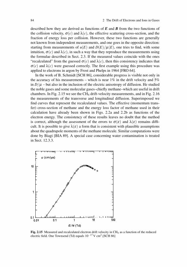
84 2 The Drift of Electrons and Ions in Gases
described how they are derived as functions of E and B from the two functions ofthe collision velocity, σ(c) and λ(c), the effective scattering cross-section, and thefraction of energy loss per collision. However, these two functions are generallynot known from independent measurements, and one goes in the opposite direction:starting from measurements of u(E) and D(E)/μ(E), one tries to find, with someintuition, σ(c) and λ(c), in such a way that they reproduce the measurements usingthe formulae described in Sect. 2.3. If the measured values coincide with the ones“recalculated” from the guessed σ(c) and λ(c), then this consistency indicates thatσ(c) and λ(c) were guessed correctly. The first example using this procedure wasapplied to electrons in argon by Frost and Phelps in 1964 [FRO 64].
In the work of B. Schmidt [SCH 86], considerable progress is visible not only inthe accuracy of his measurements – which is near 1% in the drift velocity and 5%in D/μ – but also in the inclusion of the electric anisotropy of diffusion. He studiedthe noble gases and some molecular gases–chiefly methane–which are useful in driftchambers. In Fig. 2.15 we see the CH4 drift-velocity measurements, and in Fig. 2.16the measurements of the transverse and longitudinal diffusion. Superimposed wefind curves that represent the recalculated values. The effective (momentum trans-fer) cross-section of methane and the energy loss factor of methane used in theircalculation have already been shown in Figs. 2.2a and 2.2b as functions of theelectron energy. The consistency of these results leaves no doubt that the methodis correct, although the assessment of the errors to σ(ε) and λ(ε) remains diffi-cult. It is possible to give λ(ε) a form that is consistent with plausible assumptionsabout the quadrupole moments of the methane molecule. Similar computations weredone by Biagi [BIA 89]. A special case concerning water contamination is treatedin Sect. 12.3.3.
Fig. 2.15 Measured and recalculated electron drift velocity in CH4 as a function of the reducedelectric field. One Townsend (Td) equals 10−17 V cm2.[SCH 86]

2.4 Applications 85
Fig. 2.16 Measured and recalculated transverse and longitudinal electron diffusion in CH4[SCH 86]. The ratio of the diffusion coefficients over the mobility is shown as a function of thereduced electric field
There are microwave relaxation measurements that allow an alternative deriva-tion of the cross-sections of some gases; also, there are quantum-mechanical cal-culations for the noble gases. Where a comparison of cross-sections can be made,they are identical within factors of 2 to 5, and often much better. According to thecalculations, the minimum is sharper than that derived from the drift measurementbecause the wide energy distribution smears it out. For more details, the reader isreferred to the literature.
There is a very large number of measurements of electron drift velocities anddiffusion coefficients. Many of them are collected in two compilations [FEH 83]and [PEI 84], which also contain other material that is of interest with respect todrift chambers.
Measurements in magnetic fields are rare; we present some examples inSect. 2.4.7. Precision reproductions of magnetic data, and determinations of σ(ε)and λ(ε) from them, have not yet been done.
2.4.2 Example: Argon–Methane Mixture
In this subsection we want to collect and interpret some drift and diffusion measure-ments for argon + methane mixtures without magnetic field. This gas has beeninvestigated more systematically than most others, and is being used in severallarge TPCs.
The measurements, done by Jean-Marie et al. [JEA 77], of the drift velocity asa function of the electric field E at atmospheric pressure are presented in Fig. 2.17.For all mixing ratios R there is a rising part at low E and a falling part at high E. Themaxima occur at values Ep, which depend almost linearly on the CH4 concentration,
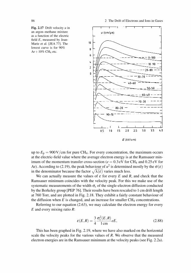
86 2 The Drift of Electrons and Ions in Gases
Fig. 2.17 Drift velocity u inan argon–methane mixtureas a function of the electricfield E, measured by Jean-Marie et al. [JEA 77]. Thelowest curve is for 90%Ar+10% CH4 etc.
up to Ep = 900V/cm for pure CH4. For every concentration, the maximum occursat the electric-field value where the average electron energy is at the Ramsauer min-imum of the momentum transfer cross-section (e = 0.3eV for CH4 and 0.25 eV forAr). According to (2.19), the peak behaviour of u2 is determined mostly by the σ(ε)in the denominator because the factor
√λ(ε) varies much less.
We can actually measure the values of ε for every E and R, and check that theRamsauer minimum coincides with the velocity peak. For this we make use of thesystematic measurements of the width σx of the single-electron diffusion conductedby the Berkeley group [PEP 76]. Their results have been rescaled to 1 cm drift lengthat 760 Torr, and are plotted in Fig. 2.18. They exhibit a fairly constant behaviour ofthe diffusion when E is changed, and an increase for smaller CH4 concentrations.
Referring to our equation (2.63), we may calculate the electron energy for everyE and every mixing ratio R:
ε(E,R) =34
σ2x (E,R)1cm
eE, (2.88)
This has been graphed in Fig. 2.19, where we have also marked on the horizontalscale the velocity peaks for the various values of R. We observe that the measuredelectron energies are in the Ramsauer minimum at the velocity peaks (see Fig. 2.2a).
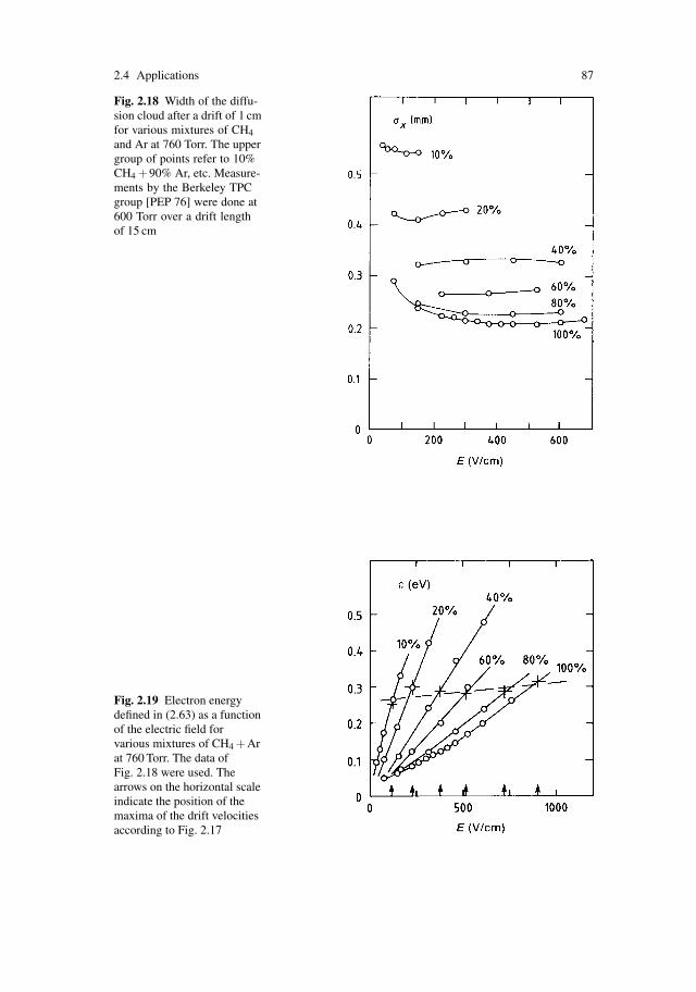
2.4 Applications 87
Fig. 2.18 Width of the diffu-sion cloud after a drift of 1 cmfor various mixtures of CH4and Ar at 760 Torr. The uppergroup of points refer to 10%CH4 +90% Ar, etc. Measure-ments by the Berkeley TPCgroup [PEP 76] were done at600 Torr over a drift lengthof 15 cm
Fig. 2.19 Electron energydefined in (2.63) as a functionof the electric field forvarious mixtures of CH4 +Arat 760 Torr. The data ofFig. 2.18 were used. Thearrows on the horizontal scaleindicate the position of themaxima of the drift velocitiesaccording to Fig. 2.17
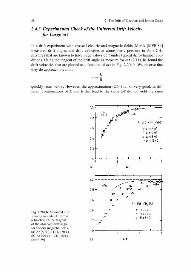
88 2 The Drift of Electrons and Ions in Gases
2.4.3 Experimental Check of the Universal Drift Velocityfor Large ωτ
In a drift experiment with crossed electric and magnetic fields, Merck [MER 89]measured drift angles and drift velocities at atmospheric pressure in Ar + CH4
mixtures that are known to have large values of τ under typical drift-chamber con-ditions. Using the tangent of the drift angle as measure for ωτ (2.11), he found thedrift velocities that are plotted as a function of ωτ in Fig. 2.20a,b. We observe thatthey do approach the limit
u → EB
quickly from below. However, the approximation (2.54) is not very good, as dif-ferent combinations of E and B that lead to the same ωτ do not yield the same
Fig. 2.20a,b Measured driftvelocity in units of E/B asa function of the tangentof the observed drift angle,for various magnetic fields.(a) Ar (50%)+ CH4 (50%),(b) Ar (95%) + CH4 (5%)[MER 89]
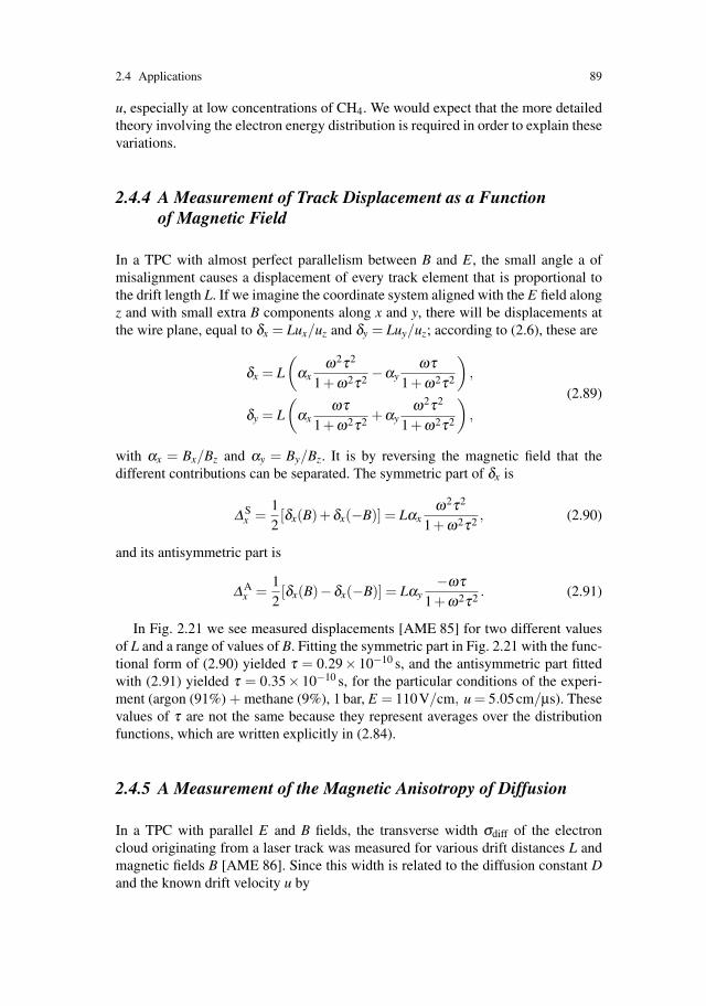
2.4 Applications 89
u, especially at low concentrations of CH4. We would expect that the more detailedtheory involving the electron energy distribution is required in order to explain thesevariations.
2.4.4 A Measurement of Track Displacement as a Functionof Magnetic Field
In a TPC with almost perfect parallelism between B and E, the small angle a ofmisalignment causes a displacement of every track element that is proportional tothe drift length L. If we imagine the coordinate system aligned with the E field alongz and with small extra B components along x and y, there will be displacements atthe wire plane, equal to δx = Lux/uz and δy = Luy/uz; according to (2.6), these are
δx = L
(αx
ω2τ2
1+ω2τ2 −αyωτ
1+ω2τ2
),
δy = L
(αx
ωτ1+ω2τ2 +αy
ω2τ2
1+ω2τ2
),
(2.89)
with αx = Bx/Bz and αy = By/Bz. It is by reversing the magnetic field that thedifferent contributions can be separated. The symmetric part of δx is
Δ Sx =
12[δx(B)+δx(−B)] = Lαx
ω2τ2
1+ω2τ2 , (2.90)
and its antisymmetric part is
Δ Ax =
12[δx(B)−δx(−B)] = Lαy
−ωτ1+ω2τ2 . (2.91)
In Fig. 2.21 we see measured displacements [AME 85] for two different valuesof L and a range of values of B. Fitting the symmetric part in Fig. 2.21 with the func-tional form of (2.90) yielded τ = 0.29× 10⁻¹⁰ s, and the antisymmetric part fittedwith (2.91) yielded τ = 0.35× 10⁻¹⁰ s, for the particular conditions of the experi-ment (argon (91%) + methane (9%), 1 bar, E = 110V/cm, u = 5.05cm/μs). Thesevalues of τ are not the same because they represent averages over the distributionfunctions, which are written explicitly in (2.84).
2.4.5 A Measurement of the Magnetic Anisotropy of Diffusion
In a TPC with parallel E and B fields, the transverse width σdiff of the electroncloud originating from a laser track was measured for various drift distances L andmagnetic fields B [AME 86]. Since this width is related to the diffusion constant Dand the known drift velocity u by

90 2 The Drift of Electrons and Ions in Gases
Fig. 2.21 Measured track displacements due to a small angle between the electric and magneticfields; (a) symmetric part, (b) antisymmetric part. The curves are fits to (2.90) and (2.91). CurvesA: L = 126cm; curves B: L = 65cm [AME 85]
σ2diff(L,B) = 2D(B)L/u,
we determined D(B). The quantity actually observed, σ21 , was the quadratic sum of
σdiff and of a constant, σ0, given by the width of the laser beam and the electrodeconfiguration. Figure 2.22 depicts the observations.
If we express the factor D(0)/D(B) by which the magnetic field reduces thediffusion constant as a function of B2, we see a linear behaviour for small B2 as well
Fig. 2.22 Measured dependence of σ21 on the magnetic field and the drift length. The slope
decreases with increasing B as the diffusion is reduced [AME 86]

2.4 Applications 91
Fig. 2.23 The factor by whichthe magnetic field reduces thetransverse diffusion in theexample elaborated in thetext. It is a linear function ofB2 for both small and large B[AME 86]
as for large B2. The transition region between the two straight lines is around 6kG2
(see Fig. 2.23). The interpretation is the following.Referring to (2.84) and (2.87) we note that the off-diagonal elements of the dif-
fusion tensor do not contribute to σdiff. We write
D11(ω) =4π3
∞∫0
c2νν2 +ω2 f0(c)c2dc =
⟨c2ν
3(ν2 +ω2)
⟩.
This expression can be evaluated in the two limiting cases of ω2 small and ω2
large compared with ν20 , the square of a typical collision frequency ν0. For this
typical frequency we may take the value derived from the electron mobility μ in thelimit in which ν is independent of c : ν0 = (e/m)/μ . We find in lowest order
D11(0)D11(B)
= 1+ω2τ21 , ω2 ν2
0 ,
D11(0)D11(B)
= C +ω2τ22 , ω2 ν2
0 .
(2.92)
The values of
τ21 =
〈c2/ν3〉〈c2/ν〉 ,
τ22 =
〈c2/ν〉〈c2/ν〉 ,
C =〈c2/ν〉〈c2ν3〉
〈c2ν〉2 (2.93)
are independent of ω , because the two fields are parallel to each other.Since ν is a function of c and is therefore distributed over a wide range of
values, the averages in (2.93) are all different. In fact the straight lines in Fig. 2.23
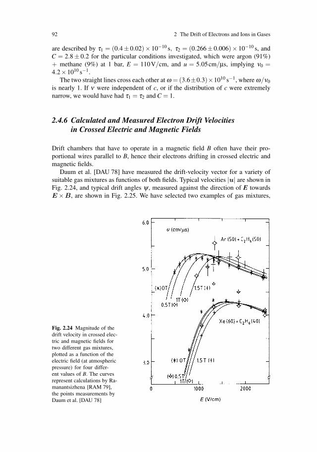
92 2 The Drift of Electrons and Ions in Gases
are described by τ1 = (0.4± 0.02)× 10−10 s, τ2 = (0.266± 0.006)× 10−10 s, andC = 2.8± 0.2 for the particular conditions investigated, which were argon (91%)+ methane (9%) at 1 bar, E = 110V/cm, and u = 5.05cm/μs, implying ν0 =4.2×10¹⁰ s−1.
The two straight lines cross each other at ω = (3.6±0.3)×1010 s−1, where ω/ν0
is nearly 1. If ν were independent of c, or if the distribution of c were extremelynarrow, we would have had τ1 = τ2 and C = 1.
2.4.6 Calculated and Measured Electron Drift Velocitiesin Crossed Electric and Magnetic Fields
Drift chambers that have to operate in a magnetic field B often have their pro-portional wires parallel to B, hence their electrons drifting in crossed electric andmagnetic fields.
Daum et al. [DAU 78] have measured the drift-velocity vector for a variety ofsuitable gas mixtures as functions of both fields. Typical velocities |u| are shown inFig. 2.24, and typical drift angles ψ , measured against the direction of E towardsE ×B, are shown in Fig. 2.25. We have selected two examples of gas mixtures,
Fig. 2.24 Magnitude of thedrift velocity in crossed elec-tric and magnetic fields fortwo different gas mixtures,plotted as a function of theelectric field (at atmosphericpressure) for four differ-ent values of B. The curvesrepresent calculations by Ra-manantsizhena [RAM 79],the points measurements byDaum et al. [DAU 78]
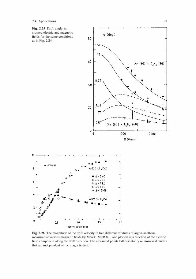
2.4 Applications 93
Fig. 2.25 Drift angle incrossed electric and magneticfields for the same conditionsas in Fig. 2.24
Fig. 2.26 The magnitude of the drift velocity in two different mixtures of argon–methane,measured at various magnetic fields by Merck [MER 89], and plotted as a function of the electricfield component along the drift direction. The measured points fall essentially on universal curvesthat are independent of the magnetic field

94 2 The Drift of Electrons and Ions in Gases
argon + ethane, and xenon + ethane, which exhibit different mobilities and,therefore, different values of ωτ at a given magnetic field.
These measurements have been compared with calculations based on the for-malism explained in Sect. 2.3, by Ramanantsizhena [RAM 79]. He used elasticcross-sections for the e−C2H6 collision, which are based on the work of Duncan andWalker [DUN 74], and inelastic cross-sections derived from Palladino and Sadoulet[PAL 75]. Comparing the measurements with the calculations, we notice that agree-ment exists, mostly at the level of 5 to 10%, occasionally worse. In addition weobserve the small variation of the calculated maximum of the drift velocity as themagnetic field is changed: according to Tonks’ theorem it should stay the same, butwith a realistic distribution function it decreases by 1 or 2% for the gas mixtures ofFig. 2.24 as B goes up from 0 to 1.5 T.
In Fig. 2.26 we see drift velocities measured by Merck [MER 89] in crossedelectric and magnetic fields as functions of the electric field component along thedrift direction. We note that the points belonging to different B fall on the sameline characteristic of the gas, within the measurement error, which is 2 or 3% (onlyfor the small CH4 concentration is there a 12% deviation near the peak). ObviouslyTonks’ theorem, (2.13) and (2.51), is quite well confirmed.
References
[ALL 31] W.P. Allis and P.M. Morse, Theorie der Streuung langsamer Elektronen an Atomen,Z. Phys. 70, 567 (1931)
[ALL 37] W.P. Allis and H.W. Allen, Theory of the Townsend method of measuring electrondiffusion and mobility, Phys. Rev. 52, 703 (1937)
[ALL 56] W.P. Allis, Motions of ions and electrons, in Handbuch der Physik, vol. XXI, ed. byS. Flugge, (Springer, Berlin Heidelberg, 1956), p. 383
[AME 85] S.R. Amendolia et al., Calibration of field inhomogeneities in a time projection cham-ber with laser rays, Nucl. Instrum. Methods Phys. Res. A235, 296 (1985)
[AME 86] S.R. Amendolia et al., Dependence of the transverse diffusion of drifting electrons onmagnetic field, Nucl. Instrum. Methods Phys. Res. A244, 516 (1986)
[ATR 77] V.M. Atrazhev and I.T. Iakubov, The electron drift velocity in dense gases, J. Phys.D10, 2155 (1977)
[BIA 89] S.F. Biagi, A multiform Boltzmann analysis of drift velocity, diffusion, gain andmagnetic effects in argon–methane–water-vapour mixtures, Nucl. Instr. Meth. A283,716 (1989)
[BLO 35] F. Bloch and N.E. Bradbury, On the mechanism of unimolecular electron capture,Phys. Rev. 48, 689 (1935)
[BRA 81] G.L. Braglia and V. Dallacasa, Multiple scattering theory of electron mobility in densegases, in [CHR 81], p. 83
[BRO 66] S.C. Brown, Introduction to Electrical Discharges in Gases (Wiley, New York 1966)[BUC 58] I.S. Buchel’nikova, Cross sections for the capture of slow electrons by O2 and H2O
molecules and molecules of halogen compounds, Zh. Eksper. Teor. Fiz. 35, 1119(1958); Sov. Phys.-JETP 35 (8), 783 (1959)
[CHR 71] L.G. Christophorou, Atomic and Molecular Radiation Physics (Wiley, London 1971)[CHR 81] L.G. Christophorou (ed.), Proc. Second International Swarm Seminar, Oak Ridge,
USA, 1981 (Pergamon, New York 1981)

References 95
[DAU 78] H. Daum et al., Measurements of electron drift velocities as a function of electric andmagnetic fields in several gas mixtures, Nucl. Instrum. Methods 152, 541 (1978)
[DUN 74] C.W. Duncan and I.C. Walker, Collision cross-sections for low-energy electrons insome simple hydro-carbons, J. Chem. Soc. Faraday Trans. II.70, 577 (1974)
[DYD 04] The authors thank F. Dydak who pointed out that the first edition of the book wasunclear about this and contained an error.
[FEH 83] J. Fehlmann and G. Viertel, Compilation of data for drift chamber operation, IHPDetector Group Note, ETH Zurich, 1983, unpublished
[FRO 64] L.S. Frost and A.V. Phelps, Momentum transfer cross-sections for slow electrons inHe, Ar, Kr and Xe from transport coefficients, Phys. Rev. A 136, 1538 (1964)
[HAT 81] Y. Hatano and H. Shimamori, Electron attachment in dense gases, in [CHR 81], p. 103[HER 69] A. Herzenberg, Attachment of flow electrons to oxygen molecules, J. Chem. Phys. 51,
4942 (1969)[HUK 88] M. Huk, P. Igo-Kemenes and A. Wagner, Electron attachment to oxygen, water, and
methanol, in various drift chamber gas mixtures, Nucl. Instrum. Methods Phys. Res.A 267, 107 (1988)
[HUX 74] L.G.H. Huxley and R.W. Crompton, The diffusion and drift of electrons in gases(Wiley, New York 1974)
[JEA 77] B. Jean-Marie, V. Lepeltier and D. L’Hote, Systematic measurement of elec-tron drift velocity and study of some properties of four gas mixtures:Ar-CH4, Ar-C2H4, Ar-C2H6, Ar-C3H8, Nucl. Instrum. Methods 159, 213 (1979)
[LAN 57] Landolt-Bornstein, vol. IV/3, Eigenschaften des Plasmas, no. 44315, 6th edn.(Springer, Berlin Heidelberg 1957)
[MAS 69] H.S.W. Massey, E.H.S. Burhop and H.B. Gilbody, Electronic and Ionic Impact Phe-nomena, 2nd edn. (Clarendon, Oxford 1969), 4 vols.
[MCC 81] D.L. McCorkle, L.G. Christophorou and S.R. Hunter, Electron attachment rate con-stants and cross-sections for halocarbons, in [CHR 81], p. 21
[MCD 73] E.W. McDaniel and E.A. Mason, The Mobility and Diffusion of Ions in Gases (Wiley,New York 1973)
[MER 89] M. Merck, Messung des Driftgeschwindigkeitsvektors von Elektronen in Gasen imgekreuzten elektrischen und magnetischen Feld, Diploma Thesis, Munich University,1989, unpublished
[PAL 75] V. Palladino and B. Sadoulet, Application of classical theory of electrons in gases todrift proportional chambers, Nucl. Instrum. Methods 128, 323 (1975)
[PAR 69] J.H. Parker, Jr. and J.J. Lowke, Theory of electron diffusion parallel to electric fields,Phys. Rev. 181 (1969): I–Theory, p. 290; II–Application to real gases, p. 302
[PEI 84] A. Peisert and F. Sauli, Drift and diffusion of electrons in gases: a compilation, CERNreport 84–08 (1984)
[PEP 76] Johns Hopkins University, LBL, UC Riverside, and Yale University (PEP Expt. No.4), Proposal for a PEP facility based on the time projection chamber (TPC), Stanfordreport SLAC-Pub-5012 (1976)
[RAM 21] C. Ramsauer, Uber den Wirkungsquerschnitt der Gasmolekule gegenuber langsamenElektronen, Ann. Phys. 66, 546 (1921)
[RAM 79] P. Ramanantsizhena, Vitesse de migration des electrons et autres coefficients detransport dans les melanges argon-ethane et xenon-ethane. Influence d’une inductionmagnetique, These, Univ. Louis-Pasteur, Strasbourg, 1979, unpublished
[SCH 76] G. Schultz, Etude d’un detecteur de particules a tres haute precision spatiale (chambrea drift), These, Univ. Louis-Pasteur, Strasbourg, 1976, unpublished
[SCH 77] G. Schultz, G. Charpak and F. Sauli, Mobilities of positive ions in some gas mixturesused in proportional and drift chambers, Rev. Phys. Appl. (France) 12, 67 (1977)
[SCH 86] B. Schmidt, Drift and Diffusion von Elektronen in Methan and Methan-Edelgas-Mischungen, Dissertation, Univ. Heidelberg, 1986, unpublished
[SHI 84] H. Shimamori and H. Hotta, Mechanism of thermal electron attachment to O2 isotopeeffect studied with 18O2 in rare gases and some hydrocarbons, J. Chem. Phys. 81,1271 (1984))

96 2 The Drift of Electrons and Ions in Gases
[TON 55] L. Tonks, Particle transport, electric currents and pressure balance in a magneticallyimmobilized plasma, Phys. Rev. 97, 1443 (1955)
[WAG 67] E.B. Wagner, F.J. Davies and G.S. Hurst, Time-of-flight investigations of electrontransport in some atomic and molecular gases. J. Chem. Phys. 47, 3138 (1967)
Chapter 3Electrostatics of Tubes, Wire Gridsand Field Cages
The electric field in a drift chamber must provide two functions: drift and amplifi-cation. Whereas in the immediate vicinity of the thin proportional or ‘sense’ wirethe cylindrical electric field provides directly the large field strengths required forcharge amplification, the drift field must be created by a suitable arrangement ofelectrodes that are set at potentials supplied by external voltage sources. It is truethat drift fields have also been created by depositing electric charges on insulators –such chambers are described in Sect. 11.4 – but we do not treat them here. Chargeamplification is not necessarily confined to proportional wires. It has also been mea-sured between parallel plates and between a wire mesh and a metal plate as well asin the tiny holes in a plate coated on both sides with the metal layers of a condenser.In fact these MICROMEGA and GEM counters seem to have a promising future[FAB 04].
There is a large variety of drift chambers, and they have all different electrodearrangements. An overview of existing chambers is given in Chap. 11, where wedistinguish three basic types. In the volume-sensitive chambers (types 2 and 3) thefunctions of drift and amplification are often more or less well separated, either byspecial wire grids that separate the drift space from the sense wire or at least bythe introduction of ‘field’ or ‘potential’ wires between the sense wires. The driftfield, which fills a space large compared to the amplification space, then has to bedefined at its boundaries; these make up the ‘field cage’. For a uniform field, theelectrodes at the boundaries are at graded potentials in the field direction and atconstant potentials orthogonal to it.
Also the area-sensitive chambers (type 1) have often been built with ‘potential’or ‘field-shaping’ wires to provide a better definition and a separate adjustment ofthe drift field. In this chapter we want to discuss some elements that are typical forthe volume-sensitive chambers with separated drift and amplification spaces: one orseveral grids with regularly spaced wires in conjunction with a field cage. Althoughdirectly applicable to a time projection chamber (TPC), the following considerationswill also apply to many type 2 chambers.
Electrostatic problems of the most general electrode configuration are usuallysolved by numerical methods, for example using relaxation techniques [WEN 58].
W. Blum et al., Particle Detection with Drift Chambers, 97doi: 10.1007/978-3-540-76684-1 3, c© Springer-Verlag Berlin Heidelberg 2008
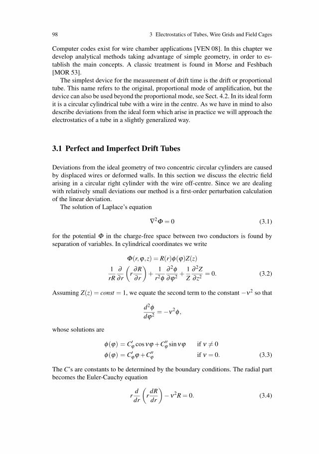
98 3 Electrostatics of Tubes, Wire Grids and Field Cages
Computer codes exist for wire chamber applications [VEN 08]. In this chapter wedevelop analytical methods taking advantage of simple geometry, in order to es-tablish the main concepts. A classic treatment is found in Morse and Feshbach[MOR 53].
The simplest device for the measurement of drift time is the drift or proportionaltube. This name refers to the original, proportional mode of amplification, but thedevice can also be used beyond the proportional mode, see Sect. 4.2. In its ideal formit is a circular cylindrical tube with a wire in the centre. As we have in mind to alsodescribe deviations from the ideal form which arise in practice we will approach theelectrostatics of a tube in a slightly generalized way.
3.1 Perfect and Imperfect Drift Tubes
Deviations from the ideal geometry of two concentric circular cylinders are causedby displaced wires or deformed walls. In this section we discuss the electric fieldarising in a circular right cylinder with the wire off-centre. Since we are dealingwith relatively small deviations our method is a first-order perturbation calculationof the linear deviation.
The solution of Laplace’s equation
∇2Φ = 0 (3.1)
for the potential Φ in the charge-free space between two conductors is found byseparation of variables. In cylindrical coordinates we write
Φ(r,ϕ,z) = R(r)φ(ϕ)Z(z)
1rR
∂∂ r
(r
∂R∂ r
)+
1r2φ
∂ 2φ∂ϕ2 +
1Z
∂ 2Z∂ z2 = 0. (3.2)
Assuming Z(z) = const = 1, we equate the second term to the constant −ν2 so that
d2φdϕ2 = −ν2φ ,
whose solutions are
φ(ϕ) = C′ϕ cosνϕ +C′′
ϕ sinνϕ if ν �= 0
φ(ϕ) = C′ϕ ϕ +C′′
ϕ if ν = 0. (3.3)
The C’s are constants to be determined by the boundary conditions. The radial partbecomes the Euler-Cauchy equation
rddr
(r
dRdr
)−ν2R = 0. (3.4)

3.1 Perfect and Imperfect Drift Tubes 99
If ν = 0, the solution is given by
R(r) = C′r lnr +C′′
r . (3.5)
3.1.1 Perfect Drift Tube
The potential between two coaxial cylinders is a straight application of Eq. (3.5).When the outer cylinder (radius b) is on ground, and the wire (radius a) on positivepotential U , one determines the coefficients to be given by C′
ϕ = 0, C′′r = −C′
r lnband C′
rC′′ϕ ln(a/b) = U , so that
Φ =U
ln(a/b)ln(
rb). (3.6)
The electric field is directed radially outwards, and
Er = −∂Φ∂ r
=U
ln(b/a)1r. (3.7)
Another way to calculate Er is using Gauss’ theorem according to which
Er =λ
2πε0
1r
(3.8)
where λ is the linear charge density on the wire; the value of ε0 is 8.854 · 10−12
As/Vm. Therefore the capacitance per unit length of tube is given by
C =λU
=2πε0
ln(b/a).
3.1.2 Displaced Wire
Solution of the Electrostatic Problem
Let the wire be displaced from the tube centre by the distance d in the negative y-direction (Fig. 3.1). The wire defines the centre of the coordinate system so that thefirst boundary condition is
Φ(a) = U, independent of ϕ . (3.9)
We must express the second boundary by the radius vector as a function of ϕ . Theexact expression is
ρ = d sinϕ +b√
(1− (d2/b2)(1− sin2 ϕ),

100 3 Electrostatics of Tubes, Wire Grids and Field Cages
Fig. 3.1 Geometry ofdisplaced wire
but we are only interested in small wire displacements. To first order in d/b we havethe boundary at
ρ = b+d sinϕ, (3.10)
and the second boundary condition is
Φ(ρ) = 0. (3.11)
Now we must determine the various coefficients using (3.9) and (3.11). To the firstorder in d/b we have solutions for ν = 0 and ν = 1, and the most general solution is
Φ = (C0′r lnr +C0′′
r )C0′′ϕ +(C1′
r r +C1′′r /r)(C1′
ϕ cosϕ +C1′′ϕ sinϕ). (3.12)
Inserting (3.9), we have to require
C1′r a+C1′′
r /a = 0, (3.13)
which implies that C1′′r can be neglected against C1′
r for the entire space except inthe immediate vicinity of the wire surface.
When inserting (3.11) and (3.10) into (3.12) we make use of the relation
ln(b+d sinϕ) = lnb+(d/b)sinϕ,
which holds to first order in d/b. This determines the constants C0′r , C0′′
r and C0′′ϕ as
in the case (3.6) of the perfect tube. Comparing factors that multiply the sinϕ-terms,we find
C0′′ϕ C0′
r (d/b)+C1′r bC1′′
ϕ = 0
or
C1′r C1′′
ϕ = − db2
Uln(a/b)
(3.14)
whereas C1′ϕ = 0. This produces the solution, in first order of (d/b), equal to
Φ(r,ϕ) =U
ln(a/b)ln
rb− U
ln(a/b)db
rb
sinϕ. (3.15)

3.1 Perfect and Imperfect Drift Tubes 101
The perturbing potential Φ1 caused by the wire displacement is given by thesecond term. Using y = r sinϕ , the field perturbation is calculated to be
(E1)y = −∂Φ1
∂y= − U
ln(b/a)db2 (3.16)
(E1)x = (E1)z = 0. (3.17)
It describes a constant field directed towards negative y, whose magnitude is d/btimes the value of the unperturbed field (3.7) at the wall.
For the purpose of calculating the electrostatic force on the wire (see furtherdown) we also record the value of (E1)y on the wire surface (r = a). Startingfrom (3.13) without the previous simplification C1′′
r = 0, the correct perturbationpotential is
Φ1(r,ϕ) =−U
ln(a/b)db2 (r− a2
r)sinϕ. (3.18)
The field in y-direction equals
(E1(a))y = −∂Φ1
∂yevaluated at r = a
= − Uln(b/a)
2db2 sin2 ϕ
Averaging over ϕ we have an extra field on the wire surface equal to
(E1(a))y = − Uln(b/a)
db2 (3.19)
The average extra field on the wire surface is as large as the field perturbation (3.16),(3.17) throughout the volume.
Gravitational Sag
The main reason for wire displacement is the weight of the wire. Even when strungwith a pulling force T close to the breaking limit, wires in several metre long tubeswill experience a gravitational sag that is large in comparison with the achievableaccuracy of drift tubes.
In order to derive a formula for the amount of bowing we introduce the coordi-nates y (downwards) and x (horizontal). We note that on every length element dx theweight of the wire is
ρgσ dx (3.20)
(ρ = density, σ = cross sectional area of the wire, g = 981cm/s2). It must be com-pensated by the vertical component of the tension at this point, which is equal to thedifference of the slopes at the two ends of the interval dx, multiplied by the pullingforce T :
−T [y′(x+dx)− y′(x)] (3.21)

102 3 Electrostatics of Tubes, Wire Grids and Field Cages
where the primes denote the first derivative. In this approximation we have assumedthat the pulling force is the same for all x, the variation due to the weight of the wirebeing negligible for practical tubes.
Combining (3.20) and (3.21), one has the differential equation
−y′′ = C = ρgσ/T (3.22)
with the solutiony = (C/2)x2 +C1x+C2. (3.23)
Specifying that y = 0 at x = ±L/2 determines the coefficients C1, C2, and the solu-tion becomes
y =C2
(L2
4− x2
). (3.24)
The point of the maximum excursion is the sagitta, equal to
s = y(0) =CL2
8=
ρgσL2
8T. (3.25)
It is proportional to the inverse of the mechanical tension. If the tension is in-creased the sagitta is reduced, but the tension cannot be arbitrarily increased sincenon-elastic deformations take place. The maximum pulling force Tc that can beapplied to a wire is proportional to its cross section, and the ratio Tc/σ is con-stant (except for very thin wires). The minimum achievable sagitta of a wire ofgiven length is independent of the wire cross section. The values of the critical ten-sion and typical sagittas for 100-cm-long wires of different materials are shown inTable 3.1. Usually the wires are strung to a tension close to the critical one in or-der to reduce the sagging. Inspecting Table 3.1 we notice that among the variousmaterials, tungsten is the one that allows the smallest sagittas but at the expenseof quite a large tension, for a given diameter of the wire. Since the tension of thewires is held by the endplates of the chamber, a large tension requires stiff end-plates. In the design of a chamber one usually compromises between these twoparameters.
If the sagitta of long wires cannot be constructed to be small one may be obligedto control its size within small tolerances. A practical way of doing this is by mea-suring the oscillation frequency of the wire. The frequency f1 of the lowest mode ofthe elastic string is
Table 3.1 Maximum stresses before deformation of typical wire materials and correspondingsagittas for 1-m-long wires
Material Tc/σ (kg/mm2) Sagitta (μm) of a 100 cm long wirestrung at Tc
Al 4 . . .16 21 . . .84Cu 21 . . .37 30 . . .53Fe 18 . . .25 39 . . .54W 180 . . .410 6 . . .13

3.1 Perfect and Imperfect Drift Tubes 103
f1 =1
2L
√T
ρσ. (3.26)
Inserting (3.25) into (3.26) produces the simple relation
f 21 =
g32s
. (3.27)
Electrostatic Force on the Sagged Wire
The displacement of the wire creates an average field (3.19) which acts on theelectric charge of the wire and produces a force which tends to increase the dis-placement. The differential equation (3.22) needs to be complemented by a termwhich represents the electrostatic force per unit wire length. This is given by theproduct
λ · (E1(a))y
where λ is given by (3.8) in terms of the unperturbed field, and (E1(a))y is given by(3.19) and is proportional to the displacement y. The electrostatic force, like grav-ity, points downwards and leads to a positive term on the right-hand side of (3.22),whereas y′′ < 0. Therefore, the differential equation is
y′′ + k2y+C = 0 (3.28)
with C = ρgσ/T and k2 = 2πε0E20 (b)/T . The value of k is plotted against E0(b)
and T in Fig. 3.2.The general solution of (3.28) is
y = C1 cos kx+C2 sin kx−C/k2. (3.29)
When specifying y(±L/2) = 0, the coefficients C1, C2 are determined, and the so-lution becomes
y =Ck2
(1
cos(kL/2)cos kx−1
). (3.30)
The electrostatic force has changed the form of the wire from the parabola (3.24) tothe cosine function (3.30).
The new sagitta is
sk = y(0) =Ck2
(1
cos(kL/2)−1
)kL1−→ CL2
8(3.31)
This means the electrostatic force has increased the sagitta (3.25) by the factor
sk
s=
8k2L2
(1
cos(kL/2)−1
)=
2q2
(1
cos q−1
). (3.32)
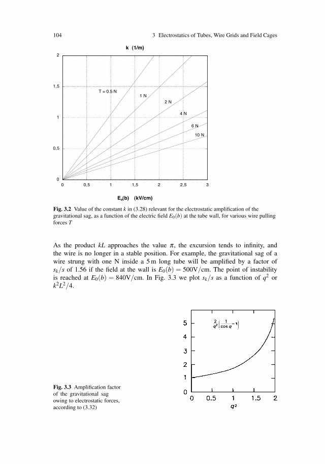
104 3 Electrostatics of Tubes, Wire Grids and Field Cages
Fig. 3.2 Value of the constant k in (3.28) relevant for the electrostatic amplification of thegravitational sag, as a function of the electric field E0(b) at the tube wall, for various wire pullingforces T
As the product kL approaches the value π , the excursion tends to infinity, andthe wire is no longer in a stable position. For example, the gravitational sag of awire strung with one N inside a 5 m long tube will be amplified by a factor ofsk/s of 1.56 if the field at the wall is E0(b) = 500V/cm. The point of instabilityis reached at E0(b) = 840V/cm. In Fig. 3.3 we plot sk/s as a function of q2 ork2L2/4.
Fig. 3.3 Amplification factorof the gravitational sagowing to electrostatic forces,according to (3.32)

3.2 Wire Grids 105
3.2 Wire Grids
3.2.1 The Electric Field of an Ideal Grid of Wires Parallelto a Conducting Plane
We assume a reference system with the x− y plane coincident with the conductingplane (pad plane) and the y axis along the direction of the wires of the grid. The zaxis is perpendicular to the plane (see Fig. 3.4).
The potential is a function of the coordinates x and z only, because the problemhas a translational symmetry along the y direction. We assume the zero of the po-tential on the conducting plane (z = 0). The complex potential of a single line ofcharge λ per unit length placed at U ′ = x′ + iz′ is
φ(U) = − λ2πε0
ln(U −U ′)(U −U ′)
, (3.33)
where U = x+ iz is the coordinate of a general point and U ′ = x′ − iz′ is the complexconjugate of U ′. MKS units are used throughout.
The potential of the whole grid is obtained by adding up the contributions ofeach wire:
φ(U) = − λ2πε0
k=+∞
∑k=−∞
ln(U −U ′
k)(U −U ′
k),
where U ′k is the coordinate of the kth wire.
All the wires of the grid are equispaced with a pitch s: therefore
U ′k = x0 + ks+ iz0(k = . . .−2,−1,0,1,2, . . .),
where x0 and z0 are the coordinates of the 0th wire of the grid. The potential of thegrid can be written as
φ(U) = − λ2πε0
k=+∞
∑k=−∞
ln(U −U ′
0 − ks)(U −U ′
0 − ks).
This summation can be computed [ABR 65]:
Fig. 3.4 An ideal grid ofwires parallel to a conductingplane

106 3 Electrostatics of Tubes, Wire Grids and Field Cages
φ(U) = − λ2πε0
lnsin[(π/s)(U −U ′
0)]sin[(π/s)(U −U ′
0)]
and the corresponding real potential is
V (x,z) = Re φ(U)
= − λ4πε0
lnsin2[(π/s)(x− x0)]+ sin h2[(π/s)(z− z0)]sin2[(π/s)(x− x0)]+ sin h2[(π/s)(z+ z0)]
. (3.34)
Figure 3.5a shows V (x, z) as function of z at two different values of x. In the chosenexample the grid was placed at z0 = s. We notice that such a grid behaves almosteverywhere like a simple layer of charge with surface density λ/s. Only in the imme-diate vicinity of the wires (distances much smaller than the pitch) can the structureof the grid be seen (compare with Fig. 3.5b, which shows the potential of a simplelayer of charge). Therefore it is possible to superimpose different grids or plane elec-trodes at distances larger than the pitch without changing the boundary conditionsof the electrostatic problem. We have an example of the general two-dimensionalproblem where a potential φ that varies periodically in one direction x has everyFourier component ≈ cos(2πnx/s) damped along the transverse direction z accord-ing to the factor e−2πnz/s. This holds because every Fourier component must satisfyLaplace’s equation
∂ 2φ∂x2 +
∂ 2φ∂ z2 = 0
Fig. 3.5 (a) The potential V (x,z) of a grid of wires situated a distance z0 from a conducting planeat x0, x0 + s, . . . with pitch s = z0 and a linear charge density λ per wire. (b) The potential V (z) ofa plane of charge situated a distance z0 from a conducting plane, with a surface charge density σ
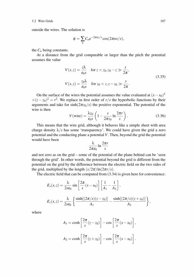
3.2 Wire Grids 107
outside the wires. The solution is
φ = ∑n
Cne−2πnz/s cos(2πnx/s),
the Cn being constants.At a distance from the grid comparable or larger than the pitch the potential
assumes the value
V (x,z) =zλε0s
for z < z0,z0 − z � s2π
,
V (x,z) =z0λε0s
for z0 < z,z− z0 �s
2π.
(3.35)
On the surface of the wires the potential assumes the value evaluated at (x− x0)2
+(z− z0)2 = r2. We replace in first order of r/s the hyperbolic functions by theirarguments and take for sinh(2πz0/s) the positive exponential. The potential of thewire is then
V (wire) =λz0
ε0s
(1− s
2πz0ln
2πrs
). (3.36)
This means that the wire grid, although it behaves like a simple sheet with areacharge density λ/s has some ‘transparency’. We could have given the grid a zeropotential and the conducting plane a potential V . Then, beyond the grid the potentialwould have been
λ2πε0
ln2πr
s
and not zero as on the grid – some of the potential of the plane behind can be ‘seenthrough the grid’. In other words, the potential beyond the grid is different from thepotential on the grid by the difference between the electric field on the two sides ofthe grid, multiplied by the length (s/2π) ln(2πr/s).
The electric field that can be computed from (3.34) is given here for convenience:
Ex(x,z) =λ
2sε0sin
[2πs
(x− x0)][
1A1
− 1A2
],
Ez(x,z) =λ
2sε0
{sinh[(2π/s)(z− z0)]
A1− sinh[(2π/s)(z+ z0)]
A2
},
where
A1 = cosh
[2πs
(z− z0)]− cos
[2πs
(x− x0)],
A2 = cosh
[2πs
(z+ z0)]− cos
[2πs
(x− x0)].
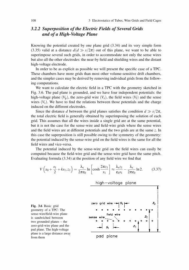
108 3 Electrostatics of Tubes, Wire Grids and Field Cages
3.2.2 Superposition of the Electric Fields of Several Gridsand of a High-Voltage Plane
Knowing the potential created by one plane grid (3.34) and its very simple form(3.35) valid at a distance d(d � s/2π) out of this plane, we want to be able tosuperimpose several such grids, in order to accommodate not only the sense wiresbut also all the other electrodes: the near-by field and shielding wires and the distanthigh-voltage electrode.
In order to be as explicit as possible we will present the specific case of a TPC.These chambers have more grids than most other volume-sensitive drift chambers,and the simpler cases may be derived by removing individual grids from the follow-ing computations.
We want to calculate the electric field in a TPC with the geometry sketched inFig. 3.6. The pad plane is grounded, and we have four independent potentials: thehigh-voltage plane (Vp), the zero-grid wire (Vz), the field wires (Vf) and the sensewires (Vs). We have to find the relations between those potentials and the chargeinduced on the different electrodes.
Since the distance d between the grid planes satisfies the condition d � s/2π ,the total electric field is generally obtained by superimposing the solution of eachgrid. This assumes that all the wires inside a single grid are at the same potential,but it is not the case for the sense-wire and field-wire grids where the sense wiresand the field wires are at different potentials and the two grids are at the same z. Inthis case the superposition is still possible owing to the symmetry of the geometry:the potential induced by the sense-wire grid on the field wires is the same for all thefield wires and vice-versa.
The potential induced by the sense-wire grid on the field wires can easily becomputed because the field-wire grid and the sense-wire grid have the same pitch.Evaluating formula (3.34) at the position of any field wire we find that
V(
x0 +s1
2+ ks1,z1
)=
λs
2πε0ln
[cosh
2πz1
s1
]≈ λsz1
ε0s1− λs
2πε0ln2. (3.37)
Fig. 3.6 Basic gridgeometry of a TPC: Thesense-wire/field-wire planeis sandwiched betweentwo grounded planes – thezero-grid-wire plane and thepad plane. The high-voltageplane is a large distance awayfrom them

3.2 Wire Grids 109
We can now use (3.35), (3.36) and (3.37) to calculate the potential of each elec-trode as the sum of the contributions of the charges induced on each grid and on thehigh-voltage plane:
Vs =λsz1
ε0s1
(1− s1
2πz1ln
2πrs
s1
)+
λfz1
ε0s1
(1− s1
2πz1ln2
)+
λzz1
s2ε0+
σpz1
ε0,
Vf =λsz1
ε0s1
(1− s1
2πz1ln2
)+
λfz1
ε0s1
(1− s1
2πz1ln
2πrf
s1
)+
λzz1
s2ε0+
σpz1
ε0,
(3.38)
Vz =λsz1
s1ε1+
λfz1
s1ε0+
λzz2
ε0s2
(1− s2
2πz2ln
2πrz
s2
)+
σpz2
ε0,
Vp =λsz1
s1ε0+
λfz1
s1ε0+
λzz2
s2ε0+
σpzp
ε0,
where σp is the surface charge density on the high-voltage plane, λs,λf,λz are thecharges per unit length on the wires, and rs,rf,rz are the radii of the wires.
We can define a surface charge density σ , for each grid, as the charge per unitlength, divided by the pitch (λi/si), and (3.38) can be written as
⎛⎜⎜⎝
Vs
Vf
Vz
Vp
⎞⎟⎟⎠= A
⎛⎜⎜⎝
σs
σf
σz
σp
⎞⎟⎟⎠ , (3.39)
where A is the matrix of the potential coefficients. The matrix A can be inverted togive the capacitance matrix (this is the solution of the electrostatic problem):
⎛⎜⎜⎝
σs
σf
σz
σp
⎞⎟⎟⎠= A−1
⎛⎜⎜⎝
Vs
Vf
Vz
Vp
⎞⎟⎟⎠ . (3.40)
Once the capacitance matrix A−1 is known we can calculate the charges in-duced on each electrode for any configuration of the potentials. The electric field isgiven by the superposition of the drift field with the fields of all the grids, given by(3.38).
In normal operating conditions the electric field in the amplification region ismuch higher than the drift field. In this case λs/s1 � |σp| and the charge induced onthe high-voltage plane can be approximated by
σp = ε0Vp −Vz
zp − z2.
Then the matrix A of (3.39) can be reduced to a 3×3 matrix, neglecting the last rowand the last column,
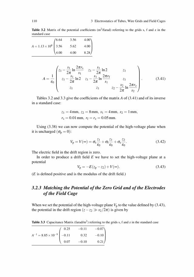
110 3 Electrostatics of Tubes, Wire Grids and Field Cages
Table 3.2 Matrix of the potential coefficients (m2/farad) referring to the grids s, f and z in thestandard case
A = 1.13×10⁸
⎛⎜⎜⎝
6.64 3.56 4.00
3.56 5.62 4.00
4.00 4.00 8.28
⎞⎟⎟⎠
A =1ε0
⎛⎜⎜⎜⎜⎜⎝
z1 −s1
2πln
2πrs
s1z1 −
s1
2πln2 z1
z1 −s1
2πln2 z1 −
s1
2πln
2πrf
s1z1
z1 z1 z2 −s2
2πln
2πrz
s2
⎞⎟⎟⎟⎟⎟⎠
. (3.41)
Tables 3.2 and 3.3 give the coefficients of the matrix A of (3.41) and of its inversein a standard case:
z1 = 4mm, z2 = 8mm, s1 = 4mm, s2 = 1mm,
rs = 0.01mm, rf = rz = 0.05mm.
Using (3.38) we can now compute the potential of the high-voltage plane whenit is uncharged (σp = 0):
Vp = V (∞) = σsz1
ε0+σf
z1
ε0+σz
z2
ε0. (3.42)
The electric field in the drift region is zero.In order to produce a drift field E we have to set the high-voltage plane at a
potentialVp = −E(zp − z2)+V (∞). (3.43)
(E is defined positive and is the modulus of the drift field.)
3.2.3 Matching the Potential of the Zero Grid and of the Electrodesof the Field Cage
When we set the potential of the high-voltage plane Vp to the value defined by (3.43),the potential in the drift region (z− z2 � s2/2π) is given by
Table 3.3 Capacitance Matrix (farad/m2) referring to the grids s, f and z in the standard case
A−1 = 8.85×10⁻⁹
⎛⎜⎜⎝
0.25 −0.11 −0.07
−0.11 0.32 −0.10
0.07 −0.10 0.21
⎞⎟⎟⎠
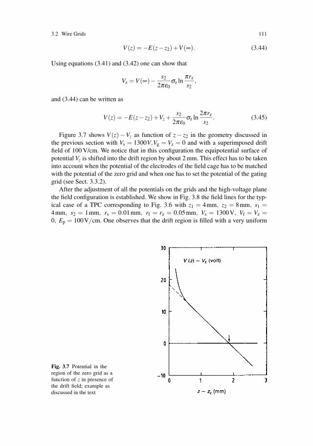
3.2 Wire Grids 111
V (z) = −E(z− z2)+V (∞). (3.44)
Using equations (3.41) and (3.42) one can show that
Vz = V (∞)− s2
2πε0σz ln
πrz
s2,
and (3.44) can be written as
V (z) = −E(z− z2)+Vz +s2
2πε0σz ln
2πrz
s2. (3.45)
Figure 3.7 shows V (z)−Vz as function of z− z2 in the geometry discussed inthe previous section with Vs = 1300V,Vg = Vz = 0 and with a superimposed driftfield of 100 V/cm. We notice that in this configuration the equipotential surface ofpotential Vz is shifted into the drift region by about 2 mm. This effect has to be takeninto account when the potential of the electrodes of the field cage has to be matchedwith the potential of the zero grid and when one has to set the potential of the gatinggrid (see Sect. 3.3.2).
After the adjustment of all the potentials on the grids and the high-voltage planethe field configuration is established. We show in Fig. 3.8 the field lines for the typ-ical case of a TPC corresponding to Fig. 3.6 with z1 = 4mm, z2 = 8mm, s1 =4mm, s2 = 1mm, rs = 0.01mm, rf = rz = 0.05mm, Vs = 1300V, Vf = Vz =0, Ep = 100V/cm. One observes that the drift region is filled with a very uniform
Fig. 3.7 Potential in theregion of the zero grid as afunction of z in presence ofthe drift field; example asdiscussed in the text
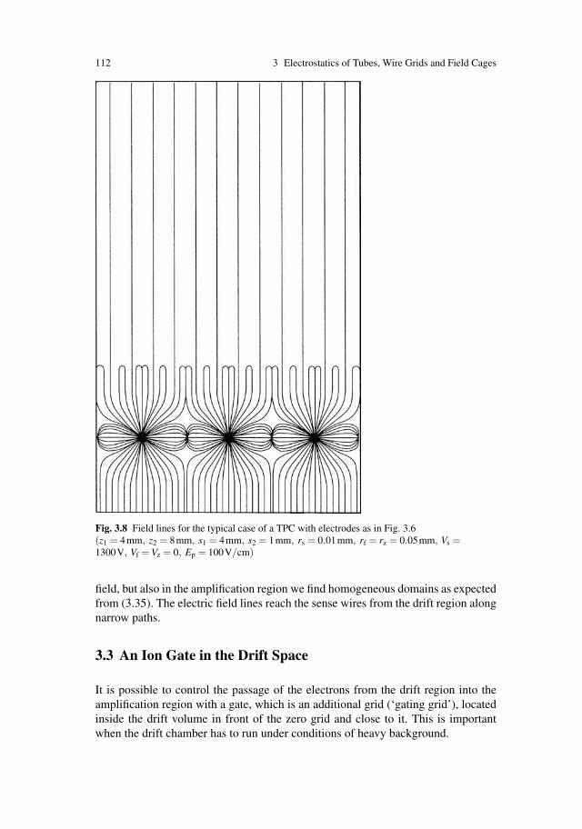
112 3 Electrostatics of Tubes, Wire Grids and Field Cages
Fig. 3.8 Field lines for the typical case of a TPC with electrodes as in Fig. 3.6(z1 = 4mm, z2 = 8mm, s1 = 4mm, s2 = 1mm, rs = 0.01mm, rf = rz = 0.05mm, Vs =1300V, Vf = Vz = 0, Ep = 100V/cm)
field, but also in the amplification region we find homogeneous domains as expectedfrom (3.35). The electric field lines reach the sense wires from the drift region alongnarrow paths.
3.3 An Ion Gate in the Drift Space
It is possible to control the passage of the electrons from the drift region into theamplification region with a gate, which is an additional grid (‘gating grid’), locatedinside the drift volume in front of the zero grid and close to it. This is importantwhen the drift chamber has to run under conditions of heavy background.
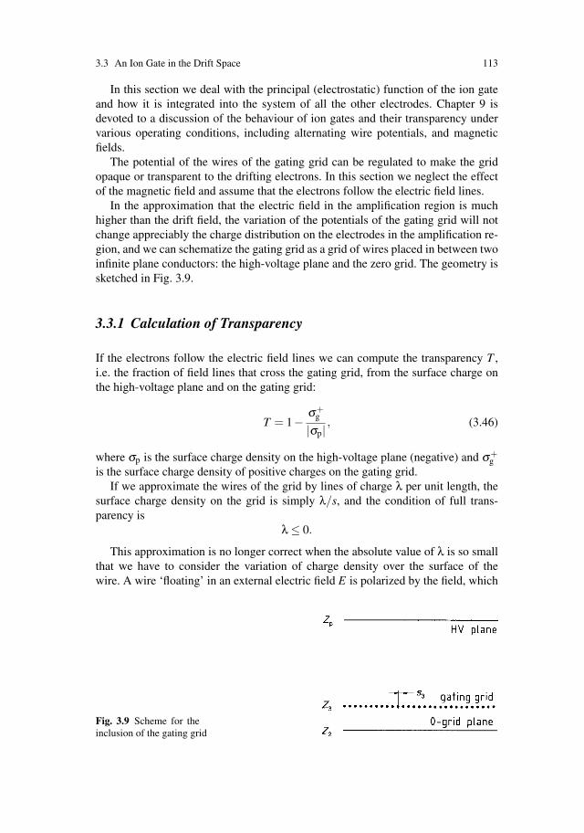
3.3 An Ion Gate in the Drift Space 113
In this section we deal with the principal (electrostatic) function of the ion gateand how it is integrated into the system of all the other electrodes. Chapter 9 isdevoted to a discussion of the behaviour of ion gates and their transparency undervarious operating conditions, including alternating wire potentials, and magneticfields.
The potential of the wires of the gating grid can be regulated to make the gridopaque or transparent to the drifting electrons. In this section we neglect the effectof the magnetic field and assume that the electrons follow the electric field lines.
In the approximation that the electric field in the amplification region is muchhigher than the drift field, the variation of the potentials of the gating grid will notchange appreciably the charge distribution on the electrodes in the amplification re-gion, and we can schematize the gating grid as a grid of wires placed in between twoinfinite plane conductors: the high-voltage plane and the zero grid. The geometry issketched in Fig. 3.9.
3.3.1 Calculation of Transparency
If the electrons follow the electric field lines we can compute the transparency T ,i.e. the fraction of field lines that cross the gating grid, from the surface charge onthe high-voltage plane and on the gating grid:
T = 1−σ+
g
|σp|, (3.46)
where σp is the surface charge density on the high-voltage plane (negative) and σ+g
is the surface charge density of positive charges on the gating grid.If we approximate the wires of the grid by lines of charge λ per unit length, the
surface charge density on the grid is simply λ/s, and the condition of full trans-parency is
λ ≤ 0.
This approximation is no longer correct when the absolute value of λ is so smallthat we have to consider the variation of charge density over the surface of thewire. A wire ‘floating’ in an external electric field E is polarized by the field, which
Fig. 3.9 Scheme for theinclusion of the gating grid
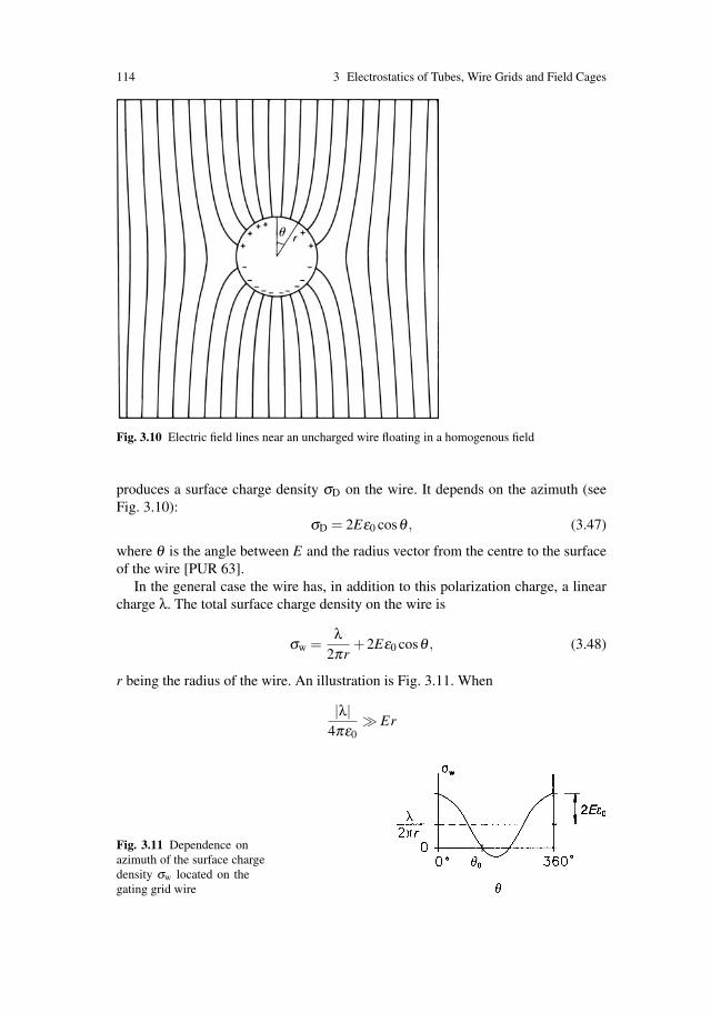
114 3 Electrostatics of Tubes, Wire Grids and Field Cages
Fig. 3.10 Electric field lines near an uncharged wire floating in a homogenous field
produces a surface charge density σD on the wire. It depends on the azimuth (seeFig. 3.10):
σD = 2Eε0 cosθ , (3.47)
where θ is the angle between E and the radius vector from the centre to the surfaceof the wire [PUR 63].
In the general case the wire has, in addition to this polarization charge, a linearcharge λ. The total surface charge density on the wire is
σw =λ
2πr+2Eε0 cosθ , (3.48)
r being the radius of the wire. An illustration is Fig. 3.11. When
|λ|4πε0
� Er
Fig. 3.11 Dependence onazimuth of the surface chargedensity σw located on thegating grid wire
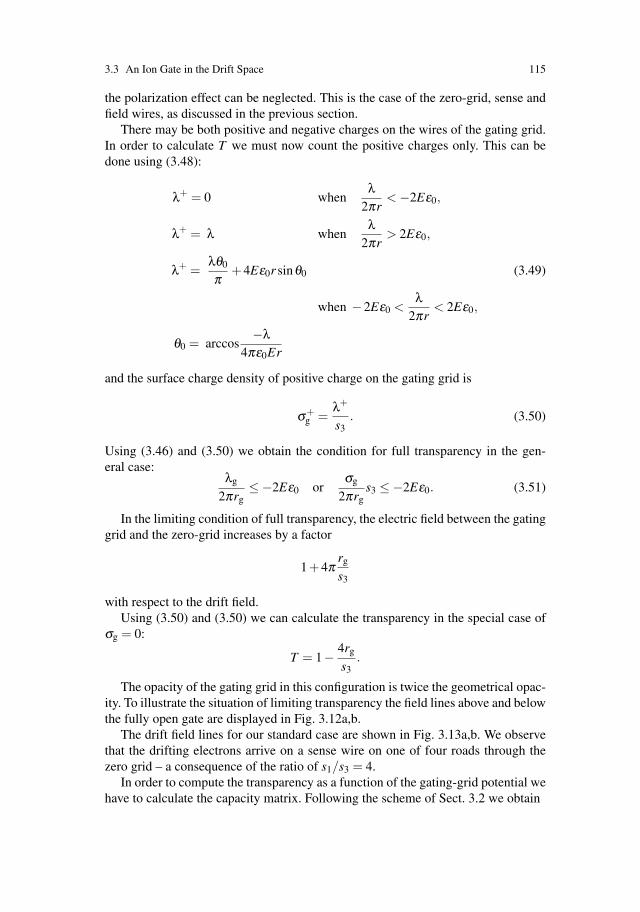
3.3 An Ion Gate in the Drift Space 115
the polarization effect can be neglected. This is the case of the zero-grid, sense andfield wires, as discussed in the previous section.
There may be both positive and negative charges on the wires of the gating grid.In order to calculate T we must now count the positive charges only. This can bedone using (3.48):
λ+ = 0 whenλ
2πr< −2Eε0,
λ+ = λ whenλ
2πr> 2Eε0,
λ+ =λθ0
π+4Eε0r sinθ0 (3.49)
when −2Eε0 <λ
2πr< 2Eε0,
θ0 = arccos−λ
4πε0Er
and the surface charge density of positive charge on the gating grid is
σ+g =
λ+
s3. (3.50)
Using (3.46) and (3.50) we obtain the condition for full transparency in the gen-eral case:
λg
2πrg≤−2Eε0 or
σg
2πrgs3 ≤−2Eε0. (3.51)
In the limiting condition of full transparency, the electric field between the gatinggrid and the zero-grid increases by a factor
1+4πrg
s3
with respect to the drift field.Using (3.50) and (3.50) we can calculate the transparency in the special case of
σg = 0:
T = 1− 4rg
s3.
The opacity of the gating grid in this configuration is twice the geometrical opac-ity. To illustrate the situation of limiting transparency the field lines above and belowthe fully open gate are displayed in Fig. 3.12a,b.
The drift field lines for our standard case are shown in Fig. 3.13a,b. We observethat the drifting electrons arrive on a sense wire on one of four roads through thezero grid – a consequence of the ratio of s1/s3 = 4.
In order to compute the transparency as a function of the gating-grid potential wehave to calculate the capacity matrix. Following the scheme of Sect. 3.2 we obtain
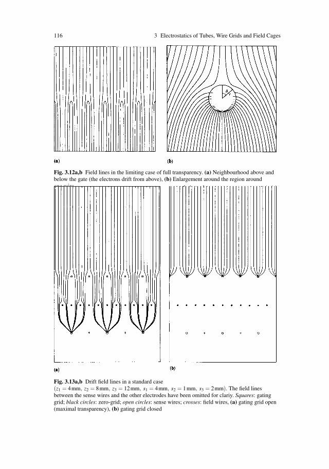
116 3 Electrostatics of Tubes, Wire Grids and Field Cages
Fig. 3.12a,b Field lines in the limiting case of full transparency. (a) Neighbourhood above andbelow the gate (the electrons drift from above), (b) Enlargement around the region aroundone wire
Fig. 3.13a,b Drift field lines in a standard case(z1 = 4mm, z2 = 8mm, z3 = 12mm, s1 = 4mm, s2 = 1mm, s3 = 2mm). The field linesbetween the sense wires and the other electrodes have been omitted for clariy. Squares: gatinggrid; black circles: zero-grid; open circles: sense wires; crosses: field wires, (a) gating grid open(maximal transparency), (b) gating grid closed
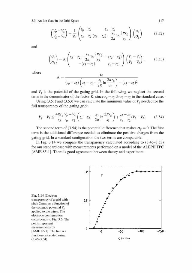
3.3 An Ion Gate in the Drift Space 117
(Vp −Vz
Vg −Vz
)=
1ε0
⎛⎝zp − z2 z3 − z2
z3 − z2 (z3 − z2)−s3
2πln
2πrg
s3
⎞⎠(σp
σg
)(3.52)
and
(σp
σg
)= K
⎛⎝z3 − z2 −
s3
2πln
2πrg
s3−(z3 − z2)
−(z3 − z2) zp − z2
⎞⎠(Vp −Vz
Vg −Vz
), (3.53)
whereK =
ε0
(zp − z2)(
z3 − z2 −s3
2πln
2πrg
s3
)− (z3 − z2)2
and Vg is the potential of the gating grid. In the following we neglect the secondterm in the denominator of the factor K, since zp− z2 � z3− z2 in the standard case.
Using (3.51) and (3.53) we can calculate the minimum value of Vg needed for thefull transparency of the gating grid:
Vg −Vz ≤4πrg
s3
Vp −Vz
zp − z2
(z3 − z2 −
s3
2πln
2πrg
s3
)+
z3 − z2
zp − z2(Vp −Vz). (3.54)
The second term of (3.54) is the potential difference that makes σg = 0. The firstterm is the additional difference needed to eliminate the positive charges from thegating grid. In a standard configuration the two terms are comparable.
In Fig. 3.14 we compare the transparency calculated according to (3.46–3.53)for our standard case with measurements performed on a model of the ALEPH TPC[AME 85-1]. There is good agreement between theory and experiment.
Fig. 3.14 Electrontransparency of a grid withpitch 2 mm, as a function ofthe common potential Vgapplied to the wires. Theelectrode configurationcorresponds to Fig. 3.6. Thepoints representmeasurements by[AME 85-1]. The line is afunction calculated using(3.46–3.54)
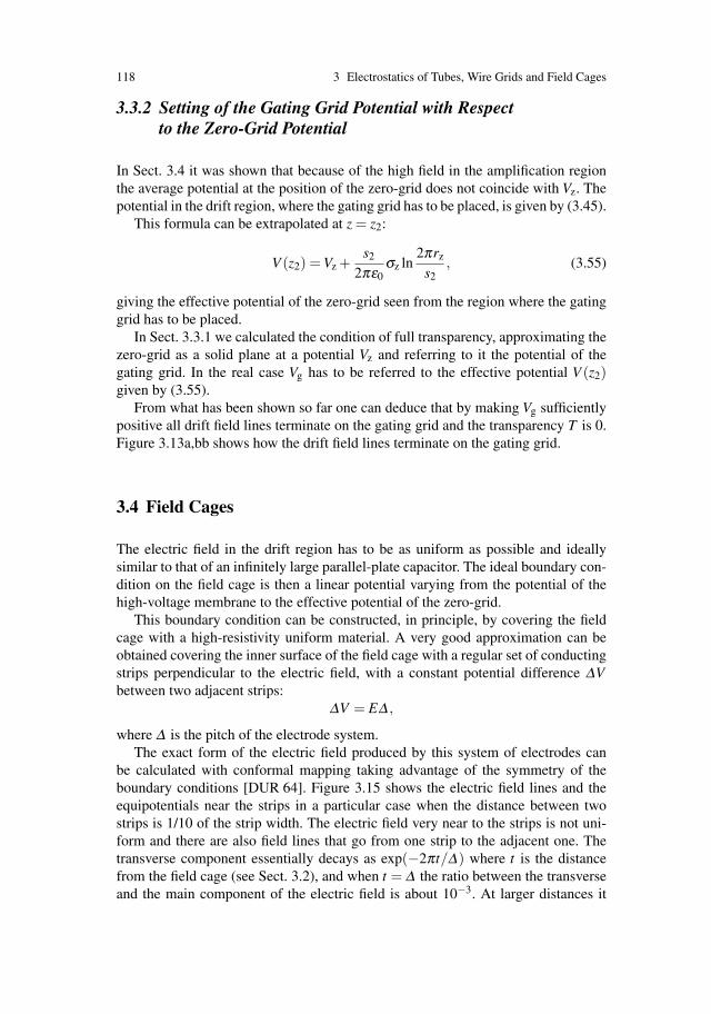
118 3 Electrostatics of Tubes, Wire Grids and Field Cages
3.3.2 Setting of the Gating Grid Potential with Respectto the Zero-Grid Potential
In Sect. 3.4 it was shown that because of the high field in the amplification regionthe average potential at the position of the zero-grid does not coincide with Vz. Thepotential in the drift region, where the gating grid has to be placed, is given by (3.45).
This formula can be extrapolated at z = z2:
V (z2) = Vz +s2
2πε0σz ln
2πrz
s2, (3.55)
giving the effective potential of the zero-grid seen from the region where the gatinggrid has to be placed.
In Sect. 3.3.1 we calculated the condition of full transparency, approximating thezero-grid as a solid plane at a potential Vz and referring to it the potential of thegating grid. In the real case Vg has to be referred to the effective potential V (z2)given by (3.55).
From what has been shown so far one can deduce that by making Vg sufficientlypositive all drift field lines terminate on the gating grid and the transparency T is 0.Figure 3.13a,bb shows how the drift field lines terminate on the gating grid.
3.4 Field Cages
The electric field in the drift region has to be as uniform as possible and ideallysimilar to that of an infinitely large parallel-plate capacitor. The ideal boundary con-dition on the field cage is then a linear potential varying from the potential of thehigh-voltage membrane to the effective potential of the zero-grid.
This boundary condition can be constructed, in principle, by covering the fieldcage with a high-resistivity uniform material. A very good approximation can beobtained covering the inner surface of the field cage with a regular set of conductingstrips perpendicular to the electric field, with a constant potential difference ΔVbetween two adjacent strips:
ΔV = EΔ ,
where Δ is the pitch of the electrode system.The exact form of the electric field produced by this system of electrodes can
be calculated with conformal mapping taking advantage of the symmetry of theboundary conditions [DUR 64]. Figure 3.15 shows the electric field lines and theequipotentials near the strips in a particular case when the distance between twostrips is 1/10 of the strip width. The electric field very near to the strips is not uni-form and there are also field lines that go from one strip to the adjacent one. Thetransverse component essentially decays as exp(−2πt/Δ) where t is the distancefrom the field cage (see Sect. 3.2), and when t = Δ the ratio between the transverseand the main component of the electric field is about 10−3. At larger distances it
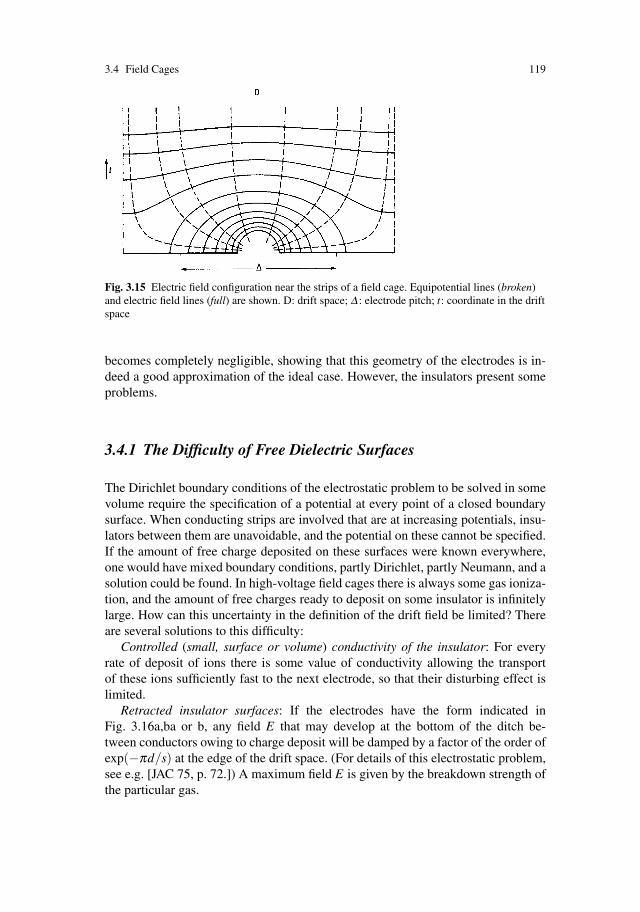
3.4 Field Cages 119
Fig. 3.15 Electric field configuration near the strips of a field cage. Equipotential lines (broken)and electric field lines (full) are shown. D: drift space; Δ : electrode pitch; t: coordinate in the driftspace
becomes completely negligible, showing that this geometry of the electrodes is in-deed a good approximation of the ideal case. However, the insulators present someproblems.
3.4.1 The Difficulty of Free Dielectric Surfaces
The Dirichlet boundary conditions of the electrostatic problem to be solved in somevolume require the specification of a potential at every point of a closed boundarysurface. When conducting strips are involved that are at increasing potentials, insu-lators between them are unavoidable, and the potential on these cannot be specified.If the amount of free charge deposited on these surfaces were known everywhere,one would have mixed boundary conditions, partly Dirichlet, partly Neumann, and asolution could be found. In high-voltage field cages there is always some gas ioniza-tion, and the amount of free charges ready to deposit on some insulator is infinitelylarge. How can this uncertainty in the definition of the drift field be limited? Thereare several solutions to this difficulty:
Controlled (small, surface or volume) conductivity of the insulator: For everyrate of deposit of ions there is some value of conductivity allowing the transportof these ions sufficiently fast to the next electrode, so that their disturbing effect islimited.
Retracted insulator surfaces: If the electrodes have the form indicated inFig. 3.16a,ba or b, any field E that may develop at the bottom of the ditch be-tween conductors owing to charge deposit will be damped by a factor of the order ofexp(−πd/s) at the edge of the drift space. (For details of this electrostatic problem,see e.g. [JAC 75, p. 72.]) A maximum field E is given by the breakdown strength ofthe particular gas.

120 3 Electrostatics of Tubes, Wire Grids and Field Cages
Fig. 3.16a,b Field-cageelectrode configuration withretracted insulator surfaces.I: insulator, C: conductor, D:drift space, (a) small gap, (b)large gap
Thin insulator with shielding electrodes covering the gap from behind: Apartfrom the system of main electrodes, there is another set separated by a thin layer ofinsulator, and staggered by a half-step according to Fig. 3.17. The purpose of theseshielding electrodes at intermediate potentials is to regularize the field in the driftregion, but also to produce virtual mirror charges of any free charges that may havedeposited in the gap, thus reducing their effect in the drift space.
If we assume that by one of the measures described above the adverse effectsof any charge deposit are sufficiently reduced, we may imagine a smooth (linear)transition of potential between neighbouring electrodes, and the exact form of theelectric field produced by the system of electrodes at increasing potentials can becalculated as discussed at the beginning of this section.
Electrostatic distortions were studied by Iwasaki et al. [IWA 83].
Fig. 3.17 Field-cage electrode configuration with secondary electrode strips (SE) covering thegaps between the main electrode strips (ME) behind a thin insulator foil (It). D: drift space; I:insulator

3.4 Field Cages 121
3.4.2 Irregularities in the Field Cage
In this subsection we present some studies that have arisen in practice when estimat-ing the tolerances that had to be respected in the ALEPH TPC for the conductivityof the insulator, for the match of the gating grid and for the resistors in the potentialdivider. We quote the three relevant electrostatic solutions as examples of similarproblems in chambers with different geometry.
If all the electrodes of the field cage are set at the correct potential, the drift fieldis uniform and parallel to the axis of the TPC in the whole drift volume. A wrongsetting of the potentials produces a transverse component of the electric field andcauses a distortion of the trajectories of the drifting electrons. In order to study thiseffect in detail the drift volume of the TPC is schematized as a cylinder of length Land radius A (see Fig. 3.18). The potentials defined on the surface of the cylinderdefine the boundary conditions of the electrostatic problem and the drift field insidethe volume. If the potentials on the boundary do not vary with φ , the electric fieldcan only have a transverse component in the radial direction.
In the absence of magnetic field the electrons drift along the electric field line; anelectron placed at the position (r0, z0) reaches the end of the drift volume at a radialposition
r = r0 +0∫
z0
Er(r,z)Ez
dz.
The radial component of the field can be calculated solving the Poisson equation incylindrical coordinates [JAC 75, p. 108]. Since the ideal setting of the potential doesnot produce radial electric field components it is convenient to use as a boundarycondition the difference between the actual and the ideal potentials. This is possiblebecause the Poisson equation is linear in the potential. Although we discuss the ex-amples in a cylindrical geometry, they apply to other geometries in a similar way.
Non-Linearity in the Resistor Chain. The potential of the strips of the field cage aredefined connecting them to a linear resistor chain. The strips are insulated from theexternal ground by an insulator that has a finite resistivity and that is in parallel withthe resistors of the chain. It can be shown that the resistance to ground of a stripplaced at a position z is
Fig. 3.18 Scheme of acylindrical TPC drift region
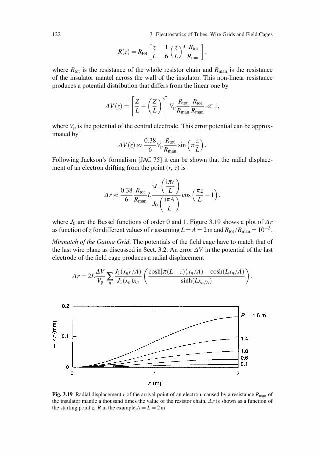
122 3 Electrostatics of Tubes, Wire Grids and Field Cages
R(z) = Rtot
[zL− 1
6
( zL
)3 Rtot
Rman
],
where Rtot is the resistance of the whole resistor chain and Rman is the resistanceof the insulator mantel across the wall of the insulator. This non-linear resistanceproduces a potential distribution that differs from the linear one by
ΔV (z) =
[ZL−(
ZL
)3]
VpRtot
Rman
Rtot
Rman 1,
where Vp is the potential of the central electrode. This error potential can be approx-imated by
ΔV (z) ≈ 0.386
VpRtot
Rmansin(
πzL
).
Following Jackson’s formalism [JAC 75] it can be shown that the radial displace-ment of an electron drifting from the point (r, z) is
Δr ≈ 0.386
Rtot
RmanL
iJ1
(iπrL
)
J0
(iπAL
) cos(πz
L−1)
,
where J0 are the Bessel functions of order 0 and 1. Figure 3.19 shows a plot of Δras function of z for different values of r assuming L = A = 2m and Rtot/Rman = 10−3.
Mismatch of the Gating Grid. The potentials of the field cage have to match that ofthe last wire plane as discussed in Sect. 3.2. An error ΔV in the potential of the lastelectrode of the field cage produces a radial displacement
Δr = 2LΔVVp
∑n
J1(xnr/A)J1(xn)xn
(cosh[π(L− z)(xn/A)− cosh(Lxn/A)
sinh(Lxn/A)
),
Fig. 3.19 Radial displacement r of the arrival point of an electron, caused by a resistance Rman ofthe insulator mantle a thousand times the value of the resistor chain, Δr is shown as a function ofthe starting point z, R in the example A = L = 2m

3.4 Field Cages 123
Fig. 3.20 Radial displacement Δr of the arrival point of an electron, caused by a voltage mismatchΔV between the last electrode of the field cage and the last wire plane, amounting to ΔV/Vp = 10−4
of the drift voltage. Δr is shown as a function of the starting point (z, R) in the example A = L = 2m
where xn = knA and J0(kn) = 0.Figure 3.20 shows a plot of Δr as a function of z for different values of r assuming
L = A = 2m and ΔV/Vp = 10−4.Resistor Chain Containing One Wrong Resistor. If in the voltage-divider chain oneof the resistors (placed at z = z) has a wrong value, it induces an error in the potentialof the field cage:
ΔV (z) =−ΔV
Lz, z < z,
ΔV(
1− zL
), z > z,
ΔV = VpΔRRtot
,
where ΔR is the error in the resistance of that particular resistor and Rtot is the totalresistance of the chain. The induced radial displacement is
Fig. 3.21 Radial displacement Δr of the arrival point of an electron, caused by one wrong resistorvalue R∗ = R+ΔR, where ΔR/Rtot = 1/400 of the value of the total resistor chain. Δr is shown asa function of the starting point (z, R) in the example A = L = 2m
124 3 Electrostatics of Tubes, Wire Grids and Field Cages
Δr = LΔRrtot
[1π ∑ iJ1(inπr)/L
J0(inπA)/L1n
cos
(nπ zL
)(cos
nπzL
−1)]
.
Figure 3.21 shows a plot of Δr as a function of z for different values of r for aparticular case L = A = 2m, z = 1.4m, ΔR/Rtot = 1/400.
We have computed in this subsection three specific cases of field-cage prob-lems in the spirit of showing the order of magnitude of the relevant electrondisplacements. The design of the drift chamber must be such that the displace-ment Δr induced by such irregularities remains small in comparison to the requiredaccuracy.
References
[ABR 65] M. Abramowitz and I.A. Stegun, Handbook of Mathematical Functions, (Dover,New York 1965) p. 75
[AME 85-1] S.R. Amendolia et al., Influence of the magnet field on the gating of a time projectionchamber, Nucl. Instrum. Methods A 234, 47 (1985)
[DUR 64] Durand, Electrostatique vol. II (Masson et C. edts., Paris 1964)[FAB 04] C.W. Fabjan and W. Riegler, Trends and Highlights of VCI 2004, Nucl. Instr. Meth.
Phys. Res. A 535, p. 79-87 (2004)[IWA 83] H. Iwasaki, R.J. Maderas, D.R. Nygren, G.T. Przybylski, and R.R. Sauerwein,
Studies of electrostatic distortions with a small time projection chamber, in The TimeProjection Chamber (A.I.P. Conference Proceedings No. 10 TRIUMF, Vancouver,Canada, 1983)
[JAC 75] J.D. Jackson, Classical Electrodynamics (Wiley, New York 1975)[MOR 53] P.M. Morse and H. Feshbach, Methods of Theoretical Physics (McGraw Hill,
New York 1953).[PUR 63] E.M. Purcell, Electricity and Magnetism (Berkeley Physics Course Vol. II, McGraw
Hill, New York 1963) Problem 9.11[VEN 08] R. Veenhof, Drift Chamber Simulation Program Garfield, (1984–2008)[WEN 58] G. Wendt, Statische Felder und stationare Strome in Handbuch der Physik, Vol. XVI
(Springer, Berlin Heidelberg 1958) p. 148
Chapter 4Amplification of Ionization
4.1 The Proportional Wire
Among all the amplifiers of the feeble energy deposited by a particle on its passagethrough matter, the proportional wire is a particularly simple and well-known exam-ple. When it is coupled with a sensitive electronic amplifier, a few – even single –electrons from the ionization of a particle can be observed, which create ionizationavalanches in the high electric field near the surface of the thin wire. The develop-ment of the proportional counter started as long ago as 1948; for an early review,see [CUR 58]. The proportional counter is also treated in text books on counters ingeneral, for example those of Korff [KOR 55] and Knoll [KNO 79]. The latter con-tains a basic list of reference texts. The classical monograph by Raether [RAE 64]deals with electron avalanches in a broader context.
As an electron drifts towards the wire it travels in an increasing electric field E,which, in the vicinity of the wire at radius r, is given by the linear charge density λon the wire:
E =λ
2πε0
1r
.
In the absence of a magnetic field, the path of the electron will be radial. Thepresence of a magnetic field modifies the path (as discussed in Chaps. 2 and 7) but,if the electric field is strong enough, the trajectory terminates in any case on thewire.
Once the electric field near the electron is strong enough so that between colli-sions with the gas molecules the electron can pick up sufficient energy for ionization,another electron is created and the avalanche starts. At normal gas density the meanfree path between two collisions is of the order of microns; hence the field that startsthe avalanche is of the order of several 104 V/cm, and the wire has to be thin, say afew 10−3 cm, for 1 or 2 kV.
As the number of electrons multiplies in successive generations (Fig. 4.1), theavalanche continues to grow until all the electrons are collected on the wire. Theavalanche does not, in general, surround the wire but develops preferentially onthe approach side of the initiating electrons (cf. Sect. 4.3). The whole process
W. Blum et al., Particle Detection with Drift Chambers, 125doi: 10.1007/978-3-540-76684-1 4, c© Springer-Verlag Berlin Heidelberg 2008

126 4 Amplification of Ionization
Fig. 4.1 Schematicdevelopment of theproportional wire avalanche
develops in the longitudinal direction over as many free paths as there are gener-ations, say typically over 50 to 100μm. This part ends after a fraction of a nanosec-ond, under normal gas conditions. The physical processes inside the avalancheare quite complicated, as they involve single and multiple ionization, optical andmetastable excitations, perhaps recombinations, and energy transfer by collisionsbetween atoms, much the same as discussed in Sect. 1.1. The de-excitation ofmetastable states may in principle increase the duration of the avalanche up tothe collision time between the molecules, but not much is known aboutthis.
The proportional wire owes its name to the fact that the signal is proportionalto the number of electrons collected. This proportionality is possible to the extentthat the avalanche-induced changes of the electric field remain negligible comparedto the field of the wire. Referring to Sect. 4.5.1, we may characterize the regimeof proportionality as that in which the charge density in the avalanche is negligi-ble compared with the linear charge density of the wire. The charge density of theavalanche is given by the product of the gain factor and the number of electrons thatstart the avalanche, divided by its width.
A very interesting role is played by the photons, which are as abundant as elec-trons because the relevant cross-sections are of the same order of magnitude. Asmall fraction of them will be energetic enough to ionize the gas, in all probabilityionizing a gas component with a low ionization potential. If it now happens thatthese ionizing photons travel further, on the average, than the longitudinal size of
Fig. 4.2 Mechanism ofbreakdown byphotoionization of the gasoutside the cylinder thatcontains the full avalanche

4.1 The Proportional Wire 127
the avalanche, then the electrons they produce will each give rise to another fullavalanche and the counter may break down. In order to formulate a stability crite-rion, we refer to the avalanche of Fig. 4.2, created by one electron e1. Let us call ne
the number of electrons in the avalanche and nph the number of energetic photons,and use q to denote the average probability that one of them ionizes the gas outsidethe radius rmin. Breakdown occurs if
nphq > 1 , xneq > 1 ,
where x is the ratio nph/ne. This ratio may be expected to stay roughly constant asne is changed by a variation of the wire voltage.
Fig. 4.3a,b Optical properties of chamber gases: (a) Outstanding spectral emission lines of theneutral Ar atom [HAN 81]. The intensities are approximate and are plotted on a logarithmic scale.(b) Absorption cross-sections for UV photons of the normal alkanes [SCH 62]

128 4 Amplification of Ionization
Table 4.1 Common quench gases
Methane CH4Ethane C2H6Propane C3H8Butane C4H10Pentane C5H12Isobutane (CH3)2CHCH3Carbon dioxide CO2Ethylene (C2H2)2Methylal CH2(CH2OH)2
A similar consideration applies also to photons from the avalanche that reach theconducting surfaces of the cathodes, where they may create free electrons by thephotoelectric effect.
It is because of these far-travelling photons that an organic ‘quench gas’ needsto be present. Its effect is to reduce q allowing larger values of ne, and hence largergain. Organic molecules, with their many degrees of freedom, have large photoab-sorption coefficients over a range of wavelengths that is wider than that for noblegas atoms. Some examples are given in Fig. 4.3a,b, which also contains a picture ofthe most prominent emission lines of the argon. The photoabsorption spectrum ofargon was shown as a graph in Fig. 1.4 in the context of a calculation of particle ion-ization. Table 4.1 contains a list of common quench gases. Inorganic quench gaseshave been studied by Dwurazny, Jelen, and Rulikowska–Zabrebska [DWU 83].
4.2 Beyond the Proportional Mode
If the avalanche amplification is increased beyond the region of proportionality, thespace charge of the positive ions reduces appreciably the field near the head of theavalanche, that is the field experienced by the electrons between the wire and thepositive cloud. The amplification is smaller for any subsequent increment and weare in the regime of ‘limited proportionality’.
Near the tail of the avalanche, however, we have an increase of the electricfield owing to the positive ions, especially once the fast-moving electrons havedisappeared into the wire. This situation leads to two different kinds of multiplica-tive processes, depending on the behaviour of the photons:
• If the UV absorption of the quench gas is very strong, the photons in theavalanche produce ionization near their creation point, including the region nearthe tail of the avalanche where the electric field is particularly large. This startsthe phenomenon of the ‘limited streamer’, which is a backward-moving multipli-cation process in the sense of a series of avalanches whose starting points movefurther and further away from the wire. In a paper by Atac, Tollestrup, and Potter[ATA 82], it is suggested that energetic photons are created by the recombinationprocess with cool electrons when the field at the avalanche head is sufficiently
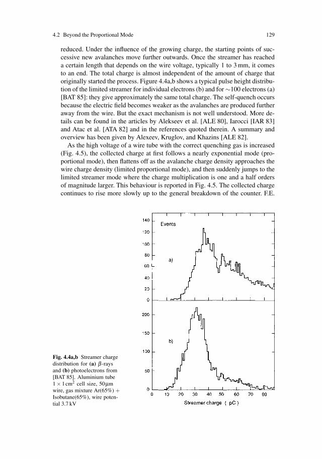
4.2 Beyond the Proportional Mode 129
reduced. Under the influence of the growing charge, the starting points of suc-cessive new avalanches move further outwards. Once the streamer has reacheda certain length that depends on the wire voltage, typically 1 to 3 mm, it comesto an end. The total charge is almost independent of the amount of charge thatoriginally started the process. Figure 4.4a,b shows a typical pulse height distribu-tion of the limited streamer for individual electrons (b) and for ∼100 electrons (a)[BAT 85]: they give approximately the same total charge. The self-quench occursbecause the electric field becomes weaker as the avalanches are produced furtheraway from the wire. But the exact mechanism is not well understood. More de-tails can be found in the articles by Alekseev et al. [ALE 80], Iarocci [IAR 83]and Atac et al. [ATA 82] and in the references quoted therein. A summary andoverview has been given by Alexeev, Kruglov, and Khazins [ALE 82].
As the high voltage of a wire tube with the correct quenching gas is increased(Fig. 4.5), the collected charge at first follows a nearly exponential mode (pro-portional mode), then flattens off as the avalanche charge density approaches thewire charge density (limited proportional mode), and then suddenly jumps to thelimited streamer mode where the charge multiplication is one and a half ordersof magnitude larger. This behaviour is reported in Fig. 4.5. The collected chargecontinues to rise more slowly up to the general breakdown of the counter. F.E.
Fig. 4.4a,b Streamer chargedistribution for (a) β -raysand (b) photoelectrons from[BAT 85]. Aluminium tube1× 1cm2 cell size, 50μmwire, gas mixture Ar(65%) +Isobutane(65%), wire poten-tial 3.7 kV

130 4 Amplification of Ionization
Fig. 4.5 Collected chargeas a function of the highvoltage, measured by Atacet al. [ATA 82] on a 100μmdiameter wire in a tube12 × 12mm2, filled withAr(49.3%)+C2H6(49.3%)+CH3CH2OH(1.4%)
Taylor argues that the size of the limited streamer is essentially given by electro-static considerations [TAY 90].
• If the UV absorption of the gas is so low that ionizing photons can travel distancesthat are comparable to the counter dimension, then multiplicative processes maydevelop along the full length of the wire. The wire is said to be in Geiger modeif the external electric circuit terminates the discharge with the help of a largeHV feed resistor. The size of the signal is therefore also independent of theoriginal charge. The Geiger counter is described, for example, in [KNO 79] and[KOR 55].
4.3 Lateral Extent of the Avalanche
The electrons from an ionization track, which are collected on a wire and start anavalanche there, do not usually arrive at the same point in space, but there is somespread between them. This happens not only because the track was originally ex-tended in space, and every electron is guided on its drift path to a different placenear the wire, but also because of the diffusion in the gas during the drift. The pro-portional avalanche has a lateral extent that is at least as large as this spread.
In the avalanche process itself there is a lateral development associated with themultiplication of charges, and this is mainly due to diffusion of electrons, the elec-trostatic repulsion of charges, and the propagation of ionizing photons. The intrinsiclateral size of an avalanche therefore depends on the gas (collision cross-section and
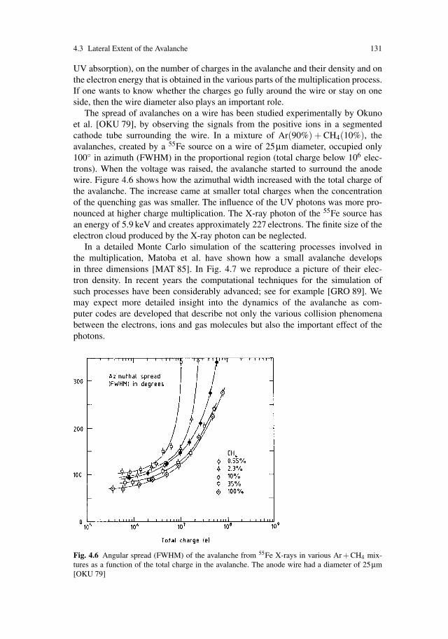
4.3 Lateral Extent of the Avalanche 131
UV absorption), on the number of charges in the avalanche and their density and onthe electron energy that is obtained in the various parts of the multiplication process.If one wants to know whether the charges go fully around the wire or stay on oneside, then the wire diameter also plays an important role.
The spread of avalanches on a wire has been studied experimentally by Okunoet al. [OKU 79], by observing the signals from the positive ions in a segmentedcathode tube surrounding the wire. In a mixture of Ar(90%) + CH4(10%), theavalanches, created by a 55Fe source on a wire of 25μm diameter, occupied only100◦ in azimuth (FWHM) in the proportional region (total charge below 106 elec-trons). When the voltage was raised, the avalanche started to surround the anodewire. Figure 4.6 shows how the azimuthal width increased with the total charge ofthe avalanche. The increase came at smaller total charges when the concentrationof the quenching gas was smaller. The influence of the UV photons was more pro-nounced at higher charge multiplication. The X-ray photon of the 55Fe source hasan energy of 5.9 keV and creates approximately 227 electrons. The finite size of theelectron cloud produced by the X-ray photon can be neglected.
In a detailed Monte Carlo simulation of the scattering processes involved inthe multiplication, Matoba et al. have shown how a small avalanche developsin three dimensions [MAT 85]. In Fig. 4.7 we reproduce a picture of their elec-tron density. In recent years the computational techniques for the simulation ofsuch processes have been considerably advanced; see for example [GRO 89]. Wemay expect more detailed insight into the dynamics of the avalanche as com-puter codes are developed that describe not only the various collision phenomenabetween the electrons, ions and gas molecules but also the important effect of thephotons.
Fig. 4.6 Angular spread (FWHM) of the avalanche from 55Fe X-rays in various Ar + CH4 mix-tures as a function of the total charge in the avalanche. The anode wire had a diameter of 25μm[OKU 79]
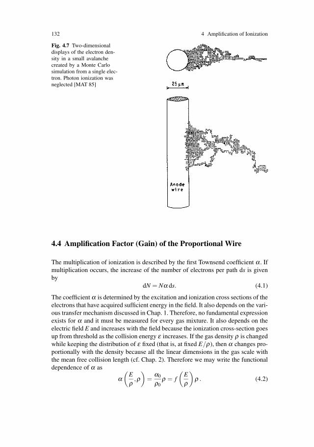
132 4 Amplification of Ionization
Fig. 4.7 Two-dimensionaldisplays of the electron den-sity in a small avalanchecreated by a Monte Carlosimulation from a single elec-tron. Photon ionization wasneglected [MAT 85]
4.4 Amplification Factor (Gain) of the Proportional Wire
The multiplication of ionization is described by the first Townsend coefficient α . Ifmultiplication occurs, the increase of the number of electrons per path ds is givenby
dN = Nα ds. (4.1)
The coefficient α is determined by the excitation and ionization cross sections of theelectrons that have acquired sufficient energy in the field. It also depends on the vari-ous transfer mechanism discussed in Chap. 1. Therefore, no fundamental expressionexists for α and it must be measured for every gas mixture. It also depends on theelectric field E and increases with the field because the ionization cross-section goesup from threshold as the collision energy ε increases. If the gas density ρ is changedwhile keeping the distribution of ε fixed (that is, at fixed E/ρ), then α changes pro-portionally with the density because all the linear dimensions in the gas scale withthe mean free collision length (cf. Chap. 2). Therefore we may write the functionaldependence of α as
α(
Eρ
,ρ)
=α0
ρ0ρ = f
(Eρ
)ρ . (4.2)
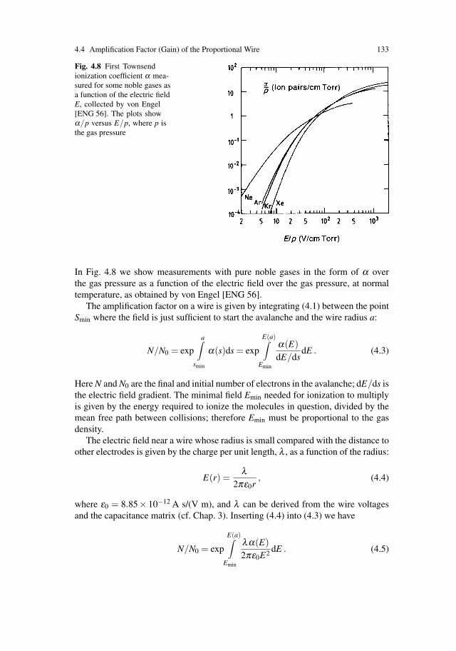
4.4 Amplification Factor (Gain) of the Proportional Wire 133
Fig. 4.8 First Townsendionization coefficient α mea-sured for some noble gases asa function of the electric fieldE, collected by von Engel[ENG 56]. The plots showα/p versus E/p, where p isthe gas pressure
In Fig. 4.8 we show measurements with pure noble gases in the form of α overthe gas pressure as a function of the electric field over the gas pressure, at normaltemperature, as obtained by von Engel [ENG 56].
The amplification factor on a wire is given by integrating (4.1) between the pointSmin where the field is just sufficient to start the avalanche and the wire radius a:
N/N0 = exp
a∫smin
α(s)ds = exp
E(a)∫Emin
α(E)dE/ds
dE . (4.3)
Here N and N0 are the final and initial number of electrons in the avalanche; dE/ds isthe electric field gradient. The minimal field Emin needed for ionization to multiplyis given by the energy required to ionize the molecules in question, divided by themean free path between collisions; therefore Emin must be proportional to the gasdensity.
The electric field near a wire whose radius is small compared with the distance toother electrodes is given by the charge per unit length, λ , as a function of the radius:
E(r) =λ
2πε0r, (4.4)
where ε0 = 8.85× 10⁻¹² A s/(V m), and λ can be derived from the wire voltagesand the capacitance matrix (cf. Chap. 3). Inserting (4.4) into (4.3) we have
N/N0 = exp
E(a)∫Emin
λα(E)2πε0E2 dE . (4.5)

134 4 Amplification of Ionization
The ratio N/N0 is usually called gain. In the following paragraphs we use G =N/N0 to indicate it.
4.4.1 The Diethorn Formula
Diethorn [DIE 56] derived a useful formula for G by assuming α to be proportionalto E. Looking at Fig. 4.8, this is not unreasonable for heavy noble gases between102 and 103 [V/cm Torr], a typical range of fields near thin wires. Inserting α = βEinto (4.5) gives
lnG =βλ
2πε0ln
λ2πε0aEmin
. (4.6)
The value of β can be related in the following way to the average energy eΔVrequired to produce one more electron. The potential difference between r = a andr = smin that corresponds to relation (4.3) is
Φ(a)−Φ(Smin) =Smin∫a
E(r)dr =λ
2πε0ln
Smin
a=
λ2πε0
lnλ
2πε0aEmin. (4.7)
It gives rise to a number Z of generations of doubling the electrons in the avalanche:
Z = [Φ(a)−Φ(Smin)]/ΔV , (4.8)
G = 2Z , (4.9)
lnG =ln2ΔV
λ2πε0
lnλ
2πε0aEmin. (4.10)
We recognize that in this model the constant β of (4.6) has the meaning of theinverse of the average potential required to produce one electron in the avalanchemultiplied by ln 2.We write Emin, which is proportional to the gas density ρ , in the form
Emin(ρ) = Emin(ρ0)ρρ0
, (4.11)
where ρ0 is the normal gas density. We finally obtain
lnG =ln2ΔV
λ2πε0
lnλ
2πε0aEmin(ρ0)(ρ/ρ0). (4.12)
Relation (4.12) was compared with measurements using proportional countertubes, and was shown to be better than the older models of Rose–Korff and Curran–Craggs; see [HEN 72, WOL 74, KIS 60] and the literature quoted therein. In aproportional counter tube with inner radius b and wire radius a, the charge densityλ is related to the voltage V by

4.4 Amplification Factor (Gain) of the Proportional Wire 135
λ2πε0
=V
ln(b/a). (4.13)
Therefore, (4.12) can also be expressed in the following form (Diethorn’s formula):
lnG =ln2
ln(b/a)V
ΔVln
Vln(b/a)aEmin(ρ0)(ρ/ρ0)
. (4.14)
Experimentally, we vary ρ/ρ0,a and V/ ln(b/a), and measure G. A plot of
lnG ln(b/a)V
versus lnV
ln(b/a)a(ρ/ρ0)
must be linear and yields the two constants Emin(ρ0) and ΔV . Figure 4.9 showssuch a plot made by Hendricks [HEN 72] for two xenon gas mixtures, and Table 4.2contains a collection of Diethorn parameters measured in this way, typically foramplification factors between 102 and 105. They are only in moderate agreementwith each other.
We recognize the value of formulae (4.12) and (4.14), discussed above, morefrom a practical than from a fundamental point of view. Obviously, for a given gasmixture, the Townsend coefficient α(E) must first be known accurately as a functionof the electric field. Then the multiplication factor can be calculated using (4.5). Seealso Charles [CHA 72] and Shalev and Hopstone [SHA 78], who compared andcriticized various formulae for the gas gain.
Fig. 4.9 Diethorn plot ofamplification measurementsusing two Xe gas mixtures[HEN 72]; p = ρ/ρ0
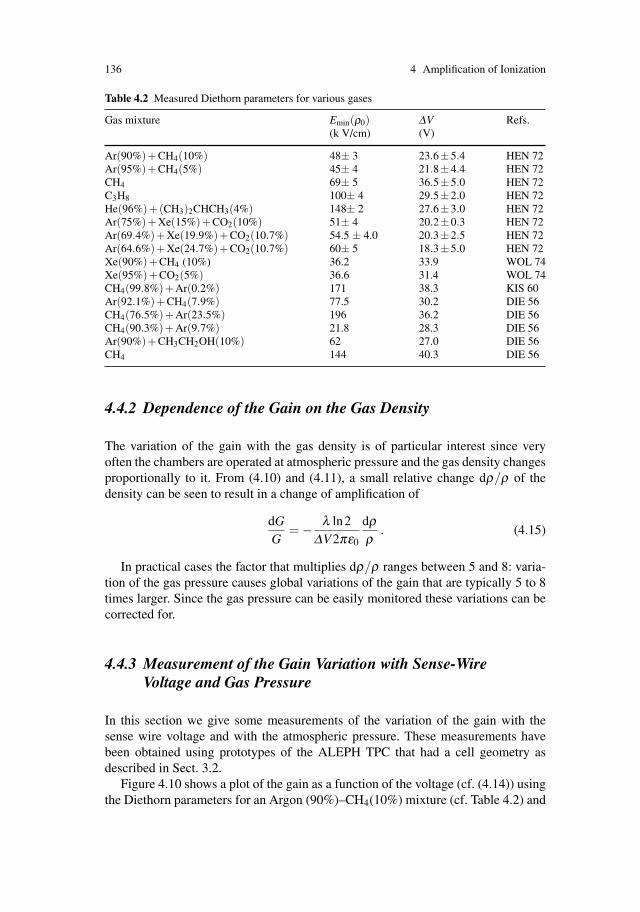
136 4 Amplification of Ionization
Table 4.2 Measured Diethorn parameters for various gases
Gas mixture Emin(ρ0) ΔV Refs.(k V/cm) (V)
Ar(90%)+CH4(10%) 48± 3 23.6±5.4 HEN 72Ar(95%)+CH4(5%) 45± 4 21.8±4.4 HEN 72CH4 69± 5 36.5±5.0 HEN 72C3H8 100± 4 29.5±2.0 HEN 72He(96%)+(CH3)2CHCH3(4%) 148± 2 27.6±3.0 HEN 72Ar(75%)+Xe(15%)+CO2(10%) 51± 4 20.2±0.3 HEN 72Ar(69.4%)+Xe(19.9%)+CO2(10.7%) 54.5 ± 4.0 20.3±2.5 HEN 72Ar(64.6%)+Xe(24.7%)+CO2(10.7%) 60± 5 18.3±5.0 HEN 72Xe(90%)+CH4 (10%) 36.2 33.9 WOL 74Xe(95%)+CO2(5%) 36.6 31.4 WOL 74CH4(99.8%)+Ar(0.2%) 171 38.3 KIS 60Ar(92.1%)+CH4(7.9%) 77.5 30.2 DIE 56CH4(76.5%)+Ar(23.5%) 196 36.2 DIE 56CH4(90.3%)+Ar(9.7%) 21.8 28.3 DIE 56Ar(90%)+CH3CH2OH(10%) 62 27.0 DIE 56CH4 144 40.3 DIE 56
4.4.2 Dependence of the Gain on the Gas Density
The variation of the gain with the gas density is of particular interest since veryoften the chambers are operated at atmospheric pressure and the gas density changesproportionally to it. From (4.10) and (4.11), a small relative change dρ/ρ of thedensity can be seen to result in a change of amplification of
dGG
= − λ ln2ΔV2πε0
dρρ
. (4.15)
In practical cases the factor that multiplies dρ/ρ ranges between 5 and 8: varia-tion of the gas pressure causes global variations of the gain that are typically 5 to 8times larger. Since the gas pressure can be easily monitored these variations can becorrected for.
4.4.3 Measurement of the Gain Variation with Sense-WireVoltage and Gas Pressure
In this section we give some measurements of the variation of the gain with thesense wire voltage and with the atmospheric pressure. These measurements havebeen obtained using prototypes of the ALEPH TPC that had a cell geometry asdescribed in Sect. 3.2.
Figure 4.10 shows a plot of the gain as a function of the voltage (cf. (4.14)) usingthe Diethorn parameters for an Argon (90%)–CH4(10%) mixture (cf. Table 4.2) and

4.4 Amplification Factor (Gain) of the Proportional Wire 137
Fig. 4.10 Gain as a functionof the sense-wire voltage in achamber with a cell geometryas described in Sect. 3.2. Dotsare measurements done witha model of the ALEPH TPC;the full line is computed with(4.14) and Table 4.2; brokenlines show the error marginsintroduced by the error inTable 4.2
assuming atmospheric pressure. The two side-lines show the large uncertainty inthe prediction of the gain owing to the large error (20%) in ΔV . The superimposedexperimental points have been measured with a chamber under the same operatingconditions. The agreement is very good.
Figure 4.11 shows the variation of the atmospheric pressure p over a period of2 days (a) and the corresponding average pulse height measured by the chamberwhen detecting the electrons produced in the gas by the absorption of X-rays froma 55Fe source (b). One notices how the measured pulse height follows the variationsof the pressure (note the zero-suppressed scales of the two plots). The chamberwas operated in an Argon (90%)–CH4(10%) mixture. The sense-wire voltage was1.4 kV and the field wires were grounded. Using Table 3.5 we can compute thelinear charge density λ of the sense wires and from the measured value of ΔV
Fig. 4.11 (a) Atmospheric pressure p as a function of the time in a time interval of two days. (b)Average pulse-height measured by the chamber in the same period. Measurements done with theALEPH TPC
138 4 Amplification of Ionization
(cf. Table 4.2) using (4.15) we predict that
dGG
= −(6.7±1.5)dpp
.
Inspecting Fig. 4.11 a we read an overall change of pressure of 0.8% and predict achange of gain of −(5.5±1.2)%, in agreement with the variation (−4%) shown inFig. 4.11b.
4.5 Local Variations of the Gain
Equation (4.12) shows that the gain depends on the local charge density of the wireλ . A relative change dλ/λ , as may result from geometrical imperfections of a wirechamber, from fluctuations of the supply voltage, or from space charge near the wirewill change the amplification by the factor [cf. (4.12)]
dGG
=(
lnG+λ ln2
ΔV 2πε0
)dλλ
. (4.16)
In practical cases the two factors in the parentheses of the previous equation are ofthe same order of magnitude and their sum lies in the range 10–20: the local relativevariations of the charge density cause local relative variations of the gain that aretypically 10–20 times greater.
In Sect. 3.2 we saw how the linear charge density λ depends on the potentialsand on the geometry of the wire chamber, assuming that there is an ideal geometry.Real chambers deviate from the ideal geometry: the wires are not infinite and wecan expect changes in the charge density in the region close to the wire supports.Moreover, the mechanical components of the chamber have small construction im-perfections, which can induce local changes in the charge density along the wire.The mathematical solution of the electrostatic problem is not simple because assoon as we introduce variations in the ideal geometry we lose the symmetry of theboundary conditions.
In drift chambers that are operated in high-density particle fluxes there is anotherproblem: the local charge density on the wire seen by ionization electrons when theyreach the wire can be modified by the presence of the ions which were produced ina previous avalanche and still are drifting inside the drift cell.
4.5.1 Variation of the Gain Near the Edge of the Chamber
In wire chambers the gain usually drops to zero near the support frame. This be-haviour depends on the details of the geometry and extends over a region of thewire comparable to the distance between the sense-wire grid and the cathode plane.
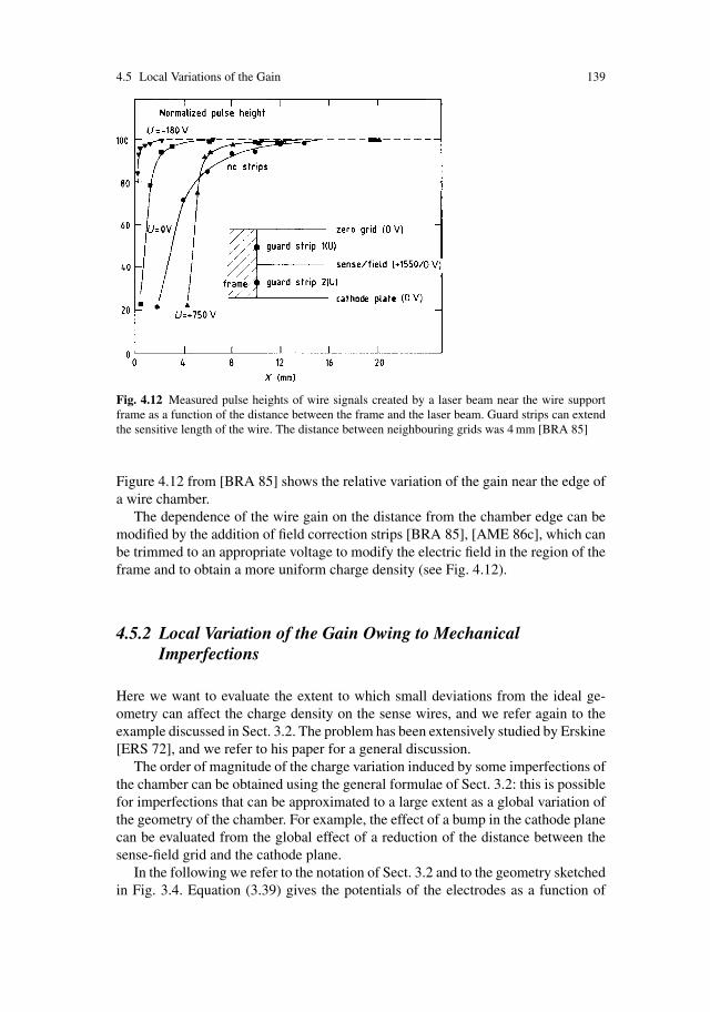
4.5 Local Variations of the Gain 139
Fig. 4.12 Measured pulse heights of wire signals created by a laser beam near the wire supportframe as a function of the distance between the frame and the laser beam. Guard strips can extendthe sensitive length of the wire. The distance between neighbouring grids was 4 mm [BRA 85]
Figure 4.12 from [BRA 85] shows the relative variation of the gain near the edge ofa wire chamber.
The dependence of the wire gain on the distance from the chamber edge can bemodified by the addition of field correction strips [BRA 85], [AME 86c], which canbe trimmed to an appropriate voltage to modify the electric field in the region of theframe and to obtain a more uniform charge density (see Fig. 4.12).
4.5.2 Local Variation of the Gain Owing to MechanicalImperfections
Here we want to evaluate the extent to which small deviations from the ideal ge-ometry can affect the charge density on the sense wires, and we refer again to theexample discussed in Sect. 3.2. The problem has been extensively studied by Erskine[ERS 72], and we refer to his paper for a general discussion.
The order of magnitude of the charge variation induced by some imperfections ofthe chamber can be obtained using the general formulae of Sect. 3.2: this is possiblefor imperfections that can be approximated to a large extent as a global variation ofthe geometry of the chamber. For example, the effect of a bump in the cathode planecan be evaluated from the global effect of a reduction of the distance between thesense-field grid and the cathode plane.
In the following we refer to the notation of Sect. 3.2 and to the geometry sketchedin Fig. 3.4. Equation (3.39) gives the potentials of the electrodes as a function of
140 4 Amplification of Ionization
their charges and of the matrix of the potential coefficients A:
V = Aσ , (4.17)
where the σi = λi/Si are the linear charge densities on the wires of each grid dividedby the pitch of the grid. A change in the geometry of the wire chamber induces achange in the matrix. Differentiating (4.17) with the fixed values of the potential V,we obtain
Adσ = −dAσ ,
where dσ is the vector of the charge-density variations and dA is the matrix ofthe variations in the potential coefficients induced by a particular change in thegeometry of the chamber. Using the previous equation, we obtain
dσ = −A−1dAσ . (4.18)
As a first example we calculate the charge-density variation induced by a dis-placement of the cathode plane. The matrix dA can be calculated by differentiating(3.41) with respect to z, noting that the effect of a displacement dz of the cathodeplane changes z1 and z2 by the same amount (cf. Fig. 3.4):
dA = −dzε0
⎛⎜⎜⎝
1 1 1
1 1 1
1 1 1
⎞⎟⎟⎠ . (4.19)
From (4.18),
dσ =dzε0
A−1
⎛⎜⎜⎝
σs +σF +σz
σs +σF +σz
σs +σF +σz
⎞⎟⎟⎠ . (4.20)
In the approximations of Sect. 3.2 the quantity σs + σF + σz is the charge densityon the cathode plane. The charge-density variation dσ induced by a displacementof the cathode plane vanishes if there are no charges on the plane. In the particulargeometry of the example considered in Sect. 3.2, we obtain:
dσs = (70m)−1dz(σs +σF +σz) .
As another example we now compute the charge variation induced by a change inthe sense-wire diameter. Differentiating (3.41) with respect to the sense-wire radiusrs yields
dA = − s1
2πε0
drs
rs
⎛⎜⎜⎝
1 0 0
0 0 0
0 0 0
⎞⎟⎟⎠ , (4.21)

4.5 Local Variations of the Gain 141
and
dσ = − s1
2πε0
drs
rsA−1
⎛⎜⎜⎝
σs
0
0
⎞⎟⎟⎠ . (4.22)
For the particular example considered in Sect. 3.2 we get
dσs
σs= 0.16
drs
rs.
The effect of the displacement of a single wire is more difficult. In this case wecannot use (3.41) because it was calculated for a set of symmetric grids, and thissymmetry is lost when a single wire is displaced. We note that in first order thedisplacement of a wire does not affect the charge density of the wire itself (againbecause of the symmetry), but only that of other wires close to it. The displacementof a field wire changes the charge density of the two closest sense wires proportion-ally to its own charge density. If there is no charge density on the field wires, theirdisplacement does not affect the gain of the chamber.
Table 4.3 shows the gain variations induced by mechanical imperfections in thegeometry of the example discussed here. We have assumed that the setting of thevoltages produces a gain of 104, and using (4.16) we compute the relation betweenthe relative variation of the gain and the local relative charge-density variation:
dGG
= (15.9±1.5)dσs
σs.
The same gain can be obtained for different settings of the sense-wire voltage(Vs) and the field-wire voltage (VF) that leave the charge density on the sense wireσs unchanged. Using Table 3.3 we compute the condition of constant gain:
0.25Vs −0.11VF = constant .
The different settings correspond to different values of the ratio σF/σs. Again usingTable 3.3 we deduce that if VF/Vs = 0, then σF/σs = −0.44, while σF/σs = 0 whenVF/Vs = 0.34. As shown in Table 4.3 the ratio σF/σs influences the local variationsof the gain that are due to mechanical imperfections.
Table 4.3 Gain variation dG/G induced by mechanical imperfections in the geometry discussedin Sect. 3.2. A gain of 104 is assumed and all displacements (Δ ) are in mm. σF/σs is the ratiobetween the charge densities on the field wires and the sense wires
Imperfection dG/G
Bump on the pad plane 0.69Δz(1+σF/σs)Displacement of a field wire 1.1ΔxσF/σsDisplacement of a sense wire 0.2ΔxVariation of the sense wire diameter 2.5Δr/r

142 4 Amplification of Ionization
4.5.3 Gain Drop due to Space Charge
When the avalanche has come to an end, all electrons are collected on the anode andthe space near the wire is filled with the remaining positive ions. We may assumethat in the regime of proportional wire amplification, the amount of charge in theavalanche is small compared to the charge on the wire (integrated along the wireover the lateral extent of the avalanche). The positive ions are moving away fromthe wire at relatively low speed. With a mobility of a few cm/s per V/cm, a typicalspeed near the thin wire (E ∼ 2 × 10⁵ V/cm) would be several 105 cm/s, and ahundred times less at a hundred times the radius. The avalanche charge obviouslytakes hundreds of microseconds to settle on a cathode several millimetres away.
When there is a continuous particle flow with a much higher frequency than thatcorresponding to the ion travel time, we have a stationary situation, and the travel-ling ions build up a stationary space charge density ρ(x) in the chamber volume.This reduces the electric field close to the wire and therefore the gas gain, whichposes a fundamental limitation on the rate capability of any wire chamber.
In order to calculate ρ we consider in Figure 4.13 a small area A1 of the wiresurface which shows an electric field E1 and which releases positive ions of chargeq at a constant rate ν . The ions are moving with a velocity of v = μE1 where μ isthe ion mobility. Within a time Δ t, the charge Q1 = qν Δ t is entering the volumeV1 = A1vΔ t, which results in a charge density of ρ1 = Q1/V1 = qν/μE1A1 close tothe wire surface. As the ions are moving away from the wire along the electric fieldlines they are passing an equipotential area A2 in a field E2, and the charge densityat this position is ρ2 = qν/μE2A2. From Gauss’ Law we know that E2A2 −E1A1 =Q/ε0, where Q is the total charge contained in the ‘flux tube’ between A1 and A2.If the electric field due to the space charge is small compared to the electric field
A1, E1
A2, E2
A3, E3
Fig. 4.13 Anode wire with some field lines (continuous) and some equipotential lines (broken).The A’s symbolize the areas of the equipotential surfaces between the same field lines that comefrom the border of the original area A1 on the wire surface. The E’s represent the fields on theequipotential surfaces. As the ions travel along the field lines they become slower by the samefactor as the field lines go apart, resulting in a constant charge density in the volume (‘flux tube’)filled with ions originating from A1
4.5 Local Variations of the Gain 143
from the wire, which is usually the case, we may neglect Q and obtain in first orderthat
E1A1 = E2A2 and therefore ρ1 = ρ2.
We have found the remarkable result that the charge density is constant along theentire ‘flux tube’ at any distance from the wire. In case the electric field E1 andthe ion flux ν are uniform around the wire surface, which is a common case, wefind a constant charge density in the entire volume that is filled by the field linesoriginating from the wire.
For a wire of radius a with a surface field of E1, a charge deposit q at a rate of Rper unit length of the wire we therefore find a uniform space charge density of
ρ =qR
μE12aπ. (4.23)
Next we investigate the gas gain drop due to the presence of ρ . Setting a wire topotential V0 amounts to placing a certain charge λ on the wire. The charge density ρcreates an electric field Es(x) which is superimposed on the electric field of the wirecharge λ . The resulting potential difference due to ρ is ΔV =
∫Es(x)ds, where the
path of integration is taken from the wire surface to the cathode. Consequently thewire charge λ is reduced such that its contribution to the potential is V0 −ΔV . Thegain reduction due to the space charge ρ is therefore equal to a voltage reductionof ΔV in the absence of space charge. This effective voltage drop of the wires in achamber is therefore calculated in first order by removing all wires and calculatingthe potential difference between wire positions and cathode due to the charge densityρ . We will now discuss two examples.
First we examine a drift tube (cf. Section 3.1) exposed to a particle flux of Φ perunit detector area and a total avalanche charge of q per particle. With R = 2bΦ andthe wire surface field of E1 = V0/(a ln b
a ) we find the uniform space charge density
ρ =bqΦ ln b
a
πμV0. (4.24)
In the absence of the wire, ρ produces an electric field of Es(r) = ρr/2ε0, so thepotential difference between wire position and tube wall is
ΔV =∫ b
0Es(r)dr = ρb2/4ε0 =
b3qΦ ln ba
4πε0μV0. (4.25)
The voltage drop is proportional to the third power of the tube radius, so a reductionof the tube radius is the most effective way to increase the rate capability. As anexample, Fig. 4.14 shows the gain reduction in the drift tubes of the ATLAS muonspectrometer [ATL 00]. The measurements are well explained by the theory outlinedabove.
As a second example we investigate a wire chamber schematically shown inFig. 4.15, where a row of wires with a pitch of s is positioned symmetrically be-tween two grounded cathode planes at a distance h. Setting all wires to potential V0,
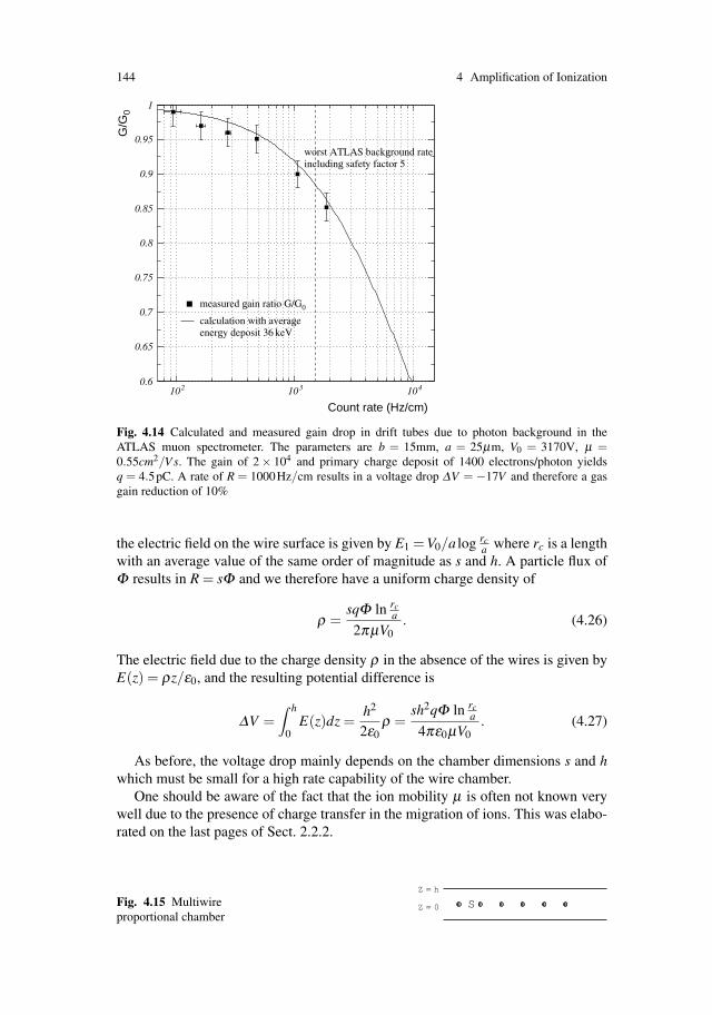
144 4 Amplification of Ionization
0.6
0.65
0.7
0.75
0.8
0.85
0.9
0.95
1
10
310
2 10
4
Count rate (Hz/cm)
G/G
0
worst ATLAS background rateincluding safety factor 5
calculation with averageenergy deposit 36 keV
measured gain ratio G/G0
Fig. 4.14 Calculated and measured gain drop in drift tubes due to photon background in theATLAS muon spectrometer. The parameters are b = 15mm, a = 25μm, V0 = 3170V, μ =0.55cm2/V s. The gain of 2 × 10⁴ and primary charge deposit of 1400 electrons/photon yieldsq = 4.5pC. A rate of R = 1000Hz/cm results in a voltage drop ΔV = −17V and therefore a gasgain reduction of 10%
the electric field on the wire surface is given by E1 =V0/a log rca where rc is a length
with an average value of the same order of magnitude as s and h. A particle flux ofΦ results in R = sΦ and we therefore have a uniform charge density of
ρ =sqΦ ln rc
a
2πμV0. (4.26)
The electric field due to the charge density ρ in the absence of the wires is given byE(z) = ρz/ε0, and the resulting potential difference is
ΔV =∫ h
0E(z)dz =
h2
2ε0ρ =
sh2qΦ ln rca
4πε0μV0. (4.27)
As before, the voltage drop mainly depends on the chamber dimensions s and hwhich must be small for a high rate capability of the wire chamber.
One should be aware of the fact that the ion mobility μ is often not known verywell due to the presence of charge transfer in the migration of ions. This was elabo-rated on the last pages of Sect. 2.2.2.
Fig. 4.15 Multiwireproportional chamber
SZ = h
Z = 0
4.6 Statistical Fluctuation of the Gain 145
4.6 Statistical Fluctuation of the Gain
The gain of an avalanche is equal to the number of ion pairs within it divided bythe number of electrons that started the avalanche. In the regime of proportionality,the average number of electrons produced in the avalanche is proportional to thenumber of initial electrons. We are interested in the fluctuation in the number ofelectrons that is caused by the random nature of the multiplication process.
We may assume that each initiating electron develops its own small avalanche,independent of the presence of the others nearby. If we want to know the probabil-ity distribution of the number N of the ions in the total avalanche we simply sumover the probability distribution P(n) of the number n of electrons in the individualsmall avalanches. The first step is to find an expression P(n), which is done in thefollowing sections.
If the number k of initiating electrons is large, the central-limit theorem of statis-tics, which makes a statement about the distribution function F(N) of the sum N,applies:
N = n1 +n2 +n3 + . . .+nk, (4.28)
where each of the independent variables ni has the distribution function P(n). If themean of P(n) is called n and the variance is σ2, then the central-limit theorem statesthat in the limit of k → ∞, F(N) is a Gaussian:
F(N) =1
S√
2πexp[(N −N)2/2S2] (4.29)
withN = kn and S2 = k σ2 . (4.30)
This means that the exact shape of P(n) is not needed for the distribution ofavalanches started by a large number of electrons. On the other hand, P(n) is par-ticularly interesting for drift chambers where individual ionization electrons have tobe detected, as in ring-imaging (RICH) counters.
Single-electron spectra and avalanche fluctuations in proportional counters havebeen measured by Hurst et al., using laser resonant ionization spectroscopy (RIS)[HUR 78] and by Schlumbohm [SCH 58], whose data are discussed later. A reviewof single-electron spectra is given by Genz [GEN 73].
Statistical fluctuations of the gain may be influenced by chemical reactions asso-ciated with the formation of avalanches. Such deterioration of performance occurseither through deposits on old wires or through the presence of small contaminationsof the gas. A discussion of these effects is given in Sect. 12.6; we refer especially toFig. 12.7. Here we assume that the proportional wire is in an unperturbed workingcondition.
4.6.1 Distributions of Avalanches in Weak Fields
In this section we investigate the fluctuation of avalanches started by single elec-trons in weak electric fields, where the assumption holds that the average distance
146 4 Amplification of Ionization
between ionizing collisions 1/α is large compared to the distance x0 = Ui/E whichan electron of zero energy has to travel before reaching the ionization potential Ui
of the gas [SNY 47] [WIJ 49] [LEG 55]. In this case the probability for an ionizingcollision in a spatial interval ds is p = αds, independent of the electron’s ‘history’(see Sect. 4.6.3 for details). We assume a single electron starting at position s = 0and moving along a coordinate s, where it experiences an electric field E(s) and aTownsend coefficient α(s). Equation 4.3 tells us that at position s we will find onaverage n(s) = exp(
∫ s0 α(s′)ds′) electrons. Since the multiplication is a statistical
process, the true number will fluctuate around this average, and we are looking forP(n,s), the probability of finding n electrons at a position s. With the above assump-tions (p = αds), we have the following probability of finding n electrons at positions+ds:
P(n,s+ds) = P(n−1,s)(n−1)p(1− p)n−2 +P(n,s)(1− p)n (4.31)
The first term on the right-hand side represents the probability that we find n− 1electrons at s and exactly one of them duplicates; the second term represents theprobability that there are already n electrons and no duplication takes place. Allother possibilities are of order ds2 and higher. Expanding the above expression forsmall values of ds yields the equation
dP(n,s)ds
= P(n−1,s)(n−1)α(s)−P(n,s)nα(s), (4.32)
with the conditions P(1,0) = 1 and P(n,0) = 0 for n > 1. If we write the equationin terms of a transformed variable u =
∫ s0 α(s′)ds′, it assumes the simpler form
dP(n,u)du
= P(n−1,u)(n−1)−P(n,u)n. (4.33)
For the beginning of the process, we have the equation
dP(1,u)du
= −P(1,u) and therefore P(1,u) = e−u. (4.34)
The probabilities for n > 0 are calculated by inserting P(1,u) into Eq. (4.32) anditerating the procedure, which yields
P(n,u) = e−u(1− e−u)n−1. (4.35)
Returning to the variable s, we finally get
P(n,s) =1
n(s)
(1− 1
n(s)
)n−1
n(s) = exp(∫ s
0α(s′)ds′). (4.36)
We see that the probability distribution depends only on n and not explicitly ons, which means that the avalanche distribution has the same shape at every stageof the avalanche and for any coordinate dependence of α . The variance of the

4.6 Statistical Fluctuation of the Gain 147
distribution is
σ(s)2 =∞
∑n=1
n2P(n,s)−n(s)2 = n(s)(n(s)−1) . (4.37)
In the limit of n → ∞, which is quite appropriate for avalanches, the expressionsbecome
P(n,s) =1
n(s)e− n
n(s) σ(s) = n(s). (4.38)
The equations tell us that the avalanche process has an exponential signal dis-tribution, small signals being most probable, and that the r.m.s. width is equal tothe mean (Yule-Furry law). The pulse-height distribution is purely monotonic andshows no peak. This is actually confirmed by experiment; see the measurementsdescribed in Sect. 4.6.3 (Fig. 4.16a).
4.6.2 Distributions of Avalanches in Electronegative Gases
Gases containing electronegative components will attach electrons during the de-velopment of the avalanche and this will affect the gain fluctuations. We thereforeintroduce an attachment coefficient η [LEG 61]. Just as the expression αds repre-sents the probability that an electron experiences an ionizing collision in a spatialinterval ds, forming an electron and a positive ion, the value ηds represents theprobability that an electron attaches in a spatial interval ds, forming a negative ion.The average number of electrons n(s) and positive ions m(s) is therefore defined bythe relation dn = (α −η)nds and dm = αnds, which, for the average number ofelectrons, yields
n(s) = exp∫ s
0(α(s′)−η(s′))ds′ (4.39)
The average number of negative ions is then m− n. The value α −η is called the‘effective’ Townsend coefficient. In order to arrive at the avalanche distribution weproceed as before. There are four possibilities for n electrons to arrive at positions + ds: (1) From n electrons, one multiplies and one attaches; (2) from n electrons,none multiplies and none attaches; (3) from n−1 electrons one multiplies and noneattaches, and (4) from n+1 electrons, none multiplies and one attaches. In first orderof ds this reads as
dP(n,s)ds
= P(n−1,s)(n−1)α −P(n,s)n(α +η)+P(n+1,s)(n+1)η . (4.40)
Since α(s) and η(s) generally have a different functional dependence on theelectric field and thus on s, we cannot transform the equation into a simple form asbefore. We therefore assume α and η to be constant, meaning that the followingsolutions are only valid for a constant electric field. According to Legler [LEG 61]the solution of Eq. (4.40) is

148 4 Amplification of Ionization

4.6 Statistical Fluctuation of the Gain 149
P(n,s) = kn(s)−1n(s)− k
n = 0
= n(s)(
1− kn(s)− k
)2(n(s)−1n(s)− k
)n−1
n > 0
(4.41)
where we have defined k = η/α . The variance of this distribution is σ2 = n(n−1)(1+ k)/(1− k). For large values of n we find P(0,s) = k, and for n > 0 we find
P(n,s) =(1− k)2
n(s)exp
[−(1− k)
nn(s)
]σ2(s) =
1+ k1− k
n(s)2. (4.42)
The attachment therefore results in the probability k = η/α that one ends up withzero electrons. Compared to the situation without attachment, the distribution isstill exponential and the r.m.s. is increased by the factor
√(1+ k)/(1− k). Aver-
aging only over avalanches with n > 0, we find the average number of electronsn∗(x) = n(x)/(1− k) and a variance of σ(x)2 = n∗(x)2. We conclude that the effectof attachment increases the avalanche fluctuations and results again in an exponen-tial signal distribution.
4.6.3 Distributions of Avalanches in Strong Homogeneous Fields
Figure 4.16a-e shows measurements taken in parallel-plate geometry in methylalvapour for five different fields of increasing strength. For a weak field there is thepurely exponential distribution. As the field is increased a depletion at small num-bers of ions is visible, becomes more and more pronounced, and produces a clearpeak at high electric fields. All of these curves display an approximate exponentialdecrease at the upper end which becomes steeper for higher E.
A quantitative explanation of these measurements was given by Legler [LEG 61]in terms of the parameter
χ =α(E)Ui
E, (4.43)
where E is the electric field, α the first Townsend coefficient, and Ui the ioniza-tion potential of the gas. Owing to the dependence of α on E (Fig. 4.8), χ usuallyincreases with increasing E.
The electron that causes an ionizing collision loses at least the energy e0Ui in thecollision, and a new electron with nearly zero energy joins the avalanche. The newelectron has to travel a distance greater than x0 = Ui/E in order to have a non-zeroprobability for ionization. In case this distance x0 is small compared to the average
�Fig. 4.16a-e Distribution of numbers of ions in avalanches started by single electrons as measuredby Schlumbohm [SCH 58] in methylal, in parallel-plate geometry, for various values of χ : (a)χ = 0.038, (b) χ = 0.044, (c) χ = 0.095, (d) χ = 0.19, superimposed on the theoretical curve byLegler, dotted (see text), (e) χ = 0.24
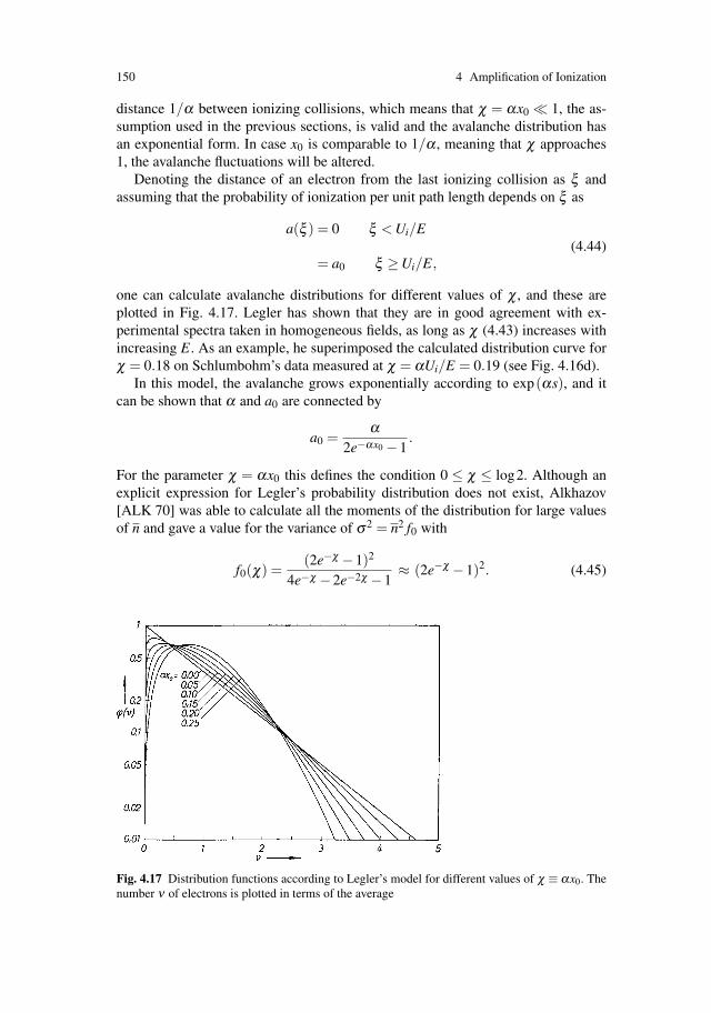
150 4 Amplification of Ionization
distance 1/α between ionizing collisions, which means that χ = αx0 1, the as-sumption used in the previous sections, is valid and the avalanche distribution hasan exponential form. In case x0 is comparable to 1/α , meaning that χ approaches1, the avalanche fluctuations will be altered.
Denoting the distance of an electron from the last ionizing collision as ξ andassuming that the probability of ionization per unit path length depends on ξ as
a(ξ ) = 0 ξ < Ui/E
= a0 ξ ≥Ui/E,(4.44)
one can calculate avalanche distributions for different values of χ , and these areplotted in Fig. 4.17. Legler has shown that they are in good agreement with ex-perimental spectra taken in homogeneous fields, as long as χ (4.43) increases withincreasing E. As an example, he superimposed the calculated distribution curve forχ = 0.18 on Schlumbohm’s data measured at χ = αUi/E = 0.19 (see Fig. 4.16d).
In this model, the avalanche grows exponentially according to exp(αs), and itcan be shown that α and a0 are connected by
a0 =α
2e−αx0 −1.
For the parameter χ = αx0 this defines the condition 0 ≤ χ ≤ log2. Although anexplicit expression for Legler’s probability distribution does not exist, Alkhazov[ALK 70] was able to calculate all the moments of the distribution for large valuesof n and gave a value for the variance of σ2 = n2 f0 with
f0(χ) =(2e−χ −1)2
4e−χ −2e−2χ −1≈ (2e−χ −1)2. (4.45)
Fig. 4.17 Distribution functions according to Legler’s model for different values of χ ≡ αx0. Thenumber ν of electrons is plotted in terms of the average
4.6 Statistical Fluctuation of the Gain 151
For small values of χ we have f0 = 1, reproducing the Yule-Furry law. For increas-ing values of χ , the value f0 and thus the variance decrease monotonically.
4.6.4 Distributions of Avalanches in Strong Non-uniform Fields
For non-uniform fields, which is the relevant case for wire chambers, the full rangeof electric fields must be taken into account and χ and α are functions of the coor-dinate s. Alkhazov [ALK 70] showed that for large values of n the variance of theavalanche distribution is given by σ2 = n2 f , where
f =∫ s
0f0[χ(s′)]α(s′)exp
(−∫ s′
0α(s′′)ds′′
)ds′. (4.46)
By also calculating the higher moments of the distribution function Alkhazovshowed that the 1/r dependence of the electric field in the vicinity of a sense wiretogether with the ‘typical’ dependence of the Townsend coefficient on the electricfield results in a distribution that closely resembles a Polya distribution, defined forlarge n by
P(n) =1n
(θ +1)θ+1
Γ (θ +1)
(nn
)θe−(θ+1)n/n σ2 = n2/(θ +1). (4.47)
This was also verified by measurements from Curran [CUR 49]. For θ = 0 the Polyadistribution represents the exponential distribution. For argon and methane, Alk-hazov calculates values of f = 0.6–0.8 for gas gains in the range 102–105. Withf = 1/(θ + 1) for the Polya distribution we thus have values of θ in the range of0.25–0.67. Polya functions are depicted in Fig. 4.18.
We conclude this section by noting that the Polya distribution is frequentlyalso used to describe the avalanche fluctuations in homogeneous fields. Although aphysical justification for this approach was attempted [BYR 62], it was strongly crit-icized on theoretical grounds [LEG 67] [ALK 70]. It was also shown that the Polyadistribution deviates from the measured spectra for homogeneous fields [LEG 67].For many practical applications the difference in shape between the curves ofFigs. 4.17 and 4.18 is not relevant.
4.6.5 The Effect of Avalanche Fluctuations on the WirePulse Heights
Let each electron create an avalanche of average size h (a large number), distributedaccording to a density function eh(k) which has some variance σ2
e . As an example,we may imagine eh to be the exponential distribution eh(k) = (1/h)exp(−k/h) thathas σe = h or one of the Polya distributions discussed in Sect. 4.6.4. In any case,

152 4 Amplification of Ionization
Fig. 4.18 Polya functionsaccording to (4.47) forvarious values of f . Thenumber n of electrons isplotted in terms of the average
n / n
σe will vary together with h, as larger avalanches can be expected to have largerfluctuations. If there is a fixed number n of electrons to create an avalanche, theresulting average avalanche size on a proportional wire is nh, the variance beingnσ2
e .If the number n is not fixed but is itself subject to fluctuations around a mean
m with variance σ2m, then the mean and the variance of the resulting number of
electrons at the wire are
Ne = mh , (4.48)
σ2 = mσ2e +h2σ2
m . (4.49)
4.6.6 A Measurement of Avalanche FluctuationsUsing Laser Tracks
A simple method that is close to the practice of recording particle tracks is to com-pare the pulse heights of many wires that record a laser track. The ionization of thegas by a beam of pulsed laser light is described in more detail in Chap. 1. The elec-trons along the beam are created independently; hence the numbers that arrive oneach wire are randomly distributed according to Poisson’s law, with a mean com-mon to all the wires (provided the light beam is sufficiently uniform). The basic ideais to observe how much more the pulse heights fluctuate owing to the presence ofthe term containing σ2
e in (4.49).

4.6 Statistical Fluctuation of the Gain 153
For the case at hand, in which the number of ionization electrons that start theavalanche is Poisson-distributed, we have σ2
m = m. The measured pulse height P isproportional to the avalanche size; let the constant of proportionality be called a – itcould have the dimension volts per electron. Then the mean and the variance of thepulses created by these electrons are
〈P〉 = aNe = amh , (4.50)
σ2P = a2σ2 = a2mσ2
e +a2mh2 . (4.51)
In order to determine σ2e experimentally, we measure the ratio R = σ2
P/〈P〉2 forvarious m:
R =1+σ2
e /h2
m. (4.52)
This can be achieved by varying the laser intensity using grey filters. The trackfrom one or several shots of the same intensity that lead to the same m are measuredon a number of wires K (measured pulse heights Pi (i = 1,2, . . . ,K)). The averagepulse height is given by
〈P〉 = ∑i
Pi
K(4.53)
and the ratio R by
R = ∑i
(Pi −〈P〉)2
K〈P〉 . (4.54)
The value of m can be obtained from the pulse height by calibration with a 55Feradioactive source. Since the peak of the spectrum is at m = 227 in Ar, a pulse heightP corresponds to
m = 227P
Ppeak.
In an experiment using the TPC 90 model of the ALEPH TPC with approxi-mately 100 wires, the ratio R was measured as a function of 1/m (Fig. 4.19), and astraight-line fit gave
Fig. 4.19 Square of the measured relative pulse-height variation as a function of the inversenumber of primary electrons
154 4 Amplification of Ionization
R = 2.2× 1m
+0.003 .
The constant term represents an intrinsic pulse-height variation from wire to wireowing to the apparatus, whereas the measured slope implies a value of
σ2e = 1.2h2 or σe = 1.1h ,
using (4.52). This determination of σe is roughly 10% accurate.Within the limits of this simple experiment, we may conclude that the variance
of the single-electron avalanche was equal to that of the Yule–Furry process.
References
[ALE 80] G.D. Alekseev, N.A. Kalinina, V.V. Karpukhin, D.M. Khazins and V.V. Kruglov, In-vestigation of self-quenching streamer discharge in a wire chamber, Nucl. Instrum.Methods 177, 385 (1980)
[ALE 82] G.D. Alekseev, V.V. Kruglov, D.M. Khazins, Self-quenching streamer discharge in awire chamber, Sov. J. Part. Nucl. 13, 293 (1982)
[ALK 70] G.D. Alkhazov, Statistics of electron avalanches and ultimate resolution of propor-tional counters, Nucl. Instrum. Methods 89, 155 (1970)
[ALN 85] G.J. Alner et al. (UA5 Collab.), A new empirical regularity for multiplicity distribu-tions in place of KNO scaling, Phys. Lett. 160B, 193 and 199 (1985)
[AME 86c] S.R. Amendolia et al., Studies of the wire gain and track distortions near the sectoredges of the ALEPH TPC, Nucl. Instrum. Methods A 252, 399 (1986)
[ATA 82] M. Atac, A.V. Tollestrup and D. Potter, Self-quenching streamers, Nucl. Instrum.Methods 200, 345 (1982)
[ATL 00] M. Aleksa, M. Deile, J. Dubbert, C.W. Fabjan, C. Gruhn, N.P. Hessey, W. Rieglerand T. Sammer, Rate effects in high-resolution drift chambers, Nucl. Instr. Meth.Phys. Res. A 435-443 (2000), also M. Aleksa, Doctoral Diss. Performance of theATLAS Muon Spectrometer, Techn. Univ. Wien (Sept. 1999)
[BAT 85] G. Battistoni et al., Sensitivity of streamer mode to single ionization electrons. Nucl.Instrum. Methods A 235, 91 (1985)
[BRA 85] C. Brand et al., Improvement of the wire gain near the frame of a time projectionchamber. Nucl. Instrum. Methods A 237, 501 (1985)
[BYR 62] J. Byrne, Statistics of the electron multiplication process in proportional counters,Proc. R. Soc. Edinburgh, XVI A 33 (1962)
[CHA 72] M.W. Charles, Gas gain measurements in proportional counters, J. Phys. E 5, 95(1972)
[CUR 49] S.C. Curran, A.L Cockroft and J. Angus, Investigation of Soft Radiation by Propor-tional Counters – Use as a Detector of Ultra-violet Quanta and Analysis of the GasMultiplication Process, Phil. Mag. 40, 929 (1949)
[CUR 58] S.C. Curran, The proportional counter as detector and spectrometer, in Handbuch derPhysik, ed. by S. Flugge, Vol. 45 (Springer, Berlin Heidelberg 1958)
[DIE 56] W. Diethorn, A methane proportional counter system for natural radiocarbon mea-surements, USAEC Report NY06628 (1956); also doctoral dissertation, CarnegieInst. of Technology, 1956
[DWU 83] A. Dwurazny, K. Jelen, E. Rulikowska–Zabrebska, inorganic gas mixtures for pro-portional counters, Nucl. Instr. Methods 217, 301 (1983)
[ENG 56] A. von Engel, Ionization in gases by electrons in electric fields, in Handbuch derPhysik, ed. by S. Flugge, Vol. 21 (Springer, Berlin Heidelberg, 1956)
446

References 155
[ERS 72] G.A. Erskine, Electrostatic problems in multiwire proportional chambers, Nucl. In-strum. Methods 105, 565 (1972)
[FIS 58] M. Fisz, Wahrscheinlichkeitsrechung und mathematische Statistik (VEB VerlagDeutscher Wissenschaften, Berlin, 1954) (translated from Polish)
[GEN 73] H. Genz, Single electron detection in proportional gas counters, Nucl. Instrum. Meth-ods 112, 83 (1973)
[GRO 89] J. Groh et al., Computer simulation of the electron avalanche in cylindrically sym-metric electric fields, Nucl. Instrum. Methods A 283, 730 (1989)
[HAN 81] Handbook of Chemistry and Physics, ed. by R.C. Weast (C.R.C. Press, Bica Raton,Fl. 1981/82), p. E205
[HEN 72] R.W. Hendricks, The gas amplification factor in xenon-filled proportional counters,Nucl. Instrum. Methods 102, 309 (1972)
[HUR 78] G.S. Hurst et al., Resonant ionization studies of the fluctuation of proportional coun-ters, Nucl. Instrum. Methods 155, 203 (1978)
[IAR 83] E. Iarocci, Plastic streamer tubes and their applications to high-energy physics, Nucl.Instrum. Methods 217, 30 (1983)
[KIS 60] R.W. Kiser, Characteristic parameters of gas-tube proportional counters. Appl. Sci.Res. B 8, 183 (1960)
[KNO 79] G.F. Knoll, Radiation detection and measurements (Wiley, New York 1979)[KOR 55] S.A. Korff, Electron and nuclear counters, 2nd ed. (Van Nostrand, Princeton, NJ
1955)[LEG 55] W. Legler, Zur Statistik der Elektronenlawinen, Z. Phys. 140, 221 (1955)[LEG 61] W. Legler, Die Statistik der Elektronenlawinen in elektronegativen Gasen, bei hohen
Feldstarken und bei grosser Gasverstarkung, Z. Naturforschg. 16a, 253-261 (1961)[LEG 67] W. Legler, The influence of the relaxation of the electron energy distribution on the
statistics of electron avalanches, Brit. J. Appl. Phys. 18, (1967)[MAT 85] M. Matoba, T. Hirose, T. Sakae, H. Kametani, H. Ijiri and T. Shintake, Three dimen-
sional Monte Carlo simulation of the electron avalanche around an anode wire of aproportional counter, IEEE Trans. Nucl. Sci. NS-32, 541 (1985)
[OKU 79] H. Okuno, J. Fisher, V. Radeka and A.H. Walenta, Azimuthal spread of the avalanchein proportional chambers, IEEE Trans. Nucl. Sci. NS-26, 160 (1979)
[RAE 64] H. Raether, Electron avalanches and breakdown in gases (Butterworth, London 1964)[SCH 58] H. Schlumbohm, Zur Statistik der Elektronenlawinen im ebenen Feld, Z. Phys. 151,
563 (1958)[SCH 62] R.I. Schoen, Absorption, ionization and ion-fragmentation cross-section of hydrocar-
bon vapors under vacuum-ultraviolet radiation, J. Chem. Phys. 37, 2032 (1962)[SHA 78] S. Shalev and P. Hopstone, Empirical expression for gas multiplication in 3He pro-
portional counters, Nucl. Instrum. Methods 155, 237 (1978)[SNY 47] H.S. Snyder, Fluctuations for Proportional Counters, Phys. Rev. 72, 181 (1947)[TAY 90] F.E. Taylor, A model of the limited streamer process, Nucl. Instrum. Methods A 289,
283 (1990)[WIJ 49] R.A. Wijsman, Breakdown Probability of a Low Pressure Gas Discharge, Phys. Rev.
75, 833 (1949)[WOL 74] R.S. Wolff, Measurements of the gas constants for various proportional counter gas
mixtures, Nucl. Instrum. Methods 115, 461 (1974)

Chapter 5Creation of the Signal
The moving charges in a chamber give rise to electrical signals on the electrodesthat can be read out by amplifiers. The electrons created in the avalanche close to thewire move to the wire surface within a time typically much less than a nanosecond,resulting in a short signal pulse. The ions created in the avalanche move away fromthe wire with a velocity about a factor 1000 smaller, which results in a signal witha long tail of typically several hundred microseconds duration. The movement ofthese charges induces a signal not only on the wire but also on the other electrodesin the chamber, so for the purpose of coordinate measurements the cathode canbe subdivided into several parts. In this chapter we derive very general theoremsthat allow the calculation of signals in wire chambers and present some practicalexamples.
5.1 The Principle of Signal Induction by Moving Charges
In order to understand how moving charges give rise to signals on electrodes wefirst consider the simple example shown in Fig. 5.1a [JAC 75]. A point chargeq in the presence of a grounded metal plate induces a charge on the metal sur-face. This surface charge can be calculated by solving the Poisson equation forthe potential φ with a point charge q at z = z0 and the boundary condition thatφ = 0 at z = 0. Gauss’ law tells us that the resulting electric field E = −∇φon the metal surface is related to the surface charge density σ by σ(x,y) =ε0E(x,y,z = 0). The solution for this particular geometry can be found by assum-ing a mirror charge −q at z = −z0. The electric field on the metal surface is thusgiven by
Ez(x,y) = − qz0
2πε0(x2 + y2 + z20)
32
Ex = Ey = 0, (5.1)
and the surface charge density is σ(x,y) = ε0Ez(x,y). The total charge induced onthe metal plate is therefore
W. Blum et al., Particle Detection with Drift Chambers, 157doi: 10.1007/978-3-540-76684-1 4, c© Springer-Verlag Berlin Heidelberg 2008
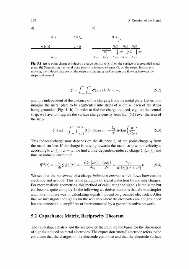
158 5 Creation of the Signal
0
q
σ (x,y)
0
q
0 000
Q1(t) Q2(t) Q3(t)
v
w I1(t) I2(t) I3(t)
a) b)
z = zo
z = 0
Fig. 5.1 (a) A point charge q induces a charge density σ(x,y) on the surface of a grounded metalplate. (b) Segmenting the metal plate results in induced charges Qn on the strips. In case q ismoving, the induced charges on the strips are changing and currents are flowing between thestrips and ground
Q =∫ ∞
−∞
∫ ∞
−∞σ(x,y)dxdy = −q, (5.2)
and it is independent of the distance of the charge q from the metal plate. Let us nowimagine the metal plate to be segmented into strips of width w, each of the stripsbeing grounded (Fig. 5.1b). In order to find the charge induced, e.g., on the centralstrip, we have to integrate the surface charge density from Eq. (5.1) over the area ofthe strip:
Q1(z0) =∫ ∞
−∞
∫ w/2
−w/2σ(x,y)dxdy = −2q
πarctan
(w
2z0
). (5.3)
This induced charge now depends on the distance z0 of the point charge q fromthe metal surface. If the charge is moving towards the metal strip with a velocity v
according to z0(t) = z0−vt, we find a time-dependent-induced charge Q1[z0(t)] andthus an induced current of
Iind1 (t) = − d
dtQ1[z0(t)] = −∂Q1[z0(t)]
∂ z0
dz0(t)dt
=4qw
π[4z0(t)2 +w2]v. (5.4)
We see that the movement of a charge induces a current which flows between theelectrode and ground. This is the principle of signal induction by moving charges.For more realistic geometries, this method of calculating the signals is the same butcan become quite complex. In the following we derive theorems that allow a simplerand more intuitive way of calculating signals induced on grounded electrodes. Afterthat we investigate the signals for the scenario where the electrodes are not groundedbut are connected to amplifiers or interconnected by a general reactive network.
5.2 Capacitance Matrix, Reciprocity Theorem
The capacitance matrix and the reciprocity theorem are the bases for the discussionof signals induced on metal electrodes. The expression ‘metal’ electrode refers to thecondition that the charges on the electrode can move and that the electrode surface

5.2 Capacitance Matrix, Reciprocity Theorem 159
is therefore an equipotential one. Setting a set of N metal electrodes to voltagesVn defines the potential φ(x) and the resulting electric field E(x) = −∇φ(x) inthe chamber volume. The potential is uniquely defined by the conditions that φ(x)satisfies the Laplace equation and that φ(x) = Vn on the electrode surfaces.
Figure 5.2a shows a set of three metal electrodes. The voltages Vn and chargesQn on the electrodes are related by the capacitance matrix of the electrode system[JAC 75]:
Qn =N
∑m=1
cnmVm. (5.5)
The capacitance matrix is defined by the electrode geometry, and for the capacitancematrix elements cnm, the following relations hold:
cnm = cmn, cnm ≤ 0 for n �= m, cnn ≥ 0,N
∑m=1
cnm ≥ 0 . (5.6)
These relations are a direct consequence of Green’s second theorem and the factthat the potential has to satisfy the Laplace equation. A set of different voltagesV n is related to a set of different charges Qn by the same capacitance matrix Qn =∑cnmV m, so by inverting this relation and multiplying it by Eq. (5.5) we find
N
∑n=1
QnV n =N
∑n=1
QnVn . (5.7)
This relation is called is called the reciprocity theorem and we use it frequently inthe following discussions. Another important relation concerns the sum of all thecharges of an electrode system. Figure 5.2b shows an electrode surrounding threeelectrodes. We apply Gauss’ law to the volume between the electrodes, which tellsus that the sum of all charges within this volume is equal to ε0 times the integral ofE(x) over the surface surrounding it. Because ε0
∫E(x)dA over a metal electrode
is equal to the charge on this electrode, we find that the sum of all charges on the
V1 Q1 V2 Q2
V3 Q3
V4 Q4
q2q1
b)
V1 Q1 V2 Q2
V3 Q3
a)
Fig. 5.2 (a) The voltages and charges in a system of electrodes are related by the capacitancematrix cnm. (b) A set of metal electrodes where one electrode encloses the others. The sum of allcharges Qn on the electrodes is equal to the sum of all charges qn in the volume between theelectrodes

160 5 Creation of the Signal
metal electrodes is equal to the sum of all charges in the volume between the elec-trodes! In the case where there are no charges in the volume between the electrodes,the sum of the charges Qn on the electrodes must be zero for any set of voltages Vn
applied to them. Thus for the capacitance matrix we find the relation
∑n
Qn = 0 → ∑n
∑m
cnmVm = 0 → ∑n
cnm = 0, (5.8)
which means that for a set of electrodes that is enclosed by one of them, the sum ofall columns (rows) of the capacitance matrix is equal to zero.
To conclude this section we note that the capacitance matrix elements cnm aredifferent from the more familiar capacitances Cnm that we know from electric circuitdiagrams. The Cnm are related to the voltage difference between circuit nodes, andwe show later that the cnm and Cnm are related by
Cnn =N
∑m=1
cnm, Cnm = −cnm if n �= m . (5.9)
5.3 Signals Induced on Grounded Electrodes, Ramo’s Theorem
We consider a set of three grounded electrodes in the presence of a point chargeQ0 = q at position x as shown in Fig. 5.3a. We assume the point charge Q0 to besitting on an (infinitely small) metal electrode, so we have a system of four metalelectrodes. For this setup we have V1 =V2 =V3 = 0 and we want to know the chargesQ1,Q2,Q3 induced by the presence of charge Q0 = q. Equation (5.7) reads
qV 0 +Q1V 1 +Q2V 2 +Q3V 3 = Q0V0 . (5.10)
Choosing another electrostatic state (Fig. 5.3b), where we remove the charge q fromthe small electrode (Q0 = 0), we set electrode 1 to voltage Vw (V 1 = Vw) whilekeeping the other electrodes grounded (V 2 = V 3 = 0), the above relation becomes
Q1
V1 = 0
Q2
Q3
V2 = 0
V3 = 0
Q0 = qV0
x
0
0
0
Q1
V1 = Vw
Q2
Q3
V2 = 0
V3 = 0
Q0 = 0 V0 = ψ1(x)
0
0
(a) (b)
Fig. 5.3 (a) The point charge q induces charges Qn on the grounded electrodes. (b) Another set ofvoltages and charges which defines the ‘weighting potential’ of the first electrode

5.4 Total Induced Charge and Sum of Induced Signals 161
Fig. 5.4 In the case wherethe charge q is moving thereare currents flowing betweenthe electrodes and ground.The definition of I = −dQ/dtindicates that the positivecurrent points away from theelectrode
Q1(t)
qx(t)
0
0
0
I1(t) I2(t)
I3(t)
Q2(t)
Q3(t)
qV 0 +Q1Vw = 0 → Q1 = −qV 0
Vw. (5.11)
V 0 is the potential of the uncharged small electrode for the second electrostatic state,and since an infinitely small uncharged electrode is equal to having no electrode, V 0
is the potential at point x when the point charge q is removed, electrode 1 is put topotential Vw, and electrodes 2 and 3 are grounded. We call V 0 = ψ1(x) the weightingpotential of electrode 1, and the induced charge Q1 is given by
Q1 = − qVw
ψ1(x) . (5.12)
In the case where the point charge q is moving along a trajectory x(t), as shownin Fig. 5.4, we find a time-dependent-induced charge on electrode n and therefore acurrent of
Iindn (t) = −dQn(t)
dt=
qVw
∇ψn[x(t)]dx(t)
dt= − q
VwEn[x(t)]v(t). (5.13)
We call En(x) = −∇ψn(x) the weighting field of electrode n, which is Ramo’stheorem [RAM 39]:
The current induced on a grounded electrode by a point charge q moving alonga trajectory x(t) is Iind
n (t) = −q/Vw En[x(t)]v(t), where En(x) is the electric fieldin the case where the charge q is removed, electrode n is set to voltage Vw, and allother electrodes are grounded.
It must be noted that the sign of the induced current is given not only by the signof the charge but also by the orientation of the particle velocity vector with respectto the direction of the weighting field. The trajectory x(t) is determined by the ‘real’electric and magnetic fields in the detector together with the drift properties of theelectrons and ions in the detector gas.
5.4 Total Induced Charge and Sum of Induced Signals
If the charge q is moving along a trajectory x(t) from position x0 = x(t0) to positionx1 = x(t1), the total amount of charge Qind
n that flows between electrode n andground is given by
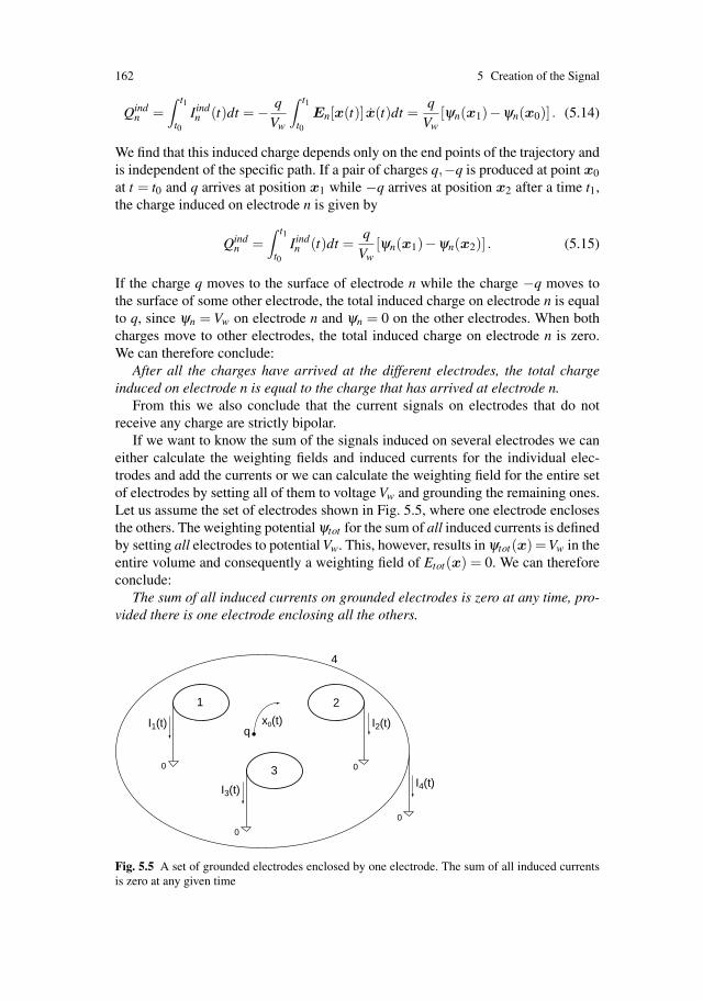
162 5 Creation of the Signal
Qindn =
∫ t1
t0Iindn (t)dt = − q
Vw
∫ t1
t0En[x(t)] x(t)dt =
qVw
[ψn(x1)−ψn(x0)] . (5.14)
We find that this induced charge depends only on the end points of the trajectory andis independent of the specific path. If a pair of charges q,−q is produced at point x0
at t = t0 and q arrives at position x1 while −q arrives at position x2 after a time t1,the charge induced on electrode n is given by
Qindn =
∫ t1
t0Iindn (t)dt =
qVw
[ψn(x1)−ψn(x2)] . (5.15)
If the charge q moves to the surface of electrode n while the charge −q moves tothe surface of some other electrode, the total induced charge on electrode n is equalto q, since ψn = Vw on electrode n and ψn = 0 on the other electrodes. When bothcharges move to other electrodes, the total induced charge on electrode n is zero.We can therefore conclude:
After all the charges have arrived at the different electrodes, the total chargeinduced on electrode n is equal to the charge that has arrived at electrode n.
From this we also conclude that the current signals on electrodes that do notreceive any charge are strictly bipolar.
If we want to know the sum of the signals induced on several electrodes we caneither calculate the weighting fields and induced currents for the individual elec-trodes and add the currents or we can calculate the weighting field for the entire setof electrodes by setting all of them to voltage Vw and grounding the remaining ones.Let us assume the set of electrodes shown in Fig. 5.5, where one electrode enclosesthe others. The weighting potential ψtot for the sum of all induced currents is definedby setting all electrodes to potential Vw. This, however, results in ψtot(x) =Vw in theentire volume and consequently a weighting field of Etot(x) = 0. We can thereforeconclude:
The sum of all induced currents on grounded electrodes is zero at any time, pro-vided there is one electrode enclosing all the others.
1
qx0(t)
0
0
0
I1(t) I2(t)
I3(t)
2
3
0
4
I4(t)
Fig. 5.5 A set of grounded electrodes enclosed by one electrode. The sum of all induced currentsis zero at any given time

5.5 Induced Signals in a Drift Tube 163
5.5 Induced Signals in a Drift Tube
As an example we calculate the induced signal in a drift tube with (cathode) radius band wire radius a (Fig. 5.6). The tube is set to potential −U and the wire is grounded.This results in an electric field of E(r) = U/(r ln(b/a)), as calculated in Sect. 3.1.1.We assume a single primary electron-ion pair in the gas volume. The electron movesto the wire and the ion moves to the tube wall. Close to the wire the electron starts anavalanche creating Ntot electrons and ions. The Ntot electrons of charge −e0 move tothe wire surface within a time much less than a nanosecond. The Ntot ions of charge+e0 move away from the wire, but much more slowly, arriving at the tube wall aftera time typically several hundreds of microseconds. As a first step we simply assumethat the Ntot electrons are created at the wire surface and so do not move, while theNtot ions move from the wire surface to the tube wall. The velocity of the ions isgiven by the mobility μ as v = μE, so with the condition that r(t = 0) = a we findthe ion trajectory to be
dr(t)dt
= μU
r(t) ln(b/a)→ r(t) = a
√1+
tt0
t0 =a2 ln(b/a)
2μU(5.16)
The characteristic time t0 is typically one or a few nanoseconds. It takes very muchlonger for the ions to arrive at the tube wall r = b; this maximum travel time istmax = t0[(b/a)2 −1], typically four to six orders of magnitude larger than t0, in thehundred microsecond range.
The weighting potential ψ1 and weighting field E1 of the wire are defined bysetting the wire to potential Vw and grounding the tube, which results in
ψ1(r) = −Vw ln(r/b)ln(b/a)
E1(r) =Vw
r ln(b/a)(5.17)
According to Eq. (5.13), the current induced on the wire by the movement of theNtot ions is given by
Iind1 (t) = −Ntote0
VwE1[r(t)] r(t) = − Ntote0
2 ln(b/a)1
t + t0. (5.18)
The wire signal is negative and has a hyperbolic form with a characteristic timeconstant t0, which in practical cases will be a few nanoseconds. The induced chargeat time t is given by
Fig. 5.6 Ions moving fromthe wire surface to the tubewall induce a current signalon the grounded wire 0
–U
I(t)

164 5 Creation of the Signal
Qind1 (t) =
∫ t
0Iind1 (t ′)dt ′ = − Ntote0
2 ln(b/a)ln
(1+
tt0
). (5.19)
Once the ions have arrived at the tube wall the induced charge on the wire isQind
1 (tmax) = −Ntote0, which agrees with the statement about the total inducedcharge from the previous section. The current induced on the tube (‘the cathode’) isIind2 (t) = −Iind
1 (t) since the tube completely encloses the wire and thus the sum ofthe two signals must be zero at any time.
As an illustration, in Fig. 5.7 we plot the time development of a current pulsedescribed by Eqs. (5.18) and (5.19) using typical parameters for a,b, and t0. Oneobserves the extremely sharp onset and the extremely long tail characteristic of suchpulses.
In a second step we refine the picture by involving the radial extent of theavalanche, the electron movement, and the field dependence of the ion mobility.We use the model from Sect. 4.4.1, where the Townsend coefficient was taken to beproportional to the electric field (α = (ln2/ΔV )E) and the first multiplication startsat a minimum field Emin. With Emin = U/(rmin ln(b/a)), the number of electronspresent at distance r is given by
N(r) = exp
(∫ rmin
rα(r)dr
)=( rmin
r
) U ln2ΔV ln(b/a) (5.20)
The total number of avalanche electrons (the gain) is Ntot = N(a). The numberof electrons created between r and r + dr is n(r)dr = (dN/dr)dr, so the centre ofgravity rcog of the electron avalanche is given by
rcog =1
Ntot
∫ rmin
ar n(r)dr = a(1+ ε) ε =
ΔV ln(b/a)U ln2
(5.21)
Typical operating voltages U of ≈ 2 kV, ΔV values of ≈ 20V , and ln(b/a) valuesof ≈ 10 result in a value for ε of the order of 0.1. With traditional wire radii ofa = 10−30 μm we find that the centre of gravity of the electron avalanche is only afew micrometers above the wire surface.
With such a small distance to travel to their destination, the wire surface, theelectrons can only make a small contribution to the total signal charge. The latter
Fig. 5.7 Current signalaccording to (5.18) ( fullline, left-hand scale) fort0 = 1.25 ns, b/a = 500, andq = 106 elementary charges.Time integral (5.19) of thispulse as a percentage of thetotal (broken line, right-handscale)
5.6 Signals Induced on Electrodes Connected with Impedance Elements 165
one is given by Qindtot = −e0Ntot once all the electrons and ions have arrived on
their respective electrodes (see the previous section). The signal from the electronsmay be calculated using Eq. (5.14), which tells us that a single electron movingfrom distance r to the wire surface induces a charge of −(e0/vw)(ψ1(a)−ψ1(r)) =−e0 ln(r/a)/ ln(b/a). Thus, assuming that all the electrons are moving from rcog tothe wire surface, the fraction of charge induced by the avalanche electrons is givenby
Qinde
Qindtot
=ln(rcog/a)ln(b/a)
≈ ΔVU ln2
. (5.22)
For typical values of U and ΔV discussed above, the fraction of charge inducedby the movement of the electrons amounts to 1 or 2% of the total induced charge.Since the electrons arrive at the wire within a time much shorter than 1 ns, for allpractical purposes we can assume the electron component of the signal to be a deltacurrent Iind
e (t) = Qinde δ (t). The ions move from their point of creation to the tube
wall, and we assume here that they all start from rcog. In the high electric fields of103–104V/(cm Torr) in the vicinity of the wire, the ion velocity is not proportionalto E but rather is related to the field by v = κ
√E (Sect. 2.2.2). Thus, for the early
part of the ion trajectory we have
dr(t)dt
= κ
√U
r(t) ln(b/a)→ r(t) = a(1+ ε)
√1+
tt1
t1 =2
3κ
√ln(b/a)
Ua3(1+ ε)3. (5.23)
In practice, t1 is a small factor (say two or three times) larger than t0. It is remarkablethat the functional dependence on t is the same as the one of the simplified case ofEq. (5.16). The refinements have only changed the numerical values of t0 and a, sothe signal again assumes a hyperbolic form with a characteristic time constant t1.The sharp onset and the long tail remain as shown in Fig. 5.7.
Since the electric field in the vicinity of the wire of any wire chamber has theform 1/r, the universal shape of the induced current signal Iind
1 (t) Eq. (5.18) is validfor wire signals of all wire chamber geometries.
5.6 Signals Induced on Electrodes Connectedwith Impedance Elements
In this section we calculate the signals induced by moving charges on electrodesconnected with arbitrary impedance elements. Before doing this, however, we firstinvestigate the circuit shown in Fig. 5.8, where external current sources In areimpressed on nodes which are connected to impedances Znm. These impedancesrepresent linear ‘physical’ objects such as resistors, capacitors, and amplifiers. Inthe Laplace domain (see Chap. 6), the current Inm flowing from node n to node m

166 5 Creation of the Signal
Fig. 5.8 Circuit diagramrepresenting three nodesconnected to each other andground through impedancesZnm. The In(t) representexternal currents impressedon the nodes, and theVn(t) represent the resultingvoltages
V1(t)Z12
Z23
0
Z2Z11
0
Z13
0
Z33
V2(t)
V3(t)
I1(t) I2(t)
I3(t)
through Znm and the current Inn flowing between node n and ground through Znn aredefined by
Inm(s) = [Vn(s)−Vm(s)]/Znm(s) and Inn(s) = Vn(s)/Znn(s) . (5.24)
On every node, the sum of all currents must be zero, which gives
In − Inn − ∑m�=n
Inm = 0 → In = ∑m
ynmVm, (5.25)
where we have defined the admittance matrix ynm of the circuit as
ynn = ∑m
1Znm
ynm = − 1Znm
n �= m. (5.26)
The voltages on the nodes, resulting from the impressed currents, are thereforegiven by
Vn(s) = ∑m
znm(s)Im(s) znm(s) = y−1nm(s). (5.27)
The matrix znm is the inverse of the admittance matrix and is called the impedancematrix of the circuit.
Up to this point we have understood that there is a linear relationship [Eq. (5.25)or Eq. (5.27)] between the currents In(t) impressed on the nodes of the network(Fig. 5.8) and the resulting potentials Vn(t) on the nodes. What we finally wantto determine are the potentials V ind
n (t) induced by a moving charge q between theelectrodes that are part of a network as shown in Fig. 5.9a. In the following wewill find that these voltages are calculated by adding the mutual electrode capaci-tances to the network from Fig. 5.8 and placing the currents that would be inducedon grounded electrodes as impressed currents to this circuit (Fig. 5.9b). The driftof charges in gases is slow enough to allow the use of the quasi-electrostatic cal-culation, meaning that Eq. (5.5) and the reciprocity theorem (5.7) are also valid fortime-dependent charges Qn(t) and voltages Vn(t) at every time t. Following the pro-cedure of Sect. 5.3, we use a second electrostatic state, where Q0(t) = 0, V 1(t) =Vw
and V 2(t) = V 3(t) = 0, which gives

5.6 Signals Induced on Electrodes Connected with Impedance Elements 167
00
0
V1ind(t)
qx(t)
0
0
0
Z11
Z33
Z22
Z12
Z13
Z23
a) b)
V2ind(t)
V3ind(t)
V1ind(t) V2
ind(t)
V3ind(t)
I1ind(t) I2
ind(t)
I3ind(t)
Fig. 5.9 (a) The point charge q induces voltages on the electrodes that are connected withimpedance elements. (b) These induced voltages are calculated by adding the mutualelectrode-electrode capacitances Cnm to the equivalent circuit and placing the currents, induced onthe grounded electrodes, as impressed current sources on the nodes
qψ1(x)+Q1 Vw = Q1V ind1 +Q2V ind
2 +Q3V ind3 . (5.28)
The charges Qn and voltages V n are related by the capacitance matrix of thethree-electrode system giving Qn = c1nVw. Writing the same relations for the otherelectrodes results in
Qn = − qVw
ψn(x)+∑m
cnmV indm ,s (5.29)
where Qn, V indn , and ψn are the charge, voltage, and weighting potential of electrode
n. If the point charge q moves along the trajectory x(t) we find time-dependentcharges Qn on the electrodes, and their rate of change is
dQn
dt= −Iind
n (t)+∑m
cnmdV ind
m
dt. (5.30)
The Iindn (t) are the currents from Eq. (5.13) induced on the electrodes in the case
where they are grounded. The charges Qn can only change due to currents flowingbetween the electrodes, i.e., dQn/dt = ∑m Inm + Inn. These currents in turn are givenby the potential differences and connecting impedances, as defined in Eq. (5.24). Inthe Laplace domain we therefore have
∑m
(V indm −V ind
n )Znm
+V ind
n
Znn= −Iind
n +∑m
scnmV indm → (5.31)
Iindn = ∑
m(scnm + ynm)V ind
m or V indn = ∑
m(sc+ y)−1
nmIindm , (5.32)
where the admittance matrix ynm is defined in Eq. (5.26). The following is our finalresult:

168 5 Creation of the Signal
The voltages V indn (t) induced by a moving charge on electrodes connected to
impedances Znm(s) are determined by first using Ramo’s theorem to calculate thecurrents induced on the grounded electrodes and placing them as ideal currentsources on an equivalent circuit diagram with admittance matrix scnm + ynm(s)(Fig. 5.9b).
The additional admittance matrix elements scnm are due to the mutual capaci-tance between the electrodes. Inverting the relation (5.26) for yc
nm = scnm, we seethat the impedances corresponding to cnm are given by
Zcnm =
1sCnm
with Cnn = ∑m
cnm Cnm = −cnm n �= m (5.33)
The Cnm are the electrode capacitances, which must be distinguished from the capac-itance matrix cnm in the same way that the impedances Znm must be distinguishedfrom the impedance matrix znm. The equivalent circuit for Eq. (5.32) is shown inFig. 5.9b. To calculate the induced voltages we compute the currents induced ongrounded electrodes with Ramo’s theorem and perform the next step of the calcula-tion analytically or, e.g., with an analog circuit simulation program.
For the completion of our task we still have to specify the actual trajectory ofthe moving charge, and we must find the numerical values of the capacitance matrixelements. For this, the weighting fields known from Eq. (5.13) turn out to be use-ful because they have a simple relation to the capacitance matrix as well as to thetrajectory-defining field E(x). If metal electrodes are set to voltages Vn, the poten-tial ψ(x) is uniquely defined by the requirements that it fulfils the Laplace equationin the volume between the electrodes and that ψ(x) = Vn on the electrode surfaces.The potential
ψ(x) = ∑n
Vn
Vwψn(x) (5.34)
satisfies these conditions because the weighting potentials ψn are equal to Vw onelectrode n and zero on the other electrodes, and since such a solution is unique itis the general solution of this problem. From this we immediately obtain the fieldE(x) as a linear superposition of the weighting fields:
E(x) = ∑n
Vn
VwEn(x) . (5.35)
The surface charge density on a metal electrode is related to the electric field onthe surface by σ = ε0|E|. The total charge on electrode n is therefore defined by theintegral over the electrode surface An
Qn = ε0
∮An
E(x)dA = ∑m
Vm
Vw
∮An
Em(x)dA = ∑m
cnmVm. (5.36)
As a result, the capacitance matrix elements are calculated to be
cnm =ε0
Vw
∮An
Em(x)dA . (5.37)

5.6 Signals Induced on Electrodes Connected with Impedance Elements 169
Knowing the weighting fields En(x) is therefore sufficient to calculate the chambersignals in four steps:
1. Using Eq. (5.35) we find the ‘real’ electric field in the chamber which determinesthe particle trajectories.
2. The induced currents on grounded electrodes follow from Ramo’s theorem[Eq. (5.13)].
3. The capacitance matrix cnm and capacitances Cnm are calculated from Eqs. (5.37)and (5.33).
4. These capacitance elements are added to the equivalent circuit and the inducedcurrents are impressed on the nodes as ideal current sources.
The calculation of the weighting fields and capacitance matrix is performedanalytically or with dedicated computer programs. The final step of placing the cur-rents on the equivalent circuit diagram is usually done by analog circuit simulationprograms.
5.6.1 Application to a Drift Tube and its Circuitry
We now illustrate the above procedure by applying it to the drift tube shown inFig. 5.10a. For our example we use values of l = 100cm, tube radius b = 1.5cm,and wire radius a = 25 μm.
We first have to calculate the electric field in the detector and determine theion trajectories, as done in Eq. (5.16). Next we calculate the weighting fields andthe induced current signals using Ramo’s theorem, which was done in Eq. (5.18).In a third step we calculate the capacitance matrix of the tube using Eq. (5.37).Electrode 1 (the wire) has an area of A1 = 2aπlr and electrode 2 (tube) has anarea of A2 = −2bπlr. With the weighting fields E1 = Vw/r ln(b/a)r (wire) andE2 = −Vw/r ln(b/a)r (tube) we find
c11 = c22 = −c12 = −c21 =2πε0l
ln(b/a). (5.38)
0
+U
Rin
RL
0
C
a) 0
+U
Rin
RL
0
C
b)
C12
I1ind(t)
–I1ind(t)
Wire
Tube
l
IA(t)
Fig. 5.10 (a) Typical setup for a drift tube. The wire is set to voltage U and is decoupled from theamplifier input by a capacitor C. (b) The signals in the presence of the reactive elements arecalculated by placing the currents Iind
n (t), induced on the grounded electrodes, as ideal currentsources on the equivalent circuit
170 5 Creation of the Signal
The capacitances, calculated by Eq. (5.33), are therefore
C11 = C22 = 0 C12 = C21 =2πε0l
ln(b/a). (5.39)
For the chosen parameters we find C12 = 20 pF. In the final step we impress theinduced currents as ideal current sources on the equivalent circuit of the tube asshown in Fig. 5.10b. The wire is read out by an amplifier with input resistanceRin, which we choose to be 50Ω . In the equivalent circuit, the wire and the tubehave become pointlike nodes. This is only admissible if the tube is ‘electricallyshort’, i.e., if the shortest wavelength λ = c/ f0 processed by the readout electronicswith bandwidth limit f0 is large compared to the tube length l. For the assumedparameters this translates into f0 300MHz. We use a value of 1.6 MHz in thefollowing. In a case where l is not much smaller than c/ f0 we would have to considerthe tube to be a transmission line. In practical applications it is not convenient to setthe tube to negative high voltage −U , as shown in Fig. 5.6, but rather to ground thetube and set the wire to positive voltage U . The signal −Iind
1 induced on the tube canbe neglected because the current is ‘leaving’ to the ground node and is not enteringthe amplifier.
Choice of the circuit parameters. The capacitor C decoupling the amplifierfrom the potential U must be large compared to C12 so that the current signal goesinto the amplifier instead of flowing into C12. But it must not be so large that theenergy E = CU2/2 it stores would destroy the amplifier in the case of a spark. Letus take the typical value of 1 nF for C.
The resistor RL connects the wire to the voltage supply. It must be large in com-parison to the impedance of C and Rin in series so that only a small fraction ofthe signal is lost into the power supply. If we want 99% of the bandwidth to findthis impedance sufficiently small, we may evaluate it at 1% of the bandwidth limitleaving a value of
RL >1
2π f0 ×0.01+Rin ≈ 104Ω (5.40)
in our example. In addition, this resistor is a source of thermal current noise whichis proportional to 1/
√RL, so in this respect as well one chooses the resistor as large
as possible. The upper limit for RL is defined by the maximum voltage drop thatone allows for a given chamber current. With a primary ionization of, e.g., 125 elec-trons and a gas gain of 5× 10⁵ at a rate of 100 kHz, we find a chamber currentof 1 μA, which leads to a tolerable voltage drop of 1 V for an RL value of 1MΩ .Values for RL of 100 kΩ to several MΩ are typical; let us make RL = 1MΩ fordefiniteness.
The relation between the induced current Iind1 and amplifier input current IA can
be determined by evaluating the equivalent circuit diagram in Fig. 5.10b. Using themethods of Chap. 6 we change to the Laplace domain and find
IA(s) =sRLC
1+ s(RLC +RinC +RLC12)+ s2RinC12RLCIind1 (s) . (5.41)
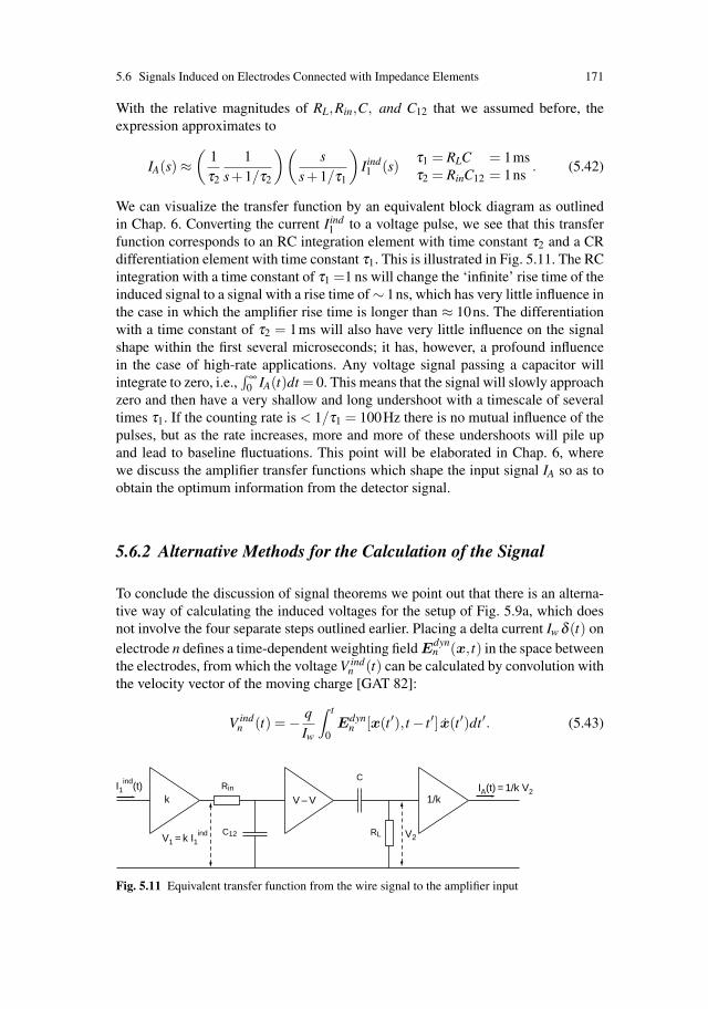
5.6 Signals Induced on Electrodes Connected with Impedance Elements 171
With the relative magnitudes of RL,Rin,C, and C12 that we assumed before, theexpression approximates to
IA(s) ≈(
1τ2
1s+1/τ2
)(s
s+1/τ1
)Iind1 (s)
τ1 = RLC = 1msτ2 = RinC12 = 1ns
. (5.42)
We can visualize the transfer function by an equivalent block diagram as outlinedin Chap. 6. Converting the current Iind
1 to a voltage pulse, we see that this transferfunction corresponds to an RC integration element with time constant τ2 and a CRdifferentiation element with time constant τ1. This is illustrated in Fig. 5.11. The RCintegration with a time constant of τ1 =1 ns will change the ‘infinite’ rise time of theinduced signal to a signal with a rise time of ∼ 1ns, which has very little influence inthe case in which the amplifier rise time is longer than ≈ 10ns. The differentiationwith a time constant of τ2 = 1ms will also have very little influence on the signalshape within the first several microseconds; it has, however, a profound influencein the case of high-rate applications. Any voltage signal passing a capacitor willintegrate to zero, i.e.,
∫ ∞0 IA(t)dt = 0. This means that the signal will slowly approach
zero and then have a very shallow and long undershoot with a timescale of severaltimes τ1. If the counting rate is < 1/τ1 = 100Hz there is no mutual influence of thepulses, but as the rate increases, more and more of these undershoots will pile upand lead to baseline fluctuations. This point will be elaborated in Chap. 6, wherewe discuss the amplifier transfer functions which shape the input signal IA so as toobtain the optimum information from the detector signal.
5.6.2 Alternative Methods for the Calculation of the Signal
To conclude the discussion of signal theorems we point out that there is an alterna-tive way of calculating the induced voltages for the setup of Fig. 5.9a, which doesnot involve the four separate steps outlined earlier. Placing a delta current Iw δ (t) onelectrode n defines a time-dependent weighting field Edyn
n (x, t) in the space betweenthe electrodes, from which the voltage V ind
n (t) can be calculated by convolution withthe velocity vector of the moving charge [GAT 82]:
V indn (t) = − q
Iw
∫ t
0Edyn
n [x(t ′), t − t ′] x(t ′)dt ′. (5.43)
k V – V 1/kRin
RLC12
CI1
ind(t) IA(t) = 1/k V2
V1 = k I1
ind V2
Fig. 5.11 Equivalent transfer function from the wire signal to the amplifier input

172 5 Creation of the Signal
This theorem can be useful when one studies a detector geometry with a simulationprogram that allows the transient analysis of time-dependent electric fields.
There are detectors with electrodes that have only a finite conductivity, such asresistive plate chambers (RPCs) [SAN 80] or undepleted silicon detectors. In suchcases, which do not normally occur in wire chambers, the theorems discussed in thischapter are not directly applicable, but have to be generalized. An extension of thetheorems of signal generation including resistive electrodes as well as dissipativedielectrics has been published elsewhere [RIE 04].
5.7 Signals Induced in Multiwire Chambers
A classical multiwire chamber consists of a plane of anode wires situated betweentwo parallel cathode planes. Often one of the cathode planes is subdivided intostrips orthogonal to the wires; then the avalanches can be localized in two dimen-sions by reading out the electrical signals from the wires and the strips [GAT 79].Such a geometry is depicted further on in Fig. 5.14. In the following we discuss themain characteristics of the wire and cathode signals using the method outlined inSect. 5.1–5.4.
5.7.1 Signals Induced on Wires
The wire radii, typically 10–30 μm, are small compared to the distance betweenthe wires and the distance between the wire and the cathode of typically a fewmillimetres. This fact gives rise to a coaxial electric field close to the wires, as weshow in the following. Setting the wires to potentials Un results in charges qn on thewires, which are determined by the capacitance matrix through qn = ∑N
m=1 cnm Um.We combine the two cathode planes into electrode 1 and label the individual wiresas electrodes 2, 3, 4, etc. (cf. Fig. 5.12). We assume the wires to be infinitely long,so cnm and qn are the capacitance matrix and charge per unit of wire length. Theelectric field at a distance r from a line charge q is given by
E(r) =q
2πε0 rr, (5.44)
cathode plane
anode wires
cathode plane
electrode ′1′
′2′ ′3′ ′4′
′1′
Fig. 5.12 Electrode arrangement for which the induced currents are calculated in (5.48) to (5.51).Wire ‘2’ carries the avalanche
5.7 Signals Induced in Multiwire Chambers 173
so at a point with distance r1 and r2 to two wires carrying charge q1 and q2, theelectric field is E = 1/(2πε0)([q1/r1]r1 + [q2/r2]r2). In the vicinity of a wire,meaning that r1 r2, the field is dominated by the charge on this wire as longas the charges q1 and q2 are of similar magnitude. We can conclude that the elec-tric field at distance r from wire n is approximately coaxial, and its magnitudegiven by
E(r) =qn
2πε0 r=
12πε0 r
(N
∑m=1
cnmUm
)(5.45)
as long as r is small compared to the distance between the chamber electrodes. Un-der these circumstances, the trajectory of the avalanche ions is just the same as theone in the drift tube [Eq. (5.16)], and we have
r(t) = a√
1+ t/t01t0
=μ
a2πε0
(N
∑m=1
cnmUm
). (5.46)
It is interesting to note that it is the bandwidth of the electronics which decideswhether the coaxial approximation (5.45) is adequate. Imagine a fast amplifier (largebandwidth) for signals only 50 ns long: with typical values of 1 ns for t0 and 15 μmfor the wire radius a, the ions have travelled only a few percent of a typical wire pitchof 1.5 or 2 mm, namely 0.1 mm in 50 ns – the coaxial approximation is probablygood enough in most circumstances. On the other hand, imagine a slower amplifier(smaller bandwidth) for signals 1 μs long: with the same typical values the ionshave already travelled a significant fraction of the typical wire pitch, namely 0.5 mmin 1 μs – the coaxial approximation is probably not good in many circumstances,and the signal shape begins to depend on the angular distribution of avalanche ionsaround the wire.
For the time being we wish to stay in the coaxial approximation (5.45) in orderto compute the signals on the various wires. We consider the situation with a planeof anode wires, all on the same potential, between two cathode plates, as depictedin Fig. 5.12.
Knowing the ion trajectory r(t) we need to calculate the weighting fields ofthe wires in order to find the induced current signals. The weighting field of theavalanche wire (electrode ‘2’), where the avalanche takes place, is found by settingthe wire to voltage Vw and grounding all other wires and electrodes. This results inthe charge q2 = c22Vw on this wire, and the magnitude of the weighting field in thecoaxial approximation is
E2(r) =c22Vw
2πε0 r. (5.47)
The current induced by Ntot ions of charge e0, moving away from the wire surface,is therefore
I2(t) = −Ntote0
VwE2[r(t)]
drdt
= −Ntote0
4πε0
c22
t + t0. (5.48)
The signal on the avalanche wire is negative because c22 > 0 [cf. Eq. (5.6)].

174 5 Creation of the Signal
The weighting field of the closest neighbour (electrode ‘3’) is given by settingwire ‘3’ to potential Vw and grounding all other wires. This results in a charge ofq3 = c23Vw on the avalanche wire and the signal on wire ‘3’ is therefore
I3(t) = −Ntote0
4πε0
c23
t + t0. (5.49)
The ‘cross-induced’ signal has the same shape as the signal on the avalanche wireand because c2n < 0,n �= 2, it is positive. The other wires have the same signalpolarity and shape, with relative amplitudes c24,c25, etc. We can express the relativesignal amplitudes by the more familiar capacitances Cnm and find
In(t)I1(t)
=c2n
c22= − C1n
∑Nm=1 C2m
. (5.50)
The amplitude of the ‘cross-induced’ signal from the avalanche wire to wire n istherefore given by the mutual capacitance between the avalanche wire and wire ndivided by the sum of all mutual capacitances of the avalanche wire to the otherelectrodes.
We have to note that the capacitive coupling between wires causes a signal ofthe same polarity on the neighbouring wires, which can be seen, e.g., by injecting awire signal with a pulse generator. During the early days of wire chamber develop-ment one feared that the resolution of multiwire chambers was limited owing to thiscapacitive coupling, which increases as the wire spacing is reduced. The oppositepolarity of the signal induced by the avalanche is, however, hiding this capacitivecrosstalk, which makes it ‘a simple matter to localize the wire which is the seed ofthe avalanche, whatever the distance between the wires’ [CHA 92].
The sum of all wire signals is given by
Iw(t) =N
∑n=2
In(t) = −Ntote0
4πε0
1t + t0
N
∑n=2
c1n = −Ntote0
4πε0
C12
t + t0. (5.51)
Here we have used the relation C12 = −c12 and the fact that the two cathodeplanes completely enclose the wires and the sum of all capacitance matrix elements∑N
m=1 cnm is zero. The sum of all wire signals thus has negative polarity. If all thewires are set to the same voltage U , the characteristic time constant t0 from Eq.(5.46) assumes the form
1t0
=μ
a2πε0
(U
N
∑m=2
cnm
)=
μU C12
a2πε0. (5.52)
For a comparison with the simple drift tube with wire radius a and tube radiusb, we remember that the wire signal and wire capacitance per unit length C′
12 werecalculated [Eqs. (5.16), (5.18), (5.39)] to be
I(t) = − Ntote0
2 ln(b/a)1
t + t0
1t0
=2μU
a2 ln(b/a)C′
12 =2πε0
ln(b/a). (5.53)
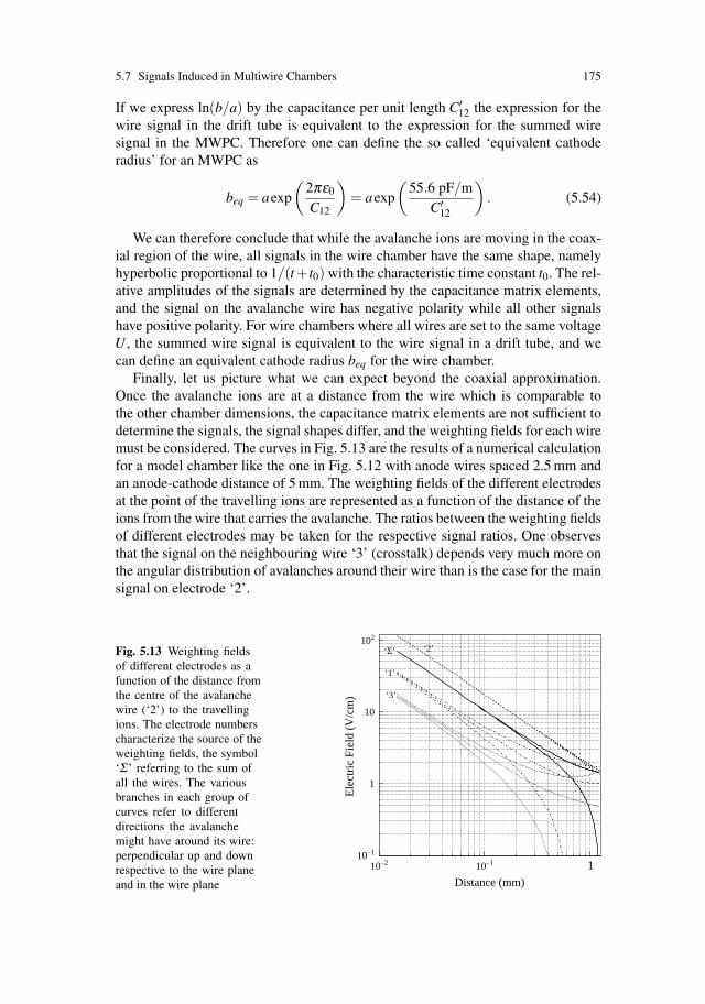
5.7 Signals Induced in Multiwire Chambers 175
If we express ln(b/a) by the capacitance per unit length C′12 the expression for the
wire signal in the drift tube is equivalent to the expression for the summed wiresignal in the MWPC. Therefore one can define the so called ‘equivalent cathoderadius’ for an MWPC as
beq = aexp
(2πε0
C12
)= aexp
(55.6 pF/m
C′12
). (5.54)
We can therefore conclude that while the avalanche ions are moving in the coax-ial region of the wire, all signals in the wire chamber have the same shape, namelyhyperbolic proportional to 1/(t +t0) with the characteristic time constant t0. The rel-ative amplitudes of the signals are determined by the capacitance matrix elements,and the signal on the avalanche wire has negative polarity while all other signalshave positive polarity. For wire chambers where all wires are set to the same voltageU , the summed wire signal is equivalent to the wire signal in a drift tube, and wecan define an equivalent cathode radius beq for the wire chamber.
Finally, let us picture what we can expect beyond the coaxial approximation.Once the avalanche ions are at a distance from the wire which is comparable tothe other chamber dimensions, the capacitance matrix elements are not sufficient todetermine the signals, the signal shapes differ, and the weighting fields for each wiremust be considered. The curves in Fig. 5.13 are the results of a numerical calculationfor a model chamber like the one in Fig. 5.12 with anode wires spaced 2.5 mm andan anode-cathode distance of 5 mm. The weighting fields of the different electrodesat the point of the travelling ions are represented as a function of the distance of theions from the wire that carries the avalanche. The ratios between the weighting fieldsof different electrodes may be taken for the respective signal ratios. One observesthat the signal on the neighbouring wire ‘3’ (crosstalk) depends very much more onthe angular distribution of avalanches around their wire than is the case for the mainsignal on electrode ‘2’.
Fig. 5.13 Weighting fieldsof different electrodes as afunction of the distance fromthe centre of the avalanchewire (‘2’) to the travellingions. The electrode numberscharacterize the source of theweighting fields, the symbol‘Σ ’ referring to the sum ofall the wires. The variousbranches in each group ofcurves refer to differentdirections the avalanchemight have around its wire:perpendicular up and downrespective to the wire planeand in the wire plane
10–1
1
10
102
10–2 10–1 1Distance (mm)
Ele
ctri
c Fi
eld
(V/c
m)
‘2’
‘1’
‘3’
‘Σ’

176 5 Creation of the Signal
5.7.2 Signals Induced on Cathode Strips and Pads
When the wires are enclosed by the two cathode planes, the sum of all chamber sig-nals is zero at any time and the cathode signal Ic(t) is equal to the negative summedwire signal −Iw(t). In our example, the cathodes are symmetrically placed withrespect to the wire plane, so the signal on a single cathode plane in the coaxialapproximation is
Ic1(t) =12
Ic(t) = −12
Iw(t) =12
Ntote0
4πε0
C12
t + t0. (5.55)
The avalanche can be localized in the direction perpendicular to the sense wire whensubdividing the cathode into separate strips or pads, as indicated in Fig. 5.14. Theweighting field of a cathode strip is calculated by setting the strip to potential Vw
while grounding all other strips and wires. This method is used in [MAT 84a] to ar-rive at the exact expression for the weighting field and induced signal. For practicalpurposes a few simplifications can be introduced [GAT 79][MAT 84b]. The signalon a cathode strip is determined by first calculating the signal on a strip of infinites-imal width, which is then integrated over the strip width w. This procedure definesa so-called cathode charge distribution Γ (λ ) through
dIc1(t,λ ) = Ic(t)Γ (λ )dλ∫ ∞
−∞Γ (λ )dλ =
12, (5.56)
where λ = x/h is the distance of the infinitesimal strip from the avalanche posi-tion. The distribution Γ (λ ) can be calculated by investigating the weighting fieldof an infinitesimal cathode strip. A single-parameter semi-empirical expression forΓ (λ ) was given by Gatti et al. [GAT 79] and discussed by Mathieson and Gordon[MAT 84b]:
Γ (λ ) = K11− tanh2 K2λ
1+K3 tanh2 K2λ. (5.57)
Here the parameters K1 and K2 are uniquely defined by K3, which depends on thechamber geometry as shown in Fig. 5.15:
Fig. 5.14 A row of wirescentred between two cathodeplanes. By segmenting thecathode into strips, theposition of the avalanchealong the wire direction canbe determined. The wire pitchs, the strip width w = 2a,and the distance h betweenanode and cathode planes areindicated
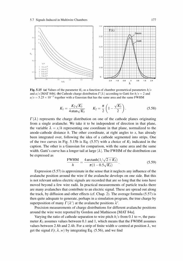
5.7 Signals Induced in Multiwire Chambers 177
Γ(λ)
λ
Gauss
Gatti
0
Fig. 5.15 (a) Values of the parameter K3 as a function of chamber geometrical parameters h/sand a/s [MAT 84b]. (b) Cathode charge distribution Γ (λ ) according to Gatti for h/s = 2 anda/s = 5.25×10⁻³ together with a Gaussian that has the same area and the same FWHM
K1 =K2
√K3
4atan√
K3K2 =
π2
(1−
√K3
2
). (5.58)
Γ (λ ) represents the charge distribution on one of the cathode planes originatingfrom a single avalanche. We take it to be independent of direction in that plane,the variable λ = x/h representing one coordinate in that plane, normalized to theanode-cathode distance h. The other coordinate, at right angles to x, has alreadybeen integrated over, following the idea of a cathode segmented into strips. Oneof the two curves in Fig. 5.15b is Eq. (5.57) with a choice of K3 indicated in thecaption. The other is a Gaussian for comparison, with the same area and the samewidth. Gatti’s curve has a longer tail at large |λ |. The FWHM of the distribution canbe expressed as
FWHMh
=4arctanh(1/
√2+K3)
π(1−0.5√
K3). (5.59)
Expression (5.57) is approximate in the sense that it neglects any influence of theavalanche position around the wire if the avalanche develops on one side. But thisis not relevant unless electric signals are recorded that are so long that the ions havemoved beyond a few wire radii. In practical measurements of particle tracks thereare many avalanches that contribute to an electric signal. These are spread out alongthe track, by diffusion and other effects (cf. Chap. 2). The average formula (5.57) isthen quite adequate to generate, perhaps in a simulation program, the true charge bysuperposition of many Γ (λ i) at the avalanche positions λ i.
Precision measurements of charge distributions for different avalanche positionsaround the wire were reported by Gordon and Mathieson [MAT 84a].
Varying the ratio of cathode separation to wire pitch h/s from 0.1 to ∞, the para-meter K3 assumes values between 0.1 and 1, which means that the FWHM assumesvalues between 2.8h and 2.4h. For a strip of finite width w centred at position λ , weget the signal I(t,λ ,w) by integrating Eq. (5.56), and we find

178 5 Creation of the Signal
I(t,λ ,w) =∫ λ+w/2
λ−w/2dIc1(t,λ ′)dλ ′ = Ic(t)
∫ λ+w/2
λ−w/2Γ (λ ′)dλ ′ = Ic(t)P0(λ ), (5.60)
where
P0(λ )=K1
K2√
K3
(arctan
[√K3 tanhK2(λ +
w2
)]− arctan
[√K3 tanhK2(λ − w
2)])
.
(5.61)We call P0(λ ) the pad response function. The fact that the signal on the entire
cathode plane is equal to half the total cathode signal is verified by evaluating
limw→∞
P0(λ ) =12. (5.62)
The pad response function depends on the strip width w. Figure 5.16 shows someexamples calculated for various w’s using the charge distribution displayed inFig. 5.15. The pad response function determines what fraction of the total cath-ode signal is induced in the strip as a function of the distance between the centreof the strip and the avalanche position (measured in the cathode plane). Equation(5.62) implies that this fraction would reach 50% for an infinitely wide strip. Fornarrower strips it is still quite large, the example of Fig. 5.16 shows that 22% iscollected when the avalanche is at the centre of a strip with width 0.75h and 11%if it is over the centre of the neighbouring strip. For the measurement of tracks aneffective pad response function Pe f f (λ ) is applicable, which results from folding inthe distribution of the positions of avalanches that contribute to the cathode stripsignal. This Pe f f (λ ) can either be constructed using the methods described above
Fig. 5.16 Pad responsefunctions for four differentstrip widths w in units of theanode cathode distance h.As w decreases, the curvesbecome smaller and thinner
λs
P0(λs)
0
References 179
or be measured by fitting tracks. Often a simple superposition of Gauss curves issufficient.
The measurement of the coordinate of the avalanche is made by interpolatingthe signals recorded on adjacent cathode strips with the help of the effective padresponse function Pe f f (λ ). The strip width w and the cathode distance h have to bechosen such that the typical pulse height induced on two or three adjacent strips fallsinto the dynamic range of the readout electronics. If the resolution limit for positiondetermination along the wire is given by the electronics pulse-height measurement, astrip width near the cathode-anode distance (w≈ h) gives the best position resolution[GAT 79]. When the coordinate of the avalanche is exactly in between two strips, itinduces two equal signals on them. If the avalanche is produced in correspondencewith the centre of one strip, it induces a large signal on it and two smaller signals onthe two adjacent strips. Typically one records two signals in the first case and threein the second.
Measuring the signal I1(t) and I2(t) on two adjacent cathode strips of pitch w wehave the relations I1(t)/I2(t) = P0(λ )/P0(λ −w), which can be inverted to yield theavalanche position λ . Measuring the signals on three adjacent strips over-constrainsthe equation and leads to a further improvement of the position resolution. With
I2(t)I1(t)
= p1 =P0(λ1)
P0(λ1 −w)I2(t)I3(t)
= p2 =P0(λ2)
P0(λ2 +w)(5.63)
we find λ1 and λ2 which determines the same avalanche position. Since the mea-surement error is roughly inversely proportional to the recorded pulse height on theouter strips, one may use the relative weights of p2
1 and p22 to estimate λ from the
two independent measurements
λ =1
p21 + p2
2
(p21 λ1 + p2
2 λ2) (5.64)
In order to achieve a precise signal measurement, the readout electronics will usea signal processing filter that optimizes the signal-to-noise ratio. Such a processingchain leaves the ratio of signals on neighbouring strips unchanged as long as it isthe same for the strips involved.
Another common way of determining the avalanche position is to simply deter-mine the centre of gravity of the strip charges or to apply a Gaussian type fit to themeasured charges [END 81]. All of these methods introduce systematic errors as afunction of the distance of the track from the strip centre (‘differential nonlinearity’),but these can be corrected with suitable models.
References
[CHA 92] G. Charpak, Electronic Imaging of Ionizing Radiation with Limited Avalanches inGases, Nobel Lecture, Stockholm, December 8, 1992
[END 81] I. Endo et al., Systematic shifts of evaluated charge centroid for the cathode readoutmultiwire proportional chamber, Nucl. Instr. Meth. Phys. Res. A 188, 51–58 (1981)

180 5 Creation of the Signal
[GAT 79] E. Gatti et al., Optimum geometry for strip cathodes or grids in MWPC for avalanchelocalization along the anode wires, Nucl. Instr. Meth. Phys. Res. A 163, 83–92 (1979)
[GAT 82] E. Gatti, G. Padovini, V. Radeka, Signal evaluation in multielectrode radiation detec-tors by means of a time dependent weighting vector, Nucl. Instr. Meth. Phys. Res. A193, 651–653 (1982)
[JAC 75] See any introduction to electrostatics, for example J.D. Jackson, Classical Electrody-namics, Ch. 2, 2nd edition (John Wiley and Sons. New York 1975)
[MAT 84a] J.S. Gordon and E. Mathieson, Cathode charge distributions in multiwire chambers, I.Measurement and theory, Nucl. Instr. Meth. Phys. Res. A 227, 267–276 (1984)
[MAT 84b] E. Mathieson and J.S. Gordon, Cathode charge distributions in multiwire chambers,II. Approximate and empirical formulae, Nucl. Instr. Meth. Phys. Res. A 227, 277–282(1984)
[RAM 39] S. Ramo, Currents induced in electron motion, Proc. IRE 27, 584 (1939)[RIE 04] W. Riegler, Extended theorems for signal induction in particle detectors, Nucl. Instr.
Meth. Phys. Res. A 535, 287–293 (2004)[SAN 80] R. Santonico and R. Cardarelli, Development of Resistive Plate Counters, Nucl. Instr.
Meth. Phys. Res. A 187, 377–380 (1981)

Chapter 6Electronics for Drift Chambers
The signals induced on the drift chamber electrodes must be processed by appro-priate readout electronics. The design and specification of the electronic circuitsdepend strongly on the detector application. For timing purposes one typically wantsfast amplifiers to reduce time walk effects. For applications where charge measure-ment is required one prefers long integration times (slower amplifiers) in order tointegrate a large fraction of the detector signal. For high-rate applications, signaltail cancellation and baseline restoration are important issues in order to avoid sig-nal pileup and baseline fluctuations. The electronics noise level must be consideredas well as it determines the required chamber gas gain for the desired signal-to-noiseratio.
The art and science of electronics is a universe of its own, and we cannot developthe contents of this chapter from the basic principles as we have undertaken to do inthe other chapters of this book. Here it is our task to collect the concepts that allowus to arrive at the electronics specifications for particular detector applications. Thenumerous ways of realizing the actual circuits are also not part of this book. Thereader interested in a more detailed treatment of electronic signal processing maywant to consult the textbooks of Oppenheim and Willsky [OPP 97] (mathematicaltools), Nahvi and Edminster [NAH 03], Horowitz and Hill [HOR 89] (basic intro-duction to electronic circuits), Nicholson [NIC 73] (nuclear electronics), Radeka[RAD 88] (low noise techniques), and Rehak [REH 83] and Gatti [GAT 85] (signalprocessing for particle detectors).
The front-end electronics of wire chambers, or at least their first stages, are typ-ically linear signal processing devices. A linear signal processing device has theproperty that a given input pulse shape Iin(t) results in an output pulse shape Vout(t)which is independent of the signal amplitude, i.e., Vout [c× Iin(t)] = c×Vout [Iin(t)]for any value of the constant c.
There are important advantages of linearity: in position-sensitive wire cham-bers with cathode segmentation for cathode charge interpolation (Sect. 5.7.2), thetrack position is determined by the ratio of the charges induced on neighbouringstrips or pads. If the readout electronics were nonlinear, one would have to applya pulse-height-dependent correction of the position, which is undesirable. Another
W. Blum et al., Particle Detection with Drift Chambers, 181doi: 10.1007/978-3-540-76684-1 6, c© Springer-Verlag Berlin Heidelberg 2008
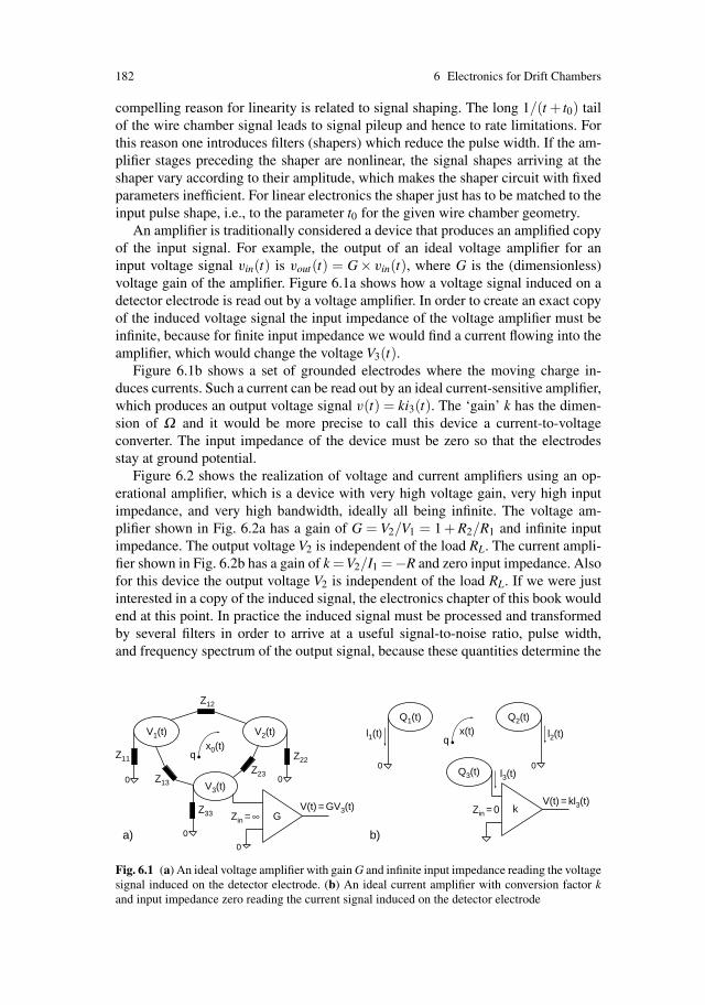
182 6 Electronics for Drift Chambers
compelling reason for linearity is related to signal shaping. The long 1/(t + t0) tailof the wire chamber signal leads to signal pileup and hence to rate limitations. Forthis reason one introduces filters (shapers) which reduce the pulse width. If the am-plifier stages preceding the shaper are nonlinear, the signal shapes arriving at theshaper vary according to their amplitude, which makes the shaper circuit with fixedparameters inefficient. For linear electronics the shaper just has to be matched to theinput pulse shape, i.e., to the parameter t0 for the given wire chamber geometry.
An amplifier is traditionally considered a device that produces an amplified copyof the input signal. For example, the output of an ideal voltage amplifier for aninput voltage signal vin(t) is vout(t) = G× vin(t), where G is the (dimensionless)voltage gain of the amplifier. Figure 6.1a shows how a voltage signal induced on adetector electrode is read out by a voltage amplifier. In order to create an exact copyof the induced voltage signal the input impedance of the voltage amplifier must beinfinite, because for finite input impedance we would find a current flowing into theamplifier, which would change the voltage V3(t).
Figure 6.1b shows a set of grounded electrodes where the moving charge in-duces currents. Such a current can be read out by an ideal current-sensitive amplifier,which produces an output voltage signal v(t) = ki3(t). The ‘gain’ k has the dimen-sion of Ω and it would be more precise to call this device a current-to-voltageconverter. The input impedance of the device must be zero so that the electrodesstay at ground potential.
Figure 6.2 shows the realization of voltage and current amplifiers using an op-erational amplifier, which is a device with very high voltage gain, very high inputimpedance, and very high bandwidth, ideally all being infinite. The voltage am-plifier shown in Fig. 6.2a has a gain of G = V2/V1 = 1 + R2/R1 and infinite inputimpedance. The output voltage V2 is independent of the load RL. The current ampli-fier shown in Fig. 6.2b has a gain of k =V2/I1 =−R and zero input impedance. Alsofor this device the output voltage V2 is independent of the load RL. If we were justinterested in a copy of the induced signal, the electronics chapter of this book wouldend at this point. In practice the induced signal must be processed and transformedby several filters in order to arrive at a useful signal-to-noise ratio, pulse width,and frequency spectrum of the output signal, because these quantities determine the
qx(t)
k
V1(t) V2(t)Q1(t)
l1(t) l2(t)
l3(t)
Q2(t)
Q3(t)
V(t) = GV3(t)V(t) = kl3(t)
V3(t)
qx0(t)
0
0
0
0
0 0
Z12
Z11
Z13
Z33 Zin = ∞Zin = 0
Z23
Z22
G
a) b)
Fig. 6.1 (a) An ideal voltage amplifier with gain G and infinite input impedance reading the voltagesignal induced on the detector electrode. (b) An ideal current amplifier with conversion factor kand input impedance zero reading the current signal induced on the detector electrode
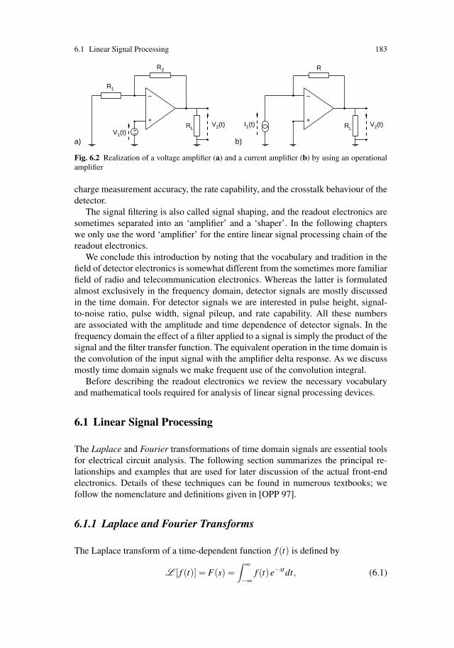
6.1 Linear Signal Processing 183
+
–
+–V1(t)
R1
R2
RL
+
–
I1(t)
R
RL
a) b)
V2(t) V2(t)
Fig. 6.2 Realization of a voltage amplifier (a) and a current amplifier (b) by using an operationalamplifier
charge measurement accuracy, the rate capability, and the crosstalk behaviour of thedetector.
The signal filtering is also called signal shaping, and the readout electronics aresometimes separated into an ‘amplifier’ and a ‘shaper’. In the following chapterswe only use the word ‘amplifier’ for the entire linear signal processing chain of thereadout electronics.
We conclude this introduction by noting that the vocabulary and tradition in thefield of detector electronics is somewhat different from the sometimes more familiarfield of radio and telecommunication electronics. Whereas the latter is formulatedalmost exclusively in the frequency domain, detector signals are mostly discussedin the time domain. For detector signals we are interested in pulse height, signal-to-noise ratio, pulse width, signal pileup, and rate capability. All these numbersare associated with the amplitude and time dependence of detector signals. In thefrequency domain the effect of a filter applied to a signal is simply the product of thesignal and the filter transfer function. The equivalent operation in the time domain isthe convolution of the input signal with the amplifier delta response. As we discussmostly time domain signals we make frequent use of the convolution integral.
Before describing the readout electronics we review the necessary vocabularyand mathematical tools required for analysis of linear signal processing devices.
6.1 Linear Signal Processing
The Laplace and Fourier transformations of time domain signals are essential toolsfor electrical circuit analysis. The following section summarizes the principal re-lationships and examples that are used for later discussion of the actual front-endelectronics. Details of these techniques can be found in numerous textbooks; wefollow the nomenclature and definitions given in [OPP 97].
6.1.1 Laplace and Fourier Transforms
The Laplace transform of a time-dependent function f (t) is defined by
L [ f (t)] = F(s) =∫ ∞
−∞f (t)e−stdt, (6.1)

184 6 Electronics for Drift Chambers
where s is a complex number with real part σ and an imaginary part ω: s = σ + iω .This definition is called the ‘bilateral’ Laplace transform because the integration ex-tends from −∞ to ∞. In the case where f (t) = 0 for t < 0 the transform is equal to theunilateral Laplace transform, which has a lower integration limit of 0. While F(s)has no direct physical interpretation, the Fourier transform of the signal, defined by
F [ f (t)] =∫ ∞
−∞f (t)e−iωtdt = F(iω) ω = 2π f , (6.2)
expresses the signal as a superposition of sinusoidal waves of frequency f with am-plitudes |F(iω)| and relative phases arg[F(iω)]. The Fourier transform is a specialcase of the bilateral Laplace transform with σ = 0. The inverse transforms are
f (t) =1
2πi
∫ σ+i∞
σ−i∞F(s)est ds f (t) =
12π
∫ ∞
−∞F(iω)eiωt dω. (6.3)
The transformations of the most common functions are tabulated in standard text-books. For the Laplace and Fourier transforms, the following relations hold (proofscan be found in [OPP 97]):
(a) Addition (b) ConvolutionL [a f (t)+bg(t)] = aF(s)+bG(s) L
[∫ ∞−∞ f (t − t ′)g(t ′)dt ′
]= F(s)G(s)
(c) Time differentiation (d) Time integration
L[
f (n)(t)]
= snF(s) L[∫ t
−∞ f (t ′)dt ′]= 1
s F(s)
(e) Time shift (f) Time scalingL [ f (t − t0)] = F(s)e−st0 L [ f (at)] = 1
a F( sa )
(g) Damping (h) MultiplicationL [e−s0t f (t)] = F(s+ s0) L [tn f (t)] = (−1)nF(n)(s)
(i) Initial value if f (t) = 0 for t < 0 (j) Final valuef (0+) = lim
s→∞sF(s) f (∞) = lim
s→0sF(s)
(k) Parseval’s theorem∫ ∞−∞ f (t)2dt =
∫ ∞−∞ |F(i2π f )|2d f = 2
∫ ∞0 |F(i2π f )|2d f
(6.4)The usefulness of these transformations for electrical circuit analysis is illustrated
by the following example. The voltage vR(t) across a resistor R for an impressed cur-rent i(t) is given by Ohm’s law as vR(t) = Ri(t). The voltage across a capacitor C foran impressed current i(t) is vC(t) = 1/C
∫i(t)dt. The voltage across an inductance
L for an impressed current i(t) is given by vL(t) = Ldi(t)/dt. Voltages and currentsin a circuit containing R,L, and C elements are determined by applying Kirchhoff’slaws, which state that the sum of voltages in every loop must be zero and the sumof the currents on every node must be zero. This analysis therefore leads to a set oflinear differential equations for the currents and voltages in the circuit.

6.1 Linear Signal Processing 185
Writing the above relations in the Laplace domain, we find VR(s) = RI(s),VC(s) = I(s)/sC, and VL(s) = sLI(s), and the circuit relations become algebraicequations. Instead of having to solve a set of coupled differential equations in thetime domain we just have to solve a set of linear algebraic equations in the Laplacedomain! In addition, owing to the theorems stated above, many signal manipulationsare strongly simplified when working in the Laplace domain.
Finally we define the impedance Z(s) of a circuit element as Z(s) = V (s)/I(s).We find the impedance of ZC(s) = 1/sC for a capacitor and ZL(s) = sL for an in-ductor. In analogy to the resistance R1 + R2 of two resistors switched in series, thetotal impedance of two impedances Z1 and Z2 switched in series is Z1 + Z2. Like-wise, the parallel application of the impedances gives a total impedance of Z1Z2/(Z1 +Z2).
6.1.2 Transfer Functions, Poles and Zeros, Delta Response
We now want to read out the chamber output signal i(t) with a general linear signalprocessing device. Such a signal is, e.g., the current signal i(t) of the drift tubeindicated in Fig. 5.10. A linear device is defined by the following property: if theinput signals i1(t) and i2(t) result in output signals v1(t) and v2(t), the input signali(t) = c1i1(t)+ c2i2(t) will result in the output signal v(t) = c1v1(t)+ c2v2(t).
The input and output signals of a linear, time-invariant, and causal device arerelated by a differential equation of the following form:
a0 v(t)+a1dv(t)
dt+ . . .+am
dmv(t)dtm = b0 i(t)+b1
di(t)dt
+ . . .+bndni(t)
dtn , (6.5)
where the coefficients a and b are independent of time. The term ‘time-invariant’describes the fact that the relation between input and output signals is independentof time. For a ‘causal’ system the output signal v(t) is zero as long as the inputsignal i(t) is zero.
Performing the Laplace transform and using Eq. (6.4c) transforms this equationinto an algebraic equation with the solution
V (s) =b0 +b1s+ . . .+bnsn
a0 +a1s+ . . .+amsm I(s) = W (s)I(s), (6.6)
where we have defined L [i(t)] = I(s) and L [v(t)] = V (s). The function W (s) iscalled the transfer function of the system and we see that the transfer function of alinear time-invariant system can be expressed by the ratio of two polynomials in theLaplace domain.
Setting s = iω yields the transfer function in the Fourier domain and the relation-ship between input and output signals is
V (iω) = W (iω) I(iω). (6.7)
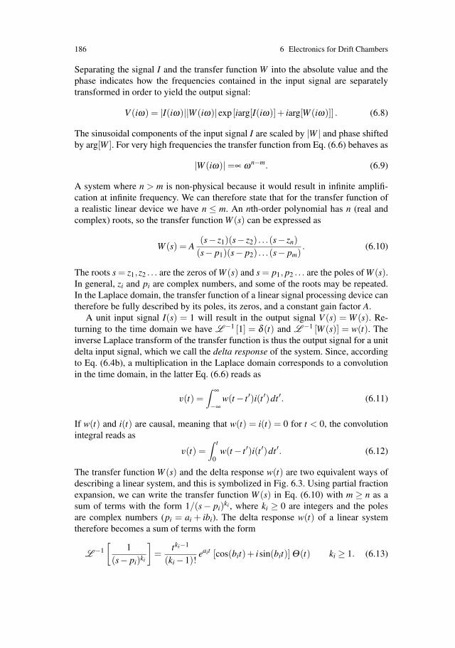
186 6 Electronics for Drift Chambers
Separating the signal I and the transfer function W into the absolute value and thephase indicates how the frequencies contained in the input signal are separatelytransformed in order to yield the output signal:
V (iω) = |I(iω)||W (iω)|exp [iarg[I(iω)]+ iarg[W (iω)]] . (6.8)
The sinusoidal components of the input signal I are scaled by |W | and phase shiftedby arg[W ]. For very high frequencies the transfer function from Eq. (6.6) behaves as
|W (iω)| =∝ ωn−m. (6.9)
A system where n > m is non-physical because it would result in infinite amplifi-cation at infinite frequency. We can therefore state that for the transfer function ofa realistic linear device we have n ≤ m. An nth-order polynomial has n (real andcomplex) roots, so the transfer function W (s) can be expressed as
W (s) = A(s− z1)(s− z2) . . .(s− zn)
(s− p1)(s− p2) . . .(s− pm). (6.10)
The roots s = z1,z2 . . . are the zeros of W (s) and s = p1, p2 . . . are the poles of W (s).In general, zi and pi are complex numbers, and some of the roots may be repeated.In the Laplace domain, the transfer function of a linear signal processing device cantherefore be fully described by its poles, its zeros, and a constant gain factor A.
A unit input signal I(s) = 1 will result in the output signal V (s) = W (s). Re-turning to the time domain we have L −1 [1] = δ (t) and L −1 [W (s)] = w(t). Theinverse Laplace transform of the transfer function is thus the output signal for a unitdelta input signal, which we call the delta response of the system. Since, accordingto Eq. (6.4b), a multiplication in the Laplace domain corresponds to a convolutionin the time domain, in the latter Eq. (6.6) reads as
v(t) =∫ ∞
−∞w(t − t ′)i(t ′)dt ′. (6.11)
If w(t) and i(t) are causal, meaning that w(t) = i(t) = 0 for t < 0, the convolutionintegral reads as
v(t) =∫ t
0w(t − t ′)i(t ′)dt ′. (6.12)
The transfer function W (s) and the delta response w(t) are two equivalent ways ofdescribing a linear system, and this is symbolized in Fig. 6.3. Using partial fractionexpansion, we can write the transfer function W (s) in Eq. (6.10) with m ≥ n as asum of terms with the form 1/(s− pi)ki , where ki ≥ 0 are integers and the polesare complex numbers (pi = ai + ibi). The delta response w(t) of a linear systemtherefore becomes a sum of terms with the form
L −1[
1(s− pi)ki
]=
tki−1
(ki −1)!eait [cos(bit)+ isin(bit)] Θ(t) ki ≥ 1. (6.13)

6.1 Linear Signal Processing 187
i(t)
I(s)
w(t)
W(s)
o(t) = ∫w(t-t')i(t')dt'
O(s) = W(s) I(s)
Fig. 6.3 A linear device is characterized by the transfer function W (s) in the Laplace domain orthe delta response w(t) = L −1 [W (s)] in the time domain
The step function Θ(t) is defined in Eq. (6.16). For k = 0 we have L −1 [1] = δ (t).If ai > 0, the delta response tends to infinity for t → ∞, so the criterion for stabilityof a linear system is given by the requirement that the real parts of all poles of W (s)must be negative. In the case where ai + ibi is a root of a polynomial, the complexconjugate ai − ibi is also a root of the polynomial. Thus the terms in Eq. (6.13)always appear in complex conjugate pairs, the imaginary part is cancelled, and thedelta response is always real.
Figure 6.4 shows an example of the terms from Eq. (6.13) for k = 2,4,6 and bi =0. In this book we mainly discuss transfer functions with real poles. The imaginaryparts of poles arise from inductances. (As these cannot be implemented physically ascoils in integrated devices, one would make them feedback loops using operationalamplifiers).
6.1.3 CR, RC, Pole-zero and Zero-pole Filters
In this section we discuss four elementary filters that illustrate the formalism out-lined in the previous section. They are also elementary in the sense that by cascadingthese four filter types we can construct any desired transfer function W (s) with realpoles. If we wanted to construct the most general transfer function W (s) also in-cluding complex poles we would have to add a few elementary circuits containingan inductance L. The CR and RC filters are shown in Fig. 6.5. The output voltagesof the two filters for an input voltage signal V (s) = L [v(t)] are
Fig. 6.4 The delta responsew(t) of a linear network withreal poles consists of the sumof shapes indicated in thisfigure. In the case whereW (s) has complex poles wefind terms with an oscillatorybehaviour of frequency bi/2πand a damping factor ofexp(−ait) 1 2 3 4 5
0.2
0.4
0.6
0.8
1
k = 6
t/tp
k = 4k = 2
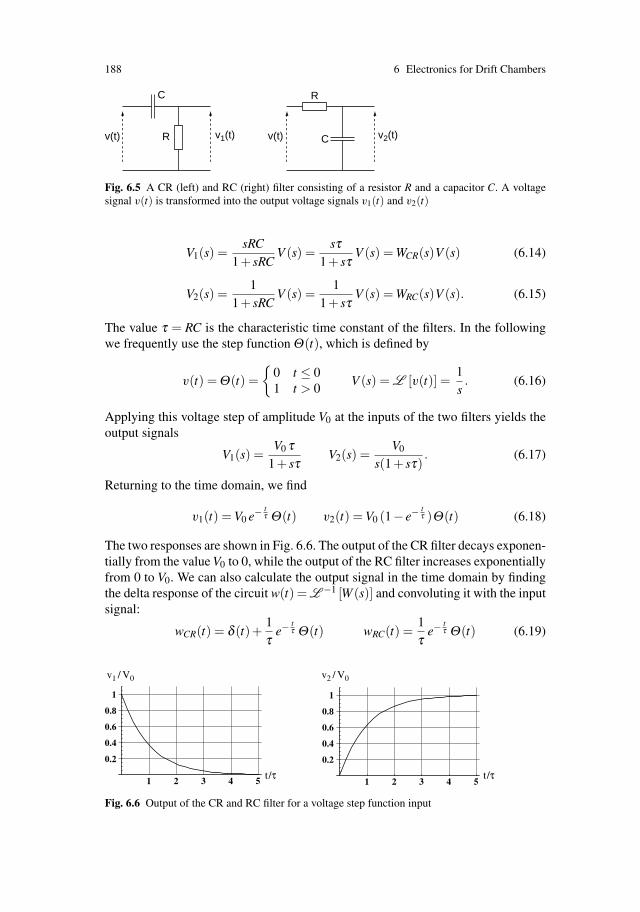
188 6 Electronics for Drift Chambers
R
R C
C
v(t)v(t) v1(t) v2(t)
Fig. 6.5 A CR (left) and RC (right) filter consisting of a resistor R and a capacitor C. A voltagesignal v(t) is transformed into the output voltage signals v1(t) and v2(t)
V1(s) =sRC
1+ sRCV (s) =
sτ1+ sτ
V (s) = WCR(s)V (s) (6.14)
V2(s) =1
1+ sRCV (s) =
11+ sτ
V (s) = WRC(s)V (s). (6.15)
The value τ = RC is the characteristic time constant of the filters. In the followingwe frequently use the step function Θ(t), which is defined by
v(t) = Θ(t) ={
0 t ≤ 01 t > 0
V (s) = L [v(t)] =1s. (6.16)
Applying this voltage step of amplitude V0 at the inputs of the two filters yields theoutput signals
V1(s) =V0 τ
1+ sτV2(s) =
V0
s(1+ sτ). (6.17)
Returning to the time domain, we find
v1(t) = V0 e−tτ Θ(t) v2(t) = V0 (1− e−
tτ )Θ(t) (6.18)
The two responses are shown in Fig. 6.6. The output of the CR filter decays exponen-tially from the value V0 to 0, while the output of the RC filter increases exponentiallyfrom 0 to V0. We can also calculate the output signal in the time domain by findingthe delta response of the circuit w(t) = L −1 [W (s)] and convoluting it with the inputsignal:
wCR(t) = δ (t)+1τ
e−tτ Θ(t) wRC(t) =
1τ
e−tτ Θ(t) (6.19)
1 2 3 4 5
0.2
0.4
0.6
0.8
1
1 2 3 4 5
0.2
0.4
0.6
0.8
1
v1 / V0 v2 / V0
t /τ t /τ
Fig. 6.6 Output of the CR and RC filter for a voltage step function input

6.1 Linear Signal Processing 189
v1(t) =∫ t
0
(δ (t − t ′)− 1
τe−
t−t′τ Θ(t − t ′)
)V0 Θ(t ′)dt ′= V0 e−
tτ Θ(t)
v2(t) =∫ t
0
(1τ
e−t−t′
τ Θ(t − t ′))
V0 Θ(t ′)dt ′ = V0 (1− e−tτ )Θ(t) . (6.20)
We find the same result as before. If we replace s by iω we have the transfer functionin the Fourier (frequency) domain:
WCR(iω) =iω τ
1+ iωτ=
ωτ√1+ω2τ2
exp [i arctan1/ωτ],
WRC(iω) =1
1+ iωτ=
1√1+ω2τ2
exp [i arctanωτ].(6.21)
The absolute values and the phases of the transfer functions are shown in Fig. 6.7.At the frequency ω0 = 1/τ , the input voltage is attenuated by 1/
√2 ≈ 0.707 by
both filters. The CR filter attenuates frequencies ω < ω0 while high frequenciesare passing the circuit, so the CR circuit is called a high-pass filter. The RC circuitpasses low frequencies and attenuates high frequencies and is called a low-passfilter. At the frequency ω0, the phase shift between the input and the output voltageis arctan(1) = π/4 = 45o.
From Eq. (6.4c,d) we know that the differentiation in the time domain corre-sponds to a multiplication with s in the Laplace domain and that the integration inthe time domain corresponds to division by s in the Laplace domain. The transferfunction of a ‘differentiator’ or ‘integrator’ is therefore s or 1/s. The RC filter there-fore becomes an integrator for large values of τ , or more precisely if the frequency1/τ is much lower than all the frequencies contained in the signal. The CR circuitapproaches a differentiator if τ is small, i.e., if the frequency 1/τ is much higherthan the frequencies contained in the input signal.
To conclude this section we investigate the pole-zero and zero-pole filters shownin Fig. 6.8, which are used extensively for signal shaping. The transfer functions ofthe two filters are given by
0.01 0.1 1 10 1000
20
40
60
80
Phase deg
CR RC
0.01 0.1 1 10 1000
0.2
0.4
0.6
0.8
1
W
CR RC
ωτ ωτ
Fig. 6.7 Absolute value and phase of the transfer function for an RC (low-pass) and a CR (high-pass) filter. At the frequency ω0 = 1/τ the input voltage is attenuated by 1/
√2 ≈ 0.707 and the
phase shift between the input and the output signal is π/4 = 45o
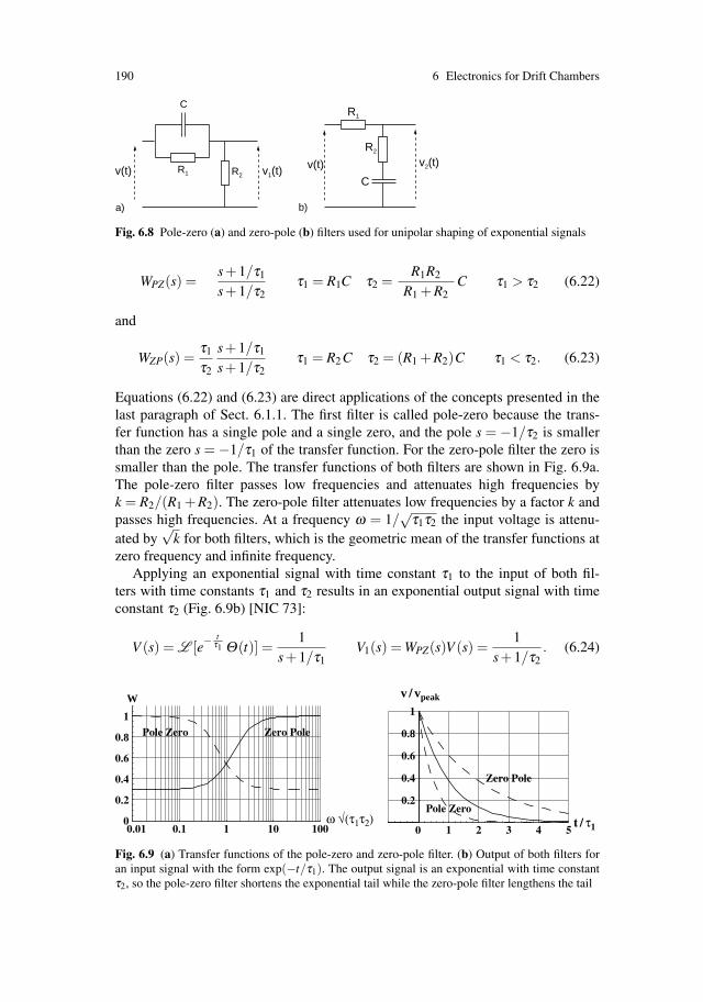
190 6 Electronics for Drift Chambers
R1
R1
C
C
v(t)v(t) v1(t)v2(t)R2
R2
a) b)
Fig. 6.8 Pole-zero (a) and zero-pole (b) filters used for unipolar shaping of exponential signals
WPZ(s) =s+1/τ1
s+1/τ2τ1 = R1C τ2 =
R1R2
R1 +R2C τ1 > τ2 (6.22)
and
WZP(s) =τ1
τ2
s+1/τ1
s+1/τ2τ1 = R2 C τ2 = (R1 +R2)C τ1 < τ2. (6.23)
Equations (6.22) and (6.23) are direct applications of the concepts presented in thelast paragraph of Sect. 6.1.1. The first filter is called pole-zero because the trans-fer function has a single pole and a single zero, and the pole s = −1/τ2 is smallerthan the zero s = −1/τ1 of the transfer function. For the zero-pole filter the zero issmaller than the pole. The transfer functions of both filters are shown in Fig. 6.9a.The pole-zero filter passes low frequencies and attenuates high frequencies byk = R2/(R1 +R2). The zero-pole filter attenuates low frequencies by a factor k andpasses high frequencies. At a frequency ω = 1/
√τ1τ2 the input voltage is attenu-
ated by√
k for both filters, which is the geometric mean of the transfer functions atzero frequency and infinite frequency.
Applying an exponential signal with time constant τ1 to the input of both fil-ters with time constants τ1 and τ2 results in an exponential output signal with timeconstant τ2 (Fig. 6.9b) [NIC 73]:
V (s) = L [e−t
τ1 Θ(t)] =1
s+1/τ1V1(s) = WPZ(s)V (s) =
1s+1/τ2
. (6.24)
0.01 0.1 1 10 1000
0.2
0.4
0.6
0.8
1
W
Pole Zero Zero Pole
1 2 3 4 5
0.2
0.4
0.6
0.8
1
Zero Pole
Pole Zerot / τ1
ω √(τ1τ2)
v / vpeak
0
Fig. 6.9 (a) Transfer functions of the pole-zero and zero-pole filter. (b) Output of both filters foran input signal with the form exp(−t/τ1). The output signal is an exponential with time constantτ2, so the pole-zero filter shortens the exponential tail while the zero-pole filter lengthens the tail
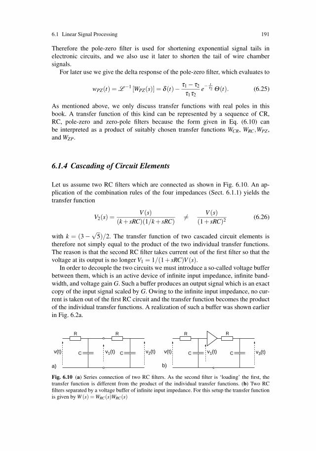
6.1 Linear Signal Processing 191
Therefore the pole-zero filter is used for shortening exponential signal tails inelectronic circuits, and we also use it later to shorten the tail of wire chambersignals.
For later use we give the delta response of the pole-zero filter, which evaluates to
wPZ(t) = L −1 [WPZ(s)] = δ (t)− τ1 − τ2
τ1τ2e− t
τ2 Θ(t). (6.25)
As mentioned above, we only discuss transfer functions with real poles in thisbook. A transfer function of this kind can be represented by a sequence of CR,RC, pole-zero and zero-pole filters because the form given in Eq. (6.10) canbe interpreted as a product of suitably chosen transfer functions WCR, WRC,WPZ ,and WZP.
6.1.4 Cascading of Circuit Elements
Let us assume two RC filters which are connected as shown in Fig. 6.10. An ap-plication of the combination rules of the four impedances (Sect. 6.1.1) yields thetransfer function
V2(s) =V (s)
(k + sRC)(1/k + sRC)�= V (s)
(1+ sRC)2 (6.26)
with k = (3 −√
5)/2. The transfer function of two cascaded circuit elements istherefore not simply equal to the product of the two individual transfer functions.The reason is that the second RC filter takes current out of the first filter so that thevoltage at its output is no longer V1 = 1/(1+ sRC)V (s).
In order to decouple the two circuits we must introduce a so-called voltage bufferbetween them, which is an active device of infinite input impedance, infinite band-width, and voltage gain G. Such a buffer produces an output signal which is an exactcopy of the input signal scaled by G. Owing to the infinite input impedance, no cur-rent is taken out of the first RC circuit and the transfer function becomes the productof the individual transfer functions. A realization of such a buffer was shown earlierin Fig. 6.2a.
R
Cv(t) v2(t) v1(t) v3(t)v1(t)
R
C
R
Cv(t)
R
C
a) b)
Fig. 6.10 (a) Series connection of two RC filters. As the second filter is ‘loading’ the first, thetransfer function is different from the product of the individual transfer functions. (b) Two RCfilters separated by a voltage buffer of infinite input impedance. For this setup the transfer functionis given by W (s) = WRC(s)WRC(s)

192 6 Electronics for Drift Chambers
We conclude that a cascade of circuit elements with individual transfer functionsW1(s),W2(s) . . .Wn(s), which are decoupled by ideal voltage buffers, has a transferfunction equal to the product
W (s) = W1(s)×W2(s)× . . .×Wn(s) . (6.27)
6.1.5 Amplifier Types, Bandwidth, Sensitivity, and Ballistic Deficit
The practical realizations of linear signal processing systems discussed above areamplifiers and filter circuits connected to the detector electrodes. Parameters thatcharacterize these devices, such as gain and bandwidth, have a range of differingdefinitions in the literature on microelectronics. We therefore review and define thevocabulary for the discussion of detector electronics.
Bandwidth Limit: In the frequency domain, an amplifier is characterized by thegain |W (iω)| and the phase shift arg[W (iω)] for each frequency. The bandwidthlimit of an amplifier is defined as the frequency at which the signal transmission hasbeen reduced by 3 dB from the central or midrange reference value. Since the powerlevel is defined as 10log(P/Pre f ) dB and the voltage level as 20log(V/Vre f )dB,a 3dB reduction corresponds to a power level of ≈ 0.5 and a voltage level equalto ≈ 0.708 ≈ 1/
√2 of the value at the centre frequency reference [MOT 93]. The
bandwidth limit of the RC low-pass filter is thus given by fbw = 1/2πτ = 1/2πRC.Rise Time, Peaking Time: The rise time tr of a pulse is defined as the time taken
for its leading edge to rise from 10 to 90% of the peak height. The peaking time tp
of a pulse is defined as the time taken for its leading edge to rise from zero to peakheight. When we talk about the peaking time of an amplifier we mean the peakingtime of its delta response.
Voltage, Current, and Charge Amplifiers: A voltage amplifier processes avoltage signal presented at its input and is characterized by high input impedance.A current amplifier processes the current signal flowing into the amplifier and ischaracterized by low input impedance. The signals in wire chambers are inducedcurrent signals, as discussed in the previous chapter. The example of the drift tube inSect. 5.6.1 shows that the detector capacitance Cdet together with the input resistanceRin forms an integration stage with bandwidth limit of fbw = 1/2πRinCdet , which isundesirable if one wants to preserve the fast signal. In order to preserve the chambersignal shape, the input impedance of the amplifier must be small compared to allother impedances in the detector or in the ideal case, equal to zero, which meansthat we use current amplifiers for readout of wire chambers. If the bandwidth ofthe current amplifier is such that it integrates a significant fraction of the chambersignal, or the entire chamber signal, it is usually called a charge amplifier.
Sensitivity of Current and Charge Amplifiers: The filters discussed in theprevious sections transform an input voltage signal to an output voltage signal, andtherefore the dimension of the transfer function is [W (s)] = 1. The transfer functionof a current amplifier that transforms a current input signal into a voltage outputsignal can be written as V (s) = kW (s)I(s), where k has dimensions of V/A=Ω and

6.1 Linear Signal Processing 193
W (s) keeps the dimension 1. In the time domain the relationship between the inputand output signals is
v(t) = k∫
w(t − t ′)i(t ′)dt ′ = kw(tp)∫
w(t − t ′)w(tp)
i(t ′)dt ′ = g∫
h(t − t ′)i(t ′)dt ′.
(6.28)
The value w(tp) is the peak of the delta response w(t), and the dimensionless func-tion h(t) is the normalized delta response. An input current pulse of i(t) = Qδ (t)results in an amplifier output peak voltage of v(tp) = gQ. We call g which has thedimension V/C, the sensitivity of the amplifier, Typical wire chamber amplifiershave sensitivities in the range of 1–50 mV/fC.
Ballistic Deficit: If a current amplifier has a peaking time tp which is muchlonger than the duration of the input current signal i(t), the convolution integral canbe approximated and the output pulse is given by
v(t) = g∫
h(t − t ′)i(t ′)dt ′ ≈ gh(t)∫
i(t ′)dt ′ = gh(t)Qtot . (6.29)
The peak of the output signal is gQtot . The output pulse height is therefore propor-tional to the total signal charge and such an amplifier is called a charge amplifier.For timing purposes or due to high signal rates, one typically wants to preserve thesignal speed and keep the pulse width to a minimum. Although the amplifiers usedfor wire chambers will always have peaking times shorter than the maximum drifttime of the ions, an amplifier that integrates a significant fraction of the inducedcharge is traditionally still called a charge amplifier.
As long peaking times limit the rate capability of a detector one usually has tolive with a compromise between pulse-width and charge measurement accuracy.The incomplete measurement of the signal charge is characterized by the so-calledballistic deficit, which is defined as the difference between the amplifier output pulseheight for the input signal i(t) and the output pulse height if the entire input signalcharge Qtot =
∫i(t)dt is contained in a delta current pulse Qtotδ (t).
Equivalent Block Diagram: In Sect. 6.1.1 we saw that the transfer functionW (s) of a linear electronic circuit is specified by an expression of the form
W (s) = A(s− z1)(s− z2) . . .(s− zn)
(s− p1)(s− p2) . . .(s− pm). (6.30)
Let us now assume that we have defined such a transfer function and we want tofind an electronic circuit realization of it. As an example we assume that we want totransform a voltage signal V1(s) by the transfer function
V2(s) = W (s)V1(s) = Gs+α
(s+β )(s+ γ)V1(s), (6.31)
where α,β , and γ are positive and real. We can interpret W (s) as the product of apole-zero filter and an RC filter, so a possible realization of this transfer functioncan be seen in Fig. 6.11, where a pole-zero and an RC filter are coupled by an

194 6 Electronics for Drift Chambers
Fig. 6.11 Cascade of an RCfilter and a pole-zero filter
C
v(t) v1(t)R2R1
R
C
G
ideal voltage buffer of gain G. Such a representation is of course not unique andthere are several ways to realize a transfer function. The important point is that anytransfer function can be represented by a cascade of simple, elementary circuits,which facilitates the circuit analysis and serves as a basis for the actual design.
Up to now we have investigated filters that convert voltage input signals into volt-age output signals. However, the signals induced on chamber electrodes are currentsignals, so for our block diagram representation we need an idealized device whichconverts a current input signal into a voltage signal. We assume an idealized devicewith infinite bandwidth such that for a current input signal i(t) we get a voltageoutput signal v(t) = ki(t). With this device we can complete our block diagram rep-resentation of the detector readout electronics (Fig. 6.12). In principle this kind ofblock diagram can also be used for a practical realization, where the voltage bufferand current to voltage converter are devices with a bandwidth that must be broaderthan the bandwidth of the other circuit elements. Although most designs of chamberelectronics consist of cascaded blocks with intermediate buffers, there are numerousdifferent ways of realizing the individual transfer functions. As outlined earlier, thegoal of this chapter is not the design a practical realization of the readout electronicsbut its precise specification. The block diagram defined above serves as a basis forthe circuit realization.
6.2 Signal Shaping
The transfer function W (s) of the readout electronics must be chosen in order tooptimize the measurement of the quantity of interest, such as signal charge or signaltime. For this discussion the electronics noise plays a key role, and we have tocharacterize noise sources and apply the theory of optimum filtering. Parameters
R1 R2
C
R
C v1(t)
Gk
i(t)
v(t) = k i(t)
Fig. 6.12 An ideal current to voltage converter followed by a CR and pole-zero filter
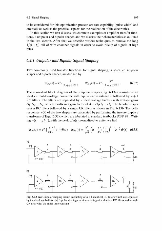
6.2 Signal Shaping 195
to be considered for this optimization process are rate capability (pulse width) andcrosstalk as well as the practical aspects for the realization of the electronics.
In this section we first discuss two common examples of amplifier transfer func-tions, a unipolar and bipolar shaper, and we discuss their characteristics as outlinedin the last section. After that we describe various techniques to remove the long1/(t + t0) tail of wire chamber signals in order to avoid pileup of signals at highrates.
6.2.1 Unipolar and Bipolar Signal Shaping
Two commonly used transfer functions for signal shaping, a so-called unipolarshaper and bipolar shaper, are defined by
Wuni(s) = kA1
(1+ sτ)n+1 Wbip(s) = kAsτ
(1+ sτ)n+1 . (6.32)
The equivalent block diagram of the unipolar shaper (Fig. 6.13a) consists of anideal current-to-voltage converter with equivalent resistance k followed by n + 1RC filters. The filters are separated by n ideal voltage buffers with voltage gainsG1,G2 . . .Gn, which results in a gain factor of A = G1G2 . . .Gn. The bipolar shaperuses n RC filters followed by a single CR filter, as shown in Fig. 6.13b. The deltaresponses w(t) of the two shapers are calculated by performing the inverse Laplacetransforms of Eqs. (6.32), which are tabulated in standard textbooks [OPP 97]. Writ-ing w(t) = gh(t), with the peak of h(t) normalized to unity, we find
huni(t) = en( t
nτ
)ne−
tτ Θ(t) hbip(t) =
er√
n
(n− t
τ
)( trτ
)n−1e−
tτ Θ(t) (6.33)
k
1
R
C
i(t)
i(t)
v = k i(t)
R
C
R
C
....
v(t)
v(t)
2 n n+1
R
C
a)
1
R
C
R
C R
C....
2 n
R
C
k
v = k i(t)
b)
G1
G1
G2
G2
Gn
Gn
Fig. 6.13 (a) Unipolar shaping circuit consisting of n+1 identical RC filters which are separatedby ideal voltage buffers. (b) Bipolar shaping circuit consisting of n identical RC filters and a singleCR filter with the same time constant
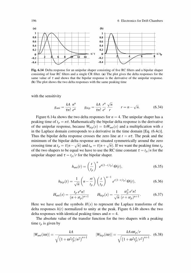
196 6 Electronics for Drift Chambers
2 4 6 8 10 12 14
0.2
0.4
0.6
0.8
1
(a) (b)
2 4 6 8
–0.4
–0.2
–0.4
–0.2
0.2
0.4
0.6
0.8
1
t / tpt / τ 00
Fig. 6.14 Delta response for an unipolar shaper consisting of five RC filters and a bipolar shaperconsisting of four RC filters and a single CR filter. (a) The plot gives the delta responses for thesame value of τ and shows that the bipolar response is the derivative of the unipolar response.(b) The plot shows the two delta responses with the same peaking time
with the sensitivity
guni =kAτn!
nn
en gbip =kAτn!
rn
er
√n
rr = n−
√n. (6.34)
Figure 6.14a shows the two delta responses for n = 4. The unipolar shaper has apeaking time of tp = nτ . Mathematically the bipolar delta response is the derivativeof the unipolar response, because Wbip(s) = τsWuni(s) and a multiplication with sin the Laplace domain corresponds to a derivative in the time domain [Eq. (6.4c)].Thus the bipolar delta response crosses the zero line at t = nτ . The peak and theminimum of the bipolar delta response are situated symmetrically around the zerocrossing time at tp = τ(n−√
n) and tm = τ(n+√
n). If we want the peaking time tp
of the two shapers to be equal we have to use the RC time constant τ = tp/n for theunipolar shaper and τ = tp/r for the bipolar shaper.
huni(t) =(
ttp
)n
en(1−t/tp)Θ(t), (6.35)
hbip(t) =1√n
(n− rt
tp
)(ttp
)n−1
er(1−t/tp)Θ(t), (6.36)
Huni(s) =tp enn!
(n+ stp)n+1 Hbip(s) =1√n
st2p ern!
(r + stp)n+1 . (6.37)
Here we have used the symbols H(s) to represent the Laplace transforms of thedelta responses h(t) normalized to unity at the peak. Figure 6.14b shows the twodelta responses with identical peaking times and n = 4.
The absolute value of the transfer function for the two shapers with a peakingtime tp is given by
|Wuni(iω)| = kA√(1+ω2t2
p/n2)n+1
|Wbip(iω)| = kAωtp/r√(1+ω2t2
p/r2)n+1
. (6.38)
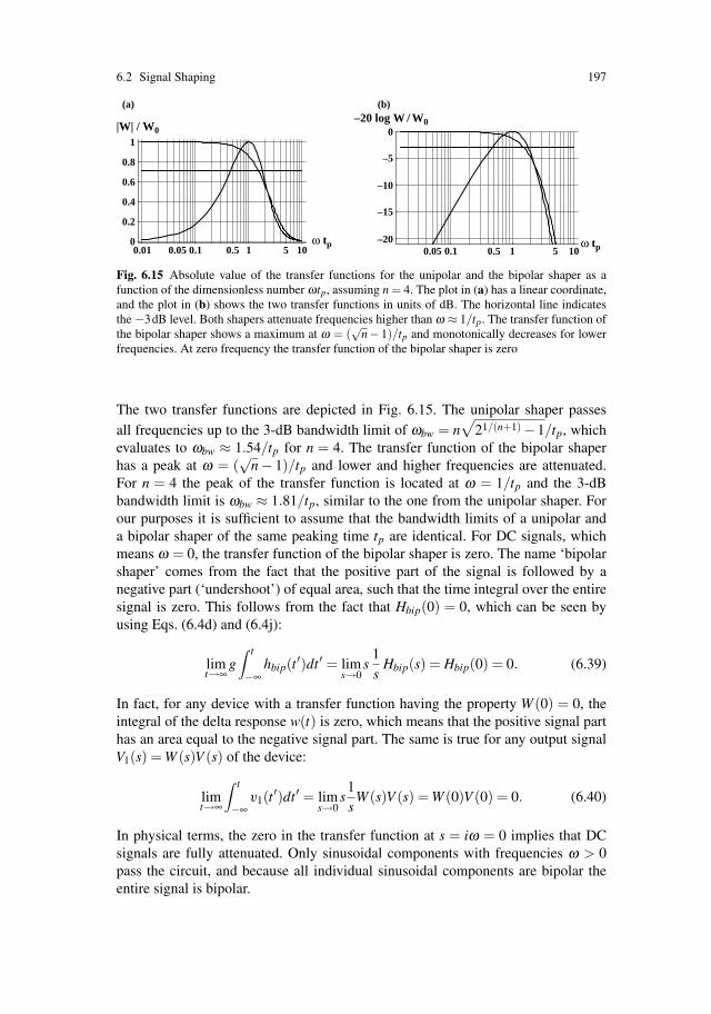
6.2 Signal Shaping 197
0.01 0.05 0.1 0.5 1 5 100
0.2
0.4
0.6
0.8
1
0.05 0.1 0.5 1 5 10
–10
0|W| / W0–20 log W / W0
ω tpω tp
–5
–15
–20
(a) (b)
Fig. 6.15 Absolute value of the transfer functions for the unipolar and the bipolar shaper as afunction of the dimensionless number ωtp, assuming n = 4. The plot in (a) has a linear coordinate,and the plot in (b) shows the two transfer functions in units of dB. The horizontal line indicatesthe −3dB level. Both shapers attenuate frequencies higher than ω ≈ 1/tp. The transfer function ofthe bipolar shaper shows a maximum at ω = (
√n− 1)/tp and monotonically decreases for lower
frequencies. At zero frequency the transfer function of the bipolar shaper is zero
The two transfer functions are depicted in Fig. 6.15. The unipolar shaper passesall frequencies up to the 3-dB bandwidth limit of ωbw = n
√21/(n+1)−1/tp, which
evaluates to ωbw ≈ 1.54/tp for n = 4. The transfer function of the bipolar shaperhas a peak at ω = (
√n− 1)/tp and lower and higher frequencies are attenuated.
For n = 4 the peak of the transfer function is located at ω = 1/tp and the 3-dBbandwidth limit is ωbw ≈ 1.81/tp, similar to the one from the unipolar shaper. Forour purposes it is sufficient to assume that the bandwidth limits of a unipolar anda bipolar shaper of the same peaking time tp are identical. For DC signals, whichmeans ω = 0, the transfer function of the bipolar shaper is zero. The name ‘bipolarshaper’ comes from the fact that the positive part of the signal is followed by anegative part (‘undershoot’) of equal area, such that the time integral over the entiresignal is zero. This follows from the fact that Hbip(0) = 0, which can be seen byusing Eqs. (6.4d) and (6.4j):
limt→∞
g∫ t
−∞hbip(t ′)dt ′ = lim
s→0s
1s
Hbip(s) = Hbip(0) = 0. (6.39)
In fact, for any device with a transfer function having the property W (0) = 0, theintegral of the delta response w(t) is zero, which means that the positive signal parthas an area equal to the negative signal part. The same is true for any output signalV1(s) = W (s)V (s) of the device:
limt→∞
∫ t
−∞v1(t ′)dt ′ = lim
s→0s
1s
W (s)V (s) = W (0)V (0) = 0. (6.40)
In physical terms, the zero in the transfer function at s = iω = 0 implies that DCsignals are fully attenuated. Only sinusoidal components with frequencies ω > 0pass the circuit, and because all individual sinusoidal components are bipolar theentire signal is bipolar.

198 6 Electronics for Drift Chambers
A device with a transfer function W (s) having the property W (0) = 0 is called anAC coupled device. If W (0) is non-zero it is called DC coupled. The drift tube circuitdiscussed in Sect. 5.6.1 is an AC coupled system because the capacitor blocking thehigh voltage U from the amplifier also blocks the low-frequency components of thesignal.
In the following we discuss the processing of a wire chamber signal by the twoshapers discussed above. The currents flowing into the input of the readout electron-ics are typically not exactly equal to the current signals induced on the electrodes,but they are already ‘shaped’ by the effects of the passive detector elements pre-ceding the amplifier together with the input impedance of the amplifier. In order toavoid the complications of this input circuit, which we discuss later, we consider forthe moment only the drift tube from Sect. 5.5, where the tube wall is set to potential−U and the wire is grounded. We assume that the connection of the wire to groundis performed through a current amplifier of zero input impedance with transfer func-tion Wuni or Wbip. The induced current signal is therefore equal to the current flowinginto the amplifier and is given by the form
i(t) =q
2t0 ln(b/a)1
1+ t/t00 < t/t0 < tmax =
b2
a2 −1. (6.41)
As the Laplace transform of this signal cannot be written in closed form wecalculate the output signal by numerical evaluation of the convolution of i(t) withthe amplifier delta response. We assume the same sensitivity g and peaking timetp for the unipolar and bipolar shaper. We must therefore perform the convolutionof i(t) with ghuni(t) or ghbip(t), where we insert τ = tp/n for the unipolar andτ = tp/(n−√
n) for the bipolar shaper. We just present the integral for the unipolarshaper, which reads as
v(t) = g∫ t
0huni(t − t ′)i(t ′)dt ′ → (6.42)
v(t)gq
=1
2ln(b/a)
∫ t
0
[e
t0tp
(tt0− t ′
t0
)e− t0
tp
(t
t0− t′
t0
)]n 11+(t ′/t0)
dt ′
t0.
As an example we use a drift tube with a parameter b/a = 100, giving a valueof tmax = 104t0 for the signal duration. For a t0 value of 1 ns this evaluates to tmax =10 μs. Figure 6.16a shows the amplifier output signals for n = 4 and a value fortp/t0 = 10. For a t0 value of 1 ns this corresponds to an amplifier peaking time of10 ns. The bipolar signal returns to zero after a time of t/t0 ≈ 100, while the outputsignal of the unipolar shaper shows a very long tail that will lead to signal pileup athigh counting rates.
For our assumed parameters the signal has a peak of vp/gq = 0.22, which meansthat the ballistic deficit is 78%. Figure 6.16b shows the amplifier output signal forincreasing values of tp/t0. The longer the peaking time the larger the signal and thesmaller the ballistic deficit. For tp > tmax the signal peak approaches v = gq andthe ballistic deficit approaches zero. The pulse height is related to the signal charge
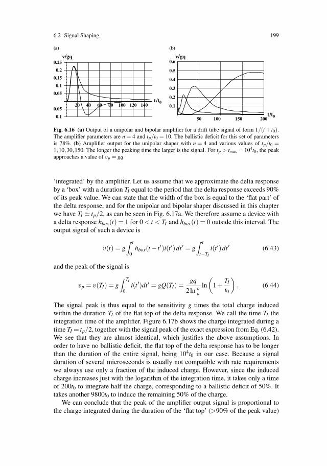
6.2 Signal Shaping 199
20 40 60 80 100 120 140
0.1
0.05
0.05
0.1
0.15
0.2
0.25
(a) (b)
50 100 150 200
0.1
0.2
0.3
0.4
0.5
0.6v/gq v/gq
t /t0
t /t0
Fig. 6.16 (a) Output of a unipolar and bipolar amplifier for a drift tube signal of form 1/(t + t0).The amplifier parameters are n = 4 and tp/t0 = 10. The ballistic deficit for this set of parametersis 78%. (b) Amplifier output for the unipolar shaper with n = 4 and various values of tp/t0 =1,10,30,150. The longer the peaking time the larger is the signal. For tp > tmax = 104t0, the peakapproaches a value of vp = gq
‘integrated’ by the amplifier. Let us assume that we approximate the delta responseby a ‘box’ with a duration TI equal to the period that the delta response exceeds 90%of its peak value. We can state that the width of the box is equal to the ‘flat part’ ofthe delta response, and for the unipolar and bipolar shaper discussed in this chapterwe have TI � tp/2, as can be seen in Fig. 6.17a. We therefore assume a device witha delta response hbox(t) = 1 for 0 < t < TI and hbox(t) = 0 outside this interval. Theoutput signal of such a device is
v(t) = g∫ t
0hbox(t − t ′)i(t ′)dt ′ = g
∫ t
t−TI
i(t ′)dt ′ (6.43)
and the peak of the signal is
vp = v(TI) = g∫ TI
0i(t ′)dt ′ = gQ(TI) =
gq
2ln ba
ln
(1+
TI
t0
). (6.44)
The signal peak is thus equal to the sensitivity g times the total charge inducedwithin the duration TI of the flat top of the delta response. We call the time TI theintegration time of the amplifier. Figure 6.17b shows the charge integrated during atime TI = tp/2, together with the signal peak of the exact expression from Eq. (6.42).We see that they are almost identical, which justifies the above assumptions. Inorder to have no ballistic deficit, the flat top of the delta response has to be longerthan the duration of the entire signal, being 104t0 in our case. Because a signalduration of several microseconds is usually not compatible with rate requirementswe always use only a fraction of the induced charge. However, since the inducedcharge increases just with the logarithm of the integration time, it takes only a timeof 200t0 to integrate half the charge, corresponding to a ballistic deficit of 50%. Ittakes another 9800t0 to induce the remaining 50% of the charge.
We can conclude that the peak of the amplifier output signal is proportional tothe charge integrated during the duration of the ‘flat top’ (>90% of the peak value)
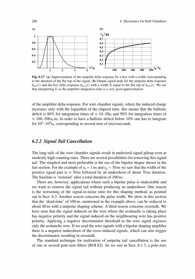
200 6 Electronics for Drift Chambers
1 2 3 4
0.2
0.4
0.6
0.8
1
100 200 300 400 500
0.1
0.2
0.3
0.4
0.5
0.6
0.7
v / gq
tp / t0t / t0
p
(a) (b)
Fig. 6.17 (a) Approximation of the unipolar delta response by a box with a width correspondingto the duration of the flat top of the signal. (b) Output signal peak for the unipolar delta responsehuni(t) and the box delta response hbox(t) with a width TI equal to the flat top of huni(t). We seethat interpreting TI as the amplifier integration time is a very good approximation
of the amplifier delta response. For wire chamber signals, where the induced chargeincreases only with the logarithm of the elapsed time, this means that the ballisticdeficit is 80% for integration times of ≈ 10–20t0 and 50% for integration times of≈ 100–200 t0 ns. In order to have a ballistic deficit below 10% one has to integratefor 103–104t0, corresponding to several tens of microseconds.
6.2.2 Signal Tail Cancellation
The long tails of the wire chamber signals result in undesired signal pileup even atmodestly high counting rates. There are several possibilities for removing this signaltail. The simplest and most preferable is the use of the bipolar shaper shown in thelast section. For the example of t0 = 1ns and tp = 10ns we saw that the width of thepositive signal part is ≈ 30ns followed by an undershoot of about 70 ns duration.The baseline is ‘restored’ after a total duration of 100 ns.
There are, however, applications where such a bipolar pulse is undesirable andwe want to remove the signal tail without producing an undershoot. One reasonis the worsening of the signal-to-noise ratio for this shaping method, as pointedout in Sect. 6.3. Another reason concerns the pulse width. We show in this sectionthat the ‘dead-time’ of 100 ns, mentioned in the example above, can be reduced toabout 40 ns with a unipolar shaping scheme. A third reason concerns crosstalk. Wehave seen that the signal induced on the wire where the avalanche is taking placehas negative polarity and the signal induced on the neighbouring wire has positivepolarity. Applying a negative discriminator threshold to the wire signal registersonly the avalanche wire. If we read the wire signals with a bipolar shaping amplifierthere is a negative undershoot of the cross-induced signals, which can also triggerthe discriminator, resulting in crosstalk.
The standard technique for realization of unipolar tail cancellation is the useof one or several pole-zero filters [BOI 82]. As we saw in Sect. 6.1.3, a pole-zero

6.2 Signal Shaping 201
filter with time constants τ1 and τ2 transforms an exponential signal of the formexp(−t/τ1) into an exponential signal with time constant τ2 (Fig. 6.8). In orderto apply such a procedure to our wire chamber signal we first approximate thesignal
i(t) =q
2t0 ln ba
11+ t/t0
= I01
1+ t/t0(6.45)
by a sum of exponentials with increasing time constants τn = t0/αn:
i(t) � I0
N
∑n=1
An e−αn t/t0 = I0
N
∑n=1
An e−t/τn τn < τn+1. (6.46)
By choosing the number of exponential terms N sufficiently large, the signal can beapproximated to any desired accuracy. The Laplace transform of the above expres-sion is
I(s) = L [i(t)] = I0
N
∑n=1
An
s+1/τn. (6.47)
For illustration we use two exponentials:
i(t) = I0
(A1e−t/τ1 +A2e−t/τ2
)I(s) = I0
(A1
s+1/τ1+
A2
s+1/τ2
)(6.48)
and rewrite the expression as
I(s) = I0(A1 +A2)(s+1/τ1)
(s+1/τ)(s+1/τ2)
τ = τ1τ2A1 +A2
A1τ1 +A2τ2< τ2. (6.49)
Applying a pole-zero filter with the time constants τ2 and τ to the signal, i.e.,WPZ(s) = (s+1/τ2)/(s+1/τ), results in the output signal
I2(s) = I(s)s+1/τ2
s+1/τ= I0
A1 +A2
s+1/τ1i2(t) = I0(A1 +A2)e−t/τ1 , (6.50)
which is a single exponential. This means that applying a pole-zero filter withthese specially chosen time constants to the sum of two exponential signals isequivalent to ‘removing’ one of the exponential terms. The procedure is easily ex-tended to the sum of several exponentials. Representing i(t) by the sum of threeexponentials we need two pole-zero filters to arrive at a single exponential, andfor N exponentials we need N − 1 filters to remove all but the first exponentialterm.
In order to find the constants An and αn = τn/t0 that approximate i(t), we mini-mize the area (charge) between i(t) and the sum of exponentials
∫ kt0
0
(1
1+ t/t0−
N
∑n=1
Ane−αnt/t0
)2
dt → min. (6.51)
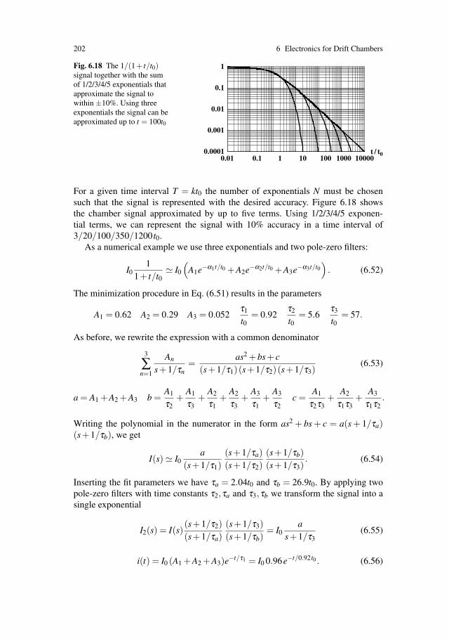
202 6 Electronics for Drift Chambers
Fig. 6.18 The 1/(1+ t/t0)signal together with the sumof 1/2/3/4/5 exponentials thatapproximate the signal towithin ±10%. Using threeexponentials the signal can beapproximated up to t = 100t0
0.01 0.1 1 10 100 1000 100000.0001
0.001
0.01
0.1
1
t / t0
For a given time interval T = kt0 the number of exponentials N must be chosensuch that the signal is represented with the desired accuracy. Figure 6.18 showsthe chamber signal approximated by up to five terms. Using 1/2/3/4/5 exponen-tial terms, we can represent the signal with 10% accuracy in a time interval of3/20/100/350/1200 t0.
As a numerical example we use three exponentials and two pole-zero filters:
I01
1+ t/t0� I0
(A1e−α1t/t0 +A2e−α2t/t0 +A3e−α3t/t0
). (6.52)
The minimization procedure in Eq. (6.51) results in the parameters
A1 = 0.62 A2 = 0.29 A3 = 0.052τ1
t0= 0.92
τ2
t0= 5.6
τ3
t0= 57.
As before, we rewrite the expression with a common denominator
3
∑n=1
An
s+1/τn=
as2 +bs+ c(s+1/τ1)(s+1/τ2)(s+1/τ3)
(6.53)
a = A1 +A2 +A3 b =A1
τ2+
A1
τ3+
A2
τ1+
A2
τ3+
A3
τ1+
A3
τ2c =
A1
τ2τ3+
A2
τ1τ3+
A3
τ1τ2.
Writing the polynomial in the numerator in the form as2 + bs + c = a(s + 1/τa)(s+1/τb), we get
I(s) � I0a
(s+1/τ1)(s+1/τa)(s+1/τ2)
(s+1/τb)(s+1/τ3)
. (6.54)
Inserting the fit parameters we have τa = 2.04t0 and τb = 26.9t0. By applying twopole-zero filters with time constants τ2,τa and τ3,τb we transform the signal into asingle exponential
I2(s) = I(s)(s+1/τ2)(s+1/τa)
(s+1/τ3)(s+1/τb)
= I0a
s+1/τ3(6.55)
i(t) = I0 (A1 +A2 +A3)e−t/τ1 = I0 0.96e−t/0.92 t0 . (6.56)

6.2 Signal Shaping 203
20 40 60 80 1000.2
0.2
0.4
0.6
0.8
1
(a) (b)
200 400 600 800 1000
0.02
0.01
0.01
0.02
t / t0
t / t0
Fig. 6.19 (a) Wire chamber signal processed by a unipolar shaper of n = 4 and tp/t0 = 10 togetherwith the same signal filtered by of two pole-zero filters. The pulse width is reduced to a length ofT � 40t0. (b) The same signal on a smaller vertical scale, showing a tail with a height correspondingto about 1% of the chamber signal
Figure 6.19 shows the result of applying these two pole-zero filters to the wire cham-ber signal of Eq. (6.45), which was processed by a unipolar shaper with n = 4 andtp/t0 = 10. For this purpose we convoluted the signal v(t) from Eq. (6.42) with thedelta response of the pole-zero filter from Eq. (6.25):
v2(t) =∫ t
0wPZ(t − t ′)v(t ′)dt ′ = v(t)−
∫ t
0
τ2 − τa
τ2τae−(t−t ′)/τa v(t ′)dt ′. (6.57)
We see that the result is very satisfactory: the two pole-zero filters have considerablyreduced the signal length to about 40t0 and only a small tail below 1% of the peakvalue remains.
Improvement for Long Peaking Times: In the previous example, two of thefitted exponential time constants were rather small (0.92t0 and 5.6t0) because theyhad to represent the steep part of the original wire signal at very short times. Butfor amplifiers with long peaking times tp � t0, the output pulse shape does notdepend on the exact form of the input at times < tp, but only on the signal chargeduring this time. We can then achieve a closer approximation by first convolutingthe exponential terms with the amplifier response and then fitting this signal to thechamber signal processed by the amplifier. The fit can extend over times as long asseveral hundred t0.
v1(t) = g∫ t
0huni(t − t ′)
I0
1+ t ′/t0dt ′ v2(t) = L −1
[gHuni(s)I0
N
∑m=1
Am
s+1/τm
].
(6.58)
The parameters An,αn in the analytic expression of v2(t) are then determined suchthat the ‘amplified’ signal v1(t) is represented as closely as possible. The analyticrepresentation of v2(t) can be expressed by making use of the relations
L −1[
Huni(s)A
s+1/τ
]= L −1
[tp enn!
(n+ stp)n+1
A(s+1/τ)
]= A f (t,τ)

204 6 Electronics for Drift Chambers
f (t,τ) = tp n!en(
n− tp
τ
)−(n+1)(
e−t/τ − e−nt/tpn
∑m=0
1m!
[(n− tp
τ
) ttp
]m)
.
(6.59)
Thus for three exponentials the signal is expressed as
v2(t) = gI0 (A1 f (t,τ1)+A2 f (t,τ2)+A3 f (t,τ3)) . (6.60)
For a value of tp/t0 = 10, the signal v1(t) is approximated to within ±10% accuracyup to 350t0 by the parameters
A1 = 0.60 A2 = 0.10 A3 = 0.016τ1
t0= 2.48
τ2
t0= 18.8
τ3
t0= 191.
Using two pole-zero filters with these time constants, giving τa = 9.37,τb = 107.35results in the output signal presented in Fig. 6.20. A small bump with a height of0.5% of the peak value is followed by a remaining tail of only 0.25% relative height.This is an improvement of a factor 2 compared to the previous scheme.
Although the unipolar-shaped pulse is shorter and avoids the undershoot, thereare several issues that have to be considered carefully when choosing this shapingscheme. First, one has to evaluate the effects of the remaining signal tail, which lastsup to 105t0 in our example. Although the tail is small, the statistical superpositionof many of them may result in significant baseline fluctuations. In addition, the pre-cise cancellation of the signal tail requires a very good knowledge of the chambersignal shape. Because the time constant t0 depends on the ion mobility and appliedhigh voltage, the signal shape depends on the working point and the gas mixturethat is used. The optimized pole-zero filter constants are therefore in principle onlyvalid for a single well-defined working point. Another word of caution concerns therealization of the pole-zero filters. Resistors and capacitors have certain productionvariations. In integrated circuits, the absolute values of R and C elements have typ-ical errors of up to 10%, so the precise realization of the time constants is ratherdifficult. The tail cancellation effect is mostly defined by the so-called pole/zeroratio τ1/τ2, which itself is determined by the ratio of resistors. Although ratios of
20 40 60 80 1000.2
0.2
0.4
0.6
0.8
1
200 400 600 800 1000
0.015
0.01
0.005
0.005
0.01
0.015
t / t0
t / t0
(a) (b)
Fig. 6.20 (a) Application of the two pole-zero filters to the wire chamber signal, where the pole-zero time constants were determined after processing with the unipolar shaper. (b) The same signalon a smaller vertical scale showing a tail of only 0.25% height

6.2 Signal Shaping 205
resistors on ICs are typically correct to about 1% it is still very tedious to fine-tunethe time constants.
It is therefore advisable to use the bipolar scheme whenever possible owing toits simplicity and insensitivity to working point variations and imprecisions of elec-tronic elements. In the case where unipolar shaping is required for reasons outlinedin the introduction, it is usually essential to make the pole-zero time constants pro-grammable in order to be able to compensate for process variations and adapt tochanging working points.
6.2.3 Signal Pileup, Baseline Shift, and Baseline Fluctuations
At high counting rates, when the time between signals is not long compared tothe signal pulse width, the individual signals pile up and cause a deterioration ofthe signal quality. This can be calculated if one uses the fact that the individualpulses come at random and therefore have an exponential distribution of the timeinterval between any two consecutive signals. The probability P(t)dt for finding atime interval t, t +dt is
P(t)dt =1τ
e−t/τ dt = νe−νt dt, (6.61)
where ν is the average pulse rate and τ = 1/ν is the average time between twoconsecutive pulses. The effect of different pulse shapes at high counting rates isdemonstrated in the four parts of Fig. 6.21, where we see a rapid random sequenceof identical pulses treated by four different shapers. We use the remainder of thissection to quantify what we see. The rate ν is taken to be ν = 5× 10⁻³/t0, whichcorresponds to 5 MHz when t0 = 1 ns.
For the following discussion it is useful to separate the signal into a ‘signal’part of duration T and a ‘tail’ part (Fig. 6.22). The first high-rate effect to discuss issignal pileup, where the ‘signal’ part of two signals arrives within a time interval thatis smaller than the signal pulse width T . This pileup results in incorrect charge ortime measurement. In a particle tracking system, the particle trajectory is typicallymeasured by several readout channels, and the track reconstruction can detect thechannel with incorrect charge or time measurement. Consequently the measurementfrom this channel is not used in the reconstruction, which results in an inefficiencyof this channel. The signal pileup probability, or inefficiency ε , for a pulse width Tand a rate ν is given by
ε =∫ T
0νe−νt dt = 1− e−νT ≈ T
τfor T τ . (6.62)
The rate requirement is therefore one key element for specification of the maximumpulse width T , which in turn specifies the shaping strategy. The signal part of thebipolar pulse in Fig. 6.16a has a duration of T ≈ 80t0 while the signal part of the
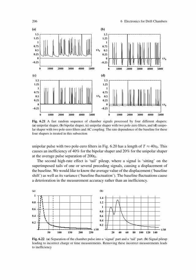
206 6 Electronics for Drift Chambers
0 1000 2000 3000 4000 5000
–0.250
0.250.5
0.751
1.251.5
(a) (b)
(c) (d)
0 1000 2000 3000 4000 5000
00.25
0.50.75
11.25
1.5
0 1000 2000 3000 4000 5000
0
0.250.5
0.751
1.251.5
t/t0
t/t0
0 1000 2000 3000 4000 5000
–0.25 –0.250
0.250.5
0.751
1.251.5
t/t0
–0.25t/t0
Fig. 6.21 A fast random sequence of chamber signals processed by four different shapers:(a) unipolar shaper, (b) bipolar shaper, (c) unipolar shaper with two pole-zero filters, and (d) unipo-lar shaper with two pole-zero filters and AC coupling. The rate dependence of the baseline for thesefour shapers is treated in this subsection
unipolar pulse with two pole-zero filters in Fig. 6.20 has a length of T ≈ 40 t0. Thiscauses an inefficiency of 40% for the bipolar shaper and 20% for the unipolar shaperat the average pulse separation of 200t0.
The second high-rate effect is ‘tail’ pileup, where a signal is ‘sitting’ on thesuperimposed tails of one or several preceding signals, causing a displacement ofthe baseline. We would like to know the average value of the displacement (‘baselineshift’) as well as its variance (‘baseline fluctuation’). The baseline fluctuations causea deterioration in the measurement accuracy rather than an inefficiency.
50 100 150 200 250t /t0 t /t0
0.2
0.4
0.6
0.8
(a) (b)
1
20 40 60 80 100 120 140
0.2
0.4
0.6
0.8
1
1.2
1.4
Fig. 6.22 (a) Separation of the chamber pulse into a ‘signal’ part and a ‘tail’ part. (b) Signal pileupleading to incorrect charge or time measurements. Removing these incorrect measurements leadsto inefficiency
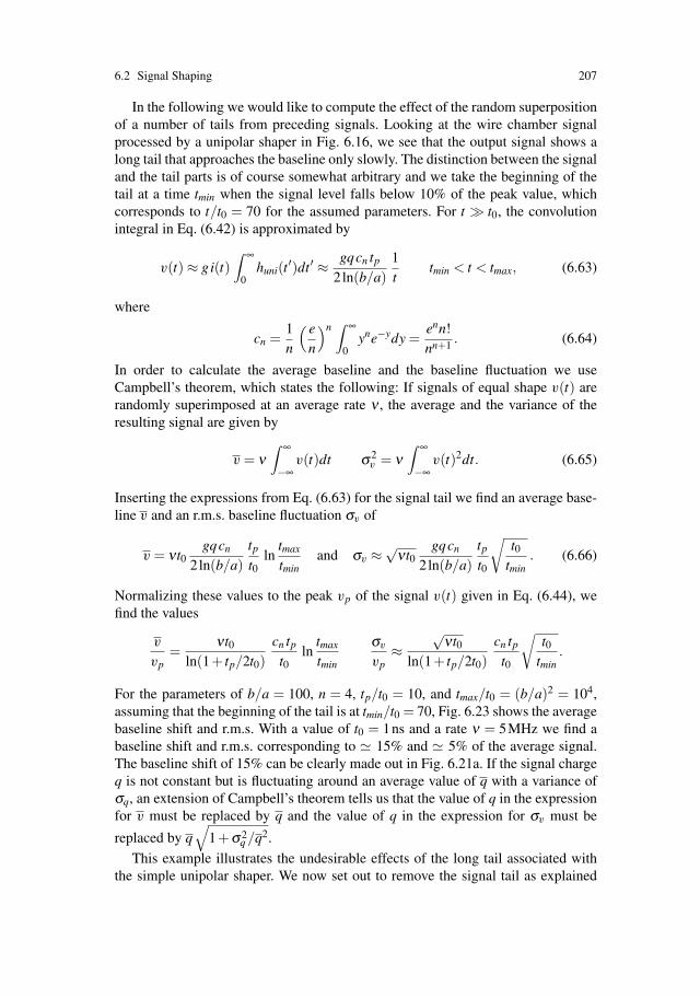
6.2 Signal Shaping 207
In the following we would like to compute the effect of the random superpositionof a number of tails from preceding signals. Looking at the wire chamber signalprocessed by a unipolar shaper in Fig. 6.16, we see that the output signal shows along tail that approaches the baseline only slowly. The distinction between the signaland the tail parts is of course somewhat arbitrary and we take the beginning of thetail at a time tmin when the signal level falls below 10% of the peak value, whichcorresponds to t/t0 = 70 for the assumed parameters. For t � t0, the convolutionintegral in Eq. (6.42) is approximated by
v(t) ≈ gi(t)∫ ∞
0huni(t ′)dt ′ ≈ gqcn tp
2ln(b/a)1t
tmin < t < tmax, (6.63)
where
cn =1n
( en
)n ∫ ∞
0yne−ydy =
enn!nn+1 . (6.64)
In order to calculate the average baseline and the baseline fluctuation we useCampbell’s theorem, which states the following: If signals of equal shape v(t) arerandomly superimposed at an average rate ν , the average and the variance of theresulting signal are given by
v = ν∫ ∞
−∞v(t)dt σ2
v = ν∫ ∞
−∞v(t)2dt. (6.65)
Inserting the expressions from Eq. (6.63) for the signal tail we find an average base-line v and an r.m.s. baseline fluctuation σv of
v = νt0gqcn
2ln(b/a)tp
t0ln
tmax
tminand σv ≈
√νt0
gqcn
2ln(b/a)tp
t0
√t0
tmin. (6.66)
Normalizing these values to the peak vp of the signal v(t) given in Eq. (6.44), wefind the values
v
vp=
νt0ln(1+ tp/2t0)
cn tp
t0ln
tmax
tmin
σv
vp≈
√νt0
ln(1+ tp/2t0)cn tp
t0
√t0
tmin.
For the parameters of b/a = 100, n = 4, tp/t0 = 10, and tmax/t0 = (b/a)2 = 104,assuming that the beginning of the tail is at tmin/t0 = 70, Fig. 6.23 shows the averagebaseline shift and r.m.s. With a value of t0 = 1ns and a rate ν = 5MHz we find abaseline shift and r.m.s. corresponding to � 15% and � 5% of the average signal.The baseline shift of 15% can be clearly made out in Fig. 6.21a. If the signal chargeq is not constant but is fluctuating around an average value of q with a variance ofσq, an extension of Campbell’s theorem tells us that the value of q in the expressionfor v must be replaced by q and the value of q in the expression for σv must be
replaced by q√
1+σ2q /q2.
This example illustrates the undesirable effects of the long tail associated withthe simple unipolar shaper. We now set out to remove the signal tail as explained

208 6 Electronics for Drift Chambers
1 2 3 4 5–5
5
10
15
20
unipolar
unipolar/2PZ
unipolar/2PZ/CR1 2 3 4 5
1
2
3
4
5
6
unipolar
unipolar/2PZ+RCν t0 10–3
σv /vp%v/vp%
_(a) (b)
–10 ν t0 10–3
Fig. 6.23 Average baseline shift (a) and baseline fluctuation (b) for various shapers, as a functionof the signal rate ν
in the previous section. Let us apply two pole-zero filters with time constants τ2,τa
and τ3,τb, which remove the signal tail up to ≈ 3τ3. For times longer than 3τ3 thepole-zero filters are just scaling the signal without changing the shape, because thetransfer is then approximately constant,
iω +1/τ2
iω +1/τa
iω +1/τ3
iω +1/τb≈ τa
τ2
τb
τ3for ω 1
τ3. (6.67)
The signal tail is therefore given by the expression from Eq. (6.63) scaled by thisfactor:
v(t) ≈ gqcn tp
2ln(b/a)τa
τ2
τb
τ3
1t
3τ3 < t < tmax. (6.68)
The expressions for the average and r.m.s of the baseline are equal those fromEq. (6.66), scaled by τaτb/τ2τ3 with tmin replaced by 3τ3.
In order to express the baseline shift and fluctuation as a fraction of the pulseheight we must first find the peak of the unipolar-shaped signal processed by twopole-zero filters. We use the fact that the pole-zero filters remove all but the first ex-ponential, so the remaining signal is given by i(t) = Aexp(−tτ1) [Eq. (6.56)], wherewe have defined A = A1 + A2 + A3. The procedure for determining the pole-zeroparameters results in a time constant τ1 which is much smaller than the amplifierpeaking time tp, so we can assume that the entire signal charge is contained in adelta signal and find the amplifier output peak vp:
vp = gQ = g∫ ∞
0i(t)dt =
gq
2t0 ln ba
Aτ1. (6.69)
Thus, the average baseline shift and the r.m.s. fluctuation are
v
vp= νt0
cn
A
tpτaτb
τ1τ2τ3ln
tmax
3τ3
σv
vp≈√
νt0cn
A
tpτaτb
τ1τ2τ3
√t0
3τ3.
Figure 6.23 shows the results using the time constants that we determined in theprevious section. With t0 = 1 ns at a rate of 5 MHz we find a baseline shift of 3%and a baseline fluctuation of 0.8% of the average pulse height. In Fig. 6.21c we see
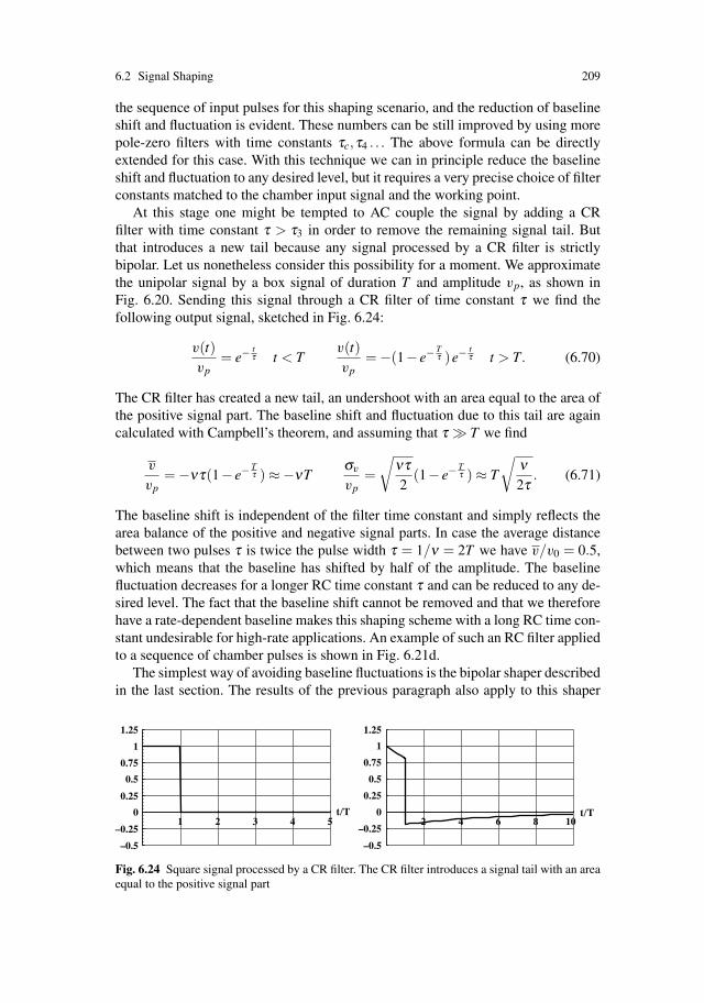
6.2 Signal Shaping 209
the sequence of input pulses for this shaping scenario, and the reduction of baselineshift and fluctuation is evident. These numbers can be still improved by using morepole-zero filters with time constants τc,τ4 . . . The above formula can be directlyextended for this case. With this technique we can in principle reduce the baselineshift and fluctuation to any desired level, but it requires a very precise choice of filterconstants matched to the chamber input signal and the working point.
At this stage one might be tempted to AC couple the signal by adding a CRfilter with time constant τ > τ3 in order to remove the remaining signal tail. Butthat introduces a new tail because any signal processed by a CR filter is strictlybipolar. Let us nonetheless consider this possibility for a moment. We approximatethe unipolar signal by a box signal of duration T and amplitude vp, as shown inFig. 6.20. Sending this signal through a CR filter of time constant τ we find thefollowing output signal, sketched in Fig. 6.24:
v(t)vp
= e−tτ t < T
v(t)vp
= −(1− e−Tτ )e−
tτ t > T. (6.70)
The CR filter has created a new tail, an undershoot with an area equal to the area ofthe positive signal part. The baseline shift and fluctuation due to this tail are againcalculated with Campbell’s theorem, and assuming that τ � T we find
v
vp= −ντ(1− e−
Tτ ) ≈−νT
σv
vp=√
ντ2
(1− e−Tτ ) ≈ T
√ν2τ
. (6.71)
The baseline shift is independent of the filter time constant and simply reflects thearea balance of the positive and negative signal parts. In case the average distancebetween two pulses τ is twice the pulse width τ = 1/ν = 2T we have v/v0 = 0.5,which means that the baseline has shifted by half of the amplitude. The baselinefluctuation decreases for a longer RC time constant τ and can be reduced to any de-sired level. The fact that the baseline shift cannot be removed and that we thereforehave a rate-dependent baseline makes this shaping scheme with a long RC time con-stant undesirable for high-rate applications. An example of such an RC filter appliedto a sequence of chamber pulses is shown in Fig. 6.21d.
The simplest way of avoiding baseline fluctuations is the bipolar shaper describedin the last section. The results of the previous paragraph also apply to this shaper
1 2 3 4 5t/T
0.25
0.5
0.75
1
1.25
02 4 6 8 10
–0.5
–0.25
–0.5
–0.25
0.25
0.5
0.75
1
1.25
0 t/T
Fig. 6.24 Square signal processed by a CR filter. The CR filter introduces a signal tail with an areaequal to the positive signal part

210 6 Electronics for Drift Chambers
because the bipolar shaper is equal to a unipolar shaper with an additional CR fil-ter. But now the CR time constant is short—of the same order as the signal lengthT —so this shaper creates a large, but short undershoot. The area balance is done‘quickly’, and after a duration of two to three times tp the signal is back to thebaseline.
The tail of the output of the bipolar shaper is found by writing the output signalin the Laplace domain and interpreting the s in the numerator as the derivative ofthe unipolar output signal:
v(t) = L −1 [gHbip(s)I(s)]= g
ddt
L −1[
1s
Hbip(s)I(s)]≈ gi′(t) lim
s→0
1s
Hbip(s)
(6.72)
v(t) ≈−gqern!√nrn+1
12ln(b/a)
t2p
t2 . (6.73)
We see that the negative signal tail tends to zero as 1/t2, which guarantees a quickreturn to the baseline, and the influence on the following pulses is eliminated. Theeffect of this shaping scheme is shown in Fig. 6.21b. It can be seen that the pulsewidth and therefore the inefficiency is increased, but the baseline is equal to zeroand the fluctuations are eliminated.
Conclusion of this Section
There are two linear signal processing strategies by which we can avoid baselineshift and baseline fluctuations at high counting rates owing to the long tail of wirechamber signals:
Unipolar Shaping: A unipolar shaper and several pole-zero filters matched tothe individual exponentials that represent the chamber signal are used. The advan-tage is a ‘short’ unipolar response. There are, however, several disadvantages to thisapproach. First of all, the entire electronics readout chain must be DC coupled. Thiscauses problems for the electronics design because the DC offset variations withinthe electronics chain, which are due to component imperfections or temperaturevariations, must be very carefully controlled. The DC coupling also makes the elec-tronics sensitive to low-frequency noise, which is very undesirable. In addition, thewire signals are intrinsically AC coupled owing to the capacitor that decouples thewire high voltage from the amplifier input, so a unipolar shaping strategy is simplynot realizable with a linear electronics circuit. In addition, the pole-zero parametersmust be carefully tuned to the signal tail constant t0, which depends on the chambergeometry, the gas used, and even the operating voltage. Since the absolute values ofresistors and capacitors in most electronics technologies can vary by 10–20% withrespect to the nominal values, the needed precision of the achieved time constantsmust be very carefully evaluated. A solution to this problem is the introduction ofprogrammable pole-zero time constants, but this, of course, adds another level ofcomplication.
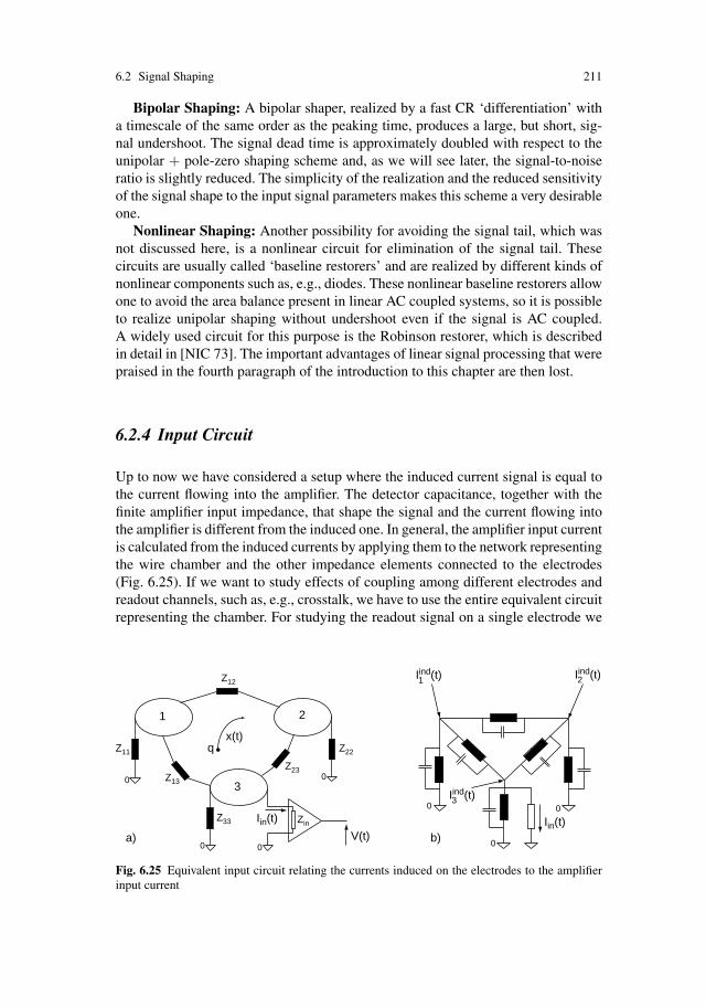
6.2 Signal Shaping 211
Bipolar Shaping: A bipolar shaper, realized by a fast CR ‘differentiation’ witha timescale of the same order as the peaking time, produces a large, but short, sig-nal undershoot. The signal dead time is approximately doubled with respect to theunipolar + pole-zero shaping scheme and, as we will see later, the signal-to-noiseratio is slightly reduced. The simplicity of the realization and the reduced sensitivityof the signal shape to the input signal parameters makes this scheme a very desirableone.
Nonlinear Shaping: Another possibility for avoiding the signal tail, which wasnot discussed here, is a nonlinear circuit for elimination of the signal tail. Thesecircuits are usually called ‘baseline restorers’ and are realized by different kinds ofnonlinear components such as, e.g., diodes. These nonlinear baseline restorers allowone to avoid the area balance present in linear AC coupled systems, so it is possibleto realize unipolar shaping without undershoot even if the signal is AC coupled.A widely used circuit for this purpose is the Robinson restorer, which is describedin detail in [NIC 73]. The important advantages of linear signal processing that werepraised in the fourth paragraph of the introduction to this chapter are then lost.
6.2.4 Input Circuit
Up to now we have considered a setup where the induced current signal is equal tothe current flowing into the amplifier. The detector capacitance, together with thefinite amplifier input impedance, that shape the signal and the current flowing intothe amplifier is different from the induced one. In general, the amplifier input currentis calculated from the induced currents by applying them to the network representingthe wire chamber and the other impedance elements connected to the electrodes(Fig. 6.25). If we want to study effects of coupling among different electrodes andreadout channels, such as, e.g., crosstalk, we have to use the entire equivalent circuitrepresenting the chamber. For studying the readout signal on a single electrode we
00
0
qx(t)
0
0
0
Z11
a) b)
Iind(t)1
Iin(t)
0
Zin
V(t)
1
3
2
Z13
Z33
Z23
Z22
Z12Iind(t)2
Iind(t)3
Iin(t)
Fig. 6.25 Equivalent input circuit relating the currents induced on the electrodes to the amplifierinput current
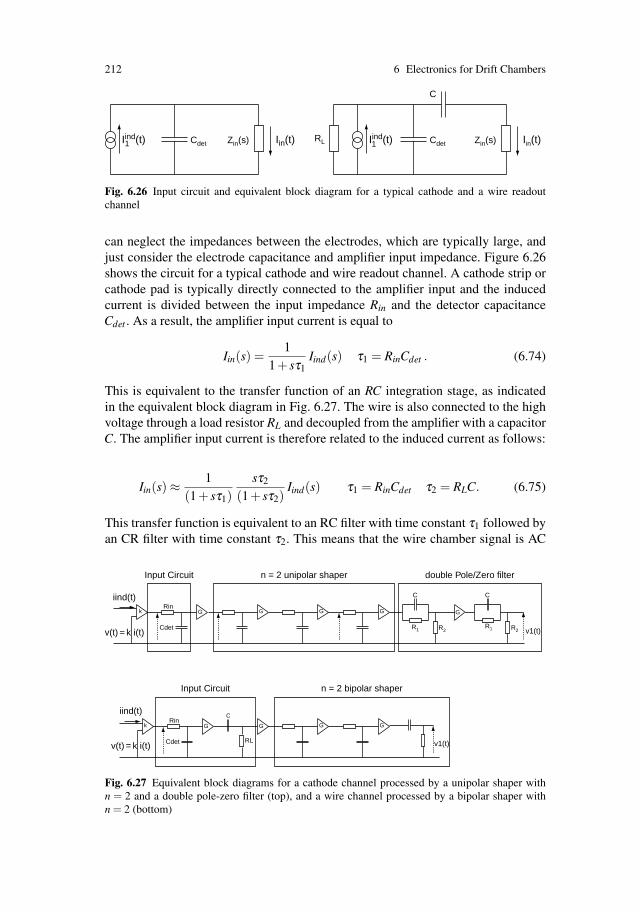
212 6 Electronics for Drift Chambers
C
Zin(s)RL CdetIind(t) Iin(t)Zin(s)CdetIind(t)1 Iin(t) 1
Fig. 6.26 Input circuit and equivalent block diagram for a typical cathode and a wire readoutchannel
can neglect the impedances between the electrodes, which are typically large, andjust consider the electrode capacitance and amplifier input impedance. Figure 6.26shows the circuit for a typical cathode and wire readout channel. A cathode strip orcathode pad is typically directly connected to the amplifier input and the inducedcurrent is divided between the input impedance Rin and the detector capacitanceCdet . As a result, the amplifier input current is equal to
Iin(s) =1
1+ sτ1Iind(s) τ1 = RinCdet . (6.74)
This is equivalent to the transfer function of an RC integration stage, as indicatedin the equivalent block diagram in Fig. 6.27. The wire is also connected to the highvoltage through a load resistor RL and decoupled from the amplifier with a capacitorC. The amplifier input current is therefore related to the induced current as follows:
Iin(s) ≈1
(1+ sτ1)sτ2
(1+ sτ2)Iind(s) τ1 = RinCdet τ2 = RLC. (6.75)
This transfer function is equivalent to an RC filter with time constant τ1 followed byan CR filter with time constant τ2. This means that the wire chamber signal is AC
iind(t)
v(t) = k i(t)
v1(t)
v1(t)
iind(t)
v(t) = k i(t)
C
Rin
Cdet
Gk
R1
C C
GG G G
Rin
Cdet
Gk G G G
RL
Input Circuit
Input Circuit
n = 2 unipolar shaper
n = 2 bipolar shaper
double Pole/Zero filter
R2R1 R2
Fig. 6.27 Equivalent block diagrams for a cathode channel processed by a unipolar shaper withn = 2 and a double pole-zero filter (top), and a wire channel processed by a bipolar shaper withn = 2 (bottom)

6.3 Noise and Optimum Filters 213
coupled and the output signal of any linear signal processing chain connected to thewire is strictly bipolar.
The current signal Iin(s) is then processed by the readout electronics chain.Figure 6.27 shows how the input circuit is represented in an equivalent blockdiagram. The examples show a cathode signal processed by a unipolar shaper withtwo pole-zero filters and a wire signal processed by a bipolar shaper. The amplifieroutput signals for the two scenarios are given by
V (s) =1
1+ sRinCdet
G(1+ sτ)n+1
s+1/τ1
s+1/τa
s+1/τ2
s+1/τbIind(s), (6.76)
V (s) =1
1+ sRinCdet
sRLC(1+ sRLC)
Gsτ(1+ sτ)n+1 Iind(s). (6.77)
6.3 Noise and Optimum Filters
By this point we are familiar with various possible transfer functions and pulseshapes for analyzing wire chamber signals so that for a given application we have achoice for achieving the best performance. There is one more element which oftenplays an essential role when designing optimal chamber electronics—the inevitablenoise present in all electronics elements as well as in the wire chamber itself, whichrepresents a background against which the signals have to be distinguished. In thefollowing sections we characterize noise as a general phenomenon, discuss somerelevant noise sources, and develop a method for studying the influence of the noisesource on the signal pulse shapes. In the end we want to find the optimum transferfunction for a given application.
For optimum charge measurement in cathode pad and cathode strip chambers, thenoise may limit the measurement accuracy and we want to choose H(iω) such thatthe signal-to-noise ratio is maximized. The choice of H(iω) for time measurementis more complicated. The time resolution of a wire chamber is determined by thechamber internal effects of primary ionization and electron dynamics together withthe electronics noise. In order to minimize the noise effect one has to maximize theso-called ‘slope-to-noise’ ratio, which may sometimes pose conditions unfavourablefor exploiting the measurement accuracy of the chamber itself.
In principle the signal-to-noise ratio and slope to noise ratio can always beimproved by increasing the chamber gas gain. On the other hand, for reasons ofchamber ageing and rate limitations, one wants to work at the lowest possible gasgain.
The ‘optimum filters’ that minimize the effect of noise are related in a unique wayto the input signal shape and the noise spectrum, but they are not always realizableor practical. They serve as a guideline for choosing the parameters for a realisticdesign and show how far it deviates from the theoretically optimal performance.The optimum filter might result in a very long pulse which is not compatible withrate requirements or it might increase the impact of the chamber internal effects.
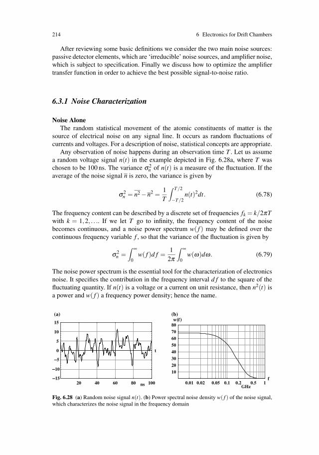
214 6 Electronics for Drift Chambers
After reviewing some basic definitions we consider the two main noise sources:passive detector elements, which are ‘irreducible’ noise sources, and amplifier noise,which is subject to specification. Finally we discuss how to optimize the amplifiertransfer function in order to achieve the best possible signal-to-noise ratio.
6.3.1 Noise Characterization
Noise AloneThe random statistical movement of the atomic constituents of matter is the
source of electrical noise on any signal line. It occurs as random fluctuations ofcurrents and voltages. For a description of noise, statistical concepts are appropriate.
Any observation of noise happens during an observation time T . Let us assumea random voltage signal n(t) in the example depicted in Fig. 6.28a, where T waschosen to be 100 ns. The variance σ2
n of n(t) is a measure of the fluctuation. If theaverage of the noise signal n is zero, the variance is given by
σ2n = n2 −n2 =
1T
∫ T/2
−T/2n(t)2dt. (6.78)
The frequency content can be described by a discrete set of frequencies fk = k/2πTwith k = 1,2, . . .. If we let T go to infinity, the frequency content of the noisebecomes continuous, and a noise power spectrum w( f ) may be defined over thecontinuous frequency variable f , so that the variance of the fluctuation is given by
σ2n =
∫ ∞
0w( f )d f =
12π
∫ ∞
0w(ω)dω. (6.79)
The noise power spectrum is the essential tool for the characterization of electronicsnoise. It specifies the contribution in the frequency interval d f to the square of thefluctuating quantity. If n(t) is a voltage or a current on unit resistance, then n2(t) isa power and w( f ) a frequency power density; hence the name.
20 40 60 80 100
0
5
10
15
t
0.01 0.02 0.05 0.1 0.2 0.5 1f
1020304050607080w f
–5
–10
–15
( )
GHzns
(a) (b)
Fig. 6.28 (a) Random noise signal n(t). (b) Power spectral noise density w( f ) of the noise signal,which characterizes the noise signal in the frequency domain

6.3 Noise and Optimum Filters 215
The noise power spectrum must obviously be related to the Fourier componentsof n(t). The relationship is as follows: If the Fourier transformation is
n(t) =1
2π
∫ ∞
−∞N(iω)eiωt dω, (6.80)
then, using (6.78) and N∗(−iω) = N(ω) and going to the limit, σ2n becomes
limT→∞
2T
∫ T
0|N(iω)|2dω, (6.81)
which implies
w( f ) = limT→∞
2T|N(iω)|2. (6.82)
As an illustration, a typical power spectrum w( f ) has been defined to be flat up to acutoff frequency at 150 MHz, together with an example of a fluctuating voltage n(t)containing frequencies according to w( f ). Both quantities are depicted in Fig. 6.28.The higher this cutoff the more ‘spiky’ the noise.
In the case where the noise power spectrum is constant for all frequencies we callthe noise ‘white’ because the noise signal contains all frequencies in equal amounts.The power spectrum w( f ) is not only useful for calculation of the r.m.s. fluctuationof the noise signal, but it is also related to some other key parameters which charac-terize a noise signal. As was shown by Rice [RIC 44] the average frequency of zerocrossings of n(t) is given by
fzero = 2
√∫ ∞0 f 2 w( f )d f∫ ∞
0 w( f )d f. (6.83)
The evaluation of Eq. (6.83) using the noise power spectrum in Fig. 6.28b givesfzero = 0.31GHz and the noise signal in Fig. 6.28a counts 27 zero crossings in100 ns, giving a rate of 0.27 GHz. For a noise spectrum that is constant up to asharp cutoff frequency f0 this expression evaluates to fzero = 2/
√3 f0 = 1.155 f0.
The frequency of zero crossings of the noise signal is therefore approximately givenby the cutoff frequency of the power spectrum.
Noise in a Linear Network
Now we want to find out how the spectral density of a noise signal is transformedif it is sent through a linear network with transfer function H(iω). The noise sig-nal N(iω) is transformed into N(iω)H(iω). Using Eq. (6.82), we see that the noisepower spectrum is transformed into
w( f ) → w( f )|H(i2π f )|2. (6.84)

216 6 Electronics for Drift Chambers
If we assume a noise signal with a constant power spectrum up to a given frequency,i.e., w( f ) = w0 for f < f0, we find a noise r.m.s. of σn =
√w0 f0. If we send this
noise signal through a low-pass filter of unity gain with a sharp cutoff frequencyf1 < f0, the noise r.m.s. becomes σn =
√w0 f1, meaning that the r.m.s. is reduced
by a factor√
f1/ f0. As shown later one can improve the signal-to-noise ratio byfilters that are passing only the frequencies contained in the signal and removing theothers.
Next we want to find the noise power spectrum at a given circuit node of a linearnetwork in the case where there are several independent (uncorrelated) current andvoltage noise sources distributed throughout the network. Elementary circuit theorytells us that for a set of voltage and current sources distributed in a linear network,the voltage on a given circuit node can be calculated in the following way: Thecontribution of each individual source is computed separately by ‘switching all othersources off’. A source is ‘switched off’ by shorting it out if it is a voltage sourceand by opening it if it is a current source. The final voltage is then the sum of theseindividual contributions. For the network in Fig. 6.29a, e.g., the voltage at nodeV1(s) due to the voltage source V (s) and current source I(s) is
V1(s) =Z2(s)
Z1(s)+Z2(s)V (s)+
Z1(s)Z2(s)Z1(s)+Z2(s)
I(s) . (6.85)
If these are noise sources with voltage noise power spectrum wv( f ) and currentnoise power spectrum wi( f ), Eq. (6.84) tells us that the noise power spectrumwv1( f ) is given by
wv1( f ) =∣∣∣∣ Z2(iω)Z1(iω)+Z2(iω)
∣∣∣∣2
wv( f )+∣∣∣∣ Z1(iω)Z2(iω)Z1(iω)+Z2(iω)
∣∣∣∣2
wi( f ). (6.86)
In order to characterize the signal, noise, and impedance of a wire chamber electrodeconnected to the input of an amplifier, it is very useful to further simplify the pictureby using Thevenin’s and Norton’s theorems (Fig. 6.30):
A linear, active network which contains one or more voltage or current sourcescan be replaced by a single impedance Z(s) with a series voltage source VT (s)(Thevenin’s theorem), or by the same impedance with a parallel current source IN(s)(Norton’s theorem).
The impedance Z(s) can be obtained by shorting out the voltage sources, open-ing up all current sources, and finding the equivalent impedance of the network.The Theveninn equivalent voltage VT (s) or Norton equivalent current IN(s) can be
Z1(s) Z2(s)I(s) V1(s)
V(s)
a) b)
Z2(s) wv1(f)
wv(f)
wi(f)Z1(s)
Fig. 6.29 A voltage source and a current source embedded in a linear network

6.3 Noise and Optimum Filters 217
Z(s)
VT(s)
V(s) Z(s) V(s) = Z(s)I(s)IN(s)V(s)
LinearActive
Network
Fig. 6.30 Illustration of Thevenin’s and Norton’s theorems
calculated by the well known network rules. The voltage VT (s) and current IN(s)are related by VT (s) = Z(s)IN(s). As an example we use the circuit of Fig. 6.29.By shorting the voltage source and opening the current source, the impedanceof the entire network becomes Z(s) = Z1(s)Z2(s)/(Z1(s) + Z2(s)). The Theveninequivalent voltage is given by V1(s) from Eq. (6.85) and the current is thereforeI1(s) = V (s)/Z(s) = I(s)+V (s)/Z(s). The same is true for noise sources: the entirenetwork can again be represented by a single impedance Z(s) with a series volt-age noise power spectrum wv( f ) or a parallel current noise power spectrum wi( f )(Fig. 6.31), and the two are related by
wv( f ) = |Z(i2π f )|2 wi( f ) . (6.87)
Thus we can represent the wire chamber electrode connected to an amplifierinput by a single impedance element Z(s) with a parallel current source representingthe chamber signal and a parallel current noise power spectrum representing allelectrode noise sources (Fig. 6.32).
In this way we can evaluate the relative magnitudes of signal and noise at theamplifier input, which allows us to choose the amplifier transfer function in order tooptimize the signal-to-noise ratio at the amplifier output.
6.3.2 Noise Sources
Having the vocabulary and the tools for noise analysis at hand we can now discussthe different noise sources in a wire chamber setup. We consider only the noise in-herent in the detector and the amplifier and not external ‘man-made’ noise that mayoriginate in various electrical devices outside of the detector. Of course, any suchinterference noise has to be eliminated before approaching the inherent ‘irreducible’detector and amplifier noise.
Z(s)
wv(f)
wv(f) Z(s)wv(f)=wi(f)
LinearNetwork
with noisesources
wv(f) |Z(i2πf)|2 wi(f)
Fig. 6.31 Thevenin’s and Norton’s theorems applied to the noise power spectra

218 6 Electronics for Drift Chambers
Z(s) wi(f) I(s)
Fig. 6.32 Representation of the wire chamber elements, noise sources, and the chamber signal bya single impedance Z(s) with a single current source and a single noise power spectrum
There are many physical processes that create noise in electric circuits. The threemost important ones for particle detection are shot noise, thermal (Johnson) noise,and flicker (1/ f ) noise.
Shot Noise
This electrical noise is based on the random arrival of the smallest quantized unitsof electric charge. The name derives from an analogy with the pellets of a shotgun.If the random sequence is governed by the arrival probability p per unit of timealone (no correlations) one easily calculates the mean number m of particles in anobservation time T as well as the variance, m2 −m2:
m = pT (6.88)
The actual integer number m is distributed around this mean according to the Pois-son probability distribution
P(m,m) =mm
m!e−m. (6.89)
The expectation value of m2 is therefore
∞
∑m=0
m2 mm
m!e−m = m+m2. (6.90)
It follows that the variance is equal to the mean, a famous property of the Poissondistribution. A power spectrum for this kind of noise exists once an electrical pulsee0 f (t) is associated with each noise particle carrying the elementary charge e0. Wehave a random sequence of identical current pulses coming at a mean frequency ν .Campbell’s theorem applies [RIC 44]. It states that under these circumstances theaverage current I and its variance σ2
I are given by
I = ν e0
∫ ∞
−∞f (t)dt σ2
I = ν e20
∫ ∞
−∞f (t)2dt. (6.91)
Applying Parseval’s theorem we can transform the expression for σI into
σ2I = 2νe2
0
∫ ∞
0|F(iω)|2 d f . (6.92)
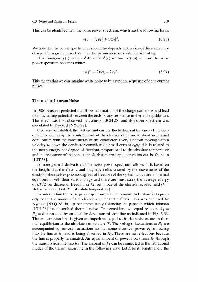
6.3 Noise and Optimum Filters 219
This can be identified with the noise power spectrum, which has the following form:
w( f ) = 2νe20|F(iω)|2. (6.93)
We note that the power spectrum of shot noise depends on the size of the elementarycharge. For a given current νe0 the fluctuation increases with the size of e0.
If we imagine f (t) to be a δ -function δ (t) we have F(iω) = 1 and the noisepower spectrum becomes white:
w( f ) = 2νe20 = 2e0I. (6.94)
This means that we can imagine white noise to be a random sequence of delta currentpulses.
Thermal or Johnson Noise
In 1906 Einstein predicted that Brownian motion of the charge carriers would leadto a fluctuating potential between the ends of any resistance in thermal equilibrium.The effect was first observed by Johnson [JOH 28] and its power spectrum wascalculated by Nyquist [NYQ 28].
One way to establish the voltage and current fluctuations at the ends of the con-ductor is to sum up the contributions of the electrons that move about in thermalequilibrium with the constituents of the conductor. Every electron moving with avelocity ui down the conductor contributes a small current e0ui; this is related tothe mean energy per degree of freedom, proportional to the absolute temperatureand the resistance of the conductor. Such a microscopic derivation can be found in[KIT 58].
A more general derivation of the noise power spectrum follows. It is based onthe insight that the electric and magnetic fields created by the movements of theelectrons themselves possess degrees of freedom of the system which are in thermalequilibrium with their surroundings and therefore must carry the average energyof kT/2 per degree of freedom or kT per mode of the electromagnetic field (k =Boltzmann constant, T = absolute temperature).
In order to find the noise power spectrum, all that remains to be done is to prop-erly count the modes of the electric and magnetic fields. This was achieved byNyquist [NYQ 28] in a paper immediately following the paper in which Johnson[JOH 28] first described thermal noise. One considers two equal resistors R1 =R2 = R connected by an ideal lossless transmission line as indicated in Fig. 6.33.The transmission line is given an impedance equal to R, the resistors are in ther-mal equilibrium at the absolute temperature T . The voltage fluctuations at R1 areaccompanied by current fluctuations so that some electrical power P1 is flowinginto the line at R1 and is being absorbed in R2. There are no reflections becausethe line is properly terminated. An equal amount of power flows from R2 throughthe transmission line into R1. The amount of P1 can be connected to the vibrationalmodes of the transmission line in the following way: Let L be its length and c the
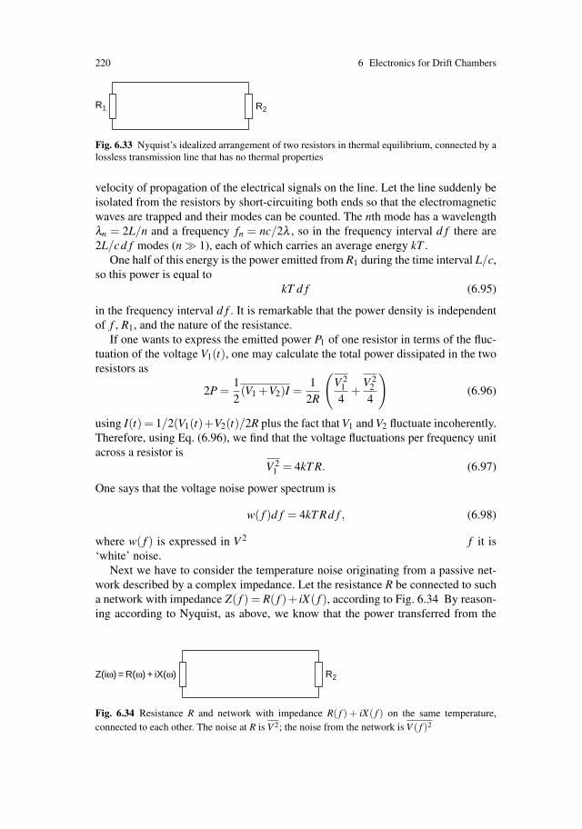
220 6 Electronics for Drift Chambers
R1 R2
Fig. 6.33 Nyquist’s idealized arrangement of two resistors in thermal equilibrium, connected by alossless transmission line that has no thermal properties
velocity of propagation of the electrical signals on the line. Let the line suddenly beisolated from the resistors by short-circuiting both ends so that the electromagneticwaves are trapped and their modes can be counted. The nth mode has a wavelengthλn = 2L/n and a frequency fn = nc/2λ , so in the frequency interval d f there are2L/cd f modes (n � 1), each of which carries an average energy kT .
One half of this energy is the power emitted from R1 during the time interval L/c,so this power is equal to
kT d f (6.95)
in the frequency interval d f . It is remarkable that the power density is independentof f , R1, and the nature of the resistance.
If one wants to express the emitted power P1 of one resistor in terms of the fluc-tuation of the voltage V1(t), one may calculate the total power dissipated in the tworesistors as
2P =12(V1 +V2)I =
12R
(V 2
1
4+
V 22
4
)(6.96)
using I(t) = 1/2(V1(t)+V2(t)/2R plus the fact that V1 and V2 fluctuate incoherently.Therefore, using Eq. (6.96), we find that the voltage fluctuations per frequency unitacross a resistor is
V 21 = 4kT R. (6.97)
One says that the voltage noise power spectrum is
w( f )d f = 4kT Rd f , (6.98)
where w( f ) is expressed in V 2/Hz [cf. Eq. (6.79)]. As it is independent of f it is‘white’ noise.
Next we have to consider the temperature noise originating from a passive net-work described by a complex impedance. Let the resistance R be connected to sucha network with impedance Z( f ) = R( f )+ iX( f ), according to Fig. 6.34 By reason-ing according to Nyquist, as above, we know that the power transferred from the
R2Z(iω) = R(ω) + iX(ω)
Fig. 6.34 Resistance R and network with impedance R( f ) + iX( f ) on the same temperature,connected to each other. The noise at R is V 2; the noise from the network is V ( f )2

6.3 Noise and Optimum Filters 221
resistance to the network is equal to that transferred in the opposite direction. Theformer is seen by simple circuit theory to be equal to
V 2 R( f )(R+R( f ))2 +X( f )2 d f (6.99)
and the latter is simply equal to
V ( f )2 R(R+R( f ))2 +X( f )2 d f . (6.100)
We therefore have to conclude that the voltage power spectrum of any passive net-work is
wv( f )d f = 4R( f )kT d f = 4kT Re[Z(iω)]d f . (6.101)
The equivalent parallel current noise spectrum is
wi( f )d f =wv( f )|Z(iω)|2 = 4kT Re[1/Z(iω)]d f . (6.102)
Following upon Planck’s work, we see that Eq. (6.95 ff) are only valid as long asthe average energy of one mode of the electromagnetic field is much higher than thequantum energy h f at frequency f (where h is Planck’s constant). This is actuallythe case for all our electronics applications. Under quantum conditions, i.e., fortemperatures and frequencies where kT becomes comparable to h f , instead of (6.95)the average energy becomes
h fexp(h f /kT )−1
per mode of the electromagnetic field (6.103)
which approaches kT when kT � h f .
Flicker or 1/f Noise
There is a third category characterized by increasing noise with decreasing fre-quency. It is not one single well-defined process that causes it but rather a wholecollection, sometimes not completely understood. This ‘flicker noise’ typically oc-curs in non-equilibrium situations in devices subjected to applied bias voltage towhich it is often proportional. Examples are the contact resistance fluctuations incarbon microphones and carbon resistors or leakage currents in the dielectric of ca-pacitors. It occurs in field effect transistors and in many other places discussed inthe literature [ROB 74].
The frequency dependence of the power spectrum is often near 1/ f and mayextend to very low f (on the order of 10−2 Hz or less). It is well known that a singlerelaxation process (one governed by an exponential decrease in the time response)cannot account for the observations, but perhaps a superposition of several would

222 6 Electronics for Drift Chambers
serve. One way to parametrize the power spectrum w( f ) is to specify the frequencyf0 at which the flicker noise is equal to the white temperature noise power wT ( f ) =4kRT d f . The total power spectrum is then
wtot( f ) = wT ( f )(1+ f0/ f ) . (6.104)
The value of f0 has been seen to differ from as low as 10−2 Hz to as high as100 MHz, but it is usually in the region of a few kHz [ROB 74]. For practicalpurposes active electronic circuit components often carry a specification from themanufacturer.
Amplifier Noise
When dealing with signals it is sufficient to represent the amplifier only by itstransfer function W (s) and input impedance Zin(s), without referring to the spe-cific realization. However, the noise output signal of an amplifier depends on thespecific components of the amplifier circuit and the noise analysis is generally quitea complex task.
It is possible to represent the effect of all the noise sources inside an amplifierby two noise generators at the input of the device, which is treated as a noise-freeblack box [MOT 93]. If the noise generators are correlated there is in addition acomplex correlation coefficient; this we may neglect here because the noise sourcesare typically quite independent.
Figure 6.35 shows this model, where a voltage noise generator wv( f ) and acurrent noise generator wi( f ) are placed at the input of the noiseless amplifier. Tra-ditionally the voltage and current noise power spectra of the amplifier are calledwv( f ) = e2
n( f ) and wi( f ) = i2n( f ). We call e2n( f ) the series noise power spectrum
and i2n( f ) the parallel noise power spectrum of the amplifier. This provides a com-plete representation of all the internal amplifier noise sources. The voltage andthe current noise generators must be dealt with separately because their relativeimportance depends on the impedance of the signal source. Once this in knownthey may be contracted in a single noise generator. This is our procedure in whatfollows.
wv(f) = e2n(f)
Zin(s)wi(f) = i2n(f)
Fig. 6.35 Amplifier noise model, where the noise is formulated by a pair of noise sources at theinput of a noiseless device. The voltage noise generator wv( f ) = e2
n( f ) and current noise generatorwi( f ) = i2n( f ) provide a complete representation of the numerous noise sources inside the realamplifier

6.3 Noise and Optimum Filters 223
In order to calculate the noise power spectra e2n( f ) and i2n( f ) one must of
course analyze the entire amplifier circuit. Although the numerous elements of theamplifier all contribute to the noise, it is typically only the first element of the circuit(first transistor or feedback resistor) that dominates the noise. The thermal noise,shot noise, and 1/ f noise of this first element defines the noise performance of theamplifier. Bipolar transistors or field effect transistors are the classical basic build-ing blocks for detector readout electronics. In semiconductor devices incorporatinga p-n junction, the charge carriers interact with fields due to applied external volt-ages only in the depletion layer at the junction, which is a region that is distinctfrom the region where their statistical properties are established. Bipolar transistorsare therefore typical shot-noise-limited devices. The noise power spectra are thengiven combinations of 2e0Ic,2e0Ib, and 2e0Ie where Ic, Ib, Ie are the collector, base,and emitter currents.
If the interaction region with the external fields coincides with the region wherethe carrier fluctuations are generated and the carriers remain approximately in ther-mal equilibrium during their interaction, the thermal (Johnson) noise will dominate.Field effect transistors, where the fluctuations are established in the channel, aretypical thermal-noise-limited devices [ROB 74]. The 1/ f noises of bipolar and fieldeffect transistors show characteristic differences which have to be considered in thechoice of electronics technology.
However, the purpose of our discussion is not the design of the amplifier butrather it is the other way around. By comparing the wire chamber signal andthe noise due to the passive components of the wire chamber with the amplifiernoise at the input of the amplifier we can define the acceptable magnitudes of theamplifier noise. This procedure results in a specification for acceptable amplifiernoise.
Because the shot noise and thermal noise are white noise sources we can definean equivalent noise resistance R, where w0 = 4kT R at T = 295K gives a powerspectrum equal to the one from the input transistor. Although the parallel noise i2nand series noise i2n can both show 1/ f noise, we limit ourselves to the followingamplifier noise spectra:
en( f )2 = 4kT Rs +B/(2π f ) i2n( f ) = 4kT/Rp. (6.105)
The series noise resistance Rs, the parallel noise resistance Rp, and flicker noisecoefficient B specify the noise behaviour of the amplifier at a given working point.
Noise in a Readout Channel, Electrode+++Amplifier
We now have all the ingredients necessary to calculate the noise levels for a readoutchannel of a wire chamber. We connect the detector model from Fig. 6.32 to theamplifier model from Fig. 6.35 and perform one final simplification: The voltagenoise source e2
n can be transformed into a current noise source by using Eq. (6.87),and the resulting current noise sources can be contracted into one; the resultingpower spectrum assumes the form
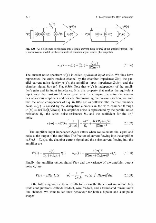
224 6 Electronics for Drift Chambers
en2(f)
in2(f)wi(f)Z(s) Z(s)=Zin(s)
gH(s) gH(s)
I(s) w(f)I(s) Zin(s)
Fig. 6.36 All noise sources collected into a single current noise source at the amplifier input. Thisis our universal model for the ensemble of chamber signal source plus amplifier
w( f ) = wi( f )+ i2n( f )+e2
n( f )|Z(iω)|2 . (6.106)
The current noise spectrum w( f ) is called equivalent input noise. We thus haverepresented the entire readout channel by the chamber impedance Z(s), the par-allel current noise density w( f ), the amplifier input impedance Zin(s), and thechamber signal I(s) (cf. Fig. 6.36). Note that w( f ) is independent of the ampli-fier’s gain and its input impedance. It is this property that makes the equivalentinput noise the most useful index upon which to compare the noise characteris-tics of various amplifiers and devices. Summarizing the previous section, we notethat the noise components of Eq. (6.106) are as follows: The thermal chambernoise wi( f ) is caused by the dissipative elements in the wire chamber throughwi(ω) = 4kT Re[1/Z(iω)]. The amplifier noise is represented by the parallel noiseresistance Rp, the series noise resistance Rs, and the coefficient for the 1/ fnoise:
w(ω) = 4kT Re
[1
Z(iω)
]+
4kTRp
+4kT Rs +B/ω
|Z(iω)|2 . (6.107)
The amplifier input impedance Zin(s) enters when we calculate the signal andnoise at the output of the amplifier. The fraction of current flowing into the amplifieris Z/(Z +Zin), so the chamber current signal and the noise current flowing into theamplifier are
Iin(s) =Z(s)
Z(s)+Zin(s)I(s) win( f ) =
|Z(iω)|2|Z(iω)+Zin(iω)|2 w( f ). (6.108)
Finally, the amplifier output signal V (s) and the variance of the amplifier outputnoise σ2
v are
V (s) = gH(s)Iin(s) σ2v =
12π
∫ ∞
0win(ω)g2|H(iω)|2dω. (6.109)
In the following we use these results to discuss the three most important elec-trode configurations: cathode readout, wire readout, and a terminated transmissionline channel. We want to see their behaviour for both a bipolar and a unipolarshaper.
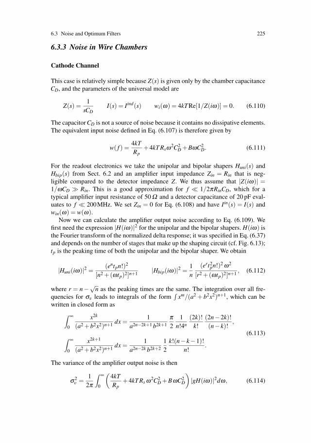
6.3 Noise and Optimum Filters 225
6.3.3 Noise in Wire Chambers
Cathode Channel
This case is relatively simple because Z(s) is given only by the chamber capacitanceCD, and the parameters of the universal model are
Z(s) =1
sCDI(s) = Iind(s) wi(ω) = 4kT Re[1/Z(iω)] = 0. (6.110)
The capacitor CD is not a source of noise because it contains no dissipative elements.The equivalent input noise defined in Eq. (6.107) is therefore given by
w( f ) =4kTRp
+4kT Rsω2C2D +BωC2
D. (6.111)
For the readout electronics we take the unipolar and bipolar shapers Huni(s) andHbip(s) from Sect. 6.2 and an amplifier input impedance Zin = Rin that is neg-ligible compared to the detector impedance Z. We thus assume that |Z(iω)| =1/ωCD � Rin. This is a good approximation for f 1/2πRinCD, which for atypical amplifier input resistance of 50 Ω and a detector capacitance of 20 pF eval-uates to f 200MHz. We set Zin = 0 for Eq. (6.108) and have Iin(s) = I(s) andwin(ω) = w(ω).
Now we can calculate the amplifier output noise according to Eq. (6.109). Wefirst need the expression |H(iω)|2 for the unipolar and the bipolar shapers. H(iω) isthe Fourier transform of the normalized delta response; it was specified in Eq. (6.37)and depends on the number of stages that make up the shaping circuit (cf. Fig. 6.13);tp is the peaking time of both the unipolar and the bipolar shaper. We obtain
|Huni(iω)|2 =(entpn!)2
[n2 +(ωtp)2]n+1 |Hbip(iω)|2 =1n
(ert2pn!)2 ω2
[r2 +(ωtp)2]n+1 , (6.112)
where r = n−√n as the peaking times are the same. The integration over all fre-
quencies for σv leads to integrals of the form∫
xm/(a2 + b2x2)n+1, which can bewritten in closed form as
∫ ∞
0
x2k
(a2 +b2x2)n+1 dx =1
a2n−2k+1 b2k+1
π2
1n!4n
(2k)!k!
(2n−2k)!(n− k)!
,
∫ ∞
0
x2k+1
(a2 +b2x2)n+1 dx =1
a2n−2k b2k+2
12
k!(n− k−1)!n!
.
(6.113)
The variance of the amplifier output noise is then
σ2v =
12π
∫ ∞
0
(4kTRp
+4kT Rs ω2C2D +BωC2
D
)|gH(iω)|2dω, (6.114)
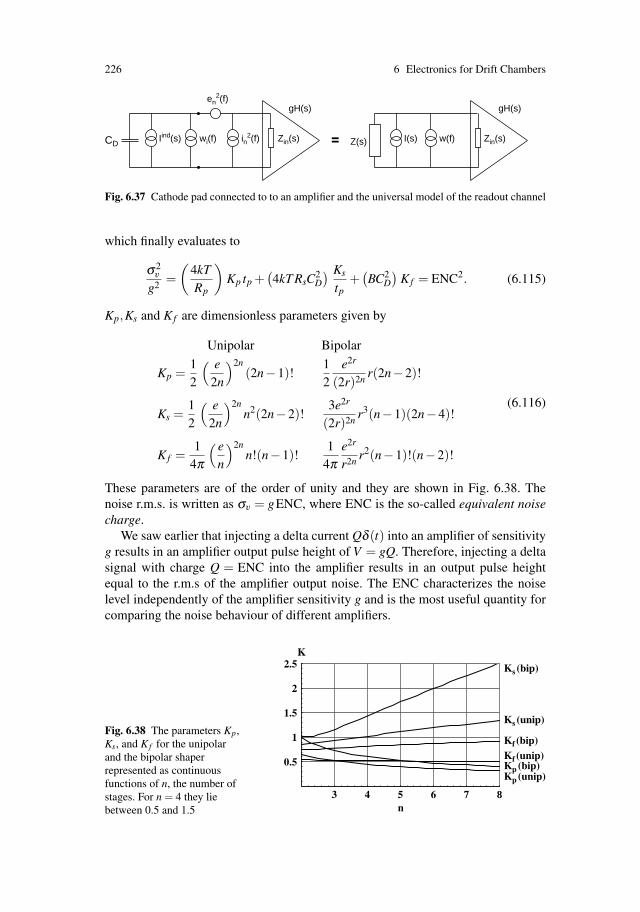
226 6 Electronics for Drift Chambers
en2(f)
in2(f)wi(f) Z(s)=Zin(s)
gH(s) gH(s)
Iind(s) w(f)I(s)CDZin(s)
Fig. 6.37 Cathode pad connected to to an amplifier and the universal model of the readout channel
which finally evaluates to
σ2v
g2 =(
4kTRp
)Kp tp +
(4kT RsC
2D
) Ks
tp+(BC2
D
)Kf = ENC2. (6.115)
Kp,Ks and Kf are dimensionless parameters given by
Unipolar Bipolar
Kp =12
( e2n
)2n(2n−1)!
12
e2r
(2r)2n r(2n−2)!
Ks =12
( e2n
)2nn2(2n−2)!
3e2r
(2r)2n r3(n−1)(2n−4)!
Kf =1
4π
( en
)2nn!(n−1)!
14π
e2r
r2n r2(n−1)!(n−2)!
(6.116)
These parameters are of the order of unity and they are shown in Fig. 6.38. Thenoise r.m.s. is written as σv = gENC, where ENC is the so-called equivalent noisecharge.
We saw earlier that injecting a delta current Qδ (t) into an amplifier of sensitivityg results in an amplifier output pulse height of V = gQ. Therefore, injecting a deltasignal with charge Q = ENC into the amplifier results in an output pulse heightequal to the r.m.s of the amplifier output noise. The ENC characterizes the noiselevel independently of the amplifier sensitivity g and is the most useful quantity forcomparing the noise behaviour of different amplifiers.
Fig. 6.38 The parameters Kp,Ks, and Kf for the unipolarand the bipolar shaperrepresented as continuousfunctions of n, the number ofstages. For n = 4 they liebetween 0.5 and 1.5
3 4 5 6 7 8n
0.5
1
1.5
2
2.5K
Ks (bip)
Kf (bip)
Kp (bip)
Ks (unip)
Kf (unip)
Kp (unip)

6.3 Noise and Optimum Filters 227
20 40 60 80 100
5001000150020002500300035004000
ENC (electrons)
20 40 60 80 100tp(ns)
5001000150020002500300035004000
ENC (electrons)
tp(ns)
S
1 2 1
S
2
3 3
(a) (b)
Fig. 6.39 Equivalent noise charge (ENC) as a function of the peaking time, calculated fromEq. (6.115). The three noise components are plotted separately, using typical values for the dif-ferent noise sources: parallel noise (Rp = 10kΩ ) curves 1, series noise (Rs = 150Ω ) curves 2, 1/ fnoise curves 3. The resulting total noise curves S exhibit a shallow minimum. (a) unipolar shaping,(b) bipolar shaping, both with n = 4
The three components of the ENC for the cathode channel are due to the parallelwhite noise, series white noise, and the 1/ f noise of the amplifier. The noise r.m.s.for the bipolar and the unipolar shaper as a function of amplifier peaking time isshown in Fig. 6.39. The three components of the noise exhibit a very distinct de-pendence on the amplifier peaking time. The parallel noise is proportional to
√tp,
whereas the series noise is proportional to 1/√
tp. The contribution from the 1/ fnoise is independent of the amplifier peaking time. The noise σv shows a minimumat the peaking time topt given by
topt = CD√
RsRp
√Ks
KpENC2
opt = 8kTCD
√Rs
Rp
√KsKp +BC2
DKf . (6.117)
The time constant τc = CD√
RsRp is the so-called noise corner time constant, sothe optimum peaking time is of the same order as τc. In the following we neglectthe small 1/ f component of the noise. For estimation of the order of magnitude fortopt and ENCopt we take an example where Rp = 10kΩ and Rs = 100Ω at roomtemperature T = 295 K, which results in
topt [ns] = CD[pF]
√Ks
KpENCopt = 350
√CD[pF](KsKp)1/4 electrons. (6.118)
Assuming a detector capacitance of Cd = 20–50 pF and that Kp and Ks are of theorder of unity, we find optimum peaking times in the range from 20–50 ns and ENCvalues between 1500 and 1800 electrons. We will see later that the minimum possi-ble ENC for any kind of shaping function is given by ENC2
min = 4kTCs√
Rs/Rp, sowe can rewrite the expression for the ENC as
ENC2(tp) = ENC2min
√4KpKs
12
(tp
topt+
topt
tp
). (6.119)
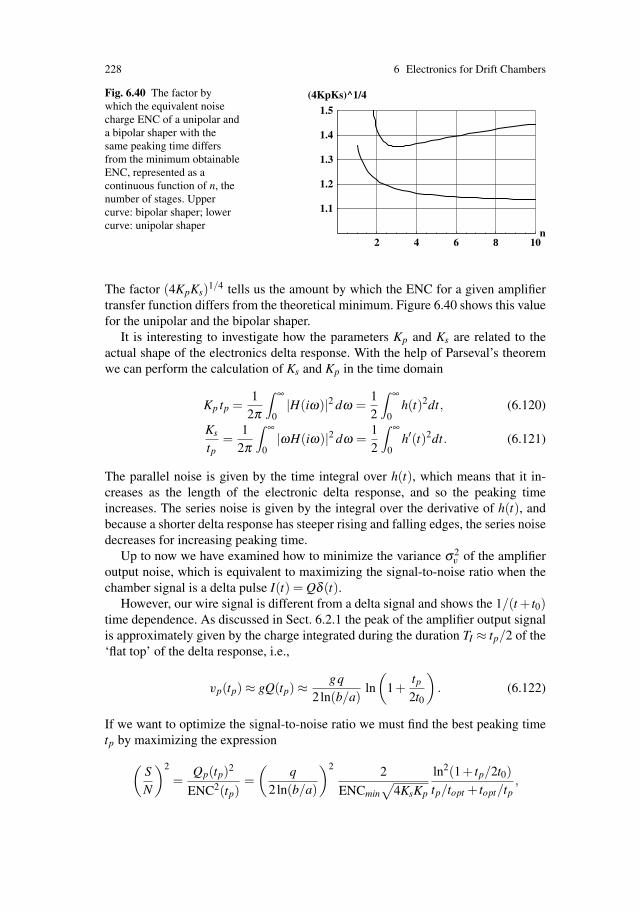
228 6 Electronics for Drift Chambers
Fig. 6.40 The factor bywhich the equivalent noisecharge ENC of a unipolar anda bipolar shaper with thesame peaking time differsfrom the minimum obtainableENC, represented as acontinuous function of n, thenumber of stages. Uppercurve: bipolar shaper; lowercurve: unipolar shaper
2 4 6 8 10n
1.1
1.2
1.3
1.4
1.5
(4KpKs)^1/4
The factor (4KpKs)1/4 tells us the amount by which the ENC for a given amplifiertransfer function differs from the theoretical minimum. Figure 6.40 shows this valuefor the unipolar and the bipolar shaper.
It is interesting to investigate how the parameters Kp and Ks are related to theactual shape of the electronics delta response. With the help of Parseval’s theoremwe can perform the calculation of Ks and Kp in the time domain
Kp tp =1
2π
∫ ∞
0|H(iω)|2 dω =
12
∫ ∞
0h(t)2dt, (6.120)
Ks
tp=
12π
∫ ∞
0|ωH(iω)|2 dω =
12
∫ ∞
0h′(t)2dt. (6.121)
The parallel noise is given by the time integral over h(t), which means that it in-creases as the length of the electronic delta response, and so the peaking timeincreases. The series noise is given by the integral over the derivative of h(t), andbecause a shorter delta response has steeper rising and falling edges, the series noisedecreases for increasing peaking time.
Up to now we have examined how to minimize the variance σ2v of the amplifier
output noise, which is equivalent to maximizing the signal-to-noise ratio when thechamber signal is a delta pulse I(t) = Qδ (t).
However, our wire signal is different from a delta signal and shows the 1/(t + t0)time dependence. As discussed in Sect. 6.2.1 the peak of the amplifier output signalis approximately given by the charge integrated during the duration TI ≈ tp/2 of the‘flat top’ of the delta response, i.e.,
vp(tp) ≈ gQ(tp) ≈gq
2ln(b/a)ln
(1+
tp
2t0
). (6.122)
If we want to optimize the signal-to-noise ratio we must find the best peaking timetp by maximizing the expression
(SN
)2
=Qp(tp)2
ENC2(tp)=(
q2ln(b/a)
)2 2
ENCmin√
4KsKp
ln2(1+ tp/2t0)tp/topt + topt/tp
,

6.3 Noise and Optimum Filters 229
Fig. 6.41 Optimum peakingtime tWire
opt for a wire chambersignal as a function of thetime constant t0, normalizedto tδ
opt which is the optimumpeaking time for a delta inputsignal
0.5 1 1.5 2
2.55
7.510
12.515
17.520
topt / topt
wire δ
t0 / toptδ
where topt gives the optimum signal-to-noise ratio for a delta input signal. The max-imum of the expression can only be found numerically, and Fig. 6.41 shows theoptimum peaking time as a function of the signal tail t0.
For t0 values that are much shorter than tδopt the wire chamber signal closely
resembles a delta pulse and the optimum peaking time for the wire readout is equaltδopt . In the case where t0 is similar to or longer than tδ
opt , the optimum peaking timetWireopt is longer because integrating more of the induced charge is still improving the
signal-to-noise ratio.
Terminated Transmission Line
If the signal propagation time along an electrode is of the same order as the signalpulse width as illustrated in Fig. 6.42, the electrode must be terminated in order toavoid multiple signal reflections. A transmission line with characteristic impedanceZ0 can be terminated with a resistor RT = Z0. In this case, Z(s) consists of a sim-ple resistor RT , which represents all the electrical characteristics of a terminatedtransmission line. The chamber model parameters are given by
Z(s) = RT I(s) = Iind(s) wi( f ) =4kTRT
. (6.123)
While the load resistor RL for the wire channel is usually dimensioned such thatit is a negligible source of noise compared to the amplifier noise, the termination
en2(f)
in2(f)wi(f) Zin(s)Z(s)=Zin(s)
gH(s) gH(s)
Iind(s) w(f)I(s)R
Fig. 6.42 Transmission line channel connected to to an amplifier and the universal model of thereadout channel

230 6 Electronics for Drift Chambers
resistor RT of a transmission line is uniquely defined by the chamber geom-etry and has typical values of 50–500 Ω . Therefore it is usually the termina-tion resistor noise that dominates over the amplifier noise for a transmission linereadout.
The equivalent input noise is
w( f ) =4kTRT
+ i2n +e2
n
R2T
=4kTRT
(1+
RT
Rp+
Rs
RT
)+
B
ωR2T
. (6.124)
For this discussion we neglect the 1/ f noise by setting B = 0, but because the orderof magnitude of the input impedance is similar to the chamber impedance we cannotneglect Zin as was done for the cathode channel. We therefore have
Iin(s) =RT
RT +RinI(s) = γ I(s) win( f ) = γ2 w( f ). (6.125)
The output noise for the unipolar and the bipolar shaper is therefore
σ2v = γ2g2 1
2π
∫ ∞
0win( f ) = g2γ2 4kT
RT
(1+
RT
Rp+
Rs
RT
)Kp tp. (6.126)
First we see that the noise r.m.s. is monotonically increasing with the peaking timetp, so the smallest noise r.m.s. is achieved for the shortest peaking time. To find theENC we send, as before, a delta signal Qδ (t) into the amplifier, which gives theoutput pulse height vp = gγQ, so the equivalent noise charge is
ENC2 =4kTRT
(1+
RT
Rp+
Rs
RT
)Kp tp = c1 tp. (6.127)
For the cathode channel discussed in the previous section, the noise is entirely de-fined by the amplifier noise i2n and e2
n and therefore depends only on the amplifierdesign. For the terminated transmission line channel, the noise of the terminationresistor represents an irreducible noise floor and the amplifier noise is negligiblewhen Rp � RT and Rs RT .
As before, we are interested in optimizing the signal-to-noise ratio for the wirechamber signal:
(SN
)2
=Qp(tp)2
ENC2(tp)=
(Q
2ln ba
)2ln2(1+ tp/2t0)
c1tp→ max .
The numerical evaluation shows that the expression has a maximum at tp ≈ 8 t0.If the input signal were a delta current pulse the signal-to-noise ratio would con-tinuously improve by reducing the amplifier peaking time. Since the wire chambersignal has a tail and the induced charge only increases with the logarithm of time,there is an optimum amplifier peaking time, that maximizes the signal-to-noiseratio.

6.3 Noise and Optimum Filters 231
en2(f)
in2(f)wi(f) Zin(s)Z(s)=Zin(s)
gH(s) gH(s)
Iind(s) w(f)I(s)RL
C
CD
Fig. 6.43 Wire connected to to an amplifier and the universal model of the readout channel
Wire Channel
The case shown in Fig. 6.43 contains more elements than there were for the cathodeand the transmission line channels. For the wire channel we have the followingelectrical parameters:
Z(s) =1
sC+
RL
1+ sRLCDI(s) =
sRLC1+ sRL(C +CD)
Iind(s)
wi( f ) =4kTRL
(ωRLC)2
1+(ωRL(C +CD))2 ≈ 4kTRL
for C �CD f � 12πRLC
.
The loading resistor RL is a source of thermal noise which is ‘filtered’ by the detectorcapacitance CD and the decoupling capacitor C. The expression for wi( f ) representsthe white noise of the resistor filtered by a high-pass filter with time constant τ =RLC. With the typical numbers of RL = 1 MΩ and C = 1 nF we have τ = 1ms.Therefore, only frequencies of f < 160 Hz are attenuated, which is negligible for thetypical amplifier bandwidth of a few MHz, and we can neglect the effect of C andCD. We assume again that the amplifier input resistance is negligible with respectto the chamber impedance and we also neglect the 1/ f noise term. The equivalentinput noise is then
w( f ) =4kTRL
+ i2n +ω2C2D e2
n +e2
n
R2L
=4kTRL
(1+
Rs
RL+
RL
Rp
)+4kT Rsω2C2
D. (6.128)
This expression has the same form as the one for the cathode channel and the resultsfrom there apply to this case as well.
We have seen that the unipolar shaper gives a better signal-to-noise ratio than thebipolar shaper, but the question arises as to whether one can improve the situationstill more by yet another kind of electronics transfer function. This problem can besolved in a remarkably general and elegant way, and it is possible find the maximumobtainable signal-to-noise ratio from the amplifier input signal and the spectral noisedensity at the amplifier input.
6.3.4 A Universal Limit on the Signal-to-Noise Ratio
In the last sections we found that we get different ENC values for different ampli-fier transfer functions, and that for a specific shape of a delta response there is an
232 6 Electronics for Drift Chambers
optimum peaking time. We found that the unipolar shaper results in a smaller ENCthan the bipolar shaper, and the question arises as to whether we can decrease thenoise level by yet another transfer function. Or going even further we can ask, whatis the maximum obtainable signal-to-noise ratio?
The reason the signal-to-noise ratio can be improved by specific filters is the factthe signal and the noise have different frequency spectra. So it is possible to improvethe signal-to-noise ratio by specific filters. The mathematical problem that we haveto solve can be formulated as shown in what follows.
A signal F(iω) with a superimposed noise having a power spectrum w(ω) isprocessed by an amplifier with transfer function H(iω). Which transfer functionH(iω) maximizes the signal-to-noise ratio?
Using Eq. 6.3 and 6.84 we can write the amplifier output signal g(t) and thevariance of the noise at the amplifier output as
g(t) =1
2π
∫ ∞
−∞F(iω)H(iω)eiωt dω σ2 =
12π
∫ ∞
0w(ω)|H(iω)|2 dω. (6.129)
The output signal g(t) has a maximum at some time tm when the signal-to-noiseratio S/N at the amplifier output is
(SN
)2
=(
g(tm)σ
)2
=1π
∣∣∫ ∞−∞ F(iω)H(iω)eiωtm dω
∣∣2∫ ∞−∞ w(ω)|H(iω)|2 dω
. (6.130)
This expression has an upper limit given by the Schwarz inequality, which gives thefollowing relation for two complex-valued functions ψ(x) and φ(x):
∣∣∣∣∫ b
aψ∗(x)φ(x)dx
∣∣∣∣2
≤∫ b
a|ψ(x)|2dx
∫ b
a|φ(x)|2dx, (6.131)
where the equal sign applies if ψ(x) = c1 φ(x) (c1 =const). If we insert
ψ(ω) =F∗(iω)√
w(ω)e−iωtm φ(ω) =
√w(ω)H(iω) (6.132)
and extend the integration limits to infinity, the inequality reads as
∣∣∣∣∫ ∞
−∞F(iω)H(iω)eiωtm dω
∣∣∣∣2
≤∫ ∞
−∞
|F(iω)|2w(ω)
dω∫ ∞
−∞w(ω)|H(iω)|2 dω, (6.133)
and therefore(
SN
)2
≤ 1π
∫ ∞
−∞
|F(iω)|2w(ω)
dω =2π
∫ ∞
0
|F(iω)|2w(ω)
dω . (6.134)
This result is remarkable in two respects. On the one hand, the solution to the prob-lem is surprisingly simple, while, on the other hand, the result has far-reachingconsequences: Whichever transfer function H(iω) we choose, the (S/N) will always

6.3 Noise and Optimum Filters 233
be lower than the value indicated above, which can be calculated in a straightforwardfashion from the signal and the noise spectrum at the amplifier input.
Now we would like to know the optimum transfer function H(iω) and the outputsignal G(iω). From the above relations we find that the equal sign applies if
F∗(iω)√w(ω)
e−iωtm = c1
√w(ω)H(iω) → H(iω) =
1c1
F∗(iω)w(ω)
e−iωtm . (6.135)
We can omit the factor exp(−iωtm) because it corresponds simply to a time delaytm according to Eq. (6.4e). This transfer function is unique up to a constant, andit provides the maximum signal-to-noise ratio. The amplifier output signal is thenproportional to
G(iω) = F(iω)H(iω) =|F(iω)|2
w(ω)g(t) = F−1[G(iω)]. (6.136)
We note that this signal g(t) is symmetric around t = 0 because G(iω) is real.As an example we consider a wire chamber cathode pad channel, where we found
a noise power spectrum of w(ω) = 4kT/Rp + 4kT RsC2Dω2 = a2 + b2ω2. Assum-
ing that the detector signal is a delta current pulse, we find the following optimumsignal-to-noise ratio
f (t) = Qδ (t) F(iω) = Q
(SN
)2
≤ 2π
∫ ∞
0
Q2
a2 +b2ω2 dω =Q2
ab(6.137)
The optimum transfer function is
H(iω) =1c1
Qa2 +b2ω2 h(t) = F−1[H(iω)] = c2e−|t|/τc τc =
ba. (6.138)
The time constant τc is called the noise corner time constant. The delta response ofthe optimum filter h(t) has a peak at t = 0 and is symmetric around t = 0 from whereit decays exponentially. This delta response is called the ‘infinite cusp’ function. Aswe saw earlier, a unipolar shaper with n = 6 results in a signal-to-noise ratio that isjust 15% worse than the optimum one that would be achieved by using the infinitecusp delta response.
The current signals in a wire chamber are not delta currents but have the hy-perbolic 1/(t + t0) form. If we use several pole-zero filters to remove the signaltail such that only a single exponential is left, the chamber signal is given byf (t) = A1 exp(−t/τ1) and the maximum achievable signal-to-noise ratio is smallerthan the one described above. By writing the signal amplitude in terms of the signalcharge Q =
∫f (t)dt = A1τ1, we have
f (t) =Qτ1
e−t/τ1 F(iω) =Qτ1
1iω +1/τ1
(SN
)2
≤ Q2
ab(1+ τ1/τc).
(6.139)

234 6 Electronics for Drift Chambers
In a previous section we found that it is very useful to approximate the cham-ber signal by a sum of exponentials, which can be done for every possible signalshape to any desired accuracy. By evaluating the above expressions for an in-put signal of the form f (t) = ∑N
n=1 An exp(−t/τn) we can find the maximumachievable signal-to-noise ratio for an arbitrary signal shape. We again write theamplitudes in terms of the charge ‘contained’ in each exponential Qn = Anτn. Theresult is
(SN
)2
≤ 1ab
N
∑n=1
N
∑m=1
Qm
1+ τm/τc
Qn
1+ τn/τc
[1+
2τmτn
τc(τn + τm)
]. (6.140)
The expression can be used to investigate by what factor the noise for a realisticamplifier transfer function deviates from the theoretical minimum.
6.4 Electronics for Charge Measurement
In the previous sections we discussed the processing of a wire chamber signal forseveral typical electrode configurations, including the effects of electronic noise. Upto now the signal induced on the electrode was assumed to have the form 1/(t + t0),which is characteristic for any electrode configuration as long as the avalanche elec-trons are moving in the coaxial region of the wire.
However, the signal shape applies only for a single electron that arrives at thewire and creates a single avalanche. It would also apply for a localized cloud ofelectrons arriving within a time shorter than t0. But the time spread of the incomingelectrons is generally much larger than t0, so the total signal is a superposition ofsingle-electron signals i0(t) = I0/(1+ t/t0),
iind(t) =N
∑n=1
Gni0(t − tn), (6.141)
with arrival times tn and avalanche sizes Gn. The output of the front-end electronicsis then also a linear superposition of the responses to the single electron pulses. Thequestion arises as to how we choose the transfer function H(iω) in order to arriveat the best signal-to-noise ratio for this situation. Clearly, the electron arrival timesvary from event to event and the electronics can only be adjusted for an averagesituation.
We first investigate the case of a TPC, where the arrival of the electrons at thesense wires assumes a Gaussian form owing to the diffusion along the drift path. Ifwe define an arrival time distribution n(t) such that n(t)dt is the average number ofelectrons that arrive between t and t +dt, we have
n(t)dt =N√2πσt
e−(t−T )2/2σ2t dt, (6.142)
6.5 Electronics for Time Measurement 235
where σt characterizes the electron diffusion along the drift path. Each arriving elec-tron will induce a signal of the form Gi0(t), where G is the gas gain, and the discretesum of time-delayed signals of Eq. (6.141) becomes a convolution of n(t) with i0(t):
i(t) = G∫ ∞
−∞i0(t − t ′)n(t ′)dt ′. (6.143)
We realize that from a formal point of view, the arrival time distribution n(t) en-ters like a linear signal processing device in an electronics chain. Using the Fouriertransform of n(t) we see that this becomes even more evident because we have
I(iω) = GI0(iω)N(iω). (6.144)
We can therefore apply all the results from the previous sections for optimizing theelectronic transfer function in order to achieve the best signal-to-noise ratio.
The optimum achievable signal-to-noise ratio for the average signal is given by
(SN
)2
=G2
π
∫ ∞
−∞
|I0(iω)N(iω)|2w(ω)
dω. (6.145)
If we assume that for reasons of high rate we remove the signal tail with a seriesof pole-zero filters such that the single electron signal assumes an exponential formwith a time constant τ which is negligible with respect to the arrival time distribu-tion, we can assume I0(t) = Qδ (t). If we assume in addition that the superimposednoise is white, the optimum transfer function according to Eq. (6.135) is
H(iω) =N∗(iω)
w0, (6.146)
a Gaussian with the same width as the arrival time distribution.With a wire chamber geometry shown in Chap. 7 the arrival time distribution will
be different from track to track, depending on the incident angle, the path lengthvariation, and diffusion. The distribution n(t) is given by the function fz(t,y) inEq. (7.7) and results in a width given by Eqs. (7.8) and (7.9). The optimizing processcan then be conducted as before. In general the optimum amplifier peaking time issuch that the width of the delta response is approximately equal to the electronarrival time distribution.
The actual measurement of the charge can be done in different ways. One eitherrecords the peak of the signal by a so-called ‘peak sensing ADC’, or one samplesthe signal at regular intervals and reconstructs the signal peak by fitting the knownresponse to the sample points.
6.5 Electronics for Time Measurement
In this section we investigate which front-end electronics should be used in orderto extract the best time information from the chamber signal. In drift chambers, thetime information is used to determine the track position by measuring the arrival
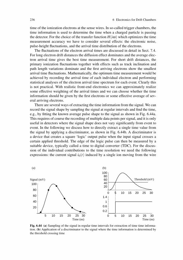
236 6 Electronics for Drift Chambers
time of the ionization electrons at the sense wires. In so-called trigger chambers, thetime information is used to determine the time when a charged particle is passingthe detector. For the choice of the transfer function H(iω) which optimizes the timemeasurement accuracy we have to consider several effects: the electronic noise,pulse-height fluctuations, and the arrival time distribution of the electrons.
The fluctuations of the electron arrival times are discussed in detail in Sect. 7.4.For long electron drift distances the diffusion effect dominates and the average elec-tron arrival time gives the best time measurement. For short drift distances, theprimary ionization fluctuations together with effects such as track inclination andpath length variations dominate and the first arriving electrons show the smallestarrival time fluctuations. Mathematically, the optimum time measurement would beachieved by recording the arrival time of each individual electron and performingstatistical analyses of the electron arrival time spectrum for each event. Clearly thisis not practical. With realistic front-end electronics we can approximately realizesome effective weighting of the arrival times and we can choose whether the timeinformation should be given by the first electrons or some effective average of sev-eral arriving electrons.
There are several ways of extracting the time information from the signal. We canrecord the signal shape by sampling the signal at regular intervals and find the time,e.g., by fitting the known average pulse shape to the signal as shown in Fig. 6.44a.This requires of course the recording of multiple data points per signal, and it is onlyuseful in detectors where the signal shape does not vary significantly from event toevent. In the following we discuss how to directly extract a single time value fromthe signal by applying a discriminator, as shown in Fig. 6.44b. A discriminator isa device that creates a square ‘logic’ output pulse when the input signal crosses acertain applied threshold. The edge of the logic pulse can then be measured by asuitable device, typically called a time to digital converter (TDC). For the discus-sion of the individual contributions to the time resolution we need the followingexpressions: the current signal i0(t) induced by a single ion moving from the wire
5 10 15 20 25 30
20406080
100
5 10 15 20 25 30
0.2
0.6
1.4
1
Time (ns)
0
0
Threshold (mV)
5 10 15 20 25 30
20
40
60
80
100
Signal (mV)
Time (ns)
(a) (b)
Fig. 6.44 (a) Sampling of the signal in regular time intervals for extraction of time time informa-tion. (b) Application of a discriminator to the signal where the time information is determined bythe threshold crossing time

6.5 Electronics for Time Measurement 237
surface towards the cathode and the amplifier output signal v0(t) for such an inputpulse:
i0(t) =I0
1+ t/t0v0(t) = g
∫ t
0h(t − t ′)i0(t ′)dt ′. (6.147)
From Fig. 6.16 and Eq. (6.44) we know that the peak v0p and the peak time Tp ofv0(t) are approximately given by
v0p ≈ gI0t0 ln(1+ tp/2t0) Tp ≈ tp (6.148)
for both the unipolar and the bipolar shaper.
6.5.1 Influence of Electronics Noise on Time Resolution
In order to isolate the effect of electronic noise from chamber intrinsic fluctuationswe first assume that m electrons arrive at the wire at exactly the same time and thatall electrons experience the same avalanche multiplication G. The induced current,the output signal and the peak of the output signal are then
i(t) = mGi0(t) v(t) = mGv0(t) vp ≈ gmGI0t0 ln(1+ tp/2t0) (6.149)
Applying a discriminator with a threshold vT to the amplifier output signal resultsin a measured time tT which, in the absence of electronic noise, is strictly related tothe arrival time of the electrons (Fig. 6.45). If electronic noise with an r.m.s of σv
is superimposed on the output signal v(t), the edge time of the discriminator outputwill vary, as illustrated in Fig. 6.46a. From the figure it is evident that the r.m.s. ofthe discriminator output time jitter is
σt =σv
k=
gENCk
k = v′(tT ), (6.150)
where k is the slope of v(t) at the threshold level. The slope k is proportional tovp/Tp, so we have
Fig. 6.45 Definition of theslope k at the thresholdcrossing, the signal peak timeTp, and the signal peak vp
5 10 15 20
0.2
0.4
0.6
0.8
1
0
Threshold
vp
vT
tT Tp
Slope k
Time (ns)
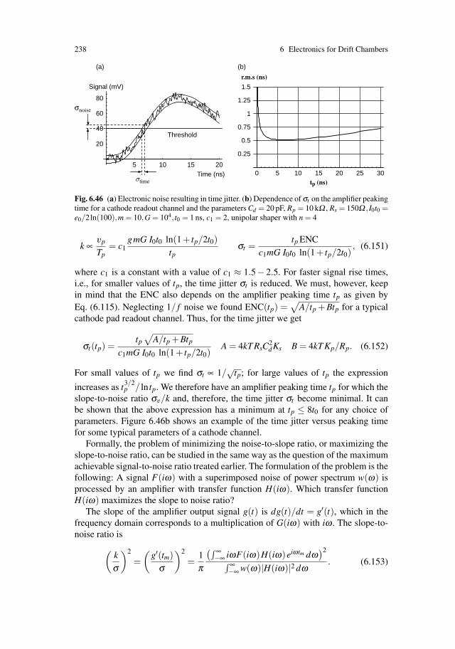
238 6 Electronics for Drift Chambers
5 10 15 20Time (ns)
20
40
60
(a) (b)
80
Signal (mV)
Threshold
σnoise
σtime5 10 15 20 25 30
0.25
0.5
0.75
1
1.5
0tp (ns)
r.m.s (ns)
1.25
Fig. 6.46 (a) Electronic noise resulting in time jitter. (b) Dependence of σt on the amplifier peakingtime for a cathode readout channel and the parameters Cd = 20 pF, Rp = 10 kΩ , Rs = 150Ω , I0t0 =e0/2ln(100),m = 10,G = 104, t0 = 1 ns, c1 = 2, unipolar shaper with n = 4
k ∝vp
Tp= c1
gmG I0t0 ln(1+ tp/2t0)tp
σt =tp ENC
c1mG I0t0 ln(1+ tp/2t0), (6.151)
where c1 is a constant with a value of c1 ≈ 1.5− 2.5. For faster signal rise times,i.e., for smaller values of tp, the time jitter σt is reduced. We must, however, keepin mind that the ENC also depends on the amplifier peaking time tp as given byEq. (6.115). Neglecting 1/ f noise we found ENC(tp) =
√A/tp +Btp for a typical
cathode pad readout channel. Thus, for the time jitter we get
σt(tp) =tp√
A/tp +Btp
c1mG I0t0 ln(1+ tp/2t0)A = 4kT RsC
2dKs B = 4kT Kp/Rp. (6.152)
For small values of tp we find σt ∝ 1/√
tp; for large values of tp the expression
increases as t3/2p / ln tp. We therefore have an amplifier peaking time tp for which the
slope-to-noise ratio σv/k and, therefore, the time jitter σt become minimal. It canbe shown that the above expression has a minimum at tp ≤ 8t0 for any choice ofparameters. Figure 6.46b shows an example of the time jitter versus peaking timefor some typical parameters of a cathode channel.
Formally, the problem of minimizing the noise-to-slope ratio, or maximizing theslope-to-noise ratio, can be studied in the same way as the question of the maximumachievable signal-to-noise ratio treated earlier. The formulation of the problem is thefollowing: A signal F(iω) with a superimposed noise of power spectrum w(ω) isprocessed by an amplifier with transfer function H(iω). Which transfer functionH(iω) maximizes the slope to noise ratio?
The slope of the amplifier output signal g(t) is dg(t)/dt = g′(t), which in thefrequency domain corresponds to a multiplication of G(iω) with iω . The slope-to-noise ratio is
(kσ
)2
=(
g′(tm)σ
)2
=1π
(∫ ∞−∞ iωF(iω)H(iω)eiωtm dω
)2
∫ ∞−∞ w(ω)|H(iω)|2 dω
. (6.153)

6.5 Electronics for Time Measurement 239
Proceeding as before we find the maximum achievable slope-to-noise ratio
(kσ
)2
≤ 2π
∫ ∞
0
|ωF(iω)|2w(ω)
dω (6.154)
with the optimum transfer function H(iω) and the output signal G(iω) being
H(iω) = iωF∗(iω)w(ω)
e−iωtm G(iω) = iω|F(iω)|2
w(ω)e−itmω . (6.155)
We realize that H(iω) and G(iω) differ only by the factor iω from the filters op-timizing the signal-to-noise ratio that we found earlier. Since a multiplication withiω in the frequency domain corresponds to the derivative in the time domain we canconclude:
For a given signal f (t) and noise power spectrum w(ω), the amplifier deltaresponse that maximizes the slope-to-noise ratio is equal to the derivative of theamplifier delta response that maximizes the signal-to-noise ratio.
Since the amplifier output signal for maximizing the signal-to-noise ratio is sym-metric around t = 0, the amplifier output signal optimizing the slope-to-noise ratiois antisymmetric around zero and the maximum slope-to-noise ratio is found at thezero crossing timer of the signal (Fig. 6.47).
6.5.2 Influence of Pulse-Height Fluctuations on Time Resolution
We now consider the same situation as before, where m electrons arrive at the sametime at the sense wire, but we let the number m fluctuate from event to event accord-ing to a distribution p(m) with an average of m and an r.m.s. of σm (Fig. 6.48a).Although all the electrons arrive at the same time, we find different threshold
5 10 15 20 25
1
0.5
0
0.5
1
Time (ns)
Fig. 6.47 Example for the output signal of two optimum filters. The symmetric curve is the outputsignal for a filter that maximizes the signal-to-noise ratio. The antisymmetric curve is the output ofa filter that maximizes the slope-to-noise ratio. The maximum slope-to-noise ratio is found at thezero crossing. The delta response of the filter that maximizes the slope-to-noise ratio is equal tothe time derivative of the delta response for the filter that maximizes the signal-to-noise ratio. Thesame is true for the output signals of the two filters

240 6 Electronics for Drift Chambers
Time (ns)
Threshold
(a)
5 10 15 20 25
–1
–0.5
0.5
1
0Time (ns)
(b)
5 10 15 20
0.2
0.4
0.6
0.8
1
Fig. 6.48 (a) Variations of the pulse height result in different threshold crossing times. The effectis called ‘time walk’. (b) The zero crossing time of a bipolar pulse is independent of the pulseheight
crossing times owing to the pulse-height variations of the signal, an effect that iscalled ‘time walk’. The threshold crossing time and its variance are
tT (m) =vT
k(m)σt ≈ σm
dtT (m)dm
|m=m =tp vT
c1mGI0t0 ln(1+ tp/2t0)
(σm
m
).
(6.156)We see that the time walk decreases linearly with the threshold and the peakingtime and we therefore want fast electronics and the lowest possible threshold forachieving the best time resolution. However, the lowest possible threshold is againdetermined by the noise. The frequency fT of the noise threshold crossings for athreshold vT is given by
fT = fzero e−v2T /2σ2
v , (6.157)
where fzero is the number of zero crossings from Eq. (6.83) [RIC 44]. Setting thethreshold vT to 1,2,3,4,5 times the noise r.m.s. results in a threshold crossing fre-quency of 0.6,0.14,0.01,3.3×10−4,3.7×10−6 times fzero. With fzero being in therange of 10–100 MHz we have to set the threshold vT to at least five times the noiser.m.s. in order to arrive at a noise count rate of less than 100 Hz. We use vT = 5σv
in the following. The discriminator threshold vT is typically expressed as a chargeaccording to vT = gQT in order to arrive at expressions independent of the ampli-fier sensitivity. The amplifier output noise is σv = gENC, and we therefore have athreshold of QT = 5ENC:
σt =tp 5√
A/tp +Btp
c1mGI0t0 ln(1+ tp/2t0)
(σm
m
). (6.158)
This expression is equal to the expression for the time jitter up to a factor 5σm/m.Therefore the peaking time that minimizes the jitter due to electronic noise alsominimizes the jitter due to pulse-height variations. The combined effect of electronicnoise and pulse-height fluctuations becomes
σt =√
σ2jitter +σ2
walk =
√1+(
5σm
m
)2 tp√
A/tp +Btp
c1mGI0t0 ln(1+ tp/2t0). (6.159)
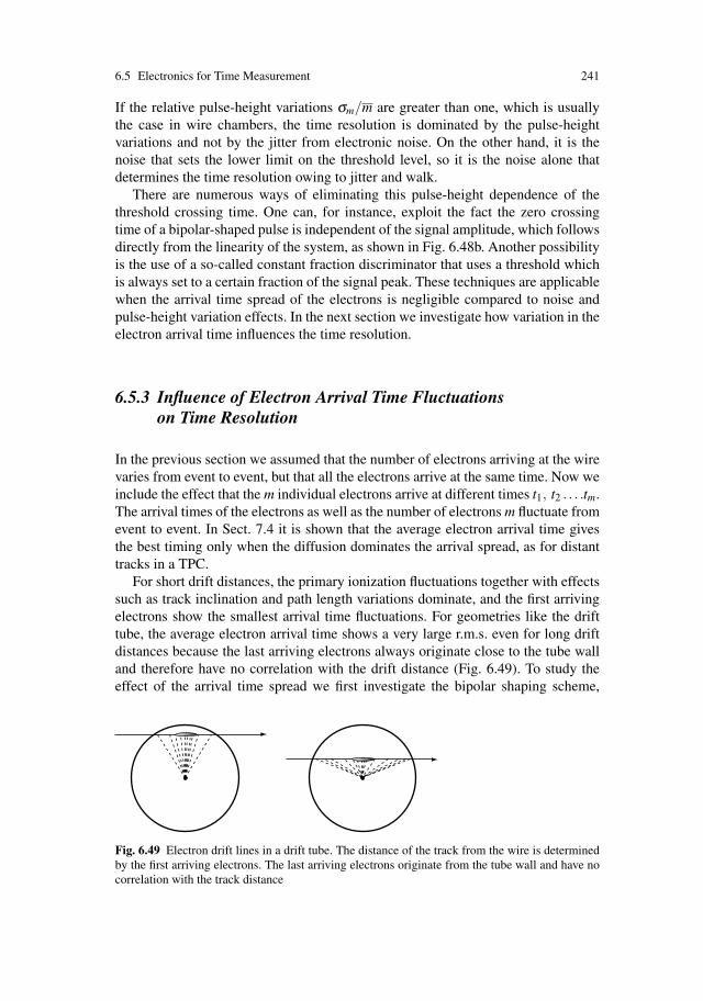
6.5 Electronics for Time Measurement 241
If the relative pulse-height variations σm/m are greater than one, which is usuallythe case in wire chambers, the time resolution is dominated by the pulse-heightvariations and not by the jitter from electronic noise. On the other hand, it is thenoise that sets the lower limit on the threshold level, so it is the noise alone thatdetermines the time resolution owing to jitter and walk.
There are numerous ways of eliminating this pulse-height dependence of thethreshold crossing time. One can, for instance, exploit the fact the zero crossingtime of a bipolar-shaped pulse is independent of the signal amplitude, which followsdirectly from the linearity of the system, as shown in Fig. 6.48b. Another possibilityis the use of a so-called constant fraction discriminator that uses a threshold whichis always set to a certain fraction of the signal peak. These techniques are applicablewhen the arrival time spread of the electrons is negligible compared to noise andpulse-height variation effects. In the next section we investigate how variation in theelectron arrival time influences the time resolution.
6.5.3 Influence of Electron Arrival Time Fluctuationson Time Resolution
In the previous section we assumed that the number of electrons arriving at the wirevaries from event to event, but that all the electrons arrive at the same time. Now weinclude the effect that the m individual electrons arrive at different times t1, t2 . . . .tm.The arrival times of the electrons as well as the number of electrons m fluctuate fromevent to event. In Sect. 7.4 it is shown that the average electron arrival time givesthe best timing only when the diffusion dominates the arrival spread, as for distanttracks in a TPC.
For short drift distances, the primary ionization fluctuations together with effectssuch as track inclination and path length variations dominate, and the first arrivingelectrons show the smallest arrival time fluctuations. For geometries like the drifttube, the average electron arrival time shows a very large r.m.s. even for long driftdistances because the last arriving electrons always originate close to the tube walland therefore have no correlation with the drift distance (Fig. 6.49). To study theeffect of the arrival time spread we first investigate the bipolar shaping scheme,
Fig. 6.49 Electron drift lines in a drift tube. The distance of the track from the wire is determinedby the first arriving electrons. The last arriving electrons originate from the tube wall and have nocorrelation with the track distance

242 6 Electronics for Drift Chambers
5 10 15 20
2
1
1
2
Time (ns)
15 20 25 30
0.5
1
1.5
2
2.5
3
12.5 13 13.5 14 14.5 15
0.3
0.4
0.5
9.5 10 10.5 11 11.5 12
0.4
0.2
0.2
0.4
0Time (ns)
Time (ns)
(a) (b)
(c) (d)
Time (ns)
Fig. 6.50 Pulses from three electrons arriving at the wire at different times. The solid lines showthe pulses of the individual electrons; the dotted lines correspond to the sum of the pulses giv-ing the measured chamber signal. Parts (a) and (b) show the bipolar-shaped signals where thetime measurement is given by the zero crossing of the chamber signal. Parts (c) and (d) showthe unipolar-shaped signals where the time measurement is given by the threshold crossing of thechamber signal. The two schemes have distinctly different timing properties
where the zero crossing of the signal determines the measurement time. Figure 6.50ashows the signals from three individual electrons arriving at different times and theresulting chamber signal which is the sum of the individual electron signals. Aroundthe zero crossing the electron signals can be approximated by a straight line with aslope −k (Fig. 6.50b), and the individual electron signals vi(t) and the resultingsignal v(t) can be approximated by
vi(t) = −k(t − ti) v(t) =m
∑i=1
vi(t) = −k mt − km
∑i=1
ti. (6.160)
The zero crossing time tT of the signal v(t) is
v(t) = 0 → tT =1m
m
∑i=1
ti = t (6.161)
and equal to the average arrival time of the m electrons. This scheme is thereforeapplicable for the ‘diffusion dominated’ cases mentioned above.
If we want the nth electron to give the timing information we can imagine anamplifier that produces a step function output signal of amplitude v0 for a single
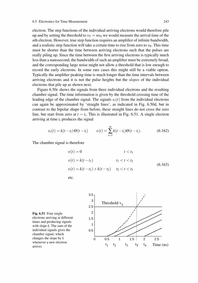
6.5 Electronics for Time Measurement 243
electron. The step functions of the individual arriving electrons would therefore pileup and by setting the threshold to vT = nv0 we would measure the arrival time of thenth electron. However, true step function requires an amplifier of infinite bandwidth,and a realistic step function will take a certain time to rise from zero to v0. This timemust be shorter than the time between arriving electrons such that the pulses arereally piling up. Since the time between the first arriving electrons is typically muchless than a nanosecond, the bandwidth of such an amplifier must be extremely broad,and the corresponding large noise might not allow a threshold that is low enough torecord the early electrons. In some rare cases this might still be a viable option.Typically the amplifier peaking time is much longer than the time intervals betweenarriving electrons and it is not the pulse heights but the slopes of the individualelectrons that pile up as shown next.
Figure 6.50c shows the signals from three individual electrons and the resultingchamber signal. The time information is given by the threshold crossing time of theleading edge of the chamber signal. The signals vi(t) from the individual electronscan again be approximated by ‘straight lines’, as indicated in Fig. 6.50d, but incontrast to the bipolar shape from before, these straight lines do not cross the zeroline, but start from zero at t = ti. This is illustrated in Fig. 6.51. A single electronarriving at time ti produces the signal
vi(t) = k(t − ti)Θ(t − ti) v(t) =m
∑i=1
k(t − ti)Θ(t − ti). (6.162)
The chamber signal is therefore
v(t) = 0 t < t1
v(t) = k(t − t1) t1 < t < t2
v(t) = k(t − t1)+ k(t − t2) t2 < t < t3
etc.
(6.163)
Fig. 6.51 Four singleelectrons arriving at differenttimes and producing signalswith slope k. The sum of theindividual signals gives thechamber signal, whichchanges the slope by kwhenever a new electronarrives
0.5 1 1.5 2 2.5
0.5
1
1.5
2
2.5
3
3.5
0
Time (ns)
Threshold vT
t1 t2 t3 tT t4

244 6 Electronics for Drift Chambers
and in general we get
v(t) =n
∑i=1
k(t − ti) = k nt − kn
∑i=1
ti tn < t < tn+1. (6.164)
Whenever a new electron arrives the slope changes by k, and after the arrival of thenth electron the signal slope is ks = nk. The threshold crossing time tT is
v(t) = vT → tT =1n
n
∑i=1
ti +vT
kn= t<n +
vT
knif tn < tT < tn+1. (6.165)
We see that the threshold crossing time is equal to the average arrival time of the nelectrons that arrived before the threshold crossing plus another term that is inverselyproportional to n. Figure 6.51 shows an example in which four electrons arrive attimes t1, t2, t3, and t4. The chamber signal crosses the threshold before the arrival ofthe fourth electron, so we have n = 3 and the threshold crossing time is
tT =13(t1 + t2 + t3)+
vT
3k. (6.166)
If all the electrons arrive at the same time t = 0 we are left with only the secondterm, which is equal to the expression for the time walk discussed in the previoussection. We can therefore state that the first term is due to the electron arrival timespread and the second term to the varying number of electrons that contribute to thesignal at the threshold crossing time. However, the two expressions correlate in acomplex way.
If we want to explicitly calculate the threshold crossing time distribution and itsr.m.s., it is not sufficient to know the average and r.m.s of the arrival distribution forthe nth electron. The threshold crossing time depends on the arrival times of all nelectrons, so we need the probability density
P(t1, t2, t3 . . .)dt1dt2dt3 . . . , (6.167)
which gives the probability that the first electron arrives in the time interval t1, t1 +dt1, the second arrives in the time interval t2, t2 +dt2, etc. The distribution P(t1, t2 . . .)is typically generated with a Monte Carlo simulation program. Instead of finding ananalytic parametrization of the Monte Carlo generated distributions and evaluatingthe integrals of the probability distribution it is much easier to record the arrivaltime pattern t1, . . .tm for each Monte Carlo event and to find the chamber signal bysuperimposing the single-electron pulse v0(t) according to
v(t) =m
∑i=1
v0(t − ti). (6.168)
By adding the expected noise signal to v(t) we find a set of pulses from whichwe can calculate the threshold crossing times and therefore the time r.m.s. This
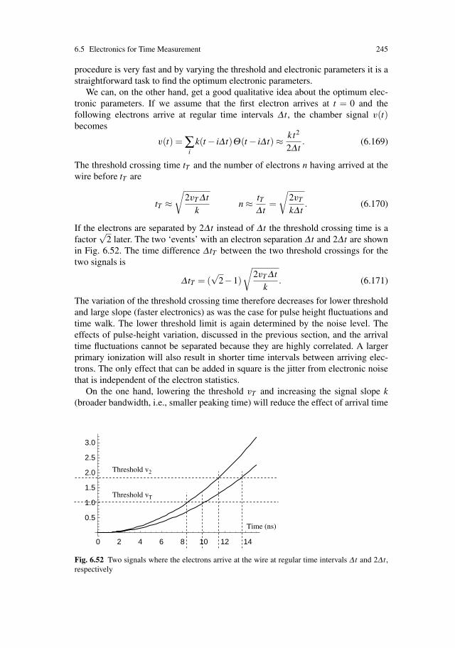
6.5 Electronics for Time Measurement 245
procedure is very fast and by varying the threshold and electronic parameters it is astraightforward task to find the optimum electronic parameters.
We can, on the other hand, get a good qualitative idea about the optimum elec-tronic parameters. If we assume that the first electron arrives at t = 0 and thefollowing electrons arrive at regular time intervals Δ t, the chamber signal v(t)becomes
v(t) = ∑i
k(t − iΔ t)Θ(t − iΔ t) ≈ kt2
2Δ t. (6.169)
The threshold crossing time tT and the number of electrons n having arrived at thewire before tT are
tT ≈√
2vT Δ tk
n ≈ tTΔ t
=
√2vT
kΔ t. (6.170)
If the electrons are separated by 2Δ t instead of Δ t the threshold crossing time is afactor
√2 later. The two ‘events’ with an electron separation Δ t and 2Δ t are shown
in Fig. 6.52. The time difference Δ tT between the two threshold crossings for thetwo signals is
Δ tT = (√
2−1)
√2vT Δ t
k. (6.171)
The variation of the threshold crossing time therefore decreases for lower thresholdand large slope (faster electronics) as was the case for pulse height fluctuations andtime walk. The lower threshold limit is again determined by the noise level. Theeffects of pulse-height variation, discussed in the previous section, and the arrivaltime fluctuations cannot be separated because they are highly correlated. A largerprimary ionization will also result in shorter time intervals between arriving elec-trons. The only effect that can be added in square is the jitter from electronic noisethat is independent of the electron statistics.
On the one hand, lowering the threshold vT and increasing the signal slope k(broader bandwidth, i.e., smaller peaking time) will reduce the effect of arrival time
2 4 6 8 10 12 14
0.5
1.0
1.5
2.0
2.5
3.0
0
Threshold vT
Threshold v2
Time (ns)
Fig. 6.52 Two signals where the electrons arrive at the wire at regular time intervals Δ t and 2Δ t,respectively

246 6 Electronics for Drift Chambers
fluctuations and related pulse-height fluctuations. On the other hand, a broader band-width will increase the noise and a lower threshold will increase the noise jitterbecause of the parabolic shape of the signal. The compromise between these twotendencies will define the optimum amplifier peaking time, which will again be ofthe order of a few times t0.
Finally we note that the slope of the signal at the threshold crossing time ks = nkmeasures the number of electrons that have contributed to the signal, and by usingthis information we can improve the time resolution. The slope can, for example,be measured by a second threshold (Fig. 6.52) or by a device that measures thesignal charge in a short time interval following the threshold crossing time. Thistechnique is known as amplitude and rise time compensation and allows extractionof the optimum time information from the signal.
6.6 Three Examples of Modern Drift Chamber Electronics
In this last section we present some front-end electronics examples that are beingused in large detector systems. We discuss an amplifier for time measurement used atrates up to 15 MHz, an amplifier for charge measurement in a cathode strip chamber,and a front-end system for a TPC.
6.6.1 The ASDBLR Front-end Electronics
The ASDBLR (amplifier shaper discriminator baseline restorer) chip [BEN 96] is aneight-channel front-end chip developed for readout of the ATLAS [ATL 94] transi-tion radiation tracker [AKE 04]. The chip is implemented in a radiation hard bipolarprocess. The tracker consists of almost half a million drift tubes of 4 mm diame-ter with a 30-μm-diameter anode wire. A xenon-based gas mixture at a gas gainof ≈ 2× 10⁴ is used. The goal is a spatial resolution of better than 150 μm at ex-treme rates of up to 15 MHz. To cope with this high rate, unipolar signal shapingwas chosen. The ASDBLR circuit is based on a front-end described in [FIS 85], andthe equivalent block diagram is equal to the one shown in Fig. 6.27 top. It consistsof a large bandwidth preamplifier with 1 ns rise time followed by a unipolar shaper(n = 3) that provides a peaking time of tp = 8ns. The preamp input impedance ofRin = 295Ω is matched to the characteristic impedance of the drift tube, which rep-resents a capacitance of CD ≈ 12pF. A double pole-zero network cancels the signaltail. In order to provide the baseline stability at the very high rates, the shaper isfollowed by a fast (nonlinear) baseline restoration circuit using diodes. For verysmall signals, the BLR acts like a CR differentiation circuit and produces a bipolaroutput. As the shaper signals grow in magnitude, the exponential behaviour of thediodes causes the undershoot to rise logarithmically with the pulse height, whichresults in a unipolar signal shape. With this signal processing chain, the return to

6.6 Three Examples of Modern Drift Chamber Electronics 247
baseline is 30 ns for a vp/g = 2-fC pulse and 60 ns for a vp/g = 200-fC pulse. Theachieved ENC with attached drift tube is approximately 2300 electrons. The sen-sitivity of g = 20 mV/fC provides a full-scale linear range for pulse heights from0 to vp/g = 200 fC. The last circuit element is a discriminator with two thresholdsproviding the leading edge time (low threshold) and the identification of an X-rayphoton hit (high threshold). A single-wire resolution of 100 μm and efficiency of80% at low rate is achieved. At a rate of 17 MHz, the resolution is 120 μm and theefficiency is 50% [AKE 04].
6.6.2 The ATLAS CSC Front-end Electronics
The ATLAS CSC fronted chip [OCO 99][JUN 05] is designed for readout of theATLAS cathode strip chambers [BEN 95]. These chambers measure muon trackswith an accuracy of ≈ 50 μm by using charge interpolation of cathode strips with apitch of 5.08 mm. The chambers are multiwire proportional chambers with a wirepitch and wire-to-cathode distance of 2.54 mm. The gas used is an Ar/CO2 mixtureoperated at a gas gain of 2× 10⁴. For a pitch of 5 mm and the specified positionresolution of 50 μm, a signal-to-noise ratio of about 150 is required. This leads to aspecification for an ENC of less than 2500 electrons for the chosen operating point.The cathode strip capacitance ranges from 50 to 100 pF.
The front-end electronics developed for this detector consists of a bipolar shaperwith a peaking time of 75 ns, resulting in a total pulse length of about 300 ns. Thisnumber is a compromise between noise performance and the inefficiency at thehighest expected rates of about 600 kHz. This bipolar shaper is not the one describedin the previous sections, but a shaper with one real pole and six complex poles,called a seventh- order complex Gaussian filter [OHK 76]. It has the advantage of amore symmetric response compared to the bipolar shaper realized by an equivalentnumber of real coincident poles and having the same pulse-width. The achievednoise performance is 1140+17.6 e−/pF. The sensitivity is 3.8 mV/fC, which allowsa linear range of 450 fC. A single chip of 3.29×5.79 mm size contains 25 channelsand the power dissipation amounts to 32.5 mW/channel. The output signals are thensampled at a 20 MHz rate and readout on a level 1 trigger to a 12 bit analog todigital converter (ADC).
6.6.3 The PASA and ALTRO Electronics for the ALICE TPC
The PASA (preamplifier shaper) chip together with ALTRO (alice TPC readout)chip [MUS 03] form the front-end of the time projection chamber for the ALICE[ALI 95] [APP 99] experiment. This ALICE TPC consists of a cylindrical gas vol-ume of about 90 m3 under a uniform electrostatic field and a drift distance of upto 2.5 m. At the endplates, multiwire proportional chambers provide a readout by

248 6 Electronics for Drift Chambers
means of a cathode plane segmented into about 6× 10⁵ pads. These pads are con-nected to the PASA chip, a 16-channel amplifier chip providing a delta responsewith a peaking time of tp ≈ 150 ns and a full width at half maximum of about 200 ns.The peaking time is realized by two so-called T-bridge second-order shapers result-ing in two pairs of real poles. The transfer function is, however, very similar to ann = 4 unipolar shaper. The diffusion of the gas used is quoted as 220 μm/
√cm, so a
diffusion of σ = 2.2 mm at a drift distance of 100 cm and σ = 3.5 mm at a drift dis-tance at 250 cm is expected. With a drift velocity of 28.3 μm/ns this corresponds toa FWHM of the arriving electron cloud of 180 and 290 ns. The choice of 200 ns forthe FWHM of the shaper is therefore a compromise in terms of optimum signal-to-noise ratio and pulse width. The ENC of the PASA chip is < 1000 electrons in orderto allow a signal-to-noise ratio of 30 at the specified working point. The sensitivityis g = 12 mV/fC with a linear range of 2 V.
The signal from the PASA is then fed into the ALTRO chip [BOS 03], whichintegrates 16 channels, each consisting of a 10-bit, 10 MS/s ADC, followed by aprogrammable digital baseline subtraction and tail cancellation filter, a zero suppres-sion unit, and a multi-event buffer. All this functionality is contained in an 8×8mmCMOS chip. The tail cancellation filter can be programmed to represent any fourth-order filter, i.e., any transfer function consisting of a fourth-order polynomial in thenumerator and the denominator. The advantage of such an approach is evident: Thesignal tail cancellation time constants do not have to be hardwired into the front-endelectronic chip but are fully programmable, which provides maximum flexibility.Clearly, the integration of the front-end chip in the ALTRO is a desirable next step.
We conclude this section by noting that the extreme miniaturization of micro-electronic components, together with the reduced power consumption, has allowedthe placement of a large number of electronic channels very close to the detector,which makes the systems very compact and economic.
References
[AKE 04] T. Akesson et al., Operation of the ATLAS Transition Radiation Tracker under veryhigh irradiation at the CERN LHC, Nucl. Instr. Meth. Phys. Res. A 552, 25–32 (2004)
[ALI 95] Technical proposal for a Large Ion Collider Experiment at the CERN LHC, CERN,Geneva, Switzerland, CERN/LHCC 95–71, 1995
[ATL 94] ATLAS Collaboration, Technical Proposal for a General Purpose pp Experiment at theLarge Hadron Collider at CERN, CERN, Geneva, Switzerland, CERN/LHCC/94–43,1994
[BEN 95] G. Bencze et al., Position and timing resolution of interpolating cathode strip chambersin a test beam, Nucl. Instr. Meth. Phys. Res. A 357, 40–54 (1995)
[BEN 96] B. Benvensee, F.M. Newcomer, R. Van Berg, and H.H. Williams, An amplifier-shaper-discriminator with baseline restoration for the ATLAS transition radiation tracker,IEEE Trans. Nucl. Sci. 43, 1725–1731 (1996)
[BOI 82] R.A. Boie, A.T. Hrisoho, P. Rehak, Signal shaping and tail cancellation for gas propor-tional detectors at high counting rates, Nucl. Instr. Meth. Phys. Res. A 192, 365–374(1982)
References 249
[BOS 03] R.E. Bosch, A.J. de Parga, B. Mota and L. Musa, The ALTRO Chip: a 16-channel A/Dconverter and digtal processor for gas detectors, IEEE Trans. Nucl. Sci. 50, 2460–2469(2003)
[FIS 85] J. Fischer, A. Hrisoho, V. Radeka, P. Rehak, Proportional chambers for very highcounting rates based on gas mixtures of CF4 with hydrocarbons, Nucl. Instr. Meth.Phys. Res. A 238, 249–264 (1985)
[GAT 85] E. Gatti and P.F. Manfredi, Processing the Signals from Solid-State Detectors inElementary-Particle Physics, RIV Nuovo Cimento 9(1), (1986)
[HOR 89] P. Horowitz and W. Hill, The Art of Electronics, 2nd edition, (Cambridge UniversityPress, 1989)
[JOH 28] J.B. Johnson, Thermal agitation of electricity in conductors, Phys. Rev. 32, 97–109(1928)
[JUN 05] S.S. Junnakar et al., Advanced front end signal processing electronics for ATLAScathode strip chamber system, IEEE Nucl. Sci. Symp. Conf. Rec. 2, 909–913 (2005)
[KIT 58] C. Kittel, Elementary Statistical Physics, (John Wiley & Sons, New York 1958)[MOT 93] C.D. Motchenbacher and J.A. Connelly, Low-Noise Electronic System Design, (John
Wiley & Sons, New York 1993)[MUS 03] L. Musa et al., The ALICE TPC front end electronics, IEEE Nucl. Sci. Symp. Conf.
Rec. 5, 3647–3651 (2003)[NAH 03] M. Nahvi and J. Edminister, Schaum’s Outline Series, Electric Circuits, 4th edition,
(McGraw-Hill, New York 2003)[NIC 73] P.W. Nicholson, Nuclear Electronics, (John Wiley & Sons, 1973)[NYQ 28] H. Nyquist, Thermal agitation of electric charge in conductors, Phys.Rev. 32, 110–114
(1928)[OCO 99] P. O’Connor et al., Readout electronics for a high-rate CSC detector, Proceedings of
the Fifth Workshop on Electronics for LHC Experiments, CERN, Geneva, Switzerland,452–456 (1999)
[OHK 76] S. Ohkawa, M. Yoshizawa, K. Husimi, Direct synthesis of the Gaussian filter for nu-clear pulse amplifiers, Nucl. Instr. Meth. 138, 85–92 (1976)
[OPP 97] A.V. Oppenheim and A.S. Willsky, S.H. Nawab, Signals and Systems, 2nd edition,(Prentice Hall International, 1997)
[RAD 88] V. Radeka, Low-Noise Techniques in Detectors, Ann. Rev. Nucl. Part. Sci. 38, 217–277(1988)
[REH 83] P. Rehak, Detection and Signal Processing In High-Energy Physics, LXXXIV CorsoSoc. Italiana di Fisica - Bologna - Italy, 1983
[RIC 44] S.O. Rice, Mathematical Analysis of Random Noise, Bell Syst. techn. J. 23, 282(1944), 24, 46 (1945), reprinted in: N. Wax, Selected Papers on Noise and StochasticProcesses, (Dover Publications, New York 1954, 2003)
[ROB 74] F.N.H. Robinson, Noise and fluctuations in electronic devices and circuits, Mono-graphs in Electrical and Electronics Engineering, (Clarendon Press, Oxford 1974)
[TPC 99] ALICE time projection chamber: Technical Design Report, CERN, Geneva, Switzer-land, CERN/LHCC 2000–001, 1999


Chapter 7Coordinate Measurement and FundamentalLimits of Accuracy
7.1 Methods of Coordinate Measurement
After the passage of a charged particle through the sensitive gas volume, the elec-trons produced in the ionization process along a trajectory segment drift toward thesense wire, where they are collected and amplified in avalanches. There are essen-tially four different methods to determine particle coordinates in drift chambers:
1. Measurement of the drift time. Using the known drift velocity of the ionizationelectrons along their drift trajectory, this determines the distance along the drifttrajectory between wire and track.
2. Measurement of the pulse-height ratios on pick-up electrodes (strips, “pads”,wires) near the sense-wire avalanche. With electrode response known this de-termines the coordinate of the avalanche between the pick-up electrodes. If thedrift trajectory is known, the corresponding coordinate is determined. In this waythe coordinate along the sense wire is measurable.
3. Measurement of the pulse-height ratios at the two ends of a sense wire (chargedivision). The position of the avalanche along the wire is determined using theknown damping of the pulse as it propagates along the wire.
4. Measurement of the difference of arrival times at the two ends of a sense wire(time difference). This has been used for the same purpose, applying the knownpropagation time of the signal on the wire.
Of these, methods 3 and 4 measure the coordinate along the wire direction andmethod 1 measures the coordinate in the drift direction. The coordinate directionof method 2, finally, is given by the arrangement of the pick-up electrodes. A com-bination of method 1 with one of the others allows a three-dimensional positionmeasurement of the track segment to be made, provided the drift trajectories areknown.
Methods 1 and 2 are the most powerful in terms of the achievable accuracy be-cause it turns out that the electronic measurement of the time and of the pulse-heightratio on neighbouring electrodes can often be made better than the fundamental lim-its imposed by the properties of the ionization that arrives on the wire.
W. Blum et al., Particle Detection with Drift Chambers, 251doi: 10.1007/978-3-540-76684-1 7, c© Springer-Verlag Berlin Heidelberg 2008

252 7 Coordinate Measurement and Fundamental Limits of Accuracy
Comparing methods 2 and 3 we notice that in both cases the coordinate is ob-tained from a known function of a pulse-height ratio times a length: the distance Dbetween the pick-up electrodes in method 2 and the wire length L in the other case.It is clear that the response (i.e. the change in pulse-height ratio per unit length ofavalanche displacement) with method 2 is better than the response with method 3by the order of magnitude of the ratio L/D. The designer of the chamber has to payfor this advantage with a correspondingly larger number of electronic channels.
Comparing methods 1 and 4, both based on a measurement of time, method 4is less favourable because the response (i.e. the change in measured time per unitlength of coordinate displacement) is inversely proportional to the velocity involved,this being the drift velocity u in the gas for method 1 and the signal propagationvelocity v (a good fraction of the speed of the light) along the sense wire for method4. Therefore the response with method 1 is better than the response with method 4by the order of magnitude of the ratio v/u, which has typical values of 103 to 104.
It is not our goal to review here the various technical aspects of these methods,such as pulse propagation, amplifier noise or discriminator behaviour. Our interest isfocussed on the fundamental processes that create limitations which cannot be over-come by technical improvements. In methods 1 and 2 we have techniques to measurethe coordinate such that the error resulting from imperfections of the electronics canbe made much smaller than that deriving from the fundamental processes.
If all the technical problems have been solved, which means that the wire po-sitions are under control, the drift-velocity field is known well enough (implyingthe absence of unknown field distortions of the electric and magnetic fields) and ifthe electronics is capable of measuring the drift time or the pulse-height ratio of theinduced signals with sufficient accuracy, then we are ultimately faced with the statis-tical fluctuations of the finite number of electrons involved in the measuring process.These fluctuations are strongly influenced by the clustering of the ionization pro-cess itself. They are the fundamental limitation of any coordinate measurement indrift chambers and become effective because of the presence of mechanisms whichspread the ionization cloud as it reaches the wire. In this chapter we will study themost important mechanisms of spread: the diffusion in the drift toward the sensewire, the drift path, and time variations due to the inhomogeneous electric field nearthe wire and those due to an angle the track might have with the wire. In the pres-ence of a magnetic field, the cylindrical electric field near the wire can combine withthe magnetic field and create a spread of ionization as if the track had an angle withthe wire.
The problem of accuracy can be described in the following terms. The ionizationelectrons from the track element in question arrive at the wires; they are spreadboth in arrival time and along the wires. What are the best estimates for the twocoordinates and what is their statistical variation?
In order to understand this better, we will first analyse the spreading on a singlewire and how it depends on the track angles, the wire geometry, the magnetic andelectric fields and the diffusion. Then we have to discuss how much we gain fromthe fact that there is not one electron but many electrons arriving. Here the nature ofthe ionization, which is clustered, plays a role.

7.2 Basic Formulae for a Single Wire 253
Anticipating the result of this chapter, we summarize the benefit of having manyelectrons as follows. When diffusion is the main source of spreading, the increase inaccuracy is a function of the total number N of electrons, in the sense that the r.m.s.measurement error decreases as 1/
√N. When any of the other mechanisms is the
main source of spreading, the accuracy is a function only of Neff, a number which isusually much smaller than N and depends on the length of the track segment as wellas on diffusion.
Recently another basic problem has been discovered which, in principle, is ca-pable of limiting the measuring accuracy of drift chambers. Long wires may beexcited to vibrations by the unavoidable momentum transfer from the avalanches tothe wire. Coordinate measurements become less accurate to the extent that the wireposition is unknown. Although it is only in special circumstances large enough tobother, the phenomenon is a fundamental limitation of coordinate measurements. Itwill be treated in Sect. 7.5.
7.2 Basic Formulae for a Single Wire
For the coordinate measurements along the wire direction and along the drift direc-tion there are some common aspects that we want to underline. In both cases theaccuracy is limited by a track angle which spreads the ionization at the wire and bydiffusion which amplifies this spread.
The most general orientation a track might have with the wire plane is givenby two angles θ and α . For the measurement along the wire, only the angle θbetween the track projected onto the wire plane and the wire is relevant, and for themeasurement along the drift direction it is the angle α between the track projectedonto the plane orthogonal to the wire and the wire plane.
We consider the simplified scheme of a drift chamber given in Figs. 7.1 and 7.2.The sense wire is parallel to the x axis and contains the point of origin y = z = 0.We show two regions: the “drift region”, where the ionization electrons drift and
Fig. 7.1 Scheme of a drift cell. For a study of the ionization spread on the wire, we consider atrack parallel to the x–y plane
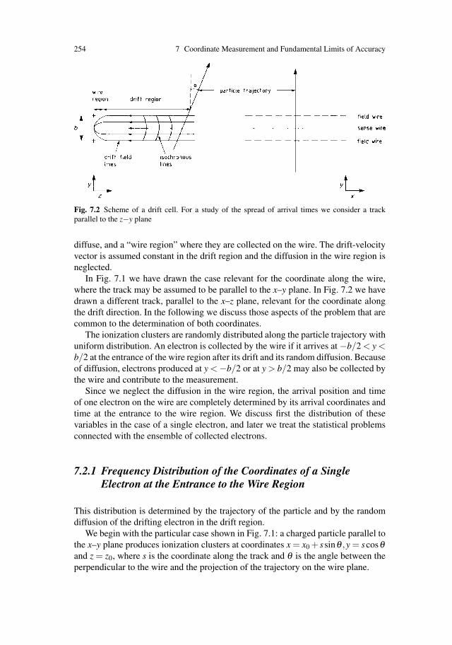
254 7 Coordinate Measurement and Fundamental Limits of Accuracy
Fig. 7.2 Scheme of a drift cell. For a study of the spread of arrival times we consider a trackparallel to the z−y plane
diffuse, and a “wire region” where they are collected on the wire. The drift-velocityvector is assumed constant in the drift region and the diffusion in the wire region isneglected.
In Fig. 7.1 we have drawn the case relevant for the coordinate along the wire,where the track may be assumed to be parallel to the x–y plane. In Fig. 7.2 we havedrawn a different track, parallel to the x–z plane, relevant for the coordinate alongthe drift direction. In the following we discuss those aspects of the problem that arecommon to the determination of both coordinates.
The ionization clusters are randomly distributed along the particle trajectory withuniform distribution. An electron is collected by the wire if it arrives at −b/2 < y <b/2 at the entrance of the wire region after its drift and its random diffusion. Becauseof diffusion, electrons produced at y <−b/2 or at y > b/2 may also be collected bythe wire and contribute to the measurement.
Since we neglect the diffusion in the wire region, the arrival position and timeof one electron on the wire are completely determined by its arrival coordinates andtime at the entrance to the wire region. We discuss first the distribution of thesevariables in the case of a single electron, and later we treat the statistical problemsconnected with the ensemble of collected electrons.
7.2.1 Frequency Distribution of the Coordinates of a SingleElectron at the Entrance to the Wire Region
This distribution is determined by the trajectory of the particle and by the randomdiffusion of the drifting electron in the drift region.
We begin with the particular case shown in Fig. 7.1: a charged particle parallel tothe x–y plane produces ionization clusters at coordinates x = x0 + ssinθ ,y = scosθand z = z0, where s is the coordinate along the track and θ is the angle between theperpendicular to the wire and the projection of the trajectory on the wire plane.

7.2 Basic Formulae for a Single Wire 255
The arrival position of an electron produced at coordinate s along the track is dis-tributed according to a Gaussian diffusion around the production coordinate, whiles is uniformly distributed along the trajectory. Introducing the symbol G,
G(x|〈x〉,σ) =1√
2πσexp
(− (x−〈x〉)2
2σ2
),
to denote the generic Gaussian function of average 〈x〉 and r.m.s. σ we can writedown the frequency distribution of the arrival positions and time of the electron atthe entrance of the wire region (z = zw) as
F(x,y, t)dxdydt =dxdydt
R
+R/2∫
−R/2
ds G(x|x0 + ssinθ ,σx)
× G(y|scosθ ,σy)G(t|(z0 − zw)/u,σt) . (7.1)
Here σx,σy,σt = σz/u denote the diffusion r.m.s. in the three directions (in themost general case we should introduce the diffusion tensor) and u is the drift velocityassumed along z. R is the length of a track arbitrarily chosen so large that Rcosθ � band Rcosθ � σi(i = x,y,z). In the following we will always take the limit R → ∞.
This frequency distribution has been written assuming that just one ionizationelectron is produced along the track segment R. This electron is collected by thewire and contributes to the coordinate measurement only if its arrival position at theentrance to the wire region satisfies the condition −b/2 < y < b/2. The probabilitythat this electron is collected by the wire is
+∞∫−∞
dx
+∞∫−∞
dt
+b/2∫
−b/2
dy F(x,y, t) =b
Rcosθ(7.2)
and is equal to the ratio between the length of the portion of the track between theplanes y = −b/2 and y = b/2 and R.
If we are interested in the measurement of the coordinate along the wire direction(x) alone, the readout electronics will integrate electrons arriving at different times:the probability distribution of the arrival positions at the entrance of the wire regionfor the electrons that are collected by the wire is obtained integrating the distributionF(x,y, t) given by (7.1) in the variable t and normalizing it using (7.2):
fx(x,y)dxdy = dx dycosθ
b
+R/2∫
−R/2
ds G(x|x0 + ssinθ ,σx)G(y|scosθ ,σy) . (7.3)
Assuming that the x coordinate on the wire is the same as at the entrance to thewire region we can compute the average and the variance of the arrival position atthe wire as
256 7 Coordinate Measurement and Fundamental Limits of Accuracy
〈x〉 =
b/2∫
−b/2
dy
+∞∫−∞
x fx(x,y)dx = x0 , (7.4)
〈x2〉−〈x〉2 = σ2x +σ2
y tan2 θ +b2
12tan2 θ . (7.5)
The variance of x is the sum of three terms: the first two depend on diffusion,the third is the projection of the track segment on the wire; this latter we call theangular wire effect. The factor 1/12 that divides the square of the width b of the driftcell comes from the variance of the uniform distribution of the electrons along thetrack.
7.2.2 Frequency Distribution of the Arrival Time of a SingleElectron at the Entrance to the Wire Region
We now turn to the particular case shown in Fig. 7.2: a charged particle parallel tothe y–z plane produces ionization clusters at coordinates x = x0,y = scosα and z =z0 + ssinα , where s is the coordinate along the track and α is the angle between theperpendicular to the drift-velocity direction (z) and the projection of the trajectoryon the wire z–y plane.
The frequency distribution of the arrival positions and time of the electron at theentrance of the wire region (z = zw) is
F(x,y, t)dxdydt =dxdydt
R
+R/2∫
−R/2
dsG(x|x0 +σx)
× G(y|scosα,σy)G(t|(z0 + ssinα − zw)/u,σt) . (7.6)
If we are interested in the measurement of the coordinate along the drift directionz alone, the readout electronics will not distinguish among electrons arriving at dif-ferent wire positions: the probability distribution of the arrival time at the entranceto the wire region for the electrons that are collected by the wire is obtained by inte-grating the distribution given by (7.6) in the variable x and normalizing it using (7.2):
Fz(t,y)dtdy = dtdycosα
b
+R/2∫
−R/2
dsG(t|(z0 + ssinα − zw)/u,σt)
× G(y|scosα,σy) . (7.7)
Assuming for the moment that the arrival time on the wire is equal to the timeat the entrance to the wire region, plus the constant shift zw/u, we can compute theaverage and the variance of the arrival time at the wire;
7.2 Basic Formulae for a Single Wire 257
〈t〉 =
b/2∫
−b/2
dy
+∞∫−∞
t fz(t,y)dt = z0/u , (7.8)
〈t2〉−〈t〉2 = σ2t +
σ2y
u2 tan2 α +b2
12u2 tan2 α . (7.9)
Comparing (7.3) and (7.7) we observe that one can obtain one distribution fromthe other with the substitutions
fx ↔ fz ,
x ↔ z = tu ,
x0 ↔ z0 − zw ,
σx ↔ αz = σtu ,
θ ↔ α .
In the following, we discuss how the cluster fluctuations influence the resolutionin the coordinate measurement along the wire direction (x). This will be done usingthe probability distribution (7.3) and assuming that the x coordinate at the wire isthe same as at the entrance of the wire region. Analogously, the same conclusionscan be drawn with regard to the coordinate measurement in the drift direction, usingthe formal substitutions (7.10). Drift-path variations are introduced in Sect. 7.4.
7.2.3 Influence of the Cluster Fluctuations on the Resolution – theEffective Number of Electrons
Up to this point we have calculated the average and the variance of the position xof a single electron (see (7.4) and (7.5)). For the measurement of the coordinate weaverage over all electrons that are collected by the wire in a given time interval,defined by the readout electronics, and the variance of the coordinate measurementwill be reduced. As it turns out, this reduction is not given by a single factor. This isbecause of the ionization clustering.
We measure the x coordinate averaging the arrival positions of N electrons:
XAV =x1 + x2 + . . .+ xN
N. (7.10)
The variance of XAV depends on the characteristics of the ionization process be-cause the electrons are produced in clusters and therefore the x are, in general, notindependent.
Assume that the N electrons are grouped in M sets of n electrons, each set con-taining the electrons that were produced in the same cluster and after drift and
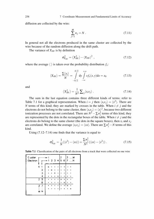
258 7 Coordinate Measurement and Fundamental Limits of Accuracy
diffusion are collected by the wire:
M
∑j=1
n j = N . (7.11)
In general not all the electrons produced in the same cluster are collected by thewire because of the random diffusion along the drift path.
The variance of XAV is by definition
σ2XAV
=⟨X2
AV
⟩−〈XAV〉2 , (7.12)
where the average 〈 〉 is taken over the probability distribution fx:
〈XAV〉 = ∑〈xi〉N
=
b/2∫
−b/2
dy
+∞∫−∞
x fx(x,y)dx = x0 (7.13)
and ⟨X2
AV
⟩=
1N2 ∑i j〈xix j〉 . (7.14)
The sum in the last equation contains three different kinds of terms; refer toTable 7.1 for a graphical representation. When i = j then 〈xix j〉 = 〈x2〉. There areN terms of this kind; they are marked by crosses in the table. When i �= j and theelectrons do not belong to the same cluster, then 〈xix j〉= 〈x〉2, because two differentionization processes are not correlated. There are N2 −∑n2
j terms of this kind, theyare represented by the dots in the rectangular boxes of the table. When i �= j and theelectrons do belong to the same cluster (the dots in the square boxes), then xi and x j
are correlated. We define the average 〈xix j〉= 〈xx〉. There are ∑n2j −N terms of this
kind.Using (7.12–7.14) one finds that the variance is equal to
σ2XAV
=1N
(〈x2〉−〈xx〉)+∑n2
j
N2 (〈xx〉−〈x2〉) . (7.15)
Table 7.1 Classification of the pairs of all electrons from a track that were collected on one wire
7.2 Basic Formulae for a Single Wire 259
In the absence of diffusion, 〈xx〉 is equal to 〈x2〉 and the first term of (7.15) is zero,so we obtain the result derived in Sect. 1.2, where the quantity ∑n2
j/N2 was definedas 1/Neff. If all the clusters consisted of one electron, the term ∑n2
j/N2 there becameequal to 1/N and we obtained the standard formula of the variance of the mean.
We may therefore distinguish the following limiting cases of (7.15):
• Limit of no diffusion, using (7.5):
σ2XAV
→ 1Neff
(〈x2〉−〈x〉2) =1
Neff
b2
12tan2 θ . (7.16)
• Limit of no clustering, using (7.5) and σx = σy = σ :
σ2XAV
→ 1N
(〈x2〉−〈x〉2) =1N
(σ2
cos2 θ+
b2
12tan2 θ
). (7.17)
• Limit θ = 0, in the presence of clustering:
σ2XAV
→ σN
. (7.18)
In (7.16–7.18), Neff is the effective number and N is the total number of elec-trons on the track segment delimited by the cell width; their values are θ -dependentthrough the length of the track segment.
An analytical expression of the covariance 〈xx〉 in (7.15) is derived under certainassumptions in the appendix to this chapter, resulting in formula (7.81) for σ2
XAV.
This can be rewritten in the form
σ2XAV
→ 1N′
σ2
cos2 θ+
1N′
eff
b2
12tan2 θ . (7.19)
where the quantities N′ and N′eff depend on θ as well as on σ and b.
Let us first deal with the term proportional to (b2/12) tan2 θ . We may regard N′eff
as the effective number of electrons that would cause the same fluctuation as thecombined action of ionization plus diffusion, thus extending the original meaningof Neff defined in Sect. 1.2 and used in (7.16).
The quantity N′eff, for which an analytic expression is given in the
appendix to this chapter, can also be calculated with a numerical simulation of theionization and diffusion process. In order to compute it as a function of the diffusionparameter σ we evaluate the variance VAV of the average of the coordinates alongthe track direction of those electrons that, after diffusion σ along the track direction,are contained in a track segment of length l. We write
1N′
eff
1Neff(σ)
=l2
121
VAV(σ). (7.20)
Figure 7.3 shows how Neff(σ) varies with diffusion. We have plotted on the ver-tical axis the quantity
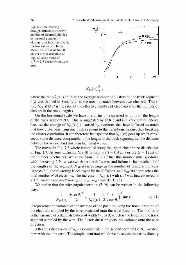
260 7 Coordinate Measurement and Fundamental Limits of Accuracy
Fig. 7.3 Declusteringthrough diffusion: effectivenumber of electrons dividedby the total number ofclusters, as a function of σ/l,for two values of l. In theMonte Carlo calculation thecluster-size distribution ofFig. 1.7 and a value of1/λ = 2.7 clusters/mm wereused
Neff(σ)λl
,
where the ratio λ/l is equal to the average number of clusters on the track segmentl (λ was defined in Sect. 1.1.1 as the mean distance between two clusters). There-fore Neff(σ)λ/l is the ratio of the effective number of electrons over the number ofclusters in the track length l.
On the horizontal scale we have the diffusion expressed in units of the lengthof the track segment σ/l. This is suggested by (7.81) and is a very natural choicebecause the change of Neff(σ) is caused by electrons that have diffused so muchthat they cross over from one track segment to the neighbouring one, thus breakingthe cluster correlation. It can therefore be expected that Neff(σ) goes up when σ ex-ceeds some distance comparable to the length of the track segment, i.e. the distancebetween the wires. And this is in fact what we see.
The curves in Fig. 7.3 where computed using the argon cluster-size distributionof Fig. 1.7. At zero diffusion Neff(0) is only 0.3(l = 0.4cm) or 0.2 (l = 1cm) ofthe number of clusters. We know from Fig. 1.19 that this number must go downwith increasing l. Now we switch on the diffusion, and before σ has reached halfthe length l of the segment, Neff(σ) is as large as the number of clusters. For verylarge σ/l all the clustering is destroyed by the diffusion, and Neff(σ) approaches thetotal number N of electrons. The increase of Neff(σ) with σ/l was first observed ina TPC and termed declustering through diffusion [BLU 86].
We notice that the wire angular term in (7.19) can be written in the followingway:
1Neff(σ)
(b tanθ)2
12=
1Neff(σ)
112
(b
cosθ
)2
sin2 θ . (7.21)
It represents the variance of the average of the position along the track direction ofthe electrons sampled by the wire, projected onto the wire direction. The first termis the variance of a flat distribution of width b/cosθ , which is the length of the tracksegment sampled by the wire. The factor sin2 θ projects this variance onto the wiredirection.
After this discussion of N′eff as contained in the second term of (7.19), we deal
now with the first term. The simple form into which we have cast the terms directly
7.3 Accuracy in the Measurement of the Coordinate 261
proportional to σ2 (cf. (7.81)) hides the complications in the symbol N′. Although itis true that in the limiting cases of (7.17) and (7.18) N′ is exactly equal to N, the totalnumber of electrons on the track segment delimited by the cell width, N′ changesas a function of θ ,σ and b so as to make the variance σ2
XAVlarger. The physical
cause of this is the rare larger clusters outside the cell that send some electrons viadiffusion to the edge of the cell, and more so when θ is large. We have two reasonsnot to go into these details here. When we omit the primes in (7.19) the omissionsamount to less than 25% in the quantity σXAV (except in extreme cases). The omittedparts, which pull measurements to one side in our cell, have a tendency to pull thecorresponding measurement in the neighbouring cell to the opposite side. Thereforeit is better to leave them out when combining several cells. The contributions ofseveral wires are discussed in Sects. 7.3 and 7.4.
In conclusion we simplify (7.19) to read
σ2XAV
=1N
σ2
cos2 θ+
1Neff
b2
12tan2 θ . (7.22)
It represents the square of the accuracy with which a track coordinate XAV (7.10)can be measured along a single wire in the absence of a magnetic field.
7.3 Accuracy in the Measurement of the Coordinatein or near the Wire Direction
7.3.1 Inclusion of a Magnetic Field Perpendicular to the WireDirection: the Wire E ××× B Effect
Drift chambers with precise measurements of the track coordinates along the wiredirection are often operated with a magnetic field perpendicular to the direction ofthe wires. With this configuration one can obtain a precise determination of the cur-vature induced on the particle trajectory by the magnetic field, and the momentumof the particle can be determined (see Chap. 8 for details).
The presence of a magnetic field perpendicular to the wire direction modifies theangular wire term of the variance of the arrival position of the electrons (7.5). Itbecomes asymmetric and, on average, larger because the track segment is projectedonto the wire in a more complicated way. The electrons that after their drift arecollected in the cylindrical field of the wire have to move transverse to the magneticfield (Fig. 7.4). This produces an E × B force according to (2.6) and causes theelectrons to drift under an effective angle ψ toward the wire. The angle ψ is suchthat tanψ = ωτ , where ω is the cyclotron frequency and τ is the time between twoelectron collisions suitably averaged. Details have been treated in Sect. 2.1.
The arrival position xw of an electron entering the region close to the wirewith coordinates x and y is xw = x− y tanψ; the variance of xw on the frequencydistribution (7.3) is

262 7 Coordinate Measurement and Fundamental Limits of Accuracy
Fig. 7.4 (a) Directions of theelectric and magnetic fields inthe region close to the sensewire. The magnetic fieldpoints into the page. (b)Direction of the drift velocityof the electrons in this regionprojected onto the x–y plane
〈x2w〉−〈xw〉2 =
σ2
cos2 θ+
b2
12(tanθ − tanψ)2 . (7.23)
The electrons produced by a track at θ = 0 are spread over a region b tanψ , andthose of a track at an arbitrary angle are smeared over a distance b(tanθ − tanψ).The width of the charge distribution on the wire has a minimum at θ = ψ and not atθ = 0.
This effect was discovered with the TRIUMF-TPC [HAR 84] and is typically themost important limitation of the measuring accuracy in all TPC-like detectors usinga gas with high values of ωτ . In the TRIUMF-TPC the angle ψ was 29◦, and 32◦ inthe ALEPH TPC in standard running conditions. The broadening of the avalanchewidth has been systematically studied in [BLU 86].
Using (7.23) we can rewrite (7.22) to include this effect:
σ2XAV
=1N
σ2
cos2 θ+
1Neff
b2
12(tanθ − tanψ)2 . (7.24)
Equation (7.24) is the general expression for the accuracy σXAV with which atrack segment can be measured on one wire along the wire direction. Summa-rizing our findings up to here, we see that this accuracy depends on the pro-jected angle θ the track has with respect to the normal to the wire direction aswell as on the angle ψ of the wire E × B effect. Neff is roughly 6 for 1 cm ofargon NTP and is more accurately obtained in Figs. 7.3 and 1.19. The diffu-sion term is characterized by the width σ of the single-electron diffusion trans-verse to the drift and the total number N of electrons, typically 100/cm in argonNTP.
The size and relative importance of the two terms in (7.24) depend on the electrondrift length L, because σ2 is proportional to L and Neff depends on L through thedeclustering effect (Fig. 7.3). Also the angle θ has some influence on N and Neff asthe length of the track segment varies with θ . If one wants to be more specific, onehas to take into account the details of a particular chamber.

7.3 Accuracy in the Measurement of the Coordinate 263
7.3.2 Case Study of the Explicit Dependence of the Resolutionon L and θ
Writing (7.24) in the form
σ2XAV
=1n0
(C2L
bcosθ+
b12
(tanθ tanψ)2 cosθg(L)
)(7.25)
we have introduced the L dependence of the diffusion and of Neff:
σ2 = C2L , (7.26)
Neff = Ng(L) , (7.27)
as well as the θ dependence of N:
N = n0b/cosθ . (7.28)
Here n0 is the number of collected electrons per unit track length. (We recallthat g(L) is not a universal function but depends to some extent on N,band θ .)
Figure 7.5a-c shows σ2XAV
calculated as a function of L at θ = 0 for C2 = 3.4×10⁻³ mm, ψ = 32◦ (corresponding to a gas mixture of 80% argon and 20% methanein a field of 0.85 T), b = 4mm, n0 = 8.1electrons/mm. We notice that the resolu-tion goes through a shallow minimum at small L and is dominated by diffusion atlarge L.
Figure 7.6 shows σ2XAV
as a function of the angle θ for two different values of Land for the same choice of the other parameters.
Fig. 7.5a-c Variance of theaverage arrival position as afunction of the drift length atθ = 0 – the special casedescribed in the text. (a)Contribution of the diffusion;(b) contribution of theangular wire effect; (c) sumof the two
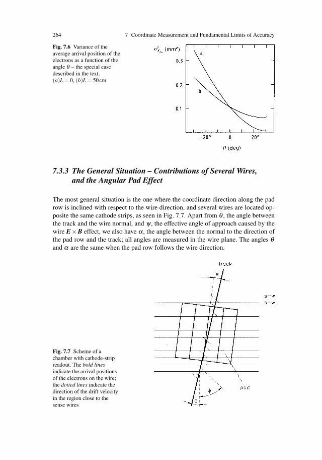
264 7 Coordinate Measurement and Fundamental Limits of Accuracy
Fig. 7.6 Variance of theaverage arrival position of theelectrons as a function of theangle θ – the special casedescribed in the text.(a)L = 0, (b)L = 50cm
7.3.3 The General Situation – Contributions of Several Wires,and the Angular Pad Effect
The most general situation is the one where the coordinate direction along the padrow is inclined with respect to the wire direction, and several wires are located op-posite the same cathode strips, as seen in Fig. 7.7. Apart from θ , the angle betweenthe track and the wire normal, and ψ , the effective angle of approach caused by thewire E×B effect, we also have α , the angle between the normal to the direction ofthe pad row and the track; all angles are measured in the wire plane. The angles θand α are the same when the pad row follows the wire direction.
Fig. 7.7 Scheme of achamber with cathode-stripreadout. The bold linesindicate the arrival positionsof the electrons on the wire;the dotted lines indicate thedirection of the drift velocityin the region close to thesense wires

7.3 Accuracy in the Measurement of the Coordinate 265
The signals induced in a cathode strip are from k wires, wherek = pad length h/wire pitch b.
These signals are added in the measuring process. We want to compute the achiev-able accuracy. As the situation is quite complicated we wish to start with a simplecase. The basic statistical relation will be derived for the special geometry given byα = 0, θ = 0; also we will assume σ = 0. Later on we will generalize our findingsstep by step.
The simplified geometry is sketched in Fig. 7.8. The ionization clusters along thetrack are redistributed onto the sense wires, where they occupy sections of lengthb tanψ . The situation is quite similar to the one in Sect. 1.2.6, where we treated theproblem of charge localization along a track. The coordinate to be determined bythe pads in one measurement is
XAVP =∑m1
i=1 xini +∑m2i=m1+1 xini + . . .+∑mk
i=mk−1+1 xini(∑mk
i=1 ni)2 , (7.29)
where each xi is the position of a cluster with ni electrons; there are m1 clusterson the first, and m j −m j−1 on the jth sense wire ( j = 1, . . . ,k). Averaging over thepositions xi – which are distributed between −(b/2) tanψ and +(b/2) tanψ – wefind for the average and the variance
〈XAVP〉 = 0
and
σ2AVP =
⟨X2
AVP
⟩−〈XAVP〉2
=b2 tan2 ψ
12∑mk
i=1 n2i(
∑mki=1 ni
)2 (7.30)
σ2AVP =
b2 tan2 ψ12
1Neff(h)
(α = θ = σ = 0) .
Fig. 7.8 Track and sensewires for (7.30)

266 7 Coordinate Measurement and Fundamental Limits of Accuracy
Here we have denoted by 1/Neff(h) the statistical factor which is equal to the sumof the squared cluster size divided by the square of the summed cluster sizes, takenover all the clusters on the piece of track that is delimited by the pad length h. Let usrepeat (cf. Sect. 1.2.9 that the effective number Neff is a measure of fluctuation whichis smaller than the number of clusters because of the fluctuations of the cluster size.It is not proportional to h; for argon it scales according to Fig. 1.22. ComparingNeff(b), the corresponding number that belongs to a wire cell, we have for that case
Neff(h) ∼ Neff(b)(h/b)0.54 .
For this reason the achievable accuracy of pads does not improve with the squareroot but (for argon) more with the fourth root of the pad length.
In the next step we let θ and σ be different from zero, but keep σ b and α = 0.The geometry is sketched in Fig. 7.9. The angle θ the track makes with the wire nor-mal has two consequences: it changes the length on the wire occupied by charges,from b tan ψ to b(tanψ − tanθ), and it introduces the projection factor cosθ be-tween this length and the coordinate direction. The diffusion, finally, contributes tothe variance the same term as in (7.22) but with two changes. Firstly, the projectionfactor onto the coordinate direction is 1 in the present case. Secondly, N now repre-sents the total number of electrons from the track segment delimited by h; we writeN(h), which is of course proportional to h. The variance of XAVP therefore assumesthe form
σ2XAVP
=σ2
N(h)+
1Neff(h)
b2
12(tanψ − tanθ)2 cos2 θ(α = 0,σ b). (7.31)
Next we let α assume a non-zero value. This has the consequence that the twoprojection factors must be referred to the new coordinate direction, that is the dif-fusion term receives in its denominator the factor cos2 α , and the projection factorof the angular term changes into cos2(θ −α). The variance (7.31) of XAVP receivesanother contribution, which describes the fluctuation of the position of the centre of
Fig. 7.9 Track and sensewires for (7.31)
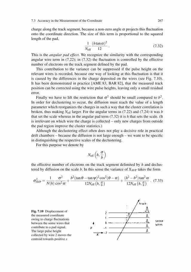
7.3 Accuracy in the Measurement of the Coordinate 267
charge along the track segment, because a non-zero angle α projects this fluctuationonto the coordinate direction. The size of this term is proportional to the squaredlength of the pad,
1Neff
(h tanα)2
12. (7.32)
This is the angular pad effect. We recognize the similarity with the correspondingangular wire term in (7.22); in (7.32) the fluctuation is controlled by the effectivenumber of electrons on the track segment defined by the pad.
This contribution to the variance can be suppressed if the pulse height on therelevant wires is recorded, because one way of looking at this fluctuation is that itis caused by the differences in the charge deposited on the wires (see Fig. 7.10).It has been demonstrated in practice [AME 83, BAR 82], that the measured trackposition can be corrected using the wire pulse heights, leaving only a small residualerror.
Finally we have to lift the restriction that σ2 should be small compared to b2.In order for declustering to occur, the diffusion must reach the value of a lengthparameter which reorganizes the charges in such a way that the cluster correlation isbroken, thus making Neff larger. For the angular terms in (7.22) and (7.24) it was bthat set the scale whereas in the angular pad term (7.32) it is h that sets the scale. (Itis irrelevant on which wire the charge is collected – only new charges from outsidethe pad region improve the cluster statistics.)
Although the declustering effect often does not play a decisive role in practicaldrift chambers – because the diffusion is not large enough – we want to be specificin distinguishing the respective scales of the declustering.
For this purpose we denote by
Neff
(h,
σb
)
the effective number of electrons on the track segment delimited by h and declus-tered by diffusion on the scale b. In this sense the variance of XAVP takes the form
σ2AVP =
1N(h)
σ2
cos2 α+
b2(tanθ − tanψ)2 cos2(θ −α)12Neff
(h, σ
b
) +(h2 −b2) tan2 α
12Neff(h, σ
h
) . (7.33)
Fig. 7.10 Displacement ofthe measured coordinateowing to charge fluctuationsbetween the sense wires thatcontribute to a pad signal.The large pulse heightcollected by wire 2 moves thecentroid towards positive x

268 7 Coordinate Measurement and Fundamental Limits of Accuracy
This is the principal limit of the coordinate measuring accuracy using pads; θ ,ψ ,and α were defined in Fig. 7.7. In the usual case of no declustering, the values ofNeff for argon can be taken from Fig. 1.22.
7.3.4 Consequences of (7.33) for the Construction of TPCs
The relative size of the three terms in (7.33) depends, firstly, on the diffusion of theelectrons during their drift. In the presence of a typical longitudinal magnetic field,the magnetic anisotropy of diffusion will make the first term the smallest one onaverage, for any practical choice of b and h.
In the usual case, a pad extends over several wires, and h is much larger than b;therefore the third term will dominate even for a small α . The most critical coordi-nate measurements are those for a determination of large track momenta on trackswith a small curvature. The pad rows should therefore be oriented at right angles tothese critical tracks, so that, for them, α ≈ 0. For this reason, the ALEPH and theDELPHI TPCs have circular pad rows.
With the choice of h the designer of the TPC wants to take advantage of thefact that N(h) increases in proportion to h and Neff(h) approximately in proportionto
√h. Also, the larger the collected amount of charge on a pad the less critical is
the noise of the electronic amplifier. On the other hand the third term in (7.33) canbe kept small only within a range of α which becomes smaller and smaller as his increased. Even the modest magnetic bending of a high-momentum track mayexceed this range if h is made too large. It can be shown that the consequence isa constant limiting relative-momentum-measuring accuracy δ p/p rather than onewhich decreases as p is reduced.
Problems of double-track resolution are discussed in Sect. 11.7.1
7.3.5 A Measurement of the Angular Variation of the Accuracy
The second term in (7.33) can be studied in detail by measuring σ2AVP as a function
of θ , keeping α fixed at 0. This has been done by Blum et al. [BLU 86] using a smallTPC with rotatable wires in a beam of 50 GeV muons. Each track had its transverseposition measured at four points using the pulse heights on the pads (see Fig. 7.11).The pad length h was 3 cm and the wire pitch b was 4 mm. The variance was deter-mined for every track as one half the sum of the squared residuals of the straight-linefit. The result is σ2
m, the measured variance averaged over many tracks, as a functionof the angle θ between the tracks and the normal to the wires. According to (7.33)σ2
m should vary as
σ2m = σ2
0 +b2
12Neff(h, σ
b
) (tanθ − tanψ)2 cos2 θ
= σ20 +
b2
12Neff(h, σ
b
) sin2(θ −ψ)cos2 ψ
, (7.34)

7.3 Accuracy in the Measurement of the Coordinate 269
Fig. 7.11 Layout of TPC with rotatable wires [BLU 86]
where σ20 contains the effects of diffusion and, perhaps, of the electronics and any
remaining contribution of the angular pad effect.The results are depicted in Fig. 7.12a,b. The curves represent fits to (7.34) on ad-
justing the three free parameters ψ,σ0 and Neff(h,σ/b). A reversal of the magneticfield changes the sign of ψ so that two curves are seen in Fig. 7.12a,ba. The valuesof the fitted parameters are shown in Table 7.2.
Keeping in mind that a magnetic field of 1.5 T reduces the transverse diffu-sion coefficient by a factor 50 (cf. Sect. 2.4.5) we expect for the mean squarewidth of the diffusion cloud after 4 cm of drift a value of 1.6mm2(B = 0) or3.2×10−2 mm2(B = 1.5T). Since on a pad length of 3 cm the number of ionization
Fig. 7.12a,b The square of the measuring accuracy σ determined by [BLU 86] as a function ofthe track angle θ ,(a) in a magnetic field of ±1.5 T, (b) without magnetic field. The continuouslines were calculated using (7.34) with the fitted parameters of Table 7.2
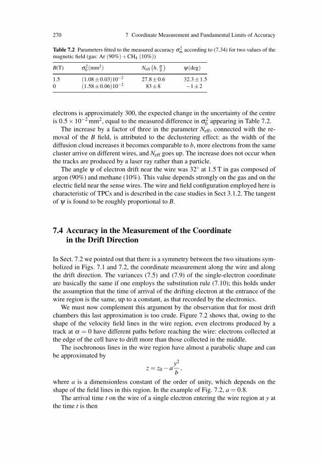
270 7 Coordinate Measurement and Fundamental Limits of Accuracy
Table 7.2 Parameters fitted to the measured accuracy σ 2m according to (7.34) for two values of the
magnetic field (gas: Ar (90%)+CH4 (10%))
B(T) σ20 (mm2) Neff
(h, σ
b
)ψ(deg)
1.5 (1.08±0.03)10−2 27.8±0.6 32.3±1.50 (1.58±0.06)10−2 83±8 −1±2
electrons is approximately 300, the expected change in the uncertainty of the centreis 0.5×10⁻² mm2, equal to the measured difference in σ2
0 appearing in Table 7.2.The increase by a factor of three in the parameter Neff, connected with the re-
moval of the B field, is attributed to the declustering effect: as the width of thediffusion cloud increases it becomes comparable to b, more electrons from the samecluster arrive on different wires, and Neff goes up. The increase does not occur whenthe tracks are produced by a laser ray rather than a particle.
The angle ψ of electron drift near the wire was 32◦ at 1.5 T in gas composed ofargon (90%) and methane (10%). This value depends strongly on the gas and on theelectric field near the sense wires. The wire and field configuration employed here ischaracteristic of TPCs and is described in the case studies in Sect 3.1.2. The tangentof ψ is found to be roughly proportional to B.
7.4 Accuracy in the Measurement of the Coordinatein the Drift Direction
In Sect. 7.2 we pointed out that there is a symmetry between the two situations sym-bolized in Figs. 7.1 and 7.2, the coordinate measurement along the wire and alongthe drift direction. The variances (7.5) and (7.9) of the single-electron coordinateare basically the same if one employs the substitution rule (7.10); this holds underthe assumption that the time of arrival of the drifting electron at the entrance of thewire region is the same, up to a constant, as that recorded by the electronics.
We must now complement this argument by the observation that for most driftchambers this last approximation is too crude. Figure 7.2 shows that, owing to theshape of the velocity field lines in the wire region, even electrons produced by atrack at α = 0 have different paths before reaching the wire: electrons collected atthe edge of the cell have to drift more than those collected in the middle.
The isochronous lines in the wire region have almost a parabolic shape and canbe approximated by
z = z0 −ay2
b,
where a is a dimensionless constant of the order of unity, which depends on theshape of the field lines in this region. In the example of Fig. 7.2, a = 0.8.
The arrival time t on the wire of a single electron entering the wire region at y atthe time t is then
7.4 Accuracy in the Measurement of the Coordinate in the Drift Direction 271
t = t ′ +1u
(zw +a
y2
b
). (7.35)
The average and variance of this last expression on the distribution (7.7) are
〈t〉 =1u
(z0 +a
b12
), (7.36)
〈t2〉−〈t〉2 =1u2
(σ2
z +σ2y tan2 α +
b2
12tan2 α +
a2b2
180
), (7.37)
where the last and new term is the contribution of the drift-path variations in thewire region.
7.4.1 Inclusion of a Magnetic Field Parallel to the Wire Direction:the Drift E×B Effect
Drift chambers with precise measurements of the track coordinates along the driftdirection are often operated with a magnetic field perpendicular to the drift directionand parallel to the wires. With this configuration one can obtain a precise determi-nation of the curvature induced on the particle trajectory by the magnetic field, andthe momentum of the particle can be determined (see Chap. 8 for details).
If a magnetic field perpendicular to the drift electric field is present, the driftingelectrons have to move transverse to it. This produces an E×B force according to(2.6) and causes the electrons to drift under an effective angle ψ with respect to thedirection of the electric field. The angle ψ is such that tanψ = ωτ , where ω is thecyclotron frequency and τ is the time between two collision suitably averaged.
Electrons produced by a track at α = 0 do not arrive simultaneously at the en-trance to the wire region, but their arrival positions depend linearly on y with a slopetan ψ .
The variance of the arrival time of a single electron depends now on the angle ψ:
〈t2〉−〈t〉2 =1u2
(σ2
z +σ2y tan2 α +
b2
12(tanα − tanψ)2 +
a2b2
180
), (7.38)
where the diffusion parameter σz refers to the new drift direction, and σy to thedirection perpendicular to it and to the magnetic field. The two parameters are notnecessary equal, owing to the electric anisotropy of diffusion (cf. Sect. 2.2.5), butfor simplicity we will replace them below by a common value.
Up to now we have dealt with the drift-time variations of a single electron. Whena measurement is performed, the whole swarm arrives. There are various ways toextract the time information. In terms of electronics, one may either employ discrim-inators of various types in order to trigger on the first electrons, or on the centroidof the pulse or on some other value based on a threshold-crossing time. Or one mayapply a very fast sampling technique in order to obtain a numerical representation of
272 7 Coordinate Measurement and Fundamental Limits of Accuracy
the pulse shape, which may be used to derive a suitable estimator. We discuss heretwo estimators of the arrival time of the swarm: the average and the Mth electron,assuming for simplicity ψ = 0.
7.4.2 Average Arrival Time of Many Electrons
When we average over the arrival times of all the electrons, the statistical reductionof the different terms of (7.38) is not the same because of the correlation betweenelectrons produced in the same cluster. Following the lines of Sect. 7.2 we can writethe variance of the average arrival time as
σ2TAV =
1u2
[1N
σ2
cos2 α+
1Neff
(b2
12tan2 α +
a2b2
180
)], (7.39)
where N represents the total ionization collected by the wire, and Neff is the effectivenumber of independent electrons.
The contribution of the drift-path variation of the variance of the average is al-ways present, even for tracks in good geometry (α = 0) and close to the wire(σ ≈ 0). It is quite large and increases with b more than linearly, since Neff increaseswith the track length more slowly than in proportion.
Obviously the average over all arrival times fluctuates so badly because of thelate-arriving electrons, those that have to take the longest path when they approachthe wire. If one derives the time signal from the few electrons that arrive first, thelatecomers do not contribute. In fact, a discriminator with a low threshold will dothis automatically.
7.4.3 Arrival Time of the Mth Electron
Let the time signal be defined by the moment that the Mth electron arrives. Here Mcan either be a fixed number (this is the case when a fixed-threshold discriminatoris used) or a given fraction of the total number of electrons contributing (this is thecase of a constant-fraction discriminator).
The probability p(t) of one electron arriving before the time t is calculable using(7.7) and (7.35):
p(t) =∫ t−∞ f (τ)dτ∫ +∞−∞ f (τ)dτ
, (7.40)
where
f (τ)dτ =
+b/2∫
−b/2
dy fz(τ − (zw +ay2/b)/u,y)dτ . (7.41)
Next we have to write out the probability R(t) that the Mth electron out of agroup of N arrives in the interval dt. It is equal to the probability that any one of

7.4 Accuracy in the Measurement of the Coordinate in the Drift Direction 273
the N electrons arrives precisely in dt (equal to N (dp/dt) or N dp) multiplied by theprobability that any of (M − 1) out of the (N − 1) remaining ones arrives before tand the rest after t +dt:
R(t)dt = N
(N −1
M−1
)pM−1(1− p)N−M dp
dtdt
= M
(N
M
)pM−1(1− p)N−Mdp = P(p)dp. (7.42)
In the last expression we have defined a probability density P(p) for the variable p.It is easy to show that
+∞∫−∞
R(t)dt =1∫
0
P(p)dp = 1 .
Here and in the following steps we make use of the well-known expression forthe definite integral
1∫0
xk(1− x) jdx =j!k!
( j + k +1)!.
The variance of the arrival time of the Mth electron is given by
σ2TM = 〈t2〉−〈t〉2 ,
with
〈t2〉 =+∞∫
−∞
t2R(t)dt =1∫
0
t2(p)P(p)dp
and
〈t〉 =+∞∫
−∞
tR(t)dt =1∫
0
t(p)P(p)dp . (7.43)
The function t(p) is obtained by inverting (7.40).We consider now separately the two contributions of the difference of the drift
paths and of the diffusion and study the particular case of a track perpendicular tothe drift velocity direction (α = 0).
7.4.4 Variance of the Arrival Time of the Mth Electron:Contribution of the Drift-Path Variations
In order to study the effect of the drift-path variation alone we go to the limitσy → 0,σt → 0 of (7.41) at α = 0, and obtain
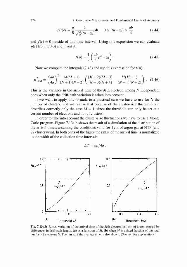
274 7 Coordinate Measurement and Fundamental Limits of Accuracy
f (t)dt =uR
1√ab (tu− z0)
dt, 0 ≤ (tu− z0) ≤ab4
(7.44)
and f (t) = 0 outside of this time interval. Using this expression we can evaluatep(t) from (7.40) and invert it:
t(p) =1u
(ab4
p2 + z0
). (7.45)
Now we compute the integrals (7.43) and use this expression for t(p):
σ2TPM =
(ab4u
)2 M(M +1)(N +1)(N +2)
((M +2)(M +3)(N +3)(N +4)
− M(M +1)(N +1)(N +2)
). (7.46)
This is the variance in the arrival time of the Mth electron among N independentones when only the drift-path variation is taken into account.
If we want to apply this formula to a practical case we have to use for N thenumber of clusters, and we realize that because of the cluster-size fluctuations itdescribes correctly only the case M = 1, since the threshold can only be set at acertain number of electrons and not of clusters.
In order to take into account the cluster-size fluctuations we have to use a MonteCarlo program. Figure 7.13a,b shows the result of a simulation of the distribution ofthe arrival times, assuming the conditions valid for 1 cm of argon gas at NTP (and27 clusters/cm). In both parts of the figure the r.m.s. of the arrival time is normalizedto the width of the collection time interval:
ΔT = ab/4u .
Fig. 7.13a,b R.m.s. variation of the arrival time of the Mth electron in 1 cm of argon, caused bydifferences in drift-path length, (a) as a function of M, (b) when M is a fixed fraction of the totalnumber of electrons N. The r.m.s. of the average time is also shown. (See text for explanations.)

7.4 Accuracy in the Measurement of the Coordinate in the Drift Direction 275
Also visible is the r.m.s. of the average (7.39), evaluated for α = 0,σ = 0, Neff = 6and normalized to the same quantity. We observe that the limit of the accuracy dueto the drift-path variation can be made very small by lowering the threshold. Forexample, σTM comes down to 30% of σTAV when triggering on a value of M equalto 5% of N. But by gaining on the drift-path variations, one loses on the diffusionterm.
7.4.5 Variance of the Arrival Time of the Mth Electron:Contribution of the Diffusion
Next we study the contribution of diffusion. The probability density f (t) of (7.41)with a = 0 and α = 0 takes the form
f (t)dt =bR
exp
(− (t− z0
u )2
2σ2t
)√
2πσtdt , (7.47)
and the function p(t) of (7.40) is the function E:
p(t) = E
(t − z0/u
σt
)=
t−z0/uσt∫
−∞
dqexp(−q2/2)√
2π. (7.48)
To compute the variance of the arrival time of the Mth electron we should solvethe integrals (7.43) using the function t(p) defined by the inverse of (7.40).
Since we cannot invert the expression (7.48) analytically, we linearize it in thevicinity of the average value of the function P(p) of (7.42). This procedure is justi-fied by the fact that the variance of the function P(p) is small when M is small and Nlarge. It is illustrated in Fig. 7.14. The variance of the arrival time is the variance ofp on the probability distribution P(p) projected onto the t axis using the derivative
dtdp
= σtdq
dE(q)= σt
√2π exp
(+〈q〉2
2
),
evaluated at 〈q〉 defined by 〈p〉 = E(〈q〉).The variance of p is given by
〈p2〉 =1∫
0
p2P(p)dp =M
N +1
and
〈p2〉 =1∫
0
p2P(p)dp =M(M +1)
(N +1)(N +2),

276 7 Coordinate Measurement and Fundamental Limits of Accuracy
Fig. 7.14 Illustration of(7.50): the variance of p isprojected onto the time axisusing the tangent to the errorfunction erf(t) in order toobtain σTDM
from which we obtain
〈p2〉−〈p〉2 =M
(N +1)(N +2)
(1− M
N +1
)≈ M
N2
(1− M
N
). (7.49)
Projecting now this variance onto the time axis (see Fig. 7.14) we obtain
σ2TDM ≈ σ2
t
N2π exp(〈q〉2)
MN
(1− M
N
), (7.50)
where 〈q〉 is the normalized average arrival time, given by the condition that thecorresponding integral probability p takes on the value M/(N + 1), or in good ap-proximation, M/N. In other words, 〈q〉 is given by the inverse of the function E atits argument M/N :
〈q〉 = E−1(M/N) . (7.51)
Expression (7.50) with (7.51) represents the answer to the question how much thearrival time of the Mth electron fluctuates when each single electron has a Gaussiandistribution with a width σt ;σTDM goes down with the total number N of electronsand is equal to σt/
√N times a factor which depends only on M/N. The factor de-
scribes the loss of accuracy when the arrival-time measurement is based on the Mthelectron rather than on the average of all N. (The variance σ2
TAV of the average ar-rival time caused by diffusion alone was σ2
t /N as implied by (7.39).) The loss factoris plotted in Fig. 7.15 and is seen to be always larger than 1. For example the loss isa factor 2 if one triggers on the first 5% of the swarm.
An often-quoted formula according to which
σTDM =σt√
2logN
∞
∑r=M
1r2 (7.52)
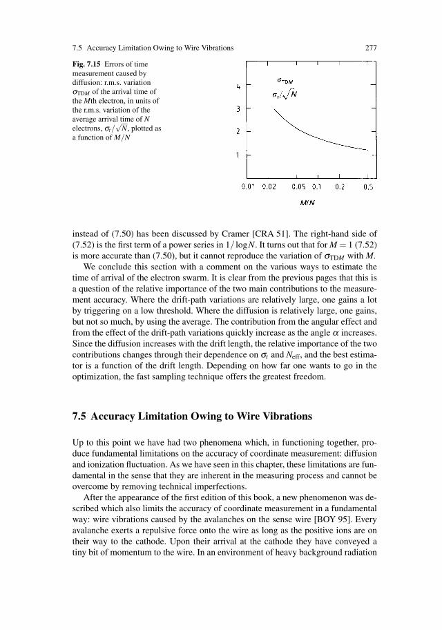
7.5 Accuracy Limitation Owing to Wire Vibrations 277
Fig. 7.15 Errors of timemeasurement caused bydiffusion: r.m.s. variationσTDM of the arrival time ofthe Mth electron, in units ofthe r.m.s. variation of theaverage arrival time of Nelectrons, σt/
√N, plotted as
a function of M/N
instead of (7.50) has been discussed by Cramer [CRA 51]. The right-hand side of(7.52) is the first term of a power series in 1/ logN. It turns out that for M = 1 (7.52)is more accurate than (7.50), but it cannot reproduce the variation of σTDM with M.
We conclude this section with a comment on the various ways to estimate thetime of arrival of the electron swarm. It is clear from the previous pages that this isa question of the relative importance of the two main contributions to the measure-ment accuracy. Where the drift-path variations are relatively large, one gains a lotby triggering on a low threshold. Where the diffusion is relatively large, one gains,but not so much, by using the average. The contribution from the angular effect andfrom the effect of the drift-path variations quickly increase as the angle α increases.Since the diffusion increases with the drift length, the relative importance of the twocontributions changes through their dependence on σt and Neff, and the best estima-tor is a function of the drift length. Depending on how far one wants to go in theoptimization, the fast sampling technique offers the greatest freedom.
7.5 Accuracy Limitation Owing to Wire Vibrations
Up to this point we have had two phenomena which, in functioning together, pro-duce fundamental limitations on the accuracy of coordinate measurement: diffusionand ionization fluctuation. As we have seen in this chapter, these limitations are fun-damental in the sense that they are inherent in the measuring process and cannot beovercome by removing technical imperfections.
After the appearance of the first edition of this book, a new phenomenon was de-scribed which also limits the accuracy of coordinate measurement in a fundamentalway: wire vibrations caused by the avalanches on the sense wire [BOY 95]. Everyavalanche exerts a repulsive force onto the wire as long as the positive ions are ontheir way to the cathode. Upon their arrival at the cathode they have conveyed atiny bit of momentum to the wire. In an environment of heavy background radiation
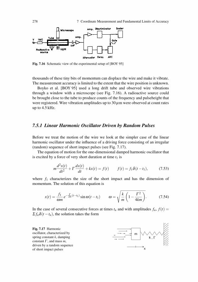
278 7 Coordinate Measurement and Fundamental Limits of Accuracy
Fig. 7.16 Schematic view of the experimental setup of [BOY 95]
thousands of these tiny bits of momentum can displace the wire and make it vibrate.The measurement accuracy is limited to the extent that the wire position is unknown.
Boyko et al. [BOY 95] used a long drift tube and observed wire vibrationsthrough a window with a microscope (see Fig. 7.16). A radioactive source couldbe brought close to the tube to produce counts of the frequency and pulseheight thatwere registered. Wire vibration amplitudes up to 30 μm were observed at count ratesup to 4.5 kHz.
7.5.1 Linear Harmonic Oscillator Driven by Random Pulses
Before we treat the motion of the wire we look at the simpler case of the linearharmonic oscillator under the influence of a driving force consisting of an irregular(random) sequence of short impact pulses (see Fig. 7.17).
The equation of motion for the one-dimensional damped harmonic oscillator thatis excited by a force of very short duration at time t1 is
md2x(t)
dt2 +Γdx(t)
dt+ kx(t) = f (t) f (t) = f1δ (t − t1), (7.53)
where f1 characterizes the size of the short impact and has the dimension ofmomentum. The solution of this equation is
x(t) =f1
ωme−
Γ2m (t−t1) sinω(t − t1) ω =
√km
(1− Γ 2
4km
). (7.54)
In the case of several consecutive forces at times tn and with amplitudes fn, f (t) =Σ fnδ (t − tn), the solution takes the form
Fig. 7.17 Harmonicoscillator, characterized byspring constant k, dampingconstant Γ , and mass m,driven by a random sequenceof short impact pulses
mk , Γ
x
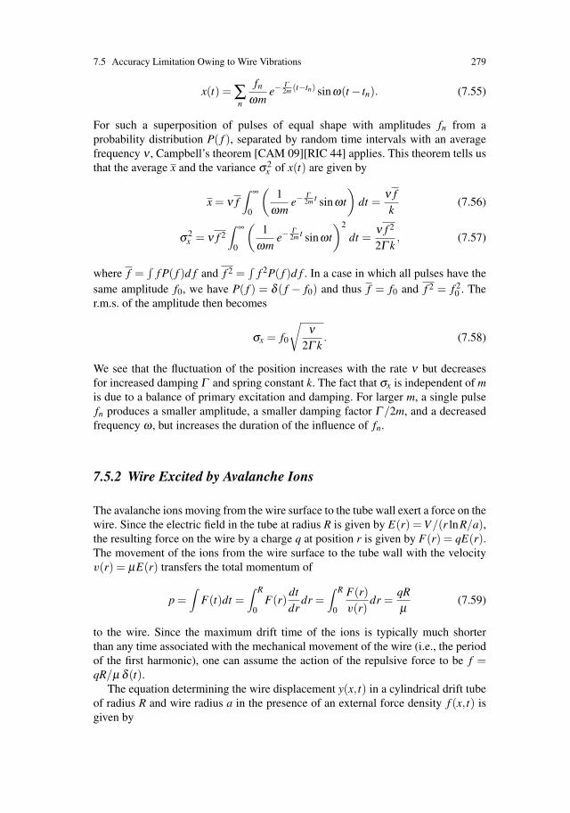
7.5 Accuracy Limitation Owing to Wire Vibrations 279
x(t) = ∑n
fn
ωme−
Γ2m (t−tn) sinω(t − tn). (7.55)
For such a superposition of pulses of equal shape with amplitudes fn from aprobability distribution P( f ), separated by random time intervals with an averagefrequency ν , Campbell’s theorem [CAM 09][RIC 44] applies. This theorem tells usthat the average x and the variance σ2
x of x(t) are given by
x = ν f∫ ∞
0
(1
ωme−
Γ2m t sinωt
)dt =
ν fk
(7.56)
σ2x = ν f 2
∫ ∞
0
(1
ωme−
Γ2m t sinωt
)2
dt =ν f 2
2Γ k, (7.57)
where f =∫
f P( f )d f and f 2 =∫
f 2P( f )d f . In a case in which all pulses have thesame amplitude f0, we have P( f ) = δ ( f − f0) and thus f = f0 and f 2 = f 2
0 . Ther.m.s. of the amplitude then becomes
σx = f0
√ν
2Γ k. (7.58)
We see that the fluctuation of the position increases with the rate ν but decreasesfor increased damping Γ and spring constant k. The fact that σx is independent of mis due to a balance of primary excitation and damping. For larger m, a single pulsefn produces a smaller amplitude, a smaller damping factor Γ /2m, and a decreasedfrequency ω , but increases the duration of the influence of fn.
7.5.2 Wire Excited by Avalanche Ions
The avalanche ions moving from the wire surface to the tube wall exert a force on thewire. Since the electric field in the tube at radius R is given by E(r) = V/(r lnR/a),the resulting force on the wire by a charge q at position r is given by F(r) = qE(r).The movement of the ions from the wire surface to the tube wall with the velocityv(r) = μE(r) transfers the total momentum of
p =∫
F(t)dt =∫ R
0F(r)
dtdr
dr =∫ R
0
F(r)v(r)
dr =qRμ
(7.59)
to the wire. Since the maximum drift time of the ions is typically much shorterthan any time associated with the mechanical movement of the wire (i.e., the periodof the first harmonic), one can assume the action of the repulsive force to be f =qR/μ δ (t).
The equation determining the wire displacement y(x, t) in a cylindrical drift tubeof radius R and wire radius a in the presence of an external force density f (x, t) isgiven by

280 7 Coordinate Measurement and Fundamental Limits of Accuracy
ρ∂ 2y∂ t2 + γ0
∂y∂ t
−T∂ 2y∂x2 −κy = −gρ + f (x, t), (7.60)
where ρ is the linear wire density, γ0 the friction coefficient and T the wire tension.The term κ = 2πε0V 2/(R lnR/a)2 represents the electrostatic force, V is the wirevoltage and gρ the gravitational force. The expression f (x, t) due to the avalanchesof charge qn at time tn, position xn and angular position φn is
f (x, t) =Rμ ∑
nqn cosφn δ (t − tn)δ (x− xn). (7.61)
The solution of Eq. (7.60) and the statistical analysis can be performed in analogyto the simple example from the previous section. The solution obviously dependson the way the excitations are distributed in the azimuthal direction and along thewire, and whether the avalanches are created from a point source or from tracks.Boyko et al. have shown that these different conditions can be collected into onedimensionless constant. They find the resulting variance of the position of the wire,averaged over the wire length, to be given by
σy =qRμ
√ν
12T γ0
√KK1K2, (7.62)
where q is the average total charge per event, ν is the total particle rate on thetube, and K,K1,K2 are dimensionless geometry factors which together make upone constant. This solution assumes that the avalanche ions return to the tube wallalong the trajectories of the primary ionization electrons. For point ionization wehave K = 1 and K1 = 0.5. For particle tracks through the tube we have K = 0.416and K1 = 0.5–1 depending on the angular distribution of the tracks. K2 is anothergeometry factor being ≈ 1 for uniform illumination along the tube.
Figure 7.18 shows results of a calculation assuming a drift tube of R = 1cm,mobility μ = 1.7cm2/Vs and a damping factor γ0 = 7 × 10⁻⁵ kg/sm. The wire
Fig. 7.18 Wire vibrationamplitudes calculated by[BOY 95] for a practical case(see text). The uncertainty ofthe wire position is shown asa function of the count rate.The three bands belong to thethree different avalanche sizesindicated; in each band theupper edge is valid for a wiretension of 50 g and the lowerfor one of 500 g

7.6 Accuracy Limitation Owing to Space Charge Fluctuations 281
tension is varied from 50 to 500 g. The diagram makes it clear that wire vibrationscan be a decisive factor for detectors operating in limited streamer mode (charges of10–100 pC) at fluxes >105 particles/s. In proportional mode (charges around 1 pC)the vibration makes a significant contribution (>10 μm) only in the case of lowerion mobility (larger pressure), lower wire tension, smaller wire damping, and ratesbeyond 1 MHz.
7.6 Accuracy Limitation Owing to Space Charge Fluctuations
There are situations in which the drift time measurement becomes inaccurate owingto fluctuations in the drift field. As an example we discuss the ATLAS MDT drifttubes [ATL 97]. It is expected that their momentum measuring accuracy will bereduced when the photon background rate goes beyond the design level. In thetubes, the background γ-radiation will produce a space charge whose density de-pends on the counting rate, the ion charge per count, the ion drift velocity, andthe tube diameter. The space charge density is homogeneous – which produces afield (increasing linearly from the wire to the tube wall) in addition to the mainfield (proportional to 1/r). This was explained in Sect. 4.5.3 in the context ofthe reduction of amplification. Using the method outlined there, we can estimatethat at a background count rate of 1.4 kHz per cm of wire length (roughly fivetimes the design value), the drift field is distorted to an extent that an apparentshift of track positions of the order of a millimetre takes place in part of the driftspace.
This effect can in principle be corrected by carefully monitoring the history ofthe previous few milliseconds (the ion travel time to the tube wall). If the tube worksperfectly, and if the charge associated with each previous pulse is known, it might bepossible to assess the total ion charge present in the tube at the moment of recordingthe track in question. Then the drift field distortion may be calculated and the trackposition corrected.
However, this procedure is limited by the inhomogeneity of the charge densityalong the tube. Even if there is some knowledge about the average density of countsalong the tube, there is the statistical fluctuation in the immediate vicinity of therecorded track. Before we report a measurement quantifying this effect, let us es-timate what we can expect. At the flux rate of 1400 Hz/cm the charge that willcontribute to the disturbing field is the one produced in roughly 3 cm of tube length(approximately the tube diameter) in 5 ms (the ion travel time to the wall); this cor-responds to 1400Hz/cm× 5ms× 3cm = 21 avalanches on average. As these areoccurring at random we expect a fluctuation of 1/
√21 or 0.22 of the total shift.
Thus if the total shift goes up to the order of 1 mm it will fluctuate on the order of0.2 mm.
In an experiment using a strong radioactive γ-source the ATLAS muon team[ATL 00] irradiated the tubes in the drift chambers, creating background condi-tions five times as severe as expected for the most heavily irradiated parts of the

282 7 Coordinate Measurement and Fundamental Limits of Accuracy
Fig. 7.19 Resolution as afunction of distance from thewire, comparison ofmeasurements andsimulations. Full squares:measurement withoutbackground; open circles:measurement with abackground rate of1400 Hz/cm (4.5 kHz pertube); lines: simulationswithout and with background(36 keV per photon)
spectrometer. The coordinates of high-energy muon tracks were measured at rightangles to the wires, and the resolution was determined. The result of the experimentis shown in Fig. 7.19. The resolution deteriorates enormously in the outer region ofthe tube owing to the presence of the background, and assumes values up to 140 μm.A detailed simulation along the ideas outlined above was carried out and comparedto the measurements. The curves in Fig. 7.19 match the data and show that the effectis understood.
Finally, let us be aware that it is the problem of ageing to which one owes thiscritical dependence of measuring accuracy on background. Had not the hydrocar-bons been outlawed one could find gas mixtures with a much reduced dependenceof the drift velocity on the electric field (cf. the remarks at the end of Sect. 12.6.4).
Appendix to Chapter 7. Influence of Cluster Fluctuationson the Measurement Accuracy of a Single Wire
An analytical form of Eq. (7.15) can be derived under certain assumptions as fol-lows. The symbols used here were defined in Sect. 7.2.
We consider the Nc clusters produced along the track segment R. Nic represents
the clusters of cluster size i, where Nic = NcP(i) and P(i) is the cluster-size distribu-
tion defined in Sect. 1.2.2 [Eq. (1.34)].The Ni
c clusters produce a total of iNic electrons and on average mi of them,
mi = iNcP(i)b
Rcosθ= iNi
cb
Rcosθ, (7.63)
are collected by the wire. The total number N of electrons collected by the wire is

7.6 Accuracy Limitation Owing to Space Charge Fluctuations 283
N = ∑i
mi,
where the sum on i is performed on the cluster size i.As we showed in Sect. 7.2.3, N does not depend on diffusion, and we assume in
the following that neither does each mi.Defining xi to be the average position of the mi electrons collected by the wire
and produced in clusters of original cluster size i, the quantity XAV defined by (7.10)can be rewritten as
XAV = ∑mixi
∑mi= ∑mixi
N. (7.64)
Its variance is given simply by
σ2XAV
= Var(XAV) = ∑m2i Var(xi)N2 , (7.65)
since the various xi are not correlated because they are by definition averages ofarrival positions of electrons produced in different clusters.
The variance of xi, Var (xi), depends on the distribution of the number k(k =0, . . . , i) of collected electrons when i are produced in the same cluster. Referring toEqs. (7.1) and (7.3) and assuming for simplicity x0 = 0, we find that the probabilitythat k electrons among i are collected is given by
1R
+R/2∫
−R/2
ds
⎡⎣
+∞∫−∞
dxG(x|ssinθ ,σx)
⎤⎦
i⎡⎢⎣
+b/2∫
−b/2
dyG(y|scosθ ,σy)
⎤⎥⎦
k
×
⎡⎢⎣1−
+b/2∫
−b/2
dyG(y|scosθ ,σy)
⎤⎥⎦
i−k(i
k
), (7.66)
where the term
(ik
)takes into account the different combinations of k electrons
among i.Since we have assumed that x0 = 0, we also have that
〈x〉 = 〈xi〉 = 〈XAV〉 = 0 . (7.67)
The integrals in dx of (7.66) are equal to 1. Defining
Δ(scosθ) =
+b/2∫
−b/2
dyG(y|scosθ ,σy) (7.68)
as the probability that one electron is collected by the wire (0 < Δ < 1), we rewritethe probability that k among i electrons produced in the same cluster are collected

284 7 Coordinate Measurement and Fundamental Limits of Accuracy
by the wire as
Π ik =
1R
+R/2∫
−R/2
Δ k(1−Δ)i−k
(i
k
)ds . (7.69)
We note that
∑k=0
iΠ ik = 1 .
If along the track segment R we produce Nic clusters of i electrons, on the wire we
collect on average
• NicΠ i
1 single electrons• Ni
cΠ i2 pairs of electrons
• NicΠ i
3 triplets of electrons• . . .• Ni
cΠ ii ith of electrons
and in total we have
Nic
i
∑k=0
kΠ iK = mi
electrons. This last equality can be proved using (7.69) and (7.68) and the propertiesof the binomial distribution.
The number Nipairs of different pairs of electrons produced in the same cluster of
cluster size i and collected by the wire is given by
Nipairs = Ni
c
i
∑k=2
(k
2
)Π i
k =Ni
c
2
(i
∑k=0
k2Π ik −
i
∑k=0
kΠ ik
)
=Ni
c
2
i
∑k=0
k2Π ik −
mi
2. (7.70)
We are now in a position to compute the variance Var (xi) of the average positionxi of the mi electrons produced by clusters of cluster size i and collected by the wire:we have mi variance terms 〈x2〉 and 2×Ni
pairs covariance terms 〈xx〉. The average〈xi〉 is zero because we have assumed that x0 = 0 in (7.66) [see also (7.67)]. Weobtain
Var(xi) =mi〈x2〉+Ni
pairs〈xx〉m2
i
=mi〈x2〉+
(Ni
c ∑ik=0 k2Π i
k −mi)〈xx〉
m2i
=1mi
[(〈x2〉−〈xx〉)+
∑ik=0 k2Π i
k
∑ik=0 kΠ i
k
〈xx〉]
. (7.71)

7.6 Accuracy Limitation Owing to Space Charge Fluctuations 285
Using (7.69) and the properties of the binomial distribution, one can show that
i
∑k=0
k2Π ik =
i2 − iR
+R/2∫
−R/2
Δ 2ds+iR
+R/2∫
−R/2
Δds ,
i
∑k=0
kΠ ik =
iR
+R/2∫
−R/2
Δ 2ds .
From these equations we obtain
∑ik=0 k2Π i
k
∑ik=0 kΠ i
k
= 1+(i−1)I2 ,
where
I2 =
+R/2∫−R/2
Δ 2ds
+R/2∫−R/2
Δds
, (7.72)
and we can rewrite (7.71) as
Var(xi) =1mi
(〈x2〉− I2〈xx〉+ iI2〈xx〉) . (7.73)
Finally we substitute the variance Var(xi) from this last equation into (7.65) andset
Var(XAV) = ∑mi(〈x2〉− I2〈xx〉+ iI2〈xx〉)N2
=〈x2〉− I2〈xx〉
N+ ∑ imi
N2 I2〈xx〉 . (7.74)
Using (7.63) we can show that
∑i imi
N2 = ∑i i2NcP(i)[b/(Rcosθ)]N2 = ∑i i2NcP(i)[b/(Rcosθ)]
(∑i iNcP(i)[b/(Rcosθ)])2
=∑ j n2
j(∑ j n j
)2
1b/(Rcosθ)
=1
Neff, (7.75)
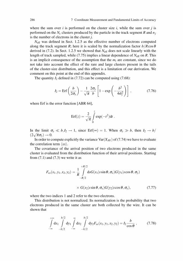
286 7 Coordinate Measurement and Fundamental Limits of Accuracy
where the sum over i is performed on the cluster size i, while the sum over j isperformed on the Nc clusters produced by the particle in the track segment R and n j
is the number of electrons in the cluster j.Neff was defined in Sect. 1.2.5 as the effective number of electrons computed
along the track segment R; here it is scaled by the normalization factor b/Rcosθderived in (7.2). In Sect. 1.2.5 we showed that Neff does not scale linearly with thelength of track sampled, while (7.75) implies a linear dependence of Neff on R. Thisis an implicit consequence of the assumption that the mi are constant, since we donot take into account the effect of the rare and large clusters present in the tailsof the cluster-size distribution, and this effect is a limitation of our derivation. Wecomment on this point at the end of this appendix.
The quantity I2 defined in (7.72) can be computed using (7.68):
I2 = Erf
(b
2σy
)− 1√
π2σy
b
[1− exp
(− b2
4σ2y
)], (7.76)
where Erf is the error function [ABR 64],
Erf(z) =2√π
z∫0
exp(−t2)dt .
In the limit σy b, I2 → 1, since Erf(∞) = 1. When σy � b, then I2 → b/(2√
πσy) → 0.In order to compute explicitly the variance Var(XAV) of (7.74) we have to evaluate
the correlation term 〈xx〉.The covariance of the arrival position of two electrons produced in the same
cluster is evaluated from the distribution function of their arrival positions. Startingfrom (7.1) and (7.3) we write it as
Fxx(x1,y1,x2,y2) =1R
+R/2∫
−R/2
dsG(x1|ssinθ ,σx)G(y1|scosθ ,σy)
× G(x2|ssinθ ,σx)G(y2|scosθ ,σy), (7.77)
where the two indices 1 and 2 refer to the two electrons.This distribution is not normalized. Its normalization is the probability that two
electrons produced in the same cluster are both collected by the wire. It can beshown that
+∞∫−∞
dx1
b/2∫
−b/2
dy1
∞∫−∞
dx2
b/2∫
−b/2
dy2Fxx(x1,y1,x2,y2) = I2b
cosθ, (7.78)

7.6 Accuracy Limitation Owing to Space Charge Fluctuations 287
where I2 is defined by (7.72). Since in (7.74) we have the product I2〈xx〉, we cancompute directly
I2〈xx〉 =cosθ
b
+∞∫−∞
dx1
b/2∫
−b/2
dy1
×+∞∫
−∞
dx2
+b/2∫
−b/2
dy2x1x2Fxx(x1,y1,x2,y2) , (7.79)
and after some tedious integration we obtain
I2〈xx〉 = tan2 θ
[(σ2
y +b2
12
)(Erf
(b
2σy
)− 2√
πσy
b
(1− exp
[− b2
4σ2y
]))
+ b2 13√
π
(4
σ3y
b3
(1− exp
[− b2
4σ2y
])− σy
b
)
− σ2y
1√π
(σy
b
(1− exp
[− b2
4σ2y
]))]. (7.80)
Now we have all the information we require and can write down the final formulafor the variance Var(XAV). Using (7.74), (7.75), (7.5) and (7.80) yields
σ2XAV
= Var(XAV) = σ2x
1N
+ tan2 θσ2y
[1N
+(
1Neff
− 1N
)Fσ
(σy
b
)]
+ tan2 θb2
12
[1N
+(
1Neff
− 1N
)Fb
(σy
b
)], (7.81)
where the two functions Fσ and Fb are given by
Fσ = Erf
(b
2σy
)− 3√
πσy
b
(1− exp
[− b2
4σ2y
])(7.82)
Fb = Erf
(b
2σy
)− 2√
πσy
b
(1− exp
[− b2
4σ2y
])(1−8
σ2y
b2
)− 4√
πσy
b. (7.83)
These are equal to 1 when σy/b is zero and go to zero when σy/b → ∞. Inspecting(7.81) we note that this behaviour corresponds to a smooth transition between thecoefficients 1/Neff and 1/N in the angular terms. In the absence of diffusion there iscomplete correlation and the reduction factor of the angular term in the variance of

288 7 Coordinate Measurement and Fundamental Limits of Accuracy
Fig. 7.20 Declustering as afunction of σ/b. Plot of thefunctions defined in (7.82)and (7.83)
the average (7.10) is only Neff; when the diffusion is large compared to the width bof the drift cell, there is no correlation and the reduction factor of the angular termis N, the total number of collected electrons. The functions Fσ and Fb are shown inFig. 7.20.
If we had calculated the plot of Fig. 7.3 with (7.81) (instead of using the numer-ical simulation (see Sect. 7.2.3)), we would have found a similar behaviour but asomewhat steeper increase of Neff(σ) with σ/l. This is a consequence of the as-sumption introduced: we have assumed that the average number mi of electronsoriginated by clusters of size i and collected by the wire is constant. If we do notmake this assumption, then (7.65) contains an additional term,
Var(XAV) = ∑m2i Var(xi)N2 + ∑(xi −XAV)2Var(mi)
N2 . (7.84)
The second term plays a role when the rare large clusters are present, since theydominate the average. The numerical simulation introduced in Sect. 7.2.3 and usedto produce Fig. 7.3 takes into account all the various effects due to the peculiarshape of the cluster-size distribution and then correctly produces a variance largerthan that evaluated in (7.81) and consequently a smaller Neff(σ).
References
[ABR 64] M. Abramovitz and I. Stegun (eds.), Handbook of Mathematical Functions (Dover,New York 1964) p. 297.
[AME 83] S.R. Amendolia et al. E×B and angular effects in the avalanche localization along thewire with cathode pad readout, Nucl. Instrum. Methods 217, 317 (1983)
[ATL 00] M. Aleksa, M. Deile, J. Dubbert, C.W. Fabjan, C. Gruhn, N.P. Hessey, W. Riegler andT. Sammer, Rate effects in high-resolution drift chambers, Nucl. Instr. Meth. Phys.
References 289
Res. A 435-443 (2000), also M. Aleksa, Doctoral Diss. Performance of the ATLASMuon Spectrometer, Techn. Univ. Wien (Sept. 1999)
[ATL 97] ATLAS Muon spectrometer: Technical Design Report, CERN, Geneva, Switzerland,CERN/LHC 97-22, 1997
[BAR 82] A. Barbaro Galtieri, Tracking with the PEP-4 TPC, TPC-LBL 82-24, Berkeley preprint1982 (unpublished)
[BLU 86] W. Blum, U. Stiegler, P. Gondolo and L. Rolandi, Measurement of the avalanchebroadening caused by the wire E×B effect, Nucl. Instrum. Methods A 252, 407 (1986)
[BOY 95] I. R. Boyko, G. A. Chelkov, V. I. Dodonov, M. A. Ignatenko, M. Yu. Nikolenko, Vi-bration of signal wires in wire detectors under irradiation, Nucl. Instrum. Methods inPhys. Res. A367, 321 (1995)
[CAM 09] N. R. Campbell, The study of discontinuous phenomena, Proc. Cambridge Phys. Soc.,15, 117–136 (1909)
[CRA 51] H. Cramer, Mathematical Methods of Statistics (Princeton Univ. Press 1951), Sec. 28.6[HAR 84] C.K. Hargrove et al., The spatial resolution of the time projection chamber at TRIUMF,
Nucl. Instrum. Methods 219, 461 (1984)[RIC 44] S.O. Rice, Mathematical Analysis of Random Noise, Bell Syst. techn. J. 23, 282
(1994), 24, 46 (1945), reprinted in: N. Wax, Selected Papers on Noise and Stochas-tic Processes, (Dover Publications, New York 1954, 2003)
446


Chapter 8Geometrical Track Parameters and Their Errors
Now we come to the point to which all the efforts of drift-chamber design lead up –the determination of the track parameters. The point of origin of a track, its angles oforientation, and its curvature in a magnetic field are the main geometric propertiesthat one aims to measure. The proof of the pudding is in the eating, and the proof ofthe drift chamber is in the track parameters.
In a particle experiment a track is often measured by several detectors, and theaccuracy of its parameters depends on the integrity of the whole ensemble, and inparticular on the knowledge of the relative detector positions. Likewise, the trackparameters determined with a drift chamber depend on its overall geometry, theelectrode positions, fields and electron drift paths. If one wants to calculate theachievable accuracy of a drift chamber in all parts of its volume, one needs tohave quantitative knowledge of these factors in addition to the point-measuring ac-curacy. Such knowledge is often difficult to get, and then one may want to workthe other way around: starting from a measurement of the achieved accuracy oftrack parameters, one can compare it to that expected from the point-measuringaccuracy alone. If they agree, then the other factors make only a small contri-bution, if they do not, the contribution of the other factors is larger, or perhapsdominant.
The achieved accuracy can be measured in a number of ways. The common meth-ods include the following: vertex localization by comparing tracks from the samevertex, momentum resolution by measuring tracks with known momentum, a com-bination of momentum and angular precision with a measurement of the invariantmass of a decaying particle.
It is obviously our first task to ascertain the accuracy that can be achieved in agiven geometry when considering the resolution of each measuring point alone, ig-noring all the other factors by assuming they are negligible or have been correctedfor. We will do this in two sections, one for the situation without magnetic field,using straight-line fits, the other for the situation inside a magnetic field, where aquadratic fit is appropriate. One section is devoted to accuracy limitations due tomultiple Coulomb scattering in parts of the apparatus. Finally, the results on spec-trometer resolution are summarized.
W. Blum et al., Particle Detection with Drift Chambers, 291doi: 10.1007/978-3-540-76684-1 8, c© Springer-Verlag Berlin Heidelberg 2008
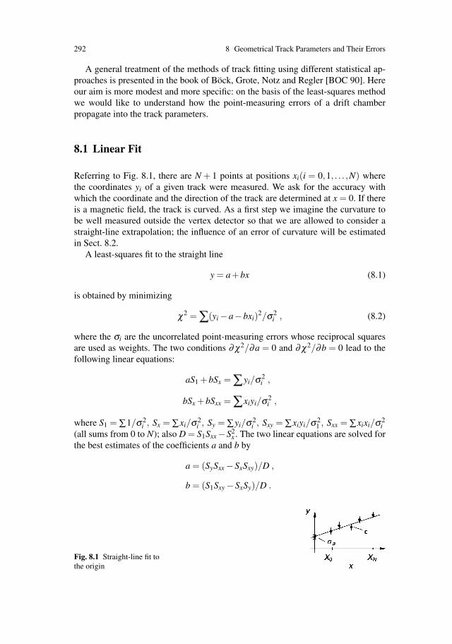
292 8 Geometrical Track Parameters and Their Errors
A general treatment of the methods of track fitting using different statistical ap-proaches is presented in the book of Bock, Grote, Notz and Regler [BOC 90]. Hereour aim is more modest and more specific: on the basis of the least-squares methodwe would like to understand how the point-measuring errors of a drift chamberpropagate into the track parameters.
8.1 Linear Fit
Referring to Fig. 8.1, there are N + 1 points at positions xi(i = 0,1, . . . ,N) wherethe coordinates yi of a given track were measured. We ask for the accuracy withwhich the coordinate and the direction of the track are determined at x = 0. If thereis a magnetic field, the track is curved. As a first step we imagine the curvature tobe well measured outside the vertex detector so that we are allowed to consider astraight-line extrapolation; the influence of an error of curvature will be estimatedin Sect. 8.2.
A least-squares fit to the straight line
y = a+bx (8.1)
is obtained by minimizing
χ2 = ∑(yi −a−bxi)2/σ2i , (8.2)
where the σi are the uncorrelated point-measuring errors whose reciprocal squaresare used as weights. The two conditions ∂ χ2/∂a = 0 and ∂ χ2/∂b = 0 lead to thefollowing linear equations:
aS1 +bSx = ∑yi/σ2i ,
bSx +bSxx = ∑xiyi/σ2i ,
where S1 = ∑1/σ2i , Sx = ∑xi/σ2
i , Sy = ∑yi/σ2i , Sxy = ∑xiyi/σ2
1 , Sxx = ∑xixi/σ2i
(all sums from 0 to N); also D = S1Sxx −S2x . The two linear equations are solved for
the best estimates of the coefficients a and b by
a = (SySxx −SxSxy)/D ,
b = (S1Sxy −SxSy)/D .
Fig. 8.1 Straight-line fit tothe origin
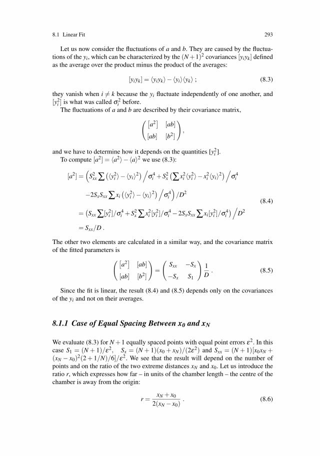
8.1 Linear Fit 293
Let us now consider the fluctuations of a and b. They are caused by the fluctua-tions of the yi, which can be characterized by the (N +1)2 covariances [yiyk] definedas the average over the product minus the product of the averages:
[yiyk] = 〈yiyk〉−〈yi〉〈yk〉 ; (8.3)
they vanish when i �= k because the yi fluctuate independently of one another, and[y2
i ] is what was called σ2i before.
The fluctuations of a and b are described by their covariance matrix,([
a2]
[ab]
[ab] [b2]
),
and we have to determine how it depends on the quantities [y2i ].
To compute [a2] = 〈a2〉−〈a〉2 we use (8.3):
[a2] =(
S2xx ∑
(〈y2
i 〉−〈yi〉2)/σ4i +S2
x
(∑x2
i 〈y2i 〉− x2
i 〈yi〉2)/σ4i
−2SxSxx ∑xi(〈y2
i 〉−〈yi〉2)/σ4i
)/D2
=(Sxx ∑[y2
i ]/σ4i +S2
x ∑x2i [y
2i ]/σ4
i −2SxSxx ∑xi[y2i ]/σ4
i
)/D2
= Sxx/D .
(8.4)
The other two elements are calculated in a similar way, and the covariance matrixof the fitted parameters is
([a2]
[ab]
[ab] [b2]
)=
(Sxx −Sx
−Sx S1
)1D
. (8.5)
Since the fit is linear, the result (8.4) and (8.5) depends only on the covariancesof the yi and not on their averages.
8.1.1 Case of Equal Spacing Between x0 and xN
We evaluate (8.3) for N +1 equally spaced points with equal point errors ε2. In thiscase S1 = (N + 1)/ε2, Sx = (N + 1)(x0 + xN)/(2ε2) and Sxx = (N + 1)[x0xN +(xN − x0)2(2 + 1/N)/6]/ε2. We see that the result will depend on the number ofpoints and on the ratio of the two extreme distances xN and x0. Let us introduce theratio r, which expresses how far – in units of the chamber length – the centre of thechamber is away from the origin:
r =xN + x0
2(xN − x0). (8.6)
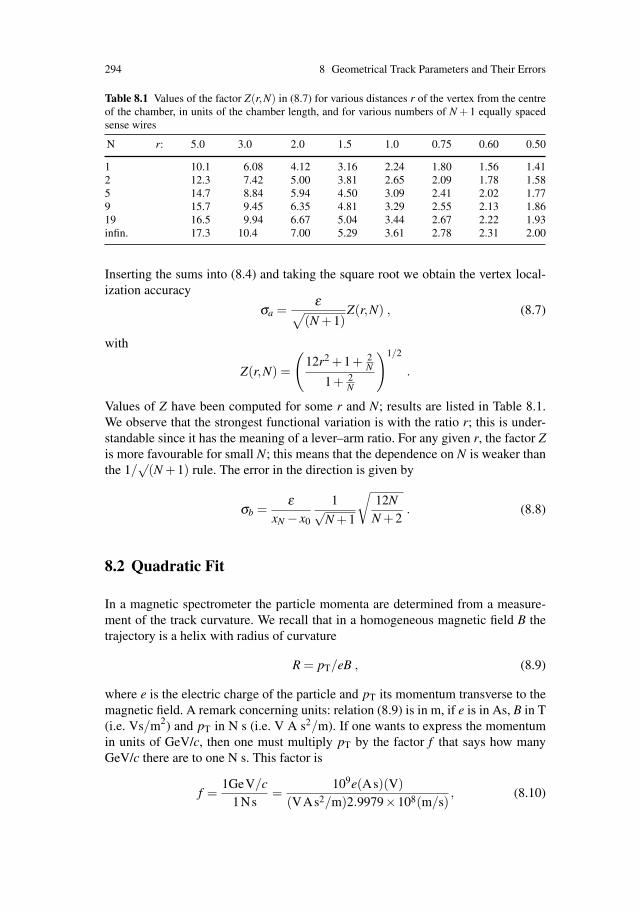
294 8 Geometrical Track Parameters and Their Errors
Table 8.1 Values of the factor Z(r,N) in (8.7) for various distances r of the vertex from the centreof the chamber, in units of the chamber length, and for various numbers of N + 1 equally spacedsense wires
N r: 5.0 3.0 2.0 1.5 1.0 0.75 0.60 0.50
1 10.1 6.08 4.12 3.16 2.24 1.80 1.56 1.412 12.3 7.42 5.00 3.81 2.65 2.09 1.78 1.585 14.7 8.84 5.94 4.50 3.09 2.41 2.02 1.779 15.7 9.45 6.35 4.81 3.29 2.55 2.13 1.8619 16.5 9.94 6.67 5.04 3.44 2.67 2.22 1.93infin. 17.3 10.4 7.00 5.29 3.61 2.78 2.31 2.00
Inserting the sums into (8.4) and taking the square root we obtain the vertex local-ization accuracy
σa =ε√
(N +1)Z(r,N) , (8.7)
with
Z(r,N) =
(12r2 +1+ 2
N
1+ 2N
)1/2
.
Values of Z have been computed for some r and N; results are listed in Table 8.1.We observe that the strongest functional variation is with the ratio r; this is under-standable since it has the meaning of a lever–arm ratio. For any given r, the factor Zis more favourable for small N; this means that the dependence on N is weaker thanthe 1/
√(N +1) rule. The error in the direction is given by
σb =ε
xN − x0
1√N +1
√12N
N +2. (8.8)
8.2 Quadratic Fit
In a magnetic spectrometer the particle momenta are determined from a measure-ment of the track curvature. We recall that in a homogeneous magnetic field B thetrajectory is a helix with radius of curvature
R = pT/eB , (8.9)
where e is the electric charge of the particle and pT its momentum transverse to themagnetic field. A remark concerning units: relation (8.9) is in m, if e is in As, B in T(i.e. Vs/m2) and pT in N s (i.e. V A s2/m). If one wants to express the momentumin units of GeV/c, then one must multiply pT by the factor f that says how manyGeV/c there are to one N s. This factor is
f =1GeV/c
1Ns=
109e(As)(V)(VAs2/m)2.9979×108(m/s)
, (8.10)

8.2 Quadratic Fit 295
so that (8.9), to better than one tenth of a percent, takes on the simple form
R =103
(Tm
GeV/c
)pT
B. (8.11)
This radius has to be measured in a plane perpendicular to B. Our interest is in thelarge momenta because they are the most difficult to measure precisely. Thereforewe approximate the helix trajectory, which is actually a circle in a plane perpendic-ular to its axis, by a parabola in such a plane,
y = a+bx+(c/2)x2 , (8.12)
up to terms of the order of x3/R2, where c = 1/R. The measured yi at positions xi
are fitted to (8.12) with the aim of determining a, b and c.
8.2.1 Error Calculation
One is interested in the errors of a, b and c. Our procedure is similar to that ofGluckstern [GLU 63], but is more general in that it includes the extrapolation to avertex point at an arbitrary distance.
The linear equations for a, b and c are derived from the conditions of a minimalχ2 and read as follows (the weighting factor at each point is denoted by fn):
aF0 +bF1 +(c/2)F2 = ∑ fnyn ,
aF1 +bF2 +(c/2)F3 = ∑ fnxnyn (8.13)
aF2 +bF3 +(c/2)F4 = ∑ fnx2nyn ,
whereFj = ∑ fn(xn) j . (8.14)
All sums run from n = 0 to n = N. The solution of (8.13) for our three quantities is
a = ∑ynGn
∑Gn,
b = ∑ynPn
∑xnPn, (8.15)
c2
= ∑ynQn
∑x2nQn
,
where the Gn, Pn and Qn are expressed using determinants of the Fj:
Gn = fn
∣∣∣∣F2 F3
F3 F4
∣∣∣∣− fnxn
∣∣∣∣F1 F2
F3 F4
∣∣∣∣+ fnx2n
∣∣∣∣F1 F2
F2 F3
∣∣∣∣ ,

296 8 Geometrical Track Parameters and Their Errors
Pn = − fn
∣∣∣∣F1 F3
F2 F4
∣∣∣∣+ fnxn
∣∣∣∣F0 F2
F2 F4
∣∣∣∣− fnx2n
∣∣∣∣F0 F1
F2 F3
∣∣∣∣ ,
Qn = fn
∣∣∣∣F1 F2
F2 F3
∣∣∣∣− fnxn
∣∣∣∣F0 F1
F2 F3
∣∣∣∣+ fnx2n
∣∣∣∣F0 F1
F1 F2
∣∣∣∣ .
They have the property that
∑Qn = ∑xnQn = ∑Pn
= ∑x2nPn = ∑xnGn = ∑x2
nGn = 0 (8.16)
and
∑x2nQn = ∑xnPn = ∑Gn . (8.17)
Using (8.16), the variance of the first coefficient is given by
[a2] = ∑∑GmGn[ymyn]/(
∑Gn)2
, (8.18)
where [ymyn] denotes the covariance of the measurements at two points xm and xn.The other elements are formed in the same manner.
The point-measurement errors are equal and uncorrelated. We write
[yn ym] = ε2δmm (8.19)
and obtain[a2]= ε2 ∑G2
n
/(∑Gn
)2,
[ab] = ε2 ∑GnPn
/(∑Gn
)(∑xnPn
),
[b2]= ε2 ∑P2
n
/(∑xnPn
)2, (8.20)
[ac] = 2ε2 ∑GnQn
/(∑Gn
)(∑x2
nQn)
,
[bc] = ε22∑QnPn
/(∑x2
nQn)(
∑xnPn)
,
[c2]= ε24∑Q2
n
/(∑x2
nQn)2
.
8.2.2 Origin at the Centre of the Track – Uniform Spacing of Wires
In order to facilitate the evaluation of (8.20) we begin by setting the origin of the xcoordinates at the centre of the track. Let

8.2 Quadratic Fit 297
qn = xn − xc, with xc = ∑xn/(N +1) , (8.21)
andL = xN − x0 .
For uniform spacing and uniform weights fn = 1, the subdeterminants are easilycalculated to be
Gn = F2F4 −q2nF2
2 ,
Pn = qn(F0F4 −F22 ) ,
Qn = −F22 +q2
nF0F2 ,
with Fj = ∑q j. Note that F1 = F3 = 0 for symmetry. The other Fj are
F0 = N +1 ,
F2 = L2 (N +1)(N +2)12N
,
F4 = L4 (N +1)(N +2)(3N2 +6N −4)240N3 ,
S = F0F4 −F22 = L4 (N −1)(N +1)2(N +2)(N +3)
180N3 ,
(8.22)
A combination S, needed later, has been included here. Inserting the subdetermi-nants into (8.20) we find the six elements of the covariance matrix, valid at theorigin, that is the centre of the track:
[a2]= ε2F4/(F0F4 −F2
2 ) ,
[ab] = 0 ,
[b2]= ε2/F2 ,
[ac] = −2ε2F2/(F0F4 −F22 ) ,
[bc] = 0 ,
[c2]= 4F0/(F0F4 −F2
2 ) .
(8.23)
Note that there is no correlation between the direction b and the offset a or thecurvature c in the middle of the track. The elements of the covariance matrix (8.23)will assume different values outside the centre, and this will be treated in Sect. 8.2.4.The variance of the curvature, however, is the same all along the track, and we canevaluate it by inserting (8.22) into the last of the equations (8.23). The variance of

298 8 Geometrical Track Parameters and Their Errors
Table 8.2 Values of the factors AN in (8.24) and √(AN)/8 in (8.26) for various values of N. (Thenumber of measuring points is N +1.)
N AN√(AN)/8
2 96 1.223 81 1.124 73.1 1.075 67.0 1.026 61.7 0.9828 53.2 0.91210 46.6 0.853
infin.720
N +53.35√N +5
the curvature is equal to
[c2] =ε2
L4
720N3
(N −1)(N +1)(N +2)(N +3)=
ε2
L4 AN , (8.24)
where we have defined a factor AN , some values of which are enumerated inTable 8.2.
8.2.3 Sagitta
The maximum excursion of a piece of a circle over the corresponding chord is calledits sagitta. The sagitta s of a track with length L and radius of curvature R � Lis proportional to the square of the track length, as can be seen from the sketchof Fig. 8.2 when developing the cosine of the small angle (L/2R) into powers of(L/2R):
s = L2/8R , (8.25)
so its r.m.s. error becomes
δ s = ε√
AN
8. (8.26)
This ratio between the errors of the sagitta and the individual point coordinates isalso contained in Table 8.2.
Fig. 8.2 Sagitta s
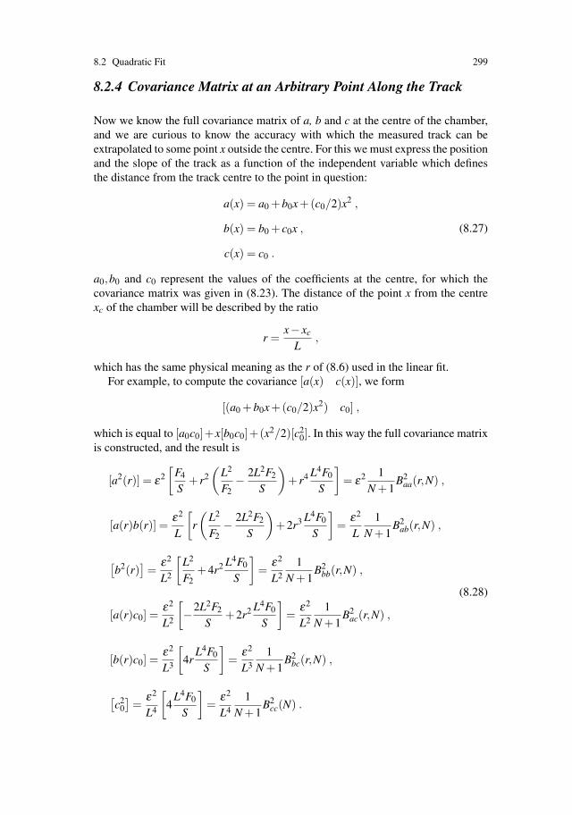
8.2 Quadratic Fit 299
8.2.4 Covariance Matrix at an Arbitrary Point Along the Track
Now we know the full covariance matrix of a, b and c at the centre of the chamber,and we are curious to know the accuracy with which the measured track can beextrapolated to some point x outside the centre. For this we must express the positionand the slope of the track as a function of the independent variable which definesthe distance from the track centre to the point in question:
a(x) = a0 +b0x+(c0/2)x2 ,
b(x) = b0 + c0x ,
c(x) = c0 .
(8.27)
a0,b0 and c0 represent the values of the coefficients at the centre, for which thecovariance matrix was given in (8.23). The distance of the point x from the centrexc of the chamber will be described by the ratio
r =x− xc
L,
which has the same physical meaning as the r of (8.6) used in the linear fit.For example, to compute the covariance [a(x) c(x)], we form
[(a0 +b0x+(c0/2)x2) c0] ,
which is equal to [a0c0]+x[b0c0]+(x2/2)[c20]. In this way the full covariance matrix
is constructed, and the result is
[a2(r)] = ε2[
F4
S+ r2
(L2
F2− 2L2F2
S
)+ r4 L4F0
S
]= ε2 1
N +1B2
aa(r,N) ,
[a(r)b(r)] =ε2
L
[r
(L2
F2− 2L2F2
S
)+2r3 L4F0
S
]=
ε2
L1
N +1B2
ab(r,N) ,
[b2(r)
]=
ε2
L2
[L2
F2+4r2 L4F0
S
]=
ε2
L2
1N +1
B2bb(r,N) ,
[a(r)c0] =ε2
L2
[−2L2F2
S+2r2 L4F0
S
]=
ε2
L2
1N +1
B2ac(r,N) ,
[b(r)c0] =ε2
L3
[4r
L4F0
S
]=
ε2
L3
1N +1
B2bc(r,N) ,
[c2
0
]=
ε2
L4
[4
L4F0
S
]=
ε2
L4
1N +1
B2cc(N) .
(8.28)
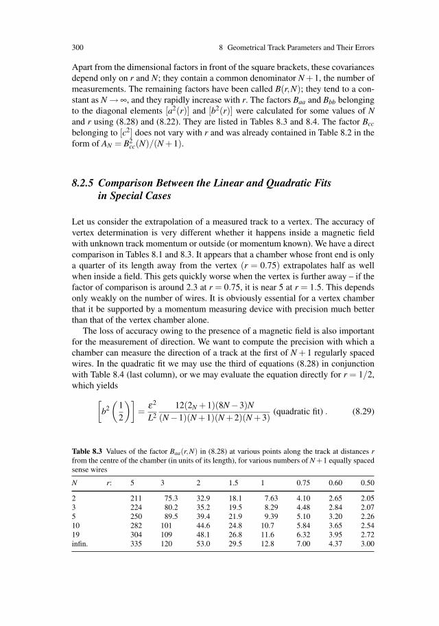
300 8 Geometrical Track Parameters and Their Errors
Apart from the dimensional factors in front of the square brackets, these covariancesdepend only on r and N; they contain a common denominator N +1, the number ofmeasurements. The remaining factors have been called B(r,N); they tend to a con-stant as N → ∞, and they rapidly increase with r. The factors Baa and Bbb belongingto the diagonal elements [a2(r)] and [b2(r)] were calculated for some values of Nand r using (8.28) and (8.22). They are listed in Tables 8.3 and 8.4. The factor Bcc
belonging to [c2] does not vary with r and was already contained in Table 8.2 in theform of AN = B2
cc(N)/(N +1).
8.2.5 Comparison Between the Linear and Quadratic Fitsin Special Cases
Let us consider the extrapolation of a measured track to a vertex. The accuracy ofvertex determination is very different whether it happens inside a magnetic fieldwith unknown track momentum or outside (or momentum known). We have a directcomparison in Tables 8.1 and 8.3. It appears that a chamber whose front end is onlya quarter of its length away from the vertex (r = 0.75) extrapolates half as wellwhen inside a field. This gets quickly worse when the vertex is further away – if thefactor of comparison is around 2.3 at r = 0.75, it is near 5 at r = 1.5. This dependsonly weakly on the number of wires. It is obviously essential for a vertex chamberthat it be supported by a momentum measuring device with precision much betterthan that of the vertex chamber alone.
The loss of accuracy owing to the presence of a magnetic field is also importantfor the measurement of direction. We want to compute the precision with which achamber can measure the direction of a track at the first of N + 1 regularly spacedwires. In the quadratic fit we may use the third of equations (8.28) in conjunctionwith Table 8.4 (last column), or we may evaluate the equation directly for r = 1/2,which yields
[b2(
12
)]=
ε2
L2
12(2N +1)(8N −3)N(N −1)(N +1)(N +2)(N +3)
(quadratic fit) . (8.29)
Table 8.3 Values of the factor Baa(r,N) in (8.28) at various points along the track at distances rfrom the centre of the chamber (in units of its length), for various numbers of N +1 equally spacedsense wires
N r: 5 3 2 1.5 1 0.75 0.60 0.50
2 211 75.3 32.9 18.1 7.63 4.10 2.65 2.053 224 80.2 35.2 19.5 8.29 4.48 2.84 2.075 250 89.5 39.4 21.9 9.39 5.10 3.20 2.2610 282 101 44.6 24.8 10.7 5.84 3.65 2.5419 304 109 48.1 26.8 11.6 6.32 3.95 2.72infin. 335 120 53.0 29.5 12.8 7.00 4.37 3.00
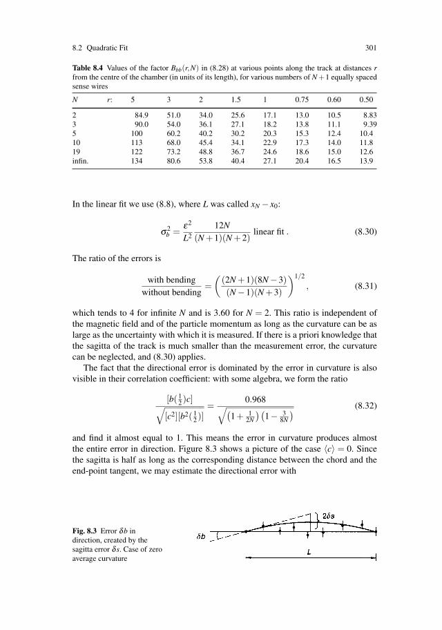
8.2 Quadratic Fit 301
Table 8.4 Values of the factor Bbb(r,N) in (8.28) at various points along the track at distances rfrom the centre of the chamber (in units of its length), for various numbers of N +1 equally spacedsense wires
N r: 5 3 2 1.5 1 0.75 0.60 0.50
2 84.9 51.0 34.0 25.6 17.1 13.0 10.5 8.833 90.0 54.0 36.1 27.1 18.2 13.8 11.1 9.395 100 60.2 40.2 30.2 20.3 15.3 12.4 10.410 113 68.0 45.4 34.1 22.9 17.3 14.0 11.819 122 73.2 48.8 36.7 24.6 18.6 15.0 12.6infin. 134 80.6 53.8 40.4 27.1 20.4 16.5 13.9
In the linear fit we use (8.8), where L was called xN − x0:
σ2b =
ε2
L2
12N(N +1)(N +2)
linear fit . (8.30)
The ratio of the errors is
with bendingwithout bending
=(
(2N +1)(8N −3)(N −1)(N +3)
)1/2
, (8.31)
which tends to 4 for infinite N and is 3.60 for N = 2. This ratio is independent ofthe magnetic field and of the particle momentum as long as the curvature can be aslarge as the uncertainty with which it is measured. If there is a priori knowledge thatthe sagitta of the track is much smaller than the measurement error, the curvaturecan be neglected, and (8.30) applies.
The fact that the directional error is dominated by the error in curvature is alsovisible in their correlation coefficient: with some algebra, we form the ratio
[b( 12 )c]√
[c2][b2( 12 )]
=0.968√(
1+ 12N
)(1− 3
8N
) (8.32)
and find it almost equal to 1. This means the error in curvature produces almostthe entire error in direction. Figure 8.3 shows a picture of the case 〈c〉 = 0. Sincethe sagitta is half as long as the corresponding distance between the chord and theend-point tangent, we may estimate the directional error with
Fig. 8.3 Error δb indirection, created by thesagitta error δ s. Case of zeroaverage curvature

302 8 Geometrical Track Parameters and Their Errors
δb =2δ sL/2
. (8.33)
Using (8.26),(8.24) and (8.29) one may verify that (8.33) is correct within 4% forall N.
8.2.6 Optimal Spacing of Wires
With a given number N + 1 of wires and a given chamber length L the elements ofthe covariance matrix can be minimized by varying the wire positions. SummarizingGluckstern [GLU 63] we mention that the optimal spacing is different for differentcorrelation coefficients, and that for a minimal [c2] the best wire positions are ideallythe following:
(N +1)/4 wires at x = 0, (N +1)/2 wires at x = L/2 ,
(N +1)/4 wires at x = L .
In practice the clustering of wires will use some of the chamber length. For the idealcase this was set to zero, and he calculates at r = −1/2 that[
b2
(12
)]= ε2
L272
N+1 ,
[b
(12
)c
]= − ε2
L3128
N+1 ,
[c2]= ε2
L4256
N+1 ,
(8.34)
and this, at large N, is an important factor of 1.7 better in the momentum resolutionthan (8.28).
8.3 A Chamber and One Additional MeasuringPoint Outside
It happens quite often that tracks are measured not only in the main drift chamberbut in addition at some extra point which is located some distance away from themain chamber. Typical examples are a miniature vertex detector near the beam pipe,or a single layer of chambers surrounding the central main chamber. In an event withtracks coming from the same vertex, the vertex constraint serves a similar purpose,especially when the vertex position must be the same for many events. We supposethat all the measurements happen inside a magnetic field.
Since we have developed the covariance matrix of the variables a, b and c at anarbitrary point r along the track, we have the tools to add the constraint of the oneadditional space-coordinate measurement. The scheme to do this is the following.

8.3 A Chamber and One Additional Measuring Point Outside 303
Let the full covariance matrix at r (8.28) be abbreviated by
Cik(r) =
⎛⎜⎜⎜⎝
[a2(r)
][a(r)b(r)] [a(r)c]
[a(r)b(r)][b2(r)
][b(r)c]
[a(r)c] [b(r)c][c2]
⎞⎟⎟⎟⎠ . (8.35)
This matrix has to be inverted to obtain the χ2 matrix C−1ik (r). The corresponding
matrix D−1ik of the additional measuring point has only the one element that belongs
to the space-coordinate non-zero; let us call it 1/ε2v (εv is the accuracy of the addi-
tional measuring point):
D−1ik =
⎛⎝ ε−2
v 0 0
0 0 00 0 0
⎞⎠ . (8.36)
Now the covariance matrix Eik of the total measurement, N + 1 regularly spacedwires plus this one point, a distance rL away from their centre, is given by theinverse of the sum of the inverses of the individual covariances:
(Eik)−1 = (Cik(r))−1 +(Dik)−1 (8.37)
Now there is a theorem (e.g. [SEL 72]) which states that if the inverse of a firstmatrix is known, then the inverse of a second matrix, which differs from the first inonly one element, can be calculated according to a simple formula. In our case thefirst matrix is C−1, and its known inverse is C; the second matrix, E−1, differs fromthe first only in the (1, 1) element which is larger by 1/ε2
v . The inverse of the secondmatrix is given by
Eik = Cik −C1iC1k
ε2v +C11
. (8.38)
This means that our covariance matrix (8.28) changes by the addition of one pointat r according to the following scheme (we leave out the argument r):
[a2]→ [a′2] = [a2]− [a2]2
ε2v +[a2]
,
[ab] → [a′b′] = [ab]− [a2][ab]ε2
v +[a2],
[b2]→ [b′2] = [b2]− [ab2]2
ε2v +[a2]
,
[ac] → [a′c′] = [ac]− [a2][ac]ε2
v +[a2],
[bc] → [b′c′] = [bc]− [ab][ac]ε2
v +[a2],
[c2]→ [c′2] = [c2]− [ac]2
ε2v +[a2]
.
(8.39)
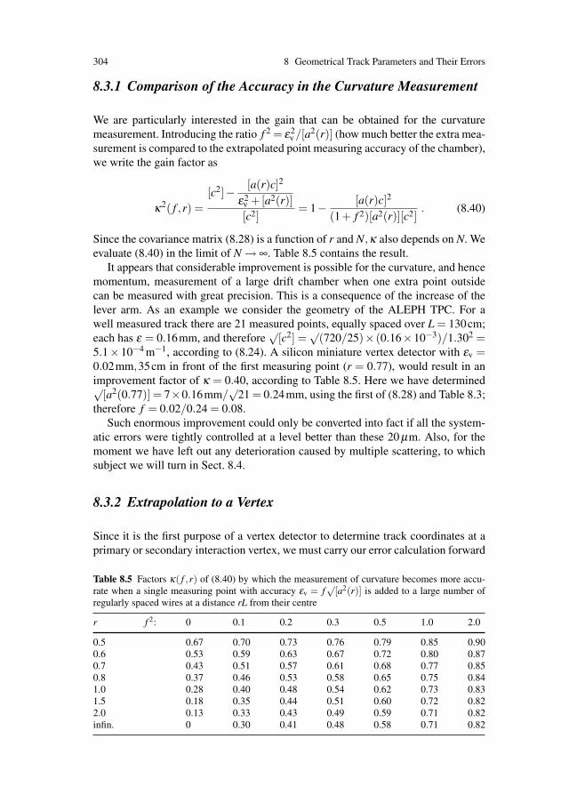
304 8 Geometrical Track Parameters and Their Errors
8.3.1 Comparison of the Accuracy in the Curvature Measurement
We are particularly interested in the gain that can be obtained for the curvaturemeasurement. Introducing the ratio f 2 = ε2
v /[a2(r)] (how much better the extra mea-surement is compared to the extrapolated point measuring accuracy of the chamber),we write the gain factor as
κ2( f ,r) =[c2]− [a(r)c]2
ε2v +[a2(r)][c2]
= 1− [a(r)c]2
(1+ f 2)[a2(r)][c2]. (8.40)
Since the covariance matrix (8.28) is a function of r and N,κ also depends on N. Weevaluate (8.40) in the limit of N → ∞. Table 8.5 contains the result.
It appears that considerable improvement is possible for the curvature, and hencemomentum, measurement of a large drift chamber when one extra point outsidecan be measured with great precision. This is a consequence of the increase of thelever arm. As an example we consider the geometry of the ALEPH TPC. For awell measured track there are 21 measured points, equally spaced over L = 130cm;each has ε = 0.16mm, and therefore
√[c2] =
√(720/25)× (0.16×10−3)/1.302 =
5.1× 10⁻⁴ m−1, according to (8.24). A silicon miniature vertex detector with εv =0.02mm,35cm in front of the first measuring point (r = 0.77), would result in animprovement factor of κ = 0.40, according to Table 8.5. Here we have determined√
[a2(0.77)] = 7×0.16mm/√
21 = 0.24mm, using the first of (8.28) and Table 8.3;therefore f = 0.02/0.24 = 0.08.
Such enormous improvement could only be converted into fact if all the system-atic errors were tightly controlled at a level better than these 20 μm. Also, for themoment we have left out any deterioration caused by multiple scattering, to whichsubject we will turn in Sect. 8.4.
8.3.2 Extrapolation to a Vertex
Since it is the first purpose of a vertex detector to determine track coordinates at aprimary or secondary interaction vertex, we must carry our error calculation forward
Table 8.5 Factors κ( f ,r) of (8.40) by which the measurement of curvature becomes more accu-rate when a single measuring point with accuracy εv = f
√[a2(r)] is added to a large number of
regularly spaced wires at a distance rL from their centre
r f 2: 0 0.1 0.2 0.3 0.5 1.0 2.0
0.5 0.67 0.70 0.73 0.76 0.79 0.85 0.900.6 0.53 0.59 0.63 0.67 0.72 0.80 0.870.7 0.43 0.51 0.57 0.61 0.68 0.77 0.850.8 0.37 0.46 0.53 0.58 0.65 0.75 0.841.0 0.28 0.40 0.48 0.54 0.62 0.73 0.831.5 0.18 0.35 0.44 0.51 0.60 0.72 0.822.0 0.13 0.33 0.43 0.49 0.59 0.71 0.82infin. 0 0.30 0.41 0.48 0.58 0.71 0.82

8.3 A Chamber and One Additional Measuring Point Outside 305
Fig. 8.4 Extrapolation of thequadratic fit to a vertexlocated a distance x in front ofa vertex detector withaccuracy ±εv. The N +1wires of a chamber areuniformly spaced over thelength L. The vertex detectoris a distance xv away from thecentre of the wires. In thetext, r = xv/L
to the vertex. The situation is sketched in Fig. 8.4. The coordinate x represents thedistance of the detector to the vertex, and the extrapolation error Δ of the vertexposition is given by the covariance
Δ 2 = [y2] = [(a′(r)+b′(r)x+ c′(r)x2/2)2]
= [a′2]+2x[a′b′]+ x2([b′2]+ [a′c′])
+ x3[b′c′]+ x4[c′2]/4 .
(8.41)
Here the [a′2], [a′b′], . . . represent the elements of the covariance matrix E (8.39) atthe position r of the vertex detector.
The evaluation of (8.41) is too clumsy when done in full generality, and we willconsider the special case of a vertex detector that is much more accurate than thedrift chamber at r, as presented in Table 8.3:
f 2 1
orε2
v [a2(r)] . (8.42)
The covariance matrix at r for the ensemble of chamber and vertex detector, in firstorder of ε2
v /[a2(r)], takes the form
E =
⎛⎜⎜⎝
ε2v ε2
v [ab]/[a2] ε2v [ac]/[a2]
ε2v [ab]/[a2] [b2]− [ab]2/[a2] [bc]− [ab][ac]/[a2]
ε2v [ac]/[a2] [bc]− [ab][ac]/[a2] [c2]− [ac]2/[a2]
⎞⎟⎟⎠ . (8.43)
The elements of E depend on N and r. We evaluate (8.43) in the limit of N → ∞ andfor some special values of r. For r = 1/2 (i.e. the vertex detector at the same placeas the last wire), using (8.41), (8.42), (8.28), (8.22), one finds that
Δ 2 =ε2
N +1
(48
x2
L2 +120x3
L3 +80x4
L4
)+ ε2
v
(1+8.0
xL
+6.7x2
L2
).

306 8 Geometrical Track Parameters and Their Errors
Fig. 8.5a,b Graph of the twofunctions in (8.44) for fourpositions r of the vertexdetector; (a) R(r,x/L), (b)S(r,x/L)
Here we have counted x/L positive if x and xv point in the same direction. We seethat the vertex extrapolation accuracy deteriorates as x/L increases. There is oneterm proportional to the accuracy squared of the vertex detector alone, and one termproportional to the quantity ε2/(N +1), which characterizes the accuracy of the driftchamber.
Δ 2 = R2(
r,xL
) ε2
N +1+S2
(r,
xL
)ε2
v . (8.44)
Figure 8.5a,b contains graphs of R(r,x/L) and S(r,x/L) for four values of r in therange of typical applications.
Taking again the geometry of the ALEPH experiment as a numerical example,we read from Fig. 8.5a,b that for r = 0.77 and xv = 6.5cm the vertex extrapolationaccuracy can reach Δ =
√(0.282ε2/21 + 1.142ε2
v ). Using ε = 160μm and εv =20μm one obtains Δ = 25μm in this particular case.
8.4 Limitations Due to Multiple Scattering
The achievable accuracy of a chamber may be reduced by multiple scattering of themeasured particle in some piece of the apparatus. There it suffers a displacementand a change in direction, and we want to know the influence on the accuracy ofvertex reconstruction and of momentum measurement.
8.4.1 Basic Formulae
The theory of multiple scattering has been developed by Moliere, Snyder, Scott,Bethe and others. Reviews exist from Rossi [ROS 52], Bethe [BET 53] and Scott[SCO 63]. Our interest here must be limited to the basic notions.
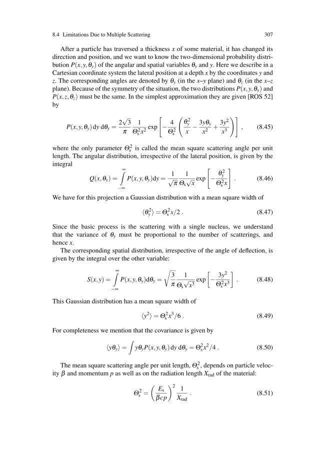
8.4 Limitations Due to Multiple Scattering 307
After a particle has traversed a thickness x of some material, it has changed itsdirection and position, and we want to know the two-dimensional probability distri-bution P(x,y,θy) of the angular and spatial variables θy and y. Here we describe in aCartesian coordinate system the lateral position at a depth x by the coordinates y andz. The corresponding angles are denoted by θy (in the x–y plane) and θz (in the x–zplane). Because of the symmetry of the situation, the two distributions P(x,y,θy) andP(x,z,θz) must be the same. In the simplest approximation they are given [ROS 52]by
P(x,y,θy)dy dθy =2√
3π
1Θ 2
s x2 exp
[− 4
Θ 2s
(θ 2
y
x− 3yθy
x2 +3y2
x3
)], (8.45)
where the only parameter Θ 2s is called the mean square scattering angle per unit
length. The angular distribution, irrespective of the lateral position, is given by theintegral
Q(x,θy) =∞∫
−∞
P(x,y,θy)dy =1√π
1Θs
√x
exp
[−
θ 2y
Θ 2s x
]. (8.46)
We have for this projection a Gaussian distribution with a mean square width of
〈θ 2y 〉 = Θ 2
s x/2 . (8.47)
Since the basic process is the scattering with a single nucleus, we understandthat the variance of θy must be proportional to the number of scatterings, andhence x.
The corresponding spatial distribution, irrespective of the angle of deflection, isgiven by the integral over the other variable:
S(x,y) =∞∫
−∞
P(x,y,θy)dθy =
√3π
1
Θs
√x3
exp
[− 3y2
Θ 2s x3
]. (8.48)
This Gaussian distribution has a mean square width of
〈y2〉 = Θ 2s x3/6 . (8.49)
For completeness we mention that the covariance is given by
〈yθy〉 =∫
yθyP(x,y,θy)dy dθy = Θ2s x2/4 . (8.50)
The mean square scattering angle per unit length, Θ 2s , depends on particle veloc-
ity β and momentum p as well as on the radiation length Xrad of the material:
Θ 2s =
(Es
βcp
)2 1Xrad
. (8.51)
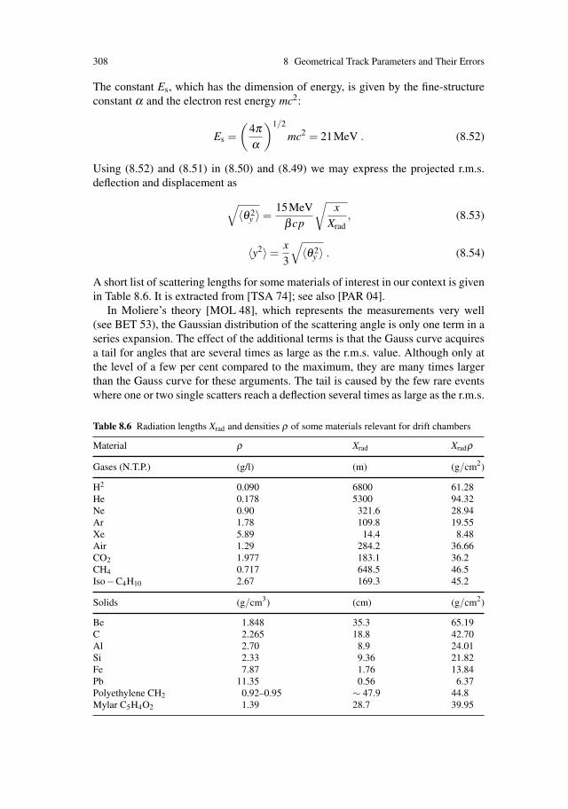
308 8 Geometrical Track Parameters and Their Errors
The constant Es, which has the dimension of energy, is given by the fine-structureconstant α and the electron rest energy mc2:
Es =(
4πα
)1/2
mc2 = 21MeV . (8.52)
Using (8.52) and (8.51) in (8.50) and (8.49) we may express the projected r.m.s.deflection and displacement as
√〈θ 2
y 〉 =15MeV
βcp
√x
Xrad, (8.53)
〈y2〉 =x3
√〈θ 2
y 〉 . (8.54)
A short list of scattering lengths for some materials of interest in our context is givenin Table 8.6. It is extracted from [TSA 74]; see also [PAR 04].
In Moliere’s theory [MOL 48], which represents the measurements very well(see BET 53), the Gaussian distribution of the scattering angle is only one term in aseries expansion. The effect of the additional terms is that the Gauss curve acquiresa tail for angles that are several times as large as the r.m.s. value. Although only atthe level of a few per cent compared to the maximum, they are many times largerthan the Gauss curve for these arguments. The tail is caused by the few rare eventswhere one or two single scatters reach a deflection several times as large as the r.m.s.
Table 8.6 Radiation lengths Xrad and densities ρ of some materials relevant for drift chambers
Material ρ Xrad Xradρ
Gases (N.T.P.) (g/l) (m) (g/cm2)
H2 0.090 6800 61.28He 0.178 5300 94.32Ne 0.90 321.6 28.94Ar 1.78 109.8 19.55Xe 5.89 14.4 8.48Air 1.29 284.2 36.66CO2 1.977 183.1 36.2CH4 0.717 648.5 46.5Iso−C4H10 2.67 169.3 45.2
Solids (g/cm3) (cm) (g/cm2)
Be 1.848 35.3 65.19C 2.265 18.8 42.70Al 2.70 8.9 24.01Si 2.33 9.36 21.82Fe 7.87 1.76 13.84Pb 11.35 0.56 6.37Polyethylene CH2 0.92–0.95 ∼ 47.9 44.8Mylar C5H4O2 1.39 28.7 39.95

8.4 Limitations Due to Multiple Scattering 309
sum of the large majority of events, which are dominated by small-angle scatteringalone. This behaviour is typical for Coulomb scattering as described by the Ruther-ford formula; for hadrons, nuclear elastic scattering also makes a contribution to thetail. All the theories that go beyond the simple approximation discussed above areanalytically quite complex.
Highland [HIG 75] has taken a practical standpoint by fitting the width of thescattering-angle distribution of the Moliere theory to a form similar to (8.53), usingthe radiation lengths as listed in the Particle Data Tables (and partly in our Table 8.6).
He finds that the width of Moliere does not vary appreciably with the nuclearcharge number Z; he introduces an x-dependent correction factor (1 + ε(x)) to(8.53), which redefines the energy constant. His result is
θ 1/ey =
14.1MeVβcp
√x
Xrad
(1+
19
log10x
Xrad
). (8.55)
θ 1/ey is the angle in the x–y plane at which the Moliere probability density is down
by a factor of 1/e from the maximum. Formula (8.55) is supposed to be accurate to5% in the range 10−3 < x/Xrad < 10, except for the very light elements, where theaccuracy is 10–20%.
8.4.2 Vertex Determination
At colliders the observation of primary vertices and of secondary vertices from par-ticles with short lifetimes is through a vacuum tube; in addition there is the materialof the vertex chamber itself. We would like to compute the vertex localization errordue to multiple scattering in these materials. The situation is sketched in Fig. 8.6.We assume for simplicity that the track is infinitely well measured outside the scat-tering material. Upon extrapolation, it misses the vertex position by the distance d.The average over the square of d is equal to
〈d2〉 = 〈ϑ 21 〉r2
1 + 〈ϑ 22 〉r2
2 + · · · , (8.56)
where the mean squared projected scattering angle 〈ϑ 21 〉 is given by the thickness ti
of the layer i in units of radiation lengths of the material i according to (8.53), where〈ϑ 2〉 = 〈θ 2
y 〉. We express the r.m.s. value of d in terms of a ‘Coulomb scattering
Fig. 8.6 Coulomb multiplescattering of an infinitely wellmeasured track

310 8 Geometrical Track Parameters and Their Errors
limit’ Sc of the vertex localization accuracy. By combining (8.56) and (8.53) wehave √
〈d2〉 =Sc
β pc, (8.57)
withSc = 15MeV
(∑ tir
2i
)1/2. (8.58)
Practical values of Sc range between 45 and 200μm GeV for various experiments;compare Table 11.3.
The above calculation gives correct vertex errors in the limit that the Coulombscattering is much larger than the measurement errors and that all the scattering ma-terial is between the sense wires and the vertex. For the general case the estimationof vertex errors is more involved. Although the quadratic addition of measure-ment errors (8.7) and the multiple-scattering errors (8.57) gives the right order ofmagnitude for the total, more sophisticated estimation methods give better results.Lutz [LUT 88] has developed an optimal tracking procedure by fitting the individualcontributions to multiple scattering between the measuring points.
8.4.3 Resolution of Curvature for Tracks Througha Scattering Medium
We have seen in (8.53) that the mean square scattering angle increases as themomentum of the particle becomes smaller. Let us imagine a drift chamber in aspectrometer where the momentum of a particle is low enough to make the multiple-scattering error the dominating one. We would like to know the accuracy for ameasurement of the curvature in this situation; this implies we suppose that the ac-curacy of the apparatus itself is infinitely better than the multiple-scattering errors.
We resume the arguments of Sect. 8.2 at (8.2.1). In order to evaluate [ynym] in thecase of multiple scattering, we observe that
[ynym] = [yn(yn +(xm − xn)θyn] = [y2n]+ (xm − xn)[ynθyn] (8.59)
for xm ≥ xn. Now we make use of (8.49) and (8.50) and obtain
[ynym] = Θ 2s x2
n(3xm − xn)/12 . (8.60)
Gluckstern [GLU 63] has evaluated the correlation coefficients at the first ofN +1 uniformly spaced wires with the result
[c2]MS =Θ 2
s
2LCN ,
[cb
(12
)]MS
= −Θ 2s
2DN , (8.61)
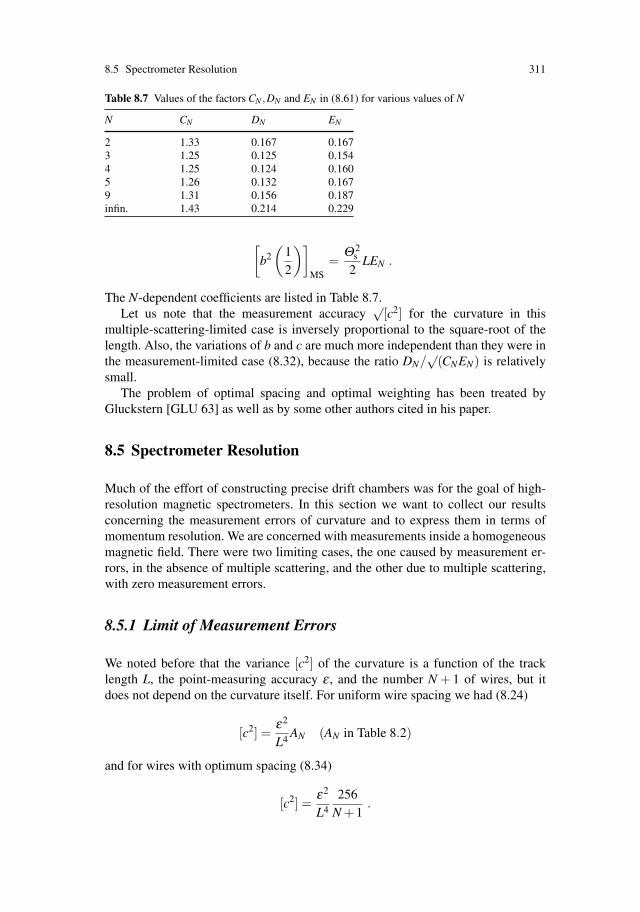
8.5 Spectrometer Resolution 311
Table 8.7 Values of the factors CN ,DN and EN in (8.61) for various values of N
N CN DN EN
2 1.33 0.167 0.1673 1.25 0.125 0.1544 1.25 0.124 0.1605 1.26 0.132 0.1679 1.31 0.156 0.187infin. 1.43 0.214 0.229
[b2(
12
)]MS
=Θ 2
s
2LEN .
The N-dependent coefficients are listed in Table 8.7.Let us note that the measurement accuracy
√[c2] for the curvature in this
multiple-scattering-limited case is inversely proportional to the square-root of thelength. Also, the variations of b and c are much more independent than they were inthe measurement-limited case (8.32), because the ratio DN/
√(CNEN) is relatively
small.The problem of optimal spacing and optimal weighting has been treated by
Gluckstern [GLU 63] as well as by some other authors cited in his paper.
8.5 Spectrometer Resolution
Much of the effort of constructing precise drift chambers was for the goal of high-resolution magnetic spectrometers. In this section we want to collect our resultsconcerning the measurement errors of curvature and to express them in terms ofmomentum resolution. We are concerned with measurements inside a homogeneousmagnetic field. There were two limiting cases, the one caused by measurement er-rors, in the absence of multiple scattering, and the other due to multiple scattering,with zero measurement errors.
8.5.1 Limit of Measurement Errors
We noted before that the variance [c2] of the curvature is a function of the tracklength L, the point-measuring accuracy ε , and the number N + 1 of wires, but itdoes not depend on the curvature itself. For uniform wire spacing we had (8.24)
[c2] =ε2
L4 AN (AN in Table 8.2)
and for wires with optimum spacing (8.34)
[c2] =ε2
L4
256N +1
.
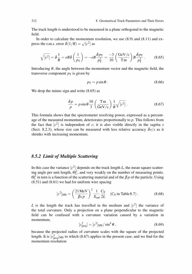
312 8 Geometrical Track Parameters and Their Errors
The track length is understood to be measured in a plane orthogonal to the magneticfield.
In order to calculate the momentum resolution, we use (8.9) and (8.11) and ex-press the r.m.s. error δ (1/R) =
√[c2] as
√[c2] = δ
1R
= eBδ(
1pT
)= −eB
δ pT
p2T
=−310
(GeV/c
Tm
)B
δ pT
p2T
. (8.65)
Introducing θ , the angle between the momentum vector and the magnetic field, thetransverse component pT is given by
pT = psinθ . (8.66)
We drop the minus sign and write (8.65) as
δ pp
= psinθ103
(Tm
GeV/c
)1B
√[c2] . (8.67)
This formula shows that the spectrometer resolving power, expressed as a percent-age of the measured momentum, deteriorates proportionally to p. This follows fromthe fact that [c2] is independent of c; it is also visible directly in the sagitta s(Sect. 8.2.3), whose size can be measured with less relative accuracy δ s/s as itshrinks with increasing momentum.
8.5.2 Limit of Multiple Scattering
In this case the variance [c2] depends on the track length L, the mean square scatter-ing angle per unit length, Θ 2
s , and very weakly on the number of measuring points.Θ 2
s in turn is a function of the scattering material and of the β p of the particle. Using(8.51) and (8.61) we had for uniform wire spacing
[c2]MS =(
21MeVβcp
)2 1Xrad
CN
2L(CN in Table8.7) . (8.68)
L is the length the track has travelled in the medium and [c2] the variance ofthe total curvature. Only a projection on a plane perpendicular to the magneticfield can be confused with a curvature variation caused by a variation inmomentum,
[c2proj] = [c2]MS/sin4 θ , (8.69)
because the projected radius of curvature scales with the square of the projectedlength. It is [c2
proj]MS to which (8.67) applies in the present case, and we find for themomentum resolution

References 313
δ pp
=p
sinθ103
(Tm
GeV/c
)1B
√[c2]MS .
=21(MeV/c)
β sinθ103
(Tm
GeV/c
)1B
√CN
2LXrad.
(8.70)
We see that the multiple-scattering limit of the momentum resolution is inde-pendent of momentum because, as p goes up, the decrease in bending power iscompensated by the decrease in the scattering angle. According to (8.70), a muontraversing 1 m of magnetized iron (2T) at right angles to the field cannot be mea-sured better than to 22%, even if there were infinitely many measuring points withinfinite accuracy inside the iron. Depending on the apparatus, L will often be a func-tion of the angle θ .
References
[BET 53] H.A. Bethe, Moliere’s theory of multiple scattering, Phys. Rev. 89, 1256 (1953)[BOC 90] R.K. Bock, H. Grote, D. Notz, M. Regler, Data analysis techniques for high-energy
physics experiments (Cambridge University Press, Cambridge, UK 1990)[GLU 63] R.L. Gluckstern, Uncertainties in track momentum and direction due to multiple scat-
tering and measurement errors, Nucl. Instr. Meth. 24, 381 (1963)[HIG 75] V.L. Highland, Some practical remarks on multiple scattering, Nucl. Instrum. Meth-
ods 129, 497 (1975)[LUT 88] G. Lutz, Optimum track fitting in the presence of multiple scattering, Nucl. Instrum.
Methods Phys. Res. A 273, 349 (1988)[MOL 48] G. Moliere, Theorie der Streuung schneller geladener Teilchen II, Mehrfach und
Vielfachstreuung, Z. Naturforsch. 3a, 78 (1948)[PAR 04] Particle Data Group, Review of Particle Properties, Phys. Lett. B 592 (2004)[ROS 52] B. Rossi, High-Energy Particles (Prentice-Hall, Englewood Cliffs, NJ, USA 1952)[SCO 63] W.T. Scott, The theory of small-angle multiple scattering of fast charged particles,
Rev. Mod. Phys. 35, 231 (1963)[SEL 72] S.M. Selby (ed.), Standard Mathematical Tables (The Chemical Rubber Co.,
Cleveland, Ohio, USA 1972)[TSA 74] Y.-S. Tsai, Pair production and bremsstrahlung of charged leptons, Rev. Mod. Phys.
46, 815 (1974)

Chapter 9Ion Gates
Here we wish to take up the subject of ion shutters, which are sometimes placedin the drift space in order to block the passage of electrons or ions. In Chap. 3 weintroduced such wire grids in the context of the electrostatics of drift chambers,stressing the relation between the various grids and electrodes that make up a driftchamber. So far we have dealt with the most straightforward type of gating grid,where all the wires are at the same potential.
For applications in large drift chambers there are more sophisticated forms of ionshutters which, in some modes of operation, have different transmission propertiesfor electrons and for heavy ions.
We will begin this chapter by inspecting the conditions that make it necessary toinvolve gating grids (Sect. 9.1). Then we will survey various forms of gating gridsthat are in use in particle experiments (Sect. 9.2). Finally we compute values forthe transparency under various conditions for which we make use of the results ofChap. 2 concerning ion drift velocities and the magnetic drift properties of electronsin gases.
9.1 Reasons for the Use of Ion Gates
9.1.1 Electric Charge in the Drift Region
Any free charges in the drift volume give rise to electric fields which superim-pose themselves on the drift field and distort it. Chambers with long drift lengthsL are particularly delicate, especially when they are operated with a low drift field.The displacement σx of an electron drift path at its arrival point is of the orderof the drift length times the ratio of the disturbing field Edist over the drift fieldEdrift:
σx = LEdist
Edrift. (9.1)
W. Blum et al., Particle Detection with Drift Chambers, 315doi: 10.1007/978-3-540-76684-1 9, c© Springer-Verlag Berlin Heidelberg 2008

316 9 Ion Gates
This holds if the disturbing field is orthogonal to the drift field, thus causing adisplacement of the field lines to the side, but it also holds if the disturbing fieldacts in the same direction as the drift field, thus causing a change in the velocity andhence of the arrival time, provided the chamber works in the unsaturated mode ofthe drift velocity (cf. Chap. 12).
Free charges can originate as electrons or gas ions from the ionization in thedrift volume, travelling in opposite directions according to their proper drift veloc-ities, or they can be ions from the wire avalanches that have found their way intothe drift region, where they move towards the negative high-voltage electrode. Thislast category contributes the largest part because for every incoming electron whichcauses G avalanche ions to be produced at the proportional wire, there will be Gεin the drift space, where ε is the fraction that arrives in the drift space rather thanon the cathodes opposite the proportional wire. If there is no gating grid, Gε willbe of the order of 103 in typical conditions, but could also be larger (see remarksbelow).
In order to estimate the size of disturbing fields we consider two examples. Thefirst is a drift chamber in which a gas discharge burns continuously between somesense wires and their cathodes. Such a self-sustained process could be caused bysome surface deposit on the cathode, or otherwise. Let the total current be 1μA, andlet ε = 5% of it penetrate into the drift volume. If the ion drift velocity there is 2 m/s,then the linear charge density in the column of travelling ions is λ = 25× 10−9 As/m. Using Gauss’ theorem in this cylindrical geometry, the resulting radial field adistance r away amounts to
Edist =λ
2πrε0= 450(V )
1r
. (9.2)
Here we have neglected the presence of any conductors.The second example is the ALEPH TPC, irradiated by some ionizing radiation,
say cosmic rays or background radiation from the e+e− collider. Let the rate densityof electrons liberated in the sensitive volume be R(s−1m−3). For every electron, Gεions will appear in the drift space, where they travel with velocity vD. Therefore thetotal charge density in the volume has the value.
ρ =eRLGε
vD, (9.3)
where e is the charge of the electron and L is the length of the drift volume. ρ coulddepend on the radius r, as one would expect from radiation originating along thebeam. Let the TPC be approximated by the space between two infinite coaxial con-ducting cylinders with radii r1 = 0.3 m and r2 = 2 m, with the drift direction parallelto the common axis. The cylinders are grounded. The radial field Er is calculatedfrom Maxwell’s equations,
∇Er =1r
∂∂ r
rEr =ρε0
, (9.4)

9.1 Reasons for the Use of Ion Gates 317
r2∫r1
Erdr = 0 .
If ρ(r) = ρ0 does not depend on r, as in the case of irradiation by cosmic rays, theresulting radial disturbing field takes the form
Er(r) =ρ0
2ε0
(r− 1
2rr2
2 − r21
ln(r2/r1)
). (9.5)
If we insert into (9.3) values that are characteristic for the ALEPH TPC irradiatedby cosmic rays at sea level (R = 2×10⁶ s−1m−3, vD = 1.5 m/s, Gε = 103,L = 2 m),we find that ρ0 = 0.43×10⁻⁹ A s m−3. Figure 9.1 shows the radial field that resultsfrom (9.5) in this particular example. We notice that it is negative close to the innerfield cage and positive close to the outer one. Compared to the regular axial driftfield of 104 V/m, it amounts to a fraction of a per cent.
It should be mentioned that the coefficient ε is not very well known. A lower limitcan be evaluated assuming that the amplification produced ions uniformly aroundthe proportional wire. In this case ε is equal to the fraction of electric field lines thatreach from the sense wire into the drift region. Using the formalism of Sect. 3.2 εis equal to the ratio of the surface charge densities on the high-voltage plane and onthe sense wire grid:
ε =|σp|σs
, (9.6)
typically between 3 and 5%.However, it is known that the amplification is not isotropic around the propor-
tional wire. This has been discussed in Sect. 4.3. Large avalanches tend to go aroundthe wire; small avalanches develop on the side where the electrons have arrived. Theions from the small avalanches may go into the drift space more efficiently. Nothingquantitative has been published concerning this question.
Fig. 9.1 Radial dependenceof the electric field producedby a uniform chargedistribution in a cylindricalTPC. The scales are from theexample discussed in the text

318 9 Ion Gates
Some further uncertainty exists concerning the value of vD. The effect of chargetransfer between the travelling ions and any gas molecules of low ionization poten-tial will substitute these molecules, which are often much slower, for the originalions; see Table 2.2. This effect creates a space charge that is not uniform in the driftdirection.
The most important contribution to space charge is usually created by the back-ground radiation at the accelerator. Background conditions can be very differentfrom one experiment to the other. In the ALEPH TPC at LEP (sensitive volume45m3) the sense-wire current is ∼ 0.5μA under standard operating conditions. TheUA1 central detector at the CERN SppS (sensitive volume 25m3) had a current of∼ 120μA at the peak luminosity of 3×1029 cm−2 s−1 [BEI 88].
9.1.2 Ageing
There is experimental evidence of a deterioration in performance of drift and pro-portional chambers after they have been used for some time. Once the total chargecollected on the anode wires during their lifetime exceeds some value between 10−4
and 1 C per cm of wire length, a loss of gain and excessive dark currents are observedin many chambers. Whereas a short account of this problem is given in Sect. 12.6,we mention it in the context of ion gates in order to underline their effect on theageing process.
The dose mentioned above is the product of the incoming charge and the gainfactor. The limit of observable deteriorations depend very much on the gas com-position and on the electric field on the electrode surfaces; under carefully chosenconditions, a limiting dose of the order of 0.1 to 1 C/cm should be achievable. Somemodern experiments even expect to achieve 10 C/cm (cf. Sect. 12.6). The ageingprocess can be stretched in time if only part of the radiation is admitted to the sensewires, using a gate that is triggered only on interesting events.
9.2 Survey of Field Configurations and Trigger Modes
In order to describe the various forms of gating grids employed in particle ex-periments we use two classifications, one according to drift paths on the basis ofdifferent (electric and magnetic) field configurations, the other according to the dy-namical behaviour, i.e. how the gates are switched in connection with events in time.
9.2.1 Three Field Configurations
The simplest gate is the one which has all its wires at the same potential (monopolargating grid). We have stated in Sect. 3.3 that it is closed to incoming electrons andoutgoing ions if all the field lines terminate on it, provided the common potential islarge enough and positive (Fig. 3.10b).

9.2 Survey of Field Configurations and Trigger Modes 319
There is a technical difficulty connected with this configuration: any transitionfrom the closed to the open state must occur in a time interval ΔT comparable tothe electron travel time over a distance small compared to the sensitive drift length,say ΔT ≈ 1μs or less. The charge brought onto the grid in this short time causes anenormous disturbance on the nearby sense wires, orders of magnitudes larger than asignal. One solution to this problem is the introduction of a ‘shielding grid’ betweenthe gating grid and the anode [BRY 85].
Another way to circumvent this difficulty is to close the gating grid byramping two opposite potentials +ΔVg and −ΔVg on neighbouring wires [BRE 80,NEM 83]. In this case the net amount of charge on the gating grid does notchange, and in a first approximation there is no charge induced in the other elec-trodes of the drift chamber. This type of grid is called a bipolar gating grid.In the closed state it has positive charge on every second wire and negativecharge on the wires in between; the drift field lines terminate on the positivecharges.
In the presence of a magnetic field B the drift paths of electrons are no longerthe electric field lines, because their drift-velocity vector has components along Band along [E ×B] according to (2.6). The exact behaviour is governed by the pa-rameter ωτ , or the ion mobility multiplied by the magnitude of the B field. Thisparameter is always very small for ions in drift chambers but can be much largerthan one for electrons in suitable gases (cf. Chap. 2). If this is the case and ΔVg
is increased from zero, the ions are stopped first, while many of the electrons arestill able to penetrate. The reason is the reduced electron mobility towards the gat-ing grid wires. As ΔVg is further increased, the gate is finally closed also for theelectrons.
This bipolar gating grid in a magnetic field, with a suitable value of ΔVg,can therefore be operated as a diode ([AME 85-1] and later but independently[KEN 84]). The electrons from the drift region make their way through the grid ontrajectories which are bent in the wire direction as well as in the direction orthogo-nal to both the wires and the main drift direction. See Fig. 9.2 for an illustration ofthe principle.
Fig. 9.2 Scheme of thebipolar grid immersed in amagnetic field, which makesit transparent to electronswhile it remains opaque toions
320 9 Ion Gates
9.2.2 Three Trigger Modes
The simplest case is the bipolar gating grid operated in a magnetic field as a diode. Itdoes not have to be triggered, and one avoids all switching circuitry and all pick-upproblems. There is a disadvantage to this solution: although the positive ions fromthe wire avalanches are not admitted back into the drift space, all the electrons fromthe drift region are allowed to produce avalanches. Under conditions where chamberageing is a problem, one gives away a factor of the lifetime of the chamber whichdepends on the background conditions of the experiment.
The tightest trigger is the one where some counters outside the drift chamberselect the wanted event and open the gate by applying a (bipolar) voltage pulse tothe grid in order to remove the closing potential(s). Depending on the time delay Td
between the moment of the event and the moment the gate has been opened, oneloses a length L of sensitivity given by the electron drift velocity u:
L = Tdu .
This loss can sometimes be avoided at the expense of some background – ifthere is a regular time pattern when the events occur, even if they come with lowprobability. The ALEPH TPC at LEP is triggered ‘open’ a few μs before every bunchcrossing of the collider. When there is no event, the gate is switched back to ‘closed’.In this way it is ‘open’ for 6μs out of every 22μs, but it stays ‘open’ long enough toread an event. This mode has been termed a synchronous trigger, to be contrastedwith the asynchronous trigger described in the previous paragraph. The synchronoustrigger also avoids the disturbance on the signal lines which remains large even witha bipolar gating grid, owing to small accidental asymmetries between neighbouringgating-grid wires.
9.3 Transparency under Various Operating Conditions
The transmission properties of a gate can be defined with respect to the incomingelectrons. The electron transparency Te is the ratio between the number of electronstraversing the grid and the number travelling towards it. In the absence of magneticfield, Te is given by the corresponding ratio of the numbers of field lines. As a firstexample, we have calculated Te in Chap. 3 for the monopolar gate as a function ofthe grid potential.
Similarly the ion transparency Ti is the fraction of ions traversing the grid, com-pared to all the ions travelling towards it. For the synchronous trigger mode we mustalso know 〈Ti〉, the time-averaged ion transparency.
In this section, computed and measured transparencies are presented for the staticand for the synchronously pulsed bipolar gate, and for the bipolar gate in a magneticfield, operated as a diode. For the graphical representation of results and for thecomparison with measurement we use a standardized system of electrodes accordingto Fig. 3.6 with wire positions as in the ALEPH TPC.

9.3 Transparency under Various Operating Conditions 321
9.3.1 Transparency of the Static Bipolar Gate
In order to describe the problem it is convenient to define two surface charge den-sities, separating the contribution of the wires ramped at positive and negative ΔVg.The (electron and ion) transparency is zero when the surface charge density ofpositive charges is equal in absolute value to the surface charge density on thehigh-voltage plane (or larger). The electric field configurations for full and for zerotransparency are shown for our standard case in Fig. 9.3a,b.
To compute the potential difference ΔVg needed to close the gating grid we firstconsider the situation in which both the high-voltage plane and the zero-grid planeare grounded. The general solution is then obtained by superimposing the solutioncalculated in Sect. 3.3 when a common voltage Vg is applied to the wires of thegating grid.
Using the formalism of Sect. 3.3 it can be shown that by applying ΔVg to thewires of the gating grid we induce a positive charge on the wires at positive potentialproducing a positive surface charge density
σ+Δ =
−ε0s3
πln
πrg
2s3
ΔVg . (9.7)
Fig. 9.3a,b Electric field configuration in the standard case with the bipolar gating grid. (a) gateopen, (b) gate closed
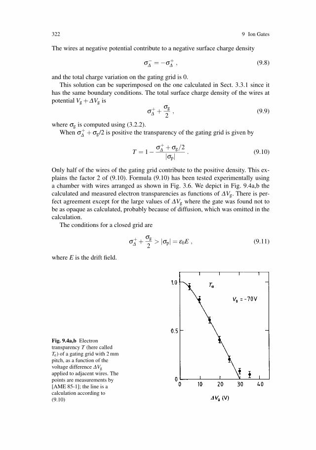
322 9 Ion Gates
The wires at negative potential contribute to a negative surface charge density
σ−Δ = −σ+
Δ , (9.8)
and the total charge variation on the gating grid is 0.This solution can be superimposed on the one calculated in Sect. 3.3.1 since it
has the same boundary conditions. The total surface charge density of the wires atpotential Vg +ΔVg is
σ+Δ +
σg
2, (9.9)
where σg is computed using (3.2.2).When σ+
Δ +σg/2 is positive the transparency of the gating grid is given by
T = 1− σ+Δ +σg/2
|σp|. (9.10)
Only half of the wires of the gating grid contribute to the positive density. This ex-plains the factor 2 of (9.10). Formula (9.10) has been tested experimentally usinga chamber with wires arranged as shown in Fig. 3.6. We depict in Fig. 9.4a,b thecalculated and measured electron transparencies as functions of ΔVg. There is per-fect agreement except for the large values of ΔVg where the gate was found not tobe as opaque as calculated, probably because of diffusion, which was omitted in thecalculation.
The conditions for a closed grid are
σ+Δ +
σg
2> |σp| = ε0E , (9.11)
where E is the drift field.
Fig. 9.4a,b Electrontransparency T (here calledTe) of a gating grid with 2 mmpitch, as a function of thevoltage difference ΔVgapplied to adjacent wires. Thepoints are measurements by[AME 85-1]; the line is acalculation according to(9.10)
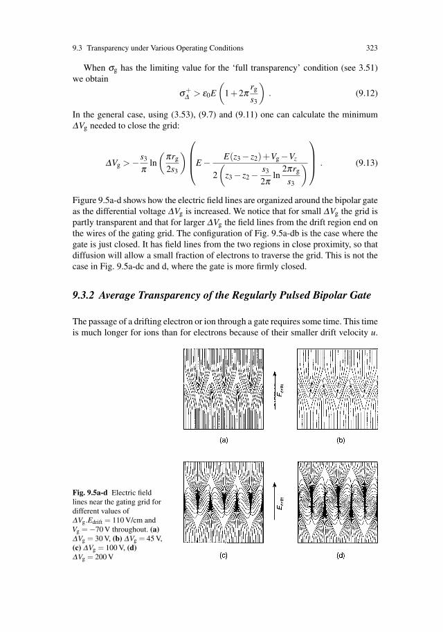
9.3 Transparency under Various Operating Conditions 323
When σg has the limiting value for the ‘full transparency’ condition (see 3.51)we obtain
σ+Δ > ε0E
(1+2π
rg
s3
). (9.12)
In the general case, using (3.53), (9.7) and (9.11) one can calculate the minimumΔVg needed to close the grid:
ΔVg > − s3
πln
(πrg
2s3
)⎛⎜⎜⎝E − E(z3 − z2)+Vg −Vz
2
(z3 − z2 −
s3
2πln
2πrg
s3
)⎞⎟⎟⎠ . (9.13)
Figure 9.5a-d shows how the electric field lines are organized around the bipolar gateas the differential voltage ΔVg is increased. We notice that for small ΔVg the grid ispartly transparent and that for larger ΔVg the field lines from the drift region end onthe wires of the gating grid. The configuration of Fig. 9.5a-db is the case where thegate is just closed. It has field lines from the two regions in close proximity, so thatdiffusion will allow a small fraction of electrons to traverse the grid. This is not thecase in Fig. 9.5a-dc and d, where the gate is more firmly closed.
9.3.2 Average Transparency of the Regularly Pulsed Bipolar Gate
The passage of a drifting electron or ion through a gate requires some time. This timeis much longer for ions than for electrons because of their smaller drift velocity u.
Fig. 9.5a-d Electric fieldlines near the gating grid fordifferent values ofΔVg.Edrift = 110 V/cm andVg = −70 V throughout. (a)ΔVg = 30 V, (b) ΔVg = 45 V,(c) ΔVg = 100 V, (d)ΔVg = 200 V
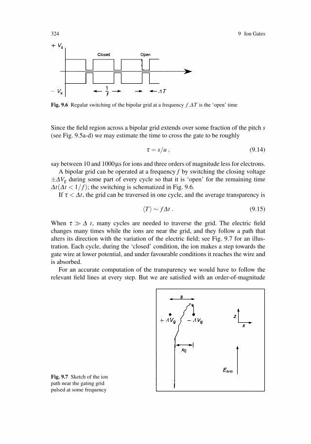
324 9 Ion Gates
Fig. 9.6 Regular switching of the bipolar grid at a frequency f .ΔT is the ‘open’ time
Since the field region across a bipolar grid extends over some fraction of the pitch s(see Fig. 9.5a-d) we may estimate the time to cross the gate to be roughly
τ = s/u , (9.14)
say between 10 and 1000μs for ions and three orders of magnitude less for electrons.A bipolar grid can be operated at a frequency f by switching the closing voltage
±ΔVg during some part of every cycle so that it is ‘open’ for the remaining timeΔ t(Δ t < 1/ f ); the switching is schematized in Fig. 9.6.
If τ < Δ t, the grid can be traversed in one cycle, and the average transparency is
〈T 〉 ∼ f Δ t . (9.15)
When τ � Δ t, many cycles are needed to traverse the grid. The electric fieldchanges many times while the ions are near the grid, and they follow a path thatalters its direction with the variation of the electric field; see Fig. 9.7 for an illus-tration. Each cycle, during the ‘closed’ condition, the ion makes a step towards thegate wire at lower potential, and under favourable conditions it reaches the wire andis absorbed.
For an accurate computation of the transparency we would have to follow therelevant field lines at every step. But we are satisfied with an order-of-magnitude
Fig. 9.7 Sketch of the ionpath near the gating gridpulsed at some frequency

9.3 Transparency under Various Operating Conditions 325
calculation, which will exhibit the main variables and their influence on the averageion transparency.
We call the effective depth of the grid S – it will be some fraction of the pitchs – and we assume that the drift field Ed acts all the time whereas the transversefield Ex between the wires of the gating grid acts only during the time the gate isclosed.
Assuming that an ion needs n cycles for the traversal of the grid,
n =S fvx
, (9.16)
it is absorbed if
x0 < n
(1f−Δ t
)vx . (9.17)
Here vz and vx are the two components of the drift velocity and x0 is the initialtransverse distance of the ion from the closest gating wire at lower potential (seeFig. 9.7).
The transparency is zero if
s <Svz
f
(1f−Δ t
)vx , (9.18)
where s is the pitch of the gating grid.We can calculate the transparency in the general case assuming that the ions are
uniformly distributed along x when they reach the region of the gating grid. Using(9.16) and (9.17) we obtain
〈T 〉 = 1− Ss
vx
vz(1− f Δ t) . (9.19)
Since the drift velocity of the ions is proportional to the electric field, the ratiobetween its components can be replaced by the ratio between the components ofthe electric field. The z component of the electric field is the drift field Ed and thex component can be approximated by 2ΔVg/s. We obtain for the time-averaged iontransparency
〈T 〉 = 1− Ss
2ΔVg
sEd(1− f Δ t) . (9.20)
Equation (9.20) shows that within the limits of our very coarse approximations, theaverage transparency is a linear function of ΔVg and the frequency f. This is alsoborne out by experiment: in Figs. 9.8 and 9.9 we see the result of measurements[AME 85-2] made with a gating grid operating under conditions similar to those ofthe ALEPH TPC. Formula (9.20) describes both curves quite well with values ofS/s between 0.4 and 0.5.

326 9 Ion Gates
Fig. 9.8 Averagetransparency 〈T 〉 for ionsthrough a bipolar grid with apitch 2 mm, which was pulsedat 100 kHz with an ‘open’time of 6μs, and a ‘closed’time of 4μs, as a function ofthe voltage difference ΔVapplied to adjacent wires. Thepoints are measured by[AME 85-2]; the straight linewas drawn to connect thepoints
9.3.3 Transparency of the Static Bipolar Gate in a TransverseMagnetic Field
A magnetic field along the main drift direction z changes the path of the electronsaccording to the parameter ωτ; see (2.6). The components ux of the drift velocityperpendicular to the magnetic field and perpendicular to the grid wires is reducedby the factor 1 +ω2τ2, whereas the drift velocity uz in the main direction stays thesame:
ux =1
1+ω2τ2 μEx ,
uz = μEz .
(9.21)
Fig. 9.9 Averagetransparency 〈T 〉 for ionsthrough a bipolar grid (pitch2 mm), which was pulsedwith ΔVg = ±45 V for aconstant ‘open’ time of 6μs,as a function of the frequency.The points are measured by[AME 85-2]; the straight linewas drawn to connect thepoints
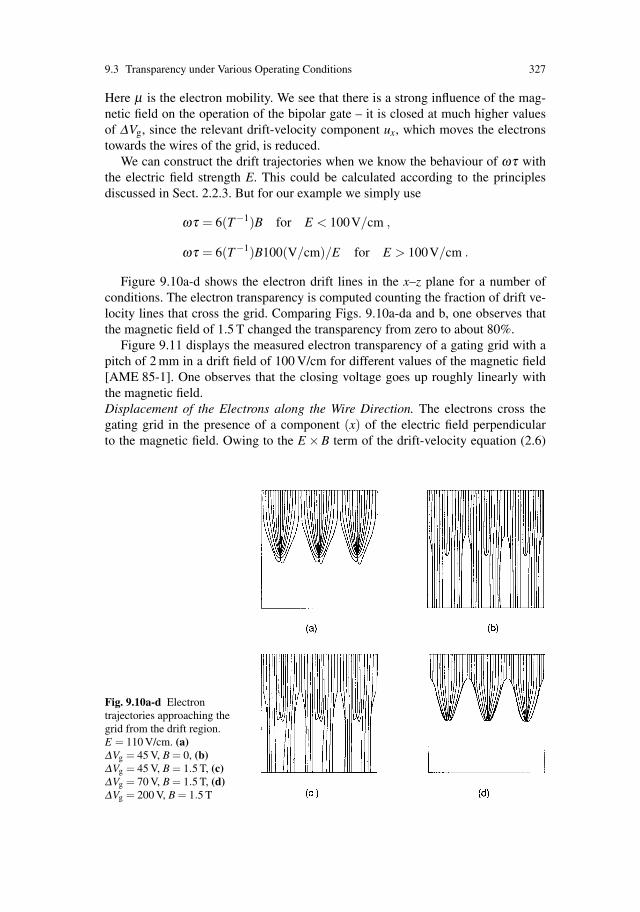
9.3 Transparency under Various Operating Conditions 327
Here μ is the electron mobility. We see that there is a strong influence of the mag-netic field on the operation of the bipolar gate – it is closed at much higher valuesof ΔVg, since the relevant drift-velocity component ux, which moves the electronstowards the wires of the grid, is reduced.
We can construct the drift trajectories when we know the behaviour of ωτ withthe electric field strength E. This could be calculated according to the principlesdiscussed in Sect. 2.2.3. But for our example we simply use
ωτ = 6(T−1)B for E < 100V/cm ,
ωτ = 6(T−1)B100(V/cm)/E for E > 100V/cm .
Figure 9.10a-d shows the electron drift lines in the x–z plane for a number ofconditions. The electron transparency is computed counting the fraction of drift ve-locity lines that cross the grid. Comparing Figs. 9.10a-da and b, one observes thatthe magnetic field of 1.5 T changed the transparency from zero to about 80%.
Figure 9.11 displays the measured electron transparency of a gating grid with apitch of 2 mm in a drift field of 100 V/cm for different values of the magnetic field[AME 85-1]. One observes that the closing voltage goes up roughly linearly withthe magnetic field.Displacement of the Electrons along the Wire Direction. The electrons cross thegating grid in the presence of a component (x) of the electric field perpendicularto the magnetic field. Owing to the E ×B term of the drift-velocity equation (2.6)
Fig. 9.10a-d Electrontrajectories approaching thegrid from the drift region.E = 110 V/cm. (a)ΔVg = 45 V, B = 0, (b)ΔVg = 45 V, B = 1.5 T, (c)ΔVg = 70 V, B = 1.5 T, (d)ΔVg = 200 V, B = 1.5 T
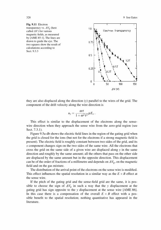
328 9 Ion Gates
Fig. 9.11 Electrontransparency vs. ΔVg (herecalled ΔV ) for variousmagnetic fields, as measuredby [AME 85-1]. The lines aredrawn to guide the eye. Thetwo squares show the result ofcalculations according toSect. 9.3.3
they are also displaced along the direction (y) parallel to the wires of the grid. Thecomponent of the drift velocity along the wire direction is
uy =ωτ
1+ω2τ2 μEx .
This effect is similar to the displacement of the electrons along the sense-wire direction when they approach the sense wire from the zero-grid region (seeSect. 7.3.1).
Figure 9.5a-db shows the electric field lines in the region of the gating grid whenthe grid is closed for the ions (but not for the electrons if a strong magnetic field ispresent). The electric field is roughly constant between two sides of the grid, and itsx component changes sign on the two sides of the same wire. All the electrons thatcross the grid on the same side of a given wire are displaced along y in the samedirection and roughly by the same amount; all the others that pass on the other sideare displaced by the same amount but in the opposite direction. This displacementcan be of the order of fractions of a millimetre and depends on ΔVg, on the magneticfield and on the gas mixture.
The distribution of the arrival point of the electrons on the sense wire is modified.This effect influences the spatial resolution in a similar way as the E ×B effect atthe sense wire.
If the pitch of the gating grid and the sense-field grid are the same, it is pos-sible to choose the sign of ΔVg in such a way that the y displacement at thegating grid has sign opposite to the y displacement at the sense wire [AME 86].In this case there is a compensation of the overall E × B effect with a pos-sible benefit to the spatial resolution; nothing quantitative has appeared in theliterature.

References 329
References
[AME 85-1] S.R. Amendolia et al., Influence of the magnetic field on the gating of a timeprojection chamber, Nucl. Instrum. Methods Phys. Res. A 234, 47 (1985)
[AME 85-2] S.R. Amendolia et al., Ion trapping properties of a synchronously gated time pro-jection chamber, Nucl. Instrum. Methods Phys. Res. A 239, 192 (1985)
[AME 86] S.R. Amendolia et al., Gating in the ALEPH time projection chamber, Nucl. In-strum. Methods Phys. Res. A 252, 403 (1986) and CERN-EF preprint 84–11 (1984)(unpublished)
[BEI 88] S.P. Beingessner, T.C. Meyer, M. Yvert, Influence of chemical trace additives onthe future ageing of the UA1 Central detector. Nucl. Instrum. Methods Phys. Res.A 272, 669 (1988)
[BRE 80] A. Breskin, G. Charpak, S. Majewski, G. Melchart, A. Peisert, F. Sauli, F. Mathy,G. Petersen, High flux operation of the gated multistep avalanche chamber, Nucl.Instrum. Methods 178, 11 (1980)
[BRY 85] D.A. Bryman et al., Gated grid system used with a time projection chamber, Nucl.Instrum. Methods Phys. Res. A 234, 42 (1985)
[KEN 84] Joel Kent, Positive ion suppression with untriggered TPC; College de FrancePreprint 84–17 (1984) (unpublished)
[NEM 83] P. Nemethy, P.J. Oddone, N. Toge, A. Ishibashi, Gated time projection chamber,Nucl. Instrum. Methods Phys. Res. 212, 273 (1983)

Chapter 10Particle Identification by Measurementof Ionization
Among the track parameters, the ionization plays a special role because it is afunction of the particle velocity, which can therefore be indirectly determinedthrough a measurement of the amount of ionization along a track. For relativisticparticles this dependence is not very strong, and therefore the amount of ionizationmust be measured accurately in order to be useful. The ionization has a very broaddistribution, and a track has to be measured on many segments (several tens to a fewhundred) in order to reach the accuracy required. Fortunately only relative values ofthe ionization need to be known between tracks of different velocities.
Whereas in Chap. 1 we dealt with the ionization phenomenon in general terms,the present chapter is devoted to a discussion of those aspects of ionization thatare important for particle identification. After an explanation of the principle weelaborate on the factors that determine the shape of the ionization curve, and theachievable accuracy. Calculated and measured particle separation powers are dis-cussed next. One section is devoted to cluster counting. Finally, the problemsencountered in practical devices are reviewed.
10.1 Principles
In a magnetic spectrometer one measures the particle momentum through the curva-ture of its track in the magnetic field. If a measurement of ionization is performed onthis track, there is the possibility of determining the particle mass, thus identifyingthe particle. The relation between momentum p and velocity v involves the mass m:
v = c2 p/E = c2 p/√
(p2c2 +m2c4) , (10.1)
where c is the velocity of light.Any quantification of ionization involves the peculiar statistics of the ionization
process. Let us recapitulate from Chap. 1 that the distribution function of the numberof electrons produced on a given track length has such a tail towards large numbersthat neither a proper mean nor a proper variance exists for the number of electrons.
W. Blum et al., Particle Detection with Drift Chambers, 331doi: 10.1007/978-3-540-76684-1 10, c© Springer-Verlag Berlin Heidelberg 2008
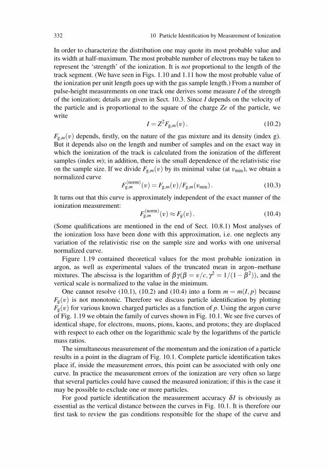
332 10 Particle Identification by Measurement of Ionization
In order to characterize the distribution one may quote its most probable value andits width at half-maximum. The most probable number of electrons may be taken torepresent the ‘strength’ of the ionization. It is not proportional to the length of thetrack segment. (We have seen in Figs. 1.10 and 1.11 how the most probable value ofthe ionization per unit length goes up with the gas sample length.) From a number ofpulse-height measurements on one track one derives some measure I of the strengthof the ionization; details are given in Sect. 10.3. Since I depends on the velocity ofthe particle and is proportional to the square of the charge Ze of the particle, wewrite
I = Z2Fg,m(v) . (10.2)
Fg,m(v) depends, firstly, on the nature of the gas mixture and its density (index g).But it depends also on the length and number of samples and on the exact way inwhich the ionization of the track is calculated from the ionization of the differentsamples (index m); in addition, there is the small dependence of the relativistic riseon the sample size. If we divide Fg,m(v) by its minimal value (at vmin), we obtain anormalized curve
F(norm)g,m (v) = Fg,m(v)/Fg,m(vmin) . (10.3)
It turns out that this curve is approximately independent of the exact manner of theionization measurement:
F(norm)g,m (v) ≈ Fg(v) . (10.4)
(Some qualifications are mentioned in the end of Sect. 10.8.1) Most analyses ofthe ionization loss have been done with this approximation, i.e. one neglects anyvariation of the relativistic rise on the sample size and works with one universalnormalized curve.
Figure 1.19 contained theoretical values for the most probable ionization inargon, as well as experimental values of the truncated mean in argon–methanemixtures. The abscissa is the logarithm of βγ(β = v/c,γ2 = 1/(1−β 2)), and thevertical scale is normalized to the value in the minimum.
One cannot resolve (10.1), (10.2) and (10.4) into a form m = m(I, p) becauseFg(v) is not monotonic. Therefore we discuss particle identification by plottingFg(v) for various known charged particles as a function of p. Using the argon curveof Fig. 1.19 we obtain the family of curves shown in Fig. 10.1. We see five curves ofidentical shape, for electrons, muons, pions, kaons, and protons; they are displacedwith respect to each other on the logarithmic scale by the logarithms of the particlemass ratios.
The simultaneous measurement of the momentum and the ionization of a particleresults in a point in the diagram of Fig. 10.1. Complete particle identification takesplace if, inside the measurement errors, this point can be associated with only onecurve. In practice the measurement errors of the ionization are very often so largethat several particles could have caused the measured ionization; if this is the case itmay be possible to exclude one or more particles.
For good particle identification the measurement accuracy δ I is obviously asessential as the vertical distance between the curves in Fig. 10.1. It is therefore ourfirst task to review the gas conditions responsible for the shape of the curve and

10.1 Principles 333
Fig. 10.1 Most probable values of the ionization (normalized to the minimum value) in argon atordinary density as function of the momenta of the known stable charged particles
in particular for the amount of the relativistic rise. Then we have to understand thecircumstances that have an influence on δ I, and which value of δ I can be reachedin a given apparatus. The ratio of the accuracy over the relativistic rise characterizesthe particle separation power.
But before going into these details let us make an estimate of what we can expectfrom this method of particle identification. Imagine some drift chamber with a rel-ative accuracy of δ I/I = 12% FWHM (5% r.m.s.). If we assume that a respectabledegree of identification is already achievable on a curve that is only twice this r.m.s.value away from any other one, if we remove the muon curve (because it is hope-lessly close to the pion curve and because muons can be well identified with othermethods), and if, finally, we assume that the error of the momentum measurement isnegligible, then we can redraw those branches of the curves in Fig. 10.1 that wouldallow a respectable degree of particle identification in argon. The result is seen inFig. 10.2.
Under the assumed circumstances, these particles could be identified in theranges shown in Table 10.1. It is characteristic of the complicated shape of the ion-ization curve that there are certain bands of overlap in which unique identification isimpossible. A useful separation between kaons and protons at high momenta wouldrequire the measurement accuracy for the ionization to be δ I/I = 8.5% FWHMor better (in argon at normal density). Such values have actually been attained byspecialized particle identifiers, see Sect. 10.8.
After having described the principle of particle identification based on theamount of ionization along a given length of track we should also mention the pos-sibility based on the frequency of ionization along the track. If we were to count the

334 10 Particle Identification by Measurement of Ionization
Fig. 10.2 The same asFig. 10.1 with all lines left outthat either belong to a muonor that have a neighbouringline closer than 10% inionization (corresponding to aseparation of 2 standarddeviations when the r.m.s.accuracy is 5%)
Table 10.1 Momentum ranges above 0.1 GeV/c for a 2 σ identification of particles in argon(normal density), for two measuring accuracies of the ionization (μ’s removed)
Particle Momentum ranges (GeV/c)
δ I/I = 5% r.m.s.e 0.17–0.4 0.6–0.8 1.3–19π (0.1)–0.12 0.16–0.8 2.7–19K (0.1)–0.4 0.6–0.8p (0.1)–0.8 1.1–1.5δ I/I = 3.5% r.m.s.e 0.16–0.5 0.6–0.9 1.1–30π (0.1)–0.13 0.16–0.9 2.2–30K (0.1)–0.5 0.6–0.9 6–46p (0.1)–0.9 1.1–1.5 6–46
number of ionization clusters rather than the amount of ionization on some tracklength, there would be a profit in the statistical accuracy. A brief description of thisinteresting method is given in Sect. 10.6.
Much easier than the identification of the known particles would be the recog-nition of a stable quark with charge e/3 or 2e/3, because it would create only 1/9or 4/9 of the normal ionization density. Quarks aside, one recognizes that relativelysmall differences in δ I/I may be decisive for particle identification. Therefore wemust study in some detail how the shape of the ionization curve and the achievableaccuracy depend on the parameters of the drift chamber.
10.2 Shape of the Ionization Curve
We recall from Chap. 1 that the curve reaches its minimum near βγ = 4. The shapeof a curve that has been normalized to this minimum is characterized by the heightof the plateau (‘amount of relativistic rise’, R, above the minimum) and by the value
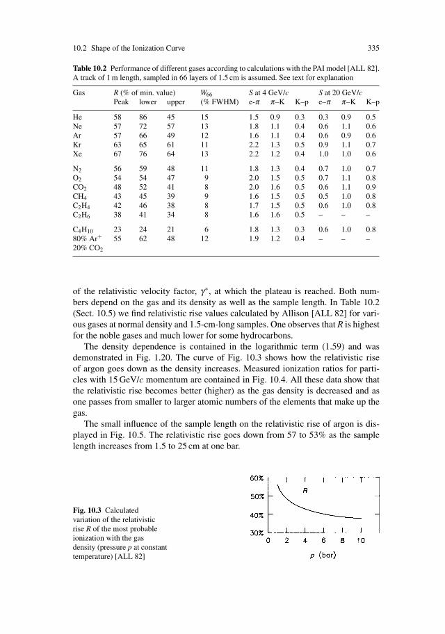
10.2 Shape of the Ionization Curve 335
Table 10.2 Performance of different gases according to calculations with the PAI model [ALL 82].A track of 1 m length, sampled in 66 layers of 1.5 cm is assumed. See text for explanation
Gas R (% of min. value) W66 S at 4 GeV/c S at 20 GeV/cPeak lower upper (% FWHM) e-π π–K K–p e–π π–K K–p
He 58 86 45 15 1.5 0.9 0.3 0.3 0.9 0.5Ne 57 72 57 13 1.8 1.1 0.4 0.6 1.1 0.6Ar 57 66 49 12 1.6 1.1 0.4 0.6 0.9 0.6Kr 63 65 61 11 2.2 1.3 0.5 0.9 1.1 0.7Xe 67 76 64 13 2.2 1.2 0.4 1.0 1.0 0.6
N2 56 59 48 11 1.8 1.3 0.4 0.7 1.0 0.7O2 54 54 47 9 2.0 1.5 0.5 0.7 1.1 0.8CO2 48 52 41 8 2.0 1.6 0.5 0.6 1.1 0.9CH4 43 45 39 9 1.6 1.5 0.5 0.5 1.0 0.8C2H4 42 46 38 8 1.7 1.5 0.5 0.6 1.0 0.8C2H6 38 41 34 8 1.6 1.6 0.5 – – –
C4H10 23 24 21 6 1.8 1.3 0.3 0.6 1.0 0.880% Ar+ 55 62 48 12 1.9 1.2 0.4 – – –20% CO2
of the relativistic velocity factor, γ∗, at which the plateau is reached. Both num-bers depend on the gas and its density as well as the sample length. In Table 10.2(Sect. 10.5) we find relativistic rise values calculated by Allison [ALL 82] for vari-ous gases at normal density and 1.5-cm-long samples. One observes that R is highestfor the noble gases and much lower for some hydrocarbons.
The density dependence is contained in the logarithmic term (1.59) and wasdemonstrated in Fig. 1.20. The curve of Fig. 10.3 shows how the relativistic riseof argon goes down as the density increases. Measured ionization ratios for parti-cles with 15 GeV/c momentum are contained in Fig. 10.4. All these data show thatthe relativistic rise becomes better (higher) as the gas density is decreased and asone passes from smaller to larger atomic numbers of the elements that make up thegas.
The small influence of the sample length on the relativistic rise of argon is dis-played in Fig. 10.5. The relativistic rise goes down from 57 to 53% as the samplelength increases from 1.5 to 25 cm at one bar.
Fig. 10.3 Calculatedvariation of the relativisticrise R of the most probableionization with the gasdensity (pressure p at constanttemperature) [ALL 82]
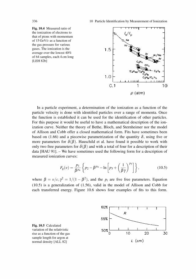
336 10 Particle Identification by Measurement of Ionization
Fig. 10.4 Measured ratio ofthe ionization of electrons tothat of pions with momentumof 15 GeV/c as a function ofthe gas pressure for variousgases. The ionization is theaverage over the lowest 40%of 64 samples, each 4 cm long[LEH 82b]
In a particle experiment, a determination of the ionization as a function of theparticle velocity is done with identified particles over a range of momenta. Oncethe function is established it can be used for the identification of other particles.For this purpose it would be useful to have a mathematical description of the ion-ization curve. Neither the theory of Bethe, Bloch, and Sternheimer nor the modelof Allison and Cobb offer a closed mathematical form. Fits have sometimes beenbased on (1.66) and a piecewise parametrization of the quantity δ , using five ormore parameters for δ (β ). Hauschild et al. have found it possible to work withonly two free parameters for δ (β ) and with a total of four for a description of theirdata [HAU 91]. – We have sometimes used the following form for a description ofmeasured ionization curves:
Fg(v) =p1
β p4
{p2 −β p4 − ln
[p3 +
(1
βγ
)p5]}
, (10.5)
where β = v/c,γ2 = 1/(1 − β 2), and the pi are five free parameters. Equation
(10.5) is a generalization of (1.56), valid in the model of Allison and Cobb foreach transferred energy. Figure 10.6 shows four examples of fits to this form.
Fig. 10.5 Calculatedvariation of the relativisticrise as a function of the gassample length for argon atnormal density [ALL 82]
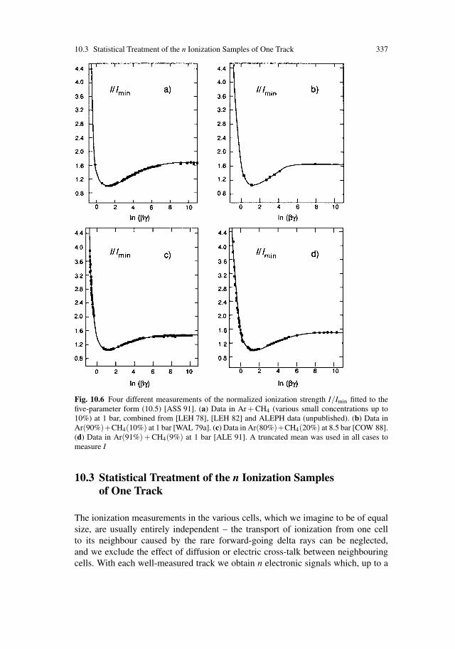
10.3 Statistical Treatment of the n Ionization Samples of One Track 337
Fig. 10.6 Four different measurements of the normalized ionization strength I/Imin fitted to thefive-parameter form (10.5) [ASS 91]. (a) Data in Ar + CH4 (various small concentrations up to10%) at 1 bar, combined from [LEH 78], [LEH 82] and ALEPH data (unpublished). (b) Data inAr(90%)+CH4(10%) at 1 bar [WAL 79a]. (c) Data in Ar(80%)+CH4(20%) at 8.5 bar [COW 88].(d) Data in Ar(91%) + CH4(9%) at 1 bar [ALE 91]. A truncated mean was used in all cases tomeasure I
10.3 Statistical Treatment of the n Ionization Samplesof One Track
The ionization measurements in the various cells, which we imagine to be of equalsize, are usually entirely independent – the transport of ionization from one cellto its neighbour caused by the rare forward-going delta rays can be neglected,and we exclude the effect of diffusion or electric cross-talk between neighbouringcells. With each well-measured track we obtain n electronic signals which, up to a

338 10 Particle Identification by Measurement of Ionization
common constant, represent n sample values of the ionization distribution in a cell.The task is to derive from them a suitable estimator for the strength of the ionizationin the cell.
The most straightforward, the average of all n values, is a bad estimator whichfluctuates a lot from track to track, because the underlying mathematical ionizationdistribution has no finite average and no finite variance (see (1.33). A good estima-tor is either derived from a fit to the shape of the measured distribution or from asubsample excluding the very high measured values.
In many cases one knows the shape of the signal distribution, f (S)dS, up to ascale parameter λ that characterizes the ionization strength. The n signals S1, . . . ,Sn
are to be used for a determination of λ . Let λ be fixed to 1 for the normalizedreference distribution f1(S)dS. Then there is a family of normalized distributions
fλ (S)dS = (1/λ ) f1(S/λ )dS , (10.6)
and one must find out which curve fits best the n signal values. The most efficientmethod to achieve this is the maximum-likelihood method. It requires one to maxi-mize with respect to λ the likelihood function
L = ∏i(1/λ ) f1(Si/λ ) , (10.7)
where the product runs over all n samples. The result is a λ0 and its error δλ0. Onemay take λ to represent the most probable signal of the distribution; then λ0 ±δλ0
is the most probable signal measured for the track at hand.So far, it has been assumed that the shape of the ionization curve is the same (at a
given gas length) for all ionization strengths, i.e. particle velocities. For very smallgas lengths this is not really true (see Fig. 1.21). In this case one needs a table ofdifferent curves rather than the simple family (10.6). The rest goes as before.
For a general treatment of parameter estimation, the likelihood method, or theconcept of efficiency, the reader is referred to a textbook on statistics, e.g. Cramer[CRA 51] or Fisz [FIS 58] or Eadie et al. [EAD 71].
If one does not know the shape of the signal distribution beforehand, one mayuse a simplified method, the method of “the truncated mean”. It is characterized bya cut-off parameter η between 0 and 1. The estimator 〈S〉η for the signal strength isthe average of the ηn lowest values among the n signals Si:
〈S〉η =1m
m
∑1
S j ,
where m is the integer closest to ηn, and the sum extends over the lowest m elementsof the ordered full sample (S j ≤ S j+1 for all j = 1, . . . ,n− 1). The quantity thatmatters is the fluctuation of 〈S〉η divided by its value; if for a typical ionizationdistribution one simulates with the Monte Carlo method the measurement of manytracks in order to determine the best η , one finds a shallow minimum of this quantityas a function of η between 0.35 and 0.75. In this range of η it is an empirical factthat the values of 〈S〉η are distributed almost like a Gaussian. In many practical

10.4 Accuracy of the Ionization Measurement 339
experiments the method of the truncated mean was the method of choice, because ofits simplicity and because the likelihood method had not given recognizably betterresults. From a theoretical point of view, the likelihood method should be the bestas it makes use of all the available information.
Whatever the exact form of the estimator, we assume that it is a measure ofthe amount of ionization, which obeys (10.2), and that the approximation (10.4) issufficiently well fulfilled for a practical analysis.
10.4 Accuracy of the Ionization Measurement
We have to understand how the accuracy of the ionization measurement of one trackvaries with its length L and the number n of samples, with the nature of the gas andwith its pressure p. Since the distribution in a given gap with length x = L/n dependsonly on the cluster-size distribution and on the number of primary interactions inthe gap, the ionization distribution varies with the density (or pressure at constanttemperature) in the same way as it does with x, and therefore the width W of thedistribution depends on x and p through their product xp. The relative accuracy willtherefore be of the form
δ II
= f (xp, n, gas) or g(Lp, n, gas) .
10.4.1 Variation with n and x
If a track of length L is sampled on n small pieces of length x, we may expect thatthe accuracy δ Imp in the determination of the most probable-value improves whenwe increase n and L, keeping x fixed. Different values of n may arise for tracks inone event, depending on the number of samples lost because of overlapping tracks.If the basic distribution of the ionization gathered in one piece x were well behavedin the sense of having a mean and a variance – a prerequisite for an application ofthe central-limit theorem of statistics – then the accuracy would become better withincreasing n and L according to the law δ Imp ∼ 1/
√n in the limit of large n. It turns
out that with the very special cluster-size distribution of Chap. 1 the gain is morelike n−0.46 for practical values of n when dealing with a maximum-likelihood fit forthe most probable value [ALL 80]. Walenta and co-workers obtained n−0.43 whendealing with the average 〈I〉40 of the lowest 40% [WAL 79]. The differences in theexponent seem to be small but they count for large n! In any event one deals herewith empirical relations that have not been justified on mathematical grounds.
If we vary L and x simultaneously, keeping n fixed, we must consider how thewidth of the ionization distribution changes with the size x of the individual sample.The variation of L and x at constant n could be produced by increasing the gaspressure in a suitable multiwire drift chamber.

340 10 Particle Identification by Measurement of Ionization
As the gap is made larger, W decreases. This has been treated in Chap. 1 (see thediscussion around (1.37) and Fig. 1.10). The experiments suggest a power behaviourof the relative width W on a single gap, which varies like
(W/Imp)1 : (W/Imp)2 = [(px)1 : (px)2]k = [(pL)1 : (pL)2]k (10.8)
(Imp = most probable ionization). Based on the PAI model and supported by experi-mental data one finds that k = −0.32 [ALL 80].
Next we keep the length L = nx fixed and increase n, reducing x. Now there is anet gain in the accuracy δ I proportional to
n−0.14 or n−0.11
because the better accuracy from the increase of n is partly offset by the worseningfrom the decrease in x.
Although there is agreement between the different authors about these facts,they disagree about the question down to what subdivision this rule holds. WhereasAllison and Cobb, on the basis of their theory and in accordance with the above, rec-ommend sampling the ionization as finely as possible [ALL 80], Walenta suggeststhat below 5 cm bar in argon the improvement is negligible [WAL 79]. Lehraus etal., from a more practical point of view, argue similarly [LEH 82a]. It must be saidthat, at the time, such fine samples had not been systematically explored. More re-cently the ALEPH and the DELPHI TPCs, working at normal gas density and with4 mm sense-wire spacing, sample remarkably thin gas layers. Figure 10.7 shows anALEPH study [ASS 90] in which lepton tracks from e+e− interactions were an-alyzed by adding the signals from neighbouring sense wires, thus varying n andx at fixed L. Though not quite reaching the theoretical prediction (see below), themeasured accuracy as a function of n lends some support to the idea that fine subdi-visions down to half a cm bar may still increase the accuracy.
10.4.2 Variation with the Particle Velocity
We have seen how the single-gap width W is reduced by multiple measurements.The value of W itself results from the summation over the cluster-size distribution
Fig. 10.7 Ionizationresolution at constant tracklength as a function of thesample length. Crosses:measured in the ALEPH-TPC(average track length 140 cm,argon (91%) + methane (9%)at 1 bar, diffusion < 1.4 mmr.m.s.). Line: prediction ofAllison and Cobb, our (10.9)
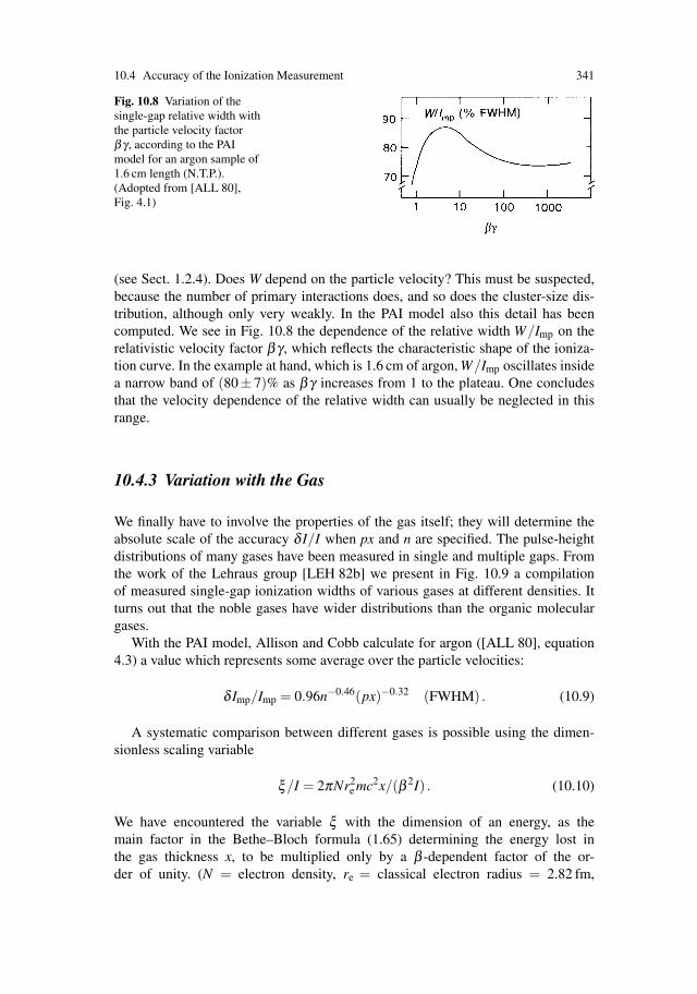
10.4 Accuracy of the Ionization Measurement 341
Fig. 10.8 Variation of thesingle-gap relative width withthe particle velocity factorβγ , according to the PAImodel for an argon sample of1.6 cm length (N.T.P.).(Adopted from [ALL 80],Fig. 4.1)
(see Sect. 1.2.4). Does W depend on the particle velocity? This must be suspected,because the number of primary interactions does, and so does the cluster-size dis-tribution, although only very weakly. In the PAI model also this detail has beencomputed. We see in Fig. 10.8 the dependence of the relative width W/Imp on therelativistic velocity factor βγ , which reflects the characteristic shape of the ioniza-tion curve. In the example at hand, which is 1.6 cm of argon, W/Imp oscillates insidea narrow band of (80± 7)% as βγ increases from 1 to the plateau. One concludesthat the velocity dependence of the relative width can usually be neglected in thisrange.
10.4.3 Variation with the Gas
We finally have to involve the properties of the gas itself; they will determine theabsolute scale of the accuracy δ I/I when px and n are specified. The pulse-heightdistributions of many gases have been measured in single and multiple gaps. Fromthe work of the Lehraus group [LEH 82b] we present in Fig. 10.9 a compilationof measured single-gap ionization widths of various gases at different densities. Itturns out that the noble gases have wider distributions than the organic moleculargases.
With the PAI model, Allison and Cobb calculate for argon ([ALL 80], equation4.3) a value which represents some average over the particle velocities:
δ Imp/Imp = 0.96n−0.46(px)−0.32 (FWHM) . (10.9)
A systematic comparison between different gases is possible using the dimen-sionless scaling variable
ξ/I = 2πNr2e mc2x/(β 2I) . (10.10)
We have encountered the variable ξ with the dimension of an energy, as themain factor in the Bethe–Bloch formula (1.65) determining the energy lost inthe gas thickness x, to be multiplied only by a β -dependent factor of the or-der of unity. (N = electron density, re = classical electron radius = 2.82 fm,

342 10 Particle Identification by Measurement of Ionization
Fig. 10.9 Single-gap resolution measured for various gases and pressures [LEH 82b] as a functionof the product of pressure p and sample length x
mc2 = rest energy of the electron, β = particle velocity in units of the velocityof light.) We have also met the variable ξ as the scaling factor (1.49) in the Landaudistribution.
The mean ionization potential I is the only constant in the Bethe–Bloch formulathat characterizes the gas; see Table 1.3. The ratio ξ/I will be roughly proportionalto the number of electrons liberated over the distance x, and therefore it is plausiblethat it might serve in a comparison of accuracies δ I/I. For β = 1 and gas layers of1 cm, ξ/I takes on the values 0.32, 0.50, 0.62, 0.65, and 0.70 for the noble gasesHe, Ne, Ar, Kr, and Xe at N.T.P., respectively.
From the work of Ermilova, Kotenko and Merzon [ERM 77], Fig. 10.10 con-tains calculated values of the width of the ionization distribution in a single gap, forvarious noble gases, plotted as a function of the ratio ξ/I. The full width at halfmaximum is expressed in units of ξ . We notice that the points of the different gasesand sample lengths x fall roughly on one universal curve, which only depends onξ/I. We also notice that for ξ/I near 1 the theoretical predictions for the width ofLandau and Blunck–Leisegang (see Sect. 1.2.5) differ by half an order of magni-

10.4 Accuracy of the Ionization Measurement 343
Fig. 10.10 The widths of the ionization distributions in units of ξ for the noble gases, calculatedfor various sample lengths by Ermilova et al., plotted as a function of ξ/I (10.10) [ERM 77]. Thepoints calculated by a Monte Carlo method follow a universal dependence of ξ/I
tude; on the other hand, the Monte Carlo calculation of Ermilova et al., which isvery similar to the subsequent PAI model, accurately predicts the measured widths.The three calculations and the experimental points fall generally together only forratios ξ/I larger than about 50.
Using the universal variable ξ/I Allison and Cobb generalized relation (10.9) forall gases:
δ Imp/Imp = 0.81n−0.46(ξ/I)−0.32 (FWHM) . (10.11)
It should be emphasized that this formula has not yet been tested experimentally ina systematic comparison between different gases. The value of the constant is equalto the value of 0.96(ξ/I)0.32 for 1 cm of argon.
In (10.11) the length of the device is contained in ξ and n, the gas pres-sure in ξ . If we want to make their influence more visible we may calculatefrom (10.9) the relative accuracy obtainable with a device 1 m long containingargon gas at N.T.P., and 100 samplings; the result is δ Imp/Imp = 0.115. Thevalue of ξ varies between different gases in the ratio of their atomic chargenumber Z. Therefore we have for the general case of a gas, characterized by Zand I,
δ Imp
Imp= 0.115
(1mbar
Lp
)0.32(ZArIZIAr
)0.32(100n
)0.14
(FWHM) , (10.12)

344 10 Particle Identification by Measurement of Ionization
where L is the length, p the gas pressure and n the number of samplings; Iindicates the average ionization potential as used in the Bethe–Blochformula.
10.5 Particle Separation
In order to judge the power of particle separation for a certain gas and wire arrange-ment we must combine the results of Sects. 10.2 and 10.4. Generally speaking, thefigure of interest is the ratio δ I/(IR). The noble gases have a wider pulse-heightdistribution but also a larger relativistic rise, compared to the hydrocarbons investi-gated. The same compensation is at work with the gas density: as the accuracy δ I/Ibecomes better with higher density, the relativistic rise R gets worse; in addition thesaturation of the plateau starts at a lower γ∗. Finer sampling is an advantage evenin the approximation (10.4). In addition, there is the tiny increase, if any, of R withfiner samples.
The performance of various gases, according to calculations with the PAI model,is compared in Table 10.2 [ALL 82]. These results refer to normal density and totracks 1 m long, which are sampled in 1.5 cm intervals. The relativistic rise R isindicated for the most probable value of the ionization distribution and for the lowerand upper points at half maximum. The full width W66 of the ionization determina-tion derivable from a maximum-likelihood fit to all 66 measurements is also shown.The last 6 columns contain particle-pair separation powers S, i.e. for a given pair ofparticles at some momentum the difference of the peak positions, divided by W66.Remarkably, the separation powers of different gases are very similar.
Measurements of the separation power for various gases and pressures have beenperformed in a beam of identified particles by Lehraus et al. [LEH 82b]. In their de-tector with 64 cells, each 4 cm long, they determined simultaneously the differencebetween the ionization of electrons, pions and protons and the accuracy δ I (r.m.s.width of the distribution). The gas and its pressure were varied. Considering the sep-aration of these particles at 15 GeV/c, the results are expressed as the ratios D/σ ,equal to
〈Iπ〉40 −〈I p〉40
δ 〈Iπ〉40or
〈Ie〉40 −〈Iπ〉40
δ 〈Iπ〉40, (10.13)
plotted against pressure in Fig. 10.11. This diagram contains a summary of muchcareful and systematic study. We observe a general decrease below 1 bar and oftena decrease above 2 bar, although there are several gas mixtures, where the pion–proton separation increases up to 4 bar. In any event, the values of the ratios stay thesame within a few tenths between 1 and 4 bar.
Single-gap measurements in three gases were reported by Walenta et al. [WAL 79]at 3.5 GeV/c. The measured ratio of peak displacement over the full width is plottedagainst pressure in Fig. 10.12. An increase in separation power can be observed atpressures above 1 bar. The overall picture is that with some gases a profit can bemade by going above 1 bar.

10.6 Cluster Counting 345
Fig. 10.11 Pressure dependence of the resolving power (10.13) for various argon gas mixtures, asmeasured by [LEH 82a] at 15 GeV/c. The numbers close to the chemical symbols of the quenchgases refer to the concentrations; for example, 20CH4 means 80% Ar+20%CH4
10.6 Cluster Counting
The statistical distribution of the number of ionization electrons produced on a giventrack length has a width W (measured at one half of the maximal probability), whichwas plotted relative to the most probable ionization Imp in Fig. 1.12 as a functionof the track length. This width is determined by the fluctuation in the number ofprimary clusters that occur over this length and by the fluctuation in the cluster size.It is the latter that dominates; for example, there are 28 primary clusters on 1 cmbar of argon whose Poissonian fluctuation is only 44% FWHM, whereas W/Imp isapproximately equal to 1, and for 10 cm bar of argon, the corresponding numbers are
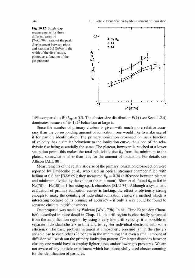
346 10 Particle Identification by Measurement of Ionization
Fig. 10.12 Single-gapmeasurements for threedifferent gases by[WAL 79a]: ratio of the peakdisplacement between pionsand kaons at 3.5 GeV/c to thewidth of the distribution,plotted as a function of thegas pressure
14% compared to W/Imp ≈ 0.5. The cluster-size distribution P(k) (see Sect. 1.2.4)dominates because of its 1/k2 behaviour at large k.
Since the number of primary clusters is given with much more relative accu-racy than the corresponding amount of ionization, one would like to make use ofit for particle identification. The primary ionization cross-section, as a functionof velocity, has a similar behaviour to the ionization curve, the slope of the rela-tivistic rise being essentially the same. The plateau, however, is reached at a lowersaturation point; this makes the total relativistic rise Rp from the minimum to theplateau somewhat smaller than it is for the amount of ionization. For details seeAllison [ALL 80].
Measurements of the relativistic rise of the primary ionization cross-section werereported by Davidenko et al., who used an optical streamer chamber filled withhelium at 0.6 bar [DAV 69]; they measured Rp = 0.38 (difference between plateauand minimum divided by the value at the minimum). Blum et al. found Rp = 0.6 inNe(70) + He(30) at 1 bar using spark chambers [BLU 74]. Although a systematicevaluation of primary ionization curves is lacking, the effect is obviously strongenough to make the counting of individual ionization clusters a method which isinteresting because of its promise of accuracy – if only a way could be found toseparate clusters in drift chambers.
One proposal was made by Walenta [WAL 79b]. In his ‘Time Expansion Cham-ber’, described in more detail in Chap. 11, the drift region is electrically separatedfrom the amplification region; by using a very low drift velocity, it is possible toseparate individual clusters in time and to register individual electrons with someefficiency. The basic problem in argon at atmospheric pressure is that the clustersare so close to each other (28 per cm in the minimum) that even a small amount ofdiffusion will wash out the primary ionization pattern. For larger distances betweenclusters one would have to employ lighter gases and/or lower gas pressures. We arenot aware of any particle experiment which has successfully used cluster countingfor the identification of particles.

10.7 Ionization Measurement in Practice 347
10.7 Ionization Measurement in Practice
The large multiwire drift chambers provide many coordinate measurements on eachtrack, and more often than not this includes recording the wire pulse heights. Theseare then a measure of the ionization density of each track segment, provided thechamber is operated in the proportional regime. In the universal detectors the parti-cles go in all directions, and their ionization is sampled in different ways, dependingon how the track is oriented with respect to the wire array that records it.
There are also more specialized drift chambers, which were built with the expresspurpose of particle identification behind fixed-target experiments. There, the parti-cles travel generally into one main direction, which makes the ionization samplingmuch more uniform than it is in the universal detectors.
For good ionization measurements a balance has to be found between two con-flicting requirements. On the one hand, the wire gain must be kept small in orderto have a signal accurately proportional to the incoming ionization charge. Whenthe gain is too large, the amplification will drop when the incoming charges areconcentrated along a short piece of wire, owing to space charge near the wire (seeSect. 4.5), resulting in a gain variation with the amount of diffusion and the track-wire angle. Furthermore, the positive ions created in the wire avalanches penetrateto a certain extent into the drift space, where they cause field and hence track andgain distortions. On the other hand, large signals are required for the coordinatemeasurement in order to overcome the electronic amplifier noise; this is particularlyimportant for coordinate measurements along the wire, using charge division.
The pulse integration must work in such a way that the result is exactly pro-portional to the collected charge, and especially that it is independent of the lengthof the pulse. Otherwise it has to be corrected by a function of the track angle andthe drift length, which both have an influence on the pulse length. In order to havea clean pulse integration, overlapping tracks must be eliminated with some safetymargin. The number of signals on a track in the middle of a jet of other particles cantherefore be considerably reduced. It is not uncommon that in a large drift chamberthe average number of signals is only little more than one half of the number ofwires that could in principle measure a track.
In order to derive a meaningful ionization of a track, truly independent of all theexternal circumstances of the measurement, a number of calibrations and correc-tions are required at the percentage level of accuracy. These may be grouped in twocategories, according to whether or not they depend on the track parameters.
10.7.1 Track-Independent Corrections
Without going into the details, we just mention the following effects which changethe apparent ionization and therefore have to be kept under control: gas density(pressure and temperature), concentration ratios of the components, electron attach-ment, base line and pedestal shift of the electronic channels.
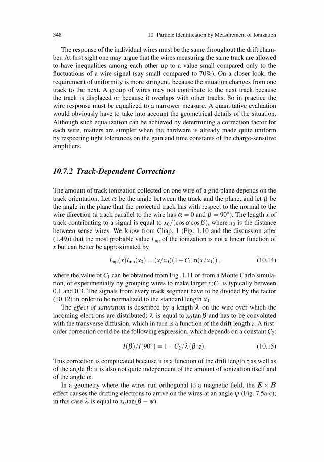
348 10 Particle Identification by Measurement of Ionization
The response of the individual wires must be the same throughout the drift cham-ber. At first sight one may argue that the wires measuring the same track are allowedto have inequalities among each other up to a value small compared only to thefluctuations of a wire signal (say small compared to 70%). On a closer look, therequirement of uniformity is more stringent, because the situation changes from onetrack to the next. A group of wires may not contribute to the next track becausethe track is displaced or because it overlaps with other tracks. So in practice thewire response must be equalized to a narrower measure. A quantitative evaluationwould obviously have to take into account the geometrical details of the situation.Although such equalization can be achieved by determining a correction factor foreach wire, matters are simpler when the hardware is already made quite uniformby respecting tight tolerances on the gain and time constants of the charge-sensitiveamplifiers.
10.7.2 Track-Dependent Corrections
The amount of track ionization collected on one wire of a grid plane depends on thetrack orientation. Let α be the angle between the track and the plane, and let β bethe angle in the plane that the projected track has with respect to the normal to thewire direction (a track parallel to the wire has α = 0 and β = 90◦). The length x oftrack contributing to a signal is equal to x0/(cosα cosβ ), where x0 is the distancebetween sense wires. We know from Chap. 1 (Fig. 1.10 and the discussion after(1.49)) that the most probable value Imp of the ionization is not a linear function ofx but can better be approximated by
Imp(x)Imp(x0) = (x/x0)(1+C1 ln(x/x0)) , (10.14)
where the value of C1 can be obtained from Fig. 1.11 or from a Monte Carlo simula-tion, or experimentally by grouping wires to make larger x;C1 is typically between0.1 and 0.3. The signals from every track segment have to be divided by the factor(10.12) in order to be normalized to the standard length x0.
The effect of saturation is described by a length λ on the wire over which theincoming electrons are distributed; λ is equal to x0 tanβ and has to be convolutedwith the transverse diffusion, which in turn is a function of the drift length z. A first-order correction could be the following expression, which depends on a constant C2:
I(β )/I(90◦) = 1−C2/λ (β ,z) . (10.15)
This correction is complicated because it is a function of the drift length z as well asof the angle β ; it is also not quite independent of the amount of ionization itself andof the angle α .
In a geometry where the wires run orthogonal to a magnetic field, the E ×Beffect causes the drifting electrons to arrive on the wires at an angle ψ (Fig. 7.5a-c);in this case λ is equal to x0 tan(β −ψ).

10.8 Performance Achieved in Existing Detectors 349
The signal attenuation due to electron attachment requires a correction whichdepends on the drift length z through a constant C3:
I(z) = I(0)e−C3 z . (10.16)
Electronic cross-talk between wires can give rise to an α-dependent correc-tion because the small ‘illegal’ pulses induced on neighbouring wires are prompt,whereas the normal signal develops according to the arrival time of the electrons.The time differences between the normal and the small induced pulses depend on αand will give rise to a variation in the pulse integration.
The corrections discussed above are all interconnected, and it is difficult to isolatethe individual effects. In fact, we do not know a particle experiment in which sucha programme has been successfully completed in all details. Nonetheless, with thecorrections applied, in practice it has usually been possible for the determination oftrack ionization to reach a level of accuracy that is not far from that predicted by(10.9). The reader who is interested in more details of the correction procedure isreferred to the articles by the groups of ISIS2 [ALL 82, ALL 84], OPAL [BRE 87,HAU 91], CRISIS [TOO 88] and ALEPH [ATW 91].
10.8 Performance Achieved in Existing Detectors
It is appropriate now to describe a small number of wire chambers used in particleexperiments and to compare their ionization-measuring capability with the theory.Although a systematic discussion of existing drift chambers begins in Chap. 11, wewant to include a few devices here as examples in the context of ionization measure-ment. We distinguish specialized chambers and universal detectors. The emphasisis on measurements in the region of the relativistic rise.
10.8.1 Wire Chambers Specialized to Measure Track Ionization
As the progress in accelerator technology made fixed-target experiments possiblein particle beams with momenta up to one hundred GeV/c or more, the relativisticrise of the ionization in gases was put to the service of identifying the secondaryparticles. The first and largest such undertaking was the External Particle Identi-fier (‘EPI’) behind the Big European Bubble Chamber (‘BEBC’). It consisted of astack of 64 rectangular chambers, each 1 m high, 2 m wide and 12 cm deep. Verti-cal proportional wires – surrounded by field wires – were strung to make sensitiveregions in the gas, shaped like rectangular boxes, 1 m high, and with a 6 × 6 cm2
ground surface, two layers to a frame, each layer 32 boxes wide; see Fig. 10.13.This arrangement was used as a multiwire proportional chamber hodoscope – thecoordinate information came in steps of 6 cm horizontally, but vertically there wasno subdivision. The ensemble of the 64 frames was 8.5 m long (deep) and weighed
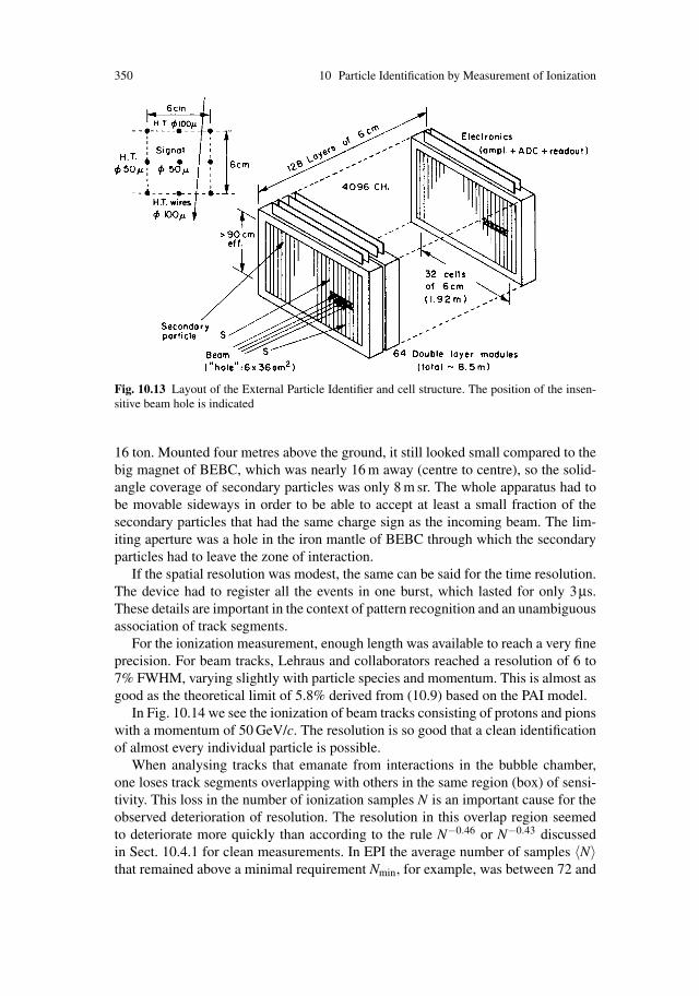
350 10 Particle Identification by Measurement of Ionization
Fig. 10.13 Layout of the External Particle Identifier and cell structure. The position of the insen-sitive beam hole is indicated
16 ton. Mounted four metres above the ground, it still looked small compared to thebig magnet of BEBC, which was nearly 16 m away (centre to centre), so the solid-angle coverage of secondary particles was only 8 m sr. The whole apparatus had tobe movable sideways in order to be able to accept at least a small fraction of thesecondary particles that had the same charge sign as the incoming beam. The lim-iting aperture was a hole in the iron mantle of BEBC through which the secondaryparticles had to leave the zone of interaction.
If the spatial resolution was modest, the same can be said for the time resolution.The device had to register all the events in one burst, which lasted for only 3μs.These details are important in the context of pattern recognition and an unambiguousassociation of track segments.
For the ionization measurement, enough length was available to reach a very fineprecision. For beam tracks, Lehraus and collaborators reached a resolution of 6 to7% FWHM, varying slightly with particle species and momentum. This is almost asgood as the theoretical limit of 5.8% derived from (10.9) based on the PAI model.
In Fig. 10.14 we see the ionization of beam tracks consisting of protons and pionswith a momentum of 50 GeV/c. The resolution is so good that a clean identificationof almost every individual particle is possible.
When analysing tracks that emanate from interactions in the bubble chamber,one loses track segments overlapping with others in the same region (box) of sensi-tivity. This loss in the number of ionization samples N is an important cause for theobserved deterioration of resolution. The resolution in this overlap region seemedto deteriorate more quickly than according to the rule N−0.46 or N−0.43 discussedin Sect. 10.4.1 for clean measurements. In EPI the average number of samples 〈N〉that remained above a minimal requirement Nmin, for example, was between 72 and

10.8 Performance Achieved in Existing Detectors 351
91 (momentum dependent), resulting in resolutions between 10.6 and 8.7%; seeTable 10.3.
Comparable in size was the large drift chamber ISIS2 (which stands for the ‘Iden-tification of Secondaries by Ionization Sampling’); it had a length of 5 m and anaperture of 2 m horizontally times 4 m vertically. A description is found in Chap. 11.Here we summarize its capabilities as an ionization-measuring device. With morefrequent and finer samplings than EPI, but with reduced length, it should have thesame resolving power, according to (10.9). Although the drift-time measurementallowed the vertical track coordinates in ISIS to be known to a few millimetres, thedetailed track filtering and subsequent hit association to tracks proved to be criti-cal for achieving a good resolution. For instance, in a typical study of secondarytracks in an experiment 10 m behind the small bubble chamber HOLEBC, the aver-age number of samples retainable per track was 〈N〉= 250, if the required minimumwas set to Nmin = 100. The achieved accuracy was 8.3% FWHM instead of the theo-retical 6.5% expected for this value of 〈N〉. Whereas such details depend entirely onthe track density in the chamber, they are quoted here to illustrate how the ionizationresolving power goes down with an increasing overlap of tracks.
With this apparatus the most probable ionization density of each track couldbe measured with an accuracy of 3.5% r.m.s. and the relativistic rise was 56%.Using the dependence of the ionization on the particle velocity, as well as themomenta determined in the spectrometer, useful particle identification was pos-sible up to 60 GeV. In order to give an impression of the achieved identificationreliability, we show in Fig. 10.15a,b the uniqueness f of the electron–pion sepa-ration as a function of particle momentum. The parameter f is defined to be thepercentage of correctly identified pions (probability > 1%) whose ionization is in-compatible with an electron at the 1% level, and this is equal to the percentageof correctly identified electrons incompatible with a pion. (These ratios could bemeasured because there was independent kinematical particle identification for asample of events.) Figure 10.15a,bb contains the same for the uniqueness of thepion–kaon separation.
Fig. 10.14 Distribution ofionization measured with EPIin an unseparated positivebeam line, 900 m downstreamof the target, at 50 GeV/cmomentum [LEH 78]

352 10 Particle Identification by Measurement of Ionization
Table 10.3 Wire chambers specialized in ionization measurement in fixed-target experiments
Chamber EPI ISIS2a CRISISExperiment Big European European Hybrid FNAL Hybrid
Bubble Chamber Spectrometer with Spectrometer withHOLEBC 30’ BC
Reference [LEH 78] [ALL 84] [TOO 88][BAR 83] [GOL 85]
Chamber typeb MWPC Stack type 3 drift chamber type 3 drift chamberMax. no. of samples per track 128 320 192Sample length (cm) 6 1.6 1.6Total length of sensitive 7.7 5.1 3.1volume (m)Size of entrance window 192×90 200×400 98×102hor. × vert. (cm)Max. drift length (cm) 6 200 25Gas mixture Ar(95)+CH4(5) Ar(80)+CO2(20) Ar(80)+CO2(20)Pressure (bar) 1 1 1Gas amplification factor 4000 10000 –Estimation method employedc 〈S〉40 M–L 〈S〉75
Analysis of beam tracks:Observed resolution 6.0–7.0 – 7.6–8.0(FWHM, per cent)Theoretical limit 5.8 5.8 7.4(our equation 9.9)
Analysis of secondary tracks:Min. no. of useful 50 80 100 50samples requiredAverage no. of useful (72–91)d (91–109)d 250 140e
samples obtainedObserved resolution (10.6–8.7) (8.7–7.8) 8.3 10(FWHM, per cent)Theoretical limit (7.6–7.8) (6.8–6.4) 6.5 8.7(our (9.9))
Relativistic rise 58 56 � 45(per cent over the minimum)
a Chamber also described in Sect. 11.7.5.b Drift chamber definitions, see Sect. 11.1.c Notation, see Sect. 10.3; M–L is maximum likelihood.d Depending on momenta of secondaries.e Our estimate.
The achieved degree of particle identification is also demonstrated in the scatterplot of momentum vs. ionization of Fig. 10.16. Working with secondary particlesof known masses and momenta, Allison and colleagues were able to compare theionization measurement with expectations based on the PAI model. In the plot wesee electrons, pions and protons, but no muons or kaons, because these were notin the sample of kinematically identified tracks; this simplified the situation. Onecan easily make out the regions in the drawing where the measured tracks are un-ambiguously associated to one line, i.e. identified. Some confusion between pions
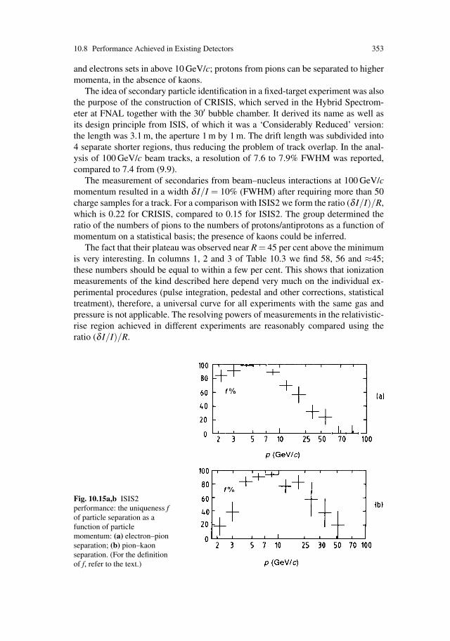
10.8 Performance Achieved in Existing Detectors 353
and electrons sets in above 10 GeV/c; protons from pions can be separated to highermomenta, in the absence of kaons.
The idea of secondary particle identification in a fixed-target experiment was alsothe purpose of the construction of CRISIS, which served in the Hybrid Spectrom-eter at FNAL together with the 30′ bubble chamber. It derived its name as well asits design principle from ISIS, of which it was a ‘Considerably Reduced’ version:the length was 3.1 m, the aperture 1 m by 1 m. The drift length was subdivided into4 separate shorter regions, thus reducing the problem of track overlap. In the anal-ysis of 100 GeV/c beam tracks, a resolution of 7.6 to 7.9% FWHM was reported,compared to 7.4 from (9.9).
The measurement of secondaries from beam–nucleus interactions at 100 GeV/cmomentum resulted in a width δ I/I = 10% (FWHM) after requiring more than 50charge samples for a track. For a comparison with ISIS2 we form the ratio (δ I/I)/R,which is 0.22 for CRISIS, compared to 0.15 for ISIS2. The group determined theratio of the numbers of pions to the numbers of protons/antiprotons as a function ofmomentum on a statistical basis; the presence of kaons could be inferred.
The fact that their plateau was observed near R = 45 per cent above the minimumis very interesting. In columns 1, 2 and 3 of Table 10.3 we find 58, 56 and ≈45;these numbers should be equal to within a few per cent. This shows that ionizationmeasurements of the kind described here depend very much on the individual ex-perimental procedures (pulse integration, pedestal and other corrections, statisticaltreatment), therefore, a universal curve for all experiments with the same gas andpressure is not applicable. The resolving powers of measurements in the relativistic-rise region achieved in different experiments are reasonably compared using theratio (δ I/I)/R.
Fig. 10.15a,b ISIS2performance: the uniqueness fof particle separation as afunction of particlemomentum: (a) electron–pionseparation; (b) pion–kaonseparation. (For the definitionof f, refer to the text.)
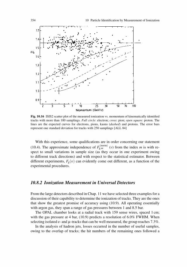
354 10 Particle Identification by Measurement of Ionization
Fig. 10.16 ISIS2 scatter plot of the measured ionization vs. momentum of kinematically identifiedtracks with more than 100 samplings. Full circle: electron; cross: pion; open square: proton. Thelines are the expected curves for electrons, pions, kaons (dashed) and protons. The error barsrepresent one standard deviation for tracks with 250 samplings [ALL 84]
With this experience, some qualifications are in order concerning our statement
(10.4). The approximate independence of F(norm)g,m (v) from the index m is with re-
spect to small variations in sample size (as they occur in one experiment owingto different track directions) and with respect to the statistical estimator. Betweendifferent experiments, Fg(v) can evidently come out different, as a function of theexperimental procedures.
10.8.2 Ionization Measurement in Universal Detectors
From the large detectors described in Chap. 11 we have selected three examples for adiscussion of their capability to determine the ionization of tracks. They are the onesthat show the greatest promise of accuracy using (10.9). All operating essentiallywith argon gas, they span a range of gas pressures between 1 and 8.5 bar.
The OPAL chamber looks at a radial track with 159 sense wires, spaced 1 cm;with the gas pressure at 4 bar, (10.9) predicts a resolution of 6.0% FWHM. Whenselecting isolated e- and μ-tracks that can be well measured, the group reaches 7.3%.
In the analysis of hadron jets, losses occurred in the number of useful samples,owing to the overlap of tracks; the hit numbers of the remaining ones followed a

10.8 Performance Achieved in Existing Detectors 355
Fig. 10.17 OPAL study ofthe dependence of theresolution δ I/I (r.m.s.) on thenumber of ionization samplesN used per track. Uppercurve: Minimally ionizingpions within jets. Lowercurve: Single μ and e tracks(number of good ionizationsamples artificially reduced)[HAU 91]
distribution between 0 and 159, peaking at 110 with 89% above 40. On average,well-measured tracks had 94 samples, and a resolution of 8.9% FWHM was ob-tained. Equation (10.9) predicts 7.6% for these. Again, the deterioration is worsethan would be expected from the reduced number of samples alone.
The OPAL group has made a special study of this effect by plotting in Fig. 10.17the accuracy reached within jets for minimally ionizing pions as a function of thenumber of useful samples. This is compared with data for isolated particles. Thesedata contain usually the (almost) full number of wires, and these are then artifi-cially reduced by randomly removing good signals; the remaining number N ofsamples was found to determine the accuracy proportional to N−0.43. The curvefor particles in jets is worse than (i.e. lies above) the one for isolated particles, forevery N. We may suspect that problems of space charge near the wires and in thedrift region as well as residual problems of pattern recognition are the cause of thisbehaviour.
The PEP-4 TPC can measure a good track 183 times. With the wires spacedat x = 0.4 cm and the gas pressure 8.5 bar, the individual sample length px is verysimilar to that of the OPAL chamber. On the basis of (10.9), one expects a resolutionof 5.9% FWHM, and 6.9% is reached for isolated tracks.
The tracks in particle jets are measured with a resolution of 8.3% FWHM. Thenumber of lost samples is our own estimate; as in the case of OPAL, it does not fullyaccount for the reduction in accuracy, compared to the isolated tracks.
The ALEPH TPC is almost twice as large in radius as the PEP-4 TPC and canmeasure radial tracks on 340 wires. Operating with atmospheric gas pressure, itsindividual sample length is only px = 0.4 cm bar, smaller than in any other driftchamber. The signals are therefore extremely feeble. In the minimum of ionization,only eleven clusters contribute on average to the signal of a wire (cf. Table 1.1).According to (10.9), a resolution of 8.8% FWHM should be expected, and 10.3%has been reached for isolated tracks.

356 10 Particle Identification by Measurement of Ionization
Fig. 10.18 Scatter diagram ofionization strength versusparticle momentum formultihadronic and dimuonevents in Z0 decays, asmeasured with the OPAL JetChamber [HAU 91]
When studying tracks inside jets and of lower momenta, the large magnetic field(1.5 T; see Table 11.4) poses a special problem: particle tracks below 0.5 GeV/ccoil up inside the chamber and require angular corrections (cf. Sect. 10.7.2) overa large range of angles. The resolution for hadron tracks is 13.3% FWHM at theaverage value of N = 250 samples; this can be compared to the 10.2% expectedfrom (10.9).
Fig. 10.19 R.m.s.particle-separation power Das defined in the text,achieved with the OPAL JetChamber [HAU 91]

10.8 Performance Achieved in Existing Detectors 357
Table 10.4 Ionization-measuring capability of some universal drift chambers in colliderexperimentsa
Drift chamber OPAL Jet Chamber PEP 4 TPC ALEPH TPCReference [BRE 87] [COW 88] [ATW 91]
[HAU 91]Drift chamber typeb 2 3 3Max. no. of samples per track 159 183 340Sample length (cm bar) 4 3.4 0.4Max. drift length (cm) 3–25 100 220Gas mixture Ar(88)+CH4(10) Ar(80)+CH4(20) Ar(91)+CH4(9)
+ i-C4H10(2)Pressure (bar) 4 8.5 1Gas amplification factor 10000 – 5000Estimation method employedc 〈S〉70. 〈S〉65 〈S〉60
Analysis of isolated tracks:Min. polar angle required (deg): 45 45 45Observed resolution 7.3 6.9 10.3(FWHM, per cent)Theoretical limitd 6.0 5.9 8.8(our (10.9))
Analysis of tracks inside jets:Min. polar angle required (deg): 45 45 45Min. no. of usefulsamples required 40 80 150Average no. of usefulsamples obtained 94 140f 250Observed resolutione
(FWHM, per cent) 8.9 8.3 ± 0.7 13.3Theoretical limitg
(our (10.9)) 7.6 6.7 10.2
Relativistic rise observed(per cent over the minimum) 47 37 57Measured resolution for isolatedtracks (FWHM), divided by theobserved relativistic rise 0.155 0.186 0.181
aMore details on these chambers can be found in Tables 11.2 and 11.4bDefinitions Sect. 11.1cDefinitions Sect. 10.3dUsing lines 4 and 5 above (the effects of slightly larger average sample size and any loss ofsamples are neglected)ePions in the minimum of ionizationfOur estimategUsing lines 5 and 16 above
In a comparison of these three detectors one must consider the different gas pres-sures. The relativistic rise R, expressed as the percentage difference of the plateauover the minimum, is better for the smaller pressures. On the other hand, the res-olution δ I/I is better for the higher pressures. A useful over-all criterion is the
358 10 Particle Identification by Measurement of Ionization
measured ratio δ I/(IR), which we have computed in the last line of Table 10.4.The best figure of merit belongs to the OPAL Jet Chamber; for it we show thescatter diagram of ionization strength versus particle momentum in Fig. 10.18. TheOPAL r.m.s. particle-separation power D for various pairs of particles is plotted inFig. 10.19 as a function of momentum. The quantity D12 is defined as the ratio ofthe difference of the ionization strengths of the two particles 1 and 2 to the averageresolution
D12 =|I1 − I2|
(δ I1/I1 +δ I2/I2)/2.
Experimentally, the two terms in the denominator are equal.
References
[ALL 80] W.W.M. Allison, Relativistic charged particle identification by energy-loss, Ann.Rev. Nucl. Sc. 30, 253 (1980)
[ALL 82] W.W.M. Allison, Relativistic particle identification by dE/dx: the fruits of experi-ence with ISIS, in Int. Conf. for Colliding Beam Physics, SLAC, 61 (1982)
[ALL 84] W.W.M. Allison, C.B. Brooks, P.D. Shield, M. Aguilar Benitez, C. Willmot,J. Dumarchez and M. Schouten, Relativistic charged particle identification withISIS2, Nucl. Instrum. Methods Phys. Res. 224, 396 (1984)
[ASS 90] R. Assmann, Ionisationsmessung und Teilchenidentifizierung in der zentralenSpurendriftkammer (TPC) von ALEPH, Diploma Thesis University of Munich1990, unpublished
[ASS 91] We thank R. Assmann (Munich) for the computation of the fits[ATW 91] W.B. Atwood et al., Performance of the ALEPH time projection chamber, Nucl.
Instrum. Methods Phys. Res. A 306, 446 (1991)[BAR 83] V. Baruzzi et al., Use of a large multicell ionization detector – the External Particle
Identifier – in experiments with the BEBC hydrogen bubble chamber, Nucl. Instrum.Methods 207, 339 (1983)
[BLU 74] W. Blum, K. Sochting, U. Stierlin, Gas Phenomena in spark chambers, Phys. Rev. A10, 491 (1974)
[BRE 87] H. Breuker et al., Particle identification with the OPAL jet chamber in the region ofthe relativistic rise, Nucl. Instrum. Methods Phys. Res. A 260, 329 (1987)
[COW 88] G.D. Cowan, Inclusive π , K and p, p− production in e+e− annihilation at√
s =29 GeV, Dissertation, University of California, Berkeley (1988), also Berkeleypreprint LBL-24715
[CRA 51] H. Cramer, Mathematical Methods of Statistics (Princeton University Press 1951)[DAV 69] V.A. Davidenko, B.A. Dolgoshein, V.K. Semenov, S.V. Somov, Measurements of
the relativistic increase of the specific primary ionization in a streamer chamber,Nucl. Instrum. Methods 67, 325 (1969)
[EAD 71] W.T. Eadie, D. Dryard, F.E. James, M. Roos, B. Sadoulet, Statistical Methods inExperimental Physics (North-Holland, Amsterdam 1971)
[ERM 77] V.C. Ermilova, L.P. Kotenko and G.I. Merzon, Fluctuations and the most probablevalues of relativistic charged particle energy loss in thin gas layers, Nucl. Instrum.Methods 145, 555 (1977)
[FIS 58] M. Fisz, Wahrscheinlichkeitsrechnung und mathematische Statistik (translated fromPolish) (VEB Verlag der Wissenschaften, Berlin 111989)
[GOL 85] D. Goloskie, V. Kistiakowsky, S. Oh, I.A. Pless, T. Stroughton, V. Suchorebrow,B. Wadsworth, O. Murphy, R. Steiner and H.D. Taft, The performance of CRISISand its calibration, Nucl. Instrum. Methods Phys. Res. A 238, 61 (1985)
References 359
[HAU 91] M. Hauschild et al., Particle identification with the OPAL Jet Chamber, CERNpreprint PPE/91-130 (August 1991), to appear in Nucl. Instrum. Methods Phys. Res.
[LEH 78] I. Lehraus, R. Matthewson, W. Tejessy and M. Aderholz, Performance of alargescale multilayer ionization detector and its use for measurements of the rel-ativistic rise in the momentum range of 20–110 GeV/c, Nucl. Instrum. Methods 153,347 (1978)
[LEH 82a] I. Lehraus, R. Mathewson and W. Tejessi, Particle identification by dE/dx samplingin high pressure drift detectors, Nucl. Instrum. Methods 196, 361 (1982)
[LEH 82b] I. Lehraus, R. Mathewson and W. Tejessi, dE/dx measurements in Ne, Ar, Kr, Xeand pure hydrocarbons, Nucl. Instrum. Methods 200, 199 (1982)
[TOO 88] W.S. Toothackier et al., Secondary particle identification using the relativistic rise inionization, Nucl. Instrum. Methods Phys. Res. A 273, 97 (1988)
[WAL 79a] A.H. Walenta, J. Fischer, H. Okuno and C.L. Wang, Measurement of the ionizationloss in the region of relativistic rise for noble and molecular gases, Nucl. Instrum.Methods 161, 45 (1979)
[WAL 79b] A.H. Walenta, The time expansion chamber and single ionization cluster measure-ment, IEEE Trans. Nucl. Sc. NS-26, 73 (1979)


Chapter 11Existing Drift Chambers – An Overview
Drift chambers have in common that the drift of the ionization electrons in the gas isused for a coordinate determination by measurement of the drift time. In this chapterwe want to take a look at the large variety of forms in which drift chambers havebeen built for particle physics. As a complete coverage of all existing drift chambersdoes not correspond to our plan we subdivide the material according to a geometricalcriterion into three basic types, and then we discuss typical forms within each type.The selection of chambers is intended to represent the different choices that havebeen made in this field, but a certain arbitrariness in choosing the examples wasunavoidable. Of the chambers we know, we have preferred those that are alreadyworking to similar ones that are still in a state of preparation; and those that are welldocumented we have preferred to similar ones with less detailed descriptions. Wehave considered drift chambers for the detection of charged particles, but not thosefor single photons, so the image chambers useful in biology and medicine have beenleft out as well as those used to detect Cerenkov radiation.
A description of drift chambers in the context of particle-physics experiments isgiven in the review article by Williams [WIL 86].
Let us begin by defining the three basic types.
11.1 Definition of Three Geometrical Types of Drift Chambers
Type 1: The simplest drift chamber is ideally a sensitive area placed across thepath of a particle in order to measure one, or perhaps both, coordinates of thepoint of penetration. It was developed out of the multiwire proportional chamber,or MWPC – a hodoscope of parallel proportional wires – by supplementing theelectronics of the sense wires with equipment to measure the time of the avalanchepulse and hence the drift time of the ionization electrons. The electric field in thedrift region is shaped, usually with conductors on defined potentials like field wires,but sometimes also by charges deposited on insulators.
In practice, the ionization electrons of a short piece of track are collected on thenearest sense wire. For a complete determination of track parameters, such chambers
W. Blum et al., Particle Detection with Drift Chambers, 361doi: 10.1007/978-3-540-76684-1 11, c© Springer-Verlag Berlin Heidelberg 2008
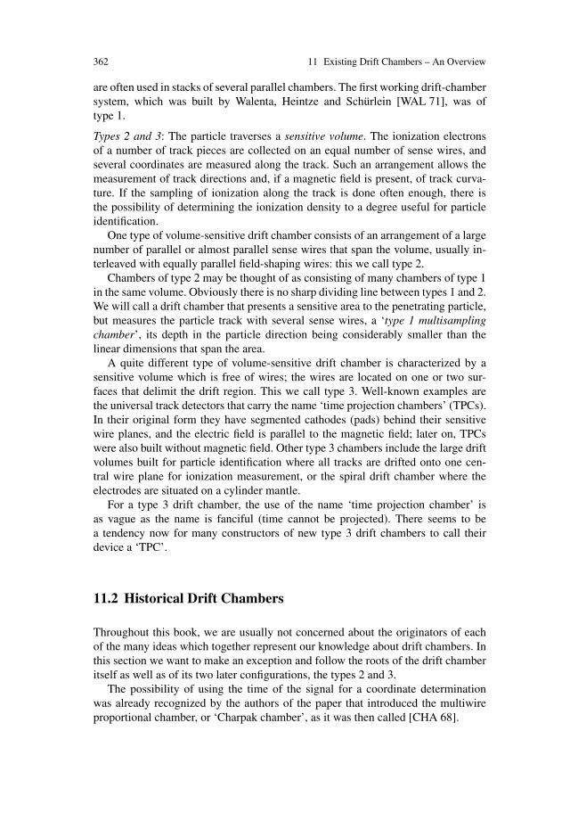
362 11 Existing Drift Chambers – An Overview
are often used in stacks of several parallel chambers. The first working drift-chambersystem, which was built by Walenta, Heintze and Schurlein [WAL 71], was oftype 1.
Types 2 and 3: The particle traverses a sensitive volume. The ionization electronsof a number of track pieces are collected on an equal number of sense wires, andseveral coordinates are measured along the track. Such an arrangement allows themeasurement of track directions and, if a magnetic field is present, of track curva-ture. If the sampling of ionization along the track is done often enough, there isthe possibility of determining the ionization density to a degree useful for particleidentification.
One type of volume-sensitive drift chamber consists of an arrangement of a largenumber of parallel or almost parallel sense wires that span the volume, usually in-terleaved with equally parallel field-shaping wires: this we call type 2.
Chambers of type 2 may be thought of as consisting of many chambers of type 1in the same volume. Obviously there is no sharp dividing line between types 1 and 2.We will call a drift chamber that presents a sensitive area to the penetrating particle,but measures the particle track with several sense wires, a ‘type 1 multisamplingchamber’, its depth in the particle direction being considerably smaller than thelinear dimensions that span the area.
A quite different type of volume-sensitive drift chamber is characterized by asensitive volume which is free of wires; the wires are located on one or two sur-faces that delimit the drift region. This we call type 3. Well-known examples arethe universal track detectors that carry the name ‘time projection chambers’ (TPCs).In their original form they have segmented cathodes (pads) behind their sensitivewire planes, and the electric field is parallel to the magnetic field; later on, TPCswere also built without magnetic field. Other type 3 chambers include the large driftvolumes built for particle identification where all tracks are drifted onto one cen-tral wire plane for ionization measurement, or the spiral drift chamber where theelectrodes are situated on a cylinder mantle.
For a type 3 drift chamber, the use of the name ‘time projection chamber’ isas vague as the name is fanciful (time cannot be projected). There seems to bea tendency now for many constructors of new type 3 drift chambers to call theirdevice a ‘TPC’.
11.2 Historical Drift Chambers
Throughout this book, we are usually not concerned about the originators of eachof the many ideas which together represent our knowledge about drift chambers. Inthis section we want to make an exception and follow the roots of the drift chamberitself as well as of its two later configurations, the types 2 and 3.
The possibility of using the time of the signal for a coordinate determinationwas already recognized by the authors of the paper that introduced the multiwireproportional chamber, or ‘Charpak chamber’, as it was then called [CHA 68].
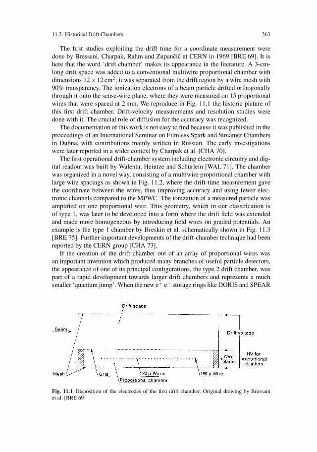
11.2 Historical Drift Chambers 363
The first studies exploiting the drift time for a coordinate measurement weredone by Bressani, Charpak, Rahm and Zupancic at CERN in 1969 [BRE 69]. It ishere that the word ‘drift chamber’ makes its appearance in the literature. A 3-cm-long drift space was added to a conventional multiwire proportional chamber withdimensions 12×12 cm2; it was separated from the drift region by a wire mesh with90% transparency. The ionization electrons of a beam particle drifted orthogonallythrough it onto the sense-wire plane, where they were measured on 15 proportionalwires that were spaced at 2 mm. We reproduce in Fig. 11.1 the historic picture ofthis first drift chamber. Drift-velocity measurements and resolution studies weredone with it. The crucial role of diffusion for the accuracy was recognized.
The documentation of this work is not easy to find because it was published in theproceedings of an International Seminar on Filmless Spark and Streamer Chambersin Dubna, with contributions mainly written in Russian. The early investigationswere later reported in a wider context by Charpak et al. [CHA 70].
The first operational drift-chamber system including electronic circuitry and dig-ital readout was built by Walenta, Heintze and Schurlein [WAL 71]. The chamberwas organized in a novel way, consisting of a multiwire proportional chamber withlarge wire spacings as shown in Fig. 11.2, where the drift-time measurement gavethe coordinate between the wires, thus improving accuracy and using fewer elec-tronic channels compared to the MPWC. The ionization of a measured particle wasamplified on one proportional wire. This geometry, which in our classification isof type 1, was later to be developed into a form where the drift field was extendedand made more homogeneous by introducing field wires on graded potentials. Anexample is the type 1 chamber by Breskin et al. schematically shown in Fig. 11.3[BRE 75]. Further important developments of the drift-chamber technique had beenreported by the CERN group [CHA 73].
If the creation of the drift chamber out of an array of proportional wires wasan important invention which produced many branches of useful particle detectors,the appearance of one of its principal configurations, the type 2 drift chamber, waspart of a rapid development towards larger drift chambers and represents a muchsmaller ‘quantum jump’. When the new e+ e− storage rings like DORIS and SPEAR
Fig. 11.1 Disposition of the electrodes of the first drift chamber. Original drawing by Bressaniet al. [BRE 69]

364 11 Existing Drift Chambers – An Overview
Fig. 11.2 Disposition of the electrodes in the chamber built by Walenta et al.
required particle tracking in all directions around the interaction point, the most ob-vious design was the one where several cylindrical type 1 chambers with increasingdiameters were inserted into one another, each one an entity that could be pulledout for maintenance. The MARK I drift chambers and the PLUTO spark chamberswere examples of this geometry.
The first genuine type 2 drift chamber was that of the old MARK II detector atSPEAR [DAV 79]. Its designers had taken the essential step of filling the entire sen-sitive volume with wires strung between two opposite end-plates, having done awaywith all intermediate ring-shaped structures and gas foils, thus paving the way for anew generation of larger volume-sensitive drift chambers of very high accuracy. Adescription of the state of the art in 1981 may be found in [WAG 81] and [FLU 81].
The origin of the type 3 drift chambers is in Oxford. The ISIS project for theIdentification of Secondaries by Ionization Sampling was first described in 1973[MUL 73, ALL 74], and a prototype with an 85-cm-long drift was tested the sameyear [see ALL 82]. The basic idea was a large sensitive volume that contained onlygas and an electric field, the track ionization being collected and measured on asingle wire plane. Multihit electronics recorded the drift times of all the tracks ofone event, thus producing a direct image of the event in one projection. The purposeof the apparatus was not primarily a precise determination of coordinates (for thisthe diffusion was too large as a consequence of the long drift) but the measurementof ionization density for particle identification. A later version of ISIS is describedin Sects. 11.7 and 10.7. ISIS can be considered a predecessor of the TPC.
Fig. 11.3 Disposition of the electrodes in the chamber built by Breskin et al. [BRE 75], cathodewires at uniformly decreasing potentials produce a long and homogeneous drift field
11.3 Drift Chambers for Fixed-Target and Collider Experiments 365
The first time the TPC concept appeared on paper was in a laboratory report byD. Nygren [NYG 74]. The chamber was subsequently built at Berkeley and SLACfor the PEP-4 experiment. Again, it is not easy to find access to a documentationof this work. A very detailed description of the PEP-4 TPC is contained in theexperiment proposal of the collaborating institutes [CLA 76]. It was presented tothe appropriate bodies for approval and later widely circulated among workers in thefield. This proposal and its numerous appendices reported on many aspects of thefeasibility of a TPC. Some of this important material has never been published.
Conscious [NYG 83] of the latest work at CERN and at Oxford, Nygren inventedthe TPC by performing a synthesis into one instrument of all the known elements:long drift, diffusion suppression through parallel E and B fields, 3-dimensional co-ordinate measurement by pick-up electrodes for x and y, and drift-time measurementfor z. This was made possible by a novel storage of the pulse train of every electrodeover the full length of the drift time. The PEP-4-TPC is described in more detail inSect. 11.7.
11.3 Drift Chambers for Fixed-Targetand Collider Experiments
A typical fixed-target experiment would have an arrangement of type 1 chambersthat record (together with other detectors) the reaction products behind a target. Ifin addition to their directions one also measures the momenta of these particles withthe help of a magnet, then we have a magnetic spectrometer, a typical form of whichis schematically drawn in Fig. 11.4. Stacks of planar type 1 chambers have been inwide use for such spectrometers.
As for the momentum-measuring accuracy δ p/p at a given bending power pB ofthe magnet, the contribution of each arm is, in a first approximation, proportional toδx/L, the ratio of the chamber point-measuring accuracy to the length of the leverarm (or thickness of the stack):
δ pp
= constp
pB
δxL
.
Fig. 11.4 A typical magnetspectrometer behind a fixedtarget T, using stacks of type1 drift chambers (DCs) infront of and behind themagnet M
366 11 Existing Drift Chambers – An Overview
Often there is freedom to increase L; then the value of δx is less critical, but thedimensions W of the chambers must be increased in proportion.
For the study of very-high-multiplicity events in heavy-ion fixed-target experi-ments, even type 3 chambers have become popular. The direct three-dimensionalmeasurement of track elements is an advantage for such events (see Sect. 11.7).
An important group of drift chambers has been built around the interaction re-gions of particle colliders where they are – together with the installed calorimeters –the principal instruments for the investigation of the particles from the collisions.Close to the interaction point we find the vertex detectors around the beam pipewhose purpose it is to determine the interaction vertex with high precision. Fur-ther out in radius the main drift chambers measure the direction and momenta of thecharged particles and, in many cases, their ionization. In the design of these trackingdevices the choice of the magnetic field and its orientation is a primary concern.
11.3.1 General Considerations Concerning the Directions of Wiresand Magnetic Fields
For symmetric electron–positron machines where one studies point-like interac-tion – these cause essentially isotropic particle distributions – the magnetic fieldB was most naturally created by a solenoid on axis with the particle beams. A goodmeasurement of particle momenta requires the curvature of tracks to be determinedwith the greatest accuracy in the azimuthal direction. In drift chambers of type 2it is the drift-time measurement that provides the accuracy; hence the wires are es-sentially parallel to the magnetic field (‘axial wire chambers’). In drift chambers oftype 3 the azimuthal accuracy is provided by cathode pick-up electrodes so that theelectric drift field can be made parallel to B. Therefore, in e+ e− machines we findaxial wire chambers and TPC’s along the direction of the beams. Along B, particlecurvature is not measurable.
For the study of hadron interactions in the pp and pp colliders, the magnetic fieldB has sometimes been chosen to be at right angles to the beam direction, on accountof the important flux of high-momentum particles in the direction of the beams – theUAI-experiment at the CERN pp collider and the Split Field Magnet at the CERNIntersecting Storage Rings being well-known examples. The orientation of the wiresof type 1 or type 2 drift chambers again has to be parallel to B, which is also theflight direction of the particles with vanishing curvature.
At the e− p collider HERA at DESY there is an inherent asymmetry in the en-ergies of the colliding particles, because 30 GeV electrons collide with 800 GeVprotons. The solution adopted for each of the two experiments is a solenoid, coaxialwith the beams, instrumented with a coaxial type 2 chamber, and complemented inthe forward direction of high momenta with several planar type 1 stacks for particleswith polar angles θ approximately between 10 and 30◦. In these type 1 chamberswe find the sense wires orthogonal to the magnetic field, thus giving an accuratemeasurement of θ and a good double track resolution in this angular range.

11.3 Drift Chambers for Fixed-Target and Collider Experiments 367
11.3.2 The Dilemma of the Lorentz Angle
In drift chambers of type 2, for an accurate determination of the curvature of anionization track one compares the times of arrival of the electrons from differenttrack segments on different wires (Fig. 11.5a-ca). The best accuracy is obtainedwhen the electron drift is at right angles to the track; for then the time differencesmeasure the curvature directly, and also the electrons of every track segment thatgo to the same sense wire are most concentrated in arrival times and hence give thesmallest variance in the measurement (cf. Sect. 7.3).
However, the magnetic field B orthogonal to the electric drift field E forces theelectrons towards the direction given by the vector product – [E × B]. The Lorentzangle ψ between the drift direction u and E, in the approximation of Sects. 2.1and 2.2 (2.1.1) is given by
tanψ = ωτ .
Figure 11.5a-cb shows the resulting disadvantage: not only does one have tomeasure the sagitta under an angle of projection, but also inside every track segmentthe arrival times are spread out more than before. This gives rise to the ‘angularwire term’ in (7.26), with α = ψ , even if the track is perfectly radial. Therefore,in this geometry one is obliged to keep ωτ small, although – in the interest of agood momentum measurement – one wants the largest possible B field. This is thedilemma of the Lorentz angle.
Since τ is related to the electron mobility μ by the approximate relationμ = (e/m)τ (for more details see Chap. 2), one way out of the dilemma is to choose a
Fig. 11.5a-c Drift paths of ionization electrons from the particle track to the sense wires. (a)ωτ = 0 (no magnetic field); (b) ωτ = 1, sense wire plane parallel to the tack; (c) ωτ = 1, sense-wire plane inclined
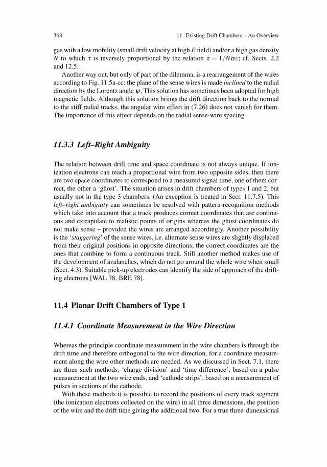
368 11 Existing Drift Chambers – An Overview
gas with a low mobility (small drift velocity at high E field) and/or a high gas densityN to which τ is inversely proportional by the relation τ = 1/Nσc; cf. Sects. 2.2and 12.5.
Another way out, but only of part of the dilemma, is a rearrangement of the wiresaccording to Fig. 11.5a-cc: the plane of the sense wires is made inclined to the radialdirection by the Lorentz angle ψ . This solution has sometimes been adopted for highmagnetic fields. Although this solution brings the drift direction back to the normalto the stiff radial tracks, the angular wire effect in (7.26) does not vanish for them.The importance of this effect depends on the radial sense-wire spacing.
11.3.3 Left–Right Ambiguity
The relation between drift time and space coordinate is not always unique. If ion-ization electrons can reach a proportional wire from two opposite sides, then thereare two space coordinates to correspond to a measured signal time, one of them cor-rect, the other a ‘ghost’. The situation arises in drift chambers of types 1 and 2, butusually not in the type 3 chambers. (An exception is treated in Sect. 11.7.5). Thisleft–right ambiguity can sometimes be resolved with pattern-recognition methodswhich take into account that a track produces correct coordinates that are continu-ous and extrapolate to realistic points of origins whereas the ghost coordinates donot make sense – provided the wires are arranged accordingly. Another possibilityis the ‘staggering’ of the sense wires, i.e. alternate sense wires are slightly displacedfrom their original positions in opposite directions; the correct coordinates are theones that combine to form a continuous track. Still another method makes use ofthe development of avalanches, which do not go around the whole wire when small(Sect. 4.3). Suitable pick-up electrodes can identify the side of approach of the drift-ing electrons [WAL 78, BRE 78].
11.4 Planar Drift Chambers of Type 1
11.4.1 Coordinate Measurement in the Wire Direction
Whereas the principle coordinate measurement in the wire chambers is through thedrift time and therefore orthogonal to the wire direction, for a coordinate measure-ment along the wire other methods are needed. As we discussed in Sect. 7.1, thereare three such methods: ‘charge division’ and ‘time difference’, based on a pulsemeasurement at the two wire ends, and ‘cathode strips’, based on a measurement ofpulses in sections of the cathode.
With these methods it is possible to record the positions of every track segment(the ionization electrons collected on the wire) in all three dimensions, the positionof the wire and the drift time giving the additional two. For a true three-dimensional
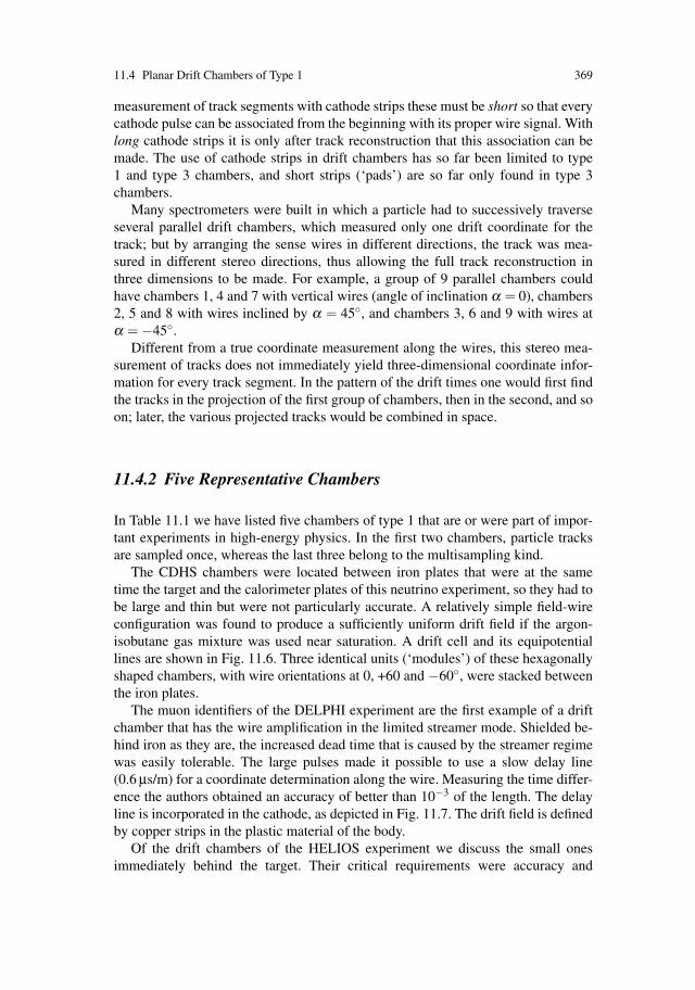
11.4 Planar Drift Chambers of Type 1 369
measurement of track segments with cathode strips these must be short so that everycathode pulse can be associated from the beginning with its proper wire signal. Withlong cathode strips it is only after track reconstruction that this association can bemade. The use of cathode strips in drift chambers has so far been limited to type1 and type 3 chambers, and short strips (‘pads’) are so far only found in type 3chambers.
Many spectrometers were built in which a particle had to successively traverseseveral parallel drift chambers, which measured only one drift coordinate for thetrack; but by arranging the sense wires in different directions, the track was mea-sured in different stereo directions, thus allowing the full track reconstruction inthree dimensions to be made. For example, a group of 9 parallel chambers couldhave chambers 1, 4 and 7 with vertical wires (angle of inclination α = 0), chambers2, 5 and 8 with wires inclined by α = 45◦, and chambers 3, 6 and 9 with wires atα = −45◦.
Different from a true coordinate measurement along the wires, this stereo mea-surement of tracks does not immediately yield three-dimensional coordinate infor-mation for every track segment. In the pattern of the drift times one would first findthe tracks in the projection of the first group of chambers, then in the second, and soon; later, the various projected tracks would be combined in space.
11.4.2 Five Representative Chambers
In Table 11.1 we have listed five chambers of type 1 that are or were part of impor-tant experiments in high-energy physics. In the first two chambers, particle tracksare sampled once, whereas the last three belong to the multisampling kind.
The CDHS chambers were located between iron plates that were at the sametime the target and the calorimeter plates of this neutrino experiment, so they had tobe large and thin but were not particularly accurate. A relatively simple field-wireconfiguration was found to produce a sufficiently uniform drift field if the argon-isobutane gas mixture was used near saturation. A drift cell and its equipotentiallines are shown in Fig. 11.6. Three identical units (‘modules’) of these hexagonallyshaped chambers, with wire orientations at 0, +60 and −60◦, were stacked betweenthe iron plates.
The muon identifiers of the DELPHI experiment are the first example of a driftchamber that has the wire amplification in the limited streamer mode. Shielded be-hind iron as they are, the increased dead time that is caused by the streamer regimewas easily tolerable. The large pulses made it possible to use a slow delay line(0.6 μs/m) for a coordinate determination along the wire. Measuring the time differ-ence the authors obtained an accuracy of better than 10−3 of the length. The delayline is incorporated in the cathode, as depicted in Fig. 11.7. The drift field is definedby copper strips in the plastic material of the body.
Of the drift chambers of the HELIOS experiment we discuss the small onesimmediately behind the target. Their critical requirements were accuracy and

370 11 Existing Drift Chambers – An Overview
Tabl
e11
.1So
me
plan
ardr
iftc
ham
bers
ofty
pe1
Nam
eof
expe
rim
ent
CD
HS
DE
LPH
IN
A34
/HE
LiO
SL
3H
1N
ame
ofch
ambe
rD
CM
uon
Iden
tifier
DC
1M
iddl
eM
uon
Cha
mbe
rFT
D(r
adia
lwir
es)
Am
plifi
catio
nm
ode
Prop
ortio
nal
Lim
ited-
stre
amer
Prop
ortio
nal
Prop
ortio
nal
Prop
ortio
nal
Met
hod
ofz-
mea
sure
men
tSt
ereo
(suc
cess
ive
Tim
edi
ffer
ence
Ster
eo(s
ucce
ssiv
eSp
ecia
lcha
mbe
rC
harg
edi
visi
onm
odul
es)
(del
aylin
e)m
odul
es)
(alo
ngr)
Ref
eren
ce[M
AR
77]
[DA
U86
][B
ET
86]
[AD
E90
][B
EC
89]
[FA
B90
][G
RA
89]
Geo
met
ry
Wid
th(c
m)×
leng
th(c
m)
(one
cham
ber)
400×
400
(hex
agon
al)
20×
435
24(d
iam
)16
3×
556
30(i
nner
diam
)15
2(o
uter
diam
)To
tala
rea
ofth
ese
cham
bers
inex
peri
men
t(m
2)
720
600
0.4
280
5
No.
ofse
nse
wir
espe
rce
ll1
18
2412
No.
ofce
llspe
rch
ambe
r13
01
816
48Se
nse-
wir
esp
acin
g(m
m)
alon
gth
etr
ack
––
6(2
)9
10
Sens
e-w
ire
diam
eter
(μm
)40
100
2030
50M
ax.d
rift
leng
th(c
m)
310
1.5
51–
5(p
ropo
rtio
nal
tor)
Gap
(mm
)30
2048
360
120

11.4 Planar Drift Chambers of Type 1 371
Tabl
e11
.1(c
ontin
ued)
Gas
and
field
s
Gas
(per
cent
age
conc
entr
atio
n)A
r(70
)A
r(14
)+C
O2(7
0)C
O2(9
0)A
r(62
)X
e(30
)+
i-C
4H
10(3
0)+
i-C
4H
10(1
4)+
C2
H6(1
0)+
C2H
6(3
8)+
C2H
6(4
0)+
iso-
prop
yl-a
lcoh
ol(2
)+
He(
30)
Ele
ctri
cdr
iftfi
eld
(kV
/cm
)≥
10.
71.
21.
11.
2M
agne
ticfie
ld(T
)0
00
0.51
1.2
Dri
ftve
loci
ty(c
m/μ
s)5.
00.
751.
04.
93
Perf
orm
ance
(1)
Poin
t-m
easu
ring
accu
racy
per
wir
eIn
drif
tdir
ectio
nσ x
(mm
)<
0.7
(c)
1(b
)0.
12(c
)0.
17(c
)(3
)0.
11–0
.15
(b)
0.06
(b)
Inw
ire
dire
ctio
nσ z
(mm
)–
3(b
)–
–20
(b)
Dou
ble
trac
kre
solu
tion
Δ(m
m)
30(a
)10
0.6
(b)
Not
know
nA
ppro
x.1.
5(b
)1.
0(c
)
1.T
hepe
rfor
man
cefig
ures
are
base
don
(a)
calc
ulat
ion
and
labo
rato
ryte
sts;
(b)
prot
otyp
ean
dte
st-b
eam
mea
sure
men
ts;
(c)
mea
sure
men
tsin
the
runn
ing
expe
rim
ent.
2.C
harg
eco
llect
ion
per
sens
ew
ire:
2.5–
3m
min
trac
kdi
rect
ion.
3.T
his
led
toa
mom
entu
mre
solu
tion
mea
sure
din
the
expe
rim
ente
qual
toδ
p t/
p2 t=
5.3×
10−
4(G
eV/c
)−1
for
high
mom
entu
mm
uons
.
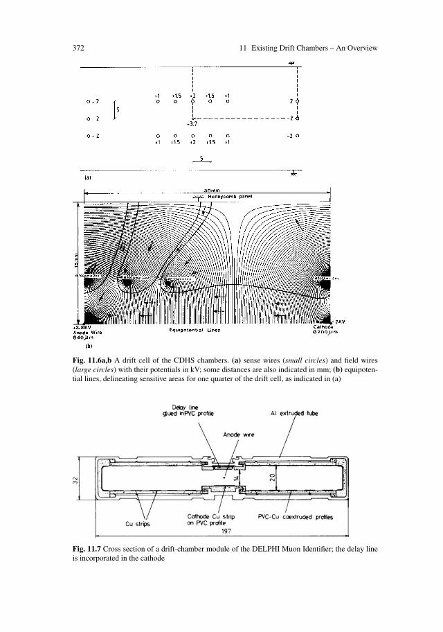
372 11 Existing Drift Chambers – An Overview
Fig. 11.6a,b A drift cell of the CDHS chambers. (a) sense wires (small circles) and field wires(large circles) with their potentials in kV; some distances are also indicated in mm; (b) equipoten-tial lines, delineating sensitive areas for one quarter of the drift cell, as indicated in (a)
Fig. 11.7 Cross section of a drift-chamber module of the DELPHI Muon Identifier; the delay lineis incorporated in the cathode

11.4 Planar Drift Chambers of Type 1 373
Fig. 11.8 A drift cell of the DC1 chambers in the HELIOS experiment; dimensions in mm
double-track separation. The solution adopted involves a slow gas which in turnneeded small drift cells in the high-multiplicity, high-rate environment. We see thedrift cell in Fig. 11.8. It must provide a very homogeneous field because the gas isnot saturated; therefore in each drift cell the eight sense wires are surrounded by alarge number of field wires. In an attempt to reduce the influence of the drift-timevariations, some of the field wires were given such potentials that only a fractionof the ionization along the track was collected on the sense wires. The whole stackconsists of six chambers with three different wire orientations. The performancefigures reveal that the outstanding measuring accuracy of 60 μm per wire, reachedwith the prototype, worsened and became 120 μm in the real experiment where thepresence of many tracks deteriorated the critical field conditions.
The muon chambers of the L3 experiment are the result of a colossal effortto measure the momenta of fast muons with an accuracy of at least δpT/p2
T =4× 10⁻⁴ GeV/c−1, in cylindrical geometry. In the experiment, the radial space be-tween 2.5 and 5.4 m was allocated to this task, inside a magnetic field of 0.5 T. Theprinciple of the solution is sketched in Fig. 11.9; one observes that for the optimalmeasurement of momenta in the magnetic field, the chambers are concentrated atthe inner and outer edges, and in the middle of the radial space (cf. the discussion inSect. 8.2.6). Their local measuring accuracy is increased by sampling each track Ntimes, thus gaining a factor of 1
√N over the accuracy of a single wire – provided,
the relative wire positions are sufficiently well known. For this purpose, the sensewires have been pulled over optically flat edges and are supported in the middle ina controlled fashion. We show in Fig. 11.10 the drift cell of the chamber type in themiddle; it has N = 24 sense wires, 0.9 cm apart and 5.5 m long. Under operatingconditions the Lorentz angle is 19◦.
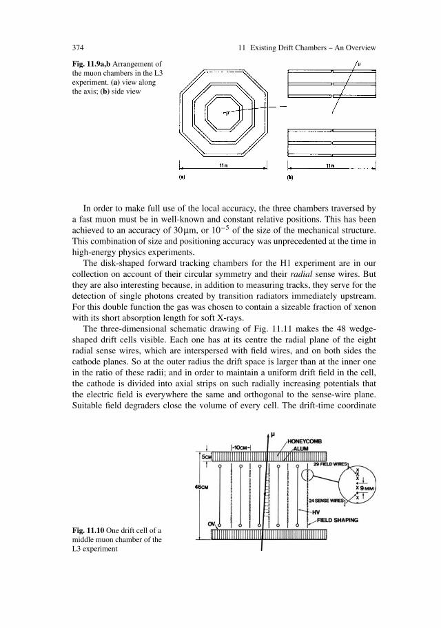
374 11 Existing Drift Chambers – An Overview
Fig. 11.9a,b Arrangement ofthe muon chambers in the L3experiment. (a) view alongthe axis; (b) side view
In order to make full use of the local accuracy, the three chambers traversed bya fast muon must be in well-known and constant relative positions. This has beenachieved to an accuracy of 30μm, or 10−5 of the size of the mechanical structure.This combination of size and positioning accuracy was unprecedented at the time inhigh-energy physics experiments.
The disk-shaped forward tracking chambers for the H1 experiment are in ourcollection on account of their circular symmetry and their radial sense wires. Butthey are also interesting because, in addition to measuring tracks, they serve for thedetection of single photons created by transition radiators immediately upstream.For this double function the gas was chosen to contain a sizeable fraction of xenonwith its short absorption length for soft X-rays.
The three-dimensional schematic drawing of Fig. 11.11 makes the 48 wedge-shaped drift cells visible. Each one has at its centre the radial plane of the eightradial sense wires, which are interspersed with field wires, and on both sides thecathode planes. So at the outer radius the drift space is larger than at the inner onein the ratio of these radii; and in order to maintain a uniform drift field in the cell,the cathode is divided into axial strips on such radially increasing potentials thatthe electric field is everywhere the same and orthogonal to the sense-wire plane.Suitable field degraders close the volume of every cell. The drift-time coordinate
Fig. 11.10 One drift cell of amiddle muon chamber of theL3 experiment
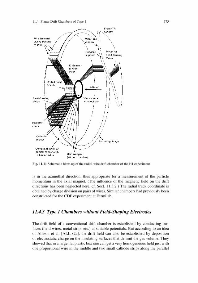
11.4 Planar Drift Chambers of Type 1 375
Fig. 11.11 Schematic blow-up of the radial-wire drift chamber of the H1 experiment
is in the azimuthal direction, thus appropriate for a measurement of the particlemomentum in the axial magnet. (The influence of the magnetic field on the driftdirections has been neglected here, cf. Sect. 11.3.2.) The radial track coordinate isobtained by charge division on pairs of wires. Similar chambers had previously beenconstructed for the CDF experiment at Fermilab.
11.4.3 Type 1 Chambers without Field-Shaping Electrodes
The drift field of a conventional drift chamber is established by conducting sur-faces (field wires, metal strips etc.) at suitable potentials. But according to an ideaof Allison et al. [ALL 82a], the drift field can also be established by depositionof electrostatic charge on the insulating surfaces that delimit the gas volume. Theyshowed that in a large flat plastic box one can get a very homogeneous field just withone proportional wire in the middle and two small cathode strips along the parallel

376 11 Existing Drift Chambers – An Overview
Fig. 11.12 A chamber without field-shaping electrodes
edges (Fig. 11.12). The deposition of charge is straightforward if the insulating sur-faces are backed (on the outside) by grounded plates parallel to the surface. Lookingat Fig. 11.13a, the field lines are as indicated at the moment that HV is applied tothe sense wire. Any positive charge from the wire amplification will travel along thefield lines and will fall onto the insulator and stay there to subsequently change thefield configuration.
This process continues until there are no more field lines pointing at the insu-lator, i.e. the ideal field configuration is reached (Fig. 11.13b). As long as thereis any charge amplification going on at the wire, the ideal field configuration willautomatically be reached. It should be noted that for a thin chamber, the chargeon the wire must finally be equal to the charge on the insulating surface. This im-plies that the gas amplification factor, which is determined by the amount of chargeon the wire, cannot be altered without changing the drift field in the volume. Theproblematic side of this method is in the stability of the field. Although the positivecharges are easily brought into place, they are not so easily removed following smallfluctuations – these may be due to local discharges, bursts of particles, deposits onthe wire, etc., and are probably unavoidable. Allison et al. consider insulators witha non-zero conductivity; these would create a dynamic equilibrium, which wouldbecome a function of the rate of charge deposition.
On the other hand the new principle makes it easy to construct very simple driftchambers. Franz and Grupen [FRA 82] have described the properties of a flat, roundchamber (1.4 cm × 50 cm diam) with only one short (1.4 cm) wire in the centre.
Fig. 11.13a,b Fieldconfiguration (a) during theprocess of charge deposition;(b) ideal field configuration

11.5 Large Cylindrical Drift Chambers of Type 2 377
Becker et al. [BEC 82] have reported measurements with long and thin (20 cm ×1.5 cm) plastic tubes, which could be bent. They have also discussed other applica-tions of the new method. Dorr et al. [DOE 85] analyzed the behaviour of a circularchamber operating in the limited streamer-mode.
11.5 Large Cylindrical Drift Chambers of Type 2
Spanning a large cylindrical volume with wires parallel (or approximately parallel)to the axis requires strong end plates, which hold the wires, carry the combinedpulling force, and keep them in accurate positions. Usually the end plates, togetherwith the outer and inner cylinder mantles, also form the envelope for the gas.The wire feedthroughs that transmit the high voltage and the signals are essentialelements of the construction.
11.5.1 Coordinate Measurement along the Axis – Stereo Chambers
Where charge division and time-difference methods were found insufficient, theidea of varying the wire directions throughout the volume has been widely used.The equivalent of a stack of type 1 chambers with differing wire orientations isa (type 2) ‘axial stereo chamber’. In a cylindrical chamber with many concentriclayers of drift cells, a stereo layer can be formed by rotating the end points onone side of the wire that belong to this layer by the small ‘stereo angle’ α andby keeping the end points fixed on the other side. The cylindrical surface of thiswire layer turns from a cylinder mantle into a hyperbolic surface. The azimuthalwire position becomes a linear function and the radial wire position a quadraticfunction of z to the lowest order of αz counting from the middle of the chamber. Thisinhomogeneity distorts the electric field to some extent. The achievable precisionδ z is equal to the measurement accuracy drϕ achieved in the azimuthal directiondivided by the stereo angle. Hence there is interest in making α as large as theincreasing inhomogeneities permit. In practice, stereo angles are built to plus andminus a few degrees, alternating with zero degrees in successive layers.
Obviously a z measurement can also be provided outside the cylindrical wirechamber with a type 1 chamber. In some experiments special ‘z chambers’ havebeen built for this purpose.
11.5.2 Five Representative Chamberswith (Approximately) Axial Wires
Table 11.2 shows five chambers selected in the spirit described at the beginning ofthis chapter. In quoting performance figures we have indicated (see footnote 1 of thetable) whether they are from early or later stages of the development of the detector.
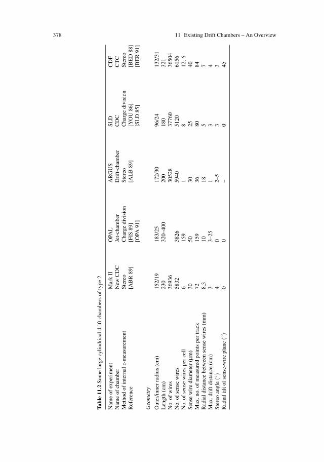
378 11 Existing Drift Chambers – An Overview
Tabl
e11
.2So
me
larg
ecy
lindr
ical
drif
tcha
mbe
rsof
type
2
Nam
eof
expe
rim
ent
Mar
kII
OPA
LA
RG
US
SLD
CD
FN
ame
ofch
ambe
rN
ewC
DC
Jet-
cham
ber
Dri
ft-c
ham
ber
CD
CC
TC
Met
hod
ofin
tern
alz-
mea
sure
men
tSt
ereo
Cha
rge
divi
sion
Ster
eoC
harg
edi
visi
onSt
ereo
Ref
eren
ce[A
BR
89]
[FIS
89]
[AL
B89
][Y
OU
86]
[BE
D88
][O
PA91
][S
LD
85]
[BE
R91
]
Geo
met
ry
Out
er/in
ner
radi
us(c
m)
152/
1918
3/25
172/
3096
/24
132/
31L
engt
h(c
m)
230
320–
400
200
180
321
No.
ofw
ires
3693
630
528
3776
036
504
No.
ofse
nse
wir
es58
3238
2659
4051
2061
56N
o.of
sens
ew
ires
per
cell
615
91
812
;6Se
nse
wir
edi
amet
er(μ
m)
3050
3025
40M
ax.n
o.of
mea
sure
dpo
ints
per
trac
k72
159
3680
84R
adia
ldis
tanc
ebe
twee
nse
nse
wir
es(m
m)
8.3
1018
57
Max
.dri
ftdi
stan
ce(c
m)
33–
251
34
Ster
eoan
gle
(◦)
40
2–5
33
Rad
ialt
iltof
sens
e-w
ire
plan
e(◦
)0
0–
045
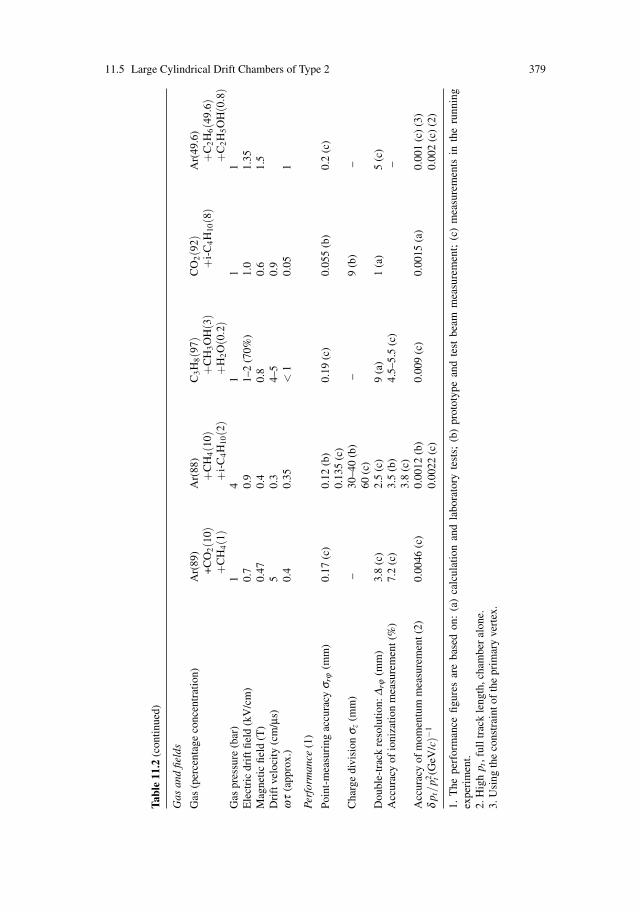
11.5 Large Cylindrical Drift Chambers of Type 2 379
Tabl
e11
.2(c
ontin
ued)
Gas
and
field
s
Gas
(per
cent
age
conc
entr
atio
n)A
r(89
)A
r(88
)C
3H
8(9
7)C
O2(9
2)A
r(49
.6)
+C
O2(1
0)+
CH
4(1
0)+
CH
3O
H(3
)+
i-C
4H
10(8
)+
C2H
6(4
9.6)
+C
H4(1
)+
i-C
4H
10(2
)+
H2O
(0.2
)+
C2H
5O
H(0
.8)
Gas
pres
sure
(bar
)1
41
11
Ele
ctri
cdr
iftfi
eld
(kV
/cm
)0.
70.
91–
2(7
0%)
1.0
1.35
Mag
netic
field
(T)
0.47
0.4
0.8
0.6
1.5
Dri
ftve
loci
ty(c
m/μ
s)5
0.3
4–5
0.9
ωτ
(app
rox.
)0.
40.
35<
10.
051
Perf
orm
ance
(1)
Poin
t-m
easu
ring
accu
racy
σ rϕ
(mm
)0.
17(c
)0.
12(b
)0.
19(c
)0.
055
(b)
0.2
(c)
0.13
5(c
)C
harg
edi
visi
onσ z
(mm
)–
30–4
0(b
)–
9(b
)–
60(c
)D
oubl
e-tr
ack
reso
lutio
n:Δ r
ϕ(m
m)
3.8
(c)
2.5
(c)
9(a
)1
(a)
5(c
)A
ccur
acy
ofio
niza
tion
mea
sure
men
t(%
)7.
2(c
)3.
5(b
)4.
5–5.
5(c
)–
3.8
(c)
Acc
urac
yof
mom
entu
mm
easu
rem
ent(
2)0.
0046
(c)
0.00
12(b
)0.
009
(c)
0.00
15(a
)0.
001
(c)
(3)
δp t
/p2 t
(GeV
/c)−
10.
0022
(c)
0.00
2(c
)(2
)
1.T
hepe
rfor
man
cefig
ures
are
base
don
:(a
)ca
lcul
atio
nan
dla
bora
tory
test
s;(b
)pr
otot
ype
and
test
beam
mea
sure
men
t;(c
)m
easu
rem
ents
inth
eru
nnin
gex
peri
men
t.2.
Hig
hp t
,ful
ltra
ckle
ngth
,cha
mbe
ral
one.
3.U
sing
the
cons
trai
ntof
the
prim
ary
vert
ex.

380 11 Existing Drift Chambers – An Overview
It is not unusual that the prototype performed better than the full chamber eventuallydid in the experiment.
When the momentum-measurement accuracy actually achieved in an experimentis compared to that expected from the point-measuring accuracy, the number ofpoints, and the magnetic field strength (Sect. 8.5.1), it is often not as good as an-ticipated. The overall mechanical accuracy, local and global field distortions, andimperfect calibrations all make their contribution to the momentum-measuring ac-curacy, which sometimes improves only slowly as the apparatus is better and betterunderstood.
11.5.3 Drift Cells
The minimal wire configuration needed to establish the drift and amplification fieldaround the proportional wire (which is at a positive potential) is a group of fieldwires at a negative potential around it. For a drift chamber of type 2, this elementary‘cell’ is repeated to fill the whole volume. Figure 11.14 shows, as an example, driftcells of the ARGUS chamber; the full chamber consists of 5940 cells of this type.Advantages of this arrangement are the high degree of homogeneity over the fullvolume, the fine granularity, which allows the use of single-hit electronics, and thefull track ionization that is employed. On the other hand, the local field around thewire in one cell is not very homogeneous and thus requires a very careful calibrationof the critical relation between drift time and wire–track distance. In Fig. 11.15 wesee the electron drift paths calculated for such a cell type [HAR 84]. They are in theform of spirals, created by the B field parallel to the wires. The contours of equalarrival times are circles near the sense wire, but they are shaped by the field-wiregeometry far from the sense wire. This means in practice that the time–distancerelation for tracks is a function of the orientation of the track with respect to thedrift cell.
The design of the OPAL drift cell goes in the opposite direction (Fig. 11.16).The basic unit is a wedge-shaped sector that fills 15◦ of azimuth over the entireradial space so that the chamber consists of 24 of them. Each sector contains oneradial plane of sense wires which are interspersed by field wires. The sense wiresare actually staggered to resolve the left–right ambiguity. Each sector is limited and
Fig. 11.14 Drift cells of theARGUS chamber. The sensewire is, typically, at 2.9 kVand the cathode wires aregrounded

11.5 Large Cylindrical Drift Chambers of Type 2 381
Fig. 11.15 Drift paths andlines of equal arrival times fora drift cell of the ARGUSchamber. The time lines are15 ns apart
separated from its two neighbours by two common radial planes of cathode wires atsuch radially increasing potentials as to create a homogeneous drift field orthogonalto the central sense/field-wire plane. The inner surface of the enclosing cylindercarries suitable field degraders. This geometry has also been called ‘jet chamber’geometry. In this design the homogeneity is constructed into each sector, which isrelatively large. Close tracks are resolved electronically by using short pulses anddigital pulse-shape analysis. The dilemma of the Lorentz angle is diminished by ahigh gas pressure and a low magnetic field.
The cell design of the new MARK II chamber follows a similar line: radialsense/field-wire planes with radial cathode planes in between, but organized in 132layers, 7.5 cm in radius. This is done in order to be able to create stereo angles inconsecutive layers. There are 972 cells in the chamber. Figure 11.17 shows a cellwith its electron drift trajectories.
Fig. 11.16 A section of the OPAL drift cell with electron drift lines. Upper plane: cathode wires;lower plane: sense/field wires

382 11 Existing Drift Chambers – An Overview
Fig. 11.17 Mark II drift cellwith electron trajectories
The small cell of the SLD drift chamber (Fig. 11.18) is designed to create a betterseparation between the amplification region and the drift region by displacing thefield wires from their position between the sense wires to a position surroundingthem. This is done to create a uniform drift region for the slow gas employed. Herethe good diffusion properties of carbon dioxide have been combined with its lowdrift velocity at high electric fields. Thus the Lorentz angle is kept near 6◦ at thefield of 0.6 T. On the other hand, this imposes severe requirements on the electricfield uniformity, since the drift velocity under these conditions is proportional to theelectric field (‘unsaturated gas’). There are 640 drift cells in the detector. A veryfavourable point-measuring accuracy of 55 μm was obtained with the prototype.This requires that the wire displacements caused by mechanical inaccuracy, gravity,and electrostatic forces as well as by the stereo arrangement are fully controlled tothis precision.
Fig. 11.18 SLD drift cell withelectron drift lines
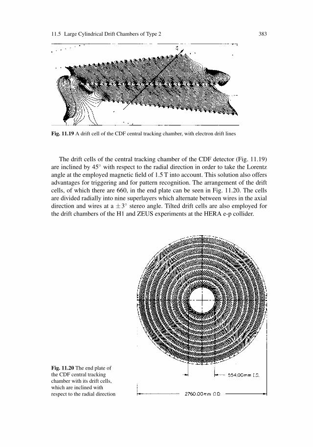
11.5 Large Cylindrical Drift Chambers of Type 2 383
Fig. 11.19 A drift cell of the CDF central tracking chamber, with electron drift lines
The drift cells of the central tracking chamber of the CDF detector (Fig. 11.19)are inclined by 45◦ with respect to the radial direction in order to take the Lorentzangle at the employed magnetic field of 1.5 T into account. This solution also offersadvantages for triggering and for pattern recognition. The arrangement of the driftcells, of which there are 660, in the end plate can be seen in Fig. 11.20. The cellsare divided radially into nine superlayers which alternate between wires in the axialdirection and wires at a ±3◦ stereo angle. Tilted drift cells are also employed forthe drift chambers of the H1 and ZEUS experiments at the HERA e-p collider.
Fig. 11.20 The end plate ofthe CDF central trackingchamber with its drift cells,which are inclined withrespect to the radial direction

384 11 Existing Drift Chambers – An Overview
11.5.4 The UA1 Central Drift Chamber
The detector fills a cylinder, 6 m long and 2.2 m in diameter, which contains thecollider-beam pipe on its axis. Equally horizontal, but at right angles to the beam, isthe magnetic field of 0.7 T (see Fig. 11.21). Along its length, the cylinder is dividedinto three cylindrical sections, each 2 m long: the central section and the two forwardones. The wires are all parallel to the magnetic field and organized in planes accord-ing to the following scheme: the anode planes have alternating sense (35 μm diam)and field (100 μm diam) wires every 5 mm; the cathode planes with 120−μm wires,also every 5 mm, are parallel to the anode planes, leaving drift spaces of 18 cm be-tween them. A peculiarity of the UA1 detector is the orientation of these planes –they are vertical in the central cylinder part and horizontal in the forward parts. Thisarrangement is a consequence of the horizontal magnetic field; the solution opti-mizes the momentum-measuring accuracy, the track curvature being measured bythe drift time. The charge-division technique is used for the coordinate along thewire direction. Filled with a gas mixture of 40% Ar and 60% C4H10 at ambientpressure, the drifting electrons reach a velocity of 5.3 cm/μs under a Lorentz an-gle of 23◦ in their drift field of 1500 V/cm. The total number of wires is 22 800, ofwhich 6110 are sense wires. A stiff vertical track is measured on 100 points and astiff track near the forward directions on up to 180 points.
Fig. 11.21 Geometry of theUA1 central detector

11.5 Large Cylindrical Drift Chambers of Type 2 385
Performance figures were measured in the experiment as follows [NOR 90]: Theaverage point-measuring accuracy in the direction of the drift amounted to 350 μm.The relative accuracy of momentum measurement, which depends very much onthe track orientation, was typically δ p/p = (0.01 GeV/c−1)p for isolated tracks ina favourable direction (obviously, the curvature of tracks that emanate from the in-teraction region under a polar angle of 90◦ and parallel to the magnetic field cannotbe measured.) The electronic two-track resolution limit on a wire was about 5 mm.The coordinate measurement accuracy along the wires was 3.5% r.m.s. of the wirelength after the gain reduction by a factor of three that was necessary when the de-tector had to work in the high-luminosity environment; before this change, 2% hadbeen reached. These numbers illustrate the conflicting requirements of having thesmallest possible space charge in the drift region (small wire amplification) and thebest possible charge-division accuracy (large amplification) at the same time.
Ionization measurements of tracks in this complex detector were limited in accu-racy and were not employed for particle identification.
In Fig. 11.22 we reproduce an event as reconstructed by the computer; the highnumber of measured points along each track make a clear picture even for the com-plicated events created in high-energy hadron collisions – in fact this picture isfamous because it contains the first Z0 particle ever observed. The two arrows markthe electron and the positron into which it decays.
11.5.5 The ATLAS Muon Drift Chambers (MDT)
The ATLAS experiment at the Large Hadron Collider (LHC) will investigatepp-collisions with a total energy of 14 TeV; muons with transverse momenta upto 1 TeV/c will be detected and measured in the muon spectrometer [ATL 97]. Thepurpose of the muon drift chambers is to determine the momenta of the muons asaccurately as possible.
The ATLAS magnet produces a toroidal field in air (field lines going aroundthe beam) which offers a high bending power at much reduced Coulomb scattering
Fig. 11.22 Computer-reconstructed event in the UA1 central detector – the first Z0 particle everobserved is seen to decay into an e+ and an e−. Only one in two wire signals is displayed
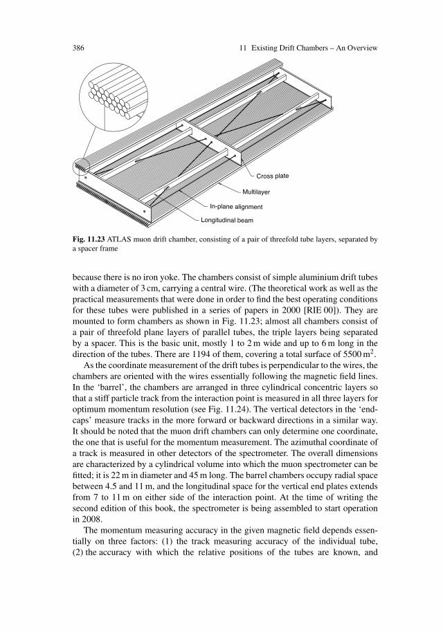
386 11 Existing Drift Chambers – An Overview
Fig. 11.23 ATLAS muon drift chamber, consisting of a pair of threefold tube layers, separated bya spacer frame
because there is no iron yoke. The chambers consist of simple aluminium drift tubeswith a diameter of 3 cm, carrying a central wire. (The theoretical work as well as thepractical measurements that were done in order to find the best operating conditionsfor these tubes were published in a series of papers in 2000 [RIE 00]). They aremounted to form chambers as shown in Fig. 11.23; almost all chambers consist ofa pair of threefold plane layers of parallel tubes, the triple layers being separatedby a spacer. This is the basic unit, mostly 1 to 2 m wide and up to 6 m long in thedirection of the tubes. There are 1194 of them, covering a total surface of 5500 m2.
As the coordinate measurement of the drift tubes is perpendicular to the wires, thechambers are oriented with the wires essentially following the magnetic field lines.In the ‘barrel’, the chambers are arranged in three cylindrical concentric layers sothat a stiff particle track from the interaction point is measured in all three layers foroptimum momentum resolution (see Fig. 11.24). The vertical detectors in the ‘end-caps’ measure tracks in the more forward or backward directions in a similar way.It should be noted that the muon drift chambers can only determine one coordinate,the one that is useful for the momentum measurement. The azimuthal coordinate ofa track is measured in other detectors of the spectrometer. The overall dimensionsare characterized by a cylindrical volume into which the muon spectrometer can befitted; it is 22 m in diameter and 45 m long. The barrel chambers occupy radial spacebetween 4.5 and 11 m, and the longitudinal space for the vertical end plates extendsfrom 7 to 11 m on either side of the interaction point. At the time of writing thesecond edition of this book, the spectrometer is being assembled to start operationin 2008.
The momentum measuring accuracy in the given magnetic field depends essen-tially on three factors: (1) the track measuring accuracy of the individual tube,(2) the accuracy with which the relative positions of the tubes are known, and
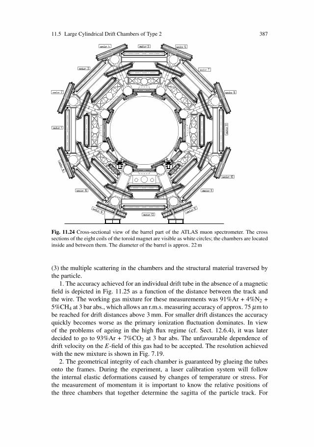
11.5 Large Cylindrical Drift Chambers of Type 2 387
Fig. 11.24 Cross-sectional view of the barrel part of the ATLAS muon spectrometer. The crosssections of the eight coils of the toroid magnet are visible as white circles; the chambers are locatedinside and between them. The diameter of the barrel is approx. 22 m
(3) the multiple scattering in the chambers and the structural material traversed bythe particle.
1. The accuracy achieved for an individual drift tube in the absence of a magneticfield is depicted in Fig. 11.25 as a function of the distance between the track andthe wire. The working gas mixture for these measurements was 91%Ar + 4%N2 +5%CH4 at 3 bar abs., which allows an r.m.s. measuring accuracy of approx. 75 μm tobe reached for drift distances above 3 mm. For smaller drift distances the accuracyquickly becomes worse as the primary ionization fluctuation dominates. In viewof the problems of ageing in the high flux regime (cf. Sect. 12.6.4), it was laterdecided to go to 93%Ar + 7%CO2 at 3 bar abs. The unfavourable dependence ofdrift velocity on the E-field of this gas had to be accepted. The resolution achievedwith the new mixture is shown in Fig. 7.19.
2. The geometrical integrity of each chamber is guaranteed by glueing the tubesonto the frames. During the experiment, a laser calibration system will followthe internal elastic deformations caused by changes of temperature or stress. Forthe measurement of momentum it is important to know the relative positions ofthe three chambers that together determine the sagitta of the particle track. For

388 11 Existing Drift Chambers – An Overview
Fig. 11.25 Measuringaccuracy of an individual drifttube, without a magneticfield. Full circles:measurements; open circles:simulation [RIE 00]
40
50
60
70
80
90
100
110
120
130
0 2 4 6 8 10 12 14
this purpose, the chambers of this ‘tower’ are interconnected by laser rays seenby position-calibrated detectors on the chambers.
3. The mechanical structures for the support of the magnet, the chambers, andall the other detectors of the ATLAS experiment are almost all made of aluminium.They represent a mass of material which causes a lot of Coulomb scattering in ad-dition to that of the chambers proper. It may be quite different from one track toanother; on average it causes relative transverse momentum measurement errorsδ pT /pT typically between 2 and 3%. The aluminium of the chambers themselvescontributes approx. 1%.
The overall momentum-measuring accuracy of the muon spectrometer is calcu-lated to be roughly δ pT /pT = 0.1 at pT = 1 TeV/c, dominated by (1) and (2), and0.03 at pT = 10 GeV/c, dominated by (3).
11.5.6 A Large TPC System for High Track Densities
The NA49 experiment at the CERN SPS accelerator is dedicated to the study ofhadron production on fixed targets in proton-proton, proton-nucleus, and nucleus-nucleus collisions [AFA 99]. A system of 4 large TPCs with a total sensitive volumeof 33 m3 is the main instrument for tracking and dE/dx measurement. The incom-ing beam passes between them, compare Fig. 11.26. Central lead-lead collisions atthe beam momentum of 158 GeV/c per nucleon can produce more than a thousandtracks in one event.
Of the four TPC modules, the two smaller ones are operated inside strong andnot very homogeneous vertical magnetic fields, the two larger ones outside. Thedrift is vertical, the sensitive wire chamber end plates horizontal. The wire grids are

11.5 Large Cylindrical Drift Chambers of Type 2 389
Fig. 11.26 Top view of the four TPCs; the two ‘vertex chambers’ inside the magnetic field are onthe left, the two ‘main chambers’ to both sides of the beam outside the magnetic field are on theright. A central Pb + Pb event is depicted in a slice only 7 mm high around the beam plane, in orderto be able to distinguish tracks in the projection
designed as in the ALEPH TPC but have a reduced distance between pads and sensewires. Their total area amounts to 30 m2. Signals are read out only from the cathodepads of which there are 182 000. A maximum of 234 pad rows is available for themeasurement of fully recorded tracks, but the actual number of signal clusters liesapproximately between 20 and 160, depending on track overlap and kinematics inthe given acceptance region. The authors estimate that an over-all position precisionof about ±0.20 mm has been achieved for isolated tracks, varying with the driftlength between ±0.15 and ±0.28 mm.
The separation of neighbouring tracks is a major challenge in this experiment.The diffusion properties of the gas and the other detector parameters have beendesigned with the aim to reach a charge distribution within typically 5 mm FWHM.The authors show that track pairs with average distances above 1.6 cm are fullydetected, those with distances of 1.0 cm are detected with 50% efficiency. Furtherimprovements seem to be in reach. It is remarkable that the TPC technique can beextended to record tracks in such high particle densities.
This was made possible by an increased density of cathode pads and the associ-ated electronic channels. The entire front-end electronics up to the digital outputs ismounted on the TPC readout chambers, the pad widths being not more than 3.5 or5.5 mm.
The high particle density is a challenging environment also for particle identifi-cation using dE/dx measurements. It is difficult to control the pulse height variationwith drift time which is partly caused by the baseline shift of the electronic signals,partly by the widening of the measured charge clusters at the required threshold,but only to a smaller degree by electron attachment. It is also not easy to correct forelectronic cross-talk at these high particle densities. Despite of these severe condi-tions, the authors are able to report an r.m.s. resolution for the dE/dx measurement
390 11 Existing Drift Chambers – An Overview
of σI = 38%/√
Nc where the number Nc of signal clusters lies between 20 and 160.The method of charge estimation applied is the one of the truncated mean at the50% level. The relativistic plateau is IR = 56% above minimum ionization.
Using the ratio σI/IR as a measure for the ability of particle identification onecan say that the NA49 TPC system reaches a similar level of identification ability asthe detectors listed in Tables 10.3 and 10.4, once the losses of signal clusters fromtrack overlap and acceptance limitation are taken into account.
11.6 Small Cylindrical Drift Chambers of Type 2for Colliders (Vertex Chambers)
Vertex detectors are needed for the measurement of the (primary) interaction vertexor any secondary vertices that may occur in an event from the decay of short-livedparticles. The charm, bottom and τ particles have lifetimes of the order of 10−13 to10−12 s, so the tracks from the secondary vertices will miss the primary vertex bycorrespondingly small distances, which are of the order of 30 to 300 μm. Ideally,vertex chambers should have even better measurement accuracies.
This is the field where the fine-grained solid-state particle detectors with their su-perb spatial resolution are often a better choice than gas drift chambers. These havein their favour the simplicity of a proven technique and a somewhat better resis-tance against high-radiation background. Also they are more easily extended overlarge sensitive areas. Being closer to the interaction point they can often be builtsmaller and with shorter wires than the large axial chambers, so that the wire posi-tion can be extremely well defined. This is a prerequisite for the high measurementaccuracy achieved in the vertex chambers. When measuring the position of a vertexinside the vacuum tube, multiple scattering in the wall of the tube is often a limitingfactor, which depends on the momentum of the extrapolated particle as well as onthe tube radius and the thickness of the wall.
In order to reach the best possible point-measuring accuracy and double-trackresolution, the sense wires have to be as close as possible to each other (cf. thediscussion in Sect. 11.8). The limit imposed by electrostatic stability depends onthe wire length and the detailed electrostatic pattern, and it becomes more severe athigher gas pressures because of the corresponding higher voltages.
To find the correct gas, one has to balance the consequences of a slow ‘cool’gas (see Sects. 2.2.4, 12.1) – slower electronics, high drift field with low diffu-sion, sensitivity to field inhomogeneity through unsaturated drift velocity – withthe consequences of a fast ‘hot’ gas – faster electronics, lower sensitivity to field,temperature and pressure variations.
These questions have been studied in detail for the more recent vertex detec-tors. The chambers listed in Table 11.3 are again intended to represent the differentchoices in the field. They are all axial drift chambers of type 2. The ones that reachthe highest precision are operated with slow cool gas at an elevated pressure. Hayeshas compared vertex drift chambers for the LEP and SLC detectors [HAY 88]. The

11.6 Small Cylindrical Drift Chambers of Type 2 for Colliders 391
Tabl
e11
.3So
me
smal
ldri
ftch
ambe
rsof
type
2(v
erte
xch
ambe
rs)
Nam
eof
expe
rim
ent
UA
2M
AR
KJ
MA
RK
IIO
PAL
MA
CA
LE
PHN
ame
ofch
ambe
rJV
DT
EC
DC
VD
VC
Hst
raw
-VC
ITC
Met
hod
ofz
mea
sure
men
tC
harg
edi
visi
on–
–T
ime
diff
eren
ce–
Tim
edi
ffer
ence
+st
ereo
Ref
eren
ce[B
OS
89]
[AN
D86
][A
LE
89]
[CA
R90
][A
SH87
][D
EL
90]
[AN
D88
a][D
UR
90]
[OPA
91]
[NE
L87
][B
AR
89]
[AN
D88
b]
Geo
met
ry
Out
er/in
ner
radi
us(c
m)
13/4
12/5
17/5
22/1
09/
3.5
28/1
3L
engt
h(c
m)
100
5855
100
4320
0N
o.of
wir
es12
3227
5018
0032
451
36N
o.of
sens
ew
ires
208
168
190
648
324
960
No.
ofse
nse
wir
espe
rce
ll(6
)13
1419
12(6
)1
1Se
nse-
wir
edi
amet
er(μ
m)
2520
2020
3030
No.
ofm
easu
red
poin
tspe
rtr
ack
1314
1918
68
Rad
iald
ista
nce
betw
een
sens
ew
ires
(mm
)(6
)6.
42.
42.
95.
0(5
.3)
6–10
11–1
9M
ax.d
rift
dist
ance
(cm
)2.
51.
3–2.
63
0.8–
1.9
0.35
0.47
–0.6
5St
ereo
angl
e(◦
)0
00
40
0R
adia
ltilt
ofse
nse
wir
epl
ane
(◦)
0±
415
0–
–

392 11 Existing Drift Chambers – An Overview
Tabl
e11
.3(c
ontin
ued)
Gas
and
field
s
Gas
(per
cent
age
conc
entr
atio
ns)
Ar(
60)
CO
2(8
0)C
O2(9
2)A
r(00
)A
r(49
.5)
Ar(
50)
+C
2H
6(4
0)+
i-C
4H
10(2
0)+
C2H
6(8
)+
CH
4(1
0)+
CO
2(4
9.5)
+C
2H
6(5
0)+
i-C
4H
10(2
)+
CH
4(1
)G
aspr
essu
re(b
ar)
11.
92
44
1E
lect
ric
drif
tfiel
d(k
V/c
m)
11.
61.
52.
72–
7(7
0%)
3–5
Mag
netic
field
(T)
00
0.47
0.4
0.6
1.5
Dri
ftve
loci
ty(c
m/μ
s)5.
20.
70.
64.
01–
3(7
0%)
5.0
App
rox.
valu
eof
ωτ
00
0.02
0.1
smal
lsm
all
Perf
orm
ance
(1)
Poin
tmea
suri
ngac
cura
cy15
0(b
)35
(b)
30(b
)50
(b)
70(c
)(4
)10
0(b
)σ r
ϕ(μ
m)
180
(c)
(3)
40(c
)50
(c)
55(c
)45
(c)
(3)
150
(c)
300
(c)
(5)
Cha
rge
divi
sion
ortim
edi
ffer
ence
10(b
)–
–45
(c)
–30
(b)
accu
racy
σ z(m
m)
25(c
)(3
)35
(c)
(5)
Dou
ble-
trac
kre
solu
tion
Δ rϕ
(mm
)2
(b)
0.3
(b)
(7)
0.5
(c)
(8)
2.0
(c)
6.9
11(a
)Im
pact
-par
amet
erac
cura
cy(2
)87
(c)
(3)
130
(c)
σ t(μ
m)
400
(c)
80(b
)30
(c)
30(c
)20
0(c
)(4
)
1.T
hepe
rfor
man
cefig
ures
are
base
don
(a)
calc
ulat
ion
and
labo
rato
ryte
sts;
(b)
prot
otyp
e,co
smic
-ray
orte
st-b
eam
mea
sure
men
ts;
(c)
mea
sure
men
tsin
the
runn
ing
expe
rim
ent.
2.V
erte
xch
ambe
rpl
usm
ain
trac
king
cham
ber
–hi
gh-m
omen
tum
trac
ks.
3.Is
olat
edtr
acks
.4.
Mul
tihad
ron
even
ts,i
nclu
ding
mul
tiple
scat
teri
ng.
5.M
ultih
adro
nev
ents
,ave
rage
mul
tiplic
ity31
to35
.6.
Num
bers
inbr
acke
tsre
fer
toth
eO
PAL
ster
eoce
ll.7.
Tra
ckse
para
tion
atw
hich
50%
ofth
etr
acks
are
corr
ectly
reso
lved
.8.
Tra
ckse
para
tion
atw
hich
appr
ox.1
00%
ofth
etr
acks
are
reso
lved
.
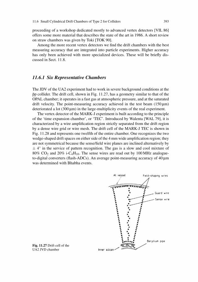
11.6 Small Cylindrical Drift Chambers of Type 2 for Colliders 393
proceeding of a workshop dedicated mostly to advanced vertex detectors [VIL 86]offers some more material that describes the state of the art in 1986. A short reviewon straw chambers was given by Toki [TOK 90].
Among the more recent vertex detectors we find the drift chambers with the bestmeasuring accuracy that are integrated into particle experiments. Higher accuracyhas only been achieved with more specialized devices. These will be briefly dis-cussed in Sect. 11.8.
11.6.1 Six Representative Chambers
The JDV of the UA2 experiment had to work in severe background conditions at thepp collider. The drift cell, shown in Fig. 11.27, has a geometry similar to that of theOPAL chamber; it operates in a fast gas at atmospheric pressure, and at the saturateddrift velocity. The point-measuring accuracy achieved in the test beam (150 μm)deteriorated a lot (300 μm) in the large-multiplicity events of the real experiment.
The vertex detector of the MARK-J experiment is built according to the principleof the ‘time expansion chamber’, or ‘TEC’. Introduced by Walenta [WAL 79], it ischaracterized by a wire amplification region strictly separated from the drift regionby a dense wire grid or wire mesh. The drift cell of the MARK-J TEC is shown inFig. 11.28 and represents one twelfth of the entire chamber. One recognizes the twowedge-shaped drift spaces on either side of the 4 mm wide amplification region; theyare not symmetrical because the sense/field wire planes are inclined alternatively by± 4◦ in the service of pattern recognition. The gas is a slow and cool mixture of80% CO2 and 20% i-C4H10. The sense wires are read out by 100 MHz analogue-to-digital converters (flash-ADCs). An average point-measuring accuracy of 40 μmwas determined with Bhabha events.
Fig. 11.27 Drift cell of theUA2 JVD chamber
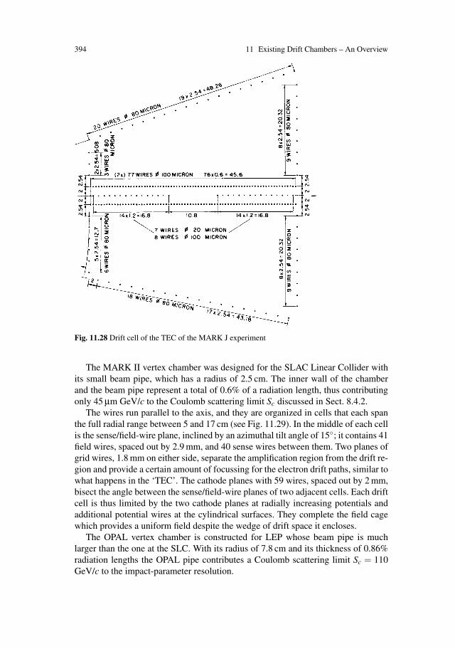
394 11 Existing Drift Chambers – An Overview
Fig. 11.28 Drift cell of the TEC of the MARK J experiment
The MARK II vertex chamber was designed for the SLAC Linear Collider withits small beam pipe, which has a radius of 2.5 cm. The inner wall of the chamberand the beam pipe represent a total of 0.6% of a radiation length, thus contributingonly 45 μm GeV/c to the Coulomb scattering limit Sc discussed in Sect. 8.4.2.
The wires run parallel to the axis, and they are organized in cells that each spanthe full radial range between 5 and 17 cm (see Fig. 11.29). In the middle of each cellis the sense/field-wire plane, inclined by an azimuthal tilt angle of 15◦; it contains 41field wires, spaced out by 2.9 mm, and 40 sense wires between them. Two planes ofgrid wires, 1.8 mm on either side, separate the amplification region from the drift re-gion and provide a certain amount of focussing for the electron drift paths, similar towhat happens in the ‘TEC’. The cathode planes with 59 wires, spaced out by 2 mm,bisect the angle between the sense/field-wire planes of two adjacent cells. Each driftcell is thus limited by the two cathode planes at radially increasing potentials andadditional potential wires at the cylindrical surfaces. They complete the field cagewhich provides a uniform field despite the wedge of drift space it encloses.
The OPAL vertex chamber is constructed for LEP whose beam pipe is muchlarger than the one at the SLC. With its radius of 7.8 cm and its thickness of 0.86%radiation lengths the OPAL pipe contributes a Coulomb scattering limit Sc = 110GeV/c to the impact-parameter resolution.

11.6 Small Cylindrical Drift Chambers of Type 2 for Colliders 395
Fig. 11.29 Drift cell of theVCDV of the MARK IIexperiment
The wire pattern is shown in Fig. 11.30. The chamber is 100 cm long. It has oneaxial and one stereo layer at 20◦. The axial layer between radii of 9.4 and 17.1 cmis of the ‘jet chamber’ type and has 36 radial planes of sense/field wires, each con-taining 12 sense wires spaced out by 5 mm, and the field wires between them. Theleft–right ambiguity, which does not occur when the sense-wire plane is tilted with
Fig. 11.30 Wire pattern of theOPAL vertex chamber
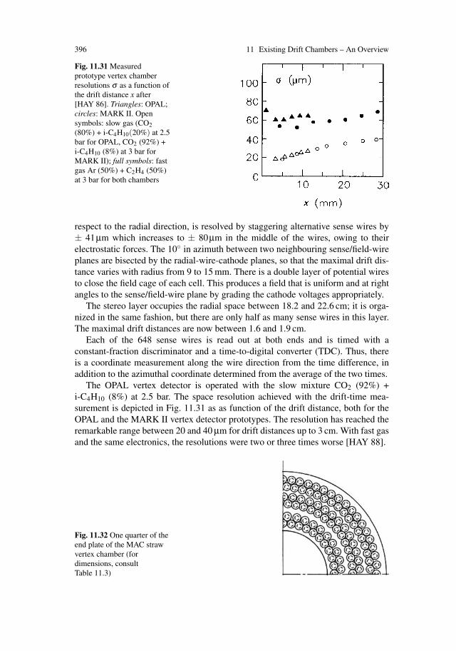
396 11 Existing Drift Chambers – An Overview
Fig. 11.31 Measuredprototype vertex chamberresolutions σ as a function ofthe drift distance x after[HAY 86]. Triangles: OPAL;circles: MARK II. Opensymbols: slow gas (CO2(80%) + i-C4H10(20%) at 2.5bar for OPAL, CO2 (92%) +i-C4H10 (8%) at 3 bar forMARK II); full symbols: fastgas Ar (50%) + C2H4 (50%)at 3 bar for both chambers
respect to the radial direction, is resolved by staggering alternative sense wires by± 41μm which increases to ± 80μm in the middle of the wires, owing to theirelectrostatic forces. The 10◦ in azimuth between two neighbouring sense/field-wireplanes are bisected by the radial-wire-cathode planes, so that the maximal drift dis-tance varies with radius from 9 to 15 mm. There is a double layer of potential wiresto close the field cage of each cell. This produces a field that is uniform and at rightangles to the sense/field-wire plane by grading the cathode voltages appropriately.
The stereo layer occupies the radial space between 18.2 and 22.6 cm; it is orga-nized in the same fashion, but there are only half as many sense wires in this layer.The maximal drift distances are now between 1.6 and 1.9 cm.
Each of the 648 sense wires is read out at both ends and is timed with aconstant-fraction discriminator and a time-to-digital converter (TDC). Thus, thereis a coordinate measurement along the wire direction from the time difference, inaddition to the azimuthal coordinate determined from the average of the two times.
The OPAL vertex detector is operated with the slow mixture CO2 (92%) +i-C4H10 (8%) at 2.5 bar. The space resolution achieved with the drift-time mea-surement is depicted in Fig. 11.31 as as function of the drift distance, both for theOPAL and the MARK II vertex detector prototypes. The resolution has reached theremarkable range between 20 and 40 μm for drift distances up to 3 cm. With fast gasand the same electronics, the resolutions were two or three times worse [HAY 88].
Fig. 11.32 One quarter of theend plate of the MAC strawvertex chamber (fordimensions, consultTable 11.3)

11.7 Drift Chambers of Type 3 397
Fig. 11.33 Drift cells of theALEPH Inner Track Chamber
The drift chambers of the last two examples in our list are again constructedfrom cells that are built around the individual sense wires. The vertex chamber ofthe MAC detector consists of many thin tubes of aluminized Mylar foil with theproportional wire in the centre. These ‘straws’ provide exact cylindrical symmetryand a high degree of electrical shielding between sense wires. Their inner diameteris 6.9 mm, and the wall thickness 50 μm. In Fig. 11.32 we see the layout of thevertex chamber end plate.
The cylindrical geometry produces a drift field that increases with the inversedistance from the wire. The drift velocity therefore also changes, depending on thegas used. In Table 11.3 we have indicated ranges for the field and the velocity thatare valid in the outer 70% of the drift region. In a similar design for the MARK IIIexperiment [ADL 89], the gas mixture was argon–ethane with a more uniform, andhigher, velocity; the achieved point-measuring accuracy was comparable. Toki hasrecently reviewed straw chambers [TOK 90].
The purpose of the ALEPH-ITC is the production of an early trigger signal aswell as precise tracking (a solid-state microstrip detector is mounted in addition).The drift cell is a group of six field wires around each proportional wire, in a flathexagonal arrangement, which is depicted in Fig. 11.33. Each hexagon is character-ized by two shape parameters, the diameters in the radial and in the circumferentialdirections; both vary with the wire layer. A time-difference measurement is the basisfor a determination of the axial coordinate. It takes 0.5 μs for a trigger decision inr−φ and 2.5 μs in r−ϕ − z.
11.7 Drift Chambers of Type 3
An ionization track created in the sensitive gas volume of a type 3 chamber driftsto one of the end faces that delimit the volume. It is there that the amplification andsignal generation take place. Large chambers have drift lengths of one or severalmetres. If a magnetic field is present in a TPC, it is parallel to the drift field, andin this orientation it can greatly improve the transverse diffusion of the travellingelectrons, on account of the magnetic anisotropy of diffusion; see Sect. 2.2.6.
With the length of the drift path we have a correspondingly high drift time – oftenmany tens of microseconds for electrons and several seconds for ions. This makeslong type 3 chambers unsuited for measuring events at very high rates because the
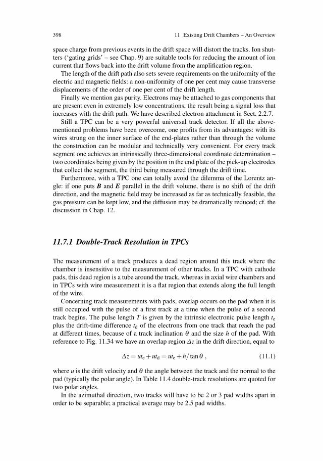
398 11 Existing Drift Chambers – An Overview
space charge from previous events in the drift space will distort the tracks. Ion shut-ters (‘gating grids’ – see Chap. 9) are suitable tools for reducing the amount of ioncurrent that flows back into the drift volume from the amplification region.
The length of the drift path also sets severe requirements on the uniformity of theelectric and magnetic fields: a non-uniformity of one per cent may cause transversedisplacements of the order of one per cent of the drift length.
Finally we mention gas purity. Electrons may be attached to gas components thatare present even in extremely low concentrations, the result being a signal loss thatincreases with the drift path. We have described electron attachment in Sect. 2.2.7.
Still a TPC can be a very powerful universal track detector. If all the above-mentioned problems have been overcome, one profits from its advantages: with itswires strung on the inner surface of the end-plates rather than through the volumethe construction can be modular and technically very convenient. For every tracksegment one achieves an intrinsically three-dimensional coordinate determination –two coordinates being given by the position in the end plate of the pick-up electrodesthat collect the segment, the third being measured through the drift time.
Furthermore, with a TPC one can totally avoid the dilemma of the Lorentz an-gle: if one puts B and E parallel in the drift volume, there is no shift of the driftdirection, and the magnetic field may be increased as far as technically feasible, thegas pressure can be kept low, and the diffusion may be dramatically reduced; cf. thediscussion in Chap. 12.
11.7.1 Double-Track Resolution in TPCs
The measurement of a track produces a dead region around this track where thechamber is insensitive to the measurement of other tracks. In a TPC with cathodepads, this dead region is a tube around the track, whereas in axial wire chambers andin TPCs with wire measurement it is a flat region that extends along the full lengthof the wire.
Concerning track measurements with pads, overlap occurs on the pad when it isstill occupied with the pulse of a first track at a time when the pulse of a secondtrack begins. The pulse length T is given by the intrinsic electronic pulse length teplus the drift-time difference td of the electrons from one track that reach the padat different times, because of a track inclination θ and the size h of the pad. Withreference to Fig. 11.34 we have an overlap region Δz in the drift direction, equal to
Δz = ute +utd = ute +h/ tanθ , (11.1)
where u is the drift velocity and θ the angle between the track and the normal to thepad (typically the polar angle). In Table 11.4 double-track resolutions are quoted fortwo polar angles.
In the azimuthal direction, two tracks will have to be 2 or 3 pad widths apart inorder to be separable; a practical average may be 2.5 pad widths.

11.7 Drift Chambers of Type 3 399
Fig. 11.34 Two inclinedtracks; the first electrons fromtrack 1 arrive on the pad atthe same time as the lastelectrons from track 2
11.7.2 Five Representative TPCs
There are four large cylindrical TPCs that have been built around the interactionpoints of e+e− colliders (PEP-4, TOPAZ, ALEPH, DELPHI); see Table 11.4. Theyare all very similar because their construction followed closely the principles estab-lished by the pioneers in this field, the designers of the PEP-4 TPC. These chambersare cylinders around the colliding beams; the drift direction is parallel to the mag-netic field and to the direction of the incoming particles. The drift volume is dividedin the middle by the high-voltage membrane which is set at a negative potential sothat the circular end plates with their detection electrodes can be kept at earth po-tential (Fig. 11.35). The disposition of the various layers of electrodes in the endplates is seen in Fig. 11.36a, and Fig. 11.36b shows the arrangement of the pads inthe cathode plane in the example of the ALEPH TPC. The inner and outer cylin-der mantles that delimit the gas volume also carry the high-voltage electrode rings,which shape the axial, homogeneous electric drift field.
The four large TPCs differ among each other in two respects: the PEP-4 andTOPAZ TPCs are constructed to work at higher gas pressure and with straight padrows; the ALEPH and DELPHI TPCs have ambient pressure and circular pad rows.The gas pressure is an important choice for any drift chamber (see the discussion inSect. 12.5), but for TPCs one must consider in addition the magnetic anisotropy ofdiffusion – the transverse width of the diffusion cloud increases with the pressure.The circular pad rows in the two TPCs at CERN are an improvement over the (ear-lier) straight rows, since for stiff radial tracks they do not cause the measurementerror that was called the ‘angular pad effect’ in Sect. 7.2.
Whereas the width of the pad determines the number of electronic channels andhence the cost of the project, the length of the pads (extent in the radial direction)is chosen as a balance between the largest possible signal and a loss of accuracyof lower-momentum tracks, owing to the angular pad effect (cf. Sect. 7.3.3). Also,long pads deteriorate the two-track separation for steep tracks (Sect. 11.7.1). Thelong pads in the ALEPH TPC reflect a choice in favour of a larger signal.
The problem of track overlap may be quantified as a loss of tracks rather thanpoints specifying the minimum opening angle Δα measured between two tracks atthe vertex, below which losses are observed. The minimum opening angle is smallerfor pairs with opposite curvature because the magnetic field bends them apart. Such

400 11 Existing Drift Chambers – An Overview
Tabl
e11
.4So
me
TPC
sbu
iltar
ound
colli
ders
Nam
eof
expe
rim
ent
PEP
4T
OPA
ZA
LE
PHD
EL
PHI
CD
F(1)
Ref
eren
ce[L
YN
87]
[KA
M86
][D
EC
90]
[BR
A89
][S
NI
88]
[AV
E89
][S
HI
88]
[AT
W91
][A
AR
90]
[SIE
90]
Geo
met
ry
Out
er/in
ner
radi
us(c
m)
100/
2012
7/30
180/
3111
6/32
21/7
Dri
ftle
ngth
(cm
)2×
100
2×
122
2×
220
2×
134
2×
15N
umbe
rof
sens
ew
ires
2196
2800
6336
1152
384
Sens
e-w
ire
spac
ing
(mm
)4
44
46.
3N
umbe
rof
pads
1382
481
9241
004
2016
038
4Pa
ddi
men
sion
s(r×
rϕ)
(mm
2)
7×
7.5
12×
10(4
)30
×6
8×
741
×14
Max
.no.
ofm
easu
red
poin
tspe
rou
tgoi
ngtr
ack
On
pads
1510
2116
3O
nw
ires
183
175
338
192
24
Gas
and
field
s
Gas
(per
cent
age
frac
tions
)A
r(80
)+
CH
4(2
0)A
r(90
)+
CH
4(1
0)A
r(90
)+
CH
4(1
0)A
r(8
0)+
CH
4(2
0)A
r(50
)+
C2H
6(5
0)G
aspr
essu
re(b
ar)
8.5
3.5
11
1E
lect
ric
drif
tfiel
d(k
V/c
m)
0.55
0.35
0.12
0.15
0.25
Mag
netic
field
(T)
1.32
1.0
1.5
1.2
1.5
Dri
ftve
loci
ty(c
m/μ
s)5
5.3
5.0
6.7
4.3
App
rox.
valu
eof
ωτ
1.5
4.9
75.
43.
5
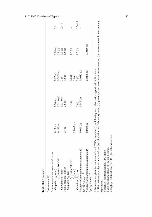
11.7 Drift Chambers of Type 3 401
Tabl
e11
.4(c
ontin
ued)
Perf
orm
ance
(2)
Poin
t-m
easu
rem
ente
rror
radi
altr
acks
On
pads
:σrϕ
(mm
)0.
15(c
)0.
20(c
)0.
17(c
)0.
18(c
)0.
4σ z
(mm
)at
90◦ /
30◦
0.16
/(c)
0.3/
1.0
(c)
0.74
/2(c
)0.
9(c
)–
On
wir
es:σ
z(m
m)
0.3/
1.0(
c)2
(b)
0.9
(c)
0.4–
1D
oubl
e-tr
ack
reso
lutio
n2.
4(c
)2.
5(a
)1.
5(b
)1.
5(c
)–
On
pads
:Δrφ
(cm
)Δ z
(cm
)at
90◦ /
30◦
3/3
(a)
2/6
(b)
1.5
(c)
–Δ α
(mra
d)25
–40
(c)
35(c
)O
nw
ires
:Δz
(cm
)3
(a)
2(b
)1.
5(c
)0.
5–1.
5A
ccur
acy
ofm
omen
tum
mea
sure
men
t(3)
0.00
9(c
)0.
015
(c)
0.00
12(c
)–
δp t
/p2 t
(GeV
/c)−
1
Acc
urac
yof
mom
entu
mm
easu
rem
ent(
5)0.
0065
(c)
0.00
08(c
)0.
0015
(c)
–δ
p t/
p2 t(G
eV/c
)−1
1.N
umbe
rsar
egi
ven
for
each
one
ofth
e8
TPC
s(‘
mod
ules
’),e
ach
havi
ngtw
oha
lves
with
oppo
site
drif
tdir
ectio
ns.
2.T
hepe
rfor
man
cefig
ures
are
base
don
(a)
calc
ulat
ion
and
labo
rato
ryte
sts;
(b)
prot
otyp
ean
dte
st-b
eam
mea
sure
men
ts;
(c)
mea
sure
men
tsin
the
runn
ing
expe
rim
ent
3.H
igh
p t,f
ullt
rack
leng
th,T
PCal
one.
4.Z
ig-z
agsh
ape
alon
grϕ
,dep
th±
2m
m.
5.H
igh
p t,f
ullt
rack
leng
th,T
PCpl
usot
her
dete
ctor
s.
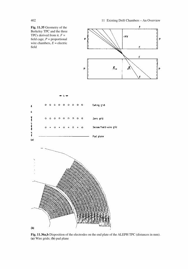
402 11 Existing Drift Chambers – An Overview
Fig. 11.35 Geometry of theBerkeley TPC and the threeTPCs derived from it. F =field cage, P = proportionalwire chambers, E = electricfield
Fig. 11.36a,b Disposition of the electrodes on the end plate of the ALEPH TPC (distances in mm).(a) Wire grids; (b) pad plane
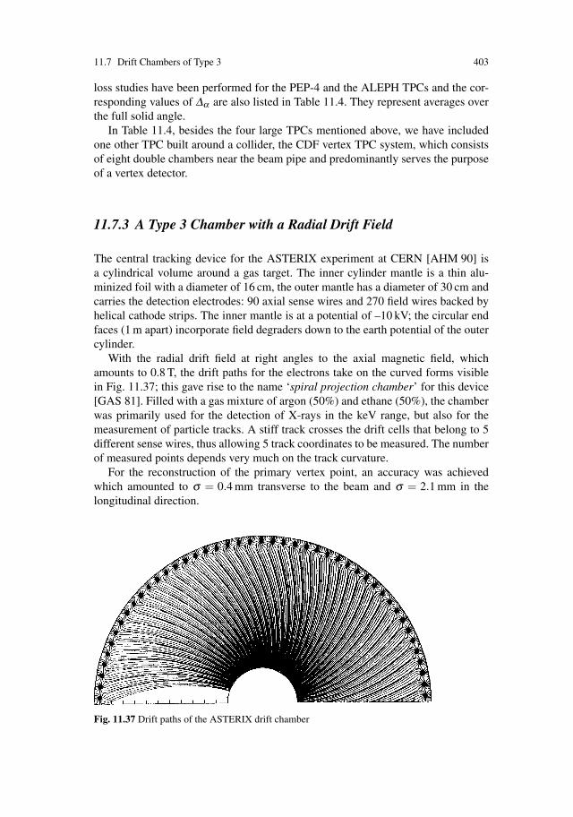
11.7 Drift Chambers of Type 3 403
loss studies have been performed for the PEP-4 and the ALEPH TPCs and the cor-responding values of Δα are also listed in Table 11.4. They represent averages overthe full solid angle.
In Table 11.4, besides the four large TPCs mentioned above, we have includedone other TPC built around a collider, the CDF vertex TPC system, which consistsof eight double chambers near the beam pipe and predominantly serves the purposeof a vertex detector.
11.7.3 A Type 3 Chamber with a Radial Drift Field
The central tracking device for the ASTERIX experiment at CERN [AHM 90] isa cylindrical volume around a gas target. The inner cylinder mantle is a thin alu-minized foil with a diameter of 16 cm, the outer mantle has a diameter of 30 cm andcarries the detection electrodes: 90 axial sense wires and 270 field wires backed byhelical cathode strips. The inner mantle is at a potential of –10 kV; the circular endfaces (1 m apart) incorporate field degraders down to the earth potential of the outercylinder.
With the radial drift field at right angles to the axial magnetic field, whichamounts to 0.8 T, the drift paths for the electrons take on the curved forms visiblein Fig. 11.37; this gave rise to the name ‘spiral projection chamber’ for this device[GAS 81]. Filled with a gas mixture of argon (50%) and ethane (50%), the chamberwas primarily used for the detection of X-rays in the keV range, but also for themeasurement of particle tracks. A stiff track crosses the drift cells that belong to 5different sense wires, thus allowing 5 track coordinates to be measured. The numberof measured points depends very much on the track curvature.
For the reconstruction of the primary vertex point, an accuracy was achievedwhich amounted to σ = 0.4 mm transverse to the beam and σ = 2.1 mm in thelongitudinal direction.
Fig. 11.37 Drift paths of the ASTERIX drift chamber
404 11 Existing Drift Chambers – An Overview
11.7.4 A TPC for Heavy-Ion Experiments
The interaction of a heavy ion of several hundred GeV per nucleon with a fixedtarget often produces hundreds of secondary particles. TPCs have been built to studysuch high-multiplicity events downstream of a fixed target, and we discuss here theBrookhaven chamber as an example [ETK 89]. Like the first TPC, it operates in amagnetic field (0.5 T) parallel to the electric drift field (330 V/cm). However, theelectronic signals are derived not from cathode pads but from short (≈1 cm) anodewires, which are spaced out by 2.54 mm along several parallel straight rows.
There are three thin-walled TPC modules, one behind the other, which areseparate containers of the gas, a mixture of argon (79%), isobutane (16%) anddimethoxymethane (5%) at ambient pressure. In each module the sensitive surfaceis horizontal, and the vertical y coordinate is measured using the drift time. Thex coordinate along each anode row is measured by the wire addresses and a suit-able interpolation, but only the fact of a hit above some discriminator threshold isrecorded. There are twelve anode rows per module, one every 3.8 cm along the zdirection of the incoming beam, and altogether 3072 channels per module.
For the high-multiplicity events a good two-particle separation capability had tobe the essential goal of the construction and of the pattern-recognition programme.The measured result was that two tracks could be separated in 50% of the cases ifthey lay inside the same area that measured 5× 5 mm2 in x–y. The effective r.m.s.point-measuring accuracy amounted to σx = 0.9 mm and σy = 0.75 mm for sec-ondary tracks from Si interaction, whereas isolated beam tracks could be measuredmuch better. The drift velocity was 2.3 cm/μs.
The beam projectiles are fully ionized, and since the gas ionization that theycreate is proportional to the square of their electric charge, there is a beam-ratelimitation in the TPC owing to the build-up of primary positive charge. The authorsobserved that an intensity of 2× 10⁴ oxygen nuclei per AGS spill of 1 s distortedthe tracks to the extent that their apparent sagitta was 0.5 mm in y− z.
In Fig. 11.38 we see the x–y projection of an event with 77 tracks pointing tothe vertex. Whereas it must be very difficult to measure the track reconstructionefficiency, it is impressive to what extent the drift-chamber technique is capable ofreconstructing such complex events.
11.7.5 A Type 3 Chamber as External Particle Identifier
A drift chamber specialized in particle identification, ISIS2, was built by Allisonet al. [ALL 84] as part of the European Hybrid Spectrometer. Located behind afixed target at the SPS machine at CERN, this spectrometer contained two mag-nets and numerous chambers for the measurement of particle tracks and momenta.The purpose of ISIS2 was to precisely record the ionization of the particle tracks,whereas their coordinates would only have to be measured with moderate accuracy.A schematic diagram of this huge and almost empty box is seen in Fig. 11.39. The

11.7 Drift Chambers of Type 3 405
Fig. 11.38 Projection along the beam of a heavy-ion event (silicon beam on gold target) recon-structed in the Brookhaven TPC [ETK 89]
Fig. 11.39 Geometry of the ISIS2 chamber

406 11 Existing Drift Chambers – An Overview
useful volume is 4 m high, 2 m wide and 5.12 m long; it is divided into two driftspaces by a single horizontal wire plane of alternate anodes and cathodes at halfthe chamber height. The particles are supposed to enter the chamber through thefront window, which is part of the field cage that shapes the vertical electric field of500 V/cm. There is no magnetic field. The ionization electrons from each track driftin the uniform field and are amplified on 640 proportional wires connected in pairsto 320 channels of multihit electronics. The chamber is filled with a gas mixture of80% Ar and 20% CO2 at ambient pressure. The performance of this type 3 chamberwas characterized in Chap. 9 in the context of particle identification.
11.7.6 A TPC for Muon-Decay Measurements
In a search for muon–electron conversion, the TRIUMF group employed a TPCwhich was to measure and identify low-momentum electrons and positrons in theregion of 100 MeV/c [BRY 83, HAR 84]. The apparatus surrounded a target foilin which muons were degraded and stopped. The TPC was shaped as a hexagonalcylinder as shown in Fig. 11.40, approximately 70 cm long and equally large in di-ameter, with a central high-voltage plate; the two end plates carried the readout wiresand were at earth potential. The drift field E was 250 V/cm to yield a saturated driftvelocity of 7 cm/μs in an argon–methane gas mixture (80/20). A magnetic field of0.9 T was oriented parallel to E. In order to protect the gas volume as much as pos-sible from positive ions produced at the anode wires, a double layer of a monopolargating grid (see Sect. 9.2.1) was mounted at the entrance of the amplification region.It was kept ‘closed’ until a trigger signal arrived.
Fig. 11.40 A perspective viewof the TRIUMF TPC[BRY 83]. (1) Magnet iron;(2) coil; (3) outer triggerscintillators; (4) outer triggerproportional counters; (5)end-cap support frame; (6, 8)field cage wires; (7) centralhigh-voltage plane; (9) innertrigger scintillators; (10) innertrigger proportional wirechamber; (11) TPC end-capproportional wire modules

11.8 Chambers with Extreme Accuracy 407
11.8 Chambers with Extreme Accuracy
The accuracy of coordinate measurement is the crucial point of most drift cham-bers. As we have discussed throughout this book, the essential parameters are thoseitemized in Table 11.5. The choices open to the designer that correspond to theseparameters are quoted in the right-hand column of the table. We notice that some ofthem represent conflicting requirements. For example, slow gas is not saturated atpractical electric fields, and reduced sense-wire distances cause larger wire bowingowing to electrostatic forces that add to the gravitational sag. There are of courseall the other important boundary conditions of the particle experiment – interac-tion rate, space available, radiation material tolerable, and, last but not least, cost –which further restrict the choices to be made in the quest for the very best accuracy.Therefore, it is a much harder goal to achieve good accuracy in a drift chamber thatis part of a particle experiment than in a test chamber built for a more specializedinvestigation. The problems connected with small wire distances and mechanicalaccuracy are obviously better solved in chambers with small dimensions. For thesereasons, the chambers that have reached extreme values of accuracy are small andspecialized.
A chamber containing xenon gas under a pressure of 20 atm was presented byBaskakov et al. and is depicted in Fig. 11.41 [BAS 79]. It is the most precise driftchamber known to us. Its two anode wires have no electrical amplifiers attached tothem but are viewed by two photomultipliers, which register the light pulse emitted
Table 11.5 Factors relevant for accuracy and corresponding choices of design parameters
Diffusion: Gas with low diffusionSmall drift lengthElevated gas pressureMagnetic field
Drift-path variations: Reduced sense-wire distanceFocussing of drift trajectoriesDrift-path restrictions
Ionization clustering: Elevated gas pressureTime measurement: Fast electronics
Slow gasOptimal estimator
Avalanche localization: Increased number of channelsNarrow avalancheAccurate pulse-height measurementOptimal estimator
Uniformity of drift velocity: Homogeneous electric fieldNo free charges in drift volumeSmall field-wire distancesMechanical accuracySaturated drift velocity
Knowledge of wire positions: Mechanical accuracyShort wiresControlled wire sag

408 11 Existing Drift Chambers – An Overview
Fig. 11.41 Cross section of a drift chamber based on electroluminescence by Baskakov et al.[BAS 79], which had two sense wires
by the avalanche. Drift chambers based on electroluminescence had previously beenstudied by Charpak, Majewski and Sauli [CHA 75]; these are suitable for high par-ticle rates because the emission of light in the high electric field of the anode wire isso strong (especially at high gas pressure) that only little or no charge amplificationis necessary. However, large systems of such drift chambers have not yet been built.
With their chamber, Baskakov et al. were able to achieve an average accuracy of18 μm on one wire over a sensitive drift length between 10 and 35 mm (16 μm at20 mm). This accuracy comes mainly from the low drift velocity of 0.13 cm/μs andthe small diffusion at this pressure. The sensitive area was nearly 4×4 cm2.
Fig. 11.42a,b Precision drift chamber by Belau et al. [BEL 82]. (a) Wire configuration of threecells; (b) spatial resolution of a single wire as a function of gas pressure

References 409
A more conventional model is the precision chamber built by Belau et al. forthe recording of particles behind a target [BEL 82]. It operates with a gas mixtureof 75% propane and 25% ethylene at 4 atm pressure and presents a sensitive areaof 10 × 10cm2. The proportional wires (spaced 1.3 mm) are arranged in 6 hori-zontal planes, the cathode wires in parallel planes, creating 12 drift spaces 8 mmhigh and 50 mm deep, and one central insensitive space for a high-intensity beam(Fig. 11.42a). The achieved accuracy was 23 μm per wire after eliminating or cali-brating the inhomogeneous drift regions near the wires (18% of the volume). Thisaccuracy was obtained with a fast gas (drift velocity 5 cm/μs) and correspondinglyfast electronics (rise time 0.8 ns) on 60 channels. The mechanical accuracy is basedon ceramic spacers for the wires, ground to a precision of a few microns. The vari-ation of the achieved measuring accuracy with gas pressure is seen in Fig. 11.42b.
References
[ABR 89] G. Abrams, The MARK II detector for the SLC, Nucl. Instrum. Methods Phys. Res.A 287, 55 (1989)
[ADE 90] B. Adeva et al., The construction of the L3 experiment, Nucl. Instrum. Methods Phys.Res. A 289, 35 (1990)
[ADL 89] J. Adler et al., The MARK III vertex chamber, Nucl. Instrum. Methods Phys. Res. A276, 42 (1989)
[AFA 99] S. Afanasiev et al. (NA49 Collaboration), The NA49 large acceptance hadron detec-tor, Nucl. Instr. and Meth. Phys. Res. A 430, 210-244 (1999)
[AHM 90] S. Ahmad et al., The ASTERIX spectrometer at LEAR, Nucl. Instrum. Methods Phys.Res. A 286, 76 (1990)
[ALB 89] H. Albrecht et al., ARGUS – a universal detector at DORIS II, Nucl. Instrum.Methods Phys. Res. A 275, 1 (1989)
[ALE 89] J. P. Alexander et al., The Mark II vertex drift chamber, Nucl. Instrum. Methods Phys.Res. A 283, 519 (1989)
[ALL 74] W.W.M. Allison, C.B. Brooks, J.N. Bunch, J.H. Cobb, J.L. Lloyd, R.W. Fleming, Theidentification of secondary particles by ionisation sampling, Nucl. Instrum. Methods119, 499 (1974)
[ALL 82] W.W.M. Allison, Relativistic particle identification by dE/dx: the fruits of experiencewith ISIS, in Int. Conf. for Colliding Beam Physics, SLAC, 61 (1982)
[ALL 82a] J. Allison, R.J. Barlow, C.K. Bowdery, I. Duerdoth, P.G. Rowe, An electrodeless driftchamber, Nucl. Instrum. Methods 201, 341 (1982)
[ALL 84] W.W.M. Allison, C.R. Brooks, P.D. Shield, M. Aguilar-Benitez, C. Willmott,J. Dumarchez, M. Schouten, Relativistic charged particle identification with ISIS2,Nucl. Instrum. Methods Phys. Res. 224, 396 (1984)
[AND 86] H. Anderhub et al., A time expansion chamber as a vertex detector for the experimentMARK J at DESY, Nucl. Instrum. Methods Phys. Res. A 252, 357 (1986)
[AND 88a] H. Anderhub et al., A time expansion chamber as a vertex detector, Nucl. Instrum.Methods Phys. Res. A 263, 1 (1988)
[AND 88b] H. Anderhub et al., Operating experience with the MARK-J time expansion chamber,Nucl. Instrum. Methods Phys. Res. A 215, 50 (1988)
[ASH 87] W.W. Ash et al., Design, construction, prototype tests and performance of a vertexchamber for the MAC detector, Nucl. Instrum. Methods Phys. Res. A 261, 399 (1987)
[ATL 97] ATLAS muon spectrometer: Technical Design Report, CERN, Geneva, Switzerland,CERN/LHC 97–22, 1997
410 11 Existing Drift Chambers – An Overview
[ATW 91] W.B. Atwood et al., Performance of the ALEPH Time Projection Chamber, Nucl.Instrum. Methods Phys. Res. A 306, 446 (1991)
[AVE 89] R.E. Avery, Bose–Einstein Correlations of pions in e+e− annihilation at 29 GeVcenter-of-mass energy, PhD thesis, University of California, 1989, also LBL preprint26593
[BAR 89] G.J. Barber et al., Performance of the three-dimensional readout of the ALEPH innertracking chamber, Nucl. Instrum. Methods Phys. Res. A 279, 212 (1989)
[BAS 79] V. I. Baskakov et al., The electroluminescenting drift chamber with spatial resolution16 μm, Nucl. Instrum. Methods 158, 129 (1979)
[BEC 82] Ch. Becker, W. Weihs, G. Zech, Wireless drift tubes, electrodeless drift chambers andapplications, Nucl. Instrum. Methods 200, 335 (1982)
[BEC 89] G.A. Beck et al., Radial wire drift chambers for the H1 forward track detector atHERA: Design, construction and performance, Nucl. Instrum. Methods Phys. Res. A283, 471 (1989)
[BED 88] F. Bedeschi et al., Design and construction of the CDF central tracking chamber,Nucl. Instrum. Methods Phys. Res. A 268, 50 (1988)
[BEL 82] E.R. Belau, W. Blum, Z. Hajduk, T.W.L. Sanford, Construction and performance of asmall drift chamber with 23 μm spatial resolution, Nucl. Instrum. Methods 192, 217(1982)
[BER 91] J.P. Berge, Private communication, Sept. 1991[BET 86] D. Bettoni et al., Drift chambers with controlled charge collection geometry for the
NA34/HELIOS experiment, Nucl. Instrum Methods Phys. Res. A 252, 272 (1986)[BOS 89] F. Bosi et al., Performance of the UA2 Jet Vertex Detector at the CERN Collider,
Nucl. Instrum. Methods Phys. Res. A 283, 532 (1989)[BRA 89] C. Brand et al., The DELPHI time projection chamber, Nucl. Instrum. Methods Phys.
Res. A 283, 567 (1989)[BRE 69] T. Bressani, G. Charpak, D. Rahm and C. Zupancic;, Track localization by means of a
drift chamber, in Proc. of the International Seminar on ‘Filmless Spark and StreamerChambers’ (April 1969) (Joint Institut for Nuclear Research, Dubna, USSR, 1969)p. 275
[BRE 75] A. Breskin, G. Charpak, F. Sauli, M. Atkinson, G. Schultz, Recent observations andmeasurements with high-accuracy drift chambers, Nucl. Instrum. Methods 124, 189(1975)
[BRE 78] A. Breskin, G. Charpak, F. Sauli, A solution to the right–left ambiguity in drift cham-bers, Nucl. Instrum. Methods 151, 473 (1978)
[BRY 83] D. Bryman et al., The time projection chamber at TRIUMF, in Proceedings ofa Workshop on ‘The Time Projection Chamber’, ed. by J.A. Macdonald held atTRIUMF, Vancouver, Canada, June 1983. AIP Conference Proceedings No. 108(American Institute of Physics, New York 1984)
[CAR 90] J.R. Carter et al., The OPAL vertex drift chamber, Nucl. Instrum. Methods Part. Phys.A 286, 99 (1990) and private communication from J. Carter
[CHA 68] G. Charpak, R. Bouclier, T. Bressani, J. Favier. C. Zupancic, The use of multiwireproportional counters to select and localize charged particles, Nucl. Instrum. Methods62, 262 (1968)
[CHA 70] G. Charpak, D. Rahm and H. Steiner, Some developments in the operation of mul-tiwire proportional chambers, Nucl. Instrum. Methods 80, 13 (1970) (received 13November 1969)
[CHA 73] G. Charpak, F. Sauli, W. Duinker, High accuracy drift chambers and their use instrong magnetic fields, Nucl. Instrum. Methods 108, 413 (1973)
[CHA 75] G. Charpak, S. Majewski and F. Sauli, The scintillating drift chamber: A new tool forhigh-accuracy, very-high-rate particle localization, Nucl. Instrum. Methods 126, 381(1975)
[CHA 84] G. Charpak and F. Sauli, High-resolution electronic particle detectors, Annu. Rev.Nucl. Part. Sci. 34, 285 (1984)

References 411
[CLA 76] A.R. Clark et al. (Johns Hopkins University, Lawrence Berkeley Laboratory,University of California at Los Angeles, University of California at Riverside, YaleUniversity), Proposal for a PEP facility based on the time projection chamber,SLAC-PUB-5012 (1976)
[DAU 86] E. Daubie et al., Drift chambers with delay line readout, Nucl. Instrum. MethodsPhys. Res. A 252, 435 (1986)
[DAV 79] W. Davies-White, G.E. Fischer, M.J. Lateur, R.H. Schindler, R.F. Schwitters,J.L. Siegrist, H. Taureg, H. Zaccone, D.L. Hartill, A large cylindrical drift chamberfor the MARK II detector at SPEAR, Nucl. Instrum. Methods 160, 227 (1979)
[DEC 90] D. Decamp et al., ALEPH, A detector for electron–positron annihilation at LEP, Nucl.Instrum. Methods Phys. Res. A 294, 121 (1990)
[DEL 91] DELPHI Collaboration, The DELPHI detector at LEP. Nucl. Instrum. Methods Phys.Res. A 303, 233 (1991)
[DOE 85] R. Dorr, C. Grupen, A. Noll, Characteristics of a multiwire circular electrodeless driftchamber, Nucl. Instrum. Methods Phys. Res. A 238, 238 (1985)
[DUR 90] D. Durret et al., Calibration and performance of the MARK-II drift chamber vertexdetector, SLAC-PUB 5259, LBL 29108 (1990)
[ETK 89] A. Etkin et al., Modular TPC’s for relativistic heavy-ion experiments, Nucl. Instrum.Methods Phys. Res. A 283, 557 (1989)
[FAB 90] C. Fabjan, private communication, April 1990[FIS 89] H.M. Fischer et al., The OPAL jet chamber, Nucl. Instrum. Methods Phys. Res. A
283, 492 (1989)[FLU 81] G. Flugge, B. Koppitz, R. Kotthaus, H. Lierl. Review of contributed papers for ex-
perimentation at LEP, Phys. Scr. 23, 499 (1981)[FRA 82] A. Franz and C. Grupen, Characteristics of a circular electrodeless drift chamber,
Nucl. Instrum. Methods 200, 331 (1982)[GAS 81] U. Gastaldi, The spiral projection chamber (SPC): A central detector with high reso-
lution and granularity suitable for experiments at LFP, Nucl. Instrum. Methods 188,459 (1981)
[GRA 89] H. Grasser et al., Simultaneous track reconstruction and electron identification in theH1 radial drift chambers, Nucl. Instrum. Methods Phys. Res. A 283, 622 (1989)
[HAR 84] G. Harder, Optimierung der Ortsauflosung der zylindrischen Driftkammer des De-tektors ARGUS, Diploma Thesis, DESY Internal Report F15-84/01 (unpublished)
[HAY 88] K.G. Hayes, Drift chamber vertex detectors for SLC/LEP, Nucl. Instrum. MethodsPhys. Res. A 265, 60 (1988)
[KAM 86] T. Kamae et al., The TOPAZ time projection chamber, Nucl. Instrum. Methods Phys.Res. A 252, 423 (1986)
[LYN 87] G. Lynch, Performance of the PEP-4 TPC, Talk given in MPI Munich, 22 June 1987[MAR 77] G. Marel et al., Large planar drift chambers, Nucl. Instrum. Methods 141, 43 (1977)[MUL 73] J. Mulvey, Comments on particle identification using the relativistic rise of ioniza-
tion energy loss, in Int. Conf. on Instrumentation for High Energy Physics, ed. byStipcich and Stanislao, held in Frascati, Italy (Lab. Naz. del Com. Naz. per I’EnergiaNucleare, Frascati 1973), p. 259
[NEL 87] H.N. Nelson, Design and construction of a vertex chamber, and measurement of theaverage B hadron life time, SLAC 322 (1987) (unpublished)
[NOR 90] A. Norton, private communication, July 1990[NYG 74] D.R. Nygren, Proposal to investigate the feasibility of a novel concept in particle
detection, LBL internal report, Berkeley, February 1974[NYG 83] D.R. Nygren, TPC workshop summary, in Proceedings of a Workshop on ‘The Time
Projection Chamber’, ed. by J.A. Macdonald held at TRIUMF, Vancouver, Canada,June 1983. AIP Conference Proceedings No. 108 (American Institute of Physics,New York 1984)
[OPA 91] OPAL Collaboration, The OPAL detector at LEP, Nucl. Instrum. Methods Phys. Res.A 305, 275 (1991)

412 11 Existing Drift Chambers – An Overview
[RIE 00] W. Riegler et al., Resolution limits of drift tubes, Nucl. Instr. and Meth. in Phys.Res. A 443, 156-163 (2000), W. Riegler et al., Front-end electronics for drift tubes inhigh-rate environment, Nucl. Instr. and Meth. in Phys. Res. A 446, 555-559 (2000),M. Aleksa et al., Rate effects in high-resolution drift chambers, Nucl. Instr. and Meth.in Phys. Res. A 446, 435-443 (2000), M. Deile et al., Dependence of drift tube per-formance on the anode wire diameter, Nucl. Instr. and Meth. in Phys. Res. A 449,528-535 (2000)
[SHI 88] A. Shirahashi et al., Performance of the TOPAZ time projection chamber, IEEETrans. NS-35, 414 (1988)
[SIE 90] P. Siegrist, CERN, private communication, September 1990[SLD 85] SLD Design Report, SLAC Report 273 (revised 1985)[SNI 88] F. Snider et al., The CDF Time Projection Chamber system, Nucl. Instrum. Methods
Phys. Res. A 268, 75 (1988)[TOK 90] W.H. Toki, Review of straw chambers, in Proceedings of the 5th Int. Conf. for Col-
liding Beam Physics, Novosibirsk (USSR), March 1990; also as: SLAC preprintSLAC-PUB-5232 (1990)
[VIL 86] F. Villa (ed.), Vertex Detectors, Proceedings of a Workshop for the INFN EloisatronProject, held September 1986 (Plenum, New York London 1988)
[WAG 81] A. Wagner, Central detectors, Phys. Ser. 23, 446 (1981)[WAL 71] A.H. Walenta, J. Heintze and B. Schurlein, The multiwire drift chamber, a new type
of multiwire proportional chamber, Nucl. Instrum. Methods 92, 373 (1971) (received27 November 1970)
[WAL 78] A.H. Walenta, Left–right assignment in drift chambers and MWPC’s using inducedsignals. Nucl. Instrum. Methods 151, 461 (1978)
[WAL 79] A.H. Walenta, The time expansion chamber and single ionization cluster measure-ment, IEEE Trans. Nucl. Sc. NS 26, 73 (1979)
[WIL 86] H.H. Williams, Design principles of detectors at colliding beams, Annu. Rev. Nucl.Part. Sc. 36, 361 (1986)
[YOU 86] C.C. Young et al., Performance of the SLD central driftchamber prototype, IEEETransactions Nucl. Sc. 33, 176 (1986)
Chapter 12Drift-Chamber Gases
Gas is the medium in which the processes of ionization, drift and amplificationdevelop. We have discussed these processes in previous parts of this book. Here wewant to present some additional practical information relevant to the choice of gasmixtures and their pressure, and relevant to the impurities that can be tolerated inthe gas.
12.1 General Considerations Concerning the Choiceof Drift-Chamber Gases
There are many gas mixtures that are successfully used in drift chambers. The tablesin Chap. 11 contain a representative collection. Often we find the noble gas argonmixed with some quenching organic molecular gas. But purely organic mixturesare also in use. These gases fulfil the basic requirement that the electron lifetime issufficiently long and that a stable amplification process exists.
An important choice has to be made with regard to the drift velocity and its de-pendence on the electric field. A highly preferable situation arises if the drift velocityvaries little with the field, for then the coordinate measurement is less dependent onthe unavoidable field gradients, and on the pressure and temperature variations ofthe gas. This happens at the maximum of the velocity–field relation (‘saturated driftvelocity’). Figure 12.1 shows the drift velocity of argon–isobutane mixtures, whichhave this desirable property over a relatively long range of E field.
At these high velocities – typically 5 cm/μs – a fast time measurement is a ne-cessity. If one wants to relax this requirement, one can reduce the drift field, and thedrift velocity is no longer saturated, with the consequence that it depends on spacecharge and other changes of the drift field, thus requiring very careful calibrations.
The ‘dilemma of the Lorentz angle’ comes into sight here (see Sect. 11.3.2). Ifthe electric and magnetic fields are orthogonal one may wish to achieve a small driftvelocity at a high E field in order to keep the Lorentz angle small, cf. (2.7), (2.11).
W. Blum et al., Particle Detection with Drift Chambers, 413doi: 10.1007/978-3-540-76684-1 12, c© Springer-Verlag Berlin Heidelberg 2008

414 12 Drift-Chamber Gases
Fig. 12.1. Drift velocity as a function of the drift field, for various argon–isobutane mixtures[BRE 74]
A high E field at small electron energy must be the goal in the interest of alow diffusion width; cf. the discussion following (2.63). The last two requirementscombine well in the ‘cold’ gas mixtures based on carbon dioxide or dimethylether.In these, the random electron velocities and the drift velocity are much lower thanin the ‘hot’ gases at the same field strength. The cold gases have the disadvantagethat an operating point must be found in the unsaturated situation. High E fields aremore difficult to handle, since spurious discharges are a threat to the reliability of achamber. High E fields also cause electrostatic wire displacements; these are largerfor greater wire lengths.
In order to give an overview of achievable diffusion limits we reproduce inFig. 12.2 the characteristic electron energies calculated by Paladino and Sadoulet[PAL 75] for the pure gases Ar, CH4 and CO2, and for various argon–isobutane mix-tures. The width of the diffusion after 1 cm of drift, calculated according to (2.63),is shown in Fig. 12.3.
In TPCs, where the E and B fields are parallel, there is an advantage in having ahigh value of ωτ , or a high product of the B field and the mobility (cf. Sect. 2.1).One reason is the enormous suppression factor for the transverse diffusion constant(2.72), another has to do with the track distortions caused by imperfections in theuniformity of the magnetic field. Since in a good solenoid the inhomogeneities arepredominantly radial (not azimuthal), the distortions of the curvature of radial tracksare suppressed by one power of ωτ; see (2.6).
Argon–methane mixtures with small CH4 concentrations can be used in the sat-urated situation of the drift velocity, and there they exhibit large values of τ . It canbe seen in Table 11.4 that such gas mixtures have actually been chosen for all thelarge TPCs.
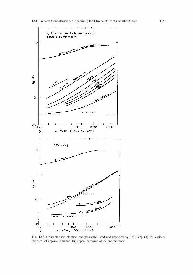
12.1 General Considerations Concerning the Choice of Drift-Chamber Gases 415
Fig. 12.2. Characteristic electron energies calculated and reported by [PAL 75]. (a) for variousmixtures of argon–isobutane; (b) argon, carbon dioxide and methane
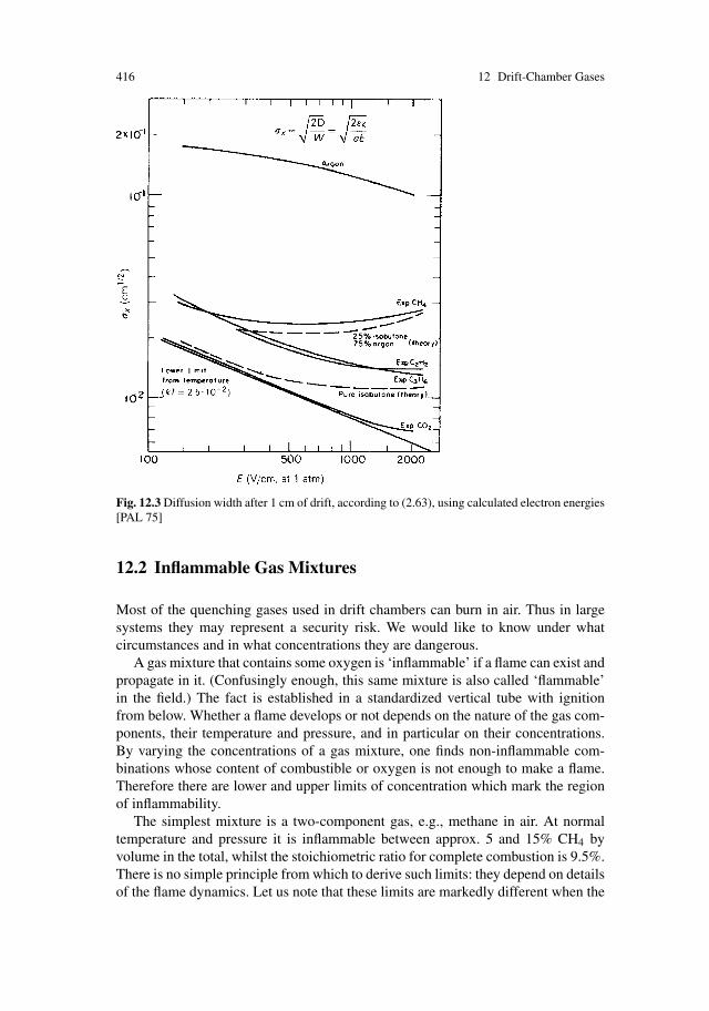
416 12 Drift-Chamber Gases
Fig. 12.3 Diffusion width after 1 cm of drift, according to (2.63), using calculated electron energies[PAL 75]
12.2 Inflammable Gas Mixtures
Most of the quenching gases used in drift chambers can burn in air. Thus in largesystems they may represent a security risk. We would like to know under whatcircumstances and in what concentrations they are dangerous.
A gas mixture that contains some oxygen is ‘inflammable’ if a flame can exist andpropagate in it. (Confusingly enough, this same mixture is also called ‘flammable’in the field.) The fact is established in a standardized vertical tube with ignitionfrom below. Whether a flame develops or not depends on the nature of the gas com-ponents, their temperature and pressure, and in particular on their concentrations.By varying the concentrations of a gas mixture, one finds non-inflammable com-binations whose content of combustible or oxygen is not enough to make a flame.Therefore there are lower and upper limits of concentration which mark the regionof inflammability.
The simplest mixture is a two-component gas, e.g., methane in air. At normaltemperature and pressure it is inflammable between approx. 5 and 15% CH4 byvolume in the total, whilst the stoichiometric ratio for complete combustion is 9.5%.There is no simple principle from which to derive such limits: they depend on detailsof the flame dynamics. Let us note that these limits are markedly different when the
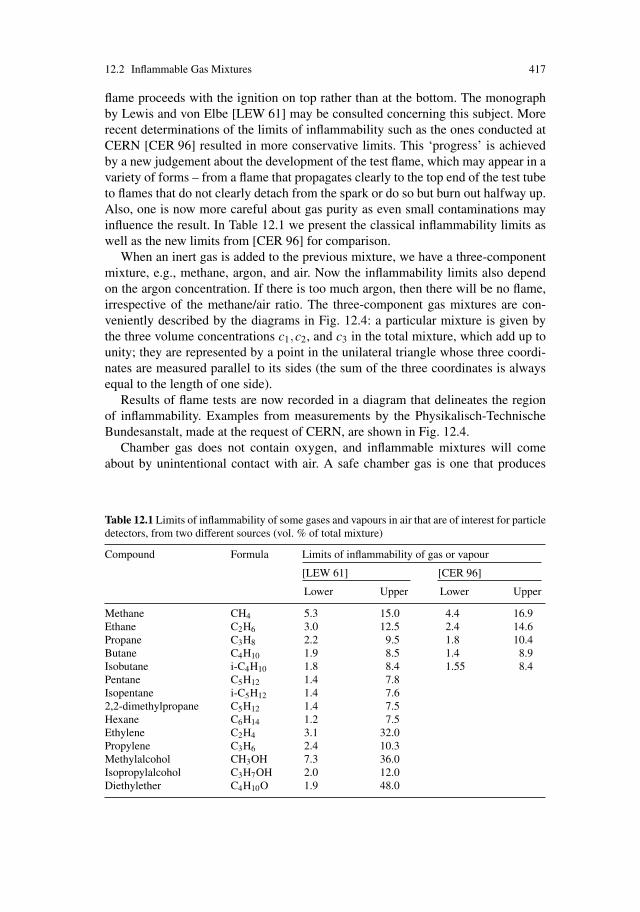
12.2 Inflammable Gas Mixtures 417
flame proceeds with the ignition on top rather than at the bottom. The monographby Lewis and von Elbe [LEW 61] may be consulted concerning this subject. Morerecent determinations of the limits of inflammability such as the ones conducted atCERN [CER 96] resulted in more conservative limits. This ‘progress’ is achievedby a new judgement about the development of the test flame, which may appear in avariety of forms – from a flame that propagates clearly to the top end of the test tubeto flames that do not clearly detach from the spark or do so but burn out halfway up.Also, one is now more careful about gas purity as even small contaminations mayinfluence the result. In Table 12.1 we present the classical inflammability limits aswell as the new limits from [CER 96] for comparison.
When an inert gas is added to the previous mixture, we have a three-componentmixture, e.g., methane, argon, and air. Now the inflammability limits also dependon the argon concentration. If there is too much argon, then there will be no flame,irrespective of the methane/air ratio. The three-component gas mixtures are con-veniently described by the diagrams in Fig. 12.4: a particular mixture is given bythe three volume concentrations c1,c2, and c3 in the total mixture, which add up tounity; they are represented by a point in the unilateral triangle whose three coordi-nates are measured parallel to its sides (the sum of the three coordinates is alwaysequal to the length of one side).
Results of flame tests are now recorded in a diagram that delineates the regionof inflammability. Examples from measurements by the Physikalisch-TechnischeBundesanstalt, made at the request of CERN, are shown in Fig. 12.4.
Chamber gas does not contain oxygen, and inflammable mixtures will comeabout by unintentional contact with air. A safe chamber gas is one that produces
Table 12.1 Limits of inflammability of some gases and vapours in air that are of interest for particledetectors, from two different sources (vol. % of total mixture)
Compound Formula Limits of inflammability of gas or vapour
[LEW 61] [CER 96]
Lower Upper Lower Upper
Methane CH4 5.3 15.0 4.4 16.9Ethane C2H6 3.0 12.5 2.4 14.6Propane C3H8 2.2 9.5 1.8 10.4Butane C4H10 1.9 8.5 1.4 8.9Isobutane i-C4H10 1.8 8.4 1.55 8.4Pentane C5H12 1.4 7.8Isopentane i-C5H12 1.4 7.62,2-dimethylpropane C5H12 1.4 7.5Hexane C6H14 1.2 7.5Ethylene C2H4 3.1 32.0Propylene C3H6 2.4 10.3Methylalcohol CH3OH 7.3 36.0Isopropylalcohol C3H7OH 2.0 12.0Diethylether C4H10O 1.9 48.0

418 12 Drift-Chamber Gases
Fig. 12.4a–d Diagrams to describe three-component gas mixtures by their volume concentrationsc1,c2 and c3 (see text). Limits of inflammability for four different mixtures containing air
a non-inflammable mixture with any amount of air. Looking, for example, atFig. 12.4a, we see that all the combinations of methane–argon–air concentrationsthat have this property lie below the tangent that connects the region of inflamma-bility with the point P (c1 = 0,c2 = 0, and c3 = 1). All mixtures with a fixedconcentration ratio c1/c2 lie on a straight line through P, which intersects the op-posite side at the value c2 – the methane-argon mixture is safe in this sense if themethane concentration is not greater than 9% (or 6%, see later). Some safe concen-trations of combustible gases are listed in Table 12.2.
In Table 12.3 we also list the new limiting safe mixtures recognized by the CERNsafety code, which are based on the more recent measurements from [CER 96]. Acomparison of the last two columns indicates a very small difference between thebehaviour of butane with different impurities, surely not very important in practicalapplications.
A special point of interest is the tip of the region of inflammability that belongsto the smallest air concentration. One might expect that it always represents thestoichiometric concentrations. But this is not so – it is often displaced from the stoi-chiometric ratio towards lower concentrations of the component that has the higherdiffusion [LEW 61]. Here is one more hint that no simple theory will predict thesafe concentrations.
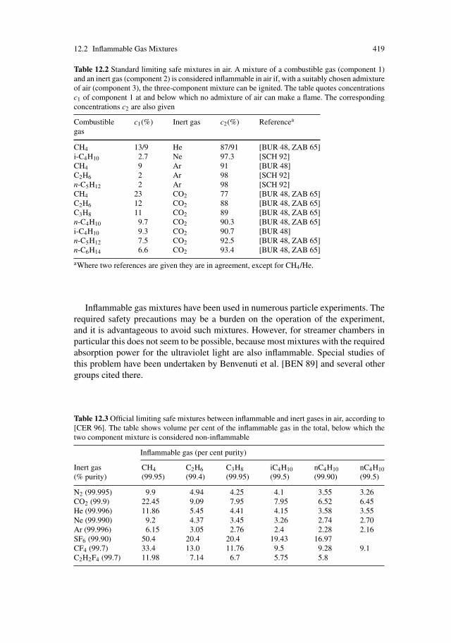
12.2 Inflammable Gas Mixtures 419
Table 12.2 Standard limiting safe mixtures in air. A mixture of a combustible gas (component 1)and an inert gas (component 2) is considered inflammable in air if, with a suitably chosen admixtureof air (component 3), the three-component mixture can be ignited. The table quotes concentrationsc1 of component 1 at and below which no admixture of air can make a flame. The correspondingconcentrations c2 are also given
Combustible c1(%) Inert gas c2(%) Referencea
gas
CH4 13/9 He 87/91 [BUR 48, ZAB 65]i-C4H10 2.7 Ne 97.3 [SCH 92]CH4 9 Ar 91 [BUR 48]C2H6 2 Ar 98 [SCH 92]n-C5H12 2 Ar 98 [SCH 92]CH4 23 CO2 77 [BUR 48, ZAB 65]C2H6 12 CO2 88 [BUR 48, ZAB 65]C3H8 11 CO2 89 [BUR 48, ZAB 65]n-C4H10 9.7 CO2 90.3 [BUR 48, ZAB 65]i-C4H10 9.3 CO2 90.7 [BUR 48]n-C5H12 7.5 CO2 92.5 [BUR 48, ZAB 65]n-C6H14 6.6 CO2 93.4 [BUR 48, ZAB 65]
aWhere two references are given they are in agreement, except for CH4/He.
Inflammable gas mixtures have been used in numerous particle experiments. Therequired safety precautions may be a burden on the operation of the experiment,and it is advantageous to avoid such mixtures. However, for streamer chambers inparticular this does not seem to be possible, because most mixtures with the requiredabsorption power for the ultraviolet light are also inflammable. Special studies ofthis problem have been undertaken by Benvenuti et al. [BEN 89] and several othergroups cited there.
Table 12.3 Official limiting safe mixtures between inflammable and inert gases in air, according to[CER 96]. The table shows volume per cent of the inflammable gas in the total, below which thetwo component mixture is considered non-inflammable
Inflammable gas (per cent purity)
Inert gas CH4 C2H6 C3H8 iC4H10 nC4H10 nC4H10(% purity) (99.95) (99.4) (99.95) (99.5) (99.90) (99.5)
N2 (99.995) 9.9 4.94 4.25 4.1 3.55 3.26CO2 (99.9) 22.45 9.09 7.95 7.95 6.52 6.45He (99.996) 11.86 5.45 4.41 4.15 3.58 3.55Ne (99.990) 9.2 4.37 3.45 3.26 2.74 2.70Ar (99.996) 6.15 3.05 2.76 2.4 2.28 2.16SF6 (99.90) 50.4 20.4 20.4 19.43 16.97CF4 (99.7) 33.4 13.0 11.76 9.5 9.28 9.1C2H2F4 (99.7) 11.98 7.14 6.7 5.75 5.8
420 12 Drift-Chamber Gases
12.3 Gas Purity, and Some Practical Measurementsof Electron Attachment
Together with the gases intended to serve in a chamber, there will always be somecontamination, by impurities in the bottles delivered from industry, from outgassingconstruction materials in the gas stream or produced in operation, or arriving fromthe outside world through membranes that are not entirely tight.
Even minor contamination may have adverse effects on the chamber operation. Itcan change the drift velocity (a drastic example is reported in Sect. 12.3.3), or theymay remove drifting electrons by attachment (see Sects. 12.3.1 and 12.3.2). They area cause of chamber ageing (Sect. 12.6). But they can also have a beneficial effect:ionization tracks produced by pulsed UV lasers often depend on some unknownmolecular compound that happens to be in the chamber gas (cf. Sect. 12.4).
We have described in Chap. 2 various mechanisms of negative-ion formationwhich may lead to a loss of electrons drifting through a chamber. It is chiefly byvarying the partial pressures of two clean gases that the two-body and three-bodyprocesses can be experimentally distinguished. The values reported in Figs. 2.11 and2.12a-d were obtained in this way, mostly by workers engaged in atomic-physicsresearch.
For the purposes of drift chambers it is not always necessary to isolate the exactprocess or to know the electron energy. On the other hand one wants to have electronattachment rates for the multi-component gas mixtures and for drift fields typicalfor applications in particle experiments. We collect here some measurements of thiskind, keeping in mind that the detailed interpretation of the attachment process isnot always required.
12.3.1 Three-Body Attachment to O2, Mediatedby CH4, i-C4H10 and H2O
Electron loss rates were measured in various drift-chamber gases with additions ofoxygen, water or methanol, by Huk, Igo-Kemenes and Wagner [HUK 88].
Working initially at 4 bar with Ar (88%) + CH4 (10%) + i-C4H10 (2%) and withO2 concentrations up to 440 ppm, they varied the total gas pressure and the hydro-carbon and O2 concentrations. They were able to show that the measured electronattenuation rate Rtot associated with oxygen could be understood as a superpositionof rates according to (2.77):
Rtot = ∑Ri ;
Ri = k(i)1 N(O2)N(Xi) ,
where N(O2) is the O2 concentration and the N(Xi) are the concentrations of theother gas components. (The rate proportional to the square of N(O2) is negligible at
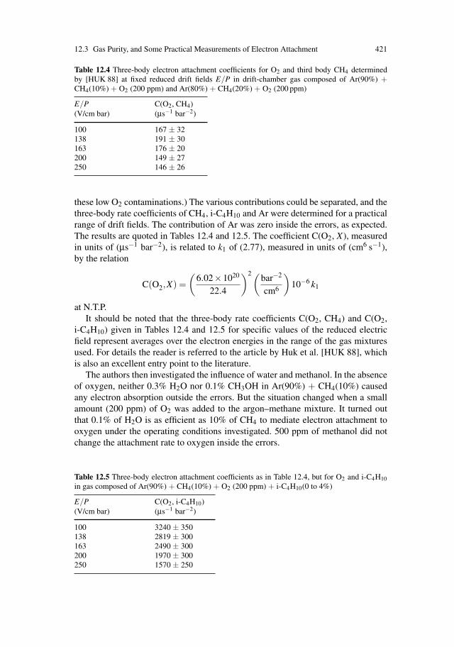
12.3 Gas Purity, and Some Practical Measurements of Electron Attachment 421
Table 12.4 Three-body electron attachment coefficients for O2 and third body CH4 determinedby [HUK 88] at fixed reduced drift fields E/P in drift-chamber gas composed of Ar(90%) +CH4(10%) + O2 (200 ppm) and Ar(80%) + CH4(20%) + O2 (200 ppm)
E/P C(O2, CH4)(V/cm bar) (μs−1 bar−2)
100 167 ± 32138 191 ± 30163 176 ± 20200 149 ± 27250 146 ± 26
these low O2 contaminations.) The various contributions could be separated, and thethree-body rate coefficients of CH4, i-C4H10 and Ar were determined for a practicalrange of drift fields. The contribution of Ar was zero inside the errors, as expected.The results are quoted in Tables 12.4 and 12.5. The coefficient C(O2, X), measuredin units of (μs−1 bar−2), is related to k1 of (2.77), measured in units of (cm6 s−1),by the relation
C(O2,X) =(
6.02×10²⁰
22.4
)2(bar−2
cm6
)10−6 k1
at N.T.P.It should be noted that the three-body rate coefficients C(O2, CH4) and C(O2,
i-C4H10) given in Tables 12.4 and 12.5 for specific values of the reduced electricfield represent averages over the electron energies in the range of the gas mixturesused. For details the reader is referred to the article by Huk et al. [HUK 88], whichis also an excellent entry point to the literature.
The authors then investigated the influence of water and methanol. In the absenceof oxygen, neither 0.3% H2O nor 0.1% CH3OH in Ar(90%) + CH4(10%) causedany electron absorption outside the errors. But the situation changed when a smallamount (200 ppm) of O2 was added to the argon–methane mixture. It turned outthat 0.1% of H2O is as efficient as 10% of CH4 to mediate electron attachment tooxygen under the operating conditions investigated. 500 ppm of methanol did notchange the attachment rate to oxygen inside the errors.
Table 12.5 Three-body electron attachment coefficients as in Table 12.4, but for O2 and i-C4H10in gas composed of Ar(90%) + CH4(10%) + O2 (200 ppm) + i-C4H10(0 to 4%)
E/P C(O2, i-C4H10)(V/cm bar) (μs−1 bar−2)
100 3240 ± 350138 2819 ± 300163 2490 ± 300200 1970 ± 300250 1570 ± 250

422 12 Drift-Chamber Gases
12.3.2 ‘Poisoning’ of the Gas by Construction Materials, CausingElectron Attachment
A long lifetime of electrons, which is essential for the functioning of drift chamberswith long drift paths, is not yet guaranteed when the chamber has been filled withextremely clean gas. The very material of the chamber itself and of its gas distribu-tion system may contaminate the gas with electronegative (i.e. electron-absorbing)impurities which emanate from the surface or the volume of these materials. As wediscussed in Sect. 2.2.7, the two-body attachment rates of some halogen-containingcompounds are so large that even at concentrations as low as 10−8 they willabsorb a sizeable fraction of the electrons that have to drift over a distance ofone metre.
In practice, every piece of material that will come into contact with the gas streamof a long-drift chamber has to be controlled with respect to outgassing before it isbuilt in. Test facilities for this purpose have been in use at Berkeley, CERN andprobably other laboratories. Basically, a long drift tube is connected to a gas distri-bution system which comprises a receptacle for the material in question. In Berkeleythe ‘poisoning time’ Tp was measured for which the test piece has to be in contactwith the 6 m3 of the TPC volume before the attenuation of electrons over 1 m ofdrift increases by 1%. At CERN the results of the measurements were expressed interms of the percentage electron loss A over 1 m of drift after the test piece had beenin contact with 1 m3 of gas for 24 h.
The drift tubes were operated under the conditions of the large chamber thatwas being built in the respective laboratory (PEP-4 TPC at Berkeley: Ar(80%) +CH4(20%) at 10 bar; ALEPH TPC at CERN: Ar(90%) + CH4(10%) at 1 bar; cf.Table 11.4). The results of these technical measurements cannot be directly com-pared because the various contributing 2-body and 3-body attachment rates behavedifferently with respect to gas composition, pressure and electric field.
The results of these tests are documented in two lists [BRO 79] and [LEH 89]containing about a hundred items each. We present in Tables 12.6 and 12.7 someexamples in order to show that many common construction materials do not poisonthe gas, whereas a number of other materials, especially certain cleaning agents,paints and seals, have been found to be disastrous.
12.3.3 The Effect of Minor H2O Contaminationon the Drift Velocity
We present in Fig. 12.5 drift velocities for two argon–methane mixtures, typicalTPC gases, which in addition contain some very low concentrations of water vapour.These measurements from the DELPHI group are basically in agreement with cal-culations of Biagi [BIA 89] and of Schmidt [SCH 86]. Let us note that for some,especially low, values of the electric field, one tenth of a per cent of water vapour
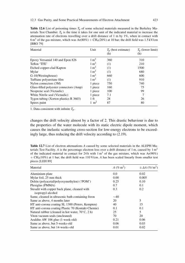
12.3 Gas Purity, and Some Practical Measurements of Electron Attachment 423
Table 12.6 List of poisoning times Tp of some selected materials measured in the Berkeley Ma-terials Test Chamber. Tp is the time it takes for one unit of the indicated material to increase theattenuation rate of electrons travelling over a drift distance of 1 m by 1%, when in contact with6 m3 of the gas mixture, which was Ar(80%) + CH4(20%) at 10 bar; the drift field was 1.5 kV/cm[BRO 79]
Material Unit Tp (best estimate) Tp (lower limit)(h) (h)
Epoxy Versamid 140 and Epon 826 1 m2 360 310Teflon ‘TFE’ 1 m2 (1) 210Etched copper-clad Kapton 1 m2 (1) 1500Mylar 1 m2 (1) 680G-10(Westinghouse) 1 m2 660 600Tufftane polyuretane film 1 m2 (1) 910Nylon connectors (3M) 1 piece 750 740Glass-filled polyester connectors (Amp) 1 piece 160 75Neoprene seal (Victaulic) 1 piece 100 99White Nitrile seal (Victaulic) 1 piece 7.1 7Tygon tubing (Xorton plastics R 3603) 1 ft 28 26Spirex paint 1 m2 87 80
1. Data consistent with infinite Tp.
changes the drift velocity almost by a factor of 2. This drastic behaviour is due tothe properties of the water molecule with its static electric dipole moment, whichcauses the inelastic scattering cross-section for low-energy electrons to be exceed-ingly large, thus reducing the drift velocity according to (2.19).
Table 12.7 List of electron attenuations A caused by some selected materials in the ALEPH Ma-terials Test Facility. A is the percentage electron loss over a drift distance of 1 m, caused by 1 m2
of the indicated material in contact for 24 h with 1 m3 of the gas mixture, which was Ar(90%)+ CH4(10%) at 1 bar; the drift field was 110 V/cm. A has been scaled linearly from smaller testpieces [LEH 89]
Material A (% m2) ±ΔA (%/ m2)
Aluminium plate 0.0 0.02Mylar foil, 25 mm thick 0.00 0.005Delrin (polyacetal/polyoxymethylen) (‘POM’) 0.25 0.10Plexiglas (PMMA) 0.7 0.1Stesalit with copper back plane, cleaned with 0.3 0.2
isopropyl-alcoholSame, cleaned in ultrasonic bath containing freon ∼40Same as above, 4 months later 20 5HT anti-corona coating SL 1300 (Peters, Kempten) 40 15HT anti-corona coating Plastic 70 (Kontakt-Chemie) 0.1 0.1Natural rubber (cleaned in hot water, 70◦C, 2 h) 25 5Viton vacuum seals (uncleaned) 70 20Araldite AW 106 glue (1-week-old) 0.21 0.06Same as above, but 5-weeks-old 0.06 0.03Same as above, but 14-weeks-old 0.01 0.02

424 12 Drift-Chamber Gases
Fig. 12.5a,b Drift velocities measured by [CAT 89] for two argon–methane mixtures containinga small additional amount of water vapour. (a) Ar(91%) + CH4(9%); (b) Ar(80%) + CH4(20%).The measurement errors are estimated to be 1% or less; the lines are drawn to connect the measuredpoints
12.4 Chemical Compounds Used for Laser Ionization
The most often employed technique of creating ionization tracks in the gas of a driftchamber relies on the presence of molecules in the chamber gas that can be ion-ized in a two-step process as discussed in Sect. 1.3. In many chambers the gas hassufficient impurities, owing to the outgassing of materials or as remnants from theproduction process. If the concentration is not large enough for the available laserpower, or if it is not stable, a suitable compound has to be added to the chamber gas.We can look for candidates among the organic vapours with ionization potentialsbelow twice the laser photon energy. A good number of them are known to pro-duce ionizable tracks, but definitive measurements of the second-order cross-sectionequivalent (see Sect. 1.3.1) do not yet exist.
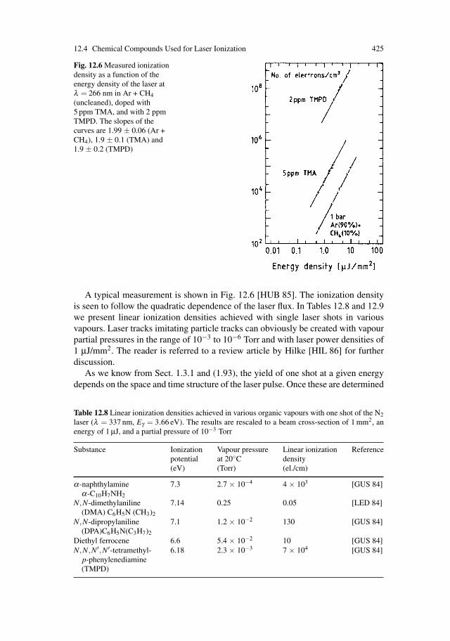
12.4 Chemical Compounds Used for Laser Ionization 425
Fig. 12.6 Measured ionizationdensity as a function of theenergy density of the laser atλ = 266 nm in Ar + CH4(uncleaned), doped with5 ppm TMA, and with 2 ppmTMPD. The slopes of thecurves are 1.99 ± 0.06 (Ar +CH4), 1.9 ± 0.1 (TMA) and1.9 ± 0.2 (TMPD)
A typical measurement is shown in Fig. 12.6 [HUB 85]. The ionization densityis seen to follow the quadratic dependence of the laser flux. In Tables 12.8 and 12.9we present linear ionization densities achieved with single laser shots in variousvapours. Laser tracks imitating particle tracks can obviously be created with vapourpartial pressures in the range of 10−3 to 10−6 Torr and with laser power densities of1 μJ/mm2. The reader is referred to a review article by Hilke [HIL 86] for furtherdiscussion.
As we know from Sect. 1.3.1 and (1.93), the yield of one shot at a given energydepends on the space and time structure of the laser pulse. Once these are determined
Table 12.8 Linear ionization densities achieved in various organic vapours with one shot of the N2laser (λ = 337 nm, Eγ = 3.66 eV). The results are rescaled to a beam cross-section of 1 mm2, anenergy of 1 μJ, and a partial pressure of 10−3 Torr
Substance Ionization Vapour pressure Linear ionization Referencepotential at 20◦C density(eV) (Torr) (el./cm)
α-naphthylamine 7.3 2.7 × 10⁻⁴ 4 × 10³ [GUS 84]α-C10H7NH2
N,N-dimethylaniline 7.14 0.25 0.05 [LED 84](DMA) C6H5N (CH3)2
N,N-dipropylaniline 7.1 1.2 × 10⁻² 130 [GUS 84](DPA)C6H5N(C3H7)2
Diethyl ferrocene 6.6 5.4 × 10⁻² 10 [GUS 84]N,N,N′,N′-tetramethyl- 6.18 2.3 × 10⁻³ 7 × 10⁴ [GUS 84]
p-phenylenediamine(TMPD)
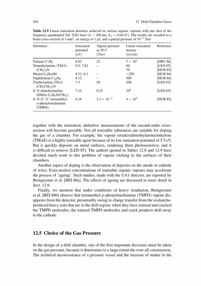
426 12 Drift-Chamber Gases
Table 12.9 Linear ionization densities achieved in various organic vapours with one shot of thefrequency-quadrupled Nd: YAG laser (λ = 266 nm, Eγ = 4.64 eV). The results are rescaled to abeam cross-section of 1 mm2, an energy of 1 μJ, and a partial pressure of 10−3 Torr
Substance Ionization Vapour pressure Linear ionization Referencepotential at 20◦C density(eV) (Torr) (el./cm)
Toluene C7H8 8.82 22 7 × 10³ [DRY 86]Trimethylamine (TMA) 8.5; 7.82 – 60 [LED 85]
(CH3)3N 70 [HUB 85]Phenol C6H5OH 8.51; 8.3 – >250 [HUB 86]Naphthalene C10H8 8.12 – 500 [HUB 86]Triethylamine (TEA) 7.5 50 200 [LED 85]
(CH3CH2)3NN,N-dimethylaniline 7.14 0.25 104 [LED 85]
(DMA) C6H5N(CH3)2
N,N,N′,N’-tetramethyl- 6.18 2.3 × 10⁻³ 4 × 10⁴ [HUB 85]p-phenylenediamine(TMPD)
together with the ionization, definitive measurements of the second-order cross-section will become possible. Not all ionizable substances are suitable for dopingthe gas of a chamber. For example, the vapour tetrakis(dimethylamine)ethylene(TMAE) is a highly ionizable agent because of its low ionization potential of 5.5 eV.But it quickly deposits on metal surfaces, rendering them photosensitive, and itis difficult to remove [LED 85]. The authors quoted in Tables 12.8 and 12.9 havedevoted much work to this problem of vapour sticking to the surfaces of theirchambers.
Another aspect of doping is the observation of deposits on the anode or cathodeof wires. Even modest concentrations of ionizable organic vapours may acceleratethe process of ‘ageing’. Such studies, made with the UA1 detector, are reported byBeingessner et al. [BEI 88a]. The effects of ageing are discussed in more detail inSect. 12.6.
Finally, we mention that under conditions of heavy irradiation, Beingessneret al. [BEI 88b] observe that tetramethyl-p-phenylenediamine (TMPD) vapour dis-appears from the detector, presumably owing to charge transfer from the avalanche-produced heavy ions that are in the drift region; when they have ionized and crackedthe TMPD molecules, the ionized TMPD molecules and crack products drift awayto the cathode.
12.5 Choice of the Gas Pressure
In the design of a drift chamber, one of the first important decisions must be takenon the gas pressure, because it determines to a large extent the over-all construction.The technical inconvenience of a pressure vessel and the increase of matter in the

12.5 Choice of the Gas Pressure 427
path of the particles are balanced to a certain degree by some advantages in themeasuring accuracy, and we want to review them here. We note in passing that thewall thickness of a vessel must increase in proportion to the over-pressure it hasto hold.
We have stated in (2.85) that for the mobility tensor the electric and magneticfields scale with the gas density. One would therefore like to discuss the gas densityalways in connection with the corresponding change of the electric and magneticfield strengths, thus keeping the drift-velocity vector constant. But in practice an in-crease of the relevant field strength is easy in the electric and difficult in the magneticcase. Therefore, we proceed by specifying the magnetic field first, the gas density isdiscussed next, and then the electric fields are adjusted accordingly. The gas densityis varied by changing the pressure, since one usually works at room temperature.
Let us consider the various consequences of a change of the gas pressure by afactor p > 1, say from 1 bar to p bar. Table 12.10 contains a summary of the mostimportant effects.
12.5.1 Point-Measuring Accuracy
In measurement accuracy, insofar as it is limited by diffusion, one gains by increas-ing the pressure – unless the limitation is in the diffusion transverse to the magneticfield, and ωτ � 1. Therefore, we distinguish between the following:
(a) Longitudinal diffusion or ωτ 1: For the width of the diffusion cloud onegains a factor l/
√p (2.61, 63), and in the accuracy to find the centre of the
cloud one gains another factor 1/√
p, because the statistical fluctuations varywith 1/
√Ntot, where Ntot is the total number of electrons in the diffusion cloud.
Therefore, the over-all gain is a factor 1/p.(b) Transverse diffusion with ωτ � 1: For the width of the diffusion cloud one
loses a factor√
p according to (2.61, 63, 72). The statistical fluctuations com-pensate this; therefore, the over-all factor is 1.
The contributions to the measurement accuracy that arise from the driftpath varia-tions have statistical fluctuations that vary with 1/
√Neff (see (1.73) and Sect. 7.2.3).
As the pressure is increased, Neff increases as well, but only slowly. For the purposeof the present estimates we take Neff proportional to
√p (Figs. 1.22 and 1.23). The
situation would change where declustering occurred in any important measure. Thedrift-path variations are partly due to the wire geometry, i.e. constant when p varies,but partly they have a pressure dependence of their own. This is the case for the wireE ×B effect. Here we refer to the angle at which the electrons approach the wires intheir immediate neighbourhood (Sect. 7.3.1). The tangent of the effective Lorentzangle ψ will decrease roughly proportional to 1/p, as p increases. A smaller angleψ will reduce the drift-path variations. Depending on how important the wire E ×Beffect is in comparison to the other drift-path variations, we may say in summarythat the contributions to the measurement accuracy that arise from the drift-pathvariations decrease as a function of p which is somewhere between 1/p and 1/p0.25.
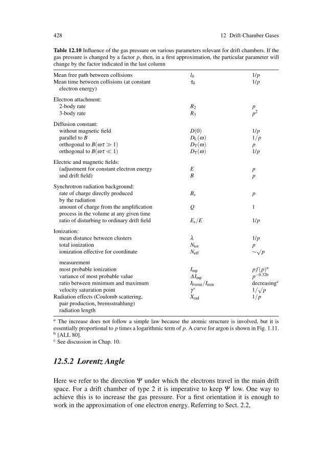
428 12 Drift-Chamber Gases
Table 12.10 Influence of the gas pressure on various parameters relevant for drift chambers. If thegas pressure is changed by a factor p, then, in a first approximation, the particular parameter willchange by the factor indicated in the last column
Mean free path between collisions l0 1/pMean time between collisions (at constant τ0 1/p
electron energy)
Electron attachment:2-body rate R2 p3-body rate R3 p2
Diffusion constant:without magnetic field D(0) 1/pparallel to B DL(ω) 1/porthogonal to B(ωτ � 1) DT(ω) porthogonal to B(ωτ 1) DT(ω) 1/p
Electric and magnetic fields:(adjustment for constant electron energy E pand drift field) B p
Synchrotron radiation background:rate of charge directly produced Bs pby the radiationamount of charge from the amplification Q 1process in the volume at any given timeratio of disturbing to ordinary drift field Es/E 1/p
Ionization:mean distance between clusters λ 1/ptotal ionization Ntot pionization effective for coordinate Neff ∼√
p
measurementmost probable ionization Imp p f (p)a
variance of most probable value Δ Imp p−0.32b
ratio between minimum and maximum IFermi/Imin decreasingc
velocity saturation point γ∗ 1/√
pRadiation effects (Coulomb scattering, Xrad 1/p
pair production, bremsstrahlung)radiation length
a The increase does not follow a simple law because the atomic structure is involved, but it isessentially proportional to p times a logarithmic term of p. A curve for argon is shown in Fig. 1.11.b [ALL 80].c See discussion in Chap. 10.
12.5.2 Lorentz Angle
Here we refer to the direction Ψ under which the electrons travel in the main driftspace. For a drift chamber of type 2 it is imperative to keep Ψ low. One way toachieve this is to increase the gas pressure. For a first orientation it is enough towork in the approximation of one electron energy. Referring to Sect. 2.2,
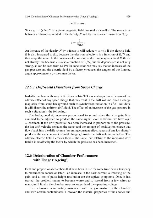
12.6 Deterioration of Chamber Performance with Usage (‘Ageing’) 429
tanΨ = ωτ .
Since ωτ = (e/m)B, at a given magnetic field one seeks a small τ . The mean timebetween collisions is related to the density N and the collision cross-section σ by
τ =1
Nσc.
An increase of the density N by a factor p will reduce τ to τ/p if the electric fieldE is also increased to E p, because the electron velocity c is a function of E/N andthen stays the same. In the presence of a constant and strong magnetic field B, this isnot strictly true because c is also a function of B/N, but the dependence is not verystrong, as can be seen from (2.49). In conclusion we may say that an increase of thegas pressure and the electric field by a factor p reduces the tangent of the Lorentzangle approximately by the same factor.
12.5.3 Drift-Field Distortions from Space Charge
In drift chambers with long drift distances like TPCs one always has to beware of theadverse effect of any space charge that may exist in the drift volume. Such a chargemay arise from some background such as synchrotron radiation in e+e− colliders.It will distort the uniform drift field. The effect of an increase of the gas pressure insuch a situation is the following.
The background Bs increases proportional to p, and since the wire gain G isassumed to be adjusted to produce the same signal level as before, we have BsG= constant. If the drift potential has been increased in proportion to the pressure,the ion drift velocity remains the same, and the amount of positive ion charge thatflows back into the drift volume (assuming constant effectiveness of any ion shutter)produces the same amount of total charge Q inside the drift volume as before. Theadverse electric field it creates there is the same, but relative to the increased driftfield it is smaller by the factor by which the pressure has been increased.
12.6 Deterioration of Chamber Performancewith Usage (‘Ageing’)
Drift and proportional chambers that have been in use for some time have a tendencyto malfunction sooner or later – an increase in the dark current, a lowering of thegain, and a loss of pulse-height resolution are the typical symptoms. Once it hasstarted, the problem seems to become worse and to spread from a few wires tomany, until finally the chamber may no longer hold the operating voltage.
This behaviour is intimately associated with the gas mixture in the chamberand with certain contaminants. However, the material properties of the anodes and

430 12 Drift-Chamber Gases
cathodes as well as their size also play a role in this area which is far from beingclearly understood. Given the practical importance of the subject and that the newaccelerators will produce extremely high levels of radiation, efforts towards betterunderstanding are under way. Workshops held at Berkeley [WOR 86] and Hamburg[WOR 01] summarized the experience. A comparison of the reports at the two pro-ceedings shows that during the 15 years between them there was much progresstowards mastering the high particle fluxes of modern times. On the other hand, thereis still no fundamental understanding of ageing. Nobody can calculate the lifetimeof a chamber to be built, and in most cases one cannot even calculate what the re-sult will be when some parameter is changed in a given chamber and its gas supplysystem.
12.6.1 General Observations in Particle Experiments
The wires of degraded chambers carry deposits of various kinds, either as spotsor as complete coatings of the anode or cathode wires, smooth or hairy, white orblack or oily, in the region of the strongest exposure. One quantifies the lifetimeof a wire by adding up the charge that it has collected during its lifetime; it iscalculated as the total charge that has drifted towards it times the avalanche gain.Lifetimes at which performance losses have been reported are in the range 10−4 −1Coulomb per cm of wire length. It appears that the lower limit of 10−4C/cm hasbecome rather uncommon since the problems with the particular gas mixture con-sisting of Ar (75%), isobutane (24.5%), and freon (0.5%) have become understood[SAU 86]. (This mixture was employed in the very first proportional chamber sys-tems and, among experts, went under the name ‘magic gas’; it was used for very highavalanche gain factors beyond the proportional mode.) Most often, lifetimes are re-ported to be above 10−2C/cm before deterioration sets in. With special precautionssuch lifetimes may be extended by an order of magnitude or more. Table 12.11 con-tains a collection of particle experiments with details about the behaviour of ageingchambers and some special precautions.
12.6.2 Dark Currents
The build up of a dark current drawn by the anode wire of a deteriorated chambereven in the absence of radiation can be explained by the ‘thin-field emission effect’,or Malter effect [MAL 36]. In his experiment, Malter showed that a positive surfacecharge deposited on a thin insulating film that covers a cathode can provoke theemission of electrons from the cathode through the film. A very high electric fieldmay be created in the film between the deposited charge and the counterchargesaccumulated on the metallic cathode on the opposite side. Electrons are extractedfrom the metal through field emission and may find their way through the film into

12.6 Deterioration of Chamber Performance with Usage (‘Ageing’) 431
Table 12.11 Drift and proportional chambers exposed to high radiation doses – reports of someaccelerator experiments with high densities of accumulated charge
Chamber Reference Basic gas Additional Accumulated Observedmixture measures charge density effectsa
(percentages) (concentrations (C/cm)in %)
TASSO central [BIN 86] Ar(50) C2H5OH (1.6) 0.2–0.4 Nonedetector +C2H6(50) + oil in ethane
removed gasfilters inserted
TASSO vertex [BIN 86] Ar(95)+CO2(5) H2O(1) 0.25 Somechamber +C2H5OH
(0.12)(3 bar)Split field [ULL 86] Ar(53) – 0.3 Anode wire
magnet +i-C4H10(40) coating,chambers +(CH2OH)2 thickness 1 μm
CH2(7)
ACCMOR drift [TUR 86] Ar(50) (CH3)2 0.02 Nonechambers +C2H6(50) CHOH(0.2)
Ar(60)+C2H6
(40)
ARGUS drift [DAN 89] C3H8(97) H2O(0.2) 0.005 Nonechamber +(CH2OH)2
CH2(3)BNL hyper- [PIL 86] Ar(50) covering soft 0.2 None
nuclear spec- +C2H6(50) urethanetrometer adhesiveDC
FNAL tagged [EST 86] Ar(50) C2H5OH 0.1–0.2 Efficiency lossphoton spec- C2H6(50) wire cleaningrometer
UA1 central [YVE 86] Ar(40) – 0.01 Nonechamber +C2H6(60)
Argonne ZGS [SPI 86] Ar(65) new bubbler oil, 0.1–1 Efficiency loss,beam chambers +CO2(35) new plastic tubes, deposits (Si)
+CBrF3 new wires on anodes,(0.5) cathodes
EMC muon [HIL 86] Ar(79.5) – 0.15 Anode deposits,chambers +CH4(19.5) efficiency loss
30%after 0.25: End of
operation
J-Spectrometer, [BEC 92] [Ar+ – 0.1–1 Deposits on flatBNL (1974), front (CH2OH)2 cathode,proportional CH2](0◦C)b chamberschambers still efficient
aAfter the additional measuresbArgon saturated with methylal at 0◦C
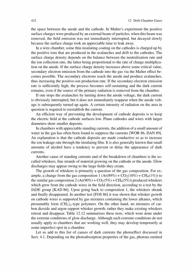
432 12 Drift-Chamber Gases
the space between the anode and the cathode. In Malter’s experiment the positivesurface charges were produced by an external beam of particles; when this beam wasremoved, the field emission was not immediately interrupted, but decayed slowlybecause the surface charge took an appreciable time to leak away.
In a wire chamber, some thin insulating coating on the cathodes is charged up bythe positive ions that are produced in the avalanches and drift to the cathodes. Thesurface charge density depends on the balance between the neutralisation rate andthe ion collection rate, the latter being proportional to the rate of charge multiplica-tion on the anode. If the surface charge density increases above some critical value,secondary electron emission from the cathode into the gas via the Malter effect be-comes possible. The secondary electrons reach the anode and produce avalanches,thus increasing the positive-ion production rate. If the secondary-electron emissionrate is sufficiently high, the process becomes self-sustaining and the dark currentremains, even if the source of the primary radiation is removed from the chamber.
If one stops the avalanches by turning down the anode voltage, the dark currentis obviously interrupted, but it does not immediately reappear when the anode volt-age is subsequently turned up again. A certain intensity of radiation on the area inquestion is required to reestablish the current.
An efficient way of preventing the development of cathode deposits is to keepthe electric field at the cathode surfaces low. Plane cathodes and wires with largerdiameters show smaller deposits.
In chambers with appreciable standing currents, the addition of a small amount ofwater in the gas has often been found to suppress the currents [WOR 86, DAN 89].An explanation is that the cathode deposits are made conductive so as to increasethe ion leakage rate through the insulating film. It is also generally known that smallamounts of alcohol have a tendency to prevent or delay the appearance of darkcurrents.
Another cause of standing currents and of the breakdown of chambers is the so-called whiskers, fine strands of material growing on the cathode or the anode. Glowdischarges may appear owing to the large fields they create.
The growth of whiskers is primarily a question of the gas composition. For ex-ample, a change from the gas composition 1 (Ar(89%) + CO2(10%) + CH4(1%)) tothe similar gas composition 2 (Ar(90%) + CO2(5%) + CH4(5%)) produced whiskerswhich grew from the cathode wires in the field direction, according to a test by theJADE group [KAD 86]. Upon going back to composition 1, the whiskers shrankand finally disappeared. In another test [FOS 86] it was shown that whisker growthon cathode wires is supported by gas mixtures containing the lower alkanes, whichpresumably form (CH2)n-type polymers. On the other hand, no mixtures of car-bon dioxide and argon support whisker growth; rather they make existing whiskersretreat and disappear. Table 12.12 summarises these tests, which were done underthe extreme conditions of glow discharge. Although such extreme conditions do notusually apply to chambers that are working well, they may develop temporarily atsome imperfect spot in a chamber.
Let us add to this list of causes of dark currents the photoeffect discussed inSect. 4.1. Depending on the photoabsorption properties of the gas, photons emitted
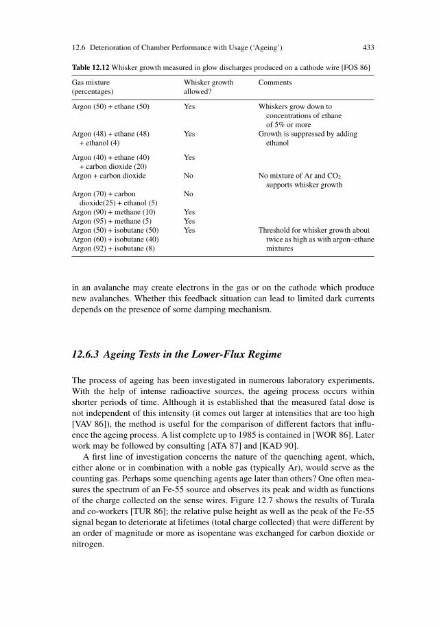
12.6 Deterioration of Chamber Performance with Usage (‘Ageing’) 433
Table 12.12 Whisker growth measured in glow discharges produced on a cathode wire [FOS 86]
Gas mixture Whisker growth Comments(percentages) allowed?
Argon (50) + ethane (50) Yes Whiskers grow down toconcentrations of ethaneof 5% or more
Argon (48) + ethane (48) Yes Growth is suppressed by adding+ ethanol (4) ethanol
Argon (40) + ethane (40) Yes+ carbon dioxide (20)
Argon + carbon dioxide No No mixture of Ar and CO2supports whisker growth
Argon (70) + carbon Nodioxide(25) + ethanol (5)
Argon (90) + methane (10) YesArgon (95) + methane (5) YesArgon (50) + isobutane (50) Yes Threshold for whisker growth aboutArgon (60) + isobutane (40) twice as high as with argon–ethaneArgon (92) + isobutane (8) mixtures
in an avalanche may create electrons in the gas or on the cathode which producenew avalanches. Whether this feedback situation can lead to limited dark currentsdepends on the presence of some damping mechanism.
12.6.3 Ageing Tests in the Lower-Flux Regime
The process of ageing has been investigated in numerous laboratory experiments.With the help of intense radioactive sources, the ageing process occurs withinshorter periods of time. Although it is established that the measured fatal dose isnot independent of this intensity (it comes out larger at intensities that are too high[VAV 86]), the method is useful for the comparison of different factors that influ-ence the ageing process. A list complete up to 1985 is contained in [WOR 86]. Laterwork may be followed by consulting [ATA 87] and [KAD 90].
A first line of investigation concerns the nature of the quenching agent, which,either alone or in combination with a noble gas (typically Ar), would serve as thecounting gas. Perhaps some quenching agents age later than others? One often mea-sures the spectrum of an Fe-55 source and observes its peak and width as functionsof the charge collected on the sense wires. Figure 12.7 shows the results of Turalaand co-workers [TUR 86]; the relative pulse height as well as the peak of the Fe-55signal began to deteriorate at lifetimes (total charge collected) that were different byan order of magnitude or more as isopentane was exchanged for carbon dioxide ornitrogen.
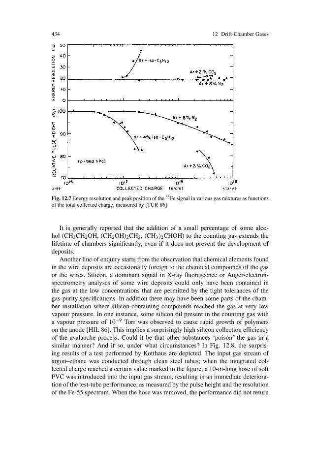
434 12 Drift-Chamber Gases
Fig. 12.7 Energy resolution and peak position of the 55Fe signal in various gas mixtures as functionsof the total collected charge, measured by [TUR 86]
It is generally reported that the addition of a small percentage of some alco-hol (CH3CH2OH, (CH2OH)2CH2, (CH3)2CHOH) to the counting gas extends thelifetime of chambers significantly, even if it does not prevent the development ofdeposits.
Another line of enquiry starts from the observation that chemical elements foundin the wire deposits are occasionally foreign to the chemical compounds of the gasor the wires. Silicon, a dominant signal in X-ray fluorescence or Auger-electron-spectrometry analyses of some wire deposits could only have been contained inthe gas at the low concentrations that are permitted by the tight tolerances of thegas-purity specifications. In addition there may have been some parts of the cham-ber installation where silicon-containing compounds reached the gas at very lowvapour pressure. In one instance, some silicon oil present in the counting gas witha vapour pressure of 10−9 Torr was observed to cause rapid growth of polymerson the anode [HIL 86]. This implies a surprisingly high silicon collection efficiencyof the avalanche process. Could it be that other substances ‘poison’ the gas in asimilar manner? And if so, under what circumstances? In Fig. 12.8, the surpris-ing results of a test performed by Kotthaus are depicted. The input gas stream ofargon–ethane was conducted through clean steel tubes; when the integrated col-lected charge reached a certain value marked in the figure, a 10-m-long hose of softPVC was introduced into the input gas stream, resulting in an immediate deteriora-tion of the test-tube performance, as measured by the pulse height and the resolutionof the Fe-55 spectrum. When the hose was removed, the performance did not return
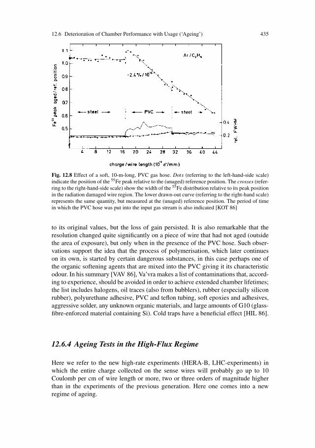
12.6 Deterioration of Chamber Performance with Usage (‘Ageing’) 435
Fig. 12.8 Effect of a soft, 10-m-long, PVC gas hose. Dots (referring to the left-hand-side scale)indicate the position of the 55Fe peak relative to the (unaged) reference position. The crosses (refer-ring to the right-hand-side scale) show the width of the 55Fe distribution relative to its peak positionin the radiation damaged wire region. The lower drawn-out curve (referring to the right-hand scale)represents the same quantity, but measured at the (unaged) reference position. The period of timein which the PVC hose was put into the input gas stream is also indicated [KOT 86]
to its original values, but the loss of gain persisted. It is also remarkable that theresolution changed quite significantly on a piece of wire that had not aged (outsidethe area of exposure), but only when in the presence of the PVC hose. Such obser-vations support the idea that the process of polymerisation, which later continueson its own, is started by certain dangerous substances, in this case perhaps one ofthe organic softening agents that are mixed into the PVC giving it its characteristicodour. In his summary [VAV 86], Va’vra makes a list of contaminations that, accord-ing to experience, should be avoided in order to achieve extended chamber lifetimes;the list includes halogens, oil traces (also from bubblers), rubber (especially siliconrubber), polyurethane adhesive, PVC and teflon tubing, soft epoxies and adhesives,aggressive solder, any unknown organic materials, and large amounts of G10 (glass-fibre-enforced material containing Si). Cold traps have a beneficial effect [HIL 86].
12.6.4 Ageing Tests in the High-Flux Regime
Here we refer to the new high-rate experiments (HERA-B, LHC-experiments) inwhich the entire charge collected on the sense wires will probably go up to 10Coulomb per cm of wire length or more, two or three orders of magnitude higherthan in the experiments of the previous generation. Here one comes into a newregime of ageing.
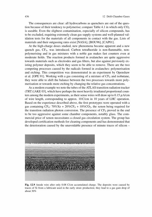
436 12 Drift-Chamber Gases
The consequences are clear: all hydrocarbons as quenchers are out of the ques-tion because of their tendency to polymerise; compare Table 4.1 in which only CO2
is useable. Even the slightest contamination, especially of silicon compounds, hasto be excluded, requiring extremely clean gas supply systems and well-planned val-idation tests for the materials of all components in contact with the gas. Lists ofmaterials and their outgassing rates exist [NASA], [BOU96], [CAP01].
At the high-charge doses studied, new phenomena became apparent and a newquench gas, CF4, was introduced. Carbon tetrafluoride is non-flammable, non-polymerising and in gas mixtures with a noble gas makes fast counters even atmoderate fields. The reaction products formed in avalanches are quite aggressivetowards materials such as electrodes and gas filters, but also against previously ex-isting polymer deposits, which they seem to be able to remove. There are the twocompeting processes caused by the radicals formed in avalanches: polymerisationand etching. This competition was demonstrated in an experiment by Openshawet al. [OPE 91]. Working with a gas consisting of a mixture of CF4 and isobutane,they were able to shift the balance between the two processes towards more poly-merisation or towards more etching by changing the relative gas concentrations.
As a modern example we note the tubes of the ATLAS transition radiation tracker(TRT) [AKE 03], which have perhaps the most heavily irradiated proportional coun-ters among the modern experiments, as their sense wires will draw up to 0.15 μA/cmof wire length, corresponding to approx. 10 C/cm in 10 years of LHC operation.Based on the experience described above, the first prototypes were operated with agas containing CF4: 70%Xe + 20%CF4 + 10%CO2, the xenon being required forthe transition radiation photon conversion. The presence of CF4 proved in the endto be too aggressive against some chamber components, notably glass. The com-mercial price of xenon necessitates a closed gas circulation system. The group hasdeveloped certification methods for cleaning components and has demonstrated thatthe deterioration caused by the unavoidable presence of minute traces of silicon –
Fig. 12.9 Anode wire after only 0.08 C/cm accumulated charge. The deposits were caused bytraces of Si from a lubricant used in the early straw production; they lead to a gas gain drop ofabout 30%
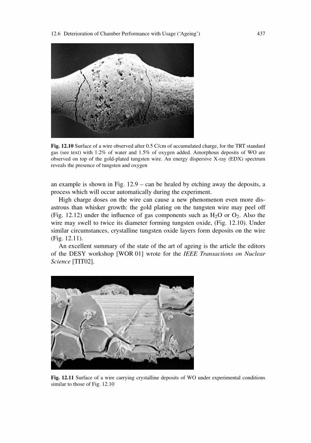
12.6 Deterioration of Chamber Performance with Usage (‘Ageing’) 437
Fig. 12.10 Surface of a wire observed after 0.5 C/cm of accumulated charge, for the TRT standardgas (see text) with 1.2% of water and 1.5% of oxygen added. Amorphous deposits of WO areobserved on top of the gold-plated tungsten wire. An energy dispersive X-ray (EDX) spectrumreveals the presence of tungsten and oxygen
an example is shown in Fig. 12.9 – can be healed by etching away the deposits, aprocess which will occur automatically during the experiment.
High charge doses on the wire can cause a new phenomenon even more dis-astrous than whisker growth: the gold plating on the tungsten wire may peel off(Fig. 12.12) under the influence of gas components such as H2O or O2. Also thewire may swell to twice its diameter forming tungsten oxide, (Fig. 12.10). Undersimilar circumstances, crystalline tungsten oxide layers form deposits on the wire(Fig. 12.11).
An excellent summary of the state of the art of ageing is the article the editorsof the DESY workshop [WOR 01] wrote for the IEEE Transactions on NuclearScience [TIT02].
Fig. 12.11 Surface of a wire carrying crystalline deposits of WO under experimental conditionssimilar to those of Fig. 12.10

438 12 Drift-Chamber Gases
Fig. 12.12 Various manifestations of damage to the gold-plating after 2-6 C/cm of accumulatedcharge for diffferent current densities (1-4 μA/cm). No gold-plating damage was observed whenthe water content was below 0.1%. All photographs from [AKE 03]

References 439
The requirement to eliminate all hydrocarbons from the gas of proportionalchambers dedicated to very-high-rate experiments changes the situation in a drasticway. Whereas previously we carefully optimised the gas properties by choosing theright gas composition from a good variety of possible components, now there areonly a few left. Important gas properties such as the drift velocity and its depen-dence on electric and magnetic fields, diffusion, Lorentz angle, quenching strength,etc. (cf. Sects. 12.1, 12.5) must be taken as they come, if the chambers are to sur-vive the high dose awaiting them in the new experiments. If, for example, the driftvelocity cannot be made insensitive to the electric field, any space charge in the driftregion will limit the measurement accuracy and open a new frontier for the controland, perhaps, correction of such effects.
A thorough understanding of the ageing process must involve the chemicalprocesses in the plasma of the avalanches. There are certainly several competingmechanisms at work; this is also apparent from the wide variety of manifestationsof the deposits as well as from the fact that drastically different element abundancesare measured in different spots along the wires [KOT 86].
At present we do not even know whether a better understanding of the plasmapolymerisation on our wires will give us the means to substantially prolong thelifetime of the chambers. Thus for the time being we are left with a few rules –to keep the gas and the wires extremely clean, to add some alcohol or water ifnecessary, and to keep the cathode wires thick. Since it is the total collected chargewhich destroys the wire, it is useful to keep the amplification low.
References
[AKE 03] T. Akeson et al., Aging studies for the ATLAS Transition Radiation Tracker (TRT),in [WOR01], p. 166
[ATA 87] M. Atac, Wire chamber aging and wire material, IEEE Trans. NS 34, 476 (1987)[BEC 92] U. Becker, private communication (1992)[BEI 88a] S.P. Beingessner, T.C. Meyer and M. Yvert, Influence of chemical trace additives on
the future ageing of the UA1 central detector, Nucl. Instrum. Methods A 272, 669(1988)
[BEI 88b] S.P. Beingessner, T.C. Meyer, A. Norton, M. Pimia, C. Rubbia and V. Vuillemin, Firstrunning experience with the laser calibration system of the UA1 central detector, inProc. Int. Conf. on Advanced Technology and Particle Physics, Villa Olmo (Como),Italy, 1988
[BEN 89] A.C. Benvenuti et al., A nonflammable gas mixture for plastic limited streamer tubes.Nucl. Instrum. Methods Phys. Res. A 284, 339 (1989)
[BIA 89] S.F. Biagi, A multiterm Boltzmann analysis of drift velocity, diffusion, gain and mag-netic effects in argon-methane-water-vapour mixtures, Nucl. Instrum. Methods Phys.Res. A 283, 716 (1989)
[BIN 86] D.M. Binnie, Experience with the TASSO chambers, in [WOR 86], p. 213[BOU96] R. Bouclier et al., xxxx, Nucl. Instrum. Methods A 381, 289 (1996)[BRE 74] A. Breskin, G. Charpak, B. Gabioud, F. Sauli, N. Trautner, W. Duinker, G. Schultz,
Further results on the operation of high-accuracy drift chambers, Nucl. Instrum.Methods 119, 9 (1974)
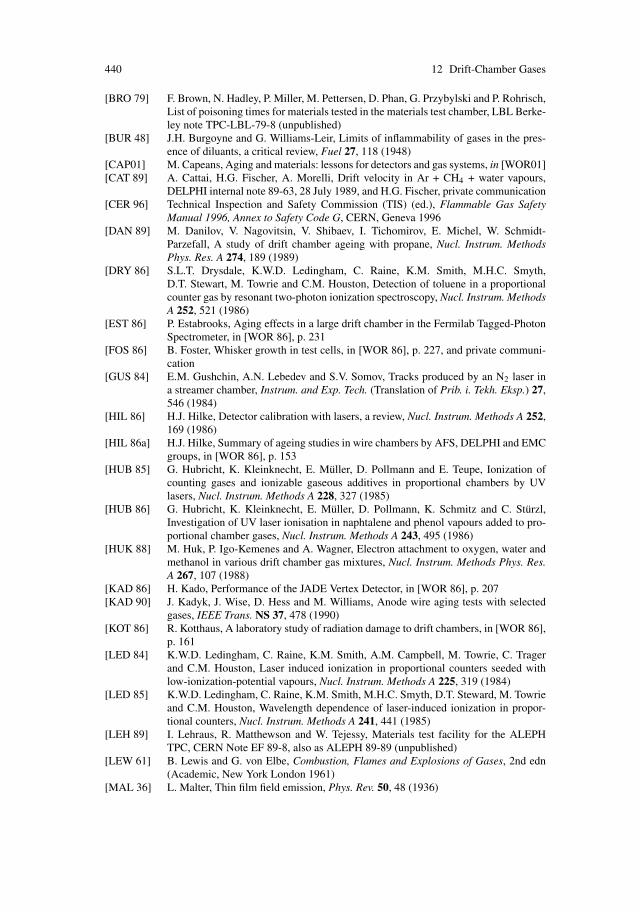
440 12 Drift-Chamber Gases
[BRO 79] F. Brown, N. Hadley, P. Miller, M. Pettersen, D. Phan, G. Przybylski and P. Rohrisch,List of poisoning times for materials tested in the materials test chamber, LBL Berke-ley note TPC-LBL-79-8 (unpublished)
[BUR 48] J.H. Burgoyne and G. Williams-Leir, Limits of inflammability of gases in the pres-ence of diluants, a critical review, Fuel 27, 118 (1948)
[CAP01] M. Capeans, Aging and materials: lessons for detectors and gas systems, in [WOR01][CAT 89] A. Cattai, H.G. Fischer, A. Morelli, Drift velocity in Ar + CH4 + water vapours,
DELPHI internal note 89-63, 28 July 1989, and H.G. Fischer, private communication[CER 96] Technical Inspection and Safety Commission (TIS) (ed.), Flammable Gas Safety
Manual 1996, Annex to Safety Code G, CERN, Geneva 1996[DAN 89] M. Danilov, V. Nagovitsin, V. Shibaev, I. Tichomirov, E. Michel, W. Schmidt-
Parzefall, A study of drift chamber ageing with propane, Nucl. Instrum. MethodsPhys. Res. A 274, 189 (1989)
[DRY 86] S.L.T. Drysdale, K.W.D. Ledingham, C. Raine, K.M. Smith, M.H.C. Smyth,D.T. Stewart, M. Towrie and C.M. Houston, Detection of toluene in a proportionalcounter gas by resonant two-photon ionization spectroscopy, Nucl. Instrum. MethodsA 252, 521 (1986)
[EST 86] P. Estabrooks, Aging effects in a large drift chamber in the Fermilab Tagged-PhotonSpectrometer, in [WOR 86], p. 231
[FOS 86] B. Foster, Whisker growth in test cells, in [WOR 86], p. 227, and private communi-cation
[GUS 84] E.M. Gushchin, A.N. Lebedev and S.V. Somov, Tracks produced by an N2 laser ina streamer chamber, Instrum. and Exp. Tech. (Translation of Prib. i. Tekh. Eksp.) 27,546 (1984)
[HIL 86] H.J. Hilke, Detector calibration with lasers, a review, Nucl. Instrum. Methods A 252,169 (1986)
[HIL 86a] H.J. Hilke, Summary of ageing studies in wire chambers by AFS, DELPHI and EMCgroups, in [WOR 86], p. 153
[HUB 85] G. Hubricht, K. Kleinknecht, E. Muller, D. Pollmann and E. Teupe, Ionization ofcounting gases and ionizable gaseous additives in proportional chambers by UVlasers, Nucl. Instrum. Methods A 228, 327 (1985)
[HUB 86] G. Hubricht, K. Kleinknecht, E. Muller, D. Pollmann, K. Schmitz and C. Sturzl,Investigation of UV laser ionisation in naphtalene and phenol vapours added to pro-portional chamber gases, Nucl. Instrum. Methods A 243, 495 (1986)
[HUK 88] M. Huk, P. Igo-Kemenes and A. Wagner, Electron attachment to oxygen, water andmethanol in various drift chamber gas mixtures, Nucl. Instrum. Methods Phys. Res.A 267, 107 (1988)
[KAD 86] H. Kado, Performance of the JADE Vertex Detector, in [WOR 86], p. 207[KAD 90] J. Kadyk, J. Wise, D. Hess and M. Williams, Anode wire aging tests with selected
gases, IEEE Trans. NS 37, 478 (1990)[KOT 86] R. Kotthaus, A laboratory study of radiation damage to drift chambers, in [WOR 86],
p. 161[LED 84] K.W.D. Ledingham, C. Raine, K.M. Smith, A.M. Campbell, M. Towrie, C. Trager
and C.M. Houston, Laser induced ionization in proportional counters seeded withlow-ionization-potential vapours, Nucl. Instrum. Methods A 225, 319 (1984)
[LED 85] K.W.D. Ledingham, C. Raine, K.M. Smith, M.H.C. Smyth, D.T. Steward, M. Towrieand C.M. Houston, Wavelength dependence of laser-induced ionization in propor-tional counters, Nucl. Instrum. Methods A 241, 441 (1985)
[LEH 89] I. Lehraus, R. Matthewson and W. Tejessy, Materials test facility for the ALEPHTPC, CERN Note EF 89-8, also as ALEPH 89-89 (unpublished)
[LEW 61] B. Lewis and G. von Elbe, Combustion, Flames and Explosions of Gases, 2nd edn(Academic, New York London 1961)
[MAL 36] L. Malter, Thin film field emission, Phys. Rev. 50, 48 (1936)

References 441
[NASA] The National Aeronautics and Space Administration makes available a databas withthousands of materials and their outgassing properties, reachable via the NASAhomepage on the internet.
[OPE 91] R. Openshaw, R.S. Henderson, W. Faszer, M. Salomon, Etching of anode wire de-posits with CF4/isobutane (80:20) avalanches, Nucl. Instrum. Methods in Phys. Res.A 307, 298 (1991)
[PAL 75] V. Palladino and B. Sadoulet, Application of classical theory of electrons in gases todrift proportional chambers, Nucl. Instrum. Methods 128, 323 (1975)
[PIL 86] P.H. Pile, Radiation damage control in the BNL Hypernuclear Spectrometer driftchamber system, in [WOR 86], p. 219
[RIE 72] F.F. Rieke and W. Prepejchal, Ionization cross-sections of various gaseous atoms andmolecules for high-energy electrons and positrons, Phys. Rev. A 6, 1507 (1972)
[SAU 86] F. Sauli, When everything was clear, in [WOR 86], p. 1[SCH 86] B. Schmidt, Drift und Diffusion von Elektronen in Methan und Methan-Edelgas-
Gemischen, Dissertation, Univ. Heidelberg (1986)[SCH 92] Private communication J. Schmid, CERN (1992)[SPI 86] W. Haberichter, H. Spinka, Wire chamber degradation at the Argonne ZGS, presented
by H. Spinka, in [WOR 86], p. 99[TIT02] M. Titov, M. Hohlmann, C. Padilla, N. Tesch, Summary and Outlook of the Inter-
national Workshop on Aging Phenomena in Gaseous Detectors (DESY, Hamburg,October 2001), IEEE Transactions on Nucl. Sc. 49, pp. 1609–1621
[TOW 86] M. Towrie, J.W. Cahill, K.W.D. Ledingham, C. Raine, K.M. Smith, M.H.C. Smyth,D.T.S. Stewart and C.M. Houston, Detection of phenol in proportional-counter gasby two-photon ionization spectroscopy, J. Phys. A (At. Mol. Phys.) 19, 1989 (1986)
[TUR 86] A. Dwurazny, Z. Hajduk, M. Turala, ageing effects in gaseous detectors, and searchfor remedies, presented by M. Turala, in [WOR 86], p. 113
[ULL 86] OMEGA and SFM Collaborations, The OMEGA and SFM experience in intensebeams, presented by O. Ullaland, in [WOR 86], p. 107
[WOR 86] Proceedings of the Workshop on Radiation Damage to Wire Chambers, held atBerkeley, January 1986 (J. Kadyk workshop organizer), Lawrence Berkeley Labo-ratory, University of California, Berkeley, LBL 21 170 (1986) (unpublished)
[WOR 01] M. Hohlmann, C. Padilla, N. Tesch, M. Titov (eds.), Aging Workshop 2001, Pro-ceedings of the International Workshop on Aging Phenomena in Gaseous Detectors,DESY, Hamburg, Germany, October 2-5, 2001, Nucl. Instr. Meth. A in Phys. Res. 515(2003)
[VAV 86] J. Va’vra, Review of wire chamber ageing, in [WOR 86], p. 263[YVE 86] S. Beingessner, T. Meyer, V. Vuillemin, M. Yvert, Our aging experience with the
UA1 central detector, presented by M. Yvert, in [WOR 86], p. 67[ZAB 65] M. Zabetakis, Flammability characteristics of combustible gases and vapours, Bul-
letin 627 of the Bureau of Mines, United States Department of the Interior 1965. Thecurves are generally in agreement with the numbers of [BUR 48], except for CH4/He


Index
AC coupling, 198, 209, 210Accuracy in magnetic field
angular variation, 269Accuracy of curvature, 298, 304
improvement with wire spacing, 302track through scattering medium, 310
Admittance matrix, 166Ageing, 429–439
contaminants to be avoided, 435effect of a soft tube, 435total collected charge, 430
Ageing experience (table), 431Ageing tests
high flux regime, 435–439low flux regime, 433–435
ALTRO chip, 247Amplification factor (gain) of proportional
wire, 132–138, see also Avalanchesand gas density, 136and sense wire voltage, 136and space charge, 142–144local variations, 138–144statistical variations, 145–154
Amplifiercharge, 192current, 182, 192integration time of, 199linear, 181operational, 182peaking time of, 192sensitivity of, 192voltage, 182, 192
Angular pad effect, 264Arrival time
average of many electrons, 272diffusion, 275drift path variations, 254, 273
of the Mth electron, 272ASDBLR frontend, 246ATLAS CSC frontend, 247ATLAS muon drift chamber, 386ATLAS muon spectrometer, 387ATLAS transition radiation tracker TRT, 436Avalanche force on the wire, 279Avalanches, 126, see also Amplification factor
(gain)fluctuations measured with laser tracks, 152in electronegative gases, 147in strong homogeneous fields, 149in strong non-uniform fields, 151in weak fields, 145lateral extent, 130role of photons, 126
Axial stereo chambers, 377Axial wire chambers, 366, 377
Ballistic deficit, 193, 199Bandwidth limit, 192
unipolar and bipolar shaper, 197Baseline shift and fluctuation, 206–211Bethe-Bloch formula, 29
modified, 32Blanc’s law, 61Bloch–Bradbury process, 76Bragg’s additivity rule, 31
Campbell’s theorem, 207, 209, 218Capacitance, 160
drift tube, 170electrode, 168
Capacitance matrix, 158calculation of, 168
Cathode charge distribution, 176Cathode deposits, 432
443

444 Index
Cathode radiusequivalent, 175tube, 163
Cathode signal, 164, 176Central-limit theorem of statistics, 145Cerenkov radiation, 26Chambers without field shaping electrodes,
375Characteristic energy of electrons, 69Charge
induced, 161interpolation of cathode, 179
Charge measurementelectronics for, 234
Charge transfer, 426Charpak chamber, 362Cluster counting, 345Cluster size fluctuations
influence on resolution, 257–261Cluster-size distribution, 15–18
role of large clusters, 21Cold gas, 69, 414Constant charge density in volume, 142Convolution, 183, 184, 186, 188, 198Coordinate measurement
accuracy depending on drift length, 263accuracy in drift direction, 270–277accuracy in wire direction, 261–270accuracy of single wire, 253–261
influence of cluster fluctuations(appendix), 282–288
contribution of several wires, 265different methods, 251fundamental limits of accuracy Chap. 7,
251–288in the wire direction, 368using pads, 268
CR filter, 187delta response of, 188transfer function of, 187
Cross induced signal, 174Cylindrical drift chambers of type 2, 377–397
Dark currents, 430DC coupling, 198, 210Declustering through diffusion, 260, 269, 288Delta response, 185–187
bipolar and unipolar shaper, 195CR and RC filter, 188infinite cusp, 233Pole-zero filter, 191
Density effect for energy loss, 32Diethorn formula, 134Diethorn parameters measured, 136
Diffusion, 67–75electric anisotropy, 70limits achievable, 414magnetic anisotropy, 72, 83
measurement of, 89measurements, 83width, 69widths after 1 cm of drift, 416
Diffusion constant, 67–70isotropic, 83
Diffusion tensor, 74Discriminator, 236Dissociative attachment, 76Drift cells, 380–383, 393–397Drift chamber gases Chap. 12, 413–439Drift Chap. 2, 49, 94Drift direction, 49Drift field by electric charges on insulator, 375Drift field distortions from space charge, 315Drift tubes, 98–104
perfect, 99Drift velocity, 49–67, 81–94
and minor H2O contamination, 422in crossed fields, 92in electromagnetic field, 64–67, 82of electrons, 53–56of ions, 56–63
Effective number of electrons, 35, 37definition, 36measurement, 37
Effective number of electrons Ne f f , 257analytic expression, 287diffusion dependence, 260, 288
measurement, 269Einstein formula for diffusion, 69Electric charge in the drift region, 315Electroluminescence, 408Electron attachment, 75–79
three–body attachment processes, 76–79two–body attachment process, 76
Electron attachment and construction material,422
Electron energy, 54, 68, 415dependence on electric field, 70, 87
Electron velocity distribution, 79in magnetic field, 82
Electrostatic wire stability, 104Energy loss, 9
and dielectric constant, 10density dependence, 29density effect, 32logarithmic divergence, 15
cut-off, 32–34

Index 445
most probable, 34plateau, 26relativistic rise, 26restricted, 32sample length dependence, 30velocity dependence, 24, 28
Energy loss dE/dx, see also IonizationEnergy transfer, 14Equilibrium velocity in electron drift, 54Equivalent input noise
cathode channel, 225definition of, 224transmission line channel, 230wire channel, 231
Equivalent noise charge (ENC)cathode channel, 227definition of, 226transmission line channel, 230wire channel, 231
Error propagation into track parameters, 292Existing Drift Chambers Chap. 11, 361–409External particle identifier, 404Extrapolation to a vertex, 302–306Extreme accuracy, 407
Fermi plateau, see plateauField cage
electrode configuration, 120irregularities, 121non-linear resistor chain, 121one wrong resistor, 123
Field cages, 118–124Field correcting strips, 139Field wires, 97First operational drift chamber system, 363First Townsend coefficient, 133Flame tests, 417Free dielectric surfaces, 119
Gain dropmeasured in background radiation, 144near chamber edge, 138
Gain variationdue to mechanical imperfections, 141with atmospheric pressure, 138
Gasinflammable mixtures, 416–419
Gas choice, general considerations, 413Gas pressure
and drift field distortions from space charge,429
and electric and magnetic fields, 83, 427and point measuring accuracy, 427choice of, 426–429
influence on various parameters (table), 428Gas purity and electron attachment, 420–423Gating grid, 112–118
asynchronous trigger, 320bipolar, 319bipolar in magnetic field, 319calculation of transparency, 113–117condition of full transparency, 113effect on spatial resolution, 328electron transparency, 117, 320, 327, 328monopolar, 318setting the potential, 118synchronous trigger, 320transparency under various conditions,
320–328Geiger mode, 130Geometrical types 1, 2 and 3 of drift chambers,
361Gravitational wire sag, 101
electrostatic amplification, 103maximum stresses in some wire materials,
102measurement through oscillation, 103
H2O contamination and effect on drift velocity,422
High track densities, 388History of drift chambers, 362–365Hot gas, 414
Impedanceamplifier input, 211, 224cathode channel, 225chamber, 217circuit element, 185noise of a passive, 220transmission line channel, 229voltage and current amplifier, 192voltage buffer input, 191wire channel, 231
Impedance matrix, 166Inflammability
and UV absorption power, 419limits of concentration, 416, 417
Input circuit, 211Intermediate excited states, 3Ion drift in gas mixtures, 59Ion Gates Chap. 9, 315–328
and limitation of space charge, 315and wire chamber ageing, 318
Ion mobilities, 60, 62in gas mixtures, 61
Ionization, see also Energy loss dE/dxaverage, 21

446 Index
average energy to produce 1 ion pair, 4, 6by laser rays, 38
chemical compounds used for, 38corrections to measurement, 347cross-sections, 1, 3curve, 334different mechanisms, 3distributions, 19estimator for strength, 338
max. likelihood meth., 338truncated mean, 338
increase by adding compound, 6measured pulse height distributions, 25measurement
accuracy, 339–344statistical treatment, 337
most probable, 18number of collisions per cm of track, 2of electrons to that of pions at 15 GeV/c, 336primary and secondary, 3pulseheight distributions
widths, 20, 343retarded, 7
Ionization amplification Chap. 4, 125–154Ionization potentials, 6Isotropic diffusion coefficient, 83
Jesse effect, 4Jet chamber geometry, 381Jitter, 237
Kirchhoff’s law, 184Knock-on electrons
range of, 7, 8
Landau distribution, 22, 23, 34Langevin equation, 49Laplace and Fourier Transform
relations for, 184Laplace and Fourier transform, 183Large cylindrical drift chambers, performance
of some (tables), 378Laser ionization
dependence on chemical compounds in thegas, 38, 424–426
dependence on wavelength, 42Laser-beam optics, 44
diffraction limitation, 45Heisenberg’s uncertainty principle, applied
to, 45Liouville’s theorem applied to, 44minimum width, 46phase space diagrams, 44
Left-right ambiguity, 368
Light-tracks simulating particle tracks, 46Limited streamer, 128Linear signal processing, 183Lorentz angle, 367, 413
Magnet spectrometer, typical, 365Magnetic spectrometer resolution, 311
multiple scattering dominating, 312Main drift chambers, 366Malter effect, 430Maxwell distribution of electron velocities, 80Mean excitation energy, 29Mean time between collisions, 54Metastable state (in ionization), 4Mobility
of electrons, 50of ions, 57
Mobility tensor, 50, 82Momentum resolution in spectrometer, 311
limit of multiple scattering, 312Multiwire proportional chamber, 361Muon chambers of L3 experiment, 373
n-th order cross-section equivalent, 38Nernst–Townsend formula, 69Noise, 213–234
amplifier, 222chamber+amplifier, 223equivalent input, 224Flicker or 1/f, 221linear network, 215parallel and series, 222passive impedance, 220power spectrum of, 214shot, 218thermal or Johnson, 219white, 215zero crossing frequency of, 215
Noise corner time constant, 227, 233Norton’s theorem, 216
Optimal tracking procedure, 310Optimum filter, 231, 239
Pad dimension, choice of, 268Pad response function, 178Parseval’s theorem, 184Particle identification Chap. 10
momentum ranges in argon, 334Particle identification Chap. 10, 331–358
principles, 331–334Particle mass determination, 331Particle separation

Index 447
Performance achieved in existing detectors,349–358
Particle separation power, 333, 344PASA frontend, 247Peaking time
definition of, 192optimum, 238, 240
delta signal, 227wire chamber signal, 229
tail cancellation and, 203unipolar and bipolar shaper, 196
Penning effect, 4Photo-absorption ionization (PAI) model, 11
applications, 335, 340Photo-ionization cross-section, 12Pileup of signals, 205Planar drift chambers of type 1, 368–377Planar drift chambers of type 1, performance
of some (tables), 370Plasma frequency for optical dispersion, 27Plateau of the energy loss, 27
and density of the medium, 27Poisoning of the gas by construction material,
422Poisoning times (table), 423Pole-zero filter, 187
delta response of, 203tail cancellation with a, 201, 202transfer function of, 189
Polya functions, 152Precision drift chamber, 408Proportional wire, 125–128
Quench gases, 128
Radial drift field chamber, 403Ramo’s theorem, 160Ramsauer minimum, 55, 86Random pulses on wire, 279Random velocity of drifting electrons, 54Random velocity of drifting ions, 57Range of delta rays, 33Range of primary electrons, 7, 8RC filter, 187
delta response of, 188transfer function of, 187
Reciprocity theorem, 158Reduced electric and magnetic fields, 83Regime of proportionality, 126Relativistic rise of energy loss
dependence on gas density, 29, 335dependence on sample length, 336, 340
Relaxation techniques for electrostaticcalculations, 98
Resolution formula, 341, 343Rutherford scattering, 15
Safe chamber gas, 418Safe gas mixtures (tables), 419Sagitta measuring error, 298Sagitta of a track, 298Saturated drift velocity, 413Secondary electron tracks, 14Sensitivity
definition of, 192unipolar and bipolar shaper, 196
Shape of the ionization curve, 334–3365-parameter form, 336
Shaping, unipolar and bipolar, 195–200, 210Signal induction, 157–179
cathode strip, 176current, 160drift tube, 163electron, 164ion, 163, 165multiwire chamber, 172principle of, 157sum of, 161voltage, 165
Signal to noise ratio, 232Slope to noise ratio, 238Small drift chambers of type 2, performance of
some (tables), 391Space charge fluctuations, 281–282Spiral projection chamber, 403Spread of arrival times of electrons, 252Spread of electrons along the wire, 252Stability of a linear system, 187Staggering of sense wires, 368, 380Step function, 188Stereo chambers, 377Sternheimer correction to Bethe-Bloch
formula, 32Stoichiometric ratio for complete combustion,
416Streamer charge distribution, 129Strength of the ionization, 332
Tail cancellation, 200–205Thevenin’s theorem, 216Thin-field emission effect, 430Three-body attachment coefficients, 78, 421Three-body attachment to O2, 420–421Three-component gas mixtures (diagrams),
418Time constant t0, characteristic, 163, 173Time measurement
electronics for, 235
448 Index
Time walk, 240Tonks’ theorem, 52Townsend (unit), 56TPC concept, 364TPC field configuration, 111TPC’s, performance of some (tables), 400Track parameters
covariance matrix, 300, 303, 305loss of accuracy due to magn. field, 300quadratic fit, 294straight line fit, 292
Track parameters Chap. 8, 291–313Transfer function, 185–187
Zero-pole and Pole-zero filter, 189cascaded elements, 191CR and RC filter, 189optimum filter, 233, 235, 239poles and zeros of, 185unipolar and bipolar shaper, 195, 196
Truncated mean for ionization measurement,338
Two-body attachment rate constant, 76Two-photon ionization, 39
rate equations for, 39–41, 43Type 1 drift chambers, 361, 368–377Type 2 drift chambers, 364, 377–397Type 3 drift chambers (TPC’s), 364, 397–406
UA1 central drift chamber, 384
Van der Waals unstable molecules, 78Vertex chambers, 366, 390–397
W-values, 4, 24Weighting field, 161
drift tube, 163multiwire chamber, 173time dependent, 171
Weighting potential, 161Whiskers on electrodes, 432
growth measured (table), 433Wire E ×B effect, 261Wire deposits, 430Wire direction and magnetic field, 366Wire excitation by avalanches, 279Wire grids, 105–112
capacitance matrix, 109superposition, 108surface charge density, 113
Wire positioning error, 99Wire pulse heights, 151Wire signal, 163, 173Wire vibrations, 277–280
Yule-Furry law, 147
Z-chambers, 377Zero-pole filter, 187
transfer function of, 189