Particle capture in aquatic systems

H. Alexis Espinosa-GayossoB. Mech. Eng., National Autonomous University of Mexico, UNAM, 1997

M. Mech. Eng., National Autonomous University of Mexico, UNAM, 2000

This thesis is presented for the degree of

Doctor of Philosophy

of The University of Western Australia.

School of Civil, Environmental and Mining Engineering

August 2014

c© H. Alexis Espinosa-Gayosso 2014

iii

Abstract

Particle capture, whereby suspended particles contact and adhere to a solid surface (a

‘collector’), is an important mechanism for a range of processes. This thesis focuses

on particle capture in aquatic environmental systems, where the rate of particle capture

determines the efficiencies of processes such as seagrass pollination, suspension feeding

by corals, larval settlement and ‘filtering’ by wetland vegetation.

Particle-laden flows in aquatic systems are typically characterized by low-inertia par-

ticles and low collector Reynolds numbers (Re). Consequently, direct interception, the

mechanism of capture of zero-inertia particles (i.e. particles that exactly follow fluid path-

lines) is important in aquatic systems. However, the Reynolds number (Re) of the flow

may well be above 1 (the limit of existing analytical theory), and even above the onset

of vortex shedding (i.e. Re > 47 for cylindrical collectors of circular section). I use two-

and three-dimensional direct numerical simulations (DNS) to accurately quantify capture

efficiency by direct interception for steady flow (i.e. Re ≤ 47) and also for the unsteady

flow conditions in which vortex shedding is present (in the range 47 < Re≤ 1000).

The results for steady flow fill a gap between creeping flow theory and experiment,

and describe the variation of capture efficiency and capture angle with Re and particle

size. DNS are also used to modify the analytical description of the flow close to the

leading face of a circular cylinder and extend its range of validity up to Re = 10. When

vortex shedding is present, I demonstrate that oscillations in the wake induce oscillations

near the leading face of the collector which greatly affect the quantity and distribution

of captured particles. Contrary to steady, low-Re flow, particles directly upstream of the

collector are not the most likely to be captured.

Finally, Lagrangian particle tracking is used to analyse inertial effects on the cap-

ture of aquatic-type particles. I also define the conditions under which particle inertia

augments or, counterintuitively, diminishes capture efficiency with respect to the direct

interception value.

iv

v

Statement of candidate contribution and publications

This thesis is composed of three self-contained articles (Chapters 2, 3 and 4), each with

their own introduction, literature review, methodology, results and discussion, presenting

the analysis of different topics related to particle capture in aquatic systems. All papers

are co-authored although I conducted the bulk of the analysis and manuscript preparation

and I am the first author on each. Chapter 1 provides a general introduction for the project

and the final chapter brings together the conclusions of each manuscript and provides

suggestions for future work.

Chapter 2 shows the analysis of particle capture by direct interception for steady flow.

This chapter has been published in the Journal of Fluid Mechanics under the title “Parti-

cle capture and low-Reynolds-number flow around a circular cylinder”, by A. Espinosa-

Gayosso, M. Ghisalberti, G.N. Ivey and N.L. Jones (Espinosa-Gayosso et al. 2012). The

set-up and execution of the numerical simulations, together with the postprocessing and

analysis of the results was my own work although carried out under the supervision of M.

Ghisalberti, G.N. Ivey and N.L. Jones.

Chapter 3 shows the analysis of particle capture by direct interception for flow in the

unsteady vortex shedding regime. This chapter has been published in the Journal of Fluid

Mechanics under the title “Particle capture by a circular cylinder in the vortex shedding

regime”, by A. Espinosa-Gayosso, M. Ghisalberti, G.N. Ivey and N.L. Jones (Espinosa-

Gayosso et al. 2013). The set-up and execution of the numerical simulations, together

with the postprocessing and analysis of the results was my own work although carried out

under the supervision of M. Ghisalberti, G.N. Ivey, N.L. Jones and O. Fringer.

Chapter 4 describes the influence of inertia on the particle capture of particles with

density-ratios commonly found in aquatic systems. This chapter is expected to be sub-

mitted to a high-impact journal in the following months under the title “Inertial effects

on particle capture by circular collectors in aquatic systems”. The set-up and execution

of the numerical simulations, together with the postprocessing and analysis of the results

was my own work although carried out under the supervision of M. Ghisalberti, G.N.

Ivey, N.L. Jones and O. Fringer.

vi

Part of my research has also been accepted for oral presentation at three interna-

tional conferences: (i) at the seventeenth Australasian Fluid Mechanics Conference held

in Auckland, New Zealand in December 2010; (ii) at the Ocean Sciences Meeting held

in Salt Lake City, USA, in February 2012; and (iii) at the nineteenth Australasian Fluid

Mechanics Conference which will be hold in Melbourne, Australia in December 2014.

vii

Dedication

Esta tesis está dedicada a “la Jior” y a mis dos chuladas (Leire e Irati), quienes disfru-

taron conmigo estos 5 años llenos de sentimientos muy intensos, estando lejísimos de un

montonal de seres queridos y sabores deliciosos ...

“Mijas”, recuerden que algún día:

“... deben dejar la casa y el sillón,

la madre vive hasta que muera el sol,

y hay que quemar el cielo si es preciso

¡por vivir!”

-Silvio

Además dedico mi tesis a esos seres queridos que dolorosamente hemos dejado en casa.

¡“Jefe, Jefa, Carnales”, esta va por ustedes también!

Y cómo olvidar a mi alma mater. Querida UNAM: pasión, conocimiento, ingeniería,

ciencia, deporte, cultura, profesores, amigos, amor y vida. Esta va por tí y por todos los

que tú eres. ¡Goya, goya, cachún cachún ra ra, cachún cachún ra ra, goya, Universidad!

viii

ix

Acknowledgements

I would like to acknowledge the financial support of this research by the Australian Re-

search Council (ARC Discovery Project DP35603400) and the scholarships granted by

CONACyT-Banco de México, the Australian Government (IPRS) and The University of

Western Australia. I’m also very grateful for the computational resources granted by the

iVEC supercomputing facility.

My supervisors deserve special thanks for their guidance during this research. In the

distance, comments and suggestions from Oliver Fringer were invaluable, and the local

supervision at UWA from Marco Ghisalberti, Greg Ivey and Nicole Jones was simply

amazing. It is not just their expertise, genial minds and incredible effectiveness in revising

my work that make them special, but their passion, humanity, generosity and kindness. I

love you all my dear friends.

Many thanks must also go to the people who have helped me to complete this re-

search and to understand the beauty of environmental fluid dynamics. The user support of

David Schibeci from iVEC and of Andy Heather from OpenCFD was invaluable. Thanks

to Andrew King and James Jewkes from Curtin University for the discussions about my

project and about OpenFOAM. I also learned a lot from my fluid dynamics tutoring col-

leagues at UWA and from my officemates at SESE who were always kind to help and

discuss several topics: Lei Tian, Matt Rayson, Paul Branson, Taj Sarker, Jiangtao Xu and

especially Cynthia Bluteau who saved my life twice.

My previous fluid mechanics mentors are also part of this effort as I would not be

here without their teachings: Francisco Solorio, Federico Mendez, Alejandro Rodríguez,

Arturo Palacio and Martín Salinas from the National Autonomous University of Mexico

(UNAM); Rubén Morales, Víctor Alcocer, Ariosto Aguilar from the Mexican Institute of

Water Technology (IMTA); and especially Álvaro Aldama (former Director of IMTA).

I also want to thank Katie Thomas for her immense love and friendship. Of course,

many thanks to my wife Geor, my two little stars (Leire and Irati), my family, friends and

“La Banda en Perth” for their support throughout. But foremost, many thanks to Mother

Nature and Father Universe for allowing all of us to enjoy this time together.

x

Contents

Abstract iii

Statement of candidate contribution and publications v

Dedication vii

Acknowledgements ix

Contents x

List of Tables xiii

List of Figures xiv

1 Introduction 1

2 Particle capture and low-Reynolds-number flow around a circular cylinder 5

2.1 Abstract . . . . . . . . . . . . . . . . . . . . . . . . . . . . . . . . . . . 5

2.2 Introduction . . . . . . . . . . . . . . . . . . . . . . . . . . . . . . . . . 5

2.3 Analytical solutions of low-Re flow close to a circular cylinder . . . . . . 9

2.3.1 Mathematical formulation . . . . . . . . . . . . . . . . . . . . . 10

2.3.2 Creeping flow solution . . . . . . . . . . . . . . . . . . . . . . . 10

2.3.3 Inner asymptotic solution . . . . . . . . . . . . . . . . . . . . . . 11

2.4 Hybrid approach . . . . . . . . . . . . . . . . . . . . . . . . . . . . . . 12

2.4.1 Numerical methods and boundary conditions . . . . . . . . . . . 12

2.4.2 Validation of the numerical solutions . . . . . . . . . . . . . . . 13

2.4.3 Values of a and b for the hybrid approach . . . . . . . . . . . . . 14

2.4.4 Limits of validity of the hybrid approach . . . . . . . . . . . . . 15

2.5 Particle capture . . . . . . . . . . . . . . . . . . . . . . . . . . . . . . . 16

2.5.1 Maximum angle of capture: theoretical considerations . . . . . . 16

2.5.2 Maximum angle of capture: results . . . . . . . . . . . . . . . . 17

xi

2.5.3 Particle capture efficiency: theoretical considerations . . . . . . . 19

2.5.4 Particle capture efficiency: results . . . . . . . . . . . . . . . . . 19

2.6 Conclusions . . . . . . . . . . . . . . . . . . . . . . . . . . . . . . . . . 23

3 Particle capture by a circular cylinder in the vortex-shedding regime 25

3.1 Abstract . . . . . . . . . . . . . . . . . . . . . . . . . . . . . . . . . . . 25

3.2 Introduction . . . . . . . . . . . . . . . . . . . . . . . . . . . . . . . . . 25

3.3 Basic equations of fluid motion and numerical methods . . . . . . . . . . 28

3.3.1 Equations of motion . . . . . . . . . . . . . . . . . . . . . . . . 28

3.3.2 Spatial discretisation . . . . . . . . . . . . . . . . . . . . . . . . 29

3.3.3 Numerical methods and boundary conditions . . . . . . . . . . . 30

3.4 Flow conditions near the collector . . . . . . . . . . . . . . . . . . . . . 30

3.4.1 The agreement between the present DNS and experimental data . 30

3.4.2 Oscillatory conditions near the leading face of the collector . . . . 32

3.5 Particle capture . . . . . . . . . . . . . . . . . . . . . . . . . . . . . . . 35

3.5.1 Temporal variation . . . . . . . . . . . . . . . . . . . . . . . . . 35

3.5.2 Time-averaged capture efficiency . . . . . . . . . . . . . . . . . 36

3.5.3 The dependence of capture efficiency on Re and rp . . . . . . . . 38

3.5.4 Effects of oscillations on particle trajectories . . . . . . . . . . . 42

3.6 Conclusions . . . . . . . . . . . . . . . . . . . . . . . . . . . . . . . . . 46

4 Inertial effects on particle capture by circular collectors in aquatic systems 47

4.1 Abstract . . . . . . . . . . . . . . . . . . . . . . . . . . . . . . . . . . . 47

4.2 Introduction . . . . . . . . . . . . . . . . . . . . . . . . . . . . . . . . . 47

4.3 Basic equations of motion and numerical methods . . . . . . . . . . . . . 51

4.3.1 Equations of fluid motion . . . . . . . . . . . . . . . . . . . . . 51

4.3.2 Equations of particle motion . . . . . . . . . . . . . . . . . . . . 51

4.3.3 Numerical methods for estimating particle trajectories . . . . . . 53

4.4 The critical Stokes number . . . . . . . . . . . . . . . . . . . . . . . . . 54

4.4.1 The critical Stokes number for aerosols in inviscid flow . . . . . . 54

4.4.2 The critical Stokes number for aquatic-type particles in inviscid

flow . . . . . . . . . . . . . . . . . . . . . . . . . . . . . . . . . 56

4.4.3 Critical Stokes number for aquatic-type particles in viscous flow . 57

4.5 Inertial effects on the efficiency of capture of aquatic-type particles . . . . 59

4.6 Conclusions . . . . . . . . . . . . . . . . . . . . . . . . . . . . . . . . . 63

xii

5 Conclusions 65

Bibliography 67

xiii

List of Tables

1.1 Typical ranges of flow conditions in relevant aquatic ecosystems. . . . . . 2

2.1 Typical collector and particle sizes in relevant aquatic ecosystems. . . . . 9

xiv

List of Figures

2.1 Direct interception sketch for uniform steady flow. . . . . . . . . . . . . 6

2.2 The agreement of the present DNS with existing analytical, experimental

and numerical data. (a) Drag coefficient CD. (b) Separation angle αs. . . . 14

2.3 Dependence on Re of the parameters (a) a and (b) b to be used for the

hybrid approach. . . . . . . . . . . . . . . . . . . . . . . . . . . . . . . 15

2.4 Comparison of streamlines from DNS and the hybrid approach for (a)

Re = 1 and (b) Re = 10. . . . . . . . . . . . . . . . . . . . . . . . . . . . 16

2.5 Angle of change of sign of the radial velocity close to the frontal cylinder

surface (αc0) as a function of Re. . . . . . . . . . . . . . . . . . . . . . . 18

2.6 The agreement of DNS estimates with theory and experiment. . . . . . . 20

2.7 The agreement between hybrid approach estimates and DNS estimates of

capture efficiency for Re≤ 10 and rp = 0.031. . . . . . . . . . . . . . . . 21

2.8 Capture efficiency by direct interception (ηDI ) of a circular cylinder for

uniform steady flow. . . . . . . . . . . . . . . . . . . . . . . . . . . . . 22

3.1 Steady flow conceptualisation of particle capture by direct interception. . 27

3.2 The agreement of the present DNS with existing experimental data for

Re≤ 1000. (a) Base suction coefficient −Cpb. (b) Drag coefficient CD. . . 31

3.3 Instantaneous profiles of tangential velocity in the α direction (uα =−uθ )

along the collector perimeter for Re = 180. . . . . . . . . . . . . . . . . 33

3.4 The spatial variation of the non-dimensional amplitude of oscillation of

the tangential velocity component Auθ for Re = 180. . . . . . . . . . . . 34

3.5 The maximum amplitude of oscillation of the tangential velocity at α = 0

as a function of Re. . . . . . . . . . . . . . . . . . . . . . . . . . . . . . 34

3.6 Temporal variation of variables related to particle capture for Re= 180.(a)

Instantaneous and time-averaged curves of points of zero radial velocity.

(b) Temporal fluctuation of side- and overall capture efficiencies for rp =

0.01. . . . . . . . . . . . . . . . . . . . . . . . . . . . . . . . . . . . . . 36

xv

3.7 The agreement of DNS estimates of time-averaged capture efficiency by

direct interception with experimental data. . . . . . . . . . . . . . . . . . 37

3.8 Dependence of capture efficiency on rp. . . . . . . . . . . . . . . . . . . 38

3.9 The dependence on Re of the time-averaged maximum velocity gradient

at the collector surface. . . . . . . . . . . . . . . . . . . . . . . . . . . . 40

3.10 Mean capture efficiency by direct interception (ηDI ) of a circular cylinder

for Re≤ 1000. . . . . . . . . . . . . . . . . . . . . . . . . . . . . . . . . 41

3.11 Snapshots showing particle trajectories under the effect of upstream os-

cillations induced by vortex shedding. . . . . . . . . . . . . . . . . . . . 43

3.12 Analysis of the spatial variation of particle capture for rp = 0.01 and Re=

180. . . . . . . . . . . . . . . . . . . . . . . . . . . . . . . . . . . . . . 44

4.1 Steady flow conceptualisation of particle capture considering inertia and

finite size (ηIN ). . . . . . . . . . . . . . . . . . . . . . . . . . . . . . . . 48

4.2 The critical Stokes number for aquatic-type particles in inviscid flow. . . . 57

4.3 The mean radial velocity profile along the stagnation streamline for dif-

ferent flow conditions. . . . . . . . . . . . . . . . . . . . . . . . . . . . 58

4.4 The critical Stokes number in viscous flow (Stc,ν ). . . . . . . . . . . . . . 59

4.5 Capture efficiencies for sediment-type particles (ρ+ = 2.6) as a function

of St for (a) Re = 1; (b) Re = 10; (c) Re = 100; and (d) Re = 1000. . . . . 61

4.6 Graphical analysis of the centrifugal drift that induces a reduction in cap-

ture efficiency. . . . . . . . . . . . . . . . . . . . . . . . . . . . . . . . . 62

xvi

1

CHAPTER 1

Introduction

The term ‘particle capture’ refers to the physical process by which particles suspended

in a fluid come into contact with a solid structure (a ‘collector’), adhere to the collector’s

surface and are consequently taken out of suspension. As might be expected, particle cap-

ture influences a wide variety of environmental, industrial and physiological processes,

including the capture of aerosols by fibre filters (Friedlander 2000), the fouling deposi-

tion on boiler pipes (Lee et al. 2002), the deposition of aerosols in the respiratory tract

(de Vasconcelos et al. 2011) and the pollination of terrestrial vegetation (Cresswell et al.

2004).

Particle capture is a process of major importance in aquatic systems. For example,

(i) suspension feeders (e.g. corals) may catch their food (seston in suspension) using

their appendages as collecting structures (Wildish & Kristmanson (1997), see Humphries

(2009) for an extensive list of aquatic suspension feeders); (ii) seagrass pollination occurs

at flower stigmas which capture pollen in suspension (Ackerman 2006); (iii) in their early

stages, some larvae behave as passive particles and their recruitment (capture) may occur

on filamentous structures (such as algae or seagrasses) (Harvey et al. 1995); and (iv)

aquatic vegetation in wetlands can capture suspended sediment particles on their stems,

branches and leaves (Palmer et al. 2004). In short, particle capture controls the health,

productivity, propagation and ecological service of some of the most valuable ecosystems

on the planet. However, there is still a lack of predictive tools for particle capture across

the wide range of particles and flow conditions found in aquatic systems.

There has been considerable analytical and experimental research into aerosol cap-

ture by filter fibres (see e.g., Davies & Peetz (1956); Fuchs (1964); Flagan & Seinfeld

(1988); Friedlander (2000); Haugen & Kragset (2010)), but the application of those find-

ings and formulations to aquatic systems has not been entirely successful. Rubenstein &

Koehl (1977) were the first to recognize that seston capture by many suspension feeders

does not occur by sieving (whereby a mesh removes particles from suspension if the pore

size is smaller than the particle size) but by capture mechanisms similar to those present

in aerosol filters (i.e. direct interception and inertial impaction, among others). Subse-

quently, however, Shimeta & Jumars (1991) recognized that theoretical and experimental

formulations developed by aerosol research cannot be applied directly to particle capture

in aquatic systems because of differences in the respective parameter spaces.

2 Chapter 1

Collector D [µm] U∞ [cm/s] Re ReferenceOctocoral pinnule 60 - 1200 5 - 50 3 - 600 Sebens & Koehl (1984)Seagrass stigma 80 - 250 1 - 16 1 - 40 Ackerman (1997a)Wetland vegetation 3000 - 8000 1 - 6 30 - 480 Stumpf (1983)

Table 1.1: Typical ranges of flow conditions in relevant aquatic ecosystems.

One of the main difficulties in applying existing aerosol formulations for the analysis

of particle capture in aquatic systems is due to the difference in flow conditions, parame-

terised by the Reynolds number:

Re =ρU∞D

µ, (1.1)

where ρ is the density of the fluid, U∞ is the approaching velocity of the fluid, D is

the diameter of the collector and µ is the fluid viscosity. Most aerosol formulations are

focused on a narrow range of flow conditions which can be described analytically: (i)

creeping flow (Re→ 0), as a model for the low Reynolds number past filter fibers, and

(ii) inviscid flow (Re→ ∞), as a model for the high Reynolds number flows present in

industrial equipment such as boilers or heat exchangers. However, flow conditions in

the aquatic systems of interest are mostly in an intermediate range of Reynolds numbers

(table 1.1).

Other difficulties arise when considering the difference in parameters related to par-

ticle characteristics. While aerosols formulations assume very small particle diameters

compared to that of the collector, this does not apply to aquatic systems. For example,

seagrass pollen is of similar size to that of the receptive stigmas (Ackerman 1997b) and

suspension feeders can capture seston particles whose diameter is up to 1.5 times the di-

ameter of their tentacles (Shimeta & Koehl 1997). Furthermore, while particle density of

aerosols is much more higher than that of air (a particle-to-fluid density ratio of around

1000), the particle-to-fluid density ratio in the aquatic systems of interest is very close to

1. As a result of this lower particle-to-fluid density ratio, the effects of particle inertia in

aquatic systems are not as dominant as in aerosol applications.

Only very recently, researchers have started to quantify particle capture in aquatic

systems with newly-developed formulations. Palmer et al. (2004) measured experimen-

tally the capture efficiency of low-inertia particles at intermediate Reynolds numbers, and

Humphries (2009) performed a numerical study of capture at low Reynolds numbers.

However, these studies do not completely cover the particle size and Reynolds number

ranges of interest. Furthermore, the transition from creeping flow theory (which can be

3

described analytically) to results from experimental and numerical models has not been

resolved and the effects of particle inertia have not been taken into account. This thesis

reports fundamental fluid dynamics research into the process of particle capture by a

single collector (where the collector is modelled as a circular cylinder and the particles

as spheres) for the wide range of flow conditions and particle sizes that exist in aquatic

systems, with explicit consideration of particle inertia.

This thesis is presented as a series of papers describing the study of particle capture

in aquatic systems via direct numerical simulation (DNS). First, I study direct intercep-

tion, which is the mechanism of capture of zero-inertia particles (i.e. particles that fol-

low exactly the fluid pathlines, or streamlines in steady flow). Direct interception has

been recognized as the most important mechanism of particle capture in aquatic systems

(Rubenstein & Koehl 1977; Shimeta & Jumars 1991; Wildish & Kristmanson 1997). This

primary capture mechanism is studied in the two major flow regimes encountered in flow

past a circular cylinder: (i) steady flow conditions (Re≤ 47) and (ii) the vortex shedding

regime (Re > 47). Results for steady flow conditions are presented in chapter 2, where

I also extend existing formulations for description of the flow field close to the leading

face of the cylinder. Results for the vortex shedding regime are presented in chapter 3,

where I demonstrate the impact of flow unsteadiness (specifically, oscillations close to

the leading face of the collector) on particle capture up to Re = 1000. These first two

papers provide the necessary tools for evaluating rates of direct interception in aquatic

systems. In chapter 4, I analyse the effects of inertia on the capture of aquatic-type parti-

cles. The summary conclusions of this thesis, together with suggestions for future work,

are presented in chapter 5.

4 Chapter 1

5

CHAPTER 2Particle capture and low-Reynolds-number flow around a

circular cylinder†

2.1 Abstract

Particle capture, whereby suspended particles contact and adhere to a solid surface (a

‘collector’), is an important mechanism in a range of environmental processes. In aquatic

systems, typically characterized by low collector Reynolds numbers (Re), the rate of parti-

cle capture determines the efficiencies of a range of processes such as seagrass pollination,

suspension feeding by corals and larval settlement. In this paper, we use direct numerical

simulation (DNS) of a two-dimensional laminar flow to accurately quantify the rate of

capture of low-inertia particles by a cylindrical collector for Re ≤ 47 (i.e. a range where

there is no vortex shedding). We investigate the dependence of both the capture rate and

maximum capture angle on both the collector Reynolds number and the ratio of particle

size to collector size. The inner asymptotic expansion of Skinner (1975) for flow around

a cylinder is extended and shown to provide an excellent framework for the prediction of

particle capture and flow close to the leading face of a cylinder up to Re = 10. Our results

fill a gap between theory and experiment by providing, for the first time, predictive capa-

bility for particle capture by aquatic collectors in a wide (and relevant) Reynolds number

and particle size range.

2.2 Introduction

The term ‘particle capture’ refers to the physical process by which suspended particles

come into contact with a solid structure (‘collector’) and adhere to the collector’s surface,

as shown in figure 2.1. One important example of particle capture in aquatic systems is

the adhesion of particles to aquatic vegetation surfaces, a phenomenon which defines the

filtration and water purification capacity of vegetated wetlands. Particle capture is also

of significant ecological importance in marine ecosystems; in particular, it controls the

efficiency of seagrass pollination, suspension feeding (of e.g. corals), and larval settle-

ment. Despite its fundamental ecological importance, predictive capability for the rate of

†A. Espinosa-Gayosso, M. Ghisalberti, G. N. Ivey and N. L. Jones, Particle capture and low-Reynolds-number flow around a circular cylinder, Journal of Fluid Mechanics, 710: 362-378, 2012,doi:10.1017/jfm.2012.367

6 Chapter 2

α c

θc

R

Rp

2hU∞

Figure 2.1: Direct interception of low-inertia particles, whose trajectories match that of thestreamlines, in uniform steady flow. The maximum angle of capture (αc or θc, dependingon the coordinate system used) is indicated by the dotted line within the collector. The trajec-tory of a particle captured at the maximum angle of capture is shown; the streamline followedby the particle centre defines the limiting streamline. The separation between limiting stream-lines upstream of the influence of the cylindrical collector (2h) is used to define the captureefficiency ηDI (2.8).

particle capture in aquatic systems is lacking.

For simplicity, collectors such as vegetation stems or the capturing filaments of sus-

pension feeders are often modelled as cylinders and particles as spheres. The capture

efficiency (η) of a cylindrical collector can be defined as the ratio of the number of par-

ticles captured (Nc) to the number of particles whose centres would have passed through

the space occupied by the collector were it not present in the flow (Na):

η =Nc

Na. (2.1)

Here we consider perfect particle-collector adhesion, such that all particles are assumed

to be captured when they contact the cylinder surface.

In general, capture efficiency depends on four parameters,

η = η(rp,ρ+,Re,Pe), (2.2)

where rp is the particle size ratio, ρ+ is the particle density ratio, Re is the Reynolds

number of the collector and Pe is the Péclet number for particle transport. The definition

of each of these parameters is as follows:

rp =Dp

D≡ Rp

R, (2.3)

ρ+ =

ρp

ρ, (2.4)

2.2. Introduction 7

Re =ρU∞D

µ, (2.5)

Pe =U∞D

Γp, (2.6)

where Dp and Rp are the particle diameter and radius, D and R are the collector diameter

and radius, ρp is the particle density, ρ is the fluid density, U∞ is the uniform upstream

fluid velocity, µ is the fluid viscosity and Γp is the particle diffusivity. The values of

these parameters define the relative importance of three different mechanisms of particle

capture (Friedlander 2000): (i) inertial impaction, where particle inertia causes deviation

from fluid streamlines and contact with the collector, (ii) diffusional deposition, where

particle-collector contact is driven by random motions (such as Brownian motion) and

(iii) direct interception, where particle centres follow the streamlines and contact is made

due to the finite particle size.

Inertial impaction is typically neglected in aquatic systems due to the low Stokes

numbers (St) of suspended particles. The Stokes number, which represents the importance

of particle inertia, is defined as†:

St =ρpD2

pU∞

18µD=

ρ+r2pRe

18(2.7)

(Friedlander 2000). Particle inertia can be neglected when St is below a critical value

Stc ∼ O(0.1) that varies slightly with Re (Phillips & Kaye 1999). As St is typically small

in the aquatic systems of interest (due in part to the fact that ρ+ ≈ 1, (Harvey et al. 1995;

Shimeta & Koehl 1997; Ackerman 1997b; 2006)), direct interception has been recognized

as the more important capture mechanism (Rubenstein & Koehl 1977; Shimeta & Jumars

1991; Wildish & Kristmanson 1997; Palmer et al. 2004).

Capture due to Brownian diffusion is also small relative to direct interception un-

less both Re and Pe are small (Friedlander 1967). For example, diffusional deposition

on oceanic suspension feeders only becomes important when Dp . O(1 µm) (Shimeta

1993).

Here we investigate direct interception of low-inertia particles by circular cylinder

collectors. It is assumed that the particles follow streamlines exactly and have a negligible

influence on the flow field. Particles are captured if their streamline comes within one

†The published version of this chapter is respected here, although the expression for the St should bedifferent: the coefficient in the denominator of (2.7) should be 9, because we are using the collector radiusR as the length scale for the non-dimensional equations of motion (§2.3.1). (See also a detailed descriptionof the Stokes number in Chapter 4.)

8 Chapter 2

particle radius of the collector. The outermost streamline that permits capture of a particle

of radius Rp is the ‘limiting streamline’ for that particle (figure 2.1). For any given particle

size, there are two limiting streamlines for the symmetrical flow around a cylinder; all

suspended particles that approach the cylinder with their centres on or between these two

limiting streamlines will be captured, while no particles with centres outside the limiting

streamlines will reach the collector surface. The capture efficiency by direct interception

(ηDI ) can thus be defined as

ηDI =2hD≡ h

R, (2.8)

where 2h is the minimum distance between the limiting streamlines upstream of the cylin-

der. The radial velocity of any captured particle will be negative (i.e. towards the cylinder

surface) throughout its trajectory. On the other hand, a non-captured particle may ap-

proach the cylinder but, as soon as its radial velocity becomes positive, it can no longer

be captured. Therefore, particles will be captured on the front of the collector within

−αc ≤ α ≤ αc, where αc is the maximum angle of capture, determined by the point at

which the radial velocity changes from negative to positive at a distance Rp from the

cylinder surface. This point also defines the limiting streamline (figure 2.1). (Here, α is

used for angles measured clockwise from the frontal stagnation point, while θ is used for

angles measured anticlockwise from the lee-side stagnation point, as shown in figure 2.1.)

The capture efficiency, together with the upstream fluid velocity and the size of the

collector, defines the rate at which particles are captured on the collector surface. For a

given concentration of particles Cp, the rate of capture is given by

dNc

dt= ηDICpU∞Dl, (2.9)

where t is time and l is the axial length of the collector. If the flow field is known ex-

actly, limiting streamlines can be determined and the capture efficiency and capture rate

calculated.

The description of low-Reynolds-number flow around a circular cylinder has long

been a focus of analytical research in fluid mechanics (e.g. Stokes 1851; Oseen 1910;

Lamb 1911; Davies 1950; Proudman & Pearson 1957; Kaplun 1957; Skinner 1975; Keller

& Ward 1996; Veysey & Goldenfeld 2007). Based on drag coefficient estimates, exist-

ing analytical predictions of the flow field around a cylinder have limited validity above

Re ≈ 1 (Lange et al. 1998; Veysey & Goldenfeld 2007). However, particle capture in

aquatic systems is not necessarily limited to very low Re. Here, we aim to describe par-

2.3. Analytical solutions of low-Re flow close to a circular cylinder 9

Collector Particle D [µm] Dp [µm] U∞ [cm/s] ReferenceSoft coral tentacle Plankton 300 100 20 Wildish & Krist-

manson (1997)Red algae branch Larvae 1000 200 5 Harvey et al. (1995)Seagrass stigma Pollen 100 100 50 Ackerman (1997b;

2006)Wetland vegetation Sediment 5000 200 1 Palmer et al. (2004)

Table 2.1: Typical collector and particle sizes in relevant aquatic ecosystems. The upstreamvelocities for which Re≈ 47 are also indicated.

ticle capture for all Reynolds numbers below the onset of vortex shedding (Re ≤ 47), a

range highly relevant to the aquatic systems of interest (table 2.1). Previous estimation of

direct interception efficiency by a single cylinder has relied mostly on the creeping flow

solution of Lamb (1911), a solution which has been applied to particle capture in aquatic

environmental systems (Shimeta 1993; Wildish & Kristmanson 1997). This solution,

however, leads to inaccurate estimation of the capture efficiency when Re & 1 (Fried-

lander 1967). While there are a small number of experimental and numerical studies

that explore the capture of low-inertia particles by circular cylinders for Re ∼ O(1−10)

(Davies & Peetz 1956; Palmer et al. 2004; Humphries 2009; Haugen & Kragset 2010),

they do not describe particle capture across the entire Reynolds number and particle size

ranges of interest.

In this paper, we have used direct numerical simulation (DNS) of flow around a cylin-

der to provide predictive capability for particle capture in aquatic systems. In particular,

we have quantified the dependence of the capture efficiency on the particle size ratio and

on the Reynolds number. We will demonstrate the limit of validity of prior theoretical

approximations and show that the analytical solution of Skinner (1975) for the flow field

around a cylinder at low Re can be extended, for the purposes of particle capture predic-

tion, to Re = 10.

2.3 Analytical solutions of low-Re flow close to a circular cylinder

As mentioned in §2.2, analytical solutions exist for low-Re flow around a cylinder but they

are not applicable to the full range of Re considered here. In this section, we present a

brief description of the mathematical formulation of flow around a cylinder, the creeping

flow solution of Lamb (1911) for Re� 1, and the inner asymptotic expansion of the

solution by Skinner (1975).

10 Chapter 2

2.3.1 Mathematical formulation

Two-dimensional, unbounded, incompressible and steady low-Re flow around a circular

cylinder, is sketched in figure 2.1. The non-dimensional continuity and Navier-Stokes

equations for this flow are

∇ ·u = 0 (2.10)

and

(∇u)u =−∇p+1ε

∇2u, (2.11)

where u is the non-dimensional velocity vector, p is the non-dimensional pressure and ε

is the Reynolds number using U∞ and R as the velocity and length scales, respectively.

Therefore

ε =ρU∞R

µ=

12

Re. (2.12)

Defining (r,θ) as the non-dimensional cylindrical coordinates with the origin at the

centre of the cylinder, the radial (ur) and tangential (uθ ) velocity components can be

written in terms of the non-dimensional stream function ψ = ψ(r,θ ;ε) as

ur =1r

∂ψ

∂θand uθ =−∂ψ

∂ r. (2.13)

The boundary conditions are the no-slip condition at the cylinder surface

(ur,uθ ) = (0,0) at r = 1, (2.14)

and a uniform horizontal free-stream flow far from the cylinder

(ur,uθ )→ (cosθ ,−sinθ) as r→ ∞. (2.15)

2.3.2 Creeping flow solution

Lamb (1911) obtained the first approximate analytical solution of flow around a cylinder

using the simplified version of (2.11) proposed by Oseen (1910), in which inertial forces

are neglected close to the cylinder but not away from it (in the region of uniform flow).

An inner expansion of his solution valid close to the cylinder (r . 1/ε) can be written as

ψL(r,θ ;ε) = δ (ε)

(r lnr− r

2+

12r

)sinθ (2.16)

2.3. Analytical solutions of low-Re flow close to a circular cylinder 11

(Proudman & Pearson 1957), where δ is a small parameter defined in terms of ε as

δ (ε)≡ 1ln4− γ− lnε +1/2

, (2.17)

and γ = 0.5772 is Euler’s constant. The stream function (2.16) depends on ε via δ and is

only valid for Re� 1.

2.3.3 Inner asymptotic solution

Skinner (1975) obtained a higher order inner asymptotic expansion to describe the flow

field around a cylinder, following the work of Kaplun (1957) and Proudman & Pearson

(1957). The first two terms of the inner asymptotic expansion are

ψS(r,θ ;ε) = a(δ )(

r lnr− r2+

12r

)sinθ

+ ε

[a2(δ )

32

(2r2 ln2 r− r2 lnr+

r2

4− 1

4r2

)

+b(δ )

8

(r2−2+

1r2

)]sin2θ +O

(ε

2) , (2.18)

where a(δ ) and b(δ ) are parameters of integration which allow the solution to be matched

to an asymptotic outer expansion. The values of a and b depend on ε via δ (2.17), and

are given by

a(δ ) = δ −0.8669δ3 +O(δ 5) and b(δ ) =−1/2+δ/4+O(δ 2) (2.19)

(Kaplun 1957; Skinner 1975). The asymptotic inner expansion (2.18) is valid close to the

cylinder (r. 1/ε). The corresponding drag coefficient obtained from the inner asymptotic

solution ((2.18) and (2.19)) is the same as the one obtained by Kaplun (1957) and is

accurate for Re . 1 (Lange et al. 1998; Veysey & Goldenfeld 2007). In this study, we

extend the applicability of (2.18) up to Re = 10 by using a hybrid approach for obtaining

the values of a and b, instead of the series in (2.19). A detailed description of our hybrid

approach is presented in §2.4.

12 Chapter 2

2.4 Hybrid approach for extending the applicability of the inner asymp-

totic expansion

As discussed in §2.3.3, the inner asymptotic solution ((2.18) and (2.19)) is not valid and

hence inaccurate for Re & 1 (ε & 0.5). This inaccuracy arises from two problems: (i)

the truncation of the series for a and b in (2.19) and (ii) the divergence induced by the

existence of a singular point in the definition of δ (2.17) at Re = 7.405. Keller & Ward

(1996) suggested avoiding the first problem through a hybrid method that matches the

inner asymptotic expansion (2.18) to a numerical solution of the outer flow, in an effort

to allow a and b to be obtained to all orders of δ and thus extend the validity of (2.18) up

to Re = 4. Unfortunately, their reported values of a and b do not generate the correct flow

field, as will be shown below. Our hybrid approach avoids the two problems mentioned

above by using a DNS of the full Navier-Stokes and continuity equations in a wide domain

that includes the inner flow (i.e. adjacent to the cylinder surface). This hybrid approach

allows accurate description of a and b and therefore of the flow field around the cylinder

for Re∼ O(1−10).

2.4.1 Numerical methods and boundary conditions

The steady, incompressible and two-dimensional equations of motion ((2.10) and (2.11))

were solved with the finite-volume method (Ferziger & Peric 2002) using the open source

code OpenFOAM (2012). The velocity and pressure coupling was solved with the SIM-

PLE iterative algorithm (Patankar 1980). Convergence was deemed to be satisfied when

the initial residuals of the pressure and momentum equations fell below 5×10−11.

Although we consider an unbounded flow, the solver requires boundaries a finite dis-

tance from the cylinder. For simulation of low-Re flow, computational domains need to

be extremely large to avoid blockage effects (Lange et al. 1998; Posdziech & Grundmann

2007). Simulations were performed with the cylinder at the centre of a square domain

of side length L. The length of the domain always satisfied L/D > 4000Re−0.8, reducing

the blockage effect error to less than an estimated 0.1% (Lange et al. 1998). As the flow

is steady and symmetrical for Re ≤ 47, the solution was limited to the upper half of the

domain. The domain around the cylinder surface (r = 1) was discretised with an O-type

grid (1≤ r ≤ 1.2) coupled smoothly with an H-type grid which extended over the rest of

the domain (r& 1.6) (similar to the mesh topology used by Wu et al. (2004)). Grid points

were concentrated around the cylinder and in the wake region. The size of the cell closest

2.4. Hybrid approach 13

to the cylinder wall was ∆r = 10−3 and a total of 372 cells were used to discretise the

half-cylinder perimeter.

The no-slip boundary condition, (ur,uθ ) = (0,0), was applied at the surface of the

cylinder and the outflow condition, (∇u)n = 0 (where n is a unit vector normal to the

boundary), was applied at the downstream boundary. The velocity at the upstream bound-

ary was fixed at the free-stream value, (ur,uθ ) = (cosθ ,−sinθ), and the lateral boundary

was treated as a no-flux free-slip surface. The pressure was set to zero at the outflow

boundary and a Neumann-type condition was used for pressure along all other bound-

aries. As we only solved for the flow in one half of the domain, symmetry boundary

conditions for all variables were applied at the plane of symmetry.

2.4.2 Validation of the numerical solutions

Our DNS (0.01 ≤ Re ≤ 47) were validated by comparing both the cylinder drag coeffi-

cient (CD = 2FD/ρU2∞D where FD is the drag force on the cylinder per unit length) and

the angle of separation (αs) to existing analytical, experimental and numerical data. The

numerical values of CD agree very well with (i) the analytical drag coefficients obtained

from theoretical solutions within their range of validity, (ii) the experimental measure-

ments of Tritton (1959) and Huner & Hussey (1977) for Re & 0.2, and (iii) the DNS of

Posdziech & Grundmann (2007) for Re≥ 5 (figure 2.2a).

Flow separation from the cylinder surface occurs when Re& 7 (Wu et al. 2004). The

separation angle obtained from our DNS agrees almost exactly with the numerical and

experimental values of Wu et al. (2004) (figure 2.2b).

14 Chapter 2

10−2

10−1

100

101

102

100

101

102

103

Re

CD

(a)

Present DNS

Creeping flow analyticalsolution

Inner asymptotic analyticalsolution

Tritton (1959) experimental

Huner & Hussey (1977)experimental

Posdziech & Grundmann (2007)DNS

0 10 20 30 40 50120

125

130

135

140

145

150

155

160

Re

αs[deg.]

(b)

Present DNS

Wu et al. (2004) experimental

Wu et al. (2004) numericalsimulations fit

Figure 2.2: The agreement of the present DNS with existing analytical, experimental and numer-ical data. (a) Drag coefficient CD. (b) Separation angle αs. Note that αs is measured from thefrontal stagnation point.

2.4.3 Values of a and b for the hybrid approach

The parameters a and b in the asymptotic inner expansion (2.18) were calculated by per-

forming a least-squares fit of (2.18) to the numerical flow field for 0.01 ≤ Re ≤ 10. Our

values of a and b converge towards the theoretical series (2.19) as the Reynolds number

decreases (figure 2.3), validating the hybrid approach. As expected, our values of a and

b are well-behaved and finite for Re > 1. While the Keller & Ward (1996) values of a

agree with our results and with theory, their values of b do not and generate an erroneous

velocity field for Re > 1 (see §2.5.2). The expressions

a(σ)≈ 0.148+2.15×10−2σ +3.05×10−3

σ2 +2.13×10−4

σ4, (2.20a)

b(σ)≈−0.462+5.73×10−3σ +8.65×10−4

σ3−7.45×10−6

σ5, (2.20b)

2.4. Hybrid approach 15

where σ = ln(Re)− ln(0.01), provide values of a and b within 1.5% of the DNS estimates

for 0.01≤ Re≤ 10. The first two terms of each fit in (2.20) coincide with the correspond-

ing terms of a Taylor series expansion of the theoretical values (2.19) around σ = 0. We

show below that our values of a and b provide an accurate description of the flow, and of

particle capture, up to Re = 10.

10−3

10−2

10−1

100

101

0.1

0.2

0.3

0.4

0.5

0.6

0.7

0.8

0.9

1

Re

a

(a)

Present hybrid approach

Theoretical series (2.10)

Keller & Ward (1996)

10−3

10−2

10−1

100

101

−0.5

−0.45

−0.4

−0.35

−0.3

−0.25

Re

b

(b)

Present hybrid approach

Theoretical series (2.10)

Keller & Ward (1996)

Figure 2.3: Dependence on Re of the parameters (a) a and (b) b to be used in (2.18) for the hybridapproach. Circles indicate the Reynolds numbers at which DNS were performed.

2.4.4 Limits of validity of the hybrid approach

The values of a and b obtained with our hybrid approach (figure 2.3) together with expres-

sion (2.18) are able to accurately represent the flow around the entire cylinder for Re≤ 1

(figure 2.4a). Streamlines from the DNS and the hybrid approach are almost indistin-

guishable within the radial zone r . 1/ε for all angles (shaded zone). For 1 < Re ≤ 10,

the hybrid approach is able to accurately represent the flow around the leading face of the

cylinder (the region of interest for particle capture) but not on the lee side (figure 2.4b).

This behaviour is not a failure of the fitting process, but a characteristic of the analytical

inner asymptotic expansion (2.18) which returns to the uniform flow condition faster than

the real flow. In the range 1 < Re ≤ 10, our hybrid approach is accurate for r . 1+1/ε

and −90◦ ≤ α ≤ 90◦, with an error of less than 3% with respect to the validated DNS.

The hybrid approach is not applicable for Re > 10.

16 Chapter 2

−2 −1 0 1 20

0.5

1

1.5

2

x = r cos θ

y=

rsinθ

(a)

Re=1

−1 −0.5 0 0.5 10

0.5

1

x = r cos θ

y=

rsinθ

(b)

Re=10

Figure 2.4: Comparison of streamlines from DNS (solid lines) and the hybrid approach (dashedlines) for (a) Re = 1 and (b) Re = 10. The shaded grey area shows the zone of validity of thehybrid approach.

2.5 Particle capture

In this section, we quantify the maximum angle of capture and the capture efficiency by

direct interception. As low-inertia particles are assumed to follow streamlines exactly,

obtaining particle trajectories by integration of the particle equation of motion is not nec-

essary and the capture analysis was performed through examination of the fluid velocity

field. This methodology assumes that particle forces such as lift (induced by shear), van

der Waals attraction and hydrodynamic repulsion to contact may be neglected to leading

order, and we test this by comparing our particle capture estimates against low-Re theory

and experiments at higher Reynolds numbers.

2.5.1 Maximum angle of capture: theoretical considerations

Knowledge of the angle at which the radial velocity changes sign (θc or αc, figure 2.1)

at a distance Rp from the cylinder surface is required to estimate the particle capture effi-

ciency because it coincides with the maximum angle of capture of zero-inertia particles,

as explained in §2.2. Hence, θc can be obtained from the implicit equation

ur(r = 1+ rp,θ = θc) = 0, (2.21)

which can be applied to numerical or analytical solutions of the non-dimensional problem

defined in §2.3.1.

Of special interest is the maximum angle of capture (θc0) of particles with a vanishing

size ratio (rp→ 0). This angle cannot be obtained from Equation (2.21) because ur → 0

as rp→ 0 for all θ . However, θc0 can be obtained using the fact that

∂ur

∂ r

∣∣∣∣r=1

= 0, (2.22)

2.5. Particle capture 17

which is a consequence of the conservation of mass (2.10), rewritten as

∂ur

∂ r+

ur

r+

1r

∂uθ

∂θ= 0, (2.23)

and the no-slip condition at the cylinder surface (2.14), which implies

ur = 0,uθ = 0,∂ur

∂θ= 0 and

∂uθ

∂θ= 0 ∀θ at r = 1. (2.24)

Therefore, the radial velocity reaches either a maximum or a minimum at the surface

depending on its sign close to the cylinder, as implied by (2.22). The sign of the second

derivative at the surface can be used to determine if the zero radial velocity represents a

maximum or a minimum but, at θc0, the second derivative also changes sign because there

is a switch from maximum to minimum, hence

∂ 2ur

∂ r2

∣∣∣∣{r=1,θ=θc0}

= 0. (2.25)

Use of (2.25) together with the creeping flow solution (2.16) yields a constant θc0 =

90◦ in this limit. More accurate values of θc0 can be obtained by substituting the inner

asymptotic expansion (2.18) into (2.25), and solving the resulting implicit equation:

2acosθc0 +2bε cos2θc0 = 0. (2.26)

Note that θc0 also coincides with the angle of maximum vorticity (and maximum gradient

of tangential velocity) at the cylinder surface.

2.5.2 Maximum angle of capture: results

The angle θc0 at which the radial velocity close to the cylinder changes sign was obtained

directly from the numerical simulations for 0.01 ≤ Re ≤ 47 and is in strong agreement

with both theory and experiment (see figure 2.5a and note that αc0 = 180◦− θc0). The

numerical results agree with the theoretical values of Skinner (1975) ((2.19) and (2.26))

within that study’s range of validity, and αc0→ 90◦ as Re→ 0, in agreement with creeping

flow theory (Lamb 1911). Note that αc0 decreases with Re and reaches αc0 ≈ 50◦ for

Re = 47. This agrees with the angle of maximum vorticity found by Sen et al. (2009)

in their numerical analysis for Re = 20 and with the experimental work of Palmer et al.

(2004), who reported a constant maximum capturing angle of αc0 ≈ 50◦ for their low-

18 Chapter 2

10−3

10−2

10−1

100

101

50

55

60

65

70

75

80

85

90

Re

αc0[deg.]

(a)Present DNS

Creeping flow analyticalsolution

Inner asymptotic analyticalsolution

Palmer et al. (2004)experimental

Sen et al. (2009)numerical

10−3

10−2

10−1

100

101

50

55

60

65

70

75

80

85

90

Re

αc0[deg.]

(b)

Present hybrid approach

Present DNS

Inner asymptotic analyticalsolution

Keller & Ward (1996)

Figure 2.5: Angle of change of sign of the radial velocity close to the frontal cylinder surface(αc0) as a function of Re. This angle coincides with the maximum angle of capture of particlesof vanishing size ratio over the frontal face of the cylinder, and with the point of maximumgradient of tangential velocity at the surface. (a) The agreement of the present DNS with ex-isting theoretical, experimental and numerical data. (b) The agreement of the hybrid approachwith the DNS results for Re ≤ 10. Existing hybrid and theoretical solutions are plotted todemonstrate their inaccuracy above Re = 1.

inertia particle capture experiments in the range 38≤ Re≤ 486.

The predictions of the maximum angle of capture of particles of vanishing size ratio

(θc0) from the hybrid approach (values of a and b taken from (2.20) together with (2.26))

agree very well with the numerical results for Re ≤ 10 (figure 2.5b). Previous analytical

expressions give accurate results over more restricted ranges of Re. The capture angle in

creeping flow (αc0 = 90◦) is valid only for Re < 0.001. The values of a and b obtained

by Keller & Ward (1996) do not accurately predict θc0 and, consequently, the flow close

to the cylinder for Re& 1. In summary, our hybrid approach correctly describes the flow

around the frontal face of the cylinder and can be used for estimating θc and θc0 over a

2.5. Particle capture 19

much wider range of Re than existing techniques.

2.5.3 Particle capture efficiency: theoretical considerations

The definition of the capture efficiency by direct interception (2.8) can be interpreted as a

ratio of flow rates in one half of the symmetrical domain (see figure 2.1). Specifically,

ηDI =Qh

QR=

qh

qR= qh, (2.27)

where Qh = U∞hl is the flow rate between the limiting streamline and the symmetry

streamline (ψ = 0), and QR = U∞Rl is the flow rate directly approaching the cylinder.

When analysing the solution of the non-dimensional problem defined in §2.3.1, the cap-

ture efficiency (2.27) can be obtained with the non-dimensional flow rates qh = Qh/QR =

h/R and qR = QR/QR = 1 and the capture efficiency can therefore be estimated directly

from qh. As the flow rate between streamlines is constant, qh can be obtained by inte-

grating the tangential velocity profile at θ = θc (the maximum angle of capture defined

by (2.21)) from the cylinder surface (ψ = 0) up to the limiting streamline. The capture

efficiency can thus be estimated as

ηDI(rp;ε) = qh(rp;ε) =−∫ r=1+rp

r=1uθ (r,θc;ε)dr = ψ(1+ rp,θc;ε). (2.28)

Note that by (2.13), the limiting streamline value ψ(1+rp,θc;ε) is equal to qh and, there-

fore, the capture efficiency.

2.5.4 Particle capture efficiency: results

Particle capture was quantified by applying (2.28) to our DNS results for 0.01≤ Re≤ 47.

These results bridge the gap between existing low-Re theory and higher-Re experimental

data. We have validated our numerical particle capture efficiency estimates against exper-

iments performed on single cylinders by Palmer et al. (2004) and on branched cylindrical

structures by Harvey et al. (1995). Our results are also compared to those of Shimeta

& Koehl (1997), who evaluated the relative contact rates of two sizes of particles with

oceanic suspension feeders with cylindrical capturing filaments (they report PL, the frac-

tion of the total of particles contacting the collector that are of the larger size). For all

experimental data, St < 0.25, which agrees with the value of Stc found by Phillips &

Kaye (1999) for Re < 1000. The ratio Λ describes the comparison between our DNS

estimates with theory and the available experimental data (Λ = ηnumerical/ηtheory for the

20 Chapter 2

10−3

10−2

10−1

100

101

102

0

0.5

1

1.5

Re

Λ

Figure 2.6: The agreement of DNS estimates with theory and experiment. Λ represents the ratioof the DNS estimates to theoretical and experimental values of η and PL, as explained in thetext. The symbols indicates the comparison with: /, the creeping flow solution; © the innerasymptotic analytical solution; 3, Shimeta & Koehl (1997); 2, Harvey et al. (1995); and 4,Palmer et al. (2004). The filling of the symbols indicates the particle size ratios: rp ≤ 0.1(filled), 0.1 < rp < 0.5 (dotted) and 0.5 ≤ rp ≤ 1.5 (unfilled). For all the experimental data,St < 0.25.

comparison with theory, Λ = ηnumerical/ηexperiment for the comparison with Harvey et al.

(1995) and Palmer et al. (2004), while Λ = PLnumerical/PLexperiment for the comparison

with Shimeta & Koehl (1997)). The modelled values of capture efficiency and PL agree

(to within 15%) with the entire set of experimental values (figure 2.6), for which Re≤ 47

and rp ≤ 1.5. It is interesting that the DNS estimates agree with experiments with particle

size ratios of rp ∼ O(1), as typical formulations of direct interception are thought to be

inapplicable to particles whose sizes are comparable to that of the collector. As Re→ 0,

the numerical estimates of capture efficiency match theoretical estimates from the inner

asymptotic analytical solution and the creeping flow solution. Random particle size ratios

and Reynolds numbers were tested in the range of validity of the low-Re theory (presented

as a left-pointing triangle and circles in figure 2.6).

The hybrid approach presented in §2.4 (values of a and b taken from (2.20) together

with (2.26) and (2.18)) provides an excellent means of estimating the capture efficiency

for Re≤ 10. After applying (2.21) to obtain the maximum angle of capture (figure 2.5 or

(2.26) can also be used for particles of small size ratio), (2.18) and (2.28) yield an estimate

of the particle capture efficiency. As shown by the continuous black line in figure 2.7, the

hybrid approach yields identical particle capture efficiencies to the numerical estimates

for Re ≤ 10. In contrast, theoretical estimates lose accuracy with increasing Reynolds

number and cannot be used for Re& 1. Our hybrid approach extends the existing low-Re

2.5. Particle capture 21

10−3

10−2

10−1

100

101

102

10−4

10−3

Re

ηD

I

rp = 0.031

Present hybrid approach

Present DNS

Creeping flow analyticalsolution

Inner asymptotic analyticalsolution

Palmer et al. (2004)experimental fit

Palmer et al. (2004)experiment at Re=38

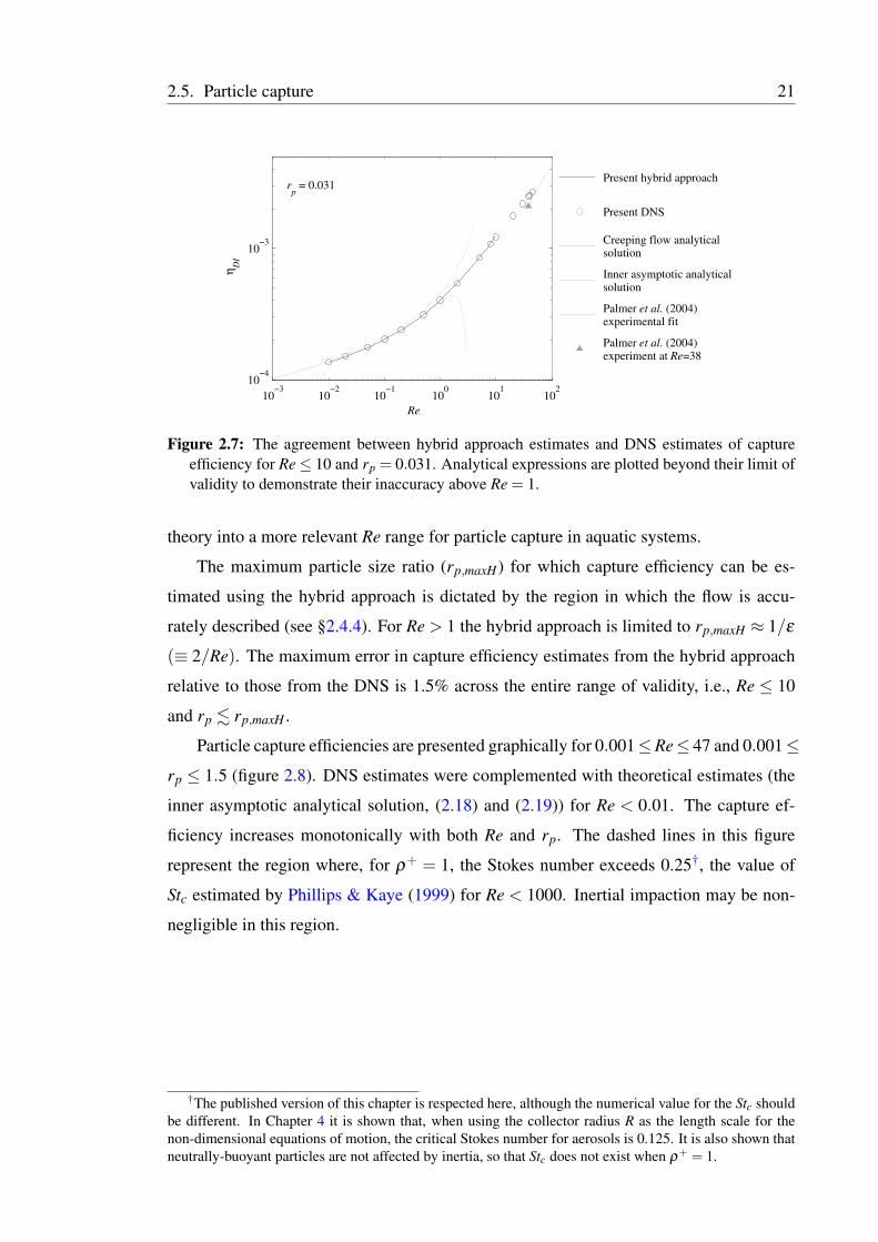
Figure 2.7: The agreement between hybrid approach estimates and DNS estimates of captureefficiency for Re≤ 10 and rp = 0.031. Analytical expressions are plotted beyond their limit ofvalidity to demonstrate their inaccuracy above Re = 1.

theory into a more relevant Re range for particle capture in aquatic systems.

The maximum particle size ratio (rp,maxH) for which capture efficiency can be es-

timated using the hybrid approach is dictated by the region in which the flow is accu-

rately described (see §2.4.4). For Re > 1 the hybrid approach is limited to rp,maxH ≈ 1/ε

(≡ 2/Re). The maximum error in capture efficiency estimates from the hybrid approach

relative to those from the DNS is 1.5% across the entire range of validity, i.e., Re ≤ 10

and rp . rp,maxH .

Particle capture efficiencies are presented graphically for 0.001≤Re≤ 47 and 0.001≤rp ≤ 1.5 (figure 2.8). DNS estimates were complemented with theoretical estimates (the

inner asymptotic analytical solution, (2.18) and (2.19)) for Re < 0.01. The capture ef-

ficiency increases monotonically with both Re and rp. The dashed lines in this figure

represent the region where, for ρ+ = 1, the Stokes number exceeds 0.25†, the value of

Stc estimated by Phillips & Kaye (1999) for Re < 1000. Inertial impaction may be non-

negligible in this region.

†The published version of this chapter is respected here, although the numerical value for the Stc shouldbe different. In Chapter 4 it is shown that, when using the collector radius R as the length scale for thenon-dimensional equations of motion, the critical Stokes number for aerosols is 0.125. It is also shown thatneutrally-buoyant particles are not affected by inertia, so that Stc does not exist when ρ+ = 1.

22 Chapter 2

10−3

10−2

10−1

100

101

10−7

10−6

10−5

10−4

10−3

10−2

10−1

100

Re

ηD

I

rp

1E−3

2E−3

3E−3

4E−3

6E−3

8E−30.01

0.02

0.03

0.04

0.06

0.080.10

0.20

0.300.40

0.60

1.001.50

Figure 2.8: Capture efficiency by direct interception (ηDI ) of a circular cylinder. Re is theReynolds number based on the diameter of the collector and rp is the particle-collector ra-dius ratio. Each line corresponds to a particular value of rp (labelled on the right). Dashedlines represent the region where the Stokes number exceeds 0.25† (for a particle density ratioof ρ+ = 1), such that particle inertia may influence particle capture.

2.6. Conclusions 23

Expressions for particle capture efficiency in creeping flow have previously been ob-

tained by assuming a linear variation of tangential velocity with distance from the cylinder

surface (Fuchs 1964; Friedlander 2000). This assumption, together with (2.28), yields an

expression of the form

ηDI(rp,Re)≈ 12

− ∂uθ

∂ r

∣∣∣∣ r=1,θ=θc0,

rp

2, (2.29)

which is valid for particles of vanishing size ratio. We propose a similar formulation that

is valid for all particle size ratios in the range 0 < rp ≤ 1.5 and over the entire Reynolds

number range considered here (0 < Re≤ 47). This formulation is given by

ηDI(rp,Re)≈ 12.002− lnRe+ f (Re)︸ ︷︷ ︸

G(Re)

· rp2

(1+ rp)k(Re)︸ ︷︷ ︸

Y (rp;Re)

, (2.30)

where G is a fit of (1/2)(−∂uθ/∂ r) at (r = 1,θ = θc0) and Y is a fit of the particle size

dependence of the capture efficiency. As the form of (2.30) suggests, the fitting procedure

was actually applied to the auxiliary functions f and k, yielding

f (Re) = 0.953ln(6.25+Re)−1.62, (2.31a)

k(Re) = 0.872ln(19.1+Re)−1.92. (2.31b)

The expression in (2.30) (together with (2.31)) provides capture efficiency estimates within

3% of our DNS estimates (and theory) over the entire particle size ratio and Reynolds

number ranges. The reciprocal of G in (2.30) is often termed the ‘hydrodynamic factor’

(Lee & Gieseke 1980). Its creeping flow form is preserved here, except for the addition of

the auxiliary function f , which allows an accurate representation of the maximum gradi-

ent of tangential velocity at the cylinder surface over the entire range of Re. The function

Y resembles the particle size dependence proposed by Lee & Gieseke (1980) for creeping

flow but has been modified such that that the exponent in the denominator (k) varies with

Re. The approximation Y ≈ r2p gives an error of less than 5% when rp≤ 0.05 and Re≤ 10.

2.6 Conclusions

We have obtained accurate estimates of the rate of capture of suspended particles by

cylindrical collectors in the ranges 0 < Re ≤ 47 and 0 < rp ≤ 1.5. In doing so, this

24 Chapter 2

work fills an existing gap between theoretical and experimental results in particle capture

research. The accuracy of the results is confirmed by their agreement with both theoretical

estimates at low Re and experimental data at higher Re. The analytical and graphical tools

presented here will allow considerable improvement in the prediction of particle capture

rates by biological collectors in aquatic systems. Furthermore, our analysis allows us

to present, for the first time, a physically based expression for estimating particle capture

efficiency for a particle size range relevant to aquatic systems and at all Reynolds numbers

below the onset of vortex shedding.

A hybrid approach has allowed the extension up to Re = 10 of an inner asymptotic

expansion for describing flow around a cylinder (2.18); it has been confirmed that the

existing theory is limited to Re . 1. This approach can be used for describing the flow

close to the surface of the entire cylinder when Re ≤ 1 and along the frontal face alone

when 1 < Re ≤ 10, allowing estimation of the capture efficiency and maximum angle of

capture with high accuracy. Our hybrid approach is likely to have significant utility for

applications that require an analytical description of the flow close to the cylinder surface

for Re∼ O(1−10).

The maximum angle of capture (αc) over the frontal face of the cylinder coincides

with the angle at which the radial velocity changes from negative to positive at a distance

equal to the radius of the particle; αc is less than 90◦ for Re& 0.001, a fact that has often

been overlooked in analytical studies of particle capture at low Re.

25

CHAPTER 3Particle capture by a circular cylinder in the

vortex-shedding regime†

3.1 Abstract

Particle capture, whereby suspended particles contact and adhere to a solid surface (a

‘collector’), is an important mechanism for a range of environmental processes including

suspension feeding by corals and ‘filtering’ by aquatic vegetation. In this paper, we use

two- and three-dimensional direct numerical simulations to quantify the capture efficiency

(η) of low-inertia particles by a circular cylindrical collector at intermediate Reynolds

numbers in the vortex-shedding regime (i.e. for 47 < Re≤ 1000, where Re is the collector

Reynolds number). We demonstrate that vortex shedding induces oscillations near the

leading face of the collector which greatly affect the quantity and distribution of captured

particles. Unlike in steady, low-Re flow, particles directly upstream of the collector are

not the most likely to be captured. Our results demonstrate the dependence of the time-

averaged capture efficiency on Re and particle size, improving the predictive capability for

the capture of particles by aquatic collectors. The transition to theoretical high-Reynolds-

number behaviour (i.e. η ∼ Re1/2) is complex due to comparatively rapid changes in

wake conditions in this Reynolds number range.

3.2 Introduction

‘Particle capture’ is a process by which particles in suspension contact a solid structure

(‘collector’) and adhere to its surface. Many environmental processes in aquatic systems

are controlled by particle-capture mechanisms: suspension feeding (Wildish & Krist-

manson 1997), seagrass pollination (Ackerman 2006), larval settlement (Harvey et al.

1995) and ‘filtering’ by aquatic vegetation (Palmer et al. 2004), among others. Despite

its ecological importance, the phenomenon of particle capture, particularly in the vortex-

shedding regime, remains poorly understood.

In particle-capture research, collectors are usually simplified as cylindrical structures

(representing the capturing filaments of suspension feeders or vegetation stems) and par-

ticles as spheres. The capture efficiency (η) of a cylindrical collector can be defined as

†A. Espinosa-Gayosso, M. Ghisalberti, G. N. Ivey and N. L. Jones, Particle capture by a circular cylinderin the vortex-shedding regime, Journal of Fluid Mechanics, 733: 171-188, 2013, doi:10.1017/jfm.2013.407

26 Chapter 3

the ratio of the number of particles captured (Nc) to the number of particles whose centres

would have passed through the space occupied by the collector were it not present in the

flow (Na):

η =Nc

Na. (3.1)

Here we consider perfect particle-collector adhesion, such that all particles are assumed

to be captured when they contact the cylinder surface.

As discussed by Espinosa-Gayosso et al. (2012), direct interception (where particle

centres follow the fluid exactly and contact with the collector occurs due to the finite

particle size) has been recognized as an important capture mechanism in aquatic sys-

tems (figure 3.1 displays the steady flow conceptualisation of particle capture by direct

interception). When compared with direct interception, inertial and diffusive effects on

particle capture are typically neglected in the aquatic systems of interest, due to the low

Stokes numbers (St) and high Péclet numbers (Pe) of suspended particles, respectively

(Espinosa-Gayosso et al. 2012). These two parameters are defined as

St =ρpD2

pU∞

9µD(3.2)

and

Pe =U∞D

Γp, (3.3)

where Dp is the particle diameter, D is the collector diameter, ρp is the particle density,

U∞ is the uniform upstream fluid velocity, µ is the fluid viscosity and Γp is the particle

diffusivity. Capture efficiency by direct interception depends on two different parameters

(Espinosa-Gayosso et al. 2012):

ηDI = ηDI(rp,Re), (3.4)

where rp is the particle size ratio and Re is the Reynolds number of the collector. The

definition of these two parameters is

rp =Dp

D≡ Rp

R(3.5)

and

Re =ρU∞D

µ, (3.6)

where Rp is the particle radius, R is the collector radius, ρ is the fluid density and µ is the

3.2. Introduction 27

α c

θc

R

Rp

2hU∞

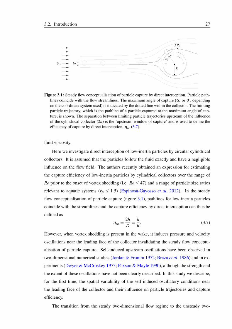
Figure 3.1: Steady flow conceptualisation of particle capture by direct interception. Particle path-lines coincide with the flow streamlines. The maximum angle of capture (αc or θc, dependingon the coordinate system used) is indicated by the dotted line within the collector. The limitingparticle trajectory, which is the pathline of a particle captured at the maximum angle of cap-ture, is shown. The separation between limiting particle trajectories upstream of the influenceof the cylindrical collector (2h) is the ‘upstream window of capture’ and is used to define theefficiency of capture by direct interception, ηDI (3.7).

fluid viscosity.

Here we investigate direct interception of low-inertia particles by circular cylindrical

collectors. It is assumed that the particles follow the fluid exactly and have a negligible

influence on the flow field. The authors recently obtained an expression for estimating

the capture efficiency of low-inertia particles by cylindrical collectors over the range of

Re prior to the onset of vortex shedding (i.e. Re ≤ 47) and a range of particle size ratios

relevant to aquatic systems (rp ≤ 1.5) (Espinosa-Gayosso et al. 2012). In the steady

flow conceptualisation of particle capture (figure 3.1), pathlines for low-inertia particles

coincide with the streamlines and the capture efficiency by direct interception can thus be

defined as

ηDI =2hD≡ h

R. (3.7)

However, when vortex shedding is present in the wake, it induces pressure and velocity

oscillations near the leading face of the collector invalidating the steady flow conceptu-

alisation of particle capture. Self-induced upstream oscillations have been observed in

two-dimensional numerical studies (Jordan & Fromm 1972; Braza et al. 1986) and in ex-

periments (Dwyer & McCroskey 1973; Paxson & Mayle 1990), although the strength and

the extent of these oscillations have not been clearly described. In this study we describe,

for the first time, the spatial variability of the self-induced oscillatory conditions near

the leading face of the collector and their influence on particle trajectories and capture

efficiency.

The transition from the steady two-dimensional flow regime to the unsteady two-

28 Chapter 3

dimensional vortex-shedding regime at Re1 ' 47 is not the only change in flow past a

circular cylinder that is relevant here. The next transition occurs at Re2 ' 180, when

three-dimensional vortex shedding appears; a second type of three-dimensional vortex

shedding starts at Re3 ' 260 (Williamson 1988; Henderson 1997). Another transition

occurs at Re4 ' 1000 due to the instability of the separating shear layers from the side

of the cylinder (Bloor 1964; Norberg 1994), with many others appearing at higher Re

(Williamson 1996; Zdravkovich 1997). Such transitions induce significant changes in

skin friction, wake pressure and the frequency of wake oscillation (Henderson 1995;

Williamson 1996), likely resulting in changes in capture efficiency.

Previous numerical (Haugen & Kragset 2010) and experimental (Palmer et al. 2004)

studies have suggested that, when Re > 47, the time-averaged capture efficiency of small

particles on circular cylinder collectors may be described by an expression of the form

ηDI ≈ k1Re0.7rp2, where k1 is a constant of proportionality. While simple, this expression

has three main disadvantages: (i) it fails to describe the changes induced by the flow

transitions mentioned above; (ii) it fails to describe the tendency towards the η ∼ Re1/2

proportionality predicted by boundary-layer theory for high-Re (Parnas & Friedlander

1984; Haugen & Kragset 2010); and (iii) it is restricted to particles of vanishing size

ratio (rp→ 0) (Friedlander 2000) while, in reality, aquatic collectors can capture particles

with rp ∼ O(1) (Harvey et al. 1995; Shimeta & Koehl 1997). Here we aim to provide a

physically-based description of capture efficiency that is free of such limitations.

In the present paper, we have used two- and three-dimensional direct numerical sim-

ulations (DNS) of flow past a circular cylinder to quantify particle capture by direct inter-

ception. Reynolds number and particle size ratio ranges relevant to aquatic systems are

considered (47 ≤ Re ≤ 1000 and 0 < rp ≤ 0.5). As part of this analysis, we investigate

the time-averaged and oscillatory components of the flow upstream of the collector and

the influence of these oscillations on particle trajectories and capture efficiency.

3.3 Basic equations of fluid motion and numerical methods

3.3.1 Equations of motion

The governing equations are the continuity and Navier-Stokes equations for unsteady and

incompressible flow. Here they are non-dimensionalized with the uniform free-stream

velocity U∞ as the velocity scale, and the radius of the collector R as the length scale:

3.3. Basic equations of fluid motion and numerical methods 29

∇ ·u = 0 (3.8)

and∂u∂ t

+(∇u)u =−∇p+2

Re∇

2u, (3.9)

where u is the non-dimensional velocity vector, p is the non-dimensional pressure, t is

the non-dimensional time and Re is the Reynolds number based on the diameter of the

collector, as defined by (3.6).

Most of our results are presented in a non-dimensional cylindrical coordinate system

(r,θ ,z) with the z-axis coincident with the axis of the collector and θ measured anticlock-

wise. We also make use of α , the angle measured from the leading edge in a clockwise

manner, as indicated in figure 3.1. When relevant, some quantities are presented in a non-

dimensional cartesian coordinate system (x,y,z) with the origin and the z-axis coincident

with the cylindrical system.

3.3.2 Spatial discretisation

For the two-dimensional DNS, the flow was solved in the rectangular domain −200 ≤x ≤ 80 and −200 ≤ y ≤ 200, which is wide enough to avoid blockage effects (Lange

et al. 1998; Posdziech & Grundmann 2007). The mesh topology is the same as in Wu

et al. (2004), where an H-type (rectangular) mesh is defined in most of the domain except

adjacent to the cylinder where an O-type ring (cylindrical mesh) is used, with a transition

region between the two mesh types. The O-type ring spanned from r = 1 (the collector

surface) to r = 1.2. The tangential direction of this ring was discretised into 744 uniform

cells and a non-uniform grid was used in the radial direction. The radial size of the cells

adjacent to the collector surface was ∆r≈ 1.0×10−3, less than the displacement thickness

at the leading edge for all Re considered here (Bouhairie & Chu 2007). The O-type mesh

merged smoothly into the H-type mesh, which started exactly at the square defined by the

diagonal points (−1.6,−1.6) and (1.6,1.6) in cartesian coordinates. The H-type mesh

covered the rest of the domain, with cell sizes gradually expanding from ∆x,y = 0.0065

to a maximum of ∆x,y = 1.6 close to the domain boundaries. A fine mesh size of at most

∆x,ywake = 0.05 was applied in the wake region.

For the three-dimensional DNS, the axial extent of the domain (−9.6≤ z≤ 9.6) was

greater than twice the size of the most unstable wavelength of mode-A three-dimensional

vortex shedding (Henderson 1997; Posdziech & Grundmann 2001). The axial direction

30 Chapter 3

was discretised into 128 uniform cells close to the cylinder, with a gradual reduction to 8

cells in the far field. A refinement of at least 32 cells was applied in the wake region.

3.3.3 Numerical methods and boundary conditions

The open-source code OpenFOAM R©† was used to solve (3.8) and (3.9) with a finite vol-

ume method of second order in space (Ferziger & Peric 2002) together with a three-level

backward scheme in time, which is also of second order (Ferziger & Peric 2002). The time

step was small enough to keep the maximum Courant number below 0.20. The pressure-

velocity coupling was solved with the PISO algorithm (Issa 1986) in which convergence

was deemed to be satisfied when the initial residuals of the pressure and momentum equa-

tions fell below 1×10−6.

The following velocity boundary conditions were applied: (i) no-slip no-flux bound-

ary conditions at the cylinder surface, (ii) a fixed uniform free-stream at the upstream

boundary ((ux,uy,uz) = (1,0,0) at xinlet = −200), (iii) a zero-gradient condition perpen-

dicular to the downstream boundary at xoutlet = 80, (iv) no-flux free-slip conditions at the

lateral boundaries (y=±200), and (v) cyclic conditions at the axial boundaries (z=±9.6)

in the three-dimensional DNS. For the pressure, a zero-gradient condition was applied at

all boundaries except the outlet, where a fixed value of poutlet = 0 was set, and at the

cyclic axial boundaries.

3.4 Flow conditions near the collector

3.4.1 The agreement between the present DNS and experimental

data

As discussed in §3.2, there are several regimes of flow past a circular cylinder for different

Re. Regime transitions induce changes in parameters such as the base suction coefficient

−Cpb =−Pb−P∞

12ρU2

∞

, (3.10)

the drag coefficient

CD =FD

12ρU2

∞D, (3.11)

†OpenFOAM R© is a registered trade mark of OpenCFD Limited, the producer of OpenFOAM software.

3.4. Flow conditions near the collector 31

101

102

103

0.2

0.4

0.6

0.8

1

1.2

Re

−C

pb

(a)

Re1 Re2 Re3 Re4

101

102

103

0

0.5

1

1.5

2

2.5

3

Re

CD

(b)

Re1 Re2 Re3 Re4

Figure 3.2: The agreement of the present DNS with existing experimental data for Re ≤ 1000.(a) Base suction coefficient −Cpb. (b) Drag coefficient CD. (N): Two-dimensional steady flowDNS (Espinosa-Gayosso et al. 2012). (•): Present two-dimensional DNS. (�): Present three-dimensional DNS. (×): Experiments of Williamson & Roshko (1990). (+): Experiments ofWieselsberger (1921). (The vertical lines indicate the regime transitions as explained in §§ 3.2and 3.4.1.)

and the Strouhal number

Str =D

U∞T; (3.12)

(see Henderson (1995; 1997)). Here, Pb is the time average of the pressure at the trailing

edge of the cylinder and P∞ is the pressure at the upstream boundary, FD is the time-

averaged drag force on the cylinder per unit length and T is the peak period of wake

oscillation.

The base suction coefficient varies significantly between regimes (figure 3.2a). At

low Re, the flow is steady and symmetric and the base suction decreases gradually with

increasing Re . Above Re1 ' 47, the flow becomes unstable and two-dimensional vortex

shedding appears in the wake; the time-averaged pressure at the trailing edge drops and

−Cpb increases with Re. At Re2 ' 180 and at Re3 ' 260 two more changes can be ob-

served as the flow transitions into distinct regimes of three-dimensional vortex shedding

(Williamson & Roshko 1990; Henderson 1997). As seen in figure 3.2(a), our DNS es-

timates of the base suction coefficient are in good agreement with existing experimental

data for Re≤ 1000. Our numerical estimates of the drag coefficient CD (figure 3.2b) and

the Strouhal number Str (not shown) are also in excellent agreement with experiment.

The relationships between these parameters and Re change dramatically at the transition

points (Henderson 1997). In §3.5.3, we show that capture efficiency exhibits similar be-

haviour.

32 Chapter 3

3.4.2 Oscillatory conditions near the leading face of the collector

A series of instantaneous tangential velocity profiles for Re = 180 reveal the presence

of oscillations along the leading face of the cylinder (figure 3.3). The profiles are shown

from the leading edge (α = 0) to α = 125◦, which is beyond the time-averaged separation

angle, αs. (Note that to preserve the idea of the mean flow moving clockwise along the

‘positive’ face of the cylinder (y > 0), the velocity component uα =−uθ is plotted instead

of the natural uθ .) These oscillations, which have a frequency equal to the wake oscillation

frequency, are more evident close to the leading edge, where the flow may reverse in

direction. In this figure, the small circles signify the location of the instantaneous velocity

maximum, a quantity which exhibits considerable variation close to the leading edge and

near the separation angle.

Although there are many theoretical and numerical studies of flow past a circular

cylinder with oscillatory boundary conditions (Glauert 1956; Watson 1959; Hori 1962;

Childs & Mayle 1984), they do not pertain here, as the strength and extent of the self-

induced oscillations vary spatially. A map of the local amplitude of the oscillations of the

tangential velocity for Re = 180 demonstrates this spatial variability (figure 3.4). Here,

the amplitude of oscillation is defined as the maximum of the difference between the

instantaneous and the time-averaged non-dimensional velocity component:

Auθ (r,θ) = max(|uθ (r,θ , t)−uθ (r,θ)|) . (3.13)

It is clear that Auθ varies with θ and r. Close to the leading face, Auθ exhibits a local max-

imum at the edge of the boundary layer; this maximal value increases from approximately

0.05 at α = 0 to 0.15 at αs (see also figure 3.3). Although upstream oscillation amplitudes

are small compared with those in the wake, they are far from negligible in the context of

particle capture; as will be shown in §3.5.4, the upstream oscillations deflect approaching

particles around alternating sides of the collector. Finally, the amplitude of oscillation

of the tangential velocity depends strongly on Re, this dependence varying with the flow

regime (figure 3.5).

3.4. Flow conditions near the collector 33

−0.05 0 0.050

0.2

0.4

0.6

0.8

r

α = 0◦

0 0.05

α = 1◦

0 0.05 0.1

α = 2◦

uα

0 0.05 0.1

α = 3◦

0 0.05 0.1 0.15 0.2

α = 5◦

0 0.50

0.2

0.4

0.6

0.8

r

α = 20◦

0 0.5 1

α = αc0 = 49.8◦

0 0.5 1 1.5

α = 90◦

uα

0 0.5 1

α = αs = 112.2◦

0 0.5 1

α = 125◦

Figure 3.3: Instantaneous (light grey) profiles of tangential velocity in the α direction (uα =−uθ )along the collector perimeter for Re = 180. Here r is the radial coordinate measured from thecylinder surface. The black lines represent the time-averaged profiles, with the black circlesshowing the edge of the boundary layer (taken as the point of zero velocity gradient). Thesmall circles indicate the point of zero gradient closest to the collector in each instantaneousvelocity profile. Note the different scale of the horizontal axis (uα ) for the profiles close to theleading edge (α ≤ 5◦). αc0 is the time average of the maximum angle of capture of particles ofvanishing size (rp→ 0) and αs is the time-averaged separation angle.

34 Chapter 3

Figure 3.4: The spatial variation of the non-dimensional amplitude of oscillation of the tangen-tial velocity component Auθ (logarithmic colour scale) for Re = 180. Close to the leadingface, Auθ exhibits a local maximum at the edge of the boundary layer which increases fromapproximately Auθ ≈ 0.05 at α = 0 to Auθ ≈ 0.15 at the separation angle.

102

103

0

0.01

0.02

0.03

0.04

0.05

0.06

0.07

Re

Auθ

Re1 Re2 Re3 Re4

Figure 3.5: The maximum amplitude of oscillation of the tangential velocity at α = 0 as a functionof Re. (•): Two-dimensional DNS. (�): Three-dimensional DNS. (The vertical lines indicatethe regime transitions as explained in §§ 3.2 and 3.4.1.)

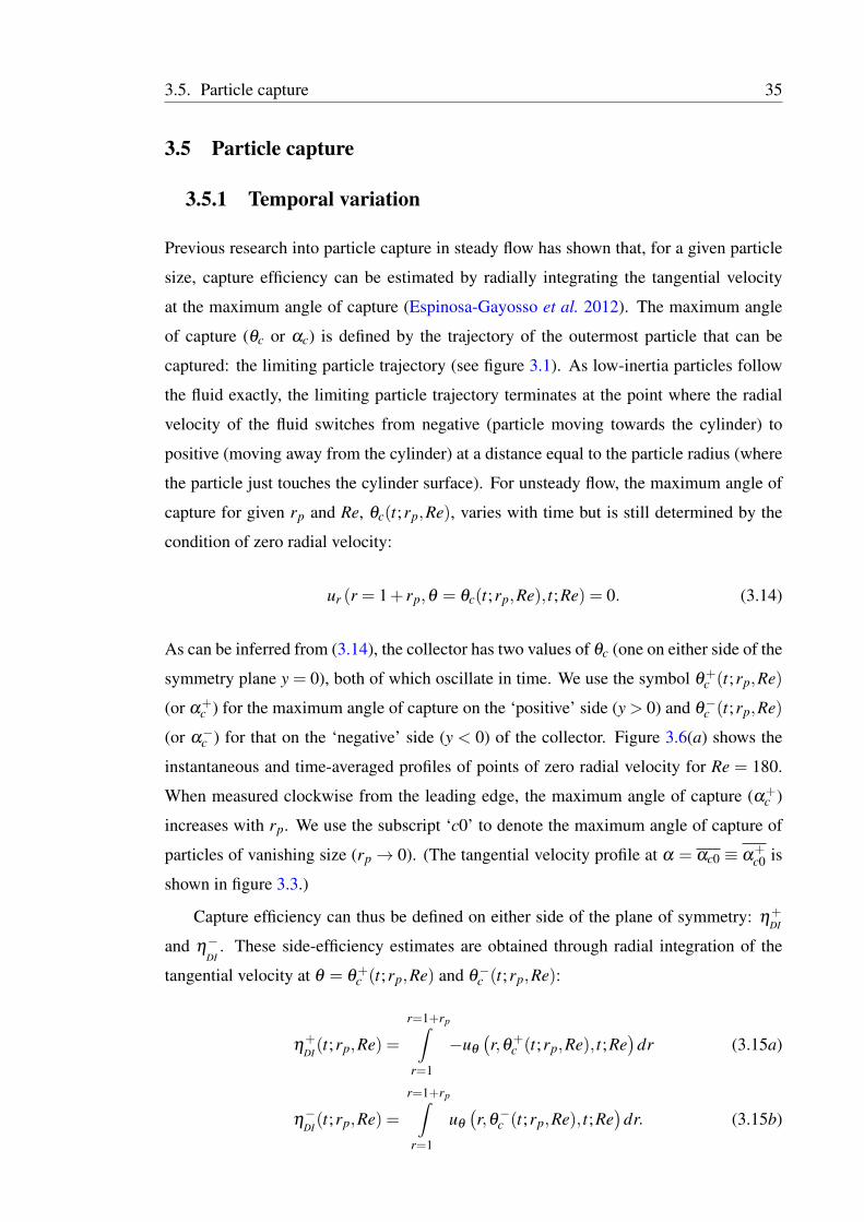
3.5. Particle capture 35

3.5 Particle capture

3.5.1 Temporal variation

Previous research into particle capture in steady flow has shown that, for a given particle

size, capture efficiency can be estimated by radially integrating the tangential velocity

at the maximum angle of capture (Espinosa-Gayosso et al. 2012). The maximum angle

of capture (θc or αc) is defined by the trajectory of the outermost particle that can be

captured: the limiting particle trajectory (see figure 3.1). As low-inertia particles follow

the fluid exactly, the limiting particle trajectory terminates at the point where the radial

velocity of the fluid switches from negative (particle moving towards the cylinder) to

positive (moving away from the cylinder) at a distance equal to the particle radius (where

the particle just touches the cylinder surface). For unsteady flow, the maximum angle of

capture for given rp and Re, θc(t;rp,Re), varies with time but is still determined by the

condition of zero radial velocity:

ur (r = 1+ rp,θ = θc(t;rp,Re), t;Re) = 0. (3.14)

As can be inferred from (3.14), the collector has two values of θc (one on either side of the

symmetry plane y = 0), both of which oscillate in time. We use the symbol θ+c (t;rp,Re)

(or α+c ) for the maximum angle of capture on the ‘positive’ side (y > 0) and θ−c (t;rp,Re)

(or α−c ) for that on the ‘negative’ side (y < 0) of the collector. Figure 3.6(a) shows the

instantaneous and time-averaged profiles of points of zero radial velocity for Re = 180.

When measured clockwise from the leading edge, the maximum angle of capture (α+c )

increases with rp. We use the subscript ‘c0’ to denote the maximum angle of capture of

particles of vanishing size (rp→ 0). (The tangential velocity profile at α = αc0 ≡ α+c0 is

shown in figure 3.3.)

Capture efficiency can thus be defined on either side of the plane of symmetry: η+DI

and η−DI

. These side-efficiency estimates are obtained through radial integration of the

tangential velocity at θ = θ+c (t;rp,Re) and θ−c (t;rp,Re):

η+DI(t;rp,Re) =

r=1+rp∫

r=1

−uθ

(r,θ+

c (t;rp,Re), t;Re)

dr (3.15a)

η−DI(t;rp,Re) =

r=1+rp∫

r=1

uθ

(r,θ−c (t;rp,Re), t;Re

)dr. (3.15b)

36 Chapter 3

−1 −0.5 0

0

0.5

1

1.5

2

y

x

α+c0

α+

rp

(a)

0 0.2 0.4 0.6 0.8 10.015

0.0155

0.016

0.0165

0.017

(t− t0) / T∗

η

(b)

η−DI

η+DI

ηDI

Figure 3.6: Temporal variation of variables related to particle capture for Re = 180. (a) Instan-taneous (light grey) and time-averaged (black) curves of points of zero radial velocity on the‘positive’ side of the collector. The time-averaged maximum angle of capture (α+) for a par-ticle of given size ratio (rp) is greater than the time-averaged maximum angle of capture (α+

c0)for particles of vanishing size (rp→ 0). (b) Temporal fluctuation of side (η±

DI) and overall (ηDI )

capture efficiencies for rp = 0.01 during one wake oscillation (of period T ∗), starting at anarbitrary instant t0.

The overall capture efficiency is the average of the two side-efficiencies:

ηDI(t;rp,Re) =12

η+DI(t;rp,Re)+

12

η−DI(t;rp,Re). (3.16)

The temporal behaviour of the side and overall capture efficiencies for Re = 180 and

rp = 0.01 is shown in figure 3.6(b), where T ∗ = TU∞/R is the non-dimensional period

of oscillation of the wake. While the unsteady velocity field generates oscillations in the

side efficiencies, these oscillations are out of phase such that the overall capture efficiency

remains effectively constant.

3.5.2 Time-averaged capture efficiency

As the time-averaged flow is symmetric with respect to the y = 0 plane, the time-averaged

capture efficiencies are identical:

ηDI = η+DI= η−

DI. (3.17)

Furthermore, the difference between ηDI and the capture efficiency estimated from the

time-averaged velocity field (ηDI ) was found to be negligible for all Re and rp analysed

3.5. Particle capture 37

0 50 100 150 200 250 300 350 400 450 5000

1

2

3

4

5

6x 10

−3

Re

ηDI

rp = 0.008

rp = 0.015

rp = 0.031

Figure 3.7: The agreement of DNS estimates (•) of time-averaged capture efficiency by directinterception (ηDI ) with experimental data from Palmer et al. (2004)(2), where the error barsrepresent the standard error. Dots are placed at the Reynolds numbers at which DNS wereperformed and the solid lines represent interpolated capture efficiency curves for each particlesize ratio (rp). Results for Re < 47 were obtained from Espinosa-Gayosso et al. (2012).

here. That is,

ηDI(rp,Re)≈ ηDI(rp,Re) =

r=1+rp∫

r=1

−uθ (r,θc(rp,Re);Re)dr, (3.18)

where

θc = θ+c =−θ

−c (3.19)

is defined by the time-averaged curve of zero radial velocity (figure 3.6a).

We have applied (3.18) to the numerically generated two- and three-dimensional flow

fields to estimate time-averaged capture efficiencies due to direct interception in the range

47 < Re ≤ 1000. This methodology assumes that forces on the particles such as lift

induced by shear, van der Waals attraction and hydrodynamic repulsion to contact may be

neglected to leading order, and we test this by comparing our particle-capture estimates

against existing experimental data. Our estimates are in excellent agreement with the

experiments of Palmer et al. (2004) and lie within their experimental range of error (figure

3.7). Note that results for Re < 47 are taken from Espinosa-Gayosso et al. (2012).

38 Chapter 3

0 0.025 0.050

0.01

0.02

rp

η DI

(a) Re = 50

0 0.025 0.050

0.01

0.02

rp

η DI

(b) Re = 180

0 0.025 0.050

0.01

0.02

rp

η DI

(c) Re = 1000

Figure 3.8: The quadratic dependence of capture efficiency on rp applies only to small particlesize ratios, as shown by the comparison of approximation (3.20) (−−) with estimates fromDNS (—). (a): Re = 50, (b): Re = 180, and (c): Re = 1000.

3.5.3 The dependence of capture efficiency on Re and rp

As discussed in §3.2, existing analytical expressions for particle capture do not fully

demonstrate the dependence of capture efficiency on Re and rp. The quadratic depen-

dence on rp is obtained through the approximation of a linear time-averaged profile of

tangential velocity (uθ (r)) in (3.18). That is,

ηDI(rp,Re)≈r=1+rp∫

r=1

|gc0(Re)|(r−1)dr =12|gc0(Re)|rp

2, (3.20)

where

gc0(Re)≡ ∂uθ (r,θc0;Re)∂ r

∣∣∣∣r=1

(3.21)

is the time-averaged gradient of tangential velocity at the collector surface evaluated at the

maximum angle of capture for particles of vanishing size. However, this approximation

of a linear velocity profile (3.20) is only valid in the limit of very low particle size, as

can be seen in the velocity profile at α = αc0 (figure 3.3). This is further demonstrated in

figure 3.8, where estimates of particle capture efficiency using (3.20) are compared with

those obtained from DNS.

3.5. Particle capture 39

The dependence of capture efficiency on Re will first be analysed for particles of

vanishing size. It is important to note that the capture efficiency of small particles is di-

rectly proportional to the surface velocity gradient gc0 (Weber & Paddock 1983; Espinosa-

Gayosso et al. 2012), as can be inferred from (3.20). (Also, gc0 is the maximum value of

the surface velocity gradient, and θc0 can therefore be interpreted as the angle of maxi-

mum local skin friction or maximum vorticity at the cylinder surface.) Figure 3.9 shows

the complex behaviour of the scaled velocity gradient |gc0|/Re1/2 with Re. Immediately

after the onset of vortex shedding (at Re1), |gc0| increases significantly, together with an

increase in the base suction (see also figure 3.2a). Close to this point, the dependence

|gc0| ∼ Re0.7 suggested by existing studies (as explained in §3.2 and indicated here by a

dashed curve) seems to apply but is valid only for 47 < Re. 100, and its usage for higher

Re may induce large errors. Across the full range of two-dimensional vortex shedding

(Re1 < Re < Re2), the maximum velocity gradient is better described by |gc0| ∼ Re0.65.

The behaviour of the scaled gradient changes as the flow transits into the regimes of

three-dimensional vortex shedding. In the range (Re3 < Re. 1000), the theoretical high-

Re dependence |gc0| ∼ Re1/2 (Schlichting 1979) is practically established, although this

dependence is expected to change again after the flow transition at Re4 ' 1000.

The error associated with estimation of capture efficiency of small particles from two-

dimensional DNS beyond Re = Re2 ' 180 can also be observed in figure 3.9. Relative

to three-dimensional DNS, hypothetical two-dimensional estimates (shown as unfilled

circles) overestimate the velocity gradient (and, therefore, the capture efficiency); this

overestimate reaches 13% at Re= 1000. Estimates from the hypothetical two-dimensional

DNS also fail to approach the theoretical high-Re dependence, ηDI ∼ Re1/2. This failure

is not due to the direct effect of oscillations on particle trajectories, as hypothesized by

Haugen & Kragset (2010), but arises when performing two-dimensional simulations of a

highly three-dimensional flow.

40 Chapter 3

101

102

103

0.8

0.9

1

1.1

1.2

1.3

Re

|gc0|/Re1/2

Re1 Re2 Re3 Re4

Figure 3.9: The dependence on Re of the time-averaged maximum velocity gradient at the collec-tor surface ( |gc0| , to which the capture efficiency of small particles is directly proportional).DNS results (two-dimensional steady flow DNS (Espinosa-Gayosso et al. 2012) (N), presenttwo-dimensional DNS (Re ≤ Re2 ' 180) (•) and present three-dimensional DNS (�)) showthe changes in behaviour across the different flow regimes. Hypothetical results from two-dimensional DNS above Re = Re2 are also shown (◦). The dashed line (−−) represents a|gc0| ∼ Re0.7 relationship. (The vertical lines indicate the regime transitions, as explained in§3.2 and §3.4.1.)

To summarize the results, the dependence of the capture efficiency on Re and rp is

presented in figure 3.10 for the range 1 ≤ Re ≤ 1000 and 0.001 ≤ rp ≤ 0.5 (results for

Re < 47 are taken from Espinosa-Gayosso et al. (2012)). For small particles, the capture

efficiency by direct interception behaves as explained in the preceding paragraphs of this

section. For large particles, the capture efficiency becomes independent of Reynolds num-

ber at large Re; more precisely, this occurs once the particle size significantly exceeds the

boundary layer thickness. The dotted lines represent the region where, for neutrally buoy-

ant particles, the Stokes number exceeds 0.25†, the critical value (for Re ≤ 1000) above

which particle inertia becomes important (Phillips & Kaye 1999). Inertial impaction may

not be negligible in this region. This diagram can be used for direct estimates of particle

capture efficiency for given Re and rp. (For the corresponding diagram at lower Re, see

Espinosa-Gayosso et al. (2012).)

†The published version of this chapter is respected here, although the numerical value for the criticalStokes number should be different. In Chapter 4 it is shown that, when using the collector radius R as thelength scale for the non-dimensional equations of motion, the critical Stokes number for aerosols is 0.125.It is also shown that neutrally-buoyant particles are not affected by inertia, so that the critical Stokes numberdoes not exist when ρ+ = 1.

3.5. Particle capture 41

100

101

102

103

10−6

10−5

10−4

10−3

10−2

10−1

100

Re

η DI

rp

0.001

0.002

0.003

0.005

0.010

0.020

0.030

0.050

0.100

0.200

0.500

Figure 3.10: Mean capture efficiency by direct interception (ηDI ) of a circular cylinder. Here Re isthe Reynolds number based on the diameter of the collector and rp is the particle-collector ra-dius ratio. Each line corresponds to a particular value of rp (labelled on the right). Dotted linesrepresent the region where the Stokes number exceeds 0.25† (for neutrally buoyant particles),such that particle inertia may influence particle capture.

42 Chapter 3

3.5.4 Effects of oscillations on particle trajectories

When vortex shedding is present, the self-induced oscillations upstream of the cylinder

(see §3.4.2) affect particle trajectories, modifying the simple steady flow conceptuali-

sation illustrated in figure 3.1. Particle trajectories, calculated from the DNS-generated

flow field, demonstrate this modification. Trajectories were obtained with a second-order

temporal scheme, using the same time step as in the DNS. A linear piecewise spatial

interpolation scheme (which generates a continuous velocity field at any position in the

domain) was used for estimating particle velocity, which was taken as that of the fluid at

the position of the particle centre.

The influence of upstream oscillations on particle trajectories is best illustrated by the

deformation of a line of particles released along the symmetry plane (figure 3.11). The

line of 10,000 particles (rp = 0.01) was released far upstream of the collector (in the range

−160 ≤ x ≤ −140) with equal spacing between particle centres. As we do not consider

interaction between particles, they were allowed to overlap in space to form an unbroken

line (shown in yellow). Importantly, in the case of steady upstream flow, all particles in

the line would be captured; that this does not happen here highlights the influence of flow

unsteadiness. As the particles approach the collector, the tip of the particle line is deflected

(figure 3.11a). (This first snapshot is for an arbitrary instant t = t0.) As time progresses,

the line of particles is then bent around the negative side of the collector, while a segment

following the tip continues to be stretched towards the positive side; this generates a ‘belt’

of particles around the leading face of the collector (figure 3.11b). When the flow close

to the leading edge reverses direction (figure 3.11c), the line is again stretched towards

the positive side. The stretching near the leading face is now more evident, as individual

particles (none of which have yet made contact with the collector) can be distinguished.

After the full cycle is completed (figure 3.11d), a second belt is formed. Only a small

fraction of particles from the first belt are captured (shown in black). This suggests that

in contrast to steady upstream flow (where particles in a narrow upstream window are

all captured), the upstream window of capture is much broader in the vortex-shedding

regime.

3.5. Particle capture 43

(a) t = t0 (b) t = t0 +1/3 T ∗

(c) t = t0 +2/3 T ∗ (d) t = t0 +T ∗

Figure 3.11: Oscillations, induced by vortex shedding, near the leading face of the collectorstretch and bend a line of particles (shown in yellow) towards alternating sides of the cylinder.The line of particles (rp = 0.01) was initially released upstream of the cylinder at the symmetryplane (y = 0). The panels show snapshots at: (a) t = t0, where t0 is an arbitrary instant; (b) t =t0 +1/3 T ∗; (c) t = t0 +2/3 T ∗; and (d) t = t0 +T ∗, where T ∗ is the period of wake oscillation.Whereas in the case of steady upstream flow, all released particles would be captured, onlya small fraction of particles (shown in black) are captured here, highlighting the importanceof upstream oscillations in the particle-capture process. The background color indicates theinstantaneous pressure coefficient Cp = 2(p− p∞). The Reynolds number is 180.

44 Chapter 3

−160 −155 −150 −145 −140−0.025

0

0.025

x

y

(a)

2h

2H

0 0.02 0.04 0.06 0.08−0.025

0

0.025

Πc

y

(b)

−50 −25 0 25 500

0.005

0.01

0.015

0.02

s c

α

(c)

Figure 3.12: Analysis of the spatial variation of particle capture for rp = 0.01 and Re = 180.(a) The upstream y-coordinates of particles that were captured on the leading face. The up-stream oscillations clearly modify the steady flow conceptualisation of particle capture: whilethe upstream positions still lie within a thin strip of width 2h, the strip has a near-sinusoidal de-formation of amplitude H. (b) The probability of capture (Πc) for a given particle as a functionof upstream position. Capture probability is greatest at the edges of the upstream window ofcapture and lowest at y = 0; at all positions, Πc� 1 (c) The probability density function sc(α)of the location of captured particles on the collector surface. sc has a maximum at the leadingedge of the collector (α = 0). For particles of vanishing size, the maximum angle of capture isconsistently ±50◦ in the vortex-shedding regime.

3.5. Particle capture 45

To identify the upstream window of capture (again for the case of Re = 180 and

rp = 0.01), a cloud of particles was released in the area (−160≤ x≤−140, −1≤ y≤ 1).

The initial position of particles captured on the leading face of the collector is shown

in figure 3.12(a) (the fraction of particles captured on the lee side of the collector was

less than 5%, and their initial positions are not shown). The initial lateral positions of

captured particles still lie within a thin strip whose width is related to capture efficiency

by (3.7), such that 2h = ηDI D remains applicable. However, due to the near-sinusoidal

shape of this strip, captured particles now come from a much wider upstream window of

capture (of width 2(H+h), where H is the amplitude of the strip’s sinusoidal shape). The

probability of capture for a given particle Πc(y) depends on its initial y coordinate (figure

3.12b). Particles initially at the symmetry plane are the least likely to be captured within

the upstream window of capture (Πc(y = 0) = 0.011), with maximal capture probability

at the edges of the window of capture. To summarise, in the case of steady upstream

flow, all particles released within ±h of the symmetry plane are captured. In the vortex-

shedding regime, a small fraction of particles released within the much wider ±(H + h)

range are captured, with capture probability varying with upstream position.

The probability density function (sc) of the location of captured particles on the col-

lector surface is shown in figure 3.12(c). Capture is most likely to occur at the leading

edge (α = 0), with the probability decaying to zero at the maximum angle of capture. For

the range of Re analysed (47 < Re ≤ 1000), the maximum angle of capture for particles

of vanishing size remained virtually constant αc0 ≈ 50◦. This is in good agreement with

the experiments of Palmer et al. (2004) and with our previous low-Re steady-state particle

capture analysis (Espinosa-Gayosso et al. 2012).

46 Chapter 3

3.6 Conclusions

We have used two- and three-dimensional DNS to obtain estimates of the capture ef-

ficiency of low-inertia particles by cylindrical collectors in ranges relevant to aquatic

systems: 47 < Re ≤ 1000 and 0 < rp ≤ 0.5. Our analysis allows us to present, for the

first time, a physically based description of capture efficiency by direct interception in

the vortex-shedding regime. The accuracy of the results is confirmed by their excellent

agreement with experiment.

The transition of flow around a circular cylinder set by changing Re induces shifts

in behaviour of commonly employed flow descriptors (namely the drag coefficient, the

base suction coefficient and the Strouhal number). Such changes are also observed in

the capture efficiency. In the range 260 . Re . 1000, where vortex shedding is three-

dimensional, the capture efficiency of small particles is well-approximated by ηDI ∼Re1/2, the dependence predicted by high-Re boundary-layer theory. For particle sizes

with radius significantly exceeding the boundary-layer thickness, capture efficiency by

direct interception becomes independent of the Reynolds number as it increases.

Vortex shedding induces oscillations upstream of the cylinder which considerably

influence the trajectories of low-inertia particles. These oscillations cause the particle

capture process in the vortex-shedding regime to be significantly different from the case

of steady upstream flow. Most notably, in the vortex-shedding regime, (i) the upstream

window of capture is much wider, (ii) the probability of capture for particles in the win-

dow is� 1, and (iii) particles along the symmetry plane (y = 0) are not the most likely to

be captured.

47

CHAPTER 4

Inertial effects on particle capture by circular collectors

in aquatic systems

4.1 Abstract

Particle capture, whereby suspended particles contact and adhere to a solid surface (a

‘collector’), is an important mechanism for a range of environmental processes includ-

ing suspension feeding by corals and ‘filtering’ by aquatic vegetation. Although particle

inertia is often ignored in the analysis of particle capture in aquatic systems, inertial ef-

fects can become important under certain conditions. It is generally believed that inertia

augments the capture efficiency when the Stokes number (St) of the particles exceeds a

critical value. In this paper, we use a numerical analysis of Lagrangian trajectories of

aquatic-type particles (where the ratio of particle density to fluid density is close to one)

to quantify the influence of inertia on particle capture in a parameter space relevant to

aquatic systems. First, we estimate the critical Stokes number for aquatic-type particles

and demonstrate its dependence on both the ratio of particle and fluid densities (ρ+) and

the Reynolds number (Re). Second, we analyse the capture of aquatic-type particles by

circular collectors. Our analysis shows that inertia can not only augment capture effi-

ciency but also diminish it, and that inertial effects appear well before the critical Stokes

number is reached. The role of particle inertia is maximised at Stokes numbers above the

critical value and can result in as much as a six-fold increase in the capture of particles

with a density similar to that of suspended sediment.

4.2 Introduction

‘Particle capture’ is a process by which particles in suspension contact a solid structure

(‘collector’) and adhere to its surface. This process is of great ecological importance

as it controls the feeding and the reproduction of many aquatic organisms (Shimeta &

Jumars 1991; Harvey et al. 1995; Wildish & Kristmanson 1997; Ackerman 2006), as well

as the ‘filtering’ of suspended particles by aquatic vegetation (Palmer et al. 2004). The

effects of particle inertia can become important under certain conditions but, despite their

relevance to ecological function, these effects have not yet been analysed in a parameter

space relevant to aquatic environments.

48 Chapter 4

α θx

yz

R

Rp

U∞

Figure 4.1: Steady flow conceptualisation of particle capture considering inertia and finite size.Particles are considered to be captured if they contact the collector. As the trajectories ofparticles influenced by inertia (indicated in black) do not coincide with the flow streamlines(indicated in grey), the capture efficiency of particles influenced by inertia (ηIN ) differs fromthe direct interception value (ηDI ). The limiting streamlines, which define ηDI for particlesof the same size (Espinosa-Gayosso et al. 2012; 2013), are indicated with dotted lines. TheCartesian coordinate system (x,y,z) and the direction of the angular measures α and θ , usedfor presenting our results, are also indicated.

Three different mechanisms of particle capture can occur on vertically-oriented col-

lectors (Friedlander 2000): (i) diffusional deposition, where particle-collector contact is

driven by random motions (such as Brownian motion), (ii) direct interception, where par-

ticle centres follow the fluid exactly and contact is made due to the finite particle size, and

(iii) inertial impaction where, due to particle inertia, trajectories no longer coincide with

fluid pathlines, thus affecting contact with the collector (figure 4.1). We have recently ob-

tained an accurate description of particle capture by direct interception covering a range

of particle sizes and flow conditions relevant to aquatic systems (Espinosa-Gayosso et al.

2012; 2013), and in the present study we extend this work by considering the effects of

particle inertia.

The process of particle capture is typically described for simplified geometries. Col-

lectors (such as vegetation stems or the capturing filaments of suspension feeders) are

modelled as cylinders, and particles (such as phytoplankton or suspended sediment) are

modelled as spheres. Furthermore, we consider perfect particle-collector adhesion, and

all particles are assumed to be captured when they contact the cylinder surface. For a

cylindrical collector, the capture efficiency (η) can be defined as the ratio of the number

of particles captured (Nc) to the number of particles whose centres would have passed

through the space occupied by the collector were it not present in the flow (Na):

η =Nc

Na. (4.1)

When diffusive effects are negligible, the capture efficiency for particles with inertia

4.2. Introduction 49

and finite size (ηIN ) depends upon three parameters:

ηIN = ηIN (rp,ρ+,Re), (4.2)

where rp is the particle size ratio, ρ+ is the particle density ratio and Re is the Reynolds

number of the collector. The definition of each of these parameters is as follows:

rp =Dp

D≡ Rp

R, (4.3)

ρ+ =

ρp

ρ, (4.4)

Re =ρU∞D

µ, (4.5)

where Dp and Rp are the particle diameter and radius, D and R are the collector diameter

and radius, ρp is the particle density, ρ is the fluid density, U∞ is the uniform upstream

fluid velocity and µ is the fluid viscosity. Particles influenced by inertia do not follow

fluid pathlines exactly (streamlines in steady flow), as shown in figure 4.1. The capture

efficiency for particles with inertia (ηIN ) thus differs from the direct interception value

(ηDI ) for the same particle size ratio and Re. In the limit of high particle inertia, particles

are not influenced by the flow field and travel in straight-line trajectories in the streamwise

direction. In this limit, the capture efficiency is therefore given by

ηIN,max = 1+ rp. (4.6)

Note that the definition of capture efficiency (4.1) allows efficiencies to be greater than 1,

as can be seen in (4.6) (see also Espinosa-Gayosso et al. (2012; 2013)); this occurs when

particles with centres outside the window defined by the collector diameter are captured.

The parameter typically chosen to represent the importance of particle inertia is the

Stokes number (St) (Friedlander 2000), as this non-dimensional group appears naturally

in the drag term of the particle momentum equation for aerosols (ρ+� 1). The definition

of St incorporates rp, ρ+ and Re:

St =ρpD2

pU∞

9µD=

ρ+r2pRe

9. (4.7)

Inertial impaction is typically thought to become dominant for aerosols once St exceeds

a critical value; however, inertial effects have been observed even when St is well below

50 Chapter 4

the critical value due to compressibility of the particle phase (Robinson 1956; Michael

1968; Fernandez de la Mora & Rosner 1982; Fernandez de la Mora 1986; Maxey 1987).

The existence of a critical Stokes number for aerosols (Stc,ae) was first demonstrated by

Taylor (1940), who analysed particles of negligible size (but with finite St) approaching an

object along the stagnation streamline. For inviscid flow and a cylindrical collector, it was

found that particles reached the collector in a finite time only if the Stokes number was

above Stc,ae,inv = 1/8. However, it has been recognized that the critical Stokes number

varies with the Reynolds number (Langmuir 1948; Davies & Peetz 1956; Matsufuji &

Hasegawa 1986; Lesnic et al. 1994; Phillips & Kaye 1999). Furthermore, accurate values

of the critical Stokes number for aerosol particles in viscous flow (Stc,ae,ν ) for Re≤ 1000

have not yet been determined. Here we examine the critical Stokes number for aerosols

in viscous flow with low-to-intermediate Re using Taylor’s ‘classical’ approach, before

focusing on particles with ρ+ ∼ O(1), which are typical of aquatic systems.

There has been considerable analytical and experimental research into the effects of

inertia on the capture of aerosols (see, e.g., Davies & Peetz (1956); Fuchs (1964); Fernan-

dez de la Mora & Rosner (1982); Fernandez de la Mora (1986); Wessel & Righi (1988);

Flagan & Seinfeld (1988); Friedlander (2000); Haugen & Kragset (2010)). However, such

studies are not applicable to aquatic systems as they are characterised by one or more of

the following conditions: (i) very high particle density ratios (ρ+� 1), (ii) a focus on a

narrow range of flow conditions (usually inviscid or creeping flow fields, which can be

described analytically), (iii) neglect of the finite particle size (rp� 1), and/or (iv) a focus

on a range of St where inertial impaction is entirely dominant. In aquatic systems, the

particles of interest have a density similar to that of water (ρ+ ∼ O(1)), the flow condi-

tions cover a wide range of Re (0 < Re . 1000), particle sizes can be of the order of the

collector diameter (rp ∼ O(1)), and St is in a range where both direct interception and

inertial impaction may be dominant. The effects of inertia on particle capture have yet to

be described in a parameter space relevant to aquatic systems.

Due to the low particle density ratio (ρ+∼O(1)), the equations of motion for aquatic-

type particles cannot be simplified to the equations commonly used for aerosols (Babiano

et al. 2000); the dynamics of aquatic-type particles are very different to those of aerosols

in a wide range of flow conditions (Maxey 1987; Babiano et al. 2000; Haller & Sapsis

2008). Furthermore, when particles are neutrally buoyant (ρ+ = 1), inertial effects are

almost completely suppressed; while the behaviour of such particles is very close to that

of a perfect tracer, it can differ in zones with large fluid velocity gradients (Babiano et al.

4.3. Basic equations of motion and numerical methods 51

2000). Here we analyse how the particle density ratio modifies the critical Stokes con-

cept and the capture efficiency for aquatic systems. We extend the classical procedure

of Taylor (1940) to aquatic-type particles in inviscid and viscous flow to determine the

dependence of the critical Stokes number on ρ+ and Re. We also use a numerical scheme

to evaluate the effects of inertia on the capture efficiency of aquatic-type particles by cal-

culating their Lagrangian trajectories in mean flow fields (with time and axial averages

obtained from direct numerical simulation (DNS)). We compare the capture efficiencies

of particles with inertia (ηIN ) to those when inertia is not considered (i.e. pure direct

interception, Espinosa-Gayosso et al. (2012; 2013)) and discuss the reasons behind the

differing behaviours.

4.3 Basic equations of motion and numerical methods

4.3.1 Equations of fluid motion

The governing equations are the continuity and Navier-Stokes equations for incompress-

ible flow. Here they are non-dimensionalized with the uniform free-stream velocity U∞ as

the velocity scale, and the radius of the collector R as the length scale:

∇ ·u = 0 (4.8)

and∂u∂ t

+(∇u)u =−∇p+2

Re∇

2u, (4.9)

where u is the non-dimensional fluid velocity vector, p is the non-dimensional pressure, t

is the non-dimensional time and Re is the Reynolds number based on the diameter of the

collector, as defined by (4.5).

Most results are presented in a non-dimensional cylindrical coordinate system (r,θ ,z)

with the z-axis coincident with the axis of the collector and θ measured anti-clockwise

(figure 4.1). When relevant, results are presented in a non-dimensional Cartesian coordi-

nate system (x,y,z) with the origin and the z-axis coincident with the cylindrical system.

4.3.2 Equations of particle motion

Here we consider the influence of the fluid flow on particle motion but neglect the in-

fluence of the particles on the fluid motion. Particle-particle interaction effects are also

neglected. The Lagrangian equations for each particle (Maxey & Riley 1983; Auton et al.

52 Chapter 4

1988; Babiano et al. 2000) can be written in non-dimensional form as:

dxc

dt= vc (4.10)

ρ+dvc

dt=

Duc

Dt− 9

r2pRe

(vc−uc)−12

(dvc

dt− Duc

Dt

)(4.11)

where xc is the non-dimensional position vector of the centre of the particle, vc is the non-

dimensional velocity of the particle (measured at its centre) and uc = u(x = xc(t), t) is the

fluid velocity at the position of the particle at any instant (consistent with the assumption

that particles do not disturb the fluid); (vc− uc) therefore represents the velocity of the

particle relative to the fluid. The terms on the right of (4.11) are the horizontal forces

acting on the particle and represent, respectively, the fluid acceleration, the Stokes drag

and the added mass effect. As in Babiano et al. (2000), we are neglecting additional forces

due to Faxén corrections and Basset-Boussinesq history. The derivative Duc/Dt is taken

along the path of a fluid element,

Duc

Dt=

∂uc

∂ t+(∇uc)uc, (4.12)

while the derivative duc/dt is taken along the trajectory of the particle,

duc

dt=

∂uc

∂ t+(∇uc)vc, (4.13)

so thatDuc

Dt=

duc

dt− (∇uc)(vc−uc). (4.14)

The particle momentum equation (4.11) can then be rewritten as

dvc

dt=−

(2ρ+

2ρ++1

)1St(vc−uc)+

32ρ++1

Duc

Dt. (4.15)

If dealing with aerosols (ρ+� 1), (4.15) can be further simplified to

dvc

dt=− 1

St(vc−uc). (4.16)

However, for aquatic systems with ρ+ ∼ O(1), all the terms in (4.15) must be retained.

Following Babiano et al. (2000), we substitute (4.14) into (4.15) and rewrite it in terms of

4.3. Basic equations of motion and numerical methods 53

the relative particle velocity to obtain

ddt

(vc−uc) =−(

2ρ+

2ρ++1

)1St(vc−uc)−

32ρ++1

(∇uc)(vc−uc)−2(ρ+−1)2ρ++1

duc

dt.

(4.17)

This form of the momentum equation shows that perfectly neutrally-buoyant particles

(ρ+ = 1), for which the last term on the right hand side of (4.17) disappears, behave as

perfect tracers only if the second term (the one containing the fluid velocity gradient)

can also be neglected. In that case, after some initial difference between the particle and

the fluid velocities, the relative particle velocity would decay exponentially with time

(Babiano et al. 2000) and particles would follow fluid paths exactly. But when the fluid

velocity gradient is large (as in zones close to stagnation points,Babiano et al. (2000)) or

when the particles are not perfectly neutrally-buoyant, the two last terms on the RHS of

(4.17) induce particle dynamics which differ from both those of a perfect tracer and those

characterised by the common aerosol simplification (4.16).

4.3.3 Numerical methods for estimating particle trajectories

Capture efficiencies and critical Stokes numbers were estimated with a Lagrangian ap-

proach by ‘seeding’ particles within a series of fully-developed flow solutions (obtained

from DNS as described in Espinosa-Gayosso et al. (2012; 2013) using the open-source

Navier-Stokes solver code OpenFOAM R©† v2.1.x). Both the fluid velocity and velocity

gradient fields were imported into MATLAB R©† release 2013b, and the particle trajecto-

ries calculated within the framework of this numerical tool. When Re ≤ 47, the flow is

steady; above this value of Re, the flow is unsteady. However, calculation of particle tra-

jectories in unsteady flow fields is very computationally expensive. Consequently, in this

range of higher Re, DNS flow fields were first axially- and time-averaged into mean flow

fields before particle trajectories were calculated. For Re > 180, at least 50 oscillation cy-

cles of fully-developed flow were used for the averaging in time, as the flow is no longer

perfectly time-periodic when three-dimensional vortex shedding is present (Henderson

1997).

For the particle capture estimates, ‘clouds’ of particles of finite size were seeded into

the computational domain upstream of the cylinder with an initial velocity equal to that

of the fluid at the particles’ initial positions (i.e. vc(t = 0) = uc). For critical Stokes num-

†OpenFOAM R© is a registered trade mark of OpenCFD Limited, the producer of OpenFOAM software.†MATLAB R© is a registered trade mark of The MathWorks Inc., Natick, Massachusetts, U.S.A.

54 Chapter 4

ber estimates, a single ‘point’ particle was seeded on the stagnation streamline for each

St tested, and the St was incremented by 0.0001 until a particle was able to reach the

stagnation point. In the seeding zone, the fluid velocity was always within 0.01% of the

uniform flow condition, i.e. (u,v,w) ≈ (U∞,0,0). Particle trajectories were obtained by

integrating (4.10) and (4.17) using an algorithm based on the explicit Runge-Kutta (4,5)

pair formula of Dormand & Prince (1980). The fluid velocity and the velocity gradient

at the particle centre (uc and ∇uc) were obtained with a linear piecewise spatial interpo-

lation of the mean DNS fields, which generates continuous fields at any position in the

domain. The time-step always satisfied ∆t < 0.1St, a requirement for accurate simulation

of particle motion (Dorgan & Loth 2007). Particles were deemed to be captured when

they touched the collector (i.e. when their centre came within one particle radius of the

collector surface). Capture efficiency was estimated using (4.1) after all the non-captured

particles had exited the domain.

4.4 The critical Stokes number

Taylor (1940) estimated the critical Stokes number for aerosol particles in inviscid flow

(Stc,ae,inv). This value defines the minimum neccessary St for ideal ‘point’ aerosol parti-

cles (that started with the same velocity as the fluid) to reach the stagnation point when

moving along the stagnation streamline of an inviscid flow past a cylinder. Here we extend

Taylor’s analysis of aerosols to viscous flow at Re ≤ 1000 and to aquatic-type particles

with ρ+ ∼ O(1).

4.4.1 The critical Stokes number for aerosols in inviscid flow

The non-dimensional velocity field of inviscid flow past a circular cylinder in cylindrical

coordinates is

(ur,uθ ) =

(cosθ

(1− 1

r2

),−sinθ

(1+

1r2

))(4.18)

(White 2008). Along the stagnation streamline (θ = π), the fluid moves in the negative

radial direction only, i.e.,

(ur,uθ )θ=π=

(−(

1− 1r2

),0). (4.19)

Zero velocity is reached at the stagnation point (i.e. at the leading edge of the cylinder,

(r,θ) = (1,π)). The trajectory of an ideal ‘point’ aerosol particle (rp = 0 but with finite

St) approaching the collector along this stagnation streamline is obtained by substituting

4.4. The critical Stokes number 55

(4.10) and (4.19) into the momentum equation for aerosol particles (4.16), which can then

be rewritten as

Std2rc

dt2 +drc

dt+

(1− 1

rc2

)= 0, (4.20)

where rc denotes the radial position of the point particle. As this equation has no analytical

solution, Taylor (1940) further simplified (4.20) by approximating its non-homogeneous

term as a linear function of distance from the stagnation point, resulting in the simplified

equation of motion

Std2rc

dt2 +drc

dt+2(rc−1) = 0. (4.21)

The general solution of (4.21) is

rc(t) =

e−t

2St

(A e

t√

1−8St2St +B e−

t√

1−8St2St

)+1 for St < 1/8

e−4t (A+ Bt)+1 for St = 1/8

e−t

2St

(A cos t

√8St−12St + B sin t

√8St−12St

)+1 for St > 1/8

(4.22)

(Phillips & Kaye 1999), where the A’s and B’s are integration constants that depend on

the initial position and initial velocity, which is considered equal to that of the fluid at the

initial position. The characteristic equation for the associated homogeneous equation of

(4.21) is

St m2 +m+2 = 0, (4.23)

and the changes in behaviour of the solution (4.22) depend on the values of the roots of

(4.23). The characteristic discriminant

∆ = 1−8St, (4.24)

determines the values of the characteristic roots. The value of St for which ∆ = 0 (i.e.

the critical Stokes number for aerosols in inviscid flow, Stc,ae,inv = 1/8) defines a transi-

tion in the behaviour of the solutions. Particles with St ≤ Stc,ae,inv have ∆ ≥ 0 (i.e. real

and negative characteristic roots) and never reach the stagnation point (r = 1) because

rc(t) > 1 at all times. Only those particles with St > Stc,ae,inv have ∆ < 0 (i.e. imaginary

characteristic roots) and reach the stagnation point (i.e. rc(t)≤ 1 at some finite time) due

to the oscillatory nature of the solution.

Numerical estimates of the critical Stokes number were obtained by solving the lin-

earised equation (4.21) and the exact equation (4.20) using the methodology explained

56 Chapter 4

in §4.3.3 adapted for the use of analytical fluid velocity fields. From the numerical so-

lution of linearised equation (4.21) we obtained a critical Stokes number for aerosols in

inviscid flow of Stnumc,ae,inv = 0.1251, in near-perfect agreement with linear inviscid the-

ory. The numerical solution for the exact momentum equation (4.20) (i.e. with the full

non-homogeneous term) shows that the exact critical Stokes number is slightly higher,

Stnum,exactc,ae,inv = 0.1260.

4.4.2 The critical Stokes number for aquatic-type particles in in-

viscid flow

When the added mass effect and the fluid forces terms are retained in the particle mo-

mentum equation (4.17), the critical Stokes number differs from that of aerosols. The

trajectory of a ‘point’ particle (rp = 0 but with finite St and ρ+ ∼ O(1)) approaching

the collector along the stagnation streamline is defined by substituting (4.10), (4.13) and

(4.19) into (4.17), which can then be rewritten as

(2ρ++1

2ρ+

)St

d2rc

dt2 +drc

dt+

(1− 3St

ρ+r3c

)(1− 1

rc2

)= 0. (4.25)

(note that this equation simplifies to (4.20) for ρ+� 1.) Following the approach by Taylor

(1940), we approximate the non-homogeneous term as a linear function of distance from

the stagnation point. The simplified equation of motion is

(2ρ++1

2ρ+

)St

d2rc

dt2 +drc

dt+2(

1− 3Stρ+

)(rc−1) = 0, (4.26)

with characteristic discriminant

∆ = 1−8St(

2ρ++12ρ+

)(1− 3St

ρ+

). (4.27)

Particles with St values for which ∆ becomes negative will reach the stagnation point. The

condition ∆ = 0 defines a quadratic equation for St,

12(2ρ

++1)

St2c,inv−4ρ

+(2ρ

++1)

Stc,inv +ρ+2

= 0, (4.28)

for which its smaller root determines the critical Stokes number. This critical value (Stc,inv)

varies with ρ+ and tends to the aerosol value, Stc,ae,inv, when ρ+� 1 (figure 4.2); the crit-

ical Stokes number exceeds the aerosol value for ρ+. 1.5 and tends to 1/6 when ρ+→ 1

4.4. The critical Stokes number 57

1 2 3 4 50.1

0.11

0.12

0.13

0.14

0.15

0.16

0.17

0.18

0.19

0.2

ρ+

St c

,inv

Figure 4.2: The critical Stokes number for aquatic-type particles in inviscid flow (Stc,inv) increasesas ρ+ → 1. However, Stc,inv does not exist for ρ+ ≤ 1 (as indicated by the circles). Thedashed-dotted line (-.-) is for Stc,inv, the critical Stokes number obtained from the analysisof the linearised theory (4.28). The continuous line (—) is for Stnum,exact

c,inv , the critical Stokesnumber obtained from the numerical solution of the exact momentum equation (4.25).

from the right. When ρ+ ≤ 1, the characteristic discriminant (4.27) is never negative and

the solution of (4.26) never changes form. Therefore, ideal point particles with a density

equal to or less than that of the surrounding fluid will never reach the stagnation point

(when starting with the same velocity as the fluid) and the critical Stokes number does

not exist for ρ+ ≤ 1. The numerical solution of the exact momentum equation (4.25)

shows that the exact values of the critical Stokes number are indeed slightly higher that

the values obtained from the linearised theory.

4.4.3 Critical Stokes number for aquatic-type particles in viscous

flow

When a viscous flow is considered, the critical Stokes (Stc,ν ) differs from the inviscid

value (Stc,inv) due to differences in the radial velocity profile close to the stagnation point.

Conservation of mass (4.8), together with the no-slip condition at the cylinder surface,

imply that the radial velocity and its gradient in the radial direction are both zero at the

collector surface i.e.

ur = 0 and∂ur

∂ r= 0 at r = 1. (4.29)

Viscous flow is thus more gradually-varying close to the collector than inviscid flow (fig-

ure 4.3), and the drag force acting on the particles moving along the stagnation streamline

is lower, requiring additional mass (higher St) in order to acquire enough momentum to

58 Chapter 4

11.021.041.061.081.1−0.1

−0.08

−0.06

−0.04

−0.02

0

r

ur| θ=

π

Re = 1000

Re = 100

Re = 10

Re →∞

Figure 4.3: The mean radial velocity profile along the stagnation streamline (ur|θ=π) varies more

gradually as the influence of viscosity increases. The lines represent inviscid flow (Re→ ∞,from (4.19)) and DNS results at Re = 10,100 and 1000. The horizontal axis has been reversedto maintain the mental picture of the stagnation point (r = 1) on the right with r increasing tothe left.

reach the collector (Davies & Peetz 1956; Phillips & Kaye 1999). By considering two re-

gions in the flow field, (i) a viscous boundary-layer region close to the stagnation point and

(ii) an inviscid flow region in the far field, Phillips & Kaye (1999) were able to estimate

the critical Stokes number for aerosol particles in viscous flow (Stc,ae,ν ) for Re ≥ 1000.

Here, we estimate Stc,ν values in a range relevant to aquatic ecosystems (i.e. Re ≤ 1000

and ρ+ ∼ O(1)), using the numerical methodology explained in §4.3.3.

Equation (4.17) was solved along the mean stagnation streamlines obtained from

DNS for a range of Reynolds numbers and particle density ratios. For the mean flow

conditions, (4.13) is used to simplify the last term in (4.17). For aerosols (ρ+ � 1),

the critical Stokes number increases as Re decreases and, at low Re, exceeds the invis-

cid value by up to two orders of magnitude (figure 4.4). Even at Re = 1000 the value

of Stc,ν for aerosols is more than double that of Stc,ae,inv (in agreement with Phillips &

Kaye (1999)). For aquatic-type particles with a density ratio similar to that of suspended

sediment (ρ+ = 2.6) there is only a small increase of the critical Stokes number when

compared to aerosols, except when Re is less than 0.3, for which the increase is signifi-

cant. Finally, for near-neutrally-buoyant particles (ρ+ = 1.1) the critical Stokes number

is clearly greater than the aerosol value (by more than 50% for all Re). Neutrally-buoyant

particles and those with smaller density than the surrounding fluid did not reach the stag-

nation point for any St.

Although the critical Stokes number is typically thought to indicate the point at which

4.5. Inertial effects on the efficiency of capture of aquatic-type particles 59

10−2

10−1

100

101

102

103

104

105

106

10−1

100

101

Re

St c,ν

Stc,ae,inv

ρ+= 1.1

ρ+= 2.6

ρ+≫ 1

P & K

Figure 4.4: The critical Stokes number in viscous flow (Stc,ν ) increases with decreasing Re andas ρ+→ 1. For aquatic-type particles, values of Stc,ν (obtained by DNS) for two particle den-sity ratios are shown: that for sediment-type particles (ρ+ = 2.6), and that for near-neutrally-buoyant particles (ρ+ = 1.1). The critical Stokes number for aerosols (Stc,ae,ν ) is labeled asρ+ � 1. There is no curve for neutrally-buoyant particles because Stc,ν does not exist inthat case. The results of the analytical approximation of Phillips & Kaye (1999) for aerosolsis labeled as (P & K). The theoretical value for aerosols in inviscid flow (i.e. as Re→ ∞),Stc,ae,inv = 1/8, is also indicated.

inertia starts to affect the capture of very small particles (Phillips & Kaye 1999), in the

next section we determine the Stokes number at which the capture of aquatic-type parti-

cles of finite size is actually affected by inertia.

4.5 Inertial effects on the efficiency of capture of aquatic-type parti-

cles

Here, we describe the effect of inertia on the capture efficiency of aquatic-type particles

(ρ+ ∼ O(1)) over ranges of Re and St (or rp) common to aquatic systems. The results

using the procedure described in §4.3.3 are presented and compared to the capture effi-

ciencies estimated by considering only direct interception (Espinosa-Gayosso et al. 2012;

2013).

We found neutrally-buoyant particles (ρ+= 1) follow almost perfectly the trajectories

defined by the mean streamlines. The difference of particle capture efficiency compared

to that of pure direct interception is less than 0.1% for Re ≤ 1000 and rp ≤ 1.5. For the

Re tested here, the strength of the velocity gradients is not sufficient to cause particles to

deviate from effectively perfect tracer behaviour and only direct interception should thus

be considered in this case (Espinosa-Gayosso et al. 2012; 2013).

60 Chapter 4

For the case of sediment-type particles (ρ+ = 2.6), as expected, inertia increases cap-

ture efficiency with increasing St (figure 4.5); the vertical lines labelled as P in this figure

show the points at which the capture efficiency increases by 10% relative to direct inter-

ception. Note that this 10% increase occurs before reaching the critical Stokes number for

viscous flow Stc,ν . At the critical Stokes value, the increase in capture efficiency reaches

50% for Re = 10 and 100% for Re = 1000; the maximum increase induced by inertia is

as large as 500% for Re = 1000 (figure 4.5d). Aquatic-type particle dynamics differ from

those of aerosols, such that the increase of ηIN with St does not approach the limit of very

high particle inertia (ηIN,max).

Inertia can diminish capture efficiency under certain conditions (Fernandez de la

Mora 1986). In our tests for ρ+ = 2.6 and Re & 100, inertia initially reduces the cap-

ture efficiency relative to direct interception before an increase occurs at higher St; the

vertical line labelled as N in figure 4.5(d) shows the St at which the capture efficiency de-

creases by 10% compared to direct interception. For Re = 1000, the reduction occurs in

the range 0.001. St . 0.17, and is as large as 40%. This reduction in capture efficiency

occurs as particles drift away from the collector due to centrifugal acceleration (Fernandez

de la Mora 1986). The effect is illustrated in figure 4.6(a), which displays the trajectory

of a particle with weak inertial influence (St = 0.11 and rp = 0.02) which is released on

the outer-most streamline that allows capture of neutrally buoyant particles of this size

(the limiting streamline for direct interception defined by Espinosa-Gayosso et al. (2012;

2013)). A neutrally-buoyant particle would follow the limiting streamline exactly and

reach the collector at the maximum angle of capture of zero-inertia particles of that size

(αc,DI), but a particle influenced by inertia deviates from that trajectory. At first, close to

the leading edge of the collector, the particle with weak inertial influence separates from

the curving limiting streamline, and its trajectory gets closer to the collector. But, at its

point of minimum distance from the collector, the particle has not been captured yet (fig-

ure 4.6b) and the centrifugal drift induced by the particle inertia subsequently allows it to

escape. This weak inertial influence results in fewer particles reaching the collector, and a

lower capture efficiency compared to neutrally-buoyant particles (i.e. due purely to direct

interception). The reduction in capture efficiency appears well before any critical Stokes

number estimated in §4.4.

4.5. Inertial effects on the efficiency of capture of aquatic-type particles 61

10−3

10−2

10−1

100

101

102

103

10−4

10−3

10−2

10−1

100

101

102

St

η

Stc,ν

(a)

Re = 1

ηIN

ηDI

ηIN,max

10−1

100

101

rp

10−3

10−2

10−1

100

101

102

103

10−4

10−3

10−2

10−1

100

101

102

St

P Stc,ν

(b)

Re = 10

ηIN

ηDI

ηIN,max

10−1

100

101

rp

10−3

10−2

10−1

100

101

102

103

10−4

10−3

10−2

10−1

100

101

102

St

η

P Stc,ν

(c)

Re = 100

ηIN

ηDI

ηIN,max

10−2

10−1

100

rp

10−3

10−2

10−1

100

101

102

103

10−4

10−3

10−2

10−1

100

101

102

St

PN Stc,ν

(d)

Re = 1000

ηIN

ηDI

ηIN,max

10−2

10−1

100

rp

Figure 4.5: Capture efficiencies for sediment-type particles (ρ+ = 2.6) as a function of St for (a)Re = 1; (b) Re = 10; (c) Re = 100; and (d) Re = 1000. The capture efficiency (ηIN ) consideringinertia and finite particle size is compared to that for direct interception (ηDI ) and to that in theextreme limit of maximum inertial impaction (ηIN,max) (4.6). The Stokes numbers at which anincrease of 10% compared to ηDI exists are indicated with a P (positive difference) and thosewith a decrease of 10% are indicated with an N (negative difference). The secondary horizontalaxis indicates the corresponding particle size ratio, rp, for the sediment-type particles.

62 Chapter 4

α c,DI

(a)

10 20 30 40 50 60 70 80 90

0.015

0.02

0.025

0.03

0.035

0.04

0.045

0.05

α

r

(b)

α c,DI

Figure 4.6: Graphical analysis of the centrifugal drift that induces a reduction in capture efficiencyfor sediment-type particles with weak inertial influence (ρ+ = 2.6, St = 0.11, rp = 0.02, Re =1000).(a): Plot of the trajectory of a particle with weak inertia influence (shown in black) that isreleased on the limiting streamline for direct interception of particles of that size (shown as adotted line). The particle with weak inertial influence (shown in black) separates from the lim-iting streamline, but does not reach the collector and drifts centrifugally, therefore decreasingthe capture efficiency with respect to direct interception. The capture position of a neutrally-buoyant particle of the same size (shown in grey) and the maximum angle of capture for directinterception (αc,DI) are also indicated.(b): Distance from the collector surface (r = r− 1) with respect to the angle measured fromthe leading edge of the collector (α). At first, the distance from the collector to the trajectoryof the centre of a particle with weak inertia influence (continuous black line) diminishes withα , but the minimum distance is still larger than its radius (indicated with a horizontal dashedline) and capture never occurs. The distance from the collector to the corresponding limitingstreamline (dotted line) meets the capture criteria at αc,DI .

4.6. Conclusions 63

4.6 Conclusions

For aquatic-type particles, we have used a Lagrangian analysis to estimate the influence

of inertia on particle capture. We have shown that the velocity gradients for Re ≤ 1000

are not strong enough to induce significant deviations of neutrally-buoyant particles from

a perfect-tracer trajectory, such that the only mechanism of capture for neutrally buoy-

ant particles is direct interception. When the particle density ratio is similar to that of

sediment in water, the effects of inertia are two-fold: (i) inertia augments the capture ef-

ficiency when the Stokes number is sufficiently large, and (ii) counter-intuitively, inertia

can reduce capture for particles with weak inertial influence, i.e., lower St.

For the first time, the critical Stokes number for aerosols in viscous flow conditions

(Stc,ae,ν ) has been described for 0.01≤ Re≤ 1000; in this range, Stc,ae,ν increases consid-

erably with decreasing Re. We also present, for the first time, an analysis of the critical

Stokes number for non-aerosol particles (aquatic-type particles) in viscous (Stc,ν ) and in-

viscid flow (Stc,inv). Compared to the aerosol value, the critical Stokes number increases

as the particle density approaches that of the surrounding fluid. Finally, when ρ+ ≤ 1,

the critical Stokes number does not exist and ‘point’ particles never reach the stagnation

point. However, when analysing the capture of aquatic-type particles of finite size with

a density ratio similar to that of suspended sediment (ρ+ = 2.6), we have shown that

inertial effects appear at values of St much lower than the critical value. At the critical

Stokes number, the increase in capture efficiency exceeds 50% for Re > 10. The impact

of particle inertia on capture is maximised when St > Stc,ν and can result in as much as a

six-fold increase in capture efficiency.

64 Chapter 4

65

CHAPTER 5Conclusions

This research has served to advance knowledge in two basic fields of science. First, it

has improved our understanding of the fundamental fluid mechanics problem of flow past

a circular cylinder. Secondly, it has vastly improved the available tools for estimating

particle capture in aquatic systems.

With respect to the new understanding of flow past a circular cylinder, I extend exist-

ing analytical descriptions of the flow field close to the leading face of the cylinder up to

Re = 10. This is likely to have significant utility for analytical studies of diffusional de-

position and heat and mass transfer. With the aid of accurate two- and three-dimensional

direct numerical simulations, the spatial variation of the upstream oscillations induced by

the oscillatory wake and the dependence of their amplitude on Re are shown for the first

time. I also present novel insight into the magnitude and exact angle of the maximum

shear stress or vorticity (which coincides with the maximum angle of capture of small

particles) at the cylinder surface for Re≤ 1000.

With respect to the particle capture process, I provide the necessary tools for accu-

rately estimating particle capture by direct interception for relevant particle size ratios in

the range Re≤ 1000, filling a knowledge gap in particle capture research. The capture ef-

ficiency of small particles is found to be directly related to the maximum velocity gradient

at the collector surface, which occurs at the maximum angle of capture. This result is used

to develop an expression for capture efficiency by direct interception for rp ≤ 1.5 in the

steady flow regime. For the vortex shedding regime and when considering inertia, only

graphical tools for predicting capture efficiency are presented, as formulations covering

the range of flow conditions and particle sizes are too complicated to employ.

The present work can facilitate significant improvement in the understanding of ecosys-

tem function in aquatic environments by allowing researchers to accurately estimate cap-

ture efficiencies without the restrictions on Re and rp of existing expressions. As dis-

cussed in the introduction and by several other authors (Shimeta & Jumars 1991; Wildish

& Kristmanson 1997; Palmer et al. 2004; Humphries 2009), flow conditions and par-

ticle size ratios for aquatic ecosystems applications may easily be above the analytical

restrictions of Re = 1 or rp� 1. The range of Re and rp covered here is suitable for esti-

mates of particle capture in aquatic ecosystems to applications such as particle retention

in wetlands and tidal marshes, larvae capture, seagrass pollination and suspension feed-

66 Chapter 5

ing. Diagrams in figures 2.8 and 3.10 and equation (2.30) provide accurate estimates of

capture efficiency when the flow conditions (Re) and particle size to collector size ratio

(rp) are used as independent parameters.

Detailed analysis of the flow conditions in the capture process show that, when vortex

shedding is present, oscillations in the wake of the collector induce upstream oscillations

in the vicinity of the collector’s leading face. These oscillations affect particle trajecto-

ries considerably, modify the upstream window of capture, and enhance the capture of

particles approaching the cylinder away from the plane of symmetry. Despite the oscil-

latory flow conditions around the collector, oscillations in total capture were found to be

negligible, and capture efficiencies can be obtained from time-averaged flow fields. This

greatly simplifies the numerical process for estimating capture efficiency when consider-

ing particle inertia.

Direct interception estimates can also be used as the baseline in quantification of the

effects of other influences, such as particle inertia. It was found that inertia does not

affect neutrally-buoyant particle trajectories when Re ≤ 1000, so that direct interception

diagrams and expressions should be used when ρ+ = 1. However, for particles similar

to suspended sediment (ρ+ = 2.6), inertia can both augment and diminish capture effi-

ciency. The reduction in capture efficiency occurs at higher Reynolds numbers due to the

centrifugal drift of particles with weak inertial influence. The zones of influence of inertia

for sediment-type particles as a function of Re and St are identified.

This work represents an essential first step towards a complete understanding of par-

ticle capture in aquatic systems, but further research is necessary. As the numerical tools

used here have successfully simulated the effects of inertia on the capture of aquatic-type

particles, the next step is to complete capture efficiency formulations and diagrams cov-

ering the range of density ratios of aquatic particles. More complicated extensions are

driven by the fact that many aquatic systems are wave-influenced, necessitating the study

of particle capture in oscillatory flow. The influence of free-stream turbulence is also of

principal interest. Research on the influence of turbulence on related processes such as

heat and mass transfer remains an important topic for the turbulence research community.

Methodologies from the studies of these related processes can be incorporated into the

research of particle capture in both aerosol and aquatic systems. Finally, the analysis of

particle capture by collector arrays (of varying configurations) will prove to be highly

valuable and especially relevant to aquatic ecosystems.

67

Bibliography

ACKERMAN, J. D. 1997a Submarine pollination in the marine angiosperm Zostera ma-

rina (zosteraceae) .I. the influence of floral morphology on fluid flow. Am. J. Bot. 84 (8),

1099–1109.

ACKERMAN, J. D. 1997b Submarine pollination in the marine angiosperm Zostera ma-

rina (zosteraceae). II. pollen transport in flow fields and capture by stigmas. Am. J. Bot.

84 (8), 1110–1119.

ACKERMAN, J. D. 2006 Sexual reproduction of seagrasses: Pollination in the marine

context. In Seagrasses: Biology, ecology and conservation (ed. A.W.D. Larkum, R.J.

Orth & C.M. Duarte). Amsterdam: Springer.

AUTON, T. R., HUNT, J. C. R. & PRUDHOMME, M. 1988 The force exerted on a body

in inviscid unsteady non-uniform rotational flow. J. Fluid Mech. 197, 241–257.

BABIANO, A., CARTWRIGHT, J. H. E., PIRO, O. & PROVENZALE, A. 2000 Dynamics

of a small neutrally buoyant sphere in a fluid and targeting in Hamiltonian systems.

Phys. Rev. Lett. 84 (25), 5764–5767.

BLOOR, M. S. 1964 The transition to turbulence in the wake of a circular cylinder. J.

Fluid Mech. 19 (2), 290–304.

BOUHAIRIE, S. & CHU, V. H. 2007 Two-dimensional simulation of unsteady heat trans-

fer from a circular cylinder in crossflow. J. Fluid Mech. 570, 177–215.

BRAZA, M., CHASSAING, P. & MINH, H. H. 1986 Numerical study and physical anal-

ysis of the pressure and velocity fields in the near wake of a circular cylinder. J. Fluid

Mech. 165, 79–130.

CHILDS, E. P. & MAYLE, R. E. 1984 Heat transfer on a rotationally oscillating cylinder

in cross-flow. Int. J. Heat Mass Transf. 27 (1), 85–94.

68

CRESSWELL, J. E., DAVIES, T. W., PATRICK, M. A., RUSSELL, F., PENNEL, C.,

VICOT, M. & LAHOUBI, M. 2004 Aerodynamics of wind pollination in a zoophilous

flower, Brassica napus. Funct. Ecol. 18 (6), 861–866.

DAVIES, C. N. 1950 Viscous flow transverse to a circular cylinder. Proc. Phys. Soc. Lon.

Sec.-B 63 (364), 288–296.

DAVIES, C. N. & PEETZ, C. V. 1956 Impingement of particles on a transverse cylinder.

Proc R Soc Lon Ser-A 234 (1197), 268–295.

DORGAN, A. J. & LOTH, E. 2007 Efficient calculation of the history force at finite

Reynolds numbers. Int. J. Multiphas. Flow 33 (8), 833–848.

DORMAND, J. R. & PRINCE, P. J. 1980 A family of embedded Runge-Kutta formulae.

J. Comput. Appl. Math. 6 (1), 19–26.

DWYER, H. A. & MCCROSKEY, W. J. 1973 Oscillating flow over a cylinder at large

Reynolds-number. J. Fluid Mech. 61 (4), 753–767.

ESPINOSA-GAYOSSO, A., GHISALBERTI, M., IVEY, G. N. & JONES, N. L. 2012 Par-

ticle capture and low-Reynolds-number flow around a circular cylinder. J. Fluid Mech.

710, 362–378.

ESPINOSA-GAYOSSO, A., GHISALBERTI, M., IVEY, G. N. & JONES, N. L. 2013 Par-

ticle capture by a circular cylinder in the vortex-shedding regime. J. Fluid Mech. 733,

171–188.

FERNANDEZ DE LA MORA, J. 1986 Inertia and interception in the deposition of particles

from boundary-layers. Aerosol Sci. Technol. 5 (2), 261–286.

FERNANDEZ DE LA MORA, J. & ROSNER, D. E. 1982 Effects of inertia on the diffu-

sional deposition of small particles to spheres and cylinders at low Reynolds numbers.

J. Fluid Mech. 125, 379–395.

FERZIGER, J.H. & PERIC, M. 2002 Computational Methods for Fluid Dynamics, 3rd

edn. Springer.

FLAGAN, R. C. & SEINFELD, J. H. 1988 Fundamentals of air pollution engineering, 1st

edn.

69

FRIEDLANDER, S. K. 1967 Particle diffusion in low-speed flows. J. Colloid Interface

Sci. 23 (2), 157–164.

FRIEDLANDER, S. K. 2000 Smoke, Dust and Haze. Fundamentals of Aerosol Dynamics,

2nd edn. Oxford University Press.

FUCHS, N. A. 1964 The mechanics of aerosols, 1st edn. Pergamon Press.

GLAUERT, M. B. 1956 The laminar boundary layer on oscillating plates and cylinders. J.

Fluid Mech. 1 (1), 97–110.

HALLER, G. & SAPSIS, T. 2008 Where do inertial particles go in fluid flows? Physica D

237 (5), 573–583.

HARVEY, M., BOURGET, E. & INGRAM, R. G. 1995 Experimental evidence of passive

accumulation of marine bivalve larvae on filamentous epibenthic structures. Limnol.

Oceanogr. 40 (1), 94–104.

HAUGEN, N. E. L. & KRAGSET, S. 2010 Particle impaction on a cylinder in a crossflow

as function of Stokes and Reynolds numbers. J. Fluid Mech. 661, 239–261.

HENDERSON, R. D. 1995 Details of the drag curve near the onset of vortex shedding.

Phys. Fluids 7 (9), 2102–2104.

HENDERSON, R. D. 1997 Nonlinear dynamics and pattern formation in turbulent wake

transition. J. Fluid Mech. 352, 65–112.

HORI, E.-I. 1962 Unsteady boundary layers, 3rd report, boundary layer on a circular

cylinder in rotational oscillation. Bull. JSME 5 (17), 64–72.

HUMPHRIES, S. 2009 Filter feeders and plankton increase particle encounter rates

through flow regime control. Proc. Natl. Acad. Sci. U. S. A. 106 (19), 7882–7887.

HUNER, B. & HUSSEY, R. G. 1977 Cylinder drag at low Reynolds number. Phys. Fluids

20 (8), 1211–1218.

ISSA, R. I. 1986 Solution of the implicitly discretized fluid-flow equations by operator-

splitting. J. Comput. Phys. 62 (1), 40–65.

JORDAN, S. K. & FROMM, J. E. 1972 Oscillatory drag, lift, and torque on a circular

cylinder in a uniform flow. Phys. Fluids 15 (3), 371–376.

70

KAPLUN, S. 1957 Low Reynolds number flow past a circular cylinder. J. Math. Mech

6 (4), 595–603.

KELLER, J. B. & WARD, M. J. 1996 Asymptotics beyond all orders for a low Reynolds

number flow. J. Eng. Math. 30 (1-2), 253–265.

LAMB, H. 1911 On the uniform motion of a sphere through a viscous fluid. Philos. Mag.

Series 6, V. 21 (121), 112–121.

LANGE, C. F., DURST, F. & BREUER, M. 1998 Momentum and heat transfer from

cylinders in laminar crossflow at 10−4 ≤ Re ≤ 200. Int. J. Heat Mass Transf. 41 (22),

3409–3430.

LANGMUIR, I. 1948 The production of rain by a chain reaction in cumulus clouds at

temperatures above freezing. J. Meteorol. 5 (5), 175–192.

LEE, B. E., FLETCHER, C. A. J., SHIN, S. H. & KWON, S. B. 2002 Computational

study of fouling deposit due to surface-coated particles in coal-fired power utility boil-

ers. Fuel 81 (15), 2001–2008.

LEE, K. W. & GIESEKE, J. A. 1980 Note on the approximation of interceptional collec-

tion efficiencies. J. Aerosol. Sci. 11 (4), 335–341.

LESNIC, D., ELLIOTT, L. & INGHAM, D. B. 1994 Characterizations of the critical

Stokes number for potential and viscous flows. Mathematika 41 (82), 277–292.

MATSUFUJI, H. & HASEGAWA, E. 1986 Critical condition for collision of suspended

small particles with a body in a viscous-fluid. Bull. JSME 29 (256), 3375–3382.

MAXEY, M. R. 1987 The motion of small spherical particles in a cellular flow field. Phys.

Fluids 30 (7), 1915–1928.

MAXEY, M. R. & RILEY, J. J. 1983 Equation of motion for a small rigid sphere in a

nonuniform flow. Phys. Fluids 26 (4), 883–889.

MICHAEL, D. H. 1968 The steady motion of a sphere in a dusty gas. J. Fluid Mech.

31 (1), 175–192.

NORBERG, C. 1994 An experimental investigation of the flow around a circular cylinder:

influence of aspect ratio. J. Fluid Mech. 258, 287–316.

71

OPENFOAM 2012 The open source cfd toolbox. http://www.openfoam.com/.

OSEEN, C. W. 1910 Über die Stokes’sche Formel, und über eine verwandte Aufgabe in

der Hydrodynamik. Ark. Mat. Astr. Fys. 6 (29), 1–20.

PALMER, M. R., NEPF, H. M., PETTERSSON, T. J. R. & ACKERMAN, J. D. 2004

Observations of particle capture on a cylindrical collector: Implications for particle

accumulation and removal in aquatic systems. Limnol. Oceanogr. 49 (1), 76–85.

PARNAS, R. & FRIEDLANDER, S. K. 1984 Particle deposition by diffusion and intercep-

tion from boundary-layer flows. Aerosol Sci. Technol. 3 (1), 3–8.

PATANKAR, S. V. 1980 Numerical heat transfer and fluid flow, 1st edn. Taylor and Fran-

cis.

PAXSON, D. E. & MAYLE, R. E. 1990 Velocity measurements on the forward portion of

a cylinder. J. Fluids Eng.-Trans. ASME 112 (2), 243–245.

PHILLIPS, C. G. & KAYE, S. R. 1999 The influence of the viscous boundary layer on the

critical Stokes number for particle impaction near a stagnation point. J. Aerosol. Sci.

30 (6), 709–718.

POSDZIECH, O. & GRUNDMANN, R. 2001 Numerical simulation of the flow around an

infinitely long circular cylinder in the transition regime. Theor. Comput. Fluid Dyn.

15 (2), 121–141.

POSDZIECH, O. & GRUNDMANN, R. 2007 A systematic approach to the numerical cal-

culation of fundamental quantities of the two-dimensional flow over a circular cylinder.

J. Fluids Struct. 23 (3), 479–499.

PROUDMAN, I. & PEARSON, J. R. A. 1957 Expansions at small Reynolds numbers for

the flow past a sphere and a circular cylinder. J. Fluid Mech. 2 (3), 237–262.

ROBINSON, A. 1956 On the motion of small particles in a potential field of flow. Comm.

Pure Appl. Math. 9 (1), 69–84.

RUBENSTEIN, D. I. & KOEHL, M. A. R. 1977 Mechanisms of filter feeding: Some

theoretical considerations. Am. Nat. 111 (981), 981–994.

SCHLICHTING, H. 1979 Boundary-layer theory, 7th edn. McGraw-Hill.

72

SEBENS, K. P. & KOEHL, M. A. R. 1984 Predation on zooplankton by the benthic

anthozoans Alcyonium siderium (Alcyonacea) and Metridium senile (Actiniaria) in the

New England subtidal. Mar. Biol. 81 (3), 255–271.

SEN, S., MITTAL, S. & BISWAS, G. 2009 Steady separated flow past a circular cylinder

at low Reynolds numbers. J. Fluid Mech. 620, 89–119.

SHIMETA, J. 1993 Diffusional encounter of submicrometer particles and small-cells by

suspension feeders. Limnol. Oceanogr. 38 (2), 456–465.

SHIMETA, J. & JUMARS, P. A. 1991 Physical mechanisms and rates of particle capture

by suspension-feeders. Oceanogr. Mar. Biol. 29, 191–257.

SHIMETA, J. & KOEHL, M. A. R. 1997 Mechanisms of particle selection by tentaculate

suspension feeders during encounter, retention, and handling. J. Exp. Mar. Biol. Ecol.

209 (1-2), 47–73.

SKINNER, L. A. 1975 Generalized expansions for slow flow past a cylinder. Q. J. Mech.

Appl. Math. 28 (3), 333–340.

STOKES, G. G. 1851 On the effect of the internal friction of fluids on the motion of

pendulums. Trans. Cambridge Philos. Soc 9 (Part II), 8–106.

STUMPF, R. P. 1983 The process of sedimentation on the surface of a salt marsh. Estuar.

Coast. Shelf Sci. 17 (5), 495–508.

TAYLOR, G.I. 1940 Note on possible equipment and technique for experiments on icing

on aircraft. Reports and Memoranda of the Aeronautical Research Committee (No.

2024).

TRITTON, D. J. 1959 Experiments on the flow past a circular cylinder at low Reynolds

numbers. J. Fluid Mech. 6 (4), 547–567.

DE VASCONCELOS, T. F., SAPOVAL, B., ANDRADE, J. S., GROTBERG, J. B., HU,

Y. Y. & FILOCHE, M. 2011 Particle capture into the lung made simple? J. Appl.

Physiol. 110 (6), 1664–1673.

VEYSEY, J. & GOLDENFELD, N. 2007 Simple viscous flows: From boundary layers to

the renormalization group. Rev. Mod. Phys. 79 (3), 883–927.

73

WATSON, J. 1959 The two-dimensional liminar flow near the stagnation point of a cylin-

der which has an arbitrary transverse motion. Q. J. Mechanics Appl. Math. 12 (2),

175–190.

WEBER, M. E. & PADDOCK, D. 1983 Interceptional and gravitational collision efficien-

cies for single collectors at intermediate Reynolds-numbers. J. Colloid Interface Sci.

94 (2), 328–335.

WESSEL, R. A. & RIGHI, J. 1988 Generalized correlations for inertial impaction of

particles on a circular-cylinder. Aerosol Sci. Technol. 9 (1), 29–60.

WHITE, F. M. 2008 Fluid mechanics, 6th edn. McGraw-Hill.

WIESELSBERGER, C. 1921 Neuere feststellungen über die gesetze des flüssigkeits- und

luftwiderstands. Phys. Z. 22, 321–328.

WILDISH, D. & KRISTMANSON, D. 1997 Benthic suspension feeders and flow, 1st edn.

Cambridge University Press.

WILLIAMSON, C. H. K. 1988 The existence of two stages in the transition to three-

dimensionality of a cylinder wake. Phys. Fluids 31 (11), 3165–3168.

WILLIAMSON, C. H. K. 1996 Vortex dynamics in the cylinder wake. Ann. Rev. Fluid

Mech. 28, 477–539.

WILLIAMSON, C. H. K. & ROSHKO, A. 1990 Measurements of base pressure in the

wake of a cylinder at low Reynolds numbers. Z. Fluwiss. Weltraumforsch. 14 (1-2),

38–46.

WU, M. H., WEN, C. Y., YEN, R. H., WENG, M. C. & WANG, A. B. 2004 Experi-

mental and numerical study of the separation angle for flow around a circular cylinder

at low Reynolds number. J. Fluid Mech. 515, 233–260.

ZDRAVKOVICH, M. M. 1997 Flow around circular cylinders. Vol1: Fundamentals, ,

vol. 1. Oxford University Press.