participation in contract farming and its effects on
TRANSCRIPT

PARTICIPATION IN CONTRACT FARMING AND ITS EFFECTS ON TECHNICAL
EFFICIENCY AND INCOME OF VEGETABLE FARMERS IN WESTERN KENYA
ALULU JOSEPH
A56/9487/2017
A THESIS SUBMITTED IN PARTIAL FULFILMENT OF THE REQUIREMENTS FOR
THE AWARD OF THE DEGREE OF MASTER OF SCIENCE IN AGRICULTURAL
AND APPLIED ECONOMICS
DEPARTMENT OF AGRICULTURAL ECONOMICS
FACULTY OF AGRICULTURE
UNIVERSITY OF NAIROBI
2020

i
DECLARATION
This thesis is my original work and has not been submitted to any other University for any other
award.
Alulu Joseph
Reg. No. A56/9487/2017
Signature……………………………… Date………………………………………
This thesis has been submitted with our approval as university supervisors.
1. Dr. David Jakinda Otieno
Department of Agricultural Economics, University of Nairobi.
Signature Date: 03rd July 2020
2. Prof. Willis Oluoch-Kosura
Department of Agricultural Economics, University of Nairobi.
Signature Date: July 03, 2020
for: 3. Dr. Justus Ochieng’
Scientist - Impact Evaluation and Scaling, World Vegetable Center, Arusha, Tanzania.
Signature Date: July 03, 2020

ii

iii
DEDICATION
This thesis is dedicated to my parents, Mr. Paul James Alulu and Mrs. Florence Kadeiza, who
have been of great support throughout my entire academic journey.

iv
ACKNOWLEDGEMENT
I would like to express my deepest gratitude to God for granting me mercies and strength during
the entire period of working on this thesis. Special appreciation to my supervisors; Dr. David
Jakinda Otieno, Prof. Willis Oluoch-Kosura and Dr. Justus Ochieng’ whose contribution and
suggestions helped me to improve my thesis. Furthermore, I would like to thank my parents and
siblings for their moral support while I was working on this thesis.
I am grateful to the African Economic Research Consortium (AERC) and German Academic
Exchange Service (DAAD) for the financial support offered through funding my postgraduate
programme and research.
Lastly, I would like to acknowledge my friends Sally Mukami Kimathi, Philip Miriti, Arnold
Musungu, Billy Okemer Ipara, Dennis Olumeh, Mohammed Saada, Kevin Maina, Arnold Kwesi,
Sylvester Ojwang’, Amos Tirra and Mary Mulandi Kaveke for their continuous motivation and
value addition to my work.

v
TABLE OF CONTENTS
DECLARATION ............................................................................................................................. i
DEDICATION ............................................................................................................................... iii
ACKNOWLEDGEMENT ............................................................................................................. iv
LIST OF FIGURES ....................................................................................................................... ix
LIST OF TABLES ...........................................................................................................................x
LIST OF ABBREVIATIONS AND ACRONYMS ...................................................................... xi
ABSTRACT ................................................................................................................................. xii
CHAPTER ONE: INTRODUCTION ..............................................................................................1
1.1 Background of the study ....................................................................................................... 1
1.2 Statement of the research problem ........................................................................................ 7
1.3 Research objectives ............................................................................................................... 8
1.4 Research hypotheses ............................................................................................................. 8
1.5 Justification of the study ....................................................................................................... 9
1.6 Study area ............................................................................................................................ 10
1.7 Organization of the thesis .................................................................................................... 12
CHAPTER TWO: LITERATURE REVIEW ................................................................................13
2.1 A review of contract farming and its relevance to smallholder farmers’ livelihoods ......... 13
2.2 Factors affecting participation in contract farming ............................................................ 15
2.3 Contract farming and efficiency ......................................................................................... 16
vi
2.4 Conceptual framework ........................................................................................................ 19
2.5 Theoretical framework ........................................................................................................ 21
2.5.1 Convention theory ............................................................................................................ 21
2.5.2 Principal-agent theory ...................................................................................................... 21
2.5.3 Agricultural household model .......................................................................................... 22
CHAPTER THREE: CHARACTERIZATION OF CHILI AND SPIDER PLANT FARMERS IN
WESTERN KENYA .....................................................................................................................24
3.1 Abstract ............................................................................................................................... 24
3.2 Introduction ......................................................................................................................... 25
3.3 Methodology ....................................................................................................................... 26
3.4 Results and discussion ......................................................................................................... 29
CHAPTER FOUR: DETERMINANTS OF SMALLHOLDER FARMERS’ PARTICIPATION
IN CONTRACT FARMING AND ITS FFECT ON INCOME IN WESTERN KENYA ............44
4.1 Abstract ............................................................................................................................... 44
4.2 Introduction ......................................................................................................................... 45
4.3 Methodology ....................................................................................................................... 47
4.3.1 Estimation of probit model for determinants of participation in contract farming .......... 47
4.3.2 Expected signs of variables for determinants of participation in contract farming ......... 49
4.3.3 Endogenous treatment effect regression model for effect of contract farming on income
................................................................................................................................................... 51
4.3.4 Expected signs of variables for the endogenous treatment regression model .................. 52
vii
4.3.5 Model diagnostics ............................................................................................................ 53
4.3.5.1 Multicollinearity tests ...........................................................................................53
4.3.5.2 Heteroscedasticity .................................................................................................55
4.3.5.3 Test for poolability of data from Bungoma and Busia counties ...........................55
4.4 Results and discussion ......................................................................................................... 56
CHAPTER FIVE: COMPARISON OF TECHNICAL EFFICIENCY BETWEEN
CONTRACTED AND NON-CONTRACTED FARMERS .........................................................63
5.1 Abstract ............................................................................................................................... 63
5.2 Introduction ......................................................................................................................... 64
5.3 Methodology ....................................................................................................................... 65
5.4 Results and Discussion ........................................................................................................ 72
CHAPTER SIX: CONCLUSIONS AND RECOMMENDATIONS ............................................83
6.1 Conclusions ......................................................................................................................... 83
6.2 Recommendations ............................................................................................................... 84
REFERENCES ..............................................................................................................................86
APPENDICES .............................................................................................................................102
Appendix 1: Household survey questionnaire ........................................................................ 102
Appendix 2: VIF for probit model .......................................................................................... 117
Appendix 3: VIF for OLS ....................................................................................................... 117
Appendix 4: Partial and semi-partial correlations for income with independent variables .... 118

viii
Appendix 5: Stochastic frontier instruction file ...................................................................... 118
Appendix 6: Spider plants and chili Shazam codes ................................................................ 118
ix
LIST OF FIGURES
Figure 1: Map of the study sites in western Kenya ....................................................................... 10
Figure 2: Illustration of farmers’ motivation for contract farming and implications on livelihoods
....................................................................................................................................................... 20
Figure 3: Frequency distribution graph for years of farming experience ..................................... 32
Figure 4: A frequency distribution graph for distance from home to the nearest local market .... 33
Figure 5: A frequency distribution graph for average land size ................................................... 34
Figure 6: Comparison of nature of contracts between Bungoma and Busia counties .................. 37
Figure 7: Comparison of motivation for contracts between Bungoma and Busia counties .......... 38
Figure 8: Comparison of motivation for contracts between spider plant and chili farmers ......... 39
Figure 9: A comparison of reasons for not participating in contract farming between Bungoma
and Busia counties ........................................................................................................................ 40
Figure 10: A comparison of reasons for not participating in contract farming between spider
plant and chili farmers. ................................................................................................................. 41
Figure 11: Distribution of technology gap ratios among spider plant farmers ............................. 80
Figure 12: Distribution of technology gap ratios among chili farmers ......................................... 81
Figure 13: Distribution of technical efficiency for spider plant farmers ...................................... 81
Figure 14: Distribution of technical efficiency for chili farmers .................................................. 82

x
LIST OF TABLES
Table 1: Characteristics of chili and spider plant farmers in Busia and Bungoma counties ........ 30
Table 2: Socio-economic characteristics of spider plant and chili farmers .................................. 36
Table 3: Average annual output and inputs .................................................................................. 42
Table 4: Value of average annual output and inputs..................................................................... 43
Table 5: Partial input shares .......................................................................................................... 43
Table 6: The expected signs of determinants of participation in contract farming ...................... 49
Table 7: The expected signs of factors affecting farm income of smallholder farmers ............... 53
Table 8: Factors influencing farmers’ participation in contract farming in Western Kenya ........ 57
Table 9: Linear regression results of the effect of participation in contract farming on income .. 61
Table 10: Hypothesis tests on the production structure ................................................................ 69
Table 11: Stochastic frontier TE results for spider plant farmers ................................................. 72
Table 12: Stochastic frontier TE results for chili farmers............................................................. 74
Table 13: Second-order derivatives for production parameters of chili ....................................... 75
Table 14: Second-order derivatives for production parameters for spider plant .......................... 77
Table 15: Metafrontier-based TE and TGRs ................................................................................ 78
xi
LIST OF ABBREVIATIONS AND ACRONYMS
AIVs African Indigenous Vegetables
ASDS Agricultural Sector Development Plan
CIDP County Integrated Development Plan
FFS Farmers’ Field School
FGD Focus Group Discussion
GDP Gross Domestic Product
Kshs Kenya Shillings
MPP Marginal Physical Product
MT Metric Tones
PPF Production Possibility Frontier
SDG Sustainable Development Goal
SSA Sub-Saharan Africa
TE Technical Efficiency
TGR Technology Gap Ratio
USD United States Dollar
USSD Unstructured Supplementary Service Data

xii
ABSTRACT
Contract farming is becoming popular in most developing countries. Most African farmers operate
relatively smaller farm sizes and are resource-poor, characterized by poor access to farm and
financial inputs and operate in unreliable inputs and output markets. Extant literature shows that
contract farming offers solutions to most of these constraints. However, not all smallholder farmers
participate in contracts and those who do, often violate the contracts. Empirical research on effect
of contract farming on smallholder livelihoods show inconclusive results; some studies have
shown that contract farming improves farmers’ productivity and income, while others find it
having a negative effect on income and productivity. This study therefore analyzed participation
in contract farming and its effects on technical efficiency (TE) and smallholder farmers’ income
in Bungoma and Busia counties in Western Kenya. The present study focused on chili and spider
plants as the targeted vegetables due to their richness in vitamins and phytochemicals. Primary
data was collected from 300 smallholder vegetable farmers in Bungoma and Busia counties. A
Probit model was used to analyze the determinants of participation in contract farming while
stochastic production frontier and metafrontier models were applied in analyzing TE and
technology gaps. Endogenous treatment regression model was used to analyze the effect of
participating in contract farming on farm income. Results revealed that, land size had a positive
effect on participation in contract farming for both spider plant and pooled farmers. Contract
farming had a positive effect on TE and technology gap ratios (TGRs) for both crops. Participation
in contract farming had a positive effect on farm income for spider plant, chili and pooled vegetable
farmers. The incentives and disincentives of contracting firms should be put into account when
designing programmes and policies for promoting contract farming to ensure that there is a balance
in benefits between the contracting and contracted parties.
Key words: Contract farming, chili, spider plant, TE, TGR, income.
1
CHAPTER ONE: INTRODUCTION
1.1 Background of the study
The horticulture sub-sector is important to Kenya’s economy due to its contribution of about 40%
to agricultural Gross Domestic Product (GDP). Vegetables contribute about 36% of the total value
of horticulture (Republic of Kenya, 2016). Vegetable farmers however, face various challenges in
production and marketing. These include high production cost due to high input costs, low prices
for outputs, unstable markets for inputs and outputs, inadequate infrastructure, poor market
information due to high transaction costs, limited access to financial resources and poor
institutional environment characterized by inefficient property rights and market regulations.
Participating in horticultural global value chains has become an important link between the rural
farmers and the global economy where local suppliers interact with global buyers in trading fresh
produce, for instance fruits and vegetables (Byerlee et al., 2009). This study focused on chili
pepper (Capsicum species) and African Indigenous Vegetables (AIVs) specifically spider plant
(Cleome gynandra), which are widely grown by smallholder farmers in Western Kenya. According
to the Republic of Kenya (2019), Bungoma and Busia are among the top ten counties leading in
production of spider plant; with Bungoma producing about 800 metric tons (MT) while Busia
about 400 MT. Both chili and spider plant are rich in vitamins and minerals, hence important
components for a nutritionally diversified diet (Ochieng et al., 2016). The AIVs are also considered
more nutritious in terms of micronutrients and phytochemicals necessary for a healthy living than
exotic vegetables (Dube et al., 2017).
Chili is used in rural households as well as urban settings as spices due to its color, pungency and
flavor. Chili is also used in the preparation of different palatable delicacies for instance chili

2
chicken, chili sauce and chili jam. Chili pepper is consumed fresh, dried or in powder form (El-
Ghoraba et al., 2013). The medicinal and nutritional importance of chili gives it more relevance.
Chili has high amount of vitamin C among others for instance vitamin B6, vitamin K, vitamin A
and minerals such as magnesium, calcium, potassium, iron, thiamin, copper and folate. Chili has
diverse medicinal uses such as relief of pain, anti-bacterial, anti-arthritic, anti-rhinitis, analgesic
properties and anti-inflammatory. Chili has special roles in boosting immunity for the management
of cardiovascular diseases, obesity, type-2 diabetes and also manages spread of prostrate cancer.
The consumption of chili is related with reduction in human deaths hence it is a beneficial
component of daily diet (Swapan et al., 2017). Globally, chili is one of the fruit vegetables that
generate high incomes for producers and therefore contribute a lot to the alleviation of poverty and
improvement of social status of farmers especially female farmers (Karungi et al., 2013).
The importance of spider plant has been emphasized in the food security and biodiversity
conservation contexts due to its richness in phytochemicals and micronutrients, which are
associated with anti-malaria, antioxidant and anti-microbial properties. Spider plant plays a key
role in food security and nutrition of people in SSA, Kenya included (Onyango, 2013). In Kenya,
57% of the spider plant is produced for home consumption while 43% is produced for income
generation. Spider plant is rich in vitamin A and C and other minerals such as iron and calcium
(Venter et al., 2007). Studies focusing on nutrition report that spider plant is superior nutritionally
compared to other exotic leafy vegetables like cabbage due to its higher content of vitamin C,
protein, iron, calcium and magnesium that are vital in addressing deficiency related diseases
(Mbugua et al., 2009). Many SSA countries are threatened by food and nutritional insecurity.
Consumption of AIVs like spider plant has been instrumental in most African countries as far as
health, food security and income generation are concerned.

3
Chili and spider plant have shorter growing cycles compared to other major crops like maize and
are able to make maximum utilization of soil nutrients and scarce water supplies (Weinberger and
Lumpkin 2007). Empirical evidence reveals that traditional vegetables give the smallholder farmer
a higher return per unit area compared to other major crops like maize (Afari-Sefa et al., 2015).
Some traditional vegetables for instance spider plant are also known for their ease of cooking,
production and processing (Kansiime et al., 2016). Smallholder farmers earn on average about
USD$1000 per annum from vegetable farming (FAO, 2015). Nationally, the area under chili is
about 1,322 hectares (ha), producing a total of 11,133 metric tons (MT) with a monetary value of
Kenyan shillings (Kshs) 444,778,506.1 The area under indigenous vegetables is 45,099 ha with a
total volume of 224,751 MT valued at Ksh 5,621, 514, 888 (Republic of Kenya, 2019).
Contract farming reduces price risk and ensures stable demand; hence, it serves as an important
institutional arrangement in horticultural production and marketing (Minot, 2011). Contract
farming has been viewed as the best way to overcome the constraints caused by market failure. It
is a platform that forms the institutional environment, which facilitates the integration of primary
producer’s into agro-industry (Saenz, 2006). Contract farming is an agreement between farmers
and buyers. It requires farmers’ obligation to produce and supply produce as specified in terms of
quality, quantities and time. On the other hand, the buyers are obliged to facilitate upfront delivery
of inputs and where specified provide other non-financial services such as extension, training,
transport, logistics and securing markets for farmers’ produce while paying an agreed price
(Prowse, 2012).
Bijman (2008) classified contracts into the following models: informal, centralized, multipartite
and intermediary models. The informal model involves casual oral agreements characterized by
1 1USD = Kshs 101.16 (Central Bank of Kenya, indicative exchange rates, as at 07-01-2020).

4
absence of written binding documents. A centralized model involves a system where operations
are consolidated such that one buyer procures commodities from small-scale farmers and provides
most of the inputs and extension services. The multipartite contract farming involves a
combination of two or more organizations that coordinate the corporation. An intermediary model
is a mediated system where an agent organizes all activities on behalf of the final buyer right away
from input supply, extension services provision, farmers’ payment and final transportation and
delivery of the product.
Contracts can be further classified into three groups: market specification contracts, production
management contracts and resource-providing contracts. Market specification is a pre-harvest
agreement where the buyer (firm) commits to buy the output from the producer. Production
management contract involves farmers adopting a specific technology, input regimes and post-
harvest practices as directed by the firm. In a resource-providing contract, the firm avails inputs,
supervision over production and output market (Prowse, 2012).
There are several determinants of smallholder farmers’ participation in contract farming. Key
among these include: the need to access inputs and services which cannot be obtained from the
spot (traditional) markets because of lack of adequate capacities to invest in these inputs, the need
to reach markets that are more remunerative and a price premium which serves as an important
component of contractual package due to its impact on farmers’ income (Ton et al., 2018). World
Bank (2007) and Da Silva and Rankin (2013) found that smallholder farmers are motivated to
participate in contract farming in order to connect to output markets and access credit and
extension services.
Technical efficiency (TE) refers to the measure of how a farm can produce maximum output using
a given amount of inputs and technology (Coelli et al., 2005). A technically efficient farm will

5
therefore produce at the highest production possibility frontier (PPF). The TE can as well be
achieved in a situation where a given quantity of output is produced using the least amount of
inputs subject to available technology. According to Briec et al. (2006), a farm is considered to be
technically efficient when it produces the same amount of output using less or reduced inputs.
Smallholder farmers in the SSA region experience low technical efficiencies (PingSun et al.,
2008). The low levels of TE can be attributed to unsupportive market structures in the insurance,
credit, product and information services, making it difficult for farmers to optimally use the
available resources (Henningsen, 2015). This leads to smallholder farmers having a huge gap
between the actual and potential output with income levels remaining low. A higher TE leads to
higher productivity, improved output and increased income without necessarily changing
technology (Dobrowsky, 2013).
In the study sites considered in this study, chili is planted in October at the onset of short-rains and
harvested in late December or early January when the weather is dry. Chili is grown between these
months because it is a warm seasoned crop whose yield increase with warm temperatures. There
are various cultivars of chili grown in Kenya for instance; cayenne, serenade, African bird eye and
jalapeno but cayenne and African bird eye are the common varieties in the study area. Chili does
well in areas with medium rainfall of about 600-1200mm per annum, optimum temperatures of 20
to 30 degrees Celsius and non-acidic, loamy and well-drained soils with PH of 6.0 to 6.5.
Harvesting of the fruits takes place 3 months after transplanting and the fruit picking continues up
to 4 months. Harvesting is done once or twice a week to ensure that all red fruits are harvested.
Spider plant on the other hand, grows well during warmer seasons since it is sensitive to cold. It
performs well with a temperature of above 15 degrees Celsius. It grows from 2400 meters above
sea level. Spider plant seeds should be sown at the onset of rainfall for maximum utilization of

6
water. Vegetable farmers in the study area encounter challenges such as inadequate access to credit
and stable markets. Contract farming is gaining popularity and is expected to address these
constraints through upfront provision of inputs and assurance of ready markets.
Several studies for instance; Bellemare (2012), Sokchea and Culas (2015) and, Bellemare and
Novak (2017), show that contract farming is beneficial to the smallholder farmers by enabling
them gain better access to ready markets, both local and global thus enhancing farmers’ income
hence better livelihoods in the long run. Contract farmers benefit from high and steady incomes
that come about due to increased productivity and training on good agricultural practices. Farmers
receive quality recommended inputs on credit and technical skills and guidance from the contractor
hence, improving yield and quality thus improving contracted households’ incomes. However,
contract farming is threatened by breach of contract where smallholder farmers engage in side
selling while contractors fail to honor payments.
Smallholder farmers violate contracts in cases where buyers (firms) portray unfavorable behavior
for instance, when buyers: provide poor extension services, offer low prices for produce, overprice
their services, pass their risks to producers, delay in payments for produce, favor larger farmers,
fail to provide compensation for calamity loss and fail to explain the pricing method. This leads to
loss of trust and friction in the previously established relationship between the contracting parties.
Farmers who violate contracts also end up facing uncertainties in income due to unstable markets
in subsequent cropping seasons (Singh, 2002). For decades, there has been a major concern about
power imbalance between smallholder farmers and buyers (firms) due to the large size of buyers
where in some instances buyers collude to control terms of contracts hence the questioning of the
benefits of contract farming arrangements (Von Hagan and Alvarez, 2011).

7
Smallholder farmers in SSA continue to experience low farm efficiencies. This could be attributed
to poor land tenure, lack of access to inputs like seeds and fertilizer, low level of education of
household heads and too small land sizes (Mburu et al., 2014). Several studies for example
Ramaswami et al. (2006) and Chakraborty (2009) showed that contract farming has a significant
positive effect on farm efficiency and productivity while other studies such as Miyata et al. (2009)
found no significant difference in farm efficiencies of farmers in contract farming and non-
participants. A considerable amount of literature has focused on determinants of farm efficiency
but only few studies have assessed the effect of contract farming on farm efficiency. This study
therefore sought to analyze the determinants of participating in contract farming and its effects on
TE and income of chili and spider plant farmers in western Kenya.
1.2 Statement of the research problem
From previous literature, it is evident that farmers in Busia and Bungoma counties are vulnerable
to food insecurity due to their low farm productivity. This is attributed to poor access to credit,
poor infrastructure, high input costs and climate change (Wabwoba, 2017). Most farmers in both
counties are thus resource-poor with limited access to reliable markets just like other farmers in
most parts of SSA (Gramzow et al., 2018). Smallholder farmers in SSA continue to experience
low farm efficiencies. This could be attributed to poor land tenure, lack of access to inputs like
seeds and fertilizer, low level of education of household heads and too small land sizes (Mburu et
al., 2014). Extant literature shows that contract farming offers a solution to most of these
constraints through input supply and creation of market linkages to the resource- poor smallholder
farmers. However, contract farming still faces the threat of violation. In addition, there exists
inconclusive results about the effect of contract farming on income and efficiency. Some studies
find positive effect while others find negative or no significant effect. Despite the perceived

8
benefits of AIVs, most of the previous studies have ignored the exploration of these vegetables as
targeted enterprises in contract farming. The present study therefore fills this knowledge gap by
assessing the effect of contract farming on chili and spider plant farmers’ TE and income. In
addition, unlike previous studies that explore the effect of contract farming separately, the present
study addresses the collective effect of contract farming on TE and livelihood using farm incomes
of the targeted vegetables as the indicator.
1.3 Research objectives
The main objective of this study was to analyze participation in contract farming and its effects on
TE and income of vegetable farmers in western Kenya. The specific objectives were to:
i. Assess determinants of smallholder farmers’ participation in vegetable contract farming.
ii. Determine the differences in TE between contracted and non-contracted vegetable farmers.
iii. Analyze the effect of participation in contract farming on farm income from chili and spider
plant.
1.4 Research hypotheses
The following hypotheses were tested:
i. Socio-economic and institutional factors do not affect smallholder farmers’ participation
in vegetable contract farming.
ii. There are no significant differences in TE between contracted and non-contracted
vegetable farmers.
iii. There is no significant difference in farm income from chili and spider plants between
contract participants and non-participants.
9
1.5 Justification of the study
Contract violation has become common in many SSA countries for instance Kenya (Simmons et
al., 2005). Assessing determinants of participation in contract farming will give relevant insights
as to why farmers participate in contract farming and what leads them to violating the contracts.
This information will be useful to the county governments and other stakeholders who influence
decisions to increase efficiency and effectiveness of contracts in the counties. Analyzing
determinants of participation in contract farming will provide development partners, contracting
firms and the county governments with vital information on how to improve smallholder farmers’
access to and participation in markets as one of the major strategies of increasing value in
agriculture and enhancing food security. This pursuit is in line with the goals enshrined Kenya’s
Vision 2030 (Republic of Kenya, 2019) and Kenya Nutrition Action Plan (Republic of Kenya,
2018).
Determining the relationship between contract farming and TE provides information that will
assist the county and national governments to develop feasible policies that will improve
smallholder famers’ efficiency, hence improving output, income and living standards and reducing
poverty as outlined in the African union’s agenda 2063 (African Union Commission, 2015). This
is in line with the sustainable development goal (SDG) number 1 that aims at ending poverty and
the SDG number 2 that seeks to achieve food security, end hunger and improve nutrition (Republic
of Kenya, 2019). Assessing the effect of contract farming on efficiency will help the county
governments of Bungoma and Busia to best articulate strategies aimed at increasing farm
efficiencies in order to achieve improved farm productivity as outlined in the Agricultural Sector
Development Strategy (ASDS).

10
Analyzing how contract farming affects farmers’ income will help the county governments in
devising policies aimed at achieving agricultural productivity and increased income among the
smallholder farmers within the county according to the nutrition report by WHO (2018). The
findings will also be useful to other value chain actors of chili and spider plant for instance input
suppliers and buyers on how to strategically position themselves in the value chain.
1.6 Study area
This study was conducted in two counties in western Kenya: Bungoma and Busia, which were
selected purposively (Figure 1).
Figure 1: Map of the study sites in western Kenya
Source: https://www.maps-streetview.com/Kenya/Bungoma.
11
Apart from the high agricultural potential in Bungoma and Busia counties, they were selected due
to their strategic positioning geographically at the boarder of Kenya and Uganda. This was of
interest to this study due to the opportunity for cross-broader trade in horticulture, more so the
targeted vegetables in this study. Understanding how contract farming affects productivity and
livelihoods of smallholder vegetable farmers will be useful in making strategies of fully exploiting
the opportunities that lie in cross border trade within the region.
Bungoma county has a population of about 3.5 million, while Busia county has a population of
about 800,000 people (Republic of Kenya, 2019). Both counties’ economies are driven by
agriculture, which is the main occupation and source of income for the population. Agriculture
serves as the main source of food for households and supports the agro-based industries through
provision of raw materials. The average annual rainfall in the study sites is about 1100mm on
average while the temperature ranges from 0 to 32 0C for both counties. Among the crops grown
are; maize, beans, sweet potato, Irish potato, banana and vegetables in which chili and spider plant
are included.
According to the Republic of Kenya (2013), among the major challenges facing agricultural
productivity in Bungoma and Busia counties are inadequate access to farm inputs for instance,
fertilizer and certified seed, poor infrastructure, inadequate extension services caused by high
farmer to staff ratio, lack of access to new knowledge on modern farming practices and poor access
to market due to low productivity and poor access to adequate and timely information. Wabwoba
(2017) reveals that smallholder farmers in Bungoma county suffer from disorganized markets,
high cost of inputs with high levels of poverty. Malnutrition is a key challenge in Bungoma county
for instance, only 22% of the children in the county eat a balanced and diversified diet (World
Bank, 2016). The malnutrition and underweight levels in Busia counties stand at 26.6% and 16%,
12
respectively (Wasike et al., 2018). The average poverty index in Bungoma and Busia counties are
52.9% and 66.7% compared to 46% national index, with food insecurity level at about 40%
(Republic of Kenya, 2019). Previous studies have focused on crops grown by large-scale farmers
while little has been done on crops like spider plants and chili that are mainly grown by the
resource-poor smallholder farmers. This motivated this study to be conducted in Bungoma and
Busia where poverty levels are high, to draw recommendations that will be useful in improving
the smallholder farmer’s welfare.
1.7 Organization of the thesis
This thesis is structured into six chapters. The first chapter has provided the introduction, statement
of the research problem, objectives, description of the study area and justification. The literature
review is described in chapter two. Subsequent chapters three, four and five are presented in paper
format. Characterization of the respondents is contained in chapter three. Chapter four addresses
the first and the third objective combined, while chapter five provides methodology and results for
the second objective. Finally, the overall conclusions and recommendations are offered in chapter
six.
13
CHAPTER TWO: LITERATURE REVIEW
2.1 A review of contract farming and its relevance to smallholder farmers’ livelihoods
Contract farming can be understood as an arrangement where a firm lends inputs to farmers in
exchange for exclusive purchasing rights. Contract farming can also be viewed as a form of vertical
integration in the value chain of agricultural commodities where the firm has much control over
the process of production, the timing of the produce and the quality and quantity. Catelo and
Costales (2008) define contract farming as a binding arrangement between a contractor and the
contracted, taking the form of a forward agreement with clearly defined roles and rewards for
tasks, with product specifications in terms of quality, quantity and delivery timing.
Contract farming is increasingly becoming popular in the developing countries. The need for
market access is a key factor that stimulates the growth of contract farming (Oya, 2012). The need
to reduce the direct involvement of the government in provision of services, the growing number
of supermarkets and the high level of interest and attention of donors are the other reasons that
explain why contract farming is becoming more popular (Birthal et al., 2008).
Since the colonial period, there has been investor rush for land in SSA and international
development agencies have increasingly advocated for contract farming as an alternative
development opportunity for inclusion of smallholder farmers. Cai et al. (2008) and Sethboonsarng
(2008) showed that contract farming helps farmers to improve production and marketing. Through
contract farming, farmers are able to get access to credit line, farm machinery and equipment,
training on agricultural production and improved technology in production.
Bellemare and Novak (2017) showed that contract farming has a positive impact on the
smallholder farmers by enabling them to gain better access to ready local and global markets.
14
Studies on effects of participating in contract farming reveal that participating farmers benefit in
terms of high incomes (Barrett et al., 2012; Bellemare, 2012). Other studies for instance Pari
(2000) found that contract farming increases the cost of production as well as the gross returns.
This is due to high level of differentiation and high input costs.
Despite previous literature showing that contract farming increases the income of the participating
farmers, contract farming does not always work for farmers due to imbalance of bargaining power
among the contracting parties. Firms can create manipulations for example raising quality
standards for the produce in order to regulate the quantity purchased, changing prices and
portraying dishonest behavior (Cai et al., 2008). In addition, Otsuka et al. (2016) argued that
although a reasonable number of empirical studies found positive impact of contract farming on
income, the evidence is not convincing because most crops under contract farming are labor-
intensive, hence income from other enterprises (farm or non-farm) ends up being foregone thus
affecting the net income gain. In addition, Masakure and Henson (2005) argued that contract
farming is advantageous to large-scale farmers only and it is a tool to drive smallholder farmers
from the market resulting into rural poverty and causing inequality among the smallholder farmers.
Self-selection and firm-selection bias postulate that participants of contract farming have special
characteristics thus contract farming is heterogeneous in effects. Some farmers benefit more while
others may end up making losses for instance due to failure to meet minimum requirements set by
firms for example produce quality and land ownership (Minot et al., 2015). Generally, contract
farming is viewed as a remedy to most constraints faced by farmers through provision of stable
demand, counteracting information asymmetry problem and reducing the risk of price volatility
(Minot, 2011; Narayanan, 2014).

15
2.2 Factors affecting participation in contract farming
The theory and insights of contract farming have a special importance to the analysis of
smallholder farmers’ development in SSA. In addition, contract farming has proved to be an
attractive and viable option for various policy makers who have an interest in transforming the
poor in SSA into industrialized sector through enabling them get access to significant gains from
farms that characterize successful contract farming.
Previous studies such as Barrett et al. (2012) focused on factors such as access to productive assets
for instance water for irrigation, labor and tools and production technologies while ignoring the
importance of institutional factors. The present study incorporates important institutional factors
such as access to extension services, access to agricultural credit and social capital through
membership to agricultural development groups. In the review of contract farming literature, there
is a knowledge gap whereby most authors elaborated the relevance of attributes of the contract
designs while giving very little attention to the measure of these attributes from the perspective of
the smallholder farmers. The current study incorporates ex-ante factors that motivate smallholder
farmers to make the decision to participate in contract farming.
According to Arumugam et al. (2011), there are four important factors determining farmers’
participation in contract farming. These factors include stability of the market, access to market
information, transfer of production technology that improves farming practices and indirect
benefits. However, the above overlooked individual characteristics and institutional factors. There
is a thin literature that quantitatively and qualitatively reports on the determinants of participation
in contract farming especially in horticultural sub-sector. Land ownership, land size level of
education and perceived benefits had a positive influence on participation in contract farming.

16
Farmers who owned land had more probability of participating in contract farming due to tenure
security. On the other hand, price risks negatively affected participation in contract farming.
From previous studies, several factors have been found to be of relevance when farmers are making
the decision to participate in contract farming. Among these are socio-economic, institutional and
transaction cost factors. A study by Barret et al. (2012) found that, as years of farming experience
increase, the likelihood of participating in contract farming also increases. However, Sáenz-Segura
(2006) revealed that younger farmers with less farming experience have a high likelihood of
participating in contract farming. Some studies argue that contract firms or rather buyers would go
for farmers with larger farms than those with small farms due to the fact that transaction costs
reduce with increase in farm size (Abebe et al., 2013). Moyo (2011) showed that trust and
confidence in the buyer, knowledge of difference in prices and delay in payment significantly
influenced probability of farmers participating in contract farming.
2.3 Contract farming and efficiency
About half of smallholder farmers in Bungoma county are resource-poor with limited access to
credit services and this makes it hard for them to purchase the required inputs to enhance
productivity (Ayinde et al., 2017). Shrestha et al. (2014) found that technical support to farmers
improves the level of TE. Technical support is one element included in the contractual package
where in most cases the buyer provides extension services to the farmers to monitor the crop and
enhance high yield.
A reasonable amount of literature has focused on the impact of contract farming on the welfare of
farmers using food security indicator, while relatively little has been done on its effects on
efficiency. Studies like Bellemere (2017) and Narayan (2014) used aggregate on farm income
which could lead to misappropriation of the benefits of contract farming since it is difficult to
17
attribute whether the income increase is actually from contract farming or other factors. In order
to overcome this challenge, the present study fills this gap by using income from the target crop
under contract farming. An exception such as the study on the effects of contract farming on
efficiency and productivity by Henningsen et al. (2015) revealed that contract farming improves
potential yield levels but leads to a decline in TE.
Bidogeza et al. (2017) used the stochastic frontier approach to analyze TE and its determinants
among vegetable farmers and found that female and educated farmers were significantly more
technically efficient than the male and non-educated ones. The study also showed that access to
farm inputs increases TE. Improving efficiency in agricultural production is a key strategy towards
achieving economic development. Contract farming has been found to be a useful tool in
enhancing farmers’ welfare and productivity as well.
Dube and Mugwagwa (2017) found that contract farming had a significant positive effect on
efficiency of smallholder farmers in Zimbabwe. The study revealed that, farmers who do not
participate in contracts are about 10% more inefficient than contract farmers are. In addition,
Chang (2006) noted that a contract farmer on average is 20% more efficient than a farmer not in
contract. Other studies such as Miyata et al. (2009) found no significant difference in TE of farmers
in contract farming and non-participants.
In their study, Ogundari et al. (2006) applied the stochastic frontier model to measure efficiency.
The study found that the coefficients for farming experience and the age of the farmer were
negative. This implied that the aged and most experienced farmers are more technical efficient as
compared to young farmers thus the technical inefficiency of farmers decreases as the age and
years of farming experience increase. The study however, found that the level of education had a
positive coefficient meaning that the cost inefficiency of farmers increases with the years of

18
education. This contradicts the ideal assumption that education empowers farmers with knowledge
and skills to improve their overall farm efficiency.
Lubis et al. (2014) estimated allocative, technical and economic efficiency using Data
Envelopment Analysis (DEA) and Tobit regression model to analyze determinants of horticultural
economic and TE. The study found that farmers registered low allocative, technical and economic
efficiency levels. Land productivity showed a positive and significant effect on both economic and
TE. Productivity of capital and distance to the market had significant positive influence on TE.
Ogundari (2006) used stochastic Cobb-Douglas profit frontier model to estimate factors that
determine profit efficiency and found that unlike other inputs, fertilizer negatively affected
profitability. This was attributed to lack of knowledge to apply the right quantities and type of
inputs. These results differ with those from other studies for instance Coelli et al. (2005) and
Shanmugam et al. (2006) which show a positive relationship between fertilizer and profitability.
Ogundari (2006) suggested further studies on effects of credit accessibility on profit efficiency.
As outlined before, to appropriately determine the effect of contract farming on income, unlike the
previous studies, the present study uses only income from the target crops and not aggregate
income so as to correctly attribute the benefits to contract farming. Most of the previous studies
have used deterministic production functions to estimate the effect of contract farming on
efficiency, using such approaches has however brought in inherent limitations in statistical
inferences. The present study therefore uses the parametric stochastic frontier estimation of
efficiency using input variables; fertilizer quantity, seed quantity, paid labor and land size. In
measurement of labor, unlike previous studies (Lubis et al., 2014), the present study uses labor
directly involved in the production of the target crops to overcome bias.
19
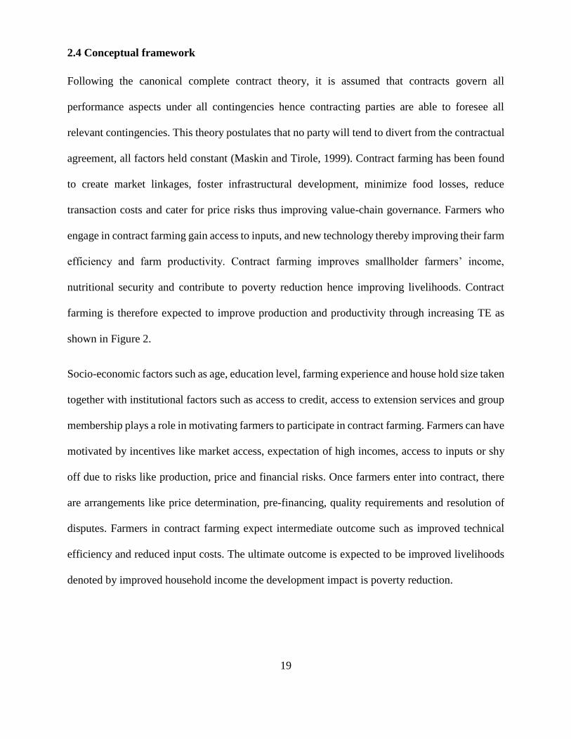
2.4 Conceptual framework
Following the canonical complete contract theory, it is assumed that contracts govern all
performance aspects under all contingencies hence contracting parties are able to foresee all
relevant contingencies. This theory postulates that no party will tend to divert from the contractual
agreement, all factors held constant (Maskin and Tirole, 1999). Contract farming has been found
to create market linkages, foster infrastructural development, minimize food losses, reduce
transaction costs and cater for price risks thus improving value-chain governance. Farmers who
engage in contract farming gain access to inputs, and new technology thereby improving their farm
efficiency and farm productivity. Contract farming improves smallholder farmers’ income,
nutritional security and contribute to poverty reduction hence improving livelihoods. Contract
farming is therefore expected to improve production and productivity through increasing TE as
shown in Figure 2.
Socio-economic factors such as age, education level, farming experience and house hold size taken
together with institutional factors such as access to credit, access to extension services and group
membership plays a role in motivating farmers to participate in contract farming. Farmers can have
motivated by incentives like market access, expectation of high incomes, access to inputs or shy
off due to risks like production, price and financial risks. Once farmers enter into contract, there
are arrangements like price determination, pre-financing, quality requirements and resolution of
disputes. Farmers in contract farming expect intermediate outcome such as improved technical
efficiency and reduced input costs. The ultimate outcome is expected to be improved livelihoods
denoted by improved household income the development impact is poverty reduction.

20
Figure 2: Illustration of farmers’ motivation for contract farming and implications on
livelihoods
Source: Author’s conceptualization.
Incentives
Market access
Expected high
incomes
Access to inputs
Price determination
Technical support
Pre-financing
Standard
requirements
(Quality and
quantity)
Dispute resolution
Socio-
economic
factors (Age,
education
level, farming
experience,
household
size)
Institutional
factors
(Credit,
extension
services,
group
membership)
Livelihoods
Improved
household income
Risks
Production risks
Price risks
Financial risks
Technical
Efficiency
Reduced Input
costs (Labor,
seeds, fertilizer)
Improved Output
Motivation for
contracts
Contract
arrangement
Ultimate
Outcome
Development impact
Poverty
reduction
Intermediate
Outcome

21
2.5 Theoretical framework
This study is anchored on three key theories: convention, agency and agricultural household
theories.
2.5.1 Convention theory
This theory focuses on product attributes. In markets with perfect information, the price reflects
the quality attributes. There are several types of coordination in conventional theory for instance:
industrial, market, domestic and civil coordination. In industrial coordination, one independent
party is responsible for setting threshold. Market coordination on the other hand is characterized
by specific quality conventions that regulate exchange. Domestic coordination is based on trust
and building long-term relationships while civil coordination calls for all firms to come together
and set quality standards to reduce and avoid conflicts (Young and Hobbs, 2002). This theory was
used to analyze motivation for contract farming and factors that lead to violation of the contracts
by incorporating the institutional factors.
2.5.2 Principal-agent theory
Agency theory explains relationships among actors in a given context. It describes the relationship
between principals or agents and delegation of control. It gives strategies to best structure
relationships where one party determines what is to be done and the other performs decisions on
behalf of the principal (Belot and Schroder, 2013). This theory forms the basis for showing
relationships between contracted farmers and firms.
Boland and Marsh (2006) point out that it is difficult to account for uncertainties in contracts;
hence, this increases transaction costs as a result. Uncertainties could be caused by climate change
and other production shocks in agriculture. This implies that there is a possibility of opportunism
between the parties involved in a contract especially after the contractual period. The level of

22
agents’ efforts is concealed by the uncertainties and the principals may suffer from information
asymmetry hence there is likelihood of the agents exploiting the principal.
Uncertainty and information asymmetry result into two main types of agency problems, which are
moral hazard and adverse selection. Moral hazard implies that in any contractual agreement, one
party has the opportunity to gain by choosing not to observe the agreement principles. Moral
hazard means that one party might choose to take higher risks knowing that the other party will
bear the costs of the risks. Adverse selection is a situation whereby there exists asymmetric
information on the agent’s side and the principal lacks information making it difficult to make an
accurate determination of whether the agent is adhering to the contractual agreement by
performing what they are facilitated and will be paid for.
2.5.3 Agricultural household model
Following Azam (2012), this study employed agricultural household model whereby it is
considered that a household produces a variety of output to consume and/or market. A household
is thus faced with utility maximization problem. Rationally, a household maximizes utility by
going for goods at a level where they produce (Qi); using inputs (Xi), consume (Ci), buy (Ni) and
sell (Si). The household is thus required to maximize utility subject to several constraints for
instance production technology, income and resources. Following the assumption that markets are
perfect (with zero transaction costs), the household will have the following constrained
optimization problem.
Max u (Ci,Zc) ……………………………………………………………………………….(1)
Subject to:

23
Income constraint …………………………………...…...(2)
Qi+ E+ N≥ Xi +Ci + Si Resource constraint ...………………………………………..(3)
G(Q, X,Zq) =0 Production technology constraint…………………………...(4)
Ci, Qi, Xi, Ni, Si ≥0 Non-negativity constraint…….………………………………(5)
where:
m
iP represents the market price, iE denotes household endowment in a good, B is the exogenous
income, cZ denotes household attributes and qZ represents technology attributes.
The income constraint (Equation 2) states that total transfers and revenue should be greater or
equal to expenditures. The resource constraint (Equation 3) shows that the quantities of goods used
as inputs, consumed, and sold should not be more than the total amount of output produced. The
production constraint (Equation 4) shows the kind of technology used in production, which is the
interaction of inputs and outputs.
Contracts as institutions are markets by nature and therefore the current study employs this theory
to explore farmers’ choice of market channels to sell produce in the pursuit of utility maximization.
This study uses efficiency as a measure that fits in this theory whereby technology gaps are
computed across farms to compare how farmers in contract and those not in contracts combine
their inputs in the production process. Markets (contracts included) are not perfect in the real world
thus, regardless of the quantity of goods marketed; households incur transaction costs during
participation in markets.

24
CHAPTER THREE: CHARACTERIZATION OF CHILI AND SPIDER PLANT
FARMERS IN WESTERN KENYA
3.1 Abstract
This chapter characterizes chili and spider plant farmers in Western Kenya and is based on
qualitative and quantitative data collected from 300 smallholder chili and spider plant farmers in
Bungoma and Busia counties. Respondents who comprised producers of chili pepper and spider
plant were sampled using multi-stage sampling procedure. The descriptive analysis was done using
STATA software and results presented in tables and charts. The pooled for the two counties results
showed that women dominate in vegetable production at 63%. The pooled data for the two counties
also show that about 60% of the vegetable farmers accessed agricultural extension services with
the proportion being almost the same in Bungoma and Busia counties. Less than half of the
respondents (39%) accessed agricultural credit. The low level of access to credit could be attributed
to poor institutional arrangements and lack of collateral. About half of the respondents participated
in chili and spider contract farming. The findings showed that, for both chili and spider plant, the
proportion of farmers who accessed agricultural credit was two-thirds for both contract participants
and non-participants. The difference is attributed to the fact that contractors offer credit to the
contracted farmers in terms of farm inputs for instance seeds, agro-chemicals and fertilizer.
Contrary to expectation, the proportion of vegetable farmers who accessed agricultural extension
services was lower among contract participants (55%) compared to non-participants (65%).
Slightly over one-third of contracted chili and spider plant farmers are motivated to participate in
contract farming by expectation of an assured market.
Key words: Smallholder farmers, chili, spider plant, contract farming.
25
3.2 Introduction
Vegetables contribute significantly to the Kenyan horticultural GDP. However, vegetable farmers
still face various constraints during production and marketing. Such constraints are; high
production cost due to high input costs, unstable markets for both inputs and outputs, low prices
for outputs, poorly developed infrastructure, inadequate market information due to high
transaction costs, limited access to financial resources, and weak institutional environment.
Moreover, malnutrition is a key challenge in Western Kenya where for instance about half of the
children under 5 years lack a diversified diet (World Bank, 2016). Both chili and spider plant are
rich in vitamins and minerals, hence important components for a nutritionally diversified diet.
African Indigenous Vegetables (AIVs) are also considered more nutritious than exotic vegetables.
Chili and spider plant have shorter growing cycles compared to other major crops like maize.
Extant literature reveals that traditional vegetables give the smallholder farmers a relatively higher
return per unit area than other major crops. Participating in horticultural inclusive value chains can
provide an important link between the rural farmers and the global economy where local suppliers
interact with global institutional buyers in trading fresh produce for instance, fruits and vegetables
(Byerlee et al., 2009). African indigenous vegetables are rich in vitamins and minerals, hence
important components for a nutritionally diversified diet (Ochieng et al., 2016). Such vegetables
have shorter growing cycles as compared to other major crops like maize and they are able to make
maximum utilization of soil nutrients and scarce water supplies (Weinberger and Lumpkin, 2007).
Empirical evidence reveals that AIVs give smallholder farmers higher returns per unit area as
compared to other crops like maize (Afari-Sefa et al., 2015). Some AIVs for instance, the spider
plants are also known for their ease of cooking, production and processing (Kansiime et al., 2016).
The AIVs also have medicinal value and are highly nutritious (Ngenoh et al., 2019). In Bungoma
county for instance, spider plant is grown under 358 ha and spider plant 164 ha Agricultural
26
activities account for about 60% of all the economic activities contributing to gross county product
in Bungoma County, of which vegetables contribute about 30%.
3.3 Methodology
Data was collected from a survey of chili and spider plant farmers in Bungoma and Busia counties
in Western Kenya. Bungoma and Busia counties were purposively selected because of the high
agricultural potential in the region and their strategic geographical position at the boarder of Kenya
and Uganda, as they are potential avenues for improving cross-border trade. Contract farming is
an upcoming institutional arrangement in this area hence it is of interest to know factors
determining its uptake and its effect on livelihoods.
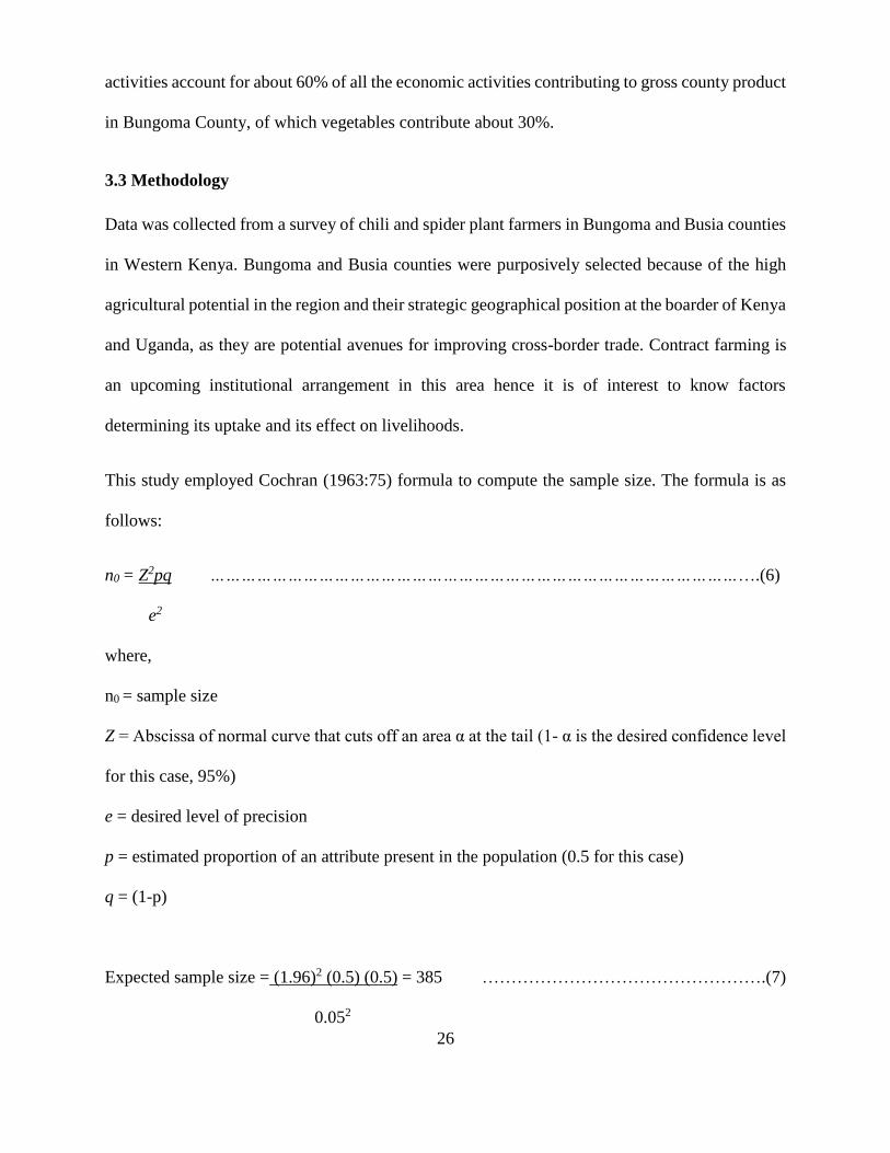
This study employed Cochran (1963:75) formula to compute the sample size. The formula is as
follows:
n0 = Z2pq …………………………………………………………………………………………….(6)
e2
where,
n0 = sample size
Z = Abscissa of normal curve that cuts off an area α at the tail (1- α is the desired confidence level
for this case, 95%)
e = desired level of precision
p = estimated proportion of an attribute present in the population (0.5 for this case)
q = (1-p)
Expected sample size = (1.96)2 (0.5) (0.5) = 385 ………………………………………….(7)
0.052

27
Eventually, the present study ended up using a sample size of 300 instead of the expected 385
vegetable farmers because 85 incomplete questionnaires were removed due to missing crucial data
for key variables such as input use and income, which form the basis of this study leading to a 78%
valid response rate.
A multistage sampling procedure (Bakshi et al., 2019) was used in the selection of the respondents.
First, two sub-counties, Bumula and Matayos were purposively selected in Bungoma and Busia
counties respectively due to the reasonable concentration of chili and spider plant farmers. The
two counties were also selected due to their strategic geographic location at the Kenya-Uganda
boarder that provides an opportunity for cross-border trade in the two value chains. Despite the
fact that there are other areas like central Kenya where contract farming is much common, these
counties were of interest in order to observe how vegetable farmers pick up contracts, even if it is
a new institutional arrangement. In the second stage two wards were selected from each sub-county
using simple random sampling, the third stage had two villages selected from each ward using
simple random sampling method. In the fourth stage, contracted farmers were selected from lists
provided by farmers’ field school (FFS) officers from each sub-county using systematic random
sampling method; where every second responded was selected. The list for Bumula sub-county
had 225 contracted farmers while that for Matayos had 90. A total of 110 and 39 contracted farmers
were selected from Bumula and Matayos sub-counties, respectively. Non-contracted farmers were
selected from a sampling frame provided using systematic random sampling method where every
second and fifth respondent was interviewed. Selection of both participants and non-participating
farmers from the FFS lists could be a source of bias hence future studies should work to overcome
this weakness by diversifying sampling frames for the treatment and control groups.
28
It is important to note that, there were several contracting firms in the study area but they all had
similar contractual terms of delivering inputs upfront, offering support services and buying the
crop at relatively close prices. The contracting firms included; exporters, supermarkets, institutions
like schools and hotels and domestic traders such as hotels. The exporting companies included
MACE foods, which contracts farmers in both Busia and Bungoma counties and exports
vegetables to Europe; schools include Bungoma High School and Cardinal Otunga Girls High
school; supermarkets include Tesia and Khetias supermarkets and hotels include Tourist hotel in
Bungoma. This implies that there was no heterogeneity in contracting firms to affect the
smallholder farmer’s decision to participate in contract farming. In addition, farmers’ field school
members were farmers producing vegetables, including chili and spider plant, besides poultry.
Though not all members of field schools were contracted, there was a clear documentation of the
market channels for the members since the field schools also link their members to markets.
The study also employed a combination of participatory approaches, specifically key informant
interviews and a focus group discussion (FGD). The informant interviews involved consultations
with 4 input suppliers, 2 agricultural extension officers, 2 value addition experts and 2 local
administrators summing up to 10 participants. This was useful in obtaining insights on evolution
of contracts and other production techniques over the years. An FGD was conducted to capture
trends in challenges, opportunities and their drivers along the vegetable value chain. The
stakeholders involved in the FGD included; 2 input suppliers, 2 producers of vegetables, 1 private
and 1 government extension officer, 1 broker, 1 farm laborer, 2 vegetables assemblers, 1 distributor
of vegetables, 1 value addition expert, 1 local administrator, 1 vegetables trader and 1 vegetable
consumer making a total of 15 participants. Focus group discussion enhances a broader perspective
of the research issues and eliminates individual bias in data collection (Boateng, 2012). The aim

29
of the FGD was to get insights concerning the determinants of participating in contract farming,
its effects on farm efficiency and income. The information from the FGD was used in restructuring,
designing and reviewing the survey questionnaire as well as capturing the thoughts and opinions
about the issues in the study.
Semi-structured questionnaires were used for collecting primary data. The questionnaire had five
major sections. First, questions on household identification, then the second section had questions
on land ownership and vegetable production including input use. The third section had questions
concerning vegetable marketing, the fourth section dealt with institutional support with questions
on social capital and extension services. Finally, the last section had questions on livelihoods and
socio-demographic aspects. Minhat (2015) considered semi-structure questionnaire suitable
because of its flexibility in giving enumerators a chance to validate the responses and probe for
clarification where possible.
3.4 Results and discussion
3.4.1 General socio-economic characteristics of vegetable farmers in Bungoma and Busia
Table 1 shows the characteristics of farmers growing vegetables in Bungoma and Busia counties.
The pooled results reveal that 58% of the respondents were female and 8.7% of the households
were female-headed and these women were widows and single mothers. Female-headed
households were defined as those households whose major decision maker was a female person.
This observation conforms to the low level of female leadership and the power dynamics in African
settings where most of the households are male-headed.

30
Table 1: Characteristics of chili and spider plant farmers in Busia and Bungoma counties
Note: Standard deviations are in parentheses: 1USD = Kshs 101.16 at the time of survey.
Source: Survey Data (2019).
Women get involved in subsistence agriculture for instance vegetable production due to gender
roles within the rural households. Bungoma county has a higher proportion of female-headed
households compared to that of Busia. From the focus group discussions, some of the female-
headed households were attributed to death of male heads and family break-ups. The pooled
results reveal that 87% of the vegetable farmers use organic fertilizer in vegetable production to
boost yield. This could be an evidence of a decline in soil fertility hence there is need to replenish
the soil and increase the level of soil nutrients through use of fertilizer. The proportion of farmers
Variable Bungoma (a)
(n = 201)
Busia (b)
(n = 99)
Pooled
(n = 300)
Test of
statistically
significant
differences
Categorical Variables χ2 test
Gender of the farmer (% male) 62.7 48.5 58.0 0.019**
Household type (% female-headed) 10.5 5.0 8.7 0.118
Fertilizer use (% yes) 87.5 85.8 87.0 0.680
Membership to agricultural
development group (% yes)
55.7 69.7 60.3 0.020**
Farmer’s access to extension (% yes) 59.2 60.6 59.7 0.816
Farmer’s access to credit (yes %) 35.8 45.5 39.0 0.100*
Participation in contract
farming (% yes)
54.7 39.4 49.6 0.013**
Type of vegetable (% Chili) 43.8 39.4 42.3 0.470
Continuous variables t-test
(a-b)
Average years of formal education of
the farmer
9.1(3.6) 8.5(4.3) 8.9 (3.8) 0.093
Average age of the farmer (years) 48(14) 50(13) 49 (14) -0.053
Distance from home to market (Kms) 3.7(3.8) 3.7(1.6) 3.8(3.2) -0.066
Average total land size (acres) 3.0(5.2) 2.6(1.7) 2.9(4.4) -0.064
Average years of farming experience 8.7(9.0) 10.6(10.3) 9.3(9.5) 0.284**
Average on-farm income (Kshs) 7,379(5,540) 7,574(5,202) 7,453(5,422) 0.005
Average off-farm income (Kshs) 1,848(1,385) 1,893(1,300) 1,863(1,355) -45.410

31
using fertilizer use is almost equal in both counties. About 60% of the vegetable farmers are
members of agricultural development groups.
The proportion of farmers in agricultural development groups in Busia is higher compared to that
of Bungoma. This is explained by the fact that there was low concentration of agricultural
development groups in part of Bungoma though contracts are active. Studies such as
Frankenberger et al. (2013) reveal that farmers who are members of agricultural development
groups gain access to inputs and group credits to improve their production. Membership to
agricultural groups also improves access to market linkages and provides an avenue to lobby for
better produce prices by increasing farmers’ bargaining power due to their ability to control
volumes. This is consistent with some other studies for instance, Franken et al. (2014) who found
a positive relationship between social capital and access to high value markets.
The pooled data also shows that about 60% of the vegetable farmers accessed agricultural
extension services in form of training. Access to agricultural extension services increases
dissemination of agricultural knowledge and farming technology, which helps farmers to improve
their productivity. In addition, increasing extension services among smallholder producers,
increases chances of market linkages (Quisumbing and Pandolfelli, 2010). Access to agricultural
extension service was measured by whether the farmer actually received technical advice from
private or government extension officers.
Less than half of the respondents (39%) accessed agricultural credit. The proportion of farmers
who accessed agricultural credit is higher in Busia than Bungoma. The low level of access to credit
could be attributed to lack of collateral to secure credit. In most cases, various lenders use land
title deed as a requirement for credit. Fischer and Qaim (2012) asserted that the low access to
agricultural credit services is caused by the need for collateral by formal lending institutions.

32
Access to agricultural credit was defined as whether the farmer actually received credit in cash or
inputs.
For the years of farming experience, the standard deviation was higher than the mean. This implies
that the distribution of the variable was not normal as shown in Figure 3. This is an evidence of
wide distribution of the data among the respondents due to heterogeneity of respondents’
characteristics. As a remedy mode, which is the most appearing number in a data set was used.
Farming experience therefore had a mode of 5 years for the pooled sample. The same applied to
total land size and distance from home to the local market.
Figure 3: Frequency distribution graph for years of farming experience
Source: Survey Data (2019).
About half of the respondents participated in vegetable contract farming. Farmers are motivated
to participate in contract farming by the desire to access farm inputs in form of credit, acquire
technical know-how and stable market for their produce (Bellemare, 2012; Sokchea and Culas,
2015; and Bellemare and Novak, 2017). The FGD results show that, low contract prices, lack of
trust, overpricing of services by contractors and delay in payments lead to violation of contracts.
0
10
20
30
40
50
60
70
80
0-10 10-20 20-30 30-40 40-50 50-60
Per
cent
of
farm
ers
Average years of farming experience

33
The respondents had an average of about 9 years of formal education implying that they had at
least attained basic primary literacy levels useful for understanding the terms of the contracts.
The average age of the respondents was 49 years. The pooled results indicate that the average
distance from the farm to the nearest open air market is 3.8 kilometers. However as explained
earlier, the standard deviation was higher than the mean and the distribution was not normal as
shown in Figure 4. The modal distance to the nearest market for the pooled sample was 3
kilometres.
Figure 4: A frequency distribution graph for distance from home to the nearest local market
Source: Survey Data (2019).
This implies that farmers have to move longer distance to deliver their produce to the main market,
hence perishability and high transport costs sets in unless the buyer picks from the farm.
Results from the FGD revealed that, the major sources of extension services were farmer-to-farmer
extension, government extension officers, contracting firms, researchers and media. Contrary to
expectation, the proportion of vegetable farmers who accessed agricultural extension services was
lower among contract participants compared to non-participants. The contracting companies or
0
10
20
30
40
50
60
70
80
90
100
0-10 10-20 20-30 30-40
Per
cent
of
farm
ers
Average distance to the market
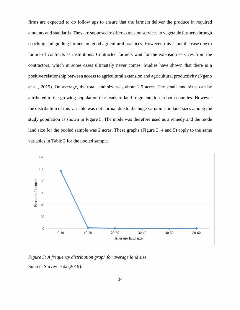
34
firms are expected to do follow ups to ensure that the farmers deliver the produce in required
amounts and standards. They are supposed to offer extension services to vegetable farmers through
coaching and guiding farmers on good agricultural practices. However, this is not the case due to
failure of contracts as institutions. Contracted farmers wait for the extension services from the
contractors, which in some cases ultimately never comes. Studies have shown that there is a
positive relationship between access to agricultural extension and agricultural productivity (Ngeno
et al., 2019). On average, the total land size was about 2.9 acres. The small land sizes can be
attributed to the growing population that leads to land fragmentation in both counties. However
the distribution of this variable was not normal due to the huge variations in land sizes among the
study population as shown in Figure 5. The mode was therefore used as a remedy and the mode
land size for the pooled sample was 2 acres. These graphs (Figure 3, 4 and 5) apply to the same
variables in Table 2 for the pooled sample.
Figure 5: A frequency distribution graph for average land size
Source: Survey Data (2019).
0
20
40
60
80
100
120
0-10 10-20 20-30 30-40 40-50 50-60
Per
cent
of
farm
ers
Average land size

35
3.4.2 Comparison of socio-economic characteristics of spider plant and chili farmers
Table 2 below shows the socio-economic characteristics of spider plant and chili farmers. It was
revealed that there was a higher proportion of female farmers growing chili (66.1%) compared to
that growing spider plant (52%). For both vegetables, the proportion of female-headed households
is very low (8.6% for spider plant and 8.7% for chili).
The proportion of farmers who use fertilizer is higher among chili farmers (92.9%) than spider
plant (82.6%). This could be attributed to the difference in the nutritional requirements of chili and
spider plant and the need to improve chili yield to meet contractors’ standards. There is no
significant difference in the proportion of membership to agricultural development group among
chili and spider plant farmers. Farmers growing chili have a higher access to credit (43%)
compared to those growing spider plant (35%). This is because most of the farmers growing Chili
participate in contract farming which to some extent increases their access to credit in form of farm
inputs (Rao and Qaim, 2011).
Slightly more than half (55%) of the farmers growing chili participate in contract farming
compared to only 45% of spider plant farmers. This is explained by the fact that most contracting
firms in the study area have a higher demand for chili than spider plant. The average number of
years of completed formal education is higher (9.4) among chili farmers compared to spider plant
(8.5). The level of formal education is directly related to effective utilization and combination of
production resources and rational decision making to maximize output. The average level of
experience of farmers growing spider plant is higher (10.1) compared to that of spider plant farmers
(8.4). The more the years of experience, the more the farmers have technical skills about the crop
they are producing.

36
Table 2: Socio-economic characteristics of spider plant and chili farmers
Note: Standard deviations are in parenthesis: 1USD = Kshs 101.16 at the time of survey.
Source: Survey Data (2019).
Chili farmers earn an average of Kshs. 8,586 (USD 84.95) on-farm income per season that is higher
compared to that of spider farmers, Kshs. 6,620 (USD 65.51). This indicates that chili is a higher
value crop compared to spider plant. On the other hand, for both chili and spider plant farmers, the
proportion of those who accessed agricultural credit was slightly higher among contract
participants (62%) compared to non-participants (60%). The difference is attributed to the fact that
contractors offer credit to the contracted farmers in terms of farm inputs for instance seeds, agro-
chemicals and fertilizer. Farmers participating in contracts are likely to achieve high productivity
and welfare gains (Barrett et al., 2012; Ma and Abdulai, 2016). Farmers who do not participate in
Variable Spider plant
(n = 173)
Chili
(n = 127)
Pooled
sampler
(n = 300)
Test of
statistically
significance
differences
Categorical Variables χ2 test
Gender of the farmer (% male) 52.0 66.1 58.0 0.014**
HH type (% female-headed) 8.6 8.7 8.7 0.998
Fertilizer use (% yes) 82.6 92.9 87.0 0.009***
Membership to agricultural
development group (% yes)
60.1 60.6 60.3 0.928
Access to agricultural extension (% yes) 59.4 59.8 59.7 0.958
Access to credit (% yes) 35.84 43.3 39.0 0.190
Participation in contract
Farming (%yes)
45.6 55.1 49.6 0.100*
Continuous variables t-test (a-b)
Average years of formal education 8.5(4.1) 9.4(3.3) 8.9 (3.8) -0.189***
Average age (years) 49.0(14.0) 47.0(13.0) 49.0(14.0) 0.039
Distance to market (Km) 3.6(2.3) 4.2(4.1) 3.8(3.2) -0.020
Average land size (acres) 2.9(5.1) 2.8(3.1) 2.9(4.4) -0.041
Average years of farming experience 10.1(10.4) 8.4(8.2) 9.3(9.5) 0.170*
Average on-farm income (Kshs) 6,620(5,111) 8,586(5,645) 7,453(5,422) -0.245***
Average off-farm income (Kshs) 1,655(1,277) 2,146(1,411) 1,863(1,355) -0.491***

37
contracts have lesser privilege when it comes to accessing agricultural credit that specifically
comes in a contractor’s package.
3.5 Nature of contract farming and farmers’ motivations
3.5.1 Nature of contracts
The proportion of contracted vegetable farmers under formal contracts is higher (64%) compared
to those under informal contracts as shown in Figure 6. Informal contracts involve oral agreements
with no written binding documents. From the FGD, it was revealed that in earlier days (1980s and
1990s), informal contracts were common, they involved oral agreements with relatives, and friends
to provide labor, inputs, buy and sell vegetables. The contract's duration ranged from a week to
several years and the contract terms were rarely violated.
Figure 6: Comparison of nature of contracts between Bungoma and Busia counties
Source: Survey Data (2019).
0
10
20
30
40
50
60
70
80
Bungoma Busia Pooled
Per
cent
of
veg
etab
le s
takeh
old
ers
County
Formal Contracts Informal Contracts
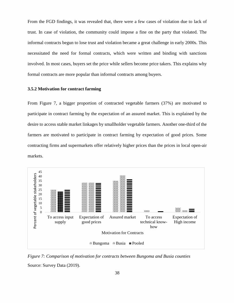
38
From the FGD findings, it was revealed that, there were a few cases of violation due to lack of
trust. In case of violation, the community could impose a fine on the party that violated. The
informal contracts begun to lose trust and violation became a great challenge in early 2000s. This
necessitated the need for formal contracts, which were written and binding with sanctions
involved. In most cases, buyers set the price while sellers become price takers. This explains why
formal contracts are more popular than informal contracts among buyers.
3.5.2 Motivation for contract farming
From Figure 7, a bigger proportion of contracted vegetable farmers (37%) are motivated to
participate in contract farming by the expectation of an assured market. This is explained by the
desire to access stable market linkages by smallholder vegetable farmers. Another one-third of the
farmers are motivated to participate in contract farming by expectation of good prices. Some
contracting firms and supermarkets offer relatively higher prices than the prices in local open-air
markets.
Figure 7: Comparison of motivation for contracts between Bungoma and Busia counties
Source: Survey Data (2019).
0
5
10
15
20
25
30
35
40
45
To access input
supply
Expectation of
good prices
Assured market To access
technical know-
how
Expectation of
High income
Per
cen
t o
f ve
geta
ble
sta
keh
old
ers
Motivation for Contracts
Bungoma Busia Pooled
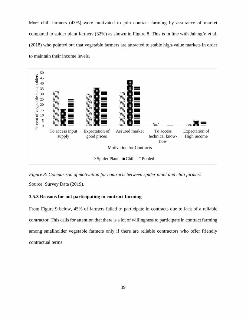
39
More chili farmers (43%) were motivated to join contract farming by assurance of market
compared to spider plant farmers (32%) as shown in Figure 8. This is in line with Jalang’o et al.
(2018) who pointed out that vegetable farmers are attracted to stable high-value markets in order
to maintain their income levels.
Figure 8: Comparison of motivation for contracts between spider plant and chili farmers
Source: Survey Data (2019).
3.5.3 Reasons for not participating in contract farming
From Figure 9 below, 45% of farmers failed to participate in contracts due to lack of a reliable
contractor. This calls for attention that there is a lot of willingness to participate in contract farming
among smallholder vegetable farmers only if there are reliable contractors who offer friendly
contractual terms.
0
5
10
15
20
25
30
35
40
45
50
To access input
supply
Expectation of
good prices
Assured market To access
technical know-
how
Expectation of
High income
Per
cent of
veg
etab
le s
tak
eho
lder
s
Motivation for Contracts
Spider Plant Chili Pooled

40
Figure 9: A comparison of reasons for not participating in contract farming between Bungoma
and Busia counties
Source: Survey Data (2019).
The proportion was higher in Bungoma county compared to Busia county. Production risk was
also reported as a key factor for not participating in contract farming especially in Busia (40%).
Production risks include unreliable rainfall patterns. Drought is becoming a threat in the study area
and so farmers may fear to commit to a contract due to expectation of poor harvest.
Figure 10 below shows similar results among chili and spider plant farmers where lack of
contractor happens to hinder most farmers (43%) from participating in contract farming. This
proportion is higher among spider plant farmers compared to chili farmers. Price risk was found
to be another major hindrance to participation among chili farmers (27%).
0
10
20
30
40
50
60
Producton risks Price risks Financial Risks Lack of contractor
Per
cen
t o
f ve
geta
ble
sta
keh
old
ers
Reasons for not Participating in Contracts
Bungoma Busia Pooled

41
Figure 10: A comparison of reasons for not participating in contract farming between spider
plant and chili farmers.
Source: Survey Data (2019).
Price risks entail fluctuation and volatility in prices whereby at times contractors tend to offer
lower prices than the price existing in the local markets. This discourages farmers from
participating in contracts as it ties them to deliver at lower prices.
3.5.4 Production variables
The main production variables and output for chili and spider plant enterprises are summarized in
Table 3 below.
0
5
10
15
20
25
30
35
40
45
50
Producton risks Price risks Financial Risks Lack of contractor
Per
cen
t o
f re
spo
nd
ents
Reasons for not participating in Contracts
Spider Plant Chili Pooled

42
Table 3: Average annual output and inputs
Source: Survey Data (2019).
The average land sizes for both spider plant and chili farmers is almost the same. The average
hired labor for chili was higher (2.7 man-days) compared to that of spider plant (1.6 man-days).
This implies that chili is more labor-intensive than spider-plant due to the nature of the crop. The
quantity of inorganic fertilizer used is higher among spider plant farmers compared to chili
farmers. This suggests that spider plant has higher nutritional requirements than chili. Table 4
below shows the value of the outputs and variable inputs used in production for both chili and
spider plant farmers.
Variable Spider plant
(n = 173)
Chili
(n = 127)
Output (kgs) 239.5 409.3
Quantity of seeds (kgs) 5.0 0.7
Quantity of inorganic fertilizer (kgs) 63.8 54.9
Hired labor (man-days) 1.6 2.7
Average land size(acres) 2.9 2.8
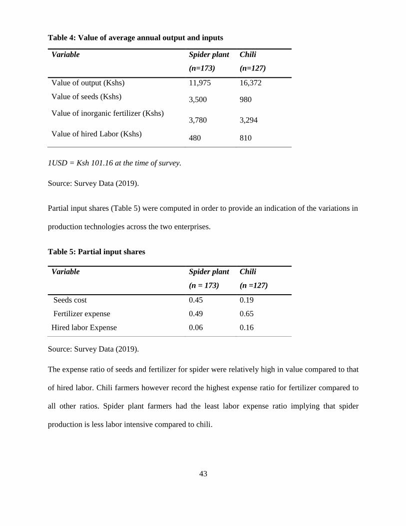
43
Table 4: Value of average annual output and inputs
1USD = Ksh 101.16 at the time of survey.
Source: Survey Data (2019).
Partial input shares (Table 5) were computed in order to provide an indication of the variations in
production technologies across the two enterprises.
Table 5: Partial input shares
Source: Survey Data (2019).
The expense ratio of seeds and fertilizer for spider were relatively high in value compared to that
of hired labor. Chili farmers however record the highest expense ratio for fertilizer compared to
all other ratios. Spider plant farmers had the least labor expense ratio implying that spider
production is less labor intensive compared to chili.
Variable Spider plant
(n=173)
Chili
(n=127)
Value of output (Kshs) 11,975 16,372
Value of seeds (Kshs) 3,500 980
Value of inorganic fertilizer (Kshs) 3,780 3,294
Value of hired Labor (Kshs) 480 810
Variable Spider plant
(n = 173)
Chili
(n =127)
Seeds cost 0.45 0.19
Fertilizer expense 0.49 0.65
Hired labor Expense 0.06 0.16
44
CHAPTER FOUR: DETERMINANTS OF SMALLHOLDER FARMERS’
PARTICIPATION IN CONTRACT FARMING AND ITS FFECT ON INCOME IN
WESTERN KENYA
4.1 Abstract
The transition from selling in spot markets to complex institutional layouts such as contractual
arrangements is viewed as a crucial driver towards structural transformation. In SSA, contract
farming is considered as one of the most effective example of such pattern, both from buyers and
producers’ perspectives. The need to access inputs, market linkages and high incomes are some of
the factors thought to affect participation in contract farming. This study analyzed determinants of
participation in contract farming among vegetable farmers in Western Kenya. The study used both
qualitative and quantitative data. A focus group discussion was conducted to provide information
on the factors that determine farmers’ participation in contract farming and reasons for violation
of contracts. Interviews were conducted with 300 smallholder vegetable farmers using semi-
structured questionnaires. A binary probit model was used to analyze the determinants of
participation in contract farming. A two-step endogenous treatment regression model was used to
analyze the effect of contract farming on farm income. The probit results indicate that distance to
the market place had a positive effect on participation in contract farming for chili farmers and
pooled farmers as well. Land size was found to have a positive influence on participation in
contract farming for both spider plant and pooled farmers. Off-farm income had a positive
influence on participation in contract farming. Results also revealed that membership to
agricultural development groups had a negative influence on participation in contract farming for
both spider plant and pooled farmers. Contrary to expectations, farming experience had a negative
effect on participation in contract farming for spider plant and pooled farmers. Endogenous
treatment regression model results show that participation in contract farming has a positive effect

45
on income for spider plant, chili and pooled vegetable farmers. Public institutions and development
practitioners which purpose to intervene through strengthening contract farming should seek to
understand the dynamics of determinants of participation in order to improve the welfare of
vegetable farmers by improving on-farm incomes.
Key words: Contract farming, chili, spider plant, income.
4.2 Introduction
In developing countries, most of the policies are geared towards increasing agricultural
productivity. This is through increasing the access of smallholder farmers to inputs and the
efficiency in utilization of those inputs. Some institutions for instance contract farming are being
adopted in order to improve smallholder farmers’ efficiency and income. This happens through
the improvement of access to agricultural extension services, agricultural credit, effective and
productive inputs, output markets and better output prices (Bellemare, 2017). Contract farming is
one of the potential strategies for improving the welfare of smallholder farmers through increased
income. Contract farming turns out to be an attractive and viable option for various policy makers
who have an interest in transforming the poor farmers in SSA into industrialized producers by
enabling them get access to significant gains from farms that characterize successful contract
farming.
Despite the perceived benefits of contract farming in developing countries, there has been
documented evidence of violation of farming contracts among smallholder farmers. This study
analyzed the determinants of participation in contract farming in order to provide viable
recommendations to governments and private stakeholders on how best to articulate policies to
strengthen contract framing.

46
There is a thin literature that quantitatively and qualitatively reports on the determinants of
participation in contract farming especially in indigenous vegetables like spider and chili in
specific. For instance, Arumugam (2010) found that there are four important factors determining
farmers’ participation in contract farming. These factors include stability of the market, access to
market information, transfer of production technology that improves farming practices and indirect
benefits. However, the study overlooked individual characteristics and institutional factors. The
present study incorporates important institutional factors such as access to extension services,
access to agricultural credit and social capital membership to agricultural development groups.
The need for market access is a key factor that stimulates the spread of contract farming. The need
to reduce the involvement of the government in provision of services, the growing number of
supermarkets and the high level of interest and attention of donors are the other reasons that explain
why contract farming is becoming more popular. Literature shows that contract farming has a
positive impact on the smallholder farmers by enabling them to gain better access to ready local
markets and global markets. Studies on effect of participating in contract farming for instance,
Bijman (2008) reveal that participating farmers benefit in terms of high incomes. Other scholars
who focused on economic benefits from contract farming to the participants across various value
chains found that contract farming increases the cost of production as well as the gross returns.
This is due to high level of differentiation and high input costs. Some studies also reveal that
contract farming has a negative effect on income. To address the inconclusiveness of the perceived
benefits of contract farming, this study aimed at analyzing the effect of participating in contract
farming on farm income.

47
4.3 Methodology
4.3.1 Estimation of probit model for determinants of participation in contract farming
A probit model was used to analyze factors determining participation in contract farming. The
basic assumption of the probit model is that the error term has normal distribution. A probit model
was chosen over logit due to its normal distribution as compared to logit’s logistic distribution
(Berry et al., 2010). In addition, following Jacque Bera’s test of normality, the probit model was
found to best fit the data.
It is assumed that there is a latent variable 𝑃𝑖∗ that the decides the value of 𝑃𝑖 in that;
𝑃𝑖∗ = 𝛼𝑍𝑖 + 𝜀; ………………………………………………………………………..………. (8)
Where,
𝑃𝑖 = {1 𝑖𝑓 𝑃𝑖
∗ > 0
0, 𝑖𝑓 𝑃𝑖∗ ≤ 0
………………………...………………………………………………… (9)
where 𝑍𝑖 represents a vector of exogenous variables; 𝛼 is a vector of unknown parameters to be
estimated and 𝜀 is a normally distributed error term. The probability that an individual belongs to
a group j is expressed as;
Pr(𝑃𝑖 = 1|𝑍𝑖) =, 𝑓𝑜𝑟 𝑖 = 0, 1 ………………………………………………………... (10)
The parameter estimates of the probit model only indicate the direction of the effect of the
explanatory variables on the dependent variable. The magnitude of the change in the dependent
variable following a unit change in an explanatory variable can be attained by computing marginal
effects of the explanatory variables. The marginal effects are calculated as;
𝜕𝑃((𝑃𝑖 = 1|𝑍𝑖)
𝜕𝑍𝑖=
𝜕𝐸(𝑃𝑖|𝑍𝑖
𝜕𝑍𝑖= 𝜑(𝑍𝑖′𝛽)𝛽………………………………………….………...… (11)

48
The regression model was empirically estimated as shown below;
Yi= βo +β1 X1i+ β 2 X2+ β 3 X3 + β 4 X4 + β 5X5+ β 6X6+ β 7X7+ β 8X8+ β 9X9+ β 10X10 +Ԑ .…(12)
where,
Y = Participation in contract farming (1 = yes, 0 = No)
X1 = Age of the farmer (years)
X2 = Total land size (ha)
X3 = Farming experience of the farmer (years)
X4 = Level of formal education of the farmer (years)
X5 = Membership to agricultural development group by the farmer (1 = yes, 0 = No)
X6 = Off-farm income of the household (Kshs)
X7 = Distance from home to the market (Km)
X8 = Gender of the farmer (1 = male, 0 = female)
X9 = Farmer’s access to agricultural credit in the last one year (1 = Yes, 0 = No)
X10 = Farmer’s access to agricultural extension (1 = yes, 0 = No)
Ԑ = The error term

49
4.3.2 Expected signs of variables for determinants of participation in contract farming
Table 6 below shows the expected signs of determinants of participation in contract farming.
Table 6: The expected signs of determinants of participation in contract farming
Variable Description of the variable Expected sign
X1 = Age Age of the farmer involved in production
and marketing of the target crop in years
+/-
X2 = Land size Total land size owned in acres +
X3 = Farming experience Farming experience of the farmer
involved in production and marketing of
the target crop
+
X4 = Level of education Years of formal education of the farmer
involved in production and marketing of
the target crop
+
X5 = Membership to group Dummy(1=Yes,0 = No) +
X6 = Access to formal
agricultural credit
Dummy(1=Yes,0 = N0) +
X7 = Access to government
extension
Dummy(1=Yes,0 = N0) +
X8 = Gender of the farmer Dummy(1=Yes,0 = N0) +/-
X9 = Off-farm income Off-farm income of the household in Kshs +
X10 = Distance to the market Distance from home to the nearest local
market in Km
+/-
X11 = Household size Number of members living in a household +/-
X12 = Household type Male-headed or female-headed
household
+/-
Source: Survey Data (2019).
Age was expected to have either negative or positive effect on participation in contract farming
due to the inconclusively of previous findings. Gender was expected to have either negative or
positive effect on participation in contract farming due to documented variations in preferences
for contract farming among males and females. Farming experience was expected to be positive

50
since farmers who have been in farming for long have a better perception of benefits of contract
farming and are well acquainted with risk management skills (Barrett et al., 2012). The level of
education was expected to have a positive sign since it plays a key role in improving the quality
of decisions that are made by the farmer and act as an empowerment tool (Abdallah, 2016). The
more educated a farmer is the more likely he is to embrace innovations such as contract farming.
Access to agricultural credit was expected to have a positive effect on contract farming since most
farmers in SSA are resource-poor and would go for any interventions or opportunities that enable
them to access credit for to fund production (Arumugam et al., 2011). The effect of access to
agricultural extension was also expected to be positive according to Barret et al. ( 2011). This is
because, some contractual arrangements are in a way that the contracting party offers extension
services through making farm visits and offering technical advice. Off-farm income was expected
to have a positive sign due to the relationship between financial stability and the capacity to
participate in contract farming.
Land size owned was expected to have a positive effect on participation in contract farming due
to motivation to meet the buyers’ demand. Distance from home to the nearest market is expected
to have a positive sign following the findings of Narrod et al. (2009) and Trebbin (2014). This is
owed to the fact that the longer the distance the more willingness of the farmer to go for higher
value markets such as contract farming to save on transportation costs especially when the
contractor covers transport costs. Both household size and household type were expected to have
either negative or positive effect on contract farming due to varied views laid out in previous
literature.

51
4.3.3 Endogenous treatment effect regression model for effect of contract farming on
income
A two-step Endogenous Treatment Regression Model was applied because the purpose of the
model is to estimate the effect of undergoing treatment while accounting for its endogeneity and
selection bias (Vella, 2011). To control for endogeneity and selection bias, the control function
makes use of two steps estimation procedure. The model would make use of the predicted
probability of participation in contract farming on obtained in the first step in equation 13 to
estimate the effect of contract farming on income in equation 14. The decision to participate in
contract farming is estimated as a selection equation (13) in the first step to generate the control
function. The control function is thereafter included as one of the explanatory variables
representing the predicted probability of participating in contract farming in the second step in
equation 14.
A binary probit model was used to estimate the first step and the second step was regressed using
predicted value from the first stage. From the theoretical model, there must be factors that
determine choice of a production intervention, and then decisions on consumption level follow
based on the effect of the intervention on productivity whose proxy is income in this case. The
beginning of the empirical analysis is therefore a two-stage approach as shown below:
𝑃𝑖∗ = 𝛼𝑍𝑖 + 𝜀; ………………………………………………………………………..…. (13)
𝑋𝑖 = 𝛽𝑌𝑖 + 𝜓𝑃𝑖 + 𝑒𝑖 ……………………………………………………………….…. (14)
Equation (13) is the first step showing determinants of participation in contract farming and
equation (14) illustrates the effect of participation in contract farming among other factors on
income (second step).

52
where, 𝑃𝑖 is participation in contract farming, captured as a dummy variable indicating whether
or not a household participated in contract farming; 𝑋𝑖 is the level of household income. The
vectors 𝑍𝑖 𝑎𝑛𝑑 𝑌𝑖 represent exogenous factors hypothesized to affect participation in contract
farming, and income levels, respectively. The unknown parameters to be estimated are 𝛼, β, 𝑎nd
ψ; while 𝜀𝑖, and 𝑒𝑖 represent error terms of the respective equations.
A binary probit model was applied in this first step because the dependent variable, participation
in contract farming (𝑃𝑖) was binary; coded as one (1) and zero (0) for ‘yes’ and ‘no’ responses
respectively. The second step (Equation 14) aimed at obtaining the predicted estimates of factors
affecting income, participation in contract farming included. Ordinary least squares (OLS) was
applied as it is suitable for investigating issues that are cross-section in nature. It is crucial to note
that interactions between 𝑋𝑖 and 𝑃𝑖 are allowed in equation 14.
Previous studies have used aggregate income from on farm activities. However, this study used
income from target crops, that is spider plant and chili whereby gross margins were calculated for
each value chain where the production costs (input costs) was deducted from the total revenue
from sale of chili and spider plants to get of farm income for chili and spider plant.
4.3.4 Expected signs of variables for the endogenous treatment regression model
Table 7 shows expected signs of factors affecting income of vegetable farmers. Participation in
contract farming was expected to have either negative or positive sign given that previous studies
found inconclusive results. For instance Ballamere (2017) found a positive sign for participation
in contract farming while others such as Von Hagan and Alvarez (2011) found a negative sign.
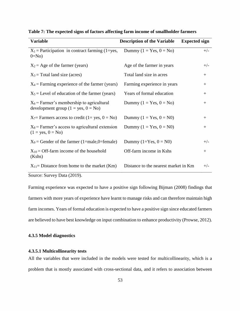
53
Table 7: The expected signs of factors affecting farm income of smallholder farmers
Variable Description of the Variable Expected sign
X1 = Participation in contract farming (1=yes,
0=No)
Dummy (1 = Yes, 0 = No) +/-
X2 = Age of the farmer (years) Age of the farmer in years +/-
X3 = Total land size (acres) Total land size in acres +
X4 = Farming experience of the farmer (years) Farming experience in years +
X5 = Level of education of the farmer (years) Years of formal education +
X6 = Farmer’s membership to agricultural
development group (1 = yes, 0 = No)
Dummy (1 = Yes, 0 = No) +
X7= Farmers access to credit (1= yes, 0 = No) Dummy (1 = Yes, 0 = N0) +
X8 = Farmer’s access to agricultural extension
(1 = yes, 0 = No)
Dummy (1 = Yes, 0 = N0) +
X9 = Gender of the farmer (1=male,0=female) Dummy (1=Yes, 0 = N0) +/-
X10 = Off-farm income of the household
(Kshs)
Off-farm income in Kshs +
X11= Distance from home to the market (Km) Distance to the nearest market in Km +/-
Source: Survey Data (2019).
Farming experience was expected to have a positive sign following Bijman (2008) findings that
farmers with more years of experience have learnt to manage risks and can therefore maintain high
farm incomes. Years of formal education is expected to have a positive sign since educated farmers
are believed to have best knowledge on input combination to enhance productivity (Prowse, 2012).
4.3.5 Model diagnostics
4.3.5.1 Multicollinearity tests
All the variables that were included in the models were tested for multicollinearity, which is a
problem that is mostly associated with cross-sectional data, and it refers to association between

54
the independent variables. This leads to the widening of the confidence interval and unreliability
of the inferences due to the inflation of the variance of coefficients and the model in general.
The multicollinearity test was conducted by use of variance inflation factor (VIFs) shown in
equation 15 and partial correlation analysis.
𝑉𝐼𝐹𝑖 =1
1− 𝑅𝑖2 ……………………………………………..……………………………….…. (15)
where, 𝑅𝑖2is the multiple R2 for the regression of a variable on the other covariates.
According to Gujarati and Porter (2009), VIF values above 5 indicates that there is evidence of
severe multicollinearity. The models did not have any evidence of multicollinearity as shown in
Appendices 2 and 3.
In order to further rule out correlation, a partial correlation test was conducted for the Endogenous
Treatment Regression Model. Partial correlation is the measure of association between two
variables, while controlling or adjusting the effect of one or more additional variables. Partial
correlation analysis explores the linear relationship between two variables after excluding the
effect of one or more independent factors (Baba et al., 2004). The results showed that there was
no serious correlation as the magnitude of all the correlation of all the variables were below 0.5 as
shown in Appendix 4.

55
4.3.5.2 Heteroscedasticity
Heteroscedasticity is the variance of the error term varying across observations and results in
inefficient estimators, incorrect confidence interval and incorrect t-statistics in linear regression. The
Breusch-Pagan/Cook-Weisberg test was applied in testing for the presence of heterogeneity in the
Endogenous Treatment Regression Model. There was no presence of heteroscedasticity in the two
steps.
4.3.5.3 Test for poolability of data from Bungoma and Busia counties
The Chow test was employed in testing for poolability to determine whether to pool the data or split
it into individual counties during data analysis. Chow test was calculated as shown below:
………………………………….. (16)
where,
RSSp is the residual sum of squares for the pooled regression model, RSS1...n is the Residual Sum of
squares for the regression model of the split data, K is the degrees of freedom and N is the sample size
for the pooled sample.
In this test, the F calculated values are compared with the F critical values. The null hypothesis that
data can be pooled in a single regression is rejected when the F calculated value is greater than the F
critical value. This leads to splitting of the data and analysis of sub-samples.
In this study, the F calculated value for the farmers’ probit model was 0.978. This showed that
estimating the regression with pooled data had significant improvement in the model; hence, separate
models for contract participation in the two counties are not presented and thus subsequent discussions
are based on the pooled model, though with a county dummy variable. This is consistent with the

56
observations of Barasa et al. (2018) in their malnutrition management study in Busia and Bungoma
that there are no statistical differences in the farmer characteristics in the two counties.
4.4 Results and discussion
4.4.1 Results and discussions for probit model
Table 8 below shows results from the binary probit regression model on for determinants of
participation in contract farming. Distance to the market, total land size, and off-farm income were
found to positively influence participation in contract farming. The distance to the market place had a
positive influence on participation in contract farming for Chili farmers and to pooled farmers as well.
This is attributed to the fact that the farmers are motivated because of savings on transportation costs
especially when the buyer comes to pick the produce. Narrod et al. (2009) and Trebbin (2014) also
found that distance had a positive relationship with access to high–value markets.
Contrary to the expectation, farming experience had a negative effect on participation in contract
farming for spider plant farmers and pooled farmers. As indicated by the findings from the FGD
farmers with more farming experience are reluctant to embrace new technology including contract
farming, which is an institutional innovation. On the other hand, farmers with less farming experience
have high expectations and interest in trying out new ways of farming as part of exploration.

57
Table 8: Factors influencing farmers’ participation in contract farming in Western Kenya
Significance levels: *** 1%; ** 5%; * 10%.1USD = Kshs 101.16 at the time of survey
Source: Survey Data (2019).
Spider plant
(n = 173)
Chili
(n = 127)
Pooled sample
(n = 300)
Variable Coefficient RSE Coefficient RES Coefficient RES dy/dx
Distance from home to the market (Kms) 0.401 0.348 0.466** 0.234 0.379** 0.175 0.111
Farming experience of the farmer (years) -0.407*** 0.157 0.028 0.132 -0.177* 0.090 -0.052
Farmer’s age (years) -0.861 0.612 -0.074 0.486 -0.470 0.355 -0.137
Total land size (acres) 0.567*** 0.203 -0.023 0.168 0.252** 0.117 0.074
HH size 0.018 0.063 0.052 0.044 0.017 0.339 0.005
Gender of the farmer (male) -0.053 0.301 -0.314 0.305 -0.032 0.187 -0.009
Farmer’s membership to agricultural
development group
-0.559* 0.332 -0.434 0.315 -0.510** 0.206 -0.152
Farmer’s access to agricultural extension
(yes)
0.064 0.323 -0.205 0.281 -0.064 0.206 -0.019
Farmer’s access to agricultural credit 0.328 0.321 0.221 0.294 0.256 0.193 0.074
Household type (female-headed) 0.540 0.535 -0.669 0.528 0.023 0.198 0.007
County (Busia) -0.590* 0.319 -0.631** 0.299 -0.480** 0.336 -0.141
Off-farm income of the household (Kshs) 0.001*** 0.000 0.0001*** 0.0001 0.001*** 0.0001 0.001
Constant -2.123 0.641 1.042 0.540 -0.895 0.641
Prob > Chi2
Log likelihood
Pseudo-R2
F-value from Chow test:
0.0000
-60.1482
0.4957
0.0034
-72.6552
0.1684
0.0000
-150.7353
0.2751
0.978

58
Land size had a positive influence on participation in contract farming for spider plant farmers and
for all farmers combined. Farmers with more land have the incentive to participate in contract
farming due to the capacity to meet the buyer’s demand in terms of volume. Some farmers with
larger parcels of land go for contract farming in order to access farming inputs and support
provided by some buyers or contracting firms. These findings concur with Khan et al. (2019) who
found a positive relationship between land size and participation in contract farming among potato
and maize farmers in Pakistan.
Membership to agricultural development groups had a negative influence on participation in
contract farming for both spider plant and pooled farmers. Similar findings were reported during
FGD that most groups try to secure alternative local markets with better prices as compared to
contracting firms who tend to offer low prices. Group members also tend to influence each other
especially individuals within the group who have been victims of violation of contracts by
contracting firms or buyers.
Location of the farmer influences participation in contract farming especially Busia county (which
was used as the reference county), had low participation in contract farming compared to Bungoma
county. The economic status of Bungoma county gives it an added advantage over Busia county
in that poverty levels in Busia are so high as compared to Bungoma (Republic of Kenya, 2019)
hence; farmers in Busia county have low capacities in terms of minimum resources of production
to participate in contract farming. There is also evidence of low extension services in Busia county
hence poor dissemination of information among smallholder farmers.
Off-farm income had a positive influence on participation in contract farming. This is explained
by the fact that farmers with high off-farm income have the resources and the incentive to invest
59
in contract farming and ensure timely delivery of the vegetables. In addition, farmers with a higher
off-farm income are more willing to take part in contract farming due to the assurance of income
in case the contract farming fails. On the other hand, farmers with low off-farm income are
reluctant to take the risk of contract farming since on-farm production is their main source of
income hence they feel they have low security. These results contradict those of Azumah et al.
(2016) who found that off-firm income had a negative effect on contract farming meaning that a
decrease in one unit of off-firm income would increase the probability of a farmer participating in
contract farming as a compensatory mechanism. These results therefore lead to rejection of the
null hypothesis that socio-economic and institutional factors do not affect smallholder farmers’
participation in contract farming.
4.4.2 Results and discussion for endogenous treatment regression model
Tables 9 below show results for endogenous treatment model. From Table 9, participation in
contract farming was found to have a positive significant effect on income for spider plant, chili
and pooled vegetable farmers. Vegetable farmers participating in contract farming have higher
income than those not participating. This is due to benefits of high yields especially for farmers
contracted by firms that offer technical support and agricultural inputs, which is, inform of credit
to farmers. These results lead to the rejection of the null hypothesis that there is no difference in
income between contract participants and non-participants.
Household type had a negative effect on income. Female-headed households have low income as
compared to male-headed households. Females who head households are sometimes overwhelmed
by other household duties in terms of labor distribution and thus end up having limited time to
dedicate to farming thus they become inefficient in production resulting into low incomes
60
(Bidzakin et al., 2028). Male-headed households on the other side recorded higher incomes
efficiency in production and marketing.
Distance to the market had a negative influence on income for pooled vegetable farmers. This is
attributed to several factors for instance; when the market place is very far from the farm, there is
a tendency of vegetables perishing before they reach the market and this leads to deterioration of
quality of the vegetable that end up fetching very low prices. The longer the distance the more the
farmers incur higher transportation costs and this reduces profit margins. In addition, farmers
located away from market place, especially those not in contracts end up selling their vegetables
locally at farm gates at very low prices hence resulting into low incomes.
Land size also had a negative effect on income for spider plant and pooled vegetable farmers. As
land increases in size, the income of the farmers declines. This is explained by the fact that the
more the size of the land increases the more inefficient a farmer becomes. Smaller pieces of land
are easier to manage as compared to larger ones. Rural farmers are resource-poor hence; those with
smaller pieces of land tend to be more efficient due to proportional use of resources hence
productivity and production is higher, resulting to high incomes. On the other hand, farmers with
large pieces of land tend to be inefficient due to inappropriate allocation of resources. Larger pieces
of land require more effort and management skills to enhance efficiency, productivity and improve
production. Most farmers with large pieces of land tend to be reluctant in enhancing efficiency
thus leading to low incomes.

61
Table 9 shows the OLS results for the second step of the endogenous treatment regression.
Table 9: Linear regression results of the effect of participation in contract farming on income
Statistical significance levels: *** 1%; ** 5%; * 10%.
Source: Survey Data (2019).
Spider
Plant
(n = 173)
Chili
(n = 127)
Pooled Farmers
(n = 300)
Variable Coefficient p-value Coefficient p-value Coefficient p-value
Household type (female-headed) -0.285 0.236 0.466** 0.047 -0.088 0.707
Distance from home to market (Kms) -0.233 0.118 0.028 0.834 -0.234* 0.074
Total land size (acres) -0.232** 0.012 -0.074 0.879 -0.161* 0.068
Age of the farmer (years) 0.358 0.183 -0.023 0.889 0.227 0.360
Household Size -0.056 0.742 0.052 0.242 -0.077 0.611
Farming experience of the farmer (years) 0.192** 0.012 -0.314 0.303 0.147** 0.030
Years of formal education of the farmer 0.047 0.552 -0.434 0.168 0.019 0.800
County (Busia) 0.184 0.205 -0.205 0.465 0.339** 0.015
Farmer’s membership to development group (yes) 0.265* 0.091 0.221 0.452 0.262* 0.084
Farmer’s access to agricultural extension (yes) -0.012 0.939 -0.669 0.205 0.096 0.508
Farmer’s access to agricultural credit (yes) -0.107 0.468 -0.631** 0.035 -0.154 0.277
Participation in contract farming 2.142*** 0.000 2.621*** 0.000 2.593*** 0.000
Constant -1.498 0.000 -0.258 0.633 -1.763 0.000
Prob > Chi2
Rho
Sigma
Lambda
0.0000
-1.0000
0.81389
-1.2509
0.0060
-1.0000
1.2333
-1.5939
0.0000
-1.0000
1.0567
-1.424254
62
As expected, farming experience had a positive effect on income for spider and pooled vegetable
farmers. More experienced farmers who have been farming for many years have higher incomes
as compared to farmers with less farming experience. These farmers have learned risk management
skills, they have a better understanding of the production management practices like correct land
preparation, timely weed and pest management, appropriate fertilizer application, irrigation
techniques, pre and post-harvest management. These farmers also have better marketing strategies
and market linkages as compared to less experienced farmers (Beckman and Schimmelpfennig,
2015).
Busia county had a positive effect on income for pooled vegetable farmers. Membership to
agricultural development group had a positive effect on income for spider and pooled vegetable
farmers. Farmers who are members of agricultural development group are exposed to crop
production trainings, agricultural credit, extensional services and marketing information thus, high
productivity and income from agricultural produce, vegetable for this case. Farmers who are not
members of agricultural development groups have low incomes as they miss benefits that arise
from having social capital as pointed out by Oya (2009).
Access to agricultural credit had a positive effect on income for Chili farmers. This is owed to the
fact that credit enables farmers to purchase the required inputs for instance seeds, fertilizer and
chemicals to facilitate production of vegetables. These farmers end up having high yields that
increases their incomes, unlike farmers who do not have access to agricultural credit. These results
concur with those of Randela et al. (2008) who found that access to credit had a positive effect on
participation in high-value markets for instance contract farming.

63
CHAPTER FIVE: COMPARISON OF TECHNICAL EFFICIENCY BETWEEN
CONTRACTED AND NON-CONTRACTED FARMERS
5.1 Abstract
The level of technical efficiency (TE) shows how well farmers combine the inputs that are
available in the production process. Farm output increases as the increase in TE and technology
gap ratio (TGR). This study estimated and compared TE and TGRs between contracted and non-
contracted farmers. The study used both qualitative and quantitative data from a sample size of
300 vegetable farmers. Interviews were conducted using semi-structured questionnaires. The
stochastic frontier approach was applied to compute TE scores and metafrontier method to estimate
TGRs. Results showed that, for spider plant farmers, contract participants had a higher mean TE
(0.79) compared to their non-participating counterparts (0.45). Chili contract participants also
registered a higher TE of 0.68, which was twice that of the non-participants. For both spider plant
and chili, contract participants had higher mean TE with respect to the metafrontier (0.66) and
(0.24) compared to non-participants (0.12 and 0.15, respectively). Chili contract participants
recorded a slightly higher mean TGR (0.35) compared to non-participants (0.33). For spider plant,
the TGRs were 0.82 for contract participants and 0.27 for non-participants. This study concludes
that contract farming has a positive effect on TE and therefore development practitioners and
government agencies should promote contract farming to enable farmers efficiently use the
available inputs to increase their output and welfare at large.
Key words: Contract farming, TE, chili, spider plant.
64
5.2 Introduction
Improving efficiency in agricultural production is a key strategy towards achieving economic
development. Contract farming has been found to be a useful tool in enhancing farmers’ welfare
and productivity as well. This happens when big firms contract smallholder rural farmers providing
inputs and ready markets translating to high efficiency and contributing to reduction of rural
poverty (Huy and Nguyen, 2019). It has been found that contract farming improves smallholder
farmers’ efficiency and productivity through enhancing coordination among farmers and other
actors in the value chain in terms of production, processing and marketing (Nguyen et al., 2015).
Changes in the agricultural systems in the globe have led to the expansion of contract farming in
most of the developing countries. Extant literature focuses on the welfare impact of contract
farming while overlooking its effect on TE. This chapter addresses this salient gap through the
estimation and comparison of TE and TGRs between contracted and non-contracted vegetable
farmers. Generally, agricultural production in the developing countries records low efficiency
compared to non-agricultural production. The low agricultural efficiency could be attributed to
several factors for instance, limited access to high yielding varieties, low technology and
knowledge about how to improve output, low access to agricultural credit, variability in output
price, production risks and unreliable markets.
According to Bellemare (2017), contract farming is considered as an institution for improving
agricultural productivity in the developing countries due to its ability to address the above
mentioned challenges for example through improving access to market, better technology,
positive information, inputs that enhance productivity and provision of predictable output prices.
65
5.3 Methodology
5.3.1 Estimating technical efficiency and technology gap ratios
5.3.1.1 The stochastic frontier analysis
The analysis is relevant to policy since it will provide information needed to improve technical
performance of farmers by adopting better farming practices. It could be misleading to compare
performance of various value chains based on yield per acre or hectare alone. Bringing in contract
farming in the efficiency analysis will help in appreciating value chain-based innovations and their
role in enhancing efficiency and improved welfare.
Previous studies focused on measurement of TE using deterministic production functions. Due to
inherent limitations on the statistical inferences from such approaches, this study adopted the
parametric stochastic frontier advanced by Meeusen and Van den Broeck (1977). This is
empirically specified as follows:
Yi = f (Xi; β) + εi i= 1,2,…n ……………………………………………………..…. (17)
where Yi is output, Xi represents the input vector, β denotes the vector of production parameters
and ε represents the error term that consists of two components, shown in Equation 18:
ε = Vi-Ui …………………………………………………………………….………….…. (18)
The first term Vi is the random error while the second component Ui represents the inefficiency
component. According to Jondrow et al. (1982), the TE estimation is given by the mean of the
conditional distribution of inefficiency term, Ui,ε as follows:

66
………….…………….….… (19)
where,
λ= σu/σv2, = σ2u+σ2
v ......................................................................................................... (20)
F represents the cumulative distribution function and ƒ the standard normal density which are
determined at, ελ/σ.
Using the readily available technology , the farm-specific TE is defined in terms of the observed
output which is given by Yi to the corresponding frontier output given by Y* as shown below.
From the stochastic frontier, the TE of 𝑖𝑡ℎ farmer can be calculated as:
𝑇𝐸𝑖 =𝑌𝑖
𝑌𝑖∗ =
𝑓(𝑋𝑖;𝛽)𝑒𝑥𝑝(𝑉𝑖−𝑈𝑖)
𝑓(𝑋𝑖;𝛽)exp (𝑉𝑖)= exp(−𝑈𝑖) …………………………………………...…. (21)
Following Jondrow et al. (1982), the conditional mean of U is given as
𝐸(𝑈𝑖|𝜀𝑖) = 𝜎∗2 [
𝑓∗(𝜀𝑖𝜆/𝜎)
1−𝐹∗(𝜀𝑖𝜆/𝜎)−
𝜀𝑖𝜆
𝜎] ……………………………………………...…. (22)
where,
𝜆 = 𝜎𝑢 𝜎𝑣⁄ ; 𝜎 = √𝜎𝑢2 + 𝜎𝑣
2; 𝜎∗2 = 𝜎𝑣
2𝜎𝑢2/𝜎2.𝑓∗𝐹∗(𝜀𝑖𝜆/𝜎)
The TE takes values ranging from 0 to 1, whereby 1 represents a fully efficient farm.

67
5.3.1.2 Metafrontier estimation
This approach is applicable in estimating TE among different groups with varying levels of
technology. The groups used in this study were contract participants and non-participants for chili
and spider plant independently. This method involved estimation of separate stochastic frontiers
for the groups. It was assumed that vegetable farmers had different levels of technology in
operation. A likelihood ratio (LR) test was first conducted to determine whether differences in
technology between contract participants and non-participants for each vegetable were statistically
significant to form a basis for constructing the metafrontier. Assuming there are z locations, the
stochastic frontiers of contract participants and non-participants are specified as:
𝑄𝑖𝑘𝑧 = 𝑓(𝑋𝑖𝑗𝑘
𝑧 ; 𝛽𝑘𝑧)𝑒𝜖𝑘 𝑖 = 1,2 … 𝑁; 𝑗 ; 𝑘 = contract participant(1), Contract −
non participant(2)…………………………………………………………………………….(23)
𝑄𝑖𝑘𝑧 represents vegetable output of 𝑧𝑡ℎ location from the 𝑖𝑡ℎ farm for the 𝑘𝑡ℎ farmer 𝑋𝑖𝑗𝑘
𝑧 represents
a vector for the 𝑗𝑡ℎ variable input used in 𝑧𝑡ℎ location by the 𝑘𝑡ℎ farmer in the 𝑖𝑡ℎ farm, 𝛽𝑘𝑧 is a
vector of coefficients associated with the independent variables for the stochastic frontier for the
𝑘𝑡ℎ farmer involved in 𝑧𝑡ℎ location, 𝑒𝜖𝑘 = 𝑣𝑖𝑘𝑧 − 𝑢𝑖𝑘
𝑧 denote an error term that is decomposed to
statistical noise 𝑣𝑖𝑘𝑧 and inefficiency term 𝑢𝑖𝑘
𝑧 according to Aigner et al. (1977).
According to Battese and Corra (1977), output variation from the frontier due to 𝑢𝑖𝑘𝑧 can be defined
as:
𝛾 =𝜎
𝑢𝑖𝑘𝑧
2
𝜎𝑖𝑘2 and 0 ≤ 𝛾 ≥ 1 ………………………………………………………………..…. (24)
where 𝜎2= 𝜎𝑢𝑖𝑘2 + 𝜎𝑣𝑖𝑘
2

68
The LR test was conducted to establish the most appropriate functional form; the Cobb-Douglas
form fitted the data better and was established as follows;
𝐿𝑛𝑄𝑖𝑘𝑧 = 𝛽0𝑘
𝑧 + ∑ 𝛽𝑖𝑘𝑧6
𝑗=1 𝐿𝑛𝑋𝑖𝑗𝑘𝑧 + 𝑣𝑖𝑘
𝑧 − 𝑢𝑖𝑘𝑧 : 𝑘 = contract participants (1), contract −
non participants (2) .……................................................................................................…. (25)
where 𝑄𝑖𝑘𝑧 represents vegetable output (kg), 𝑋𝑖𝑗𝑘
𝑧 denotes vectors for variable inputs used on farms
such as vegetable seeds (kg), land size (acres), labor (man-days) and fertilizer (kg), 𝛽0𝑘𝑧 is the
constant term, 𝛽𝑖𝑘𝑧 denote the estimated coefficients of the inputs used which were estimated,
𝑣𝑖𝑘𝑧 represents statistical noise and 𝑢𝑖𝑘
𝑧 is the technical inefficiency. The TE of the 𝑖𝑡ℎ farm in the
𝑧𝑡ℎ region with respect to the stochastic frontier is defined as the ratio of the observed output 𝑄𝑖𝑘𝑧
to 𝑄𝑖𝑘𝑧∗ given that there are no inefficiencies in the production (Battese et al., 2004). This is given
as:
𝑇𝐸𝑖𝑘𝑧 =
𝑄𝑖𝑘𝑧
𝑄𝑖𝑘𝑧∗ =
𝑓(𝑋𝑖𝑘𝑧 ; 𝛽𝑘
𝑧)𝑒𝑢𝑖𝑘𝑧 −𝑣𝑖𝑘
𝑧
𝑓(𝑋𝑖𝑘𝑧 ; 𝛽𝑘
𝑧)𝑒𝑣𝑖𝑘𝑧 = 𝑒−𝑢𝑖𝑘
𝑧 ………………………………………………..…. (26)
According to Battese and Coelli (1988), the most appropriate predictor of TE is derived as follows;
𝑇𝐸𝑖𝑘𝑧 = 𝐸[exp(−𝑢𝑖𝑘
𝑧 )] 0 ≤ 𝑇𝐸𝑖𝑘𝑧 ≤ 1 ………………………………………………....… (27)
Table 10 shows hypotheses tests on the production structure.

69
Table 10: Hypothesis tests on the production structure
Test Parameter
restriction
LR test
statistic
Degrees of
Freedom
Chi-square
critical
value at 5%
Decision
Spider plant
Poolability of
group frontier
H0: Pooled =
Participants = Non-
participants = 0
576.6 14 23.06 H0 Rejected
There is
inefficiency
H0: Participants = 0
H0: Participants = 0
181.2
239.9
4
4
8.76
8.76
H0 Rejected
H0 Rejected
Chili
Poolability of
group frontier
H0 :Pooled =
Participants = Non-
participants = 0
371.6 14 23.06 H0 Rejected
There is
inefficiency
H0: Participants = 0
H0: Participants = 0
158.2
172.6
4
4
8.76
8.76
H0 Rejected
H0 Rejected
Source: Survey Data (2019).
The likelihood ratio (LR) test was used to test the existence of technology gaps between contract
participants and non-participants among vegetable farmers. Janaedi et al. (2016) to assess
existence of technology gaps between different groups have used the test. The test involves
estimation of specific stochastic frontiers for the two groups separately followed by a pooled
sample from the two groups and assumes a null hypothesis that the stochastic frontiers
(technologies) for the participants and non-participants are equal.
The critical value for the distribution was derived from the statistical table of Kodde and Palm
(1986). For the two groups (participants and non-participants) for both spider plant and chili, the
null hypothesis that the stochastic frontiers (technologies) for the participants and non-participants

70
are equal was rejected meaning that there were differences in technologies among the farmers
(groups) thus a justification for the use of metafrontier estimation.
The LR test is given by;
𝐿𝑅 = −2 {𝑙𝑛 (𝐿𝐻0
𝐿𝐻1)} = −2{𝐿𝑛(𝐿𝐻0) − 𝐿𝑛(𝐿𝐻1)} ………………………………...… (28)
where 𝐿𝑛(𝐿𝐻0) denotes log likelihood function value for stochastic frontier of the pooled sample
and 𝐿𝑛(𝐿𝐻1)are the summed functions for the stochastic frontiers estimated separately for the
contract participants and non-participants. The null hypothesis is rejected (Table 10) implying that
there are differences in production technologies across farms thus a justification for the estimation
of the metafrontier (Battese et al., 2004).
Technology differences between contract participants and non-participants were addressed by the
metafrontier, which is assumed to be a smooth function that envelopes the specific participants’
and non-participants’ stochastic frontiers (Battese and Rao, 2002). The metafrontier of the pooled
vegetable farmers is given by:
𝑙𝑛𝑄𝑖𝑧∗ = 𝛽0
𝑧∗ + ∑ 𝛽𝑗𝑧∗6
𝑗=1 𝑙𝑛𝑋𝑖𝑗𝑧∗ + 𝜀𝑖𝑗
𝑧 , 𝑗 = 1,2,3, … , 𝑗 …………………………………….…. (29)
Where;
𝑄𝑖𝑧∗represents the metafrontier output from 𝑧𝑡ℎ regions
𝑋𝑖𝑗𝑧∗ is the vector of variable inputs used in the farms such as vegetable seeds (kg), land size (acres),
labor (man days) and fertilizer (kg),
𝛽0𝑧∗ is the constant,
𝛽𝑗𝑧∗ are the parameters to be estimated,
Asterisk (*) represents the metafrontier
𝜀𝑖𝑗𝑧 is the error term.

71
In this model, only the output and input variables were fitted. The metafrontier approach accounts
for deviation between an observed level of output and the highest output that is realized in the
group frontiers given a specific input level as well as accounting for the differences in technology
(Battese et al., 2004).
The parameters 𝛽𝑗𝑧∗ of the metafrontier were estimated through solving a linear minimization
problem, expressed as:
𝑚𝑖𝑛 ∑ |ln 𝑓(𝑋𝑖𝑧 , 𝛽𝑧∗) − 𝑙𝑛𝑓(𝑋𝑖
𝑧 , 𝛽𝑧^)|𝑁𝑖=1 …………………………………………..…………. (30)
𝑠. 𝑡. ln 𝑓(𝑋𝑖𝑧, 𝛽𝑧∗) ≥ 𝑙𝑛𝑓(𝑋𝑖
𝑧 , 𝛽𝑧^)
where ln 𝑓(𝑋𝑖𝑧, 𝛽𝑧∗) denotes the metafrontier and 𝑙𝑛𝑓(𝑋𝑖
𝑧 , 𝛽𝑧^)are the farmers’ frontiers (Battese
et al., 2004).
In reference to the metafrontier, the observed vegetable output in 𝑧𝑡ℎ region of the 𝑖𝑡ℎ farm in the
𝑘𝑡ℎfarmer measured using the stochastic frontier is specified as;
𝑄𝑖𝑧∗ = 𝑒−𝑢𝑖𝑘
𝑧.
𝑓(𝑥𝑖𝑗𝑘𝑧 ;𝛽𝑘
𝑧)
𝑓(𝑥𝑖𝑗𝑘𝑧 ;𝛽𝑘
𝑧∗). 𝑓(𝑥𝑖𝑗𝑘
𝑧 ; 𝛽𝑘𝑧∗) 𝑒𝑣𝑖𝑘
𝑧 ………………………………………………. (31)
In equation 31, 𝑓(𝑥𝑖𝑗𝑘
𝑧 ;𝛽𝑘𝑧)
𝑓(𝑥𝑖𝑗𝑘𝑧 ;𝛽𝑘
𝑧∗) refers to the TGR and it is a measure that lies between 0 and 1, hence:
𝑇𝐺𝑅𝑖𝑘𝑧 =
𝑓(𝑥𝑖𝑗𝑘𝑧 ;𝛽𝑘
𝑧)
𝑓(𝑥𝑖𝑗𝑘𝑧 ;𝛽𝑘
𝑧∗) ………………………………………………………….……….… (32)
Therefore mathematically, 𝑇𝐸𝑖𝑘𝑧∗can be derived by multiplying the TE in relation to the stochastic
frontier of the individual group and the TGR such that:
𝑇𝐸𝑖𝑘𝑧∗ = 𝑇𝐸𝑖𝑘
𝑧 × 𝑇𝐺𝑅𝑖𝑘𝑧 …………………………………………………………………...… (33)

72
5.4 Results and Discussion
5.4.1 Stochastic frontier estimates
Table11 below shows stochastic frontier TE estimates for spider plant farmers.
Table 11: Stochastic frontier TE results for spider plant farmers
Statistical significance levels: *** 1%; ** 5%; * 10%.
Source: Survey Data (2019).
Participants Non-participants Pooled sample
(n = 79) (n = 94) (n = 173)
Variable Coefficient Standard
Error
t-ratio Coefficient Standard
Error
t-ratio Coefficient Standard
Error
t-ratio
Constant 5.939*** 2.316 2.564 4.580*** 0.423 10.838 5.093*** 0.994 5.124
Land 0.103*** 0.035 2.972 0.139 0.115 1.214 0.176*** 0.053 3.303
Labor 0.875*** 0.159 5.522 0.002 0.170 0.014 0.313* 0.187 1.675
Fertilizer -0.003 0.052 -0.067 -0.071 0.046 -1.563 -0.145*** 0.051 -2.842
Seeds 0.077 0.101 0.755 0.105* 0.058 1.821 0.145** 0.071 2.045
Sigma Squared 0.640 1.039 0.616 1.874*** 0.698 2.685 2.067* 1.199 1.724
Gamma 0.145** 2.307 0.063 0.892*** 0.158 5.643 0.323 0.708 0.456
Mean TE 0.80
0.45
0.58
Log Likelihood
function
-90.66
-119.98
-288.30

73
From the results, among spider plant farmers, contract participants had higher TE scores (0.80) as
compared to non-participants (0.45). This is attributed to the fact that contract participants have a
better access to inputs such as fertilizer and seeds as compared to non-participants. Land and labor
had positive coefficients among spider plant contract participants implying that increased used of
the inputs increased output. In the pooled results, fertilizer had a negative coefficient showing an
inverse relationship with output. This could be due to application of the wrong fertilizers on the
soil. This happens when soil characteristics conflict with the fertilizer applied.

74
Table12 below shows stochastic frontier TE coefficient estimates for chili farmers.
Table 12: Stochastic frontier TE results for chili farmers
Statistical significance levels: *** 1%; ** 5%; * 10%.
Source: Survey Data (2019).
Participants Non-participants Pooled sample
(n = 70) (n = 57) (n = 127)
Variable Coefficient Standard
Error
t-ratio Coefficient Standard
Error
t-ratio Coefficient Standard
Error
t-ratio
Constant 6.119*** 0.776 7.889 7.799*** 0.247 31.584 6.878*** 0.289 23.827
Land 0.108*** 0.035 3.127 0.113 0.110 1.029 0.136*** 0.049 2.787
Labor 0.861*** 0.155 5.561 -0.677 0.477 -1.421 0.451*** 0.166 2.723
Fertilizer -0.004 0.053 -0.080 0.377*** 0.085 4.442 0.057 0.054 1.047
Seeds 0.051 0.102 0.501 0.511*** 0.120 4.269 0.152* 0.081 1.877
Sigma
Squared 0.758 0.540 1.403 5.442 0.241 22.559 2.537 0.548 4.628
Gamma 0.408 0.789 0.517 1.000 0.000 1.258 0.856 0.089 9.658
Mean TE 0.675 0.338
0.419
Log
Likelihood
function
-79.047
-86.322
-185.800

75
It was found that chili contract participants recorded higher TE scores (0.675) than contract non-
participants (0.338). The lower TE of non-participants is attributed to imbalanced use of inputs.
Land and labor had positive coefficients showing a direct relationship with output among chili
contract participants. For non-participants, fertilizer and seeds had a positive relationship with
output. The mean TE remains low because farmers were not able to optimally apply the inputs due
to inaccessibility to the inputs.
5.4.2 Regularity of production function parameters
In the theory of production, fulfillment of concavity test is a very crucial regularity condition. This
test requires that the second order derivatives of all the subject parameters should be negative. This
is to imply that the slope of the marginal physical product (MPP) should be negative.
Table 13: Second-order derivatives for production parameters of chili
Change in variable Participants Non- participants Pooled
(n = 70) (n = 57) (n = 127)
Land -0.00005***
(10.9)
-0.0022***
(6.0)
-0.0003***
(9.2)
Labor -0.00108***
(6.3)
-0.0128***
(3.4)
-0.0047***
(4.7)
Fertilizer -0.00015***
(9.4)
-0.0008***
(7.6)
-0.0004***
(8.4)
Seed -0.00027***
(8.4)
-0.0014***
(6.7)
-0.0007***
(7.6)
Notes: statistical significance levels:***1%; **5% ; 10%. Absolute values of the corresponding
t-ratios are shown in parenthesis
Source: Survey Data (2019).

76
According to Sauer et al. (2006), the MPP of each production factor must be diminishing at the
sample average. The present study fulfils the concavity requirement for all the inputs and for both
vegetables as shown in Table 13 and 14.
The fulfillment of concavity requirement and the significance of the parameters imply that both
chili and spider plant farmers are rational in the utilization of their inputs on farm.
...…………………………………………………….…. …. (34)
where, Q is output, Xi denotes the ith production factor and β the corresponding elasticity (Coelli
et al., 2005).
Table 14 shows the second order derivatives for production parameters of spider plant farmers. All
the production parameters are significant except for land and labor among contract non-
participants. This shows that majority of the farmers are rational in input allocation.

77
Table 14: Second-order derivatives for production parameters for spider plant
Change in variable Contract participants Non-participants Pooled
(n = 79) (n = 94) (n = 173)
Land -0.0001***
(10.2)
-0.9
(0.1)
-0.0003***
(8.7)
Labor -0.0030***
(5.3)
-2.0
(0.5)
-0.0032***
(5.2)
Fertilizer -0.0003***
(8.7)
-0.3*
(1.9)
-0.0003***
(8.8)
Seed -0.0009***
(7.2)
-0.26*
(1.86)
-0.0005***
(7.9)
Notes: statistical significance levels: ***1%; **5%; 10%. Absolute values of the corresponding
t-ratios are shown in parenthesis.
Source: Survey Data (2019).

78
5.4.3 Technical efficiency and technology gap ratios for vegetable contract participants and non-participants
Table 15 below shows metafrontier results for vegetable farmers.
Table 15: Metafrontier-based TE and TGRs
Source: Survey Data (2019).
Chili Spider Plant
Model
Contract
participants
(n = 70)
Non-
participants
(n = 57)
Pooled
(n = 127)
Contract
participants
(n = 79)
Non-
participants
(n = 94)
Pooled
(n = 173)
TE w.r.t stochastic frontier Mean 0.675 0.338 0.419 0.797 0.450 0.578
Min 0.382 0.006 0.033 0.683 0.066 0.321
Max 0.827 0.999 0.828 0.859 0.837 0.740
SD 0.088 0.300 0.206 0.033 0.220 0.087
TE w.r.t to metafrontier
Mean 0.236 0.147 0.136 0.655 0.123 0.262
Min 0.009 0.001 0.002 0.240 0.009 0.084
Max 0.662 0.678 0.739 0.840 0.425 0.592
SD 0.219 0.104 0.151 0.092 0.093 0.122
TGRs
Mean 0.349 0.303 0.329 0.821 0.270 0.454
Min 0.012 0.009 0.009 0.302 0.100 0.184
Max 1.000 1.000 1.000 1.000 0.764 1.000
SD 0.323 0.260 0.296 0.109 0.136 0.202
79
From the results above, contract participants among chili farmers had higher TE scores (0.236)
with respect metafrontier compared to contract non-participants (0.147). This suggests that
contract participants are more efficient in utilization of inputs. Chili contract participants also had
higher standard deviation (SD), 0.219 compared to non-participants (0.104). Higher SD implies
use of varied technologies such as irrigation and improved varieties among contract participants
compared to non-participants (Chang et al., 2015).
Results showed that, for spider plant farmers, contract participants had a higher TE mean (0.79)
compared to their non-participating counterparts (0.45). Chili contract participants also registered
a higher TE mean of 0.68 compared to non-participants who had 0.34. This is because farmers in
contracts have a better access to production inputs and technical advice hence translating to higher
TE (Barrett et al., 2012). For both spider plant and chili, contract participants had higher TE with
respect to metafrontier (0.655), (0.236) compared to non-participants (0.123), (0.147). Chili
contract participants recorded a slightly higher mean TGR (0.349) compared to non-participants
(0.329) while the TGRs for spider plant, were 0.821 for participants and 0.270 for non-participants.
Figure 11 below shows the distribution of TGRs for spider plant farmers in Bungoma and Busia
Counties. For spider plant contracted farmers, the maximum TGR is 1. This implies that their
frontiers are tangent to the metafrontier according to Battese (2004). Given that the group frontier
is tangent to the metafrontier, it means to further increase production of spider plant a better
technology should be introduced for those farmers who have fully exhausted the productive
potential of available technology.

80
Figure 11: Distribution of technology gap ratios among spider plant farmers
Source: Survey Data (2019).
The highest number of contracted spider plant farmers had their TGRs ranging from 0.65 to 0.85
while a majority of their uncontracted counterparts had their TGRs ranging from 0 to 0.25.
Figure 12 shows the TGRs for chili farmers in Bungoma and Busia Counties. For both contract
participants and non-participants chili farmers, majority of the farmers had their TGRs ranging
from 0 to 0.25. The least number of both contracted and non-contracted chili farmers had their
TGRs between 0.45 and 0.65. However, for both contracted and non-contracted farmers, their
maximum TGR was 1 implying tangency of their farm’s frontier to the metafrontier.
0
10
20
30
40
50
60
0-0.25 0.25-0.45 0.45-0.65 0.65-0.85 0.85-1.00
Per
cent
of
Sp
ider
Pla
nt
farm
ers
Technology Gap Ratios
Participants Non-Participants

81
Figure 12: Distribution of technology gap ratios among chili farmers
Source: Survey Data (2019).
Figure 13 shows comparative distribution of TE with respect to stochastic frontier among spider
plant farmers.
Figure 13: Distribution of technical efficiency for spider plant farmers
Source: Survey Data (2019).
0
10
20
30
40
50
60
0-0.25 0.25-0.45 0.45-0.65 0.65-0.85 0.85-1.00
Per
cent
of
Sp
ider
Pla
nt
farm
ers
Technology Gap Ratios
Participants Non-Participants
0
10
20
30
40
50
60
70
80
90
0-0.25 0.25-0.45 0.45-0.65 0.65-0.85 0.85-1.00
Per
cent
of
Sp
ider
pla
nt
farm
ers
Technical Efficiency w.r.t Stochastic Frontier
Participants Non-Participants

82
There were no contracted spider plant farmers who had TE scores ranging from 0 to 0.25, 0.25 to
0.45 and 0.45 to 0.65. There were also no contract non-participating spider plant farmers who had
TE scores ranging from 0.85 to 1. The majority of contract participants among spider plant farmers
had their TE scores ranging from 0.65 to 0.85.
Figure 14 shows distribution of TE with respect to stochastic frontier for chili farmers. There were
no chili-contracted farmers whose TE scores ranged from 0 to 0.25 and 0.85 to 1 as well.
Figure 14: Distribution of technical efficiency for chili farmers
Source: Survey Data (2019).
However, the majority of chili contract participating farmers had their TE scores ranging from
0.65 to 0.85. These results therefore lead to the rejection of the null hypothesis that there are no
significant differences in TE between contracted and non-contracted vegetable farmers.
0
10
20
30
40
50
60
70
80
0-0.25 0.25-0.45 0.45-0.65 0.65-0.85 0.85-1.00
Per
cent
of
chil
i fa
rmer
s
Technical Efficiency w.r.t Stochastic Frontier
Participants Non-Participants

83
CHAPTER SIX: CONCLUSIONS AND RECOMMENDATIONS
6.1 Conclusions
This study-analyzed participation in contract farming and its effects on technical efficiency and
income of vegetable farmers. Characterization results revealed that about half of the respondents
participated in contract farming. Vegetable production and marketing was highly dominated by
women due to gender roles within the rural households and more than a half of the vegetable
farmers were members of agricultural development groups where the proportion of farmers in
agricultural development groups was higher in Busia compared to that of Bungoma. More than
half of the vegetable farmers accessed agricultural extension services with the proportion being
almost the same in Bungoma and Busia counties. Access to agricultural extension services
increases dissemination of agricultural knowledge and farming technology, which helps farmers
to improve their productivity. Slightly above a third of the farmers accessed agricultural credit and
this proportion was higher in Busia compared to Bungoma. It was established that distance from
home to local market; total land size and off-farm income had a positive effect on participation in
contract farming. Contrary to expectations, farming experience and membership to agricultural
development groups, had a negative effect on participation in contract farming. Contrary to the
expectation, farming experience had a negative effect on participation in contract farming for
spider plant farmers and pooled farmers because famers with more years of experience were
skeptical due to cases of breaching contracts by the contracting parties. Contracted farmers for
both spider plant and chili had higher TE and TGR score implying that they were more technically
efficient compared to their non-contracted counterparts. Contract farming had a positive effect on
income, leading to rejection of the null hypotheses. It is therefore concluded that contract farming
has a positive effect on technical efficiency and income of smallholder vegetable farmers.

84
6.2 Recommendations
6.2.1 Policy Recommendations
Most of the contracting firms provide agricultural extension services by visiting the contracted
smallholder farmers to offer training and knowledge on good agricultural practices. However, this
has not been very efficient as shown by the evidence of technical inefficiency levels. The
contracting firms should therefore incorporate information computer technology by developing
extension services applications and use of test messages or unstructured supplementary service
data (USSD) codes for smallholder farmers who may not afford smart phones. This technology
will help the contracting firms to consistently share important agricultural information with
farmers and enhance effective monitoring of the farmers’ progress concerning the various value
chains involved to further improve technical efficiency and income levels of smallholder farmers.
Membership to agricultural development groups increases the probability of participating in
contract farming. There has been reasonable publicity and awareness of the importance of
agricultural development groups by the county governments in the study area. However, there is
need to strengthen the functionality of these agricultural development groups in order to augment
innovations like contract farming and other services like access to agricultural credit which can be
provided by groups at reasonable rates, friendly to the smallholder farmers.
The county governments are investing in physical infrastructure like roads and market structures
in the two counties. This is crucial in augmenting trade by making it easier to transport and market
agricultural produce, vegetables included. In additional to investing in physical infrastructure, the
county governments and regulatory bodies should further strengthened the existing institutional
infrastructure for instance putting into account the incentives and disincentives of contracting firms

85
and farmers when designing programmes and policies of promoting contract farming to ensure
that there is a balance in benefits between the contracting and contracted parties.
6.2.2 Recommendations for further research
Given the narrow analysis of the smallholder farmers’ resource allocation, future research should
explore the effect of contract farming on various types of efficiencies alongside the evaluation of
governance structures to establish the effect of value chain governance on smallholder farmers’
productivity. Better knowledge on the effect of contract farming on livelihoods is necessary;
therefore, further research should assess other indicators of livelihoods for instance food and
nutrition security apart from income.
86
REFERENCES
Abebe, G., Bijman, J., Kemp, R., Omta, O. and Tsegaye, A. (2013). Contract farming
configuration: Smallholders’ preferences for contract design attributes. Food Policy, 40(1),
14-24.
Aigner, D., Lovell, C. and Schmidt, P. (1977). Formulation and estimation of stochastic frontier
production function models. Journal of Econometrics, 6(1), 21-37.
Afari-Sefa, V., Rajendran, R., Kessy, D., Karanja, R., Musebe, S., Samali, S. and Makaranga, M.
(2015). Impact of nutritional perceptions of traditional African vegetables on farm household
production decisions: a case study of smallholders in Tanzania. Experimental Agriculture, 52
(2), 300-313.
African Union (2014). Malabo declaration on accelerated agricultural growth and transformation
for shared prosperity and improved livelihoods. African Union: Malabo, Guinea Bissau,
20150617-2.
African Union (2015). Agenda 2063. The African Union Commission.
Arumugam, N., Arshad, F., Chiew, F. and Mohamed, Z. (2011). Determinants of fresh fruits and
vegetables (FFV) farmers’ participation in contract farming in peninsular Malaysia.
International Journal of Agricultural Management and Development, 1(1047-2016-
85471), 65-71.
Ashenbaum, B., Maltz, A., Ellram, L. and Barratt, M. (2009) “Organizational Alignment and
Supply Chain Governance Structure: Introduction and Construct Validation. The
International Journal of Logistics Management, 20(1), 169-186.

87
Ayinde, J., Torimiro, D., Oyedele, D., Adebooye, C., Deji, O., Alao, O. and Koledoye, G.
(2017). Production and consumption of Underutilized Indigenous Vegetables (UIVs)
among men and women farmers: Evidence from Southwest Nigeria. Journal of
Agriculture, 28(1), 35-45.
Azam, M., Gaiha, R. and Imai, K. (2012). Agricultural supply response and smallholders
market participation: the case of Cambodia. School of Social Sciences, University of
Manchester.
Azumah, S., Donkoh, S. and Ehiakpor, D. (2016). Examining the determinants and effects of
Contract Farming on Farm Income in the Northern Region of Ghana. Ghana Journal
of Science, Technology and Development, 4(1), 1-10.
Azumah, S., Donkoh, S. and Ethiakpor, D. (2016).Examining the determinants and effects of
contract farming on fasrm income in Northern Region of Ghana. Ghana Journal of Science ,
Technology and Development, 4(12), 1-10.
Baba, K., Shibata, R. and Sibuya, M. (2004). Partial correlation and conditional correlation as
measures of conditional independence. Australian and New Zealand Journal of Statistics,
46(4), 657-664.
Barasa, A., Odwori, P., Atieno, M., Otinga, A. and Barasa, J.(2018). Williness to pay for local
ready-to use therapeutic food for malnutrition management in Bungoma and Busia counties,
Kenya .African Journal of Technical and Vocational Education and Training, 3(1),151-159.
Barrett, C., Bachke, M., Bellemare, M., Michelson, H., Narayanan, S. and Walker, T. (2010).
"Smallholder Participation in Agricultural Value Chains: Comparative Evidence from
Three Continent." Available at SSRN 1733942.

88
Barrett, C., Bachke, M., Bellemare, M., Michelson, H., Narayanan, S., Walker, T. (2012).
Smallholder participation in contract farming: Comparative evidence from five countries,
World Development. 40(4), 715–730.
Battaglia, M. (2011). Encyclopedia of survey research methods. Thousands Oaks, CA: Sage
Publications Inc. ISBN: 9781412918084.
Battese, G. and Coelli, T. (1988). Prediction of firm level technical inefficiencies with a
generalized frontier production function. Journal of Econometrics, 1(38), 387-399.
Battese, G. and Corra, G. (1977). Estimation of a production frontier model: with application
to the pastoral zone of Eastern Australia. Australian Journal of Agricultural and
Resource Economics, 21(3), 169-179.
Battese, G. and Rao, D. (2002). Technology gap, efficiency, and a stochastic metafrontier
function. International Journal of Business and Economics, 1(2), 87-90.
Battese, G., Rao, D. and O'donnell, C. (2004). A metafrontier production function for
estimation of technical efficiencies and technology gaps for firms operating under
different technologies. Journal of productivity analysis, 21(1), 91-103.
Beckman, J. and Schimmelpfennig, D. (2015). Determinants of farm income. Agricultural
Finance Review, 1(1), 10-15.
Bellemare, M. (2012). As you sow, so shall you reap: The welfare impacts of contract farming?
World Development, 40(7), 1418–1434.
Bellemare, M. and Novak, L. (2017). Contract farming and food security. American Journal of
Agricultural Economics, 99(2), 357–378.

89
Belot, M. and Schröder, M. (2013). Sloppy work, lies and theft: A novel experimental design
to study counterproductive behavior. Journal of Economic Behavior & Organization,
1(93), 233-238.
Benali, M., Brümmer, B. and Afari‐Sefa, V. (2018). Smallholder participation in vegetable
exports and age‐disaggregated labor allocation in Northern Tanzania. Journal of
Agricultural Economics, 49(5), 549-562.
Berry, W., DeMeritt, J. and Esarey, J. (2010). Testing for interaction in binary logit and probit
models: is a product term essential? American Journal of Political Science, 54(1), 248-
266.
Bidzakin, J., Fialor, S. and Yahaya, I. (2018) Production efficiency of smallholder rice farms
under contract farming scheme in Ghana. Asian Journal of Agricultural Extension,
Economics and Sociology, 25(1), 1-12.
Bijman, J. (2008). Contract farming in developing countries: An overview, Working Paper No.2.
Department of Business Administration,Wageningen University.
Birthal, P., Awadhes, M., Tiongco, M. and Narrod. C. (2008). “Improving farm-to-market linkages
through contract farming: a case study of smallholder dairying in India”, IFPRI Discussion
Paper, No. 00814, IFPRI, Washington, D.C.
Birthal, P., Joshi, P. and Gulati, A. (2005). Vertical coordination in high value commodities:
implications for the smallholders. Markets, trade, and institutions division discussion
paper no. 85. Washington, DC: International Food Policy Research Institute
Briec, W., Comes, C. and Kerstens K. (2006). Temporal technical and profit efficiency
measurement: definitions, duality and aggregation results. International Journal of
Production Economics, 103(1), 48 – 63.

90
Busuulwa, B. (2014). Contract farming boom from Ugandan beverage makers - The East African.
Available at https://www.theeastafrican.co.ke/business/Contract-farming-boom-Uganda-
beverage-makers/2560-2451530-5dcdtvz/index.html (Accesed on 15 January 2020).
Cai, J., Ung, L., Setboonsarng, S. and Leung, P. (2008). Rice Contract Farming in Cambodia:
Empower Farmers to move beyond the contract toward Independence. ADBI discussion
paper No. 109.
Catelo, M. and Costales, A. (2008), “Contract Farming and Other Market Institutions as
Mechanisms for Integrating Smallholder Livestock Producers in the Growth and
Development of the Livestock Sector in Developing Countries”, PPLPI Working Paper,
No 45.
Chakraborty, D. (2009).Contract Farming in India Unique Solution to Multilayer Agricultural
Problems? Review of Market Integration, 1(1), 83-102.
Chang, C., Chen, C., Tseng, W. and Hu, W. (2015). Estimating the Profit Efficiency of
Contract and Non-Contract Rice Farms in Taiwan-A Meta-Frontier and Cross-Frontier
Approach Applications (No. 330-2016-13462, pp. 1-33).
Ching-Cheng, C. (2006). Is contract farming More Profitable than non-contract farming?
Department of Agricultural Economics, National Taiwan University, Taipei Taiwan.
Cochran, W. (1963). Sampling Techniques, 2nd Ed., New York: John Wiley and Sons, Inc.
Coelli, T., Rao, D., O’Donnell, C. and Battese, G. (2005). An introduction to efficiency and
productivity analysis. Springer Science & Business Media.
Coelli, T., Rao, D. and Battese, G. (1998). An Introduction to Efficiency and Productivity Analysis
.Kluwer Academic Publishers, Boston/Dordrecht.
Da Silva, A. and Rankin, M. (2013). Contract farming for inclusive market access. Rome: FAO.
91
Dobrowsky, D. (2013). Technical and allocative efficiency in determining organizational
forms in agriculture: A case study of corporate farming. Doctoral dissertation,
Stellenbosch: Stellenbosch University.
Dube, L. and Mugwagwa, K. (2017). Technical efficiency of smallholder tobacco farmers
under contract farming in Makoni district of Manicaland province, Zimbabwe: A
Stochastic Frontier Analysis. Journal Agricultural and Veterinary Sciences, 4(2), 68-
78.
Eaton, D., Meijerink, G. and Bijman, J. (2008). Understanding institutional arrangements:
Fresh Fruits and Vegetable value chains in East Africa. In F. Joosten, D. Eaton (Eds.):
Markets, Chains, Sustainable Development Strategy, and Policy paper:
Wageningenur.
El-Ghoraba A., Javedb Q., Anjumb F., Hamedc S. and Shaabana H. (2013). Pakistani Bell
Pepper (Capsicum annum L.): Chemical Compositions and its Antioxidant Activity.
International Journal of Food Properties, 16(1), 18-32.
Fischer, E. and Qaim, M. (2012). Linking smallholders to markets: Determinants and impacts
of farmer collective action in Kenya. World Development, 40 (6), 1255-1268.
Food and Agricultural Organization (2015). The economic life of smallholder farmers.
Franken, V., Pennings, E. and Garcia, P. (2014) Measuring the effect of risk attitude on
marketing behavior. Agricultural Economics, 45(5), 525–535.
Frankenberger, D., Swallow, K., Mueller, M., Spangler, T., Downen, J. and Alexander, S.
(2013). Feed the future learning agenda literature review: improving resilience of
vulnerable populations. USAID, Washington DC.

92
Gebrehiwot, N., Azadi, H., Taheri, F. and Van Passel, S. (2018). How Participation in
Vegetables Market Affects Livelihoods: Empirical Evidence from Northern Ethiopia.
Journal of International Food and Agribusiness Marketing, 30(2), 107-131.
Gereffi, G.,Humphrey, J. and Sturgeo, T. (2005). The governance of global value chains.
Review of International Political Economy, 12(1), 78-104.
Gramzow A., Seguya H., Afari-Sefa V., Bekunda M. and Lukumay P. (2018): Taking agricultural
technologies to scale: experiences from a vegetable technology dissemination initiative in
Tanzania. International Journal of Agricultural Sustainability, 1(1), 20-40.
Gujarati, D. and Porter, D. (2009). Basic Econometrics Mc Graw-Hill International Edition.
Gustavsson, J., Cederberg, C., Sonesson, U., van Otterdijk, R. and Meybeck, A. (2011). Global
food losses and food waste: Extent, causes, and prevention. FAO. Available at
http://www.fao.org/ag/ags/agsdivision/publications/publication/en/?dyna_fef%5Buid
%5 =74045, checked on 19/06/2012. (Accessed on 15 January 2020).
Hamilton, N. (2008). Agricultural Contracting: A U.S. Perspective and Issues for India to
Consider, in Gulat,A., Joshi, P. and Landes, M. (eds.), Contract Farming in India: A
Resource Book.
Henningsen, A., Mpeta, D., Adem, A., Kuzilwa, J. and Czekaj, T. (2015). The Effects of
Contract Farming on Efficiency and Productivity of Small-Scare Sunflower Farmers
in Tanzania (No. 1008-2016-80377).
Humphrey, J. and Memedovic, O. (2006), “Global value chains in the agrifood sector”, Working
Paper, United Nations Industrial Development Organization.
Huy, H. and Nguyen, T. (2019). Cropland rental market and farm technical efficiency in rural
Vietnam. Land Use Policy, 1(81), 408-423.

93
Jalang’o, D., Otieno, D. and Oluoch-Kosura, W. (2018). Commercialization of African
Indigenous Vegetables in Kenya, chapter three, p36 – 45. In: Muluken E, & Wolfgang,
B (eds.). Value Chain Development for Food Security in the Context of Climate
Change: Perspectives and Lessons from a North-South Capacity Building Project.
Berlin: Verlag Dr. Koster.
Jondrow, J., Lovell, C., Materov, I. and Schmidt, P. (1982). On the estimation of technical
inefficiency in the stochastic frontier production, function model. Journal of
Econometrics, 19(2), 233-238.
Junaedi, M., Daryanto, H., Sinaga, B. and Hartoyo, S. (2016). Technical Efficiency and the
Technology Gap in Wetland Rice Farming in Indonesia: A Metafrontier Analysis.
International Journal of Food and Agricultural Economics, 4(1128-2016-91990), 39-
50.
Kansiime, M., Nicodemus, J., Kessy R., Afari-sefa, V., Marandu, D., Samali, S., Swarbrick, P.,
Romney, D. and Karanja, D. (2016). Good Seed for Quality Produce: Indigenous
Vegetables Boost Farmer Incomes and Livelihoods in Tanzania. CABI Impact Case Study
17. Nairobi: CABI.
Karungi J., Obua T., Kyamanywa S., Mortensen, C. and Erbaugh M (2013). Seedling
protection and field practices for management of insect vectors and viral diseases of
hot pepper (Capsicum chinense Jacq.) in Uganda. International Journal of Pest
Management, 12(1), 19-22.
Khan, M., Nakano, Y. and Kurosaki, T. (2019). Impact of contract farming on land
productivity and income of maize and potato growers in Pakistan. Food Policy, 1(85),
28-39.

94
Kiplimo, J., Ngenoh, E., Koech, W. and Bett, J. (2015) Determinants of access to credit
financial services by smallholder farmers in Kenya. Journal of Development and
Agricultural Economics, 7(9), 303–313.
KNBS (2019), Kenya National Census report, (2019). Nairobi, Kenya: Government Printers pp.
300-325.
Kodde, D. and Palm, F. (1986). Wald criteria for jointly testing equality and inequality
restrictions. Econometrica. Journal of the Econometric Society, 1(1), 1243-1248.
Lubis, R., Daryanto, A., Tambunan, M. and Purwati, H. (2014). Technical, Allocative and
Economic Efficiency of Pineapple Production in West Java Province, Indonesia: A
DEA Approach. Journal of Agriculture and Veterinary Science, 7(6), 18-23.
Ma, W. and Abdulai, A. (2016) Linking apple farmers to markets: determinants and impacts
of marketing contracts in China. China Agricultural Economics Review, 8(1), 2–21
Masakure, O. and Henson, S. (2005). Why do small-scale producers choose to produce under
contract? Lessons from nontraditional vegetable exports from Zimbabwe. World
Development, 33(10), 1721-1733.
Maskin, E. and Tirole, J. (1999). Unforeseen contingencies and incomplete contracts. The
Review of Economic Studies, 66(1), 83-114.
Mbugua, G., Gitonga, L., Ndungu, B., Gatambia, E., Manyeki, L. and Karoga, J. (2009).
African indigenous vegetables and farmer-preferences in Central Kenya. In All Africa
Horticultural Congress 911 (pp. 479-485).
Mburu, S., Ackello-Ogutu, C. and Mulwa, R. (2014). Analysis of economic efficiency and
farm size: a case study of wheat farmers in Nakuru District, Kenya. Economics
Research International, 1(4), 40-50.
95
Meeusen, W. (1997). Efficiency estimation from Cobb–Douglas production functions with
composed error. International Economic Review, 18(1), 435–444.
Meeusen, W. and van den Broeck, J. (1977). ‘Efficiency Estimation from Cobb- Douglas
Production Functions with Composed Error’, International Economic Review.1 (1), 435-
444.
Minhat, H. (2015). An overview on the methods of interviews in qualitative research. International
Journal of Public Health and Clinical Sciences, 2(1), 210-214.
Minot, N. (2011). Contract farming in sub-Saharan Africa: Opportunities and Challenges.
Accessed June 2016, available at http://fsg.afre.msu.
edu/aamp/Kigali%20Conference/Minot_Contract_farming_(AAMP%20 Kigali).pdf
Minot, N. and Roy, D. (2006). Impact of high-value agriculture and modern marketing
channels on poverty: An analytical framework. Mimeo. Washington, DC: Markets,
Trade, and Institutions Division, International Food Policy Research Institute. April.
Miyata, S., Minot, N. and Hu, D. (2009). Impact of Contract Farming on Income: Linking Small
Farmers, Packers, and Supermarkets in China. World Development, 37(11), 1781-1790.
Moyo, S. (2011). Changing agrarian relations after redistributive land reform in Zimbabwe.
Journal of Peasant Studies, 38(5), 939-966.
Narrod, C., Roy, D., Okello, J., Avendaño, B., Rich, K. and Thorat, A. (2009) Public–private
partnerships and collective action in high value fruit and vegetable supply chains. Food
Policy, 34(1), 8–15.
Naryananan, S. (2014). Profits from participation in high-value agriculture: Evidence of
heterogeneous benefits in contract farming schemes in Southern India. Food Policy, 44(1),
142–157.

96
Ngeno, E., Kurgat, B., Bett, H., Kebede, S. and Bokelmann, W. (2019). Determinants of the
competiveness of smallholder African indigenous vegetable farmers in high-value
agro-food chains in Kenya: A multivariate probit regression analysis. Agricultural and
Food Economics 7(1), 2-8.
Nguyen, A., Dzator, J. and Nadolny, A. (2015) .Does contract farming improve productivity and
income of farmers? A review of theory and evidence. The Journal of Developing Areas,
49 (6), 531-8.
Ochieng, J., Afari-Sefa, V., Karanja, D., Kessy, R., Rajendran, S. and Somali, S. (2016). How
promoting consumption of traditional African vegetables affects household nutrition
security in Tanzania. Renewable Agriculture and Food Systems, 1(1), 4-10.
Ogundari, K. (2006). Determinants of profit efficiency among small scale rice farmers in
Nigeria: a profit function approach. International Association of Agricultural
Economists Conference, Gold Coast, Australia, August 12-18, 2006.
Olomola, A. (2010). Models of contract farming for proper growth in Nigeria. IPPG Briefing
Note.
Onyango, C., Kunyanga, C., Ontita, E., Narla, R. and Kimenju, J. (2013). Current status on
production and utilization of spider plant (Cleome gynandra L.) an underutilized leafy
vegetable in Kenya. Genetic Resources and Crop Evolution, 60(7), 2183-2189.
Otsuka, K., Nakano, Y. and Takahashi, K. (2016). Contract farming in developed and developing
countries. Annual Review Resource Economics, 8 (1), 353–376.
Oya, C. (2009). The World Development Report 2008: inconsistencies, silences, and the myth of
‘win-win’scenarios. The Journal of Peasant Studies, 36(3), 593-601.

97
Oya, C. (2012). Contract farming in Sub-Saharan Africa: A survey of approaches, debates and
issues. Journal of Agrarian Change 12 (1), 1–33.
Pari, B. (2000), Equity and Efficiency in Contract Farming Schemes: The Experience of
Agricultural Tree Crops. Working Paper 139, Overseas Development Institute, UK.
PingSun, L., Sununtar, S. and Adam, S., (2008). Rice contract farming in laopdr: Moving from
subsistence to commercial agriculture. Technical report, ADB Institute.
Prowse, M., (2012). Contract Farming in Developing Countries - A review. AFD, France:
Imprimerie de Montigeon Publishers, Dar es Salaam.
Quisumbing, A. and Pandolfelli, L. (2010). Promising approaches to address the needs of poor
female farmers: Resources, constraints, and interventions. World Development, 38(4),
581-592.
Ramaswami, B., Birthaland, P. and Joshi, P. (2005). “Efficiency and Distribution in Contract
Farming: The Case of Indian Poultry Growers”, Discussion Papers in Economics,
Discussion Paper 05-01, Indian Statistical Institute, Delhi Planning Unit.
Randela, R., Alemu, Z. and Groenewald, J. (2008). Factors enhancing market participation by
small-scale cotton farmers. Agricultural Economics, 47(4), 451-469.
Ranganathan, R. and Foster, V. (2011). East Africa's infrastructure. A continental perspective.
Available at http://wwwwds.worldbank.org/external/ default/ WDSContent
Server/WDSP/IB/2011/10/13/000158349_20111013121848/ Rendered /PDF/
WPS5844.pdf (Accessed on 15 January 2020).
Rao, E., and Qaim, M. (2011). Supermarkets, farm household income, and poverty: insights
from Kenya. World Development, 39(5), 784-796.
98
Republic of Kenya (2013). Bungoma County Integrated Development Plan 2013-2017. Nairobi,
Kenya: Government Printers.
Republic of Kenya (2018). Bungoma County Integrated Development Plan 2013-2017. Nairobi,
Kenya: Government Printers.
Republic of Kenya (2018). Kenya Nutrition Action Plan (2018-2022). Nairobi: Ministry of Health.
Republic of Kenya (2016).Validated Report, Agriculture and Food Authority Horticultural Crops
Directorate. Nairobi, Kenya National Bureau of Statistics.
Republic of Kenya (2019).Validated Report, Agriculture and Food Authority Horticultural Crops
Directorate. Nairobi, Kenya National Bureau of Statistics.
Republic of Kenya (2019). Gross County Product. Report. Nairobi, Kenya National Bureau of
Statistics.
Rodriguez-Alvarez A., Tovar B. and Trujillo, L. (2007). Firm and time varying technical and
allocative efficiency: an application to port handling firms. International Journal of
Production Economics, 109(1-2), 149 – 161
Sáenz-Segura, J. (2006). Contract farming in Costa Rica: opportunities for smallholders?
Doctoral Thesis, Wageningen University. ISBN: 90-8504-420-0.
Sauer, J., Frohberg, K. and Hockmann, H. (2006). Stochastic efficiency measurement: the
curse of theoretical consistency. Journal of Applied Economics, 9(1), 139-165.
Sethboonsarng, S. (2008). Global Partnership in Poverty Reduction: Contract Farming and
Regional Cooperation. ADBI discussion paper No. 89.
Shanmugam, K. and Venkataramani, A. (2006).” Technical Efficiency in Agricultural
Production and its Determinants: An Exploratory Study at the District level”
Macroeconomic Working Papers 22513, East Asia Bureau of Economic Research.

99
Shrestha, R., Huang, W. and Ghimire, R. (2014). Production efficiency of smallholder
vegetable farms in Ilam district, Eastern Hill, Nepal. American-Eurasian Journal of
Agricultural and Environmental Sciences, 14(2), 150-154.
Simmons, P., Winters, P. and Patrick, I. (2005). “An Analysis of Contract Farming in East
Java, Bali, and Lombok, Indonesia.” Agricultural Economics, 1(1), 1-4.
Singh, S. (2002). Contracting Out Solutions: Political Economy of Contract Farming in the
Indian Punjab. World Development, 30 (9), 1621-1638.
Sokchea, A. and Culas, R. (2015). Impact of Contract Farming with Farmer Organizations on
Farmers’ Income. Australasian Agribusiness Review, 1(1)1-10.
Sombié, P., Sama, H., Sidibé, H. and Kiendrébéogo, M. (2019). Effect of Organic (Jatropha
Cake) and NPK Fertilizers on Improving Biochemical Components and Antioxidant
Properties of Five Cowpea (Vigna unguiculata L. Walp.) Genotypes. Journal of
Agricultural Science, 11(10), 48.
Swapan, C., Islam, A. and Islam, A. (2017). Nutritional benefits and pharmaceutical
potentialities of chili: A review. Fundamental and Applied Agriculture, 2(2), 227-232.
Ton, G., Vellema, W., Desiere, S., Weituschat, S. and D’Haese, M. (2018). Contract farming
for improving smallholder incomes: What can we learn from effectiveness studies?
World Development, 104(1), 46-64.
Trebbin, A. (2014) Linking small farmers to modern retail through producer organizations –
experiences with producer companies in India. Food Policy, 45(1), 35–44.
Trienekens, H. (2011). Agricultural Value Chains in Developing Countries A Framework for
Analysis. International Food and Agribusiness Management Review, 14(1), 3-10.
100
Venter, S., Jansen van Rensburg, W., Vorster, H., Van den Heever, E. and Zijl, J. (2007).
Promotion of African leafy vegetables within the Agricultural Research Council-
Vegetable and Ornamental Plant Institute: The impact of the project. African Journal
of Food Agriculture Nutrition and Development, 7(4), 1684-5374.
Wabwoba, M. (2017). Factors Contributing to Low Productivity and Food Insecurity in
Bungoma County, Kenya. Biomedical Journal of Scientific & Technical Research,
1(7), 40-55.
Wasike, V., Lesueur, D., Wachira, F., Mungai, N., Mumera, L., Sanginga, N. and Vanlauwe,
B. (2009). Genetic diversity of indigenous Bradyrhizobium nodulating promiscuous
soybean [Glycine max (L) Merr.] varieties in Kenya: impact of phosphorus and lime
fertilization in two contrasting sites. Plant and Soil, 322(1-2), 151-163.
Weinberger, K. and Pichop, G. (2009). Marketing of African Indigenous Vegetables along
Urban and Peri-Urban Supply Chains in Sub-Saharan Africa. In: African indigenous
vegetables in urban agriculture / edited by C.M. Shackleton, M. Pasquini and A.W.
Drescher, London.
Weinberger, K. and Lumpkin, T. (2007). Diversification into Horticulture and Poverty
Reduction: A Research Agenda. World Development, 35(1), 1464–1480.
World Bank (2007). World Development Report 2008: Agriculture for Development.
Washington: World Bank.
World Bank (2016). Cereal yield (kg per hectare) data for Uganda. Available at
https://data.worldbank.org/indicator/AG.YLD.CREL.KG?locations=UG (Accessed
on 15 January 2020).
World Health Organization (2018). Global Nutrition Report 2018. Geneva: Switzerland.

101
Young, L. and Hobbs, J. (2002).Vertical Linkages in Agri-Food Supply Chains: Changing
Roles for Producers, Commodity Groups, and Government Policy”, Review of
Agricultural Economics, 24(2), 428-441.

APPENDICES
Appendix 1: Household survey questionnaire
UNIVERSITY OF NAIROBI
PARTICIPATION IN CONTRACT FARMING AND ITS EFFECTS ON TECHNICAL EFFICIENCY AND INCOME OF VEGETABLE
FARMERS IN WESTERN KENYA
JUNE 2019
The University of Nairobi is carrying out research on determinants of participation in contract farming and its effects on value chain governance,
efficiency and livelihoods of vegetable farmers in Bungoma and Busia Counties, Kenya. The purpose of this study is to get views and perspectives of
vegetable farmers on the role played by contract farming in value chain governance, farm’s allocative, technical, profit and cost efficiencies, farm
income and nutritional security. Respondents of this survey should be vegetable (chili and spider plant) farmers who must have attained a minimum
age of 18 years. You have been randomly selected and your participation in this survey is voluntary. The findings of this study will be primarily used
to inform policy on improving contract farming for better performance in terms of value chain governance, farm efficiency and livelihoods. The
interview will require about one hour completing. I now request your permission to begin the interview.
Respondent screening: Does your household normally grow chili or spider plant? 0. NO_______ 1. Yes_______ . If NO terminate the interview
RESPONDENT ID.............................
Enumerator Code.............................. Date of the interview..................................... County :
Region (1= Rural, 2=Peri-urban)
Location Village
SECTION A
1. Household Identification Type of Household (1= Male Headed Household, 0=Female Headed Household)
Name of the respondent
Gender of the respondent (1=male 0= female)
Relationship to household head? (1= hhold head, 2=spouse, 3=son/daughter, 4=son/daughter
in-law, 5= grandson/daughter, 6= other (specify________________________)
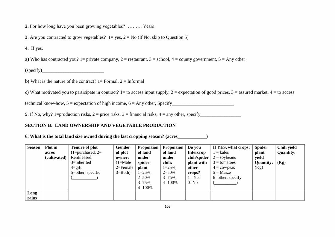
103
2. For how long have you been growing vegetables? ………. Years
3. Are you contracted to grow vegetables? 1= yes, 2 = No (If No, skip to Question 5)
4. If yes,
a) Who has contracted you? 1= private company, 2 = restaurant, 3 = school, 4 = county government, 5 = Any other
(specify)__________________________
b) What is the nature of the contract? 1= Formal, 2 = Informal
c) What motivated you to participate in contract? 1= to access input supply, 2 = expectation of good prices, 3 = assured market, 4 = to access
technical know-how, 5 = expectation of high income, 6 = Any other, Specify__________________________
5. If No, why? 1=production risks, 2 = price risks, 3 = financial risks, 4 = any other, specify_________________
SECTION B: LAND OWNERSHIP AND VEGETABLE PRODUCTION
6. What is the total land size owned during the last cropping season? (acres____________)
Season
Plot in
acres
(cultivated)
Tenure of plot
(1=purchased, 2=
Rent/leased,
3=inherited
4=gift
5=other, specific
(___________)
Gender
of plot
owner:
(1=Male
2=Female
3=Both)
Proportion
of land
under
spider
plant 1=25%,
2=50%
3=75%,
4=100%
Proportion
of land
under
chili:
1=25%,
2=50%
3=75%,
4=100%
Do you
Intercrop
chili/spider
plant with
other
crops?
1= Yes
0=No
If YES, what crops:
1 = kales
2 = soybeans
3 = tomatoes
4 = cowpeas
5 = Maize
6=other, specify
(__________)
Spider
plant
yield
Quantity:
(Kg)
Chili yield
Quantity:
(Kg)
Long
rains

104
Short
rains
INPUT USE
7. SEEDS
Crop Variety
grown:
0=local
1=improved
2=both
Quantity
of seeds
used (kg)
Mode of
acquisition:
1=bought
0= non-
bought
If bought where is
the source:
1=agro-vets
2=seed company
3=open air market
4=Neighbour/other
farmers
5=other, specify
Mode of
payment
for the
seed:
1=cash
2=credit
3=both
If non-bought:
1=Own saved
2=farmers to
farmers exchange
3=gift from
family/neighbor
4=Other, specify
If bought:
How much
did you
pay per
(Kg)
Constraints
faced in
accessing
seeds:
1= poor
availability
of seeds,
2=high
prices of
seed
3=presence
of
counterfeit
seeds
4=poor
quality seeds
5=other,
specify
Chili
Spider
plant
8. Did you use fertilizer during the last cropping season ? 1. Yes 0. No if NO skip to question 12
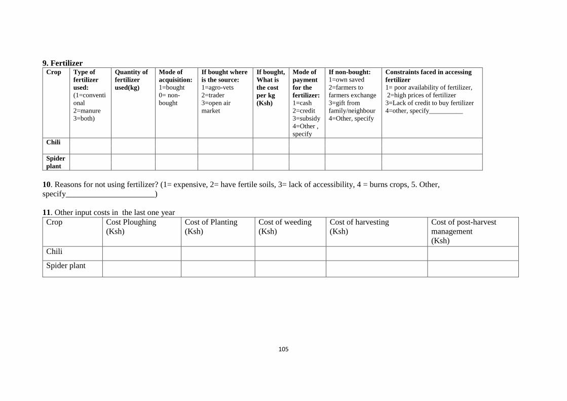
105
9. Fertilizer Crop Type of
fertilizer
used:
(1=conventi
onal
2=manure
3=both)
Quantity of
fertilizer
used(kg)
Mode of
acquisition:
1=bought
0= non-
bought
If bought where
is the source:
1=agro-vets
2=trader
3=open air
market
If bought,
What is
the cost
per kg
(Ksh)
Mode of
payment
for the
fertilizer:
1=cash
2=credit
3=subsidy
4=Other ,
specify
If non-bought:
1=own saved
2=farmers to
farmers exchange
3=gift from
family/neighbour
4=Other, specify
Constraints faced in accessing
fertilizer
1= poor availability of fertilizer,
2=high prices of fertilizer
3=Lack of credit to buy fertilizer
4=other, specify__________
Chili
Spider
plant
10. Reasons for not using fertilizer? (1= expensive, 2= have fertile soils, 3= lack of accessibility, 4 = burns crops, 5. Other,
specify______________________)
11. Other input costs in the last one year
Crop Cost Ploughing
(Ksh)
Cost of Planting
(Ksh)
Cost of weeding
(Ksh)
Cost of harvesting
(Ksh)
Cost of post-harvest
management
(Ksh)
Chili
Spider plant

106
12. Risks affecting vegetable production Risk factor Did you encounter this
risk factor in the last 5
planting seasons (1=yes,
0=No)
If yes how many
times did it occur in
the last 5 seasons
Did you put in place
any strategies to
prevent the risk factor
before it happens
(1=Yes, 0=No)
If YES What risk
adaptation strategy did
you put in place before
risk occurrence:
1=change crop varieties
2=early planting
3=crop diversification
4=Savings
5= change planting sites
6= increased seed rate
7=more of off-farm
employment
8=None
9=other, specify
What proportion of
vegetable yield did you lose
due to this risk factors
(1=25%, 2=50%, 3=75%,
4=100)
Drought
Too much rain/floods
Crop pests/diseases
Hail storms
Theft of assets/crops
Spoilage of crops

107
SECTION C
MARKETING
13. Did you sell vegetable after the last cropping season ? (1=Yes, 0=No) ____. Type of market
(MAIN)
Quantity of
vegetable
sold in
during last
season
Unit Price per
Unit
Period to
payment
after
selling,
weeks (zero
if
immediatel
y)
Do you have a contract
with the buyer
1= Yes
2=No
If YES what are the terms of
this contract:
1= Pay immediately
2= pay after some duration
3=advance of inputs + cash
4= Other, specify
(_________)
Transport
costs
Cess tax
Farm gate
Institutional
markets
(schools,
hospitals)
County
government
market
Brokers
/middlemen
Village market
Other, Specify

108
14. For contract farmers,
a). Who sets the price? 1=Buyer, 2=Seller, 3=Both agree________
b). How is produce delivery done? 1=Farmer delivers, 2=Buyer picks from the firm, 3=Group delivery, 4=Other, Specify______
c). What are the rules governing contracts? ________________________________________________________________________
d). What are the challenges experienced with contract farming? 1=Very high standards, 2=Low prices, 3=Violation of terms by the buyer,
4=low education, 5=lack of information, 6=Climate change, 7=Inadequate production resources, 8Other, specify___________
e). Are contracts effective? 1=Agree, 2=Strongly agree, 3=Disagree, 4=Strongly disagree, 5=Not sure_______
15. a) Did you get market information before you decided to sell the crop? (1=Yes, 0 = No)________
b) If yes, what was your MAIN source of information? (1= farmer coop/groups, 2=neighbor farmers, 3=seed traders/ agrovets, 4=research
centre,
5=extension provider, 6=radio/TV, 7=mobile phone, 8=other, specify)__________
16. Have you ever failed to sell vegetable due to lack of buyers? (1=Yes, 0=No)________
17. Have you ever failed to sell vegetable due to poor prices? (1=Yes, 0=No)___________
18. Distance to the nearest MAIN MARKET CENTRE from residence in (KM)_______
19. Average transport cost to and from the nearest main market per person_________

109
SECTION D: INSTITUTIONAL SUPPORT SERVICES
20. Social capital and credit access
Have you been a member of any development group since 2014? (1= Yes, 0= No) ____ if YES please fill the details in the table below: If NO
skip to Q.21 Type of group Member to
group(1=Yes,
0=No)
If yes duration of
membership
What is the most
(ONE) important
group function:
1=produce
marketing
2=input access
3=savings and
credit
4=farmer
trainings
5=transport
services
6.Agricultural
production
7=other,
specify
Role in the
group:
1=official
0=ordinary
member
Are you still a
member now:
1=Yes, 0=No
If NO, reasons for leaving
group:
1=group was not profitable
2=poor mgt and corrupt
officials
3=unable to pay annual
subscription fee
4=Group ceased to exit
5.=Other, specify
Women group
SACCO/credit
group
Farmer
coops/input supply
Producer and
marketing groups
Youth group
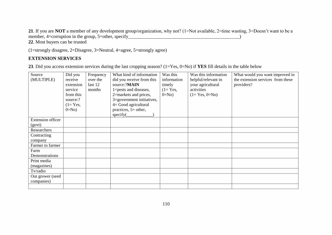
110
21. If you are NOT a member of any development group/organization, why not? (1=Not available, 2=time wasting, 3=Doesn’t want to be a
member, 4=corruption in the group, 5=other, specify_______________________________________________)
22. Most buyers can be trusted
(1=strongly disagree, 2=Disagree, 3=Neutral, 4=agree, 5=strongly agree)
EXTENSION SERVICES
23. Did you access extension services during the last cropping season? (1=Yes, 0=No) if YES fill details in the table below
Source
(MULTIPLE)
Did you
receive
extension
service
from this
source:?
(1= Yes,
0=No)
Frequency
over the
last 12
months
What kind of information
did you receive from this
source:?MAIN
1=pests and diseases,
2=markets and prices,
3=government initiatives,
4= Good agricultural
practices, 5= other,
specify(____________)
Was this
information
timely
(1= Yes,
0=No)
Was this information
helpful/relevant in
your agricultural
activities
(1= Yes, 0=No)
What would you want improved in
the extension services from these
providers?
Extension officer
(govt)
Researchers
Contracting
company
Farmer to farmer
Farm
Demonstrations
Print media
(magazines)
Tv/radio
Out grower (seed
companies)

111
24. Credit services
Have you ever applied for credit over the last two years? (1=Yes, 0=No)_________ IfNO skip to Q. 25 Source of Credit
MAIN
Did you
get it.
(1=Yes,
0=No)
If YES, how
was it
received?
1=as a group,
2=Individual
IF YES what
proportion
of the
credit
applied for
did you
get:
1=1/4,
2=1/2,
3=3/4,
4=all
Main use of credit:
1=farm inputs
2=school fees
3=food
4=land
5=livestock
6=offset a problem
one had
7=other,
specify_________
Did you
use ALL
of this
credit for
the
intended
purpose:?
1= Yes
0=No
If NO, how else did
you use this credit:
1=farm inputs
2=school fees
3=food
4=land
5=livestock
6=offset a problem one
had
7=Farm
implements/equipment
8=non -farm
business/trade
9=buy livestock
10=other,
specify_________
If NO, why did
you not get the
requested
amount(MAIN):
1=high default
rate
2=lacked
guarantors
3=didn’t adhere
to all
requirements
4=lacked
collateral
5=couldn’t access
lender
6=Age limit
7=don’t know
8=Other(specify)
Have
you
started
repaying
this
loan?
(1=Yes,
0=No)
If YES,
what
proportion
have you
repaid:
1=1/4,
2=1/2,
3=3/4,
4=all
Farmer
group/cooperative
Merry go Round
Bank
Sacco
Relative
Neighbour
Friends
Other (specify)

112
25. If you did not apply for credit what was the main reason? (1=high interests rate, 2=lacked collateral, 3=too much paper work, 4=borrowing
is risky, 5=expected to be rejected so I dint try it, 6=fear loans, 7= I don’t need it 8. Other. Specify_________________________)
SECTION E: VALUE-CHAIN GOVERNANCE
26. (a) To what extent do you agree with the following statement? (1=agree, 2=strongly agree, 3=disagree, 4=strongly disagree,5=Not sure)
Transaction complexity The contracting firms/buyers exchange considerable
information with us (e.g. product requirements)
The contracting firm/buyer require more than the
contractual agreement to award us business
Ability to codify Technology is the same across neighboring farms
We are well conversant with the contracting firm’s/buyers
technical standards
Supply base capabilities We are able to timely deliver complete products that meet
market requirements with minimum input from the
buyers.
The buyers do not spend more time monitoring us to fulfil
our commitments.

113
b) Vegetable Value chain management
Value-chain stage Who coordinates this stage?
1=Farmer
2=Farmer groups
3=Buyer/firm
4=Government
5=Other Specify
What rules apply in coordination of
this stage?
What are the challenges in
this stage?
Input supply
Production
Transportation
Value addition
Assembling
Marketing

114
SECTION F: LIVELIHOODS
27. Household Asset Ownership ASSET NAME DO YOU HAVE THIS ASSET
(1=Yes 0=No)
NUMBER CURRENTLY OWNED CURRENT VALUE (KSHS)
1.Ox-plough
2.Ox-cart
3.Radio
4. Television
5. Mobile phone
6. Wheelbarrow
7.Mortocycle
8. Pick-up
9.Machete
10.Hoe
11. Car/pickup
12Tractor
13Slasher
14Spraypump
15.Shovels
Income
28. (a) How much do you earn on-farm per cropping season?____________________________________________(Kshs)
AMOUNT(Ksh) Tick
500-1000
1001-1500
1501-2000
2001-3000
3001-5000
5001-7000
7001-10,000
10,001-20,000
20,001-30,000
Above 30,000

115
b) How much do you earn off-farm per cropping season? ____________________________________________(Kshs)
Savings
29. How much have you been saving from vegetable production per season on average? ______________________________(Kshs)
Amount Tick
0-1000
1001-1500
1501-2000
2001-3000
3001-5000
5001-7000
7001-10,000
10,001-20,000
20,001-30,000
Above 30,000
SECTION G: SOCIO-DEMOGRAPHICS
30. How many times has any of the household members sort medical attention in the last one month?_________
31. Education level of children
Child’s, Sex 1=Male, 0=Female Education level, 0=None , 1=Primary, 2=Secondary,
3=Tertiary

116
32.Respondent’s MAIN occupation? (1=farmer, 2=civil servant, 3=student, 4=teacher, 5=trader, 6=tailor, 7=boda boda, 8=casual laborer
(Juakali), 9=other, specify__________________)
33. Farmer’s age in years. __________
34. Farmer’s Sex , 1=Male, 0=Female
35. How many people live and depend on the household for food on a daily basis? __________
36. What is the total number of the household members_____________?
37. Number of years of formal schooling for respondent _____________
THANK YOU FOR YOUR TIME

117
Appendix 2: VIF for probit model
Variable VIF 1/VIF
Distance to market 1.06 0.939
Farming experience 1.12 0.890
Age of the farmer 1.53 0.652
Land size 1.2 0.831
Household size 1.23 0.810
Gender 1.25 0.800
Membership to group 1.45 0.691
Access to extension services 1.34 0.744
Access to credit 1.26 0.791
Household type 1.28 0.779
County 1.11 0.899
Off-farm income 1.08 0.928
Mean VIF 1.24
Appendix 3: VIF for OLS
Variable VIF 1/VIF
Farming experience 1.11 0.904
Age 1.55 0.645
Land size 1.21 0.828
Household size 1.24 0.809
Gender 1.26 0.795
Membership to group 1.43 0.699
Access to extension services 1.35 0.740
Access to credit 1.27 0.789
Household type 1.4 0.715
Gender of plot owner 1.17 0.852
County 1.12 0.895
Income 1.08 0.927
Mean VIF 1.26

118
Appendix 4: Partial and Semi-partial correlations for income with
independent variables
Appendix 5: Stochastic frontier instruction file
Code Interpretation
1 1 = Error components model, 2 = TE effects model
lww-dta.txt data file name
lww-out.txt output file name
1 1 = production function, 2 = cost function
y logged dependent variable (y/n)
(173,127) number of cross sections
1 number of time periods
(173, 127) number of observations in total
4 number of regressor variables (Xs)
y/n mu (y/n) [or delta0 (y/n) if using TE effects model]
y/n delta (y/n) [or number of TE effects regressors (Zs)]
n starting values specified (y/n)
Appendix 6: Spider plants and chili Shazam codes
CHILI
*1. READ DATA AND ESTIMATED PARAMETERS OF GROUP STOCHASTIC
FRONTIERS
sample 1 254
genr one = 1
dim group 254 t 254 y 254 famlab 254 hirlab 254 Lnseed 254 Lnplot 254
Variable
Partial
Correlation
Semi-partial
Correlation Partial
Semi-
partial Significance
Variable Corr. Corr. Corr.^2 Corr.^2 Value
A3_CONTRA~D 0.498 0.484 0.248 0.234 0.000
lnpoolmkt~t 0.059 0.050 0.004 0.003 0.318
lnpoolland 0.056 0.047 0.003 0.002 0.343
lnpoolage -0.088 -0.074 0.008 0.006 0.135
lnpoolHHs~e 0.061 0.052 0.004 0.003 0.299
lnpoolexp 0.088 0.074 0.008 0.006 0.137
lnpoolsch~l 0.032 0.027 0.001 0.001 0.582
D20_DEV_G~P 0.027 0.023 0.001 0.001 0.644
D23_EXTEN~S 0.005 0.004 0.000 0.000 0.930
D24_CREDIT -0.046 -0.039 0.002 0.002 0.434

119
read (hhp.txt) group t y famlab hirlab Lnseed Lnplot/ beg=1 end=70 list
read (hhn.txt) group t y famlab hirlab Lnseed Lnplot/ beg=71 end=127 list
read (hht.txt) group t y famlab hirlab Lnseed Lnplot/ beg=128 end=254 list
sample 1 254
print group t y famlab hirlab Lnseed Lnplot
matrix x = one|famlab|hirlab|Lnseed|Lnplot
print x
dim x1 70 5 x2 57 5 x3 127 5
copy x x1 / frows = 1;70 trows = 1;70
copy x x2 / frows = 71;127 trows = 1;57
copy x x3 / frows = 128;254 trows = 1;154
dim fem 5 mal 5 joi 5
read (phhh.txt) fem mal joi / beg=1 end=5 list
matrix s = fem|mal|joi
print s
sample 1 5
dim s1 5 s2 5 s3 5
copy s s1 / fcols = 1;1 tcols = 1;1
copy s s2 / fcols = 2;2 tcols = 1;1
copy s s3 / fcols = 3;3 tcols = 1;1
*2. CONSTRUCT DATA MATRICES AND ESTIMATE METAFRONTIER
matrix g1 = x1*s1
matrix g2 = x2*s2
matrix g3 = x3*s3
print g1
print g2
print g3
matrix b = -(g1'|g2'|g3')'
print b
stat x / means = xbar
matrix c = (-xbar'|xbar')'
matrix A = (-x|x)
print A
print C
?lp c A b /iter = 6000 primal = bstar
print bstar
*3. USE METAFRONTIER ESTIMATES TO OBTAIN TECHNOLOGY GAP RATIOS
dim meta 5
read (pppc.txt) meta / beg=1 end=5 list
sample 1 5
matrix starb = meta
print starb
matrix g1star = x1*starb
matrix g2star = x2*starb
matrix g3star = x3*starb

120
print g1star
print g2star
print g3star
matrix dev1 = g1star-g1
matrix dev2 = g2star-g2
matrix dev3 = g3star-g3
print dev1
print dev2
print dev3
matrix tgr1 = exp(g1)/exp(g1star)
matrix tgr2 = exp(g2)/exp(g2star)
matrix tgr3 = exp(g3)/exp(g3star)
sample 1 70
stat tgr1
print group tgr1
sample 1 57
print group tgr2
stat tgr2
sample 1 127
print group tgr3
stat tgr3
SPIDER
*1. READ DATA AND ESTIMATED PARAMETERS OF GROUP STOCHASTIC
FRONTIERS
sample 1 346
genr one = 1
dim group 346 t 346 y 346 famlab 346 hirlab 346 Lnseed 346 Lnplot 346
read (spt.txt) group t y famlab hirlab Lnseed Lnplot/ beg=1 end=79 list
read (snc.txt) group t y famlab hirlab Lnseed Lnplot/ beg=80 end=173 list
read (spo.txt) group t y famlab hirlab Lnseed Lnplot/ beg=174 end=346 list
sample 1 346
print group t y famlab hirlab Lnseed Lnplot
matrix x = one|famlab|hirlab|Lnseed|Lnplot
print x
dim x1 79 5 x2 94 5 x3 173 5
copy x x1 / frows = 1;79 trows = 1;79
copy x x2 / frows = 80;173 trows = 1;94
copy x x3 / frows = 174;346 trows = 1;173
dim fem 5 mal 5 joi 5
read (tpspi.txt) fem mal joi / beg=1 end=5 list
matrix s = fem|mal|joi
print s
sample 1 5
dim s1 5 s2 5 s3 5

121
copy s s1 / fcols = 1;1 tcols = 1;1
copy s s2 / fcols = 2;2 tcols = 1;1
copy s s3 / fcols = 3;3 tcols = 1;1
*2. CONSTRUCT DATA MATRICES AND ESTIMATE METAFRONTIER
matrix g1 = x1*s1
matrix g2 = x2*s2
matrix g3 = x3*s3
print g1
print g2
print g3
matrix b = -(g1'|g2'|g3')'
print b
stat x / means = xbar
matrix c = (-xbar'|xbar')'
matrix A = (-x|x)
print A
print C
?lp c A b /iter = 6000 primal = bstar
print bstar
*3. USE METAFRONTIER ESTIMATES TO OBTAIN TECHNOLOGY GAP RATIOS
dim meta 5
read (tspmeta.txt) meta / beg=1 end=5 list
sample 1 5
matrix starb = meta
print starb
matrix g1star = x1*starb
matrix g2star = x2*starb
matrix g3star = x3*starb
print g1star
print g2star
print g3star
matrix dev1 = g1star-g1
matrix dev2 = g2star-g2
matrix dev3 = g3star-g3
print dev1
print dev2
print dev3
matrix tgr1 = exp(g1)/exp(g1star)
matrix tgr2 = exp(g2)/exp(g2star)
matrix tgr3 = exp(g3)/exp(g3star)
sample 1 79
stat tgr1
print group tgr1
sample 1 94
print group tgr2
stat tgr2
sample 1 173 print group tgr3