Partial Di¤erential Equations Notes

Professor: Jalal Shatah Eduardo Corona

Spring 2009

Contents

I Introduction 1

1 1st order PDEs: The Method of Characteristics 21.1 Linear PDE . . . . . . . . . . . . . . . . . . . . . . . . . . . . . . . . . . . . . . . . . . . . . . 21.2 Nonlinear 1st order PDEs . . . . . . . . . . . . . . . . . . . . . . . . . . . . . . . . . . . . . . 3

1.2.1 What are conservation laws? . . . . . . . . . . . . . . . . . . . . . . . . . . . . . . . . 41.3 Generalization to higher dimensions . . . . . . . . . . . . . . . . . . . . . . . . . . . . . . . . 6

1.3.1 Power Series . . . . . . . . . . . . . . . . . . . . . . . . . . . . . . . . . . . . . . . . . 71.4 Weak Solutions: Shock waves and jump conditions . . . . . . . . . . . . . . . . . . . . . . . . 7

1.4.1 What is a weak solution? . . . . . . . . . . . . . . . . . . . . . . . . . . . . . . . . . . 71.4.2 The Rankin-Huguenot jump condition . . . . . . . . . . . . . . . . . . . . . . . . . . . 81.4.3 Are weak solutions unique? . . . . . . . . . . . . . . . . . . . . . . . . . . . . . . . . . 91.4.4 Which weak solution to pick? . . . . . . . . . . . . . . . . . . . . . . . . . . . . . . . 11

1.5 Nonlinear Equations: Cauchy Kovalewski . . . . . . . . . . . . . . . . . . . . . . . . . . . . . 111.5.1 Shatah�s summary: Characteristics & the C-K Theorem . . . . . . . . . . . . . . . . . 121.5.2 Characteristics as the "Carriers of Discontinuity" . . . . . . . . . . . . . . . . . . . . . 13

2 Classi�cation of 2nd order linear PDEs (Hadamard) 13

3 Hyperbolic Equations 143.1 Homogeneous equation . . . . . . . . . . . . . . . . . . . . . . . . . . . . . . . . . . . . . . . . 143.2 Nonhomogeneous equations . . . . . . . . . . . . . . . . . . . . . . . . . . . . . . . . . . . . . 153.3 Next level of complication: extra terms . . . . . . . . . . . . . . . . . . . . . . . . . . . . . . . 16

3.3.1 The Newton Method . . . . . . . . . . . . . . . . . . . . . . . . . . . . . . . . . . . . . 163.4 Hyperbolic systems . . . . . . . . . . . . . . . . . . . . . . . . . . . . . . . . . . . . . . . . . . 17

3.4.1 Newton Method (revisited) . . . . . . . . . . . . . . . . . . . . . . . . . . . . . . . . . 17

II Background Material 183.5 Fourier Transforms . . . . . . . . . . . . . . . . . . . . . . . . . . . . . . . . . . . . . . . . . . 183.6 Sobolev Spaces Hk() . . . . . . . . . . . . . . . . . . . . . . . . . . . . . . . . . . . . . . . . 193.7 Distributions . . . . . . . . . . . . . . . . . . . . . . . . . . . . . . . . . . . . . . . . . . . . . 20

3.7.1 Weak derivative and other operations on D� . . . . . . . . . . . . . . . . . . . . . . . 21

1

Part I

Introduction1 1st order PDEs: The Method of Characteristics

Lecture 1 (15/01/09)

1.1 Linear PDE

We can start by thinking of a set of particles moving in 1D, their motion given by the equation:

_x = v(x; t)

Additionally, there might be a quantity, or "piece of information" that is carried by these particles and thatwe are interested in measuring (e.g. charge, mass, velocity, etc), denoted by u. If this information is notchanging with time, then we have the following:

0 = Dtu =d

dtu( (t)) =

du

dt+ v

du

dx

This is a typical advection equation.We can now consider the inverse process: we have a function u such that it satis�es the advection equation:�

ut + vux = 0u(x; 0) = f(x)

�For each point x0 2 R, we can then solve the ODE to obtain x = (t; x0):�

_x = v(x; t)x(0) = x0

�By our hypothesis, Dtu = 0; and so:

u(x; t) = f(x0)

x0 = �1(t; x)

u(x; t) = f( �1(t; x))

Example 1 We want to solve �ut + ux = 0u(0; x) = sinx

�v � 1, and the solution to the ODE _x � 1 with x(0) = x0 is x = t+ x0. Hence,

x0 = x� t

u(x; t) = sin(x� t)

This is basically telling us that the sine wave is being transported with speed 1.

Example 2 Modifying the previous equation, we are now interested in:�ut + ux = uu(0; x) = f(x)

�Again, the trajectory is given by x = x0 + t, but Dtu = u. So,

u(x; t) = f(x� t)et

2

Example 3 Now, we try to solve a general linear 1st order PDE using this method:

a(x; y)ux + b(x; y)uy = c(x; y)

We could assume a 6= 0 and/or b 6= 0 and solve it like the previous examples. However, it is best to solve anODE directly. For that matter, we introduce a new parameter � :�

dxd� = a(x; y) , dy

d� = b(x; y)(x; y)j�=0 = (x0; y0)

�By solving this ODE, I get a curve (x; y) = (�; �)(�); and the equation simpli�es to:

D�u = c(�; �)

Hence, an integration formula yields:

u = u0 +

Z �

0

c(�(�); �(�))d�

The last step involves solving for (x0; y0) and plugging them in.

1.2 Nonlinear 1st order PDEs

We now proceed to the next level of complication: a semilinear 1st order PDE. That is,

a(x; y; u)ux + b(x; y; u)uy = c(x; y; u)

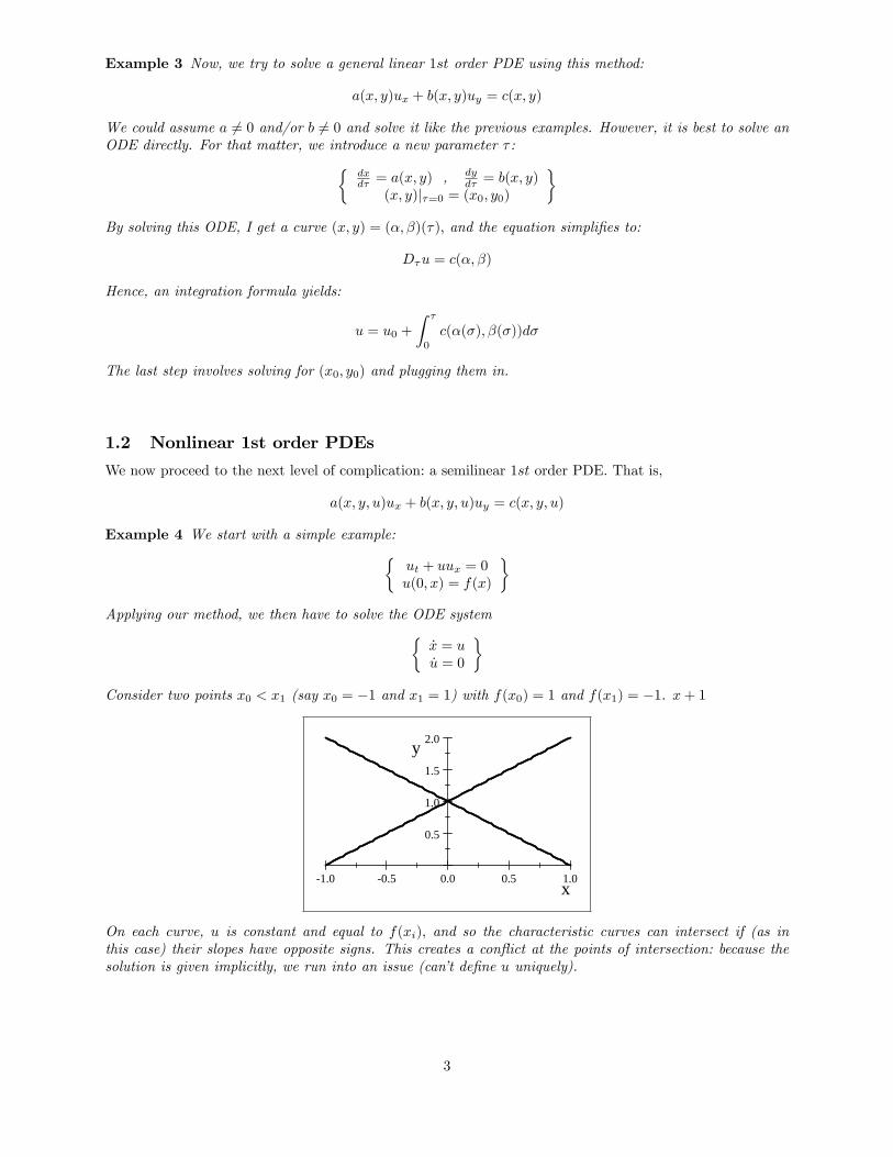
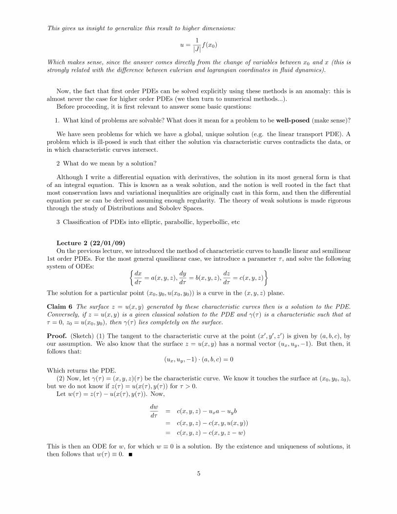
Example 4 We start with a simple example:�ut + uux = 0u(0; x) = f(x)

�Applying our method, we then have to solve the ODE system�

_x = u_u = 0

�Consider two points x0 < x1 (say x0 = �1 and x1 = 1) with f(x0) = 1 and f(x1) = �1. x+ 1

­1.0 ­0.5 0.0 0.5 1.0

0.5

1.0

1.5

2.0

x

y

On each curve, u is constant and equal to f(xi); and so the characteristic curves can intersect if (as inthis case) their slopes have opposite signs. This creates a con�ict at the points of intersection: because thesolution is given implicitly, we run into an issue (can�t de�ne u uniquely).

3

This example makes us think about the problem we have been posing: we want to obtain a global solutionfrom local data. In the case where characteristic curves intersect, it is clear that the solution exists only fora little bit of time, at best.Now, if we blindly solve for the system, we get:

x = ut+ x0

u = f(x� ut)

From this implicit equation, we must solve for u. Let g(x; t;u) = u � f(x � ut). By the Implicit FunctionTheorem, in order to be able to solve for u (locally), we require:

gu = 1 + tf0(x� ut) 6= 0

So, for instance if f 0 > 0 or t is small, a solution always exists.This equation we have just studied is important, since it is a prototype for conservation laws.

1.2.1 What are conservation laws?

Let �(x; t) describe the family of characteristic curves, q a quantity that is conserved over time (mass, charge,momentum, energy, etc), given by a density u(x; t):

q(t) =

Z �(x1;t)

�(x0;t)

u(x; t)dx

Now, we take a derivative with respect to time, and let _� = v (velocity):

0 =

Z �(x1;t)

�(x0;t)

ut(x; t)dx+ vuj�(x1;t)�(x0;t)

Since x0 and x1 are arbitrary, this implies: �ut + (vu)x = 0u(x; 0) = f(x)

�Sometimes v depends on u (quasilinear case) or is given (linear case).

Case 5 If v is given, we have:ut + vux = �vxu

The ODE is _x = v; and once we solve it, we plug into Dtu = �vxu, which is separable:

ln(u) = �Zvx(x; t)dt

u(x; t) = exp

��Zvx(x; t)dt

�f(x0(x; t))

We can rewrite the solution to this equation in an interesting way. The solution to our system is given onthe curves x(t; x0): But then, di¤erentiating _x = v yields:� d _x

dx0= vx(x; t)

dxdx0

d _xdx0(0) = 1

�And so,

dx

dx0= exp

�Zvx(x; t)dt

�So,

u =1dxdx0

f(x0)

4

This gives us insight to generalize this result to higher dimensions:

u =1

jJ jf(x0)

Which makes sense, since the answer comes directly from the change of variables between x0 and x (this isstrongly related with the di¤erence between eulerian and lagrangian coordinates in �uid dynamics).

Now, the fact that �rst order PDEs can be solved explicitly using these methods is an anomaly: this isalmost never the case for higher order PDEs (we then turn to numerical methods...).Before proceeding, it is �rst relevant to answer some basic questions:

1. What kind of problems are solvable? What does it mean for a problem to be well-posed (make sense)?

We have seen problems for which we have a global, unique solution (e.g. the linear transport PDE). Aproblem which is ill-posed is such that either the solution via characteristic curves contradicts the data, orin which characteristic curves intersect.

2 What do we mean by a solution?

Although I write a di¤erential equation with derivatives, the solution in its most general form is thatof an integral equation. This is known as a weak solution, and the notion is well rooted in the fact thatmost conservation laws and variational inequalities are originally cast in this form, and then the di¤erentialequation per se can be derived assuming enough regularity. The theory of weak solutions is made rigorousthrough the study of Distributions and Sobolev Spaces.

3 Classi�cation of PDEs into elliptic, parabollic, hyperbollic, etc

Lecture 2 (22/01/09)On the previous lecture, we introduced the method of characteristic curves to handle linear and semilinear

1st order PDEs. For the most general quasilinear case, we introduce a parameter � ; and solve the followingsystem of ODEs: �

dx

d�= a(x; y; z);

dy

d�= b(x; y; z);

dz

d�= c(x; y; z)

�The solution for a particular point (x0; y0; u(x0; y0)) is a curve in the (x; y; z) plane.

Claim 6 The surface z = u(x; y) generated by these characteristic curves then is a solution to the PDE.Conversely, if z = u(x; y) is a given classical solution to the PDE and (�) is a characteristic such that at� = 0; z0 = u(x0; y0), then (�) lies completely on the surface.

Proof. (Sketch) (1) The tangent to the characteristic curve at the point (x0; y0; z0) is given by (a; b; c); byour assumption. We also know that the surface z = u(x; y) has a normal vector (ux; uy;�1). But then, itfollows that:

(ux; uy;�1) � (a; b; c) = 0Which returns the PDE.(2) Now, let (�) = (x; y; z)(�) be the characteristic curve. We know it touches the surface at (x0; y0; z0);

but we do not know if z(�) = u(x(�); y(�)) for � > 0.Let w(�) = z(�)� u(x(�); y(�)). Now,

dw

d�= c(x; y; z)� uxa� uyb

= c(x; y; z)� c(x; y; u(x; y))= c(x; y; z)� c(x; y; z � w)

This is then an ODE for w; for which w � 0 is a solution. By the existence and uniqueness of solutions, itthen follows that w(�) � 0.

5

Now, when can I construct a solution of the PDE from the ODE? We can deduce this from the conditionsfor the Implicit Function Theorem: we originally have the surface (x; y; z)(� ; s); and I want to write it asz = u(x; y). This is possible if and only if:

det

�x� y�xs ys

�6= 0

I can compute this at the initial point, with (x; y) = (f(s); g(s)); z = h(s) = u(x; y):

det

�a bfs gs

�6= 0

This essentially says the vectors (a; b) and (fs; gs) cannot be parallel. In other words, the PDE is solvableby this method (locally) if and only if the characteristic curves "take o¤" from the curve ofinitial values. In other words, we may not impose initial data on a curve that is characteristic (or with atangent vector which is parallel to a characteristic at some point).

Theorem 7 Given a quasilinear equation aux+buy = c (with a; b; c su¢ ciently smooth), C = (f; g)(s) 2 C1and "Cauchy data" ujC = h(s); then there exists a unique solution in a neighborhood of C provided the "non-characteristic" condition holds.

det

�a bfs gs

�6= 0

Example 8 For ut + uux = 0; ujt=0 = h(x), the curve ft = 0g is never characteristic, since dtds � 1.

Example 9 u � 1; for 0 � x � 1. This is also solvable, but we can only tell what u is in the region sweptby the characteristics f(x; y) : x� 1 � y � xg.

1.3 Generalization to higher dimensions

For x 2 Rd we have the following quasilinear PDE (where A and C are su¢ ciently smooth):

A(x; u)>ru = C(x; u)

We can then obtain the d+ 1 dimensional ODE system:�dx

d�= A;

dz

d�= C

�As before, we solve this from an initial point (x0; u(x0)); and call it a characteristic curve. Everything followsverbatim, except now the non-degeneracy / non-characteristic condition is more complicated.A Cauchy problem now consists of providing initial data on a d� 1 dimensional hypersurface, which can

be either written as X(0; y1; ::; yd�1) (determined by d� 1 parameters) with nonzero Jacobian or as a levelset '(x) = 0 with r' 6= 0.We then solve the ODE on each point of this surface S, obtaining fX(� ; y); Z(� ; y)g. Although the IFT

again yields a condition (the Jacobian being nonzero), but it is usually very burdensome to check.

Instead, in the case where the surface is given by a level set, it is better to usea change of variables(�1; ::; �d) = (x; '(x)): So,

A>ru =Xi;k

Ai@u

@�k

@�k@xi

Then our hypersurface becomes �d = 0, and the non-degeneracy condition now reads:Xi

Ai@'

@xi6= 0

Since the normal to the hypersurface is r'; this is a straightforward extension of the non-characteristiccondition in 1D: characteristics must have a non-trivial normal component to the surface S.

6

1.3.1 Power Series

The �rst time you see an ODE, what do you try to do? We can either integrate, or try to come up with apower series solution. Lets try this for PDEs:

Example 10 Lets solve (again) ut + ux = 0 with u(0; x) = sin(x). We �rst write u(x; t) =P1

n=0 gn(x)tn

n! ;and from the PDE and initial conditions:

utjt=0 = �uxjt=0 = � cos(x)

Di¤erentiating once on time, we then have utt(0) = �uxt(0) = � sin(x), and we can continue this process.Thus,

u(x; t) = sin(x) + (�1) cos(x)t+ (�1)2

2[� sin(x)]t2 + (�1)

3

6[� cos(x)]t3 + :::

= sin(x� t)

Example 11 Now, we consider initial data u(s;�s) = sin(s). Now, I need to �nd ur; urr on the (r; s) plane(rotating 45�), so the coe¢ cient on the ODE must not vanish! Writing r = x� y and s = x+ y, we see thatthe coe¢ cient vanishes for ux � uy = 0.

Example 12 Lets consider the second order equation utt�uxx = 0 (wave equation). Then, after the changeof variables,

u(s; ') = u''('2t � '2x) + ::: = 0

And we need to determine u'' from the lower order terms. It is then clear that the non-characteristiccondition reads:

'2t � '2x = 0

j'tj = j'xj

And the characteristic curves are lines with slopes �1.

From this last example, we can glean that the "simbol" of the highest order terms in our PDE gives outthe non-characteristic condition, by replacing u with ', and the order as an exponent. For example, for theequation auxx + buxy + cuyy = 0 it would be the quadratic a'2x + b'x'y + c'

2y.

Lecture 3 (27/01/09)

1.4 Weak Solutions: Shock waves and jump conditions

1.4.1 What is a weak solution?

Lets recall one of our �rst examples for quasilinear equations. This example is especially relevant, since itcomes from a conservation law in �uid dynamics. It goes by the name of the inviscid Burgers equation, andis often applied to the modeling of gas dynamics and tra¢ c �ow. It is also a prototypical example of anequation for which the solution can develop discontinuities (shock waves):�

ut + uux = 0u(x; 0) = f(x)

�For this equation, we had obtained an implicit solution of the form u(x; t) = f(x� ut), and concluded thatit was necessary to have 1 + tf 0(x� �t) 6= 0 for t � 0. Hence, if f 0(x� �t) is negative, then this will vanishat t = 1=f 0.The key point here is to realize that, since this models the behavior of a physical phenomena,

there IS a solution. Hence, there must be a problem with the way we are seeking solutions.We then have to go back to the integral form of the conservation law, and �nd out what we mean by a

weak solution for this equation. The general form of a conservation law is the following: the change in time

7

of a quantity (mass, charge, momentum, etc) for which we have a density function u(x; t) is due to the �uxof that quantity on the boundary (in 1D; given by a �ux function F evaluated on a and x). That is:

d

dt

Z x

a

u(y; t)dy = F (u(x; t))� F (u(a; t))

Equivalently, we can write the following equation using a test function v 2 D(R2):Z 1

0

Z 1

�1uvt � F (u)vxdxdt = 0

The equivalence of these two can be shown by the use of test functions of the form v = �1(x) �2(t), where�1 is a smoothed �[a;x] and �2 a smoothed �[�;t], for a and � arbitrary.If u is regular, we can then push the di¤erential sign in / use integration by parts respectively and obtain

the PDE:ut � F 0(u)ux = 0

So, for our problem we have F (u) = �u2=2.

1.4.2 The Rankin-Huguenot jump condition

Now, what happens if u is not di¤erentiable? For instance, lets consider the case where u(x; t) is piecewisesmooth, with a jump discontinuity on the curve x = s(t). We will show in a moment that, in that event, uis a weak solution if it satis�es the PDE whenever it is C1, and if it jumps, it only does so on curves whichsatisfy the Rankin-Huguenot jump condition:

ds

dt=F (u+)� F (u�)

u+ � u�

Where u+(x0) and u�(x0) are the limits when x! x0 from each side of x = s(t).

Claim 13 If u is a weak solution as de�ned by the conditions above, then it satis�es the integral form of thecorresponding conservation law.

Proof. Clearly, in regions which do not include discontinuities, the PDE implies the integral equation andthere is nothing to show. Let be a ball centered around a point in (s(t); t), + the fraction on the rightside, and � on the left. Then, for ' 2 D()

0 =

Z 1

0

Z 1

�1u't � F (u)'xdxdt

=

Z+

u't � F (u)'xdxdt+Z�

u't � F (u)'xdxdt

Now, integrating by parts on each region:Z+

u't � F (u)'xdxdt = �Z+

[ut � F (u)ux]'dxdt+ZC

u�t � F (u)�x

=

ZC

u+�t � F (u+)�xdl

Since [ut � F (u)ux] vanishes a.e. on + (u is C1 and the integral equation here is equivalent to the PDE).On � we have the same situation, with �� = ��+ (normal vectors are opposite). Hence,Z

+

u't � F (u)'xdxdt+Z�

u't � F (u)'xdxdt

=

ZC

[u+ � u�]�t � [F (u+)� F (u�)]�xdl

8

Since this holds for all test functions, it implies that:

[u+ � u�]�t � [F (u+)� F (u�)]�x = 0

Now, for a curve given by x = s(t), the tangent vector is given by � = ( _s; 1); and so the normal vector is(�x; �t) = (�1; _s). Hence,

[u+ � u�] _s = [F (u+)� F (u�)]

Which returns the stipulated jump condition.

Remark 14 We can treat a generalization of this result using an identical process as the one shown above.We now want to apply the same procedure to the equation:

S0(u)ut � F 0(u)ux = 0

And moreover, we want to study the discontinuity on a curve given by (x(�); t(�)). In an analogue fashion,a weak solution for this equation is de�ned as u such that, for all ' 2 D(R2),

0 =

Z 1

0

Z 1

�1S(u)'t � F (u)'xdxdt

Following the same procedure, we conclude that:

[S(u+)� S(u�)]�t � [F (u+)� F (u�)]�x = 0

Now � = ( _x; _t); and � = (� _t; _x) and so:

[S(u+)� S(u�)] _x� [F (u+)� F (u�)] _t = 0

(or more generally, we need [S(u+)�S(u�)]dx� [F (u+)�F (u�)]dt to be an exact di¤erential). In the casethe curve is given by x = s(t); this reduces to:

ds

dt=F (u+)� F (u�)S(u+)� S(u�)

and our previous example corresponds to S(u) = u.

1.4.3 Are weak solutions unique?

Through several examples using the Burgers equation, we will see that even if we go back to the conservationlaw and come up with weak solutions, these might not be unique. We will study a way to determine a uniquesolution (known as the viscosity solution) which is more signi�cant from a physical / modelling standpoint,and we will also see di¤erent phenomena such as shocks or rarefaction waves appear.

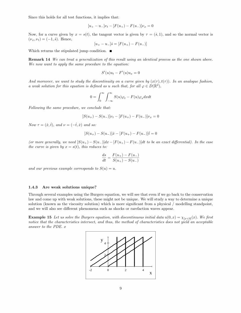
Example 15 Let us solve the Burgers equation, with discontinuous initial data u(0; x) = �[x<0](x): We �rstnotice that the characteristics intersect, and thus, the method of characteristics does not yield an acceptableanswer to the PDE. x

­2 0 2 4

2

4

x

y

9

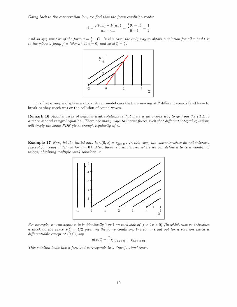
Going back to the conservation law, we �nd that the jump condition reads:

_s =F (u+)� F (u�)

u+ � u�=

12 (0� 1)0� 1 =

1

2

And so s(t) must be of the form x = t2 +C. In this case, the only way to obtain a solution for all x and t is

to introduce a jump / a "shock" at x = 0, and so s(t) = t2 .

­2 0 2 4

2

4

x

y

This �rst example displays a shock: it can model cars that are moving at 2 di¤erent speeds (and have tobreak as they catch up) or the collision of sound waves.

Remark 16 Another issue of de�ning weak solutions is that there is no unique way to go from the PDE toa more general integral equation. There are many ways to invent �uxes such that di¤erent integral equationswill imply the same PDE given enough regularity of u.

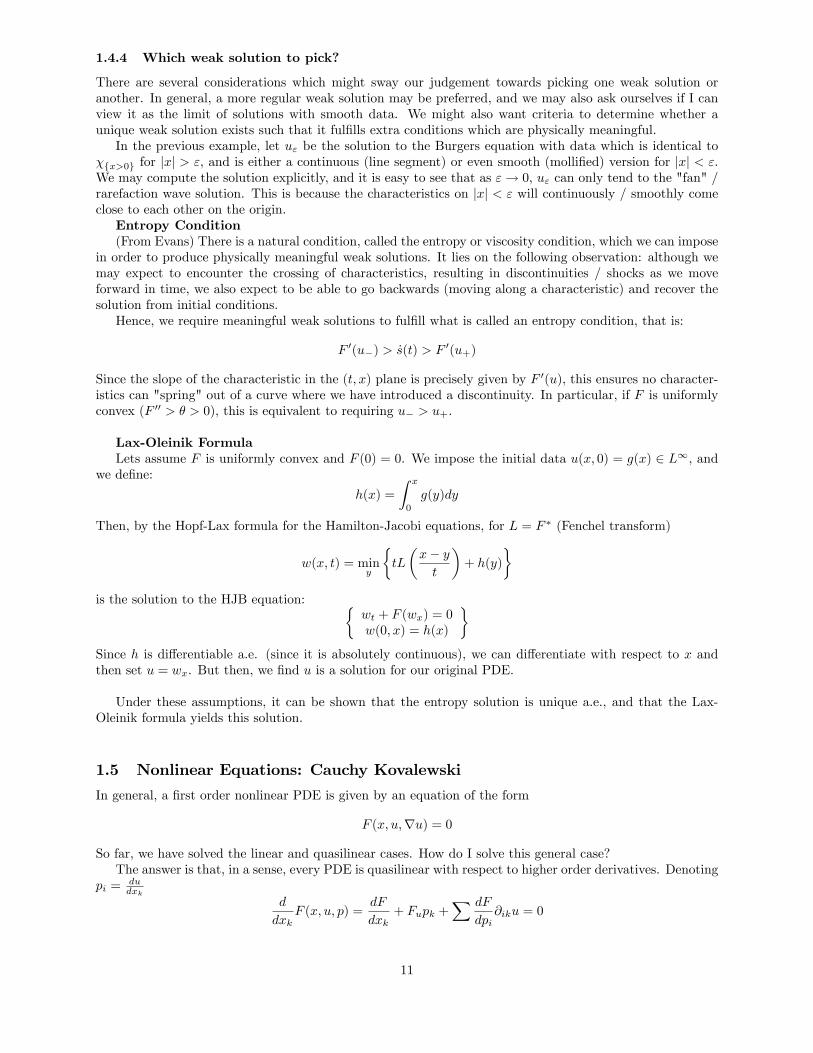
Example 17 Now, let the initial data be u(0; x) = �[x>0]. In this case, the characteristics do not intersect(except for being unde�ned for x = 0). Also, there is a whole area where we can de�ne u to be a number ofthings, obtaining multiple weak solutions. x

­1 0 1 2 3 4 5

1

2

3

4

5

x

y

For example, we can de�ne x to be identically 0 or 1 on each side of ft > 2x > 0g (in which case we introducea shock on the curve s(t) = t=2 given by the jump condition),We can instead opt for a solution which isdi¤erentiable except at (0; 0); say

u(x; t) =x

t�f0<x<tg + �fx>t>0g

This solution looks like a fan, and corresponds to a "rarefaction" wave.

10

1.4.4 Which weak solution to pick?

There are several considerations which might sway our judgement towards picking one weak solution oranother. In general, a more regular weak solution may be preferred, and we may also ask ourselves if I canview it as the limit of solutions with smooth data. We might also want criteria to determine whether aunique weak solution exists such that it ful�lls extra conditions which are physically meaningful.In the previous example, let u" be the solution to the Burgers equation with data which is identical to

�fx>0g for jxj > ", and is either a continuous (line segment) or even smooth (molli�ed) version for jxj < ".We may compute the solution explicitly, and it is easy to see that as "! 0; u" can only tend to the "fan" /rarefaction wave solution. This is because the characteristics on jxj < " will continuously / smoothly comeclose to each other on the origin.Entropy Condition(From Evans) There is a natural condition, called the entropy or viscosity condition, which we can impose

in order to produce physically meaningful weak solutions. It lies on the following observation: although wemay expect to encounter the crossing of characteristics, resulting in discontinuities / shocks as we moveforward in time, we also expect to be able to go backwards (moving along a characteristic) and recover thesolution from initial conditions.Hence, we require meaningful weak solutions to ful�ll what is called an entropy condition, that is:

F 0(u�) > _s(t) > F 0(u+)

Since the slope of the characteristic in the (t; x) plane is precisely given by F 0(u), this ensures no character-istics can "spring" out of a curve where we have introduced a discontinuity. In particular, if F is uniformlyconvex (F 00 > � > 0), this is equivalent to requiring u� > u+.

Lax-Oleinik FormulaLets assume F is uniformly convex and F (0) = 0. We impose the initial data u(x; 0) = g(x) 2 L1, and

we de�ne:

h(x) =

Z x

0

g(y)dy

Then, by the Hopf-Lax formula for the Hamilton-Jacobi equations, for L = F � (Fenchel transform)

w(x; t) = miny

�tL

�x� yt

�+ h(y)

�is the solution to the HJB equation: �

wt + F (wx) = 0w(0; x) = h(x)

�Since h is di¤erentiable a.e. (since it is absolutely continuous), we can di¤erentiate with respect to x andthen set u = wx. But then, we �nd u is a solution for our original PDE.

Under these assumptions, it can be shown that the entropy solution is unique a.e., and that the Lax-Oleinik formula yields this solution.

1.5 Nonlinear Equations: Cauchy Kovalewski

In general, a �rst order nonlinear PDE is given by an equation of the form

F (x; u;ru) = 0

So far, we have solved the linear and quasilinear cases. How do I solve this general case?The answer is that, in a sense, every PDE is quasilinear with respect to higher order derivatives. Denoting

pi =dudxk

d

dxkF (x; u; p) =

dF

dxk+ Fupk +

X dF

dpi@iku = 0

11

Then, we have the characteristic curves are given by solving the system:8<:dxid� =

dFdpi,dud� =

Pk pk

dxkd�

dpkd� = �

dFdxk

� FupkF (x; u; p) = 0

9=;(Insert example / from homework)From our previous results, we know the solution by the method of characteristics can�t always be computed

or doesn�t always make sense. The Cauchy Kovalewski theorem tells me how to solve the equation wt =F (t; x; w;rw) in the case where F is analytic, and we have an initial condition w(x; 0) = f(x) which isanalytic as well. In this case, it concludes that there exists a local solution in a neighborhood of (0; x0).The method used on this theorem is a power series expansion. The question it asks is, given that I have

this information, can I complete higher order derivatives? The key is that coe¢ cients can be majorized, andso we can compute the power series around a point.Generalizations: �rst, we can then apply this to the equation:

@mt w = G(t; x; w; @tw; ::; @m�1t w;D�w), j�j � m;�1 < m

With m � 1 pieces of information as initial data (Cauchy data), w(x; 0) = f0; ::; wm�1(x; 0) = fm�1. I can

then change this into an instance of the �rst case, so that the original C-K theorem applies.Finally, suppose I don�t have a preferred direction. then the equation looks like:X

a�(x)@�u+G(x; u; f@�ugj�j�m�1) = 0

And I provide initial (Cauchy) data on the hypersurface given by '(x) = 0, in the form of normal (or oblique)derivatives up to order m� 1. The question then is, can I �nd a power series solution? To �nd out, we �rstapply the usual change of variables, to separate tangential from normal derivatives. We obtain:24 X

j�j=m

a�(r')�35rm� u = eG(::)

Then the non-characteristic condition is given byP

j�j=m a�(r')� 6= 0, and under that assumption, C �K tells me a local solution exists.

(Here Hantaek gave us a very messy lecture on C-K Theorem and a sketck of its proof. Iwill probably have to go over a book to replace it)

Lecture 5 (03/02/09)

1.5.1 Shatah�s summary: Characteristics & the C-K Theorem

� In the simplest case, we impose Cauchy data on fxd = 0g, consisting of the function and normal (oroblique) derivatives up to order m� 1. Since we are looking for a power series solution, we need to beable to compute the tangential derivatives, and hence like in the quasilinear case, we only need add 6= 0.

� In general, we apply a change of variables, such that one of them is � = '(x). Then � = 0 is aparametrization of our surface, and plugging this change of variables into the equation:

uxi = eu�'xi +X�

euy�y�xiuxixj = u��'xi'xj +

X�

u�;y�('xiy�xj + 'xjy

�xi) +

X�;�

uy�;y�y�xiy

�xj + �rst derivatives = 0

At � = 0, I am given initial data eu(y; 0) and eu� (y; 0) . Hence, this simpli�es to:24Xi;j

aij'xi'xj

35u�� + known stu¤= 0And so, again, replacing the highest order di¤erential operators by derivatives of ' gives us the ex-pression that must vanish to ful�ll the non-characteristic condition.

12

� I can do the same thing for higher order / systems of PDEs. We would now have:XAi@iu+Bu = 0

And expanding in power series, we observe that in a similar fashion, we need to invert the matrixXAi'xi

So, the non-characteristic condition now reads:

det�X

Ai'xi

�6= 0

Which is always a 1st order nonlinear equation.

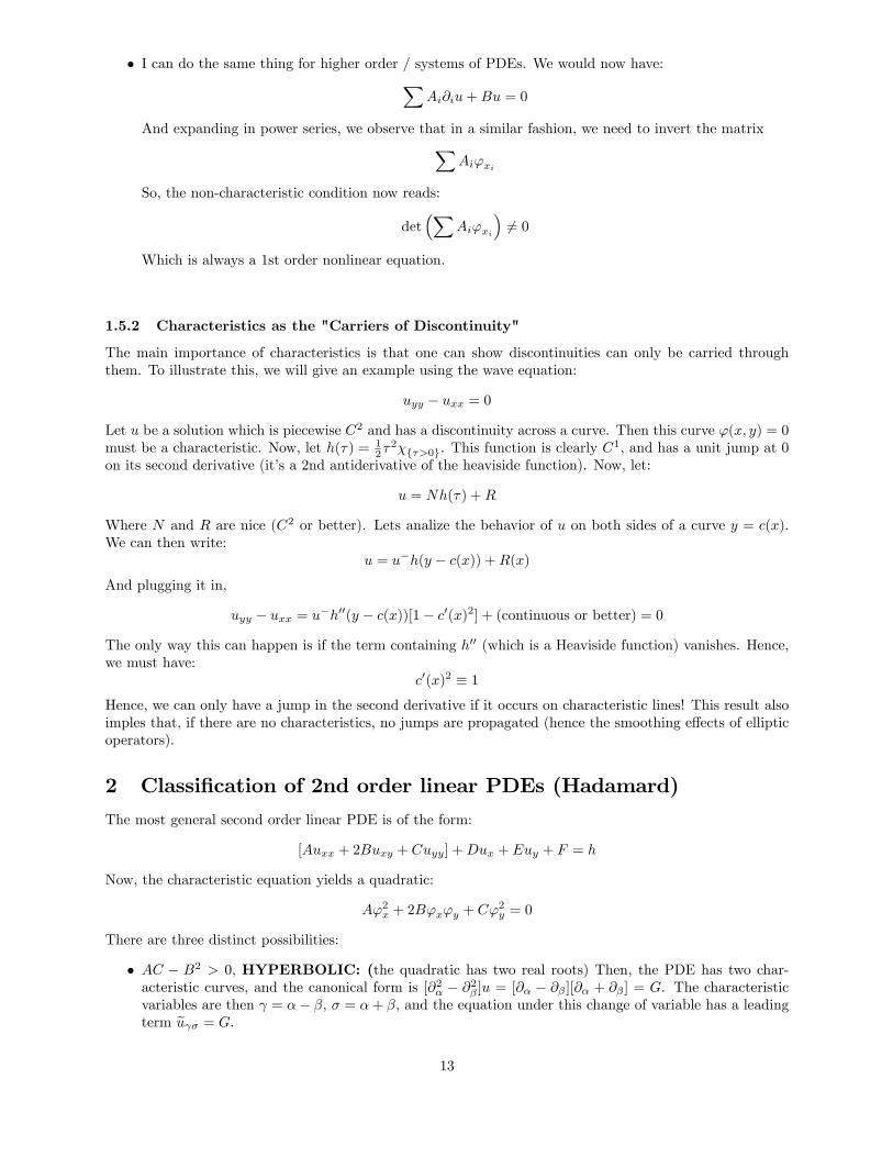
1.5.2 Characteristics as the "Carriers of Discontinuity"

The main importance of characteristics is that one can show discontinuities can only be carried throughthem. To illustrate this, we will give an example using the wave equation:

uyy � uxx = 0

Let u be a solution which is piecewise C2 and has a discontinuity across a curve. Then this curve '(x; y) = 0must be a characteristic. Now, let h(�) = 1

2�2�f�>0g. This function is clearly C

1, and has a unit jump at 0on its second derivative (it�s a 2nd antiderivative of the heaviside function). Now, let:

u = Nh(�) +R

Where N and R are nice (C2 or better). Lets analize the behavior of u on both sides of a curve y = c(x).We can then write:

u = u�h(y � c(x)) +R(x)And plugging it in,

uyy � uxx = u�h00(y � c(x))[1� c0(x)2] + (continuous or better) = 0

The only way this can happen is if the term containing h00 (which is a Heaviside function) vanishes. Hence,we must have:

c0(x)2 � 1Hence, we can only have a jump in the second derivative if it occurs on characteristic lines! This result alsoimples that, if there are no characteristics, no jumps are propagated (hence the smoothing e¤ects of ellipticoperators).

2 Classi�cation of 2nd order linear PDEs (Hadamard)

The most general second order linear PDE is of the form:

[Auxx + 2Buxy + Cuyy] +Dux + Euy + F = h

Now, the characteristic equation yields a quadratic:

A'2x + 2B'x'y + C'2y = 0

There are three distinct possibilities:

� AC � B2 > 0; HYPERBOLIC: (the quadratic has two real roots) Then, the PDE has two char-acteristic curves, and the canonical form is [@2� � @2� ]u = [@� � @� ][@� + @� ] = G. The characteristicvariables are then = �� �; � = �+ �, and the equation under this change of variable has a leadingterm eu � = G.

13

� AC�B2 < 0; ELLIPIC: (no real roots) Then, the PDE has no characteristic curves, and the canonicalform is [@2� + @

2� ]u = �u = G.

� AC�B2 = 0; PARABOLIC: (the quadratic has one real root) Then, the PDE has one characteristiccurve, and the canonical form is @2�u = G.

Not all equations �t in these categories, although there are ways of extending these to higher order PDEs.In general, each type of PDE has di¤erent properties that we want to study, and requires qualitativelydi¤erent approaches to �nd solutions.

Lecture 6 (05/02/09)

3 Hyperbolic Equations

3.1 Homogeneous equation

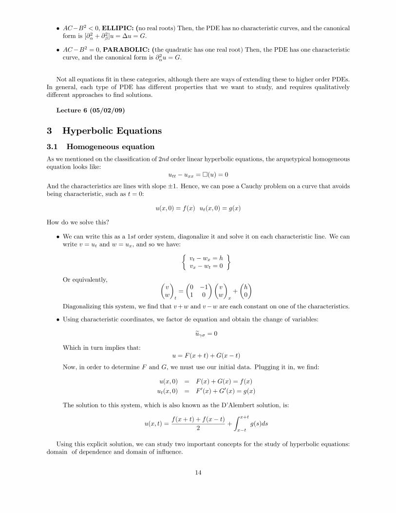
As we mentioned on the classi�cation of 2nd order linear hyperbolic equations, the arquetypical homogeneousequation looks like:

utt � uxx = �(u) = 0And the characteristics are lines with slope �1. Hence, we can pose a Cauchy problem on a curve that avoidsbeing characteristic, such as t = 0:

u(x; 0) = f(x) ut(x; 0) = g(x)

How do we solve this?

� We can write this as a 1st order system, diagonalize it and solve it on each characteristic line. We canwrite v = ut and w = ux, and so we have:�

vt � wx = hvx � wt = 0

�Or equivalently, �

vw

�t

=

�0 �11 0

��vw

�x

+

�h0

�Diagonalizing this system, we �nd that v+w and v�w are each constant on one of the characteristics.

� Using characteristic coordinates, we factor de equation and obtain the change of variables:

eu � = 0Which in turn implies that:

u = F (x+ t) +G(x� t)

Now, in order to determine F and G; we must use our initial data. Plugging it in, we �nd:

u(x; 0) = F (x) +G(x) = f(x)

ut(x; 0) = F 0(x) +G0(x) = g(x)

The solution to this system, which is also known as the D�Alembert solution, is:

u(x; t) =f(x+ t) + f(x� t)

2+

Z x+t

x�tg(s)ds

Using this explicit solution, we can study two important concepts for the study of hyperbolic equations:domain of dependence and domain of in�uence.

14

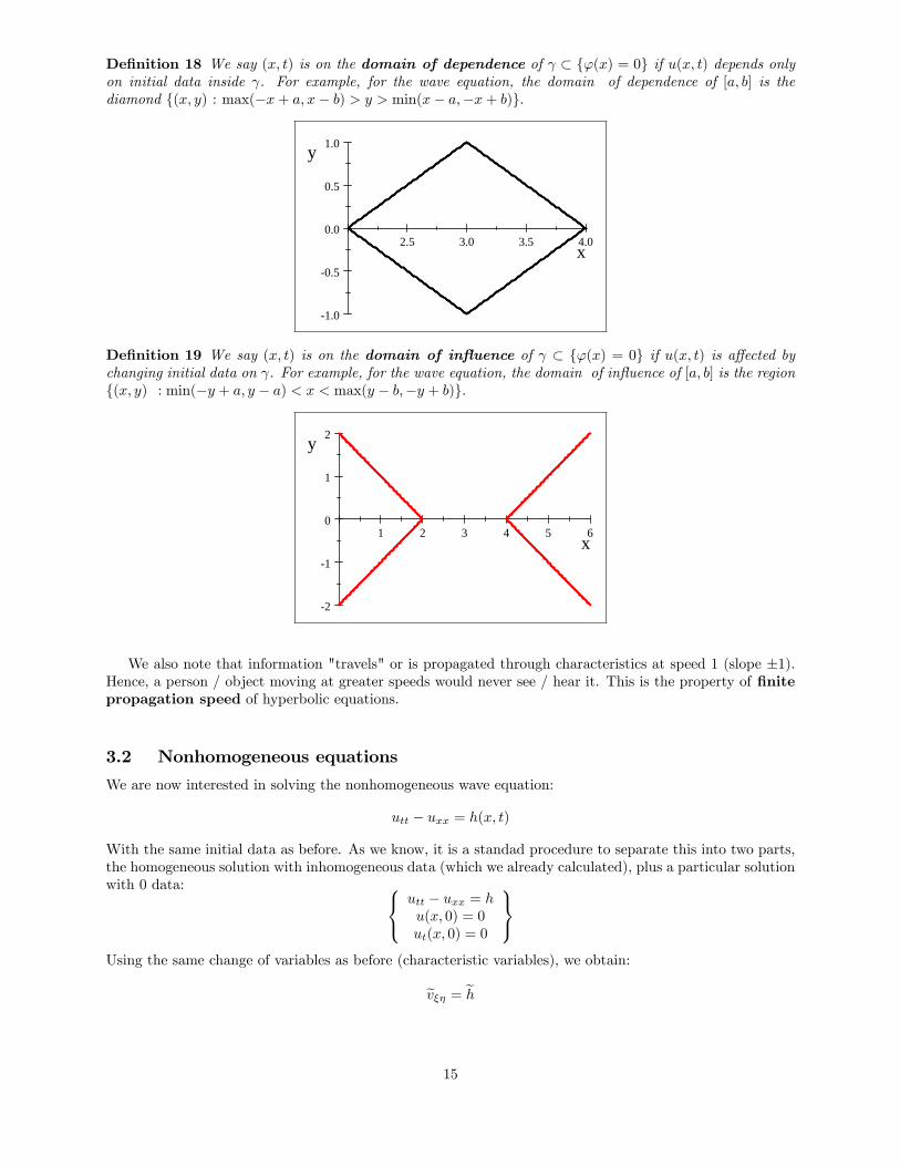
De�nition 18 We say (x; t) is on the domain of dependence of � f'(x) = 0g if u(x; t) depends onlyon initial data inside . For example, for the wave equation, the domain of dependence of [a; b] is thediamond f(x; y) : max(�x+ a; x� b) > y > min(x� a;�x+ b)g:

2.5 3.0 3.5 4.0

­1.0

­0.5

0.0

0.5

1.0

x

y

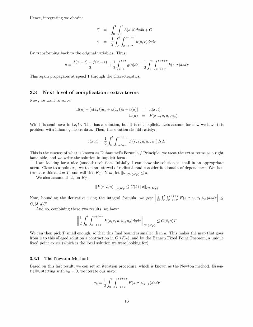
De�nition 19 We say (x; t) is on the domain of in�uence of � f'(x) = 0g if u(x; t) is a¤ected bychanging initial data on . For example, for the wave equation, the domain of in�uence of [a; b] is the regionf(x; y) : min(�y + a; y � a) < x < max(y � b;�y + b)g:

1 2 3 4 5 6

­2

­1

0

1

2

x

y

We also note that information "travels" or is propagated through characteristics at speed 1 (slope �1).Hence, a person / object moving at greater speeds would never see / hear it. This is the property of �nitepropagation speed of hyperbolic equations.

3.2 Nonhomogeneous equations

We are now interested in solving the nonhomogeneous wave equation:

utt � uxx = h(x; t)

With the same initial data as before. As we know, it is a standad procedure to separate this into two parts,the homogeneous solution with inhomogeneous data (which we already calculated), plus a particular solutionwith 0 data: 8<: utt � uxx = h

u(x; 0) = 0ut(x; 0) = 0

9=;Using the same change of variables as before (characteristic variables), we obtain:

ev�� = eh

15

Hence, integrating we obtain:

ev =

Z �

0

Z �

0

h(a; b)dadb+ C

v =1

2

Z t

0

Z x+t+�

x�t+�h(s; �)dsd�

By transforming back to the original variables. Thus,

u =f(x+ t) + f(x� t)

2+1

2

Z x+t

x�tg(s)ds+

1

2

Z t

0

Z x+t+�

x�t+�h(s; �)dsd�

This again propagates at speed 1 through the characteristics.

3.3 Next level of complication: extra terms

Now, we want to solve:

�(u) + [a(x; t)ux + b(x; t)u+ c(u)] = h(x; t)

�(u) = F (x; t; u; ut; ux)

Which is semilinear in (x; t). This has a solution, but it is not explicit. Lets assume for now we have thisproblem with inhomogeneous data. Then, the solution should satisfy:

u(x; t) =1

2

Z t

0

Z x+t+�

x�t+�F (s; � ; u; ut; ux)dsd�

This is the essense of what is known as Duhammel�s Formula / Principle: we treat the extra terms as a righthand side, and we write the solution in implicit form.I am looking for a nice (smooth) solution. Initially, I can show the solution is small in an appropriate

norm. Close to a point x0; we take an interval of radius �, and consider its domain of dependence. We thentruncate this at t = T , and call this KT . Now, let kukC1(KT )

� a;We also assume that, on KT ,

kF (x; t; u)k1;KT� C(�) kukC1(KT )

Now, bounding the derivative using the integral formula, we get:��� ddt R t0 R x+t+�x�t+� F (s; � ; u; ut; ux)dsd�

��� �C2(�; a)TAnd so, combining these two results, we have: 12

Z t

0

Z x+t+�

x�t+�F (s; � ; u; ut; ux)dsd�

C1(KT )

� C(�; a)T

We can then pick T small enough, so that this �nal bound is smaller than a. This makes the map that goesfrom u to this alleged solution a contraction in C1(KT ); and by the Banach Fixed Point Theorem, a unique�xed point exists (which is the local solution we were looking for).

3.3.1 The Newton Method

Based on this last result, we can set an iteration procedure, which is known as the Newton method. Essen-tially, starting with u0 = 0, we iterate our map:

uk =1

2

Z t

0

Z x+t+�

x�t+�F (s; � ; uk�1)dsd�

16

Now, we have a uniform bound kukkC1(KT )� a, and furthermore,

kuk+1 � ukkC1(KT )� C(a)T kF (uk)� F (uk�1)kC1(KT )

� C(a)M(a)T kuk � uk�1kC1(KT )

As we noted before, for T su¢ ciently small we have a contraction, and hence the sequence uk is Cauchy inC1(KT ). Thus, there exists a unique u such that uk ! u. We note here that u need not be C2; it dependson F and at best we can assert it is a weak solution to the original di¤erential equation.

3.4 Hyperbolic systems

Now, think about the hyperbolic system:�ut + (1 + u

2)ux = v2

vt � vx = u2

�Can we still perform some kind of iteration procedure / �xed point argument? This is a quasilinear problem,and we can write it as ut +A(u)ux = f(x), where u is a vector and A(u) is a matrix. We can then �nd thecondition for a surface to be characteristic: if we have the surface '(x; t) = 0, it is characteristic if and onlyif

det(A'x + 'tI) = 0

That is, if we cannot invert the leading term in our expansion / cannot compute derivatives of u from data.Then, if this surface is given by the equation x = s(t), this implies:

det(A+ds

dtI) = 0

That is, �ds

dt= �(u) : �(u) 2 �(A(u))

�Are the characteristic curves for this equation. If all eigenvalues are real and distinct, and I have a full setof eigenvectors, we call the equation strictly hyperbolic. If in addition, A is symmetric, we call this asymmetric hyperbolic system. We note that the method of characteristics requires us to diagonalize thismatrix, in order to work in characteristic coordinates.

3.4.1 Newton Method (revisited)

Now, we will see that the same iteration procedure applies for 1st order hyperbolic systems.

� Say we have:

ut +A(x; t)ux = f(x; t; u)

u(x; 0) = u0(x)

t = 0 is not a characteristic and the system is strictly hyperbolic. "So you say, this is too complicated,�rst I�ll diagonalize it". After a change of variables,�

@ua@t

+ �a(x; t)ua = fa(x; t; u)

�Na=1

� We then solve the system of ODEs dxadt = �a(x; t); xa(0) = x0, Dtua = fa.

If we start on x0; this is ging to give me solutions "all over the place", since each coordinate travels ondi¤erent curves. We cannot solve this as a system of ODEs. What do I do? I start with (x; t) a point closeenough to the x axis, and ask what is u(x; t). If all curves intersect it, then I am �ne.

17

� So, choose � small enough so that the Implicit Function Theorem guarantees that all characteristiccurves a intersect the x axis. That is: a is a map from x0 to x; and I need to invert it. I knowd kdx0

= 1 at time t = 0, so for t � � small enough, the derivative remains positive and this inversion ispossible.

� We then restrict the region in which we are solving. If M = maxt��f�kg and m = mint��f�kg; for asmall enough interval [x1; x2] we can consider the trapezium consisting of t 2 (0; �) and bounded bythe line of maximum slope / speed M on x1 and that of minimum slope / speed m on x2 (that way,we ensure the solution inside depends only on the data in [x1; x2]; that is, we are inside this interval�sdomain of dependence).

� Now, my iteration procedure reads: �d adt = �a( a; t)

Dtuma = fa(x; t; u

m�1)

�This de�nes a sequence um in , and using the same argument as before we can make this into acontraction mapping for � small enough. Hence, we have proved the existence of a solution with dataon t = 0, and u0 2 C1 implies the local solution u 2 C1().

� Finally, to check local well-posedness, we have to check that the solution map u0 ! S(u0) = 0 iscontinuous from C1 to itself. This of course depends strongly on the topologies of the spaces we takeour data and our solution to lie on.

� We �nally note that, if we now make A depend on u; we get a quasilinear equation. In that case, �adepends on u, but nothing essential in the previous argument changes.

Lecture 7 (10/02/09)

Part II

Background MaterialHere are some results which are needed to build analytical tools and work with PDEs from a more general/ rigorous standpoint:

3.5 Fourier Transforms

The Fourier Transform is one of the most useful operators in mathematical analysis. In order to extend itfrom the function spaces where it is usually de�ned (say, L1) to L2 and spaces of distributions, it is relevant�rst to introduce the space of rapidly decaying smooth functions:

De�nition 20 (Schwartz Space) We de�ne S(Rd) = ff 2 C1(Rd) : x�D�f

1 < C�;� 8�; �g

Proposition 21 Let f 2 S; then the Fourier Transform de�ned by

bf(�) = 1

(2�)d=2

Ze�ix

>�f(x)dx

is well de�ned, and moreover, bf 2 S. The converse is also true.Proposition 22 Two key properties of the fourier transform that are linked to the previous result are thosewhich relate derivatives and multiplication by powers. That is,

D��bf(�) = \[(�ix)�f ](�)dD�

xf(�) = (i�)� bf(�)18

Proposition 23 8f 2 S(Rd),kfkL2 =

bf L2

Proof. The core of the proof is to use a limit with a Gaussian distribution function, using it as an approxi-mate identity. That is, we have: bf

L2= lim

"!0

Z Z Ze�"j�j

2

f(x)e�ix>�f(y)eiy

>�dxdyd�

Applying Fubini, we integrate exp(�" jxj2+i(y�x)>�) with respect to �; and obtainG"(x�y) = 1(2�")d=2

exp(� jx�yj24" );

which is a Gaussian distribution function with variance ": We can also see it as an approximate identity.Now,

lim"!0

Z ZG"(x� y)f(x)f(y)dydx =

Zf(y)f(y)dy = kfkL2

Since the convolution of f with an approximate identity in L2 converges to f .This result is usually known as the Plancherel theorem, and since S is dense in L2; it allows us to de�ne

the fourier transform F (f) = bf for any f 2 L2.3.6 Sobolev Spaces Hk()

Now that we can use the fourier transform in L2, we would like to de�ne subspaces of functions which havederivatives (in a generalized sense) in L2. In the case of the space of Schwartz, we saw bounding derivativesin space was equivalent to bounding powers in the fourier domain. Hence, it is natural to de�ne:

De�nition 24 (Sobolev Space Hs()) Given s > 0 (not necessarily an integer), we de�ne the space Hs() =

fu 2 L2() : (1 + k�k2)s=2bu(�) 2 L2()g. This is a Hilbert space, with the normkukHs =

(1 + k�k2)s=2bu L2

For s = k integer, we can also de�ne this space as fu 2 L2 : D�u 2 L2 8 j�j � kg; and equip it with theequivalent norm:

kuk2k; =Xj�j�k

kD�uk2L2

It is clear that H0 = L2; and that Hs is a closed subspace of L2 for s > 0. What would Hs() be fors < 0? (It is the dual space of H�s

0 ()).

Example 25 H�2(R2) is the space of objects which on the Fourier domain are proportional / with growthlike 1, since: Z

R2(1 + k�k2)�2dx <1

Similarly, objects in H�3(R2) would be asymptotically proportional to � on the fourier domain.

A fair question is if there are functions with these behavior, and the answer is no. To de�ne these objectsproperly, we must interpret them as functionals of a dual space, which is the space of distributions (orgeneralized functions). We need these functions to study such things as di¤erential operators of functions inL2.

Lecture 8 (12/02/09)

19

3.7 Distributions

In the same way we have de�ned the Hs Sobolev spaces with negative s (which can be interpreted as dualspaces), we can de�ne spaces of generalized functions by taking the dual of spaces such as S.

De�nition 26 The space S� with the corresponding weak� topology is known as the space of tempered dis-tributions, and it can be identi�ed with slowly growing functions. By duality and using the weak Parsevallemma, we can de�ne the Fourier Transform on S� by:

hF (T ); �i =DT; b�E 8� 2 S

De�nition 27 The space C10 () = D(); known as the space of test functions, is the space of C1 funtionswith compact support in . We can immediately see that D � S.

De�nition 28 The space D� is what we now as the space of distributions, or generalized functions.

We then have the following embeddings:

C10 � S � :: � H1 � L2 � H�1 � :: � S� � D�

In order to work with these spaces, we must �rst determine what is the topology and convergence in thespace of test functions. This is a union of Fréchet spaces, and we say f�ng � D() is convergent to � if9K �� (compact) such that supp(un) � K 8n � n0 and D��n ! D�� uniformly on K.

Proposition 29 Then for every element T 2 D�, we have that 8K compact set of , 9 N(K) such that

jT (u)j � CK kukCN (K)

When this N is independent of K; we say T is a distribution of order N:

Proof. We show this by contradiction. Lets assume 9K0 a compact set such that 8N 2 N 9 uN 2 D(K0)such that kuNkCN (K0)

= 1 and jT (uN )j � N . But then, vN = uN= jT (uN )j is such that:

kvNkCN � 1

N(hence vN ! 0 in D())

T (vN ) = 1 8N

Which contradicts the fact that T 2 D�.

Why do we like the Fourier Transform de�nition for Sobolev spaces? Lets show an embedding result: Lets > 0; f 2 Hs(Rd). Then:

kfk1 � bf

1� 1

(1 + k�k2)s(1 + k�k2)s bf

� 1

(1 + k�k2)s

2

(1 + k�k2)s bf 2

= (1 + k�k2)�s

2kfkHs(Rd)

Now, (1 + k�k2)�s

2is �nite if and only if s > d=2. In that case, we have a continuous embedding of

Hs(Rd) ,! C(Rd). Using a similar procedure, we can also conclude that, when s > d=2 + N , we have anembedding Hs(Rd) ,! CN (Rd). These results are very important, since they link Sobolev spaces (which wecan work with on a very general setting) to classic spaces, and thus are useful to determine the regularity ofweak solutions of PDEs.

Remark 30 Now, let T 2 D� of order N . Then, by the previous result, we have that for u 2 Hs(Rd); withs > d=2 +N we have:

jT (u)j � C kukCN (K) � eC kukHs(Rd)

Hence, T 2 H�s for all such s. In particular, N counts the number of derivatives I need to use.

20

Proposition 31 Any measures that assign �nite values to compact sets (Radon measures) are distributions.For example, the dirac mass �0(�) = �(0).

3.7.1 Weak derivative and other operations on D�

We can now extend the notion of derivative to the space of distributions (as can be seen, most operationscan be succesfully extended by duality arguments). This notion of weak derivative will give us a precise wayto work with weak solutions of PDEs.

De�nition 32 Let T 2 D�: Then, the weak derivative D�T is de�ned by its action on � 2 D():

hD�T; �i = (�1)j�j hT;D��i

This is a direct generalization of what we would get using integration by parts. In this case, both notionsof derivative coincide.

Other operations are allowed on D�; as long as we are careful:

� (multiplication by a function) Let 2 C1. Then I can de�ne T by duality: h T; �i = hT; �i.Leibniz rules applies when considering this in combination with the weak derivative.

� (convolution) it is possible to extend the operation of convolution quite a bit, but it requires severalsteps. First, we remember some of the things we know about convolution:

� If f 2 CK0 and /g 2 CL0 ; then f � g 2 CmaxfK;Lg0 and supp(f � g) �supp(f)+supp(g): (In general,

it always "inherits" the best behavior)

� \(f � g) = bfbgNow, let T 2 D�. Can I convolve it with ' 2 D()? If it made sense to write the integral, we would

have: ZT (y)'(x� y)dy = hT; �x(')i

Now, suppose ' 2 Ck0 ; I can talk about T ('��). However, if I remove the compact support, this is no longertrue.

Support of a Distribution In order to further extend the notion of convolution, we need to know what itmeans for a distribution to vanish, or equivalently, what the support of a distribution means. Again drawingintuition from the cases in which the integral makes sense, we know that

Rfg = 0 whenever the supports of

f and g are disjoint. Hence, we say T is supported on U closed set if hT; �i = 0 8� 2 D(U c).Now, if T has compact support, we can talk about T � S; with S another distribution. We can do this

because T � ' 2 D(), and so T � S(') = S(T � ') is well de�ned.

Proposition 33 If T is a distribution supported at x = 0, then

T =Xj�j�N

C�D��0

An application of this is the following: Let u 2 S�; and �2bu � 0. Hence, bu is only supported at 0, so wehave:

u =Xj�j�N

C�D��0

We would like to conclude that C2; ::; Ck = 0. We have:Z�2bub� = 0

Now, we can construct � such that b�(0) 6= 0 and �0(0) = �00(0) = ::0. Then, by plugging it in, we can showC2 = C3 = :: = 0 (�2 only survives when applying 2 derivatives or less). Hence, bu = C0� + C1�

0. (Checklater)

21