PART Ill

QUANTITATIVE METHODS OF RISK ASSESSMENT -I : Consequence analysis

INTRODUCTION TO PART Ill

This part is devoted to the quantitative methods we have developed for analyzing some of the consequences if an accident takes place in a chemical process industry. Chapters 6-8 describe a model for heavy gas dispersion, and its applications. The model helps in Arecasting the pattern of dispersion and consequently the area-of-impact, when heavy gases are released voluntarily or involuntarily. We have also presented a methodology for controlling dispersion so as to reduce its adverse impacts (Chapters 7-8).

Chapters 9 and 10 presenksystems developed by us in simulating and forecasting consequences of release of toxic gases , fires, and explosions.

All of these studies have either been published or in press. We have reproduced full texts of the published/accepted papers in the forms of Chapters 6-10.

Chapter 6

MODELLING AND SIMULATION OF HEAVY GAS DISPERSION ON THE BASIS OF MODIFICATIONS IN PLUME PATH THEORY'

An analytical model for heavy gas dispersion based on the modifications in plume path theory has been developed. The model takes into account the variations in temperature, density, and specific heat during the movement of heavy gas plume.

The model has been tested for three hazardous gases - chlorine, natural gas and liquefied petroleum gas. The results have been compared with the recently generated experimental data as also with the outputs of other models. A good agreement is observed qualitatively as well as quantitatively. A study has also been cam'ed out to simulate the effect of the wind

speed, density of the gas, end venting speed on dispersion. Based on the simulation study a set of empirical equations have been developed. The equations are validated by theoretical as well as experimental studies.

INTRODUCTION

Modelling of the dispersion of the 'dense' gases - gases with density higher than air - has been assuming ever greater importance as many of the hazardous gases (chlorine, hydrogen fluoride, liquefied petroleum gas) are denser than air. Numerous air pollution models, which were developed for lighter-than-air or light-as-air gases, have not been successful with dense gases; accentuating the need for mathematical models appropriate for dense gas dispersion. In recent years, a few mathematical models have

' Communicated to Atmorpheric Environment, USA

been proposed for the study of heavy gas dispersion - notably by Ooms et a/. (1974), Ooms and Duijm (19831, Colenbrander (1980), Eidsvik (1980), Ermak and Chan (1985), Van Ulden (1983.1987), Langlo and Schatzmann (1991) and Deaves (1983,1992).

One of the first attempts to model the heavy gas dispersion was made by Ooms et a/.. (1974). They proposed an analytical model based on using the conventional transport phenomena and the plume path theory (Ooms, 1972). Later Colenbrander (1980) proposed slab (continuous release box) model which assumes normal distribution of concentration within the slab. Around the same time Eidsvik (1980) proposed a refined box model with equations modified to estimate vertical entrainment of air. Van Ulden (1983), Van Ulden and Holtslag (1985), and Van Ulden (1987) used K-theory with atmospheric scaling parameters to model heavy gas dispersion. Ermak and Chan (1985) proposed a model based on the turbulence dissipation and boundary layer parameters. In subsequent years, Langlo and Schatzmann (1991) modelled the heavy gas dispersion using Langrangian approach based on similarity theory. Deaves (1992) modelled the atmospheric turbulence and analysed the way it affects dense gas dispersion. He also used K-theory and employed more extensive meteorological data than the other models did : wind profile, turbulence and boundary layer profiles.

Surprisingly in the present age of computer-based application software, very few such models have been proposed. They include finite difference models which use K-theory : MARIAH ( Taft et a/. 1983),SMART (Tran and Liu , 1981). SIGMET (England et a/. 1978; Havens, 1982) and MERCUR-GL (Riou, 1986), or box model such as HEGADAS ( Colenbrander . 1980; Puttock , 1986). Of these the last named is the most often cited one. The output of these models are well tested with experimental values and are found to be in fairly good agreement.

Although the above mentioned models have been reasonably successful in some cases, they are limited in scope and have found applicability in only certain specific conditions only. In this paper we present a model based on plume path theory (PPT) which, we hope, may enrich the existing repertoire of the heavy gas dispersion models presently available.

Plume path theory (PPT) was proposed by Ooms (1972) and has been used mainly to calculate the plume path of the lighter-than-air and light-as-air gases escaping from the stacks into the atmosphere at atmospheric temperature and pressure. Later this theory was extended to 'heavy' gases (of density higher than air; Ooms eta/. 1974) with a number of assumptions, Numerous applications of the PPT have been reported for example, Rottman et a/. (1985) and McQuaid (1986) have used the theory for analysing toxic gas dispersion; Niewstadt (1982,1992), Blewitt et a/. (1 987) and Weil (1988) have used the same for vapour cloud modelling; and Ooms and Duijm (1983) have used the theory to estimate the dispersion of heavy gases coming out of the stacks with high momentum. The theory has also been the basis of the commercial packages PLUME and HFPLUME. In spite of the obvious potential of Ooms' theory, it has not enjoyed wider applicability because the main assumptions have not yet been overcome. The authors of this paper have recently modified Oorns's theory to significantly enhance its range, accuracy, and precision. Most importantly we have enabled application of the theory to 'heavy gases' which is a much less explored domain of air quality modelling than the dispersion of the lighter-than-air or light-as-air gases.

Based on the theory PPT (Ooms, 1972; Ooms et a/. 1974; Ooms and Duijm, 1983) is a simple approach based on the fundamental principles of fluid dynamics such as Fick's law of diffusion, turbulent kinetic energy and fluid flow. It is based on the assumption that the density and the specific heat of a gas do not differ significantly from that of air. In dispersion calculations, it neglects density spread as well as buoyancy effect. However, these a~S~mpt i0ns do not hold true for heavy gas dispersion. In the present paper we have modified PPT in an attempt to make it suitable to model heavy gas dispersion. Some empirical correlations have also been developed to show the dependency of plume variables (concentration, density, plume width, plume velocity) on atmospheric operating variables such as wind velocity, venting velocity and density difference. The applicability of the model developed by us has been demonstrated.

MATHEMATICAL REPRESENTATION

In its original f 0 n ( O O ~ S , 1972) plume path theory takes into account only plume dimensions namely velocity and concentration. Later it was modified to take into account density and specific heat variations(0oms and Mahiue,1974). Ooms et a/. (1974) demonstrated its application to the modelling of venting gases heavier than air at high temperature. However, the modified PPT was based on a number of assumptions (Table 1). The present work is an attempt to make the existing theory more reliable by redefining the assumptions (Table 1) and developing empirical relations to estimate the effect of release and atmospheric parameters on dispersion.

Profiles

Let s, r, and 4 be the plume co-ordinates at the plume axis as shown in Figure 1. These co-ordinates are related to the horizontal and vertical axis as :

dx/ds= cos4 dz/ds= sin$ I (1)

In the earlier form of PPT (Ooms and co-workers,l972; 1974; 1983) only three parameters (u.p,c) have been considered as significant. In the present work temperature also has been taken as one of the dominant parameters, Incorporating the aspects of plume density, temperature and specific heat, the plume characteristics can be written as:

u(s,r,cp) = u,coscp + uSexp(-?lb;) (2)

p(s,r,cp) = pa + p'exp(-?lh2b,2) (3)

c(s,r,cp) = c' ' exp(-?li,2'bz) (4

T(s,r,cp) = ~ , + e x ~ ( - r ? ~ ? b ~ ) (5)

Where u(s,r,$),.p(s,r,$),c(s,r,$) represent the values of the variables at an arbitrary point in the plume; lj',r ,c' denote the values of variables relative to the surroundings on the plume axis in the direction at a tangent to the plume axis.; and b represents the local characteristic width of the plume, in the present study it is equal to the radius of plume (b12).

Plume path

As the plume moves through the atmosphere, air is entrained. Getting a precise mathematical description of this entrainment is one of the most difficult problems in the air

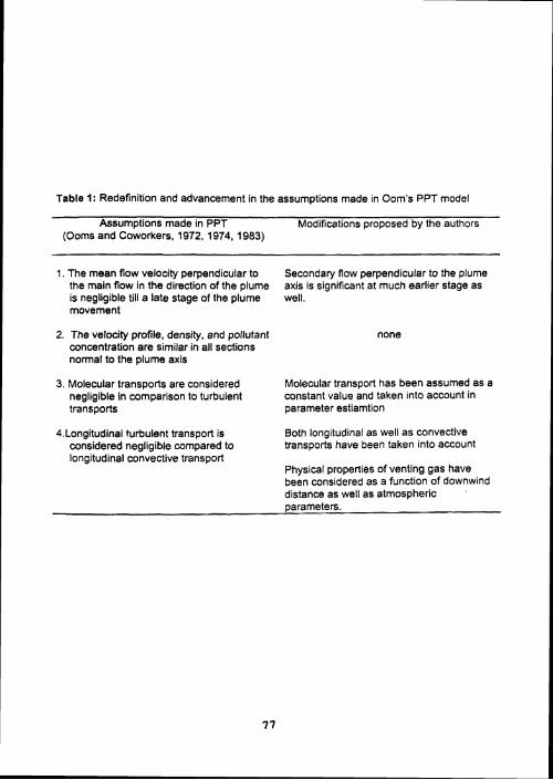
Table 1: Redefinition and advancement in the assumptions made in Oom's PPT model

Assumptions made in PPT Modifications proposed by the authors (Ooms and Coworkers, 1972, 1974, 1983)

1. The mean flow velocity perpendicular to Secondary Row perpendicular to the plume the main flow in the direction of the plume axis is significant at much earlier stage as is negligible till a late stage of the plume well. movement

2. The velocity profile, density, and pollutant concentration are similar in all sections normal to the plume axis

none

3. Molecular transports are considered Molecular transport has been assumed as a negligible in comparison to turbulent constant value and taken into account in transports parameter estiamtion

4.Longitudinal turbulent transport is Both longitudinal as well as convective considered negligible compared to transports have been taken into account longitudinal convective transport

Physical properties of venting gas have been considered as a function of downwind distance as well as atmospheric parameters.

Figure 1. The plume coordinates as used in the present study

pollution we have following

modelling (Hawthrone-1955, Abraham-1970. Briggs-1984, McQuaid-1986). Here tried to represent the entrainment in terms of mass flow equations keeping the facts in mind :

a) in the vicinity of vent or release point venting velocity is higher than wind velocity,

b) at a sufficiently long distance downwind, the velocity of the plume may equal the wind velocity,

c) atmospheric turbulence is one of the most effective factors causing entrainment.

These three facts have been taken into account independently by Abraham (1970), and recently by Briggs (1984). Fay and Zemba (1985) who proposed different flow equations for each type of entrainment. The final mass flow equation will be a combination of these three entrainment modes with modified profiles of plume characteristic parameters. The mass flow equation can be written as;

where,

2nbsp, a,lu'~ represents the entrainment due to the jet release of gas.

2nbSpaa2u,l~incpl~~scp represents the entrainment in a thermal stagnant atmosphere

2nb,pa a3u represents entrainment due to atmospheric turbulence.

The values of entrainment coefficient a, ~0.0762, a, = 0.61, and a, = 1.0 have been taken from Fay and Zemba (1985,1986), Krogstad and Jacobsen (1991).

Component mass balance

The component mass balance over a cross section of plume is worked out as :

d( jcu2nrdr) l ds = 0 (7)

This implies that no gas is assumed to be present in the atmosphere outside the plume.

Momentum balance

In plume, the momentum occurs mainly due to

a) entrainment of air,

b) force exerted by wind.

Keeping these in view the momentum balance equation in the downwind direction can be written as :

d( j(pu2coscp2xrdr)) I d ~ = 2 n b , ~ ~ u ~ { u , ~ u ' ~ + a ~ ~ s i n c p ~ c o s c p + a 3 u ) (8)

Where,

27ib,p,~a{al~u'~+a,u~sincp~coscPta3~} represents the increase in momentum due to inflow of air from the surrounding atmosphere.

cdnbSp,u,2lsinJ9 represents the increase in impulse due to the drag force exerted by the wind on the plume.

The momentum balance in the cross wind direct~on is a combination of

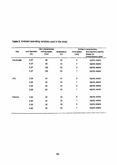
Table 2. Ambient operating variables used in the study

Vent characteristic Ambient characteristics Gas vent diameter venting speed temperature wind speed atornospheric stabil~ty

(m) (WS) (c) ( d s ) (based on meteorolog~cai data)

Natural gas 0.37 95 50 5 slightly stable

0.37 95 50 7 slightly stable

0.37 125 50 5 slightly stable

0.37 125 50 7 slightly stable

LPG

Chlorine

0.25 45 40 5 slightly stable

0.25 45 40 7 slightly stable

0.25 63 40 5 slightly stable

0.25 63 40 7 slightly stable

0.20 25 35 5 slightly stable

0.20 25 35 7 slightly stable

0.20 35 35 5 slightly stable

0.20 35 35 7 slightly stable

density spread,

drag force exerted by wind.

The final balance equation can be written as :

d( I(pu21sincp12nrdr))lds = k(p-p,)2nrdr - ~ ~ ~ b , p , ~ ~ s i n ~ ~ c o s ~ (9) The first term ~(puzlsincp12nrdr) represents density spread while second term

c,nb,p,~,~sin~~coscp represents the impulse due to drag force exerted by wind.

Energy balance

The energy balance for the plume implies that the amount of heat emitted by the gas per unit time is conserved with respect to a chosen reference. So, for a reference temperature T the energy balance equation can be written as:

d( Ipucp(T-Ta,)2nrdr) 1 ds = 2nb,p,cp,(~,-~,,){a,~u'~+a,u,~~in~~cos~~u} (10) If it is assumed that air and vent gas obey ideal gas law, then the temperatures (plume

and air temperature) can be expressed as

T = M,P/(Rp) and T, = M,P/(Rp,) (11) Where, M, and M, represents molecular weight of plume and air respectively at any

point in the plume. As molecular weight and specific heat differ, unlike what was assumed in the original PPT (Ooms-1972), these variables can be expressed as:

M, = M,cT I (c,T,) + M,,(l-cT/(c,T,) ) (12)

Combining the above energy balance equations with molecular weight variation and specific heat variation, the final equation can be written as :

SOLUTION OF THE MODEL

By substituting the similarity profile to these conservation equations, integrals can be calculated by using a suitable numerical integration technique-here we have used Siphons-113 technique. Sets of non-linear simultaneous equations have been solved by using Newton-Raphson method (Carnahan-1969) coupled with L-U decomposition (Camahan-1969) technique. The model has been solved for three different gases and for different atmospheric operating conditions as presented in Table 2.

Experimental studies

An extensive study to measure the quality of stack emissions and the behaviour of the P ~ W formed when ammonia is released from a pressurised storage vessel was conducted at Manali (near Madras, southern peninsula of India). The initial and boundary conditions of the release are given in Table 3. The study area has flat terrain and is made up of rural habitat. The study included meteorological parameters (vertical temperature Profile, vertical as well as horizontal wind velocity profile), air quality (concentration

Table 3. The initial and boundary conditions for release of ammonia from pressurized vessel through vent valve

Parameters Values

Storage capacity 200 tons

Storage temperature 45 OC

Storage pressure 1625 kPa

Height of the vessel 10.5 rn Height of vent pipe 2.5 m

Vent diameter 0.2 m

Ambient temperature 27 OC

Ambient pressure 107.3 kPa

Wind speed (at 10 rn) 5.5 mls

Wind direction North-West

Terrain of the area Flat rural area with a roughness height of 1.2 m

profiles), and behaviour of the plumes (of heavier-than-air as well as heavy-as-air gases) under different sets of conditions influencing dispersion for a continuous as well as an instantaneous release. The following characteristics of the plume were studied measuring

parameters such as; temperature variation within the plume, concentration profiles in the cross wind and downwind directions, plume width, plume height, and the effect of the meteorological Parameters on the plume behaviour. A gist of the experimental results obtained in the present Study is presented in Table 4.

RESULTS and DISCUSSION

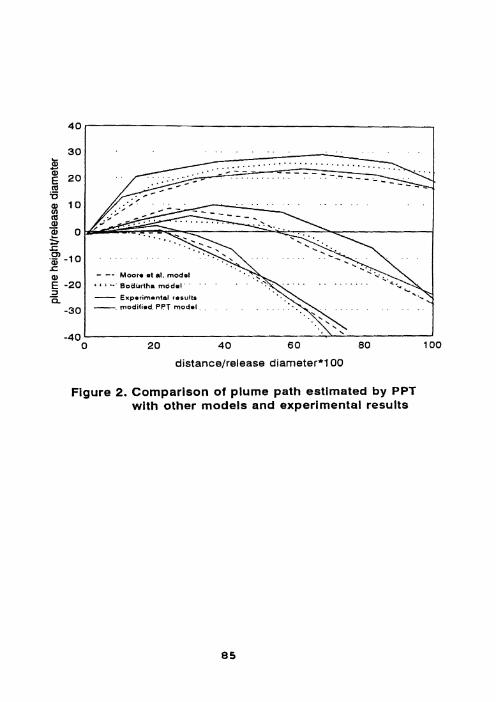
The comparison of the plume path (height of plume rise) obtained by our model with the results reported by Bodurtha (1961) Moore et el. (1988) and our own recent experimental studies are presented in Figure 2. Good, qualitative as well as quantitative, agreements have been observed.

The temperature and the plume velocity variations have also been compared with that of the experimental data (Table 4), and a fairly good agreement has been observed (Figures 3 and 4). When the concentration profile obtained by the present model (for release of ammonia) is compared with our experimental results (Figure 5) the predicted results are seen to lie within the confidence interval of 40-50%, a match acceptable for air pollution models.

The simulation study reveals that the plume width and the plume velocity both increase in the downwind direction, while density of the plume, temperature of the gas (above atmospheric temperature) and gas concentration ail decrease downwind. We see that the trend diminishes as the distance of travel of the plume increases. This has been observed for all the three gases studied (natural gas, LPG, chlorine). The observations on the individual gases are summarised below.

Natural gas

Figure 6 shows the behaviour of plume variables (dimensionless form) in downwind direction due to the change ( step increase) in wind and venting speeds. An increase in the w~nd speed causes an increase in the plume velocity and the plume width. A similar trend is also observed for an increase in the venting speed. However, the trend is more marked in the case of increase in the venting velocity compared to the increase in wind speed. Perhaps high venting speed creates high turbulence and wake formations in the atmosphere which consequently lead to the rapid entrainment of air and swift dispersion too. Wind speed effects the downwind transportation of the plume more strongly than it does the entrainment of air and its dispersion. As the density of the gas ( vapour density '1.34) is not much higher than air a fast response due to a change in the controlling Parameters viz, wind velocity and venting velocity, has been observed. For example, a venting velocity of 125 mls ( mass release rate 10 kgls for 5 min) covers a smaller area under flammability limits compared to a venting velocity of 95 mls ( mass release rate 5 kgls for 10 min) under high wind (15 m/s). This reveals that a high release (venting) velocity of this gas for shorter periods is safer than a slow release under unstable conditions for longer duration.

Table 4. Experimental results obtained in the present study

Down wind Plume velocity Ground level Plume with Plume

distance meters meters concentration meters temperature

, . . . . . .

Moore m t al. model

Bodurtha m6d.I

modified, PPT model

Figure 2. Comparison of plume path estimated by PPT with other models and experimental results

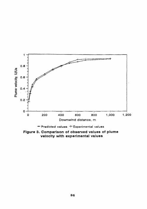
0 200 400 600 800 1,000 1,200

Downwind distance, m

- Predicted values -Experimental values

Figure 3. Comparison of observed values of plume velocity with experimental values

0.5 1 0 200 400 600 800 1,000 1,200

Downwind distance, m

- Predicted values i Experimental values

Figure 4. Comparison of observed values of plume temperature with experimental values

0 0.1 0.2 0.3 0.4 0.5 0.6 0.7 0.8 0.9 1

Observed values, C/Cmax

Figure 5. Comparison of concentration of gas in the plume with experimental values (venting of ammonia)

Distance from the venting point, rn

Figure 6. Impact of a 40% change in wind speed (from 5 m/s to 7 m/s) as compared to the impact of 40% change in venting speed (from 95 m/s to 125 m/s) on three plume variables (Natural gas)

iique5ed petroleum gas (LPG)

The pattern of dispersion of LPG is by and large simiiar to the pattern of dispersion of natural gas discussed above. However a iow venting speed (45 m/s) and a higher density causes slower dispersion. It is evident from Figure 7 that at any distance along ihe downwind direction, piurne velocity and the concentration of gas in the plume are higher while plume width is less due to an increase in the wind speed when compared with the increase in venting speed. Thus high venting speed has stronger influence on the entrainment of air and the plume width leading to faster dispersion. But high wind speed also transports the plume to a larger disiance with higher velocity.

Chlorine

Of the three hazardous gases discussed in this work, chlorine has by far the slowest rate of dispersion. Otherwise the trend observed with chlorine is broadly simiiar to the trends seen with the other two gases. As is evident from Figure 8 the dispersion increases with an increase in the ~vind speed and is faster with the higher venting speeds. For any given distance, the concentration of chlorine is higher and the plume velocity is lower compared to the other two gases. As chlorine gas is the most toxic of the three gases studied and is also the most sluggish to disperse, lethal concentration of this gas can easily build up over large areas and persist for long durations over larger areas.

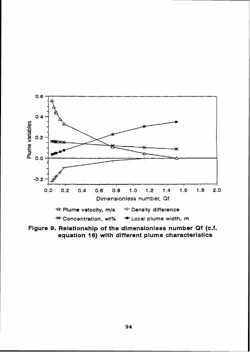
parametric effect To generalise the effect of wind speed, density and venting speed on the plume paih, we have developed some empirical equations. These equations directly predict the behaviour of plume variables (gas concentration in plume, plume density, local plume width, plume veiocity) with other operating vzriabies viz : density of gas, venting speed, etc.

For this purpose a dimensionless number Qf has been defined as:

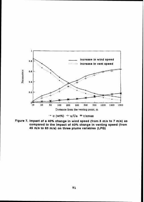
- increase in wind speed . . . . . . - increase in vent speed

D~stance horn the venting point, m

Figure 7. Impact of a 40% change in wind speed (from 5 m/s to 7 m/s) as compared to the impact of 40% change in venting speed (from 45 rn/s to 63 m/s) on three plume variables (LPG)

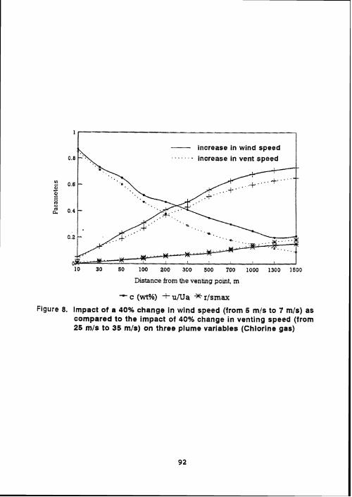
- increase in wind speed - . . . . . . increase in vent speed

10 30 SO 100 200 300 SO0 700 1000 1300 1500

Distance from the venhng point, m

Figure 8. Impact of a 40% change in wind speed (from 5 m/s to 7 mls) as compared to the impact of 40% change in venting speed (from 25 m/s to 35 m/s) on three plume variables (Chlorine gas)

The equations have been validated with experimental values. A plot representing different plume variables at Y axis with dimensionless number 0, is shown in Figure 9. It can be seen that with an increase in Qf , variables like plume width and plume velocity (shown on Y axis) increase while gas concentration and density difference both decrease.

CONCLUSION

The plume path theory as modified by us gives satisfactory results for the dispersion of heavy gases. It also enables simulation of plume profiles along the cross section of plume as well as in the downwind directions. The empirical equations developed by us on the basis of the present model, we hope, would prove to be helpful in air-pollution studies, as they can predict responses to the different ambient operating conditions over the plume variables (concentration, density, local width, temp etc.) with relative ease and fair accuracy.

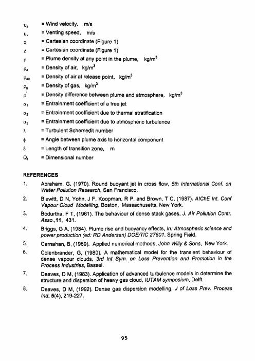
LIST OF SYMBOLS

b, = Local characteristics width, m

c = Concentration of gas at any point inside the plume, kg/m3

c' = Concentration of gas on the plume axis, kg/m3

C, = Concentration at out let, kglm3

cp, = Specific heat at outlet, JIkgIK

cp = Specific heat of the gas at any arbitrary point, JIkglK

cp, = Specific heat of air, JlkglK

cd = Drag coefficient

g = Acceleration due to gravity, mls2

r = Radial distance to plume axis in a normal section of plume, rn

s = Distance along the plume axis from the release point to a certain point, m

M,, = Molecular weight of plume at the exit of the gas (gas and air)

P = Absolute Pressure, kPa

Pr = Prandtal number

T = Temperature of the plume at any point inside the plume, K

To = Temperature of the plume at the release point, K

Ta = Temperature of the atmosphere, K

Ta0 Temperature of the atmosphere at release point, K u = Plume velocity at any point in the plume in the direction of the tangent to the

plume axis, mls u' = Plume velocity on the plume axis in the direction of the tangent to the plume

axis, mls U' = Entrainment velocity due to atmospheric turbulence, mls

Dimensionless number, Qf

* Plume velocity, rn/s - Density difference

*Concentration, wt% * Local plume width, rn

Figure 9. Relationship of the dimensionless number Qf (c.f. equation 16) with different plume characteristics

u, =Wind velocity, mls

uV = Venting speed, m/s

x = Cartesian coordinate (Figure 1)

= Cartesian coordinate (Figure 1)

= Plume density at any point in the plume, kglm3

= Density of air, kglm3

= Density of air at release point, kg/m3

= Density of gas, kg1m3

p' = Density difference between plume and atmosphere, kg/m3

a, = Entrainment coefficient of a free jet

a, = Entrainment coefficient due to thermal stratification

a, = Entrainment coefficient due to atmospheric turbulence

7. = Turbulent Schernedit number

I$ = Angle between plume axis to horizontal component

S = Length of transition zone, m

Q, = Dimensional number

REFERENCES

1. Abraham, G, (1970). ~ o u n d buoyant jet in cross flow, 5th International Conf. on Wafer Pollution Research, San Francisco.

2. Blewitt. D N, Yohn, J F, Koopman, R P, and Brown, T C, (1987). AlChE Int. Conf Vapour Cloud Modelling, Boston, Massachusetts, New York.

3. Bodurtha, F T, (1961). The behaviour of dense stack gases, J. Air Pollution Contr. Asso.,ll, 431.

4. Briggs, G A, (1984). Plume rise and buoyancy effects, In: Atmospheric science and powerproduction (ed: RD Andersen) DOGTIC 27601, Spring Field.

5. Carnahan, B, (1969). Applied numerical methods, John Willy 8, Sons, New York.

6. Colenbrander, G, (1980). A mathematical model for the transient behaviour of dense vapour clouds, 3rd Int Sym., on Loss Prevention and Promotion in the Process Industries, Bassel.

7. Deaves. D M, (1983). Application of advanced turbulence models in determine the structure and dispersion of heavy gas cloud, IUTAM symposium, Delft.

8. Deaves, D M, (1992). Dense gas dispersion modelling, J of Loss Prev. Process lnd, 5(4), 21 9-227.

Eidsvik, K J, (1980). A model for heavy gas dispersion in the atmosphere, Atmos. Environ., 14, 769-777.

England, W C, Teuscher, L H, Hauser, L E, and Freeman, B, (1978). Atmospheric dispersion of liquefied natural gas vapour clouds using SIGMET, a three- dimensional time-dependent hydrodynamics computer model, Lecture notes heat transfer and fluid mechanics institute, Washington state University.

Ermak, D L, and Chan, S T, (1985). A study of heavy gas effects on the atmospheric dispersion of dense gases, 15 Inter. Technical Meeting on Air Pollution Modelling and its Application, St. louis, USA.

Fay, J A, and Zemba, S G, (1985). Dispersion of initially compact dense gas clouds, Atmos. Environ., 19(8), 1257.

Fay, J A, and Zemba, S G, (1986). Integral model of dense gas plume dispersion, Atmos. Environ., 20(7),1347.

Havens, J R, (1982). A description and computational assessment of SIGMET LNG vapour dispersion model, J . Hazardous Materials, 6, 181-210.

Hawthorne, W R, (1955). The growth of secondary circulation in friction flow. Proc. Camb. Phil. Soc., 51, 737.

Krogstad, P A, and Jacobsen, 0, (1991). Dispersion of heavy gas, (Air pollution control), Elsevier science publication, 632.

Langlo, G K, and Schatzmann, M, (1991). Wind tunnel modelling of heavy gas dispersion., Atmos. Environ.., 25A, 1189.

McQuaid, J, (1986). Refinement of Estimates of consequence of toxic vapour release. Proc. IChmE Sym., Manchester.

Moore, G E, Milich, L 9, and Liu, M K, (1988). Study of Plume behaviour using lidar and SF tracer at a flat and heavy site, Atmos. Environ., 22, 1673.

Niewstadt, F T M, and Vand Dop, H, (1982). Atmospheric turbulence and air pollution modelling, Reidel publishing company, Boston, USA.

Niewstadt, F T M, (1992). A large -eddy simulation of a line source in a convective atmospheric boundary layer -11. Dynamics of a buoyant line source., Atmos. Environ., 26 A, 499.

Ooms, G, (1972). A new method for the calculation of the plume path of gases emitted by a stack, Atrnos. Environ., 6, 899.

Ooms, G, Mahiue, A P. (1974). The plume path of vent gases, Loss prevention & safety promotion in process industries, Elsevier science publication, New York.

Ooms, G, Mahiue, A P, and Zelis, F, (1974). The plume path theory of vent gases heavier than air, Proceeding of the first international Loss Prevention Symposium, HaguelDelft, The Netherlands.

Ooms. G, and Duijm, N J, (1983). Dispersion of a stack plume heavier than air, IUTAM Sym on Atmosphen'c Dispersion of Heavy Gases and Small Particles, Delft. The Netherlands,.

Puttock, J S, (1986). Comparison of Thorney Island data with prediction of HEGABOXIHEGADAS, 2nd symposium on heavy gas dispersion trials at Thorney Island. Sheffield.

Riou, Y, (1986). Comparison between MERCURE-GL code calculations, wind tunnel measurements and Thorney Island field trials, 2nd symposium on heavy gas dispersion trials at Thomey Island, Sheffield.

Rottman, J W, Simpson, J E, Hunt, J C R, and Bitter, R E, (1985). J Hazardous Material, 11, 325.

Tafi, J R, Ryne. M S, and Weston, D A, (1983). MARIAH a dispersion model for evaluating realistic heavy gas spills scenarios, Proc AGA Transmission Conf, Seattle.

Tran, KT, and Liu. C Y, (1981). Development of a predictive dispersion modelling system for real-time emergency application, 5th symposium on turbulence diffusion and air pollution, American met. Soc.. Atlanta.

Van Ulden. A P, (1983). A new bulk model for dense gas dispersion : two dimensional spread in still air, IUTAM Sym on Atmosphen'c Dispersion of Heavy Gases and Small particles, Delft.

Van Ulden, A P, and Holtslag, A A M, (1985). Estimation of atmosphere boundary layer parameters for diffusion application, J. CI. App. Metrol., 25, 1609.

Van Ulden, A P, (1987). The spreading and mixing of a dense cloud in still air, KNMl Afdeling Fysishe meterologie, Personal memorandum, FM-87-11.

Weil, J C, (1988). Plume rise, (eds. A Venkatram, J C Wyngaard), Amer. Metr. Soci., Boston. USA.

Chapter 7

Second Specialty Conference on Envlronmental Progress in the Petroleum & Petrochemical Industries

Saudi Arablan Section - Alr 6 Waale Management Aasociatlon and Bahraln Saclety of Engineers

November 17-19, 1997, Manama. Bahrain

MODELING AND SIMULATION OF 'HEAVY' GASES IULEASED BY PETROCHEMlCAL INUUSTIUES

Faisal I. Khan and S.A. Abbasi Risk Assessment Division

Centre for Pollution Control & Energy Technology Pondicheny University, Pondicheny -605 014, India

ABSTRACT

Dispersion of several common 'heavy' gases (ethylene, propylene, isobutylene, natural gas, chlorine, and ammonia) has been modeled on the basis of empirical equations recently developed by us (Khan and Abbasi, 1997a;l997b) and has been validated by theoretical as well as experimental studies.

Studies have also been carried out to simulate the effect of venting speed (manipulated by injecting hot air with the released gas) on the plume dispersion. The study reveals that the effect of venting speed 011 dispersion is very pronounced and can be used to reduce the risk posed by the accidental luxury release of toxiciflammable gases. For example an increase of 20% in venting speed of chlorine (54.1 m/s) can reduce the distance up to which toxic concentration would occur by about 1100 meters.

INTRODUCTION

Petrochemical industries which often handle hazardous chemicals and operate reactorsistorage vessels under extreme conditions of temperature and pressure are susceptible to accidents. The history of petrochemical industries is replete with several such accidents which have had catastrophic consequences (Lees, 1996). The hazardous (toxic and/or flammable) chemicals normally handled by petrochemical industries are in the form of liquids and gases (lightcr-thanllight-as-air, and heavier-than- a ~ r ) . To study the accidental release and dispersion of such chemicals one needs models that can handle various types of release scenarios. Modified plume path theory is one such model (Ooms and Duijn? ,1983; Khan and Abbasi, 1997 a;1997b).

Originally, plume path theory (PPT) was proposed by Ooms (1972) and has bean used mainly to calculate the plume path of lighter-than-air and light-as-air gases escaping from stacks into the atmosphere at standard atmospheric temperature and pressure. Later this theory was extended to 'heavy' gases (of density higher than air; Ooms and Mahiue, 1974; Ooms er al. 1974) with a number of assumptions.

Recently we have modified the plume path theory lo improve its versatility (Khan and Abbasi, 1997a). The resultant model, which has been validated with the ddta generated by the authors and others,

overconles several limitations which had thus far restricted the applicability of PPT. The features of the original PPT and the modifications done by us are summarized in Table 1. They have been detailed elsewhere (Khan and Abbasi, 1997a;l997b).

We have subsequently developed and validated several empirical models to study the effect of various parameters on the dynamics of gaseous dispersion (Khan and Abbasi, 1997b).

In this paper the authors present the applications of the aroresaid models in controll~ng dispers~on of flammable and/or toxic gases coming out of petrochemical industries, by injecting hot air into the gaseous plume at the latter's point of exit. The models aim to handle involuntary accidental release as well as voluntary strategic release (to avert accidents).

A brief description of the methodology is presented below.

I . To study the dispersion after accidental or voluntary release, of hazardous gases common in most of the petrochemical industries. For this purpose we have taken a real-life case study of the storage unit of Paplani Petrochemical Limited, situated at Paplani, Gujrat, India. The release of the gases have been assumed to occur through the vent valvelpressure relief valve of the unit around 5 to 7 meter (including height of vessel and vent) above ground level, for six different chemicals stored in different vessels. The initial set ofatmospheric and operating conditions used in the present study is given in Table 2.

2. To study the effect of increase in venting speed (by injecting hot inert air) over the dispersion process (distance up to which flarnmablellethal concentration would occur).

METHODOLOGY

To ycncrnlise the effect of wind speed, density, and venting speed on the plume path, wc I I ; I V C developed empirical equations, These equations predict the behavior of the plume variables (gas concentration in plume, plume density, local plume width, plume velocity) as a function of such variables as density ofgas, venting speed, erc.

For this purpose a dimensionless number Q, has been defined as:

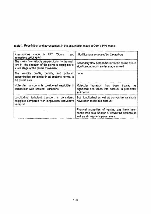
Tablel. Redefinition and advancement in the assumption made in Oom's PPT model

j~ssumptions made in PPT (Ooms and I Modifications proposed by the authors

The velocity profile, density, and pollutant 1 none I concentration are similar in all sections normal to

cowrokers, 1972 1974) The mean flow velocity perpendicular to the main flow in the direction of the plume is negligible till a late stage of the plume movement

Secondary flow perpendicular to the plume axis is sign~ficant at much earlier stage as well

1 Longitudinal turbulent transport is considered Both longitudinal as well as convective transports 1 negligible compared with longitudinal convective have been taken into account

the plume axis

Molecular transports is considered negligible in i comparison with turbulent transports I

Molecular transport has been treated as significant and taken into account in parameter estimation I

- Physical properties of venting gas have been considered as a function of downwind distance as well as atmospheric parameters

Table 2. The study setting

Effective plume height

The effective plume height is the height reached by the plume from the point of its exit from a stack/vent valve. The calculation of effective plume height assumes (as shown in Figure 1) that there is a virtual source of the plume at point A which is at a distance x, upwind from the transition point B. This assumption allows for the mixing effect of the jet. The distance x, is that which would be necessary to achieve the same concentration at the transition point if the mixing were done by the wind (Lees,1996). Then the rise of the plume is given as:

Subsequently maximum rise of the plume is estimated as:

Wliere, x,, = K8*w f x, and Kg = 200.0; (Cude,1974), and ( 5 )

The half angle of a plume (+) from a stack is generally 5' or 6' so that tang = 1. The drag coefficient Dc, as estimated by Cude (1974), is 0.4.

S ~ n c e length of the jet is inversely proportional to the root of momentum flux, the transition heights of the jet in still air conditions, lrr and in windy conditions, ltw are related as:

Finally the maximum effective rise of the plume is estimated using the following equation,

Briggs (1984) and Hanna et a1 (1982) have further modified the equations of maximum and effective nsc of the plume taking the temperature of venting gas into consideration. They have proposed equations:

Where, stability is defined as, sta = giT(dT/dy+R), (12)

'I'hc oulcome of all these equations with the modification of Briggs (1984) and Hanna et al. (1982) llavc been validated with experimental data for a range of distance 5 to 3,000 meter (Khan and Abbasi,l997a;

Figure 1, Illustrative figure showing coordinates of the plume as influnced by hot air injection

1997b). The results match well in the distance range 15 to 2,500 meter for the gases having efrcctive density of plume higher than air at exit point.

SIMULATIONS: FLAMMABLE GASES

Ethylene

Ethylene is a highly flammable gas which is stored under high pressure (above saturation pressure). Building of further pressure in the storage unit may cause release of gas through vent valve forming a jet which may subsequently take the shape of a plume (Table 3). The profile of various plume parameters (plume width, plume velocity, and gas concentration, in the plume) as estimated by the model are plotted in Figure 2. It reveals that the value of the parameters change sharply in the in~tial downwind travel of the plume: the velocity increases, the concentration of the gas in the plume decreases and the plume width increases. Subsequently extent of change decreases. This happens because at the initial stage of travel of the plume, turbulence (eddies) are generated which causes rapid entrainment of air in the plume. Subsequently a layer is developed around the edges ofthe plume wh~ch suppresses further entrainment of air and hence slows down the rate of dilution. Eventhough at the initial stage the effective density of the plume is higher-than-air, it disperses swiftly. It is due to highly energized release (with a venting velocity of 45.10 d s ) which imparts momentum to air and causes fast entrainment of air. The lower flammable concentration (LFC) for ethylene has been observed at around -385 m from the release point. The plume width at this distance is -1.28 m. The flammable concentration occurs high above the ground level (around 10.45 meters).

Propylene

Propylene is another flammable gas mostly stored in large quantities under pressure. A continuous release of gas through vent valve/pressure relief valve about 7 m above the ground forms a plume. The behavior of plume variables reveals that the dispersion of propylene is sluggish compared lo etliyle~ic (Table 3). It is because the effective density of the propylene plume is higher than ethylene. Tlic llamniable zone has been observed over an area of 415 m radius from the release point. The release and tl~spcrsion ofpropylene poses considerable hazards as the flammable zone envelops a large arca lhnl is also close to the ground level (-7.45 meters).

Isobutylene

lsobutylene is a flammable gas stored in lesser quantities compared to ethylene and propylene. Release of vapors (gas with aerosol) through vent valve would form a plume of density higher than air, wh~ctl would subsequently get diluted by entrainment of air. The behavior of dispersion parameters (Table 3) reveals a very slow dilution rate and hence building of flammable concentration over a large area. I t 1s bccausc:

i) a comparatively low venting speed would favor gravity-dominant dispersion due to the high density ofthe plume.

~ i ) relatively high density would favor formation of suppression layer around the plume edges which would inhibit cnlrainment of air and hence dilution.

Naturnl gas

Natural gas is a mixture of light flammable gases (such as methane and cthane) which is storcd a1 saturation pressure. Release of natural gas through a narrow opening would form a plume (-12 meters above the ground level). The results of the niodel output for this gas show a relatively fast dispersion compared to propylene and isobutylene. The lower limit of flammable concentration would be observcd

Table 3. Model output concerning dispersion of the gases

Chlorine I maximum plume rise = 9.56 rn I olume concentration 10 * kalm' 1 5.09 1 4.12 1 3.32 1 2.96 1 2.54

Chemicals

I olume width. m 1 0.512 1 0.644 1 0.714 / 0.864 1 0.944 1

@ Concentration estimated at the plume axis X Concentration estimated at the edge of the plume

Parameter Distance along down wind direction, meters

0 500 1,000 1,500 2,000 2,500 3.000

Dtstance, meters

+ veloc~ty*E-01 + concentrat~on * w ~ d t h

Figure 2. Illustrative figure showing variation of plume width and plume velocity with distnace of travel (for ethylene)

at a dislancc -90 m from point of release (at around 12.45 m above the ground level). It is becausc tlic effective density of this plume is low and the venting velocity is suficiently high, allowing rapid entrainment of air, consequently swift dilution.

SIMULATIONS: TOXIC GASES

Of the two toxic heavier-than-air gases studied here, chlorine (C12) has the slowest rate of dispersion. Othenvise the trend observed with chlorine is similar to the trends seen with the other five gases. For any given distance, the rate of change in concentration and plume velocity as well as plume width are lower compared to the other toxic gas ammonia (Table 3). As chlorine is the most toxic of the gases studied here and is also the most sluggish to disperse, lethal concentrations of this gas would easily build-up over large areas and persist for long durations.

Ammonia

Animonia is stored and processed in liquid state under refrigerated or pressurized conditions, Wlicr~ released, it forms an aerosol of ammonia liquid canied away as droplets along with ammonia vapor. As such ammonia gas has density (0.778 kg&) lower-than-air but due to aerosol formation the effective dcnsity of the plume (released vapors with aerosol) becomes higher than air. Hence the dispersion of ammonia is generally treated as if it were a heavy gas.

'I'he niodel output shows that ammonia disperses in a manner similar to chlorine but the trend is much more steep. The variations in plume width and plume velocity with distance are higher compared to C12. It is because droplets of ammonia liquid settle faster due to gravity leading to the formation of gradient for mixing, subsequently facilitating dilution. At the initial stage of release the effective density of the plume is 3 times higher than air but by the time it travels 375 meters, the density drops to 21% of the lnit~al value. The lethal concentration of the gas at the plume edge extends up to -645 m downwind at about 9.3 1 m above the ground.

IMPACT O F HOT AIR INJECTION : FLAMMABLE CASES

In order to contain the damage, if these hazardous gases get released (accidentally, or voluntarily to control bigger accidents such as explosions), we havc studied the option of increasing the release vclocity by injecting hot air as a possible means of diluting the gases and facilitate their dispersion. Such an act has the following consequences:

a ) hot inert air makes the released gas move higher and faster from the exit point; the effective relcasc velocity is a combination oftlie velocities of hot inert air and the hazardous gas;

b) turbulence is generated which effects the density of the plume as well as its momentum distribution:

C ) the high temperature of the air jet further disturbs the momentum balance by energizing the gas; however the air temperature should not be so high that it sparks a fire;

d ) thorough mixing takes place at the maximum height ofjet and along the downwind direction.

Wc have assumcd that thc shapc of thc plume would not bc disturbcd substantinlly. We havc czlrricd

o ~ ~ t sinIulations witliin the premises mcntioned above, assuming that the atmospheric stability conditions would re~nain the same throughout the dispersion process The impact of I%, 5% 7% Is%, and 20% increase in tlie effective jet velocity (i.e a conibination of the pas and the hot air jet velocities)

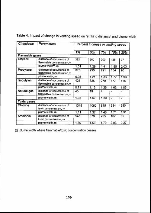
Table 4. Impact of change in venting speed on 'striking distance' and plume width

Chemicals

I toxic concentration, rn I plume width, m 1 1.39 1 1.63 1 1.79 1 2.03 1 2.27

Ammonia

@ plume width where flammableltoxic concentration ceases

Parameters Percent increase in venting speed

toxic concentration, rn plume width, rn dlstance of occurrence of

1.11 545

1.37 378

1.46 235

1.71 107

1.91 65

A i C ,p2- . . . . . . . - ta L -

. . . . . . . . . . . . . . . . . . . . . . . . . . . . . . . . . . . . . . . . . . . . . . . . . . " '

c 8

0 1 I 1 I

1 3 5 7 9 11 13 15 17 19 21

Percent increase in venting speed, (%)

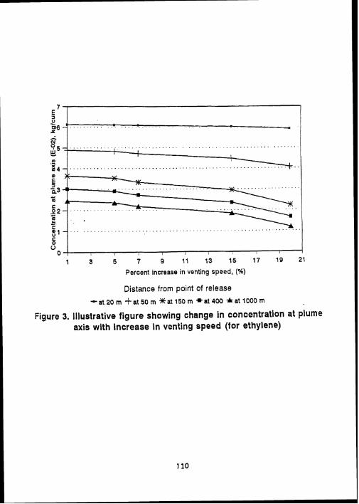
Distance from point of release *a t20 m $a150rn *at 150m +at400 *at 1OOOm

Figure 3. Illustrative figure showing change in concentration at plume axis with increase in venting speed (for ethylene)

0 1 3 5 7 9 11 13 15 17 19 21

Percent increase in venting speed,.

Distance from release point

" a t 2 0 m t a t 5 0 m *at 150 rn *a t400 m *at 1000 rn

Figure 4. Illustrative figure showing change in plume width increase in venting speed (for ethylene)

a) a comparatively lower effective density of ammonia, b) greater impact of hot air injection on the effective density of the plume and momentum

distribution.

CONCLUSION

We have presented empirical equations developed by us on the basis of Modified Plume Path Theory (MPPT) reported earlier by us. The MPPT, which was duly validated by us, enables one to study the dispersion ofheavier-than-air, lighter-than-air, and light-as-air gases. It is especially useful in assessing the risks posed by accidental release of hazardous gases.

The empirical equations dcscribed in this paper have been applied to possible accidental release of six hazardous gases from their storage vessels. It is seen that isobutylene release is the most hazardous as it would result in the formalion of a flammable cloud covering a large distance downwind.

The effects of decreasing the concentration and increasing the exiting velocity of the gases by injecting hot inert air at the point of exit were simulated. The studies reveal that a) the plumes of hazardous gases can be raised higher (thereby reducing the probability of they catching fire); b) the rate of dilution of the hazardous gases in the plume can be made faster; and c) the 'distance of impact' (in other words 'striking distance') can be significantly reduced, by hot air injection. For exanlple, an increase of 20% ill venting speed ofisobutylene by hot air injection raises the plume edge to an additional above ground and rcduccs its 'striking distance' by -370 m. Similarly an increase in the venting speed of chlorinc by 20% increases the plume height by 0.9Sm and reduces the range of lethal loxic concentration build-up by -1 100 m.

ACKNOWLEDGMENT

Authors are thankful to All India Council of Technical Education (AICTE) for sponsoring "Unit for Computer Aided Environmental Managcrnent (CAEM)" which made possible this study.

LIST OF SYMBOLS

local characteristics width, m concentration of gas on the plume axis, kgim3 distance along the plume axis from the release point to a certain point, rn temperature of the plume at any point inside the plume, K plume velocity on the plume axis in the direction of the tangent to the plume axis, mis venting speed, mis density of air, kgimJ effective density of plumeljet, kgim' dimensional number vertical distance above transition point, m maximum rise of plume, rn effective rise of plume, m lateral distance where maximum rise of plume occur, m lateral distance along down wind direction, m lateral distance from virtual source to transition point, m w~nd velocity, mls volunlctric flow rate of gas, m?s gravitational acceleration , mis2

drag coefficient transition height in still air, m transition height in windy conditions, m total effective height reached by the plume, m height of the vent, m momentum flux at exit point dry adiabatic laps rate, 'Clm vertical distance, m half angle of the plume from the stack

REFERENCES

1 . Briggs, G A, Plunre rise by buoyancy e f i c t s , Atmospheric science and power production, 1984 , p.327.

2. Contini, S, Amendola, A, and Ziomas, I, Benchmark exercise on major hazard analysis, Conrmissron of the Europearr Commu~irties, Joint Research Centre. ISPRA, Itlay, 1991, p2.

3 . Cude, A L,. Dispersion of gases related to atmosphere from reliefvalves, ChemicalEnninecr, 1974, 2!U, P 629.

4. Hanna, S R, Briggs, G A, and Hosker, R P,. Handbook on atmospheric diffusion, Keporr DOE-TIC 11223 Am~os . lurbulence anddrfusion lab, Dept, of Energy, Washington, D.C., 1982.

5 . Khan, F I, and Abbasi, S A, Modelling of dispersion of heavy gas based on modification in Plume Path Theory, Atmos fin press), 1997a,

6. Khan, F I , and Abbasi, S A, "Application of the recently modified PPT on the dispersion of sonic heavy gases", lOrh regional IUAPPA cotference, Gumu, Ssuyu, Istanbul, Turkey, 23-26 September. 1997b

7. Lees, F P, Lossprever~lion irr process industries, Buttenvorths, London, 1996

8. Ooms, G, A new method for the calculations of the plume path of gases emitted by stack, 1972, L, p 899.

9. Ooms, G, and Mahiue, A P. The plume path of vent gases, Losspreverrtiorr and safely pro~noriotr rrr process i~rdttsrries, Elsevier, New York, 1974.

10. Ooms, G, Mahiue, A P, and Zelis, F. The plume path theory of vent gases heavier than air, Proceeditrg oflhejirsr Inrcrr~a~ior~al loss prevetrrion synlposiunr, Delfl, The Nctherlands, 2-3 May, 1974.

11. Ooms, G an Duijm, N J, Dispersion of stack plumc heavier than air, Armospheric dispersion o j heavy gases atrd snrallpurt~cluates s)Inrposrum, Delft, The Netherlands, 1983

Chapter 8

APPLlCATlONS OF THE RECENTLY MODIFIED PLUME PATH THEORY ON THE DISPERSION OF SOME HEA W GASES'

Dispersion of several common 'heavy' gases (sulphur dioxide, ammonia, hydrogen sulphide, and chlorine) has been modelled on the basis of modifications in plume path theory recently done by us (Khan and Abbasi, 1997). The model takes Into account, among other things, the variations in temperature, density, and specific heat during the movement of the heavy gas plume. Studies have also been carried out to simulate the effects of wind speed, density of gas, and venting speed on the plume dispersion. Based on the simulations a set of empirical equations have been developed. The equations have been validated by theoretical as well as experimental studies.

Release rate is found to be one of the most important parameter which dictate plume behaviour and geometry.

Key words : gaseous dispersion, heavy gases, plume path theory, industrial hazards

INTRODUCTION

Plume path theory (PPT) was proposed by Ooms (1972) and has been used mainly to calculate the plume path of lighter-than-air and light-as-air gases escaping from stacks into the atmosphere at atmospheric temperature and pressure. Later this theory was extended

' Presented in Symposium on Air Qualiry Managemenl al Urban, Regional and Global Scales, 23-26 September, 1997, Istanbul, Turkey, (kindly see page A2)

to 'heavy' gases (of density higher than air; Ooms et a/. 1974) with a number of assumptions. .

Numerous applications of the PPT have been reported, for example, Rottman et a/.. (1985) and McQuaid (1986) have used the theory for analysing toxic gas dispersion; ~iewstadt (1992), Blewitt ef a/. (1987) and Weil (1988) have used the same for vapour doud modelling; and Ooms and Duijm (1983) have used it to estimate the dispersion of heavy gases coming out at high momentum from stacks. The theory has also been the basis of commercial packages PLUME and HFPLUME. But in-spite of the obvious potential of Ooms' theory, it has not enjoyed wider applicability because the main assumptions which had limited its applicability, have not yet been overcome. Recently these authors have modified Ooms's theory to significantly enhance its range, accuracy, and precision (Table 1). Most significantly we have enabled application of the theory to 'heavy gases' which is a much less explored domain of air quality modelling than dispersion of lighter- than-air or light-as-air gases. Based on simulations done with the help of model developed by us, we have evolved a few empirical relations to study the effect of atmospheric operating variables (wind velocity, venting speed, venting temperature, atmospheric temperature, etc.) over dispersion. These equations enable air pollution dispersion studies with less computational costs and greater accuracy.

MODIFIED PPT MATHEMATICAL MODEL

in the earlier form of PPT (Ooms and co-workers, 1972; 1974; 1983) only three parameters (u,p,c) have been considered as significant. In the present work temperature also has been taken as one of the dominant parameters. incorporating the aspects of plume density and temperature, and specific heat, the plume characteristics can be written as:

Where u(s,r,q),.p(s,r,+),c(s,r,+) represent the values of the variables at an arbitrary point in the plume; u ,r ,c denote the values of variables relative to the surroundings on the plume axis in the direction at a tangent to the plume axis (Figure 1).

Plume path

As the plume flows through the atmosphere, air is entrained. We have tried to represent the entrainment in terms of mass flow equations keeping the following facts in mind :

a) in the vicinity of vent or release point venting velocity is higher than wind velocity,

b) at a sufficiently long distance downwind, the velocity of the plume may equal the wind velocity,

C) atmospheric turbulence is one of the most effective factors causing entrainment

Mass flow equation

Figure I. The plume coordinates as used in the present study

The values of entrainment coefficient a,= 0.0762, a, = 0.61, and a,= 1.0 have been taken from Krogstad and Jacobsen (1991).

component Mass Balance :

The component mass balance over a cross section of plume is worked out as :

d( Icu2xrdr) 1 ds = 0 (6) This implies that no gas is assumed to be present in the atmosphere outside the plume.

Momentum Balance :

In plume, the momentum occurs mainly due to

a) entrainment of air,

b) force exerted by wind.

Keeping these in view the momentum balance in downwind direction can be written as :

d( ~(pu2cos~2nrdr))/ds=2xb8pa~a{a1~U'~+a2ua~sin~~cos~+a3u}+cdnbspau~~sin3q (7)

The momentum balance in the cross wind direction is a combination of

density spread,

e drag force exerted by wind.

The final balance equation can be written as :

Energy Balance :

The energy balance for the plume implies that the amount of heat emitted by the gas per unit time is conserved with respect to a chosen reference. So, for a reference temperature T,,, the energy balance equations can be written as:

If it is assumed that air and vent gas obey the ideal gas law, than the temperatures (plume and air temperature) can be expressed as

T = M,PI(Rp) and T, = M,P/(Rp,) (10)

Where, M, and M, represent molecular weights of plume (air and gas) and air respectively at any point in the plume. As molecular weight and specific heat differ, unlike what was assumed in the original PPT (Ooms, 1972), these variables can be expressed as:

M, = M,cT I (c,T,) + M,(l-cT/(coTo) (71)

cp = {M,cp,cT/(c,T,) + M,cp,(l-cT/(c,T,)} /M, (12)

Combining the above energy balance equations with molecular weight variation and specific heat variation, the final equation can be written as :

d( ~M,cpl(M,cp,) ' u[l -plp,,{l+ c*pd(c,p)(M,IM,,-1 )}12nrdr)lds = 2n*bl* (l-p~p,o){a,~u'~+a2'ualsincplc~scp~a~~~ (13)

SOLUTION OF THE MODEL and VALIDATION

BY substituting the similarity profile to these conservation equations, integrals can be calculated by a suitable numerical integration technique-here we have used Siphons-113 technique. Sets of non-linear simultaneous equations have been solved by using Newton- Raphson method coupled with L-U decomposition technique. The model has been solved for and different atmospheric operating conditions are presented in Table 2. The results of the models have been validated against experimental data (Khan and Abbasi, 1997). The comparison of the plume path (height of plume rise) obtained by our model with the results reported by Bodurtha (1961) and Moore et a/. (1988) and the experimental results (Khan and Abbasi, 1997) are presented in Figure 2. Good qualitative as well as quantitative agreements have been observed.

parametric effect

To generalise the effect of wind speed, density and venting speed on the plume path, we have developed some empirical equations. These equations directly predict the behaviour of plume variables ( gas concentration in plume, plume density, local plume width, plume velocity ) with other operating variables viz : density of gas, venting speed, etc.

For this purpose a dimensionless number Qf has been defined as:

af = UJU;(PJP)

A = -0.00395848*log(Qf) - 0.01925951

B = -0.1 6083 'log(Qf) + 0.091 579

u' = A'ln(s) + B

A = 0.159874 + 0.960923 ' Q, - 1.24869'~: + 0.3728 Q;

8 = -0.47832 + 0.0418951 *a f + 0.153298 ' Q: c*= A'ln(s) + B

A = -0.0161965 + 0.00543481 ' Qr0.00128631 ' QfZ 8 = 0.183894 ' exp(-0.382484 ' Qf )

b, = A*ln(s) + B

A = 0.0157719 + 0.104969 Qf - 0.0347085 ' Q:

8 = 0.953469 Q~~~~~~

T = A ' In@) + B

A = 3.67477 + 7.61097 Qf - 2.42655 Q:

= -8.5476 - 58.7278 ' Qf + 26.7875~:

The outcome of equations have been validated with experimental data for a range of dlstance ( 20 to 5,000 meters). The results match well in the distance range 50 to 3,500 meter.

Table 1. Redefinition and advancement in the assumption made in Oom's PPT model

Assumpfions made in PPT (Ooms and cowrokers,l972; 1974)

The mean flow velocity perpendicular to the main Row in the direction of the plume is negligible till a late stage of the plume movement

The velocity profile, density, and pollutant concentration are similar in all sections normal to the plume axis

Molecular transports is considered negligible in comparison with turbulent transports

Longitudinal turbulent transport is considered negligible compared with longitudinal convective transport -

-

Modifications proposed by the authors

Secondary flow perpendicular to the plume axis is significant at much earlier stage as well

none

Molecular transport has been treated as significant and taken into account in parameter estimation

Both longitudinal as well as convective transports have been taken into account

Physical properties of venting gas have been considered as a function of downwind distance as well as atmospheric parameters

. . . . . . . 30 . . . . . . . . . . . . . . . . . .

c - -- Moore et d. model a, f -20 ...... 8oaurlhr ",ddil.

Expmrimentml results

-30 - modifid PPT mod01 . . 1- -40 0 2 0 4 0 6 0 80 100

Figure 2. Comparison of plume path estimated by PPT with other models and experimental results

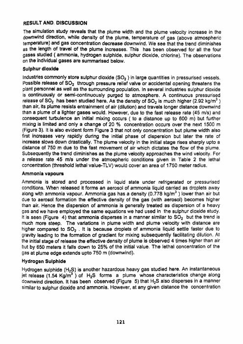
RESULT AND. DISCUSSION

The simulation study reveals that the plume width and the plume velocity increase in the downwind direction, while density of the plume, temperature of gas (above atmospheric tempemture) and gas concentration decrease downwind. We see that the trend diminishes as the length of travel of the plume increases. This has been observed for all the four gases studied ( ammonia, hydrogen sulphide, sulphur dioxide, chlorine). The observations on the individual gases are summarised below.

Sulphur dioxide

Industries commonly store sulphur dioxide (SO, ) in large quantities in pressurised vessels. Possible release of SO2 through pressure relief valve or accidental opening threatens the plant personnel as well as the surrounding population. In several industries sulphur dioxide is continuously or semi-continuously purged to atmosphere. A continuous pressurised release of SO2 has been studied here. As the density of SO2 is much higher (2.92 kglm3 ) than air, its plume resists entrainment of air (dilution) and travels longer distance downwind than a plume of a lighter gases would. However, due to the fast release rate (45 mls) and consequent turbulence an initial mixing occurs ( to a distance up to 600 m) but further mixing is limited and only a change of 20 % concentration occurs over the next 1500 m (Figure 3). It is also evident form Figure 3 that not only concentration but plume width also first increases very rapidly during the initial phase of dispersion but later the rate of increase slows down drastically. The plume velocity in the initial stage rises sharply upto a distance of 750 m due to the fast movement of air which dictates the flow of the plume. Subsequently the trend diminishes as the plume velocity approaches the wind velocity. For a release rate 45 m/s under the atmospheric conditions given in Table 2 the lethal concentration (threshold lethal value-TLV) would cover an area of 1750 meter radius.

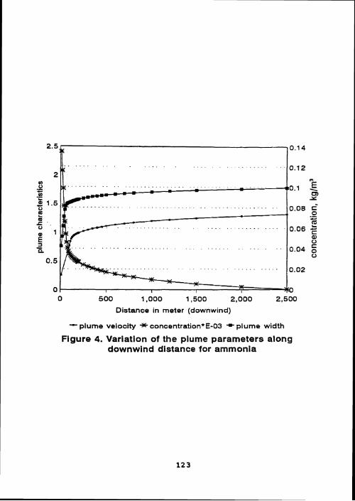
Ammonia vapours

Ammonia is stored and processed in liquid state under refrigerated or pressurised conditions. When released it forms an aerosol of ammonia liquid carried as droplets away along with ammonia vapour. Ammonia gas has a density (0.778 kg/m3 ) lower than air but due to aerosol formation the effective density of the gas (with aerosol) becomes higher than air. Hence the dispersion of ammonia is generally treated as dispersion of a heavy gas and we have employed the same equations we had used in the sulphur dioxide study. It is seen (Figure 4) that ammonia disperses in a manner similar to SO, but the trend is much more steep. The variations in plume width and plume velocity with distance are higher compared to SO2 . It is because droplets of ammonia liquid settle faster due to gravity leading to the forrnatlon of gradient for mixing subsequently facilitating dilution. At the initial stage of release the effective density of plume is observed 4 times higher than air but by 650 meters it falls down to 25% of the initial value. The lethal concentration of the gas at plume edge extends upto 750 m (downwind).

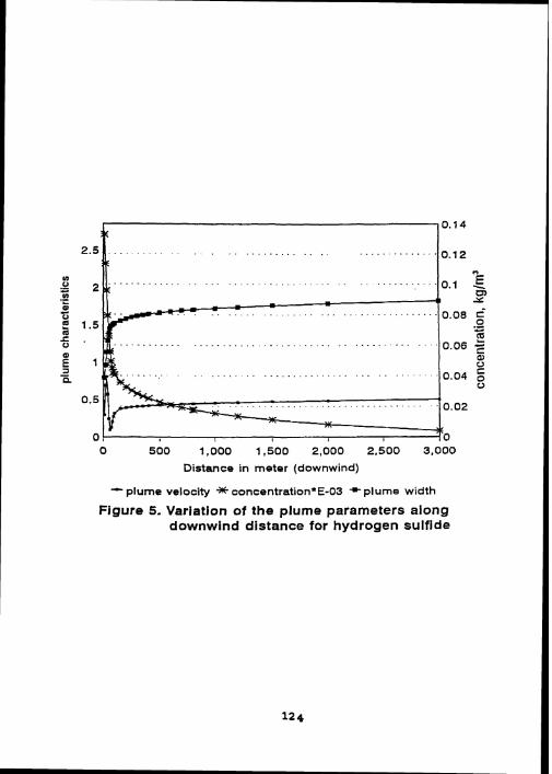
Hydrogen Sulphlde

Hydrogen sulphide (H2S) is another hazardous heavy gas studied here. An instantaneous jet release (1.54 ~ ~ / m ~ ) of H2S forms a plume whose characteristics change along downwind direction. It has been observed (Figure 5) that H,S also disperses in a manner similar to sulphur dioxide and ammonia. However, at any given distance the concentration

0 500 1,000 , 1,500 2.000 2,500 3,000

Distance in meter (downwind)

-plume velocity *concentration E-03 *plume width

Figure 3. Variation of the plume parameters along downwind distance for sulfur dioxide

0 500 1,000 1,500 2,000 2,500

Distance in meter (downwind)

' plume velocity * concentration'E-03 * plume width

Figure 4. Variation of the plume parameters along downwind distance for ammonia

0 500 1,000 1,500 2,000 2.500 3,000

Distance in meter (downwind)

-plume velocity * concentration*E-03 *plume width

Figure 5. Variation of the plume parameters along downwind distance for hydrogen sulfide

Table 2. Ambient operating variables used in the study

of H,S at the plume edge is higher compared to ammonia but lower compared to sulphur dioxide. It may be due to the following reasons :

i) the density effect is higher in case of H2S, resulting in greater resistance to mixing with air and hence dilution of the gas;

ii) a slower rate of release compared to ammonia reduces the initial turbulence and subsequently slows down the rate of dilution;

iii) a higher release rate as well as lower density effect makes H,S dispersion faster compared to SO, (all other conditions remaining the same).

The plume width and plume velocity also follow the same trend as observed for concentration.

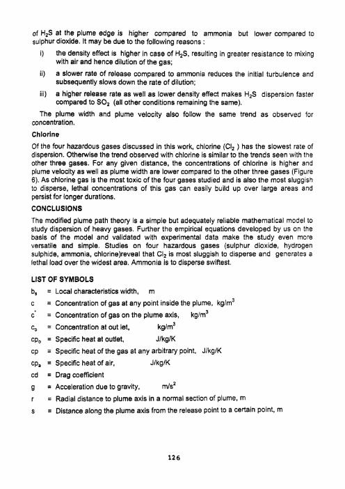
Chlorine

Of the four hazardous gases discussed in this work, chlorine (CI, ) has the slowest rate of dispersion. Otherwise the trend observed with chlorine is similar to the trends seen with the other three gases. For any given distance, the concentrations of chlorine is higher and plume velocity as well as plume width are lower compared to the other three gases (Figure 6). As chlorine gas is the most toxic of the four gases studied and is also the most sluggish to disperse, lethal concentrations of this gas can easily build up over large areas and persist for longer durations.

CONCLUSIONS

The modified plume path theory is a simple but adequately reliable mathematical model to study dispersion of heavy gases. Further the empirical equations developed by us on the basis of the model and validated with experimental data make the study even more versatile and simple. Studies on four hazardous gases (sulphur dioxide, hydrogen sulphide, ammonia, ch1orine)reveal that Ci, is most sluggish to disperse and generates a lethal load over the widest area. Ammonia is to disperse swiftest.

LIST OF SYMBOLS

b, = Local characteristics width, m

c = Concentration of gas at any point inside the plume, kglm3

c' = Concentration of gas on the plume axis, kglm3

c, = Concentration at out let, kglm3

cp, = Specific heat at outlet, JlkglK

cp = Specific heat of the gas at any arbitrary point, JlkglK

cp, = Specific heat of air, JIkgIK

cd = Drag coefficient

g = Acceleration due to gravity, mls2

r = Radial distance to plume axis in a normal section of plume, rn

s = Distance along the plume axis from the release point to a certain point, m

. . , . . . . . . . . . . . . . . . . . .

0 700 1400 21 00 2800 3500 4200 4900

Distance downwind, m

-plume velocity * conoentration*E-03 *plume width

Figure 6. Variation of the plume parameters along downwind distance for chlorine

M,~ = Molecular weight of plume at the exit of the gas (gas and air)

p = Absolute Pressure, kPa

pr = Prandtal number

T = Temperature of the plume at any point inside the plume, K

To = Temperature of the plume at the release point, K

T, = Temperature of the atmosphere, K

T,, = Temperature of the atmosphere at release point, K

u = Plume velocity at any point in the plume in the direction of the tangent to the plume axis, mls

u' = Plume velocity on the plume axis in the direction of the tangent to the plume axis, mls

u' = Entrainment velocity due to atmospheric turbulence, m/s

U, = Wind velocity, mls

u, = Venting speed, mls

p = Plume density at any point in the plume, kglm3

pa = Density of air, kg/m3

pa, = Density of air at release point, kg/m3

p, = Density of gas, kglm3

p* = Density difference between plume and atmosphere, kglm3

a, = Entrainment coefficient of a free jet

a, = Entrainment coefficient due to thermal stratification

a, = Entrainment coefficient due to atmospheric turbulence

. = Turbulent Schemedit number

4 = Angle between plume axis to horizontal component

d = Length of transition zone, m

Qf = Dimensional number

REFERENCES

1. Blewitt, D N, Yohn, J F, Koopman, R P, and Brown, T C, (1987). AlChE Int. Conf. on vapour cloud modelling, Boston. Massachusetts, New York.

2. Bodurtha, F T, (1961). The behaviour of dense stack gases, J. Air Pollution Contr. Asso.,l I, 431.

3. Khan, F I, and Abbasi, S A, (1997). Modelling of dispersion of heavy gas based on modification in Plume Path Theory, Atmos Environ., ( in press ).

Krogstad, P,A, and Jacobsen, cp. (1991) Dispersion of heavy gas (Air pollution control), Elsavier Publication, 63-678.

McQuaid, J, (1986). Refinement of estimates of consequence of toxic vapour release, Procd. IChmE Sym., Manchester.

Moore, G E, Milich, L B, and Liu, M K, (1988). Study on Plume behaviour using lidar and SF6 tracer at flat and heavy site, Atmos Environ., 22, 1673.

Niewstadt, F T M, (1992). A large -eddy simulation of a line source in a convective atmospheric boundary layer -11, Dynamic of a buoyant line source, Atmos Environ. 26 A, 499.

Ooms, G, (1972) . A new method for the calculations of the plume path of gases emitted by stack, Atmos Environ, . 6 , 899.

Ooms, G, and Mahiue, A P, (1974). The plume path of vent gases, Loss prevention and safety promotion in process industries, Elsevier New York USA

Ooms, G, Mahiue, A P, and Zelis, F, (1974). The plume path theory of vent gases heavier than air, Proceeding of the first International loss prevention symposium, Delft, The Netherlands

Ooms, G, and Duijm, N J, (1983). Dispersion of stack plume heavier than air, IUTAM Sym on Atmospheric Dispersion of Heavy Gases and Small particles, Delft, The Netherlands.

Rottman, J W, Simpson, J E, Hunt, J C R, and Bitter, R E, (1985). Hazardous Materials, 11, pp 325.

Weil, J C, (1988). Plume rise (Eds : Venkatram and Wyngaard) , Amer Metr Soci., Boston USA.

Chapter 9

HAZDlG : A NEW SOFTWARE PACKAGE FOR ASSESSING THE RISKS OF ACCIDENTAL RELEASE OF TOXIC CHEMICALS*

HAZDIG (HAZardous Dlspersion of Gases) is a user-friendly PC based software for generating scenarios for the emissions and gaseous dispersion of hazardous chemicals. It can simulate accidental as well as normal release but has been specifically developed as a tool for studying accidental release of hazardous chemicals and its consequences. HAZDIG is made-up of five main modules - data, release scenario generation, dispersion, characteristics estimation, and graphics.

HAZDIG incorporates latest models for estimating atmospheric stability (Van Ulden and Hostlag, 1985; Hsu, 1992; Erbink, 1995) and dispersion (Pasquill and Smith, 1983; Van Ulden, 1988; Erbink, 1993; Khan and Abbasi, 1997a). The data needed to run the models is easy to obtain and feed - properties of chemicals, operating conditions, ambient temperature, and a few commonly available meteorological parameters. A database containing various proportionality constants and complex empirical data has been built into the system. The graphics module enhances the user friendliness of the soware, and enables presentation of the results in an easy- to-understand and visually appealing manner. The output of the software is so fomaffed that it can be directly used for reporting the results without the need of editing.

' Accepted for publication in Journal ofLoss Prevention in Process Industries, U K (kindly see page A 3 )

130

Key words : Consequence analysis, dispersion of gases, industrial accidents, hazard assessment

INTRODUCTION

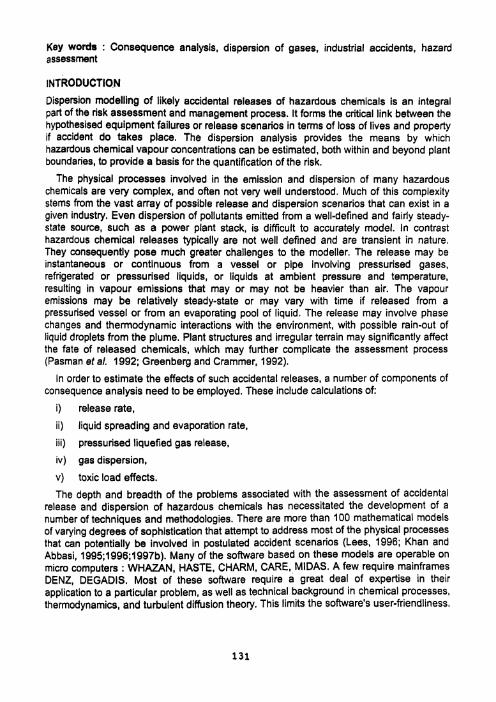
Dispersion modelling of likely accidental releases of hazardous chemicals is an integral part of the risk assessment and management process. It forms the critical link between the hypothesised equipment failures or release scenarios in terms of loss of lives and property if accident do takes place. The dispersion analysis provides the means by which hazardous chemical vapour concentrations can be estimated, both within and beyond plant boundaries, to provide a basis for the quantification of the risk.

The physical processes involved in the emission and dispersion of many hazardous chemicals are very complex, and often not very well understood. Much of this complexity stems from the vast array of possible release and dispersion scenarios that can exist in a given industry. Even dispersion of pollutants emitted from a well-defined and fairly steady- state source, such as a power plant stack, is difficult to accurately model. In contrast hazardous chemical releases typically are not well defined and are transient in nature. They consequently pose much greater challenges to the modeller. The release may be instantaneous or continuous from a vessel or pipe involving pressurised gases, refrigerated or pressurised liquids, or liquids at ambient pressure and temperature, resulting in vapour emissions that may or may not be heavier than air. The vapour emissions may be relatively steady-state or may vary with time if released from a pressurised vessel or from an evaporating pool of liquid. The release may involve phase changes and thermodynamic interactions with the environment, with possible rain-out of liquid droplets from the plume. Plant structures and irregular terrain may significantly affect the fate of released chemicals, which may further complicate the assessment process (Pasman eta/. 1992; Greenberg and Crammer. 1992).

In order to estimate the effects of such accidental releases, a number of components of consequence analysis need to be employed. These include calculations of:

i) release rate,

ii) liquid spreading and evaporation rate,

iii) pressurised liquefied gas release,

iv) gas dispersion.

v) toxic load effects.

The depth and breadth of the problems associated with the assessment of accidental release and dispersion of hazardous chemicals has necessitated the development of a number of techniques and methodologies. There are more than 100 mathematical models of varying degrees of sophistication that attempt to address most of the physical processes that can potentially be involved in postulated accident scenarios (Lees, 1996; Khan and Abbasi, 1995;1996;1997b). Many of the software based on these models are operable on micro computers : WHAZAN, HASTE, CHARM, CARE, MIDAS. A few require mainframes DENZ, DEGADIS. Most of these software require a great deal of expertise in their application to a particular problem, as well as technical background in chemical processes, thermodynamics, and turbulent diffusion theory. This limits the software's user-friendliness.

Moreover most of these software are unable to handle such accidental release situations as emissions of large quantities of chemicals with great force which may effect the existing atmospheric conditions.

In this context these authors have developed a software package capable of performing consequence analysis of normal as well as accidental release of chemicals. The package can handle myriad factors effecting the dispersion : density (lighter-thanllighter-aslheavier- than-air), convection, buoyancy and momentum. The main objectives behind the development of this software are:

a) wider applicability- HAZDIG incorporates larger number of models than existing packages dealing with accident simulation, to handle larger variety of situations with minimum data inputs.

b) greater sophistication- HAZDIG incorporates more precise, accurate, and recent models than handled by existing packages;

c) greater user-friendliness - HAZDIG is easier to run, and has a comprehensive database built into it.

ALGORITHM AND STRUCTURE OF HAZDIG

In essence, HAZDIG is a tool for consequence analysis, and performs assessment of likely consequences if an accident involving release of chemical occurs. The consequences are quantified in terms of damage radii or the radii of the area which shall be most susceptible to damage. HAZDIG computes likely impacts in terms of direct physical damage (shattering of window panes, caving of buildings) deaths due to blast wave injuries as well as toxic effects (chroniclacute toxicity, mortality). HAZDIG makes use of a wide variety of mathematical models (Table 1). For example, source models are used to predict the rate of release of hazardous materials, the degree of flashing, and the rate of evaporation. The impact intensity models are used to predict human response to different levels of exposures to toxic chemicals. HAZDIG handles several types of release and dispersion scenarios: liquid release, vapour release, gas release, two phase release, dispersion of lighter-than-air gases, buoyant dispersion, non-buoyant dispersion, and momentum driven dispersion. A special feature of HAZDIG is that it is able to handle dispersion of heavy (heavier-than-air) gases, and momentum driven dispersion with minimal input of data.

HAZDIG has been developed in object-oriented architecture using C++ as a coding tool. The software is compatible with DOS as well as WINDOWS operating environments. It is operable on computers with a minimum of 8 MB RAM and 80 MB ROM. The algorithm of HAZDIG is shown in Figure 1.

Details of the HAZDIG Modules

As seen in Figure 2 , HAZDIG consists of five main modules (Set of objects): data, release scenario generation, dispersion, characteristics estimation and graphics interface. Each module consists of two to three sub-modules (objects). These sub-modules depend on their parent modules as well as on other modules. A schematic diagram showing flow of information and dependency of different sub-modules to the main modules is presented in Figure 2.

I Estiutr concmtnatiun at study point I

Figure 1. Algoritlm of WIG

Figm 2, Hierarchical structum and nsssage flw sepuence ot WIG

:dl. 1, 113t o! varrous models rn-built m X A Z D I ~

- Model Incorpora tcd References

,-3-:inuo~5 -crmal flow through orlface Co~llson and R~chardron, 1911; Pllb~rough, 1999 rrfrrperatcd flow and heat transfe: model Clancey, 1974; 2:akc and Reid, 19l5; Drlvas, ? Y E : c~rerneated t h e r m o d ~ n u ~ c and f i3k mooe: Kletz. 1984; Leu:; and Eosteln, 1990

. " l : d i : O n e O Y S . .

-.>rmal rupture of YCSSI~ moael Hers e t al., 19':; Lees, 1996; Reed and Ciarh, 1383 :i!:lgerbtcd heat tidnsfer and evaporatraa Clancey. 1914. Faster. 1981: Hoodward and Mudan, :3Li

model s-perheared thennodynmc and evaporation Klerz, 1984. P~;srd snd Birhnol, 1988

model Greenbook, 1992; Shav and Brlrco, 1976 :as.ous r.1.a..

: ~ ~ c l n c l n e o ~ s thernadynarmc model COX and Comer, :9S>;Drrvas et al.,l983;Nolan e: d l . , 15 )C i~.::os:vely bolllng l~quid expbnung Pruqh, 1991: Kayes, 1986: Klerz, 1934

vapor explos10n vernart e: 2 1 . . 3 9 3 .:ntlnYoUS

5 - 0 sonic fluid d y n m c model Gr~enbook, 1932; see^, 1996; W~oaward, 1990 s m i c fluid dyndm~c model Covllson and Rlcaardson. 1917: Woodward an@ Nudan. 1991

:ro phase r.1.a..

:-frigeraced rhermodynarmc and heat- Fauskc,l964;198E:Feuske e t a ! . , 1984:Haque a n t Pepe, i 5 E O transfer model Kern, 1985, Derrg e t r ! . , 1934; Ksyes, !986

r .ae:heated thermodynuuc and hcar- Greenbook, 1992: Surripathala et d i . , 1330 tranllfc: model Perry er a l . , 1594: Lcung, 1990

;maeph.rrc boundary layer and macro- van Ulden and Ho:'.alag. 1985. Hnu, !932 S:ablllty mete3rologrcal parameters Erbink, 1995

based models :ISPERSTON

:.;:: r a s dlspsrrlon Parquill. Glfford m d - pa~qu111 and Srctt, 1983: Gitford, 1961 turner model TYIneT, 197031935 Robert model Robert e: a l . . 2492; Erbrnk, ;933 Sutton model Sutton, 1948,

'-5))' gas dl5peislon BOX. PLUME van Ulden, 1974;1988; Deaves. 1992 and SLAB model Khan and Rbbari, 19476; Predlkanls er dl., 1994

Earmak and Chan. :936;1388 .:: d l s p e r s ~ o n Jet release and dlrperrion Mahleb and Oames, 1974: Brown et a l . , 1393

model Khan and nbba3l. 1997a; Lees. 1996

-... l n l o u s re l ease Plume model

- 's tentaneous re l ease Puff model

3mc1 ISTI~UTION

.-:a:lnuous and Probit model -.Z:dntdneOYS

Mahleu and oomes, 1974; Lees, 1996 ~ h a n end libbes~, i991a; ooms and Tennekta. 1984 Greenberg and Cramer, 1992; Deaves, 1992 oomr and Tennekes, 1934; Van Ulden, 1992

ESSlenberg e t a : . , 1975; Greenbook. 1932 Clancey, 1917; Pietersen, 1993; CCPS, 1989

DATA module

m e main purpose of this module is to collect all relevant informations needed for the execution of other modules. The module consists of three main sub-modules derived from the main DATA module : release, dispersion and characteristics, and site specific. The dispersion and characteristic sub-module is further divided into sub-modules such as, lighter gas, heavy gas and momentum driven dispersion. The release sub-module bianches into instantaneous, continuous, jet, and two-phase release.

Each sub-module needs a set of data necessary for the analysis of that particular option. This is illustrated in Table 2 which shows the data list related to a continuous release accident scenario. Most of the options require data pertaining to chemical p:operties, operating conditions, and release conditions besides synoptic meteorological data. To cater this need, the requisite data base has been built into the software.

Scenario generation module

in this module release scenarios are generated for the unit under study. It is a very important input for the subsequent steps, as the accuracy of the forecast of the type of accident is directly influenced by the realism of the release scenario. Consequently all the subsequent steps are also strongly influenced.

Each release scenario is basically a combination of different likely events that may occur in an industry. Such scenarios are generated based on the properties of chemicals handled by the industry, physical conditions under which reactions occur or nactantslproducts are stored, geometries and material strength of vessels and conduits, e:c. External factors such as site characteristics (topography, presence of trees, ponds, rivers in the vicinity, proximity to other industries or neighbourhoods etc.) and meteorological conditions are also considered. In the available software packages such as \:'HAZAN (Technica,l992), EFFECTS (TNO, 1991), RlSKlT (VTT, 1993), and SAVE (TNO. 1992), these aspects have been used to some extent. But the level of sophistication needs to be enhanced substantially by using advanced models of thermodynamics, heat t-ansfer, and fluid dynamics to generate more realistic release scenarios. Furthermore, the user-friendliness of these packages have some limitations as a result of which several real- Ire studies conducted on the basis of these packages seem to have major lacunae. This is il:astrated by the following example.

A multinational project involving 11 institutions was operated (Contini et a/. 1991) to study the accidental release and dispersion of ammonia from a pressurised tank. The tjams utilised commercially available packages CRUNCH, DEGADIS, DENZ, HEAVY- PLUME, RISKIT, WHAZAN, SAFETI, EFFECTS, and DECARA (Contini et a/. 1991).

One of the basic aims of this study was to evaluate the efficacies of these packages and to set a benchmark for studies to be conducted in future. A total of five different accident scenarios were generated using these packages. Among these, the most common and worst disastrous accident scenarios invoked by the packages are:

catastrophic failure of a pressurised storage tank,

release of ammonia through a large hole on the roof. The scenario relevant to toxic dispersion is the second one. The packages mentioned above modelled the

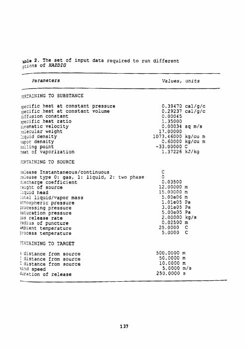
2. The set of input data required to run different ,,:ions of HAZDIG /

parameters Values, units

- .ER ;AINING T O S U B S T A N C E

ice~lfic heat at constant pressure ;jec;fic heat at constant volume ;:ifusion constant jaecific heat ratio ,:;nematic velocity -::ecular weight ; : j ~ i d density :iccr density :::ling point : s a t of vaporization

: 3 ? T A I N I N G T O S O U R C E

:.::ease Instantaneous/continuous C :elease type 0: gas, 1: liquid, 2: two phase 0 ::scnarge coefficient 0.03500 :e?cnt of source 12.00000 m ::$ld head 15.00000 rn :>:a! liquid/vapor mass 5.00e06 rn it-ospheric pressure l.Ole05 Pa ::>cessing pressure 3.01e05 Pa 5s:uration pressure 5.00e05 Pa ;as release rate 2.00000 kg/s : s d l u s of puncture 0.02500 m jrb~ent temperature 25.0000 C :recess temperature 5.0000 C

"3:AINING TO T A R G E T

"stance from source 500.0000 m . xstance from source 50.0000 m : alstance from source 10.0000 m , -*d speed 5.0000 m/s "Jrdtlon of release 250.0000 s -

second scenario as instantaneous two-phase release followed by denser-than-air- gas dispersion.

Table 3 presents a comparison of various models available with the different software used by the teems to study this scenario. It is seen that total of eleven different models are avabble in HAZDlG relevant to the study of the above mentioned problem, whereas MAXCRED (Khan and Abbasi, 1997c) has 6 models and other packages such as RlSKlT and SAFETI have only 4 models. Moreover, only HAZDIG generates the scenario of two- p h s e release followed by flashing, evaporation and dispersion (initially momentum driven dispanion with density effect) while others just identify two-phase release followed by dispersion (as non-buoyant puff).

We may mention here that we have recently developed a computer software package MAXCRED (Maximum Credible accident analysis) for rapid risk assessment. This software comprises of a Set of models to enable rapid study of damages likely to be caused if explosion, fire, or toxic release accidentally occur in a chemical industry (Khan and Abbasi, 1995;1996;1997b). MAXCRED has certain features, among others, for study of release patem and dispersion of chemicals (liquidlgases). HAZDIG, on the other hand, specialises in the study of toxic release and dispersion occurring as a consequence of accidents in chemical process industries. It incorporates much larger number and variety of models for this purpose than MAXCRED does. Its knowledge-base and out-put features are also substantially superior. In other words whereas MAXCRED is a general-purpose package for rapid risk assessment, HAZDIG is a specialised package devoted to toxic release occurring in industrial accidents.

We have also come across several other reports (NEERI, 1992; CISRA, 1993; TPL, 1993) in which the existing risk assessment packages have been used in studying accidental release of toxic chemicals. In all these reports several credible accident scenarios have been left unconsidered in a manner similar to the one illustrated in the multi-institutional study quoted by us above, indicating the lack of rigor andlor user- friendliness of the packages used.

The accident scenarios are generated based on chemical properties, operating conditions, and details of the processlstorage units. Once an accident scenario has been developed, it can be processed for further verification and consequence assessment. For the same unit and same operating conditions various plausible accident scenarios can be visualised. Thus, this option helps in simulating the various likely accidents, and characterising the worst plausible ones. The option handles six type of release scenarios; continuous liquid release, instantaneous liquid release, continuous gas release, instantaneous gas release, continuous two phase release and instantaneous two phase release. A data-base consisting of constants for different thermodynamic and fluid dynamic relations has been built-in with the option. This option uses advance thermodynamic (adiabaticlisotherrnal exoansion) and fluid dynamic (flow through orifice, uncompressed fluid. compressed fluid) 'models: The list of different models contained in the software is presented in Table 1. The architecture of this module is shown in Figure 3. The main release scenario module has three sub-modules, each consists of a set of functions to estimate different parameters. Brief descriptions of each of the sub-modules is presented below.

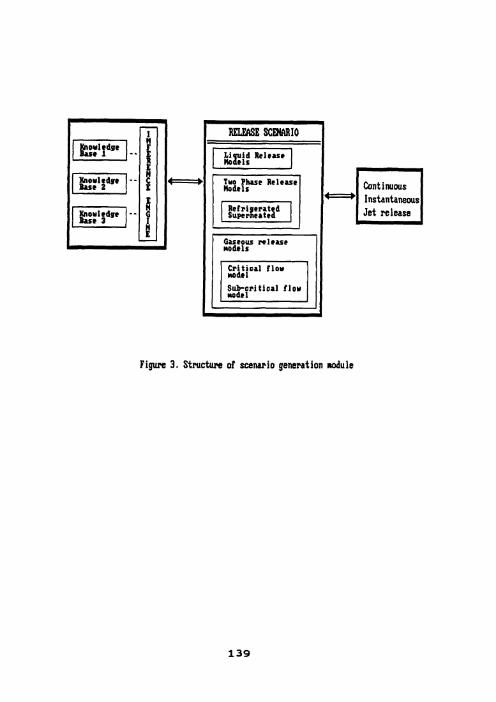
Jet release

models

Figure 3. Structure d scenmio generation d u l e

List Of models available with different software to study the and disperslon Of ammonia through a large hole in the roof of a tank

Remarks package for the study ofe study of catastrophic

1. Liquid out flow 2. Gas outflow 3. Two-phase outflow

IAN 4 . Evepotdtlon but not time independent

r: 1. Llquld out flow 2. Gas outflow 3. Two-phase outflow 4. Evaporation time dependent

1. Liquid outflow ~ : r 2, Gas outflow

3. Two-phase outflow 4. Heavy gas dispersion

1. Llquld outflow 2. Vapor outflow

k:s 3. Gas outflow 4. Two-phase outflow 5. Evaporation but not

tlme dependent

1. Liquid release 2. Gaseous release

C : ! 3. Tuo-phase release 4. Evaporatlon but not

time dependent 5. Light gas drsperslon 6. Heavy gas dispersion

1. Momentum release

Two phase release of amonla followed by the evaporation

3,4,6 and heavy gas disparslon.

2. Llquid release 3. Gaseous release 4. Two-phase release 5. Fiashlng of vapor 6. Evaporation but not 4,5,6,8,10

trme dependent 1 . Light gas dispersion 5. Heavy gar disparslon 9. Jet release and disoersien

10. Plume characteristics 11. Puff characteristics

Two-ohase release followed br fl&rng of vapor and subseq;enr evaporation of remaining l~quid ammonia followed by heavy gas dispersion and puff characterlstlcs estlmatlon.

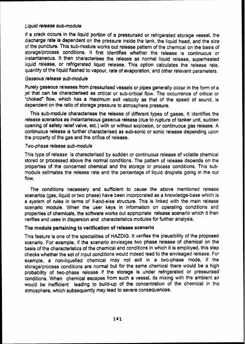
Liquid release sub-module

If a crack occurs in the liquid portion of a pressurised or refrigerated storage vessel, the discharge rate is dependent on the pressure inside the tank, the liquid head, and the size of the puncture. This sub-module works out release pattern of the chemical on the basis of storagelprocess conditions. It first identifies whether the release is continuous or instantaneous. It then characterises the release as normal liquid release, superheated iiquid release, or refrigerated liquid release. This option calculates the release rate, quantity of the liquid flashed to vapour, rate of evaporation, and other relevant parameters.

Gaseous release sub-module

Purely gaseous releases from pressurised vessels or pipes generally occur in the form of a jet that can be characterised as critical or sub-critical flow. The occurrence of critical or "choked" flow, which has a maximum exit velocity as that of the speed of sound, is dependent on the ratio of storage pressure to atmosphere pressure.

This sub-module characterises the release of different types of gases. It identifies the release scenarios as instantaneous gaseous release (due to rupture of tanker unit, sudden opening of safety relief valve, etc.) with or without explosion, or continuous gas release. A continuous release is further characterised as sub-sonic or sonic release depending upon the property of the gas and the orifice of release.

Two-phase release sub-module

This type of release is characterised by sudden or continuous release of volatile chemical stored or processed above the normal conditions. The pattern of release depends on the properties of the concerned chemical and the storage or process conditions. This sub- module estimates the release rate and the percentage of liquid droplets going in the out flow.

The conditions necessary and sufficient to cause the above mentioned release scenarios (gas, liquid or two phase) have been incorporated as a knowledge-base which is a system of rules in terms of if-and-else structure. This is linked with the main release scenario module. When the user keys in information on operating conditions and properties of chemicals, the software works out appropriate release scenario which it then verifies and uses in dispersion and characteristics modules for further analysis.

The module pertaining to verification of release scenario

This feature is one of the specialities of HAZDIG. It verifies the plausibility of the proposed scenario. For example, if the scenario envisages two phase release of chemical on the basis of the characteristics of the chemical and conditions in which it is employed, this step checks whether the set of input conditions would indeed lead to the envisaged release. For example, a non-liquefied chemical may not exit in a two-phase mode, if the storagelprocess conditions are normal but for the same chemical there would be a high probability of two-phase release if the storage is under refrigerated or pressurised. conditions. When chemical escapes from such a vessel, its mixing with the ambient air would be inefficient leading to build-up of the concentration of the chemical in the atmosphere, which subsequently may lead to severe consequences.

If HAZDlG finds that an envisaged scenario is not within the realms of probability, it modifies the scenario to the extent that it become plausible.

Dispersion module

This module consists of up-to-date mathematical models for simulating the accidents chosen as credible in the previous step. This module works out the dispersion characteristics profile, percentage of lethality, and damage radii of the release chemical. The output of this module quantifies impacts such as concentration at particular location, concentration profile, toxic dosage, damage radii of different impacts, and probabilities of causing lethality. The output of this object has been so formatted that it can be directly used in reports without having to do any editing. Moreover, using these results it is very easy to draw damagelrisk contours.

The mathematical models used in this module are listed in Table 1. Brief explanatory notes on the phenomena simulated by these models are presented below.

This module assesses the consequences of release and dispersion of toxic gaslvapour. it simulates different types of release scenarios such as; continuous release, two-phase release, and instantaneous release. In conducting dispersion studies it takes into consideration the densities of the gases or gas-air mixtures (because of the pronounced influence density exerts on the shape of the plume) and momentum of release. The models can thus simulate dispersions of heavier-than-air, lighter-as-air and lighter-than-air gaseslgas-air plumes. This module first estimates the concentration profile of the toxic gas that would develop consequent dispersion under the given meteorological conditions. It then works out the areas of toxic impact and the extents of toxicity that would be caused on the basis of exposure-based-toxicity data.

This module can handle the following options: heavy-gas dispersion, light-gas dispersion, momentum driven dispersion. The structure of this module is shown in Figure 4 and brief description of these options is presented below.

Option heavy-gas dispersion

This option estimates dispersions characteristics (concentration profile, distance travelled by the cloudlplume, and the dimensions of the cloudlplume) of the gases having effective density higher-than-air. It uses BOX model for instantaneous release (Van Ulden, 1974; Van Ulden and Hostage, 1985; Deaves, 1992; Erbink, 1993) and PLUME and SLAB model (heavy gas) for continuous release (Ermak and Chan , 1986;1988; Predikanis et a/. 1994; Langio and Schatzmawn, 1991; Khan and Abbasi, 1996) to estimate gas concentrations and other dispersion characteristics. The results are then passed on to damage estimation options to calculate the percent likelihood of lethality and area under influence for various degrees of toxicity.

Option lighcgas dispersion

In this similar operations are carried out for gases having density lighter-than-air orland lighter-as-air as in the previous option heavy-gas done for heavier-than-air gases. This option is in-built with various dispersion models: Gaussian model (instantaneous and continuous), Plume model (continuous), and Puff model (instantaneous) to estimate the dispersion characteristics for different release scenarios (Brington. 1985; Turner, 1970;1985; Robert et a/. 1992; Erbink, 1993) . The results are then used to estimate the

.-.---.-........ Elrurted S o m e ,

k!?? .* .'b"!!1 .In-built database

..A-..-..-...--

r ~ r t dirpcrrion 1

L.. -. -. - - . . . . . . -2

. I n - h i l t database

Figure 4 , Structure of dispersion aodule

toxic load (concentration) at particular location, chances of lethality at that location and radii of the areas under the influence of various degrees of toxicity. Probit models proposed by Clancey (1977), Pietersen (1990), and Greenbook (1992) are used for estimating lethality.

Option momentum-driven dispersion

As long as the momentum of the escaping gas is significant the density factor does not become operative but as soon as the momentum dies down to a level where the ambient air movements could effect dispersion, the density factors take over to influence the shape of the plume.

When the gas escapes at high velocity as from a jet or a vent, the momentum effect is more prominent and lasts longer (due to higher velocity of release) than when the release velocity (venting velocity) is low.

According to Lees (1996) releases in the form of jets can be of four types : (i) turbulent momentum jet in still air, (ii) buoyant plume in still air; (iii) plume dispersed by wind and (iv) jet-turbulent plume dispersed by wind. The behaviour of such jets and vents is as relevant to the intended discharges as to accidental discharges. The behaviour of the dispersion of such jets depends on the relative importance of discharge momentum, buoyancy effects, and of wind turbulence. We have used turbulent jet model along with plume dispersion, as in modified plume path theory to estimate this mode of dispersion.

Once the gas loses its momentum it is influenced by the density of the gas-air mixture relative to air. A difference in the molecular weight andlor in the temperature between the gas and the ambient air creates, in principle, such a density difference, but this density difference will affect the behaviour of the cloud only if the concentration of the gas is sufficiently high. A large proportion of the liquid droplets and a low air humidity favour the formation of a gas cloud heavier than air.

This type of release is generally observed in high velocity venting and relief of gases under high pressure through narrow passages, Initial buoyancy and high turbulence due to high jetting velocity are dominant factors for plume rise and dispersion. Khan and Abbasi (1997a), have proposed a model for jet dispersion of hazardous gases based on plume path theory. This option uses plume path theory (jet release) for analysis. The final output of this model is similar to the heavy-gas dispersion sub-module.

Characteristics estimation module

To estimate the characteristics of dispersion of gases due to an accidental release, the following accidental release conditions (with appropriate models) have been considered.

a) Gaseous release.

b) Liquid release at atmospheric pressure. This condition can further be categorised as: (i) liquid with a boiling point above ambient temperature which IS

processedlstored at a temperature below its normal boiling point: (ii) liquid with a boiling point below ambient temperature which is processedlstored at low temperature and atmospheric pressure.

c) Two phase release (liquid under pressure). This condition can also be further categorised in two classes: (i) liquid having normal boiling point above ambient

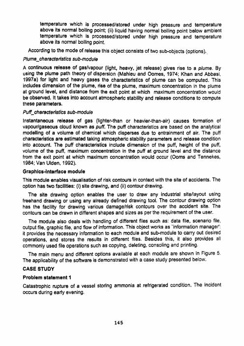
temperature which is processedlstored under high pressure and temperature above its normal boiling point; (ii) liquid having normal boiling point below ambient temperature which is processed/stored under high pressure and temperature above its normal boiling point.

According to the mode of release this object consists of two sub-objects (options).,

Plume-characteristics sub-module

A continuous release of gaslvapo~r (light, heavy, jet reiease) gives rise to a plume. By using the plume path theory of dispersion (Mahieu and Oomes, 1974; Khan and Abbasi, 1997a) for light and heavy gases the characteristics of plume can be computed. This includes dimension of the plume, rise of the plume, maximum concentration in the plume at ground level, and distance from the exit point at which maximum concentration would be observed. It takes into account atmospheric stability and reiease conditions to compute these parameters.

Puff-characteristics sub-module

Instantaneous release of gas (lighter-than or heavier-than-air) causes formation of vapourlgaseous cloud known as puff. The puff characteristics are based on the analytical modelling of a volume of chemical which disperses due to entrainment of air. The puff characteristics are estimated taking atmospheric stability parameters and reiease condition into account. The puff characteristics include dimension of the puff, height of the puff, volume of the puff, maximum concentration in the puff at ground level and the distance from the exit point at which maximum concentration would occur (Ooms and Tennekes, 1984: Van Uiden, 1992).

Graphics-interface module

This module enables visualisation of risk contours in context with the site of accidents. The option has two facilities: (i) site drawing, and (ii) contour drawing.

The site drawing option enables the user to draw any industrial sitellayout using freehand drawing or using any already defined drawing tool. The contour drawing option has the facility for drawing various damagelrisk contours over the accident site. The contours can be drawn in different shapes and sizes as per the requirement of the user.

The module also deals with handling of different files such as: data file, scenario file, output file, graphic file, and flow of information. This object works as 'information managet: it provides the necessary information to each module and sub-module to carry out desired operations, and stores the results in different files. Besides this, it also provides all commonly used file operations such as copying, deleting, consoling and printing.

The main menu and different options available at each module are shown in Figure 5. The applicability of the software is demonstrated with a case study presented below.

CASE STUDY

Problem statement 1

Catastrophic rupture of a vessel storing ammonia at refrigerated condition. The incident occurs during early evening.

* H A Z D I G lc) CPCE, Pondicherry.

I

I

I

I I

Figure 5. Main menu and available options in HAZDIG

Analysis

The problem has been identified as instantaneous release (boiling liquid expanding vapour explosion-BLEVE) of ammonia under slightly stable conditions (using macro meteorological data). Eventhough ammonia vapour has density lighter-than-air, light gas dispersion model can not be used because in the present case study, ammonia is stored in refrigerated condition and an instantaneous release (as BLEVE) would lead to the formation of vapour cloud consisting of liquid ammonia droplets. Thus the effective density of the cloud will be higher-than-air. HAZDIG also confirms this phenomenon and suggests two phase release with shock wave development and non-buoyant dispersion.

Table 4 shows the output of HAZDIG; it specifies accidental release scenario as- instantaneous two phase release of gas (flashing followed by evaporation) under sub- normal condition. It also presents the output of dispersion of heavy-gas module using BOX model. It suggests that at a distance of 500 meter from the accident site the concentration of gas would be 2.64E-06 kglm3, which is a lethal dose considering that STEL (short term exposure limit) lethality concentration 0.027.E-09 kg/m3 (Fowcetl and Wood, 1993). The concentration profile for ammonia with distance, shown in Figure 6, suggests that up to a distance of 1500 meters the concentration of ammonia would be above permissible limit vis a vis STEL (1 5 minutes exposure) for instantaneous exposure.

The puff characteristics of release and dispersion scenario can be interpreted from Table 4 which is an output of HAZDIG. It suggests that after 1 hour of release the puff would be around 250 meter in radius and about 10 meter high from the ground level. The maximum concentration of ammonia, 3.5'E-03 kg/m3, would occur at a distance of 5 meters from the release point. Figure 7 presents the damage contours of lethal dose over the area. It is clear that lethal concentration shall occur only within the industry's periphery (400 meter). However, high risk contour (representing 50% probability of lethality, estimated using probit function) would cover large area (1200 meter) which encompasses populated areas. Thus, the consequences due to release of toxic NH, have high risk (50% probability of lethality) to surrounding and for the populated areas near to the industrial site.

Problem Statement 2

Chlorine, stored under high pressure, is accidentally released from a storage vessel due to failure of flange in the forenoon in industrial area on a clear sun-lit day.

Analysis

We have defined the problem as continuous release of chlorine under unstable meteorological conditions. As chlorine is a 'heavy' (denser-than-air) gas and is released at high pressure (above vapour pressure) heavy-gas continuous model is used by HAZDIG to forecast the dispersion profile.

Table 5 presents the output of HAZDIG for chlorine release. It provides the accident release scenario as continuous two phase release of chlorine (flashing followed by evaporation) under pressurised condition. Table 5 also presents the output of heavy gas module using plume path model. It suggests that at a distance of 500 meter from industrial site the concentration of gas would be 5.409E-06 kglm3, which is above the lethal limit as per the STEL of 9 ,0~ -09 kg/m3. The concentration profile of chlorine with distance is

. . . . . . . . . . . . . . . . . . . . . . . . . . . . . . . . . . . . . . . . . . . . . . . . . . . .

1 , a , I , , m I ' " I " "

50 300 550 800 1,050 1,300 1,550 1,800 2,050

Downwind distance, rn

+ concentration STEL limit

Figure 6. concentration profile for the accidental release of ammonia

F~gure 7 . Risk contours for accidental release of ammonia; (A) represents severe rtsk contour, ( 8 ) high risk contour and (C) Low risk contour

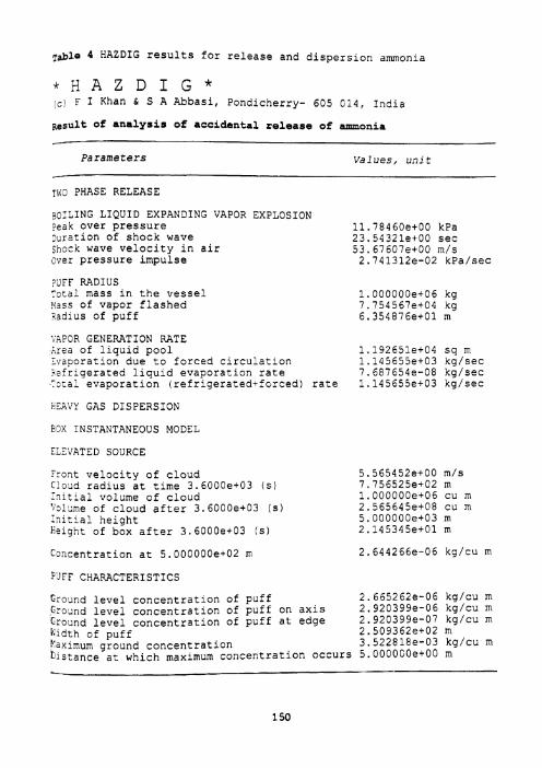
~ ~ b l e 4 HAZDIG results for release and dispersion ammonia

* H A Z D I G * ( c ! F I Khan & S A Abbasi, Pondicherry- 605 C14, India

Result of analysis of accidental release of ammonia

Parameters Values, unit

:WI PHASE RELEASE

EO:;ING LIQUID EXPANDING VAPOR 3XPL3SION ;eak over pressure 11.78460et00 kPa 2~ration of shock wave 23.54321et00 sec ;flock wave velocity in air 53.67607et00 m/s iver pressure impulse 2.741312e-02 kPa/sec

;gFF RADIUS :~tal mass in the vessel ~ 4 5 s of vapor flashed !adius of puff

'.'.??33 GENERATION RATE i r e a of liquid pool 1.192651et04 sq m S~aporation due to forced circulation 1.145655et03 kg/sec :efrigerated liquid evaporation rate 7.687654e-08 kg/sec

- + - :-LC; evaporation (refrigerated-fcrced) rate 1.145655et03 kg/sec

E3X INSTANTANEOUS MODEL

ELEVATED SOURCE

Frcnt velocity of cloud C!ocd radius at time 3.6000et03 ! s ) Initial volume of cloud :‘;?erne of cloud after 3.6000et03 (s) Znltial height Keigbt of box after 3.6000e+03 i s )

F7FF CHARACTERISTICS

Ground level concentration of puff 2.665262e-06 kg/cu m Groand level concentration of puff on axis 2.920399e-06 kg/cu m Ground level concentration of puff at edge 2.920399e-07 kg/cu m h!cth of puff 2.509362et02 m ~axirnum ground concentration 3.522818e-03 kg/cu m tlstance at which maximum concentration occurs 5.00@@6Oe+0@ m

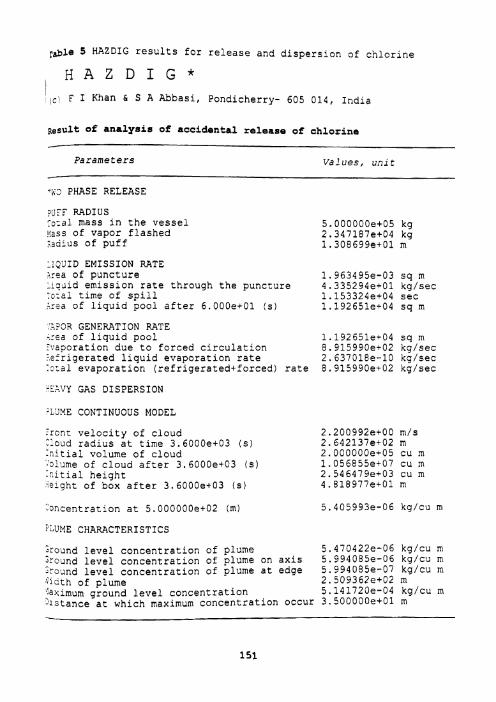
2 ~ 1 e 5 HAZDIG results for release and dispers~on of chlorine

H A Z D I G * ~ F I Khan & S A Abbasl, Pondlcherry- 605 014, Indla

uesult of analysis of accidental release of chlorine

Parameters Values, unit

+i(3 PHASE RELEASE

?3?? RADIUS :oral mass in the vessel 5.000000et05 gass of vapor flashed 2.347187et04 ;3i1~S of puff 1.308699et01

::,'>ID EMISSION RATE L r t a of puncture 1.963495e-03 ::?~iid emission rate through the puncrure 4.335294et01 . , . G ? time of spill 1.153324et04 ;:@a of liquid pool after 6.000e+01 (s) 1.192651e+04

';?3R GENERATION RATE ::$a of liquid pool 1.192651e+04 :,:~poration due to forced circulation 8.9i5990ei02 :efrigerated liquid evaporation rate 2.637318e-10 :::a1 evaporation (refrigeratedtforced) rate 8.915990et02

sq m kg/sec sec sq

sq m kg/sec kgisec kgisec

-5'IY GAS DISPERSION

'i3!4E CONTINUOUS MODEL

:rent velocity of cloud 2.200992e+00 m/s : :o~d radius at time 3.6000et03 (si 2.642137et02 m :?.ltial volume of cloud 2.OC0000e+05 cu m ;>lurne of cloud after 3.6000e+03 is) 1.056855et07 cu m ::ltlal height 2.546479et03 cu m :e:ght of box after 3.6000e+03 (s) 4.818977et01 m

:round level concentration of plume 5.470422e-06 kg/cu m !:oand level concentration of plume on axis 5.994085e-06 kg/cu m k ~ n d level concentration of plume at edge 5.994085e-07 kgicu rn :lath of plume 2.509362e+C2 m ;asimum ground level concentration 5.141720e-04 kg/cu m -lstance at which maximum concentration occur 3.500000e+01 m \

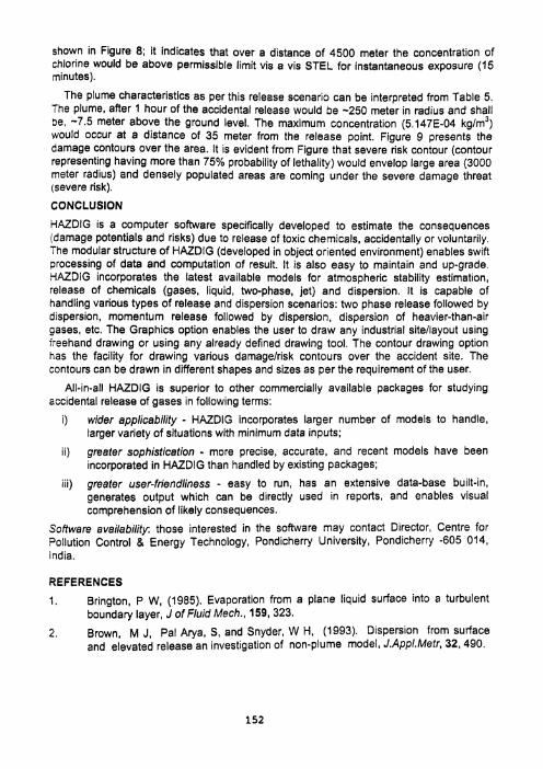
shown in Figure 8; it indicates that over a distance of 4500 meter the concentration of chlorine would be above permissible limit vis a vis STEL for instantaneous exposure (15 minutes).

The plume characteristics as per this release scenario can be interpreted from Table 5. The plume, after 1 hour of the accidental release would be -250 meter in radius and shall oe, -7.5 meter above the ground level. The maximum concentration (5.147E-04 kg/m3) would occur at a distance of 35 meter from the release point. Figure 9 presents the damage contours over the area. It is evident from Figure that severe risk contour (contour representing having more than 75% probability of lethality) would envelop large area (3000 meter radius) and densely populated areas are coming under the severe damage threat (severe risk).

CONCLUSION

HAZDIG is a computer software specifically developed to estimate the consequences (damage potentials and risks) due to release of toxic chemicals, accidentally or voluntarily. The modular structure of HAZDIG (developed in object oriented environment) enables swift processing of data and computation of result. It is also easy to maintain and up-grade. HAZDIG incorporates the latest available models for atmospheric stability estimation, release of chemicals (gases, liquid, two-phase, jet) and dispersion. It is capable of handling various types of release and dispersion scenarios: two phase release followed by dispersion, momentum release followed by dispersion, dispersion of heavier-than-air gases, etc. The Graphics option enables the user to draw any industrial sitellayout using freehand drawing or using any already defined drawing tool. The contour drawing option has the facility for drawing various damagelrisk contours over the accident site. The contours can be drawn in different shapes and sizes as per the requirement of the user.

All-in-all HAZDIG is superior to other commercially available packages for studying accidental release of gases in following terms:

i) wider applicability - HAZDIG incorporates larger number of models to handle, larger variety of situations with minimum data inputs:

ii) greater sophistication - more precise, accurate, and recent models have been incorporated in HAZDIG than handled by existing packages;

iii) greater user-friendliness - easy to run, has an extensive data-base built-in, generates output which can be directly used in reports, and enables visual comprehension of likely consequences.

Software availability: those interested in the software may contact Director, Centre for 'oilution Control & Energy Technology, Pondicherry University, Pondicherv -605 014, India.

REFERENCES

1. Brington, P W, (1985). Evaporation from a plane liquid surface into a turbulent boundary layer, J of Fluid Mech., 159, 323.

2. Brown, M J, Pal Arya, S, and Snyder, W H, (1993). Dispersion from surface and elevated release an investigation of non-plume model, J.Appl.Metr, 32, 490.

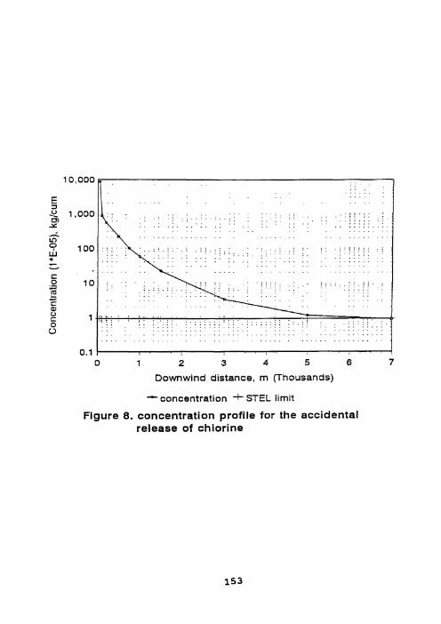
- concentration + STEL limit

Figure 8. concentration profile for the accidental release of chlorine

0.1

. . . . . . . . . . . . . . . . . , . . . . . . . . . . . i 0 1 2 3 4 5 6 7

Downwind distance, m (Thousands)

Figure 9. Risk contours for the accidental release of chlorine; (A) severe risk contour, and (B) high risk contour

CCPS (1989). Guidelines for chemical process quantitative risk analysis, Center for Chemical Process Safety, Publication number 0-8, AIChE, Washington, D C.

ClSRA (1993). Risk assessment of Chloralkali industry, Cell for Industrial Safety and Risk Analysis. CLRI, Madras, India.

Clancey, V J, (1974). The evaporation and dispersion of flammable liquid spillage's. Chemical Process Hazards, 5, 80.

Clancay, V J, (1977). Dangerous clouds, their growth and explosive properties, Chemical Process Hazards, 6,111.

Clancey, V J, (1974). The evaporation and dispersion of flammable liquid spillage's. Chemical Process Hazards, 5, 80.

Contini, C A, Amendal. A., and Ziomas, 1, (1991). Benchmark study on major hazard study, JRC-ISPRA, 134, Amestradam.

Coullson, J M, and Richardson, J F, (1977). Chemical Engineering (SI ed), Oxford: Pergamon press, London

Cox R A, and Comer, P J, (1980). Containment failure discharge and vapour cloud formation, Safety promotion and loss prevention in the process industries, Oyez, London.

Deaves, D M, (1992). Dense gas dispersion modelling, Journal of Loss Prev in Process Ind, 5, 219.

Drake, E M, and Reid, R C, (1975). How LNG boils on soils. Hydrocarbon Processing, 54(5), 191.

Drivas, P J, (1982). Calculation of evaporative emissions from multi-component liquid spills, Environ. Sci. Tech., 16, 726.

Drivas, P J, Sabnis, J S, and Teuscher, L H, (1983). Model simulates pipeline, storage tank failures. Oil Gas J., September , 162.

Eissenberg. N A, Lynch, C J, and Breeding, R J, (1975). Vulnerability Model: A Simulation System for Assessing Damage Resulting from Marine Spills, Report CG-D-136-75 (Enviro control), Rockville M D., USA.

Erbink, J J, (1993). The advanced Gaussian model STACKS, Procd. of ERCOFTAC, Work shop on Inter comparison of Advanced Practical Short range Atmospheric Dispersion Modelling, Manno, Switzerland.

Erbink, J J, (1995). Turbulent diffusion model from tall stacks, Ph.D, thesis submitted to VRlJ University, The Netherlands.

Ermak, D L, and Chan, S T, (1986). A study of heavy gas effects on the atmospheric dispersion of dense gases, Air Pollution Modelling and its Application, (Ed: Wispleasere et a/., 1986), Plenum Press.

Ermak, D L, and Chan, S T, (1988). Recent development on the FEM3 and SLAB atmospheric dispersion models, Stable Stratified Flow and Dense Gas Dispersion (Ed: Puttok, J.S.), Clarendon Press.

Fauske, H K, (1964). The discharge of saturated water through tubes. Seventh Nat. Heat transfer Conf., lnst. Chem. Engrs, New York, 210.

Fauske, H K, (1988). Emergency relief system design for reactive and non- reactive systems: extension of the DlERS methodology. PlanVOperations Prog., 7, 153.

Fauske, H K , Grolmes, M A, and Leung, J C, (1984). Multiphase flow considerations in sizing emergency relief systems for runaway chemical reactions. In Multi-phase Flow and Heat Transfer 111, Pt 8: Applications, ed;. T.N. Veziroglu and A.E. Bergles, Elsevier, Amsterdam, 899.

Foster, T C, (1981). Time required to empty a vessel. Chem. Engr, 88, 105.

Fowcett, H H, and Wood, W S, (1993). Safety and accident prevention in chemical operation (third ed.), John willey, New York.

Gifford, F A, (1961). Use of routine meteorological observation for estimating atmospheric diffusion, Nuclearsafety, 20,4.

Greenberg, H R, and Crammer, J J, (1992). Risk Assessment and risk management In chemical process industries, Van Norstand Reinhold, New York.

Greenbook, (1992). Methods for determining of possible damage to people and objects resulting from release of hazardous materials, Report CPR-IGE, Voorburg, Warrington, UK.

Hague, W J, and Pepe, W, (1990). Flow chamber simulations of aerosol formation and liquid jet break-up for pressurised releases of hydrogen fluoride. Plant/Operations Prog., 9, 125.

Hess, K, Hoffmann, W, and Stoeckel, A, (1974). Propagation processes after the bursting of tanks filled with liquid propane - experiments and mathematical model. Loss prevention and safety promotion, 1, 227.

Hsu, S A, (1992). An overwater stability criterion for the offshore and coastal dispersion model, Boundary Layer Meteorology, 60, 397.

Kayes, P J, (1986). Manual of industrial hazard assessment technique, Technica Ltd., London.

Kern, D Q, (1985). Process heat transfer, McGraw Hill publication, New York.

Khan, F I, and Abbasi, S A, (1995). Anatomy of industrial accidents, Chemical Engineering World. September, Bombay.

Khan F I, and Abbasi, S A, (1996). Accident simulation in CPI using MAXCRED. Indian Joumal of Chemical Technology, 3, 338.

Khan, F I, and Abbasi, S A, (1997a). Modelling and Simulation of Heavy gas dispersion on the basis of modifications in modified plume path theory, Atmospheric Environment (communicated) . Khan, F I, and Abbasi, S A, (1997b). Risk analysis of epichlorohydrin industry using computer automated tool MAXCRED, J, of Loss Prev. Process Ind., 10, 11.

Khan, F I, and Abbasi, S A, (1997~). MAXCRED- A software package for quantitative risk analysis, Report No CPCEIRBD 5/94, Pondicherry University, Pondicherry, (1994); Environmental Modelling and Software (in press).

Kletz, T A, (1986). What went wrong, Gulf Publication, London.

Kletz, T A, (1984). The prevention of major leaks - better inspection after constnrctlon? PlanflOperations Pmg., 3, 19.

Langlo Koing, G, and Schatzmawn, (1991). Wind tunnel modelling for heavy gas dispersion", Atmospheric Environment, 25 A(7), 1 188.

Lees, F P, (1996). Loss prevention in the process industries, 1, Butterworths publication, 151300.

LeUng, J C, (1990). Similarity between flashing and non-flashing two-phase flows. AlChE J., 36, 797.

Leung, J C, and Epstein, M. (1990). The discharge of two-phase flashing flow from an inclined duct., J.Heat Transfer, 112, 524.

Mahieu, A P, and Ooms, G, (1974). The plume path of vent gases, Loss Prevenfion & Safety promotion in process industries, Elsevier, New York, USA.

NEERI (1992). Risk assessment of Reliance petrochemical complex, National Environmental Research Institute, Nagpur, India.

Nolan, P F, Petty, G N, Hardy, N R, and Bettis, R J, (1990). Release conditions following loss of containment, J. Loss Prev. in Process Ind., 3(1), 97.

Ooms, G, and Tennekes, H, (eds) (1984). Atmospheric dispersion of heavy gases and small particles, Springer, Berlin

Pasquill, F, and Smith, F 0, (1983). Atmospheric diffusion, (third edition). John whiley, New York, . Pasman, H J, Duxbury, H A and Bjordal, E N, (1992). Major hazards in the process industries : achievements and challenges in loss prevention, Journal of Hazardous Materials, 30, 1.

Perry, R H, Green, D W, and Maloney, J 0, (1984). Perry's chemical engineering handbook, McGraw Hill publication (6th edition), New York.

Pietersen, C M, (1990). Consequence of accidental release of hazardous materials, Journal of Loss Prev. in Process Ind, 3, 136.

Picard, D J, and Bishnoi, (1988). The importance of real-fluid behaviour and non-isentropic effects in modelling decompression characteristics of pipeline fluids for application in ductile fracture propagation analysis, Canadian J, of Chemical Engineering, 66, 3,

Pilborough, L, (1989). Inspection of industrial plant, 2nd ed., Hampsh~re: Gower Technical, Aldershot.

Predikanis, G A, and Mayinego, Franz, (1994). Numerical simulation of heavy gas cloud dispersion within topographical complex terrain. J. Loss Prevention. in Process Ind., 7, 391.

Prugh, R W, (1991). Quantitative evaluation of BLEVE hazards, Journal of Fire Protection Engineers, 3(1), 9-24.

Reed, R P, and Clark, A F, (1983). Materials at low temperatures , Amer. Soc. of Materials, Ohio, 395.

Roberts, C S, Timmis, R J, Hackman, M P, and Willianus, M L, (1992). Proc of the 19th International technical meeting of NATO-CCMS on Air Pollution Modelling and its application (eds H Van Dop and G. Kaileos), Plenem Press, New York, USA.

Shaw, P and Brisco, F, (1976). Evaporation from spills of hazardous liquids, United Kingdom atomic energy report, Report SRD-100, UK.

Sumathaipala, K, Venart, J E S, and Steward, F R, (1990b). Two-phase swelling and entrainment during pressure relief valve discharges. J. Hazardous Materials, 25(112), 21 9.

Sutton, 0 G, (1948). The theoretical distribution of air borne pollution from factory chimneys, J.Royl.Met.Soc., 73,426.

Technica, (1992). WHAZAN : A software for hazard assessment, Technica Ltd., London.

TNO, (1991). EFFECTS :A software for hazard assessment, TNO Prins Mauritis Research Laboratory, The Netherlands.

TNO, (1992). SAVE : A software for hazard assessment, TNO Prins Mauritis Research Laboratory, The Netherlands.

TPL, (1993). Risk analysis of storage unit of chemical process industry, Tamilnadu Petrochemical Ltd., Manali, Madras, India.

Turner, D 8, (1970). Workbook of atmospheric dispersion estimates reports AP-26, U S Env. Prot. Agency report no -NC 2771 11, Qeseach Triangle park.

Turner, D B, (1985). Proposed pragmatic methods for estimating plume rise and plume penetration through atmospheric layers, Atmospheric Environment, 19, 1215-1218,.

Van Ulden, A P, and Hostlag, A A, (1985). Estimation of atmospheric boundary layer parameters for diffusion application, Journal of Climate and Applied Meteorology, 24, 1 196 . Van Ulden, A P, (1988). The spreading and mixing of a dense cloud in still air. In Putfock, J.S. 198Bb, 141. Van Ulden, A P, (1992). A surface-layer similarity model for the dispersion of a skewed passive puff near the ground, Atmospheric Environment. 26A, 681.

Van Ulden, A P, (1974). The spreading of a heavy gas released near the ground, Loss Prevention, 1, 221. Vernart, J E S, Rutledge, G.A., Sumathipala,K. and Sollows, K., (1993). To BLEVE or not to BLEVE ; Anatomy of Boiling Liquid expanding vapour Explosion, Process Safety Progress, 2, 112.

72. m, (1993). RISKIT : a software for risk assessment, The Technical Research Centre of Finland, Tempere, The Finland.

73. Woodward, J L, (1990). An integrated model for discharge rate, pool spread, and dispersion from punctured vessels. J.Loss Prev. in Process Ind., 3, 33.

74. Woodward, J L, and Mudan, K S, (1991). Liquid and gas discharge rates through holes in process vessels, ./.Loss Prev. in Process lnd.,4, 161.

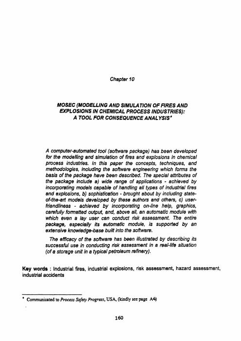
Chapter I 0

MOSEC (MODELLING AND SIMULATION OF FIRES AND EXPLOSIONS IN CHEMICAL PROCESS INDUSTRIES):

A TOOL FOR CONSEQUENCE ANALYSIS'

A computer-automated tool (software package) has been developed for the modelling and simulation of fires and explosions in chemical process industries. In this paper the concepts, techniques, and methodologies, including the soffware engineering which forms the basis of the package have been described. The special attributes of the package include a) wide range of applications - achieved by incorporating models capable of handling all types of industrial fires and explosions, b) sophistication - brought about by including state- of-the-art models developed by these authors and others, c) user- friendliness - achieved by incorporating on-line help, graphics, carefully formatted output, and, above all, an automatic module with which even a lay user can conduct risk assessment The entire package, especially its automatic module, is supported by an extensive knowledge-base buitt into the software.

The efficacy of the software has been illustrated by describing its successful use in conducting risk assessment in a real-life situation (of a storage unit in a typical petroleum refineryj.

Key words : Industrial fires, industrial explosions, risk assessment, hazard assessment, industrial accidents

- - - - - - --

Communicated to Process Safety Progress, USA, Wndly see page A4)

INTRODUCTION

Likelihood of fires and explosions are two of the major hazards associated with chemical process industries.

Explosions may be caused by several factors:

a) Pressure in a vessel or a pipe rising above critical limits due to excessive inflow of chemicals caused by a malfunctioning of flow controls - as happened at Flixborough(Less, 1996; Khan and Abbasi, 1997a; Marshall, 1987).

b) Leakage of flammabie material, which may then mix with air, and form a vapour cloud. The cloud may drift until meeting a source of ignition and exploding.

c) Pressure in an equipment rising above critical limits due to runaway reaction (generation of gases andlor heat).

d) Ignition of a flammabie chemical in confinement causing building of pressure (due to heat load and combustion products) far above safety pressure.

e) Boiling of chemical in the confinement due to absorption of external heat, thereby generating overpressure.

f) Failures of chemical storage vessels due to fracture, development of cracks, or corrosion.

g) Release of highly pressurised fluid through a narrow opening (crack, leak from joints, leakage of gasket, etc.) causing sudden phase change which may develop overpressure and generate shock waves.

Fires occur more frequently in chemical process industries than other types of accidents eventhough a large number of them are put off before significant damage is done. But major fires can be very destructive. Fires are &Q among the most frequent causes of explosions.

Fires can break out for various reasons:

i) ignition of flammabie chemical exiting from an opening (valve or crack);

ii) continuouslinstantaneous release of flammable gas which on meeting a source of ignition catches fire;

iii) continuouslinstantaneous release of liquid flammable chemical either through regular openings such as valves or through irregular opening such as leaks or cracks, creating pools of liquid which on ignition catch fire.

The destructive impact of explosion generally covers wider area than the region-of- impact of a fire. Secondly, except in certain cases when ambient conditions conspire to enable very rapid spread of a fire, most fires take time to consolidate. If emergency preparedness measures are in place, this time proves crucial in enabling to control the fire. On the other hand, when an explosion takes place it does so instantly, giving no time to escape from it.

In very large situations, explosions in chemical process industries are either caused by fire, or lead to a fire. It is therefore necessary to study explosions and fires together eventhough they are essentially two very different types of events.

MECHANISMS OF THE DAMAGE CAUSED BY EXPLOSIONS AND FIRES

An explosion in air is a sudden release of energy accompanied by the production of a shock wave and loud noise. It has the potential to injure living systems and damage assets such as buildings and the environment. The violence of an explosion depends on the rate at which energy is released.

Explosions in chemical process industries are associated with sudden release of physical energy, chemical energy, or both.

Physical energy IS manifested as pressure energy in gases, strain energy in metals or electrical energy. Examples of the violent release of physical energy are the explosion of a vessel due to high gas pressure and the sudden rupture of a vessel due to brittle fracture (Lees, 1991). In such explosions, the violence of which depends upon the internal pressure, damage may be caused by a blast wave from the expanding gas or by portions of the disrupting container. At times parts of such a vessel may be shot away to hundreds of meters. Explosions often occur if pressure on a liquefied gas (which seldom exceeds 40 bars as this is the critical pressure of most common liquefied gases) is suddenly released (Marshall, 1987).

Chemical explosions involve energy derived from a chemical reaction. Explosion of a vessel due to combustion of flammable gas, and explosion of a reactor caused by decomposition of reaction products in a runaway chemical reaction, are examples of accidents involving chemical energy.

As stated, an explosion may involve both kinds of energy and thus it is important to study the role of both types of energies singly and in combination in order to understand (and the control) the mechanism of industrial explosions.

Deflagration and detonation

Combustion of flammable gas may lead to two kinds of explosions: deflagration or detonation. In a deflagration the flammable mixture burns relatively slowly. For hydrocarbon-air mixtures the deflagration velocity is typically of the order of 1 mls.

In a detonation the flame front travels as a shock wave followed closely by a combustion wave which releases the energy to sustain the shock wave. The detonation front may reach velocities of the order of the velocity of sound and the hot products of combustion may have supersonic velocities. For hydrocarbon-air mixtures the detonation velocity is typically of the order of 2000-3000 mls.

A detonation generates greater pressures and is more destructive than a deflagration. But, a deflagration may turn into a detonation, particularly when travelling down a long pipe. Where a transition from deflagration to detonation is occurs, the deflagration velocity naturally exceeds that quoted above.

Types of explosion

Explosions in the storage or process units can be categorised in four main groups, according to their mode of occurrence and damage potential:

+ confined vapour cloud explosion-CVCE, (Baker et a/., 1983; WHO, 1984; Lunn, 1989, Catlin, 1991; Greenbook, 1992)

+ vapour cloud explosion-VCE, (Kletz, 1977; Pnrgh, 1987; Pietersen, 1990; Van den Berg, 1985; Van den Berg and Lennoy, 1993; Van den Berg, 1984);

+ boiling liquid expanding vapour explosion-BLEVE, (Birk and Cunningham, 1994; CCPS, 1989; Prugh, 1991; Venarat etal., 1993);

+ vented explosion (Catlin, 1991; Harrison and Keyre, 1987; Cates and Bimson, 1991; Kalghatgi, 1983).

These explosions are initiated either by the thermal stratification of the liquid and vapour or by such high explosion shock waves, which have sufficient strength to rupture the reactionlstorage vessels or conduits. An explosion may or may not be accompanied with fire; it depends upon the type of explosion and the chemical involved in the explosion. A brief description of each type of explosion is presented below.

Boiling Liquid Expanding Vapour Explosion (BLEVE)

BLEVE is caused by a sudden release from confinement of a liquid at a temperature above its boiling point. The sudden decrease In pressure results in explosive vaporisation of a fraction of the liquid and a cloud of vapour and mist, with accompanying blast effects. If the material is flammabie and an ignition source is present, a fire ball may be formed.

Generally, BLEVE occurs when a pressurised vessel containing a flammable liquid is exposed to fire which may weaken the vessel walls, leading to ruptures. The mechanism is as detailed below:

When a vessel containing liquid under pressure is exposed to fire, the liquid heats up and the vapour pressure rises, increasing the pressure in the vessel, eventually activating the pressure relief valve. The iiquid level in the vessel falls as the vapour is released to the atmosphere. The liquid is effective in cooling that part of the vessel wail which is in contact with it, but the vapour is not. The portion of the vessel wall which has the benefit of liquid cooling falls as the liquid vaporises. Afler a time, metal which is not cooled by liquid becomes exposed to the fire; the metal becomes hot and weak and may then rupture. This can occur eventhough the pressure relief valve is operating correctly. A pressure vessel is designed to withstand the relief valve set pressure, but only within the design temperature conditions. If the metal has its temperature raised, it may lose strength sufficiently to and get ruptured.

A BLEVE of a vessel containing a flammable liquid gives rise to the following effects: ( I ) blast wave, (2) fragments and (3) fireball.

Vapour Cloud Explosion (VCE)

The delayed spontaneous ignition of a vapour cloud of flammabie chemical in a unconfined or semi-unconfined (congested boundary) space results in vapour cloud explosion (VCE) or unconfined vapour cloud explosion (UVCE). Until the early 1980s a vapour cloud explosion (VCE) was generally referred to as an unconfined vapour cloud explosion (UVCE). However, since in combustion of a vapour cloud the overpressure tends to occur due to the presence of structures and obstacles and of partial confinements, the term 'unconfined' is now generally omitted.

A vapour cloud explosion is one of the most serious hazards in the process industries because a vapour cloud may drift some distance from the point where the leak has occurred before exploding; it may thus threaten areas lying far away from the source of the vapour cloud.

The importance of the vapour cloud explosion hazard has grown in recent years. Whereas in earlier times the major disasters tended to be those caused by explosives, including ammonium nitrate, many of the recent disasters have been due to vapour cloud explosions.

Two approaches are used to assess vapour cloud explosions: one is the TNT equivalent model and the other is multi-energy method (Van den Berg and co-workers, 1984, 1985,1991,1993). They are briefed here.

In the TNT equivalent model the explosion is taken to be equivalent to that of a TNT explosion. This model is empirical but, within its limitations, has served the study of explosions rather well.

The TNT equivalent model is based on a single parameter: the mass of TNT. It is made more flexible by taking into consideration a second parameter -the height above ground at which the explosion occurs. Higher the point of explosion lower is the overpressure near the epicentre. The use of an arbitrary assumed explosion height helps in obtaining better fits to overpressure assessed from damage in actual explosion.

The TNO vapour cloud explosion model is the multi-energy (ME) model described by Van den Berg (19&Q), Van den Berg, (1985), Van den Berg et a/., (1991), Van den Berg and Lennoy (1993). This model allows the peak overpressure, peak dynamic pressure and duration time to be estimated.

The model recognises the role of partial confinement in vapour cloud explosions. it is assumed in the model that the explosion in those parts of the cloud which are confined is of much higher strength than in those where it is unconfined. The method involves estimating the combustion energy available in the various parts of the cloud and assigning to each part an initial strength.

Confined vapour cloud explosion (CVCE)

When an explosion occurs in a conflned space (within a closed boundary) such as a vessel or a pipe - triggered by excessive pressure development either due to runaway reaction process, overfilling, or absorption of heat from external sources - it is called CVCE. Liquids of low boiling points, flammable gases, or highly reactive chemicals processed under extreme conditions, are most likely to generate CVCE. A CVCE occurs when the pressure in a confinement reaches certain critical limits beyond safety level.

The explosion energy leading to the bursting of a vessel is a function of the initial pressure, which in turn depends on the failure scenario. The higher the pressure, the stronger the explosion.

If the vessel fails due to build up of pressure inside it beyond critical levels, and because the pressure relief valve has failed, the vessel will burst at a pressure which is some multiple of the design pressure.

If the vessel fails due to material defect, wear-and-tear, or corrosion, or powerful impact, the burst pressure will be the operating pressure.

If fire engulfment occurs, but with the pressure relief operating, the pressure at the moment of vessel rupture will be the accumulation pressure. This is the typical scenario of a BLEVE. In principle, the energy available will be partitioned as energy in (1) vessel expansion, (2) vessel rupture, (3) blast, and (4) fragments.

The impact of CVCE can be observed over a much larger distance than UVCE. Due to its large area of impact and more severe shock waves CVCE also has greater potential of causing secondary, tertiary and higher order accidents (domino I cascading effects).

Vented explosion

Vented explosion is a phenomenon observed because of the formation of fire torch in a vessel due to ignition of a flammable chemical (gas or liquid) at release point. In this situation the flame front may move backwards in the vessel with high speed and ignite the contents of the vessel resulting in excessive pressure development leading to an explosion. In vented explosion flame front speed may reach over 50 m/s. It is differentiated from CVCE by its mode of initiation and its damaging effects. Eventhough vented explosion also generates shock wave, over pressure, heat load, and missiles, its damaging effects are generally confined to smaller areas than the impacts of CVCE. The intensity of the damaging effects are also lower: a vented explosion typically generates shock (blast) wave of 330 to 500 rn/s and overpressure of 0.3 to 10 atm.

Fire

Fire occurs when a source of heat comes in contact with a combustible material. If a combustible liquid or solid is heated it evolves vapour, and if the concentration of vapour is high enough it forms a flammable mixture with the oxygen of the air. if this flammable mixture is then heated further to its ignition point, combustion starts. Similarly, a combustible gas or vapour bums if it is heated to a sufficiently high temperature.

Three components must be present if fire is to occur: ( 4 ) fuel, (2) oxygen, and (3) heat. These components are often called as 'the fire triangle'. If one of the components is missing, fire does not occur and if one of them is removed, fire is extinguished.

Fire is generally initiated by an external source (such as a spark). It is then perpetuated and intensified by the combustion process itself. The three components essential for a fire also provide us the clue on how to model the fire, indeed how to fight it.

The first step towards stopping a fire is to cut off the fuel. This is particularly relevant for fires caused by leaks in process plant. The second method is to remove heat. This is usually done by putting water on the fire. The third method is to stop the supply of oxygen. This may be effected in various ways, including the use of foam or inert gas.

When fire reaches close to a vessel or it transfers to it a heat load which may be large enough to overcome the creep of the material of constwction of the vessel or overheat its contents generating excessive pressure, an explosion may result. Important aspects of

modelling fire -related accidents are: flame height, flame merging phenomena in fires in close proximit~, the effect of wind on flame tilt and length, and heat load.

Fire Is among the most common accident that occurs in chemical industries; it is estimated that fire of large or small magnitude occurs at least once a year. There is considerable possibility that one among ten fires can generate heat load large enough to precipitate a significant accident.

In a fire, the heat is not uniformly distributed. In some parts, particularly near the edge of the fire, the heat balance may be only just positive. The fire extinguishers should be directed to those parts of the fire so as to hit it at its weakest points.

Fire normally grows and spreads by direct burning, which results from impingement of the flame on combustible materials, by heat transfer or by movement of the burning material.

All the three modes of heat transfer -conduction, convection, and radiation are signfticant in heat transfer from fires. Conduction is important particularly in allowing heat to pass through a solid barrier and ignite material on the other side. Most of the heat transfer from fires, however, is by convection and radiation. It is estimated that in most fires some 75% of the heat emanates by convection. The hot products of combustion rising from a fire typically have a temperature in the range 800-1200°C and density a quarter that of air. Radiation is the other main mode of heat transfer. Although it usually accounts for a small proportion of the heat issuing from the fire, radiated heat is transferred directly to nearby objects, does not go preferentially upwards and crosses open spaces. For these reasons it is generally the most significant mode of transfer as far as the study of accidents is concerned.

Types of tire

Industrial fires are of four types: flash fire, fire ball, pool fire, and jet fire. A brief description of each is presented below.

Flash fire

A flash fire occurs when a vapour cloud, formed from a leak, is ignited without the creation of significant overpressure. Such flash fires are not uncommon in chemical process industries. If the ignition is prompt the cloud may be modest in size, but if the cloud has time to spread over an appreciable part of the site and is then ignited, a major vapour cloud fire may result.

Flash fire is modelled by considering dispersion of the vapour cloud and its ignition. One of the first such models was by Eisenberg eta/. (1975) in which the vapour cloud was assumed to be a half ellipsoid. In another model of Raj and Emmons (1975), the speed of the flame propagating through the vapour cloud is taken into account. It is assumed that during the combustion of a vapour cloud there is a turbulent flame front propagating into the unburned cloud at constant velocity which is roughly proportional to the wind speed, and that at high gas concentrations there is a tall flame plume at the edge of the unburned cloud. A modified version of this model has been recommended for use by CCPS (1994) (centre for chemical process safety) in their guidelines (1994). Considine and Grint (1985) have developed graphs linking distance from flash fire to fatal injury.

Fire balls

A spontane0~~ ignition of vapour cloud not having sufficient energy to explode leads to

fire ball. This phenomenon is generally observed for high boiling yet highly flammable liquids stored or processed at extreme conditions of temperature and pressure. Most treatments of fireballs relate to liquefied gas. A distinction must be made between a fireball resulting from the bursting of a pressure vessel and the one resulting from the formation of a vapour cloud. In the former the bursting may be caused by a fire and can be part of a BLEVE or it may occur in the absence of fire. In such cases momentum forces predominate. But in the latter case buoyancy forces play dominant role. The destructive ability of fire ball is very high as the heat load generated by it is of the order of 1000 k~lm'. The fire ball radii generally vary from 100 meter to 300 meter and its impact duration from few seconds to few minutes.

The modelling of fireballs involves consideration of : (1) the fireball regime, (2) the mass of fuel in the fireball, (3) the fireball development and time scales, (4) the fireball diameter and duration, (5) the heat radiated and (6) the view factor. A fireball may be of a relatively short duration, but it passes in its life cycle through several distinct stages which need to be carefully defined if confusion is to be avoided( Roberts, 1982).

Pool fire

When a flammable liquid spills onto the ground and is ignited, a pool fire results. A fire in a liquid storage tank is also a form of pool fire, as is a trench fire. A pool fire may also occur on the surface of flammable liquid spilled onto water.

A pool fire bums with a flame which is often taken to be a cylinder with a height twice the pool diameter. In still air the flame is vertical, but in wind it tilts. Wind also causes the base of the flame to extend beyond the downwind edge of the pool, thus exhibiting flame drag. In some pool fires blowout can occur at a wind speed of about 5 mls.

The characteristics of a pool fire depend on the pool diameter. The liquid buming rate increases with diameter until for large diameters it reaches a fixed value. The heat radiated from the flame behaves similarly.

In modelling pool fires the following aspects have to be taken into account (1) flame geometry, (2) liquid buming rate, (3) flame characteristics, (4) heat radiated and (5) view factor.

Jet fire

Burning of a flammable gas issuing from a pipe or other orifice at the point of exit leads to jet fire. Jet flames have been involved in a number of accidents. Perhaps the most dramatic were the large jet flames from the gas riser at Piper Alpha(Less, 1996; Lees, IQQl ) ,

Jet flame can occur in chemical process industries, either by design or by accident. They occur intentionally in burners and flares. Ejection of flammable fluid from a vessel, pipe or pipe flange can give rise to a jet flame if the material ignites. An intermediate situation, and one which particularly concerns the designer, is where the jet flame results from ignition of flammable material vented from a pressure relief valve.

Scenarios involving jet flames are not easy to handle, since a large jet flame may have a substantial 'reach', sometimes up to 50 m or more.

Compared to pool fire and fire balls, jet flames can occur in more diverse ways. The scenario most often considered is that of a vertical flame or an upward pointing jet, in calm conditions or in wind. But a jet may point upwards not vertically but at an angle, in such a case there may be a variety of wind directions, confluent with, opposed to or across the jet. There can also be a horizontal jet too, on which the wind may act in tandem, opposed to, or across It.

IMPACT OF EXPLOSIONS AND FIRES

Overpressure/Blast waves/Shock waves

A sudden and violent release of energy causes the surrounding air pressure to rise rapidly creating a region of positive pressure known as overpressure. As the consequent 'blast' wave moves away from its source at high velocity the overpressure increases sharply to a peak value, known as the peak overpressure, and then gradually recedes. The overpressure phase is followed by a region of negative pressure or underpressure. This pressure is generally insignificant compared with the overpressure phase, although such negative pressure can cause moderate damage especially at close distances from the charge. The characteristics of blast waves have been discussed briefly by Lees (1996) and detailed accounts have been given by Baker et al. (1983), and Kinney and Graham (1 985).

Damage and injury as a result of explosion is largely a consequence of two effects, diffraction and drag. Diffraction effect is related to the peak overpressure of a blast wave as it passes over and around an object or structure. The force exerted on an object or structure during blast wave envelopment is termed diffracfion loading. The loading consists of two components: one results from the pressure differential that exists between the front and back of an objecffstructure prior to envelopment, and the second -called static loading ("crushing" forces) - results from the pressure differential between internal and external environment. When a blast wave strikes an object or structure, reflection occurs resulting in a rapid rise in pressure termed 'reflected overpressure'. As the pressure drops the blast wave bends or "diffracts" over and around the structure loading other faces.

The effect of 'drag', called 'drag loading', is related to dynamic pressure. This is the air pressure behind a shock front and unlike overpressure has no reference to ambient pressure. Forces exerted by drag loading are the result of transient winds which accompany the passage of a blast wave.

Drag loading tends to be the main cause of damage in large explosions because in case of such explosions (peak overpressure greater than about 4.8 bar), the dynamic pressure is greater than peak overpressure. In such situations objects and structures may present little resistance to blast waves. For example, buildings whose walls, windows and doors rapidly fail during blast wave interaction cause prompt equalisation of interior and exterior environments. This in turn can reduce the duration and magnitude of diffraction loading to a negligible level.

All objects and structures simultaneously suffer both diffraction and drag loading because overpressure and dynamic pressure both exist during a blast and cannot be separated. The relative importance of each load type is largely dependent on size, shape, weight and resistance of objects and stmctures. Closed or semi-closed structures, such as buildings with small openings or large tanks, etc. are vulnerable to diffraction loading, whereas, tall thin objects and buildings with large openings are vulnerable to drag loading.

In the modelling of blast wave damage, recourse is most often taken in assessing overpressure. This is probably due to its ease of measurement and estimation compared with other damage-relation criteria. However, blast wave damage is also a function of rate of pressure rise and wave duration, and these factors are also considered in some models. An impulse is also used as measure of blast damage. Impulse is a function of both overpressure and wave duration. It is often considered a better measure of blast wave damage.

Missile

Objects or their fragments may be turned to missiles as a result of energy delivered to them by an explosion and can cause significant damage to the bodies they hit.

The missiles are characterised by velocity, range and penetration. The missiles may be either primary or secondary. Primary missiles consist of casing andlor container fragments from the exploded unit, whereas secondary missiles consist of fragments from objects located close to the explosion source which have interacted with the blast wave.

The missiles generated from cased charges have initial energy of the order of 20% - 60% of the explosion energy. The initial velocity of the missile can be calculated from.

E = 1 1 2 ' ~ ' ~ ~

Where, E denotes energy associated with fragments (J), M is mass of fragment (kg), and V is velocity of missile (mls).

The range of a missile is calculated using an empirical equation (CCPS, 1989; CCPS, 1994; Davies, 1993).

X = ( ~ " l k ~ d ) (In UN)

Where X denotes the range (m), W fragment mass (kg), U initial fragment velocity (mls), V fragment velocity (rnls), k is a constant (0.002 velocity supersonic. 0.0014 velocity subsonic) and Cd is the drag coefficient.

Depending on the momentum they carry when they hit an object, the missiles may cause damage varying from the superficial to the devastating. According to Explosives Storage and Transport Committee (ESTC), UK, missile with -80 J of kinetic energy may prove lethal to humans Davies (1993). The ESTC suggests that one fragment per 56 square meten provides individuals who are out in the open with a 1% chance of being hit. Buildings and other relatively large objects can be crushed or penetrated by missiles leading to minor hazards, such as, falling debris and glass breakage. However, impulsive loading during impact, especially from large heavy missiles, presents the greatest indirect hazard. This is because impulsive loads may instigate or encourage collapse of structures andlor escalate the amount and rate of falling debris and glass breakage. The missile may also lead to the initiation of domino effects (Khan and Abbasi, 1997b; 1997c), so

much so that the secondary or higher order accidents thus caused may generate more damage than the primary event.

The department of industrial safety, The Netherlands has proposed equations relating the probability of fatality to skin penetration based on fragment velocity and mass (Pasman et el., 1992).

For fragments of less than 0.1 kg.

Pr = -29.15+2.101nS

where S equals ~9'"' For fragments between 0.1 kg and 4.5 kg,

Pr = -17.56 + 5.30 InS

For fragments greater than 4.5 kg,

Pr = -13.19 + 10.54 InV

where M is mass of fragment (kg), and V is fragment velocity (mls).

Thermal damagehnjury

The damage potential of a fire in terms of heat load generated by the fire is a function of the type of release, flammability and the quantity of the chemical involved, strength of ignition source, and finally the type of fire. For example - flash fire and fire ball have higher damage potential compared to pool fire and jet fire for the same chemical and the same quantity. However, the occurrence of particular type of fire event is dependent on the release mode, type of operation, operating conditions and modelstrength of ignition source. The anatomy of industrial fire has been discussed by Roberts,l982; CCPS, 1989; Pietersen, 1990; Prugh, 1994; Lees, 1996. Experimental studies (Eissenberg et al., 1975; CCPS, 1994) have suclaested that a heat load of 37 kwlm2 is sufficient to cause -- damage to other installations operating under normal (atmospheric) operating conditions. If a unit is operating under extreme conditions of temperature and pressure the fire makes the unit even more;ulnerable to failure.

Vis a vis impacts on humans, correlations for both fatal and non-fatal burn injuries have been derived by Eisenberg et 81. (1975). Such impacts depend very much on the source of radiation. One such source which is of long-standing interest is a flare. Another source of thermal radiation which has received increasing attention is a fireball. A fireball is better defined than most other types of fire to which people may be exposed; it is also one of the fire hazards most likely to give rise to a large number of serious injuries.

Besides scorching, fire may also induce lethality by causing rapid depletion of oxygen in the atmosphere due to the consumption of oxygen in the combustion process. This impact is generally limited to the immediate vicinity of the fire. Of importance also are the health effects arising from exposure to the fumes generated as a result of fire. These fumes may include toxic gases, such as sulphur dioxide from the combustion of carbon disulphide and nitrous oxides from a fire involving ammonium nitrate.

When the thermal radiation load on a process vessel becomes intense (greater than 37 kw1m2), the pressure and temperature inside the vessel increase rapidly. Normally, the pressure relief valve opens when the corresponding set pressure is reached. It may open and close several times and may eventually remain open if the thermal inflow to the tank is sufficient to maintain the necessary level of vaporisation. If the thermal radiation inflow continues unchecked, the shell temperature and vapour space pressure increase to levels that weaken the materials of construction and a rupture ensues with a large energy release. Under such circumstances, high velocity fragments of the vessel can be propelled over long distances.

MOSEC (MODELLING AND SIMULATION OF FIRES AND EXPLOSIONS IN CHEMICAL PROCESS INDUSTRIES)

Among the available software packages specialising in assessment of risk due to explosion and fires are BLAST (Van den Berg, 1980), FIRE2 (Pritchard and Binding, 1992), REAGAS (Van den Berg, 1989), SAFETI (Pitbaldo and Naipanis, 1989), SAVE (TNO, 1992), EFFECTS (TNO, 1991), RlSKlT (VTT, 1993), CMBWAT (Madsen and Wagner, 1994). MOSEC has aimed to substantially improve upon these in terms of:

* greater applicability - achieved by incorporating large number of models and modules for studying a wider range of situations;

greater sophistication - achieved by incorporating the most refined and recent models and methodologies; also by using one of the most advanced coding tool viz C++;

greater user-friendliness - achieved by adding features such as 'automatic module' so that even a person not well-versed in chemical engineering or risk assessment can gainfully use the tool. The architecture, internal contents, and capabilities of MOSEC are described below.

Structure

MOSEC (Figure 1) has four main modules namely, i) accident scenario generation, ii) damage effect calculation, iii) graphics interface and iv) user interface. The hierarchy of these modules is shown in Figure 2. Each module has its own sub-modules, function, and attributes.

Accident scenario generation module

This module helps the user to generate credible scenario of all likely ways in which fire and/or explosion may occur in an industry. This step is of overwhelming importance because the more realistic an accident scenario, the more accurate is forecasting of the type of accident, its consequences, and associated risks. Consequently this step holds the key to development of the most appropriate and effective strategies for crisis prevention and management.

Each accident scenario is basically a combination of different likely accidental events that may occur in an industry. Such scenarios are generated based on the properties of chemicals handled by the industry, physical conditions under which reactions occur or reactantslproducts are stored, geometries and material strengths of vessel and conduits, valves and safety arrangements etc. External factors such as site

Lccidtnt ---+ roenu'io generation

I +--.....--...*. J

h s e . c ) U N C ~ I ~ I $ ~ I C e s t l u t r o n

, Indurt~ial fin . In t m r l

e 8 s i ; n

Pigum 2. Objects associated uith HOSE ad the nessage f lw a c m t h

characteristics (topography, Presence of trees, ponds, rivers in the vicinity, proximity to other industries or neighbourhoods etc.) and meteorological conditions are also considered. In the available software packages such as BLAST (Van den Berg, 1980), FIRE^ (Pritchard and Binding, 1992) this concept of risk assessment has been used to some extent But the level of sophistication needs to be enhanced substantially by using advanced models of thermodynamics, heat transfer, and fluid dynamics to generate more realistic accident scenarios. Furthermore, the user-friendliness of these packages have some limitations.

For example Olaniya et 81. (1996) have presented a risk assessment case study of a fertilizer plant. A number of accident scenarios have been visualised in various units of the plant using software SAFETI (Pitblado and Nalpanis, 1989) and EFFECTS (TNO. 1991). Almost all accidents have been visualised as one-likely-mode leading to one-likely consequence. For example rupture of secondary reformer has been visualised only as a vapour cloud explosion (VCE), instantaneous hydrogen release also only as VCE; failure of associated gas pipe line also as VCE, and leak in methanator as flare (flash fire). However, storing or processing large quantities of chemicals under extreme conditions of temperature and pressure may generate diverse possibilities of accidents in each situation. For example rupture of secondary reformer would indeed cause explosion as visualised by Olaniya et al. (1996) but there would also be sufficient unburned chemical which may lead to fire. Hence one of the credible scenarios would be VCE followed by fire. Unless the software tool is versatile enough to lead the user to all likely situations, such credible accident scenarios may be omitted thereby seriously effecting all subsequent steps in risk analysis and management.

In MOSEC all credible accident scenarios are carefully generated based on the properties of chemicals, operating conditions, and details of the processlstorage units. Once accident scenarios have been developed, they are processed for further verification and consequence assessment. For the same unit and same operating conditions several plausible accident scenarios are visualised. All-in-all this option helps in simulating the various likely accidents, and characterising the worst plausible ones.

Automatic scenario generation sub module (option):

To help a user not well-versed with risk assessment, a knowledge-based expert submodule (automatic scenario generation option) has been included to help the user in developing accident scenarios.

This is a derived object from the main accident scenario object. It deals with the knowledge-base which decides the accident scenario for a set of information provided by the user. The knowledge base is a compendium of conditions (frames) and facts stored in as if-and-else reasoning sequences (rule network).

The combination of rules has been designed keeping the following aspects in view.

a) the output of one rule provides the input to another,

b) several rules lead to a singie hypothesis,

c) the same top event (in this case an accident scenario) may occur via different routes taken by different combinations of causative factors.

The information provided by the user is passed on to the knowledge base which examines whether the information satisfies the conditions necessary for a credible accident; the latter is defined as the accident which is within the realm of possibility ( i.e, probability higher than 1'E-06 lyr) and has a propensity to cause significant damage (at least one fatalityl. This concept comprises of both probable damage caused by an accident and probability of its occurrence (Less, 1996; Ale, 1991: Hagon, 1984, HSE, 1988). There may be a type of accident which may occur very frequently but would cause little damage. And there may be another type of accident which may cause great damage blrt would have very low probability of occurrence. Both are not credible. But accidents which have appreciable probability of occurrence as well as significant damage potential (as quantified above) come under the category of credible accidents. The rule network to arrive at this conclusion is shown in Figure 3.

The knowledge base has been developed in object-oriented architecture without using any expert shell, and by using heuristic and if-and-else reasoning. Forward chaining has been used to retrieve the information from the knowledge base while backward chaining is used to justify or check the retrieved information. The set of conditions on the basis of which the package decides whether an accident would occur or not for a given set of input parameters have been based on the reports of past accidents(Less, 1996; Khan and Abbasi, 1997a; Marshall, 1987) and data generated by controlled experiments simulating accidents.

Inference mechanism

The goal of the knowledge-based system is to formulate accident scenarios for a set of chemicals, equipment, operating conditions, ambient conditions, etc. The flow of control in the scenario inference engine of this knowledge based system is outlined in Figure 4.

As discussed in earlier sections, the knowledge base has been developed in the form of a frame, and a rule network (if-and-else reasoning). An internal inference mechanism is used to propagate the faults through these frames to the network till the final set of results are arrived at. The frame system is organised into a hierarchy which supports inheritance of the common attributes. The mapping starts from the initial object identification to estimation of explosion (elements of explosion object domain) and fire (elements of fire object domain). The algorithm incorporated here for rule justification (attributes with conditions) is based on the criteria of minimum condition satisfaction. This is applied throughout the system, from beginning of mapping to final state (forward chaining). Once this mapping is complete, the results are checked by backward chaining to identify any discrepancy and to verify the logical sequence. The combination of these two mapping techniques (forward and backward) make the inference engine more reliable, in terms of quality of results.

Userdefined scenario generation sub module (option):

In this option the user defines the accident scenario on the basis of hislher knowledge and experience. For example, failure of a liquefied petroleum gas storage vessel can be visualised through various accident scenarios such as: leakage followed by UVCE, fire accompanied by CVCE, jet fire, etc.

The user considers these possibilities and chooses one Or more of the likely modes of accidents. These decisions become inputs to the subsequent analysis by IvlOSEC. For

Rule 1

NF-3

Accldenl roenerlo

BLEVE ball

followed by fire

Figure 3. Rule network for the accident scenario BLEVE followed by fire ball

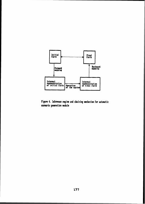
~ n i t i a ~ - . . . . ...{-I

Figwe 4. Inferme engine and chaining rrechanisrr for autonatic s a w i o genesation d u l e

example; accidental release of propylene under pressure may be visuallsed by following accident scenarios;

i) CVCE followed by flash fire or fire ball.

ii) VCE followed by pool fire or flash fire.

iii) BLEVE followed by fire ball.

iv) Fire ball.

Of these accident scenarios, the first one has the maximum damage potential. The probability of consequent damage can be made low by: a) providing high pressure safety valve, b) making provision for the availability of sufficient quantity of inert gas in times of emergency to dilute the concentration of propylene in atmosphere, and c) providing means for rapid cooling of the vessel when such need arises. The other three scenarios can likewise be developed and studied for evolving appropriate damage prevention/control strategies.

Damage effect calculation module

This module consists of state-of-the-art mathematical models for simulating the accidents chosen as credible in the previous step. This module works out the scale and the characteristics (type of accident, damage potential, percentage of lethality, and damage radii) of the accidents, the types of damaging impacts (shock waves, heat loads, missiles, etc.) they may cause, and their area of impact. The output of this module quantifies impacts such as peak overpressure, shock wave velocity, shock wave duration, heat load, missile velocity, damage radii of different impacts, and probabilities of causing lethality. The output of the consequence analysis has been so formatted that it can be directly used in report without editing. Moreover, using these results it is very easy to draw damagelrisk contours. The main module consists of two sub modules, one each devoted to explosion and fire (Figure 5). The mathematical models used in these submodules are listed in Tables I and 2.

Graphic interface module

This module enables visualisation of risk contours in context of the site of accidents. The option has two facilities: (i) site drawing, and (ii) contour drawing.

The site drawing option enables the user to draw any industrial site layout using freehand drawing or using any already defined drawing tool. The contour drawing option has the facility for drawing various damagelrisk contours over the accident site. The contours can be drawn in different shapes and sizes as per the requirement of the user.

User interface module

This module deals with the handling of data file, scenario file, output file and flow of information. This module also works as 'information manager': it provides the necessary information to each modulelsubmodule for carrying out desired operations, and stores the results in different files. Besides this, it also provides all commonly used file operations such as copying, deleting, consoling and printing.

This option also provides facility for modification or upgradation of knowledge base according to the need and experience of the user.

~ v c n r Models n r m c / t y p e I m p o r t a n t references

CVCE Isothermal and Adiabatic Lunn, 1989; Kayes, 1986: Davenport. 1986;

enpansion,combustion in Phylaktou & Andrew3,1991; Piater.en.1990;

confinement, and heat Scheuermann.1994; CCPS; Singh, 1960;

transfer models

uvcr Releases and diaperaion Baker at a1,1983; scilly and ~igh,ig86; ~1ugh.1981;

models, TNT equivalent Van den Berg and co-worker*. 1981,1985,1989,1993;

and multl energy modela Van Wlngerden and co-workers, 1389.1994

BLevc Thermodynamic and heat CCPS; Prugh,1991;

transfer models, empi- Johnson and Pr~tchard,l991; S~ngh,1988;

ricbl modela Venart et a1,1991; Blrk and Cuaningharn.1994;

vented Release wlth momentum. Harrison and Cyrc, 1987; Cetes and Samules.1991;

explos~on c o m v r t i o n model, flame Cater and Bzmson, 1992; Greenbook, 1992;

propagation, adiabatic

expansion, and heat

transfer models

115s11e Momentum and energy Munday.19BD; Holden and Reevea.1985;

effect balance models, emp- Hart and croft,1988; Scilly and Crowther.1992;

lrlcal models paarnan et a1,1992; Khan and Abbasl, 1997

Blast overpressure tmpuls. Dangreaux.1986; Davenport.1986;

wave models, peak dynamic Esparza, 1986; Pruph, 1991; Davies, 1993;

effect pressure mode1,charpe Greanbook.1992

distance model, and

thermodynamic model

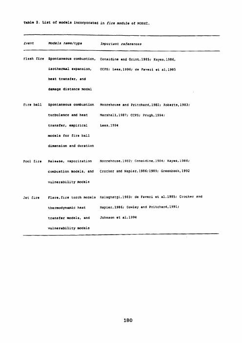
~ r b l a 2 . List of models InCOrpOrated in fire module of MOSEC.

vent Models name/type Impor tan t references

Flash fire Spontaneous combustion, Considine and Grint. 1985; Kayas, 1986,

i s o t h e r m 1 expansion, CCPS; Lees, 1996; de rsveri ct a1,1985

heat tr&nsfar, and

damage distance model

n r e ball Spontaneour combustion Moorehouse and Pritchard,l982; Robcrts,l903;

turbulence and heat Marshall,l9B7; CCPS; Prugh,1991;

transfer, empirical Lees, 1991

models tor fire ball

dimension and duration

Pool frre Release, vaporirat~on Moorchouse.l9BZ; Considine.19BI; Kayss,1986;

combustion models, and Crocker and Napler,1986;1989; Graenbook,l992

vulnerability models

Jet frre Flare,flre torch models Kblaghatg1.1983; de Faveri et a1.19851 Crocker and

t h e r m o d y n d c heat Napler,1986; cowley and Pritchard.1991:

transfer models, and Johnson at a1,1994

vulnerability models

. W l o s i o n

, Peak o v e r

. Shck wave

. Rrrrtion of shock wave ,

. l l iss i lr e f f ec t

. Heat

Danage effect calculation

Explosion Firr

L ......-.- 1

Pool f irr

Vented

lHSIANCE

. Heat load , . ., n , Duration of

Figwe 5 . the internal architecture of danage effect calculation podule

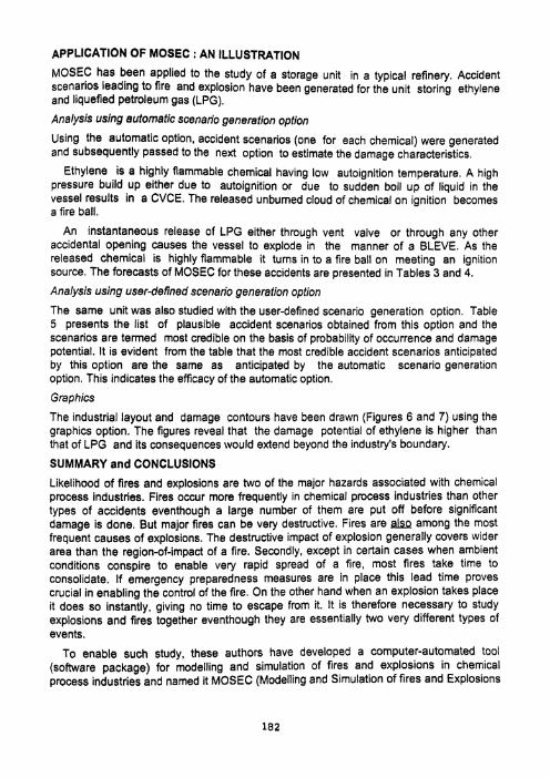
APPLICATION OF MOSEC : AN ILLUSTRATION

MoSEC has been applied to the study of a storage unit in a typical refinery. Accident scenarios leading to fire and explosion have been generated for the unit storing ethylene and liquefied petroleum gas (LPG).

Analysis using automatic scenario generation option

Using the automatic option, accident scenarios (one for each chemical) were generated and subsequently passed to the next option to estimate the damage characteristics.

Ethylene is a highly flammable chemical having low autoignition temperature. A high pressure build up either due to autoignition or due to sudden boil up of liquid in the vessel results in a CVCE. The released unburned cloud of chemical on ignition becomes a fire ball.

An instantaneous release of LPG either through vent valve or through any other accidental opening causes the vessel to explode in the manner of a BLEVE. As the released chemical is highly flammable it turns in to a fire ball on meeting an ignition source. The forecasts of MOSEC for these accidents are presented in Tables 3 and 4.

Analysis using user-defined scenario generation option

The same unit was also studied with the user-defined scenario generation option. Table 5 presents the list of plausible accident scenarios obtained from this option and the scenarios are termed most credible on the basis of probability of occurrence and damage potential. It is evident from the table that the most credible accident scenarios anticipated by this option are the same as anticipated by the automatic scenario generation option. This indicates the efficacy of the automatic option.

Graphics

The industrial layout and damage contours have been drawn (Figures 6 and 7) using the graphics option. The figures reveal that the damage potential of ethylene is higher than that of LPG and its consequences would extend beyond the industry's boundary.

SUMMARY and CONCLUSIONS

Likelihood of fires and explosions are two of the major hazards associated with chemical process industries. Fires occur more frequently in chemical process industries than other types of accidents eventhough a large number of them are put off before significant damage is done. But major fires can be very destructive. Fires are among the most frequent causes of explosions. The destructive impact of explosion generally covers wider area than the region-of-impact of a fire. Secondly, except in certain cases when ambient conditions conspire to enable very rapid spread of a fire, most fires take time to consolidate. If emergency preparedness measures are in place this lead time proves crucial in enabling the control of the fire. On the other hand when an explosion takes place it does so instantly, giving no time to escape from it. It is therefore necessary to study explosions and fires together eventhough they are essentially two very different types of events.

To enable such study, these authors have developed a computer-automated tool (software package) for modelling and simulation of fires and explosions in chemical process industries and named it MOSEC (Modelling and Simulation of fires and Explosions

Fertilizer industry

Popuious village

Figure 6. Damage contours indicating the impact area of an accident in LPG storage vessel; 75% probability of damage (A), 50% probability of damage (B), and 10% probability of damage (C)

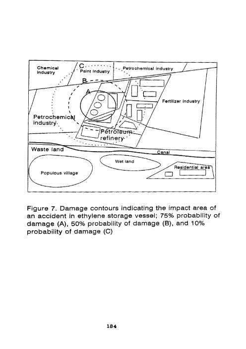
Fertilizer industry

Populous village

Figure 7. Damage contours indicating the impact area of an accident in ethylene storage vessel; 75% probability of damage (A), 50% probability of damage (B), and 10% probability of damage (C)

ÿ able 3. The Output of MOSEC for accident scenario CVCE followed by fire ball

MOSEC IcI Khan i abbbsi, Pondicherry-605 014, 1ndla

parameters Values

CONFINED VAPOR CLOUD EXPLOSION

Explosion characteristics

Total energy released (kJ) = 5.6Et07 Adiabatic energy lost due to expansion of gas(kJ) = 2.OE+06 Energy associated wlth shock wave (kJ) = 2.5E+07 Energy lost in fracture/plastic

deformation of material (kJ) = 7.6Et04 Energy available for bursting (kJ) = 4.3E+07 Energy released as heat (kJ) = 2.8E+07 Radiation heat flux (kJ/sq.m) = 5.OE+01

Shock wave characteristics

Peak over pressure D,~ration of shock wave (ms) Variation of over pressure with time ikPa/s) Shock wave velocity in air (m/s) Particle velocity behind the shock wave (m/s) Dynamic pressure (dimensionless) Reflected overpressure ikPa) Over pressure impulse (positive phase) (kPa/s)

Missile characteristics

Mass of the fragment (kg) = 5.0 Initial velocity of fragment (m/s) = 2.1E+02 Kinetic energy associated with fragment (kJ) = l.lE+05 Fragment velocity at 250 m from epicentre (rn/s) = 1.27Et02

Penetration ability (estimated uslng empirical models)

Penetration ability on concrete structure (m) = 6.2E-02 Penetration ability on brick structure (m) = 4.9E-02 Penetration ability on steel structure (m) = 1.3E-02

FIRE BALL

Radius of fire ball (m) = 384.2 Duration of fire ball (5) = 157.0 Energy released by fire ball (kJ) = 6.7E+ll Area of fire ball (sq.m) = 1.8E+06 Radiation heat intensity (kJ/sq.m) = 4.1€+05

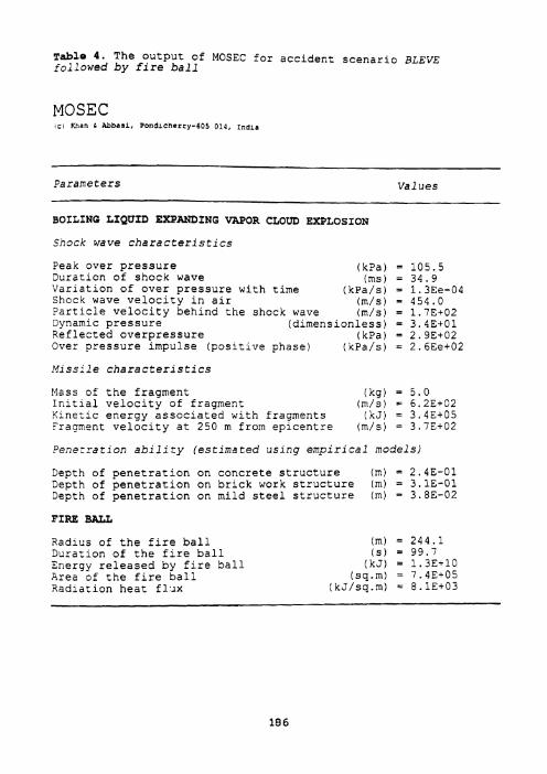
Table 4 . The o u t p u t of MOSEC f o r a c c i d e n t s c e n a r i o BLEVE fol iowed by f i re b a l l

MOSEC I C I Khan 6 Rbbaai. Pondl~herry-605 014, I n d ~ a

Parameters Va 1 ues

BOILING LIQUID EXPANDING VAPOR CLOUD EXPLOSION

Shock wave c h a r a c t e r i s t i c s

"ask ove r p r e s s u r e (kPa) Durat ion of shock wave (ms) V a r i a t i o n of o v e r p r e s s u r e wi th t ime ( k P a / s ) Shock wave v e l o c i t y i n a i r (m/s ) ? a r t l c i e v e l o c i t y beh ind t h e shock wave (m/s ) Dynanic p r e s s u r e ( d i m e n s i o n l e s s ) Ref l ec t ed o v e r p r e s s u r e (kPa) Over p r e s s u r e impu l se ( p o s i t i v e phase ) ( k P a / s )

K i s s l l e c h a r a c t e r i s t i c s

?lass of t h e f ragment (kg ) = 5 . 0 I c i t l a l v e l o c i t y of fragment (m/s) = 6.2Et02 K i n e t i c e n e r g y a s s o c i a t e d wi th f ragments (kJ) = 3 .4Ei05 'ragrrent v e l o c i t y a t 250 m from e p i c e n t r e (m/s ) = 3 . 7 E + 0 2

F s n e z r a t i o n a b i l i t y ( e s t i m a t e d u s l n g e m p i r i c a l models)

Deptn of p e n e t r a t i o n on c o n c r e t e s t r u c t u r e ( m ) = 2.4E-01 3epth of p e n e t r a t i o n on b r i c k work s t r u c t u r e (m) = 3.1E-01 3eptn of p e n e t r a t i o n on mild s t e e l s t r u c t u r e ( m ) = 3.8E-02

FIRE BALL

4adius of t h e f i r e b a l l ( m i = 244 .1 Duracion of t h e f i r e b a l l ( 5 ) = 9 9 . 7 Energy r e l e a s e d by f i r e b a l l ( k J ) = 1.3E-10 Area of t h e f i r e b a l l (sq .m) = 7.4E+05 R a d l a ~ i o n h e a t f l . ~ x ( k J / s q . m ) = 8 .1Et03

~ & 1 * 5 . AcCLdCnt Scenarlol generated by urer-defined accldent scenarzo gsnerazron optLon

c.:dmlcal Accident dcendrlos Probability Damdqe MOSC credible scenailc

a s per the urcr- of occurrence potencia1 (based on damdqe defined accident lrelatlve l i n cerms of pocentlal and scenarlo optlon percent*) damage radiiX) probabllrcy)

Ez'ylene BLEVE 11 5 5

BLEVE followed by fire ball 17 125

BlEVE followed by flash flre 04 110

VVCE followed by flash Err. 07 65

CVCE followed by fire ball 1 4 1 8 5

CVCE

Flre ball

BLEVE followed by fire ball 3 4 105

CVCE followed by flre ball 08 150

BLEVt followed

by flrc ball

CVCE followed

by llre ball

CVCE 04 8 5

UVCE followed by pa01 f r r e 11 45

W C E 15 2 5

Fire ball 2 8 4 5

frequency occurrence of particular accnarlo

Pelatlve percent = sum of the probabilities of dlfferent

acczdental event

X 1adlu6 estrmatsd for 501 probabrl~ty of darnage due to various damaglng event

in Chemical process industries). MOSEC has been aimed to substantially improve upon the existing software in t e n s of: greater applicability - achieved by incorporating large number of models and modules for studying a wider range of situations; greater sophistication - achieved by incorporating the most refined and recent models and methodologies; also by using one of the most advanced coding tool viz C++; and greater user-friendliness - achieved by adding features such as on-line help, graphics, and 'automatic module' so that even a person not well-versed in chemical engineering or risk assessment can gainfully use the tool.

REFERENCES

1. Ale, B J M, (1991). Risk analysis and risk policy in the Netherlands and EEC, J Loss Prevention in Process Industries, 4(1), 58.

2. Baker, W E, Cox, P A, Westin, P S, Kulesz, J J, and Strelow, R A, (1983). Explosion hazard and evaluation, Elesvier, Amsterdam.

3. Birk, A M, and Cunningham, M H, (1994). The boiling liquid expanding vapour explosion, J. Loss Prevention in Process Industries, 7, 474.

4. Cates, A T, and Bimson, S J, (1991). Fuel and obstacle dependency in premixed transient deflagration, 13th ICODERS, Nagoya, Japan.

5. Cates, AT , and Samuels, 8, (1991). A simple assessment methodology for vented explosions. J. Loss Prevention in Process Industries, 4, 287.

6. Catlin, C A, (1991). Scale effects on the external combustion caused by venting of a confined explosion, Combustion Flame, 83, 399.

7 . CCPS, (1989). Guidelines for chemical process quantitative risk analysis, Centre for Chemical Process Safety, AIChE, New York.

8. CCPS, (1994). re and explosion guidelines, Centre for Chemical Process Safety, AIChE, New York.

9. Considine, M, (1984). Thermal radiation hazards ranges from large hydrocarbon pool fires, SRD report number R297, U K atomic energy authority.

10. Considine, M, and Crint, G C, (1985). apid assessment of the consequences of LPG releases. Gastech, 84, 187.

11. Cowley, L T, and Pritchard, M J, (1991). Large-scale natural gas and LPG jet fires and thermal impact on structures, Gastech 90, 3.6.

12. Crocker, W P, and Napier, D H, (1986). Thermal radiation hazards of liquid pool fires. In Hazards, IX, 159.

13. Crocker. W P, and Napier, D H, (1988). Mathematical models for the prediction of thermal radiation from jet fires, Preventing Major Chemical and Related Process Accidents, 331.

14. Dangreaux, J, (1986). Destructive explosion effects, Los Prevention and Safety Promotion, 5, 9.1.

Davenport, J A, (1986). Hazards and protection of pressure storage of liquefied Petroleum gases. h s s Prevention and Safety Promotion, 5, 22.1.

Davies, P A, (1993). A guide to the evaluation of condensed phase explosion, Journal of Hazardous Materials, 33, 1.

de Faveri, D M, Fumarola, G, Zonato, C, and Ferraiolo, G , (1985). Estimate flare radiation intensity. Hydrocarbon Process., 64(5), 89.

Eissenberg. N A, Lynch, C J, and Breeding, R J, (1975). lnerability Model: A Simulation System for Assessing Damage Resulting from Marine Spills, Report CG-D-736-75(Enviro control), Rockville M D., USA.

E s p a ~ a , E D, (1986). Blast measurements and equivalency for spherical charges at small scaled distances. Int. J. Impact Engineering, 4, 23.

Greenbook, (1992). Methods for determining of possible damage to people and objects resulting from release of hazardous materials, Report CPR-IGE, Voorburg, Warrington. UK.

Hagon, D 0 , (1984). Use of frequency-consequence curves to examine the conclusion of published risk analysis and to define broad criteria for major hazard installations, Chem Engng Res Dev, 62, 381.

Harrison, A J, and Keyre, J A, (1987). 'External explosions' as a result of combustion venting. Combustion Science Technology., 52, 91.

Hart, D, and Croft, T, (1988). Modelling with Projectiles, Ellis Honvood, Chichester.

Holden, P I, and Reeves, A B, (1985). Fragment hazards from failures of pressurised liquefied gas vessels, IN The Assessment and Control of Major Hazards, IChEM, Rugby 205.

HSE, (1988). The tolerability of risks formation from nuclear power stations, Health and Safety Executive , HM Stationary Office, London.

Johnson, A D, Brightwell, H M, and Carsley A J, (1994). A model for predicting the thermal radiation hazards from large-scale horizontally released natural gas jet fires. Hazards, XII, 123.

Johnson, D M, and Pritchard, M J, (1991). Large scale experimental study of boiling liquid expanding vapour explosions (BLEVEs). Gastech 90, 3.3.

Kalghatgi, G T, (1983). The visible shape and size of a turbulent hydrocarbon jet diffusion flame in a cross wind. Combust. Flame, 52, 91.

Kayes, P J, (1986). Manual of industrial hazard assessment technique, Technica Ltd., London.

Khan, F I, and Abbasi, S A, (1997a). Risk analysis of epichlohydrin manufacturing industry using new computer automated tool MAXCRED, J Loss 'Prevention in Process Industries, 10(2), 91.

Khan, F I, and Abbasi, S A, (1997~). Models of Domino effect analysis in chemical process industry, Process Safety Pr~greSS, (in press).

Khan, F I, and Abbasl, S A, (1997b). Risk analysis of a cloralkali industry situated in densely populated area, Process Safety Progress, 16(3), 172.

Kinney, G F, and Graham, K J, (1985). Explosives Shocks in Air, 2nd ed, Springer, Berlin,.

Kletz, T A, (1977). Unconfined vapour cloud explosions, AlChE Loss Prevention, 11,5.

Lees, F P, (1991 1. Piper Alpha and the plant engineer, Plant Engr, 35, 33

Lees, F P, (1994). The assessment of major hazards: a model for fatal injury from burns, Process safety and Enviroment., 728, 127.

Lees, F P, (1996). Loss prevention in CPI, Butterworths, London.

Lunn, G A, (1989). Methods for sizing dust explosion event areas: a comparison when reduced pressures are low. J. Loss Prevention in Process Industries, 2(4), 200.

Madsen, W W, and Wagner, R C, (1994). An accurate method for modelling the characteristics of explosion effects. Process Safety Progress., 13, 171.

Marshall, V C, (1987). Major chemical hazards, John Wiley & Sons, New York.

Moorehouse, J, (1982). Scaling criteria for pool fires derived from large scale experiment, In The Assessment of Major Hazards. IChEM, Rugby, 165.

Moorehouse, J, and Pritchard, M J, (1982). Thermal radiation hazards from large pool fires and fireballs - a literature review, In The Assessment of Major Hazards, IChEM, Rugby, 123.

Munday, G, (1980). Initial velocities attained by plant-generated missiles, Nuclear Engineering, 19, 165.

Olaniya, R S, Mathurkar, H N, and Deshpande, A W, (1996). Probabilistic risk assessment of fertilizer plants, 3 87-94.

Pasman, H J, Duxbury, H A, Bjordal. P, (1992). Major hazards in the process industries, : achievements and challenges in loss prevention, J Hazardous Materials, 33, 1.

Phylaktou, H and Andrews, G E, (1991). Gas explosions in long closed vessels. Combust. Sci. Technol., 77, 27.

Pietersen, C M, (199O).Consequence of accidental release of hazardous materials, J. of Loss Prevention in Process Industries. 3, 136-141.

Pitblado, R M, and Nalpanis, P, (1989). Quantitative assessment of major hazard installations: 2, Computer programs., (eds Lees, and Ang), Buttenuofihs, London.

Pritchard, M J, and Binding, T M, (1992). FIRE2 ; a new approch for predicting thermal radiation levels from hydrocarbon pool fires, Major hazards onshore and offshore, 491.

Prugh, R W, (1987). Evaluation of unconfinea vapour cloud explosions, Proceedings of International Conference of Vapour Cloud Modelling, Boston.

Prugh, R W, (1991). Quantitative evaluation of BLEVE hazards, Journal of Fire Protection Engineers, 3(1), 9-24.

P W h , R W, (1994). Quantitative evaluation of fire ball hazards, Process Safety Progress, 13(2), 83.

Raj P P K, and Emmons, H W, (1975). the burning of a large flammable vapour cloud. Combustion Inst., Joint Tech. Mtg of the Western and Central State Sections) , Pittusberg.

Roberts, A P, (1983). Thermal radiation hazard from release of LPG from pressurised storage, Fire & Safety Journal, 4, 197.

Scheuermann, K P, (1994). Studies concerning the influence of turbulence on the course of explosions. Process Safety Progress, 13, 219.

Scilly. N F, and Crowther, J H, (1992). Methodology for predicting domino effects from pressure vessel fragmentation :Hazard Identification and Risk Analysis, Human Factors and Human Reliability in Process Safety, 1.

Scilly, N F, and High, W G, (1986). The blast effects of explosions, Loss Prevention and Safety Promotion .5, 39.

Singh, J, (1988). Explosion propagation in non-spherical vessel: simplified equations and applications, J Loss Prevention in Process Industries, 1(1), 39.

TNO, (1991). EFFECTS : a software for hazard assessment, TNO Prins Mauritius Research Laboratory, The Netherlands.

TNO, (1992). SAVE : a software for hazard assessment, TNO Prins Mauritius Research Laboratory, The Netherlands.

Van den Berg, A C, (1980). "BLAST" - A 1-D Variable Flame Speed Blast simulation Code using a Flux-corrected-transport Algorithm. Report PML 1980- 162. Prins Maurits Lab., TNO, Rijswijk, The Netherlands.

Van den Berg, A C, (1984). Blast effects from vapour cloud explosion, Ninth Int. Sym, on The Prevention of Occupational Accidents and Diseases in the Chemical Industry, Lucerne.

Van den Berg, A C, (1985). The multi-energy method. A framework for vapour cloud explosion blast prediction. J. Hazardous Materials., 12(1), 1.

Van den Berg, A C, and Lennoy, A, (1993). Methods for vapour cloud explosion blast modelling, J Hazardous Materials, 34, 171.

Van den Berg, A C, Van Wingerden, C J M, and The, H G, (1991). vapor cloud explosion : experimental investigation of key parameters and blast modelling, Trans I Chern Engg, 69(B).

Van den Berg, AC, (1989). REAGAS - A Code for Numerical Simulation of 2-D Reactive Gas Dynamics. Rep. PML-1989-in-48, TNO Prins Maurits Lab. Rijswijk, The Netherlands.

67. Van Wingerden, C J M, (1989). Experimental investigation into the strength of blast waves generated by vapour cloud explosions in congested areas. Loss Prevention and Safety Promotion, 6, 26.

68. Van Wingerden, K, Peterson, G ti, and Wilkins, B A, (1994). Turbulent flame propagation in gas mixtures, Hazards, XII, 249.

69. Vernart, J E S, Rutledge, G A, Sumathipala, K and Sollows, K, (1993). To BLEVE or not to BLEVE ; Anatomy of Boiling Liquid expanding vapour Explosion, Process Safety Progress. 2, 11 2.

70. VTT, (1993). RISKIT : a software for risk assessment, The Technical Research Centre o f Finland, Tempere, The Finalnd.

71. WHO, (1984). Major Hazard Control : A practical manual, lnternafional Labour Office, Geneva.