part ii chapter iii descriptive analysis of data and...

[68]

Part II

Chapter III

Descriptive Analysis of Data and Methods and

Models

[69]

Chapter 3

Descriptive Analysis of Data and Methods and Models

3.1 Sources of Data

The study concentrates on application of different models to the data of India’s Bombay

Stock Exchange. BSE is the oldest stock exchange of India, and it accounts for a

substantial proportion of total transactions in Indian Stock Market. Period covered is

from first January, 2008 to December, 2008. Scrip’s of ten companies are analyzed in

detail. These ten companies account for 30% of total turnover of the Bombay Stock

Exchange. Daily prices are the focus of the study. All data have been taken from

www.bseindia.com, www.moneycontol.com . Further to enhance data base of the

study, data of daily equity prices of four companies from 2005-2010 are closely

analysed. The data of FII investment in 10 companies are taken from www.fiitrade.cvs.

These data relate to daily transactions conducted by FII with different companies in the

market. Thus, the Study depends on secondary data taken from website of BSE.

3.2 Methods and Models

The study unlike earlier researches does not depend on the results of any one single

model/ method of data analysis. At times, one may get type A results which are

method/model specific. Besides, each model /method has its assumptions which also

embody its limitations. Therefore, the choice of method(s)/ models revolves around

objective(s) , hypotheses and nature of data base. This has guided the choice of

methods/models in this study. The study uses regression models for data analysis.

http://www.bseindia.com/

http://www.moneycontol.com/

http://www.fiitrade.cvs/

[70]

Regression models may broadly be classified as per the following chart which does not

explicitly include RWM, Auto Vector Regression modeling etc.

Figure 5

This study concentrates on linear regression models and nonlinear regression models are

ignored. Moreover, price per unit is proportion of sales revenue and quantum of sales

Price of daily transactions is not in absolute terms but in ratio terms as the influence of

quantum of sales, which might have resulted in non-linearity, is eliminated. This study

has also focused on simultaneous regression models so as to establish link between

different prices of the day. Secondly, prices can be jointly determined in Simultaneous

Equation Model.

Regression

Linear

Regression

Non- Linear

Auto Regression

model

Simultaneous

Equation Polynomial

Exponent

Simple

Bivariate

Log Linear

Semi(Logit

and Probit)

Semi Log

Distributed Lag Model

[71]

3.2.1 Models and Methods used in the Study

1) Random Walk Model without Drift

The basic assumption of the model is that the changes in the values of the variable are

governed and guided by random rather than systematic factor. Therefore, the following

regression model of change in the particular variable is specified:

Yt -Yt-1 =∆Yt =Ut…………………………………. (1)

In the above relation, U represents influence of random factors on change in the values of

variable Y from one to another point in time.

2) Random Walk Model with Drift

Random Walk Model with Drift is a variant of model without drift:

∆Yt = β0 +Ut

Or

Yt =β0 + Yt-1+Ut……………………………………. (2)

β0, the coefficient of drift, takes cognizance of a fixed factor/value that is loaded

additionally on the influence of random factors on Yt. fixed factor influence on change,

given by Drift takes the value of Yt away from Yt-1 and Ut. Model 2 is derived from the

following auto-regression model of first order, if β1 =1 is substituted in relation 3 (See,

Harvey, 1981):

Yt =β0 + β1Yt-1+Ut………………………………….. (3)

If either model 1 or 2 fits the data well, that series emerges non-stationary. But ∆Yt, first

differences of Yt, may still be stationary. If ∆Yt also constitute non-stationary series, it

may encompass stochastic trend. In that case, first order differences with trend are taken

in regression model:

[72]

3) Random Walk Model with Drift and Stochastic Trend

∆Yt = β0+β1 Yt-1 + β2 T+ Ut ……………………………….. (4)

As non-spurious nature of time series regression modeling depends on stationary nature

of the series, Dickey-Fuller unit root test is used as a preliminary step of analysis.

Application of unit root test is outlined below by modified forms of relations 1, 2 and 4:

∆Yt = (-1)Yt-1 +Ut

=δYt-1 +Ut ……………………………………. (5)

∆ denotes first order difference operator. Model 5 is obtained if we substitute β0 =0, and

(-1)=δ, where δ=β1 in model 3/4. is the root of equation 5. If <1, then, the time series

of Yt is stationary. Other condition of stationarity is that δ is statistically significant, and

hence, it differs statistically from zero. If (-1)= δ =0 in model equation 5, =1. This

condition defines unit root problem. In this case, both Yt and ∆Yt are non-stationary. If,

however, δ<0, that is, its value is negative, then, ={1+(- δ)}<1, time series is stationary.

If δ>0, then, >1, time series approximates explosively non-stationary.

Values of non-stationary time series may be smoothed by link relatives: (Yt/Yt-1), as was

shown by Henry Moore (1914). Link relatives are proxies of first order differences of

modern day econometric analysis. Ratios of preceding and succeeding values of one or

more inter-related variables of time series are freed both from auto-correlation and non-

stationary feature. Series of link relatives may be used as substitute of first order

differences in regression models. Current literature emphasizes that, even if two or

more original series are non-stationary, their linear combination in a regression model

may still be stationary (Green, 2006). Residuals of such regression models are subjected

to Engel-Granger test. If residuals of a regression model are stationary, regression is

[73]

treated as genuine rather than pseudo. As all stationary root tests, including Dickey-

Fuller test, are small in size and low in power, this leaves probability of committal of

both type I and II errors. It is advisable to use Engel-Granger test to supplement Dickey-

Fuller test. Basic assumption of Engel-Granger test is that even if two or more individual

time series are non- stationary, their linear combination in a regression function may be

stationary. This is also the test of cointegration.

4) Unit Root Test :

ΔYt= δ Yt-1+Ut. Where Δ denotes first order difference operator (ρ-1) = δ in the model ,

if δ =0 then, ρ=1. It is this condition which is referred as unit root problem for testing

whether given time series is stationary. In such cases, δ = 0 will hold and Yt will be

non-stationary. If, however, , if δ<0, then ρ <1 the series will be stationary. If ρ >1, if

δ>0, the series will approximate the explosive Cob-Web Model (C.f Dickey Fuller,DA

and WA Fuller,1979).

5) Engel-Granger Test:

If the following regression model is used in a study, then, Engel-Granger test will be as

follows:

Yt = β0 + β1Xt +Ut …………………………………….. (6)

ΔUt = δUt-1 +et

Residuals of regression function (6) are subjected to Dickey Fuller test of unit root If the

residuals are stationary, regression function (6) is accepted as genuine rather than

spurious. In all above relations, Y represents a general class of variables, while G shows

general class of explanatory factors.

[74]

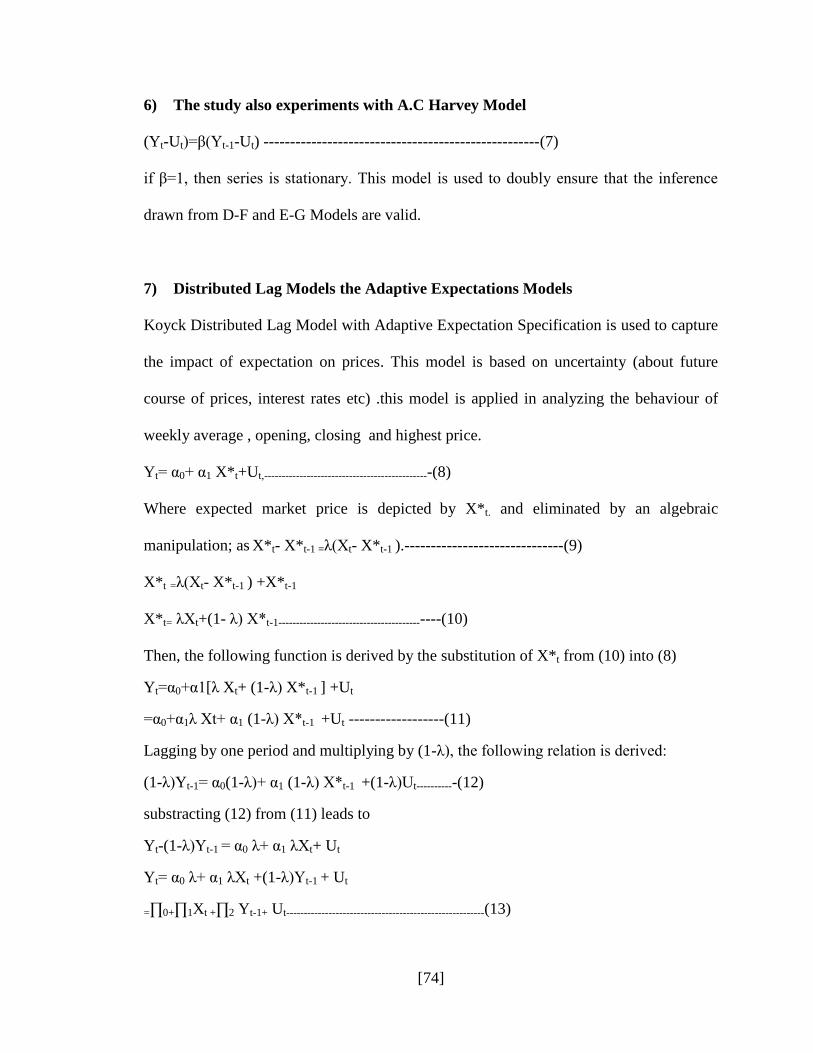
6) The study also experiments with A.C Harvey Model

(Yt-Ut)=β(Yt-1-Ut) ----------------------------------------------------(7)

if β=1, then series is stationary. This model is used to doubly ensure that the inference

drawn from D-F and E-G Models are valid.

7) Distributed Lag Models the Adaptive Expectations Models

Koyck Distributed Lag Model with Adaptive Expectation Specification is used to capture

the impact of expectation on prices. This model is based on uncertainty (about future

course of prices, interest rates etc) .this model is applied in analyzing the behaviour of

weekly average , opening, closing and highest price.

Yt= α0+ α1 X*t+Ut,-----------------------------------------------(8)

Where expected market price is depicted by X*t. and eliminated by an algebraic

manipulation; as X*t- X*t-1 =λ(Xt- X*t-1 ).------------------------------(9)

X*t =λ(Xt- X*t-1 ) +X*t-1

X*t= λXt+(1- λ) X*t-1--------------------------------------------(10)

Then, the following function is derived by the substitution of X*t from (10) into (8)

Yt=α0+α1[λ Xt+ (1-λ) X*t-1 ] +Ut

=α0+α1λ Xt+ α1 (1-λ) X*t-1 +Ut ------------------(11)

Lagging by one period and multiplying by (1-λ), the following relation is derived:

(1-λ)Yt-1= α0(1-λ)+ α1 (1-λ) X*t-1 +(1-λ)Ut-----------(12)

substracting (12) from (11) leads to

Yt-(1-λ)Yt-1 = α0 λ+ α1 λXt+ Ut

Yt= α0 λ+ α1 λXt +(1-λ)Yt-1 + Ut

=∏0+∏1Xt +∏2 Yt-1+ Ut--------------------------------------------------------(13)

[75]

Where λ is the coefficient of expectation. This regression model is subjected to Engel

Granger test of unit root of residuals to determine the stationarity of the combination of

two series under examinations. This will also highlight the co-integration of the variables

in the Model. E-G test also overcomes the high probability of both types of statistical

errors involved in hypothesis testing.

8) Distributed Lag Models the Stock Adjustment, or Partial Adjustment Model

It is note-worthy that auto-regression and distributed lag models are parts of dynamic

econometric modeling. These models play pivotal role in economic analysis. Distributed

lag models (DLM) are derivable as an extension of auto-regression model (ARM),

though DLM represents an advance version of econometric modeling in current literature.

This model is used to identify the impact of technical or institutional rigidities. This

model is used in the study to identify the impact of lagged value of dependent variable.

Koyck’s DLM with Partial Expectation Adjustment hypothesis is outlined hereunder:

Let Yt* denote the desired value of the variable under consideration at time t; which is

postulated to be the function of explanatory/pre-determined variable, Xt. This is

represented by the following regression function of these two variables:

Yt*=β0 + β1 Xt +Ut …………………………………(14)

But due to ignorance, inertia and bottlenecks is the process of adjustment of actual to

desired change in the value of the variable from preceding to current period, adjustment

actually realized is only a friction of desired adjustment. Since the desired level of Yt is

not directly observable , Nerlove postulate following hypothesis known as the partial

adjustment.

[76]

(Yt- Yt-1)= ʎ(Yt*- Yt-1)-------------------------------------(15)

Where ʎ, such that 0< ʎ≤1, is known as the coefficient of adjustment and where (Yt- Yt-

1)=actual change and (Yt*- Yt-1)= desired change.

Above function may also be written as follows:

.(Yt- Yt-1)= ʎ(Yt*- Yt-1)----------------------------(16)

Yt = ʎYt*+ (1- ʎ)Yt-1 ……………………………(17)

Substitution of value of Yt* (14) in above equation (17) gives following relation:

Yt = ʎβ0 + ʎβ1 Xt + (1- ʎ)Yt-1 + ʎUt (18)

Or

Yt = II0 +II1Xt + II2 Yt-1 +II3………………… (19)

Once we estimate short run function (19) and obtain the estimate of adjustment

coefficient ʎ (from the coefficient of Yt-1), we can easily derive the long run function by

simply dividing ʎβ0 and ʎβ1 by ʎ and omitting the lagged Y term.

9) Auto Correlation Function (ACF) and Auto Regression Model (ARM)

Auto Correlation Function (ACF) and Auto Regression Model (ARM) are used to

identify the length of lags involved in closing prices of days. Auto-correlation function, a

generalization and extension of the concept of correlation, is used if current value of

variable, Yt in time series analysis is related to its past value(s), Yt-s. Concept is

extended to random errors of estimation being related to each other. Therefore, if Yt is

linearly dependent onYt-s, coefficient of correlation of Yt with Yt-s is denoted by ρs.

For weak stationary time series, ρs is the function of s, length of the lag alone. ρs is

calculated by as follows:

ρs={Cov(Yt,Yt-s)}/[√{Var (Yt) Var(Yt-s)}]

[77]

= Cov {(Yt, Yt-s)}/{Var (Yt,)}…. (20)

=γs /γ0

Var (Yt)=Var(Yt-s) is a property of weak stationary time series.

It is inferred from relation 17 that ρ0=1 and ρs= ρ-s. Stationary time series is not auto-

correlated, only if ρs =0 for all s>0. Substitution of s=1,2,…,t-1 in relation 3 furnishes

auto-correlation coefficients of desired length of the lag. If Yt is distributed normally,

auto-correlation coefficients will also be normally distributed so that ρs^~ approximates

N(0, 1/T). T is sample size, ρs^ is the estimate of auto-correlation coefficient at lag s from

the sample. This facilitates testing of significance of auto-correlation coefficient on the

assumption of normality of distribution. Non-rejection rejection of null hypothesis, H1 at

0.05 probability level is given below:

(+-){1.96x 1/(√T)}……………………………….(21)

for s=/=0.

If ρs^ falls outside the above range for lag s, then the Null Hypothesis that the coefficient

in the population is zero is rejected. This is usual t test criterion. This test is a bit

cumbersome as it is to be applied for each length of the lag separately rather than the

testing of joint hypothesis. It is, therefore, preferable to set up the test for evaluation of

joint hypothesis for given lengths of the lag: s=1,2,3,….

ρs={Cov(Yt,Yt-s)}/[√{Var (Yt) Var(Yt-s)}]

= Cov {(Yt, Yt-s)}/{Var (Yt,)}…. =γs /γ0

[78]

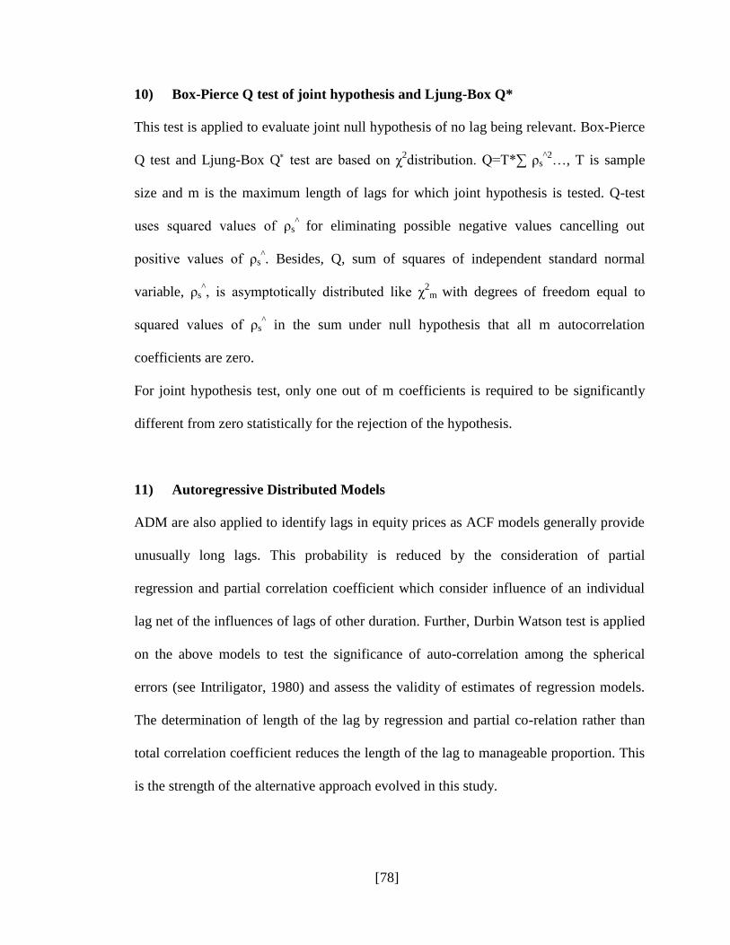
10) Box-Pierce Q test of joint hypothesis and Ljung-Box Q*

This test is applied to evaluate joint null hypothesis of no lag being relevant. Box-Pierce

Q test and Ljung-Box Q test are based on χ2distribution. Q=T*∑ ρs

^2…, T is sample

size and m is the maximum length of lags for which joint hypothesis is tested. Q-test

uses squared values of ρs^ for eliminating possible negative values cancelling out

positive values of ρs^. Besides, Q, sum of squares of independent standard normal

variable, ρs^, is asymptotically distributed like χ

2m

with degrees of freedom equal to

squared values of ρs^ in the sum under null hypothesis that all m autocorrelation

coefficients are zero.

For joint hypothesis test, only one out of m coefficients is required to be significantly

different from zero statistically for the rejection of the hypothesis.

11) Autoregressive Distributed Models

ADM are also applied to identify lags in equity prices as ACF models generally provide

unusually long lags. This probability is reduced by the consideration of partial

regression and partial correlation coefficient which consider influence of an individual

lag net of the influences of lags of other duration. Further, Durbin Watson test is applied

on the above models to test the significance of auto-correlation among the spherical

errors (see Intriligator, 1980) and assess the validity of estimates of regression models.

The determination of length of the lag by regression and partial co-relation rather than

total correlation coefficient reduces the length of the lag to manageable proportion. This

is the strength of the alternative approach evolved in this study.

[79]

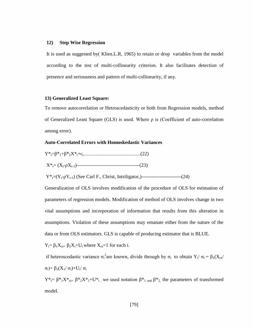
12) Step Wise Regression

It is used as suggested by( Klien.L.R, 1965) to retain or drop variables from the model

according to the test of multi-collinearity criterion. It also facilitates detection of

presence and seriousness and pattern of multi-collinearity, if any.

13) Generalized Least Square:

To remove autocorrelation or Hetroscedasticity or both from Regression models, method

of Generalized Least Square (GLS) is used. Where ρ is (Coefficient of auto-correlation

among error).

Auto-Correlated Errors with Homoskedastic Variances

Y*t=β*1+β*2X*t+ϵt.---------------------------------------------------(22)

X*t= (Xt-ρXt-1)--------------------------------------(23)

Y*t=(Yt-ρYt-1) (See Carl F., Christ, Intriligator,)------------------------(24)

Generalization of OLS involves modification of the procedure of OLS for estimation of

parameters of regression models. Modification of method of OLS involves change in two

vital assumptions and incorporation of information that results from this alteration in

assumptions. Violation of these assumptions may emanate either from the nature of the

data or from OLS estimators. GLS is capable of producing estimator that is BLUE.

Yt= β1Xoi+ β2Xi+Ui where Xoi=1 for each i.

if heteroscedastic variance σi2are known, divide through by σi to obtain Yi/ σi = β1(Xoi/

σi)+ β2(X1/ σi)+Ui/ σi

Y*t= β*1X*oi+ β*2X*1+U*i . we used notation β*1 and β*2, the parameters of transformed

model.

[80]

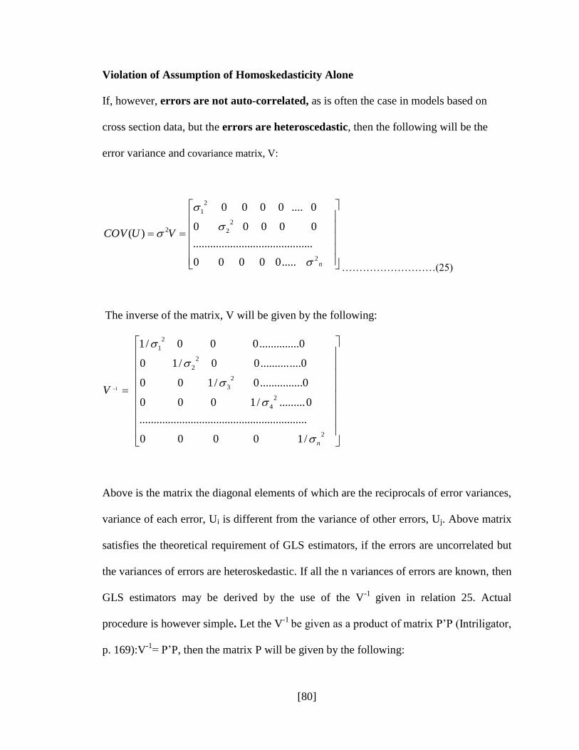
Violation of Assumption of Homoskedasticity Alone

If, however, errors are not auto-correlated, as is often the case in models based on

cross section data, but the errors are heteroscedastic, then the following will be the

error variance and covariance matrix, V:

n

VUCOV

2

2

2

2

1

2

.....00000

..........................................

00000

0....0000

)(

………………………(25)

The inverse of the matrix, V will be given by the following:

2

2

4

2

3

2

2

2

1

/10000

...........................................................

0........./1000

0...............0/100

0..............00/10

0..............000/1

1

n

V

Above is the matrix the diagonal elements of which are the reciprocals of error variances,

variance of each error, Ui is different from the variance of other errors, Uj. Above matrix

satisfies the theoretical requirement of GLS estimators, if the errors are uncorrelated but

the variances of errors are heteroskedastic. If all the n variances of errors are known, then

GLS estimators may be derived by the use of the V-1

given in relation 25. Actual

procedure is however simple. Let the V-1

be given as a product of matrix P’P (Intriligator,

p. 169):V-1

= P’P, then the matrix P will be given by the following:

[81]

2

2

4

2

3

2

2

2

1

/10000

...........................................................

0........./1000

0...............0/100

0..............00/10

0..............000/1

n

p

The original regression model Y=X’β+ U, be pre-multiplied by matrix P:

PY=P X’β+ PU,

Where error terms will satisfy the following conditions

E(PU)= PE(U)=0

E(PUP’U)=PE(UU’)P’= σ2

PVP’= σ2I ……………………………. (26)

This makes the procedure of GLS very simple in practice. OLS procedure is applied after

weighting each observation of dependent variable Y and independent variable (s) X, by

the corresponding reciprocal of the standard deviation of either the dependent variable or

reciprocal of the standard deviation of the random error. Therefore, the GLS may be

interpreted as estimation by OLS by the application of its procedure on the transformed

data base relating to Variables Y and X. The transformed vales of the variables will be as

follows:

PY= (Y1/σ1, Y2/σ3, Y3/σ3,…….., Yn/σn) and PX= (X1/σ1, X2/σ3, X3/σ3,……..,

Xn/σn)……(27)

14) Detection of Heteroscedastic

R.E. Park Test (1966) suggested that the error variances, σi2 may be regressed on one or

all predetermined variables of the regression model for testing Heteroscedasticity. Park

[82]

test is a special case of Harvey’ more general test of Heteroscedasticity. The model

suggested by Park is given below:

σi2= σ

2 Xi

α e

vi-------------------------------------------------------------(28)

Logarithmic transformation of above relation yields the following regression equation:

lnσi2= lnσ

2 + α1lnXi+vi-------------------------------------------------(29)

=0+1ln Xi+Vi

If 1 turns out to be statistically significant, it would suggest that hetroscedasticity is

present in the data. If it turns out to be in-significant , we may accept the assumption of

homoscedasticity.vi is the stochastic error term. Logarithmic transformation is needed for

transformation of exponential into linear function which may be estimated by OLS. As

σi2

is generally unknown, Park suggests the use of Ui2 as its proxy, while, lnσ

2 will

emerge as an estimate of the intercept of the function as a part of OLS estimators. If the

regression coefficient, α1 is statistically significant, then heteroscedasticity is serious, and

it needs remedial measures. If, however, α1 is not significant statistically, the hypothesis

of homoscedastic error variances may be accepted.

15) Cobweb Model

Cobweb Model is estimated by regressing Yt on time.

Yt=+1T------------------------------------------------------(30)

Where Yt shows difference between the highest and lowest prices of the week

(Amplitude) and T depicts time. Results highlight whether observed oscillations of prices

[83]

are damped (convergence towards stability). Explosive (volatile) or the amplitudes tend

towards constancy given by scalar-δ.

16) Simultaneous Equation Model

Simultaneous Equation Modeling is used to determine relation between five prices

reported in a day by stock exchange. Simultaneous equation models (SEMs), also called,

Structural equation models are multiple equation regression models. Unlike the more

traditional multivariate linear model, the response variable in one regression equation in

an SEM may appear as a predictor in another equation; indeed, variables in an SEM may

influence one-another reciprocally, either directly or through other variables as

intermediaries. These structural equations are meant to represent causal relationships

among the variables in the model. Single Equation Model comprises one equation alone

which is not supported by any conceptual, contextual and definitional relations. This

represents partial approach to analysis as such models assume, all factors and variables

other than those in the given equation as constant. There is only one single dependent

variable in the equation, the value of which is envisaged to be determined by one or more

than one independent variables. As against this, SEMs are self -contained. These models

represent general rather than partial approach to analysis, the model comprises two or

more equations and number of functional relations is equal to the number of jointly

related/dependent variable. Hence, one dependent variable corresponds to one

functional/regression analysis. Number of functional equations and number of dependent

relations are equal, though the total relations in the function are more than the number of

dependent variables. All the relations in the model define the structure and equations are

defined as structural equations. The number of structural equations in the system can be

[84]

reduced by linear combinations of two or more equations, since dependent variable in one

relation may appear as predetermined variable in the equation. Unknown coefficients are

estimated by reduced form parameters expressed in terms of structural parameters.

Number of such reduced form parameters and their equation should equal the number of

structural parameters to be determined by these equations. Otherwise one, some or all

may not be identifiable and hence cannot be estimated. Identification precedes

estimation.

Notation and Definitions: the general M equations model in MA endogenous, or jointly

dependent, variables may be written as

Y1t= β12Y2t+ β13Y3t+--------+ β1MYMT+λ11X1t + λ12X2t +-------+ λ1KXKt+U1t



-----------------------------------------------------------------------------------------------------------------------------------------------------------------

YMt= βM1Y1t+ βM2Y2t+--------+ βM,M-1YM-1,t+λM1X1t + λM2X2t +-------+ λMKXKt+UMt------(31)

Where Y1,Y2-----,YM= M endogenous , or jointly dependent, variables

X1,X2--------Xk= K predetermined variables (one of these X variables may take a value of

unity to allow for the intercept term in each equation)

U1, U2,------------UM=M stochastic disturbances

t=1,2,--------------------,T= total number of observations

β’s= coefficients of the endogenous variables

λ’s= coefficients of the predetermined variables

as equation (31) shows, the variables entering a Simultaneous-Equation model are of two

types : Endogenous, that is , those (whose values are ) determined within the model; and

Predetermined, that is, those (whose values are) determined outside the model. The

[85]

endogenous variables are regarded as stochastic, whereas the predetermined variables are

treated as non-stochastic.

Rules for Identification of ove-ridentified , exactly identified equations

To understand the order and rank conditions, following notations are introduced:

M=number of endogenous variables in the Model

(m) =number of endogenous variables in a given equation

K= number of predetermined variables in the model including in the intercept

(k)= number of predetermined variables in a given equation

1) In a model of M simultaneous equations in order for an equation to be identified, it

must excluded at least M-1 variables (endogenous as well as predetermined) appearing in

the model. If it excludes more than M-1 variables, it is over-identified.

2) In a model of M simultaneous equations, in order for an equation to be identified , the

number of predetermined variables excluded from the equation must not be less than the

number of endogenous variables included in that equation less 1 that is, K-k>m-1. If K-

k=m-1, the equation is just identified, but if K-k> m-1, it is over-identified.

The Rank Condition of identifiabilty: in a model containing M equations in M

endogenous variables, an equation is identified if and only if at least one nonzero

determinant of order (M-1) can be constructed from the coefficients of the variables

(both endogenous and predetermined) excluded from that particular equation but included

in the other equations of the model.

SEM formulated for jointly determined variables (Pct,Pot,Pht) on the basis of

predetermined variable (Pct-1, Pot-1, Pht-1, DV).

[86]

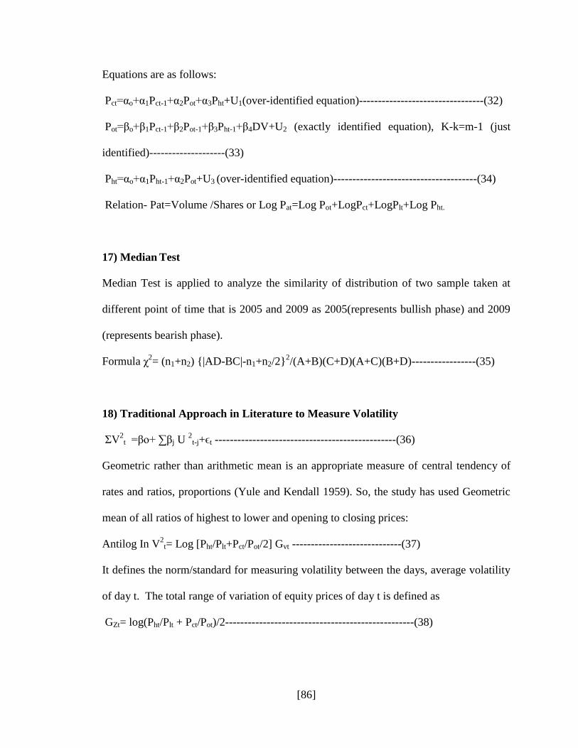
Equations are as follows:

Pct=αo+α1Pct-1+α2Pot+α3Pht+U1(over-identified equation)---------------------------------(32)

Pot=βo+β1Pct-1+β2Pot-1+β3Pht-1+β4DV+U2 (exactly identified equation), K-k=m-1 (just

identified)--------------------(33)

Pht=αo+α1Pht-1+α2Pot+U3 (over-identified equation)--------------------------------------(34)

Relation- Pat=Volume /Shares or Log Pat=Log Pot+LogPct+LogPlt+Log Pht.

17) Median Test

Median Test is applied to analyze the similarity of distribution of two sample taken at

different point of time that is 2005 and 2009 as 2005(represents bullish phase) and 2009

(represents bearish phase).

Formula χ2= (n1+n2) {|AD-BC|-n1+n2/2}

2/(A+B)(C+D)(A+C)(B+D)-----------------(35)

18) Traditional Approach in Literature to Measure Volatility

ΣV2

t =βo+ ∑βj U 2

t-j+ϵt ------------------------------------------------(36)

Geometric rather than arithmetic mean is an appropriate measure of central tendency of

rates and ratios, proportions (Yule and Kendall 1959). So, the study has used Geometric

mean of all ratios of highest to lower and opening to closing prices:

Antilog In V2

t= Log [Pht/Plt+Pct/Pot/2] Gvt -----------------------------(37)

It defines the norm/standard for measuring volatility between the days, average volatility

of day t. The total range of variation of equity prices of day t is defined as

GZt= log(Pht/Plt + Pct/Pot)/2--------------------------------------------------(38)

[87]

Above equation may be noted that the traditional proxy of volatility moderates the

variation by logarithmic transformation; it transforms non-linear into linear series.

19) ARCH (Autoregressive Conditional Hetroscedasticity) Model

ARCH Model is applied to measure the volatility.

In σV2 t=α0+α1InU

2t+α2In U

2t-1, -----------------------------------------------------------------------(39)

If δ<0, then ρ <1 extension of above model experimentation is done where stochastic

errors are considered as mirror image of systematic factor.

U 2 t=α0+ α1U

2t-1+V

2t +ϵt ----------------------------------------(40)

20) New Measurement of Volatility

The significance of volatile changes may be tested as follows

Z=|ϸ-P|/√PQ --------------------------------------------(41)

ϸ is proportion of sum of frequencies of values lying outside the defined range to all

observations in the study period, whereas P is the theoretical postulation of acceptable

range of M±σ . The significance of the difference between sample proposition ϸ and

expected proportion P is evaluated at 0.05 probability level. If such observations lie

outside M±σ, then distribution is treated as volatile. 95% of total observations lie within

the range of M±3 σ.

21) Chi-Square Test

Chi-Square test is a test of goodness of fit. It is applied in the study to find whether the

volatility index is a good fit normal curve.

[88]

χ2= ∑(z-ncz)

2/z------------------------------------------------------------(42)

Where z is volatility index and ncz is normalization of volatility Index.

3.3 Data Profile

Descriptive Statistics is applied to data to analyze the basic features of data. Nature

of distribution may be highlighted by the fact whether data approximates normal or non-

normal distribution. Since most of the statistical tests in parametric statistics assume the

distribution of values to be normal, an approximate measure of degree of divergence of

observed from normal distribution may be used Coefficients of variation, skewness and

kurtosis furnish an idea about departure from normality.in normal distribution mean,

median and mode are equal. So, significance of difference between mean and median is

also used as an indicator of departure from normality. Mean, median and mode coincide

in location in a normal distribution which is symmetrical about the mean/ median.

Become important. Values of most of these coefficients are reported under summary

statistics. The following are the formulae of these coefficients and measures:

3.3.1 Mean

Arithmetic average or mean is the simplest and most commonly used measure of central

tendency. Its most serious limitation is that it assigns weights to values in proportion to

their magnitudes which make the mean highly sensitive to the presence if extreme values

including outliers. Most commonly used procedure for its calculation is as follows:

M=∑(fiXi)/∑fi ……………….. (1)

[89]

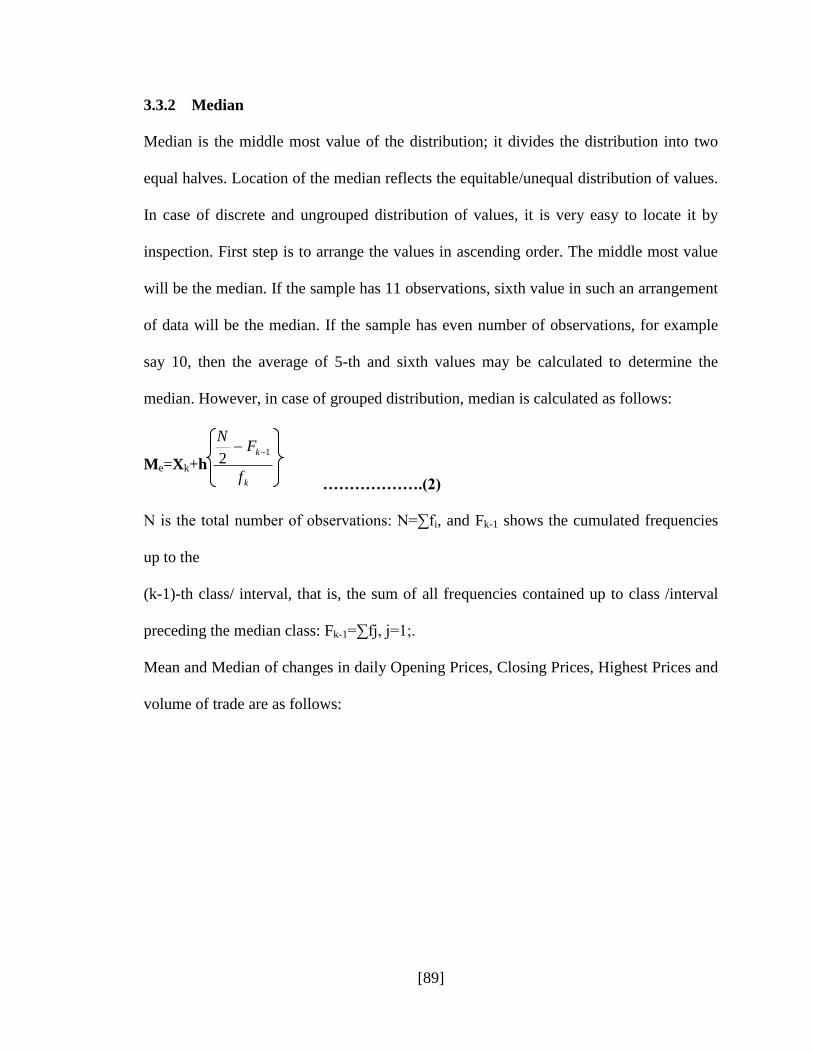
3.3.2 Median

Median is the middle most value of the distribution; it divides the distribution into two

equal halves. Location of the median reflects the equitable/unequal distribution of values.

In case of discrete and ungrouped distribution of values, it is very easy to locate it by

inspection. First step is to arrange the values in ascending order. The middle most value

will be the median. If the sample has 11 observations, sixth value in such an arrangement

of data will be the median. If the sample has even number of observations, for example

say 10, then the average of 5-th and sixth values may be calculated to determine the

median. However, in case of grouped distribution, median is calculated as follows:

Me=Xk+h k

k

f

FN

12

……………….(2)

N is the total number of observations: N=∑fi, and Fk-1 shows the cumulated frequencies

up to the

(k-1)-th class/ interval, that is, the sum of all frequencies contained up to class /interval

preceding the median class: Fk-1=∑fj, j=1;.

Mean and Median of changes in daily Opening Prices, Closing Prices, Highest Prices and

volume of trade are as follows:

[90]

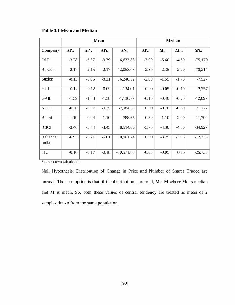
Table 3.1 Mean and Median

Mean Median

Company ΔPot ΔPct ΔPht ΔNst ΔPot ΔPct ΔPht ΔNst

DLF -3.28 -3.37 -3.39 16,633.83 -3.00 -5.60 -4.50 -75,170

RelCom -2.17 -2.15 -2.17 12,053.03 -2.30 -2.35 -2.70 -78,214

Suzlon -8.13 -8.05 -8.21 76,240.52 -2.00 -1.55 -1.75 -7,527

HUL 0.12 0.12 0.09 -134.01 0.00 -0.05 -0.10 2,757

GAIL -1.39 -1.33 -1.38 -1,136.79 -0.10 -0.40 -0.25 -12,097

NTPC -0.36 -0.37 -0.35 -2,984.38 0.00 -0.70 -0.60 71,227

Bharti -1.19 -0.94 -1.10 788.66 -0.30 -1.10 -2.00 11,794

ICICI -3.46 -3.44 -3.45 8,514.66 -3.70 -4.30 -4.00 -34,927

Reliance

India

-6.93 -6.21 -6.61 10,901.74 0.00 -3.25 -3.95 -12,335

ITC -0.16 -0.17 -0.18 -10,571.80 -0.05 -0.05 0.15 -25,735

Source : own calculation

Null Hypothesis: Distribution of Change in Price and Number of Shares Traded are

normal. The assumption is that ,if the distribution is normal, Me=M where Me is median

and M is mean. So, both these values of central tendency are treated as mean of 2

samples drawn from the same population.

[91]

Table : 3.2 t Value of Mean of differences on M and Me

Company ΔPot ΔPct ΔPht ΔNst

DLF -0.15064 1.30376 0.69583 1.51302

RelCom 0.09123 0.14648 0.46198 0.89201

Suzlon -0.89368 -0.98064 -0.94756 0.37470

HUL 0.29237 0.46581 0.66706 -0.06747

GAIL -1.19533 -0.96758 -1.23823 0.54773

NTPC -0.76399 0.76096 0.64434 -0.96772

Bharti -0.48043 0.09374 0.60303 -0.14391

ICICI 0.09553 0.39128 0.28636 0.60237

Reliance India -1.33183 -0.63186 -0.64421 0.62721

ITC -0.30663 -0.38438 -1.11828 0.22759


As all calculated values of t in the above table are less than 1.96, null hypotheses is

accepted that mean is approximately equal to median, which indicates that daily prices

and number of shares traded are normally distributed. This lends credence to the thesis

that prices are stable and do not embody volatility. Volatility is occasional in the market

and generally swing prices so, these results lend credence to the hypothesis in the prices

in a narrow band cannot be considered as volatility.

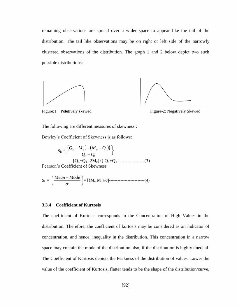
3.3.3 Coefficient of Skewness

Coefficient of Skewness is an important s calculated statistics for capturing an important

aspect of distribution of values. Coefficient of skewness shows clustering of some or few

high values in a narrow space; such observations make the curve of the distribution have

a ‘head with tail like shape’. Some observations are clustered in a narrow space and the

[92]

remaining observations are spread over a wider space to appear like the tail of the

distribution. The tail like observations may be on right or left side of the narrowly

clustered observations of the distribution. The graph 1 and 2 below depict two such

possible distributions:

Figure:1 Positively skewed Figure-2: Negatively Skewed

The following are different measures of skewness :

Bowley’s Coefficient of Skewness is as follows:

Sk =

= {Q3+Q1 -2Me}/{ Q3+Q1 } ……………(3)

Pearson’s Coefficient of Skewness

Sk = = [{Me- Mo}/σ]-------------------------(4)

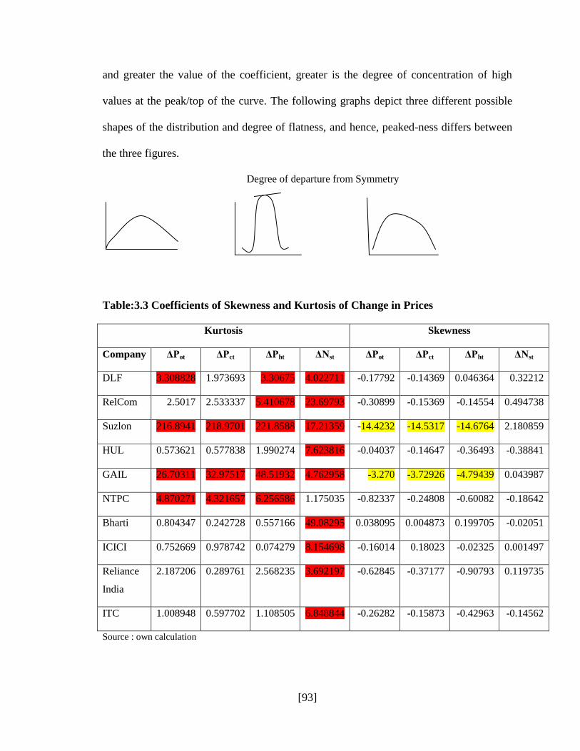
3.3.4 Coefficient of Kurtosis

The coefficient of Kurtosis corresponds to the Concentration of High Values in the

distribution. Therefore, the coefficient of kurtosis may be considered as an indicator of

concentration, and hence, inequality in the distribution. This concentration in a narrow

space may contain the mode of the distribution also, if the distribution is highly unequal.

The Coefficient of Kurtosis depicts the Peakness of the distribution of values. Lower the

value of the coefficient of Kurtosis, flatter tends to be the shape of the distribution/curve,

13

13

QQ

QMMQ ee

ModeMean

[93]

and greater the value of the coefficient, greater is the degree of concentration of high

values at the peak/top of the curve. The following graphs depict three different possible

shapes of the distribution and degree of flatness, and hence, peaked-ness differs between

the three figures.

Degree of departure from Symmetry

Table:3.3 Coefficients of Skewness and Kurtosis of Change in Prices

Kurtosis Skewness

Company ΔPot ΔPct ΔPht ΔNst ΔPot ΔPct ΔPht ΔNst

DLF 3.308828 1.973693 3.30675 4.022711 -0.17792 -0.14369 0.046364 0.32212

RelCom 2.5017 2.533337 5.410678 23.69793 -0.30899 -0.15369 -0.14554 0.494738

Suzlon 216.8941 218.9701 221.8588 17.21359 -14.4232 -14.5317 -14.6764 2.180859

HUL 0.573621 0.577838 1.990274 7.623816 -0.04037 -0.14647 -0.36493 -0.38841

GAIL 26.70311 32.97517 48.51932 4.762958 -3.270 -3.72926 -4.79439 0.043987

NTPC 4.870271 4.321657 6.256586 1.175035 -0.82337 -0.24808 -0.60082 -0.18642

Bharti 0.804347 0.242728 0.557166 49.08295 0.038095 0.004873 0.199705 -0.02051

ICICI 0.752669 0.978742 0.074279 8.154698 -0.16014 0.18023 -0.02325 0.001497

Reliance

India

2.187206 0.289761 2.568235 3.692197 -0.62845 -0.37177 -0.90793 0.119735

ITC 1.008948 0.597702 1.108505 6.848844 -0.26282 -0.15873 -0.42963 -0.14562


[94]

In the above table, the coefficient of skewness computed by Excel is given. Excel uses

Fisher –Pearson formula .Generally it lies between +1 and -1. In case of Fisher-Pearson

formula, the coefficient may vary around ±3. Changes in opening ,highest and closing

price of the day are moderately or highly skewed in case of Suzlon and GAIL. For both

companies, distribution is negatively skewed

In the above table it is observed that except for SUZLON and GAIL kurtosis of all

companies are moderate. Concentrations of high values in these companies indicates

concentration of high value over few days inequality. Which may reflect high price

oscillations and hence volatility.

3.3.5 Coefficient of Variation

CV=(σ/Mean)*100 coefficient of variation is useful when comparing the variability of

two or more data set. It is a relative measure of variation .It is expressed in percentage.

The table (3.7) calculated values of CV per day. This will provide the idea about

variation per day in the successive changes in the price.

[95]

Table: 3.4 Values are in Percentages

Companies ΔPot ΔPct ΔPht ΔNst

DLF -2.98 -3.12 -2.91 22.54

Rel Com -3.95 -3.77 -3.25 51.89

Suzlon -5.21 -5.09 -5.13 18.12

HUL 21.14 18.47 18.61 -1976.51

GAIL -4.80 -4.47 -4.09 -108.8

NTPC -8.09 -6.93 -6.83 -158.83

Bharti -9.6414 -10.6 -8.24 599.39

ICICI -4.33 -3.92 -3.41 52.35

Rel Ind -4.64 -4.66 -3.86 21

ITC -14.054 -11.51 -10 -38.95


The table shows (i) lower magnitudes of change in opening than closing prices of the

day;(ii) four companies, viz HUL, NTPC, Bharti and ITC have value of CV greater than

5%, infact , it ranges from (-8.09)-(-9.64) to (-24.05) to (21.14) % which is much greater

than the variation in opening prices of other six companies; (iii) lowest price of the day

shows highest percentage change for reasons that are obvious. Variations of lowest prices

of the day do qualify to be dubbed volatile; (iv) variation in closing and highest prices of

the day almost match each other.

The above table highlights the pattern of changes in the daily prices varies from a

minimum 2% to maximum21% per day. Closing price varies from a minimum 3% to

maximum 18%. Highest price varies from minimum 2.9% to maximum 18%. Range of

variation is high for opening price than closing and highest price. Whereas, the change in

variation per day of closing and highest price is more or less similar.

[96]

3.4 Graphs of change in daily price will help in capturing overall results for one year Table 3.5 Pattern of Change in Opening Price

Companies Pattern of change in opening prices of the companies

GAIL

Accelerated Rise

NTPC

Logistic Slow Rise

Bharti

Modest Rise

0.00%20.00%40.00%60.00%80.00%100.00%120.00%

020406080

100120

Freq

uency

Frequency

Cumulative %

0.00%20.00%40.00%60.00%80.00%100.00%120.00%

0

20

40

60

80

Freq

uency

Frequency

Cumulative %

0.00%50.00%100.00%150.00%

0204060

Freq

uency

Bin

Histogram

Frequency

Cumulative %

[97]

ICICI

Modest Rise

Rel Ind

Rapid Rise

ITC

Low Rise

0.00%50.00%100.00%150.00%

0204060

Freq

uency

Bin

Histogram

Frequency

Cumulative %

0.00%50.00%100.00%150.00%

0204060

Freq

uency

Bin

Histogram

Frequency

Cumulative %

0.00%50.00%100.00%150.00%

01020304050

‐23

‐17.74

‐12.48

‐7.22

‐1.96

3.3

8.56

13.82Freq

uency

Bin

Histogram

Frequency

Cumulative %

[98]

HUL

Very Low Rise

Suzlon

Share break from constant changes

RelCom

Rapid Rise

0.00%50.00%100.00%150.00%

0204060

Freq

uency

Bin

Histogram

Frequency

Cumulative %

0.00%50.00%100.00%150.00%

0100200300

Freq

uency

Bin

Histogram

Frequency

Cumulative %

0.00%20.00%40.00%60.00%80.00%100.00%120.00%

0102030405060

Freq

uency

Bin

Frequency

Cumulative %

[99]

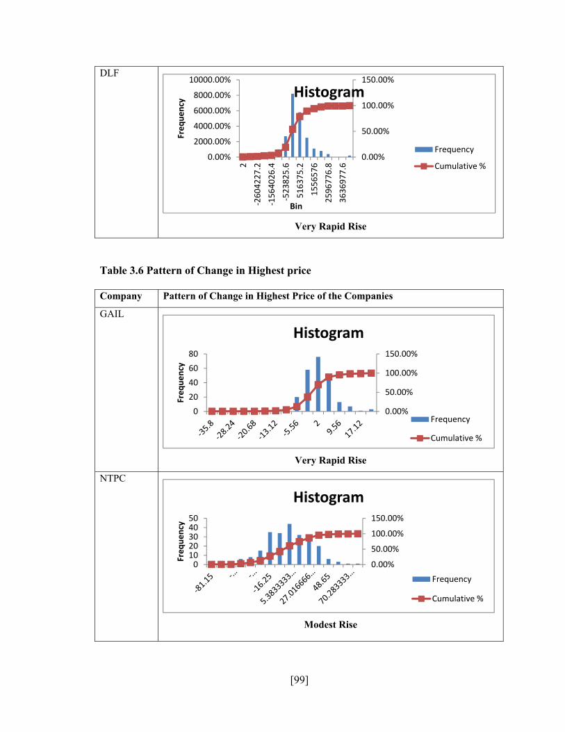
DLF

Very Rapid Rise

Table 3.6 Pattern of Change in Highest price

0.00%

50.00%

100.00%

150.00%

0.00%

2000.00%

4000.00%

6000.00%

8000.00%

10000.00%

2‐2604227.2

‐1564026.4

‐523825.6

516375.2

1556576

2596776.8

3636977.6

Freq

uency

Bin

Histogram

Frequency

Cumulative %

Company Pattern of Change in Highest Price of the Companies

GAIL

Very Rapid Rise

NTPC

Modest Rise

0.00%

50.00%

100.00%

150.00%

020406080

Freq

uency

Histogram

Frequency

Cumulative %

0.00%

50.00%

100.00%

150.00%

01020304050

Freq

uency

Histogram

Frequency

Cumulative %

[100]

Bharti

Modest Rise

ICICI

Modest Rise

Rel Ind

Modest Rise

0.00%

50.00%

100.00%

150.00%

010203040

Freq

uency

Histogram

Frequency

Cumulative %

0.00%

50.00%

100.00%

150.00%

0

20

40

60

Freq

uency

Histogram

Frequency

Cumulative %

0.00%

50.00%

100.00%

150.00%

01020304050

Freq

uency

Histogram

Frequency

Cumulative %

[101]

ITC

Modest Rise

HUL

Break in Constant Change

Suzlon

Modest Rise

0.00%

50.00%

100.00%

150.00%

020406080

Freq

uency

Histogram

Frequency

Cumulative %

0.00%

50.00%

100.00%

150.00%

050

100150200250

Freq

uency

Histogram

Frequency

Cumulative %

0.00%

50.00%

100.00%

150.00%

020406080

Freq

uency

Histogram

Frequency

Cumulative %

[102]

3.7 Pattern of Change in Closing Price Company Pattern of change in Closing Price of the Company

GAIL

Low Rise

0.00%

50.00%

100.00%

150.00%

0

50

100

150

Freq

uency

Histogram

Frequency

Cumulative %

RelCom

Modest Rise

DLF

Rapid Rise

0.00%

20.00%

40.00%

60.00%

80.00%

100.00%

120.00%

0

20

40

60

80

‐109.7 ‐… ‐…

‐67.56‐… ‐…

‐25.42‐…

2.673…

16.72

30.76…

44.81…

58.86

72.90…

86.95…

More

Freq

uency

Histogram Frequency

0.00%

50.00%

100.00%

150.00%

0

20

40

60

80

‐… ‐… ‐… ‐… ‐… ‐… ‐… ‐…2.67…

16.72

30.7…

44.8…

58.86

72.9…

86.9…

More

Freq

uency

Bin

Histogram

Frequency

Cumulative %

[103]

NTPC

Modest Rise

Bharti

Modest Rise

ICICI

Modest Rise

0.00%

50.00%

100.00%

150.00%

020406080

Freq

uency

Histogram

Frequency

Cumulative %

0.00%

50.00%

100.00%

150.00%

01020304050

Freq

uency

Histogram

Frequency

Cumulative %

0.00%20.00%40.00%60.00%80.00%100.00%120.00%

010203040

Freq

uency

Histogram

Frequency

Cumulative %

[104]

Rel Ind

Modest Rise

ITC

Modest Rise

HUL

Modest Rise

0.00%

50.00%

100.00%

150.00%

01020304050

Freq

uency

Histogram

Frequency

Cumulative %

0.00%50.00%100.00%150.00%

0204060

Freq

uency

Histogram

Frequency

Cumulative %

0.00%50.00%100.00%150.00%

01020304050

Freq

uency

modest rise

Histogram

Frequency

Cumulative %

[105]

Suzlon

Break in Constant Change

RelCom

Modest Rise

DLF

Steep Rise

Above Graphs partly trace the path of Logistic curve for all companies except Suzlon, it

is an approximation to normal curve for there is sharp decline in the price and then it

becomes constant subsequently. Prakash, Patel and Lamba, 2012) incidentally found

0.00%50.00%100.00%150.00%

0100200300

Freq

uency

Histogram

Frequency

Cumulative %

0.00%

50.00%

100.00%

150.00%

020406080

Freq

uency

Histogram

Frequency

Cumulative %

0.00%

20.00%

40.00%

60.00%

80.00%

100.00%

120.00%

0

10

20

30

40

50

60

‐… ‐… ‐…‐68.65‐… ‐…

‐31.35‐… ‐…

5.95

18.3…

30.8…

43.25

55.6…

68.1…

More

Freq

uency

Histogram Frequency

Cumulative %

[106]

Suzlon to be the most efficient company in BSE. The curve for Suzlon may indicate non-

normal distribution These graphs are of change in opening price, highest price and

closing price.

Above analysis has followed the lead of Osborne and Fama (1953, 1965) who observed

that behaviour of market can be captured by analysis of successive change in prices.

Curves above and descriptive statistics make this researcher thinks whether volatility

exists in daily prices. Results also suggest, reformulation and measurement of volatility

by an alternative method. Daily prices of one year show remarkable signs of stationarity.

Review of Literature on volatility has either considered daily spread of highest /lowest

price or opening /closing price or tried to capture volatility through monthly average

price. This study is an innovation where all prices in a day are considered to measure

volatility in the theoretical framework of Flex Price and Cob –Web Model.

Another feature of the curves is that Opening Prices of all ten Companies are different

from curves of other prices. Besides, highest and Closing Prices are, more or less, traced

by similar curves. If market sentiment is positive, opening price moves towards the

highest price of the day, which boost to closing price, if sentiment remains the same.

Each price, reported in the market builds sentiment for the day. This supports our

objective of analyzing Behaviour of five prices in a day reported by stock market. This

study may make a modest contribution to the knowledge of asset pricing.

[107]

3.5 Profile of Five Years Daily Data of Four Companies

Another aspect of the study is also to analyze the long run data of stock prices. This

further stimulates the inquisitiveness that arises in the mind of researcher in view of a

daily prices of ten companies of 2008 are almost normal. Question to whether these

tendencies of prices remain the same if the sample is increased from one year to five

years. Two new companies are added in the sample to broaden the base of findings.

Results of Descriptive Statistics of four companies daily prices of five years from 2005 to

2010 are as follows:

Table3.8 ∆Pot Changes in Opening Price

COMPANY MEAN MEDIAN STANDARD

DEVIATION

SKEWNESS KURTOSIS

INFOSYS -1.597 -0.55 41.04 0.37 4.52

RELIANCE

INDUSTRIES

-0.531 -1.00 26.62 0.31 17.97

NTPC -0.076 0.00 4.65 0.58 14.49

BHEL -0.263 -0.25 9.26 0.03 7.32


Above table depicts following results: (i) Standard deviation of changes in opening price

ranges from the minimum 4.65 to maximum 41.04 of daily five year prices which cannot

be considered high in view of the long period of 5 years for stock market . (ii) Skewness

ranges from 0.03 to 0.58, which is within range of ±3. This results that changes in

opening prices are almost equally distributed on both ends of the mean; (ii) Kurtosis

ranges from minimum 4.52 to maximum 17.97 , for all companies which can be

considered high, that is above 3.

[108]

Table 3.9:∆Pht Change in Highest Price


DEVIATION SKEWNESS KURTOSIS

INFOSYS -1.607 -1.000 34.251 0.115 5.601

RELIANCE

INDUSTRIES -0.534 -0.825 22.396 0.476 27.788

NTPC -0.076 0.050 3.720 0.098 12.595

BHEL -0.265 0.000 8.175 -2.008 25.980


Above results of highest price is as follows: (i) Standard Deviation ranges from minimum

3.72 to maximum 34.25. Standard deviation of highest price is higher for private

companies than for public companies;(ii) The distribution of changes in highest prices of

BHEL are negatively skewed but the distribution of other companies changes in highest

prices is lowly and positively skewed though it ranges within parameter (iii) Kurtosis

ranges from minimum 5.601 to maximum 27.788 that is above 3 which shows that the

coefficients of Kurtosis of distribution of highest prices of the day are high and positive.

Table 3.10: ∆Plt Changes in Lowest Prices


DEVIATION

SKEWNESS KURTOSIS

INFOSYS -1.585 -2.41 34.983 0.235 3.095

RELIANCE

INDUSTRIES -0.533 -1.00 23.547 0.852 16.220

NTPC -0.075 -0.15 4.117 0.536 19.010

BHEL -0.260 -0.39 8.332 0.189 7.493


[109]

Above results shows that: (i) Standard deviation ranges from minimum 4.117 to

maximum 34.983; (ii) lowest prices are positively skewed but the coefficient of Kurtosis

is high for Reliance Industries and NTPC.

Table 3.11 ∆Pct Changes in Closing Prices

COMPANY MEAN MEDIAN CV SKEWNESS KURTOSIS

INFOSYS -1.6037 -0.55 35.9543 -0.0685 1.9688

RELIANCE

INDUSTRIES -0.5287 -0.70 22.0289 -0.0789 8.6583

NTPC -0.0753 0.00 3.9170 0.0804 9.8383

BHEL -0.2590 -0.03 8.1600 -0.6891 8.1374


Closing price of the day determines return on shares. Study of change in closing price

helps in analyzing the behaviour of prices which reflect performance of companies in the

market.

Above results indicate that (i) Coefficient of Variation ranges from minimum 3.9170 for

NTPC to the maximum 35.9543 for Reliance Industries. This indicates low variation

over time but variation of changes in closing prices is quite high for Infosys and Reliance

India but low for NTPC and BHEL(ii) skewness of the companies approximately zero

(iii) Kurtosis of the company ranges from 1.9688 to 9.8383 which are high. It can be

observe that kurtosis of all companies are out of the range. The concentration of high

values this may lead to inequality.

[110]

3.6 Test of symmetry of Distribution

Null Hypothesis: Mean=Median (to test this hypothesis following test is applied)

Results of application of test for variation of prices from mean to median are given

below:

Table3.12 Result of t test

COMPANY ΔPot ΔPht ΔPlt ΔPct

INFOSYS -1.081 -0.481 1.072 -1.013

RELIANCE

INDUSTRIES -1.532 0.887 1.105 0.697

NTPC -0.076 -0.594 1.329 -0.075

BHEL 0.757 -0.265 1.522 -0.117


From the above table the inferences are drawn (i) t test indicate the difference between

mean and median to be significant. Hence, the values of null hypothesis is accepted that

mean and median of all the daily prices of five years coincide and hence the distribution

is more or less identical (ii) ΔPot, ΔPht ΔPlt and ΔPct are normally distributed in the long

run eliminating volatility in prices; (iii) Volatility may be considered as only a very short

run phenomenon.

Mean test on five years data of four companies: symmetrical or normal distributions are

characterized by the equality of mean median and mode. All three measures of central

tendency are located at the top of the distribution in the middle. Consequently, positive

are matched by negative changes with each other. Therefore, it is assumed that the

distributions of changes in all four prices are normally Therefore null hypothesis is

[111]

accepted. This rule out the possibility of volatile changes. The hypothesis is further

strengthened by results of CV and Skewness. The detail reports on Coefficient of

Variation are given in following table.

Table 3.13 Coefficient of Variation per Day in percentage :

COMPANY Pot Pht Plt Pct

INFOSYS -0.0142 - 0.0118 -0.012 -0.012

RELIANCE

INDUSTRIES -0.0278 -0.023 -0.024 -0.023

NTPC 0.0006 -0.0272 -0.030 -0.028

BHEL -0.0195 -0.017 -0.018 -0.017


5 *360=1800 days

Coefficient of variation per day ranges from the minimum of 0 to 3 percentage which is

low.

These results support Marshallian theory that in the long run, prices move towards

average price. This further encourages investigator to analyze that pattern of distribution

of different companies in different years. Stock market is dynamic as it operates in totally

different economic and political environment each year. This study has used data for two

years, that is 2005 and 2009. 2005 was considered as boom period ,whereas in 2009,

market faced slowdown due to subprime crisis. These external shocks affected the stock

market to a great extent.

[112]

3.7 Median Test

Null Hypothesis: Median of 2 years (2005 and 2009) price is the same. If the two sets of

prices for 2005 and 2009 represent same population their Medians, Mo and Mean should

be same: Me1=Me2= Me where Me denotes median of composite years combined, and 1

and 2 refer to 2005 and 2009 respectively. Results are reported in table 3.15

Table 3.14: Table of Chi Test

COMPANY

NAME

Infosys Reliance

Industries

NTPC BHEL

χ2 1963.145 472.3281 472.3281 472.3281


The table shows that the calculated value for chi square for all companies are far greater

than the table value 3.87 for one degree of freedom. Results show that (i) Median of two

different years having different economic scenarios are not the same. (ii) Prices behave in

different way in different phases of cycles.

There is ample evidence to support the hypothesis that changes in all daily prices are

normally distributed. This rules out the possibility of volatile changes. The hypothesis is

further strengthened by results of CV and Skewness . The results may also be taken to

support Famas hypothesis that market is likely to be efficient in long run though

inefficiency and volatile changes may characterize the market in the short run. The results

also support the Marshallian thesis that, in the long run changes in prices move around

the average price . Besides, this also supports Prakash Subramaniam hypothesis that

prices generally move in narrow band, big- bang changes being occasional occurences. It

is conclusively evident despite the market being imperfect and short run inefficiency of

its operation that in the long run market converges to efficiency.

part ii chapter iii descriptive analysis of data and...

Documents