part 1: counterfactual causality and empirical research … their core, these types of questions are...

Part 1: Counterfactual Causalityand Empirical Research in the

Social Sciences

1

Chapter 1

Introduction

Did mandatory busing programs in the 1970s increase the school achievement ofdisadvantaged minority youth? If so, how much of a gain was achieved? Doesobtaining a college degree increase an individual’s labor market earnings? Ifso, is this particular effect large relative to the earnings gains that could beachieved only through on-the-job training? Did the use of a butterfly ballot insome Florida counties in the 2000 presidential election cost Al Gore votes? If so,was the number of miscast votes sufficiently large to have altered the electionoutcome?

At their core, these types of questions are simple cause-and-effect questionsof the form, Does X cause Y ? If X causes Y , how large is the effect of X onY ? Is the size of this effect large relative to the effects of other causes of Y ?

Simple cause-and-effect questions are the motivation for much empirical workin the social sciences, even though definitive answers to cause-and-effect ques-tions may not always be possible to formulate given the constraints that socialscientists face in collecting data. Even so, there is reason for optimism aboutour current and future abilities to effectively address cause-and-effect questions.In the past three decades, a counterfactual model of causality has been devel-oped, and a unified framework for the prosecution of causal questions is nowavailable. With this book, we aim to convince more social scientists to applythis model to the core empirical questions of the social sciences.

In this introductory chapter, we provide a skeletal precis of the main fea-tures of the counterfactual model. We then offer a brief and selective historyof causal analysis in quantitatively oriented observational social science. Wedevelop some background on the examples that we will draw on throughoutthe book, concluding with an introduction to graphical causal models that alsoprovides a roadmap to the remaining chapters.

3

4 Chapter 1. Introduction

1.1 The Counterfactual Model for ObservationalData Analysis

With its origins in early work on experimental design by Neyman (1990 [1923],1935), Fisher (1935), Cochran and Cox (1950), Kempthorne (1952), and Cox(1958), the counterfactual model for causal analysis of observational data wasformalized in a series of papers by Donald Rubin (1974, 1977, 1978, 1980a,1981, 1986, 1990). In the statistics tradition, the model is often referred toas the potential outcomes framework, with reference to potential yields fromNeyman’s work in agricultural statistics (see Gelman and Meng 2004; Rubin2005). The counterfactual model also has roots in the economics literature (Roy1951; Quandt 1972), with important subsequent work by James Heckman (seeHeckman 1974, 1978, 1979, 1989, 1992, 2000), Charles Manski (1995, 2003), andothers. Here, the model is also frequently referred to as the potential outcomesframework. The model is now dominant in both statistics and economics, andit is being used with increasing frequency in sociology, psychology, and politicalscience.

A counterfactual account of causation also exists in philosophy, which beganwith the seminal 1973 article of David Lewis, titled “Causation.”1 It is relatedto the counterfactual model for observational data analysis that we will presentin this book, but the philosophical version, as implied by the title of Lewis’ orig-inal article, aims to be a general model of causality. As noted by the philoso-pher James Woodward in his 2003 book, Making Things Happen: A Theory ofCausal Explanation, the counterfactual approach to causality championed byLewis and his students has not been influenced to any substantial degree bythe potential outcomes version of counterfactual modeling that we will presentin this book. However, Woodward attempts to bring the potential outcomesliterature into dialogue with philosophical models of causality, in part by aug-menting the important recent work of the computer scientist Judea Pearl. Wewill also use Pearl’s work extensively in our presentation, drawing on his 2000book, Causality: Models, Reasoning, and Inference. We will discuss the broaderphilosophical literature in Chapters 8 and 10, as it does have some implicationsfor social science practice and the pursuit of explanation more generally.

1In this tradition, causality is defined with reference to counterfactual dependence (or, asis sometimes written, the “ancestral” to counterfactual dependence). Accordingly, and at therisk of a great deal of oversimplification, the counterfactual account in philosophy maintainsthat it is proper to declare that, for events c and e, c causes e if (1) c and e both occur and(2) if c had not occurred and all else remained the same, then e would not have occurred.The primary challenge of the approach is to define the counterfactual scenario in which c doesnot occur (which Lewis did by imagining a limited “divergence miracle” that prevents c fromoccurring in a closest possible hypothetical world where all else is the same except that c doesnot occur). The approach differs substantially from the regularity-based theories of causalitythat dominated metaphysics through the 1960s, based on relations of entailment from coveringlaw models. For a recent collection of essays in philosophy on counterfactuals and causation,see Collins, Hall, and Paul (2004).

1.1. The Counterfactual Model 5

The core of the counterfactual model for observational data analysis is sim-ple. Suppose that each individual in a population of interest can be exposedto two alternative states of a cause. Each state is characterized by a distinctset of conditions, exposure to which potentially affects an outcome of interest,such as labor market earnings or scores on a standardized mathematics test. Ifthe outcome is earnings, the population of interest could be adults between theages of 30 and 50, and the two states could be whether or not an individualhas obtained a college degree. Alternatively, if the outcome is a mathematicstest score, the population of interest could be high school seniors, and the twostates could be whether or not a student has taken a course in trigonometry.In the counterfactual tradition, these alternative causal states are referred toas alternative treatments. When only two treatments are considered, they arereferred to as treatment and control. Throughout this book, we will conform tothis convention.

The key assumption of the counterfactual framework is that each individualin the population of interest has a potential outcome under each treatment state,even though each individual can be observed in only one treatment state at anypoint in time. For example, for the causal effect of having a college degreerather than only a high school degree on subsequent earnings, adults who havecompleted high school degrees have theoretical what-if earnings under the state“have a college degree,” and adults who have completed college degrees havetheoretical what-if earnings under the state “have only a high school degree.”These what-if potential outcomes are counterfactual.

Formalizing this conceptualization for a two-state treatment, the potentialoutcomes of each individual are defined as the true values of the outcome ofinterest that would result from exposure to the alternative causal states. Thepotential outcomes of each individual i are y1

i and y0i , where the superscript

1 signifies the treatment state and the superscript 0 signifies the control state.Because both y1

i and y0i exist in theory for each individual, an individual-level

causal effect can be defined as some contrast between y1i and y0

i , usually thesimple difference y1

i − y0i . Because it is impossible to observe both y1

i and y0i for

any individual, causal effects cannot be observed or directly calculated at theindividual level.2

By necessity, a researcher must analyze an observed outcome variable Ythat takes on values yi for each individual i that are equal to y1

i for those inthe treatment state and y0

i for those in the control state. We usually refer tothose in the treatment state as the treatment group and those in the controlstate as the control group.3 Accordingly, y0

i is an unobservable counterfactual

2The only generally effective strategy for estimating individual-level causal effects is acrossover design, in which individuals are exposed to two alternative treatments in successionand with enough time elapsed in between exposures such that the effects of the cause havehad time to dissipate (see Rothman and Greenland 1998). Obviously, such a design can beattempted only when a researcher has control over the allocation of the treatments and onlywhen the treatment effects are sufficiently ephemeral. These conditions rarely exist for thecausal questions that concern social scientists.

3We assume that, for observational data analysis, an underlying causal exposure mechanismexists in the population, and thus the distribution of individuals across the treatment and


outcome for each individual i in the treatment group, and y1i is an unobservable

counterfactual outcome for each individual i in the control group.In the counterfactual modeling tradition, attention is focused on estimating

various average causal effects, by analysis of the values yi, for groups of indi-viduals defined by specific characteristics. To do so effectively, the process bywhich individuals of different types are exposed to the cause of interest mustbe modeled. Doing so involves introducing defendable assumptions that allowfor the estimation of the average unobservable counterfactual values for specificgroups of individuals. If the assumptions are defendable, and a suitable methodfor constructing an average contrast from the data is chosen, then an averagedifference in the values of yi can be given a causal interpretation.

1.2 Causal Analysis and ObservationalSocial Science

The challenges of using observational data to justify causal claims are con-siderable. In this section, we present a selective history of the literature onthese challenges, focusing on the varied history of the usage of experimentallanguage in observational social science. We will also consider the growth ofsurvey research and the shift toward outcome-equation-based motivations ofcausal analysis that led to the widespread usage of regression estimators. Manyuseful discussions of these developments exist, and our presentation here is notmeant to be complete.4 We review only the literature that is relevant for ex-plaining the connections between the counterfactual model and other traditionsof quantitatively oriented analysis that are of interest to us here. We return tothese issues again in Chapters 8 and 10.

1.2.1 Experimental Language in Observational SocialScience

Although the word experiment has a very broad definition, in the social sciencesit is most closely associated with randomized experimental designs, such asthe double-blind clinical trials that have revolutionized the biomedical sciencesand the routine small-scale experiments that psychology professors perform on

control states exists independently of the observation and sampling process. Accordingly, thetreatment and control groups exist in the population, even though we typically observe onlysamples of them in the observed data. We will not require that the labels “treatment group”and “control group” refer only to the observed treatment and control groups.

4For a more complete synthesis of the literature on causality in observational social science,see, for sociology, Berk (1988, 2004), Bollen (1989), Goldthorpe (2000), Lieberson (1985),Lieberson and Lynn (2002), Marini and Singer (1988), Singer and Marini (1987), Sobel (1995,1996, 2000), and Smith (1990, 2003). For economics, see Angrist and Krueger (1999), Heckman(2000, 2005), Moffitt (2003), Pratt and Schlaifer (1984), and Rosenzweig and Wolpin (2000).For political science, see Brady and Collier (2004), King, Keohane, and Verba (1994), andMahoney and Goertz (2006).

1.2. Causal Analysis 7

their own students.5 Randomized experiments have their origins in the work ofstatistician Ronald A. Fisher during the 1920s, which then diffused throughoutvarious research communities via his widely read 1935 book, The Design ofExperiments.

Statisticians David Cox and Nancy Reid (2000) offer a definition of an ex-periment that focuses on the investigator’s deliberate control and that allowsfor a clear juxtaposition with an observational study:

The word experiment is used in a quite precise sense to mean aninvestigation where the system under study is under the control ofthe investigator. This means that the individuals or material inves-tigated, the nature of the treatments or manipulations under studyand the measurement procedures used are all selected, in their im-portant features at least, by the investigator.

By contrast in an observational study some of these features, andin particular the allocation of individuals to treatment groups, areoutside the investigator’s control. (Cox and Reid 2000:1)

We will maintain this basic distinction throughout this book. We will arguein this section that the counterfactual model of causality that we introducedin the last section is valuable precisely because it helps researchers to stipulateassumptions, evaluate alternative data analysis techniques, and think carefullyabout the process of causal exposure. Its success is a direct result of its languageof potential outcomes, which permits the analyst to conceptualize observationalstudies as if they were experimental designs controlled by someone other thanthe researcher – quite often, the subjects of the research. In this section, we offera brief discussion of other important attempts to use experimental language inobservational social science and that succeeded to varying degrees.

Samuel A. Stouffer, the sociologist and pioneering public opinion survey an-alyst, argued that “the progress of social science depends on the development oflimited theories – of considerable but still limited generality – from which pre-diction can be made to new concrete instances” (Stouffer 1962[1948]:5). Stoufferargued that, when testing alternative ideas, “it is essential that we always keepin mind the model of a controlled experiment, even if in practice we may haveto deviate from an ideal model” (Stouffer 1950:356). He followed this practiceover his career, from his 1930 dissertation that compared experimental withcase study methods of investigating attitudes, to his leadership of the team thatproduced The American Soldier during World War II (see Stouffer 1949), andin his 1955 classic Communism, Conformity, and Civil Liberties.

On his death, and in celebration of a posthumous collection of his essays,Stouffer was praised for his career of survey research and attendant explana-tory success. The demographer Philip Hauser noted that Stouffer “had a hand

5The Oxford English Dictionary provides the scientific definition of experiment: “An actionor operation undertaken in order to discover something unknown, to test a hypothesis, orestablish or illustrate some known truth” and also provides source references from as early as1362.


in major developments in virtually every aspect of the sample survey – sam-pling procedures, problem definition, questionnaire design, field and operatingprocedures, and analytic methods” (Hauser 1962:333). Arnold Rose (1962:720)declared, “Probably no sociologist was so ingenious in manipulating data sta-tistically to determine whether one hypothesis or another could be consideredas verified.” And Herbert Hyman portrayed his method of tabular analysis incharming detail:

While the vitality with which he attacked a table had to be observedin action, the characteristic strategy he employed was so calculatingthat one can sense it from reading the many printed examples. . . .Multivariate analysis for him was almost a way of life. Starting witha simple cross-tabulation, the relationship observed was elaboratedby the introduction of a third variable or test factor, leading to aclarification of the original relationship. . . . But there was a specialflavor to the way Sam handled it. With him, the love of a tablewas undying. Three variables weren’t enough. Four, five, six, evenseven variables were introduced, until that simple thing of beauty,that original little table, became one of those monstrous creaturesat the first sight of which a timid student would fall out of love withour profession forever. (Hyman 1962:324-5)

Stouffer’s method was to conceive of the experiment that he wished he couldhave conducted and then to work backwards by stratifying a sample of the pop-ulation of interest into subgroups until he felt comfortable that the remainingdifferences in the outcome could no longer be easily attributed to systematicdifferences within the subgroups. He never lost sight of the population of inter-est, and he appears to have always regarded his straightforward conclusions asthe best among plausible answers. Thus, as he said, “Though we cannot alwaysdesign neat experiments when we want to, we can at least keep the experimentalmodel in front of our eyes and behave cautiously” (Stouffer 1950:359).

Not all attempts to incorporate experimental language into observationalsocial science were as well received. Most notably in sociology, F. Stuart Chapinhad earlier argued explicitly for an experimental orientation to nearly all ofsociological research, but while turning the definition of an experiment in adirection that agitated others. For Chapin, a valid experiment did not requirethat the researcher obtain control over the treatment to be evaluated, only thatobservation of a causal process be conducted in controlled conditions (see Chapin1932, 1947). He thus considered what he called “ex post facto experiments”to be the solution to the inferential problems of the social sciences, and headvocated matching designs to select subsets of seemingly equivalent individualsfrom those who were and were not exposed to the treatment of interest. In sodoing, however, he proposed to ignore the incomparable, unmatched individuals,thereby losing sight of the population that Stouffer the survey analyst alwayskept in the foreground.

Chapin thereby ran afoul of emergent techniques of statistical inference,and he suffered attacks from his natural allies in quantitative analysis. The


statistician Oscar Kempthorne, whose 1952 book The Design and Analysis ofExperiments would later became a classic, dismissed Chapin’s work completely.In a review of Chapin’s 1947 book, Experimental Designs in Sociological Re-search, Kempthorne wrote:

The usage of the word “experimental design” is well established bynow to mean a plan for performing a comparative experiment. Thisimplies that various treatments are actually applied by the investiga-tor and are not just treatments that happened to have been appliedto particular units for some reason, known or unknown, before the“experiment” was planned. This condition rules out practically all ofthe experiments and experimental designs discussed by the author.(Kempthorne 1948:491)

Chapin’s colleagues in sociology were often just as unforgiving. Nathan Keyfitz(1948:260), for example, chastised Chapin for ignoring the population of interestand accused him of using terms such as “experimental design” merely to “lendthe support of their prestige.”

In spite of the backlash against Chapin, in the end he has a recognizablelegacy in observational data analysis. The matching techniques he advocatedwill be discussed later in Chapter 4. They have been reborn in the new liter-ature, in part because the population of interest has been brought back to theforeground. But there is an even more direct legacy. Many of Chapin’s so-calledexperiments were soon taken up, elaborated, and analyzed by the psychologistDonald T. Campbell and his colleagues under the milder and more general nameof “quasi-experiments.”6

The first widely read presentation of the Campbell’s perspective emerged in1963 (see Campbell and Stanley 1966[1963]), in which quasi-experiments werediscussed alongside randomized and fully controlled experimental trials, withan evaluation of their relative strengths and weaknesses in alternative settings.In the subsequent decade, Campbell’s work with his colleagues moved closer to-ward observational research, culminating in the volume by Cook and Campbell(1979), Quasi-Experimentation: Design & Analysis Issues for Field Settings,wherein a whole menu of quasi-experiments was described and analyzed: fromthe sort of ex post case-control matching studies advocated by Chapin (but re-labelled more generally as nonequivalent group designs) to novel proposals forregression discontinuity and interrupted time series designs (which we will dis-cuss later in Chapter 9). For Cook and Campbell, the term quasi-experimentrefers to “experiments that have treatments, outcome measures, and experi-mental units, but do not use random assignment to create the comparisons

6In his first publication on quasi-experiments, Campbell (1957) aligned himself with Stouf-fer’s perspective on the utility of experimental language, and in particular Stouffer (1950).Chapin is treated roughly by Campbell and Stanley (1963:70), even though his ex post factodesign is identified as “one of the most extended efforts toward quasi-experimental design.”


from which treatment-caused change is inferred” (Cook and Campbell 1979:6).7

And, rather than advocate for a reorientation of a whole discipline as Chapinhad, they pitched the approach as a guide for field studies, especially programevaluation studies of controlled interventions. Nonetheless, the ideas were widelyinfluential throughout the social sciences, as they succeeded in bringing a tamedexperimental language to the foreground in a way that permitted broad assess-ments of the strengths and weaknesses of alternative study designs and dataanalysis techniques.

1.2.2 “The Age of Regression”

Even though the quasi-experiment tradition swept through the program evalua-tion community and gained many readers elsewhere, it lost out in both sociologyand economics to equation-based motivations of observational data analysis, un-der the influence of a new generation of econometricians, demographers, and sur-vey researchers who developed structural equation and path-model techniques.Many of the key methodological advances took place in the field of economics, asdiscussed by Goldberger (1972) and Heckman (2000), even though the biologistSewall Wright (1925, 1934) is credited with the early development of some ofthe specific techniques.

In the 1960s, structural equation models spread quickly from economicsthroughout the social sciences, moving first to sociology via Hubert Blalockand Otis Dudley Duncan, each of whom is usually credited with introducingthe techniques, respectively, via Blalock’s 1964 book Causal Inferences in Non-experimental Research and Duncan’s 1966 article, “Path Analysis: SociologicalExamples,” which was published as the lead article in that year’s American Jour-nal of Sociology. In both presentations, caution is stressed. Blalock discussescarefully the differences between randomized experiments and observational sur-vey research. Duncan states explicitly in his abstract that “Path analysis focuseson the problem of interpretation and does not purport to be a method for dis-covering causes,” and he concludes his article with a long quotation from SewallWright attesting to the same point.

A confluence of developments then pushed structural equations towardwidespread usage and then basic regression modeling toward near complete dom-inance of observational research in some areas of social science. In sociology, themost important impetus was the immediate substantive payoff to the techniques.The American Occupational Structure, which Duncan cowrote with Peter Blauand published in 1967, transformed scholarship on social stratification, offer-ing new decompositions of the putative causal effects of parental backgroundand individuals’ own characteristics on later educational and occupational

7Notice that Cook and Campbell’s definition of quasi-experiments here is, in fact, consistentwith the definition of an experiment laid out by Cox and Reid, which we cited earlier. Forthat definition of an experiment, control is essential but randomization is not. The text ofCook and Campbell (1979) equivocates somewhat on these issues, but it is clear that theirintent is to discuss controlled experiments in which randomization is not feasible and thatthey then label quasi-experiments.


attainment. Their book transformed a core subfield of the discipline of soci-ology, leading to major theoretical and methodological redirections of manyexisting lines of scholarship.8

In part because of this success, it appears undeniable that Blalock and Dun-can became, for a time, less cautious. Blalock had already shown a predilectiontoward slippage. When introducing regression equations in his 1964 book, spec-ified as Yi = a + bXi + ei, where X is the causal variable of interest and Y isthe outcome variable of interest, Blalock then states correctly and clearly:

What if there existed a major determinant of Y , not explicitly con-tained in the regression equation, which was in fact correlated withsome of the independent variables Xi? Clearly, it would be contribut-ing to the error term in a manner so as to make the errors system-atically related to these particular Xi. If we were in a position tobring this unknown variable into the regression equation, we wouldfind that at least some of the regression coefficients (slopes) wouldbe changed. This is obviously an unsatisfactory state of affairs, mak-ing it nearly impossible to state accurate scientific generalizations.(Blalock 1964:47)

But Blalock ends his book with a set of numbered conclusions, among whichcan be found a different characterization of the same issue. Instead, he impliesthat the goal of causal inference should not be sacrificed even when these sortsof assumptions are dubious:

We shall assume that error terms are uncorrelated with each otherand with any of the independent variables in a given equation . . .. In nonexperimental studies involving nonisolated systems, thiskind of assumption is likely to be unrealistic. This means that dis-turbing influences must be explicitly brought into the model. But atsome point one must stop and make the simplifying assumption thatvariables left out do not produce confounding influences. Otherwise,causal inferences cannot be made. (Blalock 1964:176)

Blalock then elevates regression models to high scientific status: “In causalanalyses our aim is to focus on causal laws as represented by regression equationsand their coefficients” (Blalock 1964:177). And he then offers the practical advicethat “The method for making causal inferences may be applied to models basedon a priori reasoning, or it may be used in exploratory fashion to arrive at modelswhich give closer and closer approximations to the data” (Blalock 1964:179).

Not only are these conclusions unclear – Should the exploration-augmentedmodel still be regarded as a causal model? – they misrepresent the first 171pages of Blalock’s own book, in which he stressed the importance of assumptionsgrounded in substantive theory and offered repeated discussion of the differences

8For example, compare the methods (and substantive motivations) in Sewell (1964), withits nonparametric table standardization techniques, to Sewell, Haller, and Portes (1969), withits path model of the entire stratification process.


between regression equations embedded in recursive path models and the sortsof randomized experiments that often yield more easily defendable causal infer-ences. They also misrepresent the closing pages of his book, in which he returnswith caution to argue that a researcher should remain flexible, report inferencesfrom multiple models, and give an accounting of exploratory outcomes.

Duncan’s record is less obviously equivocal, as he never failed to mentionthat assumptions about causal relationships must be grounded in theory andcannot be revealed by data. Yet, as Abbott (2001[1998]:115) notes, “Duncanwas explicit in [The American Occupational Structure] about the extreme as-sumptions necessary for the analysis, but repeatedly urged the reader to bearwith him while he tried something out to see what could be learned.” What Dun-can learned transformed the field, and it was thus hard to ignore the potentialpower of the techniques to move the literature.

Duncan’s 1975 methodological text, Introduction to Structural Equation Mod-els, is appropriately restrained, with many fine discussions that echo the cautionin the abstract of his 1966 article. Yet he encourages widespread applicationof regression techniques to estimate causal effects, and at times he leaves theimpression that researchers should just get on with it as he did in the TheAmerican Occupational Structure. For example, in his Chapter 8, titled “Spec-ification Error,” Duncan notes that “it would require no elaborate sophistry toshow that we will never have the ‘right’ model in any absolute sense” (Duncan1975:101). But he then continues:

As the term will be used here, analysis of specification error relatesto a rhetorical strategy in which we suggest a model as the “true”one for sake of argument, determine how our working model [themodel that has been estimated] differs from it and what the con-sequences of the difference(s) are, and thereby get some sense ofhow important the mistakes we will inevitably make may be. Some-times it is possible to secure genuine comfort by this route. (Duncan1975:101-2)

As is widely known, Duncan later criticized the widespread usage of regres-sion analysis and structural equation modeling more generally, both in his 1984book Notes on Social Measurement: Historical and Critical and in private com-munication in which he reminded many inside and outside of sociology of hislong-standing cautionary perspective (see Xie 2006).

Finally, the emergent ease with which regression models could be estimatedwith new computing power was important as well. No longer would Stoufferhave needed to concentrate on a seven-way cross tabulation. His descendantscould instead estimate and then interpret only a few estimated regression slopes,rather than attempt to make sense of the hundred or so cells that Stoufferoften generated by subdivision of the sample. Aage Sørensen has given themost memorable indictment of the consequences of this revolution in computingpower:

With the advent of the high-speed computer, we certainly couldstudy the relationships among many more variables than before.

1.3. Types of Examples Used Throughout the Book 13

More importantly, we could compute precise quantitative measuresof the strength of these relationships. The revolution in quantitativesociology was a revolution in statistical productivity. Social scien-tists could now calculate almost everything with little manual laborand in very short periods of time. Unfortunately, the sociologicalworkers involved in this revolution lost control of their ability to seethe relationship between theory and evidence. Sociologists becamealienated from their sociological species being. (Sørensen 1998:241)

As this quotation intimates, enthusiasm for regression approaches to causalinference had declined dramatically by the mid-1990s. Naive usage of regressionmodeling was blamed for nearly all the ills of sociology, everything from strippingtemporality, context, and the valuation of case study methodologies from themainstream (see Abbott 2001 for a collections of essays), the suppression ofattention to explanatory mechanisms (see Hedstrom 2005 and Goldthorpe 2001),the denial of causal complexity (see Ragin 1987, 2000), and the destruction ofmathematical sociology (Sørensen 1998).

It is unfair to lay so much at the feet of least squares formulas, and we willargue later that regression can be put to work quite sensibly in the pursuit ofcausal questions. However, the critique of practice is largely on target. Forcausal analysis, the rise of regression led to a focus on equations for outcomes,rather than careful thinking about how the data in hand differ from what wouldhave been generated by the ideal experiments one might wish to have conducted.This sacrifice of attention to experimental thinking might have been reasonable ifthe outcome-equation tradition had led researchers to specify and then carefullyinvestigate the plausibility of alternative explanatory mechanisms that generatethe outcomes of the equations. But, instead, it seems that researchers all toooften chose not to develop fully articulated mechanisms that generate outcomesand instead chose to simply act as if the regression equations somehow mimicappreciably well (by a process not amenable to much analysis) the experimentsthat researchers might otherwise have wished to undertake.

The counterfactual model for observational data analysis has achieved suc-cess in the past two decades in the social sciences because it brings experimentallanguage back into observational data analysis. But it does so in the way thatStouffer used it: as a framework in which to ask carefully constructed “what-if”questions that lay bare the limitations of observational data and the need toclearly articulate assumptions grounded in theory that is believable.

1.3 Types of Examples Used Throughout theBook

In this section, we offer background on the main substantive examples that wewill draw on throughout the book when discussing the methods and approachabstractly and then when demonstrating particular empirical analysis strategies.


1.3.1 Broad Examples from Sociology, Economics,and Political Science

We first outline three prominent classic examples that, in spite of their distinctdisciplinary origins, are related to each other: (1) the causal effects of familybackground and mental ability on educational attainment, (2) the causal effectsof educational attainment and mental ability on earnings, and (3) the causaleffects of family background, educational attainment, and earnings on politicalparticipation. These examples are classic and wide ranging, having been de-veloped, respectively, in the formative years of observational data analysis insociology, economics, and political science.

The Causal Effects of Family Background and Intelligenceon Educational Attainment

In the status attainment tradition in sociology, as pioneered by Blau and Dun-can (1967), family background and mental ability are considered to be ultimatecauses of educational attainment. This claim is grounded on the purported ex-istence of a specific causal mechanism that relates individuals’ expectations andaspirations for the future to the social contexts that generate them. This par-ticular explanation is most often identified with the Wisconsin model of statusattainment, which was based on early analyses of the Wisconsin LongitudinalSurvey (see Sewell, Haller, and Portes 1969; Sewell, Haller, and Ohlendorf 1970).

According to the original Wisconsin model, the joint effects of high schoolstudents’ family backgrounds and mental abilities on their eventual educationalattainments can be completely explained by the expectations that others hold ofthem. In particular, significant others – parents, teachers, and peers – define ex-pectations based on students’ family background and observable academic per-formance. Students then internalize the expectations crafted by their significantothers. In the process, the expectations become individuals’ own aspirations,which then compel achievement motivation.

The implicit theory of the Wisconsin model maintains that students arecompelled to follow their own aspirations. Accordingly, the model is powerfullysimple, as it implies that significant others can increase high school students’future educational attainments merely by increasing their own expectations ofthem.9 Critics of this status attainment perspective argued that structural con-straints embedded in the opportunity structure of society should be at the centerof all models of educational attainment, and hence that concepts such as aspi-rations and expectations offer little or no explanatory power. Pierre Bourdieu(1973) dismissed all work that asserts that associations between aspirations andattainments are causal. Rather, for Bourdieu, the unequal opportunity struc-tures of society “determine aspirations by determining the extent to which theycan be satisfied” (Bourdieu 1973:83). And, as such, aspirations have no au-tonomous explanatory power because they are nothing other than alternativeindicators of structural opportunities and resulting attainment.

9See Hauser, Warren, Huang, and Carter (2000) for the latest update of the original model.


The Causal Effects of Educational Attainment and Mental Ability onEarnings

The economic theory of human capital maintains that education has a causaleffect on the subsequent labor market earnings of individuals. The theory pre-supposes that educational training provides skills that increase the potentialproductivity of workers. Because productivity is prized in the labor market,firms are willing to pay educated workers more.

These claims are largely accepted within economics, but considerable debateremains over the size of the causal effect of education. In reflecting on the firstedition of his book, Human Capital, which was published in 1964, Gary Beckerwrote nearly 30 years later:

Education and training are the most important investments in hu-man capital. My book showed, and so have many other studiessince then, that high school and college education in the UnitedStates greatly raise a person’s income, even after netting out directand indirect costs of schooling, and after adjusting for the betterfamily backgrounds and greater abilities of more educated people.Similar evidence is now available for many points in time from overone hundred countries with different cultures and economic systems.(Becker 1993[1964]:17)

The complication, hinted at in this quotation, is that economists also acceptthat mental ability enhances productivity as well. Thus, because those withrelatively high ability are assumed to be more likely to obtain higher educationaldegrees, the highly educated are presumed to have higher innate ability andhigher natural rates of productivity. As a result, some portion of the purportedcausal effect of education on earnings may instead reflect innate ability ratherthan any productivity-enhancing skills provided by educational institutions (seeWillis and Rosen 1979). The degree of “ability bias” in standard estimates ofthe causal effect of education on earnings has remained one of the largest causalcontroversies in the social sciences since the 1970s (see Card 1999).

The Causal Effects of Family Background, Educational Attainment,and Earnings on Political Participation

The socioeconomic status model of political participation asserts that education,occupational attainment, and income predict strongly most measures of politicalparticipation (see Verba and Nie 1972). Critics of this model maintain insteadthat political interests and engagement determine political participation, andthese are merely correlated with the main dimensions of socioeconomic status.10

10This interest model of participation has an equally long lineage. Lazarsfeld, Berelson,and Gaudet (1955[1948]:157) write that, in their local sample, “the difference in deliberatenon-voting between people with more or less education can be completely accounted for bythe notion of interest.”


In other words, those who have a predilection to participate in politics are likelyto show commitment to other institutions, such as the educational system.

Verba, Schlozman, and Brady (1995) later elaborated the socioeconomic sta-tus model, focusing on the contingent causal processes that they argue generatepatterns of participation through the resources conferred by socioeconomic po-sition. They claim:

. . . interest, information, efficacy, and partisan intensity provide thedesire, knowledge, and self-assurance that impel people to be en-gaged by politics. But time, money, and skills provide the where-withal without which engagement is meaningless. It is not sufficientto know and care about politics. If wishes were resources, then beg-gars would participate. (Verba et al. 1995:355-6)

They reach this conclusion through a series of regression models that predictpolitical participation. They use temporal order to establish causal order, andthey then claim to eliminate alternative theories that emphasize political in-terests and engagement by showing that these variables have relatively weakpredictive power in their models.

Moreover, they identify education as the single strongest cause of politicalparticipation. Beyond generating the crucial resources of time, money, and civicskills, education shapes preadult experiences and transmits differences in familybackground (see Verba et al. 1995, Figure 15.1). Education emerges as themost powerful cause of engagement because it has the largest net associationwith measures of political participation.

Nie, Junn, and Stehlik-Barry (1996) then built on the models of Verba andhis colleagues, specifying in detail the causal pathways linking education to po-litical participation. For this work, the effects of education, family income, andoccupational prominence (again, the three basic dimensions of socioeconomicstatus) on voting frequency are mediated by verbal proficiency, organizationalmembership, and social network centrality. Nie et al. (1996:76) note that thesevariables “almost fully explain the original bivariate relationship between edu-cation and frequency of voting.”

Each of these first three examples, as noted earlier, is concerned with rela-tionships that unfold over the lifecourse of the majority of individuals in mostindustrialized societies. As such, these examples encompass some of the mostimportant substantive scholarship in sociology, economics, and political science.At the same time, however, they pose some fundamental challenges for causalanalysis: measurement complications and potential nonmanipulability of thecauses of interest. Each of these deserves some comment before the narrowerand less complicated examples that follow are introduced.

First, the purported causal variables in these models are highly abstractand internally heterogeneous. Consider the political science example. Polit-ical participation takes many forms, from volunteer work to financial givingand voting. Each of these, in turn, is itself heterogeneous, given that individ-uals can contribute episodically and vote in only some elections. Furthermore,


family background and socioeconomic status include at least three underlyingdimensions: family income, parental education, and occupational position. Butother dimensions of advantage, such as wealth and family structure, must alsobe considered, as these are thought to be determinants of both an individual’seducational attainment and also the resources that supposedly enable politicalparticipation.11

Scholars who pursue analysis of these causal effects must therefore devotesubstantial energy to the development of measurement scales. Although veryimportant to consider, in this book we will not discuss measurement issues sothat we can focus closely on causal effect estimation strategies. But, of course,it should always be remembered that, in the absence of agreement on issues ofhow to measure a cause, few causal controversies can be resolved, no matterwhat estimation strategy seems best to adopt.

Second, each of these examples concerns causal effects for individual char-acteristics that are not easily manipulable through external intervention. Or,more to the point, even when they are manipulable, any such induced variationmay differ fundamentally from the naturally occurring (or socially determined)variation with which the models are most directly concerned. For example,family background could be manipulated by somehow convincing a sample ofmiddle-class and working-class parents to exchange their children at particularwell-chosen ages, but the subsequent outcomes of this induced variation maynot correspond to the family background differences that the original modelsattempt to use as explanatory differences.

As we will discuss later, whether nonmanipulability of a cause presents achallenge to an observational data analyst is a topic of continuing debate in themethodological and philosophical literature. We will discuss this complication atseveral points in this book, including a section in the concluding chapter. But,given that the measurement and manipulability concerns of the three broadexamples of this section present challenges at some level, we also draw on morenarrow examples throughout the book, as we discuss in the next section. Forthese more recent and more narrow examples, measurement is generally lesscontroversial and potential manipulability is more plausible (and in some casesis completely straightforward).

1.3.2 Narrow and Specific Examples

Throughout the book, we will introduce recent specific examples, most of whichcan be considered more narrow causal effects that are closely related to thebroad causal relationships represented in the three examples presented in thelast section. These examples will include, for example, the causal effect ofeducation on mental ability, the causal effect of military service on earnings,and the causal effect of felon disenfranchisement on election outcomes. To givea sense of the general characteristics of these narrower examples, we describe in

11Moreover, education as a cause is somewhat ungainly as well. For economists who wish tostudy the effects of learned skills on labor market earnings, simple variables measuring yearsof education obtained are oversimplified representations of human capital.


the remainder of this section four examples that we will use at multiple pointsthroughout the book: (1) the causal effect of Catholic schooling on learning,(2) the causal effect of school vouchers on learning, (3) the causal effect ofmanpower training on earnings, and (4) the causal effect of alternative votingtechnology on valid voting.

The Causal Effect of Catholic Schooling on Learning

James S. Coleman and his colleagues presented evidence that Catholic schoolsare more effective than public schools in teaching mathematics and reading toequivalent students (see Coleman and Hoffer 1987; Coleman, Hoffer, and Kil-gore 1982; Hoffer, Greeley, and Coleman 1985). Their findings were challengedvigorously by other researchers who argued that public school students andCatholic school students are insufficiently comparable, even after adjustmentsfor family background and measured motivation to learn (see Alexander andPallas 1983, 1985; Murnane, Newstead, and Olsen 1985; Noell 1982; Willms1985; see Morgan 2001 for a summary of the debate). Although the challengeswere wide ranging, the most compelling argument raised (and that was foreseenby Coleman and his colleagues) was that students who are most likely to benefitfrom Catholic schooling are more likely to enroll in Catholic schools net of allobservable characteristics. Thus, self-selection on the causal effect itself maygenerate a mistakenly large apparent Catholic school effect. If students insteadwere assigned randomly to Catholic and public schools, both types of schoolswould be shown to be equally effective on average.

To address the possibility that self-selection dynamics create an illusoryCatholic school effect, a later wave of studies then assessed whether or notnaturally occurring experiments were available that could be used to more ef-fectively estimate the Catholic school effect. Using a variety of variables thatpredict Catholic school attendance (e.g., share of the local population that isCatholic) and putting forth arguments for why these variables do not directly de-termine achievement, Evans and Schwab (1995), Hoxby (1996), and Neal (1997)generated support for Coleman’s original conclusions.

The Causal Effect of School Vouchers on Learning

In response to a perceived crisis in public education in the United States, pol-icymakers have introduced publicly funded school choice programs into somemetropolitan areas in an effort to increase competition among schools on theassumption that competition will improve school performance and resulting stu-dent achievement (see Chubb and Moe 1990; see also Fuller and Elmore 1996).Although these school choice programs differ by school district, the prototypi-cal design is the following. A set number of $3000 tuition vouchers redeemableat private schools are made available to students resident in the public schooldistrict, and all parents are encouraged to apply for one of these vouchers. Thevouchers are then randomly assigned among those who apply. Students who


receive a voucher remain eligible to enroll in the public school to which theirresidence status entitles them. But they can choose to enroll in a private school.If they choose to do so, they hand over their $3000 voucher and pay any requiredtop-up fees to meet the private school tuition.

The causal effects of interest resulting from these programs are numerous.Typically, evaluators are interested in the achievement differences between thosewho attend private schools using vouchers and other suitable comparison groups.Most commonly, the comparison group is the group of voucher applicants wholost out in the lottery and ended up in public schools (see Howell and Peterson2002; Hoxby 2003; Ladd 2002; Neal 2002). And, even though these sorts ofcomparisons may seem entirely straightforward, the published literature showsthat considerable controversy surrounds how best to estimate these effects, es-pecially given the real-world complexity that confronts the implementation ofrandomization schemes (see Krueger and Zhu 2004; Peterson and Howell 2004).

For this example, other effects are of interest as well. A researcher mightwish to know how the achievement of students who applied for vouchers butdid not receive them changed in comparison with those who never applied forvouchers in the first place (as this would be crucial for understanding how theself-selecting group of voucher applicants may differ from other public schoolstudents). More broadly, a researcher might wish to know the expected achieve-ment gain that would be observed for a public school student who was randomlyassigned a voucher irrespective of the application process. This would necessi-tate altering the voucher assignment mechanism, and thus it has not been anobject of research. Finally, the market competition justification for creatingthese school choice policies implies that the achievement differences of primaryinterest are those among public school students who attend voucher-threatenedpublic schools (i.e., public schools that feel as if they are in competition withprivate schools but that did not feel as if they were in competition with privateschools before the voucher program was introduced).

The Causal Effect of Manpower Training on Earnings

The United States federal government has supported manpower training pro-grams for economically disadvantaged citizens for decades (see LaLonde 1995).Through a series of legislative renewals, these programs have evolved substan-tially, and program evaluations have become an important area of applied workin labor and public economics.

The services provided to trainees differ and include classroom-basedvocational education, remedial high school instruction leading to a generalequivalency degree, and on-the-job training (or retraining) for those programparticipants who have substantial prior work experience. Moreover, the typesof individuals served by these programs are heterogeneous, including ex-felons,welfare recipients, and workers displaced from jobs by foreign competition. Ac-cordingly, the causal effects of interest are heterogeneous, varying with individ-ual characteristics and the particular form of training provided.


Even so, some common challenges have emerged across most program evalu-ations. Ashenfelter (1978) discovered what has become known as “Ashenfelter’sdip,” concluding after his analysis of training program data that

. . . all of the trainee groups suffered unpredicted earnings declines inthe year prior to training. . . . This suggests that simple before andafter comparisons of trainee earnings may be seriously misleadingevidence. (Ashenfelter 1978:55)

Because trainees tend to have experienced a downward spiral in earnings justbefore receiving training, the wages of trainees would rise to some degree evenin the absence of any training. Ashenfelter and Card (1985) then pursuedmodels of these “mean reversion” dynamics, demonstrating that the size oftreatment effect estimates is a function of alternative assumptions about pre-training earnings trajectories. They called for the construction of randomizedfield trials to improve program evaluation.

LaLonde (1986) then used results from program outcomes for the NationalSupported Work (NSW) Demonstration, a program from the mid-1970s thatrandomly assigned subjects to alternative treatment conditions. LaLonde ar-gued that most of the econometric techniques used for similar program evalua-tions failed to match the experimental estimates generated by the NSW data.Since LaLonde’s 1986 paper, econometricians have continued to refine proce-dures for evaluating both experimental and nonexperimental data from trainingprograms, focusing in detail on how to model the training selection mechanism(see Heckman, LaLonde, and Smith 1999; Manski and Garfinkel 1992; Smithand Todd 2005).

The Causal Effect of Alternative Voting Technology on Valid Voting

For specific causal effects embedded in the larger political participation debates,we could focus on particular decision points – the effect of education on campaigncontributions, net of income, and so on. However, the politics literature isappealing in another respect: outcomes in the form of actual votes cast andsubsequent election victories. These generate finely articulated counterfactualscenarios.

In the contested 2000 presidential election in the United States, considerableattention focused on the effect of voting technology on the election outcome inFlorida. Wand et al. (2001) published a refined version of their analysis thatspread like wildfire on the Internet in the week following the presidential election.They asserted that

. . . the butterfly ballot used in Palm Beach County, Florida, in the2000 presidential election caused more than 2,000 Democratic votersto vote by mistake for Reform candidate Pat Buchanan, a numberlarger than George W. Bush’s certified margin of victory in Florida.(Wand et al. 2001:793)

1.4. Observational Data and Random-Sample Surveys 21

Reflecting on efforts to recount votes undertaken by various media outlets, Wandand his colleagues identify the crucial contribution of their analysis:

Our analysis answers a counterfactual question about voter inten-tions that such investigations [by media outlets of votes cast] can-not resolve. The inspections may clarify the number of voters whomarked their ballot in support of the various candidates, but theinspections cannot tell us how many voters marked their ballot fora candidate they did not intend to choose. (Wand et al. 2001:804)

Herron and Sekhon (2003) then examined invalid votes that resulted from over-votes (i.e., voting for more than one candidate), arguing that such overvotesfurther hurt Gore’s vote tally in two crucial Florida counties. Finally, Mebane(2004) then considered statewide voting patterns, arguing that if voters’ inten-tions had not been thwarted by technology, Gore would have won the Floridapresidential election by 30,000 votes. One particularly interesting feature of thisexample is that the precise causal effect of voting technology on votes is not ofinterest, only the extent to which such causal effects aggregate to produce anelection outcome inconsistent with the preferences of those who voted.

1.4 Observational Data and Random-SampleSurveys

When we discuss methods and examples throughout this book, we will usuallyassume that the data have been generated by a relatively large random-samplesurvey. We will also assume that the proportion and pattern of individualswho are exposed to the cause are fixed in the population by whatever processgenerates causal exposure.

We rely on the random-sample perspective because we feel it is the most nat-ural framing of these methods for the typical social scientist, even though manyof the classic applications and early methodological pieces in this literature donot reference random-sample surveys. For the examples just summarized, thefirst three have been examined primarily with random-sample survey data, butmany of the others have not. Some, such as the manpower training example,depart substantially from this sort of setup, as the study subjects for the treat-ment in that example are a nonrandom and heterogeneous collection of welfarerecipients, ex-felons, and displaced workers.12

12Partly for this reason, some of the recent literature (e.g., Imbens 2004) has made carefuldistinctions between the sample average treatment effect (SATE) and the population averagetreatment effect (PATE). In this book, we will focus most of our attention on the PATE (andother conditional PATEs). We will generally write under the implicit assumption that a well-defined population exists (generally a superpopulation with explicit characteristics) and thatthe available data are a random sample from this population. However, much of our treatmentof these topics could be rewritten without the large random-sample perspective and focusingonly on the average treatment effect within the sample in hand. Many articles in this tradi-tion of analysis adopt this alternative starting point (especially those relevant for small-scalestudies in epidemiology and biostatistics for which the “sample” is generated in such a way


Pinning down the exact consequences of the data generation and samplingscheme of each application is important for developing estimates of the expectedvariability of a causal effect estimate. We will therefore generally modify therandom-sampling background when discussing what is known about the ex-pected variability of the alternative estimators we will present. However, wefocus more in this book on parameter identification than on the expected vari-ability of an estimator in a finite sample, as we discuss in the next section.

In fact, as the reader will notice in subsequent chapters, we often assumethat the sample is infinite. This preposterous assumption is useful for presen-tation purposes because it simplifies matters greatly; we can then assume thatsampling error is zero and assert, for example, that the sample mean of an ob-served variable is equal to the population expectation of that variable. But thisassumption is also an indirect note of caution: It is meant to appear preposter-ous and unreasonable in order to reinforce the point that the consequences ofsampling error must always be considered in any empirical analysis.13

Moreover, we will also assume for our presentation that the variables in thedata are measured without error. This perfect measurement assumption is, ofcourse, also entirely unreasonable. But it is commonly invoked in discussionsof causality and in many, if not most, other methodological pieces. We willindicate in various places throughout the book when random measurement erroris especially problematic for the methods that we present. We leave it as self-evident that nonrandom measurement error can be debilitating for all methods.

1.5 Identification and Statistical Inference

In the social sciences, identification and statistical inference are usually consid-ered separately. In his 1995 book, Identification Problems in the Social Sciences,the economist Charles Manski writes:

. . . it is useful to separate the inferential problem into statistical andidentification components. Studies of identification seek to char-acterize the conclusions that could be drawn if one could use thesampling process to obtain an unlimited number of observations.Identification problems cannot be solved by gathering more of thesame kind of data. (Manski 1995:4)

He continues:

Empirical research must, of course, contend with statistical issues aswell as with identification problems. Nevertheless, the two types of

that a formal connection to a well-defined population is impossible). We discuss these issues insubstantial detail in Chapter 2, especially in the appendix on alternative population models.

13Because we will in these cases assume that the sample is infinite, we must then also assumethat the population is infinite. This assumption entails adoption of the superpopulationperspective from statistics (wherein the finite population from which the sample is drawn isregarded as one realization of a stochastic superpopulation). Even so, and as we will explainin Chapter 2, we will not clutter the text of the book by making fine distinctions between theobservable finite population and its more encompassing superpopulation.

1.5. Identification and Statistical Inference 23

inferential difficulties are sufficiently distinct for it to be fruitful tostudy them separately. The study of identification logically comesfirst. Negative identification findings imply that statistical inferenceis fruitless: it makes no sense to try to use a sample of finite size toinfer something that could not be learned even if a sample of infinitesize were available. Positive identification findings imply that oneshould go on to study the feasibility of statistical inference. (Manski1995:5)

In contrast, in his 2002 book, Observational Studies, the statistician PaulRosenbaum sees the distinction between identification and statistical inferenceas considerably less helpful:

The idea of identification draws a bright red line between two typesof problems. Is this red line useful? . . . In principle, in a problemthat is formally not identified, there may be quite a bit of informationabout β, perhaps enough for some particular practical decision . . . .Arguably, a bright red line relating assumptions to asymptotics isless interesting than an exact confidence interval describing whathas been learned from the evidence actually at hand. (Rosenbaum2002:185–6)

Rosenbaum’s objection to the bright red line of identification is issued in thecontext of analyzing a particular type of estimator – an instrumental variableestimator – that can offer an estimate of a formally identified parameter that isso noisy in a dataset of any finite size that one cannot possibly learn anythingfrom the estimate. However, an alternative estimator – usually a least squaresregression estimator in this context – that does not formally identify a param-eter because it remains asymptotically biased even in an infinite sample maynonetheless provide sufficiently systematic information so as to remain useful,especially if one has a sense from other aspects of the analysis of the likelydirection and size of the bias.

We accept Rosenbaum’s perspective; it is undeniable that an empirical re-searcher who forsakes all concern with statistical inference could be led astrayby considering only estimates that are formally identified. But, for this book,our perspective is closer to that of Manski, and we focus on identification prob-lems almost exclusively. Nonetheless, where we feel it is important, we will offerdiscussions of the relative efficiency of estimators, such as for matching estima-tors and instrumental variable estimators. And we will discuss the utility ofcomparing alternative estimators based on the criterion of mean-squared error.Our primary goal, however, remains the clear presentation of material that canhelp researchers to determine what assumptions must be maintained in order toidentify causal effects, as well as the selection of an appropriate technique thatcan be used to estimate an identified causal effect from a sample of sufficientsize under whatever assumptions are justified.


1.6 Causal Graphs as an Introductionto the Remainder of the Book

After introducing the main pieces of the counterfactual model in Chapter 2, wewill then present conditioning techniques for causal effect estimation in Part2 of the book. In Chapter 3, we will present a basic conditioning frameworkusing causal diagrams. Then, in Chapters 4 and 5, we will explain matchingand regression estimators, showing how they are complementary variants of amore general conditioning approach.

In Part 3 of the book, we will then make the transition from “easy” to“hard” instances of causal effect estimation, for which simple conditioning willnot suffice because relevant variables that determine causal exposure are notobserved. After presenting the general predicament in Chapter 6, we will thenoffer Chapters 7 through 9 on instrumental variable techniques, mechanism-based estimation of causal effects, and the usage of over-time data to estimatecausal effects.

Finally, in Chapter 10 we will provide a summary of some of the objectionsthat others have developed against the counterfactual model. And we will con-clude the book with a broad discussion of the complementary modes of causalinquiry that comprise causal effect estimation in observational social science.

In part because the detailed table of contents already gives an accurate ac-counting of the material that we will present in the remaining chapters, we willnot provide a set of detailed chapter summaries here. Instead, we will concludethis introductory chapter with three causal diagrams and the causal effect esti-mation strategies that they suggest. These graphs allow us to foreshadow manyof the specific causal effect estimation strategies that we will present later.

Because the remainder of the material in this chapter will be reintroducedand more fully explained later (primarily in Chapters 3, 6, and 8), it can beskipped now without consequence. However, our experience in teaching thismaterial suggests that many readers may benefit from a quick graphical intro-duction to the basic estimation techniques before considering the details of thecounterfactual framework for observational data analysis.

Graphical Representations of Causal Relationships

Judea Pearl (2000) has developed a general set of rules for representing causalrelationships with graph theory. We will provide a more complete introductionto Pearl’s graph-theoretic modeling of causal relationships in Chapter 3, butfor now we use the most intuitive pieces of his graphical apparatus with onlyminimal explanation. That these graphs are readily interpretable and provideinsight with little introduction is testament to the clarity of Pearl’s contributionto causal analysis.

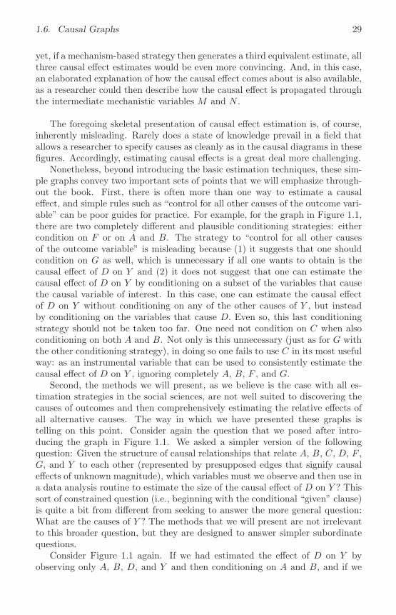
Consider the causal relationships depicted in the graph in Figure 1.1 andsuppose that these relationships are derived from a set of theoretical proposi-tions that have achieved consensus in the relevant scholarly community. For thisgraph, each node represents an observable random variable. Each directed edge

1.6. Causal Graphs 25

F G

D Y

A

C

B

Figure 1.1: A causal diagram in which back-door paths from D to Y can beblocked by observable variables and C is an instrumental variable for D.

(i.e., single-headed arrow) from one node to another signifies that the variableat the origin of the directed edge causes the variable at the terminus of the di-rected edge. Each curved and dashed bidirected edge (i.e., double-headed arrow)signifies the existence of common unobserved nodes that cause both terminalnodes. Bidirected edges represent common causes only, not mere correlationswith unknown sources and not relationships of direct causation between the twovariables that they connect.

Now, suppose that the causal variable of primary interest is D and that thecausal effect that we wish to estimate is the effect of D on Y . The question toconsider is the following: Given the structure of causal relationships representedin the graph, which variables must we observe and then use in a data analysisroutine to estimate the size of the causal effect of D on Y ?

Before answering this question, consider some of the finer points of the graph.In Pearl’s framework, the causal variable D has a probability distribution. Thecausal effects emanating from the variables A, B, and C are explicitly repre-sented in the graph by directed edges, but the relative sizes of these effects arenot represented in the graph. Other causes of D that are unrelated to A, B,and C are left implicit, as it is merely asserted in Pearl’s framework that D hasa probability distribution net of the systematic effects of A, B, and C on D.14

14There is considerable controversy over how to interpret these implicit causes. For some,the assertion of their existence is tantamount to asserting that causality is fundamentally prob-abilistic. For others, these implicit causes merely represent causes unrelated to the systematiccauses of interest. Under this interpretation, causality can still be considered a structural,deterministic relation. The latter position is closest to the position of Pearl (2000; see sections1.4 and 7.5).


The outcome variable, Y , is likewise caused by F , G, and D, but there are otherimplicit causes that are unrelated to F , G, and D that give Y its probabilitydistribution.

This graph is not a full causal model in Pearl’s framework because somesecond-order causes of D and Y create supplemental dependence between theobservable variables in the graph.15 These common causes are represented inthe graph by bidirected edges. In particular, A and B share some commoncauses that cannot be more finely specified by the state of knowledge in thefield. Likewise, A and F share some common causes that also cannot be morefinely specified by the state of knowledge in the field.

The Three Basic Strategies to Estimate Causal Effects

Three basic strategies for estimating causal effects will be covered in this book.First, one can condition on variables (with procedures such as stratification,matching, weighting, or regression) that block all back-door paths from thecausal variable to the outcome variable. Second, one can use exogenous varia-tion in an appropriate instrumental variable to isolate covariation in the causaland outcome variables. Third, one can establish an isolated and exhaustivemechanism that relates the causal variable to the outcome variable and thencalculate the causal effect as it propagates through the mechanism.

Consider the graph in Figure 1.1 and the opportunities it presents to estimatethe causal effect of D on Y with the conditioning estimation strategy. First notethat there are two back-door paths from D to Y in the graph that generate asupplemental noncausal association between D and Y : (1) D to A to F toY and (2) D to B to A to F to Y .16 Both of these back-door paths can beblocked in order to eliminate the supplemental noncausal association betweenD and Y by observing and then conditioning on A and B or by observing andthen conditioning on F . These two conditioning strategies are general in thesense that they will succeed in producing consistent causal effect estimates ofthe effect of D on Y under a variety of conditioning techniques and in thepresence of nonlinear effects. They are minimally sufficient in the sense thatone can observe and then condition on any subset of the observed variables in{A,B,C, F,G} as long as the subset includes either {A,B} or {F}.17

15Pearl would refer to this graph as a semi-Markovian causal diagram rather than a fullyMarkovian causal model (see Pearl 2000, Section 5.2).

16As we note later in Chapter 3 when more formally defining back-door paths, the two pathslabeled “back-door paths” in the main text here may represent many back-door paths becausethe bidirected edges may represent more than one common cause of the variables they pointto. Even so, the conclusions stated in the main text are unaffected by this possibility becausethe minimally sufficient conditioning strategies apply to all such additional back-door pathsas well.

17For the graph in Figure 1.1, one cannot effectively estimate the causal effect of D on Yby simply conditioning only on A. We explain this more completely in Chapter 3, where weintroduce the concept of a collider variable. The basic idea is that conditioning only on A,which is a collider, creates dependence between B and F within the strata of A. As a result,conditioning only on A fails to block all back-door paths from D to Y .


F G

H

D Y

A

B

C

Figure 1.2: A causal diagram in which C is no longer an instrumental variablefor D.

Now, consider the second estimation strategy, which is to use an instrumentalvariable for D to estimate the effect of D on Y . This strategy is completelydifferent from the conditioning strategy just summarized. The goal is not toblock back-door paths from the causal variable to the outcome variable butrather to use a localized exogenous shock to both the causal variable and theoutcome variable in order to estimate indirectly the relationship between thetwo. For the graph in Figure 1.1, the variable C is a valid instrument for Dbecause it causes D but does not have an effect on Y except though its effecton D. As a result, one can estimate consistently the causal effect of D on Y bytaking the ratio of the relationships between C and Y and between C and D.18

For this estimation strategy, A, B, F , and G do not need to be observed if theonly interest of a researcher is the causal effect of D on Y .

To further consider the differences between these first two strategies, nowconsider the alternative graph presented in Figure 1.2. There are five possiblestrategies for estimating the causal effect of D on Y for this graph, and theydiffer from those for the set of causal relationships in Figure 1.1 because a thirdback-door path is now present: D to C to H to Y . For the first four strategies,all back-door paths can be blocked by conditioning on {A,B,C}, {A,B,H},

18Although all other claims in this section hold for all distributions of the random variablesand all types of nonlinearity of causal relationships, one must assume for IV estimation whatPearl labels a linearity assumption. What this assumption means depends on the assumeddistribution of the variables. It would be satisfied if the causal effect of C on D is linear andthe causal effect of D on Y is linear. Both of these would be true, for example, if both C andD were binary variables and Y were an interval-scaled variable, and this is the most commonscenario we will consider in this book.


F G

M

D Y

A

C

B

N

Figure 1.3: A causal diagram in which M and N represent an isolated andexhaustive mechanism for the causal effect of D on Y .

{F, C}, or {F, H}. For the fifth strategy, the causal effect can be estimated byconditioning on H and then using C as an instrumental variable for D.

Finally, to see how the third mechanistic estimation strategy can be usedeffectively, consider the alternative graph presented in Figure 1.3. For thisgraph, four feasible strategies are available as well. The same three strategiesproposed for the graph in Figure 1.1 can be used. But, because the mediatingvariables M and N completely account for the causal effect of D on Y , andbecause M and N are not determined by anything other than D, the causaleffect of D on Y can also be calculated by estimation of the causal effect of Don M and N and then subsequently the causal effects of M and N on Y. And,because this strategy is available, if the goal is to obtain the causal effect of Don Y , then the variables A, B, C, F , and G can be ignored.19

In an ideal scenario, all three of these forms of causal effect estimation couldbe used to obtain estimates, and all three would generate equivalent estimates(subject to the expected variation produced by a finite sample from a popula-tion). If a causal effect estimate generated by conditioning on variables thatblock all back-door paths is similar to a causal effect estimate generated by avalid instrumental variable estimator, then each estimate is bolstered.20 Better

19Note that, for the graph in Figure 1.3, both M and N must be observed. If, instead, onlyM were observed, then this mechanistic estimation strategy will not identify the full causaleffect of D on Y . However, if M and N are isolated from each other, as they are in Figure 1.3,the portion of the causal effect that passes through M or N can be identified in the absenceof observation of the other. We discuss these issues in detail in Chapters 6 and 8.

20As we discuss in detail in Chapter 7, estimates generated by conditioning techniques andby valid instrumental variables will rarely be equivalent when individual-level heterogeneityof the causal effect is present (even in an infinite sample).


yet, if a mechanism-based strategy then generates a third equivalent estimate, allthree causal effect estimates would be even more convincing. And, in this case,an elaborated explanation of how the causal effect comes about is also available,as a researcher could then describe how the causal effect is propagated throughthe intermediate mechanistic variables M and N .

The foregoing skeletal presentation of causal effect estimation is, of course,inherently misleading. Rarely does a state of knowledge prevail in a field thatallows a researcher to specify causes as cleanly as in the causal diagrams in thesefigures. Accordingly, estimating causal effects is a great deal more challenging.

Nonetheless, beyond introducing the basic estimation techniques, these sim-ple graphs convey two important sets of points that we will emphasize through-out the book. First, there is often more than one way to estimate a causaleffect, and simple rules such as “control for all other causes of the outcome vari-able” can be poor guides for practice. For example, for the graph in Figure 1.1,there are two completely different and plausible conditioning strategies: eithercondition on F or on A and B. The strategy to “control for all other causesof the outcome variable” is misleading because (1) it suggests that one shouldcondition on G as well, which is unnecessary if all one wants to obtain is thecausal effect of D on Y and (2) it does not suggest that one can estimate thecausal effect of D on Y by conditioning on a subset of the variables that causethe causal variable of interest. In this case, one can estimate the causal effectof D on Y without conditioning on any of the other causes of Y , but insteadby conditioning on the variables that cause D. Even so, this last conditioningstrategy should not be taken too far. One need not condition on C when alsoconditioning on both A and B. Not only is this unnecessary (just as for G withthe other conditioning strategy), in doing so one fails to use C in its most usefulway: as an instrumental variable that can be used to consistently estimate thecausal effect of D on Y , ignoring completely A, B, F , and G.

Second, the methods we will present, as we believe is the case with all es-timation strategies in the social sciences, are not well suited to discovering thecauses of outcomes and then comprehensively estimating the relative effects ofall alternative causes. The way in which we have presented these graphs istelling on this point. Consider again the question that we posed after intro-ducing the graph in Figure 1.1. We asked a simpler version of the followingquestion: Given the structure of causal relationships that relate A, B, C, D, F ,G, and Y to each other (represented by presupposed edges that signify causaleffects of unknown magnitude), which variables must we observe and then use ina data analysis routine to estimate the size of the causal effect of D on Y ? Thissort of constrained question (i.e., beginning with the conditional “given” clause)is quite a bit from different from seeking to answer the more general question:What are the causes of Y ? The methods that we will present are not irrelevantto this broader question, but they are designed to answer simpler subordinatequestions.

Consider Figure 1.1 again. If we had estimated the effect of D on Y byobserving only A, B, D, and Y and then conditioning on A and B, and if we


then found that D had a trivially small effect on Y , we would then want toobserve both F and G and think further about whether what we considered tobe common causes of both A and F might be known and observable after all.However, if we did not have a theory and its associated state of knowledge thatsuggested that F and G have causal effects on Y (i.e., and instead thought thatD was the only systematic cause of Y ), then determining that D has a small tononexistent effect on Y would not help us to find any of the other causes of Ythat may be important.

The limited nature of the methods that we will present implies two importantfeatures of causal effect estimation from the perspective of counterfactual mod-eling. To offer a precise and defendable causal effect estimate, a well-specifiedtheory is needed to justify assumptions about underlying causal relationships.And, if theory is poorly specified, or divergent theories exist in the relevant schol-arly community that support alternative assumptions about underlying causalrelationships, then alternative causal effect estimates may be considered validconditional on the validity of alternative maintained assumptions. We discussthese issues in depth in the concluding section of the book, after presenting theframework and the methods that generate estimates that must then be placedin their proper context.

Chapter 2

The Counterfactual Model

In this chapter, we introduce the foundational components of the counterfactualmodel of causality, which is also known as the potential outcome model. Wefirst discuss causal states and the relationship between potential and observedoutcome variables. Then we introduce average causal effects and discuss theassumption of causal effect stability, which is maintained in most applicationsof the counterfactual model. We conclude with a discussion of simple estimationtechniques, in which we demonstrate the importance of considering the relation-ship between the potential outcomes and the process of causal exposure.

2.1 Causal States and Potential Outcomes

For a binary cause, the counterfactual framework presupposes the existenceof two well-defined causal states to which all members of the population ofinterest could be exposed.1 These two states are usually labeled treatment andcontrol. When a many-valued cause is analyzed, the convention is to refer tothe alternative states as alternative treatments.

Consider the examples introduced in Section 1.3. Some of these exampleshave well-defined states, and others do not. The manpower training exampleis completely straightforward, and the two states are whether an individual isenrolled in a training program or not. The Catholic school example is simi-lar. Here, the alternative states are “Catholic school” and “public school.” Theonly complication with these examples is the possibility of inherent differencesacross training programs and Catholic schools. If any such treatment-site het-erogeneity exists, then stratified analyses may be necessary, perhaps by regions

1We justify the importance of carefully defining the boundaries of the population of interestwhen presenting average causal effects later in this chapter. As we note there, we also providean appendix to this chapter, in which we explain the general superpopulation model that wewill adopt when the boundaries of the population can be clearly defined and when we havethe good fortune of having a large random sample from the population.

31

32 Chapter 2. The Counterfactual Model

of the country, size of the program, or whatever other dimension suggests thatvariability of the causal states deserves explicit modeling.2

Other examples have less clearly defined causal states. Consider the classicpolitical participation line of inquiry. For the relationship between socioeco-nomic status and political participation, there are many underlying well-definedcausal effects, such as the effect of having obtained at least a college degree onthe frequency of voting in local elections and the effect of having a family incomegreater than some cutoff value on the amount of money donated to political cam-paigns. Well-defined causal states exist for these narrow causal effects, but it isnot clear at all that well-defined causal states exist for the broad and internallydifferentiated concepts of socioeconomic status and political participation.

Finally, consider a related political science example. Beyond the votingtechnology effect discussed in Subsection 1.3.2 on the outcome of the 2000 pres-idential election, a broader set of question has been asked. To what extent dorestrictions on who can vote determine who wins elections? A recent and highlypublicized variant of this question is this: What is the effect on election outcomesof laws that forbid individuals with felony convictions from voting?3 Uggenand Manza (2002) make the straightforward claim that the 2000 presidentialelection would have gone in favor of Al Gore if felons and ex-felons had beenpermitted to vote:

Although the outcome of the extraordinarily close 2000 presiden-tial election could have been altered by a large number of factors, itwould almost certainly have been reversed had voting rights been ex-tended to any category of disenfranchised felons. (Uggen and Manza2002:792)

Uggen and Manza (2002) then note an important limitation of their conclusion:

. . . our counterfactual examples rely upon a ceteris paribus assump-tion – that nothing else about the candidates or election wouldchange save the voting rights of felons and ex-felons. (Uggen andManza 2002:795)

When thinking about this important qualification, one might surmise that apossible world in which felons had the right to vote would probably also be aworld in which the issues (and probably candidates) of the election would bevery different. Thus, the most challenging definitional issue here is not whocounts as a felon or whether or not an individual is disenfranchised, but ratherhow well the alternative causal states can be characterized.

As this example illustrates, it is important that the “what would have been”nature of the conditionals that define the causal states of interest be carefully

2Hong and Raudenbush (2006) provide a careful analysis of retention policies in U.S. pri-mary education, implementing this type of treatment-site stratification based on the averagelevel of retention in different schools.

3Behrens, Uggen, and Manza (2003), Manza and Uggen (2004), and Uggen, Behrens, andManza (2005) give historical perspective on this question.

2.1. Causal States and Potential Outcomes 33

laid out. When a ceteris paribus assumption is relied on to rule out othercontrasts that are nearly certain to occur at the same time, the posited causalstates are open to the charge that they are too metaphysical to justify thepursuit of causal analysis.4

Given the existence of well-defined causal states, causal inference in thecounterfactual tradition proceeds by stipulating the existence of potential out-come random variables that are defined over all individuals in the population ofinterest. For a binary cause, we will denote potential outcome random variablesas Y 1 and Y 0.5 We will also adopt the notational convention from statisticsin which realized values for random variables are denoted by lowercase letters.Accordingly, y1

i is the potential outcome in the treatment state for individuali, and y0

i is the potential outcome in the control state for individual i. Theindividual-level causal effect of the treatment is then defined as

δi = y1i − y0

i . (2.1)

Individual-level causal effects can be defined in ways other than as a linear dif-ference in the potential outcomes. For example, the individual-level causal effectcould be defined instead as the ratio of one individual-level potential outcometo another, as in y1

i /y0i . In some applications, there may be advantages to

these sorts of alternative definitions at the individual level, but the overwhelm-ing majority of the literature represents individual-level causal effects as lineardifferences, as in Equation (2.1).6

4This may well be the case with the felon disenfranchisement example, but this is a matterfor scholars in political sociology and criminology to debate. Even if the charge sticks, thisparticular line of research is nonetheless still an important contribution to the empirical liter-ature on how changing laws to allow felons and ex-felons to vote could have potential effectson election outcomes.

5There is a wide variety of notation in the potential outcome and counterfactuals literature,and we have adopted the notation that we feel is the easiest to grasp. However, we should notethat Equation (2.1) and its elements are often written as one of the following alternatives:

∆i = Y1i − Y0i ,

δi = Y ti − Y c

i ,

τ i = yi(1) − yi(0),

and variants thereof. We use the right-hand superscript to denote the potential treatmentstate of the corresponding potential outcome variable, but other authors use the right-handsubscript or parenthetical notation. We also use numerical values to refer to the treatmentstates, but other authors (including us, see Morgan 2001, Winship and Morgan 1999, andWinship and Sobel 2004) use values such as t and c for the treatment and control states,respectively. There is also variation in the usage of uppercase and lowercase letters. We donot claim that everyone will agree that our notation is the easiest to grasp, and it is certainlynot as general as, for example, the parenthetic notation. But it does seem to have provenitself in our own classes, offering the right balance between specificity and compactness.

6Moreover, the individual-level causal effect could be defined as the difference betweenthe expectations of individual-specific random variables, as in E[Y 1

i ] − E[Y 0i ], where E[.] is

the expectation operator from probability theory (see, for a clear example of this alternativesetup, King et al. 1994:76-82). In thinking about individuals self-selecting into alternativetreatment states, it can be useful to set up the treatment effects in this way. In many ap-plications, individuals are thought to consider potential outcomes with some recognition of


2.2 Treatment Groups and Observed Outcomes

For a binary cause with two causal states and associated potential outcomevariables Y 1 and Y 0, the convention in the counterfactuals literature is to definea causal exposure variable, D, which takes on two values: D is equal to 1 formembers of population who are exposed to the treatment state and equal to 0for members of the population who are exposed to the control state. Exposure tothe alternative causal states is determined by a particular process, typically anindividuals’s decision to enter one state or another, an outside actor’s decisionto allocate individuals to one state or another, a planned random allocationcarried out by an investigator, or some combination of these alternatives.

By convention, those who are exposed to the treatment state are referredto as the treatment group whereas those who are exposed to the control stateare referred to as the control group. Because D is defined as a population-level random variable (at least in most cases in observational data analysis), thetreatment group and control group exist in the population as well as the observeddata. Throughout this book, we will use this standard terminology, referringto treatment and control groups when discussing those who are exposed toalternative states of a binary cause. If more than two causal states are of interest,then we will shift to the semantics of alternative treatments and correspondingtreatment groups, thereby discarding the baseline labels of control state andcontrol group. Despite our adoption of this convention, we could rewrite allthat follows referring to members of the population as what they are: thosewho are exposed to alternative causal states.

When we refer to individuals in the observed treatment and control groups,we will again adopt the notational convention from statistics in which realizedvalues for random variables are denoted by lowercase letters. Accordingly, therandom variable D takes on values of di = 1 for each individual i who is anobserved member of the treatment group and di = 0 for each individual i whois an observed member of the control group.

Given these definitions of Y 1, Y 0, and D (as well as their realizations y1i ,

y0i , di), we can now define the observed outcome variable Y in terms of them.

We can observe values for a variable Y as yi = y1i for individuals with di = 1

and as yi = y0i for individuals with di = 0. The observable outcome variable Y

is therefore defined as

Y = Y 1 if D = 1,Y = Y 0 if D = 0.

the inherent uncertainty of their beliefs, which may properly reflect true variability in theirpotential outcomes. But, when data for which a potential outcome is necessarily observedfor any individual as a scalar value (via an observational outcome variable, defined later) areanalyzed, this individual-level, random-variable definition is largely redundant. Accordingly,we will denote individual-level potential outcomes as values such as y1

i and y0i , regarding

these as realizations of population-level random variables Y 1 and Y 0 while recognizing, atleast implicitly, that they could also be regarded as realizations of individual-specific randomvariables Y 1

i and Y 0i .

2.3. The Average Treatment Effect 35

Table 2.1: The Fundamental Problem of Causal Inference

Group Y 1 Y 0

Treatment group (D = 1) Observable as Y Counterfactual

Control group (D = 0) Counterfactual Observable as Y

This paired definition is often written compactly as

Y = DY 1 + (1 − D)Y 0. (2.2)

In words, one can never observe the potential outcome under the treatmentstate for those observed in the control state, and one can never observe thepotential outcome under the control state for those observed in the treatmentstate. This impossibility implies that one can never calculate individual-levelcausal effects.

Holland (1986) describes this challenge as the fundamental problem of causalinference in his widely read introduction to the counterfactual model. Table 2.1depicts the problem. Causal effects are defined within rows, which refer togroups of individuals in the treatment state or in the control state. However,only the diagonal of the table is observable, thereby rendering impossible the di-rect calculation of individual-level causal effects merely by means of observationand then subtraction.7

As shown clearly in Equation (2.2), the outcome variable Y , even if wecould enumerate all of its individual-level values yi in the population, revealsonly half of the information contained in the underlying potential outcome vari-ables. Individuals contribute outcome information only from the treatment statein which they are observed. This is another way of thinking about Holland’sfundamental problem of causal inference. The outcome variables we must ana-lyze – labor market earnings, test scores, and so on – contain only a portion ofthe information that would allow us to directly calculate causal effects for allindividuals.

2.3 The Average Treatment Effect

Because it is typically impossible to calculate individual-level causal effects, wefocus attention on the estimation of aggregated causal effects, usually alternative

7As Table 2.1 shows, we are more comfortable than some writers in using the label “coun-terfactual” when discussing potential outcomes. Rubin (2005), for example, avoids the termcounterfactual, under the argument that potential outcomes become counterfactual only aftertreatment assignment has occurred. Thus no potential outcome is ever ex ante counterfactual.We agree, of course. But, because our focus is on observational data analysis, we find the coun-terfactual label useful for characterizing potential outcomes that are rendered unobservableex post to the treatment assignment/selection mechanism.


average causal effects. With E[.] denoting the expectation operator from prob-ability theory, the average treatment effect in the population is

E[δ] = E[Y 1 − Y 0] (2.3)= E[Y 1] − E[Y 0].

The second line of Equation (2.3) follows from the linearity of the expectationoperator: The expectation of a difference is equal to the difference of the twoexpectations.8

For Equation (2.3), the expectation is defined with reference to the popula-tion of interest. For the political science examples in Chapter 1, the populationcould be “all eligible voters” or “all eligible voters in Florida.” For other exam-ples, such as the manpower training example, the population would be definedsimilarly as “all adults eligible for training,” and eligibility would need to bedefined carefully. Thus, to define average causal effects and then interpret esti-mates of them, it is crucial that researchers clearly define the characteristics ofthe individuals in the assumed population of interest.9

Note also that the subscripting on i for δi has been dropped for Equation(2.3). Even so, δ is not necessarily constant in the population, as it is a randomvariable just like Y 1 and Y 0. We can drop the subscript i in this equationbecause the causal effect of a randomly selected individual from the populationis equal to the average causal effect across individuals in the population. We willat times throughout this book reintroduce redundant subscripting on i in orderto reinforce the inherent individual-level heterogeneity of the potential outcomesand the causal effects they define, but we will be clear when we are doing so.

Consider the Catholic school example from Subsection 1.3.2 that demon-strates the relationship between observed and potential outcomes and how theseare related to typical estimation of the average causal effect in Equation (2.3).For the Catholic school effect on learning, the potential outcome under thetreatment, y1

i , is the what-if achievement outcome of individual i if he or shewere enrolled in a Catholic school. The potential outcome under the control, y0

i ,is the what-if achievement outcome of individual i if he or she were enrolled ina public school. Accordingly, the individual-level causal effect, δi, is the what-ifdifference in achievement that could be calculated if we could simultaneously ed-ucate individual i in both a Catholic school and a public school.10 The average

8However, more deeply, it also follows from the assumption that the causal effect is definedas a linear difference at the individual level, which allows the application of expectations inthis simple way to characterize population-level average effects.

9And, regardless of the characterization of the features of the population, we will assumethroughout this book that the population is a realization of an infinite superpopulation. Wediscuss our decision to adopt this underlying population model in an appendix to this chapter.Although not essential to understanding most of the material in this book, some readers mayfind it helpful to read that appendix now in order to understand how these definitional issuesare typically settled in this literature.

10However, it is a bit more complex than this. Now that we have introduced a real-worldscenario, other assumptions must also be invoked, notably the stable unit treatment valueassumption, introduced and explained in the next section.

2.3. The Stable Unit Treatment Value Assumption 37

causal effect, E[δ], is then the mean value among all students in the populationof these what-if differences in test scores. In general, the average causal effect isequal to the expected value of the what-if difference in test scores for a randomlyselected student from the population.

2.4 The Stable Unit Treatment ValueAssumption

In most applications, the counterfactual model retains its transparency throughthe maintenance of a very simple but strong assumption known as the stableunit treatment value assumption or SUTVA (see Rubin 1980b, 1986). In eco-nomics, this is sometimes referred to as a no-macro-effect or partial equilibriumassumption (see Heckman 2000, 2005 and Garfinkel, Manski, and Michalopoulos1992 for the history of these ideas and Manski and Garfinkel 1992 for examples).SUTVA, as implied by its name, is a basic assumption of causal effect stabilitythat requires that the potential outcomes of individuals be unaffected by po-tential changes in the treatment exposures of other individuals. In the words ofRubin (1986:961), who developed the term,

SUTVA is simply the a priori assumption that the value of Y forunit u when exposed to treatment t will be the same no matterwhat mechanism is used to assign treatment t to unit u and nomatter what treatments the other units receive.

Consider the idealized example in Table 2.2, in which SUTVA is violated becausethe treatment effect varies with treatment assignment patterns. For the idealizedexample, there are three randomly drawn subjects from a population of interest,and the study is designed such that at least one of the three study subjectsmust receive the treatment and at least one must receive the control. The firstcolumn of the table gives the six possible treatment assignment patterns.Thefirst row of Table 2.2 presents all three ways to assign one individual to thetreatment and the other two to the control, as well the potential outcomes foreach of the three subjects. Subtraction within the last column shows that theindividual-level causal effect is 2 for all three individuals. The second row ofTable 2.2 presents all three ways to assign two individuals to the treatment andone to the control. As shown in the last column of the row, the individual-levelcausal effects implied by the potential outcomes are now 1 instead of 2. Thus,for this idealized example, the underlying causal effects are a function of thetreatment assignment patterns, such that the treatment is less effective whenmore individuals are assigned to it. For SUTVA to hold, the potential outcomeswould need to be identical for both rows of the table.

This type of treatment effect dilution is only one way in which SUTVA canbe violated. More generally, suppose that d is an N × 1 vector of treatmentindicator variables for N individuals (analogous to the treatment assignmentvectors in the first column of Table 2.2), and define potential outcomes gen-erally as functions of the vector d. The outcome for individual i under the


Table 2.2: A Hypothetical Example in Which SUTVA is Violated

Treatment assignment patterns Potential outcomes d1 = 1d2 = 0d3 = 0

or

d1 = 0d2 = 1d3 = 0

or

d1 = 0d2 = 0d3 = 1

y11= 3

y12= 3

y13= 3

y01= 1

y02= 1

y03= 1 d1 = 1

d2 = 1d3 = 0

or

d1 = 0d2 = 1d3 = 1

or

d1 = 1d2 = 0d3 = 1

y11= 2

y12= 2

y13= 2

y01= 1

y02= 1

y03= 1

treatment is y1i (d), and the outcome for individual i under the control is y0

i (d).Accordingly, the individual-level causal effect for individual i is δi(d). SUTVA iswhat allows us to write y1

i = y1i (d) and y0

i = y0i (d) and, as a result, assert that

individual-level causal effects δi exist that are independent of the assignmentprocess itself.11

Sometimes it is argued that SUTVA is so restrictive that we need an alter-native conception of causality for the social sciences. We agree that SUTVA isvery sobering. However, our position is that SUTVA reveals the limitations ofobservational data and the perils of immodest causal modeling rather than thelimitations of the counterfactual model itself. Rather than consider SUTVA asoverly restrictive, researchers should always reflect on the plausibility of SUTVAin each application and use such reflection to motivate a clear discussion of themeaning and scope of a causal effect estimate.

Consider the example of the Catholic school effect again. For SUTVA tohold, the effectiveness of Catholic schooling cannot be a function of the number(and/or composition) of students who enter the Catholic school sector. Fora variety of reasons – endogenous peer effects, capacity constraints, and soon – most school effects researchers would probably expect that the Catholicschool effect would change if large numbers of public school students enteredthe Catholic school sector. As a result, because there are good theoreticalreasons to believe that macro effects would emerge if Catholic school enrollmentsballooned, it may be that researchers can estimate the causal effect of Catholicschooling only for those who would typically choose to attend Catholic schools,but also subject to the constraint that the proportion of students educated inCatholic schools remain relatively constant. Accordingly, it may be impossibleto determine from any data that could be collected what the Catholic schooleffect on achievement would be under a new distribution of students acrossschool sectors that would result from a large and effective policy intervention.

11In other words, if SUTVA is violated, then Equation (2.1) must be written in its mostgeneral form as δi(d) = y1

i (d) − y0i (d). In this case, individual-level treatment effects could

be different for every possible configuration of treatment exposures.

2.4. The Stable Unit Treatment Value Assumption 39

As a result, the implications of research on the Catholic school effect for researchon school voucher programs (see Subsection 1.3.2) may be quite limited, andthis has not been clearly enough recognized by some (see Howell and Peterson2002, Chapter 6).

Consider also the manpower training example introduced in Subsection 1.3.2.Here, the suitability of SUTVA may depend on the particular training program.For small training programs situated in large labor markets, the structure ofwage offers to retrained workers may be entirely unaffected by the existence ofthe training program. However, for a sizable training program in a small labormarket, it is possible that the wages on offer to retrained workers would be afunction of the way in which the price of labor in the local labor market respondsto the movement of trainees in and out of the program (as might be the case ina small company town after the company has just gone out of business and atraining program is established). As a result, SUTVA may be reasonable onlyfor a subset of the training sites for which data have been collected.

Finally, consider SUTVA in the context of an example that we will not con-sider in much detail in this book: the evaluation of the effectiveness of manda-tory school desegregation plans in the 1970s on the subsequent achievement ofblack students. Gathering together the results of a decade of research, Crainand Mahard (1983) conducted a meta-analysis of 93 studies of the desegregationeffect on achievement. They argued that the evidence suggests an increase of.3 standard deviations in the test scores of black students across all studies.12

It seems undeniable that SUTVA is violated for this example, as the effect ofmoving from one school to another must be a function of relative shifts in racialcomposition across schools. Breaking the analysis into subsets of cities where thecompositional shifts were similar could yield average treatment effect estimatesthat can be more clearly interpreted. In this case, SUTVA would be abandonedin the collection of all desegregation events, but it could then be maintainedfor some groups (perhaps in cities where the compositional shift was relativelysmall).

In general, if SUTVA is maintained but there is some doubt about its validity,then certain types of marginal effect estimates can usually still be defended.The idea here would be to state that the estimates of average causal effectshold only for what-if movements of a very small number of individuals from onehypothetical treatment state to another. If more extensive what-if contrasts areof interest, such as would be induced by a widespread intervention, then SUTVAwould need to be dropped and variation of the causal effect as a function of

12As reviewed by Schofield (1995) and noted in Clotfelter (2004), most scholars now acceptthat the evidence suggests that black students who were bused to predominantly white schoolsexperienced small positive reading gains but no substantial mathematics gains. Cook andEvans (2000:792) conclude that “. . . it is unlikely that efforts at integrating schools have beenan important part of the convergence in academic performance [between whites and blacks],at least since the early 1970s” (see also Armor 1995; Rossell, Armor, and Walberg 2002).Even so, others have argued that the focus on test score gains has obscured some of thetrue effectiveness of desegregation. In a review of these longer-term effects, Wells and Crain(1994:552) conclude that “interracial contact in elementary and secondary school can helpblacks overcome perpetual segregation.”


treatment assignment patterns would need to be modeled explicitly. This sortof modeling can be very challenging and generally requires a full model of causaleffect exposure that is grounded on a believable theoretical model that sustainssubtle predictions about alternative patterns of individual behavior. But it isnot impossible, and it represents a frontier of research in many well-establishedcausal controversies (see Heckman 2005, Sobel 2006).

2.5 Treatment Assignment and ObservationalStudies

A researcher who wishes to estimate the effect of a treatment that he or shecan control on an outcome of interest typically designs an experiment in whichsubjects are randomly assigned to alternative treatment and control groups.Other types of experiments are possible, as we described earlier in Chapter 1, butrandomized experiments are the most common research design when researchershave control over the assignment of the treatment.

After randomization of the treatment, the experiment is run and the valuesof the observed outcome, yi, are recorded for those in the treatment group andfor those in the control group. The mean difference in the observed outcomesacross the two groups is then anointed the estimated average causal effect, anddiscussion (and any ensuing debate) then moves on to the particular features ofthe experimental protocol and the degree to which the pool of study participantsreflects the population of interest for which one would wish to know the averagetreatment effect.

Consider this randomization research design with reference to the underlyingpotential outcomes defined earlier. For randomized experiments, the treatmentindicator variable D is forced by design to be independent of the potential out-come variables Y 1 and Y 0. (However, for any single experiment with a finiteset of subjects, the values of di will be related to the values of y1

i and y0i be-

cause of chance variability.) Knowing whether or not a subject is assigned tothe treatment group in a randomized experiment yields no information what-soever about a subject’s what-if outcome under the treatment state, y1

i , or,equivalently, about a subject’s what-if outcome under the control state, y0

i .Treatment status is therefore independent of the potential outcomes, and thetreatment assignment mechanism is said to be ignorable.13 This independenceassumption is usually written as

(Y 0, Y 1) ⊥⊥ D, (2.4)

where the symbol ⊥⊥ denotes independence and where the parentheses enclosing13Ignorability holds in the weaker situation in which S is a set of observed variables that

completely characterize treatment assignment patterns and in which (Y 0, Y 1) ⊥⊥ D | S. Thustreatment assignment is ignorable when the potential outcomes are independent of D, con-ditional on S. We will offer a more complete discussion of ignorability in the next threechapters.

2.5 Treatment Assignment and Observational Studies 41

Y 0 and Y 1 stipulate that D must be jointly independent of all functions of thepotential outcomes (such as δ). For a properly run randomized experiment,learning the treatment to which a subject has been exposed gives no informationwhatsoever about the size of the treatment effect.

At first exposure, this way of thinking about randomized experiments andpotential outcomes can be confusing. The independence relationships repre-sented by Equation (2.4) seem to imply that even a well-designed randomizedexperiment cannot tell us about the causal effect of the treatment on the out-come of interest. But, of course, this is not so, as Equation (2.4) does not implythat D is independent of Y . If individuals are randomly assigned to both thetreatment and the control states, and individual causal effects are nonzero, thenthe definition of the outcome variable, Y = DY 1 +(1−D)Y 0 in Equation (2.2),ensures that Y and D will be dependent.

Now consider the additional challenges posed by observational data analy-sis. It is the challenges to causal inference that are the defining features of anobservational study according to Rosenbaum (2002:vii):

An observational study is an empiric investigation of treatments,policies, or exposures and the effects they cause, but it differs froman experiment in that the investigator cannot control the assignmentof treatments to subjects.

This definition is consistent with the Cox and Reid definition quoted in Chap-ter 1 (see page 7).

Observational data analysis in the counterfactual tradition is thus defined bya lack of control over the treatment [and, often more narrowly by the infeasibil-ity of randomization designs that allow for the straightforward maintenance ofthe independence assumption in Equation (2.4)]. An observational researcher,hoping to estimate a causal effect, begins with observed data in the form ofvalues {yi, di}N

i for an observed outcome variable, Y , and a treatment statusvariable, D. To determine the causal of effect of D on Y , the first step in anal-ysis is to investigate the treatment selection mechanism. Notice the switch inlanguage from assignment to selection. Because observational data analysis isdefined as empirical inquiry in which the researcher does not have the capac-ity to assign individuals to treatments (or, as Rosenbaum states equivalently,to assign treatments to individuals), researchers must instead investigate howindividuals end up in alternative treatment states.

And herein lies the challenge of much scholarship in the social sciences. Al-though some of the process by which individuals select alternative treatmentscan be examined empirically, a full accounting of treatment selection is some-times impossible (e.g., if subjects are motivated to select on the causal effectitself and a researcher does not have a valid measure of their expectations).As much as this challenge may be depressing to a dispassionate policy de-signer/evaluator, this predicament should not be depressing for social scientistsin general. On the contrary, our existential justification rests on the pervasiveneed to deduce theoretically from a set of basic principles or infer from experi-ence and knowledge of related studies the set of defendable assumptions about


the missing components of the treatment selection mechanism. Only throughsuch effort can it be determined whether causal analysis can proceed or whetherfurther data collection and preliminary theoretical analysis are necessary.

2.6 Average Causal Effects and NaiveEstimation

As described in prior sections of this chapter, the fundamental problem of causalinference requires that we focus on non-individual-level causal effects, maintain-ing assumptions about treatment assignment and treatment stability that willallow us to give causal interpretations to differences in average values of ob-served outcomes. In the remainder of this chapter, we define average treatmenteffects of varying sorts and then lay out the complications of estimating them.In particular, we consider how average treatment effects vary across those whoreceive the treatment and those who do not.

2.6.1 Conditional Average Treatment Effects

The average causal effect, known as the average treatment effect in the coun-terfactual tradition, was defined in Equation (2.3) as E[δ] = E[Y 1 − Y 0]. Thisaverage causal effect is the most common subject of investigation in the socialsciences, and it is the causal effect that is closest to the sorts of effects inves-tigated in the three broad foundational examples introduced in Chapter 1: theeffects of family background and mental ability on educational attainment, theeffects of educational attainment and mental ability on earnings, and the effectsof socioeconomic status on political participation. More narrowly defined aver-age causal effects are of interest as well in virtually all of the other examplesintroduced in Chapter 1.

Two conditional average treatment effects are of particular interest. Theaverage treatment effect for those who typically take the treatment is

E[δ|D = 1] = E[Y 1 − Y 0|D = 1] (2.5)= E[Y 1|D = 1] − E[Y 0|D = 1],

and the average treatment effect for those who typically do not take the treat-ment is

E[δ|D = 0] = E[Y 1 − Y 0|D = 0] (2.6)= E[Y 1|D = 0] − E[Y 0|D = 0],

where, as for the average treatment effect in Equation (2.3), the second line ofeach definition follows from the linearity of the expectation operator. These twoconditional average causal effects are often referred to by the acronyms ATTand ATC, which signify the average treatment effect for the treated and theaverage treatment effect for the controls, respectively.

2.6. Average Causal Effects and Naive Estimation 43

Consider the examples again. For the Catholic school example, the averagetreatment effect for the treated is the average effect of Catholic schooling on theachievement of those who typically attend Catholic schools rather than across allstudents who could potentially attend Catholic schools. The difference betweenthe average treatment effect and the average treatment effect for the treatedcan also be understood with reference to individuals. From this perspective,the average treatment effect in Equation (2.3) is the expected what-if differencein achievement that would be observed if we could educate a randomly selectedstudent in both a public school and a Catholic school. In contrast, the averagetreatment effect for the treated in Equation (2.5) is the expected what-if dif-ference in achievement that would be observed if we could educate a randomlyselected Catholic school student in both a public school and a Catholic school.

For this example, the average treatment effect among the treated is a theo-retically important quantity, for if there is no Catholic school effect for Catholicschool students, then most reasonable theoretical arguments would maintainthat it is unlikely that there would be a Catholic school effect for students whotypically attend public schools (at least after adjustments for observable differ-ences between Catholic and public school students). And, if policy interest werefocused on whether or not Catholic schooling is beneficial for Catholic schoolstudents (and thus whether public support of transportation to Catholic schoolsis a benevolent government expenditure, etc.), then the Catholic school effectfor Catholic school students is the only quantity we would want to estimate.The treatment effect for the untreated would be of interest as well if the goal ofanalysis is ultimately to determine the effect of a potential policy intervention,such as a new school voucher program, designed to move more students out ofpublic schools and into Catholic schools. In fact, an even narrower conditionaltreatment effect might be of interest: E[δ|D = 0, CurrentSchool = Failing],where of course the definition of being currently educated in a failing schoolwould have to be clearly specified.

The manpower training example is similar, in that the subject of first inves-tigation is surely the treatment effect for the treated (as discussed in detail inHeckman et al. 1999). If a cost-benefit analysis of a program is desired, thena comparison of the aggregate net benefits for the treated to the overall costsof the program to the funders is needed. The treatment effect for other po-tential enrollees in the treatment program could be of interest as well, but thiseffect is secondary (and may be impossible to estimate for groups of individualscompletely unlike those who have enrolled in the program in the past).

The butterfly ballot example is somewhat different as well. Here, the treat-ment effect of interest is bound by a narrow question that was shaped by mediaattention. The investigators were interested only in what actually happenedin the 2000 election, and they focused very narrowly on whether the effect ofhaving had a butterfly ballot rather than an optical scan ballot caused someindividuals to miscast their votes. And, in fact, they were most interested innarrow subsets of the treated, for whom specific assumptions were more easilyasserted and defended (e.g., those who voted for Democrats in all other raceson the ballot but who voted for Pat Buchanan or Al Gore for president). In this


case, the treatment effect for the untreated, and hence the all-encompassingaverage treatment effect, was of little interest to the investigators (or to thecontestants and the media).

As these examples demonstrate, more specific average causal effects (or moregeneral properties of the distribution of causal effects) are often of greater inter-est than simply the average causal effect in the population. In this book, we willfocus mostly on the three types of average causal effects represented by Equa-tions (2.3), (2.5), and (2.6), as well as simple conditional variants of them. But,especially when presenting instrumental variable estimators later and discussinggeneral heterogeneity issues, we will also focus on more narrowly defined causaleffects. Heckman (2000), Manski (1995), and Rosenbaum (2002) all give full dis-cussions of the variety of causal effects that may be relevant for different typesof applications, such as quantiles of the distribution of individual-level causaleffects in subpopulations of interest and the probability that the individual-levelcausal effect is greater than zero among the treated (see also Heckman, Smith,and Clements 1997).

2.6.2 Naive Estimation of Average Treatment Effects

Suppose again that randomization of the treatment is infeasible and thus thatonly an observational study is possible. Instead, an autonomous fixed treat-ment selection regime prevails, where π is the proportion of the population ofinterest that takes the treatment instead of the control. In this scenario, thevalue of π is fixed in the population by the behavior of individuals, and it isunknown. Suppose further that we have observed survey data from a relativelylarge random sample of the population of interest.

Because we are now shifting from the population to data generated froma random sample of the population, we must use appropriate notation to dis-tinguish sample-based quantities from the population-based quantities that wehave considered until now. For the sample expectation of a quantity in a sam-ple of size N , we will use a subscript on the expectation operator, as in EN [.].With this notation, EN [di] is the sample mean of the dummy treatment vari-able, EN [yi|di = 1] is the sample mean of the outcome for those observed inthe treatment group, and EN [yi|di = 0] is the sample mean of the outcome forthose observed in the control group.14 The naive estimator of the average causaleffect is then defined as

δNAIVE ≡ EN [yi|di = 1] − EN [yi|di = 0], (2.7)

which is simply the difference in the sample means of the observed outcomevariable Y for the observed treatment and control groups.

In observational studies, the naive estimator rarely yields a consistentestimate of the average treatment effect because it converges to a contrast,

14In other words, the subscript N serves the same basic notational function as an overbaron yi , as in yi . We use this sub-N notation, as it allows for greater clarity in aligning sampleand population-level conditional expectations for subsequent expressions.


E[Y |D = 1] − E[Y |D = 0], that is not equivalent to (and usually not equalto) any of the average causal effects defined earlier. To see why, decompose theaverage treatment effect in Equation (2.3) as

E[δ] = {πE[Y 1|D = 1] + (1 − π)E[Y 1|D = 0]} (2.8)− {πE[Y 0|D = 1] + (1 − π)E[Y 0|D = 0]}.

The average treatment effect is then a function of five unknowns: the proportionof the population that is assigned to (or self-selects into) the treatment alongwith four conditional expectations of the potential outcomes. Without intro-ducing additional assumptions, we can consistently estimate with observationaldata from a random sample of the population only three of the five unknownson the right-hand side of Equation (2.8), as we now show.

We know that, for a very large random sample, the mean of realized valuesfor the dummy treatment variable D would be equal to the true proportion ofthe population that would be assigned to (or would select into) the treatment.More precisely, we know that the sample mean of the values di converges inprobability to π, which we write as

EN [di]p−→ π. (2.9)

Although the notation of Equation (2.9) may appear unfamiliar, the claim isthat, as the sample size N increases, the sample mean of the values di approachesthe true value of π, which we assume is a fixed population parameter equalexactly to E[D]. Thus, the notation

p−→ denotes convergence in probabilityfor a sequence of estimates over a set of samples where the sample size N isincreasing to infinity.15 We can offer similar claims about two other unknownsin Equation (2.8):

EN [yi|di = 1]p−→ E[Y 1|D = 1], (2.10)

EN [yi|di = 0]p−→ E[Y 0|D = 0], (2.11)

which indicate that the sample mean of the observed outcome in the treatmentgroup converges to the true average outcome under the treatment state for thosein the treatment group (and analogously for the control group and control state).

Unfortunately, however, there is no assumption-free way to effectively es-timate the two remaining unknowns in Equation (2.8): E[Y 1|D = 0] andE[Y 0|D = 1]. These are counterfactual conditional expectations: the aver-age outcome under the treatment for those in the control group and the averageoutcome under the control for those in the treatment group. Without further as-sumptions, no estimated quantity based on observed data from a random sampleof the population of interest would converge to the true values for these unknowncounterfactual conditional expectations. For the Catholic school example, theseare the average achievement of public school students if they had instead been

15Again, see our appendix to this chapter on our assumed superpopulation model.


educated in Catholic schools and the average achievement of Catholic schoolstudents if they had instead been educated in public schools.

2.6.3 Expected Bias of the Naive Estimator

In the last subsection, we noted that the naive estimator δNAIVE, which is de-fined as EN [yi|di = 1]−EN [yi|di = 0], converges to E[Y 1|D = 1]−E[Y 0|D = 0].In this subsection, we show why this contrast can be uninformative aboutthe causal effect of interest in an observational study by analyzing the ex-pected bias in the naive estimator as an estimator of the average treatmenteffect.16 Consider the following rearrangement of the decomposition in Equation(2.8):

E[Y 1|D = 1] − E[Y 0|D = 0] = E[δ] (2.12)+ {E[Y 0|D = 1] − E[Y 0|D = 0]}+ (1 − π){E[δ|D = 1] − E[δ|D = 0]}.

The naive estimator converges to the left-hand side of this equation, and thusthe right-hand side shows both the true average treatment effect, E[δ], plus theexpectations of two potential sources of expected bias in the naive estimator.17

The first source of potential bias, {E[Y 0|D = 1] − E[Y 0|D = 0]}, is a baselinebias equal to the difference in the average outcome in the absence of the treat-ment between those in the treatment group and those in the control group. Thesecond source of potential bias, {(1 − π)E[δ|D = 1] − E[δ|D = 0]}, is a dif-ferential treatment effect bias equal to the expected difference in the treatmenteffect between those in the treatment and those in the control group (multipliedby the proportion of the population under the fixed treatment selection regimethat does not select into the treatment).

To clarify this decomposition of the bias of the naive estimator, consider asubstantive example – the effect of education on an individual’s mental ability.Assume that the treatment is college attendance. After administering a testto a group of young adults, we find that individuals who have attended collegescore higher than individuals who have not attended college. There are threepossible reasons that we might observe this finding. First, attending collegemight make individuals smarter on average. This effect is the average treat-ment effect, represented by E[δ] in Equation (2.12). Second, individuals who

16An important point of this literature is that the bias of an estimator is a function ofwhat is being estimated. Because there are many causal effects that can be estimated, generalstatements about the bias of particular estimators are always conditional on a clear indicationof the causal parameter of interest.

17The referenced rearrangement is simply a matter of algebra. Let E[δ] = e, E[Y 1|D =1] = a, E[Y 1|D = 0] = b, E[Y 0|D = 1] = c, and E[Y 0|D = 0] = d so that Equation (2.8)can be written more compactly as e = {πa + (1 − π)b} − {πc + (1 − π)d}. Rearranging thisexpression as a − d = e + a − b − πa + πb + πc − πd then simplifies to a − d = e + {c − d} +{(1 − π) [(a − c) − (b − d)]} . Substituting for a, b, c, d, and e then yields Equation (2.12).


Table 2.3: An Example of the Bias of the Naive Estimator

Group E[Y 1|.] E[Y 0|.]

Treatment group (D = 1) 10 6Control group (D = 0) 8 5

attend college might have been smarter in the first place. This source of biasis the baseline difference represented by E[Y 0|D = 1] − E[Y 0|D = 0]. Third,the mental ability of those who attend college may increase more than wouldthe mental ability of those who did not attend college if they had instead at-tended college. This source of bias is the differential effect of the treatment,represented by E[δ|D = 1] − E[δ|D = 0].

To further clarify the last term in the decomposition, consider the alternativehypothetical example depicted in Table 2.3. Suppose, for context, that thepotential outcomes are now some form of labor market outcome, and that thetreatment is whether or not an individual has obtained a college degree. Supposefurther that 30 percent of the population obtains college degrees, such that πis equal to .3. As shown on the main diagonal of Table 2.3, the average (orexpected) potential outcome under the treatment is 10 for those in the treatmentgroup, and the average (or expected) potential outcome under the control forthose in the control group is 5. Now, consider the off-diagonal elements of thetable, which represent the counterfactual average potential outcomes. Accordingto these values, those who have college degrees would have done better in thelabor market than those without college degrees in the counterfactual state inwhich they did not in fact obtain college degrees (i.e., on average they wouldhave received 6 instead of 5). Likewise, those who do not obtain college degreeswould not have done as well as those who did obtain college degrees in thecounterfactual state in which they did in fact obtain college degrees (i.e., onaverage they would have received only 8 instead of 10). Accordingly, the averagetreatment effect for the treated is 4, whereas the average treatment effect for theuntreated is only 3. Finally, if the proportion of the population that completescollege is .3, then the average treatment effect is 3.3, which is equal to .3(10 −6) + (1 − .3)(8 − 5).

Consider now the bias in the naive estimator. For this example, the naiveestimator, as defined in Equation (2.7), would be equal to 5, on average, acrossrepeated samples from the population (i.e., because E[Y 1|D = 1] − E[Y 0|D =0] = 10 − 5). Thus, over repeated samples, the naive estimator would be up-wardly biased for the average treatment effect (i.e., yielding 5 rather than 3.3),the average treatment effect for the treated (i.e., yielding 5 rather than 4),and the average treatment effect for the untreated (i.e., yielding 5 rather than3). Equation (2.12) gives the components of the total expected bias of 1.7 forthe naive estimator as an estimate of the average treatment effect. The term{E[Y 0|D = 1] − E[Y 0|D = 0]}, which we labeled the expected baseline bias, is


6 − 5 = 1. The term (1 − π){E[δ|D = 1] − E[δ|D = 0]}, which is the expecteddifferential treatment effect bias, is (1 − .3)(4 − 3) = .7.18

2.6.4 Estimating Causal Effects Under MaintainedAssumptions About Potential Outcomes

What assumptions suffice to enable unbiased and consistent estimation of theaverage treatment effect with the naive estimator? There are two basic classesof assumptions: (1) assumptions about potential outcomes for subsets of thepopulation defined by treatment status and (2) assumptions about the treatmentassignment/selection process in relation to the potential outcomes. These twotypes of assumptions are variants of each other, and each may have a particularadvantage in motivating analysis in a particular application.

In this section, we discuss only the first type of assumption, as it suffices forthe present examination of the fallibility of the naive estimator. And our point inintroducing these assumptions is simply to explain in one final way why the naiveestimator will fail in most social science applications to generate an unbiasedand consistent estimate of the average causal effect when randomization of thetreatment is infeasible.

Consider the following two assumptions:

Assumption 1: E[Y 1|D = 1] = E[Y 1|D = 0], (2.13)Assumption 2: E[Y 0|D = 1] = E[Y 0|D = 0]. (2.14)

If one asserts these two equalities and then substitutes into Equation (2.8),the number of unknowns is reduced from the original five parameters to thethree parameters that we know from Equations (2.9)–(2.11) can be consistentlyestimated with data generated from a random sample of the population. Ifboth Assumptions 1 and 2 are maintained, then the average treatment effect,the average treatment effect for the treated, and the average treatment effectfor the untreated in Equations (2.3), (2.5), and (2.6), respectively, are all equal.And the naive estimator is consistent for all of them.

When would Assumptions 1 and 2 in Equations (2.13) and (2.14) be rea-sonable? Clearly, if the independence of potential outcomes, as expressed inEquation (2.4), is valid because the treatment has been randomly assigned,then Assumptions 1 and 2 in Equations (2.13) and (2.14) are implied. But,for observational data analysis, for which random assignment is infeasible, theseassumptions would rarely be justified.

Consider the Catholic school example introduced in Subsection 1.3.2. Ifone were willing to assume that those who choose to attend Catholic schools

18In general, the amount of this expected differential treatment effect bias declines as moreof the population is characterized by the treatment effect for the treated than by the treatmenteffect for the untreated (i.e., as π approaches 1).


do so for completely random reasons, then these two assumptions could beasserted. But we know from the applied literature that this characterization oftreatment selection is false. Nonetheless, one might be able to assert instead aweaker narrative to warrant these two assumptions. One could maintain thatstudents and their parents make enrollment decisions based on tastes for aneducation with a religious foundation and that this taste is unrelated to the twopotential outcomes, such that those with a taste for the religious foundations ofeducation would not necessarily benefit more from actually being educated ina Catholic school than in other schools. This possibility also seems unlikely, inpart because it implies that those with a distaste for a religious education donot attend Catholic schools and it seems reasonable to assume that they wouldperform substantially worse in a Catholic school than the typical student whodoes attend a Catholic school.

Thus, at least for the Catholic school example, there seems no way to justifythe naive estimator as an unbiased and consistent estimator of the average treat-ment effect (or of the average treatment effect for the treated and the averagetreatment effect for the untreated). We encourage the reader to consider all ofthe examples presented in the first chapter, and we suspect that all will agreethat Assumptions 1 and 2 in Equations (2.13) and (2.14) cannot be sustainedfor any of them.

But it is important to recognize that assumptions such as these can (andshould) be evaluated separately. Consider the two relevant cases for Assump-tions 1 and 2:

1. If Assumption 1 is true but Assumption 2 is not, then E[Y 1|D = 1] =E[Y 1|D = 0] whereas E[Y 0|D = 1] �= E[Y 0|D = 0]. In this case, the naiveestimator remains biased and inconsistent for the average treatment effect,but it is now unbiased and consistent for the average treatment effect forthe untreated. This result is true because of the same sort of substitutionwe noted earlier. We know that the naive estimator EN [yi|di = 1] −EN [yi|di = 0] converges to E[Y 1|D = 1] − E[Y 0|D = 0]. If Assumption 1is true, then one can substitute E[Y 1|D = 0] for E[Y 1|D = 1]. Then, onecan state that the naive estimator converges to the contrast E[Y 1|D =0] − E[Y 0|D = 0] when Assumption 1 is true. This contrast is defined inEquation (2.6) as the average treatment effect for the untreated.

2. If Assumption 2 is true but Assumption 1 is not, then E[Y 0|D = 1] =E[Y 0|D = 0] whereas E[Y 1|D = 1] �= E[Y 1|D = 0]. The opposite resultto the prior case follows. One can substitute E[Y 0|D = 1] for E[Y 0|D = 0]in the contrast E[Y 1|D = 1] − E[Y 0|D = 0]. Then, one can state thatthe naive estimator converges to the contrast E[Y 1|D = 1]−E[Y 0|D = 1]when Assumption 2 is true. This contrast is defined in Equation (2.5) asthe average treatment effect for the treated.

Considering the validity of Assumptions 1 and 2 separately shows that thenaive estimator may be biased and inconsistent for the average treatment ef-fect and yet may be unbiased and consistent for either the average treatment


effect for the treated or the average treatment effect for the untreated. Thesepossibilities can be important in practice. For some applications, it may be thecase that we have good theoretical reason to believe that (1) Assumption 2 isvalid because those in the treatment group would, on average, do no better orno worse under the control than those in the control group, and (2) Assump-tion 1 is invalid because those in the control group would not do nearly as wellunder the treatment as those in the treatment group. Under this scenario, thenaive estimator will deliver an unbiased and consistent estimate of the averagetreatment effect for the treated, even though it is still biased and inconsistentfor both the average treatment effect for the untreated and the unconditionalaverage treatment effect.

Now, return to the case in which neither Assumption 1 nor Assumption 2 istrue. If the naive estimator is therefore biased and inconsistent for the typicalaverage causal effect of interest, what can be done? The first recourse is to at-tempt to partition the sample into subgroups within which assumptions such asAssumptions 1 and/or 2 can be defended. The strategy amounts to conditioningon one or more variables that identify such strata and then asserting that thenaive estimator is unbiased and consistent within these strata for one of theaverage treatment effects. One can then average estimates from these strata ina reasonable way to generate the average causal effect estimate of interest. Weturn, in the next part of the book, to the two major conditioning strategies –matching and regression analysis – for estimating average causal effects whenthe naive estimator is biased and inconsistent.

2.7 Conclusions

In this chapter, we have introduced the main components of the counterfactualmodel of causality, also known as the potential outcome model. To motivatethe presentation of matching and regression in the next part of the book, wefirst reintroduce causal graphs and the notational framework for modeling thetreatment assignment mechanism in the next chapter. Although we will thenshow that matching and regression share many connections, we also aim todemonstrate that they are typically motivated in two entirely different ways,as, in the first case, an attempt to balance the variables that predict treatmentassignment/selection and as, in the second case, an attempt to condition onall other relevant direct causes of the outcome. The causal graphs show thisconnection clearly, and hence we begin by showing how conditioning strategiesrepresent an attempt to eliminate all net associations between the causal variableand the outcome variable that are produced by back-door paths that confoundthe causal effect of interest.

Appendix A 51

Appendix A: Population and Data GenerationModels

In the counterfactual tradition, no single agreed-on way to define the populationexists. In a recent piece, for example, Rubin (2005:323) introduces the primaryelements of the potential outcome model without taking any particular positionon the nature of the population, writing that “‘summary’ causal effects canalso be defined at the level of collections of units, such as the mean unit-levelcausal effect for all units.” As a result, a variety of possible population-based(and “collection”-based) definitions of potential outcomes, treatment assign-ment patterns, and observed outcomes can be used. In this appendix, we ex-plain the choice of population model that we will use throughout the book (andimplicitly, unless otherwise specified).

Because we introduce populations, samples, and convergence claims in thischapter, we have placed this appendix here. Nonetheless, because we havenot yet introduced models of causal exposure, some of the fine points in thefollowing discussion may well appear confusing (notably how “nature” performsrandomized experiments behind our backs). For readers who wish to have afull understanding of the implicit superpopulation model we will adopt, werecommend a quick reading of this appendix now and then a second more carefulreading after completing Chapters 3 and 4.

Our Implicit Superpopulation Model

The most expedient population and data generation model to adopt is one inwhich the population is regarded as a realization of an infinite superpopulation.This setup is the standard perspective in mathematical statistics, in which ran-dom variables are assumed to exist with fixed moments for an uncountable andunspecified universe of events. For example, a coin can be flipped an infinitenumber of times, but it is always a Bernoulli distributed random variable forwhich the expectation of a fair coin is equal to .5 for both heads and tails. Forthis example, the universe of events is infinite because the coin can be flippedforever.

Many presentations of the potential outcome framework adopt this basicsetup, presumably following Rubin (1977) and Rosenbaum and Rubin (1983b,1985a). For a binary cause, potential outcomes Y 1 and Y 0 are implicitly as-sumed to have expectations E[Y 1] and E[Y 0] in an infinite superpopulation.Individual realizations of Y 1 and Y 0 are then denoted y1

i and y0i . These real-

izations are usually regarded as fixed characteristics of each individual i.This perspective is tantamount to assuming a population machine that

spawns individuals forever (i.e., the analog to a coin that can be flipped for-ever). Each individual is born as a set of random draws from the distributionsof Y 1, Y 0, and additional variables collectively denoted by S. These realizedvalues y1, y0, and s are then given individual identifiers i, which then becomey1

i , y0i , and si.


The challenge of causal inference is that nature also performs randomizedexperiments in the superpopulation. In particular, nature randomizes a causalvariable D within strata defined by the values of S and then sets the value ofY as yi equal to y1

i or y0i , depending on the treatment state that is assigned to

each individual. If nature assigns an individual to the state D = 1, nature thensets yi equal to y1

i . If nature assigns an individual to the state D = 0, naturethen sets yi equal to y0

i . The differential probability of being assigned to D = 1instead of D = 0 may be a function in S, depending on the experiment thatnature has decided to conduct (see Chapters 3 and 4). Most important, naturethen deceives us by throwing away y1

i and y0i and giving us only yi.

In our examples, a researcher typically obtains data from a random sampleof size N from a population, which is in the form of a dataset {yi, di, si}N

i=1.The sample that generates these data is drawn from a finite population that isitself only one realization of a theoretical superpopulation. Based on this set-up, the joint probability distribution in the sample PrN (Y,D, S) must convergein probability to the true joint probability distribution in the superpopulationPr(Y,D, S) as the sample size approaches infinity. The main task for analysis isto model the relationship between D and S that nature has generated in orderuse observed data on Y to estimate causal effects defined by Y 1 and Y 0.

Because of its expediency, we will usually write with this superpopulationmodel in the background, even though the notions of infinite superpopulationsand sequences of sample sizes approaching infinity are manifestly unrealistic.We leave the population and data generation model largely in the backgroundin the main text, so as not to distract the reader from the central goals of ourbook.

Alternative Perspectives

There are two main alternative models of the population that we could adopt.The first, which is consistent with the most common starting point of the surveysampling literature (e.g., Kish 1965), is one in which the finite population isrecognized as such but treated as so large that is convenient to regard it asinfinite. Here, values of a sample statistic (such as a sample mean) are said toequal population values in expectation, but now the expectation is taken overrepeated samples from the population (see Thompson 2002 for an up-to-dateaccounting of this perspective). Were we to adopt this perspective, rather thanour superpopulation model, much of what we write would be the same. However,this perspective tends to restrict attention to large survey populations (such asall members of the U.S. population older than 18) and makes it cumbersome todiscuss some of the estimators we will consider (e.g., in Chapter 4, where wewill sometimes define causal effects only across the common support of somerandom variables, thereby necessitating a redefinition of the target population).

The second alternative is almost certainly much less familiar to many empir-ical social scientists but is a common approach within the counterfactual causal-ity literature. It is used often when no clearly defined population exists fromwhich the data can be said to be a random sample (such as when a collection

Appendix B 53

of data of some form is available and an analyst wishes to estimate the causaleffect for those appearing in the data). In this situation, a dataset exists as acollection of individuals, and the observed individuals are assumed to have fixedpotential outcomes y1

i and y0i . The fixed potential outcomes have average values

for those in the study, but these average values are not typically defined withreference to a population-level expectation. Instead, analysis proceeds by com-parison of the average values of yi for those in the treatment and control groupswith all other possible average values that could have emerged under all possiblepermutations of treatment assignment. This perspective then leads to a formof randomization inference, which has connections to exact statistical tests ofnull hypotheses most commonly associated with Fisher (1935). As Rosenbaum(2002) shows, many of the results we present in this book can be expressed inthis framework (see also Rubin 1990, 1991). But the combinatoric apparatusrequired for doing so can be cumbersome (and at times requires constraints,such as homogeneity of treatment effects, that are restrictive). Nonetheless,because the randomization inference perspective has some distinct advantagesin some situations, we will refer to it at several points throughout the book.And we strongly recommend that readers consult Rosenbaum (2002) if the dataunder consideration arise from a sample that has no straightforward and sys-tematic connection to a well-defined population. In this case, sample averagetreatment effects may be the only well-defined causal effects, and, if so, thenthe randomization inference tradition is a clear choice.

Appendix B: Extension of the Frameworkto Many-Valued Treatments

In this chapter, we have focused discussion mostly on binary causal variables,conceptualized as dichotomous variables that indicate whether individuals areobserved in treatment and control states. As we show here, the counterfac-tual framework can be used to analyze causal variables with more than twocategories.

Potential and Observed Outcomes for Many-Valued Treatments

Consider the more general setup, in which we replace the two-valued causalexposure variable, D, and the two potential outcomes Y 1 and Y 0 with (1) aset of J treatment states, (2) a corresponding set of J causal exposure dummyvariables, {Dj}J

j=1, and (3) a corresponding set of J potential outcome randomvariables, {Y Dj}J

j=1. Each individual receives only one treatment, which wedenote Dj∗. Accordingly, the observed outcome variable for individual i, yi, isthen equal to yDj∗

i . For the other J − 1 treatments, the potential outcomes ofindividual i exist in theory as J − 1 other potential outcomes yDj

i for j �= j∗,but they are counterfactual.

Consider the fundamental problem of causal inference for many-value treat-ments presented in Table 2.4 (which is simply an expansion of Table 2.1 to


Table 2.4: The Fundamental Problem of Causal Inference for Many-ValuedTreatments

Group Y D1 Y D2 · · · Y DJ

Takes D1 Observable as Y Counterfactual · · · Counterfactual

Takes D2 Counterfactual Observable as Y Counterfactual...

......

. . ....

Takes DJ Counterfactual Counterfactual · · · Observable as Y

many-valued treatments). Groups exposed to alternative treatments are repre-sented by rows with, for example, those who take treatment D2 in the secondrow. For a binary treatment, we showed earlier that the observed variable Ycontains exactly half of the information contained in the underlying potentialoutcome random variables. In general, for a treatment with J values, Table2.4 shows that the observed outcome variable Y contains only 1/J of the totalamount of information contained in the underlying potential outcome randomvariables. Thus, the proportion of unknown and inherently unobservable infor-mation increases as the number of treatment values, J , increases.

For an experimentalist, this decline in the relative amount of information inY is relatively unproblematic. Consider an example in which a researcher wishesto know the relative effectiveness of three pain relievers for curing headaches.The four treatments are “Take nothing,” “Take aspirin,” “Take ibuprofen,”and “Take acetaminophen.” Suppose that the researcher rules out an observa-tional study, in part because individuals have constrained choices (i.e., pregnantwomen may take acetaminophen but cannot take ibuprofen; many individualstake a daily aspirin for general health reasons). Instead, she gains access to alarge pool of subjects not currently taking any medication and not preventedfrom taking any of the three medicines.19 She divides the pool randomly intofour groups, and the drug trial is run. Assuming all individuals follow theexperimental protocol, at the end of the data collection period the researchercalculates the mean length and severity of headaches for each of the four groups.

Even though three quarters of the cells in a 4 × 4 observability table anal-ogous to Table 2.4 are counterfactual, she can effectively estimate the relativeeffectiveness of each of the drugs in comparison with each other and in compar-ison with the take-nothing control group. Subject to random error, contrastssuch as EN [yi|Take aspirin] − EN [yi|Take ibuprofen] reveal all of the averagetreatment effects of interest. The experimental design allows her to ignore thecounterfactual cells in the observability table by assumption. In other words,she can assume that the average counterfactual value of Y Aspirin for those who

19Note that, in selecting this group, she has adopted a definition of the population of interestthat does not include those who (1) take one of these pain relievers regularly for another reasonand (2) do not have a reason to refuse to take one of the pain relievers.

Appendix B 55

Table 2.5: The Observability Table for Estimating how Education IncreasesEarnings

Education Y HS Y AA Y BA Y MA

Obtains HS Observable as Y Counterfactual Counterfactual Counterfactual

Obtains AA Counterfactual Observable as Y Counterfactual Counterfactual

Obtains BA Counterfactual Counterfactual Observable as Y Counterfactual

Obtains MA Counterfactual Counterfactual Counterfactual Observable as Y

took nothing, took ibuprofen, and took acetaminophen (i.e., E[Y Aspirin|Takenothing], E[Y Aspirin|Take ibuprofen], and E[Y Aspirin|Take acetaminophen]) canall be assumed to be equal to the average observable value of Y for those whotake the treatment aspirin, E[Y |Take aspirin]. She can therefore compare sam-ple analogs of the expectations in the cells of the diagonal of the observabilitytable, and she does not have to build contrasts within its rows. Accordingly,for this type of example, comparing the effects of multiple treatments with eachother is no more complicated than the bivariate case, except insofar as onenonetheless has more treatments to assign and resulting causal effect estimatesto calculate.

Now consider a variant on the education-earnings example from the firstchapter. Suppose that a researcher hopes to estimate the causal effect of dif-ferent educational degrees on labor market earnings, and further that only fourdegrees are under consideration: a high school degree (HS), an associate’s degree(AA), a bachelor’s degree (BA), and a master’s degree (MA). For this problem,we therefore have four dummy treatment variables corresponding to each of thetreatment states: HS, AA, BA, and MA. Table 2.5 has the same structure asTable 2.4. Unlike the pain reliever example, random assignment to the fourtreatments is impossible. Consider the most important causal effect of interestfor policy purposes, E[Y BA − Y HS], which is the average effect of obtaining abachelor’s degree instead of a high school degree.

Suppose that an analyst has survey data on a set of middle-aged individ-uals for whom earnings at the most recent job and highest educational degreeis recorded. To estimate this effect without asserting any further assumptions,the researcher would need to be able to consistently estimate population-levelanalogs to the expectations of all of the cells of Table 2.5 in columns 1 and 3,including six counterfactual cells off of the diagonal of the table. The goal wouldbe to formulate consistent estimates of E[Y BA−Y HS] for all four groups of differ-entially educated adults. To obtain a consistent estimate of E[Y BA −Y HS], theresearcher would need to be able to consistently estimate E[Y BA−Y HS|HS = 1],E[Y BA − Y HS|AA = 1], E[Y BA − Y HS|BA = 1], and E[Y BA − Y HS|MA = 1],after which these estimates would be averaged across the distribution of educa-tional attainment. Notice that this requires the consistent estimation of somedoubly counterfactual contrasts, such as the effect on earnings of shifting from


a high school degree to a bachelor’s degree for those who are observed with amaster’s degree. The researcher might boldly assert that the wages of all highschool graduates are, on average, equal to what all individuals would obtainin the labor market if they instead had high school degrees. But this is verylikely to be a mistaken assumption if it is the case that those who carry on tohigher levels of education would have been judged more productive workers byemployers even if they had not attained more than high school degrees.

As this example shows, a many-valued treatment creates substantial addi-tional burden on an analyst when randomization is infeasible. For any two-treatment comparison, one must find some way to estimate a corresponding2(J − 1) counterfactual conditional expectations, because treatment contrastsexist for individuals in the population whose observed treatments place themfar from the diagonal of the observability table.

If estimating all of these counterfactual average outcomes is impossible,analysis can still proceed in a more limited fashion. One might simply de-fine the parameter of interest very narrowly, such as the average causal ef-fect of a bachelor’s degree only for those who typically attain high schooldegrees: E[Y BA − Y HS|HS = 1]. In this case, the causal effect of attaininga bachelor’s degree for those who typically attain degrees other than a highschool degree are of no interest for the analyst.

Alternatively, there may be reasonable assumptions that one can invoke tosimplify the complications of estimating all possible counterfactual averages. Forthis example, many theories of the relationship between education and earningssuggest that, for each individual i, yHS

i ≤ yAAi ≤ yBA

i ≤ yMAi . In other words,

earnings never decrease as one obtains a higher educational degree. Assertingthis assumption (i.e., taking a theoretical position that implies it) may allowone to ignore some cells of the observability table that are furthest from thedirect comparison one hopes to estimate.

Other Aspects of the Counterfactual Model for Many-ValuedTreatments

Aside from the expansion of the number of causal states, and thus also treatmentindicator variables and corresponding potential outcome variables, all other fea-tures of the counterfactual model remain essentially the same. SUTVA muststill be maintained, and, if it is unreasonable, then more general methods mustagain be used to model treatment effects that may vary with patterns of treat-ment assignment. Modeling treatment selection remains the same, even thoughthe added complexity of having to model movement into and out of multiplepotential treatment states can be taxing. And the same sources of bias instandard estimators must be considered, only here again the complexity can beconsiderable when there are multiple states beneath each contrast of interest.

To avoid all of this complexity, one temptation is to assume that treatmenteffects are linear additive in an ordered set of treatment states. For the effectof education on earnings, a researcher might instead choose to move forwardunder the assumption that the effect of education on earnings is linear additive

Appendix B 57

in the years of education attained. For this example, the empirical literaturehas demonstrated that this is a particularly poor idea. For the years in whicheducational degrees are typically conferred, individuals appear to receive anextra boost in earnings. When later discussing the estimation of treatmenteffects using linear regression for many-valued treatments, we will discuss apiece by Angrist and Krueger (1999) that shows very clearly how far off the markthese methods can be when motivated by unreasonable linearity and additivityassumptions.

part 1: counterfactual causality and empirical research … their core, these types of questions are...

Documents