C L A S I F I C A T I O N

Parametric Adaptive Matched Filter and its Modified Version

Yunhan Dong

Electronic Warfare and Radar Division Defence Science and Technology Organisation

DSTO-RR-0313

ABSTRACT

The parametric adaptive matched filter (PAMF) for space-time adaptive processing (STAP) has been an interesting research area in the airborne radar data processing community over the last decade. Starting from providing a complete formulation of PAMF, this report assesses the performance of PAMF using simulated data as well as real airborne data collected by the Multi-channel Airborne Radar Measurements (MCARM) system with use of results from the conventional STAP as a benchmark. A modified PAMF approach using both forward and backward predictions is proposed to eliminate the dimensionality loss of the method. Finally the operational counts and computational savings of PAMF are also estimated.

APPROVED FOR PUBLIC RELEASE

DSTO-RR-0313

Published by

Defence Science and Technology Organisation PO Box 1500 Edinburgh South Australia 5111

Telephone: (08) 8259 5555 Fax: (08) 8259 6567

© Commonwealth of Australia 2006 AR-013-643 May 2006

APPROVED FOR PUBLIC RELEASE

DSTO-RR-0313

How to quickly process phased array radar data for small target detection is a key issue of air surveillance radar systems. Much research effort, in particular that sponsored by the Air Force Research Laboratory (AFRL), has been put into developing the parametric adaptive matched filter (PAMF) for space-time adaptive processing (STAP) over the last decade. This report traces, examines and evaluates this technique in great detail. The contribution of this report is manyfold. First a full mathematical formulation of PAMF is provided. Previously published papers on this topic often omit details of the mathematics, possibly due to space limitation, making it difficult for readers to follow through. This report provides an independent derivation for the PAMF algorithm. With the details of the mathematics provided, the concept, advantages and shortcomings of the filter should be understood more thoroughly.

Secondly the performance of PAMF is fully assessed by applying the algorithm to three different types of radar data including the data generated using a generic radar model, data generated using high fidelity airborne radar simulation software, RLSTAP and real airborne radar data collected by the Multi-Channel Airborne Radar Measurements (MCARM) system. The results are compared to benchmarks, the results of space-time adaptive processing (STAP).

Other authors, eg, Roman et al (2000) have observed that PAMF is robust in the situation of having reduced sample data support, but the reason remained unexplained. This paper mathematically explains the reason. There is an equivalent covariance matrix for PAMF, whose dimension is much smaller than the covariance matrix for the conventional STAP. The number of the dominant eigenvalues of the equivalent covariance matrix for PAMF is also much smaller than that for the conventional STAP, so that less sample data are required for estimating the equivalent covariance matrix. From the processing point of view PAMF uses both fast-time and slow-time averaging processing in forming the equivalent covariance matrix, whereas the conventional STAP only utilises fast-time averaging.

Parametric Adaptive Matched Filter and its Modified Version

EXECUTIVE SUMMARY

DSTO-RR-0313

Another contribution is the estimation of operational counts (ops) for the PAMF algorithm. Computational savings of PAMF in comparison to the conventional STAP is also provided.

Finally a modified PAMF approach is proposed. The existing PAMF approach only uses forward prediction parameters, leading to a dimensionality loss, which in turn reduces the Doppler resolution and coherent processing gain. In the case where the order of the filter is high and the number of pulses in a coherent process interval (CPI) is small, the loss in coherent processing gain and the loss in Doppler resolution could be significant. The proposed PAMF approach uses both forward and backward prediction parameters to eliminate the dimensionality loss.

Based on this study, the PAMF algorithm has two advantages over the conventional STAP algorithm:

• The requirement of operational counts (ops) is reduced. Computational savings, compared to the STAP algorithm, vary from less than 20% for a system with a small number of pulses, a small number of array elements and a large number of range bins, to more than 90% for a system with a large number of pulses, a large number of array elements and a small number of range bins.

• The PAMF algorithm is much more robust than the STAP algorithm in the case where the set of sample data used for generating the covariance matrix is relatively small.

Problems of the PAMF process include

• Because of the dimensionality reduction, the equivalent temporal independent measurements in a CPI are reduced, which in turn reduces the Doppler resolution and coherent processing gain. The proposed PAMF, which uses both forward and backward prediction parameters, solves the dimensionality reduction problem and maintains the Doppler resolution, and processing gain.

• The clutter profile against range bin using the PAMF processing does not seem to follow the pattern of the original clutter profile. Whether this imposes a problem for target detection warrants further investigation.

All simulations have suggested that using a sliding window to sample the covariance matrix to process each range bin does not statistically improve results. Therefore a preferable option is to use a fixed window to sample the covariance matrix and process a block of range bins, which significantly saves computational cost.

Overall the amount of ops required for the PAMF algorithm is still huge considering the time frame available for airborne radars. How to further reduce ops demand in processing phased array data warrants future research.

DSTO-RR-0313

Author

Yunhan Dong Electronic Warfare Division

Dr Yunhan Dong received his Bachelor and Master degrees in 1980s in China and his PhD in 1995 at UNSW, Australia, all in electrical engineering. He then worked at UNSW from 1995 to 2000, and Optus Telecommunications Inc from 2000 to 2002. He joined DSTO as a Senior Research Scientist in 2002. His research interests are primarily in radar signal and image processing, and radar backscatter modelling. Dr Dong was a recipient of both Postdoctal Research Fellowships and Research Fellowships from the Australian Research Council

DSTO-RR-0313

Contents

1. INTRODUCTION 1

2. MATCHED FILTERING PROCESSING 2

3. PARAMETRIC MATCHED FILTER 5 3.1 Determination of Parameters in Parametric Matched Filtering 8

4. PARAMETRIC ADAPTIVE MATCHED FILTER (PAMF) 10

5. PERFORMANCE RESULTS 13 5.1 Generic Radar Model Data 13 5.2 RLSTAP Data 16

5.2.1 Discussions on Detection Test Statistics 22 5.2.2 Minimum Number of Range Samples 23 5.2.3 Selection of Secondary Data 28

5.3 MCARM Data 30 5.4 Conclusions 37

6. ESTIMATION OF OPERATIONAL COUNTS 37

7. PAMF WITH COMBINED FORWARD AND BACKWARD COEFFICIENTS 42

8. SUMMARY 46

9. ACKNOWLEDGEMENT 47

10. REFERENCES 47

Table 1: Parameters used in the generic radar model. 13 Table 2: parameters used in RLSTAP simulation. 16

DSTO-RR-0313

Table 3: Target parameters used in the RLSTAP simulation. 17 Table 4: MCARM radar parameters 31 Table 5: MCARM platform parameters 31 Table 6: Ops required for the MF process. 38 Table 7: Ops required for the PAMF process. 39

Figure 1: fR is formed by summing up sub-block matrices of uR using a moving

window for the case of 2=p and 6=M . Some of the block elements of uR are not used in forming fR . 10

Figure 2 (a): SINR comparison between MF and PMF ( 3=p ). There is a little PMF SINR loss compared to the MF SINR. 14

Figure 2 (b): The SINR loss of PMF due to the dimensionality loss. 14 Figure 3: Snapshots of clutter, jamming, noise and target signals. 15

Figure 4: Performance comparison between PMFΛ and MFΛ . 15

Figure 5: MF and PMF adaptive patterns. 16 Figure 6: The LULC data superposed on the DTE data of the Washington D. C. area. 17 Figure 7 (a): SINR comparison between MF and PAMF. The PAMF SINR, compared to

the MF SINR, shows some not significant but noticeable loss in the vicinities of the clutter notch. 19

Figure 7 (b): The SINR loss of PAMF due to the dimensionality loss. 19 Figure 8: Target detection performance comparison between MF DTS and PAMF DTS.

20 Figure 9: Target detection performance comparison between MF DTS and PAMF DTS,

plotted as signal level verses range bin. 20 Figure 10: Target detection performance comparison between MF DTS and PAMF DTS,

plotted as signal level verses Doppler frequency. 21

Figure 11: Using a higher order parameter filter, 5=p , improves the level of target 2 (the middle range target), but at the cost of Doppler resolution reduction in the PAMF processing. 21

Figure 12: MDTS removes spikes in the vicinity of mainlobe clutter Doppler frequency, but leaves a notch at that frequency. 23

DSTO-RR-0313

Figure 13: MDTS removes spikes in the vicinity of mainlobe clutter Doppler frequency, but leaves a notch at that frequency. 23

Figure 14: Eigenvalues of uR̂ estimated using range samples of 1001-1600. 24

Figure 15: Eigenvalues of fR̂ , 3=p and 5=p , estimated using range samples of 1001-1600. 25

Figure 16: Target detection results of MF MDTS with (a) 300 consecutive range samples, 1301:1600 and (b) 200 non-consecutive range samples, 1001:3:1600. 26

Figure 17: Target detection results using 50 (1451:3:1600) samples: (a) MF STM process; (b) to (d) PAMF MST process with p equal to 3, 4 and 5, respectively. 27

Figure 18: Target detection using the PAMF MDTS process with 30 non-consecutive samples, 1511:3:160): (a) 3=p and (b) 5=p . 28

Figure 19: Target detection results plotted in signal-level versus range and Doppler using the PAMF ( 5=p ) MDTS process with 30 and 50 non-consecutive samples. 29

Figure 20: Target detection results plotted in signal-level versus range using the PAMF MDTS ( 5=p ) process with 30 and 50 non-consecutive samples. 30

Figure 21: Clutter profile against range after the 3/1 R range effect is compensated. 32 Figure 22: Signal level versus range and Doppler processed by MF MDTS and PAMF

MDTS using a fixed window of 200:630 with an exclusion of 289:309. 33 Figure 23: Signal level versus range processed by MF MDTS and PAMF MDTS using a

fixed window of 200:630 with an exclusion of 289:309. 33 Figure 24: Signal level versus range and Doppler processed by MF MDTS and PAMF

MDTS using a fixed window of 200:630 with an exclusion of 289:309. 34 Figure 25: MF DTS and PAMF DTS processes produce many spikes at the mainlobe

clutter Doppler frequency deteriorating the detection performance. 34 Figure 26: Target detection using MF MDTS and PAMF MDTS processes with a fixed

window of 200:2:600 (exclusion of 389:309). 35 Figure 27: Target detection using MF MDTS and PAMF MDTS processes with a fixed

window of 200:2:300 (exclusion of 289:300). 36 Figure 28: Target detection using MF MDTS and PAMF MDTS processes with a fixed

window of 200:2:260. 36 Figure 29:Target detection using the PAMF MDTS process with a sliding window of (a)

50 non-consecutive samples and (b) 30 non-consecutive samples. 37

DSTO-RR-0313

Figure 30: Ratio of the PAMF ops to the MF ops, as a function of the number of pulses M , the number of antenna channels N and the number of range cells

rgK . 41

Figure 31: Ops required for the MF and PAMF processes. 42 Figure 32: Doppler resolution comparison between the PAMF with forward prediction

and the PAMF with both backward and forward predictions. The STAP result is also shown as a benchmark. 45

Figure 33: The impact of the dimensionality loss on the Doppler resolution and processing gain fades as the ratio of MpM /)( − increases. Shown is the target detection of target 1 in the RLSTAP dataset with 31=M and .5=p 46

DSTO-RR-0313

1

1. Introduction In a scenario using phased array radar for detecting moving targets whose signals are embedded in undesired signals including clutter (echoes from the Earth’s surface), broadband jamming and thermal noise, space-time adaptive processing (STAP) yields an optimal signal-to-interference-and-noise ratio (SINR). However, there are two critical issues in real-time implementation of STAP in airborne radar systems. First for a range cell under test (CUT), data from a large number of adjacent range cells are required in order to adaptively compute a reliable covariance matrix of undesired signals. The available sample cells are sometimes fewer than the required for accurate estimation of the covariance matrix. This, however, may be solved by assuming the structure of the covariance matrix to be known (Steiner and Gerlach, 1998, Steiner and Gerlach, 2000, Gerlach and Picciolo, 2003, Bresler, 1988). The second and more critical issue is the computational requirement, which in fact becomes a processing bottleneck at current computer speeds. Numerous algorithms, aimed at reducing the dimensionality of the covariance matrix in both the spatial and temporal domains, have been proposed to minimise the computational demand to satisfy the real-time requirement while maintaining the coherent processing gain at or close to the optimum level (reduced dimensionality also requires fewer sample cells) (Wang and Cai, 1994, Ward and Kogon, 2004, Wang et al, 2003).

Much research effort, notably that carried out and sponsored by the Air Force Research Laboratory (AFRL), has been done towards developing and evaluating the performance of the parametric adaptive matched filtering (PAMF) approach in recent years. Many papers have been published on this topic in the last decade (Roman et al, 2000, Michels et al, 2003, Rangaswamy and Michels, 1997, Rangaswamy et al, 1995, Robey et al, 1992, Roman et al, 1997). The advantages of PAMF include a reduced sample requirement in estimating parameters and a reduced computational requirement (Roman et al, 2000).

Building from a mathematical derivation of the PAMF (Sections 2 to 4) that is missing from the literature (space limitation) the contributions of this report are:

a) An assessment of the performance of the PAMF compared to the traditional matched filter (eg, STAP) in Section 5;

b) An explanation of the observed robustness of the PAMF when applied to reduced data samples;

c) Estimations of the computational load of the PAMF approach in Section 6; d) In Section 7 a modified PAMF approach that eliminates the dimensionality loss

of the PAMF to recover the processing gain and Doppler resolution lost by the PAMF.

DSTO-RR-0313

2

2. Matched Filtering Processing The mathematical notation used in this report follows the convention: boldface uppercase and lowercase letters represent matrices and vectors, respectively, superscripts T and H denote transpose and Hermitian transpose, respectively, and and stand for the complex and real number fields, respectively. For instance,

1×∈ MNx denotes x to be an MN -element complex-valued column vector, and MNMN×∈ A denotes A to be an MNMN × -element complex-valued matrix. The

symbol ⊗ denotes the Kronecker matrix product, and }{⋅E expectation.

Let a snapshot { }1,,1,0)( −= Mnn Lx with 1)( ×∈ Nn x be the complex valued sequence at the output of a linear equispaced N-element array after demodulation and pulse compression sampling, corresponding to the return from a single range cell over an M-pulse CPI. If undesired signals ux are Gaussian distributed, it is well known that the optimal MF weighting vector is (Compton, Jr, 1988 and Ward, 1994),

eRw 1−= uMF γ (1)

where γ is an arbitrary scalar, which without loss of generality, we will let equal 1. MNMNH

uuu E ×∈= }{ xxR is the covariance matrix of undesired signals. The undesired signals ux may consist of clutter, thermal noise and possibly noise jamming. The

vector 1×∈ MNe is the desired signal spatial-temporal steering vector, whose explicit expression may be written as,

)()( tstd ff eee ⊗= (2)

where tdf and tsf are the normalised target Doppler and spatial (azimuth) frequencies, respectively. Vectors )( tdfe and )( tsfe are the desired target temporal and spatial steering vectors, respectively, defined by,

[ ]Ttdtdtd fMjfjM

f ))1(2exp()2exp(11)( −= ππ Le (3)

and

[ ]Ttststs fNjfjN

f ))1(2exp()2exp(11)( −= ππ Le (4)

Using block component notation, (2) may be written as,

DSTO-RR-0313

3

)()2exp(1)( tstd fnfjM

n ee π= 1,,1,0 −= Mn L (5)

The output of the MF processor is the product of the Hermitian transpose of the optimal weighting vector times the data snapshot,

xwHMFy = (6)

The coherent processing gain of the MF processor approaches the upper limit, )(log10 10 MN dB, for deterministic signals whose bearings differ from the jamming

bearings, and whose Doppler frequencies differ from the clutter Doppler frequency in the radar look direction.

Given a target signal eα , the SINR is defined as the ratio of the output target power to the output interference and noise power,

eRewRwew 1

2

2

2 |||||| −=== u

Ht

MFuHMF

HMFt

u

tMF y

ySINR ξξ (7)

where }|{| 2αξ Et = .

The response of the weighting vector to the azimuth and Doppler is referred to as the adapted pattern and defined as (Ward, 1994)

2|),(| tdtsHMFMF ffP ew= (8)

where ),( tdts ffe is a general steering vector with Doppler frequency tdf varying from −0.5 to 0.5, and spatial frequency tsf (cosine of the azimuth) varying from −1 to 1.

For an unknown signal amplitude, a detection test statistic (DTS) for the MF process has been proposed as the ratio of the output power to the power of interference and noise (Robey et al, 1992),

eRexRe

wRwxw

1

212 ||||−

−

==Λu

Hu

H

MFuHMF

HMF

MF (9)

Comparing (7) and (9) we can seen that the MF DTS is actually the SINR of the signal x . In operations, when MFΛ exceeds a threshold, target presence is declared.

DSTO-RR-0313

4

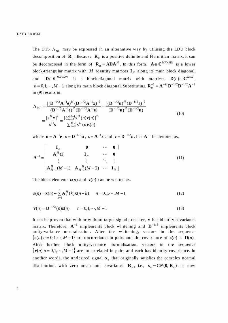
The DTS MFΛ may be expressed in an alternative way by utilising the LDU block

decomposition of uR . Because uR is a positive definite and Hermitian matrix, it can

be decomposed in the form of Hu ADAR = . In this form, MNMN×∈A is a lower

block-triangular matrix with M identity matrices NI along its main block diagonal,

and MNMN×∈D is a block-diagonal matrix with matrices NNn ×∈)(D ,

1,,1,0 −= Mn L along its main block diagonal. Substituting 12/12/11 −−−−− = ADDAR Hu

in (9) results in,

∑∑==

==Λ

−=

−=

−−

−−

−−−−

−−−−

10

10

22

2/12/1

22/12/1

12/112/1

212/112/1

)()(|)()(|||

)()(|)()(|

)()(|)()(|

Mn

H

Mn

HH

H

H

H

H

MF

nnnn

ssνs

ssνs

uDuDεDuD

eADeADxADeAD

H

(10)

where eAu 1−= , uDs 2/1−= , xAε 1−= and εDν 2/1−= . Let 1−A be denoted as,

⎥⎥⎥⎥

⎦

⎤

⎢⎢⎢⎢

⎣

⎡

−−

=

−−

−

NH

MHM

NHN

MM IAA

0IA00I

A

L

MOMM

L

L

)2()1(

)1(

11

11 (11)

The block elements )(nε and )(nν can be written as,

∑ −+==

n

k

Hn knknn

1)()()()( xAxε 1,,1,0 −= Mn L (12)

)()()( 2/1 nnn εDv −= 1,,1,0 −= Mn L (13)

It can be proven that with or without target signal presence, ν has identity covariance matrix. Therefore, 1−A implements block whitening and 2/1−D implements block unity-variance normalisation. After the whitening, vectors in the sequence { }1,,1,0)( −= Mnn Lε are uncorrelated in pairs and the covariance of )(nε is )(nD . After further block unity-variance normalisation, vectors in the sequence { }1,,1,0)( −= Mnn Lν are uncorrelated in pairs and each has identity covariance. In

another words, the undesired signal ux that originally satisfies the complex normal

distribution, with zero mean and covariance uR , i.e., ),(~ uu CN R0x , is now

DSTO-RR-0313

5

transformed into ν that satisfies the complex normal distribution, with zero mean and identity covariance, i.e., ),(~ I0ν CN .

Equation (12) may be viewed as a result of a moving-average (MA) filter in block mode (Roman et al, 2000). The signal )(nx , 1,,1,0 −= Mn L , is estimated by the forward

linear prediction using )( kn −x , nk ,,1L= , with the parameters )(kHnA , nk ,,1L= .

The prediction error is )(nε .

3. Parametric Matched Filter This Section formulates the parametric matched filter (PMF). Roman et al (2000) mention that some simplifications in the MF DTS, MFΛ , lead to the PMF DTS, PMFΛ , to be given below. In fact there is no direct mathematical connections between FMΛ and

PMFΛ , that is, we cannot derive PMFΛ from MFΛ , although we may express both MFΛ and PMFΛ in similar forms.

Assume the data sequence { }1,,1,)( −+= Mppnn Lx is estimated using the thp order

forward autoregressive (AR) parameters )(kHfA , pk ,,1L= . In this process the

forward linear prediction )(ˆ nx for sample )(nx is a linear combination of )( kn −x , pk ,,1L= , as (Marple, Jr, 1987),

∑ −−==

p

k

Hf knkn

1)()()(ˆ xAx 1,,1, −+= Mppn L (14)

The forward linear prediction residual is,

∑ −=−==

p

k

Hf knknnn

0)()()(ˆ)()( xAxxε 1,,1, −+= Mppn L (15)

where NHf IA =)0( . The count n of )(nε in (15) starts from p , which is not

convenient. By shifting the count n of )(nε to start from zero, (15) can be rewritten as,

∑ +−==

p

k

Hf pknkn

0)()()( xAε 1,,1,0 −−= pMn L (16)

Although (16) and (12) use similar symbols, this is adopted to avoid using too many symbols. Note that the subscript f of )(kH

fA in (16) simply means the forward

DSTO-RR-0313

6

prediction. Unlike in (12), )(kHfA is now independent of n . Also )(kH

fA in (16) in

general has nothing mathematically to do with )(kHnA in (12). This will become clear

after the derivation of )(kHfA is given in the following subsection.

Similarly we may define the steering residual 1)( ×−∈ NpMu as,

∑ +−==

p

k

Hf pknkn

0)()()( eAu 1,,1,0 −−= pMn L (17)

It is worth noting that the dimensionality of the thp order ε and u is reduced to 1)( ×− NpM .

Equations (16) and (17) can be written in more compact forms as,

Bx

ε

εε

ε =

⎥⎥⎥⎥

⎦

⎤

⎢⎢⎢⎢

⎣

⎡

−−

=

)1(

)1()0(

pMM

(18)

Be

u

uu

u =

⎥⎥⎥⎥

⎦

⎤

⎢⎢⎢⎢

⎣

⎡

−−

=

)1(

)1()0(

pMM

(19)

where the block matrix MNNpM ×−∈ )(B has the form of

⎥⎥⎥⎥⎥

⎦

⎤

⎢⎢⎢⎢⎢

⎣

⎡

−

−−

=

NHf

Hf

NHf

Hf

NHf

Hf

pp

pppp

IAA00

00IAA000IAA

B

LL

O

LL

LL

)1()(

)1()()1()(

(20)

Let )}()({)( nnEn HεεR =ε denote the temporal residual covariance matrix which is Hermitian and positive definite. The LDU decomposition of )(nεR is,

)()()()( nnnn Hεεεε LDLR = (21)

DSTO-RR-0313

7

where NNn ×∈)(εL is a lower triangular matrix and its main diagonal elements are

unity and NNn ×∈)(εD is a diagonal matrix with its all diagonal elements greater than zero. The transfer matrix )(nT functioning as both the whitening and unity-variance normalisation for )(nε is then,

)()()( 12/1 nnn −−= εε LDT (22)

Finally the PMF DTS can be defined as,

∑∑==Λ

−−=

−−=

10

10

22

)()(|)()(|||

pMn

H

pMn

HH

PMF nnnn

ssνs

ssνs

H (23)

where )()()( nnn uTs = and )()()( nnn εTν = . Equation (23) can be expressed in a compact form with the use of input signal x and steering vector e as,

eCexCe

ssνs

Hp

Hp

HH

PMF

22 ||||==Λ (24)

where

BRBC 1−= εH

P (25)

⎥⎥⎥⎥

⎦

⎤

⎢⎢⎢⎢

⎣

⎡

−−

=

)1(

)1()0(

pMε

ε

ε

ε

R

RR

RO

(26)

Therefore, analogous to STAP, we may define the PMF weighting vector 1×∈ MN

PMF w as,

eCw PPAMF γ= (27)

The corresponding SINR and adaptive pattern, respectively, are,

eCeeCRCe

eCewRw

ew

uP

Ht

PPH

PH

t

PMFuHPMF

HPMFt

PMFSINR ξξξ

===22 ||||

(28)

and

DSTO-RR-0313

8

2|),(| tdtsHPMFPMF ffP ew= (29)

Comparing (24) and (9) or (28) and (7), we see that the matrix PC in (24) and (28)

functions as the matrix 1−uR in (9) and (7).

3.1 Determination of Parameters in Parametric Matched Filtering In the previous subsection we have derived for the PMF algorithm all formulae except the filter parameters )(kH

fA , pk ,,1L= . Different methodologies lead to different algorithms for finding the parameters (Marple, Jr, 1987). Here we follow the least squares method, i.e., the covariance method (Marple, Jr, 1987). Roman et al (2000) has reported that in the context of radar signal processing, the least squares method usually outperforms other methods, such as the Strand-Nuttall method. The derivation below is independent work of the author.

The goal of the least squares method is to find parameters )(kHfA , pk ,,1L= , which

produce a minimum squared residual, εεH . To find the minimum squared residual,

we need to solve the simultaneous equations 0)(

=∂

∂ εεA

HHf k

, pk ,,1 L= (note that

NHf IA =)0( is constant). The derivative of a scalar function 11)( ×∈Qf with respect

to nm×∈Q is an nm× matrix (Van Trees, 2002, p. 1399),

⎥⎥⎥

⎦

⎤

⎢⎢⎢

⎣

⎡

∂∂∂∂

∂∂∂∂=

∂∂

mnm

n

qfqf

qfqff

//

//)(

1

111

O

L

QQ

(30)

where ikq , mi ,,1L= , nk ,,1L= , is the element of Q . After tedious but

straightforward algebra, the equation satisfying 0)(

=∂

∂ εεA

HHf k

, pk ,,1L= , is,

[ ] NpN

N

f

f

fff

p

×∈=

⎥⎥⎥⎥

⎦

⎤

⎢⎢⎢⎢

⎣

⎡

0

IA

A

RR)1(

)(

1M

(31)

Therefore we find the parameters as,

DSTO-RR-0313

9

⎥⎥⎥

⎦

⎤

⎢⎢⎢

⎣

⎡−=

⎥⎥⎥⎥⎥⎥

⎦

⎤

⎢⎢⎢⎢⎢⎢

⎣

⎡

=

−

N

fff

f

f

f

f

p

I

RR

A

A

A

A1

1

)0(

)1(

)(M

(32)

where pNpNff

×∈R and NpNf

×∈1R are sub-block matrices of NpNpf

)1()1( +×+∈R given by,

}{1110

1 Hff

fff

f E XXRR

RRR =

⎥⎥⎦

⎤

⎢⎢⎣

⎡= (33)

⎥⎥⎥⎥

⎦

⎤

⎢⎢⎢⎢

⎣

⎡

−+

−−−

=

)1()1()(

)()2()1()1()1()0(

Mpp

pMpM

f

xxx

xxxxxx

X

L

O

L

L

(34)

If the covariance matrix uR is known, fR can be formed by summing up pM −

block matrices of uR using a moving NpNp )1()1( +×+ window diagonally from top to bottom, which may be expressed as,

∑ +=−−

=

1

0):(

pM

kuf pkkRR (35)

where NpNpu pkk )1()1():( +×+∈+ R is a block sub-matrix of uR , with

NNu kk ×∈),(R as its top left block element and NN

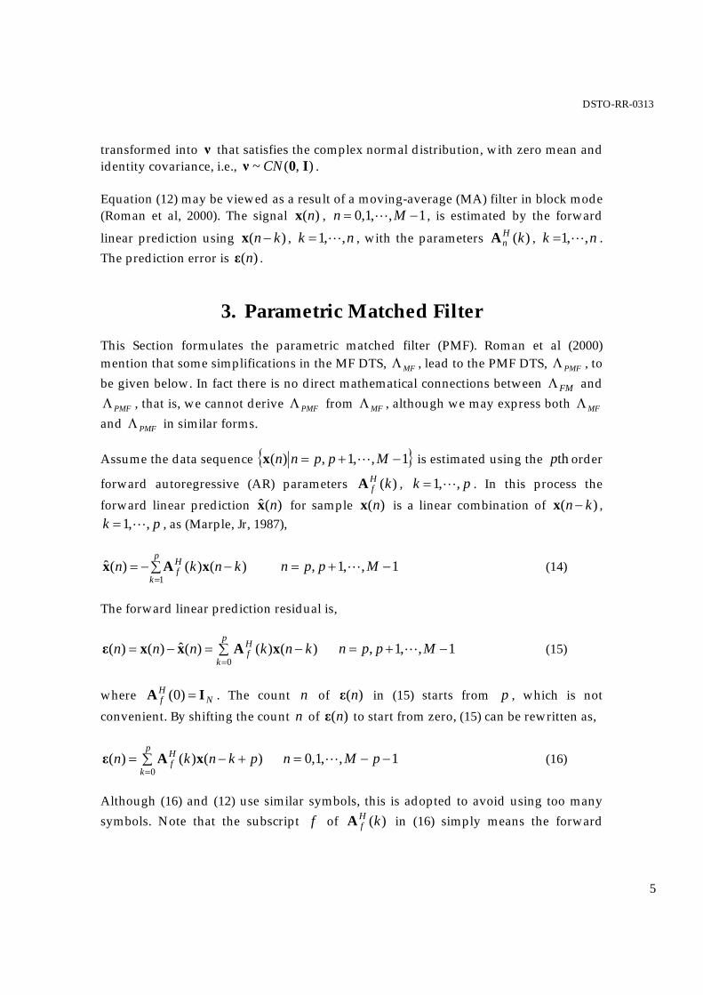
u pkpk ×∈++ ),(R as its bottom right block element. Figure 1 depicts a situation where fR is formed by adding four

sub-block matrices of uR , corresponding to the case of 2=p and 6=M . It can be seen that the PMF algorithm does not use all block elements in uR to form fR . This may

be considered as an information loss since the block element ),( kiuR stands for the correlation between data collected by the thi and thk pulses and its neglect means that the correlation is treated as zero.

DSTO-RR-0313

10

Ru(0,0) Ru(0,1) Ru(0,2) Ru(0,3) Ru(0,4) Ru(0,5)

Ru(5,0) Ru(5,1) Ru(5,2) Ru(5,3) Ru(5,4) Ru(5,5)

Ru(1,0) Ru(1,1) Ru(1,2) Ru(1,3) Ru(1,4) Ru(1,5)

Ru(4,0) Ru(4,1) Ru(4,2) Ru(4,3) Ru(4,4) Ru(4,5)

Ru(2,0) Ru(2,1) Ru(2,2) Ru(2,3) Ru(2,4) Ru(2,5)

Ru(3,0) Ru(3,1) Ru(3,2) Ru(3,3) Ru(3,4) Ru(3,5)

Figure 1: fR is formed by summing up sub-block matrices of uR using a moving window for

the case of 2=p and 6=M . Some of the block elements of uR are not used in forming fR .

4. Parametric Adaptive Matched Filter (PAMF) In general the covariance matrix of undesired signals uR is unknown, so it has to be estimated adaptively using range samples. The often used method is the diagonally-loaded sample matrix (DL-SM) method (Carlson, 1988, Ward and Kogon, 2004), as,

IxxR δ+∑==

K

k

Hkku K 1

1ˆ (36)

where the subscript k denotes range bins. δ is a small value of the order of the system thermal noise level.

The transfer matrix )(nT 1,,1,0 −−= pMn L given by (22) is time-dependent. Roman et al (2000) suggest that a single time-independent transfer matrix T may replace the time-dependent transfer matrix )(nT in the adaptive process. The time-independent transfer matrix T is obtained through a time-averaging process as,

ffHf

pM

nf pM

npM

ARARR−

=∑−

=−−

=

1)(1 1

0εε (37)

Hf εεεε LDLR = (38)

DSTO-RR-0313

11

12/1 −−= εε LDT (39)

The PAMF DTS is defined as,

∑∑==Λ

−−=

−−=

10

10

22

)()(|)()(|||

pMn

H

pMn

HH

PAMF nnnn

ssνs

ssνs

H (40)

Expressions (40) and (23) are the same, but the difference between PMFΛ and PAMFΛ is

that uR and )(nT 1,,1,0 −−= pMn L , are used for PMF whereas uR̂ and T are used for PAMF.

Equation (40) can be written in a more compact matrix notation with input signal x and steering vector e (Michels et al, 2003). In order to do so, we write,

⎥⎥⎥⎥

⎦

⎤

⎢⎢⎢⎢

⎣

⎡

−−⎥⎥⎥⎥

⎦

⎤

⎢⎢⎢⎢

⎣

⎡

=

⎥⎥⎥⎥

⎦

⎤

⎢⎢⎢⎢

⎣

⎡

−− )1(

)1()0(

)1(

)1()0(

pMpM ε

εε

T

TT

ν

νν

MOM (41)

This equation can be written as,

BxTIεTIν )()( ⊗=⊗= −− pMpM (42)

Similarly,

BeTIuTIs )()( ⊗=⊗= −− pMpM (43)

Therefore,

xCeνs HPA

H = (44)

eCess HPA

H = (45)

where

BRIB

BTTIB

BTITIBC

)(

)(

))((

1−−

−

−−

⊗=

⊗=

⊗⊗=

εfpMH

HpM

H

pMH

pMH

PA

(46)

DSTO-RR-0313

12

Inserting (44) and (45) in (40), we can express the PAMF DTS as,

eCexCe

PAH

PAH

PAMF

2||=Λ (47)

Similarly the matrix PAC in (47) functions as 1−uR in (9). The PAMF weighting vector

MNPAMF ∈w defined implicitly in (47) is,

eCw PAPAMF γ= (48)

The SINR for the PAMF is,

eCRCeeCe

u PAPAH

PAH

tPAMFSINR ˆ

|| 2ξ= (49)

The adaptive pattern of the PAMF is,

2|),(| tdtsHPAMFPAMF ffP ew= (50)

From the above derivation, we may observe some features of the PAMF approach:

• The estimation of the PAMF parameters (coefficients) is achieved by averaging measures not only from a series of range cells collected by the same pulse (Equation (36), fast-time) but also from a series of pulses (Equation (37), slow-time). Hence the estimation procedure is enhanced through the use of both fast-time and slow-time data averaging process.

• It can be seen from Figure 1 that the PAMF does not use the full covariance matrix. In another words, some correlations between data collected by different pulses are treated as zero. This approximation may degrade the performance if the actual correlations are high.

• The original data snapshot consists of a time sequence of M points. Both the PMF and PAMF processes are dimensionality-reduced transformations and contain only a time sequence of pM − points. As we know that the Doppler resolution as well as coherent processing gain is dependent on the length of the time sequence, the reduction in time sequence decreases the Doppler resolution as well as the processing gain. This may not be a concern if pM >> . However in the case where the ratio MpM /)( − is low, the loss in the coherent processing gain and the loss in the Doppler resolution may become significant. Section 7 proposes a modified version of PAMF, which does not induce any dimensionality loss.

DSTO-RR-0313

13

5. Performance Results

5.1 Generic Radar Model Data A simple radar model (Ward, 1994) was first used to assess the performance of PMF. Table 1 lists the parameters of the model. The clutter model, which is often referred to as the first-order clutter model, does not take account of temporal and spatial correlation effects (Klemm, 2002) and has the following features,

• Constant clutter coefficient; • Uncorrelated clutter echoes from patch to patch; • No range fold-over effect; • No clutter intrinsic motion.

Table 1: Parameters used in the generic radar model.

Parameter Specification Radar

Phased array Linear 18-by-4 elements, element pattern ( )φcos , half-wavelength element spacing,

uniform tapering PRF 300Hz Number of pulses per CPI 18 Looking direction Broadside, horizontal

Platform Height 9km Speed 1)/(2 =dfv prfa (DPCA condition), where d

is the element spacing Undesired signals

Thermal noise Gaussian Clutter First-order clutter model, CNR = 47dB Jamming Two equal-intensity broadband jamming

signals at azimuth angles of 65o and 130o, respectively, JNR = 38dB

Under these assumptions, the covariance matrix uR can be formed (Ward, 1994, Dong,

2005). Since uR is strictly a Toeplitz-bock-Toeplitz matrix, )(nTT = , 1,,1,0 −−= pMn L . Therefore, there is no discrimination between PMF and PAMF,

and the results of PMF and PAMF are the same. Figure 2 (a) shows the SINR comparison between the MF and PMF ( 3=p ) processes. The SINR loss of PMF due to

DSTO-RR-0313

14

dimensionality loss compared to the MF SINR is shown in Figure 2 (b). The SINR loss due to the dimensionality loss in theory is 79.0)18/15(log10 10 −= dB.

-30

-20

-10

0

10

20

30

-150 -100 -50 0 50 100 150

Doppler frequency (Hz)

SIN

R (d

B)

SINR_MF

SINR_PMF

Figure 2 (a): SINR comparison between MF and PMF ( 3=p ). There is a little PMF SINR loss compared to the MF SINR.

-4

-3

-2

-1

0

-150 -100 -50 0 50 100 150

Doppler frequency (Hz)

SIN

R d

iffer

ence

(dB)

PMF / MF

Figure 2 (b): The SINR loss of PMF due to the dimensionality loss.

Assume a target signal tx which has a constant amplitude (SNR = 0dB) and constant Doppler (100Hz) is embedded in undesired signals including clutter ),,(~ cc CN R0x jamming ),,(~ jj CN R0x and thermal noise ),(~ nn CN R0x , that is,

njct xxxxx +++= and njcu RRRR ++= . Figure 3 shows the snapshots of clutter,

jamming, thermal noise and target signals. The resultant PMFΛ is compared with

DSTO-RR-0313

15

MFΛ in Figure 4. It can be seen from the PAM result that there is a small loss in the peak, and a slight broadening of the mainlobe due to the dimensionality reduction problem as discussed earlier.

-60

-45

-30

-15

0

15

0 54 108 162 216 270 324

space-time sequence

Sign

al le

vel (

dB)

x_c

x_j

x_n

x_t

Figure 3: Snapshots of clutter, jamming, noise and target signals.

-20

-10

0

10

20

30

-150 -100 -50 0 50 100 150Doppler frequency (Hz)

Sig

nal l

evel

(dB

) MF

PMF

Figure 4: Performance comparison between PMFΛ and MFΛ .

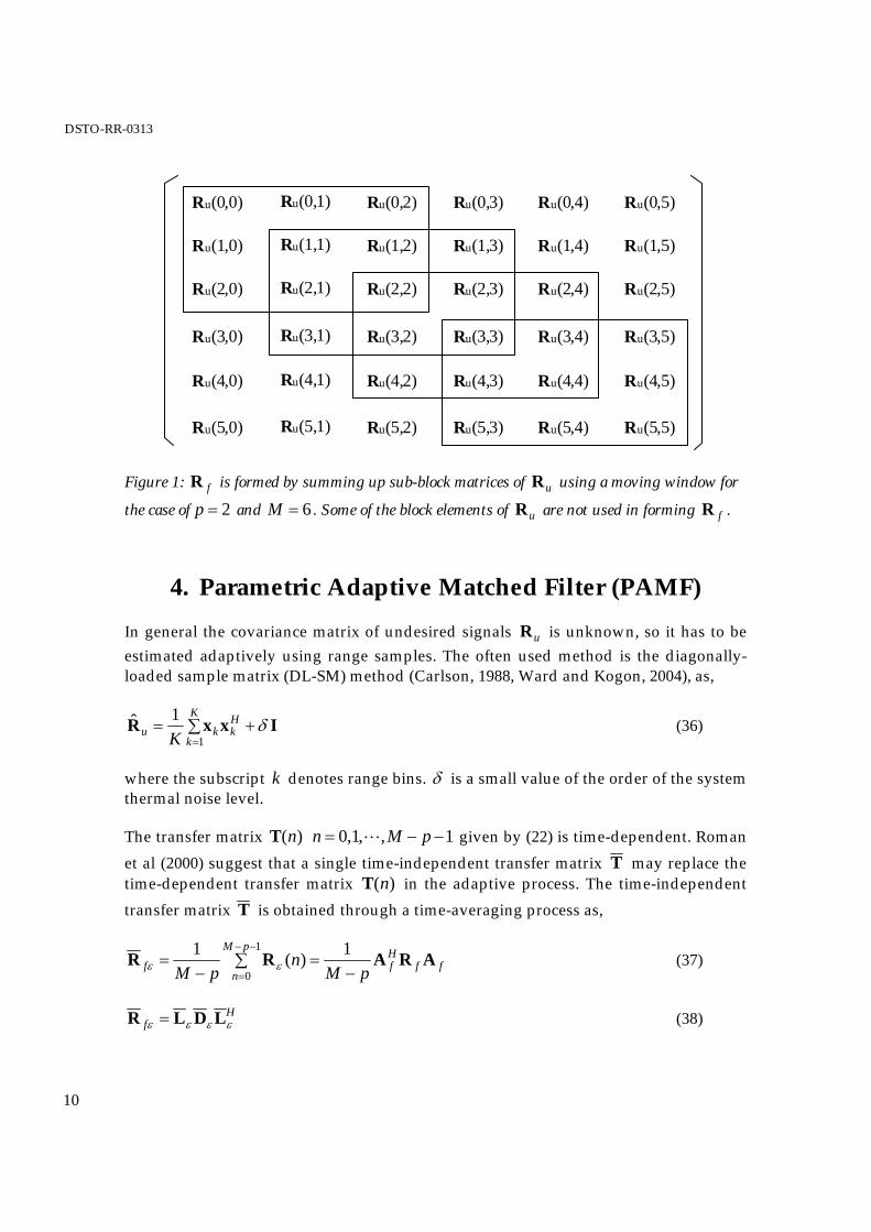
Finally the MF and PMF adaptive patterns are shown in Figure 5 assuming a target signal to be at zero azimuth with 100Hz Doppler. The two patterns are very similar.

It can be concluded from the above analysis, for this simulation, that MF and PMF perform approximately the same for this simple radar model.

DSTO-RR-0313

16

(a) MF

(b) PMF, 3=p

Figure 5: MF and PMF adaptive patterns.

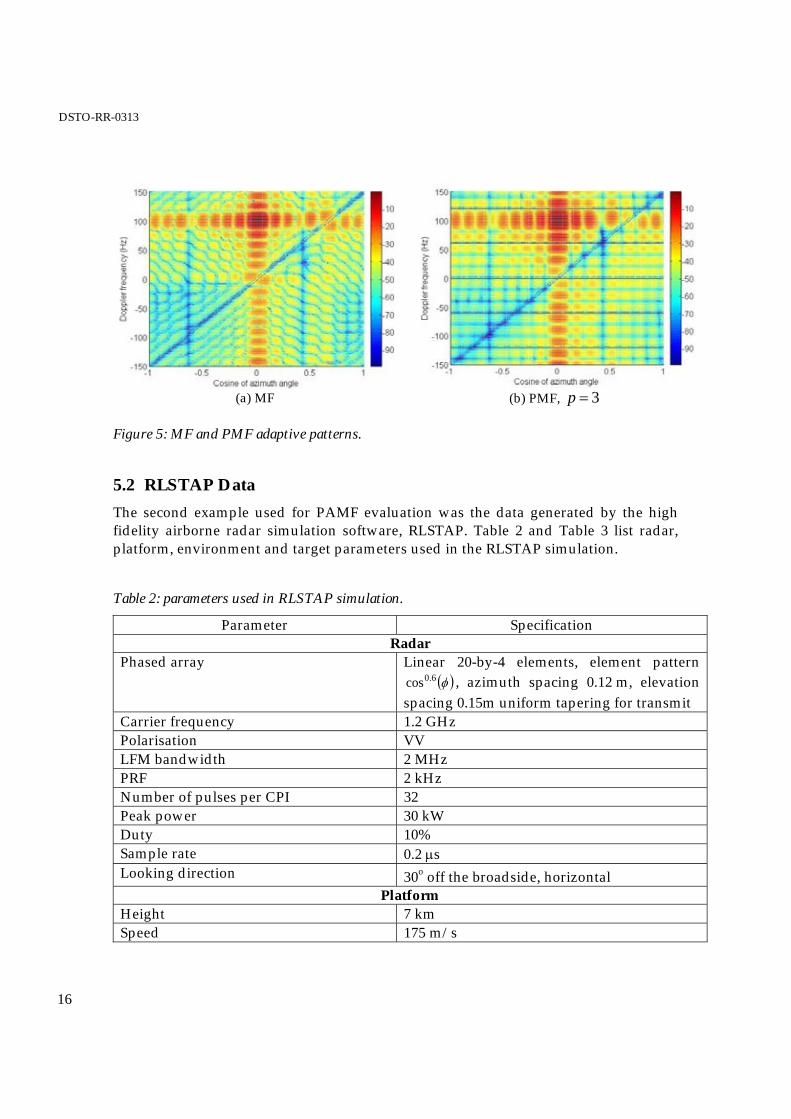
5.2 RLSTAP Data The second example used for PAMF evaluation was the data generated by the high fidelity airborne radar simulation software, RLSTAP. Table 2 and Table 3 list radar, platform, environment and target parameters used in the RLSTAP simulation.

Table 2: parameters used in RLSTAP simulation.

Parameter Specification Radar

Phased array Linear 20-by-4 elements, element pattern ( )φ6.0cos , azimuth spacing 0.12 m, elevation

spacing 0.15m uniform tapering for transmit Carrier frequency 1.2 GHz Polarisation VV LFM bandwidth 2 MHz PRF 2 kHz Number of pulses per CPI 32 Peak power 30 kW Duty 10% Sample rate 0.2 μs Looking direction 30o off the broadside, horizontal

Platform Height 7 km Speed 175 m/s

DSTO-RR-0313

17

Undesired signals Thermal noise Gaussian Clutter Washington D.C. area Jamming None

Table 3: Target parameters used in the RLSTAP simulation.

Parameters Target 1 Target 2 Target 3 Height (km) 3 3 3 Position off mainlobe direction 1 km north 0.5 km south 0 Radial velocity (m/s) -100 -20 150 Doppler frequency (Hz) -500 860 -500 Range (km) 50 60 70 RCS (sqm) 1 1 1

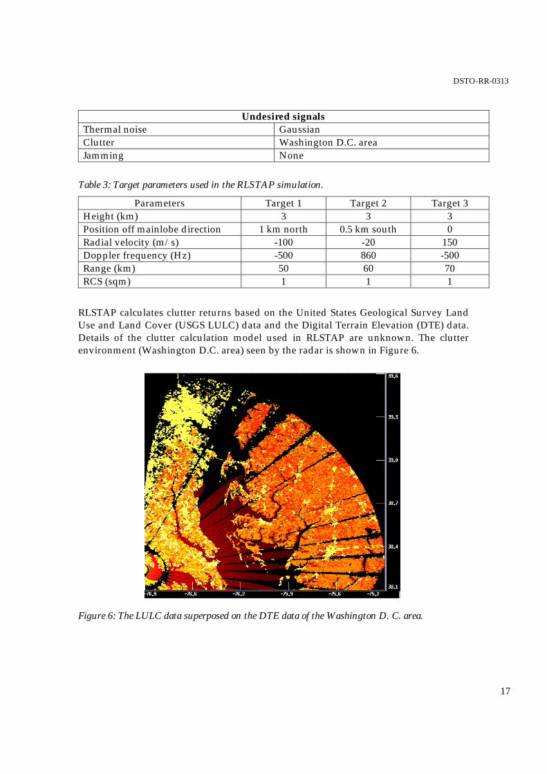
RLSTAP calculates clutter returns based on the United States Geological Survey Land Use and Land Cover (USGS LULC) data and the Digital Terrain Elevation (DTE) data. Details of the clutter calculation model used in RLSTAP are unknown. The clutter environment (Washington D.C. area) seen by the radar is shown in Figure 6.

Figure 6: The LULC data superposed on the DTE data of the Washington D. C. area.

DSTO-RR-0313

18

The unambiguous range is 75km for the parameters given in Table 2. With the classical 4/3 Earth radius model, the range to the horizon is 345km resulting in up to four range foldovers. However due to the availability of the LCLU data, the simulation only took the first range foldover into the account. That is, clutter returns from beyond 150km were ignored. Because the clutter return decays as a function of the range to the third power, the effect of higher range foldovers is believed to be insignificant. Accordingly, data collected by the first pulse are discarded in the process, as they do not contain the clutter returns from ambiguous ranges. Therefore the actual number of pulses used in the process was 31=M .

To obtain the covariance matrix using the DL-SM method, one might think that the more range samples the better. In fact this is not necessarily true because samples are generally not collected from a statistically homogenous clutter environment. We used four different sampling methods and visually compared the performance of MF for target detection. The ranges bins used in these four cases are,

• Case 1: range bins 800-2650 with the exclusion of target range bins themselves (the target range bins for targets 1, 2 and 3 are 1934, 2266 and 2598, respectively) as well as the 10 nearest range bins on both sides of each target range bin;

• Case 2: range bins 1634-2234 with the exclusion of 1924-1944 (the target range bin is 1934)

• Case 3: range bins 801-1600 (no target in this region); • Case 4: range bins 1001-1600 (no target in this region).

It has been found that case 1 performed the worst, although it used the most range bins. Cases 3 and 4 performed approximately the same and better than the first two cases. Case 4 was used in the following performance comparison between MF and PAMF.

The SINR comparison between MF and PAMF ( 3=p ) is shown in Figure 7 (a). It is seen that the PAMF SINR shows some noticeable but not significant loss in the clutter notch region in comparison with the MF SINR apart from the loss caused by the dimensionality loss. The SINR loss due to the dimensionality loss in theory is

44.0)31/28(log10 10 −= dB.

DSTO-RR-0313

19

-20

-10

0

10

20

30

40

-1000 -500 0 500 1000Doppler frequency (Hz)

SIN

R (d

B)

MF (STAP)

PAMF

Figure 7 (a): SINR comparison between MF and PAMF. The PAMF SINR, compared to the MF SINR, shows some not significant but noticeable loss in the vicinities of the clutter notch.

-3

-2.5

-2

-1.5

-1

-0.5

0

-1000 -500 0 500 1000

Doppler frequency (Hz)

SIN

R d

iffer

ence

(dB)

PAMF / MF

Figure 7 (b): The SINR loss of PAMF due to the dimensionality loss.

Results of MF DTS and PAMF DTS are shown in Figure 8. The performances of the two processors seem approximately the same at first glance. Careful observation, however, indicates that the signal level of target 2 (the target in the middle range bin) in the PAMF process is a few dB lower than the level in the MF process, which is due to the PAMF SINR loss for that frequency as shown in Figure 7. Figure 9 and Figure 10 replot Figure 8 into 2D plots, i.e., signal level versus range and Doppler frequency, respectively. There are only two targets shown in Figure 10, because target 1 (near range) and target 3 (far range) have the same Doppler (refer to Table 3) and are superposed. Figure 9 (a) shows the presence of spikes which could increase the false alarm rate or reduce the detection probability. We will see in due course that these spikes in fact exist in the results of both MF and PAMF DTS processes (though the spikes are much reduced for the PAMF process for this example as shown in Figure 9

DSTO-RR-0313

20

(b)) and could become much worse for MCARM data. We discuss what causes these spikes and how to mitigate them in the next subsection.

(a) MF

(b) PAMF, 3=p

Figure 8: Target detection performance comparison between MF DTS and PAMF DTS.

(a) MF

(b) PAMF, 3=p

Figure 9: Target detection performance comparison between MF DTS and PAMF DTS, plotted as signal level verses range bin.

DSTO-RR-0313

21

(a) MF

(b) PAMF, 3=p

Figure 10: Target detection performance comparison between MF DTS and PAMF DTS, plotted as signal level verses Doppler frequency.

If we increase the order of the parameter filter, p , say, from 3 to 5, the SINR loss in the vicinity of the clutter notch for the PAMF is reduced but at the cost of Doppler resolution reduction1. Figure 11 shows the detection result of PAMF with 5=p where we can see the signal level of target 2 having been improved compared to the result of

3=p shown in Figure 9 (b).

(a) Signal level versus range

(b) Signal level versus Doppler

Figure 11: Using a higher order parameter filter, 5=p , improves the level of target 2 (the middle range target), but at the cost of Doppler resolution reduction in the PAMF processing.

1 It means poorer Doppler resolution.

DSTO-RR-0313

22

5.2.1 Discussions on Detection Test Statistics

Detection test statistics, MFΛ , PMFΛ and PAMFΛ for MF, PMF, and PAMF, respectively, have been given in (9), (24), and (47), previously. However we have found these test statistics are sensitive to Doppler frequencies of the mainlobe clutter, which may impose a difficulty with target detection and increase the false alarm rate. To explain, let us examine MFΛ from another perspective. When 1=tξ , (7) can be written as,

eRewRwew 1

2||)1( −=== uH

MFuHMF

HMF

tMFSINR ξ (51)

Using the result of (51) we express MFΛ on the decibel scale as,

)1(log10||log10log10 102

1010 =−=Λ tMFHMFMF SINR ξxw (52)

Equation (52) indicates that on the decibel scale MFΛ is the output of the signal minus the SINR of the processor. In general, the SINR of the processor is a constant everywhere except in the frequency vicinity of the mainlobe clutter, where a deep notch is placed (for instance, see Figure 7). Therefore MFΛ on the decibel scale is the output of the processor plus a frequency-independent constant (small in value) outside of the notch region, or a frequency-dependent variable (large in value) in the notch region. The slope of the notch is steep and varies rapidly with frequency. On the other hand, individual data snapshot x is a random process whose frequency components in the notch region (i.e. clutter) may vary significantly. Therefore, we can expect that fluctuations of MFΛ in the notch region could occur from range bin to range bin, and impose a difficulty on the use of MFΛ for target detection. In fact our interests in target detection using the MF process are generally outside of the clutter notch region. Therefore, simply using the output of the processor, 2

10 ||log10 xwHMF , as a detection

test statistic may provide a better result. In order to discriminate, we refer to this as the modified detection test statistic (MDTS). Similar discussion can be made for the other two detection test statistics, PMFΛ and PAMFΛ .

The detection results shown in Figure 12 and Figure 13 are obtained with the use of MDTS. It can be seen that the spikes disappear while a notch at the clutter Doppler frequency appears.

DSTO-RR-0313

23

(a) MF MDTS, signal level versus range

(b) MF MDTS, signal level versus Doppler

Figure 12: MDTS removes spikes in the vicinity of mainlobe clutter Doppler frequency, but leaves a notch at that frequency.

(a) PAMF MDTS, 5=p , signal level versus

range

(b) PAMF MDTS, 5=p , signal level versus

Doppler

Figure 13: MDTS removes spikes in the vicinity of mainlobe clutter Doppler frequency, but leaves a notch at that frequency.

5.2.2 Minimum Number of Range Samples The unknown covariance matrix of undesired signals is usually estimated using range samples as shown in (33). The conventional question asked is how many range samples are required in order to obtain a reliable estimate of the matrix? Detailed discussions are available in the literature and are out of the scope of this report. Here we only intend to have some discussions from the viewpoint of practical application.

DSTO-RR-0313

24

It is well known that given a 3dB tolerance of the optimum performance the number of identically independently distributed (iid) samples needed for estimating a covariance matrix is twice the dimension of the matrix (Reed et al, 1974). However, for the equidistant antenna array and constant PRF, the structure of the covariance matrix has a Toeplitz-block-Toeplitz structure, and the required minimum number of range samples can be greatly reduced (Steiner and Gerlach, 1998, Steiner and Gerlach, 2000, Gerlach and Picciolo, 2003, Bresler, 1998).

In general if we know the eigenvalue distribution of the covariance matrix, we can estimate the minimum number of iid samples required for the covariance matrix. The rank of the covariance matrix of clutter is given by Brennan’s rule as (Brennan and Staudaher, 1992, Ward, 1994),

)}1(int{ −+= MNNr β (53)

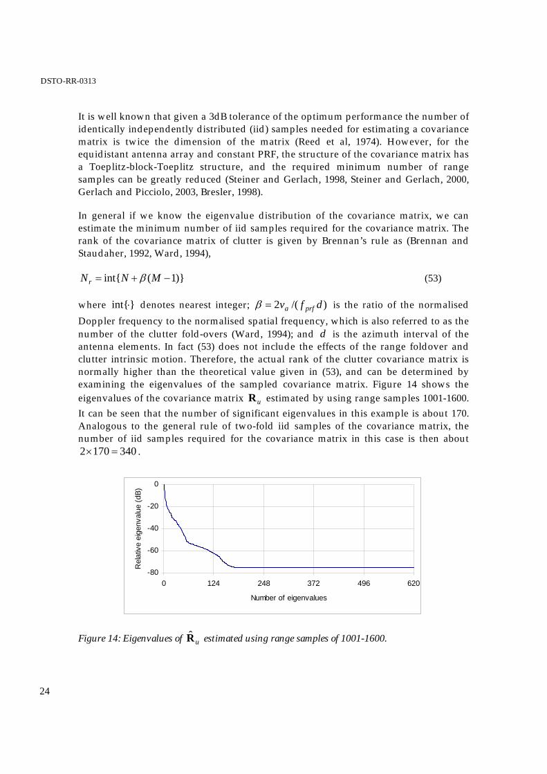
where }int{⋅ denotes nearest integer; )/(2 dfv prfa=β is the ratio of the normalised Doppler frequency to the normalised spatial frequency, which is also referred to as the number of the clutter fold-overs (Ward, 1994); and d is the azimuth interval of the antenna elements. In fact (53) does not include the effects of the range foldover and clutter intrinsic motion. Therefore, the actual rank of the clutter covariance matrix is normally higher than the theoretical value given in (53), and can be determined by examining the eigenvalues of the sampled covariance matrix. Figure 14 shows the eigenvalues of the covariance matrix uR estimated by using range samples 1001-1600. It can be seen that the number of significant eigenvalues in this example is about 170. Analogous to the general rule of two-fold iid samples of the covariance matrix, the number of iid samples required for the covariance matrix in this case is then about

3401702 =× .

-80

-60

-40

-20

0

0 124 248 372 496 620

Number of eigenvalues

Rel

ativ

e ei

genv

alue

(dB)

Figure 14: Eigenvalues of uR̂ estimated using range samples of 1001-1600.

DSTO-RR-0313

25

One significant feature of the PAMF, according to Roman et al (2000) is that the method still performs even using a relatively small number of range samples to adaptively estimate parameters. This is because the parameters )(kH

fA ,

1,,1,0 −−= pMk L , are estimated using fR̂ rather than uR̂ . The dimension of fR is

usually much smaller than that of uR , and so is the number of the dominant eigenvalues. Therefore the number of range samples required for estimating parameters of PAMF can be significantly fewer than the number of samples for estimating the covariance matrix in the conventional MF method. Figure 15 shows the eigenvalue distributions of fR with 3=p and 5=p estimated using range samples 1001-1600. We make two observations from the figure. First, the number of dominant eigenvalues are about the same (26 for 3=p and 28 for 5=p ) although the dimension

of NpNpf

)1()1( +×+∈R varies with p , thus suggesting that using a higher order of p in the PAMF process does not require more iid samples. Second, the number of dominant eigenvalues in fR is significantly smaller than that of uR , so the PAMF method requires far fewer samples in general.

-80

-60

-40

-20

0

0 20 40 60 80 100 120

Number of eigenvalues

Rel

ativ

e ei

genv

alue

(dB)

p = 3

p = 5

Figure 15: Eigenvalues of fR̂ , 3=p and 5=p , estimated using range samples of 1001-1600.

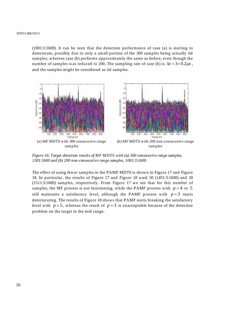
We notice that the range resolution of the system shown in Table 2 is )2/( Bcr =Δ where c is speed of light and B the bandwidth of the LMF. The corresponding range sampling rate should be sBt μ5.0/1 ==Δ . The actual range sampling rate used in RLSTAP was an over-sampled rate of sμ2.0 . Therefore, the consecutive range samples may not be iid samples. Shown in Figure 16 are the MF MDTS results with the covariance matrix obtained by averaging (a) 300 consecutive range samples (1301:1600), and (b) 200 non-consecutive range samples with a interval of 3

DSTO-RR-0313

26

(1001:3:1600). It can be seen that the detection performance of case (a) is starting to deteriorate, possibly due to only a small portion of the 300 samples being actually iid samples, whereas case (b) performs approximately the same as before, even though the number of samples was reduced to 200. The sampling rate of case (b) is st μ2.03×=Δ , and the samples might be considered as iid samples.

(a) MF MDTS with 300 consecutive range

samples

(b) MF MDTS with 200 non-consecutive range

samples

Figure 16: Target detection results of MF MDTS with (a) 300 consecutive range samples, 1301:1600 and (b) 200 non-consecutive range samples, 1001:3:1600.

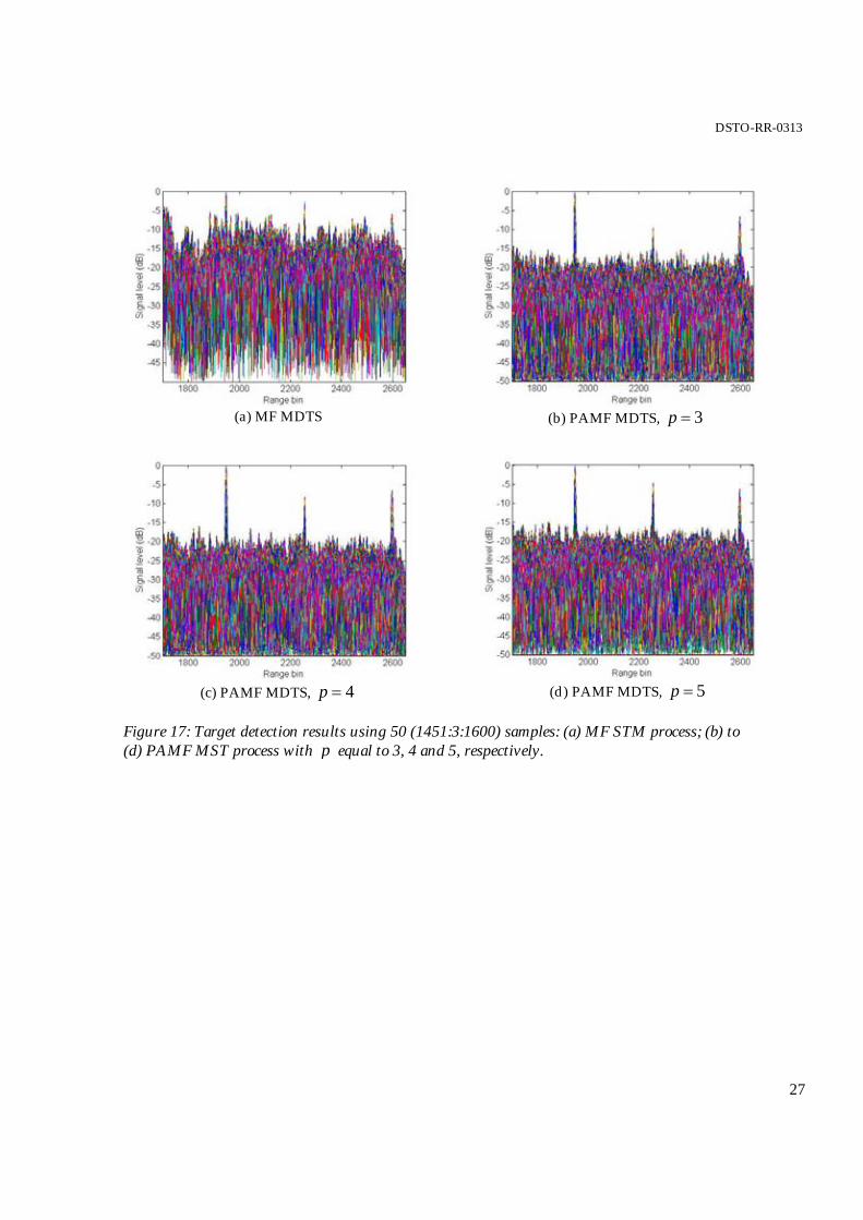
The effect of using fewer samples in the PAMF MDTS is shown in Figure 17 and Figure 18. In particular, the results of Figure 17 and Figure 18 used 50 (1451:3:1600) and 30 (1511:3:1600) samples, respectively. From Figure 17 we see that for this number of samples, the MF process is not functioning, while the PAMF process with 4=p or 5 still maintains a satisfactory level, although the PAMF process with 3=p starts deteriorating. The results of Figure 18 shows that PAMF starts breaking the satisfactory level with 5=p , whereas the result of 3=p is unacceptable because of the detection problem on the target in the mid range.

DSTO-RR-0313

27

(a) MF MDTS

(b) PAMF MDTS, 3=p

(c) PAMF MDTS, 4=p

(d) PAMF MDTS, 5=p

Figure 17: Target detection results using 50 (1451:3:1600) samples: (a) MF STM process; (b) to (d) PAMF MST process with p equal to 3, 4 and 5, respectively.

DSTO-RR-0313

28

PAMF MDTS, 3=p

PAMF MDTS, 5=p

Figure 18: Target detection using the PAMF MDTS process with 30 non-consecutive samples, 1511:3:160): (a) 3=p and (b) 5=p .

5.2.3 Selection of Secondary Data

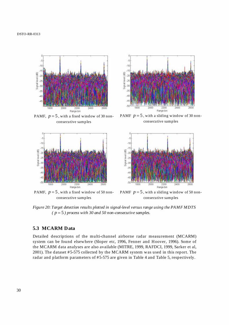
Data used for sampling uR or fR are sometimes referred to as secondary data in contrast to primary data which are under test using the statistics of the secondary data. The primary data and secondary data are mutually exclusive. Generally one may use a sliding window or a fixed window to select secondary data (Ward and Kogon, 2004). With the sliding window architecture, the CUT as well as a few guard cells, which normally sit in the centre of the window, are excluded from the sliding window. Since each CUT corresponds to a unique sliding window, it is computationally very expensive. With the fixed window architecture, a single uR̂ or fR̂ estimated from a fixed window is used and applied to a block of cells rather than a single cell. All the previous results of RLSTAP data were generated using a fixed window as specified. Theoretically, the sliding window seems to be able to provide better results but has a huge computational cost. However this is not observed in simulation. Figure 19 and Figure 20 compare the PAMF MDST results using a fixed window against a sliding window. The fixed window used was 30 or 50 non-consecutive samples with an interval of 3 (1511:3:1600 or 1451:3:1600). The sliding window also used 30 or 50 non-consecutive samples at an interval of 3, symmetrically on the sides of the CUT plus 5 guard cells at each side. That is, for a CUT k , the sliding window consists of

)6:3:3156( −×−− kk and )3156:3:6( ×+++ kk or )6:3:3256( −×−− kk and )3256:3:6( ×+++ kk . We see that little is gained using the sliding window against

the fixed window. This is in fact consistent with the findings reported previously (Dong, 2005). The report (Dong, 2005) shows that first the inverse of the covariance matrix is approximately invariant to changes in clutter range cells, and second, the weighting vector is not sensitive to the changes of grazing angle in a certain region.

DSTO-RR-0313

29

These two findings explain that a single weighting vector can be applied to a segment of range cells.

PAMF, 5=p , with a fixed window of 30 non-

consecutive samples

PAMF 5=p , with a sliding window of 30

non-consecutive samples

PAMF, 5=p , with a fixed window of 50 non-

consecutive samples

PAMF 5=p , with a sliding window of 50

non-consecutive samples

Figure 19: Target detection results plotted in signal-level versus range and Doppler using the PAMF ( 5=p ) MDTS process with 30 and 50 non-consecutive samples.

DSTO-RR-0313

30

PAMF, 5=p , with a fixed window of 30 non-

consecutive samples

PAMF 5=p , with a sliding window of 30 non-

consecutive samples

PAMF, 5=p , with a fixed window of 50 non-

consecutive samples

PAMF 5=p , with a sliding window of 50 non-

consecutive samples

Figure 20: Target detection results plotted in signal-level versus range using the PAMF MDTS ( 5=p ) process with 30 and 50 non-consecutive samples.

5.3 MCARM Data Detailed descriptions of the multi-channel airborne radar measurement (MCARM) system can be found elsewhere (Sloper etc, 1996, Fenner and Hoover, 1996). Some of the MCARM data analyses are also available (MITRE, 1999, RAFDCI, 1999, Sarker et al, 2001). The dataset #5-575 collected by the MCARM system was used in this report. The radar and platform parameters of #5-575 are given in Table 4 and Table 5, respectively.

DSTO-RR-0313

31

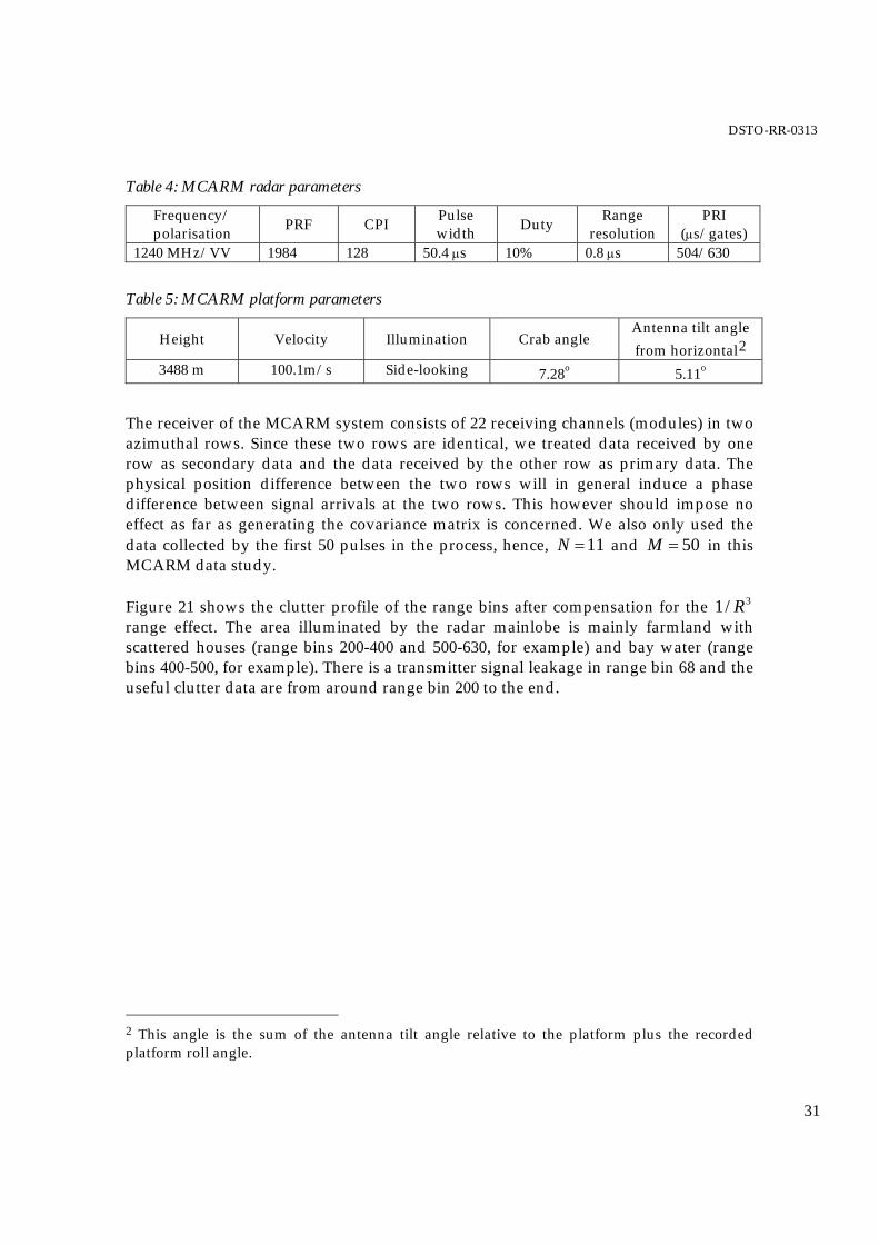
Table 4: MCARM radar parameters

Frequency/ polarisation PRF CPI Pulse

width Duty Range resolution

PRI (μs/gates)

1240 MHz/VV 1984 128 50.4 μs 10% 0.8 μs 504/630

Table 5: MCARM platform parameters

Height Velocity Illumination Crab angle Antenna tilt angle from horizontal2

3488 m 100.1m/s Side-looking 7.28o 5.11o

The receiver of the MCARM system consists of 22 receiving channels (modules) in two azimuthal rows. Since these two rows are identical, we treated data received by one row as secondary data and the data received by the other row as primary data. The physical position difference between the two rows will in general induce a phase difference between signal arrivals at the two rows. This however should impose no effect as far as generating the covariance matrix is concerned. We also only used the data collected by the first 50 pulses in the process, hence, 11=N and 50=M in this MCARM data study.

Figure 21 shows the clutter profile of the range bins after compensation for the 3/1 R range effect. The area illuminated by the radar mainlobe is mainly farmland with scattered houses (range bins 200-400 and 500-630, for example) and bay water (range bins 400-500, for example). There is a transmitter signal leakage in range bin 68 and the useful clutter data are from around range bin 200 to the end.

2 This angle is the sum of the antenna tilt angle relative to the platform plus the recorded platform roll angle.

DSTO-RR-0313

32

-40

-20

0

20

40

60

0 100 200 300 400 500 600

Range gate

Clu

tter (

dB)

Figure 21: Clutter profile against range after the 3/1 R range effect is compensated.

A moving target at range bin 299 has been detected and reported previously (Dong, 2005). Range cells 289 to 309 were, therefore, excluded in the secondary data for either the fixed window or sliding window processing.

A fixed window consisting of range cells 200 to 630 but excluding 289 to 309 was first used to sample uR for MF processing and fR for PAMF processing. The results are shown in Figure 22 to Figure 24. Both processes are able to detect the target at range bin 299. Overall, on average, the noise floor of the MF MDTS result is lower. It is also worth noting that the MF detection profile of signal versus range (Figure 23 (a)) in general follows the clutter profile (Figure 21) whereas the pattern of the PAMF MDTS (Figure 23 (b)) does not show such a feature.

DSTO-RR-0313

33

(a) MF MDTS

(b) PAMF MDTS, 5=p

Figure 22: Signal level versus range and Doppler processed by MF MDTS and PAMF MDTS using a fixed window of 200:630 with an exclusion of 289:309.

MF MDTS

PAMF MDTS, 5=p

Figure 23: Signal level versus range processed by MF MDTS and PAMF MDTS using a fixed window of 200:630 with an exclusion of 289:309.

DSTO-RR-0313

34

MF MDTS

PAMF MDTS, 5=p

Figure 24: Signal level versus range and Doppler processed by MF MDTS and PAMF MDTS using a fixed window of 200:630 with an exclusion of 289:309.

The DTS results are shown in Figure 25. We can see from the figure that both MF and PAMF do not sufficiently suppress the clutter, which would significantly increase the false alarm rate should the conventional DTS be used.

MF MDTS

PAMF MDTS, 5=p

Figure 25: MF DTS and PAMF DTS processes produce many spikes at the mainlobe clutter Doppler frequency deteriorating the detection performance.

Our next intention is to examine PAMF with reduced secondary data. It is better to use iid samples for such an intention. The consecutive range cells of MCARM data may not be iid samples as the data were also oversampled. The LFM bandwidth of the MCARM system was 1MHz, resulting in that the range sample rate corresponding the range resolution should be sμ0.1 whereas the actual range sample rate was sμ8.0 (see Table

DSTO-RR-0313

35

4). Therefore, non-consecutive range samples with an interval of 2 may be considered as iid samples.

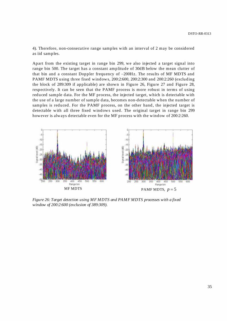
Apart from the existing target in range bin 299, we also injected a target signal into range bin 500. The target has a constant amplitude of 30dB below the mean clutter of that bin and a constant Doppler frequency of −200Hz. The results of MF MDTS and PAMF MDTS using three fixed windows, 200:2:600, 200:2:300 and 200:2:260 (excluding the block of 289:309 if applicable) are shown in Figure 26, Figure 27 and Figure 28, respectively. It can be seen that the PAMF process is more robust in terms of using reduced sample data. For the MF process, the injected target, which is detectable with the use of a large number of sample data, becomes non-detectable when the number of samples is reduced. For the PAMF process, on the other hand, the injected target is detectable with all three fixed windows used. The original target in range bin 299 however is always detectable even for the MF process with the window of 200:2:260.

MF MDTS

PAMF MDTS, 5=p

Figure 26: Target detection using MF MDTS and PAMF MDTS processes with a fixed window of 200:2:600 (exclusion of 389:309).

DSTO-RR-0313

36

MF MDTS

PAMF MDTS, 5=p

Figure 27: Target detection using MF MDTS and PAMF MDTS processes with a fixed window of 200:2:300 (exclusion of 289:300).

MF MDTS

PAMF MDTS, 5=p

Figure 28: Target detection using MF MDTS and PAMF MDTS processes with a fixed window of 200:2:260.

Finally the results of PAMF MDTS, with the use of sliding windows of 50 and 30 non-consecutive samples, are shown in Figure 29. It shows again that compared to the results of the fixed windows shown in Figure 27 and Figure 28, there is no improvement in terms of target detection, although a significant amount of additional computation is needed for implementation of the sliding window.

DSTO-RR-0313

37

(a) PAMF MDTS, 5=p , with a sliding window of 50 non-consecutive samples

(b) PAMF MDTS, 5=p , with a sliding window of 30 non-consecutive samples

Figure 29:Target detection using the PAMF MDTS process with a sliding window of (a) 50 non-consecutive samples and (b) 30 non-consecutive samples.

5.4 Conclusions The performance of the PAMF approach has been assessed in this Section using three types of radar data. The results of the conventional MF method have served as benchmarks in the assessment. Based on the results, we have observed the following points:

• MF outperforms PAMF if sample data are ample. • PAMF is much more robust if sample data are limited. • The sliding window processing does not seem to show a better detection

performance, and the fixed window processing is satisfactory and very computationally efficient.

• The conventional DTS by the inclusion of numerically unstable data in the clutter notch can produce false alarms and a modified version (MDTS) generally outperforms the conventional DTS.

Operational counts for the PAMF algorithm and its computational savings compared to the conventional MF algorithm are discussed in the next Section.

6. Estimation of Operational Counts This section estimates operational counts (ops) for the MF and PAMF algorithms. In the estimation, we only count complex multiplication/division, and ignore addition/subtraction. For simplicity we also assume that no special digital signal

DSTO-RR-0313

38

processing (DSP) hardware is used, so that all calculations are treated with the same weight. Special structures of matrices such as complex conjugate, which often lead to special algorithms to save ops, are also not considered. For instance, the number of ops for a matrix multiplication BCA = is lmn where nm×∈A , lm×∈Β and nl×∈C .

Ops required for the MF and PAMF algorithms are listed in Table 6 and Table 7, respectively.

Table 6: Ops required for the MF process.

Algorithm Task Reference Eqn

Ops

)1(MFC ∑==

K

k

Hkku

1

ˆ xxR (36) 2)(MNK

)2(MFC 1ˆ −uR (1) 3)(MN

)3(MFC eRw 1ˆ −= uMF (1) 2)(MN )4(MFC ew H

MFMF =Λ 0 (9) MN

)5(MFC

0

2|

MF

HMF

MF Λ=Λ

xw|

(9) MN

Note that the actual ops for )1(MFC may be reduced by a half, if we take account of the

Hermitian structure of uR̂ . Similarly, the ops required for )2(MFC may be reduced by

a half as 1ˆ −uR is also Hermitian. The ops required for the inverse of a matrix are justified

by Isaacson and Keller (1966).

DSTO-RR-0313

39

Table 7: Ops required for the PAMF process.

Algorithm Task Reference Eqn

Ops

)1(PAMFC fR̂ (35) and (36)

)]()([ 222 pMpMMKN −+−−

)2(PAMFC fA (32) 323)( NppN + )3(PAMFC T (37) and

(39) 32 ]1)1()1[( Npp ++++

)4(PAMFC u (40) )(2 pMpN − )5(PAMFC s (40) )(2 pMN − )6(PAMFC ε (40) )(2 pMpN − )7(PAMFC ν (40) )(2 pMN − )8(PAMFC ssH

PAMF =Λ 0 (40) )( pMN −

)9(PAMFC

0

2

PAMF

H

PAMF Λ=Λ

|νs|

(40) )( pMN −

In the MF process assuming the Doppler resolution used in Algorithm )3(MFC is

)2/(1 M (normally the number of Doppler bins is equal to M ), we need M2 repetitions of )3(MFC , )4(MFC and )5(MFC in searching for possible target signals with unknown Doppler frequencies and amplitudes in a single range cell. If we use a fixed window for sampling uR̂ the total ops for processing a segment of rgK range cells collected by a CPI are,

)5(2)]4()3([2)2()1( MFrgMFMFMFMFMF MCKCCMCCC ++++= (54)

Similarly assuming that the Doppler resolution used in calculation for the PAMF processing is )2/(1 M , and a fixed window is used for sampling fR̂ , then the total ops

for processing a segment of rgK range cells collected by a CPI are,

)9(2)]7()6([)]8()5()4([2)3()2()1(

PAMFrgPAMFPAMFrg

PAMFPAMFPAMFPAMFPAMFPAMFPAMF

MCKCCKCCCMCCCC

++++++++=

(55)

Shown in Figure 30 is the ratio of the PAMF ops to the MF ops, which is a function of the number of pulses M , the number of antenna channels N and the number of range cells rgK . The other two parameters used in the calculation include 50=K and 5=p .

DSTO-RR-0313

40

The fixed window processing is assumed. It can be seen that the computational savings of the PAMF process varies with parameters. For a case where M and N are large, and rgK small, the computational advantage of the PAMF process is significant. On

the other hand, if M and N are small, and rgK large, there is not much

computational advantage in the PAMF process. This is because when rgK is small, the

ops for the inversion of uR̂ is dominant in the MF processing. However with an

increase in rgK , the portion for computing the inverse of uR̂ in the whole process becomes less dominant.

DSTO-RR-0313

41

0

20

40

60

80

100

0 8 16 24 32 40 48 56 64

Number of pulses (M)

Rat

io o

f PA

MF

ops

to M

F op

s (%

)N = 10

N = 20

N = 30

(a) 100=rgK

0

20

40

60

80

100

0 8 16 24 32 40 48 56 64

Number of pulses (M)

Rat

io o

f PAM

F op

s to

MF

ops

(%)

N = 10

N = 20

N = 30

(b) 500=rgK

Figure 30: Ratio of the PAMF ops to the MF ops, as a function of the number of pulses M , the number of antenna channels N and the number of range cells rgK .

Ops required by the MF and PAMF processes are shown in Figure 31. It shows the amount of ops even for the PAMF process is still huge, considering the time frame for a CPI to be in a scale of milliseconds for airborne radars. Therefore how to further reduce ops will still be an active research area in the future. The figure also shows that for the same process, an increase in the number of range cells to be processed does not incur a significant increase of ops. Therefore, using a fixed window to process a large chunk of range cells should be a preferable option.

DSTO-RR-0313

42

1.E+06

1.E+07

1.E+08

1.E+09

1.E+10

10 30 50 70

Number of pulses (M)

Ops

requ

ired

MF, N = 10

MF, N = 30

PAMF, N = 10

PAMF, N = 30

(a) 100=rgK

1.E+06

1.E+07

1.E+08

1.E+09

1.E+10

10 30 50 70

Number of pulses (M)

Ops

requ

ired

MF, N = 10

MF, N = 30

PAMF, N = 10

PAMF, N = 30

(b) 500=rgK

Figure 31: Ops required for the MF and PAMF processes.

7. PAMF with Combined Forward and Backward Coefficients

One of the problems of the PAMF method is the dimensionality loss mentioned in Section 3. Using the thp order AR parameters )(kH

fA , pk ,,1L= , we can only

estimate { }1,,1,)(ˆ −+= Mppnn Lx from the original data sequence

{ }1,,1,0)( −= Mnn Lx . It means that the original M -point time sequence now becomes an )( pM − -point time sequence. As we know that both the Doppler resolution and processing gain are proportional to the number of points in a time

DSTO-RR-0313

43

sequence, the dimensionality reduction directly results in a loss in the Doppler resolution and processing gain. The impact can be small or significant depending on the values of M and p . In the case where the ratio of MpM /)( − is small, the impact can be significant.

Equation (14) is a process of the forward linear prediction which estimates the sequence { }1,,1,)(ˆ −+= Mppnn Lx . The sequence { }1,,1,0)(ˆ −= pnn Lx , which cannot be estimated using the forward linear prediction, however, may be estimated with the use of the backward linear prediction as (Marple, Jr, 1987),

∑ +−==

p

k

Hb knkn

1)()()(ˆ xAx 1,,1,0 −= pn L (56)

where )(kHbA , pk ,,1L= , are backward prediction parameters. Together with the

forward prediction given in (14), we now have a full dimension of the linear prediction residual as,

⎪⎩

⎪⎨

⎧

−+=∑ −

−=∑ +=−=

=

=

1,,1,)()(

1,,1,0)()()(ˆ)()(

0

0

Mppnknk

pnknknnn p

k

Hf

p

k

Hb

L

L

xA

xAxxε (57)

The remaining process is the same and there is no need to repeat it here except to define the estimates of the backward parameters, )(kbA , pk ,,1L= . In order to find these parameters, we need to find the minimum squared residual given by (58),

∑+∑=−

=

−

=

11

0)()(min)()(min}min{

M

pn

Hp

n

HH nnnn εεεεεε (58)

The function }min{ εεH in (58) is expressed as the sum of two terms indicating that the backward parameters and forward parameters are uncorrelated and can be separately determined. The estimate of the forward parameters given in (32) therefore remains unchanged. The estimate of the backward parameters is given below as (following a similar mathematical manipulation),

⎥⎥⎥

⎦

⎤

⎢⎢⎢

⎣

⎡

−=

⎥⎥⎥⎥⎥⎥

⎦

⎤

⎢⎢⎢⎢⎢⎢

⎣

⎡

=−

01

)(

)1(

)0(

bbb

N

b

b

b

b

pRR

I

A

A

A

AM

(59)

DSTO-RR-0313

44

where pNpNbb

×∈R and NpNb

×∈0R are sub-block matrices of NpNpb

)1()1( +×+∈R given as,

∑ +=⎥⎥⎦

⎤

⎢⎢⎣

⎡=

−

=

1

00

000):(

p

ku

bbb

bb pkkR

RR

RRR (60)

It is worth noting that the order of bA in (59) is from low to high, contrary to the order of fA in (32) which is from high to low. Also the divisions of the sub-block matrices in

(33) and (60) used for computing fA and bA , respectively, are different.

The manipulation matrix B given in (20) should be modified accordingly to include the backward prediction as,

⎥⎥⎥⎥⎥⎥⎥⎥⎥⎥⎥⎥

⎦

⎤

⎢⎢⎢⎢⎢⎢⎢⎢⎢⎢⎢⎢

⎣

⎡

=

NHf

NHf

NHf

HbN

HbN

HbN

p

pp

p

pp

IA

IAIA

AI

AIAI

B

L

O

L

L

L

O

L

L

)(

)()(

)(

)()(

(61)

Similarly the corresponding mean temporal residual covariance matrix is given as,

⎥⎥

⎦

⎤

⎢⎢

⎣

⎡

⊗

⊗=

− ε

εε

fpM

bp

RI

RIR (62)

where

∑ ==−

=

1

0

1)(1 p

nbb

Hbb p

np

ARARR εε (63)

Aimed at avoiding the dimensionality loss problem we have modified the PAMF algorithm using both the forward and backward predictions to maintain the dimensionality of the time sequence. The above formulation uses p points of

DSTO-RR-0313

45

backward prediction and pM − points of forward prediction. Obviously we can form other combinations if desired. We could select a combination containing a maximum number of points including pM − points of backward prediction and pM − points of forward prediction, for instance. However, according to the linear algebra, the maximum number of independent vectors after a linear transform is no greater than the original number of the independent vectors. Therefore, we do not expect that there would exist a combination which contains more independent vectors than the original.

To view the impact on the Doppler resolution and the processing gain due to the dimensionality reduction of PAMF, the example shown in Figure 4 is re-examined. To clearly show the impact we have chosen 10=M and 5=p . The results are shown in Figure 32. The Doppler resolution of PAMF with forward prediction for this example is only a half of the Doppler resolution of the conventional STAP, since the PAMF process loses 50% of the time sequence. On the other hand we see the resolution of the PAMF with both backward and forward predictions is the same as that of the STAP, because of no dimensionality loss of the algorithm. A 3dB loss in the signal peak level for the process of the PAMF with forward prediction only is also observed.

-30

-20

-10

0

10

20

30

-150 -100 -50 0 50 100 150

Doppler frequency (Hz)

Sign

al le

vel (

dB)

PAMF, fw d only

PAMF, fw d and bw d

STAP

Figure 32: Doppler resolution comparison between the PAMF with forward prediction and the PAMF with both backward and forward predictions. The STAP result is also shown as a benchmark.

As the ratio of MpM /)( − increases, the impact of the dimensionality loss fades. The detection results for target 1 in the RLSTAP dataset is plotted in Figure 33. In this example the values of 31=M and 5=p result in a 16% decrease in the Doppler resolution if the PAMF with forward prediction is used.

DSTO-RR-0313

46

-50

-40

-30

-20

-10

0

-1000 -750 -500 -250 0 250 500 750 1000

Doppler frequency (Hz)

Sig

nal l

evel

(dB

)

PAMF fwd onlyPAMF fwd and bwdSTAP

Figure 33: The impact of the dimensionality loss on the Doppler resolution and processing gain fades as the ratio of MpM /)( − increases. Shown is the target detection of target 1 in the RLSTAP dataset with 31=M and .5=p

8. Summary Much research effort, notably that carried out and sponsored by AFRL, has been made in developing and evaluating the PAMF approach for the last decade. This report has traced, analysed and evaluated this technique in great detail. Accessible publications of PAMF often omit details of the mathematics due to space limitation, making the papers difficult to follow. This report therefore has independently provided full mathematical derivation for a full understanding of the algorithm. The performance of the approach has then been assessed using three different types of data, namely data generated using a simple generic radar model, data generated by high fidelity radar simulation software, RLSTAP, and real radar data collected by the MCARM system. In the assessment, the results of the conventional space-time MF process have been used as benchmarks for comparison. The ops for the approach have also been estimated and computational savings of PAMF in comparison to the MF algorithm have been given. Finally a modification to the PAMF approach is proposed. The modified PAMF uses both the forward and backward prediction parameters to maintain the dimensionality of the process, so that the Doppler resolution and processing gain is maintained.

Based on the study, the PAMF algorithm has two advantages over the conventional MF algorithm:

• The ops requirement is less. Computational savings, compared to the MF algorithm, vary from less than 20% for a system with a small number of pulses

DSTO-RR-0313

47

M and a small number of channels N , and a large number of range bins rgK ,

to more than 90% for a system with large M and N , and small rgK . • The PAMF algorithm is much more robust than the MF algorithm in the case

where the set of sample data is small.

Problems of the PAMF process include

• If PAMF uses the forward prediction parameters only, the equivalent temporal independent measurements are reduced from M to pM − ( p is the order of the filter, and M is the number of pulses in a CPI), which in turn reduces the Doppler resolution and the processing gain. The impact can be significant if the ratio of MpM /)( − is small. However, as proposed, if PAMF is formed using both the forward and backward prediction, there is not a loss in dimensionality.

• The output of the PAMF MDTS processing does not seem to follow the pattern of the original clutter profile whereas the MF MDTS does (see Figure 23 and Figure 21). Whether this imposes a problem to target detection warrants a further investigation.

All simulations have suggested that using the sliding widow architecture to sample the covariance matrix for each range bin does not statistically improve results. Therefore a preferable option is to use the fixed window architecture to sample the covariance matrix and process a block of range bins, which significantly saves computational cost.

Overall the amount of ops required for the PAMF algorithm is still huge considering the time frame available for airborne radars. How to further reduce ops demand in processing phased array data warrants future research.

9. Acknowledgement The Rome Laboratory, Air Force Material Command supplied the MCARM data and the RLSTAP software. Mr A Mahoney generated the RLSTAP data. Comments of Drs P Berry and J Whitrow in the vetting process are also acknowledged.

10. References Brennan, L E, and Staudaher, F M, “Subclutter visibility demonstration”, Technical Report, RL-TR-92-21, Adaptive Sensors Incorporated, March 1992.

Bresler, Y, “Maximum likelihood estimation of a linearly structured covariance with application to antenna array processing”, Proceedings of the Fourth Annual ASSP Workshop on Spectrum Estimation and Modelling, pp. 172-175, 3-5 Aug 1988.

DSTO-RR-0313

48

Carlson, B D, “Covariance matrix estimation erroes and diagonally loading in adaptive arrays,” IEEE Trans on Aerospace and Electronic Systems, vol. 24, no. 4, pp. 397-401, 1988.

Compton, Jr, R T, Adaptive antennas, concepts and performance, Prentice Hall, 1988.

Dong, Y, “Approximate invariance of the inverse of the covariance matrix and the resultant pre-built STAP processor”, Research Report, DSTO-RR-0291, DSTO, 2005.

Fenner, D, and Hoover, W F, “Test results of a space-time adaptive processing system for airborne early warning radar”, Proceedings of IEEE 1996 National Radar Conference, Ann Arbor, Michigan, 13-16 May 1996.

Gerlach, K, and Picciolo, M L, “Airborne/spacebased radar STAP using a structured covariance matrix”, IEEE Trans on Aerospace and Electronic Systems, vol. 39, no. 1, pp. 269-281, 2003.

Isaacson, E, and Keller, H B, Analysis of Numerical Methods, John Willey & Sons, Inc, 1966.

Klemm, R K, Principles of space-time adaptive processing, 2nd edn, IEE, 2002.

Marple, Jr, S L, Digital Spectral Analysis with Applications, Prentice-Hall Inc, 1987.

Michels, J R, Roman, J R, and Himed, B, “Beam control using the parametric adaptive matched filter STAP approach”, Proceedings of IEEE Radar Conference 2003, pp. 405-412.

MITRE, “STAP processing monostatic and bistatic MCARM data”, Final report prepared by MITRE, Centre for Air Force C2 Systems, Bedford, MA, 1999.

RAFDCI, “MCARM/STAP data analysis”, Final report, Part I and II, prepared by Research Associates for Defence Conversion Inc., New York, 1999.

Rangaswamy, M, and Michels, J H, “A parametric multichannel detection algorithm for correlated non-Gaussian random processes”, Proceedings of 1977 IEEE National Radar Conference, pp. 349-354, Syracuse, NY, 13-15 May.

Rangaswamy, M, Michels, J H, and Weiner, D D, “Multichannel detection for correlated non-Gaussian random processes based on innovations”, IEEE Trans on Signal Processing, vol. 43, no. 8, pp. 1915-1922, 1995.

Reed, I S, Mallett, J D, and Brennan, L E, “Rapid convergence rate in adaptive arrays”, IEEE Trans on Aerospace and Electronic Systems, vol. AES-10, no. 6, 1974.

DSTO-RR-0313

49

Robey, F C, Fuhrmann, D R, Kelly, E J, and Nitzberg R, “A CFAR adaptive matched filter detector”, IEEE Trans on Aerospace and Electronic Systems, vol. 28, no. 1, pp. 208-216, 1992.

Roman, J R, Davis, D W, and Michels, J H, “Multichannel parametric models for airborne phased array clutter”, Proceedings of 1977 IEEE National Radar Conference, pp. 72-77, Syracuse, NY, 13-15 May.

Roman, J R, Rangaswamy, M, Davis, D W, Zhang, Q, Himed, B, and Michels, J H, “Parametric adaptive matched filter for airborne radar applications”, IEEE Trans on Aerospace and Electronic Systems, vol. 36, no. 2, pp. 677-692, April 2000.

Sarkar, T K, Wang, H, Park, S, Adve, R, Koh, J, Kim, K, Zhang, Y, Wicks, M C, and Brown, R D, “A deterministic least-squares approach to space-time adaptive processing”, IEEE Trans on Antennas and Propagation, vol. 49, no. 1, January 2001.

Sloper, D, Fenner, D, Arntz, J, and Fogle, E, “Multi-channel airborne radar measurement (MCARM), MCARM flight test”, Westinghouse Electronic Systems, Final Technical Report, RL-TR-96-49, vol. 1, April 1996.

Steiner, M, and Gerlach, K, “Fast converging adaptive processor or a structured covariance matrix”, IEEE Trans on Aerospace and Electronic Systems, vol. 36, no. 4, pp. 1115-1126, 2000.

Steiner, M, and Gerlach, K, “Fast converging maximum-likelihood interference cancellation,” Proceedings of IEEE 1998 National Radar Conference, pp. 117-122, Dallas, TX, 12-13 May 1998.

Van Trees, H L, Optimum Array Processing, Part IV, of Detection, Estimation and Modulation Theory, Wiley Interscience, 2002.

Wang, H, and Cai, L, “On adaptive spatial-temporal processing for airborne surveillance radar systems”, IEEE Trans on Aerospace and Electronic Systems, vol. 30, no. 3, pp. 660-670, 1994.

Wang, Y L, Chen, J W, Bao, Z, and Peng, Y N, “Robust space-time adaptive processing for airborne radar in nonhomogeneous clutter environments”, IEEE Trans on Aerospace and Electronic Systems, vol. 39, no. 1, pp. 70-81, 2003.

Ward, J, “Space-time adaptive processing for airborne radar”, Technical Report TR-1015, Lincoln Laboratory, MIT, 1994.

Ward, J, and Kogon, S M, “Space-time adaptive processing (STAP) for AMTI and GMTI radar”, tutorial slides, CD of the Proceedings of 2004 IEEE Radar Conference, Philadelphia Pennsylvania, 26-29 April 2004.

51

Parametric Adaptive Matched Filter and its Modified Version

Yunhan Dong

(DSTO-RR-0313)

AUSTRALIA DEFENCE ORGANISATION No. of copies

Task Sponsor, DCEO-DMO 1 printed

S&T Program Chief Defence Scientist Deputy Chief Defence Scientist Policy AS Science Corporate Management Director General Science Policy Development

1 1 1 1

Counsellor Defence Science, London Doc Data Sheet Counsellor Defence Science, Washington Doc Data Sheet Scientific Adviser to MRDC, Thailand Doc Data Sheet Scientific Adviser Joint 1 Navy Scientific Adviser 1 Scientific Adviser – Army 1 AirForce Scientific Adviser 1 Scientific Adviser to the DMO 1

Platforms Sciences Laboratory Deputy Chief Defence Scientist Aerospace

Doc Data Sht & Exec Summ

Systems Sciences Laboratory

EWSTIS (soft copy for accession to EWSTIS Web site) 1 Chief, Electronic Warfare and Radar Division Doc Data Sht & Dist List Research Leader, Maritime EW Doc Data Sht & Dist List Research Leader, Air EW Doc Data Sht & Dist List Research Leader, JIL EW Doc Data Sht & Dist List Research Leader, Microwave Radar Doc Data Sht & Dist List Head, ES Systems Doc Data Sheet Head, RF Countermeasures Doc Data Sheet Head, RF Technology Doc Data Sheet Head, Strategic and Land EW Doc Data Sheet Head, Aerospace Systems Doc Data Sheet Head, Maritime Systems Doc Data Sheet Head, EO Countermeasures Doc Data Sheet Head, EO Technology Doc Data Sheet Head, Radar Systems and Technologies Doc Data Sheet Head, Maritime Air Surface Doc Data Sheet Head, Maritime Surface Radar Doc Data Sheet Head, Radar Signatures Doc Data Sheet

}

DSTO-RR-0313

52

Task Manager: Scott Capon, EWRD 1 printed Yunhan Dong, EWRD 1 printed

DSTO Library and Archives

Library Edinburgh 1 printed + Doc Data Sheet Defence Archives 1 printed Library Canberra Doc Data Sheet

Capability Development Group

Director General Maritime Development Doc Data Sheet Director General Land Development 1 Director General Capability and Plans Doc Data Sheet Assistant Secretary Investment Analysis Doc Data Sheet Director Capability Plans and Programming Doc Data Sheet Director General Australian Defence Simulation Office Doc Data Sheet

Chief Information Officer Group

Director General Australian Defence Simulation Office Doc Data Sheet AS Information Strategy and Futures Doc Data Sheet

Strategy Group

Director General Military Strategy Doc Data Sheet Assistant Secretary Governance and Counter-Proliferation Doc Data Sheet

Navy

Maritime Operational Analysis Centre, Building 89/90 Garden Island Sydney NSW

Deputy Director (Operations) Deputy Director (Analysis)

Doc Data Sht & Dist List

Director General Navy Capability, Performance and Plans, Navy Headquarters

Doc Data Sheet

Director General Navy Strategic Policy and Futures, Navy Headquarters

Doc Data Sheet

Air Force SO (Science) - Headquarters Air Combat Group, RAAF Base,

Williamtown NSW 2314 Doc Data Sht & Exec Summ

Army ABCA National Standardisation Officer

Land Warfare Development Sector, Puckapunyal e-mailed Doc Data Sheet

SO (Science) - Land Headquarters (LHQ), Victoria Barracks NSW Doc Data Sht & Exec Summ SO (Science), Deployable Joint Force Headquarters (DJFHQ) (L), Enoggera QLD

Doc Data Sheet

Joint Operations Command Director General Joint Operations Doc Data Sheet

DSTO-RR-0313

53

Chief of Staff Headquarters Joint Operations Command Doc Data Sheet Commandant ADF Warfare Centre Doc Data Sheet Director General Strategic Logistics Doc Data Sheet COS Australian Defence College Doc Data Sheet

Intelligence and Security Group AS Concepts, Capability and Resources 1 DGSTA , DIO 1 Manager, Information Centre, Defence Intelligence Organisation 1

Defence Materiel Organisation Deputy CEO Doc Data Sheet Head Aerospace Systems Division Doc Data Sheet Head Maritime Systems Division Doc Data Sheet Program Manager Air Warfare Destroyer Doc Data Sheet

OTHER ORGANISATIONS National Library of Australia 1 NASA (Canberra) 1

UNIVERSITIES AND COLLEGES

Australian Defence Force Academy Library Head of Aerospace and Mechanical Engineering

1 1

Hargrave Library, Monash University Doc Data Sheet

OUTSIDE AUSTRALIA

INTERNATIONAL DEFENCE INFORMATION CENTRES

US Defense Technical Information Center 1 UK Dstl Knowledge Services 1 Canada Defence Research Directorate R&D Knowledge & Information Management (DRDKIM)

1

NZ Defence Information Centre 1

ABSTRACTING AND INFORMATION ORGANISATIONS Library, Chemical Abstracts Reference Service 1 Engineering Societies Library, US 1 Materials Information, Cambridge Scientific Abstracts, US 1 Documents Librarian, The Center for Research Libraries, US 1

INFORMATION EXCHANGE AGREEMENT PARTNERS

National Aerospace Laboratory, Japan 1 National Aerospace Laboratory, Netherlands 1

DSTO-RR-0313

54

SPARES

5 printed

Total number of copies: 38 Printed: 10 PDF: 28

DSTO-RR-0313

Page classification: UNCLASSIFIED

DEFENCE SCIENCE AND TECHNOLOGY ORGANISATION

DOCUMENT CONTROL DATA 1. PRIVACY MARKING/CAVEAT (OF DOCUMENT)

2. TITLE Parametric Adaptive Matched Filter and its Modified Version

3. SECURITY CLASSIFICATION (FOR UNCLASSIFIED REPORTS THAT ARE LIMITED RELEASE USE (L) NEXT TO DOCUMENT CLASSIFICATION)

Document (U) Title (U) Abstract (U)

4. AUTHOR(S) Yunhan Dong

5. CORPORATE AUTHOR Defence Science and Technology Organisation PO Box 1500 Edinburgh SA 5111

6a. DSTO NUMBER DSTO-RR-0313

6b. AR NUMBER AR-013-643

6c. TYPE OF REPORT Research Report

7. DOCUMENT DATE May 2006

8. FILE NUMBER 20006/1060092

9. TASK NUMBER AIR 05/264

10. TASK SPONSOR DCEO-DMO

11. NO. OF PAGES 70

12. NO. OF REFERENCES 38

13. URL on the World Wide Web http://www.dsto.defence.gov.au/corporate/reports/DSTO-RR-0313.pdf

14. RELEASE AUTHORITY Chief, Electronic Warfare and Radar Division

15. SECONDARY RELEASE STATEMENT OF THIS DOCUMENT Approved for Public Release OVERSEAS ENQUIRIES OUTSIDE STATED LIMITATIONS SHOULD BE REFERRED TO DOCUMENT EXCHANGE, PO BOX 1500, EDINBURGH, SA 5111, AUSTRALIA 16. DELIBERATE ANNOUNCEMENT

No Limitations

17. CASUAL ANNOUNCEMENT Yes 18. DSTO RESEARCH LIBRARY THESAURUS Adaptive filters Airborne radar Space-time adaptive processing Mathematical analysis 19. ABSTRACT The parametric adaptive matched filter (PAMF) for space-time adaptive processing (STAP) has been an interesting research area in the airborne radar data processing community over the last decade. Starting from providing a complete formulation of PAMF, this report assesses the performance of PAMF using simulated data as well as real airborne data collected by the Multi-channel Airborne Radar Measurements (MCARM) system with use of results from the conventional STAP as a benchmark. A modified PAMF approach using both forward and backward predictions is proposed to eliminate the dimensionality loss of the method. Finally the operational counts and computational savings of PAMF are also estimated.

Page classification: UNCLASSIFIED