paramagnetic–ferrimagnetic transition in strong coupling paramagnetic systems: effect of cubic...

Journal of Magnetism and Magnetic Materials 234 (2001) 153–173

Paramagnetic–ferrimagnetic transition in strong couplingparamagnetic systems: effect of cubic anisotropy interaction

M. Chahid, M. Benhamou*

Laboratoire de Physique des Polym "eeres et Ph !eenom "eenes Critiques, Facult !ee des Sciences Ben M’sik, B.P. 7955, Casablanca, Morocco

Received 17 November 2000; received in revised form 2 March 2001

Abstract

The purpose of the present work is a quantitative investigation of the biquadratic exchange interaction effects on theparamagnetic–ferrimagnetic transition arising from two strongly coupled paramagnetic (1-spin) sublattices, ofrespective moments m andM. The free energy describing the physics of the system is of Landau type. In addition to the

quadratic and quartic terms, in both m and M, this free energy involves two mixing interaction terms. The first is alowest order coupling �CmM, where C50 stands for the coupling constant measuring the interaction between the twosublattices. While the second, which is relevant for 1-spin systems and which traduces the dipole–dipole (or biquadratic)

interaction, is of type wm2M2, where w > 0 is the new coupling constant. These two interactions enter in competition,and then, they induce drastic changes of the magnetic behavior of the material. The main change is that, the presence ofthis high order coupling tends to destroy the ferrimagnetic order of the system. We first show that the introduction of

this biquadratic interaction does not affect the values of critical exponents. Also, we find that the compensationtemperature (when it exists) and the compensation magnetic field are shifted to their lowest values, in comparison withthe w ¼ 0 case. The Arrott-phase-diagram shape is also investigated quantitatively. We show the existence of threeregimes depending on the values of w. When the latter is small, we find that the region of competition between the

coupling C and the applied magnetic field H becomes more narrow under the effect of w (by competition, we mean thepassage from the antiparallel state to the parallel one). While for higher values of w, this competition disappearscompletely, and then, the system loses its ferrimagnetic character. Kinetics of the phase transition is also examined,

when the temperature is lowered from an initial value Ti to a final one Tf very close to the critical temperature Tc. As inthe w ¼ 0 case, we find that kinetics is controlled by two kinds of relaxation times t1 and t2. The former is the relevanttime, and is associated to long-wavelength fluctuations driving the system to undergo a phase transition. The second is a

short time, which controls local dynamics. Near Tc, we show that, in particular, the longest relaxation time t1 becomesless important in comparison with that relative to the w ¼ 0 case. Finally, we note that the existence of two relaxationtimes is consistent with the predictions of a recent experiment, which was concerned with the 1/2-spin compounds

LixNi2�xO2, where the composition x is close to 1. # 2001 Elsevier Science B.V. All rights reserved.

PACS: 05.70.Fh; 75.50.Gg; 05.20.Dd

Keywords: Sublattices; Cubic anisotropy; Paramagnetism; Ferrimagnetism; Transition; Relaxation time

*Corresponding author. Tel.: +212-2-704672; fax: +212-2-704675.

E-mail address: [email protected] (M. Benhamou).

0304-8853/01/$ - see front matter # 2001 Elsevier Science B.V. All rights reserved.

PII: S 0 3 0 4 - 8 8 5 3 ( 0 1 ) 0 0 1 9 8 - 6

1. Introduction

Super-weak ferrimagnetism arising from an important class of magnetic materials are the subject of agreat deal of attention from theoretical and experimental points of view. Among these, we can quote, first,the Heusler alloys [1] based on the composition X2YZ with X=Pd, Cu, Y=Ti, V and Z=Al, In, Sn, andsecond, the lamellar Curie–Weiss paramagnetic compounds [2], like AMxM

01�xO2 04x51ð Þ with A=Li,

Na, K ....; M, M0 ¼ N, Co, .... Because of their very high cell voltage (in the 3.5–4V range), the lattercompounds are promising for interesting applications, especially in the domain of energy stocking (long lifelithium batteries) [3–5]. In particular, LiNiO2 and LiCoO2 have attracted the attention of researchers inlithium battery field, because of their high cathode potential versus Li=Liþ electrode and good reversibilityat Li-doping/undoping [6].From the magnetic point of view, such systems are made of two strongly coupled paramagnetic

sublattices of Pauli or Curie–Weiss types [7,8], of respective magnetic moments m and M. To under-stand the origin of the existence of these sublattices, consider the LiNiO2-compound as a typical example. Itis very difficult to know the stoichiometric phase of LiNiO2. As a matter of fact, magnetic and densitymeasurements showed that the lithium deficiency is not due only to Liþ-ions vacancies in the lithiumlayers, but to the presence of excess nickel occupying Liþ-ion sites [9]. The amount of displacedNi-ions is often expressed as z in the explicit formula: Liþ1�zNi

2þz

� �3ðbÞ Ni3þ1�zNi

2þz

� �3ðaÞO2. The

displacement of the Ni-ions in the lamellar compounds, from the octahedric sites of the Ni-layer tothose of the Li-layer, was widely confirmed by X-ray diffraction experiments [10,11] and by neutronscattering [2,11,12]. It is clear that the presence of Ni2þ-ions in the 3(a) and 3(b) sites is responsiblefor the existence of two coupled magnetic sublattices ðmÞ and ðMÞ. It is also assumed that the presence ofNi-ions has a tendency to prevent the diffusion of Li-ions in oxidation/reduction process, and then,it leads to a notable diminution of cathode capacity. We note that, not only the electrochemicalbehavior that are affected by the Ni-layer in the Li-Layer, but also the magnetic behavior of thecompound.To study the critical magnetic behavior of such materials, a continuous model based on the Landau

theory [13–15] was proposed, few years ago, by Neumann and coworkers [16]. Within the framework of thismodel, the para-ferrimagnetic transition arising from these materials was widely studied, applying, first, themean-field theory [16–19], and second, the Renormalization-Group techniques [20] as in the case of theusual para-ferromagnetic transitions [21–23]. According to this model, above the critical temperature Tcgreater than room temperature, the system is in the paramagnetic phase, where both moments m and Mvanish. Below Tc, an antiparallel configuration of these moments is favored, and then, a ferrimagnetic ordertakes place, with a non-vanishing overall magnetization Mtot ¼ mþM. The strong coupling between thetwo sublattices was taken into account introducing an extra coupling term �CmM in the free energy (seebelow). The coupling constant C that plays the role of an internal magnetic field is negative, ensures theanti-parallel alignment of magnetic moments m and M at low temperature. In addition, the free energyinvolves pure quartic terms in these moments, i.e. um4 and vM4 (u > 0 and v > 0 are the correspondingcoupling constants). It was established that the model is a good candidate to study the 1/2-spin materials.However, in the case of 1-spin systems, some additional biquadratic exchange coupling term, wm2M2,should be incorporated in the free energy (see below). Indeed, in their experimental study on theLixNi1� xO-compound [24], Goodenough and coworkers demonstrated the existence of a significantdipole–dipole interaction, which must affect the total configuration of atomic moments. The authors statedthat the system can be represented by formula LiþxNi

2þ1�2xNi

3þx O, and then, they suggested that the Ni2þ-ion

unambiguously has a spin S ¼ 1, and that, the Ni3þ-ion is probably in the low-spin state, i.e. S ¼ 1=2. Intheir analysis, it was assumed that for all compositions (at saturation), the magnetic moments in alternateð1 1 1Þ-planes are parallel, and anti-parallel to those in the neighboring ð1 1 1Þ-planes. The generalcompositional formula can be written as: ðLiþx�yNi

2þ0:5�x�zNi

3þzþyÞAðLi

þy Ni

2þ0:5�xþzNi

3þx�y�zÞBO, with 2y4x;

M. Chahid, M. Benhamou / Journal of Magnetism and Magnetic Materials 234 (2001) 153–173154

2z41� 2x. The brackets that represent the set of alternate ð1 1 1Þ-planes are coupled in anantiferromagnetic way, and then, they indicate two sublattices A and B.The natural question to ask here is how the critical magnetic behavior of such systems can be affected by

the presence of the dipole–dipole interaction wm2M2. The answer to this question is precisely the purpose ofthe present work, using mean-field theory.From a static point of view, such a new interaction is relevant for physics [25], and alters considerably the

Arrott phase-diagram and compensation point, for instance. We show, in particular, that the cubicanisotropy term wm2M2 is in competition with the bilinear interaction �CmM, and then, it has thetendency to destroy the ferrimagnetic order of the material. We determine the condition on the coupling wto have a region of competition between the coupling C and an external magnetic field H. This allows us toderive some temperature Tw depending on both C and w, above which the region of competition in theArrott phase-diagram becomes very narrow, and the system loses its ferrimagnetism. The compensationtemperature (when it exists) and compensation magnetic field are found to be shifted to their lowest values,in comparison with those relative to the w ¼ 0 case.The kinetics of phase transition is also investigated. The spin relaxation-time of the system, when the

temperature is changed from an initial value Ti to a final one Tf very close to Tc, is found to be governed, asin the w ¼ 0 case [19], by two kinds of relaxation-times t1 and t2. The former is a long-time associated withlong-wavelength fluctuations. This is the relevant time that drives the system to undergo a phase transition.The second is a short-time, which governs local dynamics. We find, in particular, that the relaxation-time t1remains smaller than the one with w ¼ 0, near the critical point.The remainder of this presentation proceeds as follows. In Section 2, we present the model. Investigation

of the mean-field critical behavior of the materiel is the aim of Section 3. We study, in Section 4, the effect ofthe presence of w on the compensation point. We present, in Section 5, results that dealt with the variationof the overall magnetization versus temperature, in any case. Investigation of Arrott phase-diagram shapein space of parameters T , C, u, v and w is the aim of Section 6. The study of biquadratic exchangeinteraction effects on kinetics is presented in Section 7. We draw our conclusions in Section 8. Finally, thepassage from discrete model to continuous one is shown in the Appendix.

2. The model

The physical system we consider consists of two strongly coupled paramagnetic sublattices of respectivemagnetic moments or order parameters m and M. For small moments and in the presence of an appliedweak magnetic field H, the free energy allowing to investigate the para-ferrimagnetic transition within thissystem, generalizes that used in Ref. [1]

F m;M½ � ¼ Fo þa

2m2 þ

A

2M2 þ

u

4m4 þ

v

4M4 �H mþMð Þ þ F1 m;M½ �; ð1Þ

where

F1 m;M½ � ¼ �CmM þw

2m2M2 ð2Þ

is the mixing free energy describing the interactions between the two sublattices.In expression (1), the coupling constants u and v are taken to be positive, to ensure the stability of free

energy. The temperature dependence of coefficients a and A is as follows

aðTÞ ¼ a1 þ b1T2; A Tð Þ ¼ a2 þ b2T

2; ð3Þ

M. Chahid, M. Benhamou / Journal of Magnetism and Magnetic Materials 234 (2001) 153–173 155

for a Pauli paramagnet [7,8], or

aðTÞ ¼ %aa T � y1ð Þ; AðTÞ ¼ %AA T � y2ð Þ; ð4Þ

for a Curie–Weiss paramagnet [8,26]. In equalities (3), coefficients ai and bi have a simple dependence inboth free electron density and Fermi energy relative to the two sublattices [27]. In relations (4), y1 and y2are the Curie–Weiss temperatures, which are proportional to exchange integrals J1 > 0 and J2 > 0 inside thesublattices [20]. To fix ideas, throughout the paper, we will assume the inequality aðTÞ > AðTÞ, in thetemperature-range of interest. For instance, for Curie–Weiss paramagnetic materials, this inequality meansy15y2. In the free energy expression (1) and (2), the coupling term �CmM represents the lowest-orderinteraction between the two sublattices. This coupling plays the role of an internal magnetic field. Negativevalues of the coupling C ðC50Þ favor the antiparallel orientation of moments m and M, while its positivevalues favor rather their parallel alignment. For Curie–Weiss materials, like lamellar compounds [2,10], thecoupling C was found to be proportional to the exchange integral between the two sublattices [20]. Noticethat this lowest mixing coupling was found to be sufficient to describe the super-weak ferrimagnetismarising from 1/2-spin systems [16–20]. We have introduced a cubic anisotropy term, i.e. wm2M2, to takeinto account the existence of an eventual biquadratic exchange within 1-spin systems. Depending on thesign of the coupling constant w, one can assist a competition between the new coupling wm2M2 and thelowest-order one �CmM. Under some special conditions, this competition may generate the disappearanceof ferrimagnetic order. This can be seen noting that the sum of mixing terms �CmM and wm2M2 in theabove free energy can be written as

�CmM þ wm2M2 ¼ � *CCmM; ð5Þ

with

*CC ¼ C � wmM: ð6Þ

Thus, the anisotropy interaction can be ignored, but the original coupling constant C must be changed tothe benefit of an effective one *CC. Assume that the system is in ferrimagnetic state, i.e. mM50. We are thenin the presence of two physical situations, depending on whether w > 0 or w50. Relation (6) tells us thatnegative values of w allow an increase of the coupling constant �C, and the ferrimagnetic order is thenreinforced. While positive values of w lead to a decreasing of the coupling constant �C, and then, the cubicanisotropy tends to destroy this order.The microscopic origin of the cubic anisotropy interaction for 1-spin systems is justified in the appendix.In order to study the ferrimagnetic order of the material, we will be concerned only by negative values

of the coupling C ðC50Þ, for which a ferrimagnetic order appears at low temperature. To simplify,the coupling C will be assumed to be constant in the whole temperature range around the critical point.In addition, the extra coupling w will be assumed to be positive ðw > 0Þ, in order to study its competitionwith C.Now, the magnetic state equation is obtained minimizing the free energy of expression (1), (2), with

respect to both individual magnetizations m and M, i.e. dF=dm ¼ dF=dM ¼ 0. The result writes

amþ um3 � CM þ wmM2 �H ¼ 0; ð7Þ

AM þ vM3 � Cmþ wm2M �H ¼ 0: ð8Þ

To analyze the succession of magnetic phases, as usual, one studies the sign of determinant D of thesecond derivative matrix of the free energy. In the absence of the external magnetic field, a simplecalculation yields

D ¼ aA� C2� �

þ 4CwmM þ 3Aum2 þ 3avM2 þ wam2 þ wAM2 þ 9uvm2M2 þ 3uwm4

þ 3vwM4 � 3w2m2M2: ð9Þ


This expression indicates clearly that, near the transition-point, the stability of free energy is controlled bythe sign of the combination ðaA� C2Þ, as in the case without anisotropy interaction ðw ¼ 0Þ. In fact, wemay distinguish three physical situations:(i) aA� C2 > 0 (weak coupling): For this case, one is in the high-temperature phase (paramagnetic),

where m ¼ M ¼ 0.(ii) aA� C250 (strong coupling): This corresponds to the low-temperature phase (ferrimagnetic), the

stability of free energy is ensured for m 6¼ 0 and M 6¼ 0, provided that mM50.(iii) aA� C2 ¼ 0 (medium coupling): This corresponds to a phase transition driving the system from

disordered state to ordered one. This equality then defines a critical temperature Tc, which is given by therelationship

�C ¼ffiffiffiffiffiffiffiffiffiffiffiffiffiffiffiffiffiffiffiffiffiffiffia Tcð ÞA Tcð Þ

p; ð10Þ

where the temperature depending coefficients a and A are those defined through relations (3) or (4). Asshown by the above formula, this critical temperature is independent of the coupling constants u, v and w,which multiply the quartic terms in moments m and M. This is a characteristic of mean-field theory.

3. The mean-field critical behavior

From magnetic state, Eqs. (7) and (8), we can extract the critical behaviors of physical quantities in termsof temperature and magnetic field. More precisely, the aim is the determination of both overallmagnetization Mtot ¼ mþM and total magnetic susceptibility wtot ¼ qMtot=qH

� �T ;H¼0, in the critical

domain ðT Z Tc; H Z 0Þ. Using the same techniques as in Ref. [17], we show that the presence of the extracoupling constant w does not affect the critical exponents values characterizing these quantities. But, ofcourse, the corresponding amplitudes depend on the values of w.Near Tc and at vanishing magnetic field ðH ¼ 0Þ, we show that the total magnetization behaves as

Mtot Tc � Tð Þb; b ¼ 1=2� �

: ð11Þ

For small values of H and at T ¼ Tc, Mtot scales as

MtotðHÞ signðHÞjHj1=d; ðd ¼ 3Þ: ð12Þ

Around Tc and at vanishing magnetic field ðH ¼ 0Þ, the total susceptibility behaves as

wtot Tc � Tj j�g; ðg ¼ 1Þ: ð13Þ

Now, the purpose is the computation of the correlation functions. To this end, we start from theOrnstein–Zernike free energy [14,15]

F ½m;M�

¼Zdr

1

2rmð Þ2þ

1

2rMð Þ2þ

a

2m2 þ

A

2M2 � CmM þ

w

2m2M2 þ

u

4m4 þ

v

4M4 � hm�HM

� ðrÞ;

ð14Þ

which is a functional of local magnetic moments or order parameters mðrÞ and MðrÞ. These are,respectively, coupled to two (auxiliary) local magnetic fields hðrÞ and HðrÞ. There, r is the position-vector ofthe considered point. The squared gradient terms traduce the spatial variations of the order parameters.The partial two-point correlation functions associated with species ðmÞ and ðMÞ are defined as usual by

the functional derivations

Gmm r� r0� �

¼dm rð Þdh r0ð Þ

; GMM r� r0� �

¼dM rð ÞdH r0ð Þ

; ð15Þ


GmM r� r0� �

¼dm rð ÞdH r0ð Þ

; GMm r� r0� �

¼dM rð Þdh r0ð Þ

: ð16Þ

We have, of course, the symmetry property GmM r� r0ð Þ ¼ GMm r� r0ð Þ. In reciprocal space and using thosetechniques pointed out in Ref. [17], we find that these correlation functions are given by

*GGmmðqÞ ¼1

q2 þ #aa� #CC2=q2 þ #AA

; *GGMMðqÞ ¼1

q2 þ #AA� #CC2=q2 þ #aa

; ð17Þ

*GGmMðqÞ ¼#CC

ðq2 þ #aaÞ q2 þ #AA� �

� #CC2; ð18Þ

where *GGabðqÞ ða; b ¼ m;MÞ are the Fourier transform of the partial correlation functions GabðrÞ’s. There,q is the module of the wave-vector q. We have used the short notations

#aa ¼ aþ 3um2ð0Þ þ wM2ð0Þ; #AA ¼ Aþ 3vm2ð0Þ þ wm2ð0Þ; ð19Þ

#CC ¼ C � 2wmð0ÞMð0Þ: ð20Þ

The notations mð0Þ and Mð0Þ are the values of individual moments at vanishing magnetic fieldsðh ¼ H ¼ 0Þ.At the critical point and for small values of the wave-vector ðq ! 0Þ, we obtain from the above exact

expressions the singular behavior

*GGabðqÞ 1

q2; ðq ! 0Þ: ð21Þ

Near the critical point, the unique macroscopic length appearing in expressions (17) and (18) is thecorrelation length

x aA� C2 �1=2 tj j�n; ðn ¼ 1=2Þ; ð22Þ

where t ¼ ðT � TcÞ=Tc is the reduced temperature. We show that the correlation functions satisfy, neart ¼ 0 and q ¼ 0, the scaling laws

*GGabðq; tÞ 1

tj jf ðqxÞ; ð23Þ

*GGabðq; tÞ 1

q2gðqxÞ; ð24Þ

where f ðxÞ and gðxÞ are known scaling functions.

4. The compensation point

4.1. Compensation temperature

In a previous work [18], the question of the compensation point was widely studied, for that modelconcerned only with the lowest order coupling between the two sublattices, that is for w ¼ 0. We recall thatthe compensation temperature T1 is a characteristic temperature (below Tc), where the overallmagnetization in the absence of magnetic field vanishes, i.e. Mtot ¼ 0 or equivalently m ¼ �M.


To determine such a temperature, we first set m ¼ �M in state equation (7), (8). We find for thecorresponding individual moments the values

m1 ¼ �

ffiffiffiffiffiffiffiffiffiffiffiffiffiffiffiffiffi�aþ C

uþ w

r; M1 ¼ �

ffiffiffiffiffiffiffiffiffiffiffiffiffiffiffiffiffiffi�Aþ C

vþ w

r: ð25Þ

Equating m1 to �M1 yields the equation giving the compensation temperature T1ffiffiffiffiffiffiffiffiffiffiffiffiffiffiffiffiffiffiffi�a1 þ C

uþ w

r¼

ffiffiffiffiffiffiffiffiffiffiffiffiffiffiffiffiffiffiffiffi�A1 þ C

vþ w

r; ð26Þ

with the notations: a1 ¼ aðT1Þ, A1 ¼ AðT1Þ.Of course, the above expression makes sense only when the conditions (i) �C > a1 and (ii) l ¼ u=v51 are

simultaneously satisfied. When it exists, we find that the compensation temperature is given by

�C ¼a1 � lA1

1� lþ l0

a1 � A1

1� l; ð27Þ

with the ratio l0 ¼ w=v. This expression shows that, in addition to the coupling C and the ratio l ¼ u=v, thecompensation temperature depends also on the extra ratio l0 ¼ w=v, which is absent for that model withoutcubic anisotropy interaction ðw ¼ 0Þ.Expression (27) calls several remarks. First, at fixed ratios l and l0, the compensation temperature T1

depends on the value of the coupling C. Second, a careful analysis shows that, in the presence of a positivecubic anisotropy coupling w > 0, the compensation temperature is shifted to its lowest values, incomparison with the situation where w ¼ 0. This tendency is shown in Fig. 1, where we report �Cversus T1.

4.2. Compensation magnetic field

In Ref. [18], one has shown, at low temperature, the existence of some characteristic field H1 termedcompensation field, where the overall magnetization vanishes, that is m ¼ �M. For higher magnetic fieldscompared to H1ðH > H1Þ, Mtot > 0, and for weaker ones ðH5H1Þ, Mtot50. In order to know how the

Fig. 1. Variation of compensation temperature T1 with the coupling �C, at fixed l ¼ u=v. The two lines L1 and L2 correspond

to the cases w ¼ 0 and w > 0, respectively. Here aðTÞ and AðTÞ are chosen to be of the form: aðTÞ ¼ 2:33þ 0:02796 T2,

AðTÞ ¼ 0:51þ 0:00408 T2, v ¼ 3, and u ¼ 15v ðl ¼ 0:3351Þ.


compensation field can be affected by the presence of the extra coupling constant w in the free energy, we setm ¼ �M into the state equation (7), (8). We then find that H1 is given by

H1 ¼ �1

2ða� AÞ þ

v� u

uþ vþ 2wðaþ Aþ 2CÞ

� ffiffiffiffiffiffiffiffiffiffiffiffiffiffiffiffiffiffiffiffiffiffiffiffiffiffiffiffiffi�aþ Aþ 2C

uþ vþ 2w

r: ð28Þ

A care analysis of this expression shows that, for positive values of w ðw > 0Þ, the field H1 is smaller thanthat associated with the w ¼ 0 case. For the two cases, the compensation field remains smaller than thecharacteristic field H0 corresponding to the configuration ðm0 ¼ 0;M 6¼ 0Þ (see below). The variation of thecompensation field H1 upon the coupling constant w, at fixed temperature T and coupling C, is depicted inFig. 2. This latter shows that H1 decreases with w, and vanishes at some value

w0 ¼uðAþ CÞ � vðaþ CÞ

a� A: ð29Þ

The compensation field H1 is then positive below w0, and negative above.

5. Overall magnetization curves versus temperature

The identification and classification of various curves of the temperature dependence of the overallmagnetizationMtot have been accomplished in Ref. [18] in the case where w ¼ 0. In particular, it was foundthat these curves are in perfect agreement with those already classified by N!eeel [28–30]. Now, the purpose isto know how the variation of Mtot upon temperature T is affected by the presence of the cubic anisotropyinteraction wm2M2. As in Ref. [18] and in order to analyze the quantitative effect of this new coupling, wefirst derive some useful parametric form for Mtot. To this end, we first introduce the ratio k ¼ m=M. It isstraightforward to show, with the help of state equations (7) and (8), that the ratio k is a root of a fourth-degree polynomial, i.e.

�Cuk4 þ ðAu� awÞk3 þ ðAw� avÞkþ vC ¼ 0: ð30Þ

We find that the expected overall magnetization Mtot is related to the root k by

Mtot ¼

ffiffiffiffiffiffiffiffiffiffiffiffiffiffiffiffiffiffiffiffiffiffiffiffiffi�

�Aþ Ckvþ wk2

r�

ffiffiffiffiffiffiffiffiffiffiffiffiffiffiffiffiffiffiffiffiffiffiffiffiffiffi�

�aþ C=kuþ w=k2

s: ð31Þ

Fig. 2. Compensation magnetic field versus the coupling constant w, at fixed coupling C ¼ �8 and temperature T ¼ 6K. Here aðTÞ,AðTÞ, u and v are those given in Fig. 1.


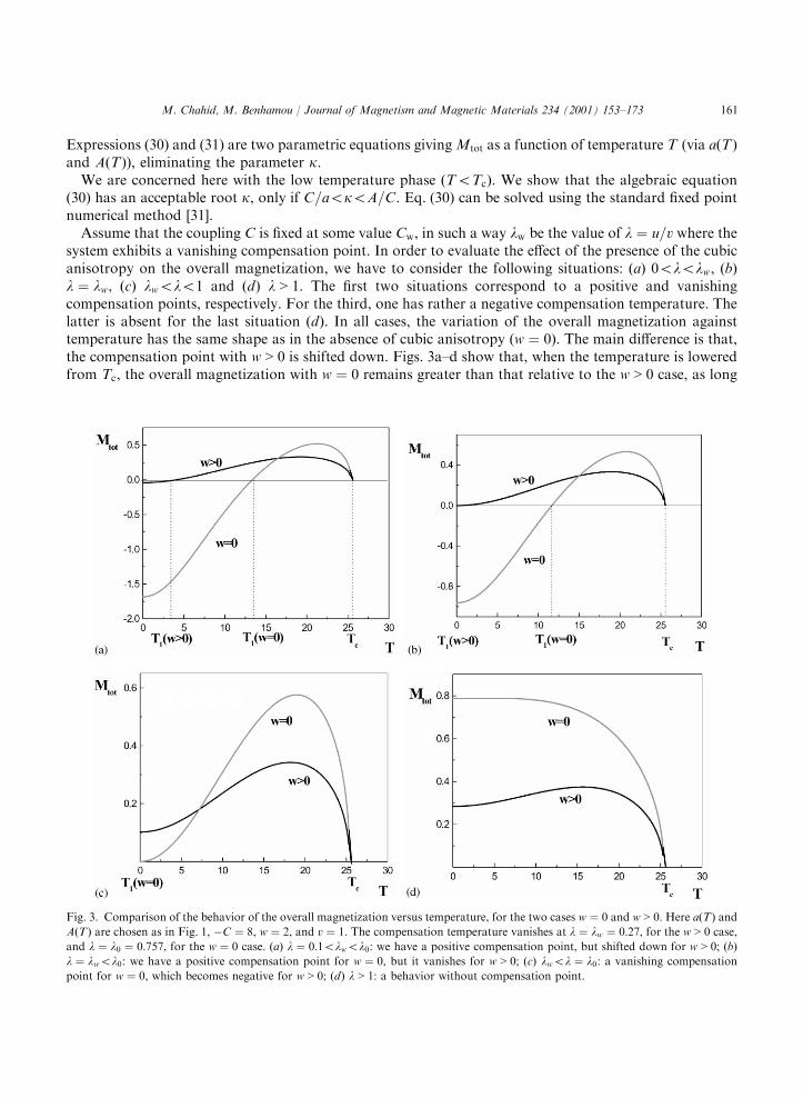
Expressions (30) and (31) are two parametric equations givingMtot as a function of temperature T (via aðTÞand AðTÞ), eliminating the parameter k.We are concerned here with the low temperature phase ðT5TcÞ. We show that the algebraic equation

(30) has an acceptable root k, only if C=a5k5A=C. Eq. (30) can be solved using the standard fixed pointnumerical method [31].Assume that the coupling C is fixed at some value Cw, in such a way lw be the value of l ¼ u=v where the

system exhibits a vanishing compensation point. In order to evaluate the effect of the presence of the cubicanisotropy on the overall magnetization, we have to consider the following situations: ðaÞ 05l5lw, ðbÞl ¼ lw, ðcÞ lw5l51 and ðdÞ l > 1. The first two situations correspond to a positive and vanishingcompensation points, respectively. For the third, one has rather a negative compensation temperature. Thelatter is absent for the last situation ðdÞ. In all cases, the variation of the overall magnetization againsttemperature has the same shape as in the absence of cubic anisotropy ðw ¼ 0Þ. The main difference is that,the compensation point with w > 0 is shifted down. Figs. 3a–d show that, when the temperature is loweredfrom Tc, the overall magnetization with w ¼ 0 remains greater than that relative to the w > 0 case, as long

Fig. 3. Comparison of the behavior of the overall magnetization versus temperature, for the two cases w ¼ 0 and w > 0. Here aðTÞ andAðTÞ are chosen as in Fig. 1, �C ¼ 8, w ¼ 2, and v ¼ 1. The compensation temperature vanishes at l ¼ lw ¼ 0:27, for the w > 0 case,and l ¼ l0 ¼ 0:757, for the w ¼ 0 case. ðaÞ l ¼ 0:15lw5l0: we have a positive compensation point, but shifted down for w > 0; ðbÞl ¼ lw5l0: we have a positive compensation point for w ¼ 0, but it vanishes for w > 0; ðcÞ lw5l ¼ l0: a vanishing compensationpoint for w ¼ 0, which becomes negative for w > 0; ðdÞ l > 1: a behavior without compensation point.


as one is at the right of some characteristic temperature above the compensation point with w ¼ 0. Indeed,this is due to the fact that the coupling C is lowered by the presence of the dipole–dipole interaction. Belowthis temperature, this tendency is inverted. This is consistent with the fact that the overall magnetizationwith w ¼ 0 vanishes before that relative to the w > 0 case.Now, it remains for us to investigate the Arrott-phase-diagram shape.

6. Arrott phase-diagram

The purpose is a quantitative study of the effect of the biquadratic exchange interaction on the shape ofthe Arrott phase-diagram in the ðH=Mtot;M2

totÞ plane. The latter is one of the more convenient ways toinvestigate the overall magnetizationMtot versus an applied magnetic field H. In the case where w ¼ 0, onehas shown [17] the existence of some characteristic temperature T0 below the critical temperature Tc, whichis defined by the equality C ¼ �aðT0Þ. This temperature delimits the region of high coupling constant C. Inaddition, below T0, there is a strong competition between the coupling C and the external magnetic field H.The corresponding curves shape resembles the letter S. Above T0, the behavior is controlled by themagnetic field. The case T ¼ T0 defines a transition regime, where the ferrimagnetic state abruptlydisappears.Now, using the same techniques as in Ref. [17], we find from the state equation (7), (8) that the variables

M2tot and H=Mtot can be given by the following parametric form

H

Mtot¼

uðAþ CÞð1� ZÞ4 � vðaþ CÞZ4 þ vaZ3 � uAð1� ZÞ3 � w að1� ZÞ2 � AZ2� �

ð1� ZÞZ� �

vZ3 � uð1� ZÞ3 þ wZð1� ZÞð1� 2ZÞ; ð32Þ

M2tot ¼

ðaþ CÞð1� ZÞ � ðAþ CÞZ

vZ3 � uð1� ZÞ3 þ wZð1� ZÞð1� 2ZÞ; ð33Þ

which generalizes that relative to the w ¼ 0 case [17]. There, Z ¼ M=Mtot that represents the magneticmoment fraction of the sublattice ðMÞ, stands for the (natural) curve parameter. Obviously, elimination ofthe parameter Z between equations (32) and (33) yields the expected relationship betweenM2

tot and H=Mtot

variables. The above parametric form contains all information about the shape of the Arrott diagram.Now, the aim is to analyze the Arrot-phase-diagram is space of parameter T , C, u, v and w. More

precisely, we will be interested in the influence of the presence of the extra coupling w on the Arrot diagramshape. To this end, as in Refs. [17,18], the starting point is the equation: H=Mtot ¼ �C, where one of itssolutions corresponds to the intermediate configuration of the magnetic moments, which ism0 ¼ 0; M0 6¼ 0ð Þ. According to the parametric form (32), (33), equality H=Mtot ¼ �C yields a fourth-degree algebraic equation satisfied by the parameter Z. The existence of its real solutions depends, of course,on the values of parameters T , C and w. This allows us to distinguish three families of curves following thevalues of w:(i) Weak coupling w: This is characterized by the Arrott diagram shape that resembles the letter S. We

show that, in this regime, the coupling constant w must satisfy the following condition

w5min vaþ C

Aþ C; u

Aþ C

aþ C

�: ð34Þ

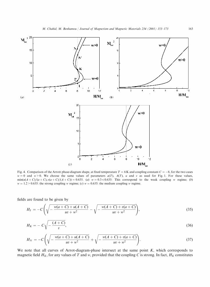
We superpose in Fig. 4a two curves corresponding to the w ¼ 0 and w > 0 cases, respectively, for fixedtemperature T and coupling C, with �C > aðTÞ. These curves show clearly that the presence of w reducesconsiderably the competition between the external magnetic field and the coupling C. Thus, the presence ofw has the tendency to destroy the ferrimagnetism of the system. These typical curves intersect the verticalstraight line defined by equation H=Mtot ¼ �C at three points I , K, and N. The corresponding magnetic


fields are found to be given by

HI ¼ �C

ffiffiffiffiffiffiffiffiffiffiffiffiffiffiffiffiffiffiffiffiffiffiffiffiffiffiffiffiffiffiffiffiffiffiffiffiffiffiffiffiffiffiffiffiffiffiffiffi�wðaþ CÞ þ uðAþ CÞ

uvþ w2

r�

ffiffiffiffiffiffiffiffiffiffiffiffiffiffiffiffiffiffiffiffiffiffiffiffiffiffiffiffiffiffiffiffiffiffiffiffiffiffiffiffiffiffiffiffiffiffiffiffi�wðAþ CÞ þ vðaþ CÞ

uvþ w2

r !; ð35Þ

HK ¼ � C

ffiffiffiffiffiffiffiffiffiffiffiffiffiffiffiffiffiffiffiffiffiffi�

ðAþ CÞv

r; ð36Þ

HN ¼ �C

ffiffiffiffiffiffiffiffiffiffiffiffiffiffiffiffiffiffiffiffiffiffiffiffiffiffiffiffiffiffiffiffiffiffiffiffiffiffiffiffiffiffiffiffiffiffiffiffi�wðaþ CÞ þ uðAþ CÞ

uvþ w2

rþ

ffiffiffiffiffiffiffiffiffiffiffiffiffiffiffiffiffiffiffiffiffiffiffiffiffiffiffiffiffiffiffiffiffiffiffiffiffiffiffiffiffiffiffiffiffiffiffiffi�wðAþ CÞ þ vðaþ CÞ

uvþ w2

r !: ð37Þ

We note that all curves of Arrot-diagram-phase intersect at the same point K , which corresponds tomagnetic fieldHK , for any values of T and w, provided that the coupling C is strong. In fact,HK constitutes

Fig. 4. Comparison of the Arrott phase-diagram shape, at fixed temperature T ¼ 6K and coupling constant C ¼ �8, for the two casesw ¼ 0 and w > 0. We choose the same values of parameters aðTÞ, AðTÞ, u and v as used for Fig. 1. For these values,

minðuðAþ CÞ=ðaþ CÞ; vðaþ CÞ=ðAþCÞÞ ¼ 0:635. ðaÞ w ¼ 0:350:635: This correspond to the weak coupling w regime; ðbÞw ¼ 1:2 > 0:635: the strong coupling w regime; ðcÞ w ¼ 0:635: the medium coupling w regime.


a special magnetic field, and which corresponds to the situation where one of the two moments, say m,vanishes (m0 ¼ 0;M0 6¼ 0). Physically speaking, HK represents the magnetic field beyond which theferrimagnetic state disappears. The configuration m0 ¼ 0;M0 6¼ 0ð Þ is intermediate between the antiparallelmagnetic configuration ðm0 > 0;M050Þ and the parallel one ðm0 > 0;M0 > 0Þ. It is important to note thatthe expression of field HK is not affected by the presence of the biquadratic interaction term wm2M2.However, we show that the magnetic configuration ðm0 ¼ 0;M0 6¼ 0Þ is stable only for small values of thecoupling constant w.A care analysis of expressions (35) and (37) shows that, the magnetic field HI is shifted up, whereas HN is

shifted down in comparison with those relative to the w ¼ 0 case (point I 0 and N 0 in Fig. 4a). This meansthat the region of competition becomes very narrow because of the presence of w (see Fig. 4a).(ii) Strong coupling w: This corresponds to the complete absence of the ferrimagnetic state, and where

the external magnetic field imposes its order. This situation occurs for

w > min vaþ C

Aþ C; u

Aþ C

aþ C

�: ð38Þ

This case is illustrated in Fig. 4b, where we have superposed two curves corresponding to situations withand without coupling constant w. We can see clearly the absence of the behavior that resembles the letter Sof the Arrott phase-diagram shape, for the w > 0 case.(iii) Medium coupling w: This defines a special temperature Tw depending on both C and w and leading

to some special curve. This temperature is found to be given by

w ¼ min vaðTwÞ þ C

AðTwÞ þ C; u

AðTwÞ þ C

aðTwÞ þ C

�: ð39Þ

Of course, Tw is smaller than T0 ðTw5T0Þ, which is its value at w ¼ 0. Above Tw, there is a region where thesystem loses its ferrimagnetic state. Below, one has a temperature regime with a region of competition. Inthis regime, we draw in Fig. 4c two curves relative to w > 0 and w ¼ 0. Remark that the curve with w ¼ 0resembles the letter S, whereas that with w > 0 does not.This completes the static study.The next step shows how kinetics of the para-ferrimagnetic transition can be affected by the presence of a

cubic anisotropy.

7. Kinetics study

A quantitative study of the spin relaxation time of the system was extensively accomplished in our recentwork [19], in the absence of the cubic anisotropy ðw ¼ 0Þ. In particular, we have shown ½19� that dynamicsof the system is governed by two kinds of relaxation times t1 and t2. We found that these times areassociated with short and long wavelength fluctuations, respectively. The purpose, here, is to evaluate theeffect of the biquadratic exchange interaction on kinetics. The material is assumed to be in an equilibriumstate at an initial temperature Ti far from the critical point Tc. Suppose that this temperature is changed toa final value Tf very close to Tc. In the temperature interval Ti5T5Tf , both order parameters mðtÞ andMðtÞ vary with time t, from their initial values mi andMi to final ones mf andMf . We are interested in howthe order parameters ðm;MÞ relax to final equilibrium state mf ;Mf

� �.

To investigate kinetics, we assume that the time-dependent order parameters solve the Langevinequations (without noise) [32,33]

dm

dt¼ �r

dFdm

;dM

dt¼ �r

dFdM

; ð40Þ


where r is some positive constant and F is the free energy, relations (1) and (2). In fact, quantities of interestare rather the shifts of these order parameters from their mean values %mm and %MM, i.e.

m ¼ %mmþ dm; M ¼ %MM þ dM: ð41Þ

Within the framework of the linearized theory and by expanding to first order the free energy F ofexpression (1), (2) (with H ¼ 0) around the static configuration ð %mm; %MMÞ, we find that the order parametersshifts dm; dMð Þ satisfy the linear coupled equations

ddmdt

ddMdt

" #¼ �r

%aa %CC

%CC %AA

" #%mm; %MM

dm

dM

" #: ð42Þ

We have used the short notations

%aa ¼ aþ 3u %mm2 þ w %MM2; ð43Þ

%AA ¼ Aþ 3v %MM2þ w %mm2; ð44Þ

%CC ¼ �C þ 2w %mm %MM: ð45Þ

The static order parameters %mm and %MM solve the state equation (7), (8).The linear differential system (42) can be solved using the standard method based on the matrix

diagonalization. We give simply the result

dMtot ¼ dmþ dM ¼ H e�t=t1 þ G e�t=t2 ; ð46Þ

where dMtot denotes the fluctuation of the overall magnetization. There, H and G are known amplitudes.We find that the relaxation times t1 and t2 read

t�11 ¼r2

%aaþ %AA�ffiffiffiffiffiffiffiffiffiffiffiffiffiffiffiffiffiffiffiffiffiffiffiffiffiffiffiffiffiffiffið %aa� %AAÞ2 þ 4 %CC

2q� �

; ð47Þ

t�12 ¼r2

%aaþ %AAþffiffiffiffiffiffiffiffiffiffiffiffiffiffiffiffiffiffiffiffiffiffiffiffiffiffiffiffiffiffiffið %aa� %AAÞ2 þ 4 %CC

2q� �

: ð48Þ

Recall that the appearance of these two relaxation times is in good agreement with some results reported ina recent experiment [11] on the Curie–Weiss paramagnet compound LixNi2�xO2, where the composition xis close to 1. As in the w ¼ 0 case, t2 is a small time that governs local dynamics. This latter can beinterpreted as the necessary time to build-up microdomains of spins of antiparallel alignment. The longestrelaxation time t1 is relevant for physics, since it drives the material to undergo a phase transition. In fact,t1 is the necessary time to establish a ferrimagnetic order, and then, it controls long-scale dynamics. A careanalysis of expression (47) shows that t1 increases with increasing dipole–dipole coupling w. This tendencyis illustrated in Fig. 5, which shows the variation of the relaxation time t1 versus w, at fixed C and T . Thevariation of t1 versus T , at fixed C and w > 0, is depicted in Fig. 6. This latter calls some comments. First, t1diverges, of course, at Tc, but with a different amplitude depending on whether one is above or below thecritical point. It is important to note that the presence of the biquadratic exchange interaction does notaffect the behavior of t1 in the high temperature regime. At a fixed temperature near but below Tc, therelaxation time with w > 0 is greater than that with w ¼ 0. This is due to the fact that the presence of w isunfavorable to the growth of macrodomains of antiparallel spins. Thus, the system with a cubic anisotropyinteraction relaxes more slowly. Below some temperature, depending on both C and w, this situation isinverted. This has as origin, the fact that when the ordered state of the system, with w ¼ 0, is reached, thislatter has tendency to be more stable. While the relaxation of the system with a dipole–dipole interaction


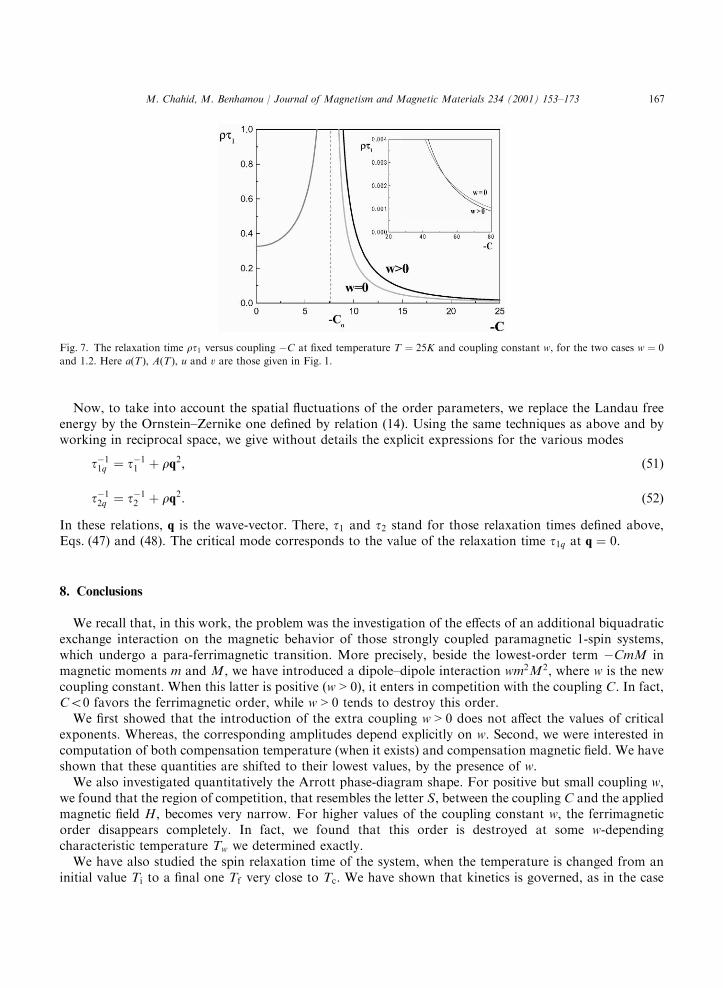
(w > 0) is accelerated near the compensation point. This is clearly shown in Fig. 4a, for instance. The sameconclusion remains valid for the variation of t1 versus C, at fixed T and w, which is depicted in Fig. 7.Near Tc and from its general expression, the relaxation time t1 scales as

t1 tj j�y; ð49Þ

where t ¼ ðT � TcÞ=Tc is the reduced temperature. There, y ¼ 1 is a dynamic exponent. In terms ofcorrelation length x tj j�n, the above scaling law rewrites

t1 xz; ð50Þ

with the dynamic exponent z ¼ n=y ¼ 2. These scaling laws, which take the same form as those relative tothe w ¼ 0 case, show that the longest relaxation time diverges as the critical temperature is reached. Theonly difference is that, the known corresponding amplitudes we ignored depend on the extra coupling w.

Fig. 5. The relaxation time rt1 versus the coupling constant w, at fixed coupling C ¼ �8 and temperature T ¼ 25K. Here a ðTÞ andAðTÞ are chosen as in Fig. 1, u ¼ 3 and v ¼ 1.

Fig. 6. The relaxation time rt1 versus temperature, at fixed coupling constants C and w, for the two cases w ¼ 0 and w ¼ 1:2. HereaðTÞ, AðTÞ, u and v are those of Fig. 1, and C ¼ �8; Tc ¼ 25:4K.


Now, to take into account the spatial fluctuations of the order parameters, we replace the Landau freeenergy by the Ornstein–Zernike one defined by relation (14). Using the same techniques as above and byworking in reciprocal space, we give without details the explicit expressions for the various modes

t�11q ¼ t�11 þ rq2; ð51Þ

t�12q ¼ t�12 þ rq2: ð52Þ

In these relations, q is the wave-vector. There, t1 and t2 stand for those relaxation times defined above,Eqs. (47) and (48). The critical mode corresponds to the value of the relaxation time t1q at q ¼ 0.

8. Conclusions

We recall that, in this work, the problem was the investigation of the effects of an additional biquadraticexchange interaction on the magnetic behavior of those strongly coupled paramagnetic 1-spin systems,which undergo a para-ferrimagnetic transition. More precisely, beside the lowest-order term �CmM inmagnetic moments m and M, we have introduced a dipole–dipole interaction wm2M2, where w is the newcoupling constant. When this latter is positive ðw > 0Þ, it enters in competition with the coupling C. In fact,C50 favors the ferrimagnetic order, while w > 0 tends to destroy this order.We first showed that the introduction of the extra coupling w > 0 does not affect the values of critical

exponents. Whereas, the corresponding amplitudes depend explicitly on w. Second, we were interested incomputation of both compensation temperature (when it exists) and compensation magnetic field. We haveshown that these quantities are shifted to their lowest values, by the presence of w.We also investigated quantitatively the Arrott phase-diagram shape. For positive but small coupling w,

we found that the region of competition, that resembles the letter S, between the coupling C and the appliedmagnetic field H, becomes very narrow. For higher values of the coupling constant w, the ferrimagneticorder disappears completely. In fact, we found that this order is destroyed at some w-dependingcharacteristic temperature Tw we determined exactly.We have also studied the spin relaxation time of the system, when the temperature is changed from an

initial value Ti to a final one Tf very close to Tc. We have shown that kinetics is governed, as in the case

Fig. 7. The relaxation time rt1 versus coupling �C at fixed temperature T ¼ 25K and coupling constant w, for the two cases w ¼ 0

and 1.2. Here aðTÞ, AðTÞ, u and v are those given in Fig. 1.


where w ¼ 0, by two kinds of relaxation times t1 and t2. The former, which is associated with long-wavelength fluctuations, is a long time and the relevant one, since it drives the system to undergo a phasetransition. The second is a short time, and which controls local dynamics. In comparison with the w ¼ 0case, we found that, near Tc, the relaxation time t1 with w > 0 increases more rapidly. Spacial variations ofrelaxation time were also taken into account, and we have shown that the critical mode corresponds to thezero scattering-angle limit, i.e. q ! 0.It is important to note that the existence of two relaxation times was experimentally confirmed by

Reimers and co-workers [11], on the 1/2-spin Curie–Weiss paramagnetic compound LixNi2�xO2, where thecomposition x is very close to 1. The authors have shown that the relaxation time of the magnetization,when the magnetic field is lowered from 0:05 to 0:01T, keeping the temperature fixed, occurs on more thanone time scale. Futures experiments on 1-spin compounds would be desirable, and in principle, one shouldobserve two relaxation times as predicted by our theoretical approach.Finally, we note that the mean-field treatement used here, is valid, only, as long as one is above the upper

critical dimension dc ¼ 4. Below, it will be interesting to examine the problem within the framework ofRenormalization-Group, in order to get a more realistic critical behavior of the system. Such a work is inprogress [25].

Acknowledgements

We would like to thank our referee for his pertinent suggestions.

Appendix

The purpose of this appendix is to show how the continuous model of free energy (1), (2) for 1-spinsystems, with biquadratic exchange interaction, can emerge from a discrete 1-spin Hamiltonian. To thisend, use will be made of the so-called Blume–Emery–Griffiths model [34], written for the case of twostrongly coupled Curie–Weiss paramagnetic subsystems exhibiting a para-ferrimagnetic transition.Consider two coupled sublattices O1 and O2 of Euclidean dimension d. On each site i 2 O1 and i0 2 O2,we attribute two variables Si ¼ �1; 0;þ1 and Si0 ¼ �1; 0;þ1, respectively. We denote by J1 and J2 theexchange integrals inside O1 and O2. We denote by J12 and #JJ12 the polar and the quadripolar interactionsbetween O1 and O2, respectively. To a given configuration of spins, we associate the discrete Hamiltonian

IH ¼ �Xij

½J1�ijSiSj �Xi0j0

½J2�i0j0Si0Sj0 �Xij0

½J12�ij0SiSj0 �Xij

#JJ12� �

ij0S2i S

2j0 �

Xi

hiSi

�Xi0

hi0Si0 �Xi

DiS2i �

Xi0

Di0S2i0 : ðA:1Þ

We have ½J1�ij ¼ J1, ½J2�i0j0 ¼ J2, ½ #JJ12�ij0 ¼ #JJ12 and #JJ12� �

ij0¼ #JJ12, for nearest neighbors sites, and 0, otherwise.

We will suppose that J1 > 0 and J2 > 0 (ferromagnetic couplings), #JJ1250 (antiferromagnetic coupling) and#JJ1250. The variables ha and Da a ¼ i; i0ð Þ stand, respectively, for the direct and the crystal fields applied tosites i 2 O1 and i0 2 O2.The starting point is the partition function or the generating functional that is given as usual by

Z *hh; *DD� �

¼X

*SSi¼0;�1f gexp �bIHf g ¼

X*SSi¼0;�1f g

expXij

Kij*SSi*SSj þ

Xij

#KKij*SS2

i*SS2

j þXi

*hhi *SSi þXi

*DDi*SS2

i

( ):

ðA:2Þ


Here, b ¼ kBTð Þ�1, where T is the absolute temperature and kB is the Boltzmann constant. Summation inEq. (A.2) is performed over all 3 O1j j � 3 O2j j possible configurations, where Oaj j denotes the number of sitesinside the sublattice a. We have redefined the exchange integrals to get dimensionless ones, according to

Kij ¼

b J1½ �ij ; ði; jÞ 2 O1 � O1;

b J2½ �i0j0 ; ði0; j0Þ 2 O2 � O2;

b J12½ �ij0 ; ði; j0Þ 2 O1 � O2

8><>: ðA:3Þ

and

#KKij ¼b #JJ12� �

ij0; ði; j0Þ 2 O1 � O2;

0; otherwise:

(ðA:4Þ

We have used the notations

*SSi ¼Si; i 2 O1;

Si0 ; i0 2 O2;

(ðA:5Þ

*hhi ¼bhi; i 2 O1;

bhi0 ; i0 2 O2;

(ðA:6Þ

*DDi ¼bDi; i 2 O1;

bDi0 ; i0 2 O2:

(ðA:7Þ

Thus, *hhi and *DDi are dimensionless fields.Now, the passage from discrete to continuous formulation can be made through the standard Gaussian

integral representationZ þ1

�1

YNi¼1

dxi exp �1

4

Xij

xiDijxj þXi

Sixi

!¼ const� exp

Xij

SiD�1ij Sj

!; ðA:8Þ

where D ¼ Dij

� �is any positive definite symmetric squared matrix. In our case, we will use a double

Gaussian transformation, and D is either the inverse of the coupling constant matrix K or the inverse of #KKdefined above. Thanks to this representation and performing summation over the spin variables, thepartition function defined by expression (A.2) can be rewritten as a functional integral

Z *hh; *DD� �

¼Z0o �

Z þ1

�1

Yi2O

dfi dsi

" #exp �

1

4

Xij

ðfi � *hhiÞ K�1� �ijfj � *hhj� �( )

� exp �1

4

Xij

si � *DDi

� �#KK�1

h iijsj � *DDj

� �( )exp

Xi

A fi;si� � !

; ðA:9Þ

where Z0o is a normalization constant, and O ¼ O1 [ O2. There,

A fi;si� �

¼ ln 1þ 2esicosh fi

� �: ðA:10Þ

The fields fi and si are defined by

fi ¼ji; i 2 O1;

ci0 ; i0 2 O2

(ðA:11Þ


and

si ¼j2i ; i 2 O1;

c2i0 ; i0 2 O2:

(ðA:12Þ

The integral (A.9) can be calculated using the steepest descent method [35], which gives, at lowest order,the mean-field theory. We first perform the translations

fi ¼ Xi þ *ffi ðA:13Þ

and

si ¼ Yi þ *ssi; ðA:14Þ

where Xi and Yi are the configurations giving the lowest potential energy. There, *ffi and *ssi are thefluctuations around the saddle point (classical solutions). The method consists in making expansion inpowers of *ffi and *ssi. We then get

�bIH½f;s� ¼ �bIH½X ;Y � �1

4*ffK�1 *ffþ

1

2

Xi

*ff2

i

q2AqX2

i

�1

4*ss #KK

�1*ssþ

1

2

Xi

*ss2iq2AqY2

i

þ . . . : ðA:15Þ

With these considerations, the generating functional becomes

Z *hh; *DD� �

¼ const:eWo*hh; *DD½ � �

Z þ1

�1

Yi2O

d *ffi

" #� exp �

1

4

Xij

*ffi½K�1�ij *ffj þ

1

2

Xi

*ff2

i A00ðXiÞ þ � � �

( )

�Z þ1

�1

Yi2O

d *ssi

" #� exp �

1

4

Xij

*ssi #KK�1

h iij*ssj þ

1

2

Xi

*ss2i A00ðYiÞ þ � � �

( ): ðA:16Þ

The first approximation to the Helmoltz free energy W *hh; *DD� �

¼ lnZ *hh; *DD� �

is Wo*hh; *DD� �

, such as

Wo*hh; *DD� �

¼ �1

4

Xij

Xi � *hhi� �

K�1� �ijXj � *hhj� �

�1

4

Xij

Yi � *DDi

� �#KK�1

h iijYj � *DDj

� �

þXi

AðXi;YiÞ

Xi¼Xi ½ *hh�; Yi¼Yi

*DD½ �: ðA:17Þ

Now, consider the order parameters *mmi and *qqi relative to a site i of the lattice O ¼ O1 [ O2, and denote

*mmi ¼mi; i 2 O1;

Mi0 ; i0 2 O2;

(ðA:18Þ

*qqi ¼m2i ; i 2 O1;

M2i0 ; i0 2 O2;

(ðA:19Þ

which are given by the first functional derivative of the free energy, with respect to fields *hhi and *DDi

*mmi ¼dW *hh; *DD

� �d *hhi

; *qqi ¼dW *hh; *DD

� �d *DDi

: ðA:20Þ


To lowest order, we have

*mmi ¼qAðXi;YiÞ

qXi

¼1

2

Xij

K�1� �ijXj � *hhj� �

; ðA:21Þ

*qqi ¼qAðXi;YiÞ

qYi

¼1

2

Xij

#KK�1

h iijYj � *DDj

� �: ðA:22Þ

It will be convenient to discuss the problem in terms of order parameters *mm and *qq. The correspondingthermodynamic potential or proper generating functional Go *mm; *qq½ � is the Legendre transform of theHelmoltz free energy, i.e.

Go *mm; *qq½ � þWo½ *mm; *qq� ¼Xi2O

*hhi *mmi þXi2O

*DDi *qqi; ðA:23Þ

in which *hhi’s and *DDi’s solve equations (A.21) and (A.22). This yields the tree approximation expression ofthe thermodynamic potential

Go *mm; *qq½ � ¼ �Xij

*mmiKij *mmj �Xij

*qqi #KKij *qqj þXi

Bð *mmi; *qqiÞ; ðA:24Þ

with

Bð *mmi; *qqiÞ ¼ Xi *mmi þ Yi *qqi � A Xi;Yið Þ� �

*mmi ¼qAqXi

; *qqi ¼qAqYi

: ðA:25Þ

More explicitly, for the considered model, we obtain

Bð *mmi; *qqiÞ ¼*mmi � *qqi2

�ln

*qqi þ *mmi

*qqi � *mmi

�þ *qqiln

*qqi þ *mmi

2 1� *qqi� �

!þ lnð1� *qqiÞ: ðA:26Þ

In the case of uniform direct and crystal fields, that is for *hhi ¼ *hh ¼ H and *DDi ¼ D, the order parametersare independent on sites, and we may write

*mm ¼m; i 2 O1;

M; i 2 O2;

(ðA:27Þ

*qq ¼m2; i 2 O1

M2; i 2 O2:

(ðA:28Þ

In the high temperature phase (paramagnetic), the three spin-states �1, 0 and þ1 are equiprobable. Weshow, within this temperature- range, that the order parameters *mm and *qq are given by

*mm ¼ Sh i ¼ 0; ðA:29Þ

*qq ¼ S2 !

¼2

3: ðA:30Þ

Equality (A.30) shows that the true order parameter is not *qq but rather

*QQ ¼ *qq�2

3: ðA:31Þ


The expression (A.26) then becomes

Bð *mm; *qqÞ ¼*mm� *QQ� 2

3

2

!ln

1þ 32

*QQþ *mm� �

1þ 32

*QQ� *mm� �

!þ *QQþ

2

3

�ln

1þ 32

*QQþ *mm� �

1� 3 *QQ

!þ ln

1

3� *QQ

�: ðA:32Þ

The last step consists in performing expansion of logarithmic function around the critical point, whereboth order parameters *mm and *QQ are small. Thus, Eqs. (A.25)–(A.32) yield the desired free energyF ½m;M� ¼ kBT Go m;M½ � �HðmþMÞ � Dðm2 þM2Þ

" #. Explicitly, we have

F ½m;M� ¼a

2m2 þ

A

2M2 þ

u

4m4 þ

v

4M4 � CmM

þw

2m2M2 �HðmþMÞ þ � � � ; ðA:33Þ

with

a ¼ �3

2� 2D�

J1z1kBT

; A ¼ �3

2� 2D�

J2z2kBT

; u ¼ v ¼45

8ðA:34Þ

and

C ¼J12z12kBT

50; w ¼ �2 #JJ12z12kBT

> 0: ðA:35Þ

Here, z1, z2 and z12 are, respectively, the numbers of nearest neighbors inside the sublattices O1 and O2, andbetween O1 and O2.The free energy (A.33) defines the Landau continuous model used in this work, to describe the super-

weak ferrimagnetism arising from 1-spin systems.

References

[1] K.U. Neumann, J. Crangle, K.R.A. Ziebeck, J. Magn. Magn. Mater. 127 (1993) 47.

[2] G. Chouteau, R. Yazami, Private Communication.

[3] M.G.S.R. Thomas, W.I.F. David, J.B. Goodenough, P.G. Groves, Mater. Res. Bull. 20 (1985) 1137.

[4] J.R. Dahn, V. Von Sacken, M.W. Juzkow, H. Al Janaby, J. Electrochem. Soc. 138 (1991) 2207.

[5] T. Ohzuku, A. Ueda, M. Nagayama, J. Electrochem. Soc. 140 (1993) 1862.

[6] C. Delmas, C. Fouassier, P. Hagenmuller, Mater. Sci. Eng. 31 (1977) 297.

[7] W. Pauli, Z. Physik 41 (1927) 81.

[8] C. Kittel, Physique de l’Etat Solide, Dunod and Bordas, Paris, 1983.

[9] G. Dutta, A. Manthiram, J.B. Goodenough, J.C. Grenier, J. Solid State Chem. 81 (1989) 203.

[10] A. Rougier, Th"eese d’Universit!ee, Bordeaux, France, 1995.

[11] J.N. Reimers, J.R. Dahn, J.E. Greedan, C.V. Starger, G. Liu, I. Davidson, U. Von Sacken, J. Solid State Chem. 102 (1993) 542.

[12] K. Hirakawa, R. Osborn, A.D. Taylor, K. Tadeka, J. Phys. Soc. Japan 59 (1990) 3081.

[13] J.C. Tol!eedano, The Landau Theory of Phase Transition, World Scientific, Singapore, 1987.

[14] H.E. Stanley, Introduction to Phase Transitions and Critical Phenomena, (Clarendron Press, Oxford, 1971).

[15] D. Amit, Field Theory, The Renormalization Group and Critical Phenomena, McGraw-Hill, New York, 1978.

[16] K.U. Neumann, Lipinski, K.R.A. Ziebeck, Solid State Commun 91 (1994) 443.

[17] B. El Houari, M. Benhamou, M. El Hafidi, G. Chouteau, J. Magn. Magn. Mater. 166 (1997) 97.

[18] B. El Houari, M. Benhamou, J. Magn. Magn. Mater. 172 (1997) 259.

[19] M. Chahid, M. Benhamou, J. Magn. Magn. Mater. 218 (2000) 287.

[20] M. Chahid, M. Benhamou, J. Magn. Magn. Mater. 213 (2000) 219.

[21] J.C. Collins, Renormalization, Cambridge University Press, Cambridge, 1985.

[22] J. Zinn-Justin, Quantum Field Theory and Critical Phenomena, Clarendon Press, Oxford, 1989.

[23] C. Itzykson, J.M. Drouffe, Statistical Field Theory: 1 and 2, Cambridge University Press, Cambridge, 1989.

[24] J.B. Goodenough, D.G. Wickham, W.J. Croft, J. Phys. Chem. Solid 51 (1958) 07.

[25] M. Benhamou, M. Chahid, in preparation.


[26] P. Weiss, R. Forrer, Ann. Phys. Paris 5 (1926) 153.

[27] C. Chahine, Thermodynamique Statistique, Dunod and Bordas, Paris, 1986.

[28] L. N!eeel, Ann. Phys. Paris 3 (1948) 137.

[29] D.H. Martin, Magnetism in Solids, Illife Books LTD, London, 1967.

[30] A. Herpin, Th!eeorie du Magn!eetisme, Press Universitaire de France, Paris, 1968.

[31] R.L. Burden, J.D. Faires, J. Douglas, Numerical Analysis, PWS Publisher, Boston, 1981.

[32] L.D Landau, E.M. Lifshitz, M!eecanique Statistique, Chapter XIV, Edition Mir, Moscou.

[33] S.K. Ma, Modern Theory of Critical Phenomena, Benjamin Cummins, Menlo Park, CA, 1976.

[34] F.Y. Wu, Chinese J. Phys. 30 (1992) 157.

[35] E. Br!eezin, J.C. Le Guillou, J. Zinn-Justin, in: C. Domb, M.S. Green (Eds.), Phase Transition and Critical Phenomena, Vol. 6,

Academic Press, New York, 1976.


paramagnetic–ferrimagnetic transition in strong coupling paramagnetic systems: effect of cubic...

Documents