parallel in-memory evaluation of spatial joins

Parallel In-Memory Evaluation of Spatial JoinsDimitrios Tsitsigkos

Information Management Systems InstituteAthena RC, Athens, Greece

[email protected]

Panagiotis BourosInstitute of Computer Science

Johannes Gutenberg University Mainz, [email protected]

Nikos MamoulisDepartment of Computer Science and Engineering

University of Ioannina, [email protected]

Manolis TerrovitisInformation Management Systems Institute

Athena RC, Athens, [email protected]

ABSTRACTWe study the in-memory and parallel evaluation of spatial joins,by tuning a classic partitioning based algorithm. Our study showsthat, compared to a straightforward implementation of the algo-rithm, performance can be improved signi�cantly. We also showhow to select appropriate partitioning parameters based on datastatistics, in order to tune the algorithm for the given join inputs.Our parallel implementation scales gracefully with the number ofthreads reducing the cost of the join to at most one second evenfor join inputs with tens of millions of rectangles.

CCS CONCEPTS• Information systems→ Join algorithms; Spatial-temporalsystems; Parallel and distributed DBMSs;

KEYWORDSSpatial Join, In-memory Data Management, Parallel Processing

ACM Reference Format:Dimitrios Tsitsigkos, Panagiotis Bouros, Nikos Mamoulis, and Manolis Ter-rovitis. 2019. Parallel In-Memory Evaluation of Spatial Joins. In 27th ACMSIGSPATIAL International Conference on Advances in Geographic InformationSystems (SIGSPATIAL ’19), November 5–8, 2019, Chicago, IL, USA. ACM, NewYork, NY, USA, 4 pages. https://doi.org/10.1145/3347146.3359343

1 INTRODUCTIONThe spatial join is a well-studied fundamental operation. Given twocollections of spatial objects R and S , the spatial intersection joinreturns all (r , s) pairs, such that r 2 R, s 2 S and r and s have at leastone common point. Due to the potentially complex geometry ofthe objects, intersection joins are typically processed in two steps.The �lter step applies on spatial approximations of the objects,typically their minimum bounding rectangle (MBR). For each pairof object MBRs that intersect, the object geometries are fetched

Permission to make digital or hard copies of all or part of this work for personal orclassroom use is granted without fee provided that copies are not made or distributedfor pro�t or commercial advantage and that copies bear this notice and the full citationon the �rst page. Copyrights for components of this work owned by others than ACMmust be honored. Abstracting with credit is permitted. To copy otherwise, or republish,to post on servers or to redistribute to lists, requires prior speci�c permission and/or afee. Request permissions from [email protected] ’19, November 5–8, 2019, Chicago, IL, USA© 2019 Association for Computing Machinery.ACM ISBN 978-1-4503-6909-1/19/11. . . $15.00https://doi.org/10.1145/3347146.3359343

and compared in a re�nement step. Similar to the vast majority ofprevious work [7], we focus on the �lter step.

A wide range of spatial join algorithms have been proposed inthe literature [3]. Given the fact that main memory chips becomebigger and faster, in-memory join processing has recently receiveda lot of attendance [8]. In addition, given that commodity hardwaresupports parallel processing, multi-core join evaluation has alsobeen the focus of recent research. Hence, in this paper, we target theparallel in-memory evaluation of spatial joins on modern hardware.

Our focus is the optimization of the simple, but powerful parti-tioning-based spatial join (PBSM) algorithm [9]. PBSM is shown toperform well in previous studies [8] and used by most distributedspatial data management systems [1, 6, 11]. In a nutshell, bothdatasets are �rst partitioned using a regular grid; each tile (cell)of the grid gets all rectangles that intersect it. Each tile de�nes asmaller spatial join task. These tasks are independent and can be ex-ecuted in parallel, assigned to di�erent threads or even to di�erentmachines in distributed evaluation. Typically a plane sweep algo-rithm based on forward scans [4] is used to process each task. Forexample, consider the two sets of MBRs of Figure 1a. Partitioningthe rectangles using a 3 ⇥ 3 grid creates 9 independent spatial jointasks, one for each tile. Note that some rectangles may be replicatedto multiple tiles. Because of this, some pairs of rectangles may befound to intersect in multiple tiles; e.g., r1 intersects s1 in tiles (0,0)and (0,1). Duplicate join results can be avoided by reporting a pairof rectangles only if a pre-determined reference point (typically,the top-left corner) of the intersection region is in the tile [5]; e.g.,(r1, s1) is only reported by tile (0,0).

Currently, there is no comprehensive study so far on how thenumber and type of partitions should be de�ned. In this paper, weevaluate a 1D partitioning that divides the space into stripes (seeFigure 1b), as opposed to the classic 2D partitioning, which uses agrid. Further, we investigate, for each partition, the best direction ofthe sweep line. Finally, we show how both the partitioning and the

r1 r2

r3r4 r5

r6 r7

s1s2

s3s4

s5 s6

0

1

2

0 1 2r1 r2

r3r4 r5

r6 r7

s1s2

s3s4

s5 s6

0 1 2 3

r1 r2

r3r4 r5

r6 r7

s1s2

s3s4

s5 s6

0

1

2

0 1 2r1 r2

r3r4 r5

r6 r7

s1s2

s3s4

s5 s6

0 1 2 3

Figure 1: Example of PBSM: (a) 2D and (b) 1D partitioning

https://doi.org/10.1145/3347146.3359343

https://doi.org/10.1145/3347146.3359343

SIGSPATIAL ’19, November 5–8, 2019, Chicago, IL, USA D. Tsitsigkos et al.

joining phases of the algorithm can be parallelized. Based on ourtests, the 1D partitioning results in a more e�cient algorithm. Also,increasing the number of partitions improves the performance ofthe algorithm, up to a point where adding more partitions startshaving a negative e�ect. We present a number of empirical rulesdriven from data statistics (globally and locally for each partition)that can guide the selection of the algorithm’s parameters. Finally,we evaluate the performance of the parallel version of the algorithmand show that it scales gracefully with the number of cores.

2 TUNING PBSMPBSM is a popular spatial join algorithm for the following reasons:

• PBSM assumes no preprocessing or indexing of the data, so itcan be applied on dynamically generated spatial data.

• The partitions de�ne independent join tasks that can easily bedistributed and/or parallelized.

• The number of join tasks is the same as the number of partitions.• Producing duplicate results can be easily avoided.• Implementing this approach is fairly easy.• Previous studies [8] have shown that the performance of PBSMcan hardly be beaten by more sophisticated approaches basedon indexing or adaptive partitioning.

In the following, we explore the directions along which we cantune PBSM to improve its performance. We assume that PBSM usesthe plane sweep algorithm of [4] for each partition-partition join.

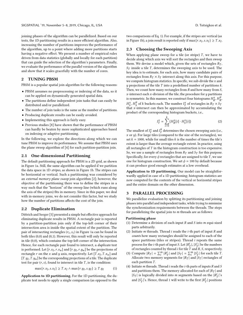
2.1 One-dimensional PartitioningThe default partitioning approach for PBSM is a 2D grid, as shownin Figure 1a. Still, the same algorithm can be applied if we partitionthe data space in 1D stripes, as shown in Figure 1b. The stripes canbe horizontal or vertical. Such a partitioning was considered byan external memory plane sweep join algorithm [2]; however, theobjective of the partitioning there was to de�ne the stripes in away such that the “horizon” of the sweep line (which runs alongthe axis of the stripes) �ts in memory. Since in this paper, we dealwith in-memory joins, we do not consider this factor, but we studyhow the number of partitions a�ects the cost of the join.

2.2 Duplicate EliminationDittrich and Seeger [5] presented a simple but e�ective approach foreliminating duplicate results in PBSM. A rectangle pair is reportedby a partition-partition join only if the top-left corner of theirintersection area is inside the spatial extent of the partition. Thepair of intersecting rectangles (r1, s1) in Figure 1a can be found inboth tiles (0,0) and (0,1). However, this result will only be reportedin tile (0,0), which contains the top-left corner of the intersection.Hence, for each rectangle pair found to intersect, a duplicate testis performed. Let [r .xl , r .xu ] and [r .�l , r .�u ] be the projections ofrectangle r on the x and � axis, respectively. Let [T .xl ,T .xu ] and[T .�l ,T .�u ] be the corresponding projections of a tile. The duplicatetest for pair (r , s), found to intersect in tile T , is the condition:

max{r .xl , s .xl } � T .xl ^max{r .�l , s .�l } � T .�l (1)

Application to 1D partitioning. For the 1D partitioning, the du-plicate test needs to apply a single comparison (as opposed to the

two comparisons of Eq. 1). For example, if the stripes are vertical (asin Figure 1b), a join result is reported only ifmax{r .xl , s .xl } � T .xl .

2.3 Choosing the Sweeping AxisWhen applying plane sweep for a tile (or stripe) T , we have todecide along which axis we will sort the rectangles and then sweepthem. We devise a model which, given the sets of rectangles RT ,ST inside a tile T , determines the sweeping axis to be used. Thekey idea is to estimate, for each axis, how many candidate pairs ofrectangles from RT ⇥ ST intersect along this axis. For this purpose,we compute histogram statistics. In speci�c, we sub-divide the x and� projections of the tile T into a prede�ned number of partitions k .Then, we count howmany rectangles from R and howmany from S ,x-intersect each x-division of the tile; the procedure for � partitionsis symmetric. In this manner, we construct four histogramsHx

R ,H�R ,

HxS , H

�S of k buckets each. The number IxT of rectangles in RT ⇥ ST

that x-intersect can then be approximated by accumulating theproduct of the corresponding histogram buckets, i.e.,

IxT =k’i=0

{HxR [i] · H

xS [i]} (2)

The smallest of IxT and I�T determines the chosen sweeping axis (i.e.,x or �). For large tiles (compared to the size of the rectangles), weset k = 1000, while for small tiles k is the number of times the tile’sextent is larger than the average rectangle extent. In practice, usingall rectangles of T in the histogram construction is too expensive.So, we use a sample of rectangles from RT and ST for this purpose.Speci�cally, for every � rectangles that are assigned to tileT , we useone for histogram construction. We set � = 100 by default becauseit can produce good enough estimates at a low overhead.

Application to 1D partitioning. Our model can be straightfor-wardly applied in case of a 1D partitioning; histogram statistics arenow computed for the contents of the vertical or horizontal stripesand the entire domain on the other dimension.

3 PARALLEL PROCESSINGWe parallelize evaluation by splitting its partitioning and joiningphases into parallel and independent tasks, while trying tominimizethe synchronization requirements between the threads. The stepsfor parallelizing the spatial join tom threads are as follows:

Partitioning phase(1) Determine a division of each input R and S intom equi-sized

parts arbitrarily.(2) Initiatem threads. Thread i reads the i-th part of input R and

counts how many rectangles should be assigned to each of thespace partitions (tiles or stripes). Thread i repeats the sameprocess for the i-th part of input S . Let |RiT |, |S

iT | be the numbers

of rectangles counted by thread i for tileT and R, S , respectively.(3) Compute |RT | =

Õmi |RiT | and |ST | =

Õmi |SiT | for each tile T .

Allocate two memory segments for |RT | and |ST | rectangles ofeach partition T .

(4) Initiatem threads. Thread i reads the i-th parts of inputs R and Sand partitions them. The memory allocated for each of |RT | and|ST | is logically divided intom segments based on the |RiT |’sand |SiT |’s. Hence, thread 1 will write to the �rst |R1T | positions

Parallel In-Memory Evaluation of Spatial Joins SIGSPATIAL ’19, November 5–8, 2019, Chicago, IL, USA

Table 1: Datasets used in the experimentssource dataset alias cardinality avg. x -extent avg. �-extent

Tiger 2015

AREAWATER T 2 2.3M 0.000007230 0.000022958EDGES T 4 70M 0.000006103 0.00001982

LINEARWATER T 5 5.8M 0.000022243 0.000073195ROADS T 8 20M 0.000012538 0.000040672

OSM

Buildings O3 115M 0.00000056 0.000000782Lakes O5 8.4M 0.000021017 0.000028236Parks O6 10M 0.000016544 0.000022294Roads O9 72M 0.000010549 0.000016281

of |RT |, thread 2 to the next |R2T | positions, etc. After all threadscomplete partitioning, we will have the entire set of rectanglesthat fall in each tile continuously in memory.

Joining phase(5) Construct two sorting tasks for each tile T (one for RT and one

for ST ). Assign the sorting tasks to them threads.(6) Construct a join task for each tileT (one for RT and one for ST ).

Assign the join tasks to them threads.

Step 2 is applied to make proper memory allocation and preventexpensive dynamic allocations. It also facilitates the output of par-allel partitioning for each tileT to be continuous in memory duringStep 4. When the model of Section 2.3 is used, the histograms arecomputed while loading input data (i.e., in either of Steps 2 and 4).

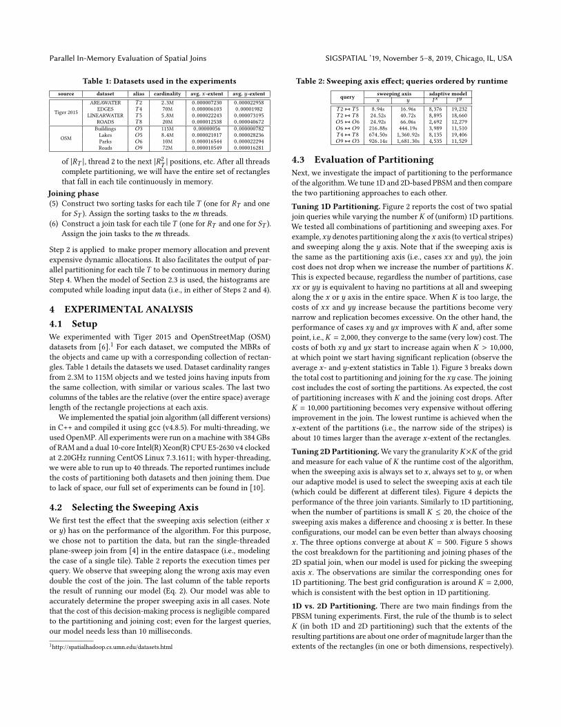
4 EXPERIMENTAL ANALYSIS4.1 SetupWe experimented with Tiger 2015 and OpenStreetMap (OSM)datasets from [6].1 For each dataset, we computed the MBRs ofthe objects and came up with a corresponding collection of rectan-gles. Table 1 details the datasets we used. Dataset cardinality rangesfrom 2.3M to 115M objects and we tested joins having inputs fromthe same collection, with similar or various scales. The last twocolumns of the tables are the relative (over the entire space) averagelength of the rectangle projections at each axis.

We implemented the spatial join algorithm (all di�erent versions)in C++ and compiled it using gcc (v4.8.5). For multi-threading, weused OpenMP. All experiments were run on amachine with 384 GBsof RAM and a dual 10-core Intel(R) Xeon(R) CPU E5-2630 v4 clockedat 2.20GHz running CentOS Linux 7.3.1611; with hyper-threading,we were able to run up to 40 threads. The reported runtimes includethe costs of partitioning both datasets and then joining them. Dueto lack of space, our full set of experiments can be found in [10].

4.2 Selecting the Sweeping AxisWe �rst test the e�ect that the sweeping axis selection (either xor �) has on the performance of the algorithm. For this purpose,we chose not to partition the data, but ran the single-threadedplane-sweep join from [4] in the entire dataspace (i.e., modelingthe case of a single tile). Table 2 reports the execution times perquery. We observe that sweeping along the wrong axis may evendouble the cost of the join. The last column of the table reportsthe result of running our model (Eq. 2). Our model was able toaccurately determine the proper sweeping axis in all cases. Notethat the cost of this decision-making process is negligible comparedto the partitioning and joining cost; even for the largest queries,our model needs less than 10 milliseconds.1http://spatialhadoop.cs.umn.edu/datasets.html

Table 2: Sweeping axis e�ect; queries ordered by runtime

query sweeping axis adaptive modelx � Ix I�

T 2 ./ T 5 8.94s 16.96s 8,376 19,232T 2 ./ T 8 24.52s 40.72s 8,895 18,660O5 ./ O6 24.92s 66.06s 2,692 12,279O6 ./ O9 216.88s 444.19s 3,989 11,510T 4 ./ T 8 674.50s 1,360.92s 8,135 19,406O9 ./ O3 926.14s 1,681.30s 4,535 11,529

4.3 Evaluation of PartitioningNext, we investigate the impact of partitioning to the performanceof the algorithm.We tune 1D and 2D-based PBSM and then comparethe two partitioning approaches to each other.

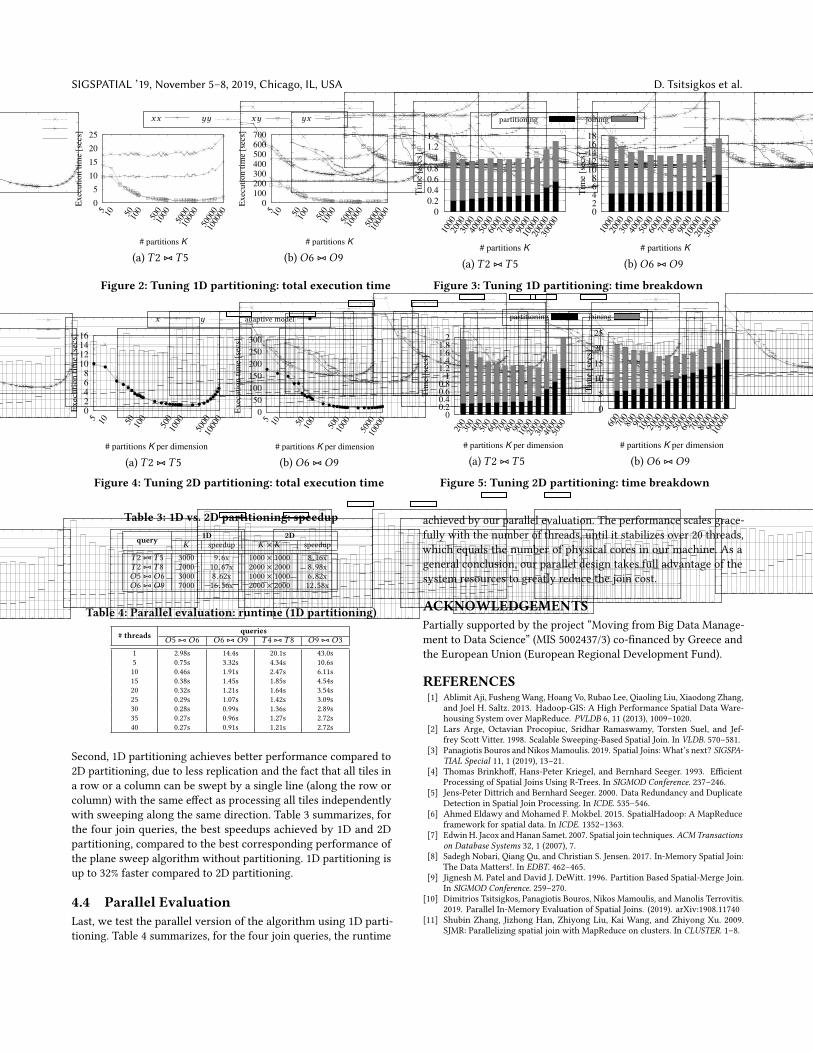
Tuning 1D Partitioning. Figure 2 reports the cost of two spatialjoin queries while varying the number K of (uniform) 1D partitions.We tested all combinations of partitioning and sweeping axes. Forexample, x� denotes partitioning along the x axis (to vertical stripes)and sweeping along the � axis. Note that if the sweeping axis isthe same as the partitioning axis (i.e., cases xx and ��), the joincost does not drop when we increase the number of partitions K .This is expected because, regardless the number of partitions, casexx or �� is equivalent to having no partitions at all and sweepingalong the x or � axis in the entire space. When K is too large, thecosts of xx and �� increase because the partitions become verynarrow and replication becomes excessive. On the other hand, theperformance of cases x� and �x improves with K and, after somepoint, i.e.,K = 2,000, they converge to the same (very low) cost. Thecosts of both x� and �x start to increase again when K > 10,000,at which point we start having signi�cant replication (observe theaverage x- and �-extent statistics in Table 1). Figure 3 breaks downthe total cost to partitioning and joining for the x� case. The joiningcost includes the cost of sorting the partitions. As expected, the costof partitioning increases with K and the joining cost drops. AfterK = 10,000 partitioning becomes very expensive without o�eringimprovement in the join. The lowest runtime is achieved when thex-extent of the partitions (i.e., the narrow side of the stripes) isabout 10 times larger than the average x-extent of the rectangles.

Tuning 2DPartitioning.We vary the granularityK⇥K of the gridand measure for each value of K the runtime cost of the algorithm,when the sweeping axis is always set to x , always set to �, or whenour adaptive model is used to select the sweeping axis at each tile(which could be di�erent at di�erent tiles). Figure 4 depicts theperformance of the three join variants. Similarly to 1D partitioning,when the number of partitions is small K 20, the choice of thesweeping axis makes a di�erence and choosing x is better. In thesecon�gurations, our model can be even better than always choosingx . The three options converge at about K = 500. Figure 5 showsthe cost breakdown for the partitioning and joining phases of the2D spatial join, when our model is used for picking the sweepingaxis x . The observations are similar the corresponding ones for1D partitioning. The best grid con�guration is around K = 2,000,which is consistent with the best option in 1D partitioning.

1D vs. 2D Partitioning. There are two main �ndings from thePBSM tuning experiments. First, the rule of the thumb is to selectK (in both 1D and 2D partitioning) such that the extents of theresulting partitions are about one order ofmagnitude larger than theextents of the rectangles (in one or both dimensions, respectively).

SIGSPATIAL ’19, November 5–8, 2019, Chicago, IL, USA D. Tsitsigkos et al.

xx

0 2 4 6 8

10 12 14 16

5 10 50 100

500

1000

5000

1000

0

Exec

uti

on t

ime

[sec

s]

# partitions K per dimension

yxa

0 5

10 15 20 25 30 35

5 10 50 100

500

1000

5000

1000

0

Exec

uti

on t

ime

[sec

s]# partitions K per dimension

yxa

0

5

10

15

20

25

30

5 10 50 100

500

1000

5000

1000

0

Exec

uti

on t

ime

[sec

s]


yxa

0

50

100

150

200

250

300

5 10 50 100

500

1000

5000

1000

0

Exec

uti

on t

ime

[sec

s]


yxa

T 2 ./ T 5 T 2 ./ T 8 O5 ./ O6 O6 ./ O9

Figure 8: Tuning 2D partitioning.

partitioning joining

0 0.2 0.4 0.6 0.8

1 1.2 1.4 1.6 1.8

2

200

300

400

500

600

700

800

900

1000

2000

3000

4000

5000

Tim

e [s

ecs]


0 0.5

1 1.5

2 2.5

3 3.5

4 4.5

5

200

300

400

500

600

700

800

900

1000

2000

3000

4000

5000

Tim

e [s

ecs]


0

1

2

3

4

5

6

200

300

400

500

600

700

800

900

1000

2000

3000

4000

5000

Tim

e [s

ecs]


0

5

10

15

20

25

600

700

800

900

1000

2000

3000

4000

5000

6000

7000

8000

9000

1000

0

Tim

e [s

ecs]


(a) T 2 ./ T 5 (b) T 2 ./ T 8 (c) O5 ./ O6 (d) O6 ./ O9

Figure 9: Tuning 2D partitioning: time breakdown

[5] Thomas Brinkho�, Hans-Peter Kriegel, and Bernhard Seeger. 1993. E�cientProcessing of Spatial Joins Using R-Trees. In SIGMOD Conference. 237–246.

[6] Huiping Cao, Nikos Mamoulis, and DavidW. Cheung. 2007. Discovery of PeriodicPatterns in Spatiotemporal Sequences. IEEE Trans. Knowl. Data Eng. 19, 4 (2007),453–467.

[7] Jens-Peter Dittrich and Bernhard Seeger. 2000. Data Redundancy and DuplicateDetection in Spatial Join Processing. In ICDE. 535–546.

[8] Ahmed Eldawy and Mohamed F. Mokbel. 2015. SpatialHadoop: A MapReduceframework for spatial data. In ICDE. 1352–1363.

[9] Martin Ester, Hans-Peter Kriegel, Jörg Sander, and Xiaowei Xu. 1996. A Density-Based Algorithm for Discovering Clusters in Large Spatial Databases with Noise.In Proceedings of the Second International Conference on Knowledge Discovery andData Mining (KDD-96), Portland, Oregon, USA. 226–231.

[10] Ralf Hartmut Güting. 1994. An Introduction to Spatial Database Systems. VLDBJournal 3, 4 (1994), 357–399.

[11] Antonin Guttman. 1984. R-Trees: A Dynamic Index Structure for Spatial Search-ing. In SIGMOD Conference. 47–57.

[12] EdwinH. Jacox andHanan Samet. 2007. Spatial join techniques. ACMTransactionson Database Systems 32, 1 (2007), 7.

[13] Andreas Kipf, Harald Lang, Varun Pandey, Raul Alexandru Persa, Peter A. Boncz,Thomas Neumann, and Alfons Kemper. 2018. Adaptive Geospatial Joins forModern Hardware. CoRR abs/1802.09488 (2018). http://arxiv.org/abs/1802.09488

[14] Nick Koudas and Kenneth C. Sevcik. 1997. Size Separation Spatial Join. In SIGMODConference. 324–335.

[15] Scott T. Leutenegger, J. M. Edgington, and Mario A. López. 1997. STR: A Simpleand E�cient Algorithm for R-Tree Packing. In ICDE. 497–506.

[16] Ming-Ling Lo and Chinya V. Ravishankar. 1996. Spatial Hash-Joins. In SIGMODConference. 247–258.

[17] Paul A. Longley, Mike Goodchild, David J. Maguire, and David W. Rhind. 2010.Geographic Information Systems and Science (3rd ed.). Wiley Publishing.

[18] Sadegh Nobari, Qiang Qu, and Christian S. Jensen. 2017. In-Memory Spatial Join:The Data Matters!. In EDBT. 462–465.

[19] Sadegh Nobari, Farhan Tauheed, Thomas Heinis, Panagiotis Karras, StéphaneBressan, and Anastasia Ailamaki. 2013. TOUCH: in-memory spatial join byhierarchical data-oriented partitioning. In SIGMOD Conference. 701–712.

[20] Varun Pandey, Andreas Kipf, Thomas Neumann, and Alfons Kemper. 2018. HowGood Are Modern Spatial Analytics Systems? PVLDB 11, 11 (2018), 1661–1673.

[21] Jignesh M. Patel and David J. DeWitt. 1996. Partition Based Spatial-Merge Join.In SIGMOD Conference. 259–270.

[22] Mirjana Pavlovic, Thomas Heinis, Farhan Tauheed, Panagiotis Karras, and Anas-tasia Ailamaki. 2016. TRANSFORMERS: Robust spatial joins on non-uniformdata distributions. In ICDE. 673–684.

[23] Mirjana Pavlovic, Farhan Tauheed, Thomas Heinis, and Anastasia Ailamaki. 2013.GIPSY: joining spatial datasets with contrasting density. In SSDBM.

[24] Franco P. Preparata and Michael Ian Shamos. 1985. Computational Geometry -An Introduction. Springer.

[25] Suprio Ray, Bogdan Simion, Angela Demke Brown, and Ryan Johnson. 2014.Skew-resistant parallel in-memory spatial join. In SSDBM. 6:1–6:12.

[26] Ibrahim Sabek and Mohamed F. Mokbel. 2017. On Spatial Joins in MapReduce.In SIGSPATIAL/GIS.

[27] Farhan Tauheed, Thomas Heinis, and Anastasia Ailamaki. 2015. Con�guringSpatial Grids for E�cient Main Memory Joins. In BICOD.

[28] Dong Xie, Feifei Li, Bin Yao, Gefei Li, Zhongpu Chen, Liang Zhou, and Minyi Guo.2016. Simba: spatial in-memory big data analysis. In SIGSPATIAL/GIS. 86:1–86:4.

[29] Simin You, Jianting Zhang, and Le Gruenwald. 2015. Large-scale spatial joinquery processing in Cloud. In CloudDB, ICDE Workshops. 34–41.

[30] Jia Yu, Jinxuan Wu, and Mohamed Sarwat. 2015. GeoSpark: a cluster computingframework for processing large-scale spatial data. In SIGSPATIAL/GIS. 70:1–70:4.

[31] Shubin Zhang, Jizhong Han, Zhiyong Liu, Kai Wang, and Zhiyong Xu. 2009.SJMR: Parallelizing spatial join with MapReduce on clusters. In CLUSTER. 1–8.

[32] Xiaofang Zhou, David J. Abel, and David Tru�et. 1997. Data Partitioning forParallel Spatial Join Processing. In SSD. 178–196.

��

0 2 4 6 8

10 12 14 16

5 10 50 100

500

1000

5000

1000

0

Exec

uti

on t

ime

[sec

s]


yxa

0 5

10 15 20 25 30 35

5 10 50 100

500

1000

5000

1000

0

Exec

uti

on t

ime

[sec

s]


yxa

0

5

10

15

20

25

30

5 10 50 100

500

1000

5000

1000

0

Exec

uti

on t

ime

[sec

s]


yxa

0

50

100

150

200

250

300

5 10 50 100

500

1000

5000

1000

0

Exec

uti

on t

ime

[sec

s]


yxa

T 2 ./ T 5 T 2 ./ T 8 O5 ./ O6 O6 ./ O9



0 0.2 0.4 0.6 0.8

1 1.2 1.4 1.6 1.8

2

200

300

400

500

600

700

800

900

1000

2000

3000

4000

5000

Tim

e [s

ecs]


0 0.5

1 1.5

2 2.5

3 3.5

4 4.5

5

200

300

400

500

600

700

800

900

1000

2000

3000

4000

5000

Tim

e [s

ecs]


0

1

2

3

4

5

6

200

300

400

500

600

700

800

900

1000

2000

3000

4000

5000

Tim

e [s

ecs]


0

5

10

15

20

25

600

700

800

900

1000

2000

3000

4000

5000

6000

7000

8000

9000

1000

0

Tim

e [s

ecs]


(a) T 2 ./ T 5 (b) T 2 ./ T 8 (c) O5 ./ O6 (d) O6 ./ O9






























x�

0

5

10

15

20

25

5 10 50 100

500

1000

5000

1000

050

000

1000

00

Exec

uti

on t

ime

[sec

s]

# partitions K

y-yx-xx-yy-xx-ay-a

0

10

20

30

40

50

60

5 10 50 100

500

1000

5000

1000

050

000

1000

00

Exec

uti

on t

ime

[sec

s]

# partitions K

0 10 20 30 40 50 60 70 80 90

100

5 10 50100

500

1000

5000

1000

050

000

1000

00

Exec

uti

on t

ime

[sec

s]

# partitions K

0 100 200 300 400 500 600 700

5 10 50100

500

1000

5000

1000

050

000

1000

00

Exec

uti

on t

ime

[sec

s]

# partitions K

(a) T 2 ./ T 5 (b) T 2 ./ T 8 (c) O5 ./ O6 (d) O6 ./ O9

Figure 6: Tuning 1D partitioning: total execution time


0 0.2 0.4 0.6 0.8

1 1.2 1.4

1000

2000

3000

4000

5000

6000

7000

8000

9000

1000

020

000

3000

0

Tim

e [s

ecs]

# partitions K

0

0.5

1

1.5

2

2.5

3

1000

2000

3000

4000

5000

6000

7000

8000

9000

1000

020

000

3000

0

Tim

e [s

ecs]

# partitions K

0 0.5

1 1.5

2 2.5

3 3.5

4 4.5

5

1000

2000

3000

4000

5000

6000

7000

8000

9000

1000

020

000

3000

0

Tim

e [s

ecs]

# partitions K

0 2 4 6 8

10 12 14 16 18

1000

2000

3000

4000

5000

6000

7000

8000

9000

1000

020

000

3000

0

Tim

e [s

ecs]

# partitions K

(a) T 2 ./ T 5 (b) T 2 ./ T 8 (c) O5 ./ O6 (d) O6 ./ O9


tiles). Again, we used the GDT approach for duplicate avoidance.Figure 8 plots the performance of the three join variants. The obser-vations regarding the choice of the sweeping axis and the numberof partitions are similar to the cases of 1D partitioning. Speci�cally,when the number of partitions is small K 20, the choice of thesweeping axis makes a di�erence and choosing x is better. In thesecon�gurations, our model can be even better than always choosingx . The three options converge at about K = 500 and there are nosigni�cant di�erences between them after this point.

Figure 9 shows the cost breakdown for the partitioning andjoining phases of the 2D spatial join, when our model is used forpicking the sweeping axis x . As in the case of 1D joins, we observethat the cost of partitioning increases with K and becomes toohigh when the tiles become too many and very small (i.e., whenK > 2,000). On the other hand, the join cost drops, but stabilizesafterK > 2,000. After this point, the numberK⇥K of tiles (that haveto be managed) becomes extremely high and replication becomesexcessive. The joining phase does not bene�t; due to replication,the join inputs at each tile do not reduce in size and the same joinresults are computed in neighboring tiles.

The best grid con�guration is around K = 2,000, which is con-sistent with the best option in 1D partitioning. Hence, the rule ofthe thumb is to select K (in both 1D and 2D partitioning) suchthat the extents of the resulting partitions are about one order ofmagnitude larger than the extents of the rectangles (in one or bothdimensions, respectively). In the rest of the experiments, we use thisrule to select K as the default number of divisions in the splitting

dimension(s). Also, we always use our adaptive model to select thesweeping axis.

4.5 Duplicate AvoidanceWe now test the

4.6 Parallel Evaluation++ compare join-only cost, assuming that data are already parti-tioned as in a data management system (e.g. SpatialHadoop) whichuses the grid as an index for queries. See if mj could beat ditt inthis case.

5 CONCLUSIONSIn this paper, we have investigated directions towards tuning aclassic and popular partitioning-based spatial join algorithm, whichis typically used for in-memory and parallel/distributed join evalu-ation. [nikos: to be completed]

Directions for future work include consideration of the re�ne-ment step of the join, which can be signi�cantly more expensivethan the �lter step. In addition, we plan to adapt our techniquesand investigate their performance in a distributed environment andfor the case of NUMA architectures.

REFERENCES[1] Ablimit Aji, FushengWang, Hoang Vo, Rubao Lee, Qiaoling Liu, Xiaodong Zhang,

and Joel H. Saltz. 2013. Hadoop-GIS: A High Performance Spatial Data Ware-housing System over MapReduce. PVLDB 6, 11 (2013), 1009–1020.

[2] Lars Arge, Octavian Procopiuc, Sridhar Ramaswamy, Torsten Suel, and Jef-frey Scott Vitter. 1998. Scalable Sweeping-Based Spatial Join. In VLDB. 570–581.

�x

0

5

10

15

20

25

5 10 50 100

500

1000

5000

1000

050

000

1000

00

Exec

uti

on t

ime

[sec

s]

# partitions K

y-yx-yy-xx-ay-a

0

10

20

30

40

50

60

5 10 50 100

500

1000

5000

1000

050

000

1000

00

Exec

uti

on t

ime

[sec

s]

# partitions K

0 10 20 30 40 50 60 70 80 90

100

5 10 50100

500

1000

5000

1000

050

000

1000

00

Exec

uti

on t

ime

[sec

s]

# partitions K

0 100 200 300 400 500 600 700

5 10 50100

500

1000

5000

1000

050

000

1000

00

Exec

uti

on t

ime

[sec

s]

# partitions K

(a) T 2 ./ T 5 (b) T 2 ./ T 8 (c) O5 ./ O6 (d) O6 ./ O9



0 0.2 0.4 0.6 0.8

1 1.2 1.4

1000

2000

3000

4000

5000

6000

7000

8000

9000

1000

020

000

3000

0

Tim

e [s

ecs]

# partitions K

0

0.5

1

1.5

2

2.5

3

1000

2000

3000

4000

5000

6000

7000

8000

9000

1000

020

000

3000

0

Tim

e [s

ecs]

# partitions K

0 0.5

1 1.5

2 2.5

3 3.5

4 4.5

5

1000

2000

3000

4000

5000

6000

7000

8000

9000

1000

020

000

3000

0

Tim

e [s

ecs]

# partitions K

0 2 4 6 8

10 12 14 16 18

1000

2000

3000

4000

5000

6000

7000

8000

9000

1000

020

000

3000

0

Tim

e [s

ecs]

# partitions K

(a) T 2 ./ T 5 (b) T 2 ./ T 8 (c) O5 ./ O6 (d) O6 ./ O9


tiles). Again, we used the GDT approach for duplicate avoidance.Figure 8 plots the performance of the three join variants. The obser-vations regarding the choice of the sweeping axis and the numberof partitions are similar to the cases of 1D partitioning. Speci�cally,when the number of partitions is small K 20, the choice of thesweeping axis makes a di�erence and choosing x is better. In thesecon�gurations, our model can be even better than always choosingx . The three options converge at about K = 500 and there are nosigni�cant di�erences between them after this point.

Figure 9 shows the cost breakdown for the partitioning andjoining phases of the 2D spatial join, when our model is used forpicking the sweeping axis x . As in the case of 1D joins, we observethat the cost of partitioning increases with K and becomes toohigh when the tiles become too many and very small (i.e., whenK > 2,000). On the other hand, the join cost drops, but stabilizesafterK > 2,000. After this point, the numberK⇥K of tiles (that haveto be managed) becomes extremely high and replication becomesexcessive. The joining phase does not bene�t; due to replication,the join inputs at each tile do not reduce in size and the same joinresults are computed in neighboring tiles.

The best grid con�guration is around K = 2,000, which is con-sistent with the best option in 1D partitioning. Hence, the rule ofthe thumb is to select K (in both 1D and 2D partitioning) suchthat the extents of the resulting partitions are about one order ofmagnitude larger than the extents of the rectangles (in one or bothdimensions, respectively). In the rest of the experiments, we use thisrule to select K as the default number of divisions in the splitting

dimension(s). Also, we always use our adaptive model to select thesweeping axis.

4.5 Duplicate AvoidanceWe now test the

4.6 Parallel Evaluation++ compare join-only cost, assuming that data are already parti-tioned as in a data management system (e.g. SpatialHadoop) whichuses the grid as an index for queries. See if mj could beat ditt inthis case.

5 CONCLUSIONSIn this paper, we have investigated directions towards tuning aclassic and popular partitioning-based spatial join algorithm, whichis typically used for in-memory and parallel/distributed join evalu-ation. [nikos: to be completed]

Directions for future work include consideration of the re�ne-ment step of the join, which can be signi�cantly more expensivethan the �lter step. In addition, we plan to adapt our techniquesand investigate their performance in a distributed environment andfor the case of NUMA architectures.




0

5

10

15

20

25

5 10 50 100

500

1000

5000

1000

050

000

1000

00

Exec

uti

on t

ime

[sec

s]

# partitions K

0 100 200 300 400 500 600 700

5 10 50100

500

1000

5000

1000

050

000

1000

00

Exec

uti

on t

ime

[sec

s]# partitions K

(a) T 2 ./ T 5 (b) O6 ./ O9



0 0.2 0.4 0.6 0.8

1 1.2 1.4

1000

2000

3000

4000

5000

6000

7000

8000

9000

1000

020

000

3000

0

Tim

e [s

ecs]

# partitions K

0 2 4 6 8

10 12 14 16 18

1000

2000

3000

4000

5000

6000

7000

8000

9000

1000

020

000

3000

0

Tim

e [s

ecs]

# partitions K

(a) T 2 ./ T 5 (b) O6 ./ O9


x

0 2 4 6 8

10 12 14 16

5 10 50 100

500

1000

5000

1000

0

Exec

uti

on t

ime

[sec

s]


yxa

0 5

10 15 20 25 30 35

5 10 50 100

500

1000

5000

1000

0

Exec

uti

on t

ime

[sec

s]


yxa

0

5

10

15

20

25

30

5 10 50 100

500

1000

5000

1000

0

Exec

uti

on t

ime

[sec

s]


yxa

0

50

100

150

200

250

300

5 10 50 100

500

1000

5000

1000

0

Exec

uti

on t

ime

[sec

s]


yxa

T 2 ./ T 5 T 2 ./ T 8 O5 ./ O6 O6 ./ O9



0 0.2 0.4 0.6 0.8

1 1.2 1.4 1.6 1.8

2

200

300

400

500

600

700

800

900

1000

2000

3000

4000

5000

Tim

e [s

ecs]


0 0.5

1 1.5

2 2.5

3 3.5

4 4.5

5

200

300

400

500

600

700

800

900

1000

2000

3000

4000

5000

Tim

e [s

ecs]


0

1

2

3

4

5

6

200

300

400

500

600

700

800

900

1000

2000

3000

4000

5000

Tim

e [s

ecs]


0

5

10

15

20

25

600

700

800

900

1000

2000

3000

4000

5000

6000

7000

8000

9000

1000

0

Tim

e [s

ecs]


(a) T 2 ./ T 5 (b) T 2 ./ T 8 (c) O5 ./ O6 (d) O6 ./ O9






























�

0 2 4 6 8

10 12 14 16

5 10 50 100

500

1000

5000

1000

0

Exec

uti

on t

ime

[sec

s]


yxa

0 5

10 15 20 25 30 35

5 10 50 100

500

1000

5000

1000

0

Exec

uti

on t

ime

[sec

s]


yxa

0

5

10

15

20

25

30

5 10 50 100

500

1000

5000

1000

0

Exec

uti

on t

ime

[sec

s]


yxa

0

50

100

150

200

250

300

5 10 50 100

500

1000

5000

1000

0

Exec

uti

on t

ime

[sec

s]# partitions K per dimension

yxa

T 2 ./ T 5 T 2 ./ T 8 O5 ./ O6 O6 ./ O9



0 0.2 0.4 0.6 0.8

1 1.2 1.4 1.6 1.8

2

200

300

400

500

600

700

800

900

1000

2000

3000

4000

5000

Tim

e [s

ecs]


0 0.5

1 1.5

2 2.5

3 3.5

4 4.5

5

200

300

400

500

600

700

800

900

1000

2000

3000

4000

5000

Tim

e [s

ecs]


0

1

2

3

4

5

6

200

300

400

500

600

700

800

900

1000

2000

3000

4000

5000

Tim

e [s

ecs]


0

5

10

15

20

25

600

700

800

900

1000

2000

3000

4000

5000

6000

7000

8000

9000

1000

0

Tim

e [s

ecs]


(a) T 2 ./ T 5 (b) T 2 ./ T 8 (c) O5 ./ O6 (d) O6 ./ O9






























adaptive model

0 2 4 6 8

10 12 14 16

5 10 50 100

500

1000

5000

1000

0

Exec

uti

on t

ime

[sec

s]


yxa

0 5

10 15 20 25 30 35

5 10 50 100

500

1000

5000

1000

0

Exec

uti

on t

ime

[sec

s]


yxa

0

5

10

15

20

25

30

5 10 50 100

500

1000

5000

1000

0

Exec

uti

on t

ime

[sec

s]


yxa

0

50

100

150

200

250

300

5 10 50 100

500

1000

5000

1000

0

Exec

uti

on t

ime

[sec

s]


yxa

T 2 ./ T 5 T 2 ./ T 8 O5 ./ O6 O6 ./ O9



0 0.2 0.4 0.6 0.8

1 1.2 1.4 1.6 1.8

2

200

300

400

500

600

700

800

900

1000

2000

3000

4000

5000

Tim

e [s

ecs]


0 0.5

1 1.5

2 2.5

3 3.5

4 4.5

5

200

300

400

500

600

700

800

900

1000

2000

3000

4000

5000

Tim

e [s

ecs]


0

1

2

3

4

5

6

200

300

400

500

600

700

800

900

1000

2000

3000

4000

5000

Tim

e [s

ecs]


0

5

10

15

20

25

600

700

800

900

1000

2000

3000

4000

5000

6000

7000

8000

9000

1000

0

Tim

e [s

ecs]


(a) T 2 ./ T 5 (b) T 2 ./ T 8 (c) O5 ./ O6 (d) O6 ./ O9






























0 2 4 6 8

10 12 14 16

5 10 50 100

500

1000

5000

1000

0

Exec

uti

on t

ime

[sec

s]


0

50

100

150

200

250

300

5 10 50 100

500

1000

5000

1000

0

Exec

uti

on t

ime

[sec

s]


(a) T 2 ./ T 5 (b) O6 ./ O9



0 0.2 0.4 0.6 0.8

1 1.2 1.4 1.6 1.8

2

200

300

400

500

600

700

800

900

1000

2000

3000

4000

5000

Tim

e [s

ecs]


0

5

10

15

20

25

600

700

800

900

1000

2000

3000

4000

5000

6000

7000

8000

9000

1000

0

Tim

e [s

ecs]


(a) T 2 ./ T 5 (b) O6 ./ O9


Table 3: 1D vs. 2D partitioning: speedup

query 1D 2DK speedup K ⇥ K speedup

T 2 ./ T 5 3000 9.6x 1000 ⇥ 1000 8.16xT 2 ./ T 8 7000 10.67x 2000 ⇥ 2000 8.98xO5 ./ O6 3000 8.62x 1000 ⇥ 1000 6.82xO6 ./ O9 7000 16.56x 2000 ⇥ 2000 12.58x

Table 4: Parallel evaluation: runtime (1D partitioning)

# threads queriesO5 ./ O6 O6 ./ O9 T 4 ./ T 8 O9 ./ O3

1 2.98s 14.4s 20.1s 43.0s5 0.75s 3.32s 4.34s 10.6s10 0.46s 1.91s 2.47s 6.11s15 0.38s 1.45s 1.85s 4.54s20 0.32s 1.21s 1.64s 3.54s25 0.29s 1.07s 1.42s 3.09s30 0.28s 0.99s 1.36s 2.89s35 0.27s 0.96s 1.27s 2.72s40 0.27s 0.91s 1.21s 2.72s

Second, 1D partitioning achieves better performance compared to2D partitioning, due to less replication and the fact that all tiles ina row or a column can be swept by a single line (along the row orcolumn) with the same e�ect as processing all tiles independentlywith sweeping along the same direction. Table 3 summarizes, forthe four join queries, the best speedups achieved by 1D and 2Dpartitioning, compared to the best corresponding performance ofthe plane sweep algorithm without partitioning. 1D partitioning isup to 32% faster compared to 2D partitioning.

4.4 Parallel EvaluationLast, we test the parallel version of the algorithm using 1D parti-tioning. Table 4 summarizes, for the four join queries, the runtime

achieved by our parallel evaluation. The performance scales grace-fully with the number of threads, until it stabilizes over 20 threads,which equals the number of physical cores in our machine. As ageneral conclusion, our parallel design takes full advantage of thesystem resources to greatly reduce the join cost.

ACKNOWLEDGEMENTSPartially supported by the project “Moving from Big Data Manage-ment to Data Science” (MIS 5002437/3) co-�nanced by Greece andthe European Union (European Regional Development Fund).




[3] Panagiotis Bouros and Nikos Mamoulis. 2019. Spatial Joins: What’s next? SIGSPA-TIAL Special 11, 1 (2019), 13–21.







[10] Dimitrios Tsitsigkos, Panagiotis Bouros, Nikos Mamoulis, and Manolis Terrovitis.2019. Parallel In-Memory Evaluation of Spatial Joins. (2019). arXiv:1908.11740


http://arxiv.org/abs/1908.11740

parallel in-memory evaluation of spatial joins

Documents