parallel and in-memory big spatial data processing systems
TRANSCRIPT

Parallel and In-Memory Big Spatial
Data Processing Systems and Benchmarking
by
Md. Mahbub Alam
Bachelor of Computer Science and Engineering,Dhaka University of Engineering & Technology-Gazipur, 2009
A THESIS SUBMITTED IN PARTIAL FULFILLMENT OFTHE REQUIREMENTS FOR THE DEGREE OF
Master of Computer Science
In the Graduate Academic Unit of Computer Science
Supervisor(s): Suprio Ray, PhD, Computer ScienceVirendrakumar C. Bhavsar, PhD, Computer Science
Examining Board: Gerhard Dueck, PhD, Computer Science, ChairpersonWeichang Du, PhD, Computer ScienceS. A. Saleh, PhD, Electrical Engineering
This thesis is accepted
Dean of Graduate Studies
THE UNIVERSITY OF NEW BRUNSWICK
December, 2018
c©Md. Mahbub Alam, 2019

Abstract
With the accelerated growth in spatial data volume, being generated from
a wide variety of sources, the need for efficient storage, retrieval, processing
and analyzing of spatial data is ever more important. Hence, the spatial data
processing system has become an important field of research. Though the
traditional relational database systems provide spatial functionality (such as,
PostgreSQL with PostGIS), due to the lack of parallelism and I/O bottle-
neck, these systems are not efficient to run compute-intensive spatial queries
on large datasets. In recent times a number of big spatial data systems
have been proposed by researchers around the world. These systems can
be roughly categorized into disk-based systems over Apache Hadoop and in-
memory systems based on Apache Spark. The available features supported by
these systems vary widely. However, there has not been any comprehensive
evaluation study of these systems in terms of performance, scalability, and
functionality. In order to address this need, this thesis proposes a benchmark
to evaluate big spatial data systems. It intends to investigate the present sta-
tus of the big spatial data systems by conducting a comprehensive feature
ii

analysis and performance evaluation of a few representative systems.
The Hadoop and Spark based big spatial data systems are distributed, scal-
able, and able to exploit the parallelism of today’s multi-core/many-core
architecture. However, most of them are immature, unstable, difficult to
extend and missing efficient query language like SQL. In this work, a disk-
based system Parallax is introduced as a parallel big spatial database sys-
tem. It integrates the powerful spatial features of PostgreSQL/PostGIS and
distributed persistence storage of Alluxio. The host-specific data partitioning
and parallel query on local data in each node ensure the maximum utiliza-
tion of main memory, disk storage, and CPU. This thesis also introduces an
in-memory system SpatialIgnite, as extended spatial support for Apache Ig-
nite. SpatialIgnite incorporates a spatial library which contains all the OGC
compliant join predicates and spatial analysis functions. Along with query
parallelism and collocated query processing of Ignite, the integrated spatial
data partitioning techniques improve the performance of SpatialIgnite. The
evaluation shows that SpatialIgnite performs better than Hadoop and Spark
based systems.
iii

Acknowledgements
First of all, I would like to express my profound gratitude to the almighty
who bestowed self-confidence, ability, and strength in me to complete my
master’s study and research.
I would like to express my sincere gratitude to my supervisor, Dr. Suprio
Ray, and Dr. Virendrakumar C. Bhavsar, for their helpful guidance, encour-
agement, and expert advice throughout all stages of my study and research.
I could not have imagined having better supervisors for my master’s study.
Besides my supervisors, I would like to thank my thesis committee, Dr. Ger-
hard Dueck, Dr. Weichang Du, Dr. S. A. Saleh, and Dr. Patricia Evans for
their insightful comments and encouragement.
I would like to thank my fellow lab mates, Alex Watson, Divya Negi, Puya
Memarzia and Yoan Arseneau for their support, and friendship. I would also
like to give special thanks to my friends and fellow country mates. Without
your help and encouragement, it would have been difficult for me to stay
abroad. I had a lovely time with you during my two years of study at UNB.
I am sincerely grateful to my parents, lovely wife, and daughter for their
iv
cooperation and support. I will never forget their positive influence on my
study during the time that I was far from home.
Finally, I would like to thank the Natural Sciences and Engineering Re-
search Council (NSERC), Canada, the New Brunswick Innovation Founda-
tion (NBIF), NB, Canada, and the University of New Brunswick, Frederic-
ton, NB, Canada for financially supporting my study and research. Special
thanks to authors of different references used for the research.
v
Table of Contents
Abstract ii
Acknowledgments iv
Table of Contents ix
List of Tables x
List of Figures xii
Abbreviations xiii
1 Introduction 1
1.1 Motivations . . . . . . . . . . . . . . . . . . . . . . . . . . . . 6
1.2 Contributions . . . . . . . . . . . . . . . . . . . . . . . . . . . 8
1.3 Thesis Outline . . . . . . . . . . . . . . . . . . . . . . . . . . . 9
2 Background 10
2.1 Geospatial Big Data: Challenges and Opportunities . . . . . . 10
2.2 Spatial Query Processing . . . . . . . . . . . . . . . . . . . . . 12
vi

2.3 Spatial Operations . . . . . . . . . . . . . . . . . . . . . . . . 15
2.4 Distributed In-Memory Data Processing Systems . . . . . . . 17
2.4.1 Data Partitioning in Apache Ignite . . . . . . . . . . . 20
2.5 Parallel Spatial Data Processing Systems . . . . . . . . . . . . 22
2.5.1 PostgreSQL Foreign Data Wrapper . . . . . . . . . . . 23
2.5.2 Alluxio: A Virtual Distributed File System . . . . . . . 24
3 SpatialIgnite: Extended Spatial Support for Apache Ignite 27
3.1 Introduction . . . . . . . . . . . . . . . . . . . . . . . . . . . . 27
3.2 Architecture . . . . . . . . . . . . . . . . . . . . . . . . . . . . 28
3.3 Supported Spatial Features . . . . . . . . . . . . . . . . . . . . 29
3.4 Spatial Data Partitioning . . . . . . . . . . . . . . . . . . . . . 30
3.5 Data Persistence . . . . . . . . . . . . . . . . . . . . . . . . . 33
3.6 Performance Evaluation . . . . . . . . . . . . . . . . . . . . . 35
3.6.1 Experimental Setup . . . . . . . . . . . . . . . . . . . . 35
3.6.2 Result Analysis and Discussion . . . . . . . . . . . . . 36
3.7 Summary . . . . . . . . . . . . . . . . . . . . . . . . . . . . . 40
4 Benchmarking Big Spatial Data Processing Systems 41
4.1 Introduction . . . . . . . . . . . . . . . . . . . . . . . . . . . . 41
4.2 Related Work . . . . . . . . . . . . . . . . . . . . . . . . . . . 43
4.3 Hadoop-based Big Spatial Data Systems . . . . . . . . . . . . 45
4.4 Distributed In-Memory Big Spatial Data Systems . . . . . . . 48
4.4.1 Spark-based Big Spatial Data Systems . . . . . . . . . 48
vii

4.4.2 Other Distributed In-memory Big Spatial Data Systems 53
4.5 Our Benchmark . . . . . . . . . . . . . . . . . . . . . . . . . . 54
4.5.1 Workload . . . . . . . . . . . . . . . . . . . . . . . . . 55
4.5.2 Datasets . . . . . . . . . . . . . . . . . . . . . . . . . . 56
4.6 Performance Evaluation . . . . . . . . . . . . . . . . . . . . . 56
4.6.1 Benchmark Implementation . . . . . . . . . . . . . . . 57
4.6.2 Experimental Setup . . . . . . . . . . . . . . . . . . . . 58
4.6.3 Result Analysis and Discussion . . . . . . . . . . . . . 58
4.7 Summary . . . . . . . . . . . . . . . . . . . . . . . . . . . . . 62
5 Parallax: A Parallel Big Spatial Database System 64
5.1 Introduction . . . . . . . . . . . . . . . . . . . . . . . . . . . . 64
5.2 Architecture . . . . . . . . . . . . . . . . . . . . . . . . . . . . 65
5.3 PostgreSQL Foreign Data Wrapper for Alluxio . . . . . . . . . 67
5.4 Host Specific Spatial Data Partitioning . . . . . . . . . . . . . 69
5.5 Query Execution in Parallax . . . . . . . . . . . . . . . . . . . 70
5.6 Performance Evaluation . . . . . . . . . . . . . . . . . . . . . 71
5.6.1 Experimental Setup . . . . . . . . . . . . . . . . . . . . 71
5.6.2 Result Analysis and Discussion . . . . . . . . . . . . . 72
5.6.3 Reasons of Performance Degradation . . . . . . . . . . 73
5.7 Summary . . . . . . . . . . . . . . . . . . . . . . . . . . . . . 74
6 Conclusions and Future Work 75
6.1 Thesis Contributions . . . . . . . . . . . . . . . . . . . . . . . 76
viii

6.2 Future Work . . . . . . . . . . . . . . . . . . . . . . . . . . . . 78
Bibliography 85
Vita
ix

List of Tables
3.1 Verification of Result Accuracy . . . . . . . . . . . . . . . . . 31
3.2 Workloads (further described in Section 4.5.1) . . . . . . . . . 34
3.3 Datasets description . . . . . . . . . . . . . . . . . . . . . . . 36
4.1 Hadoop-based Big Spatial Data Systems . . . . . . . . . . . . 47
4.2 Spark-based Big Spatial Data Systems . . . . . . . . . . . . . 49
4.3 Features of SpatialIgnite . . . . . . . . . . . . . . . . . . . . . 54
4.4 Existing Support of Spatial Join Predicates . . . . . . . . . . . 54
4.5 Existing Support of Spatial Analysis Functions . . . . . . . . . 55
4.6 Verification of Result Accuracy . . . . . . . . . . . . . . . . . 59
5.1 Spatial Join Queries (Parallax (SQL) vs SpatialHadoop (Pi-
geon)) . . . . . . . . . . . . . . . . . . . . . . . . . . . . . . . 72
5.2 Example of real life query . . . . . . . . . . . . . . . . . . . . 73
x

List of Figures
2.1 Example of two phase spatial query processing (source [40]) . 14
2.2 Topological relations from DE-9IM (source [40]) . . . . . . . . 14
2.3 Spatial attributes of points, lines and polygons (source: Wikipedia) 15
2.4 Matrix form of possible intersections of polygons (source: open-
geo.org) . . . . . . . . . . . . . . . . . . . . . . . . . . . . . . 16
2.5 DE-9IM matrix for ’polyline intersects polygon’ (source: open-
geo.org) . . . . . . . . . . . . . . . . . . . . . . . . . . . . . . 16
2.6 Ignite In-Memory Data Grid . . . . . . . . . . . . . . . . . . . 18
2.7 Example of Rendezvous Hashing . . . . . . . . . . . . . . . . . 21
2.8 Interaction of PostgreSQL with foreign data sources. . . . . . 24
2.9 Architectural overview of Alluxio . . . . . . . . . . . . . . . . 26
2.10 Interaction of Alluxio with storage layer . . . . . . . . . . . . 26
3.1 Architecture of SpatialIgnite . . . . . . . . . . . . . . . . . . . 28
3.2 Example of Grid Partitioning . . . . . . . . . . . . . . . . . . 31
3.3 Niharika spatial declustering (source: Niharika [32]) . . . . . . 32
xi

3.4 Speedup with the increase in the number of threads per node
(all joins involving points and polygons running on an 8-node
cluster) . . . . . . . . . . . . . . . . . . . . . . . . . . . . . . . 37
3.5 Speedup with the increase in the number of threads per node
(all joins involving lines running on an 8-node cluster) . . . . . 38
3.6 Spatial Join involving Points, Lines and Polygons (on an 8-
node cluster) . . . . . . . . . . . . . . . . . . . . . . . . . . . 39
3.7 Spatial Analysis queries involving Points, Lines and Polygons
(on an 8-node cluster) . . . . . . . . . . . . . . . . . . . . . . 39
3.8 Range queries involving Points, Lines and Polygons (on an
8-node cluster) . . . . . . . . . . . . . . . . . . . . . . . . . . 40
4.1 Spatial Join involving Points, Lines and Polygons (on an 8-
node cluster) . . . . . . . . . . . . . . . . . . . . . . . . . . . 60
4.2 Spatial Analysis queries involving Points, Lines and Polygons
(on an 8-node cluster) . . . . . . . . . . . . . . . . . . . . . . 60
4.3 Range queries involving Points, Lines and Polygons (on an
8-node cluster) . . . . . . . . . . . . . . . . . . . . . . . . . . 61
4.4 Performance Comparison - Scalability (4-nodes vs 8 nodes) . . 62
5.1 Architecture of Parallax . . . . . . . . . . . . . . . . . . . . . 66
5.2 Spatial Join with Partitioned Dataset . . . . . . . . . . . . . . 70
xii

List of Symbols, Nomenclature
or Abbreviations
ACID Atomicity, Consistency, Isolation, DurabilityDHT Distributed Hash TableDE-9IM Dimensionally Extended Nine-Intersection ModelETL Extract, Transform, and LoadFDW Foreign Data WrapperGCS Google Cloud StorageHDFS Hadoop Distributed File SystemIGFS Ignite File SystemkNN k-Nearest NeighborsRDBMS Relational Database Management SystemRDD Resilient Distributed DatasetSDBMS Spatial Database Management SystemSQL Structured Query LanguageV DFS Virtual Distributed File SystemWKT Well-Known TextWKB Well-Known Binary
xiii

Chapter 1
Introduction
The volume of spatial data generated and consumed is rising rapidly. The
popularity of location-based services and applications like Google Maps, ve-
hicle navigation systems, recommendation systems, and location-based social
networks are contributing to this data growth. Besides, spatial data is being
generated from sources as diverse as medical devices, satellites, space tele-
scopes, climate simulation, land survey, and oceanography to name a few.
This is emblematic of the wide applicability of spatial data in many avenues
of human endeavor. As a result, efficient storage, retrieval, and processing of
spatial data is crucial to deal with the growing need for spatial applications
and services.
Traditional RDBMS with spatial extension (e.g., PostGIS for PostgreSQL)
served us well for a long time. However, due to the lack of parallelism and
I/O bottleneck, these systems only work well when the data size is rela-
1

tively small. The performance of these systems does not improve with the
increasing volume of data, especially with compute-intensive operation like
spatial-join query. As data comes from diverse sources with various formats,
it is also challenging to model the data using relational tables. Also, these
systems are not scalable and lack the ability to exploit the parallelism pro-
vided by today’s multi-core/many-core architecture.
On the other hand, technological advances, along with the decreasing costs of
storage, computation power, and network bandwidth, have made parallel and
distributed processing of large volumes of data attractive. In recent years,
several big spatial data systems have been proposed or developed. Based on
the current trends in big data systems, one can divide most of these systems
into two categories: disk-based spatial data systems over Apache Hadoop [35,
17] framework, and in-memory spatial data systems that primarily include
systems based on Apache Spark [51, 52, 37]. Hadoop performs its distributed
processing of tasks using MapReduce [7] programming paradigm. Hadoop
does not have any native support for spatial data processing. Systems like
HadoopGIS [2] and SpatialHadoop [1] developed spatial support for Hadoop.
Since Hadoop is disk-based and optimized for I/O efficiency, the performance
of these systems can deteriorate at scale. Spark can take advantage of a
large pool of memory available in a cluster of machines to achieve better
performance rather than disk-based systems. In recent years, several Spark-
based spatial data processing systems have been proposed or developed, such
as SpatialSpark [48], GeoSpark [49], LocationSpark [41], Simba [47], and
2

STARK [19]. However, there is a significant opportunity for improving the
performance of these systems, especially in the area of query optimization
and efficient spatial SQL.
These Hadoop and Spark based big data systems vary widely in terms of
available features, support for geometry data types and query categories,
indexing, data partitioning techniques, and spatial analysis functionalities.
These are key considerations for an enterprise or a research organization that
is looking for a big spatial data system. Performance and scalability are con-
sidered among the most important factors for evaluating these systems. A
few previous works examined some of these aspects while evaluating big spa-
tial data systems. For instance, Francisco et al. [11] compared two systems
with the Distance Join operation. Recently, Stefan et al. [18] evaluated three
systems with a spatial join operation (involving two point datasets and an
Equal predicate) and a range query. However, to the best of our knowledge,
none of these projects conducted a comprehensive study of the performance
and scalability of big spatial data systems. As researchers around the world
are working to improve existing systems or to implement a new system, it
is important to have a benchmark to evaluate big spatial data systems. By
taking inspiration from Jackpine [33], we propose a big spatial data systems
benchmark [3]. Through which we perform a thorough evaluation of Hadoop
and Spark based systems with a comprehensive set of spatial join operations
involving the topological relations defined by the Open Geospatial Consor-
tium(OGC) [27], spatial analysis functions, and a series of range queries. In
3

addition, given the importance of spatial analytics, we also evaluated a col-
lection of spatial analysis functions. In addition to the relevant operations
in the Jackpine micro benchmark, we have also incorporated several new
operations.
Although spatial database systems based on Hadoop and Spark are dis-
tributed, scalable, and able to exploit the parallelism provided by today’s
multi-core/many-core architecture successfully, they are missing some im-
portant features which relational spatial systems already have, such as sup-
port for efficient SQL. Also, spatial join and analysis features supported by
these systems are limited compared to the geospatial extensions of relational
databases like PostGIS [31]. Besides, their code base is immature, unstable
and difficult to extend. On the contrary, relational spatial database systems
are mature, stable, efficient and they served us well with several extensions
for a long time. However, the main challenge is to mitigate the lack of par-
allelism and IO bottleneck issue. Niharika [32] is a parallel spatial query
execution infrastructure which is developed using PostgreSQL/PostGIS over
multiple processing cores to speed up the spatial query performance. The
main aim of this system is to manage the performance heterogeneity and pro-
cessing skew by combining a data partitioning scheme and task scheduling
with dynamic load balancing strategy. Niharika is a shared-nothing parallel
database where the dataset is partitioned and assigned to each node in the
cluster horizontally. Therefore, the main problem of Niharika is that it needs
to replicate the entire set of partitions in each node which is costly. On the
4

other hand, each node of Paragon [20] can host a subset of the partitions
only. As the size of spatial data increases exponentially and come with var-
ious formats from different sources, it is not efficient to load such a huge
volume of data into a local table of PostgreSQL and perform a query on
those data. Therefore, it is essential for a current big data system to process
the raw data directly from a distributed storage like HDFS.
This thesis introduces Parallax, a parallel big spatial database system which
is developed based on PostgreSQL/PostGIS. It is an improved version of Ni-
harika. In Parallax, we have implemented a foreign data wrapper (alluxio fdw)
for PostgreSQL to perform a query on remote data of various formats through
Alluxio [4, 25]. Alluxio is a memory-centric, fault-tolerant, virtual distributed
file system, which enables reliable data sharing at memory speed across the
nodes of a cluster. Basically, it works as a middle layer between the com-
putation layer (Hadoop MapReduce, Spark) and the persistent storage layer
(HDFS, Amazon S3). To use Alluxio as a middle layer between Parallax
and storage layer bring many benefits to our system. First, it solves the
problems related to dataset replication of Niharika and Paragon. Second, it
also opens the opportunity to use various features available in Alluxio. For
example, a query can be run at memory speed on a remote dataset of various
formats from different data storage systems such as local file system, HDFS,
Amazon S3, and Google Cloud Storage.
In addition to the mentioned limitations of Spark-based spatial data systems,
Spark does not offer the best performance due to the overhead associated
5

with scheduling, distributed coordination, and data movement. There are
other non-Spark distributed in-memory big data processing systems, such
as Apache Ignite [22], which can also offer better performance than Spark.
Apache Ignite supports some essential features of big data systems, as well
as traditional relational database systems. However, its spatial support is
limited to geometry data types (point, line, and polygon), a limited form
of querying on geometry and spatial indexing technique R-tree from H2
database [16]. We also propose SpatialIgnite as extended spatial support
for Apache Ignite. We have added spatial joins with all OGC [27] compliant
topological relations, range queries, and various spatial analysis functions.
As Ignite is a key-value store, it partitions the data across the cluster us-
ing a key without considering spatial features. Therefore, results returned
from Ignite query is not accurate. Hence, we have added two spatial declus-
tering (grid and Niharika [32]) into SpatialIgnite. We have also included
SpatialIgnite as a candidate system in our proposed benchmark.
1.1 Motivations
The world is in the era of the big data revolution. Due to the advancement
of Internet technology, mobile devices, Internet of Things (IoT), Artificial
Intelligence (AI), and autonomous driving, a large volume of data is being
generated every minute. A significant portion of these data is geo-referenced
data, called spatial/spatio-temporal data. We need high-performance com-
6
puting systems now than ever for generating, collecting, storing, managing,
analyzing and visualizing the massive volume of spatial data. Along with
this, there are few factors motivated us to pursue this thesis as below:
1. The demand for location-based services (LBS) and applications is rising
due to the following:
− people are using LBS in their daily lives
− the scientific community is using LBS to utilize the value of spatial
data for the betterment of humankind
2. The limitations of spatial data systems based on highly popular and
widely used frameworks, Hadoop and Spark:
− lack of maturity
− lack of support for all OGC [27] join predicates and analysis fea-
tures
− lack of efficient SQL like language
3. Few existing systems (e.g., PostgreSQL/PostGIS) are mature, stable
and have the required potential features. However, due to lack of par-
allelism and I/O bottleneck, these systems are not in a place to meet
the current demand for spatial data systems.
By considering all these factors, the goal was to utilize potential features of
existing stable systems. Niharika [32] implemented an efficient parallel query
7

processing system by utilizing the powerful features of PostgreSQL/PostGIS.
On the other hand, Apache Ignite [22] developed a distributed in-memory
system by bringing the power of H2 database in their core execution engine.
In this thesis, we extended these two systems to meet the current demand
for spatial data systems.
1.2 Contributions
The main contributions of this thesis are as follows:
(1) SpatialIgnite: Extended Spatial Support for Apache Ignite
• We extended the spatial support of Apache Ignite called SpatialIgnite
by adding all the OGC [27] compliant topological relations, and spatial
analysis functions.
• SpatialIgnite also introduces two spatial data partitioning techniques
(regular grid and Niharika [32]) to distribute the data across the nodes
of a cluster.
(2) Benchmarking Big Spatial Data Systems:
• We introduce a big spatial data systems benchmark [3] by providing
detailed information about the current state of the big spatial data
systems.
• The key factors for evaluating a big spatial data system are presented
in the benchmark.
8

• This benchmark also presents the performance evaluation of Spatial-
Hadoop, GeoSpark, and SpatialIgnite based on execution time, speedup
and scalability.
(3) Parallax: A Parallel Big Spatial Database System
• We introduce Parallax which integrates the powerful features of Post-
greSQL/PostGIS and Alluxio.
• The host-specific data partitioning and parallel query on local data
in each node ensures the maximum utilization of main memory, disk
storage, and CPU.
• Parallax also presents the performance evaluation of Parallax (SQL)
with SpatialHadoop (Pigeon).
1.3 Thesis Outline
The rest of the thesis is organized as follows. In chapter 2, we discuss the
background information related to our research. Then, we present our in-
memory big spatial data processing system SpatialIgnite in chapter 3. We
introduce a benchmark for big spatial data systems in chapter 4. We present
our parallel big spatial database system Parallax in chapter 5. Finally, we
conclude the thesis in chapter 6.
9
Chapter 2
Background
2.1 Geospatial Big Data: Challenges and Op-
portunities
A data item related to space (location-aware or geo-tagged) is called geospa-
tial or spatial data. Traditionally, raster data (e.g., satellite image), point
data (e.g., crime report) or network data (e.g., road maps) were known pat-
terns of spatial data [10]. In recent years, this pattern changed in many ways
due to the wide adoption of mobile devices and the popularity of location-
based services and applications. Example of this include, check-ins, GPS
trajectory of smart phones or vehicles, geo-tagged tweets and real-time traffic
flow on web maps. The volume of such spatial data is growing exponentially
and it is difficult to store, process, and analyze this data using traditional
computing systems, hence such data is often referred to as big spatial data.
10

The importance and value of big spatial data are already evident. Location-
based services and applications are part of our daily experience now. People
have been using spatial data for urban planning, trip planning, navigating
vehicles, identifying accidents from road network, tracking the activity of
diseases (flu) or natural phenomena (hurricanes, tornados). This list is also
growing very fast.
Along with this explosion of big geospatial data, the capability of high-
performance computing systems is being required more than ever, for pro-
cessing geospatial data. There is also a concern about moral and ethical
values, privacy and security issues related to spatial data. However, this also
opens up opportunities for the academia and industry to build systems to
store, process, analyze and visualize the spatial data efficiently. People from
industry, academia and even from the government are working together to
build tools and technologies to extract knowledge and insight from this data
for the betterment of humankind.
Spatial DBMS: Typically a database system is called Spatial DBMS which
(1) offers spatial data types in its data model and query language (2) supports
spatial data types in its implementation, providing at least a spatial indexing
and efficient algorithms for spatial join operations [15]. As the pattern of
spatial data changes along with the size of data, traditional database systems
may not be suitable. Therefore, a big spatial data system is expected to have
the following features: (1) parallel and distributed data processing capability
(2) efficient data declustering support (3) ability to efficiently load balance
11
among the nodes of cluster (4) data analysis functions, and (5) various spatial
join-query support.
Spatial Data Types (SDTs): We can represent the spatial data using
three basic models:
• Raster: Data is represented by a collection of pixels (or grid cells). e.g.,
satellite images, climate data generated from computer simulation.
• Vector: Data can be represented by points (e.g., a city, a movie theater),
lines (e.g., roads, rivers, cables for phone or electricity) or polygons (a
country, a lake, a river, a national park). This data also comes from
various sources in a different format such as GPS traces, tweets, check-
ins.
• Network: Spatial networks (e.g., transportation networks or road maps)
can be used to represent such data.
In this thesis, we primarily work with vector data compliant with the Open
Geospatial Consortium (OGC) [27]. OGC is an international industry con-
sortium that defines the specifications of the SDTs and their integration with
a query language (primarily with vector data).
2.2 Spatial Query Processing
Spatial queries are different from non-spatial SQL queries in several ways.
First, spatial queries allow the use of geometry data types such as points,
12
lines, and polygons. Second, spatial queries consider the topological relation-
ships between these geometries. There are two categories of spatial queries
in spatial databases, selection queries (e.g., window, range queries) and join
queries (e.g., spatial-join queries). Selection queries require scanning all spa-
tial objects using indexes. Whereas, join queries generally search the two
tables for an object pair matching [9].
Spatial query processing is a two-step process consists of a filter phase and a
refinement phase. In the filter phase, approximations (e.g., Minimum Bound-
ing Rectangles (MBRs)) are used to filter the irrelevant objects. Basically,
this phase returns the superset of the candidate objects satisfying a spatial
predicate. In the refinement phase, the actual geometry of the candidate ob-
jects are inspected. Basically, all the filtered candidate objects are checked
to return the exact results for the original query. The main goal of the filter
phase is to use approximations to eliminate as many false spatial objects as
possible before performing more costly operations on the refinement phase.
As all the filtered objects need to be checked, the refinement phase is the
most costly and time-consuming phase [9, 40].
An example of two-step spatial query processing is shown in Figure 2.1. The
query searches for the spatial objects that intersect with A. The MBRs of the
objects A and B do not intersect. Therefore, the filter phase can eliminate
B without retrieving the exact geometry into memory.
13

Figure 2.1: Example of two phase spatial query processing (source [40])
Figure 2.2: Topological relations from DE-9IM (source [40])
14

2.3 Spatial Operations
Primarily, there are two categories of spatial operations, topological relations
and spatial analysis functions. Topological relations describe the association
between geometric objects in 2D space. The Dimensionally Extended Nine-
Intersection Model (DE-9IM) proposes eight topological relations which are
illustrated in the Figure 2.2. The DE-9IM is also adopted by OGC [27].
Figure 2.3: Spatial attributes of points, lines and polygons (source:Wikipedia)
In DE-9IM, every spatial object is characterized by three spatial attributes,
an interior, a boundary, and an exterior. These attributes for points, lines
and polygons are shown in Figure 2.3. The relationships between any pair
of spatial features can be characterized using the dimensionality of the nine
possible intersections between the interiors, boundaries, and exteriors. The
nine possible intersections for the polygons are shown in Figure 2.4. If the
intersection of the interiors is a two-dimensional area, that portion of the
matrix is completed with a 2. If the boundaries intersect along a line, that
portion of the matrix is completed with a 1. When the boundaries only
intersect at points, which are zero-dimensional, that portion of the matrix is
15

completed with a 0. When there is no intersection between components, the
matrix is filled out with an F [29].
Figure 2.4: Matrix form of possible intersections of polygons (source: open-geo.org)
The DE-9IM matrix for the ’polyline intersects polygon’ is illustrated in
Figure 2.5.
Figure 2.5: DE-9IM matrix for ’polyline intersects polygon’ (source: open-geo.org)
16

Spatial analysis functions are basically analytic operations to determine the
spatial properties of interest. Examples of such functions include distance,
dimension, envelope, length, area, buffer, and convex hull.
2.4 Distributed In-Memory Data Processing
Systems
Although Spark is a highly popular framework, it does not offer the best
performance due to the overhead associated with scheduling, distributed co-
ordination, and data movement. Researchers [26] have demonstrated that
hand written programs implemented with high performance tools, compu-
tational models and scalable algorithms can be orders of magnitude faster
than a similar application written with Spark. In addition to the mentioned
limitations of Spark-based big spatial data systems [48, 49, 41, 47, 19], these
systems also inherit the limitations of Spark. Therefore, in chapter 3, we in-
troduce SpatialIgnite, a system that extends the spatial support for Apache
Ignite [22]. Apache Ignite is a distributed in-memory big data processing
platform. Ignite supports many of the features of both big data systems and
relational data systems. Some of these features are listed below:
• Distributed In-Memory Data Grid: It stores whole dataset and index
in distributed in-memory cache across the cluster of machines (see Fig-
ure 2.6). It supports both partitioned and replicated mode. In the
17

Keys: K1, K2, K3
Values: V1, V2, V3
K1, V1 K1, V1 K1, V1In-Memory Data Grid
Node1 Node2 Node3
Figure 2.6: Ignite In-Memory Data Grid
partitioned mode, each node of a cluster contains a subset of data.
However, each node contains the whole dataset in replicated mode. It
can also store extra backup copy to survive node failure.
• Distributed SQL: Ignite SQL syntax is ANSI-99 compliant and SQL
queries are distributed.
• ACID Complaint: Ignite supports two modes of operation, transactional,
and atomic. In transactional mode, multiple cache operations can be
performed as a group. Whereas, one atomic operation is executed at a
time in atomic mode. The transactional mode is fully ACID compli-
ant.
• Collocated Query Processing: Ignite can perform a query on data res-
ident in the local nodes only. This approach is beneficial to compute-
intensive queries like distributed JOINs, because these queries can uti-
lize exactly where the data is stored, thus avoiding expensive serializa-
18

tion and network trips.
• Query Parallelization: By default, an SQL query is executed in a single
thread on each node of an Ignite cluster. A single thread is optimal for
queries returning small result sets. We can control the query parallelism
in Ignite by setting the number of threads to execute a query on a single
node.
• Native Persistence: Ignite supports native persistence on disks (SSD,
HDD) which is distributed ACID and SQL compliant. We can enable
or disable the native persistence. If native persistence is disabled, then
Ignite works as a pure in-memory store. If it is enabled, it stores the
whole dataset on disk and as much as in main memory based on the
capacity of RAM. However, data and indexes are stored in a similar
format both in memory and on disk, which helps avoid expensive trans-
formations when moving data between memory and disk.
• Third Party Persistence: Ignite can be used as a caching layer for
third-party databases, such as RDBMS (MySQL, PostgreSQL), NoSQL
(Cassandra, MongoDB) or Hadoop-based storage HDFS. It can read
through and write through from and to underlying persistent storage.
• Limited Geospatial Support: Ignite can perform querying and indexing
(R-tree from H2 database) on geometry data type (lines, points, and
polygons). Currently, it only supports intersection operation.
19

• Horizontal Scaling: Ignite nodes can discover each other automatically
without restarting the whole server.
• The Ignite File System (IGFS) can be used as a primary caching layer
for data stored in HDFS, which improves the performance and scala-
bility of Hadoop and Spark-based applications.
2.4.1 Data Partitioning in Apache Ignite
Data partitioning technique plays a vital role to distribute the data across the
cluster evenly and to process the data efficiently. Data distribution models
can be based on sharding and replication. Sharding is also called horizontal
partitioning, which distributes different data partitions across the cluster.
An individual shard is called a partition in Ignite. The process of replication
copies the data across the cluster where each portion of data can be found in
multiple places. There are various techniques to distribute the data across
the clusters. Hashing is one of them. As Ignite is a key-value store, it uses
distributed hashing to distribute the data.
Distributed Hash Table (DHT) [53] is a data structure used in the distributed
system for partitioning data across the cluster. In DHT, every key in the key
set is assigned to a partition, and every partition is assigned to a specific
node of a cluster. Therefore, two hash functions are required to insert a key
to a node or search a key from a node. For the operation of insertion, one
hash function maps the keys to partitions and another hash function maps
20

the partitions to nodes. The main problem of DHT is that it needs to move a
lot of data between partitions when a node is added to or removed from the
cluster, which is expensive. This problem can be solved by using Consistent
Hashing or Rendezvous hashing. Apache Ignite uses the Rendezvous hash-
ing, which guarantees that when topology changes, only a minimum amount
of partitions need to move to scale out the cluster.
N1 N2 N3 N4
H(1, 256) = 520H(2, 256) = 535H(3, 256) = 580H(4, 256) = 503
256
Hash(Ni, K) -> scoreNode with the highest score wins
Figure 2.7: Example of Rendezvous Hashing
Rendezvous Hashing: Rendezvous hashing was introduced in 1996 [42].
It is also called the highest random weight hashing. For a given key (K),
Rendezvous hashing calculates a numeric hash value with a standard hash
function H(Ni, K), for each combination of the node (N) and key (K). The
node with the highest value is picked to store the key (see Figure 2.7).
In Ignite, keys are not directly mapped to the node of a cluster. Two main
steps are taken to store the key to a node:
• First, a given key is mapped to a partition using a standard hash func-
tion.
21

• Second, partitions are mapped to nodes of a cluster using Rendezvous
hashing.
In SpatialIgnite, we partition the data using spatial partitioning technique
(grid and Nihriaka [32]) and maps the partitions into nodes of a cluster using
Rendezvous hashing.
2.5 Parallel Spatial Data Processing Systems
The rapid growth of spatial data and the popularity of location-based ser-
vices and applications are changing the perspective of spatial data processing
systems. Along with high-performance computer systems, we need efficient
parallel and distributed data systems to process large volume of spatial data.
Due to the popularity of distributed computing platforms, such as Hadoop
and Spark, people from academia and industry started adding spatial support
within this platforms. However, these spatial data systems are not mature
and still most of them do not have any efficient query language like SQL as
in relational database systems with spatial support (e.g. PostgreSQL/Post-
GIS). Also, their spatial data analysis features are limited. PostgreSQL is a
mature and efficient DBMS. Its spatial extension PostGIS supports all the
OGC-complaint spatial features. However, PostgreSQL/PostGIS is a single
node system, and performance deteriorates when it is used to process a large
volume of data. The parallel spatial data processing system Niharika [32]
utilizes the power of PostgreSQL/PostGIS. It is developed by leveraging the
22
power of multiple commodity machines while appearing as a single database
to the application. It is a layer on top of PostgreSQL/PostGIS to run a query
in parallel among multiple nodes of a cluster, where each node hosts a single
PostgreSQL/PostGIS database instance. Though Niharika achieved excellent
performance and speedup, it has few limitations: (1) as each PostgreSQL/-
PostGIS instance stores data in local storage system (HDD), Niharika needs
to replicate the whole dataset in each node, (2) as spatial data comes from di-
verse sources in various formats and volume of data is huge, it is not efficient
to store the dataset into a local table of PostgreSQL.
In chapter 5, we introduce Parallax, a parallel spatial data processing sys-
tem. Parallax is developed as an extension of Niharika. Parallax utilizes
the foreign data wrapper feature of PostgreSQL to process data from remote
sources. It also added Alluxio [25] as a virtual storage layer. Therefore, Par-
allax can process data from any remote storage systems (e.g., HDFS, GCS).
As Alluxio is a distributed storage system, Parallax needs to keep just one
copy of dataset in the storage.
2.5.1 PostgreSQL Foreign Data Wrapper
The Foreign Data Wrappers (FDWs) of PostgreSQL allows to access the
data from remote sources as a local table of PostgreSQL, where data is ei-
ther in a different database (MySQL, Oracle), in a non-relational database
(Cassandra, MongoDB, Neo4j) or not stored in a database at all (raw data
e.g. CSV file). In Parallax, we have developed a PostgreSQL foreign data
23

wrapper for Alluxio (alluxio fdw) by modifying the existing file data wrap-
per (file fdw). We also modified the backend of PostgreSQL to perform a
query on data sources (e.g. local file system (HDD), HDFS) configured with
Alluxio through foreign data wrapper (alluxio fdw). Figure 2.8 illustrates
how PostgreSQL interacts with remote data sources through FDWs, where
each foreign table represents a dataset.
file_fdw alluxio_fdw oracle_fdw mysql_fdw
Foreign Tables
Local Tables
System Tables
hdfs_fdw postgres_fdw
PostgreSQL
MEMSSDHDD
. . . . . .
Figure 2.8: Interaction of PostgreSQL with foreign data sources.
2.5.2 Alluxio: A Virtual Distributed File System
Alluxio, formerly known as Tachyon [25] is an open source memory-centric,
fault-tolerant, virtual distributed file system, which works as a middle layer
between the computation layer and the persistent storage layer in the big
data ecosystem to enable reliable data sharing at memory-speed across the
computing clusters.
24

To provide support for the growing volume of data, researchers already devel-
oped a number of computational frameworks (Hadoop MapReduce, Apache
Spark and other systems that extend them) and storage systems (HDFS,
Amazon S3, Google Cloud Storage). Also, organizations already developed
many applications and services based on these computational frameworks
and storage systems. However, often they stored data across many different
storage systems. Therefore, it is challenging for them to perform aggregate
operations on data stored in different storage systems. To address these chal-
lenges, a Virtual Distributed File System (VDFS) called Alluxio added as a
new layer between the computation layer and the storage layer [25]. Adding
VDFS into the big data ecosystem brings many benefits. Specifically, VDFS
enables global data accessibility for different compute frameworks, efficient
in-memory data sharing and management across applications and data stores,
high I/O performance and efficient use of network bandwidth, and the flex-
ible choice of computing and storage. We can divide the main benefits of
Alluxio into two categories:
First, its unifies namespace feature facilitates access to different systems and
seamlessly bridges computational frameworks and underlying storage sys-
tems. Applications only need to interact with Alluxio to access data stored
in any underlying storage system (see Figure 2.9).
Second, Alluxio easily configures and manages 3 layers of storage media in-
cluding RAM, SSD, and HDD (see Figure 2.10). It always keeps the hot data
in the most performant storage layer (RAM), while keeping the cold data in
25

Alluxio
MapReduce Spark Hive HBase Presto . . . . .
HDFS S3 GCS Ceph EMC ECS . . . . .
Figure 2.9: Architectural overview of Alluxio
a larger, but less performant layer (SSD/HDD). As the hot data always re-
sides in the most performant storage layer, the applications would experience
much better I/O performance than directly interacting with the persistent
storage systems.
Alluxio
MEMSSDHDD
HDFS
MEMSSDHDD
HDFS
MEMSSDHDD
HDFS
MEMSSDHDD
HDFS
Figure 2.10: Interaction of Alluxio with storage layer
Alluxio is used as a virtual storage layer in Parallax. Therefore, we can
process data resided in any storage system (HDFS, GCS) in any format.
26
Chapter 3
SpatialIgnite: Extended Spatial
Support for Apache Ignite
3.1 Introduction
Due to the recent explosion of spatial data, people around the world are
working to develop efficient big spatial data systems in both academia and
industry. However, it is challenging to perform a spatial query on a large
dataset with low latency and high throughput in disk-based systems like
SpatialHadoop [1]. On the other hand, the growing main memory capac-
ity has fueled the development of in-memory big spatial data systems. It
is also possible to achieve low latency and high throughput by using in-
memory data processing systems. Spark is a very popular in-memory big
data processing framework. However, as we mentioned in the introduction
27

and Section 2.4, Spark-based spatial data systems have some limitations. In
this chapter, we introduce a distributed in-memory spatial data processing
system SpatialIgnite, as extended spatial support for Apache Ignite [22].
The rest of the chapter is organized as follows. In Section 3.2, we illustrate the
architecture of SpatialIgnite. We explain our added features with a geospatial
module of Ignite in Sections 3.3, 3.4 and 3.5. We present the performance
evaluation in Section 3.6. Finally, we conclude the chapter in Section 3.7.
In-Memory Data Grid(key-value store)
Native Persistence(HDD)
Third Party Persistence(HDFS)
JDBC
Spatial LibrarySpatial Partitioning
(grid, niharika + Rendezvous)Spatial Indexing
(R-tree from H2)
SQL
Figure 3.1: Architecture of SpatialIgnite
3.2 Architecture
The architecture of SpatialIgnite is illustrated in Figure 3.1. At present, the
geospatial module of Ignite has minimal support for processing spatial data.
We have added all the OGC [27] compliant spatial predicates, and functions
as a spatial library to perform spatial-join queries, range queries and analysis
on spatial data. As Ignite distributes the spatial records based on key across
the nodes of a cluster without considering any spatial feature, we have also
28

introduced two spatial partitioning technique (grid, Niharika [32]) along with
Rendezvous hashing. We are currently using the default spatial indexing
technique (R-tree) which is added with Ignite from the H2 database. We also
enabled both native (HDD) and third party (HDFS) persistence features of
Ignite in our system. We can interact with SpatialIgnite using Ignite’s JDBC
driver. We can also execute SQL query from Ignite’s SQL terminal.
We partition the data using spatial partitioning strategy (grid, Niharika [32])
and distribute the partitions across the cluster using Ignite’s default Ren-
dezvous hashing. Also, Ignite’s default indexing R-tree is used to index data
in each node. Moreover, a B+ tree is used to link and order the index pages
that are allocated and stored within the durable memory. An index page
contains information required to locate the indexed value, entry offset in a
data page, and links to other index pages to traverse the tree. Therefore, B+-
tree acts as a primary index (global index) and R-tree is used as a secondary
index (local index) in SpatialIgnite.
3.3 Supported Spatial Features
We have implemented a spatial library consists of spatial predicates (e.g.,
overlaps, within, touches) and spatial analysis functions (e.g., convexhull,
buffer, dimension). It can be added as a jar with an Ignite node to perform
three categories of spatial operations as below:
• Spatial-Join Query: It contains all the OGC [27] complaint spatial join
29

predicates. Therefore, we can run various pairwise spatial join queries
on point, line and polygon dataset.
• Spatial Range Query: It supports range query on point, line and poly-
gon dataset.
• Spatial Data Analysis: It supports all the spatial analysis functions
stated in Table 3.2 to analyze spatial data.
3.4 Spatial Data Partitioning
Apache Ignite does not consider the spatial feature to partition the data.
Data partitions are created based on a key of a record. First, it calculates
the partition number by applying a hash function on a key of each record
and stores the records on the respective partitions. Then partitions are dis-
tributed by applying Rendezvous hashing on each partition. Therefore, the
result returned from Ignite for any spatial query is not accurate. To illustrate
this, we experimented by running a few spatial-join queries on arealm (poly-
gons), areawater (polygons), pointlm (points), and edges (lines) datasets.
We compared the result returned from SpatialIgnite with the result of Post-
greSQL/PostGIS. PostgreSQL with PostGIS spatial extension is a popular
spatial database system which is used with both commercial and open source
applications. As PostgreSQL/PostGIS stores the spatial dataset in a single
table and does not require duplicate elimination during the join operation,
we have used PostgreSQL/PostGIS as a reference system. If we look at Ta-
30

ble 3.1, the results of a query based on Ignite’s default partitioning (hash)
are far different from PostgreSQL/PostGIS. The results get even worse with
an increase in the number of nodes. However, results found based on the spa-
tial grid partitioning and Niharika [32] partitioning strategy are very close
to PostgreSQL/PostGIS.
Table 3.1: Verification of Result Accuracy
PostgreSQL/PostGIS
SpatialIgnite(hash)
SpatialIgnite(grid)
SpatialIgnite(niharika)
Point Intersects Area 1857 51 1592 1879Point Intersects Line 39776 1368 40470 41191Line Intersects Area 206879 6767 171806 188604Area Touches AreaWater 908 35 937 1099Line Touches Area 86962 3762 107346 126502Area Overlaps AreaWater 224 9 224 288Area Contains AreaWater 3301 110 2224 3370
We have introduced two spatial partitioning techniques in SpatialIgnite. In
each case, we first partition the data based on our spatial partitioning ap-
proach, then we map the partitions into nodes of a cluster using Ignite’s
Rendezvous hashing.
Figure 3.2: Example of Grid Partitioning
31

Regular Grid spatial partitioning: The whole spatial domain is parti-
tioned into ’p’ equal-sized grid cells, where each grid cell is a partition (see
Figure 3.2). The problem with grid partitioning is that some cells may con-
tain more data points compared to other cells. Therefore, grid partitions are
highly skewed. Also, this partitioning approach may create a lot of empty
partitions. Besides, it is tricky to select partition size, too small may create
many empty partitions and too large is inefficient.
Figure 3.3: Niharika spatial declustering (source: Niharika [32])
Niharika [32] spatial partitioning: We have adopted the partitioning ap-
proach introduced by Niharika [32]. This approach consists of three phases.
In the first phase, a Quad-tree splitting scheme is used to recursively subdi-
vide the spatial space into small disjoint subspaces, called tiles. The goal of
the first phase is to keep the number of records per tile less than a thresh-
old. Then a Hilbert SFC traversal order is applied to the generated tiles to
preserve data locality for respective nodes. Finally, a tile aggregation phase
applied to reduce the tuple distribution skew. The partitioning process of
Niharika is illustrated in Figure 3.3. This partitioning approach ensures the
data distribution to be as evenly as possible. Also, it reduces the partition-
32

ing skew significantly. However, this approach may create some duplicate
objects across the partition.
3.5 Data Persistence
We enable both native (HDD) and third party (HDFS) persistence in Spa-
tialIgnite. Ignite native persistence is a distributed store like HDFS. More-
over, it is fully ACID and SQL compliant. It can be turned on or off. If
it is enabled, it stores the whole dataset on disk (HDD) and as much as
possible in RAM based on its capacity. Suppose, if we want to store 500
data points, and the RAM can store 200 data points, then full 500 points
will be stored on disk and 200 points will be cached in RAM for better per-
formance. If the partitioned mode is selected, the subset of data allocated
for a particular node is then stored on a disk of that node. However, in
replication mode, the whole dataset will be stored on a disk of each node of
a cluster. As Ignite stores both data and indexes in a similar format both
in memory and on disk, it can avoid expensive transformations when mov-
ing data between memory and disk. We also enabled third-party persistence
HDFS. Therefore, SpatialIgnite can use HDFS as persistence storage with
the in-memory cache. SpatialIgnite can perform read-through and write-
through from and to HDFS. We can use either ”RAM + Native Persistence”
or ”RAM + Third-Party Persistence” in SpatialIgnite.
33

Table 3.2: Workloads (further described in Section 4.5.1)
Predicates/Functions
Operation Description
Topological Relations (all pair joins)Equals Polygon Equals Polygon Find the polygons that are spatially equal to other polygons in arealm datasetEquals Point Equals Point Find the points that are spatially equal to other points in pointlm datasetIntersects Point Intersects Polygon Find the points in point dataset that intersect polygons in arealm datasetIntersects Point Intersects Line Find the points in point dataset that intersect lines in edges datasetIntersects Line Intersects Polygon Find the lines in edges dataset that intersect polygons in arealm datasetTouches* Polygon Touches Polygon Find the polygons in arealm dataset that touches polygons in areawater datasetTouches* Line Touches Polygon Find the lines in edges dataset that touches polygons in arealm dataset
Overlaps* Polygon Overlaps PolygonFind the polygons in arealm dataset that overlaps with polygons in areawaterdataset
Contains* Polygon Contains PolygonFind the polygons in arealm dataset that contains the polygons in areawaterdataset
Within* Polygon Within PolygonFind the polygons in areawater dataset that are inside the polygons in arealmdataset
Within Point Within PolygonFind the points in pointlm dataset that are inside the polygons in arealmdataset
Within Line Within Polygon Find the lines in edges dataset that are inside the polygons in arealm datasetCrosses Line Crosses Polygon Find the lines in edges dataset that crosses polygons in arealm datasetCrosses* Line Crosses Line Find the lines that crosses other lines in edges datasetSpatial AnalysisConvexHull Convex Hull of Points Construct the convex hulls of all points in pointlm datasetEnvelope Envelope of Lines Find the envelopes of all lines in edges datasetLength Longest Line Find the longest line in edges datasetArea Largest Area Find the largest polygon in areawater datasetLength Total Line Length Determine the total length of all lines in edges datasetArea Total Area Determine the total area of all polygons in areawater datasetDimension Dimension of Polygons Find the dimension of all polygons in arealm dataset
Buffer Buffer of PolygonsConstruct the buffer regions around one mile radius of all polygons in arealmdataset
Distance Distance SearchFind all polygons in arealm dataset that are within 1000 distance units froma given point
Within Bounding Box SearchFind all lines in edges dataset that are inside the bounding box of a givenspecification
Range QueryRange Query (Point) Find all the points in pointlm dataset for a given query windowRange Query (Polygon) Find all the polygons in arealm dataset for a given query windowRange Query (Polygon) Find all the polygons in areawater dataset for a given query windowRange Query (Line) Find all the lines in edge dataset for a given query window
34

3.6 Performance Evaluation
We evaluated the performance of SpatialIgnite based on two spatial par-
titioning techniques, grid and Niharika [32]. The performance is analyzed
in terms of execution time and speedup by running spatial-join, range, and
spatial analysis queries. All the queries are listed in the Table 3.2. The exe-
cution time of a query in each case calculated by averaging elapsed time over
several runs. We have not considered the Ignite’s default partitioning (viz.
hash) for evaluation. Since the default partitioning scheme of Ignite does not
consider spatial features, the record’s distribution among the partitions is
not accurate. Therefore, inaccurate result may be returned from a join oper-
ation involving two different datasets (e.g., Point intersects Area). However,
we have added all the results involving different data partitioning schemes
in SpatialIgnite (hash, grid and Niharika [32]), along with SpatialHadoop [1]
and GeoSpark [49] in chapter 4. Also, the execution time is recorded by
running SQL query in SpatialIgnite.
3.6.1 Experimental Setup
The experiments were conducted on a cluster of 8 machines, each having an
Intel(R) Xeon(R) CPU E5472 @ 3.00GHz× 2 with 4× 2 cores, 16GB RAM,
and 500GB HDD running on Ubuntu 14.04 64-bit operating system with
Oracle JDK 1.8.0 81. Along with Hadoop-2.3.0, Spark-2.1.1 and Apache-
Ignite-Fabric-2.6.0 used in this evaluation.
35

Table 3.3: Datasets description
Dataset Geometry Cardinality Description
pointlm Point 49837represents location points
(a airport, a movie theater)
arealm Polygon 5951represents boundary areas(a city, a national park)
areawater Polygon 39334represents water areas
(a lake, a river)
edges Line 4173498represents lines(roads, rivers)
The workload of our evaluation comprised of spatial-join operations, spatial
analysis functions, and range queries. The complete list of the operations
used for evaluation are shown in Table 3.2.
For evaluation, we have used real-world spatial datasets obtained from Tiger [44]
(2011 release). These datasets consist of points, lines, and polygons of Cali-
fornia, USA. The detail description of the dataset is given in Table 3.3.
3.6.2 Result Analysis and Discussion
Intra-node Query Parallelism: By default, Ignite run one query in each
node of the cluster. We can parallelize the query by increasing the number of
threads in each node. We have used 1, 4, and 8 threads per node to evaluate
the speedup of each query. The speedup is measured by running spatial-join
queries involving datasets partitioned by two partitioning strategy, namely
regular gird, and Niharika [32] declustering. Figure 3.4 and 3.5 illustrates
the speedup with the increase in number of threads per node. If we look at
Figure 3.4, in almost all cases the join operations with Niharika [32] spatial
36
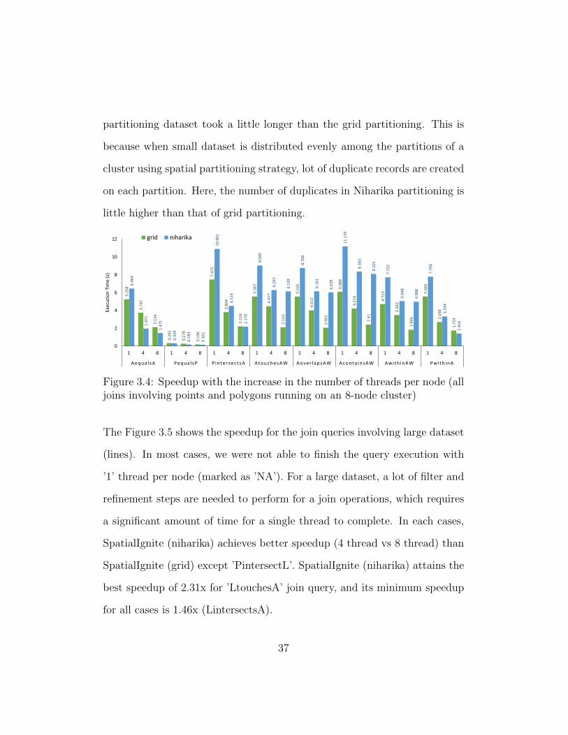
partitioning dataset took a little longer than the grid partitioning. This is
because when small dataset is distributed evenly among the partitions of a
cluster using spatial partitioning strategy, lot of duplicate records are created
on each partition. Here, the number of duplicates in Niharika partitioning is
little higher than that of grid partitioning.
5.2
58
3.7
47
2.1
34
0.3
45
0.2
78
0.1
96
7.4
75
3.8
04
2.2
24
5.5
67
4.4
77
2.1
14
5.5
56
4.0
13
2.0
62
6.0
88
4.2
14
2.4
1
4.7
13
3.4
92
1.8
46
5.5
65
2.6
98
1.7
54
6.4
64
1.9
71
1.4
71
0.3
29
0.1
83
0.1
61
10
.90
1
4.5
14
2.1
79
9.0
45
6.2
97
6.1
39
8.7
68
6.1
61
6.0
39
11
.17
9
8.3
63
8.1
01
7.7
22
5.0
48
4.9
88
7.7
94
3.3
34
1.4
16
0
2
4
6
8
10
12
1 4 8 1 4 8 1 4 8 1 4 8 1 4 8 1 4 8 1 4 8 1 4 8
AequalsA PequalsP P intersectsA Ato uchesAW Ao v er lapsAW Aco nta insAW Awith inAW Pwith inA
Exec
uti
on
Tim
e (s
)
grid niharika
Figure 3.4: Speedup with the increase in the number of threads per node (alljoins involving points and polygons running on an 8-node cluster)
The Figure 3.5 shows the speedup for the join queries involving large dataset
(lines). In most cases, we were not able to finish the query execution with
’1’ thread per node (marked as ’NA’). For a large dataset, a lot of filter and
refinement steps are needed to perform for a join operations, which requires
a significant amount of time for a single thread to complete. In each cases,
SpatialIgnite (niharika) achieves better speedup (4 thread vs 8 thread) than
SpatialIgnite (grid) except ’PintersectL’. SpatialIgnite (niharika) attains the
best speedup of 2.31x for ’LtouchesA’ join query, and its minimum speedup
for all cases is 1.46x (LintersectsA).
37

0.8
83
0.6
53
0.3
28
16
9.1
11
16
1.2
16
2.3
62
16
1.8
91
12
6.0
51
12
5.4
89 15
7.8
67
15
2.2
69
98
.33
1
59
.15
5
1.0
43
0.4
23
0.5
97
18
7.0
22
12
7.5
04
22
4.6
08
96
.91
2
11
7.6
04
60
.44
3
14
8.0
83
72
.11
9
26
0.8
62
87
.84
2
49
.91
1
0
50
100
150
200
250
300
1 4 8 1 4 8 1 4 8 1 4 8 1 4 8 1 4 8
PintersectsL L intersectsA LtouchesA Lwith inA LcrossesA LcrossesL
Exec
uti
on
Tim
e (s
)
grid niharika
NA
NA
NA
NA
NA
NA
NA
NA
NA
Figure 3.5: Speedup with the increase in the number of threads per node (alljoins involving lines running on an 8-node cluster)
Spatial Join We have evaluated 14 types of pairwise spatial join queries
listed in the Table 3.2. In case of SpatialIgnite, we have considered the exe-
cution time with eight threads per node. If we look at Figure 3.6, SpatialIg-
nite (grid) performs better than SpatailIgnite (niharika) for joining smaller
datasets (e.g., pointlm, arealm and areawater). However, SpatialIgnite (ni-
harika) performs better with join operations invloving large dataset (lines).
This is because some partitions in a grid partitioning scheme contain a lot of
data objects which takes much time to process. Also, it is faster to aggregate
small return result.
Spatial Analysis: Figure 3.7 shows the average execution time of 10 spatial
analysis operations involving point, line and polygon dataset. As spatial
analysis functions are not compute-intensive, time to execute these functions
is not significantly different in both partitioning. In most cases, when the
dataset is small (points and polygons), SpatialIgnite (grid) performs better
than SpatialIgnie (niharika). However, as we mentioned before, SpatialIgnite
38

0.01
0.1
1
10
100
Exec
uti
on
Tim
e (
s) -
logs
cale
SpatialIgnite(grid) SpatialIgnite(niharika)
Figure 3.6: Spatial Join involving Points, Lines and Polygons (on an 8-nodecluster)
(niharika) performs better with a large dataset (lines).
0.001
0.01
0.1
1
10
Exec
uti
on
Tim
e (s
) -
logs
cale
SpatialIgnite(gird) SpatialIgnite(niharika)
Figure 3.7: Spatial Analysis queries involving Points, Lines and Polygons (onan 8-node cluster)
Range Query: We evaluate the range queries involving point, line and
polygon datasets for a given query window (see Figure 3.8). As like be-
fore, SpatialIgnite (grid) perform better with the smaller dataset (pointlm,
arealm, and areawater), however, SpatialIgnite(niharika) perform better for
line range queries.
39

0.001
0.01
0.1
1
10
RangeQuery(Point) RangeQuery(Area) RangeQuery(AreaWater) RangeQuery(Line)
Exe
cuti
on
Tim
e (s
) -
logs
cale
SpatialIgnite(grid) SpatialIgnite(niharika)
Figure 3.8: Range queries involving Points, Lines and Polygons (on an 8-nodecluster)
3.7 Summary
In this chapter, we introduced SpatialIgnite with two spatial data parti-
tioning techniques and important spatial-join and analysis features. The
performance of SpatialIgnite is evaluated with a different number of threads
using several workloads. We believe that efficient distributed SQL and rich
set of OGC [27] compliant spatial join and analysis features will alleviate the
lack of present Hadoop and Spark based big spatial data systems.
40

Chapter 4
Benchmarking Big Spatial Data
Processing Systems
4.1 Introduction
A significant portion of today’s big data is big spatial data and these data
comes from diverse sources in various formats. Also, a wide range of applica-
tions and services directly depend on the processing of spatial data. There-
fore, researchers around the world have been involved in projects to meet the
demands for spatial data processing systems. A number of big spatial data
systems emerged in recent years. Also, these systems vary widely in terms
of available features, support for geometry data types and query categories,
indexing techniques, data partitioning techniques, and spatial analysis func-
tionalities. Therefore, it is essential to know the current state of big spatial
41
data systems. It is also essential to understand the key factors of evaluating
a new system. Benchmarking is generally considered as a process of evalu-
ating a system against some reference to measure the relative performance
of the system [6]. A few previous projects have discussed some factors of
benchmarking while evaluating big spatial data systems. However, as far as
we know, none of these projects conducted a comprehensive study on big
spatial data systems.
We have proposed a benchmark [3] for evaluating big spatial data processing
systems which is inspired by a micro benchmark of Jackpine [33]. The pur-
pose of this benchmark is to compare the SpatialIgnite with other systems,
on one hand, and is to use this benchmark independently for evaluating any
big spatial data systems, on the other hand. We believe that this bench-
mark will help the stakeholders of big spatial data systems in many ways for
furthering state of the art as below:
• provides a complete picture of the current state of Hadoop and Spark
based big spatial data systems.
• discusses various performance evaluation factors such as execution time,
scalability, and speedup.
• provides a idea of integrating new features to improve the performance
of spatial data systems.
• explains the importance of spatial analysis functions in future big spa-
tial data systems.
42

Parts of this chapter have been published in [3]. The rest of the chapter is
organized as follows. In Section 4.2, we review the previous work related to
benchmarking big spatial data systems. We present a comparative analysis
of existing big spatial data systems in Sections 4.3, and 4.4. We describe the
benchmark workload in Section 4.5. We present the performance evaluation
in Section 4.6. Finally, we conclude the chapter in Section 4.7.
4.2 Related Work
Benchmark play an important role in evaluating the functionality and per-
formance of a particular system against a reference system. The Transac-
tion Processing Performance Council (TPC) [45] is an organization that has
developed several database related benchmarks. Among them, TPC-C (an
On-line Transaction Processing benchmark), and TPC-H (a decision support
benchmark) are the most widely used. However, TPC does not have any spa-
tial benchmark. Perhaps the earliest known benchmark for spatial databases
is SEQUOIA 2000 [39], which focused on raster data based on Earth sci-
ences. Subsequently, OGC played an important role in standardizing spatial
topological relations and spatial functions. Jackpine [33] is a popular spatial
database benchmark that incorporates a comprehensive workload based on
OGC standards as part of its micro benchmark. It also includes a number
of real-world applications in its macro benchmark suite. Jackpine was pri-
marily developed to evaluate relational databases with support for spatial
43
functionalities.
Due to the rapid rise in spatial data volume, a number of Big Spatial Data
systems have emerged in recent times. It has been demonstrated in [36] that
spatial data processing has significantly different characteristics than regular
data processing. Therefore, understanding the performance characteristics of
these systems is of great interest to many stakeholders and researchers. How-
ever, there have been only a few projects (discussed below) that evaluated
isolated spatial operations.
Francisco et al. [11] performed a comparative analysis of disk-based spa-
tial data system SpatialHadoop [1] and Spark-based in-memory spatial data
system LocationSpark [41]. Their main focus was only Distance Join queries.
Their analysis shows that LocationSpark performs better than SpatialHadoop
in terms of execution time, but SpatialHadoop is a more mature system.
Stefan et al. [18] also analyzed the features and performance of Hadoop and
Spark-based Big Spatial data processing systems. They evaluated the perfor-
mance of their system STARK [19] with SpatialSpark [48], GeoSpark [49] and
SpatialHadoop [1] for range queries and a spatial join operation (involving
two point datasets and Equal predicate).
Rakesh et al. [24] discussed the architectural comparison of two spatial big
data systems SpatialHadoop [1] and GeoSpark [49], where they show that
GeoSpark is faster in processing spatial data than SpatialHadoop.
As indexing is one of the most important aspects of spatial data processing,
George et al. [34] have done a performance study on Quadtree-based index
44

structure xBR+-tree and R-tree based index structure R*-tree and R+-tree in
the context of most common spatial queries, such as point location, window,
distance range, nearest-neighbor, and distance-based join. They evaluate the
performance based on I/O efficiency and execution time on point dataset and
the result shows that the performance of xBR+-tree is better than R*-tree
and R+-tree in most cases.
None of the above-mentioned projects conducted a comprehensive perfor-
mance study of Big Spatial Data systems based on the OGC standards.
Hence, there is a great need for such a benchmark that can help the research
community for assessing how to take their research to the next level. Our
benchmark is intended to fill this void and is inspired by Jackpine. To our
knowledge, this is the first comprehensive study of Big Spatial Data systems.
In Sections 4.3 and 4.4, we provide a detailed background and feature analysis
of Hadoop-based Big Spatial Data systems and distributed in-memory Big
Spatial Data systems.
4.3 Hadoop-based Big Spatial Data Systems
As Hadoop [17, 35] became a popular framework to process big data in both
research community and industry, a number of extensions to Hadoop were
proposed. Distributed Big spatial data systems like SpatialHadoop [38] and
Hadoop-GIS [2] were developed by extending Hadoop and MapReduce frame-
work. A detailed feature matrix of these systems is presented in Table 4.1.
45

Hadoop-GIS [2] is a spatial extension of Hadoop to process large-scale spatial
data using MapReduce framework. First, it declusters the data and stores it
into HDFS. Then it adds a global index to each tile, which is stored in HDFS
and shared across the cluster nodes. Its query engine RESQUE can index the
data locally on the fly if required, which is stored in memory for faster query
processing. Initially, it supported Hilbert Tree and R*-tree for global and
local data indexing. Later, SATO [46] was introduced, which is a spatial data
partitioning framework integrated with Hadoop-GIS. SATO supports several
partitioning and indexing strategies, such as fixed-grid, binary-split, Hilbert-
curve, strip, optimized strip, and STR. It can choose an optimal strategy
during spatial data processing. Finally, it integrates Hive [43] and extends the
HiveQL to support declarative spatial query language. The main issue with
Hadoop-GIS is that it is added as a layer on top of Hadoop without changing
its system core. As a result, its performance is not improved significantly.
In addition, Hadoop-GIS extends Hive for declarative spatial query support,
which adds an extra layer of overhead over Hadoop to process spatial queries.
SpatialHadoop [38] is a framework, which incorporates spatial data process-
ing support in different layers of Hadoop, namely, Storage, MapReduce, Op-
erations, and Language layers. In the storage layer, SpatialHadoop added
a two-level index structure called global and local index. The global in-
dex is created for each data partition across the cluster and the local index
organizes the data inside each node. Thus, during a query operation, Spa-
tialHadoop can utilize the information regarding which partition is mapped
46

Table 4.1: Hadoop-based Big Spatial Data Systems
Features SpatialHadoop Hadoop-GISgeometry type point, line, polygon point, line, polygoninput-format WKT WKT
query language PigeonHiveQL
with spatial support
partitioning& indexing
grid, R-tree(STR), R+-tree
SATO(fixed-grid, binary-split,
hilbert-curve, strip,optimized strip,
STR)
spatial operationrange query, kNN,
spatial-join,distance-join
range, kNN,spatial-join
query planing &optimization
partition andquery skew
partition andquery skew
spatial analytics convexhull, skyline notemporal feature no no
to which node and which block of that node is relevant. This can make
the query processing faster. In addition, steps are taken during partitioning
to reduce the partition and query skew. It introduces two components in
the MapReduce layer, namely, SpatialFIleSplitter and SpatialRecordReader.
SpatialFIleSplitter utilizes the global index to split the input into files and
SpatialRecordReader extracts the records from each split by utilizing local
index and passing them to the map function. Spatial operations such as
range queries, kNN queries, and spatial join query over geometric objects
implemented as MapReduce programs in the Operation layer. An OGC-
compliant [27] high-level language Pigeon [8] is added to the language layer.
Pigeon is an extension of Pig [30, 28], which includes support for geometry
47

data type, spatial predicates, and various spatial operators to run a spatial
query on SpatialHadoop. However, it is not efficient to perform join oper-
ations with Pigeon, because it uses the cross product operation for joining,
which is very costly. Otherwise, since SpatialHadoop modified the system
core of Hadoop, it overcomes some of the limitations of Hadoop-GIS and
improves the spatial query performance significantly.
4.4 Distributed In-Memory Big Spatial Data
Systems
In this section, we describe two categories of distributed in-memory big spa-
tial data systems: Spark-based distributed in-memory systems and other
distributed in-memory systems.
4.4.1 Spark-based Big Spatial Data Systems
Currently, Apache Spark [37, 52] is widely used distributed in-memory sys-
tem for big data processing. It can reduce the execution time significantly
compared to MapReduce jobs on Hadoop [17, 35]. However, Spark does not
have any support for processing spatial data. It processes spatial data by
treating it as a non-spatial data due to the lack of spatial indexing, spatial
data skew handling and spatial query optimization [41]. To alleviate these
limitations, several Spark-based spatial data analysis systems have been pro-
48

posed in the last few years. A detailed feature matrix of these systems is
presented in Table 4.2.
Table 4.2: Spark-based Big Spatial Data Systems
Features SpatialSpark GeoSpark Simba LocationSpark STARK
geometry typepoint, line,
polygonpoint, line,
polygonpoint
point, line,polygon
geometry
input-format WKTCSV, TSV, WKT,WKB, GeoJSON,
Shapefile
CSV, JSON,Parquet
WKT WKT, Time
query language no SQL(2017) SQL no Piglet
partitioningFixed-Grid,Binary-Split,
Sort-Tile
R-tree,voronoi diagram,
Quad-treeSTR
Grid,region Quadtree
Fixed Grid,Cost-based
Binary Split
indexing R-tree R-tree, Quad-tree R-treeR-tree, Quadtree,
IR-tree)R-tree
(live, persistent)
spatialoperation
range query,broadcast-join,partitioned-join
range query,kNN query,spatial-join,distance-join
range query,kNN query,
distance-join,kNN-join
range search,range join
kNN Search,kNN-join
kNN query,spatial-join
optimization no nopartition skew,
query-skew
partition skew,query-skew,
communication costpartition skew
memorymanagement
no no no yes no
spatialanalytics
no no noclustering, skyline,
spatio-textualtopic summarization
clustering
temporalfeature
no no no no yes
GeoSpark [49] is an in-memory cluster computing framework for processing
large-scale spatial data. It adds an extension to Apache Spark to support
spatial data types and operations. It introduces four different types of Spa-
tial RDDs (SRDDs) based on Spark RDDs [50], namely, PointRDD, Rect-
angleRDD, PolygonRDD and LineStringRDD. It efficiently partitions the
SRDD data elements across cluster nodes using Quad-Tree, R-Tree, Voronoi
diagram and Fixed-Grid. It uses Quad-Tree and R-Tree indexing techniques
to index data on each node. It executes spatial queries such as range query,
49

kNN query, and join query on big spatial datasets by extending the SRDD
layer. The system core of GeoSpark mainly consists of three layers. The
Spark Layer performs basic Spark operations like data loading into a disk,
Spatial RDD Layer provides geometrical and spatial object support to Spark
RDD, and finally, Spatial Query Processing Layer performs the spatial query
on Spatial RDD. The main limitation of GeoSpark is that it is developed as
a library on top of Spark, not as a part of Spark-core, which is not efficient
in order to execute spatial queries. Although initially it did not support
SQL queries, recently GeoSpark SQL [21] has been introduced. In addition,
GeoSpark does not have any support for handling data and query skew.
SpatialSpark [48] implements several spatial operations on Spark to analyze
large-scale spatial data. It supports two spatial join operations, where broad-
cast join is used to join a big data set with a smaller dataset and partition
join is used to join two big dataset. It can perform spatial range query with-
/without index. These operations can be performed over geometric objects
using spatial predicates: intersect, within, overlap, contains, within distance
or nearest distance. Data can be partitioned using Fixed-Grid, Binary-Split,
and Sort-Tile partitioning techniques and indexing using R-tree. However,
like GeoSpark, it also implemented the spatial support on top of Spark with-
out modifying Spark core. To our knowledge, there is no plan by the Spa-
tialSpark developers to handle data skew and query optimization.
LocationSpark [41] is an efficient spatial data processing system developed
based on Apache Spark. It stores spatial data as a key-value pair, where the
50
key can be any geometry data type such as point, a line-segment, a poly-
line, a rectangle, or a polygon and the value type can be specified by the
user as a text. It supports a wide range of spatial queries including spatial
range-search, range-join, kNN-search, and kNN-join query. It also supports
few spatial analysis functions, such as spatial data clustering, spatial skyline
computation, and spatio-textual topic summarization. The query scheduler of
LocationSpark contains an efficient cost model and a query execution plan to
mitigate and deal with two types of skew: (1) data partitioning skew and (2)
query skew. Its global index (grid and region Quadtree) partitions the data
among various nodes and a local index (an R-tree, a variant of the Quadtree,
or an IR-tree) used to index data on each node. Also, LocationSpark added
a spatial bloom filter to reduce the communication cost of the global spatial
index, which can answer whether a spatial point is contained inside a spatial
range. Finally, to efficiently manage main memory, it dynamically caches
frequently accessed data into memory, and stores less frequently used data
into the disk, reducing the number of I/O operations significantly. It can be
used as a library on top of Apache Spark. However, it does not have any
spatial query language support like SQL.
Simba [47] is a distributed in-memory analytics engine for spatial data pro-
cessing, which is developed by extending SparkSQL [5] and DataFrame API.
The extension of DataFrame API opens the possibility for Simba to interact
with other important Spark tools such as MLlib, GraphX etc. It partitions
the data using STR partitioner by considering partition size, data locality
51
and load balancing. Like LocationSpark, it also adopts a two level index-
ing (R-tree) scheme, where the global index helps to prune the irrelevant
partitions for a query and local index accelerates the query processing in
each partition. Currently, it supports spatial operations over point and rect-
angle objects, including range query, kNN query, spatial distance, and kNN
join. Moreover, its spatial-aware and cost-based optimization to select a good
query plan helps to achieve both low latency and high throughput. But it
only support points, and hence, it is not possible to perform spatial join over
geometric objects, such as, polygon or line with Simba. The experimental
results show that Simba outperforms SpatialSpark and GeoSpark on point
based operations.
STARK [19] is a spatio-temporal data processing framework which is tightly
integrated with Spark in order to support spatial data types and operators.
Currently, STARK supports two types of spatial partitioning. The fixed grid
partitioner applies a grid over the data space, where each grid cell corre-
sponds to one partition. The cost-based binary split partitioner generates
partition based on the number of contained elements. STARK allows two
modes for indexing, where live index is built upon execution for each par-
tition, queried according to the current predicate (contains/intersects), and
then thrown away. And the persistent indexing allows to create the index and
write the indexed RDD to disk or HDFS. This stored index can be loaded
again to save the cost of generating it. But it can run a query on both in-
dexed as well as unindexed data. STARK also extended the Pig Latin, called
52

Piglet, to support declarative query language for spatial data processing. In
Piglet, STARK introduced geometry data type and added spatial operators
for spatial predicates, join and indexing. Based on the information avail-
able, among the Spark-based spatial data systems, only STARK supports
temporal feature, but no evaluation of that feature has been reported.
4.4.2 Other Distributed In-memory Big Spatial Data
Systems
Apache Ignite [22] is an open source distributed in-memory big data pro-
cessing platform, which supports many features of big data systems as well
as some features of relational DBMS. Caching and parallel query processing
on in-memory data are two important features that contribute to its good
performance. First, it keeps data in a cache in the main memory data grid
distributed across a cluster of nodes and it is horizontally scalable. Second,
it performs parallel processing of queries on data in the cache. However,
Ignite’s support for spatial features is rather limited. Currently, it has sup-
port for geometry data types (point, line, and polygon) and a limited form
of querying on geometry objects.
We introduce SpatialIgnite, which is an extension of Apache Ignite. The
spatial join and spatial analysis support of SpatialIgnite are implemented
using the JTS library [23]. In this study, we evaluate the performance of
SpatialIgnite with two other existing big spatial data systems. The main
53

Table 4.3: Features of SpatialIgnite
Features SpatialIgnitegeometry type point, line, polygoninput format WKT
query language Distributed SQLpartitioning grid, Niharika[32] + Rendezvous Hashing
indexing R-treequery planning,
optimizationyes
spatial operationspatial-join (supports all
OGC-compliant join predicates),range query
spatial analytics all (see Table 4.5)temporal feature no
Table 4.4: Existing Support of Spatial Join Predicates
JoinPredicates
SpatialHadoop GeoSpark SpatialIgnite
Equals N N YIntersects Y Y YTouches N N YOverlaps Y N YContains N Y YCrosses N N Y
features of SpatialIgnite is illustrated in Table 4.3.
4.5 Our Benchmark
As mentioned earlier, the goal is to conduct a comprehensive evaluation
of Big Spatial Data systems. This benchmark is inspired by Jackpine [33]
micro benchmark, and it includes various spatial join operations with OGC-
54

Table 4.5: Existing Support of Spatial Analysis Functions
SpatialAnalysis
SpatialHadoop GeoSpark SpatialIgnite
Distance N N YWithin N N Y
Dimension N N YEnvelope N N YLength N N YArea N N Y
Buffer N N YConvexHull Y N Y
compliant topological predicates and spatial analysis functions. However,
most of the big spatial data systems do not support all of these features.
The existing spatial join predicates and analysis functions supported by Spa-
tialHadoop, and GeoSpark are shown in Tables 4.4 and 4.5, where ’Y’ means
a feature is supported and ’N’ means it is not supported. Also, these two
tables give the features supported by our SpatialIgnite system.
4.5.1 Workload
The workload of a benchmark is comprised of spatial join operations, range
queries and spatial analysis functions. The complete list of the operations in
our benchmark are shown in Table 3.2. We adopted these operations from
Jackpine and made some changes (marked with ’*’), which are listed in the
table. Specifically, in Jackpine benchmark, some pair-wise join operations
involving line dataset did not use the whole line dataset (e.g. LineCrosses-
Line). They were changed to use the entire line dataset. Also, some pair-wise
55

join operations involving polygons contained a self-join in Jackpine, such as
the join operation ’PolygonOverlapsPolygon’ involved the arealm dataset.
These were changed into a join operation with two different datasets, for
example, ’ArealmOverlapsAreaWater’. Also, we added range queries in our
benchmark, which were not part of Jackpine.
4.5.2 Datasets
Our benchmark utilizes real-world spatial datasets which were obtained from
Tiger [44] (2011 release). These datasets consist of points, lines, and polygons
of California, USA. We have used four datasets from Tiger, including arealm
(polygon), areawater (polygon), pointlm (point) and edges (line). The details
of these datasets are given in Table 3.3.
4.6 Performance Evaluation
For the evaluation of Big Spatial Data systems, we consider three systems,
one from each category of the big spatial data systems. First, we choose a
Hadoop-based system SpatialHadoop [1, 38] as it is a mature system and its
performance is better than any other systems developed on Hadoop. Second,
we include Spark-based in-memory system GeoSpark [49], as it is one of the
most active projects (latest version v1.1.3 published on 26th April 2018) [13].
Also, it is mentioned as a Spark-based third-party infrastructure project.
Finally, we select SpatialIgnite, which we have proposed.
56

4.6.1 Benchmark Implementation
SpatialHadoop [1, 38] implemented the SJMR (Spatial Join with MapRe-
duce) algorithm in the core of SpatialHadoop using spatial predicate inter-
sect/overlap to perform the spatial join operation. It does not implement all
the OGC-compliant [27] join predicates inside the core of SpatialHadoop (see
Table 4.4). But they implemented the join predicates as part of a Pigeon [8],
which is added into the language layer of Hadoop. However, Pigeon performs
join operation through a cross product, which is very costly operation. From
our experience, even to perform a join operation like PointIntersectArea on a
small dataset, pointlm and arealm take almost 4 hours, whereas it takes only
25 seconds (approx.) if we run the same query from SpatialHadoop command
line (see Figure 4.1). We implemented all the spatial join predicates based-on
SJMR algorithm. All spatial join queries run using our implemented spatial
join predicates in this study.
Similarly, GeoSpark [49, 13] also implemented the spatial join queries using
contains/intersects predicates and it can run join queries with or without
using index (see Table 4.4). We implemented other spatial join predicates
on GeoSpark and changed the GeoSpark core accordingly to run the spatial
join queries.
Finally, we implemented the spatial join and analysis function supports on
Apache Ignite using JTS library [23] called SpatialIgnite. Along with Ignite’s
default partitioning (hash), we have introduced and evaluated two spatial
partitioning techniques (grid, and Niharika [32]) in SpatialIgnite.
57

4.6.2 Experimental Setup
The experiments were conducted on a cluster of 8 machines, each having an
Intel(R) Xeon(R) CPU E5472 @ 3.00GHz× 2 with 4× 2 cores, 16GB RAM,
and 500GB HDD running on Ubuntu 14.04 64-bit operating system with
Oracle JDK 1.8.0 81. Along with Hadoop-2.3.0, Spark-2.1.1 and Apache-
Ignite-Fabric-2.6.0 used in this evaluation.
4.6.3 Result Analysis and Discussion
We evaluated three categories of operations, as outlined in Table 3.2, for
performance evaluation. They include pair-wise spatial join, spatial analysis,
and range queries. The execution time of a query in each case is reported
based on the average elapsed time calculated over several runs. In each
case, we have compared the performance of SpatialIgnite (with different
partitioning schemes: hash, grid, and Niharika [32]) with SpatialHadoop and
GeoSpark. In each case of SpatialIgnite, we have used 8 threads per node.
As the default partitioning (hash) of SpatialIgnite does not consider the
spatial attribute to partition the dataset, its spatial join results are inaccu-
rate. Also, we have discovered that in all cases, GeoSpark returns inaccurate
results. We have illustrated the verification of the accuracy of results in
Table 4.6. We have used PostgreSQL/PostGIS as a reference system. If we
look at Table 4.6, the results of a query based on Ignite’s default partitioning
(hash) and GeoSpark are far different from PostgreSQL/PostGIS.
58

Table 4.6: Verification of Result Accuracy
PostgreSQL/PostGIS
SpatialIgnite(hash)
SpatialIgnite(grid)
SpatialIgnite(niharika)
GeoSpark SpatialHadoop
Point Intersects Area 1857 51 1592 1879 572 1859Point Intersects Line 39776 1368 40470 41191 NA 29489Line Intersects Area 206879 6767 171806 188604 5942 215750Area Touches AreaWater 908 35 937 1099 537 913Line Touches Area 86962 3762 107346 126502 5942 118353Area Overlaps AreaWater 224 9 224 288 170 227Area Contains AreaWater 3301 110 2224 3370 288 3305
• Spatial Join: We ran 14 types of pairwise spatial join queries involv-
ing point, line, and polygon on SpatialHadoop, GeoSpark, and SpatialIgnite
(hash, gird, and Niharika [32]). In case of GeoSpark, we were not able to
run some queries (marked as ’NA’ in Figure 4.1), because its execution en-
gine is designed in a way such that the query window is always a Polygon.
Thus, one dataset is always a polygon during the join operation. If we look
at Figure 4.1, in each case, GeoSpark and SpatialIgnite outperform Spa-
tialHadoop in terms of execution time. We mentioned that GeoSpark and
SpatialIgnite (hash) both returns inaccurate result. Also, the performance of
SpatialIgnite (Niharika) is better than SpatialIgnite (grid) for large datasets,
such as the queries that involve lines (edges) in Table 3.2. Figure 4.1 shows
that SpatialIgnite (Niharika) does better than GeoSpark in all cases, except
for the query ’LineWithinArea’ and ’AreaContainsWaterArea’. Overall, the
performance of SpatialIgnite is better than the other systems.
• Spatial Analysis Queries: SpatialIgnite supports all of the spatial anal-
ysis functions in Table 3.2. However, SpatialHadoop only supports Convex-
Hull of points. GeoSpark does not have any support for the spatial analysis
59

0.01
0.1
1
10
100
Exec
uti
on
Tim
e (s
) -
logs
cale
SpatialHadoop GeoSpark SpatialIgnite(grid) SpatialIgnite(niharika) SpatialIgnite(hash)
NA
NA
NA
Figure 4.1: Spatial Join involving Points, Lines and Polygons (on an 8-nodecluster)
functions. Figure 4.2 shows the average execution time of 10 spatial analy-
sis operations involving point, line and polygon dataset. As spatial analysis
functions are not long-running, time to execute these functions is not signif-
icantly different among the systems. The time to construct the convex hull
of all points is almost the same in both SpatialHadoop and SpatialIgnite.
0.001
0.01
0.1
1
10
Exec
uti
on
Tim
e (s
) -
logs
cale
SpatialHadoop GeoSpark SpatialIgnite(gird) SpatialIgnite(niharika) SpatialIgnite(hash)
NA
NA
NA
NA
NA
NA
NA
NA
NA
NA
NA
NA
NA
NA
NA
NA
NA
Figure 4.2: Spatial Analysis queries involving Points, Lines and Polygons (onan 8-node cluster)
60

• Range Query: We ran the range queries (in Table 3.2) involving point,
line and polygon datasets for a given query window. The performance of
GeoSpark and SpatialHadoop is not significantly different in all cases, except
for the range queries in the polygon (arealm) dataset, where SpatialHadoop
performs better. In all cases, SpatialIgnite (hash, grid, and Niharika [32])
performs better than the SpatialHadoop and GeoSpark. However, for line
range queries, execution time is almost similar among all the systems.
0.001
0.01
0.1
1
10
100
RangeQuery(Point) RangeQuery(Area) RangeQuery(AreaWater) RangeQuery(Line)
Exec
uti
on
Tim
e (s
) -
logs
cale
SpatialHadoop GeoSpark SpatialIgnite(grid) SpatialIgnite(niharika) SpatialIgnite(hash)
Figure 4.3: Range queries involving Points, Lines and Polygons (on an 8-nodecluster)
• Scalability with increase in number of nodes:
We have investigated the scalability of the evaluated systems by varying
the number of nodes to 4 and 8. We only consider compute-intensive join
queries involving the large dataset (lines). If we look at Figure 4.4, Spatial-
Hadoop performs well with a 4-node cluster. As it is a disk-based system, the
I/O overhead increases with the increase in the number of nodes. Also, the
polygon datasets (arealm and areawater) are not large enough to make an
impact on the performance with the increased number of nodes in disk-based
61

systems. The performance of GeoSpark is better than SpatialIgntie (grid)
in both 4-node and 8-node settings. However, Geospark returns inaccurate
results. SpatialIgnite (Niharika) performs better than GeoSpark when we
increase the number of node in all cases except ’LineWithinArea’. SpatialIg-
nite (Niharika) attains the best speedup of 1.66x for ’LineTouchesArea’ join
query, and its minimum speedup for all cases is 1.38x (LineWithinArea).
37
7.0
02
49
7.4
89
14
0.6
34
13
3.5
36
18
9.4
89
16
1.2 19
0.6
15
12
7.5
04
14
9.6
85
77
.76
37
6.9
15
48
5.1
79
13
8.3
61
12
3.9
37 19
3.4
11
16
1.8
91
16
1.4
89
96
.91
2
13
2.0
57
70
.32
4
37
7.5
89
49
2.9
05
58
.33
8
37
.17
2
13
6.6
38
12
5.4
89
83
.79
5
60
.44
3
10
1.3
23
54
.91
7
37
6.4
75
48
4.6
06
14
0.8
25
12
5.6
13
16
7.3
15
2.2
69
10
3.9
77
72
.11
9 12
7.3
23
68
.55
3
0
100
200
300
400
500
600
4 - N o d e 8 - N o d e 4 - N o d e 8 - N o d e 4 - N o d e 8 - N o d e 4 - N o d e 8 - N o d e 4 - N o d e 8 - N o d e
S p a t i a l H a d o o p G e o S p a r k S p a t i a l I g n i t e ( g r i d ) S p a t i a l I g n i t e ( n i h a r i k a ) S p a t i a l I g n i t e ( h a s h )
Exe
cuti
on
TIm
e (
s)
LineIntersectsArea LineTouchesArea LineWithinArea LineCrossesArea
Figure 4.4: Performance Comparison - Scalability (4-nodes vs 8 nodes)
4.7 Summary
This chapter presented our proposed big spatial data systems benchmark [3]
by providing detailed information about the current state of big spatial data
systems. The important factors for evaluating a big spatial data system are
also presented. We have evaluated three systems based on execution time,
speedup, and scalability. The evaluation shows that the result returned from
GeoSpark and SpatialIgnite (hash) are inaccurate. However, we addressed
62

the issue of inaccurate result of SpatialIgnite by introducing two spatial par-
titioning schemes: grid and Niharika [32]. We hope that this benchmark will
help the community in future research of big spatial data systems.
63

Chapter 5
Parallax: A Parallel Big Spatial
Database System
5.1 Introduction
The popular relational DBMS PostgreSQL, with spatial extension PostGIS,
is an efficient spatial data processing system in a single node environment.
However, due to the lack of parallelism, it is not efficient for processing
large-scale spatial data. Niharika [32] utilizes the powerful features of Post-
greSQL/PostGIS to implement a parallel query processing system along with
efficient data declustering and load balancing technique. However, as its stor-
age layer is not distributed, it needs to replicate the whole dataset in each
node. Also, as today’s spatial data comes from diverse sources in different
formats, it may not be always possible to store the data in a database table.
64

Furthermore, the ETL (extract, transform, and load) steps to import data
from a raw data source into a relational database can be expensive.
In this chapter, we introduce a parallel big spatial database system, called
Parallax. Parallax utilizes the power of PostgreSQL/PostGIS and Al-
luxio [25, 4] to process the large scale spatial data. Its host specific spatial
data partitioning, and intra-node query parallelism utilizes the main memory,
disk storage and processing cores of each node of a cluster.
The rest of the chapter is organized as follows. In Section 5.2, we illustrate
the architecture of Parallax. We discuss about PostgreSQL foreign data
wrapper library for Alluxio in Section 5.3. We explain data partitioning
and query execution process in Section 5.4 and Section 5.5 respectively. We
present the performance evaluation in Section 5.6. Finally, we conclude the
chapter in Section 5.7.
5.2 Architecture
The architecture of Parallax is illustrated in Figure 5.1. Parallax consists
of 3 layers: (1) Parallel Query Processing Layer (Coordinator), (2) Query
Execution Layer (PostgreSQL/PostGIS), and (3) Virtual Distributed Storage
Layer (Alluxio).
Parallel Query Processing Layer: This layer coordinates the parallel query
processing tasks from a master node by allocating query tasks to worker
nodes. Each worker node performs the task locally on a portion of the dataset
65

Coordinator
Alluxio
alluxio_fdw alluxio_fdw alluxio_fdw alluxio_fdw
Foreign Table Foreign Table Foreign Table Foreign Table
DB Worker
(PostgreSQL
+ PostGIS)
DB Worker
(PostgreSQL
+ PostGIS)
DB Worker
(PostgreSQL
+ PostGIS)
DB Worker
(PostgreSQL
+ PostGIS)
JDBC
SchedulerQuery
CustomizerResult
Aggregator
Spatial Data Declustering
PartitionAllocator
Query Processing
Layer
Query Execution
Layer
Distributed Storage
Layer
Figure 5.1: Architecture of Parallax
and returns the result to the master node. The coordinator also performs
aggregation, group-by operation, and duplicate elimination on/from the re-
sultset.
Query Execution Layer: This layer consists of worker nodes called DB-
Workers. Each DBWorker runs a standard PostgreSQL/PostGIS database
instance, each of which is connected with Alluxio through a foreign data
wrapper (alluxio fdw). Parallax creates foreign partition tables on each
database instance for a dataset resides in Alluxio storage. Each partition
table is connected to a respective chunk of that dataset in Alluxio storage
defined by alluxio fdw. Such dataset is reffered to foreign dataset. This
layer can execute query on foreign tables just like normal tables.
Virtual Distributed Storage Layer: We have integrated Alluxio [25] as
66

a virtual storage layer in Parallax. As the local file system of Alluxio is
distributed, we have used local storage (HDD) as persistence storage in
Parallax. Therefore, Alluxio keeps the hot data in main memory (RAM)
and the cold data in HDD. As the hot data always in the main memory,
Parallax experience much better I/O performance than directly interacting
with the persistent storage systems. We have used host specific location pol-
icy to distribute the data among the nodes of a cluster which ensures the
portion of data of same spatial boundary is in the same node.
5.3 PostgreSQL Foreign Data Wrapper for
Alluxio
A foreign data wrapper is a library in PostgreSQL to access data from exter-
nal sources, called foreign data. We have implemented foreign data wrapper
(alluxio fdw) for PostgreSQL to access data from Alluxio under storage sys-
tem. As Alluxio is written in Java and does not have any C/C++ API, we
also wrote a C wrapper for Alluxio and modified the PostgreSQL backend to
read/write data from/to Alluxio.
In PostgreSQL, a foreign server defines the connection of remote source,
and a foreign table defines the structure of the remote dataset. PostgreSQL
performs queries on remote source through a foreign table just like a nor-
mal table. However, the foreign table does not store any data in the table.
PostgreSQL either fetches or updates data from/to external source based on
67

remote data structure defined in the foreign table. A simple instruction to
install and use the Alluxio foreign data wrapper (alluxio fdw) with Post-
greSQL is listed below:
# cd /path/to/postgresql-9.6.4/contrib/alluxio_fdw/
# make
# make install
# psql mydb
mydb=# CREATE EXTENSION alluxio_fdw;
mydb=# CREATE SERVER alluxio_server FOREIGN DATA WRAPPER alluxio_fdw;
mydb=# CREATE FOREIGN TABLE ft_area(gid int, geom geometry)
SERVER alluxio_server
OPTIONS (format ’csv’, filename ’/arealm/arealm.csv’,
cpalluxio ’alluxio’, delimiter ’|’);
mydb=# CREATE FOREIGN TABLE ft_point(gid int, geom geometry)
SERVER alluxio_server
OPTIONS (format ’csv’, filename ’/pointlm/pointlm.csv’,
cpalluxio ’alluxio’, delimiter ’|’);
mydb=# SELECT COUNT(*)
FROM ft_point a, ft_area b
WHERE ST_Intersects(a.geom, b.geom);
68

5.4 Host Specific Spatial Data Partitioning
The regular grid partitioning approach is used to partition the dataset. In
grid partitioning, the whole spatial space is partitioned into equal-sized grids,
where each grid cell is a partition. We utilize the host specific location
policy (SpecificHostPolicy) of Alluxio to distribute the partitions across
the worker nodes of a cluster. This feature brings the following benefits into
Parallax:
• Ensure data partitions of the same spatial boundary is in the same
node.
• Ensure load balancing across the cluster. Therefore, Parallax able to
exploit the main memory, disk storage and CPU cores of each worker
node.
• As each data partition connects with foreign partition table of Post-
greSQL, Parallax can parallelize same the query in each worker node
on local data partitions.
In addition to the host specific location policy, Alluxio also supports the
following location policies:
• LocalFirstPolicy: Here, local host is the priority. If the local worker
does not have enough capacity of a block, then it randomly picks a
worker host from the active worker’s list. This is also the default policy
of Alluxio.
69

• MostAvailableFirstPolicy: This policy selects the worker with the most
available bytes.
• RoundRobinPolicy: It selects the worker for the next block in a round-
robin fashion and skips workers that do not have enough capacity.
5.5 Query Execution in Parallax
Parallax creates foreign partition tables in each instance of PostgreSQL/-
PostGIS across the cluster. Here each partition table connects with a re-
spective data partitions residing in that worker node through Alluxio foreign
data wrapper (alluxio fdw). During query execution, Parallax splits the
query across the cluster using the same way we distribute the data parti-
tions. As spatial data partitioning creates some empty partitions, Parallax
does not assign query related with empty partitions. Therefore, Parallax
does not need to check whether the partition is empty. Each worker node
executes the query on the respective data partition and returns the result to
the master node. Finally, the master node aggregates the result.
a1
a5
a9
a13
p1
p9
p13
p17
Node1, Dataset: arealm Node1, Dataset: pointlm
Figure 5.2: Spatial Join with Partitioned Dataset
70

When a dataset is partitioned using spatial partitioning approach, during a
join operation, only matching partitions of involving dataset (a1 of arealm
dataset with p1 of pointlm dataset) might have matching values[32]. There-
fore, joining a partition with other partitions of involving dataset (a5 of
arealm dataset with p9 of pointlm dataset) would not contribute to the re-
sultset. Therefore, Parallex query plan only executes a query on matching
partitions during spatial join operation which illustrated in the Figure. 5.2.
5.6 Performance Evaluation
Both Hadoop-based spatial data systems, SpatialHadoop [1] and Hadoop-
GIS [2], supports spatial query language. SpatialHadoop implemented Pi-
geon [8] as a spatial extension to Pig, and Hadoop-GIS added spatial support
with HiveQL [43]. As SpatialHadoop is a more mature system and Pigeon is
compliant with OGC [27], we choose Pigeon to evaluate with Parallax.
5.6.1 Experimental Setup
The experiments were conducted on a cluster of 4 machines, each having an
Intel(R) Core(TM) i5-2400 CPU @ 3.10GHz with 4 cores, 8GB RAM, and
500GB HDD running on Ubuntu 14.04 64-bit operating system with Oracle
JDK 1.8.0 121. Along with Hadoop-2.3.0, SpatialHadoop-2.4.2 with Pigeon-
0.2.2, PostgreSQL-9.6.4 with PostGIS-2.3.2 and Alluxio-1.2.0 was used in
this evaluation.
71
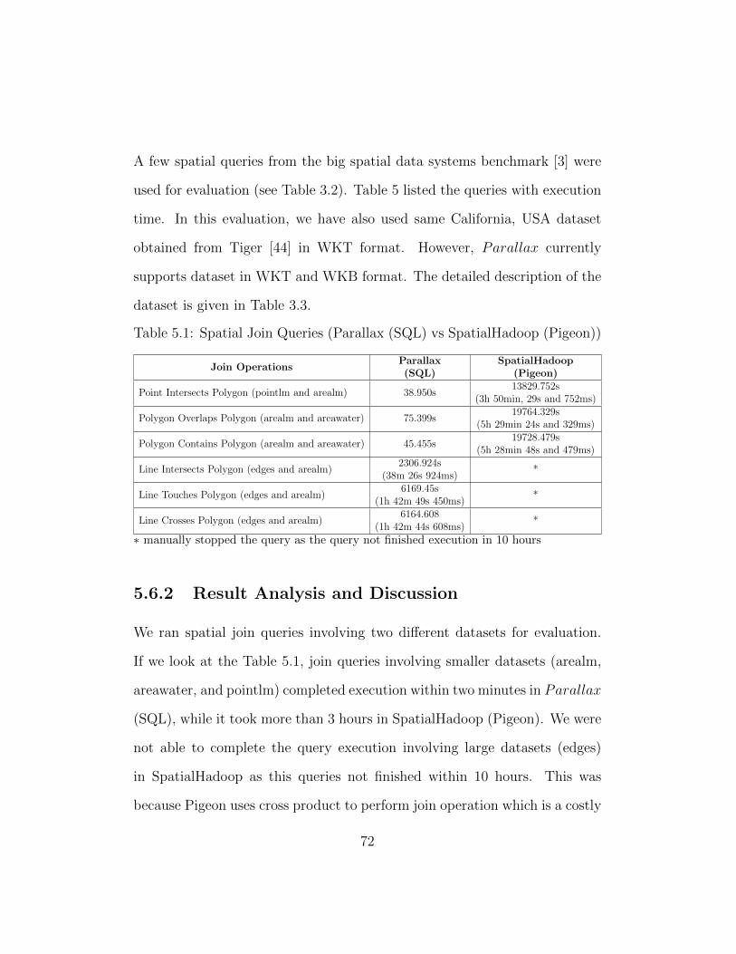
A few spatial queries from the big spatial data systems benchmark [3] were
used for evaluation (see Table 3.2). Table 5 listed the queries with execution
time. In this evaluation, we have also used same California, USA dataset
obtained from Tiger [44] in WKT format. However, Parallax currently
supports dataset in WKT and WKB format. The detailed description of the
dataset is given in Table 3.3.
Table 5.1: Spatial Join Queries (Parallax (SQL) vs SpatialHadoop (Pigeon))
Join OperationsParallax(SQL)
SpatialHadoop(Pigeon)
Point Intersects Polygon (pointlm and arealm) 38.950s13829.752s
(3h 50min, 29s and 752ms)
Polygon Overlaps Polygon (arealm and areawater) 75.399s19764.329s
(5h 29min 24s and 329ms)
Polygon Contains Polygon (arealm and areawater) 45.455s19728.479s
(5h 28min 48s and 479ms)
Line Intersects Polygon (edges and arealm)2306.924s
(38m 26s 924ms)*
Line Touches Polygon (edges and arealm)6169.45s
(1h 42m 49s 450ms)*
Line Crosses Polygon (edges and arealm)6164.608
(1h 42m 44s 608ms)*
∗ manually stopped the query as the query not finished execution in 10 hours
5.6.2 Result Analysis and Discussion
We ran spatial join queries involving two different datasets for evaluation.
If we look at the Table 5.1, join queries involving smaller datasets (arealm,
areawater, and pointlm) completed execution within two minutes in Parallax
(SQL), while it took more than 3 hours in SpatialHadoop (Pigeon). We were
not able to complete the query execution involving large datasets (edges)
in SpatialHadoop as this queries not finished within 10 hours. This was
because Pigeon uses cross product to perform join operation which is a costly
72

operation. Although Parallax performs better than SpatialHadoop in all
cases, we did not get the expected result from Parallax. We discuss the
main reasons behind the performance degradation in the next section.
However, in real life, most queries are spatial analysis or range queries like:
"List the names of all bookstores with ten miles of UNB"
"List all customers who live in Fredericton and its adjoining cities"
Therefore, we ran two queries on our dataset which are shown in Table 5.2.
In each case, query completed within 3 seconds.
Table 5.2: Example of real life query
QueryParallax (SQL)
Execution Time (s)Find all areas in arealm dataset that are within 1000 distance unitsfrom a given point
2.45
Find all areas in the arealm dataset within a given query window 2.822
5.6.3 Reasons of Performance Degradation
As Hadoop does not utilize the main memory during data processing, the
main limitation of Hadoop-based spatial data systems is disk I/O overhead.
Therefore, we incorporated a distributed virtual storage system Alluxio [25]
in Parallax. As Alluxio always keeps the hot data in main memory, we
thought it would significantly improve the performance during remote read-
/write operations. However, we did not get the expected result due to the
following reasons.
73

During processing a query, each time PostgreSQL needs to connect and load
the data from Alluxio in-memory cache, parse the records, convert into in-
ternal format and load into PostgreSQL in-memory cache. This also involves
a lot of read operation. Moreover, Alluxio does not have any native C/C++
API. We have used a C wrapper to perform read/write operation through
Java API which is added extra overhead with Parallax. These overheads
are behind the overall performance degradation. The possible solutions to
improve the performance of Parallax are discussed in 6.2.
5.7 Summary
This chapter introduced Parallax which integrates powerful features of Post-
greSQL/PostGIS and Alluxio. Host-specific data partitioning and parallel
query on local data in each node ensures the maximum utilization of main
memory, disk storage, and CPU. Although the performance of Parallax is
not quite impressive, its powerful spatial SQL query and Alluxio virtual stor-
age layer alleviate the limitations of Hadoop-based spatial data systems.
74

Chapter 6
Conclusions and Future Work
The rapid growth of spatial data and the popularity of location-based ser-
vices and applications are changing the perspective of spatial data processing
systems. Along with high-performance computer systems, we need efficient
parallel and distributed data systems to process large volume of spatial data.
Due to the popularity of distributed computing platforms, such as Hadoop
and Spark, people from academia and industry started adding spatial support
within this platforms. However, these spatial data systems are not mature
and still most of them do not have any efficient query language like SQL as
in relational database systems with spatial support (e.g. PostgreSQL/Post-
GIS). Also, their spatial data analysis features are limited. Moreover, there
are no projects which conducted a comprehensive study on big spatial data
systems till date. Therefore, we do not have the full picture of the current
state of big spatial data systems.
75

We have proposed a benchmark and conducted a comprehensive study of
big spatial data systems. We investigated all the features and performance
issues with these systems, which will help the community in future research
of spatial data systems. We also introduced two big spatial data processing
systems, Parallax and SpatialIgnite to alleviate the lack within the present
Hadoop and Spark based big spatial data systems. We achieved excellent
result with SpatialIgnite. However, we did not get the expected performance
with Parallax. Still, there is a scope to improve both of this systems. In the
next two sections, we will review the research contributions of this thesis, as
well as discuss directions for future research.
6.1 Thesis Contributions
The following are the main contributions of this thesis:
(1) SpatialIgnite: Extended Spatial Support for Apache Ignite (chapter 3)
• We extended the spatial support of Apache Ignite [22] by integrating
spatial joins with all OGC [27] compliant topological relations, range
queries, and various spatial analysis functions.
• As Ignite does not consider spatial features for data partitioning, Spa-
tialIgnite introduced two spatial data partitioning approach (regular
grid and Nihariaka [32]) to distribute the data across the cluster evenly.
• We also measured the performance of spatial partitioning techniques
76

(grid, Niharika [32]) introduced in SpatialIgnite by running spatial
join queries, range queries, and spatial analysis queries.
(2) Benchmarking Big Spatial Data Systems (chapter 4)
• We have introduced a big spatial data systems benchmark [3] by exten-
sively analyzing the features and functionalities of Hadoop and Spark
based big spatial data systems.
• As SpatialHadoop [1] and GeoSpark [49] do not support many of the
spatial join predicates in their current implementation, we have im-
plemented these features with these systems as part of the benchmark
evaluation. We have also included SpatialIgnite as one of the three
evaluated systems in the benchmark.
• This benchmark presented the key factors for evaluating a big spatial
data system. We also evaluated the performance of SpatialIgnite, Spa-
tialHadoop, and GeoSpark based on speedup, scalability and execution
time.
(3) Parallax: A Parallel Big Spatial Database System (chapter 5)
• We have implemented a PostgreSQL foreign data wrapper library for
Alluxio [4, 25] (alluxio fdw) and modified the PostgreSQL backend to
perform a query on remote data sources through Alluxio. As Alluxio
does not have any native C/C++ API, we also wrote a C wrapper,
77

Hence, PostgreSQL can execute a query on Alluxio under storage sys-
tems through alluxio fdw. Finally, we modified the parallel query
processing system Niharika [32] to perform a parallel spatial query on
remote data sources through PostgreSQL.
• The host-specific spatial data declustering distributes the dataset evenly
on each node which is enabling Parallax to perform the locality-aware
spatial query as well as utilize the main memory, disk storage, and
processing capability of each node.
• Parallax also presented the performance evaluation of Parallax (SQL)
with SpatialHadoop (Pigeon).
6.2 Future Work
The proposed big spatial data systems benchmark can be extended by incor-
porating new spatial operations, and evaluation of recent systems as below:
• kNN and distance-join queries.
• The performance evaluation of recent Spark-based systems, such as
Simba [47] and LocationSpark [41].
• The performance evaluation of commercial geospatial systems like Ge-
oMesa [12] and GeoTrellis [14].
78

As mentioned in Section 5.5, during join operation only matching parti-
tions of involving datasets contains matching value. However, SpatialIgnite
performs join across all the partitions residing in a particular node. The
performance of SpatialIgnite can be evaluated by changing the query plan.
Also, it will be nice to have more spatial partitioning in SpatialIgnite like
Quadtree, and K-d tree.
As grid partitions are highly skewed, Parallax can be extended by integrat-
ing efficient spatial partitioning techniques, such as Niharika [32], Quadtree,
and K-d tree. At present, the main bottleneck of Parallax is that worker
nodes need to fetch data from Alluxio under storage system each time to
execute a query which involves a lot of I/O operations. The performance
of Parallax can be improved by adding a caching layer with PostgreSQL/-
PostGIS. Therefore, worker nodes need to fetch data for the first time and
then can get it from the cache. Hence, subsequent queries require less time
to execute.
79

References
[1] Ahmed Eldawy and Mohamed F. Mokbel, SpatialHadoop: A MapreduceFramework for Spatial Data, 31st IEEE International Conference onData Engineering (ICDE), Seoul, South Korea, 2015, pp. 1352–1363.
[2] Ablimit Aji, Fusheng Wang, Hoang Vo, Rubao Lee, Qiaoling Liu, Xi-aodong Zhang, and Joel Saltz, Hadoop GIS: A High Performance Spa-tial Data Warehousing System over Mapreduce, Proc. VLDB Endow. 6(2013), no. 11, 1009–1020.
[3] Md Mahbub Alam, Suprio Ray, and Virendra C. Bhavsar, A Perfor-mance Study of Big Spatial Data Systems, 7th ACM SIGSPATIAL In-ternational Workshop on Analytics for Big Geospatial Data (BigSpatial2018), Seattle, WA, USA, 2018.
[4] Alluxio, https://www.alluxio.org/.
[5] Michael Armbrust, Reynold S. Xin, Cheng Lian, Yin Huai, Davies Liu,Joseph K. Bradley, Xiangrui Meng, Tomer Kaftan, Michael J. Franklin,Ali Ghodsi, and Matei Zaharia, Spark SQL: Relational Data Processingin Spark, Proceedings of the 2015 ACM SIGMOD International Con-ference on Management of Data, Melbourne, Victoria, Australia, 2015,pp. 1383–1394.
[6] Database Systems Performance Evaluation Techniques,https://www.cse.wustl.edu/ jain/cse567-08/ftp/db/index.html, 2008.
[7] Jeffrey Dean and Sanjay Ghemawat, MapReduce: Simplified Data Pro-cessing on Large Clusters, Commun. ACM 51 (2008), no. 1, 107–113.
80

[8] Ahmed Eldawy and Mohamed F. Mokbel, Pigeon: A Spatial MapReduceLanguage, 2014 IEEE 30th International Conference on Data Engineer-ing, 2014, pp. 1242–1245.
[9] Engin Colak, Portable High-Performance Indexing for Vector ProductFormat Spatial Databases, Master’s thesis, Airforce Institute of Tech-nology, Ohio, USA, 2002.
[10] M. R. Evans, D. Oliver, K. Yang, X. Zhou, R. Y. Ali, and S. Shekhar,Enabling Spatial Big Data via CyberGIS: Challenges and Opportunities,Springer, 2013.
[11] F. Garcıa-Garcıa, A. Corral, L. Iribarne, G. Mavrommatis, and M. Vas-silakopoulos, A Comparison of Distributed Spatial Data ManagementSystems for Processing Distance Join Queries, Advances in Databasesand Information Systems - 21st European Conference (ADBIS’17), 2017,pp. 214–228.
[12] GeoMesa, https://www.geomesa.org/.
[13] GeoSpark, http://datasystemslab.github.io/GeoSpark/, 2018.
[14] GeoTrellis, https://geotrellis.io/.
[15] Ralf Hartmut Guting, An Introduction to Spatial Database Systems, TheVLDB Journal 3 (1994), no. 4, 357–399.
[16] H2 Database, http://www.h2database.com/, 2005.
[17] Apache Hadoop, https://hadoop.apache.org/, 2018.
[18] Stefan Hagedorn, Philipp Gotze, and Kai-Uwe Sattler, Big Spatial DataProcessing Frameworks: Feature and Performance Evaluation, 20th In-ternational Conference on Extending Database Technology (EDBT),2017, pp. 490–493.
[19] Stefan Hagedorn, Philipp Gotze, and Kai-Uw Sattler, The STARKFramework for Spatio-Temporal Data Analytics on Spark, Daten-banksysteme fur Business, Technologie und Web (BTW 2017) (2017),123–142.
81
[20] D. Haynes, S. Ray, S. M. Manson, and A. Soni, High Performance Dy-namic Analysis of Big Spatial Data, 2015 IEEE International Conferenceon Big Data (Big Data), 2015, pp. 1953–1957.
[21] Zhou Huang, Yiran Chen, Lin Wan, and Xia Peng, GeoSpark SQL: AnEffective Framework Enabling Spatial Queries on Spark, ISPRS Inter-national Journal of Geo-Information 6 (2017), no. 9, 285.
[22] Apache Ignite, https://ignite.apache.org/, 2015.
[23] JTS Topology Suite, http://www.tsusiatsoftware.net/jts/main.html,2017.
[24] R. K. Lenka, R. K. Barik, N. Gupta, S. M. Ali, A. Rath, and H. Dubey,Comparative Analysis of SpatialHadoop and GeoSpark for Geospatial BigData Analytics, 2016 2nd International Conference on ContemporaryComputing and Informatics (IC3I), 2016, pp. 484–488.
[25] Haoyuan Li, Ali Ghodsi, Matei Zaharia, Scott Shenker, and Ion Sto-ica, Tachyon: Reliable, Memory Speed Storage for Cluster ComputingFrameworks, Proceedings of the ACM Symposium on Cloud Computing(SOCC ’14), 2014, pp. 6:1–6:15.
[26] Frank McSherry, Michael Isard, and Derek G. Murray, Scalability! Butat What Cost?, Proceedings of the 15th USENIX Conference on HotTopics in Operating Systems (HOTOS’15), 2015, pp. 14–14.
[27] Open Geospatial Consortium. Simple Feature Access - Part 2: SQL Op-tion, http://www.opengeospatial.org/standards/sfs, 2018.
[28] Christopher Olston, Benjamin Reed, Utkarsh Srivastava, Ravi Kumar,and Andrew Tomkins, Pig Latin: A Not-so-foreign Language for DataProcessing, Proceedings of the 2008 ACM SIGMOD International Con-ference on Management of Data, 2008, pp. 1099–1110.
[29] OpenGeo Suite, https://connect.boundlessgeo.com/docs/suite/4.8/.
[30] Apache Pig, https://pig.apache.org/, 2007.
[31] PostGIS, https://postgis.net/.
82

[32] Suprio Ray, Bogdan Simion, Angela Demke Brown, and Ryan John-son, A Parallel Spatial Data Analysis Infrastructure for the Cloud, Pro-ceedings of the 21st ACM SIGSPATIAL International Conference onAdvances in Geographic Information Systems, 2013, pp. 284–293.
[33] Suprio Ray, Bogdan Simion, and Angela Demke Brown, Jackpine: ABenchmark to Evaluate Spatial Database Performance, Proceedings ofthe 2011 IEEE 27th International Conference on Data Engineering,2011, pp. 1139–1150.
[34] George Roumelis, Michael Vassilakopoulos, Antonio Corral, and YannisManolopoulos, Efficient Query Processing on Large Spatial Databases: A Performance Study, Journal of Systems and Software 132 (2017),no. C, 165–185.
[35] Konstantin Shvachko, Hairong Kuang, Sanjay Radia, and RobertChansler, The Hadoop Distributed File System, Proceedings of the 2010IEEE 26th Symposium on Mass Storage Systems and Technologies(MSST ’10), 2010, pp. 1–10.
[36] Bogdan Simion, Suprio Ray, and Angela Demke Brown, Surveying theLandscape: An In-Depth Analysis of Spatial Database Workloads, Pro-ceedings of the 20th International Conference on Advances in Geo-graphic Information Systems (SIGSPATIAL ’12), 2012, pp. 376–385.
[37] Apache Spark, https://spark.apache.org/, 2013.
[38] SpatialHadoop, https://github.com/aseldawy/spatialhadoop2, 2013.
[39] Michael Stonebraker, Jim Frew, Kenn Gardels, and Jeff Meredith, TheSEQUOIA 2000 storage benchmark, Proceedings of the 1993 ACM SIG-MOD International Conference on Management of Data, 1993, pp. 2–11.
[40] Suprio Ray, High Performance Spatial and Spatio-temporal Data Pro-cessing, Ph.D. thesis, University of Toronto, Canada, 2015.
[41] Mingjie Tang, Yongyang Yu, Qutaibah M. Malluhi, Mourad Ouzzani,and Walid G. Aref, LocationSpark: A Distributed In-memory Data Man-agement System for Big Spatial Data, Proc. VLDB Endow. 9 (2016),no. 13, 1565–1568.
83

[42] David G. Thaler and Chinya V. Ravishankar, A Name-Based MappingScheme for Rendezvous, Tech. report, University of Michigan TechnicalReport CSE-TR-316-96, 1996.
[43] Ashish Thusoo, Joydeep Sen Sarma, Namit Jain, Zheng Shao, PrasadChakka, Suresh Anthony, Hao Liu, Pete Wyckoff, and RaghothamMurthy, Hive: A Warehousing Solution over a Map-reduce Framework,Proc. VLDB Endow. 2 (2009), no. 2, 1626–1629.
[44] Tiger, http://www.census.gov/geo/www/tiger, 2011.
[45] The Transaction Processing Performance Council, http://www.tpc.org,1988.
[46] Vo, Hoang and Aji, Ablimit and Wang, Fusheng, SATO: A Spatial DataPartitioning Framework for Scalable Query Processing, Proceedings ofthe 22Nd ACM SIGSPATIAL International Conference on Advances inGeographic Information Systems, 2014, pp. 545–548.
[47] Dong Xie, Feifei Li, Bin Yao, Gefei Li, Liang Zhou, and Minyi Guo,Simba: Efficient In-Memory Spatial Analytics, Proceedings of the 2016International Conference on Management of Data, 2016, pp. 1071–1085.
[48] S. You, J. Zhang, and L. Gruenwald, Large-Scale Spatial Join QueryProcessing in Cloud, 2015 31st IEEE International Conference on DataEngineering Workshops (ICDE’15), 2015, pp. 34–41.
[49] Jia Yu, Jinxuan Wu, and Mohamed Sarwat, GeoSpark: A Cluster Com-puting Framework for Processing Large-scale Spatial Data, Proceedingsof the 23rd SIGSPATIAL International Conference on Advances in Ge-ographic Information Systems (SIGSPATIAL ’15), 2015, pp. 70:1–70:4.
[50] Matei Zaharia, Mosharaf Chowdhury, Tathagata Das, Ankur Dave,Justin Ma, Murphy McCauley, Michael J. Franklin, Scott Shenker,and Ion Stoica, Resilient Distributed Datasets: A Fault-Tolerant Ab-straction for In-Memory Cluster Computing, Proceedings of the 9thUSENIX Conference on Networked Systems Design and Implementa-tion (NSDI’12), 2012, pp. 2–2.
[51] Matei Zaharia, Mosharaf Chowdhury, Michael J. Franklin, ScottShenker, and Ion Stoica, Spark: Cluster Computing with Working Sets,
84

Proceedings of the 2Nd USENIX Conference on Hot Topics in CloudComputing (HotCloud’10), 2010, pp. 10–10.
[52] Matei Zaharia, Reynold S. Xin, Patrick Wendell, Tathagata Das,Michael Armbrust, Ankur Dave, Xiangrui Meng, Josh Rosen, ShivaramVenkataraman, Michael J. Franklin, Ali Ghodsi, Joseph Gonzalez, ScottShenker, and Ion Stoica, Apache Spark: A Unified Engine for Big DataProcessing, Commun. ACM 59 (2016), no. 11, 56–65.
[53] Hao Zhang, Yonggang Wen, Haiyong Xie, and Nenghai Yu, A Survey onDistributed Hash Table ( DHT ) : Theory , Platforms , and Applications,2013.
85

Vita
Candidate’s Full Name: Md Mahbub Alam
University Attended:
• Dhaka University of Engineering & Technology, Gazipur, Bangladesh,December 24, 2009, Bachelor of Science in Computer Science & Engi-neering
Publications:
1. Md Mahbub Alam, Suprio Ray, Virendra C. Bhavsar. A PerformanceStudy of Big Spatial Data Systems. In Proceedings of 7th ACM SIGSPA-TIAL International Workshop on Analytics for Big Geospatial Data,Seattle, WA, USA, 2018.
2. Maria Patrou, Md Mahbub Alam, Puya Memarzia, Suprio Ray, Viren-dra C. Bhavsar, Kenneth B. Kent, and Gerhard W. Dueck . 2018. DIS-TIL: A Distributed In-Memory Data Processing System for Location-Based Services. In Proceedings of 26th ACM SIGSPATIAL Interna-tional Conference on Advances in Geographic Information Systems,Seattle, WA, USA, 2018.