CURVATURE OF CURVES AND SURFACES –A PARABOLIC APPROACH

ZVI HAR’EL

Abstract. Parabolas and paraboloids are used to introduce curvature,both qualitatively and quantitatively.

1. Introduction.

Most of the standard differential geometry textbooks recognize the oscu-lating paraboloid as a useful interpretation of the second fundamental formof a surface. This interpretation leads to some qualitative conclusions aboutthe shape of the surface in consideration [9, pp.87,91]. Two extensions areusually ignored:

(a) The osculating paraboloid has a planar counterpart, the osculatingparabola to a curve in R2. This fact is mentioned only in passing as anexercise [5, p.26] [4, p.47], if at all.

(b) The fact that the osculating paraboloid may be used to produce con-crete quantitative results, such as formulas for the Gaussian curvature andthe mean curvature of a surface, or even Meusnier’s formula for the curva-ture of skew planar sections.

With these observations in mind, we introduce a unified approach tocurvature in two or three dimensions using quadratic approximation as thefundamental concept. Geometrically, we define curvature of a planar curveas the reciprocal of the semi-latus-rectum of the osculating parabola, insteadof considering the familiar rate of change in direction of the tangent. Thelatter approach is easily visualized via the osculating circle, which, however,does not lend itself to generalization to higher dimensions, since surfaceshave no osculating spheres (at non-umbilical points, of course). In contrast,osculating parabolas to curves in R2 are easily and naturally generalized toosculating paraboloids to hypersurfaces in Rn. It should be admitted that byrejecting the use of parametric representation and differential forms we losemuch of the intrinsic geometry of surfaces. As compensation, we are givena comprehensive understanding of the notions of curvature of curves andsurfaces, both qualitatively and quantitatively, without using any machinerymore powerful than Taylor’s approximation formula in its simplest form (i.e.with “asymptotic” remainder [6, p.230] [2, p.71]).

The material in this paper has grown out of the author’s search for themost adequate presentation of the above notions while teaching geometryto students of Architecture at the Technion – Israel Institute of Technology.The author would like to thank his students and colleagues for their help inbringing the manuscript to its final form.

Date: January 16, 1995.

1

2 ZVI HAR’EL

2. Parabolas.

Consider the one-parameter family of parabolas, with vertex at the originand the y-axis as its axis of symmetry. The cartesian equation of sucha “canonical parabola” is x2 = 2py, or 2y = 1

px2, with p, the semi latus-rectum, being the parameter. If several parabolas are graphed on a commonchart, one notices that as |p| is increased, the “flatness” of the parabola at itsvertex increases, while its “curvature” decreases. This makes the followingdefinition plausible:

Definition 2.1. The (numerical) curvature of a parabola at its vertex is∣∣∣1p

∣∣∣.The above definition includes the vanishing of the curvature of a straight

line as a special case, i.e. a degenerate parabola with 1p = 0. Furthermore,

one notices that a canonical parabola is concave upward for p > 0, anddownward for p < 0. Thus the sign of p (or 1

p) signifies the direction ofconcavity. We define:

Definition 2.2. The (signed) curvature κ of a parabola at its vertex is κ =1p .

The choice of positive direction of concavity is of course arbitrary, butonce it is made, the sign of κ enables us to distinguish between concave andconvex.

3. Curvature of Plane Curves.

Given a general plane curve, we wish to define its curvature as the curva-ture of its closest parabolic approximation. The most enlightening exampleis that of the circle:

It is well known that a beam of light, coming from infinity parallel to theaxis of symmetry and reflected by a paraboloidal mirror, converges at thefocus of the mirror. The same property holds approximately for a narrowbeam reflected by a circular (cylindrical, spherical) mirror, with the focuslocated half-way between the center of the circle and the point of reflection.This means that a circular arc with radius R can be approximated by aparabolic arc with focal length p

2 = R2 , or semi latus-rectum p = R (see

Figure 1).The last observation can also be verified directly, by finding the quadratic

approximation near the origin to the ordinate of a circle with center at (0, R)and radius R. From the equation x2 + (y − R)2 = R2, we obtain, for thelower semi-circle,

y = R−√

R2 − x2

= R−R

√1− x2

R2

= R−R

(1− x2

2R2+ o(x2)

)

=1

2Rx2 + o(x2).

CURVATURE - A PARABOLIC APPROACH 3

O x

y

-x2 + y2 = 2Ry

(0, R2 )

x2 = 2Ry

Figure 1. Parabolic and circular mirrors

Thus,the circular arc is approximated near (0, 0) by the parabola 2y = 1Rx2,

with curvature κ = 1R at the vertex.

Definition 3.1.i. A parabola which has contact of order ≥ 2 at its vertex P with a curve

C is called the osculating parabola of C at P .ii. The curvature of C at P is the curvature at the vertex of the osculating

parabola of C at P (assuming the existence of the latter).

Recall: Two curves have contact of order ≥ k at a point whose abscissa isx0 if [6, p. 297] the difference of their ordinates at the point whose abscissais x0 +h vanishes to a higher order than the k-th power of h. Geometrically,this implies that the osculating parabola (if it exists at all) separates thefamily of parabolas with vertex at P and symmetry axis along the normalto C at P (i.e. parabolas having contact of order ≥ 1 with C at P ) intotwo sub-families, each consisting of parabolas which lie on one side of C insome neighborhood of P . In this sense, the osculating parabola is the bestapproximation to C among these parabolas. Note that the above definitioncan also be applied to curves in R3.

As an example, we use Definition 3.1 to prove the existence of the osculat-ing parabola and to compute the curvature of a curve C with the cartesianequation y = f(x), at a point P (x0, y0), assuming that f is twice differen-tiable at x0.

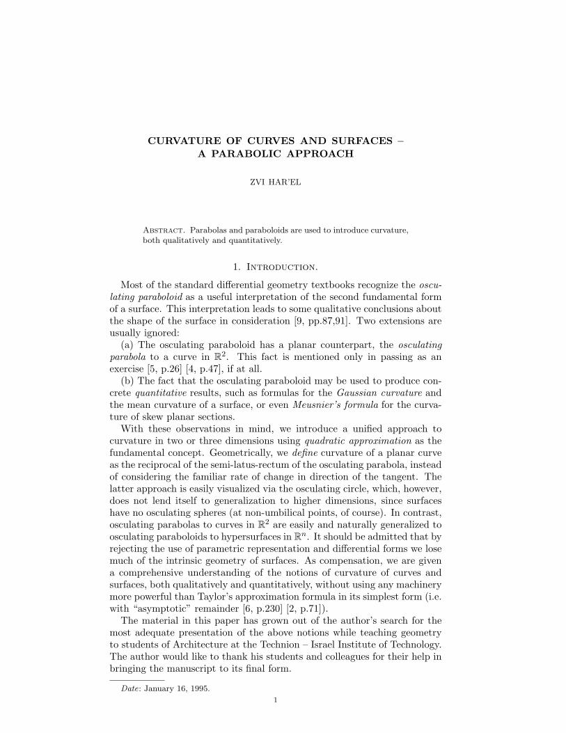
Consider a new coordinate system (ξ, η), whose origin is at the givenpoint P , ξ-axis is the tangent line at P , and η-axis is the upward normal(see Figure 2). Vectorially, the new axes have the positive directions givenby (1, f ′(x0)) and (−f ′(x0), 1), respectively. Let Q(x, f(x)) be another pointon C, then its η-coordinate is its (signed) distance from the tangent line atP , namely,

η =f(x)− f(x0)− f ′(x0)(x− x0)√

1 + f ′(x0)2(3.1)

4 ZVI HAR’EL

x

yP (x0, f(x0))

ξ

η

Q(x, f(x))

C

x− x0

η

ξ

Figure 2. Local coordinate system

(positive for Q above the tangent). This implies, by the quadric approxi-mation of f from Taylor’s formula for Q near P (assuming only that f ′′(x0)exists), that: (assuming only that f ′′(x0) exists):

η =f ′′(x0)

2√

1 + f ′(x0)2(x− x0)2 + o((x− x0)2).(3.2)

On the other hand, we have

x− x0 =1√

1 + f ′(x0)2ξ − f ′(x0)√

1 + f ′(x0)2η,(3.3)

a formula which can be deduced by considering similar triangles or by equat-ing the first components of the vector equation:

(x− x0, y − y0) =(1, f ′(x0))√1 + f ′(x0)2

ξ +(−f ′(x0), 1)√

1 + f ′(x0)2η.(3.4)

Substituting the value of η given by (3.2) into (3.3) we obtain

x− x0 =1√

1 + f ′(x0)2ξ + o(x− x0)

and hence, by the inverse function theorem,

x− x0 =1√

1 + f ′(x0)2ξ + o(ξ).(3.5)

Thus, from (3.2) and (3.5), we obtain

2η =f ′′(x0)

(1 + f ′(x0)2)3/2ξ2 + o(ξ2).(3.6)

We conclude that the osculating parabola is given by 2η = κξ2, whereκ = f ′′(x0)(1 + f ′(x0)2)−3/2 is the curvature of C at P (x0, f(x0)) accordingto Definition 3.1 - agreeing with the standard definition - positive if C lieslocally above the tangent, i.e. if C is concave upward.

CURVATURE - A PARABOLIC APPROACH 5

4. Paraboloids.

In the same way we determined the curvature of a plane curve by com-paring it with its osculating parabola, we wish to compare surfaces in a3-dimensional space with paraboloids (i.e. non-central quadrics [8, p.99]).Consider the family of paraboloids, each having its vertex at the origin andthe z-axis as the normal at the vertex. (Thus, the z-axis is always an axisof symmetry.) This is a 3-parameter family given by the cartesian equation2z = Ax2 + 2Bxy + Cy2. We classify paraboloids according to the typeof their sections with horizontal planes (z = const.). These sections are allsimilar to the (pair of) conic(s) Ax2 + 2Bxy + Cy2 = ±1, called Dupin’sindicatrix [3, p.363] of the paraboloid. Thus, we get elliptic paraboloids ifAC −B2 > 0, hyperbolic paraboloids if AC −B2 < 0, and parabolic cylin-ders (considered as non-central quadrics of parabolic type) if AC −B2 = 0.It is well known (and easily shown) that the discriminant K = AC − B2 isinvariant under rotations of the xy-plane, as is H = (A + C)/2. Conversely,K and H define the indicatrix, and hence the paraboloid, uniquely up toa rotation. Note that K is independent of the orientation of the coordi-nate system (i.e. which way is “up”), while H changes its sign when theorientation is reversed (compare Section 2).

Definition 4.1. The Gaussian curvature, K, and the mean curvature, H,of the paraboloid 2z = Ax2 + 2Bxy + Cy2 at its vertex are K = AC − B2

and H = (A + C)/2, respectively.

We now interpret K and H using the curvature (as defined in Section 2)of normal sections of the paraboloid at its vertex. Recall that a section ofa surface S is the intersection of S and a plane; a normal section of S at apoint P is the section of S by a normal plane, i.e. a plane containing thenormal to S at P. By a suitable rotation of the xy plane, we may assumethat B is zero, so that the x-axis and y-axis are the principal axes of theDupin’s indicatrix. We wish to find the normal sections of the paraboloid2z = Ax2 +Cy2 at the origin, by a plane making an angle θ with the x-axis.

Using cylindrical coordinates, we set x = r cos θ, y = r sin θ, and obtain

2z = (A cos2 θ + C sin2 θ)r2.

Thus the normal section is a parabola, with curvature

κn = A cos2 θ + C sin2 θ =A + C

2+

A− C

2cos 2θ

at its vertex. Assuming, for the sake of definiteness, that A ≥ C, we find

maxκn = κn|θ=0 =A + C

2+

A− C

2= A,

minκn = κn|θ=π/2 =A + C

2− A− C

2= C.

Since AC = K and A + C = 2H, we conclude:

Theorem 4.1 (Euler’s formula for paraboloids). The intersection of a pa-raboloid with a a normal plane at its vertex P is a parabola, whose curvatureat P is given by

κn = κ1 cos2 θ + κ2 sin2 θ,

6 ZVI HAR’EL

where κ1 and κ2 are the roots of the equation κ2 − 2Hκ + K = 0, and θis the angle between the given plane and the plane for which κn attains itsmaximum (if κ1 ≥ κ2, minimum otherwise).

The quantity κn is called the normal curvature of the paraboloid in thedirection of the tangent to the given normal section at the vertex, while itsextreme values, κ1 and κ2, are the principal curvatures. They are attainedin the directions of the principal axes of Dupin’s indicatrix, whence thesedirections are called principal directions.

To complete the discussion, we investigate the nature of the non-normalsections of a paraboloid, i.e. sections with planes through the vertex, makingangles φ (0 < |cos φ| < 1) with the z-axis. Assume, without loss of generality,that the paraboloid 2z = Ax2 + 2Bxy + Cy2 is cut by a plane containingthe x-axis. Using cartesian coordinates (ξ, η) in this plane, we set x = ξ,y = η sinφ, and z = η cosφ, obtaining

2η cos φ = Aξ2 + 2Bξη sinφ + Cη2 sin2 φ.(4.1)

This is a conic whose type is determined by the sign of the discriminant(AC − B2) sin2 φ, i.e. the type of the paraboloid. Furthermore, since thisconic is tangent to the ξ-axis, η = o(ξ) and, from (4.1),

2η cosφ = Aξ2 + o(ξ2),

a curve which has curvature κ = A/ cosφ at ξ = 0. On the other hand,the normal section having the same tangent at the vertex is given by y = 0,2z = Ax2, with normal curvature κn = A. Thus we have:

Theorem 4.2 (Meusnier’s formula for paraboloids). A plane through the ver-tex P of a paraboloid, making an angle φ (such that 0 < |cos φ| < 1) withits normal axis, cuts the paraboloid in a conic (having the same type as theparaboloid) whose curvature at P is given by

κ =κn

cos φ

where κn is the normal curvature of the paraboloid in the direction of thetangent to the conic at P .

Remark . A positive (negative) cosine applies when the positive directionof concavity in the given plane makes an acute (respectively, obtuse) anglewith the upward pointing normal.

5. Curvature of Surfaces.

We now use the results of the last section to investigate general surfaces.

Definition 5.1.i. A paraboloid which has contact of order ≥ 2 at its vertex P with a

surface S is called the osculating paraboloid of S at P .ii. The Gaussian curvature, mean curvature, Dupin’s indicatrix, normal

curvature, etc. of S at P are respectively, the Gaussian curvature, meancurvature, Dupin’s indicatrix, normal curvature etc. at the vertex ofthe osculating paraboloid (assuming its existence).

iii. P is an elliptic, hyperbolic or parabolic point of S if the osculatingparaboloid is elliptic, hyperbolic, or a parabolic cylinder, respectively.

CURVATURE - A PARABOLIC APPROACH 7

The derivation of the equation of the osculating paraboloid of a twicedifferentiable surface, in a manner analogous to that of Section 3, is dif-fered to Section 7, because it is more technical. At this point we noticethat Theorems 4.1 and 4.2 immediately imply the following two classicaltheorems:

Theorem 5.1 (Euler). The intersection of a surface with a normal planeat a point P is a curve, whose curvature at P is given by

κn = κ1 cos2 θ + κ2 sin2 θ,

where κ1 and κ2 are the roots of the equation κ2 − 2Hκ + K = 0, and θis the angle between the given plane and the plane for which κn attains itsmaximum (if κ1 ≥ κ2, minimum otherwise).

Theorem 5.2 (Meusnier). A plane through a point P of a surface S, mak-ing an angle φ (such that cosφ 6= 0) with the normal at P , cuts S in a curvewhose curvature at P is given by

κ =κn

cosφ,

where κn is the normal curvature of S in the direction of the tangent to thegiven section at P .

Both theorems follow from the fact that the second order contact of S withits osculating paraboloid at P implies the same order of contact for the planesections of S with the corresponding sections of the paraboloid. We also notethat the foregoing treatment of surfaces in R3 extends to hypersurfaces inRn.

6. Applications.

As an application of the above theory, we easily compute the Gaussianand mean curvature of a surface of revolution S, obtained (in cylindricalcoordinates) by rotating the curve r = f(z) about the z-axis. Since anyplane through the axis of revolution is a plane of symmetry of S, we deducethat the osculating paraboloid at a given point P (r0, θ0, z0) of S is symmetricabout the plane containing P and the z-axis. This is a normal plane whichcuts S in the meridian θ = θ0, with curvature

κ1 =f ′′(z0)

(1 + f ′(z0)2)3/2(6.1)

(see Section 3). The above symmetry implies this is one of the principalcurvatures, the other one being the normal curvature in the perpendiculardirection, that is tangent to the parallel z = z0 at P . Since the parallel is acircle with curvature 1/r0, and its radius makes an obtuse angle φ with theoutward normal at P (see Figure 3) such that tanφ = − |f ′(z0)|, we obtainthe value

κ2 =cos φ

r0= − 1

f(z0)√

1 + f ′(z0)2(6.2)

for the corresponding normal curvature by using Meusnier’s formula (whichapplies since cosφ 6= 0. Note that |κ2| is the reciprocal of the length of thenormal segment PN in Figure 3). From (6.1) and (6.2) we get

8 ZVI HAR’EL

θ = θ0

r0φP

N

z = z0

Figure 3. Surface of revolution

K = κ1κ2 = − f ′′(z0)f(z0)(1 + f ′(z0)2)2

,

H =κ1 + κ2

2=

f(z0)f ′′(z0)− f ′(z0)2 − 12f(z0)(1 + f ′(z0)2)3/2

,

(6.3)

the usual formulas for the Gaussian curvature and the mean curvature, re-spectively.

Note that as an extra bonus we have shown that the meridians and par-allels of S are principal curves or lines of curvature, that is, curves whosetangents are always in principal directions.

As a specific application of formulas (6.1) to (6.3) consider the catenoidr = a cosh z/a which satisfies the differential equations r/a = (1 + r′2)1/2 =ar′′ and thus has the principal curvatures κ1 = a/r2 along the meridians(catenaries) and κ2 = −a/r2 along the parallels. Consequently K = −a2/r4

and H = 0 everywhere. (Note that κ1 = −κ2 is due to the characterizationof the catenary as the only curve whose curvature at P is equal to thereciprocal of the normal segment PN).

The theory of asymptotic directions and minimal surfaces provides a sec-ond application of the osculating paraboloid. A direction of vanishing nor-mal curvature on a surface is called asymptotic. Euler’s Theorem 4.1 impliesthe existence at a hyperbolic point of two asymptotic directions. This is dueto the fact that the sections of the osculating hyperbolic paraboloid in thedirections of the asymptotes of Dupin’s indicatrix are straight lines (whencethe name “asymptotic”). In particular the asymptotes are mutually per-pendicular if and only if the indicatrix is an equilateral hyperbola. In otherwords, the asymptotic directions are orthogonal if and only if the principalcurvatures are equal in absolute value, i.e. H = (κ1 + κ2)/2 = 0. A surfacewith identically zero mean curvature is said to be minimal, as it can beshown to minimize surface area (locally, with respect to a fixed boundary[5, p.219]). One example is the catenoid (mentioned above), which is theonly minimal surface of revolution (except the plane [4, p.202]).

Another instructive example is provided by the helicoid, the ruled surfacegiven by the cylindrical equation z = aθ. Recall that a ruled surface is a

CURVATURE - A PARABOLIC APPROACH 9

x y

z

ruling

P (r0, 0, 0)normal sectionx = r0, z = aθ

helixr = r0, z = aθ

Figure 4. The helicoid z = aθ

surface swept out by a line moving along a curve (the z-axis, in this case);the various positions of the line are called rulings. To investigate the natureof the surface at a given point P (r0, θ0, z0), we observe that the surface issymmetric about the ruling θ = θ0, z = z0 through P (i.e. symmetric withrespect to a half-turn θ → 2θ0−θ, z → 2z0−z). The osculating paraboloid atP inherits this symmetry, and since the ruling is not the normal in its vertex,the paraboloid is necessarily an equilateral hyperbolic paraboloid (check thatany other paraboloid has only the normal as an axis of symmetry), provingthat the helicoid is minimal! For added clarity, we describe two orthogonalsections of the helicoid with vanishing normal curvature at P , as in Figure 4(where we put θ0 = 0 without any loss of generality). First, any planecontaining the ruling (the x-axis in Figure 4) through P , the normal planeincluded, cuts the surface in a straight line. Second, the plane (x = r0 inFigure 4) perpendicular to the ruling at P yields a normal section of thehelicoid which is symmetric about P , and the symmetry implies that P isan inflection point, in other words the osculating parabola of the section atP is a straight line. But the line is also tangent to the helix z = aθ, r = r0.Thus the helices on the helicoid have the property (shared obviously by therulings) that their tangents always lie in an asymptotic direction. Curveswith this property are called asymptotic curves.

In addition to the principal curves and asymptotic curves, there is a third,even more important kind of a curve. One can easily verify that Meusnier’sformula holds for the curvature of any (not necessarily planar) curve on thesurface, as long as the plane of its osculating parabola makes an angle φwith the normal to the surface. Thus, we have |κ| ≥ |κn|, with equality ifand only if φ = 0, in which case we get the “straightest” curve possible [7,p.221]. This motivates the following:

Definition 6.1. A curve C on a surface S is called a geodesic if, for everypoint P on C, the plane of the osculating parabola to C at P contains the

10 ZVI HAR’EL

normal to S at P (or if the osculating parabola to C at P degenerates to aline, in which case the normal plane containing this line may be chosen).

The great importance of geodesics is the fact that in addition to beingthe straightest they are also the “shortest” curves on the surface, and hencethey are a generalization to lines in the plane [7, p.222]. Geodesics minimizedistance in two senses: Locally, it may be shown [5, p.265] that if two pointson a geodesic are close enough, then the geodesic segment between themis the shortest curve joining these points. Globally, any two points on acomplete surface (intuitively, a surface without holes or edges) may be joinedby a geodesic, which is the shortest curve between the points (Hopf-RinowTheorem [5, p.285]).

Great circles on a sphere, being normal sections, are geodesics. Twoantipodal (diametrically opposite) points on the sphere may be joined byinfinitely many great semicircles, each of which minimizes the distance be-tween the two points. Given two non-antipodal points, one can draw aunique great circle through the points and get two unequal geodesic seg-ments joining them. Of course, only the shorter one minimizes distanceglobally.

As mentioned above, the meridians of a surface of revolutions are normalsections, and hence geodesics. A parallel z = z0 in a surface of revolutionis a geodesic if is a normal section, i.e. if φ = π or f ′(z0) = 0. Hence,parallels of extreme radius, called equators, are geodesics. Such an equatoris for instance the “waist”, z = 0 and r = a of the catenoid. Finally, sincethe osculating parabola to a line lying on a surface is just that line, all therulings of a ruled surface are geodesics.

Geodesics were introduced as the straightest curves on a surface S. Asthe plane of the osculating parabola at a point P contains the normal to Sat P , the orthogonal projection of the geodesic on the tangent plane to S atP has a line for its osculating parabola, hence its curvature vanishes at P .(This is because the osculating parabola of the projection is the projectionof the osculating parabola!) Thus, we define the geodesic curvature κg of acurve C at a point P on S as the curvature at P of the orthogonal projectionof C on the tangent plane to S at P . It measures the deviation of C frombeing a geodesic, and is the intrinsic curvature of C as a subset of S (i.e.the curvature of C as seen by two dimensional inhabitants of S). Let φ beas above, we have

κg = κ sinφ(6.4)

(as the focus a projection of a parabola is the projection of its focus). Com-bining (6.4) with Meusnier’s formula

κn = κ cosφ

we get immediately

κ2 = κ2n + κ2

g.(6.5)

Being straightest curves, geodesics have a useful kinematic interpretation:The orbit on a surface S which is traced by a particle which has no acceler-ation component tangential to S is a geodesic. As the osculating parabola

CURVATURE - A PARABOLIC APPROACH 11

has a contact of order ≥ 2 with the curve, a particle moving along an or-bit C has the same velocity and acceleration vectors at a point P as if itmoved along the osculating parabola to C at P with the same speed ds/dtand tangential acceleration d2s/dt2 at P . In particular, if it moves along Cat a constant speed, one deduces it accelerates only in the direction of thenormal of the osculating parabola (called the principal normal of C) at Pand in the case C is a geodesic this normal coincides with the normal of Sat P , as stated.

Kinematic considerations are most helpful in studying geodesics on a sur-face of revolution S [1, p.153]. Let C be such a geodesic. As the normalto S always meets the z-axis, a constant-speed motion along C will projectorthogonally on a central motion in the xy-plane, i.e. a motion whose accel-eration vector always points to the origin. Such “planetary motion” obeysKepler’s Law of Equal Areas, which may be written, in polar coordinates,

time derivative of swept area =r2

2dθ

dt= constant.

If we return to C, we can replace r dθ/dt, the velocity component tangentialto the parallel, by ds/dt cosψ, where ψ is the angle C forms with the parallelat P . Hence,

r2

2dθ

dt=

r

2ds

dtcos ψ,

and as ds/dt is constant we get Clairaut’s formula [5, p.267]

r cos ψ = c(6.6)

with c constant along C.Formula (6.6) may be used to find the equation of any geodesic on a

surface of revolution S, given as initial data a point r0 and a direction ψ0.We refer the reader to [4, p.257] for further details. We just mention herethat for ψ0 = π/2 we have

c = r0 cosψ0 = 0

from which we obtain the meridian ψ ≡ π/2, and if ψ0 = 0 and the parallelr = r0 is a geodesic, we get that parallel. In any other case, the geodesicsatisfies

r ≥ c = r0 cos ψ0,

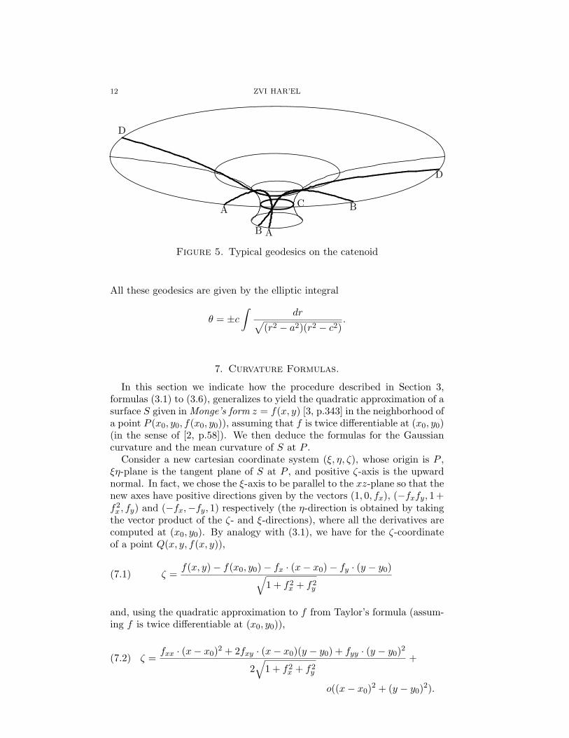
which implies it always stays on one side of the parallel r = c and if theymeet, they touch each other without crossing (as in this case cosψ = c/r = 1we have ψ = 0 and as the parallel r = c is not a geodesic, it cannot be anequator, which implies r < c on one of its sides). In Figure 5 we sketchfour typical geodesics on the catenoid r = a cosh z/a, corresponding to fourvalues of c:

A. For c = 0, a meridian.B. For 0 < c < a, a geodesic which crosses all the parallels.C. For c = a, the equator r = a.D. For c > a, a geodesic which lies on one side of a parallel r = c.

12 ZVI HAR’EL

C

A

A

D

D

B

B

Figure 5. Typical geodesics on the catenoid

All these geodesics are given by the elliptic integral

θ = ±c

∫dr√

(r2 − a2)(r2 − c2).

7. Curvature Formulas.

In this section we indicate how the procedure described in Section 3,formulas (3.1) to (3.6), generalizes to yield the quadratic approximation of asurface S given in Monge’s form z = f(x, y) [3, p.343] in the neighborhood ofa point P (x0, y0, f(x0, y0)), assuming that f is twice differentiable at (x0, y0)(in the sense of [2, p.58]). We then deduce the formulas for the Gaussiancurvature and the mean curvature of S at P .

Consider a new cartesian coordinate system (ξ, η, ζ), whose origin is P ,ξη-plane is the tangent plane of S at P , and positive ζ-axis is the upwardnormal. In fact, we chose the ξ-axis to be parallel to the xz-plane so that thenew axes have positive directions given by the vectors (1, 0, fx), (−fxfy, 1+f2

x , fy) and (−fx,−fy, 1) respectively (the η-direction is obtained by takingthe vector product of the ζ- and ξ-directions), where all the derivatives arecomputed at (x0, y0). By analogy with (3.1), we have for the ζ-coordinateof a point Q(x, y, f(x, y)),

ζ =f(x, y)− f(x0, y0)− fx · (x− x0)− fy · (y − y0)√

1 + f2x + f2

y

(7.1)

and, using the quadratic approximation to f from Taylor’s formula (assum-ing f is twice differentiable at (x0, y0)),

(7.2) ζ =fxx · (x− x0)2 + 2fxy · (x− x0)(y − y0) + fyy · (y − y0)2

2√

1 + f2x + f2

y

+

o((x− x0)2 + (y − y0)2).

CURVATURE - A PARABOLIC APPROACH 13

On the other hand, we have

x− x0 =1√

1 + f2x

ξ − fxfy√(1 + f2

x + f2y )(1 + f2

x)η − fx√

1 + f2x + f2

y

ζ,

y − y0 =1 + f2

x√(1 + f2

x + f2y )(1 + f2

x)η − fy√

1 + f2x + f2

y

ζ,

(7.3)

formulas which can be deduced by equating components of 3-dimensionalanalog to the vector equation (3.4):

(7.4) (x− x0, y − y0, z − z0) =

(1, 0, fx)√1 + f2

x

ξ +(−fxfy, 1 + f2

x , fy)√(1 + f2

x)(1 + f2x + f2

y )η +

(−fx,−fy, 1)√1 + f2

x + f2y

ζ.

But, since ζ is quadratic is x− x0 and y − y0, and therefore quadratic in ξand η by the inverse function theorem, it follows that:

x− x0 =1√

1 + f2x

ξ − fxfy√(1 + f2

x + f2y )(1 + f2

x)η + o(|ξ|+ |η|),

y − y0 =1 + f2

x√(1 + f2

x + f2y )(1 + f2

x)η + o(|ξ|+ |η|).

(7.5)

Thus, from (7.2) and (7.5) we obtain

2ζ = Aξ2 + 2Bξη + Cη2 + o(ξ2 + η2),(7.6)

where

A =1

(1 + f2x + f2

y )1/2(1 + f2x)

fxx,

B =1

1 + f2x + f2

y

(fxy − fxfy

1 + f2x

fxx

),

C =1 + f2

x

(1 + f2x + f2

y )3/2

(fyy − 2

fxfy

1 + f2x

fxy +(

fxfy

1 + f2x

)2

fxx

).

We conclude that the osculating paraboloid is given by 2ζ = Aξ2 + 2Bξη +Cη2, and the invariants

K = AC −B2 =fxxfyy − f2

xy

(1 + f2x + f2

y )2,

H =A + C

2=

(1 + f2x)fyy − 2fxfyfxy + (1 + f2

y )fxx

2(1 + f2x + f2

y )3/2

are respectively the Gaussian curvature and the mean curvature of S at P .

References

1. M. Berger, Lectures on geodesics in riemannian geometry, Tata Institute of Fundamen-tal Research, Bombay, 1965.

2. H. Cartan, Differential calculus, Hermann, Paris, 1971.3. H. S. M. Coxeter, Introduction to geometry, second ed., John Wiley, New York, 1969.

14 ZVI HAR’EL

4. M. DoCarmo, Differential geometry of curves and surfaces, Prentice Hall, 1976.5. H. Guggenheimer, Differential geometry, Dover, New York, 1977.6. G. H. Hardy, A course in pure mathematics, ninth ed., Cambridge, 1944.7. D. Hilbert and S. Cohn-Vossen, Geometry and the imagination, Chelsea Publishing

Co., New York, 1952.8. W. H. McCrea, Analytic geometry of three dimensions, Oliver and Boyd, 1953.9. S. Stoker, Differential geometry, Wiley – Interscience, 1969.

Department of Mathematics, Technion – Israel Institute of Technology,Haifa 32000, Israel

E-mail address: rl@@math.technion.ac.il