PAMPAS: Real-Valued Graphical Models for Computer Vision

Anonymous

Abstract

Probabilistic models have been adopted for many computervision applications, however inference in high-dimensionalspaces remains problematic. As the state-space of a modelgrows, the dependencies between the dimensions lead to anexponential growth in computation when performing infer-ence. Many common computer vision problems naturallymap onto the graphical model framework; the representa-tion is a graph where each node contains a portion of thestate-space and there is an edge between two nodes only ifthey are not conditionally independent. When this graphis sparsely connected, belief propagation algorithms canturn an exponential inference computation into one whichis linear in the size of the graph. However belief propaga-tion is only applicable when the variables in the nodes arediscrete-valued or jointly represented by a single multivari-ate Gaussian distribution, and this rules out many computervision applications.

This paper combines belief propagation with ideas fromparticle filtering; the resulting algorithm performs infer-ence on graphs containing both cycles and continuous-valued latent variables with general conditional probabilitydistributions. Such graphical models have wide applicabil-ity in the computer vision domain and we test the algorithmon example problems of low-level edge linking and locatingjointed structures in clutter.

1. IntroductionProbabilistic techniques for modelling uncertainty havefound widespread success in computer vision. Their ap-plication ranges from pixel-level image generation models[9, 5] to tracking in high-level parametric spaces [7, 18]however as the size of the state-space grows the “curseof dimensionality” can cause an exponential growth in thecomputations necessary to perform inference. Many proba-bilistic vision models naturally decompose into agraphicalmodelstructure [10]; basic components become nodes in agraph where each node is conditionally independent of allbut its near neighbours. When the nodes are image patchesthe neighbours may be spatially close in an image, adjacentlevels in a multi-scale representation or nearby time instantsin an image sequence. Alternatively many complex objectscan be decomposed into graphs where now the nodes aresubparts of the object and an edge is formed in the graph

when two subparts are physically connected. The advan-tage of this graphical model representation is that some for-merly exponential inference computations become linear inthe size of the graph.

Exact inference on graphical models is possible only inrestricted circumstances [10]; the (directed) graph must beacyclic and the joint distribution over those latent variableswhich are not discrete must be a single multivariate Gaus-sian. When a model violates these restrictions, Gibbs sam-pling can be used to draw approximate samples from thejoint distribution [6] but for most computer vision applica-tions this technique remains intractable. Approximate in-ference methods can be used for Conditional Linear Gaus-sian models [12] including time series [2]. Recently twomethods have been widely studied in the computer visionliterature to perform approximate inference on more gen-eral classes of graph; loopy belief propagation [21] (LBP)can be applied to graphs with cycles, though it still only ap-plies to discrete or jointly Gaussian random variables; andparticle filtering [4] allows the use of very general distribu-tions over continuous-valued random variables but appliesonly to graphs with a simple linear chain structure.

The restriction to Gaussian latent variables is particu-larly onerous in computer vision applications because clut-ter in image generation models invariably leads to highlynon-Gaussian, multi-model posterior distributions. This ef-fect largely accounts for the popularity of particle filteringin the computer vision tracking community. In this pa-per we describe thePAMPAS algorithm (PArticle MessagePASsing) which combines LBP with ideas from particle fil-tering. It has wide applicability in the computer vision do-main, for the first time allowing tractable probabilistic in-ference over complex models including high-dimensionaljointed structures and low-level edge chains. We demon-strate the behaviour of the algorithm on test problemsincluding illusory-contour finding and locating a jointedstructure. Additionally we argue that an algorithm whichperforms tractable inference over continuous-valued graph-ical models is a promising tool for research into unifiedcomputer vision models implementing a singe probabilis-tic framework all the way from the pixel level to a semanticdescription. We note recent work in the biological visioncommunity which favours a similar architecture to modelhuman vision.

1

2. Belief propagationBelief propagation (BP) has been used for many years toperform inference in Bayesian networks [10] and has re-cently been applied to graphs with cycles under the name ofloopy belief propagation [21]. The method consists in pass-ing messagesbetween the nodes of the graph where eachmessage can be interpreted as a conditional probability dis-tribution (cpd). When all the latent variables are discrete-valued the cpds can be encoded as matrices, and when thecontinuous-valued variables are jointly Gaussian the distri-butions can be summarised using a mean and covariancematrix.

For models with more complex continuous-valued cpdsthe data representation becomes problematic since as mes-sages are propagated the complexity of the cpds grows ex-ponentially [14]. Techniques exist for pruning the repre-sentations when the cpds and likelihoods are exponentionaldistributions [12, 15] (e.g. Gaussians), and when the graphis a chain, particle filters address the issue by adopting anon-parametric representation, theparticle set[4]. Particlefiltering has been widely used in computer vision since it iswell suited to the complex likelihood functions which resultfrom natural images.

This section begins with a brief description of standardBP and goes on to describe thePAMPAS algorithm whichmodifies BP to use particle sets as messages and thus per-mits approximate inference over general continuous-valuedgraphical models. Sudderth et al [19] have independentlydeveloped an almost identical algorithm and a comparisonis presented in section 2.5.

2.1. Discrete Belief PropagationBelief propagation can in general be stated using a pairwiseMRF formulation [21]. Consider a set of latent-variablenodesX = {X1, . . . , XM} paired with a set of observednodesY = {Y1, . . . , YM}. The conditional independencestructure of the problem is expressed in the neighbourhoodsetP. A pair of indices(i, j) ∈ P if the hidden nodeXj

is not conditionally independent ofXi, and in this case wesayXi is a parent ofXj and by slight abuse of notationi ∈ P(j).

For tutorial simplicity, when theXi are discrete-valuedrandom variables we assume each takes on some valuexi ∈ {1, . . . , L} ≡ L. Given a fixed assignment toYthe observed and hidden nodes are related by observationfunctionsφi(xi, yi) ≡ φi(xi) : L → R. Adjacent hiddennodes are related by the correlation functionsψij(xj , xi) :L × L → R. The joint probability overX is given by

P (X ) =1Z

∏

(i,j)∈Pψij(xj , xi)

(∏

i

φi(xi)

). (1)

The belief propagation algorithm introduces variablessuch asmij(xj) which can intuitively be understood as amessagefrom hidden nodei to hidden nodej about whatstate nodej should be in. Messages are computed itera-tively using the update algorithm

mij(xj) ←∑

xi∈L

φi(xi)ψij(xi, xj)

∏

k∈P(i)\jmki(xi)

(2)and the marginal distribution ofXi (the node’sbelief) isgiven by

bi(xi) = kφi(xi)∏

j∈P(i)

mji(xi). (3)

2.2. Belief propagation in particle networksWhen a problem calls for continuous-valued random vari-ablesXi ∈ RD thenφi(xi) : RD → R andψij(xi,xj) :RD × RD → R and (1) now defines a probability den-sity. In the continuous analogues of (2) and (3) nowmij(·)andbi(·) are functions rather thanL-element arrays; in factwe will assume that they are normalisable probability den-sity functions. When additionally everyψij(xj ,xi) has theform of a cpdψij(xj ,xi) ≡ pij(xj |xi) then (2) becomes

mij(xj) ←∫

RD

pij(xj |xi)φi(xi)∏

k∈P(i)\jmki(xi)dxi.

(4)If the structure of the network is such that the marginal dis-tribution at each node is Gaussian, this integral can be per-formed exactly [15]. As noted above, if any of themij orφi violate this conditional linear Gaussian structure exactinference is intractable and themij must be replaced by anapproximation; thePAMPAS algorithm uses particle sets.

At the heart of any algorithm for belief propagation withparticle sets is a Monte-Carlo approximation to the integralin (4). We set out here a general algorithmic framework forperforming this approximation and in section 2.4 describethe PAMPAS algorithm which is a specific implementationsuitable for common computer vision models.

The function

pMij (xi) ≡ 1

Zijφi(xi)

∏

k∈P(i)\jmki(xi) (5)

is denoted thefoundationof messagemij(·) whereZij is aconstant of proportionality which turnspM

ij (·) into a proba-bility density. A Monte-Carlo integration of (4) yieldsmij ,an approximation ofmij , by drawingN samples from thefoundation

snij ∼ pM

ij (·) (6)

2

and setting

mij(xj) =1N

N∑n=1

pij(xj |xi = snij). (7)

In general it is possible to pick animportance functiongij(xi) from which to generate samples

snij ∼ gij(·) (8)

with (unnormalised) importance weights

πnij ∝ pM

ij (snij)/g(sn

ij) (9)

in which case themij is a weighted mixture

mij(xj) =1∑N

k=1 πkij

N∑n=1

πnijpij(xj |xi = sn

ij). (10)

When the marginal distribution overxi is required, samplessni can be drawn from the estimated belief distribution

bi(xi) =1Zi

φi(xi)∏

j∈P(i)

mji(xi) (11)

either directly or by importance sampling as above andthese samples can be used to compute expectations over thebelief, for example its mean and higher moments. By fix-ing a set of samplessn

i at each node a Gibbs sampler canbe used to generate samples from the joint distribution overthe graph and this is described in section 2.4.

2.3. Choice of importance functionSome limitations of the approach in section 2.2 can be seenby considering a simple example. Suppose that we wish toperform inference on a three-node network(X1,X2,X3)which has the chain structure:

P(1) = (2), P(2) = (1, 3), P(3) = (2).

Two distinct inference chains are being sampled:X1 →X2 → X3 andX3 → X2 → X1 but the information isnot combined in any of the messages; there is no “mix-ing” between the forward and backward directions. Thissituation also arises whenever there is a layered structure tothe graph with a set of low-level nodes passing informationup to higher levels and high-level information propagatingback down. Of course the belief does correctly incorpo-rate information from both directions, but the efficiency of aMonte Carlo algorithm is strongly dependent on the samplepositions so if possible we would like to use all the availableinformation when choosing these positions.

One solution is to use importance sampling for some ofthe particles and a natural choice of function is the current

belief estimateg(xi) = bi(xi) in which case the importanceweights are

πnij = 1/mji(sn

ij). (12)

In the context of the simple chain given above this algo-rithm amounts tosmoothingthe distribution. Smoothinghas been proposed for particle filters [8] but previous algo-rithms merely updated the particle weights in a backwardpass rather than generating new particle positions localisedin regions of high belief.

2.4. ThePAMPAS algorithmA property of many computer vision models is that the cpdspij(xj |xi) can be written as a mixture of Gaussians andthat the likelihoodsφi(xi) are complex and difficult to sam-ple from but can be evaluated up to a multiplicative con-stant. We now describe thePAMPAS algorithm which isspecialised to perform belief propagation for this type ofmodel; section 2.5 includes a brief sketch of a general algo-rithm for which these Gaussian restrictions do not apply.

For notational simplicity we describe the case that eachcpd is a single Gaussian plus a Gaussian outlier processthough the extension to mixtures of Gaussians is straight-forward. Settingλo to be the fixed outlier probability andµij andΛij the parameters of the outlier process,

pij(xj |xi) =(1− λo)N (xj ; fij(xi), Gij(xi))+λoN (xj ; µij , Λij)

(13)

wherefij(·) andGij(·) are deterministic functions, poten-tially non-linear, respectively computing the mean and co-variance matrix of the conditional Gaussian distribution.Each message approximationmij is now a mixture ofN +1Gaussians:

mij(xj) =(1− λo)∑K

k=1 πkij

N∑n=1

πnijN (xj ; fij(sn

ij), Gij(snij))

+ λoN (xj ; µij ,Λij)(14)

and is summarised byN + 1 triplets:

mij = {(πnij , s

nij ,Λ

nij) : 1 ≤ n ≤ N + 1}. (15)

Note thatπN+1ij , sN+1

ij andΛN+1ij correspond to the outlier

process and are fixed throughout the algorithm.As indicated in section 2.3 it makes sense to importance-

sample some fraction of the message partices from the ap-proximate belief distribution. In fact, becauseφi is assumedto be hard to sample from but easy to evaluate, we willuse importance sampling for all the particles but with twodistinct importance distributions and corresponding weight

3

functions. A fraction(1 − ν)N of the particles, by slightabuse of terminology, are denoted direct samples:

snij ∼

1Zij

∏

k∈P(i)\jmki(xi)

πnij = φi(sn

ij)

(16)

and the remainingνN particles we will refer to as impor-tance samples:

snij ∼

1Zij

∏

k∈P(i)

mki(xi)

πnij = φi(sn

ij)/mji(snij).

(17)

Note that if the network is a forward chain whereP(i) ≡i− 1 andν = 0 the algorithm reduces exactly to a standardform of particle filtering [7].

Both (16) and (17) require sampling from a foundationF which is the product ofD mixtures

md =N+1∑n=1

πndN (·; µn

d , Λnd ). (18)

This productF is a Gaussian mixture withO(ND) com-ponenents so direct sampling rapidly becomes infeasible forlargeN or D. Sudderth et al [19] propose a Gibbs samplerwhich performs approximate sampling fromF in O(DN)operations per sample which is described next.

Each componentFL of F is a product ofD Gaussians,one drawn from each of themd and is indexed by a labelvectorL = (l1, . . . , lD), so

F (·) =1Z

∏

L∈IηLN (·; µL, ΛL) (19)

where from the standard Gaussian product formula

Λ−1L =

D∑

d=1

(Λldd )−1 Λ−1

L µL =D∑

d=1

(Λldd )−1µld

d (20)

ηL =∏D

d=1 ηldd N (·; µld

d , Λldd )

N (·; µL, ΛL). (21)

A sample is drawn fromF by first choosing a label vec-tor L using a Gibbs sampler and then generating a randomsample from the GaussianFL. The Gibbs sampler works bysamplingld with all the other labels inL held fixed for eachd in turn. With all of L but ld fixed the marginal product-component weights are given by

ηnd ∝

πndN (·; µn

d ; Λnd )

N (·; µLn , ΛLn)(22)

whereLn = (l1, . . . , ld−1, n, ld+1, . . . , lD); the full Gibbssampler algorithm is given in figure 1. Note that the normal

To generate a sample from the product ofD mixturesmd:

1. InitialiseL. For1 ≤ d ≤ N + 1:

(a) Chooseld uniformly from{1, . . . , N + 1}.2. Iterate:

(a) Choosed uniformly from{1, . . . , D}.(b) For1 ≤ n ≤ N + 1:

i. SetLn = (l1, . . . , ld−1, n, ld+1, . . . , lD).ii. ComputeΛLn andµLn from (20).

iii. Computeηnd from (22).

3. Sample a valuen whereP (ld = n) ∝ ηnd .

4. UpdateL = (l1, . . . , ld−1, n, ld+1, . . . , lD).

Figure 1: Gibbs sampling a product of mixtures.

distributions in (21) and (22) can be evaluated at any conve-nient point, e.g. the origin. GeneratingN samples using theGibbs sampler takesO(DN2) operations so forD < 3 itis preferable to compute the exact product distribution sincea stratified sampler can then be used [3]. As an implemen-tation detail, we find that the Gibbs sampler forsn

ij can benoisy unless run for many iterations, in the sense that it reg-ularly generates particles which have very low probability.This can lead to problems when importance sampling sincemji(sn

ij) in (17) may be very small leading to a high weightπn

ij which suppresses the other samples in the set. This maysuggest an adaptive sampling algorithm which continues toiterate the Gibbs sampler until the variance of theπn

ij fallsbelow some threshold value. In practice, in experiments be-low we simply smooth theπn

ij by replacing anyπnij > 0.25ν

byπn

ij ← (ν − πnij)/6 (23)

and renormalising. The fullPAMPAS message update algo-rithm is given in figure 2.

When N belief samplessni have been drawn for each

node inX they can be used to sample from the joint distri-bution over the graph. This also relies on a Gibbs samplerbut now the label vectorL = (l1, . . . , lM ) indexes a sampleslmm at each of theM nodes and the marginal probability of

choosing labelld when the other labels are fixed is

P (ld = n) = φd(sni )

∏

j∈P(i)

pji(sni |xj = slj

j ). (24)

2.5. Comparison with the NBP algorithmSudderth et al [19] have independently developed an almostidentical algorithm for performing belief propagation with

4

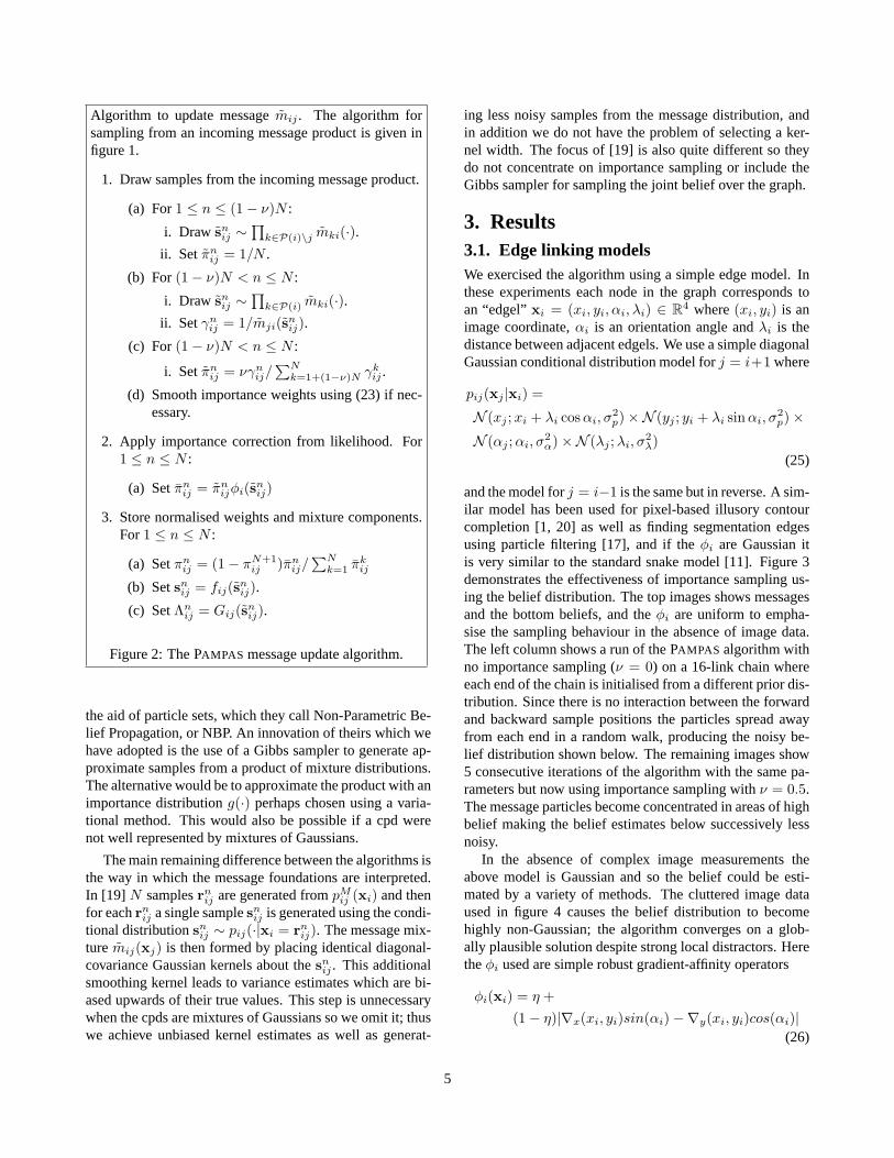
Algorithm to update messagemij . The algorithm forsampling from an incoming message product is given infigure 1.

1. Draw samples from the incoming message product.

(a) For1 ≤ n ≤ (1− ν)N :

i. Draw snij ∼

∏k∈P(i)\j mki(·).

ii. Set πnij = 1/N .

(b) For(1− ν)N < n ≤ N :

i. Draw snij ∼

∏k∈P(i) mki(·).

ii. Setγnij = 1/mji(sn

ij).

(c) For(1− ν)N < n ≤ N :

i. Setπnij = νγn

ij/∑N

k=1+(1−ν)N γkij .

(d) Smooth importance weights using (23) if nec-essary.

2. Apply importance correction from likelihood. For1 ≤ n ≤ N :

(a) Setπnij = πn

ijφi(snij)

3. Store normalised weights and mixture components.For1 ≤ n ≤ N :

(a) Setπnij = (1− πN+1

ij )πnij/

∑Nk=1 πk

ij

(b) Setsnij = fij(sn

ij).

(c) SetΛnij = Gij(sn

ij).

Figure 2: ThePAMPAS message update algorithm.

the aid of particle sets, which they call Non-Parametric Be-lief Propagation, or NBP. An innovation of theirs which wehave adopted is the use of a Gibbs sampler to generate ap-proximate samples from a product of mixture distributions.The alternative would be to approximate the product with animportance distributiong(·) perhaps chosen using a varia-tional method. This would also be possible if a cpd werenot well represented by mixtures of Gaussians.

The main remaining difference between the algorithms isthe way in which the message foundations are interpreted.In [19] N samplesrn

ij are generated frompMij (xi) and then

for eachrnij a single samplesn

ij is generated using the condi-tional distributionsn

ij ∼ pij(·|xi = rnij). The message mix-

turemij(xj) is then formed by placing identical diagonal-covariance Gaussian kernels about thesn

ij . This additionalsmoothing kernel leads to variance estimates which are bi-ased upwards of their true values. This step is unnecessarywhen the cpds are mixtures of Gaussians so we omit it; thuswe achieve unbiased kernel estimates as well as generat-

ing less noisy samples from the message distribution, andin addition we do not have the problem of selecting a ker-nel width. The focus of [19] is also quite different so theydo not concentrate on importance sampling or include theGibbs sampler for sampling the joint belief over the graph.

3. Results3.1. Edge linking modelsWe exercised the algorithm using a simple edge model. Inthese experiments each node in the graph corresponds toan “edgel”xi = (xi, yi, αi, λi) ∈ R4 where(xi, yi) is animage coordinate,αi is an orientation angle andλi is thedistance between adjacent edgels. We use a simple diagonalGaussian conditional distribution model forj = i+1 where

pij(xj |xi) =

N (xj ;xi + λi cos αi, σ2p)×N (yj ; yi + λi sin αi, σ

2p)×

N (αj ;αi, σ2α)×N (λj ; λi, σ

2λ)

(25)

and the model forj = i−1 is the same but in reverse. A sim-ilar model has been used for pixel-based illusory contourcompletion [1, 20] as well as finding segmentation edgesusing particle filtering [17], and if theφi are Gaussian itis very similar to the standard snake model [11]. Figure 3demonstrates the effectiveness of importance sampling us-ing the belief distribution. The top images shows messagesand the bottom beliefs, and theφi are uniform to empha-sise the sampling behaviour in the absence of image data.The left column shows a run of thePAMPAS algorithm withno importance sampling (ν = 0) on a 16-link chain whereeach end of the chain is initialised from a different prior dis-tribution. Since there is no interaction between the forwardand backward sample positions the particles spread awayfrom each end in a random walk, producing the noisy be-lief distribution shown below. The remaining images show5 consecutive iterations of the algorithm with the same pa-rameters but now using importance sampling withν = 0.5.The message particles become concentrated in areas of highbelief making the belief estimates below successively lessnoisy.

In the absence of complex image measurements theabove model is Gaussian and so the belief could be esti-mated by a variety of methods. The cluttered image dataused in figure 4 causes the belief distribution to becomehighly non-Gaussian; the algorithm converges on a glob-ally plausible solution despite strong local distractors. Heretheφi used are simple robust gradient-affinity operators

φi(xi) = η +(1− η)|∇x(xi, yi)sin(αi)−∇y(xi, yi)cos(αi)|

(26)

5

Figure 3:Importance sampling mixes information from forward and backward chains.The top images show messages passedforwards and backwards along a simple chain, in red and green respectively. The bottom images show the resulting beliefs.The left hand column shows the output when no importance sampling is used and the forward and backward messages do notinteract. When importance sampling is used withν = 0.5 the message particles are guided to areas of high belief; the righthand columns show 5 successive iterations of the algorithm.

where∇x(·) and∇y(·) are respectively horizontal and ver-tical image gradient functions (Sobel operators) andη =0.1 is the probability that no edge is visible. The incorpora-tion of information along the chain in both directions can beexpected to improve the performance of e.g. the Jetstreamalgorithm [17] which is a particle-based edge finder.

3.2. Illusory contour matchingWe tested the algorithm on a illusory-contour finding appli-cation shown in figure 5. The input image hasC “pacman”-like corner points where the open mouth defines two edgedirections leading away from the corner separated by an an-gle Cα. The task is to match up the edges with smoothcontours. We construct2C chains each of four links, andeach is anchored at one end with a prior starting at its des-ignated corner pointing in one of the two edge directions.At the untethered end of a chain from cornerC is a “con-nector” edgel which is attached to (conditionally dependenton) the connectors at the ends of the2C−2 other chains notstarting from cornerC. We use the same edgel model as insection 3.1 but now each node state-vectorxi is augmentedwith a discrete labelυi denoting which of the2C−2 partnerchains it matches, and the cpds at the are modified so thatpij(xj |xi) = 0 whenυi andυj do not match.

Figure 5 shows the model being applied to two scenarioswith C = 6 in both cases. First,Cα = 11π/36 whichleads to two overlapping triangles with slightly concaveedges when the chains are linked by the algorithm. Sec-ondly,Cα = 7π/9 which leads to a slightly convex regularhexagon. The same parameters are used for the models inboth cases, so the algorithm is forced to adapt the edgellengths to cope with the differing distances between target

Figure 4:An edge linking model finds global solutions.Theimages show (in raster order) the belief estimates after 1, 5,and 10 iterations, and 7 samples from the joint distributionafter 10 iterations. The ends of the chain are sampled fromprior distributions centred on the middle-left and middle-right of the image respectively. The distractors in the tophalf of the image have stronger edges and are closer to thefixed prior than the continuous edge below. After a fewiterations the belief has stabilised on a bimodal distribution.As is clear from the samples drawn from the joint graph,most of the weight of the distribution is on the continuousedge.

6

corners.

Figure 5:ThePAMPAS algorithm performs illusory contourcompletion. A model consisting of twelve 4-link chainstries to link pairs of chains to form smooth contours. De-pending on the angle at which the chains leave the cornerpositions, the belief converges on either two overlappingtriangles (left) or a single hexagon (right). Links includea discrete label determining which partner chain they areattached to; the displayed link colour is the colour of thepartner chain’s corner. See text for more details.

3.3. Finding a jointed object in clutter

Finally we constructed a graph representing a jointed ob-ject and applied thePAMPAS algorithm to locating the ob-ject in a cluttered scene. The model consists of 9 nodes;a central circle with four jointed arms each made up oftwo rectangular links. The circle nodex1 = (x0, y0, r0)encodes a position and radius. Each arm nodexi =(xi, yi, αi, wi, hi), 2 ≤ i ≤ 9 encodes a position, angle,width and height and prefers one of the four compass di-rections (to break symmetry). The arms pivot around theirinner joints, so for the inner arms2 ≤ i ≤ 5, p1i(xi|x1)encodes the process

xi = x1 +N (·; 0, σ2p) yi = y1 +N (·; 0, σ2

p)

αi = (i− 2)π/2 +N (·; 0, σ2β)

wi = r1δw +N (·; 0, σ2s) hi = r1δh +N (·; 0, σ2

s).

The cpd to go from an inner arm2 ≤ i ≤ 5 to the outerarmsj = i + 4 is given by

xj = xi + hi cos(αi) +N (·; 0, σ2p)

yj = yi + hi sin(αi) +N (·; 0, σ2p)

αj = αi +N (·; 0, σ2α)

wj = wi +N (·; 0, σ2s) hj = hi +N (·; 0, σ2

s).

In the other direction the arm process is not Gaussian butwe approximate it with the following:

xi = xj − hj cos(αi) +N (·; 0, hjσs| sin((i− 2)π/2)|σ2p)

yi = yj − hj sin(αi) +N (·; 0, hjσs| cos((i− 2)π/2)|σ2p)

αi = αj +N (·; 0, σ2α)

wi = wj +N (·; 0, σ2s) hi = hj +N (·; 0, σ2

s).

Thepi1(x1|xi) are straightforward:

x1 = xi +N (·; 0, σ2p) y1 = yi +N (·; 0, σ2

p)

r1 = 0.5(wi/δw + hi/δh) +N (·; 0, σ2s).

The object has been placed in image clutter in figure 6.The clutter is made up of 12 circles and 100 rectanglesplaced randomly in the image. The messages are initialisedwith a simulated specialised feature detector:x1 is sam-pled from positions near the circles in the image and thearms are sampled to be near the rectangles, with rectanglescloser to the preferred direction of each arm sampled morefrequently. Each node containsN = 75 particles so thespace is undersampled. After initialisation thePAMPAS al-gorithm is iterated using a single Gaussian outlier coveringthe whole image (i.e. the “feature detector” information isnot used after initialisation). After two or three iterations thebelief distribution has converged on the object. In this caseit might be argued that it would be more straightforward tosimply detect the circles and perform an exhaustive searchnear each. Figure 7 demonstrates the power of the proba-

Figure 6:A jointed object is located in clutter. The left handimage shows a sample from the belief distribution overlaidon a cluttered scene. The right hand image shows the fullbelief distribution after 10 iterations. See text for more de-tails.

bilistic modelling approach, however, since now the circleat the centre of the object has not been displayed, simulat-ing occlusion. Of course nox1 samples are generated nearthe “occluded” circle, but even after one iteration the beliefat that node has high weight at the correct location due tothe agreement of the nearby arm nodes. After a few itera-tions the belief has converged on the correct object positiondespite the lack of the central circle.

7

Figure 7: An occluded object is located in clutter.Theleft hand image shows a sample from the belief distribu-tion overlaid on a cluttered scene. Note that there is nocircle present in the image where the belief has placed it.This models an occluded object which has still been cor-rectly located. The right hand image shows the full beliefdistribution after 10 iterations. See text for more details.

4. Conclusion

We have concentrated in this paper on examples with syn-thetic data in order to highlight the working of thePAMPAS

algorithm. The applications we have chosen are highly sug-gestive of real-world problems, however, and we hope thepromising results will stimulate further research into ap-plying continuous-valued graphical models to a variety ofcomputer vision problems. Sections 3.1 and 3.2 suggest avariety of edge completion applications. Section 3.3 indi-cates that thePAMPAS algorithm may be effective in lo-cating articulated structures in images, in particular peo-ple. Person-finding algorithms exist already for locatingand grouping subparts [16] but they do not naturally fit intoa probalistic framework. One obvious advantage of usinga graphical model representation is that it extends straight-forwardly to tracking, simply by increasing the size of thegraph and linking nodes in adjacent timesteps. Anotherarea of great interest is linking the continuous-valued graphnodes to lower-level nodes which may be discrete-valued asin [9]. In fact, researchers in the biological vision domainhave recently proposed a hierarchical probabilistic structureto model human vision which maps very closely onto ouralgorithmic framework [13].

References[1] J. August and S.W. Zucker. The curve indicator random field: curve

organization via edge correlation. InPerceptual Organization forArtificial Vision Systems. Kluwer Academic, 2000.

[2] X. Boyen and D. Koller. Tractable inference for complex stochasticprocesses. InProceedings of the 14th Annual Conference on Uncer-tainty in Artificial Intelligence, 1998.

[3] J. Carpenter, P. Clifford, and P. Fearnhead. An improved par-ticle filter for non-linear problems. Technical report, Dept.

of Statistics, University of Oxford, 1997. Available fromwww.stats.ox.ac.uk/ ˜ clifford/index.html .

[4] A. Doucet, N. de Freitas, and N. Gordon, editors.Sequential MonteCarlo Methods in Practice. Springer-Verlag, 2001.

[5] W.T. Freeman, T.R. Jones, and E.C. Pasztor. Example-based super-resolution.IEEE Computer Graphics and Applications, March/April2002.

[6] S. Geman and D. Geman. Stochastic relaxation, Gibbs distributions,and the Bayesian restoration of images.IEEE Trans. on Pattern Anal-ysis and Machine Intelligence, 6(6):721–741, 1984.

[7] M. Isard and A. Blake. Condensation — conditional density propa-gation for visual tracking.Int. J. Computer Vision, 28(1):5–28, 1998.

[8] M.A. Isard and A. Blake. A smoothing filter for Condensation. InProc. 5th European Conf. Computer Vision, volume 1, pages 767–781, 1998.

[9] N. Jojic, N. Petrovic, B. J. Frey, and T. S. Huang. Transformed hid-den markov models: Estimating mixture models of images and infer-ring spatial transformations in video sequences. Incvpr, 2000.

[10] M.I. Jordan, T.J. Sejnowski, and T. Poggio, editors.Graphical Mod-els : Foundations of Neural Computation. MIT Press, 2001.

[11] M. Kass, A. Witkin, and D. Terzopoulos. Snakes: Active contourmodels. InProc. 1st Int. Conf. on Computer Vision, pages 259–268,1987.

[12] D. Koller, U. Lerner, and D. Angelov. A general algorithm for ap-proximate inference and its application to hybrid bayes nets. InPro-ceedings of the 15th Annual Conference on Uncertainty in ArtificialIntelligence, pages 324–333, 1999.

[13] T.S. Lee and D. Mumford. Hierarchical bayesian inference in thevisual cortex. Journal of the Optical Society of America A, 2002(submitted).

[14] U. Lerner.Hybrid Bayesian Networks for Reasoning about ComplexSystems. PhD thesis, Stanford University, October 2002.

[15] T.P. Minka. A family of algorithms for approximate Bayesian infer-ence. PhD thesis, MIT, January 2001.

[16] G. Mori and J. Malik. Estimating human body configurations usingshape context matching. Ineccv7, pages 666–680, 2002.

[17] P. Perez, A. Blake, and M. Gangnet. Jetstream: Probabilistic contourextraction with particles. Iniccv8, volume II, pages 524–531, 2001.

[18] H. Sidenbladh, M.J. Black, and L. Sigal. Implicit probabilistic mod-els of human motion for synthesis and tracking. Ineccv7, volume 1,pages 784–800, 2002.

[19] E.B. Sudderth, A.T. Ihler, W.T. Freeman, and A.S. Willsky. Nonpara-metric belief propagation. Technical Report P-2551, MIT Laboratoryfor Information and Decision Systems, 2002.

[20] L.R. Williams and D.W. Jacobs. Stochastic completion fields: Aneural model of illusory contour shape and salience.Neural Compu-tation, 9(4):837–858, 1997.

[21] J.S. Yedidia, W.T. Freeman, and Y. Weiss. Understanding beliefpropagation and its generalizations. Technical Report TR2001-22,MERL, 2001.

8