PACKETS, ROUTERS, AND AUTOMOBILES: WHAT CAN DATANETWORKS TEACH US ABOUT TRAFFIC CONGESTION?

A Thesisin TCC 402

Presented to

The Faculty of theSchool of Engineering and Applied Science

University of Virginia

In Partial Fulfillment

of the Requirements for the Degree

Bachelor of Science in Computer Science

by

John Calandrino

March 26, 2002

On my honor as a University student, on this assignment I have neither given norreceived unauthorized aid as defined by the Honor Guidelines for Papers in TCCCourses.

Approved Professor David Evans - Technical Advisor

Approved Professor Patricia Click - TCC Advisor

i

TABLE OF CONTENTS

ABSTRACT............................................................................................................................v

1. INTRODUCTION ................................................................................................................11.1 Purpose Statement..............................................................................................11.2 Problem Definition and Background..................................................................11.3 Scope and Method..............................................................................................31.4 Overview of Report............................................................................................4

2. DATA NETWORKS AND TRAFFIC SYSTEMS OVERVIEW AND COMPARISON ..................52.1 Overview of Data Networks...............................................................................52.2 Network Congestion Control and Avoidance Techniques.................................6

2.2.1 Network Entry-Point Techniques ........................................................72.2.2 Router Techniques.............................................................................102.2.3 Alternative Techniques......................................................................11

2.3 Traffic Flow Control Research.........................................................................122.3.1 Herman and Gardels: Platooning in the Holland Tunnel ................122.3.2 Bumper to Bumper Report: On-Ramp Entrance Control .................132.3.3 Manual on Uniform Traffic Control Devices: Ramp Signals ...........142.3.4 Sample Study on Real Time Ramp Metering.....................................142.3.5 Common Ramp Metering Techniques ...............................................15

2.4 Comparison of Data Networks and Freeway Systems.....................................17

3. SIMULATING THE TRAFFIC SYSTEM.............................................................................203.1 CORSIM ..........................................................................................................203.2 Freeway Model.................................................................................................203.3 Simulating Interstate 66 ...................................................................................22

4. EXPERIMENTATION .......................................................................................................264.1 Applying Each Technique ................................................................................264.2 Experimental Results........................................................................................28

5. PRAGMATIC TECHNIQUE APPLICATION .......................................................................325.1 Combining and Fine-tuning Successful Techniques........................................325.2 Evaluation of Most Successful Combination...................................................35

6. CONCLUSIONS ................................................................................................................366.1 Summary of Findings.......................................................................................366.2 Discussion and Interpretation of Results..........................................................376.3 Recommendations for Future Research...........................................................396.4 Report Summary..............................................................................................40

WORKS CITED ...................................................................................................................42

BIBLIOGRAPHY ..................................................................................................................44

ii

APPENDICES .......................................................................................................................46Appendix A: Simulation Verification Data............................................................46Appendix B: Detailed Technique Application Procedures ....................................47Appendix C: Experimental Data Summary............................................................48Appendix D: Experimental On-Ramp Data ...........................................................49

iii

LIST OF FIGURES

Figure 2.1 - A Simple Interconnected Network ...................................................................5Figure 3.1 - Simulated Segment of Interstate 66................................................................21Figure 3.2 - Comparison of Simulated and Actual Vehicle Volumes................................23Figure 4.1 - Freeway Travel Times for Each Technique ...................................................30Figure 4.2 - Throughput for Each Technique.....................................................................30Figure 4.3 - Average On-Ramp Wait Times for Each Technique .....................................30Figure 5.1 - Freeway Travel Times for Combinations of Techniques...............................34Figure 5.2 - Throughput for Combinations of Techniques ................................................34Figure 5.3 - Average On-Ramp Wait Times for Combinations of Techniques .................34

iv

LIST OF TABLES

Table 4.1 - Procedures for Applying Congestion Control Techniques..............................27Table A.1 - Simulation Verification Data ..........................................................................46Table B.1 - Detailed Technique Application Procedures...................................................47Table C.1 - Experimental Data Summary..........................................................................48Table D.1 - Simulated Vehicle Volumes ...........................................................................49Table D.2 - Simulated Approximate Queued Vehicle Counts...........................................49Table D.3 - Simulated Approximate Queue Lengths .........................................................49Table D.4 - Simulated Approximate On-Ramp Speed.......................................................49Table D.5 - Simulated Time to Wait in On-Ramp Queue at 7:00 P.M..............................50

v

ABSTRACT

This project applied data network congestion control and avoidance techniques to

freeway systems through simulation and measured their effectiveness. Experimentation

revealed that Fair Queueing at the most congested on-ramps combined with the addition

of a lane to the freeway provided the most significant improvements to the freeway

system. This finding is significant because it demonstrates potential for the cross-

application of data network congestion control techniques to congested freeways.

Data networks and freeway systems are similar in several ways. Both systems

allow for the flow of information or vehicles along limited pathways and have distinct

entry points that are capable of flow rate metering. There are differences between the

systems, however, that make cross-application somewhat difficult. Traffic networks are

generally centralized systems where current congestion data is readily available, while

large-scale data networks are decentralized, making monitoring considerably harder, and

requiring additional guesswork. Additionally, data networks usually prevent data entry

into the system when congestion gets particularly bad, whereas such a flow shutdown at a

freeway on-ramp would be unacceptable. Despite these differences, in the simulations

conducted for this project data network congestion control techniques often increased

throughput and capacity and reduced travel time on freeway systems, though at the cost

of increased wait times at freeway on-ramps. Solutions to this wait problem include

alternate routes, parallel freeways, and toll roads pro-rated for current wait time.

It is my hope that the research described in this report will promote collaboration

between two similar areas of research - data network and freeway system congestion

resolution. Such sharing would greatly benefit both research areas.

1

1. INTRODUCTION

1.1 Purpose Statement

This project evaluated the effects of applying data network congestion control and

avoidance techniques to limited access highway systems through simulation. It measured

the ability of each technique to decrease travel time and increase throughput and capacity

in traffic systems while avoiding unacceptably long wait times at freeway on-ramps. The

results showed that Fair Queueing at the most congested on-ramps combined with the

addition of a lane to the freeway provided the most balanced improvement to the freeway

system, and demonstrated potential for the cross-application of data network congestion

control techniques to congested freeways.

1.2 Problem Definition and Background

In upstate New York, nearly 90 percent of personal travel is by motor vehicle.

This is because, as in many regions of America, people prefer to travel in private vehicles

as opposed to public forms of transportation. Even in downstate New York, where an

extensive public transportation system exists in both New York City and Long Island, the

percentage is still 57 percent, greater than half of all personal travel. A politician could

win a local election on the platform of reducing traffic congestion. Across the nation,

according to survey results published by Kenneth Orski and cited by Levy and Bragman,

"traffic congestion has superseded crime, housing, and unemployment as the primary

concern of voters" [1].

For many years, engineers have been developing analytical models and simulation

tools to study and improve vehicular flow on highways. Such methods give us a better

2

understanding of vehicular and traffic system behavior. Forty years ago, Herman and

Gardels [2] developed a mathematical model of traffic. They used it to invent a

technique they called platooning, which increased traffic flow in the Holland Tunnel that

connects New York and New Jersey. Today, there is an entire branch of engineering

devoted to predicting and improving traffic flow on roadways.

More recently, computer engineers and computer scientists have been developing

ways to improve data network traffic flow and efficiency, primarily with sophisticated

congestion control and avoidance techniques. In particular, they have focused on

improving the Transmission Control Protocol (TCP) [3], which the Defense Advanced

Research Projects Agency developed in 1981, and which is now the dominant reliable

protocol used in the transmission layer of the Internet [4]. Such networks have much in

common with a freeway system, and with a basic traffic model. A data network allows

for flow of information along limited pathways, and entry of data packets at discrete

points within the system. Similarly, limited access highways limit the flow of traffic to

their road surface, and restrict entry to specified on-ramps. One difference between the

two systems, however, is that freeway systems are generally more centralized, with

ownership and control of the system falling under a single authority, such as a state

Department of Transportation. This allows a congestion control technique to take

measurements that will conclude definitively if congestion exists on the freeway. Large-

scale, decentralized data networks do not have this luxury, and determination of

congestion requires estimation and guesswork. Another difference is that data networks

typically shut down flow at entry points in the system when congestion gets particularly

bad, whereas such metering behavior at a freeway on-ramp would be unacceptable.

3

This report discusses the outcomes of applying data network congestion control

and avoidance techniques to a simulated vehicular traffic system. Despite the differences

between vehicular traffic and data networks, data network congestion control techniques

had a considerable impact on freeway systems in the simulations conducted for this

project. The techniques often increased throughput and capacity and minimized travel

time, though at the cost of increased wait times at freeway on-ramps. The technique that

best applied to the system, and was most practically adaptable to the real world in the

right situations, was Fair Queueing at highly congested on-ramps combined with the

addition of a lane to the freeway. This project also demonstrated that physical vehicles

on a roadway often respond to the same congestion control and avoidance techniques as

abstract data packets on a communications line.

1.3 Scope and Method

I tested the effects of approximately ten congestion control and avoidance

techniques, and some of their combinations, in a simulated traffic system environment.

Most of these techniques are applied by means of on-ramp meters in the simulation. The

tests measured how the applied techniques altered the flow, capacity, and travel time on

the freeway.

I considered three general categories of techniques based on their strategy for

controlling congestion. The first category contains techniques that restrict the flow of

new data packets into the network in an attempt to prevent network overload. This

category of techniques was applied to the simulation through on-ramp metering. The

second category contains techniques that drop packets already present in the network,

4

usually when the packet traffic in the network exceeds a certain threshold. On-ramp

metering was also used to apply these techniques, substituting a metering restriction for a

vehicle "drop" (which is impossible). Therefore, these techniques when cross-applied

actually became much like the first category, controlling congestion at the entry points of

the system instead of internally. Finally, I placed techniques that used alternate methods

for increasing the flow and efficiency of the network in the last category. These

techniques required a different approach when applied to the simulated freeway.

1.4 Overview of Report

The remainder of this report will provide some technical background, and then

proceed to describe the experiment and its results. Chapter 2 provides an overview of

data network congestion control techniques and traffic flow control research, along with a

comparison of data networks and freeway systems. Chapters 3 through 5 then describe

the project work itself. Chapter 3 discusses the creation of the real-world freeway

simulation on which the experiment is performed. Chapter 4 outlines the procedures for

applying each technique separately to the freeway simulation, and discusses the results,

including an explanation of what constitutes a successful technique. Chapter 5 presents

the results of testing combinations and improvements of the congestion resolution

techniques, and an evaluation of most successful combination, Fair Queueing at three on-

ramps combined with the addition of a lane to the freeway. Finally, chapter 6 concludes

with a summarization of the experiment, interpretation of the results, and

recommendations for future research in this area.

5

2. DATA NETWORKS AND TRAFFIC SYSTEMS OVERVIEW AND COMPARISON

2.1 Overview of Data Networks

Before discussing the ways in which data networks control and avoid congestion,

some background on data networks is needed. One can view a data network as a

collection of links and nodes. Nodes send data across the links, which provide

connectivity and allow nodes to share data with one another. Additionally, a set of

cooperating nodes can achieve indirect connectivity amongst themselves. Nodes

accomplish this by allowing data en route to a destination to be forwarded through them.

In other words, nodes agree to serve as intermediate nodes in the data path from the

source to the destination. Such cooperating groups of nodes can be interconnected with

other groups to form a scalable internetwork. The interconnecting component is usually a

router or gateway, a simple node that forwards data from one cooperating group of nodes

to another. The Internet gets its name from the fact that it has this internetwork structure.

The nodes in the network are usually computers, routers, or gateways, while the links in

the network generally refer to some physical medium that connects two or more nodes

[4]. As an example of a network, consider Figure 2.1.

Figure 2.1 - A Simple Interconnected Network

In a network without indirect connectivity, nodes would only be able to

communicate with their neighbors. Node D would only be able to share data with node

6

E, and node A would only be able to share data with nodes B and C. If nodes D, E, and F

cooperate, however, D can establish indirect connectivity with node F. Additionally, if

nodes A, B, and C choose to cooperate, both cooperating groups of nodes can be

interconnected through an external router to form the simple internetwork shown in

Figure 2.1.

To guide the design and implementation of a network, a data network system

designer typically refers to a layered network architecture. This allows for progressively

higher and more abstract levels of service in each layer. The most popular theoretical

model, known as the Open Systems Interconnection (OSI) architecture, defines seven

layers of abstraction, from the physical connection layer to the application layer. The

most important layers for the purposes of this report are the second and fourth layers.

The second layer is the data link layer, which handles the transmission of streams of data

bits. The Ethernet protocol, a widely used local area networking technology, operates in

this layer. The fourth layer is the transport layer, which handles transmission of data

messages (generally a number of data packets, or blocks of data) between nodes. The

Transmission Control Protocol (TCP) [3] operates in this layer. This is one level of

abstraction above the network layer, which handles the successful delivery of individual

data packets. This is the layer in which the most widely used network layer protocol

today, the Internet Protocol (IP), operates [4].

2.2 Network Congestion Control and Avoidance Techniques

There are a number of congestion control and avoidance techniques available to

reduce congestion, increase packet flow, and reduce round-trip times in data networks.

7

Many of these techniques are designed to work with the Transmission Control Protocol

(TCP) [3], the dominant reliable protocol used in the transmission layer of the Internet

[4]. TCP controls network congestion by altering the rate at which an end point sends

packets into the network. TCP does this by limiting entry of data into the network with a

congestion window. A congestion window permits the source to send a number of

packets, or segmented blocks of data, equal to the current size of the congestion window.

TCP controls how much data can enter the network at a given time through manipulating

the size of this window. Most of the congestion control and avoidance techniques for

TCP set the size of the window based on feedback from the network. This feedback is

usually in the form of acknowledgements that are sent from the receiver to the sender to

indicate successful packet delivery. Oftentimes, the techniques assume that "lost"

packets (packets for which the source does not receive an acknowledgment) indicate

congestion and act accordingly to reduce it [4].

2.2.1 Network Entry-Point Techniques

The first category of techniques are those that restrict the flow of packets into a

data network, usually with a congestion window. All of these techniques handle

congestion at the endpoints of a network, that is, where new data is waiting to enter.

Most data networks provide their lowest level of congestion control at the data

link layer, where the Ethernet protocol often operates. This protocol implements two

simple forms of congestion control in its transmitter algorithm. When the line is idle, the

protocol transmits a frame (similar to a packet) immediately. When the line is busy,

however, the algorithm waits until the line is idle and then transmits with a probability p.

8

This is known as p-persistence, and Ethernet networks use it to prevent multiple adapters

from trying to transmit at the same time when the line becomes free, to prevent collisions.

If two adapters transmit at the same time anyway, their data collides and this stops

transmission. These adapters then wait a certain amount of time and try again. Each time

the transmission fails, an adapter increases its wait time (usually doubling it) before

trying again. This is known as exponential backoff, and it is the other form of congestion

control in an Ethernet [4].

In 1988, Jacobson and Karels [7] suggested several modifications to the then-

current implementations of the TCP protocol. Their primary philosophy was that packet

flow on a TCP connection should be conservative in order to avoid congestion collapse.

An overflow of packets into the network causes this collapse, which results in a sudden

drop in data throughput through the network. This drop is often crippling to the network,

as demonstrated by the "factor-of-thousand drop" cited in the paper [7]. Today, TCP

implements most of the modifications proposed in the paper, including Additive

Increase/Multiplicative Decrease (AIMD) and a slow-start algorithm that gradually

increases the number of packets sent. The paper also included a discussion of estimating

packet round-trip times in data networks. This laid the groundwork for a congestion

avoidance scheme known as TCP Vegas, which capitalizes on round-trip-time estimation

calculations in a way that will be described later.

AIMD interprets a "lost" packet as congestion, and responds by halving the size

of the congestion window. Every successful transmission increases the size of the

congestion window by one packet, in a conservative attempt to take advantage of the

available capacity of the network [4].

9

Slow-Start [7] is a refinement of AIMD that allows the source to reach the

operating capacity of the network much faster, while preventing a "burst" of packets into

the network that could cause congestion. This technique initially increases the size of the

congestion window exponentially rather than linearly after every successful transmission.

This behavior continues until there is a packet "loss" or the congestion window size

reaches a given capacity threshold, at which point the congestion window is halved (if a

"loss" occurred) and AIMD takes over [4].

TCP Vegas uses round-trip-time (RTT) estimation [7] and the current sending rate

to modify the congestion window in an effort to avoid congestion before it occurs. It

uses the RTT and congestion window size to calculate an expected transfer rate (when the

network is not congested), which it then compares to the current sending rate. The

algorithm increases the congestion window linearly when the difference between the

current sending rate and the expected rate is small, which it interprets as under-utilization

of the network. Similarly, it interprets a large difference between the two rates as over-

utilization of the network, and decreases the window linearly in response [4].

Other congestion avoidance schemes involve the network routers as well as the

entry points of the network. Routers are intermediate nodes in the network that forward

data from its source to its destination. In the DECbit [4] congestion avoidance scheme,

routers monitor the load they are experiencing and must set a "congestion bit" in their

packets if they detect congestion. They assume the network is congested if their average

queue length (number of packets waiting to be forwarded at the router) is greater than or

equal to one. Packets with their "congestion bit" set eventually reach the destination

node. The destination node then informs the source node that the "congestion bit" was

10

set when it sends its acknowledgement. The source node uses this information to avoid

congestion. If less than 50% of the packets it sent had the "congestion bit" set, then it

increases its congestion window by one. Otherwise, it decreases the congestion window

by one-eighth of its previous value.

A recent paper proposes a modification to TCP AIMD for certain applications

called Friendly Rate Control (FRC) [8]. The philosophy behind FRC, according to the

authors of the paper, is to "maintain a relatively steady sending rate while still being

responsive to congestion" [8]. It accomplishes this by calculating a threshold sending

rate using a sophisticated response function. If the actual sending rate is below this

threshold, the sender can increase its sending rate. Whenever the actual sending rate goes

above this threshold, the sender must decrease the sending rate to the threshold value.

These increases and decreases should be gradual to prevent a "burst" of packets into the

network or a sudden drop in the sending rate.

2.2.2 Router Techniques

Another approach to congestion control and avoidance is to selectively drop

packets inside the network, instead of at the entry points. This usually occurs when the

volume of traffic in the network exceeds a certain threshold.

Random Early Detection (RED) [4, 9] is a congestion avoidance technique similar

to DECbit. First, RED computes an average queue length using a weighted running

average. When a packet arrives at a router, it is dropped if the average queue length is

greater than a maximum threshold, queued if lesser than a minimum threshold, or

dropped with probability P if between the two thresholds. RED provides an equation for

11

calculating P as a function of the average queue length. RED with In and Out (RIO) [4]

is a form of RED that has two classes of packets, "in" and "out" - the "out" packets have

lower thresholds and are likely to be dropped first.

In Fair Queueing, routers keep a queue for each flow passing through them, and

service the queues, bit by bit, in round-robin fashion. Weighted Fair Queueing (WFQ)

assigns a weight to each queue that specifies how many bits to transmit each time the

router serves that queue. Both of these techniques drop packets in a flow if that flow

sends more data than the router can hold in its largest allowable queue [4]. Core-

Stateless Fair Queueing [10] attempts to approximate Fair Queueing with a much lower

complexity in core routers. Edge routers maintain per-flow information, while core

routers use that information to determine if a flow is using its fair share of the network.

Flows that use more than their fair share begin getting their packets dropped by core

routers.

2.2.3 Alternate Methods

This final category of techniques includes all those that do not restrict or drop

packets in the network for the purposes of controlling or avoiding congestion. Instead,

these techniques use alternate approaches for handling congestion.

Caching involves the storage of network data in a place that will make it

retrievable more quickly than if it had to be fetched from the source [4]. It also reduces

traffic on the backbones of networks. A recent case study of the MSNBC web site

concluded that caching small numbers of heavily accessed documents might reduce the

load and Web traffic of the server significantly [11].

12

Service classes ensure quality of service for every flow and accommodate the

needs of a variety of networked applications [4]. Traffic engineers have already applied

the service classes concept to freeways in the form of HOV lanes and truck lane

restrictions.

2.3 Traffic Flow Control Research

Engineers and others interested in traffic systems have attempted to improve

traffic flow and reduce congestion on highways for about as long as traffic congestion has

existed. What follows is a sampling of some of these attempts, particularly those that

involve ramp metering or highway monitoring.

2.3.1 Herman and Gardels: Platooning in the Holland Tunnel

Herman and Gardels [2] attempted to develop a mathematical model of traffic

flow nearly forty years ago, and used their model to alleviate traffic problems in the

Holland Tunnel. They called their solution platooning, defined as restricting the number

of vehicles entering a roadway (in this case, the roadway through the tunnel) in a given

time. They calculated the maximum throughput that the tunnel could achieve, which was

44 vehicles every two minutes. They then used platooning at the entry points of the

tunnel to ensure that this throughput was maintained. That is, no more than 44 vehicles

were allowed to enter the tunnel every two minutes, to prevent inhibiting traffic flow

through the tunnel. They found through extensive statistical measurement that platooning

resulted in greater flow through the tunnel, less pollution, and fewer breakdowns.

Additionally, it separated groups of vehicles into "platoons" that had little or no effect on

13

one another. These platoons limited the braking "shock waves" that often result from

packs of vehicles following one another (following vehicles over-compensate in response

to the braking actions of the leading vehicle). Variations of their technique resurfaced

many times since then as an effective way to ease traffic congestion.

2.3.2 Bumper to Bumper Report: On-Ramp Entrance Control

A less scientific attempt at reducing traffic congestion was made by the

Legislative Commission on Critical Transportation Choices for New York state [1]. This

committee did a review of New York's traffic congestion problem, and wrote a report

outlining the causes of the problem and some steps taken to mitigate it. Among those

steps were the expected responses, such as carpooling incentives, public transit subsidies,

and increased highway capacity. However, the committee also recognized the need for

solutions that dealt more directly with maximizing traffic flow. These solutions included

traffic signal optimization, the INFORM system, and on-ramp entrance control. The

INFORM system was intended to reduce congestion by informing motorists of upcoming

delays and accidents. This information led to the use of alternate routes by motorists, so

that traffic volume was more evenly dispersed among all routes. The on-ramp entrance

control was a form of platooning that intended to keep traffic volume from exceeding the

capacity of a limited access highway. A computerized system used speed and volume

data from electronic sensors to control the timing of entrance signal lights and achieve

maximum traffic flow. Overall, the system has been quite a success. According to the

New York State Department of Transportation web site, "estimates show ITS Variable

14

Message signs save 300,000 vehicle hours annually with the original INFORM system"

[12].

2.3.3 Manual on Uniform Traffic Control Devices: Ramp Signals

The Federal Highway Administration sets the standard for ramp control signals,

which are the signals used to implement a platooning or ramp metering system on a

freeway. The Manual on Uniform Traffic Control Devices (MUTCD) [13] outlines some

guidelines to consider when implementing a system, but states that the decision to start

using such a system, and the timing of the system, need to be the result of an

"engineering study" [13]. It does not, however, specify clearly any parameters for

implementation and timing.

2.3.4 Sample Study on Real-Time Ramp Metering

The Texas Transportation Institute conducted a study on real-time ramp metering,

and tested an extensive system of its own creation [14]. This study is a good example of

a system for ramp control signals based on an "engineering study" [13]. The system,

known as the Advanced Real-Time Ramp Metering System (ARMS), contained three

levels of control algorithms to increase traffic flow on highways: free-flow control,

congestion prediction, and congestion resolution. The first level, free-flow control,

rapidly adapts ramp-metering controllers to current traffic conditions on the highway.

The second level, congestion prediction, recognizes patterns that predict imminent traffic

congestion or traffic flow breakdown. Finally, the third level attempts to resolve

congestion "in a flexible manner" [14] should the first two levels fail to prevent it. The

15

report on the study describes these algorithms in considerable detail. Since the system is

quite complex, I was not surprised when unable to locate an instance of its real-life

implementation. However, at least one report has described ARMS as a novel algorithm

that stands out as having the potential to perform very well, despite its complexity [15].

2.3.5 Common Ramp Metering Techniques

There are several ramp-metering techniques commonly used in today's freeway

systems. These are also the ramp-metering techniques supplied by the FRESIM model,

which is part of the CORSIM model and the TSIS 5.0 simulation software [16], which is

formally introduced in Section 3.1.

Clock-time metering is the simplest type of ramp metering provided by the

software. A headway is provided, which is the time in between green lights (which

typically let in only one vehicle per green) on the ramp signal. The inverse of the

headway is the metering rate of the on-ramp. This metering rate remains constant

regardless of what is happening on the freeway itself.

Demand/Capacity metering evaluates the excess capacity downstream of the on-

ramp, and adjusts the metering rate to take advantage of this capacity, but never to exceed

it. To evaluate excess capacity downstream, this technique requires a detector that

reports data back to the ramp meter to be placed on the freeway.

Speed Control metering also requires a detector, but it instead is placed upstream

of the on-ramp. This detector measures the current speed of the freeway and reports it

back to the ramp meter. It compares this speed to a table of speed thresholds and

16

headways, and sets the metering signal to the headway associated with the lowest

threshold speed that is higher than the measured speed.

Multiple Threshold Occupancy metering works in a way that is similar to speed

control metering. A detector is placed upstream of the on-ramp, but instead reports the

current occupancy of that segment of the freeway. The occupancy is the percentage of

time that the detector senses a vehicle during that time interval. A high occupancy would

be indicative of closer following vehicles, and probably slower speeds due to congestion.

The measured occupancy is compared to a table of occupancy thresholds and metering

rates. As with speed control metering, the metering signal is set to the metering rate

associated with the lowest occupancy threshold that is higher than the measured

occupancy.

ALINEA is the most mathematically sophisticated technique provided by the

FRESIM model. This technique calculates metering rates according to the formula

)]([)1()(^

iOOKiRiR outR −+−=

where R(i) is metering rate for the current interval, R(i-1) is the metering rate for the

previous interval, RK is a constant parameter that determines how strongly the technique

reacts to a change in occupancy, and )]([^

iOO out− is the difference between a specified

target occupancy and the occupancy measured from the detector. If the measured

occupancy is greater than the target occupancy, the metering rate will be decreased, and if

the measured occupancy is less than the target occupancy, the metering rate will be

increased. This increase or decrease is a function of the magnitude of the difference

between the measured and target occupancies.

17

2.4 Comparison of Data Networks and Freeway Systems

Data networks have much in common with traffic systems. A data network

allows for flow of information along limited pathways much in the same way that road

networks allow for the flow of traffic. Furthermore, one could see a network packet

travelling along a path of nodes as analogous to a vehicle travelling on a roadway. A

source employing the Transmission Control Protocol (TCP) [3] and congestion control

techniques to send packets of data could be equivalent to an on-ramp using a ramp

metering technique to send vehicles onto a freeway. Therefore, it is possible that

modifications to the TCP protocol, or another area of the network, that improve flow,

capacity, and travel time, will cross-apply themselves to the analogous component of the

traffic system (usually highway on-ramps).

In adapting these techniques to traffic systems, equivalents must be found for both

the congestion window and the acknowledgements. The freeway on-ramp, with ramp

metering, performs essentially the same function as a congestion window in a data

network. Both are designed to permit and restrict entry into their respective systems.

Acknowledgements seem to have no intuitive equivalent. We would need somehow to

catalog the vehicles that enter the freeway and make note of when they exit successfully.

Additionally, we need to have a "timeout" for these vehicles that indicates congestion, as

all vehicles will eventually acknowledge, or better stated, it is impossible to have a "lost"

vehicle in the same sense as a "lost" packet. It is relatively easy to "drop" a packet in a

data network, while it is physically impossible to "drop" a vehicle on a freeway.

On the other hand, we may not need to find an equivalent for acknowledgments.

A "lost" packet is only used to show that congestion exists, and that a network congestion

18

control technique must resolve it. Freeways, however, have another method of

determining congestion - with occupancy measurements from detectors placed on the

freeway. These detectors provide a definitive measure of congestion on freeways, and

eliminate the need for the assumptions and guesswork typically made by network

congestion control techniques. Since a central authority, such as a state Department of

Transportation, generally has total control over a traffic network, it can place detectors

anywhere it wants and use the measurements anywhere it wants in the system. Large-

scale data networks are decentralized and cross many administrative domains, making

such close monitoring considerably harder, and requiring the additional guesswork. This

difference, in a sense, makes congestion control and avoidance easier in traffic networks

than in data networks.

These differences make cross-application considerably more difficult than it looks

on the surface. For example, since detectors all but eliminate the guesswork required of

network congestion control techniques, each technique's application to the freeway on-

ramps will take a considerably more predetermined form. This form will usually be a

multiple threshold occupancy meter at the on-ramp.

Additionally, certain network congestion control techniques have a tendency to

drop the sending rate dramatically when there is heavy congestion in the network. This is

generally not a serious problem in data networks - the client simply waits or tries again

later. While the client might find this frustrating, such a situation at a freeway on-ramp

would likely lead to irate drivers, as the freeway congestion might not resolve for several

hours, leaving the driver stranded at the on-ramp. The driver has no option to try again

19

later, especially if there is no "escape" from the line of vehicles waiting to enter the

freeway. Techniques that produce such unreasonably long wait times must be avoided.

To understand further the similarities and differences between data and traffic

networks, it should be beneficial to define three general network performance

measurements for both systems. These measurements are throughput, average latency,

and latency variability.

Throughput in traffic networks is the number of vehicles that can travel over a

segment of a road in a given time period. The definition of throughput for data networks

is similar: the number of bits that can be transmitted over a network in a given time

period. Average latency in traffic networks is the average travel time of vehicles using a

segment of the road. Similarly, in data networks this is the average time it takes for a

data message to travel from one end of a network to the other. Latency variability in

traffic networks is the variation in travel time of individual vehicles using a segment of a

road. In data networks, this is also known as jitter, and is defined as variation in network

latency between blocks of data [4].

The limiting factor in data networks is often throughput, while in traffic networks

the limiting factor is generally latency. Latency in data networks is often less of an issue,

and sometimes negligible. The reverse is true for traffic engineers - throughput is

important, but a latency improvement is more significant than one that squeezes a few

more vehicles onto the road. Latency variability is often a cause for concern in data

networks, especially those that use streaming audio or video applications [4], and is

equally unacceptable in traffic networks, except in special cases such as HOV lanes.

20

3. SIMULATING THE TRAFFIC SYSTEM

3.1 CORSIM

TSIS 5.0 is the software package that was used to create the simulation. TSIS 5.0

[16] is a graphical overlay for CORSIM, a widely used traffic simulator that is the

product of thirty years of research on traffic behavior by the Federal Highway

Administration. CORSIM combines two powerful simulation tools: FRESIM for

freeways and NETSIM for surface streets. It simulates a traffic system at the level of

individual vehicles, accounting for their movements and interactions with other vehicles,

traffic control devices, signs and signals, and the road itself [17]. In terms of

performance, CORSIM is a highly complex simulation tool that does a satisfactory job of

simulating roadways with congestion when fine-tuned enough, and a much better job of

simulating roadways without congestion.

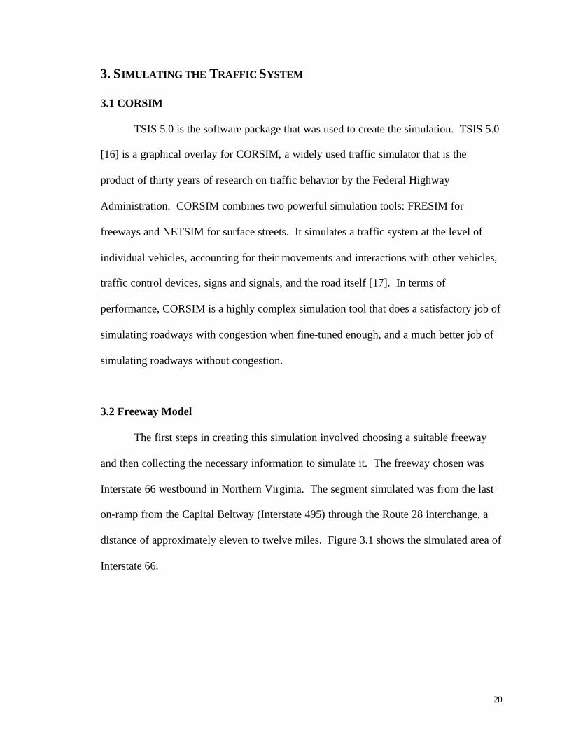
3.2 Freeway Model

The first steps in creating this simulation involved choosing a suitable freeway

and then collecting the necessary information to simulate it. The freeway chosen was

Interstate 66 westbound in Northern Virginia. The segment simulated was from the last

on-ramp from the Capital Beltway (Interstate 495) through the Route 28 interchange, a

distance of approximately eleven to twelve miles. Figure 3.1 shows the simulated area of

Interstate 66.

21

Figure 3.1 - Simulated Segment of Interstate 66 [18](Segment highlighted in blue)

Interstate 66 was chosen because it is a heavily congested freeway corridor,

representative of many of the roads in the Northern Virginia area during rush hour. The

segment chosen is relatively uniform in design, with three regular lanes and one HOV

lane during peak-hour traffic. It is also the most congested segment of the freeway

westbound (or outside) of the Capital Beltway. Both the simulation data and the raw data

collected from the freeway confirm this. I chose the westbound direction over the

eastbound because it was the direction for which peak-hour data was available.

A Northern Virginia roadmap from ADC [5] provided most of the structural

information about the road, such as distances between entrances and exits and a general

idea of the layout of Interstate 66. The Smart Travel Lab provided the volume

information needed to populate and validate the system. This data also provided more

information about the structure of the road, such as lane counts and layout information.

When neither of these two sources could answer a question about the freeway, road maps

or aerial photographs available on the web from MapQuest [6] provided the additional

information.

Hundreds of detectors placed throughout Interstate 66 supplied the volume data

provided by the Smart Travel Lab. The specific data used to populate the simulation was

collected from detectors between 6 and 7 p.m. on February 21, 2002. Volumes were

22

provided for the freeway itself and numerous off-ramps and on-ramps. The data was not

100% comprehensive, however, and therefore volume estimates had to be made for one

segment of the freeway in the Route 50 interchange, a lane of the freeway in the Route

123 interchange, the off-ramp for Route 28 northbound, and the HOV off-ramp for

Monument Drive. Since none of these values was needed as entry node data for the

freeway simulation, however, these data holes were only an issue in the validation of the

simulation, and not an issue in its creation.

3.3 Simulating Interstate 66

Once the necessary information was collected and organized, the simulation was

created in TSIS 5.0 [16]. I created the infrastructure first and then populated it with the

volume information. TSIS 5.0 required on-ramp and freeway entry data to be provided as

a vehicles per hour flow, but off-ramp data needed to be provided as a percentage of total

flow through that segment of the freeway. This becomes important during the validation

process, since any deviation of simulated volumes from actual volumes in a segment of

the freeway would create proportional deviations from actual volumes at the off-ramps.

This, in turn, would magnify and propagate these inaccuracies to further segments of the

freeway.

I obtained defaults from the Highway Capacity Manual [19] for some information

that was not provided by any source. These defaults included acceleration lanes of 600

feet, deceleration lanes of 150 ft, and a relative volume of 5% trucks and heavy vehicles.

An approximate percentage of 10% was calculated from the Smart Travel Lab data for

the relative number of high occupancy vehicles (those that could use HOV lanes) on the

23

road at any given time. Lastly, I gave drivers an average free-flow speed of 65 mph, and

a range of free-flow speeds between approximately 55 and 75 mph. Although the speed

limit on this segment of Interstate 66 is 55 mph, data from the Smart Travel Lab and

personal experience on the road showed a range of speeds closer to that used in the

simulation.

The simulation was validated by comparing hourly vehicle volumes generated by

the simulation to the actual hourly volumes from the Smart Travel Lab data. I compared

simulation and actual data from the on-ramps, off-ramps, and freeway segments. Overall,

the simulation volumes were relatively consistent with the data provided from the Smart

Travel Lab. Figure 3.2 compares the simulation and actual vehicle volumes for all

freeway segments for which reasonably complete data was available. Refer to Appendix

A for a numerical comparison of actual and simulation volumes, including on-ramp and

off-ramp volumes accompanied by additional freeway data.

0

100020003000400050006000

700080009000

[I-49

5, I-4

95]

[I-49

5, R

t. 24

3][R

t. 24

3, R

t. 24

3][R

t. 24

3, R

t. 12

3][R

t. 12

3, R

t. 12

3][R

t. 12

3, R

t. 50

][R

t. 50

, Rt.

50]

[Rt.

50, R

t. 50

][R

t. 50

, Mon

. Dr.]

[Mon

. Dr.,

Rt.

7100

][R

t. 71

00, R

t. 71

00]

[Rt.

7100

, Str.

Rd.

][S

tr. R

d., R

t. 28

][R

t. 28

, Rt.

28]

[Rt.

28, R

t. 28

][R

t. 28

, Rt.

29]

Num

ber o

f Veh

icle

s

Actual Simulated Entry Backup

Figure 3.2 - Comparison of Simulated and Actual Vehicle Volumes(Freeway segments shown in order as [Prev. Route, Next Route] pairs)

24

The largest problems occurred because of vehicle backup behind the entry points

of the simulation. Approximately 2,400 vehicles programmed to enter the simulation

during the hour never made it into the freeway from the freeway entry point (hence the

entry backup on the first freeway segment shown in Figure 3.2) and several on-ramps

near the beginning of the simulated roadway segment. This number was originally higher

but alleviated with extensive manipulation of simulation parameters, including use of the

default information described earlier. This created queues of vehicles at some entry

points that were waiting to enter the freeway due to a lack of physical road space. This

failure of 2,400 vehicles to enter the freeway prevented accurate flow readouts from

many areas of the freeway and off-ramps. Later in the simulation, the on-ramp data are

more accurate, since zero vehicles backed up behind the on-ramp entry points. However,

the freeway data are about 1,500 to 2,000 vehicles fewer than it should be in all areas,

due to the congestion issues at the beginning of the simulation. Additionally, the off-

ramp readings are somewhat lower, due to the need to provide off-ramp data as a

percentage of total flow through a segment of the freeway, as mentioned earlier.

One reason for these vehicle backups behind the entry points probably has to do

with the aggressiveness level of drivers in the simulation. It is likely that the actual

drivers on Interstate 66 are considerably more aggressive with both road entry maneuvers

and following distances. The CORSIM simulator places vehicles with a number of

different driving behaviors on the road - a driver has the same chance of being overly

cautious as overly aggressive. After an exhaustive search of the program, it is my

conclusion, unfortunately, that the frequency of aggressive drivers cannot be adjusted in

the CORSIM model, and I was therefore forced to keep this bell curve distribution of

25

driving behaviors. In contrast, Interstate 66 has considerably more aggressive drivers

than careful ones, based on my personal experience driving the road, meaning closer

following distances and more aggressive actions to enter the freeway. These two factors

would lead to increased freeway volume and greater congestion.

Additionally, CORSIM tends to project a pessimistic view of driver behavior

when it comes to lane changes. CORSIM drivers do not like to let vehicles into their lane

if their following distance will be violated. In real life, violation of a driver's following

distance is usually the only way to enter the freeway in such a congestion situation. This

could therefore be partially responsible for the large queues of waiting vehicles.

Regardless of these flaws, however, I chose to use this simulation to perform the

experiments, as it still does a reasonably good job of representing this freeway.

Furthermore, it still models a very realistic freeway scenario, which is what is most

important for the purposes of these experiments. This simulation gave me the control

data that I needed to make comparisons. The control data are better to use for

comparisons than the actual data, as all of it was obtained in the same environment from

which the experimental data was obtained. This allows one to see clearly the effects of

the experiments that were performed. Additionally, the actual data contains a significant

amount of measurement error that would skew any conclusions that one attempted to

draw from comparison after completion of the experiments.

26

4. EXPERIMENTATION

4.1 Applying Each Technique

I applied each technique to the traffic system and then compared it to the control

data in a number of different areas, including calculated on-ramp wait times and total

travel time through the freeway segment. The data included volumes at specific parts of

the freeway, including on-ramps and off-ramps, travel times through freeway segments,

and backups of vehicles behind entry points and on-ramps in the simulation. Although

measuring the flow directly does not tell us much, we indirectly get a sense of the number

of vehicles that the freeway services during the simulated hour of operation through the

numbers of vehicles queued behind the entry points. For example, the simulation without

any congestion control techniques allowed 12,438 vehicles to enter out of 14,838 wanting

to use the freeway during that hour, about an 84% service rate.

Most of the techniques applied to the simulation were modified to be considerably

more predictable and predetermined than they usually are in data networks. I did this for

reasons discussed in the section comparing data networks and traffic systems, and

because the simulation software required each technique to be pigeon-holed into one of

five ramp metering techniques. Consequently, I used a multiple threshold occupancy

meter, calibrated with the philosophy of the congestion control scheme in mind, to apply

most of the techniques.

Additionally, techniques that used multiple threshold occupancy metering only

metered three of the on-ramps in the simulation - the rest remained unmetered. The

primary reason for this was that the simulation software had internal problems with

implementing more than about three multiple threshold occupancy on-ramp meters.

27

Practically, however, this was enough, since traffic-slowing congestion only occurred in

the first segments of the simulation, where these on-ramp meters were placed. Since the

later segments approached free-flow speed, it made no sense to meter downstream on-

ramps. Such metering would cause queue buildup at those on-ramps with no added

benefit.

Table 4.1 lists the descriptions of the implementation algorithms for applying

each of the techniques to the simulation, with more detailed information available in

Appendix B.

Congestion Control Algorithm Algorithm DescriptionEthernet Applied 1-persistence congestion control with no exponential back-off.

Metered at maximum rate if no congestion, else minimum rate.Used Multiple Threshold Occupancy Meter.

AIMD Allowed one extra vehicle per minute as congestion lessened. Duringcongestion, metering rate was halved as congestion got worse.Used Multiple Threshold Occupancy Meter.

Slow-Start Doubled metering rate when congestion lessened, halved whencongestion worsened. Prevented "burst" with an even metering rate forlow and moderate congestion levels. (Simple implementation.)Used Multiple Threshold Occupancy Meter.

TCP Vegas Defined occupancy thresholds for too little and too much traffic on thefreeway, increased ramp-metering rate below minimum threshold, anddecreased it above maximum threshold.Used Multiple Threshold Occupancy Meter.

DECbit Decreased metering rate by one-eighth as congestion worsened.Used Multiple Threshold Occupancy Meter.

Friendly Rate Control Increased metering a little as congestion lightened; dropped to thresholdvalue when congestion increased, and held that rate even if congestiongot worse. Never reacted harshly to excess capacity/congestion.Used Multiple Threshold Occupancy Meter.

RED Metered at maximum rate if no congestion, else lowered rate ascongestion got worse, and metered at minimum rate at a certain threshold.Used Multiple Threshold Occupancy Meter.

Fair Queueing/WFQ Metered all on-ramps at the same rate ("fairly"). Weighted meteringapplied for a WFQ system, to allow proportionally more vehicles fromon-ramps that were more popular.Used clock-time metering.

Lane Added Added an additional lane to this segment of Interstate 66 to increase thecapacity on the freeway where it was needed most.

Table 4.1 - Procedures for Applying Congestion Control Techniques

28

As an example of how I cross-applied techniques, and to help with understanding

the table, we can consider the implementation algorithm for DECbit. DECbit was

described earlier as a technique that marked packets to determine congestion, and

decreased the sending rate by one-eighth while congestion persisted, or increased the rate

linearly when below a certain congestion threshold. In applying this technique to the

freeway system, I chose to use a multiple threshold occupancy meter. Since the detectors

in the roadway could give us a much better idea of how much congestion existed than the

estimation used in the real DECbit algorithm, I chose to adapt the technique to the

detector information. The resulting implementation algorithm was considerably more

deterministic than the real DECbit congestion control scheme, as was the case with every

technique modified for the simulation. Rather than decreasing the metering rate by one-

eighth while congestion persisted, I decided to decrease the metering rate as congestion

got progressively worse, as defined by a number of occupancy thresholds. The baseline

for the technique was the maximum metering rate (15 vehicles/minute/on-ramp lane) and

zero percent occupancy. Whenever congestion worsened and exceeded an occupancy

threshold, the current metering rate decreased by one-eighth. There was no linear

increase for congestion resolution, but the metering rate was allowed to increase again

when congestion dropped below a threshold.

4.2 Experimental Results

The results show us almost immediately that some congestion control techniques

fail miserably at their task, generally because of tremendously unreasonable on-ramp wait

times. As was hinted earlier, the techniques that dramatically reduce flow in response to

29

congestion were some of the worst to fare in the experiment, producing on-ramp wait

times of up to, in the most extreme case, fifteen hours. Deploying such techniques would

likely lead to a level of road rage far worse than any benefits produced from improved

travel times or throughput. The following figures summarize the results of the

experiment. Figure 4.1 shows travel time for the entire freeway segment, not including

on-ramp wait or entry times, for each congestion control technique. Figure 4.2 shows

throughput for the techniques, measured in number of vehicles that were able to enter the

freeway at that hour. Finally, Figure 4.3 gives us the average on-ramp wait times of all

metered on-ramps for each technique. All techniques are compared to the control

simulation and free-flow conditions. Free-flow means that vehicles always travel the

freeway at 65 mph, with nothing impeding their speed, and that all vehicles wanting to

enter the freeway are allowed to do so immediately. In other words, free-flow indicates a

freeway with infinite traffic capacity and no delay time. Appendices C and D contain

further results from these experiments.

30

0

5

10

15

20

25

Con

trol

Ethe

rnet

AIM

D

Slow

Sta

rt

TCP

Vega

s

DECb

it

FRC

RED

Fair

Que

uein

g

WFQ

Lane

Add

ed

Free

-Flo

wAve

rag

e T

rave

l Tim

e (m

inu

tes)

Figure 4.1 - Freeway Travel Times for Each Technique

02000400060008000

10000120001400016000

Con

trol

Ethe

rnet

AIM

D

Slow

Sta

rt

TCP

Vega

s

DECb

it

FRC

RED

Fair

Que

uein

g

WFQ

Lane

Add

ed

Free

-Flo

w

Th

rou

gh

pu

t (v

ehic

les/

ho

ur)

Figure 4.2 - Throughput for Each Technique

1

10

100

1000

Con

trol

Ethe

rnet

AIM

D

Slow

Sta

rt

TCP

Vega

s

DECb

it

FRC

RED

Fair

Que

uein

g

WFQ

Lane

Add

ed

Free

-Flo

w

Wai

t T

ime

(min

ute

s)

Figure 4.3 - Average On-Ramp Wait Times for Each Technique(Lane Added & Free-Flow Wait Times were less than one minute)

31

A successful technique achieves a balance between travel time, throughput, and

on-ramp waiting times. Many techniques, such as Ethernet, AIMD, and RED, achieved

good travel times, but their on-ramp waiting times were very high. Other techniques,

such as Weighted Fair Queueing, did an okay job of balancing on-ramp wait times and

travel times, but at the expense of a considerably decreased throughput. All of the ramp

metering techniques had a decrease in throughput from the control, since they alleviated

congestion on the freeway by moderating vehicle entry at on-ramps, thereby allowing

fewer vehicles to use the freeway during the hour.

Overall, it would appear that none of the simulation techniques performed

tremendously well except for adding a lane, which had a significant improvement in all

areas. Unfortunately, all that really shows is that adding a lane to a freeway improves

flow, capacity, and travel times, which is not an interesting or particularly relevant

conclusion for this project. Adding a lane, however, does reduce congestion to a level at

which the techniques may become more useful. The techniques that appear to have the

most promising results, if fine-tuned and applied alongside the addition of an extra

freeway lane, are DECbit, Friendly Rate Control, and Fair Queueing. The combination

and fine-tuning of techniques to achieve maximum positive effects are the focus of the

next chapter.

32

5. PRAGMATIC TECHNIQUE APPLICATION

5.1 Combining and Fine-tuning Successful Techniques

The results indicated that adding a lane to the freeway simulation increased the

capacity of the road, provided lower travel times and entry wait times, and increased

throughput. This chapter will demonstrate the ability of DECbit and fine-tuned versions

of Fair Queueing and Friendly Rate Control, combined with the addition of a lane to the

freeway, to have a considerable effect on freeway performance. Adding a lane reduces

congestion and increases the success of the techniques, as most techniques were

unsuccessful where the traffic network was overloaded. Often, combining the addition of

a lane with these techniques improved travel times and throughputs while cutting average

on-ramp waiting times by as much as half. The techniques were generally fine-tuned by

increasing their average metering rates in order to take advantage of the newly available

lane capacity.

As a series of follow up experiments, the addition of a lane was first combined

with the DECbit technique. DECbit was unmodified before combination, as any

modification would either reduce the metering rates or compromise the accurate

emulation of the DECbit algorithm. The next experiment was to combine the addition of

a lane with a fine-tuned version of Friendly Rate Control with a slightly higher average

metering rate. Next, Friendly Rate Control was fine-tuned even further to supply the

highest average metering rate possible while still emulating the algorithm accurately.

Finally, Fair Queueing was implemented on the three on-ramps to which most of the

congestion control techniques were exclusively applied. This would eliminate the issue

of queue buildup on areas of the freeway where metering did not provide any noticeable

33

benefits. Additionally, the metering rate was increased to the maximum rate possible (15

vehicles per minute), again to maximize use of freeway capacity. Lastly, this technique

was also combined with the addition of a lane to the freeway. Appendix B contains more

information on these follow-up experiments.

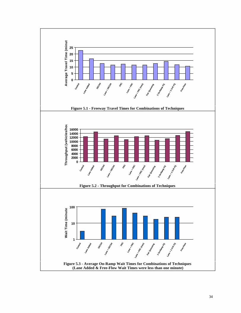
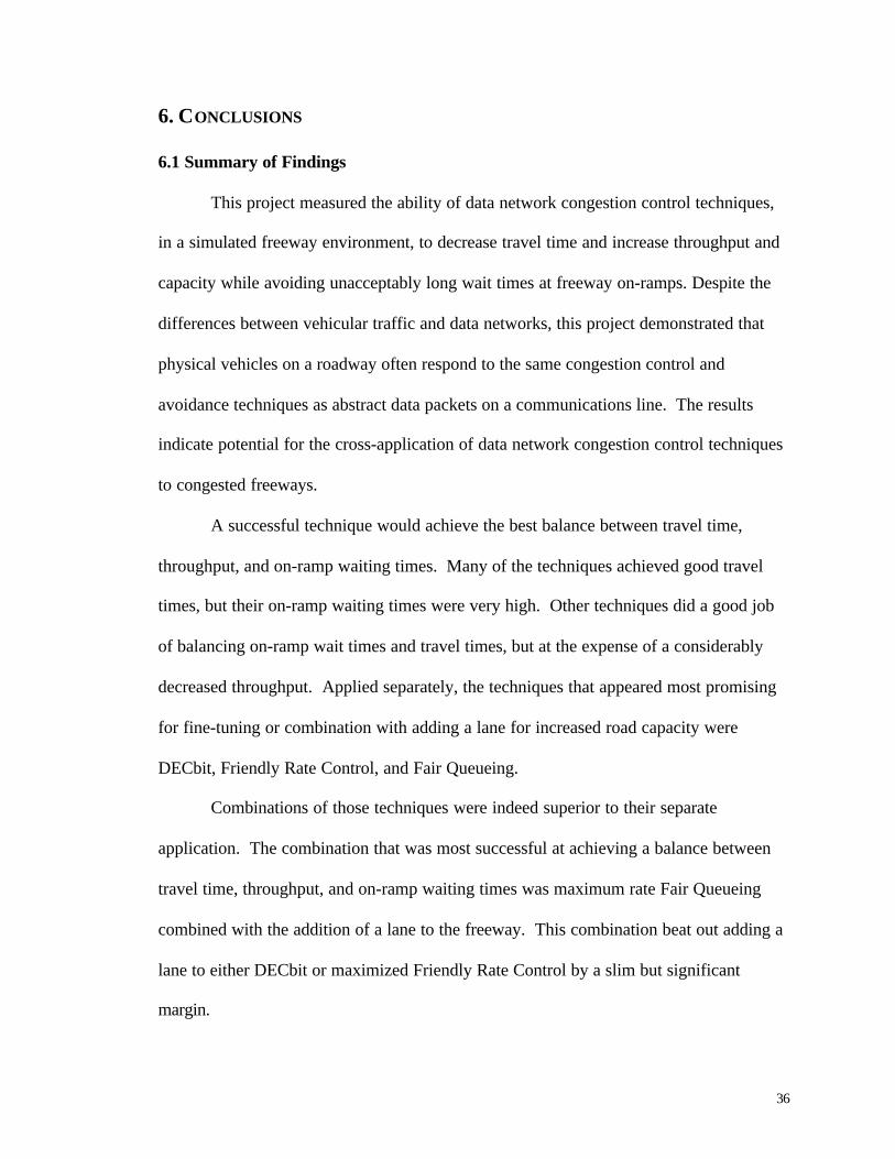
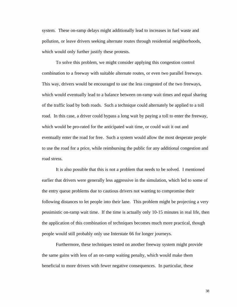
The following figures summarize the results of these experiments and compare

the effectiveness of the combinations with their separate application. Figure 5.1 shows

travel time for the entire freeway segment, not including on-ramp wait or entry times, for

each set of techniques. Figure 5.2 shows throughput for each set of techniques, measured

in number of vehicles that were able to enter the freeway at that hour. Finally, Figure 5.3

gives us the average on-ramp wait times of all metered on-ramps for each set of

techniques. All sets of techniques are compared to the control simulation and free-flow

conditions. Appendices C and D contain further results from these experiments.

34

0

5

10

15

20

25

Cont

rol

Lane

Add

ed

DECb

it

Lane

+ D

ECbi

t

FRC

Lane

+ F

RCLa

ne +

FRC

(max

)

Fair

Que

uein

g

3 On

-Ram

p FQ

Lane

+ 3

O-R

FQ

Free

-Flo

wAve

rag

e T

rave

l Tim

e (m

inu

tes)

Figure 5.1 - Freeway Travel Times for Combinations of Techniques

02000400060008000

10000120001400016000

Cont

rol

Lane

Add

ed

DECb

it

Lane

+ D

ECbi

t

FRC

Lane

+ F

RCLa

ne +

FRC

(max

)

Fair

Que

uein

g

3 On

-Ram

p FQ

Lane

+ 3

O-R

FQ

Free

-Flo

w

Th

rou

gh

pu

t (v

ehic

les/

ho

ur)

Figure 5.2 - Throughput for Combinations of Techniques

1

10

100

Cont

rol

Lane

Add

ed

DECb

it

Lane

+ D

ECbi

t

FRC

Lane

+ F

RCLa

ne +

FRC

(max

)

Fair

Que

uein

g

3 On

-Ram

p FQ

Lane

+ 3

O-R

FQ

Free

-Flo

w

Wai

t T

ime

(min

ute

s)

Figure 5.3 - Average On-Ramp Wait Times for Combinations of Techniques(Lane Added & Free-Flow Wait Times were less than one minute)

35

One could conclude from the figures that these improved techniques on a less

overloaded freeway were superior to their earlier application. Overall, it appears that

maximum rate Fair Queueing combined with the addition of a lane was most successful

at achieving a balance between travel time, throughput, and on-ramp waiting times.

DECbit and maximized Friendly Rate Control were close, when given an additional lane,

but did not achieve the balance as well. Comparing the three techniques, Fair Queueing

had a slightly greater freeway travel time, but a significantly greater throughput of about

200 vehicles, and an average metered on-ramp wait time of about five minutes less.

5.2 Evaluation of Most Successful Combination

Luckily, the most successful combination of techniques is also a rather easy one

to apply in real life. Three on-ramp meters would be placed at the final Interstate 495 on-

ramp as well as the Nutley Street on-ramp and the second Route 123 on-ramp. These on-

ramp meters are simply clock-time ramp meters with a headway of four seconds. The

more costly part of this project would be the addition of an extra lane to this segment of

Interstate 66. Since Fair Queueing on three on-ramps actually performs reasonably well

on its own, however, it is possible to start the metering signals before finishing the road

widening project in order to benefit from them as early as possible. This road

improvement project would literally cut travel times along this segment in half and

increase throughput by approximately 600 vehicles, at the cost of a 20-25 minute wait on

three of the entry on-ramps. Such a wait, unfortunately, would not be accepted by the

public. The wait time at these on-ramps is simply too long for the drivers to benefit from

the improvement in travel times on the actual freeway.

36

6. CONCLUSIONS

6.1 Summary of Findings

This project measured the ability of data network congestion control techniques,

in a simulated freeway environment, to decrease travel time and increase throughput and

capacity while avoiding unacceptably long wait times at freeway on-ramps. Despite the

differences between vehicular traffic and data networks, this project demonstrated that

physical vehicles on a roadway often respond to the same congestion control and

avoidance techniques as abstract data packets on a communications line. The results

indicate potential for the cross-application of data network congestion control techniques

to congested freeways.

A successful technique would achieve the best balance between travel time,

throughput, and on-ramp waiting times. Many of the techniques achieved good travel

times, but their on-ramp waiting times were very high. Other techniques did a good job

of balancing on-ramp wait times and travel times, but at the expense of a considerably

decreased throughput. Applied separately, the techniques that appeared most promising

for fine-tuning or combination with adding a lane for increased road capacity were

DECbit, Friendly Rate Control, and Fair Queueing.

Combinations of those techniques were indeed superior to their separate

application. The combination that was most successful at achieving a balance between

travel time, throughput, and on-ramp waiting times was maximum rate Fair Queueing

combined with the addition of a lane to the freeway. This combination beat out adding a

lane to either DECbit or maximized Friendly Rate Control by a slim but significant

margin.

37

One obvious reason that this combination was successful is that adding a lane

increases the capacity of the freeway, which automatically lightens congestion and makes

most of the other techniques more effective. Furthermore, I mentioned earlier that ramp

metering techniques that respond too drastically to an increase or decrease in congestion

tend to fare much worse than those that respond more gradually. Clients on a network

can be expected to put up with the occasional unreasonable delay - drivers usually

cannot. In fact, it appears that in freeway systems, often it is best not to modify the

metering rate at all, but instead to program the ramp meter with a constant headway that

fully uses available capacity without causing congestion. Certainly, this proved to be the

best balancing technique in this sequence of experiments. Perhaps, however, a correctly

calibrated adaptive metering technique would prove more effective in another

experimental sequence.

6.2 Discussion and Interpretation of Results

The most promising combination to apply to a freeway for the greatest positive

net effect is maximized Fair Queueing combined with the addition of a lane to the

freeway. This combination would provide a significant decrease in freeway travel time

and increase in throughput. However, it would also provide a significant wait at certain

on-ramps of nearly 20-25 minutes. This is a 15-20 minute increase from the wait before

applying any congestion control techniques. Would such a wait be a problem? This

depends on the magnitude of the decrease in freeway travel time, but it is likely that it

would not be acceptable to the driving public. Unreasonable on-ramp delays might lead

to an ignorance or avoidance of the system, or protests from drivers to shut down the

38

system. These on-ramp delays might additionally lead to increases in fuel waste and

pollution, or leave drivers seeking alternate routes through residential neighborhoods,

which would only further justify these protests.

To solve this problem, we might consider applying this congestion control

combination to a freeway with suitable alternate routes, or even two parallel freeways.

This way, drivers would be encouraged to use the less congested of the two freeways,

which would eventually lead to a balance between on-ramp wait times and equal sharing

of the traffic load by both roads. Such a technique could alternately be applied to a toll

road. In this case, a driver could bypass a long wait by paying a toll to enter the freeway,

which would be pro-rated for the anticipated wait time, or could wait it out and

eventually enter the road for free. Such a system would allow the most desperate people

to use the road for a price, while reimbursing the public for any additional congestion and

road stress.

It is also possible that this is not a problem that needs to be solved. I mentioned

earlier that drivers were generally less aggressive in the simulation, which led to some of

the entry queue problems due to cautious drivers not wanting to compromise their

following distances to let people into their lane. This problem might be projecting a very

pessimistic on-ramp wait time. If the time is actually only 10-15 minutes in real life, then

the application of this combination of techniques becomes much more practical, though

people would still probably only use Interstate 66 for longer journeys.

Furthermore, these techniques tested on another freeway system might provide

the same gains with less of an on-ramp waiting penalty, which would make them

beneficial to more drivers with fewer negative consequences. In particular, these

39

techniques might have a greater likelihood of working on a freeway with less congestion.

The segment of Interstate 66 that I simulated is located in a heavily congested area of

Northern Virginia, which has traffic congestion problems comparable to the New York

City and Los Angeles metropolitan areas. It is quite likely that these three regions have

the largest traffic congestion problems in the nation. Applying these techniques to a less

problematic road might work a lot better.

We must also keep in mind that any action taken to improve the flow of a road

will probably lead to increased confidence in that road and therefore a possible

resurgence of higher travel times and longer on-ramp waits. This is an unavoidable side

effect of trying to improve any roadway, and its resolution is beyond the scope of this

project. It should also be noted that this system would do nothing to improve freeways

that are congested due to roadway incidents such as accidents. Therefore, if application

of these techniques results in higher incident levels on the freeway, this might be a reason

for discontinuing their use. In conclusion, Fair Queueing combined with the addition of a

lane is the combination recommended for practical application by this report, as it

provides numerous benefits to drivers while keeping the added burdens to a minimum.

6.3 Recommendations for Future Research

This project presents numerous opportunities for future research. One could

choose a different road to simulate and perform the same experiments on that simulation.

It is quite possible that applying these techniques to a less congested road would be much

more effective. Alternately, one could choose to apply these techniques to the same

segment of I-66 with a different application strategy.

40

There are also other research possibilities, given the advancements in the fields of

traffic engineering and data networks. A newer, more centralized and deterministic

congestion control technique that adapts itself better to traffic systems may be invented.

Additionally, networks that are or become more centralized, and can use detectors of

some sort to provide more definitive measurements of congestion, might benefit from the

application of ramp metering techniques, as they would avoid unnecessary guesswork

and provide a cleaner solution to congestion resolution for that network. Alternatively,

freeway systems that are more decentralized might benefit from applying one of the data

network congestion control techniques outlined in this report.

6.4 Report Summary

This project demonstrated the potential for the cross-application of data network

congestion control techniques to congested freeways. The techniques that appeared most

promising, when applied separately, for fine-tuning or combination were DECbit,

Friendly Rate Control, and Fair Queueing. When techniques were combined and fine-

tuned, the combination that was most successful at achieving a balance between travel

time, throughput, and on-ramp waiting times was Fair Queueing at the most congested

on-ramps combined with the addition of a lane to the freeway. Some reasons why this

combination was successful were that adding a lane increases the capacity of the freeway,

and that ramp metering techniques fare better when they respond less radically to

congestion.

While this combination would provide a significant decrease in freeway travel

time and increase in throughput, it would also require a significant wait at certain on-

41

ramps of nearly 20-25 minutes. This wait would likely be a problem in a real-world

implementation. Some solutions to this wait problem include alternate routes, parallel

freeways, and toll roads pro-rated for current wait time. It is also possible that this wait

time problem results from a pessimistic simulation tool or unmanageable levels of

congestion on this particular freeway.

This project creates several opportunities for additional research, including

modifying the technique application strategies or the freeway on which the experiments

are performed. Advancements might lead to other possibilities for research, including

application of new techniques or more practical cross-applications of techniques.

Ultimately, this paper hopes to encourage the sharing of information between two

similar areas of research - data network and freeway system congestion resolution. Such

sharing might not only uncover new ways to reduce congestion in both systems, but

might also allow both systems to identify and correct their flaws by using the alternate

system as a successful model when appropriate.

42

WORKS CITED

[1] N. Levy, M. Bragman. Bumper to Bumper: Transportation SystemsManagement…. New York: The Legislative Commission on CriticalTransportation Choices, 1989.

[2] R. Herman, K. Gardels. Vehicular Traffic Flow. Scientific American. p. 35-43.December 1963.

[3] Defense Advanced Research Projects Agency. RFC 793, Transmission ControlProtocol: DARPA Internet Program Protocol Specification, September 1981.

[4] L. Peterson, B. Davie. Computer Networks: A Systems Approach. San Diego: TheAcademic Press, 2000.

[5] ADC The Map People. Regional Northern Virginia: The Original Street MapBook. Alexandria, VA: Langenscheidt Publishing Group, 2001.

[6] MapQuest.com, Inc. MapQuest, 2002. http://www.mapquest.com.

[7] Jacobson, V., J. Karels. Congestion Avoidance and Control. In Proceedings ofSIGCOMM '88 (Stanford, CA, Aug. 1988), ACM.

[8] S. Floyd, M. Handley, J. Padhye, J. Widmer. Equation-Based Congestion Controlfor Unicast Applications. In Proceedings of SIGCOMM '00 (Stockholm, Sweden,July 2000), ACM.

[9] S. Floyd, V. Jacobson. Random Early Detection Gateways for CongestionAvoidance. In IEEE/ACM Transactions on Networking, August 1993.

[10] I. Stoica, S. Shenker, H. Zhang. Core-Stateless Fair Queueing: AchievingApproximately Fair Bandwidth Allocations in High Speed Networks. InProceedings of SIGCOMM '98 (Vancouver, British Columbia, September 1998),ACM.

[11] V. Padmanabhan, L. Qiu. The Content and Access Dynamics of a Busy Web Site:Findings and Implications. In Proceedings of SIGCOMM '00 (Stockholm,Sweden, July 2000), ACM.

[12] New York State Department of Transportation. LI ITS Benefits, March 2002.http://www.dot.state.ny.us/reg/r10/benefits.html.

[13] U.S. Department of Transportation, Federal Highway Administration. Manual onUniform Traffic Control Devices (MUTCD), June 2001.http://mutcd.fhwa.dot.gov/kno-millennium_06.14.01.htm. Sections 4H.01 and4H.02.

43

[14] J. Liu, J. Kim. An Advanced Real-Time Ramp Metering System (ARMS): TheSystem Concept. Research Report (College Station, TX, November 1994), TexasTransportation Institute.

[15] M. Zhang, T. Kim, X. Nie, W. Jim. Evaluation of On-Ramp Control Algorithms.Research Report (Davis, CA, September 2001), Institute of Transportation Studiesat the University of California, Davis.

[16] FHWA Office of Operations Research, Development, and Technology. TSIS 5.0.Washington, D. C.: ITT Industries Inc., Systems Division, 2001.

[17] New York State Department of Transportation. New York Route 347 CORSIMSReference Page, 2000. http://www.ny347.com/CORSIM.htm.

[18] DeLorme. Virginia Atlas & Gazetteer. Yarmouth, MA: DeLorme, 2000.

[19] Transportation Research Board, National Research Council. Highway CapacityManual (HCM 2000). Washington, D. C.: The National Academy of Sciences,2000.

44

BIBLIOGRAPHY

ADC The Map People. Regional Northern Virginia: The Original Street Map Book.Alexandria, VA: Langenscheidt Publishing Group, 2001.

Breslau, L., E. Knightly, S. Shenker, I. Stoica, H. Zhang. Endpoint Admission Control:Architectural Issues and Performance. In Proceedings of SIGCOMM '00(Stockholm, Sweden, July 2000), ACM.

Byers, J., M. Frumin, G. Horn, M. Luby, M. Mitzenmacher, A. Roetter, W. Shaver.FLID-DL: Congestion Control for Layered Multicast. In Proceedings of NGC '00(Palo Alto, CA, November 2000), ACM.

Defense Advanced Research Projects Agency. RFC 793, Transmission ControlProtocol: DARPA Internet Program Protocol Specification, September 1981.

DeLorme. Virginia Atlas & Gazetteer. Yarmouth, MA: DeLorme, 2000.

Evans, D. Programming the Swarm. Department of Computer Science (Charlottesville,VA, July 2000), University of Virginia.

Feldmann, A., A. Greenberg, C. Lund, N. Reingold, J. Rexford, F. True. DerivingTraffic Methods for Operational IP Networks: Methodology and Experience. InProceedings of SIGCOMM '00 (Stockholm, Sweden, July 2000), ACM.

FHWA Office of Operations Research, Development, and Technology. TSIS 5.0.Washington, D. C.: ITT Industries Inc., Systems Division, 2001.

Floyd, S., V. Jacobson. Random Early Detection Gateways for Congestion Avoidance.In IEEE/ACM Transactions on Networking, August 1993.

Floyd, S., M. Handley, J. Padhye, J. Widmer. Equation-Based Congestion Control forUnicast Applications. In Proceedings of SIGCOMM '00 (Stockholm, Sweden,July 2000), ACM.

Herman, R., K. Gardels. Vehicular Traffic Flow. Scientific American. p. 35-43.December 1963.

Jacobson, V., J. Karels. Congestion Avoidance and Control. In Proceedings ofSIGCOMM '88 (Stanford, CA, Aug. 1988), ACM.

Levy, N., M. Bragman. Bumper to Bumper: Transportation Systems Management….New York: The Legislative Commission on Critical Transportation Choices,1989.

45

Liu, J., J. Kim. An Advanced Real-Time Ramp Metering System (ARMS): The SystemConcept. Research Report (College Station, TX, November 1994), TexasTransportation Institute.

MapQuest.com, Inc. MapQuest, 2002. http://www.mapquest.com.

New York State Department of Transportation. LI ITS Benefits, March 2002.http://www.dot.state.ny.us/reg/r10/benefits.html.

New York State Department of Transportation. New York Route 347 CORSIMSReference Page, 2000. http://www.ny347.com/CORSIM.htm.

Padmanabhan, V., L. Qiu. The Content and Access Dynamics of a Busy Web Site:Findings and Implications. In Proceedings of SIGCOMM '00 (Stockholm,Sweden, July 2000), ACM.

Peterson, L., B. Davie. Computer Networks: A Systems Approach. San Diego: TheAcademic Press, 2000.

Resnick, M. Turtles, Termites, and Traffic Jams. Cambridge: The MIT Press, 2000.

Stoica, I., S. Shenker, H. Zhang. Core-Stateless Fair Queueing: AchievingApproximately Fair Bandwidth Allocations in High Speed Networks. InProceedings of SIGCOMM '98 (Vancouver, British Columbia, September 1998),ACM.

Stoica, I., H. Zhang. Providing Guaranteed Services Without Per Flow Management. InProceedings of SIGCOMM '99 (Cambridge, MA, August 1999), ACM.

Thorpe, T. A Physically-Realistic Simulation of Vehicle Traffic Flow. Computer ScienceTechnical Report (Fort Collins, CO, January 1998), Colorado State University.

Transportation Research Board, National Research Council. Highway Capacity Manual(HCM 2000). Washington, D. C.: The National Academy of Sciences, 2000.

U.S. Department of Transportation, Federal Highway Administration. Manual onUniform Traffic Control Devices (MUTCD), June 2001.http://mutcd.fhwa.dot.gov/kno-millennium_06.14.01.htm. Sections 4H.01 and4H.02.

Zhang, M., T. Kim, X. Nie, W. Jim. Evaluation of On-Ramp Control Algorithms.Research Report (Davis, CA, September 2001), Institute of Transportation Studiesat the University of California, Davis.

46

APPENDICES

Appendix A: Simulation Verification Data

February 21, 2002: 6PM Actual Data and Simulation Output for Segment of I-66LnTyp PRN NRN TotLn Actual

VolumeSimul.Volume

EntryBackup

SimulatedMin/Mile

SegmentLength (ft)

TravelTime (min)

Actual% Occ.

Norm Rt 28 Rt 29 5 5694 3696 0.97 750 0.14 7.44 Before Rt. 29On Rt 28 Rt 28 1 1133 1132 0 0.96 10.62 Onramp from Rt. 28

Norm Rt 28 Rt 28 4 4529 2571 0.96 568 0.10 7.38 Rt. 28 InterchangeOff Rt 28 Rt 28 1 984 442 0.96 9.15 Rt. 28 Offramp #2

Norm Rt7100

Rt 28 4 6357 3030 0.96 1563 0.28 10.80 Before Rt. 28

Off Rt 28 Rt 28 1 ~1391 562 1.00 --- Rt. 28 Offramp #1Norm Rt

7100Rt 28 4 6401 3678 0.97 7671 1.41 9.69 Before Rt. 28

HovOff Rt7100

Rt7100

1 177 191 0.97 1.33 Stringfellow Rd. Offramp (HOV)

Norm Rt7100

Rt7100

4 4750 3871 0.97 852 0.16 7.78 Rt. 7100 Interchange

On Rt7100

Rt7100

1 727 725 0 0.95 5.40 Onramp from Rt. 7100

Norm Rt7100

Rt7100

4 4904 3207 0.96 5398 0.98 7.53 Rt. 7100 Interchange

Off Rt7100

Rt7100

1 550 422 0.97 5.37 Rt. 7100 Offramp

Norm Rt7100

Rt7100

4 4936 3684 0.97 4688 0.86 8.17 Rt. 7100 Interchange

HovOff Rt 50 Rt7100

1 ~965 866 0.97 --- Monument Dr. Offramp (HOV)

Norm Rt 50 Rt7100

5 5901 4591 0.98 3125 0.58 7.81 Before Rt. 7100

On Rt 50 Rt 50 1 419 418 0 0.93 5.28 Onramp from Rt. 50 #2Norm Rt 50 Rt 50 4 5619 4183 0.98 994 0.18 9.73 Rt. 50 InterchangeOff Rt 50 Rt 50 1 216 235 0.97 3.05 Rt. 50 Offramp #2

Norm Rt 50 Rt 50 4 --- 4431 0.98 1421 0.26 --- Rt. 50 InterchangeOn Rt 50 Rt 50 1 434 434 0 0.93 4.58 Onramp from Rt. 50 #1

Norm Rt 50 Rt 50 4 5317 4013 0.97 1989 0.37 8.82 Rt. 50 InterchangeOff Rt 50 Rt 50 2 2273 1992 0.98 8.90 Rt. 50 Offramp #1

Norm Rt 123 Rt 50 5 7589 6126 1.34 6819 1.73 13.16 Before Rt. 50On Rt 123 Rt 123 1 1173 1171 0 0.96 14.85 Onramp from Rt. 123 #2

Norm Rt 123 Rt 123 4 4811 5089 4.30 1847 1.50 25.07 Rt. 123 InterchangeOn Rt 123 Rt 123 1 481 480 0 1.14 6.00 Onramp from Rt. 123 #1

Norm Rt 123 Rt 123 4 5856 4678 4.45 2131 1.80 23.87 Rt. 123 InterchangeOff Rt 123 Rt 123 2 596 539 1.42 2.07 Rt. 123 Offramp

Norm Rt 243 Rt 123 4 6512 5773 3.16 6393 3.83 21.21 Before Rt. 123On Rt 243 Rt 243 1 1555 1404 100 3.07 45.82 Onramp from Rt. 243

Norm Rt 243 Rt 243 4 6870 5003 3.56 7387 4.98 18.52 Rt. 243 InterchangeOff Rt 243 Rt 243 1 1702 1221 1.18 10.10 Rt. 243 Offramp

Norm Int495

Rt 243 4 8570 6550 2.24 7529 3.19 10.06 Before Rt. 243

On Int495

Int495

2 2526 2171 350 8.11 6.53 Onramp from I-495

Norm Int495

Int495

4 6390 4416 1950 7.57 300 0.43 7.70 I-495 Interchange

LnTyp = Lane Type, PRN = Previous Route Number, NRN = Next Route NumberTotLn = Total Lanes, Actual % Occ. = Actual Percent Occupancy

Table A.1 - Simulation Verification Data

47

Appendix B: Detailed Technique Application Procedures

Congestion Control Algorithm Algorithm DescriptionMTO Meter Settings Shown as [Metering Rate]([Occupancy Threshold]) Sets

Ethernet Applied 1-persistence congestion control with no exponential back-off.Metered at maximum rate if no congestion, else minimum rate.Used Multiple Threshold Occupancy Meter: 15(22%), 1(100%).Turned off meter during off-peak times.

AIMD Allowed one extra vehicle per minute as congestion lessened. Duringcongestion, metering rate was halved as congestion got worse.Used Multiple Threshold Occupancy Meter:15(5%), 14(10%), 13(15%), 12(22%), 6(35%), 3(100%).Turned off meter during off-peak times.

Slow-Start Doubled metering rate when congestion lessened, halved whencongestion worsened. Prevented "burst" with an even metering rate forlow and moderate congestion levels. (Simple implementation.)Used Multiple Threshold Occupancy Meter: 12(22%), 6(35%), 3(100%).Turned off meter during off-peak times.

TCP Vegas Defined occupancy thresholds for too little and too much traffic on thefreeway, increased ramp-metering rate below minimum threshold, anddecreased it above maximum threshold.Used Multiple Threshold Occupancy Meter: 15(15%), 8(35%), 1(100%).Turned off meter during off-peak times.

DECbit Decreased metering rate by one-eighth as congestion worsened.Used Multiple Threshold Occupancy Meter.15(15%), 13(20%), 11(25%), 9(30%), 7(35%), 6(100%).Not modified when an additional lane added.Turned off meter during off-peak times.

Friendly Rate Control Increased metering a little as congestion lightened; dropped to thresholdvalue when congestion increased, and held that rate even if congestiongot worse. Never reacted harshly to excess capacity/congestion.Used Multiple Threshold Occupancy Meter.10(10%), 9(15%), 8(22%), 7(100%)12(10%), 11(15%), 10(22%), 9(100%) [Combined with Added Lane]15(10%), 14(15%), 13(22%), 12(100%) [Max. + Comb. w/ Added Lane]Turned off meter during off-peak times.

RED Metered at maximum rate if no congestion, else lowered rate ascongestion got worse, and metered at minimum rate at a certain threshold.Used Multiple Threshold Occupancy Meter.15(15%), 11(20%), 8(25%), 4(30%), 1(100%)Turned off meter during off-peak times.

Fair Queueing/WFQ Metered all on-ramps at the same rate ("fairly"). Weighted meteringapplied for a WFQ system, to allow proportionally more vehicles fromon-ramps that were more popular.Used clock-time metering: 5 veh/min, 15 veh/min when used on onlythree on-ramps (even when lane added).Turned off meter during off-peak times.

Lane Added Added an additional lane to this segment of Interstate 66 to increase thecapacity on the freeway where it was needed most.Did not change anything during off-peak times.

Occupancy Readout Interpretation of Congestion: >15%: Moderate, >22%: Heavy, >35%: Stop &Go.Table B.1 - Detailed Technique Application Procedures

48

Appendix C: Experimental Data Summary

Data SummaryTechnique Average

SpeedFreeway

Trvl. TimeTravel

Time Red.% Delay

TimeTotal

BackupO-ROnly

Disp.Traffic

% Simul."Let In"

Through-put

Control 30.62 22.79 0.00% 52.87% 2400 450 1950 83.83% 12438Ethernet 55.38 12.60 44.71% 14.76% 3600 3600 0 75.74% 11238

AIMD 55.96 12.47 45.28% 13.87% 3650 3450 200 75.40% 11188Slow Start 55.65 12.54 44.98% 14.35% 3750 3500 250 74.73% 11088TCP Vegas 56.23 12.41 45.55% 13.46% 3850 3850 0 74.05% 10988

DECbit 54.77 12.74 44.10% 15.70% 3650 3050 600 75.40% 11188FRC 56.64 12.32 45.94% 12.82% 3950 3350 600 73.38% 10888RED 55.96 12.47 45.28% 13.87% 3700 3700 0 75.06% 11138FQ 55.12 12.66 44.45% 15.17% 4200 2800 1400 71.69% 10638

WFQ 55.73 12.52 45.06% 14.22% 6100 4400 1700 58.89% 8738Lane Added 42.42 16.45 27.82% 34.71% 50 50 0 99.66% 14788Lane + FRC 60.16 11.60 49.10% 7.41% 2500 2500 0 83.15% 12338

Lane + FRC (max) 59.79 11.67 48.79% 7.97% 2000 2000 0 86.52% 12838Lane + DECbit 59.79 11.67 48.79% 7.97% 2000 2000 0 86.52% 12838

3 Ramp FQ 48.87 14.28 37.34% 24.79% 3500 1800 1700 76.41% 11338Lane + 3R FQ 59.39 11.75 48.44% 8.60% 1800 1800 0 87.87% 13038

Free-flow 65.00 10.74 52.87% 0.00% 0 0 0 100.00% 14838Additional Information: 14838 vehicles attempted to enter freeway in the hour, freeway length = 11.63 miles.

Average Speed in miles per hour, Freeway Trvl. Time = Freeway Travel Time in minutes,Travel Time Red. = Travel Time Reduction from Control,% Delay Time = Percentage of time above time necessary to travel segment at free-flow,Total Backup = Total backup behind entry points in vehicles,O-R Only = Backup behind on-ramp entry points only (excluding freeway entry point),Disp. Traffic = Backup behind freeway entry point ("displaced traffic")% Simul. "Let In" = Percentage of traffic allowed to enter freeway that requested to do so

Table C.1 - Experimental Data Summary

49

Appendix D: Experimental On-Ramp Data

Control Ether-net

AIMD SlowSt.

Vegas DECbit FRC RED FQ WFQ LaneAdded

L +WFQ

L +FRC

L +FRCm

L +DECbit

3RFQ L +3RFQ

1132 1132 1132 1132 1132 1132 1132 1132 701 410 1132 403 1132 1132 1132 1132 1132 Rt. 28725 725 725 725 725 725 725 725 704 261 725 271 725 725 725 725 725 Rt.

7100418 418 418 418 418 418 418 418 418 157 418 156 418 418 418 418 418 Rt. 50

#2434 434 434 434 434 434 434 434 433 168 434 164 434 434 434 434 434 Rt. 50

#11171 447 529 530 508 532 490 477 697 457 1171 451 652 763 763 859 846 Rt. 123

#2480 480 480 480 480 480 480 480 480 179 480 178 480 480 480 480 480 Rt. 123

#11404 871 713 722 614 779 495 777 693 585 1518 573 699 823 823 853 850 Rt. 2432171 253 426 417 183 777 862 183 1387 1711 2471 1736 1339 1588 1588 1683 1723 I-495

Table D.1 - Simulated Vehicle Volumes

Control Ether-net

AIMD SlowSt.

Vegas DECbit FRC RED FQ WFQ LaneAdded

L +WFQ

L +FRC

L +FRCm

L +DECbit

3RFQ L +3RFQ

0 0 0 0 0 0 0 0 400 700 0 700 0 0 0 0 0 Rt. 280 0 0 0 0 0 0 0 0 450 0 450 0 0 0 0 0 Rt.

71000 0 0 0 0 0 0 0 0 250 0 250 0 0 0 0 0 Rt. 50

#20 0 0 0 0 0 0 0 0 250 0 250 0 0 0 0 0 Rt. 50

#10 700 600 600 650 600 650 650 450 700 0 700 500 400 400 300 300 Rt. 123

#20 0 0 0 0 0 0 0 0 300 0 300 0 0 0 0 0 Rt. 123

#1100 650 800 800 900 750 1050 750 850 950 0 950 850 700 700 700 700 Rt. 243350 2250 2050 2100 2300 1700 1650 2300 1100 800 50 750 1150 900 900 800 800 I-495

Table D.2 - Simulated Approximate Queued Vehicle Counts

Control Ether-net

AIMD SlowSt.

Vegas DECbit FRC RED FQ WFQ LaneAdded

L +WFQ

L +FRC

L +FRCm

L +DECbit

3RFQ L +3RFQ

0.00 0.00 0.00 0.00 0.00 0.00 0.00 0.00 1.14 1.99 0.00 1.99 0.00 0.00 0.00 0.00 0.00 Rt. 280.00 0.00 0.00 0.00 0.00 0.00 0.00 0.00 0.00 1.28 0.00 1.28 0.00 0.00 0.00 0.00 0.00 Rt.

71000.00 0.00 0.00 0.00 0.00 0.00 0.00 0.00 0.00 0.71 0.00 0.71 0.00 0.00 0.00 0.00 0.00 Rt. 50

#20.00 0.00 0.00 0.00 0.00 0.00 0.00 0.00 0.00 0.71 0.00 0.71 0.00 0.00 0.00 0.00 0.00 Rt. 50

#10.00 1.99 1.70 1.70 1.85 1.70 1.85 1.85 1.28 1.99 0.00 1.99 1.42 1.14 1.14 0.85 0.85 Rt. 123

#20.00 0.00 0.00 0.00 0.00 0.00 0.00 0.00 0.00 0.85 0.00 0.85 0.00 0.00 0.00 0.00 0.00 Rt. 123

#10.28 1.85 2.27 2.27 2.56 2.13 2.98 2.13 2.41 2.70 0.00 2.70 2.41 1.99 1.99 1.99 1.99 Rt. 2430.99 6.39 5.82 5.97 6.53 4.83 4.69 6.53 3.13 2.27 0.14 2.13 3.27 2.56 2.56 2.27 2.27 I-495

Table D.3 - Simulated Approximate Queue Lengths (one vehicle = 15 feet, Lengths in Miles)

Control Ether-net

AIMD SlowSt.

Vegas DECbit FRC RED FQ WFQ LaneAdded

L +WFQ

L +FRC

L +FRCm

L +DECbit

3RFQ L +3RFQ

0.96 0.96 0.95 0.95 0.96 0.95 0.96 0.96 16.49 28.06 0.95 28.91 0.96 0.96 0.96 0.95 0.96 Rt. 280.95 0.94 0.95 0.95 0.94 0.94 0.95 0.95 13.94 46.16 0.95 42.77 0.95 0.95 0.95 0.94 0.95 Rt.

71000.93 0.93 0.93 0.93 0.93 0.92 0.92 0.93 3.51 75.36 0.93 72.82 0.92 0.93 0.93 0.93 0.92 Rt. 50

#20.93 0.93 0.93 0.93 0.93 0.93 0.93 0.93 3.52 67.90 0.93 69.75 0.92 0.93 0.93 0.93 0.93 Rt. 50

#10.96 24.63 22.53 21.67 23.56 22.00 24.45 24.05 17.08 26.83 0.95 26.49 17.79 14.99 14.99 13.20 13.24 Rt. 123

#21.14 1.00 0.94 0.93 0.93 0.94 0.93 0.95 3.52 66.20 1.11 64.74 0.94 0.93 0.93 1.10 0.92 Rt. 123

#13.07 12.72 16.54 16.36 19.23 14.83 23.74 14.85 16.97 20.39 1.72 20.20 16.61 13.81 13.81 13.20 13.13 Rt. 2438.11 93.10 55.04 55.36 128.72 30.27 27.92 138.42 17.08 13.12 3.23 12.77 17.39 14.57 14.57 13.21 12.94 I-4957.57 3.19 3.97 4.17 3.40 4.53 4.61 3.70 6.17 6.92 2.26 1.09 1.04 1.06 1.06 6.89 1.11 Pre-Sim

Freeway

Table D.4 - Simulated Approximate On-Ramp Speed (Min/Mile)

50

Control Ether-net

AIMD SlowSt.

Vegas DECbit FRC RED FQ WFQ LaneAdded

L +WFQ

L +FRC

L +FRCm

L +DECbit

3RFQ L +3RFQ

0.05 0.05 0.05 0.05 0.05 0.05 0.05 0.05 19.68 57.40 0.05 59.13 0.05 0.05 0.05 0.05 0.05 Rt. 280.05 0.05 0.05 0.05 0.05 0.05 0.05 0.05 0.79 61.63 0.05 57.11 0.05 0.05 0.05 0.05 0.05 Rt.

71000.05 0.05 0.05 0.05 0.05 0.05 0.05 0.05 0.20 57.80 0.05 55.86 0.05 0.05 0.05 0.05 0.05 Rt. 50

#20.05 0.05 0.05 0.05 0.05 0.05 0.05 0.05 0.20 52.08 0.05 53.50 0.05 0.05 0.05 0.05 0.05 Rt. 50

#10.05 50.38 39.68 38.17 44.84 38.75 46.54 45.78 22.81 54.88 0.05 54.18 26.28 17.89 17.89 12.00 12.04 Rt. 123

#20.06 0.06 0.05 0.05 0.05 0.05 0.05 0.05 0.20 60.18 0.06 58.85 0.05 0.05 0.05 0.06 0.05 Rt. 123

#11.05 24.21 38.53 38.11 50.26 32.44 72.16 32.48 41.94 56.19 0.10 55.66 41.05 28.25 28.25 27.00 26.86 Rt. 2438.52 600.39323.67 333.42848.38 147.91 132.46912.31 54.35 30.56 0.64 27.93 57.80 38.08 38.08 30.77 30.14 I-495

42.37 0.18 2.48 3.20 0.19 7.98 8.12 0.21 24.89 33.81 0.13 0.06 0.06 0.06 0.06 33.67 0.06 Pre-SimFreeway

3.21 224.99133.96 136.57314.50 73.03 83.72 330.19 17.52 53.84 0.26 52.78 41.71 28.07 28.07 23.26 23.01 Avg.Table D.5 - Simulated Time to Wait in On-Ramp Queue at 7:00 P.M. (Minutes)

Note: Combining the addition of a lane to the freeway and Weighted Fair Queueing (L +

WFQ) was tested as a possibility, and results are listed in the tables above. However, I

did not discuss this combination in the report as its performance was unacceptable and

not worth any more discussion than that given to Weighted Fair Queueing alone.