Packet Loss Performance and MAC Design for Estimation

in Wireless Sensor Networks

D A V I D P A L L A S S I N I

Master's Degree ProjectStockholm, Sweden 2005

IR-RT-EX-0522

Abstract

Recent advances in wireless communications and electronics has ena-bled the development of low-cost sensor networks. Wireless sensor net-works can be used for various application areas (e.g., military, home, en-vironment). Each application poses its own particular technical issues.One key problem that arises in many applications is how to organize thecomputation and communication in a sensor network to enable accurateestimation of the state of a dynamic system. As a starting point in thisthesis, we demonstrate that packet loss and delays have a strong influenceon the performance of optimal estimators. Thus, when we want to use asensor network platform to collect and forward measurements to a datacollector for estimation, it is critical to understand the loss performanceof current hardware platforms and, possibly, to design MAC schemes thateliminate losses and minimize data collection latency. We investigate onthe problem of packet loss, with practical experiments on a real wirelesssensor network built up with Telos platform. The experiments in this the-sis are made with single hop and multi-hop protocols in a star and linearnetwork topology. To solve the problem of data delay and to avoid thecollisions that lead to packet losses, we propose an overlay TDMA overCSMA. The underlying idea is to have a distributed protocol which is ableto schedule the transmission of the nodes in order to have a data flow thatconverges from the furthest nodes toward the fusion center. To show thebenefits of our protocol we simulate the behavior of a network in whichnodes are randomly scheduled by the fusion center. Our protocol permitsto obtain, in a distributed way, the optimal solution of such a networkgiving a strong improvement over a casual schedule.

i

Acknowledgements

First of all I would like to thank my supervisor, Professor Mikael Jo-hansson, for taking me as a student and encouraging me to work abroad.He always helped me when I had questions or wonders, being really kindand helpful throughout this project. Without his great guidance, I wouldhave never completed this work.

I would also like to thank my advisor PhD Pablo Soldati, I am gratefulfor all the time he spent on introducing me to Stockholm and KTH andhelping me with my work.

I would like to express my sincerest gratitude to the following people:

Dr. Carlo Fischione at KTH for his helpful feedbacks on this work.

Prof. Andrea Abrardo in Siena, who is my examiner, for giving me theopportunity to perform this work at KTH.

Also I would like to address my gratitude to the group at exjobbar-rum which made my time spent at KTH interesting and worthy of remem-brance.

Last but not least, my dear parents, my brothers and my girlfriend Ma-nuela for always being there for me, supporting me and encouraging mewhenever needed.

David Pallassini

ii

Contents

Introduction 1Literature survey . . . . . . . . . . . . . . . . . . . . . . . . . . . . 1Our field of interest . . . . . . . . . . . . . . . . . . . . . . . . . . . 2Problem definition . . . . . . . . . . . . . . . . . . . . . . . . . . . 3Research approach . . . . . . . . . . . . . . . . . . . . . . . . . . . 3Our work . . . . . . . . . . . . . . . . . . . . . . . . . . . . . . . . . 4Expected results and thesis outline . . . . . . . . . . . . . . . . . . 50.1 Acronyms . . . . . . . . . . . . . . . . . . . . . . . . . . . . . 6

1 Control and estimation under packet loss 81.1 Control under packet loss . . . . . . . . . . . . . . . . . . . . 81.2 Estimation under packet loss . . . . . . . . . . . . . . . . . . 10

1.2.1 Kalman filtering . . . . . . . . . . . . . . . . . . . . . 101.2.2 Optimal filtering under packet loss . . . . . . . . . . . 12

1.3 The dependence on the loss process . . . . . . . . . . . . . . 131.3.1 Gilbert-Elliot model . . . . . . . . . . . . . . . . . . . 13

1.4 The influence of delays . . . . . . . . . . . . . . . . . . . . . . 151.5 Issues for estimation in sensor networks . . . . . . . . . . . . 15

2 Introduction 172.1 Sensor networks application . . . . . . . . . . . . . . . . . . . 18

2.1.1 Military applications . . . . . . . . . . . . . . . . . . . 192.1.2 Environmental applications . . . . . . . . . . . . . . . 192.1.3 Health applications . . . . . . . . . . . . . . . . . . . . 192.1.4 Home applications . . . . . . . . . . . . . . . . . . . . 202.1.5 Other commercial applications . . . . . . . . . . . . . 20

2.2 Factors influencing sensor network design . . . . . . . . . . 202.2.1 Fault tolerance . . . . . . . . . . . . . . . . . . . . . . 20

iii

2.2.2 Scalability . . . . . . . . . . . . . . . . . . . . . . . . . 212.2.3 Production costs . . . . . . . . . . . . . . . . . . . . . 212.2.4 Hardware constraints . . . . . . . . . . . . . . . . . . 21

3 Moteiv Tmote sky 223.1 Introduction . . . . . . . . . . . . . . . . . . . . . . . . . . . . 223.2 Compiling and Loading applications . . . . . . . . . . . . . . 233.3 Communication between motes . . . . . . . . . . . . . . . . . 24

3.3.1 Packet broadcasting . . . . . . . . . . . . . . . . . . . 253.3.2 Multihop Routing . . . . . . . . . . . . . . . . . . . . 25

4 Standard IEEE 802.15.4 284.1 Components of a Wireless Personal Area Network (WPAN) 284.2 Network topology . . . . . . . . . . . . . . . . . . . . . . . . . 29

4.2.1 Star topology . . . . . . . . . . . . . . . . . . . . . . . 294.2.2 Peer-to-peer topology . . . . . . . . . . . . . . . . . . 294.2.3 Cluster-tree network . . . . . . . . . . . . . . . . . . . 30

4.3 IEEE 802.15.4 Physical layer . . . . . . . . . . . . . . . . . . . 314.3.1 2400 MHz band . . . . . . . . . . . . . . . . . . . . . . 314.3.2 Lower bands . . . . . . . . . . . . . . . . . . . . . . . 324.3.3 Modulation technique in IEEE 802.15.4 . . . . . . . . 32

4.4 IEEE 802.25.4 Medium Access Control layer . . . . . . . . . . 344.4.1 Importance of the duty cycle in a WSN . . . . . . . . 344.4.2 Duty cycle organization . . . . . . . . . . . . . . . . . 354.4.3 Superframe structure . . . . . . . . . . . . . . . . . . . 354.4.4 CSMA-CA algorithm . . . . . . . . . . . . . . . . . . . 374.4.5 Beacon generation . . . . . . . . . . . . . . . . . . . . 384.4.6 Synchronization . . . . . . . . . . . . . . . . . . . . . . 384.4.7 Data transfer . . . . . . . . . . . . . . . . . . . . . . . 404.4.8 Frame format . . . . . . . . . . . . . . . . . . . . . . . 424.4.9 Robust communications . . . . . . . . . . . . . . . . . 45

5 TinyOS software for measuring radio performance 465.1 Single hop . . . . . . . . . . . . . . . . . . . . . . . . . . . . . 46

5.1.1 CountRadio . . . . . . . . . . . . . . . . . . . . . . . . 465.1.2 Meaning of the packet stream . . . . . . . . . . . . . . 47

5.2 Multihop . . . . . . . . . . . . . . . . . . . . . . . . . . . . . . 495.2.1 Aegis . . . . . . . . . . . . . . . . . . . . . . . . . . . . 50

iv

5.2.2 Aegis packet format . . . . . . . . . . . . . . . . . . . 505.2.3 Meaning of the Aegis packet stream . . . . . . . . . . 515.2.4 Aegis performances . . . . . . . . . . . . . . . . . . . 535.2.5 Our work on Aegis . . . . . . . . . . . . . . . . . . . . 535.2.6 The Surge application . . . . . . . . . . . . . . . . . . 565.2.7 Performance of the Surge application . . . . . . . . . 56

6 Experiments in a real Wireless Sensor Network 586.1 Loss rate with AEGIS . . . . . . . . . . . . . . . . . . . . . . . 58

6.1.1 Normal environment . . . . . . . . . . . . . . . . . . . 596.1.2 Quiet environment . . . . . . . . . . . . . . . . . . . . 606.1.3 Unexpected result . . . . . . . . . . . . . . . . . . . . 60

6.2 Our application . . . . . . . . . . . . . . . . . . . . . . . . . . 616.2.1 Results of a star topology . . . . . . . . . . . . . . . . 61

6.3 Baud rate and UART . . . . . . . . . . . . . . . . . . . . . . . 646.3.1 Results with different baud rate . . . . . . . . . . . . 676.3.2 Experiment with a 115,2 Kb/s baud rate . . . . . . . . 67

7 Design of an overlay TDMA 697.1 Introduction . . . . . . . . . . . . . . . . . . . . . . . . . . . . 69

7.1.1 Assumptions . . . . . . . . . . . . . . . . . . . . . . . 707.1.2 Proposed solution . . . . . . . . . . . . . . . . . . . . 70

7.2 Method analysis . . . . . . . . . . . . . . . . . . . . . . . . . . 737.3 Method M1 . . . . . . . . . . . . . . . . . . . . . . . . . . . . . 737.4 Method M2 . . . . . . . . . . . . . . . . . . . . . . . . . . . . . 767.5 Conclusions results . . . . . . . . . . . . . . . . . . . . . . . . 77

8 Conclusions & future work 828.1 Conclusions . . . . . . . . . . . . . . . . . . . . . . . . . . . . 828.2 Future work . . . . . . . . . . . . . . . . . . . . . . . . . . . . 83

v

List of Figures

1.1 Lossy model . . . . . . . . . . . . . . . . . . . . . . . . . . . . 81.2 Estimator performance for different loss rates. . . . . . . . . 111.3 The performance of the optimal estimator. . . . . . . . . . . . 121.4 Gilbert-Elliot loss model . . . . . . . . . . . . . . . . . . . . . 141.5 The performance of the optimal estimator under varying

time-delay. . . . . . . . . . . . . . . . . . . . . . . . . . . . . . 16

3.1 Telos Tmote-sky . . . . . . . . . . . . . . . . . . . . . . . . . . 223.2 Example of packet broadcasting . . . . . . . . . . . . . . . . . 263.3 Example of multihop routing . . . . . . . . . . . . . . . . . . 27

4.1 Star and Peer To Peer topology in IEEE 802.15.4 standard . . 304.2 Cluster tree topology in IEEE 802.15.4 standard . . . . . . . . 314.3 Frequency bands and data rates . . . . . . . . . . . . . . . . . 324.4 BER versus SNR. Picture taken from http://www.embedded-

computing.com . . . . . . . . . . . . . . . . . . . . . . . . . . 334.5 Duty cycle with beacon enable mode in IEEE 802.15.4 stan-

dard . . . . . . . . . . . . . . . . . . . . . . . . . . . . . . . . 354.6 Direct data transmission in beacon-enable and non-beacon

enable . . . . . . . . . . . . . . . . . . . . . . . . . . . . . . . . 414.7 Indirect data transmission in beacon-enable and non-beacon

enable . . . . . . . . . . . . . . . . . . . . . . . . . . . . . . . . 424.8 General MAC frame in the 802.15.4 . . . . . . . . . . . . . . . 434.9 Frame formats. . . . . . . . . . . . . . . . . . . . . . . . . . . 44

5.1 General structure of a CountRadio packet . . . . . . . . . . . 475.2 Strings of data . . . . . . . . . . . . . . . . . . . . . . . . . . . 485.3 Aegis message headers . . . . . . . . . . . . . . . . . . . . . . 515.4 Aegis packets in hexadecimal format . . . . . . . . . . . . . . 52

vi

6.1 Linear topology with 4 sensors . . . . . . . . . . . . . . . . . 596.2 Losses in the normal environment . . . . . . . . . . . . . . . 606.3 Losses in the quiet environment . . . . . . . . . . . . . . . . . 616.4 Configuration of our real network . . . . . . . . . . . . . . . 626.5 Percentage of lost packets with different sampling rates . . . 636.6 Loss rate vs number of sensors . . . . . . . . . . . . . . . . . 646.7 Platform.properties file . . . . . . . . . . . . . . . . . . . . . . 666.8 Number of packets per second at different baud rates . . . . 676.9 Comparison between two different baud rate . . . . . . . . . 68

7.1 Procedure to create the schedule . . . . . . . . . . . . . . . . 727.2 Sensors network . . . . . . . . . . . . . . . . . . . . . . . . . . 747.3 Latency analysis in Method M1. . . . . . . . . . . . . . . . . . 787.4 Latency analysis in Method M2. . . . . . . . . . . . . . . . . . 797.5 Latency analysis in Method M2 in the optimal case. . . . . . 807.6 Possible schedule for the optimal solution . . . . . . . . . . . 807.7 Comparison between Method M2 and M1. . . . . . . . . . . 81

vii

List of Tables

1.1 Influence of burstiness on the estimator performance . . . . 14

viii

Introduction

Recent advancement in wireless communications and electronics has ena-bled the development of low-cost sensor networks. The sensor networkscan be used for various application areas (e.g., military, home, environ-ment). Each application poses its own particular technical issues. One ofthe most important research field is inherent to solve the problem of theestimation of a parameter.

Literature survey

Many algorithms have been developed throughout the last couple of yearstrying to answer questions like, how can we best derive an estimate ofparameters using data collected by sensors? What is the solution to theproblem of the optimal power scheduling for decentralized estimation ina sensor network?

In a network of a distributed sensors, each one affected by independentGaussian noise [36], a scheme based on distributed average consensus inthe network is used to compute the maximum-likelihood estimate of para-meters. Step by step, each node can compute a local weighted least-squareestimate, which converges to the global maximum-likelihood solution.

Another problem to be considered is the optimal power scheduling forthe decentralized estimation of a noise-corrupted deterministic signal inan inhomogeneous sensor network. It has been proved that the optimalquantization level and transmission power for each sensor can be deter-mined jointly the channel gains and the local observation noise level [35].

Life time maximization, i.e. energy consumption minimization, is clo-sely related to the estimation accuracy: when sensors die the accuracy ofthe estimation gets worst and worst, mainly if the sensors that are out of

1

battery are concentrated in the same area. A way to save energy is gi-ven in [12], where the authors implement a distributed estimation algori-thm, more flexible in energy-accuracy subspace and more robust than thesnapshot aggregation and it also brings considerable energy savings for atypical accuracy requirement. This algorithm depends on the chosen thre-shold, which should be based on both the mean and the variance. In thisscheme, a node broadcasts its value only if the difference between the newgenerated estimate for every neighbor and the old estimate is beyond thatpreset threshold for any of the neighboring nodes.

A decentralized incremental algorithm for performing in-network op-timization can be adopted to get robust estimation techniques that attemptto identify and discard bad measurements from the estimation process[32].

Another way to save energy is given in [20]. Total transmission energyconsumption in a sensor network, can be minimized, if quantization le-vels for sensors are determined jointly by the fusion center using informa-tion about correlation of sensor observation. In this paper is also givenan approximate suboptimal solution to the energy minimization problemachieving the same target estimation performance as the optimal solution.

Our field of interest

Our work begins with a theoretical investigation on one of the most im-portant problem on WSN: estimation of the loss process.

We attempt to answer questions like

• How does the estimator performance depend on the loss process?

• What does the typical loss process look like?

• How does the loss process depend on physical layer parameters?

• How can we do a good combined PHY/MAC & estimator design?

We present our model for the estimation from lossy sensor data andwe push through many experiments in a real WSN built up using Telosmoteiv Tmote sky where both a single hop and a multihop protocol areused.

2

Problem definition

The motes available at the department S3, (moteiv Tmote sky, [4]) in theirbasic configuration, have shown a very slow sampling rate (around 1Hz)where with sampling rate we mean the capability of the base station to sam-ple each sensor. The cause of this problem might be due to several aspects:

• routing overhead

• a bug in the code

• high number of collision since a CSMA scheme is used

• the small output buffer of the node.

This means that if there is a packet waiting to be transmitted (for exam-ple, a packet to build the routing tree) and the node tries to send a datapacket (for example, with sensor readings), then the second packet will bediscarded or corrupted.

We are interested in improving the performances of the motes in termsof sampling rate and analyze the latency of a WSN using a TDMA sche-duling.

Research approach

Moteiv do not allow scheduling in the communication level, but use aCSMA scheme to solve the channel contention, hence there is not any formof synchronization. Even this might be sufficient if in a static system, weare interested in seeing the advantages of using an overlay TDMA proto-col over CSMA. Since a TDMA scheme is used, in a hierarchical WSN, thefusion center should be able to establish the best schedule that guaranteesthe minimization of network delay, i.e. sensors should be scheduled inorder to get the highest number of packets at the fusion center in the mini-mum amount of time. Basically this requires that sensors are scheduled sothat the first ones to transmit are the furthest ones from the fusion center.Using a TDMA scheme in order to minimize the packet latency we haveto distinguish between two transmission phases:

3

• Distribution phase: this corresponds to the downlink communica-tion where the base station makes a TDMA schedule with the pur-pose to minimize the latency and then sends it to the sensors

• Acquisition phase: this corresponds to the uplink communicationwhere the sensors use the received schedule to transmit their owndata as well as forwarding packets belonging to other users

In particular, the fusion center should broadcast the massage contai-ning the TDMA schedule to inform the sensors which time-slot have beenthem assigned. Note that, in this case, we assume that the fusion centerhas full knowledge of the network configuration.

Our work

We are interested in improving the performances of the motes in terms ofsampling rate and see what happens with the loss rate using the maximalsampling rate. To reach this goal we show how to change the nesC code[16] of the TinyOS [8] applications. We are also interested in seeing theperformances of a WSN using a TDMA scheme to solve the channel con-tention. In particular we want to prove that a TDMA schedule can give alower latency and lower loss rate compared with a CSMA. To reach thisgoal, we have adopted two different approaches to generate TDMA sche-dule in WSN. Due to the symmetric nature of the problem, we will addressonly on data acquisition phase (from nodes to fusion center). We assumeto have a fixed number of nodes and links, say N and L respectively, onefusion center toward which the information converges. We have definedtwo methods to generate a TDMA schedule:

• Method M1: the frame length is fixed to L time-slots (here intendedas right of transmission) and each one is divided in L “mini” time-slot. A time slot allows a node to empty its buffer

• Method M2: Each time-slot allows one packet to be transmitted butwe can decide the length of the frame and thus, a lot more time-slotsto certain links.

4

Expected results and thesis outline

We are going to prove that programming the motes with a new code makespossible to improve their performances in terms of transmission rate. Weare also going to analyze and simulate the two schemes above mentionedand show which is the better to obtain a lower latency. Finally we willshow that our protocol permits to reach one of the best solution of the twomethods in a distributed way.

Chapter 1: Control and estimation under packet loss. This chapterinvestigates the influence of the packet loss, loss process and delays, onthe performance of the Kalman filter. This investigation gives the basis toour work and motivates the experiments in chapter 8.

Chapter 2: Introduction on wireless sensor networks. Wireless sensornetworks is a new technology to observe physical phenomena and react toit. In this chapter we give a description of the issues of a wireless sensornetwork and some general sensor’ features.

Chapter 3: Moteiv Tmote sky. This chapter gives a brief description ofthe motes used in our experiments and shows the procedures to follow inorder to use them.

Chapter 4: IEEE 802.15.4 standard. The motes used in our experimentsare equipped with a transceiver compliant with the IEEE 802.15.4. In thischapter we give a brief description of this standard focusing on the impor-tance of the beacon order to guarantee the quality of service of a WSN.

Chapter 5: TinyOS software for measuring radio performance. Hereare shown the two network topologies adopted in our experiments andthe improvements given to the software in this work.

Chapter 6: Experiment in a real wireless sensor network. In this chap-ter is shown the performance of a real wireless sensor network built withTelos motes.

Chapter 7: Design of an overlay TDMA In this chapter we proposea distributed algorithm that permits to have the minimal latency and toavoid the collisions in a wireless sensor network.

Chapter 8: Conclusions & future work Finally, in the last chapter, con-clusions are given and future work is explained.

5

0.1 Acronyms

AM Active MessageBE Back Off ExponentBER Bit Error RateBI Beacon IntervalBO Beacon OrderBPSK Binary PSKCAP Contention Access PeriodCHL Cluster HeadCID Cluster IdentifierCIR Carrier-to-Interference RatioCDMA Code Division Multiple AccessCLH Cluster HeadCFP Collision Free PeriodCSMA Carrier Sense Multiple AccessCSMA/CA Carrier Sense Multiple Access / Collision AvoidanceCW Contention WindowDARPA Defense Advanced Research ProjectFSK Frequency Shift KeyingFCF Frame Control FieldFCS Frame Check SequenceFFD Full Function DeviceGTS Guaranteed Time SlotGUI Graphical User InterfaceIFS Inter Frame SpaceISM Industry Scientific and MedicalMAC Medium Access ControlMEMS Micro-Electro-Mechanical SystemMFR MAC FooterMHR MAC HeaderMPDU MAC FrameMSDU MAC Service Data UnitNEST Network Embedded Software TechnologyPAN Personal Area NetworkPAR Photosynthetically Active RadiationPHR PHY HeaderPHY Physical LayerPPDU PHY Data PacketPSDU PHY Data Frame PayloadPSK Phase Shift KeyingQoS Quality of ServiceQPSK Quadrature PSKRAM Random Access MemoryRF Radio FrequenceRFD Reduced Function DeviceSD Superframe DurationSO Superframe Order

6

SHR Synchronization HeaderSNR Signal to Noise RatioTDMA Time Division Multiple AccessTSR Total Solar RadiationWI-FI Wireless FidelityWPAN Wireless Personal Area NetworkWSN Wireless Sensor Network

7

Chapter 1

Control and estimation underpacket loss

This chapter investigates the influence of the packet loss, the burstinessand the latency, on the performance of the optimal estimator. This inve-stigation gives the basis to our work and motivates the experiments in thenext chapters.

1.1 Control under packet loss

We model each sensor as an output of a linear stochastic system with ran-dom losses of the sensor output samples. The discrete transitions are mo-deled as a Markov chain, so that the loss events are modeled as Markovprocesses.

In our model we consider only one data collector toward which allthe information converges. The data collector attempts to estimate a realvector quantity from the data received by the other nodes in the network.

We consider the system model in Figure 1.1.

Channel EstimatorKalman

filter

y(k)Hz

s(k)Sensor

y0(k) s(k)

Figure 1.1: Lossy model

8

All signals are in discrete time.The detected signal s[k] can be modeled as the output of a linear time-

invariant filter Hz. Typically the original signal s[k] is assumed to be slo-wly varying and Hz is a low pass with a cut off frequency of appropriatebandwidth.

The filter Hz can itself be described in a various ways, but in our workwe represent it in a state space form as in 1.1

Hz :

x[k + 1] = Ax[k] + Bu[k] + v[k]

s[k] = Cx[k] + e[k](1.1)

where x is the system state, u is the control, v is the state disturbance, e isthe measurement errors and A, B and C are the state-space matrices de-scribing the filter Hz. We will assume that v and e are zero-mean stationarystochastic processes, and that

E{x[0]} = 0

E{x[k]xT [k]} = R0

E

(v[k]e[k]

)(v[k]e[k]

)T

=

(R1 00 R2

)

The output of the sensor, due to the internal noise and other imperfections,may differ from the detected signal y[k]. The output samples of the sensorare transmitted over a lossy sample-erasures channel. This means that thesample are either received correctly or completely lost. The output of thesensor can be expressed as

y0(k) k = 1, . . . , N

Since we model the channel as an erasure channel we can express itsoutput as

y[k] =

⎧⎪⎪⎨⎪⎪⎩

y0(k) if sample k is not lost

0 if sample k is lost (1.2)

This erasure model is well-suited for digital communications where thesamples y0(k) are digitally encoded and transmitted and channel losses

9

correspond to the losses of the samples. The output of the lossy channelis connected to an estimator which attempts to estimate the original signals[k] taking into account the imperfections of the sensors and the losses ofthe channel. The estimator output is s[k].

1.2 Estimation under packet loss

In this section, we will assume that no control acts on the system, i.e., thatu[k] = 0 for all k. This results in the system

x[k + 1] = Ax[k] + v[k]

s[k] = Cx[k] + e[k] (1.3)

We will look for estimators that try to minimize the estimation error va-riance

E{(x[k] − x[k])T (x[k] − x[k])

}

1.2.1 Kalman filtering

In this setting, the optimal estimator is known as the Kalman filter. Theestimator has the structure

x[k + 1] = Ax[k] + K[k](y[k] − y[k]) (1.4)

where the estimator gain K[k] is given by

K[k] = (AP [k]CT )(CP [k]CT + R2)−1 (1.5)

and P [k] is given by the recursion

P [k + 1] = AP [k]AT + R1 + K[k](CP [k]CT + R2

)KT [k] (1.6)

Under mild assumptions, the iteration converges and its stationary solu-tion P can be directly obtained via the Riccati equation

P = APAT + R1 − (APCT )(CPCT + R2)−1(APCT )T

10

and the associated stationary filter gain is given by replacing P [k] by Pin (1.5).

As an aside, please note that the stationary covariance of the state vec-tor E{xxT} is given by

P = APAT + R1

and the output variance (under independence of e and v) is TrCPCT + R2.

EXAMPLE 1 (The influence of packet loss). To estimate the influence of packetloss of the estimator performance, we consider the system

x[k + 1] =

[1.9703 −0.59012.0000 0.0000

]x[k] + w[k]

s[k] =[0.0397 0.0197

]x[k] + e[k]

(the system is generated by a continuous-time linear system with unit gain, natu-ral frequency one, and damping 0.1 sampled with period h = 0.1). We let R1 = I2

and R2 = 1. Figure 1.2 shows the performance of two estimation schemes for va-rying packet loss rates. The “hold” scheme simply keeps the estimated state vectorunchanged if no new data has arrived, while the “state update” scheme updatesthe state using a linear prediction (effectively setting K=0) in the presence of dataloss.

0 0.2 0.4 0.6 0.8 110

2

103

104

105

Loss proability

Est

imat

ion

erro

r va

rianc

e

HoldState update

Figure 1.2: Estimator performance for different loss rates.

11

Although this example illustrates the influence of packet losses on esti-mation performance and the impact of the behavior of the estimator incase of data loss, none of the simulated schemes are optimal. We will nowproceed by studying the optimal estimator under packet loss.

1.2.2 Optimal filtering under packet loss

Intuitively, one can see the packet loss as a data packet with infinite va-riance (that is R2 → ∞ in face of packet loss). The optimal estimatoris then the time-varying Kalman filter above as long as data is received,while when no data is received one should perform the state propagation

x[k + 1] = Ax[k]

P [k + 1] = AP [k]AT + R1

The following example demonstrates the benefits of the time-varying esti-mation scheme.

EXAMPLE 2. Optimal estimation under packet loss Figure 1.3 demonstrates theperformance of the optimal estimator in relation to the previous scheme. We notethat the performance improvements of a time-varying gain is quite moderate inthis case.

0 0.2 0.4 0.6 0.8 110

2

103

104

105

Loss proability

Est

imat

ion

erro

r va

rianc

e

HoldState updateOptimal

Figure 1.3: The performance of the optimal estimator.

12

1.3 The dependence on the loss process

So far, we have assumed independent losses. However, in reality it is com-mon that errors and losses occur in bursts. A common model for burstylosses is the so-called Gilbert-Elliot model.

1.3.1 Gilbert-Elliot model

The Gilbert-Elliot model is basically a hidden Markov chain, that is a sto-chastic process with a countable state space. The Markov chain residesin one of the states at each time instance, and the probability of going toanother state is a (time-stationary) function of the present state. With aMarkov chain process hidden behind, the statistics of the observation pro-cess of a hidden Markov chain is determined by the present state fromits associated Markov chain process. We can represent The Gilbert-Elliotmodel as a two-state hidden Markov chain (Figure 1.4), in which the twostates are denoted as “No Loss” (which corresponds to the god state) and“Loss” (which corresponds to the bad state). We can express the transitionprobability as

p1,1 = 1 − p1,2 = λ1

p2,1 = 1 − p2,2 = λ2(1.7)

For some probabilities λ1 and λ2. The parameter λ2 represents the pro-bability of going from the non lossy to the lossy state. The permanenceof the system in the lossy state is an exponentially distributed time withmean 1/(1 − λ1). The stationary distribution of the Markov chain is

q1 = 1 − q2 =λ2

1 − λ1 + λ2

(1.8)

The value of q1 in (1.8) is the overall loss probability and, it reduces toq1 = λ for λ1 = λ2 = λ (independent losses).

Usually λ2 is small hence, the bad state tends to persist for a long time.This emulates the burst error state. Sometime it is helpful to introduce aparameter α = 1 − λ2 + λ1, which can range from -1 to 1 and representsthe strength of the memory of the channel. The more realistic case is when

13

λ1

1-λ1

λ2

1-λ2

No loss Loss

Figure 1.4: Gilbert-Elliot loss model

Expected burst-length 2 5 10 20 50 100Estimator error variance (×103) 0.883 1.903 3.168 4.410 6.415 7.713

Table 1.1: Influence of burstiness on the estimator performance

α approaches to 1; in this case the channel tends to remain in the samestate for a log period of time creating long burst of errors. A less realisticcase, is when α tends to -1, which corresponds to a channel which switchesrapidly between the two states.

The example below demonstrates how the performance of the optimalestimator depends on the burstiness of the loss process.

EXAMPLE 3 (Dependence of the loss process). We simulated the optimal esti-mator for the Gilbert-Elliot model, keeping the loss probability fixed to p = 0.4while altering the expected burst-length m. The results are shown in the Table 1.1

The simulations illustrate the intuitive: the performance decreases as the bur-stiness increases. In particular, as the burstiness grow large, the performancetends to J0 + ploss(J1 − J0) where J0 is the optimal performance when there areno losses, and J1 is the optimal performance when no data arrives (that is, thestationary variance of the open-loop system).

14

1.4 The influence of delays

In addition to packet losses, delays are another factor that limits the achie-vable performance. To get some insight into how the observation delayinfluences the estimator performance, we consider an augmented systemwith state vector

z[k] =(x[k] x[k − 1] · · · x[k − d]

)

and the observation is s[k] = Cx[k − d] + e[k]. Such systems can be writtenon the form (1.3), and the optimal estimators can be computed as above.We will not present the general case, but note that for the case of a singledelay we have

z[k + 1] =

[A 0I 0

]z[k] + w[k]

s[k] =[0 C

]z[k] + e[k]

and E{wwT} =(I 0

)R1

(I 0

)T . The following example evaluates theoptimal estimator performance for varying delays

EXAMPLE 4 (The influence of delays). Consider again the linear system usedin the examples above. Figure 1.5 shows the optimal performance for varyingdelay (this investigation does not include any packet losses). Clearly, the latencyalso plays a critical role for the estimator performance.

1.5 Issues for estimation in sensor networks

The investigations above demonstrate that packet loss and delays have astrong influence on the performance of estimators. Thus, when we wantto use a sensor network platform to collect and forward measurements toa data collector for estimation, it is critical to understand the loss perfor-mance of current hardware platforms and, possibly, to design MAC sche-mes that eliminate losses and minimize data collection latency. These willbe the topics for the rest of this thesis.

15

0 10 20 30 40 500

2000

4000

6000

8000

10000

12000

Number of delays

Est

imat

or p

erfo

rman

ce

Figure 1.5: The performance of the optimal estimator under varying time-delay.

16

Chapter 2

Introduction

Wireless sensor networks is a new technology for scientists and engineersto observe physical phenomena and react to it. One recent example of thisis the deployment of hundreds of wireless node on an uninhabited islandof Maine to monitor the environmental factors affecting the sea birds’ co-mings and goings [25]. In one of Intel’s factory, wireless sensors measurethe subtle vibrations of various machines to detect malfunctions beforethe equipment breaks down [7]. At the University of California at Berke-ley, sensors embedded in the walls of a building to diagnose its seismicstability after a simulated earthquake [2].

The building blocks of these wireless networks are “motes”, self-contained,battery-powered computers that measure light, temperature, humidity,and other environmental factors. Developed by Intel Research in col-laboration with the University of California at Berkeley, the motes self-organize into ad-hoc wireless networks. The data is then relayed from amote to another until it reaches its desired destination for processing.

There are many technological hurdles that must be overcome for a wi-reless sensor networks to become practical. Nearly everything we takefor granted in desktop computing is at a premium in wireless sensor net-works: the individual motes are incredibly resource constrained; they havelimited processing speed, storage capacity, and communication bandwidth;their lifetime is determined by their ability to conserve power. All of theseconstraints require new hardware designs, software applications, and net-work architectures that maximize the motes capabilities while keepingthem inexpensive to deploy and maintain. Additionally, it must be easyfor non-computer scientists with just basic training in the technology to

17

extract meaningful real-world data from the networks.Sensing and measuring itself is not new, but in the past years the cost

and bulk of sensing technology meant that only a handful of sensors couldbe deployed for most applications. However, data averaged from a fewsensors does not truly represent the real world. Now, thousands of sen-sors can be scattered throughout a single physical space, providing a muchhigher resolution picture of the real world than ever before. This enti-rely new approach to instrumentation is made possible by the intersec-tion of several technological trends. According to Moore’s Law, the num-ber of transistors on a microchip doubles approximately every two yearsand at the same time, microprocessors with a given computing capacityare becoming smaller and cheaper with every passing year. While sili-con scaling marches on, the same semiconductor manufacturing processesare being utilized to build microscopic mechanical structures that interactwith the physical world. This technology, called MEMS (micro-electro-mechanical systems), enables the production of velocity sensors, thermo-meters, and even low-power radio components that fit on the head of a pinand cost just pennies each. These three hardware ingredients (micropro-cessors, MEMS sensors, and low-power radios) make up a sensor node, or“mote”. The “mote” nickname comes from UC Berkeley’s Smart Dust pro-ject, an effort funded by the Defense Advanced Research Projects Agency’s(DARPA) Network Embedded Software Technology (NEST) program toshrink the devices down to dust mote size through the power of MooresLaw.

Even if the low cost and small dimension are an important issue, whatenables the deployment of hundreds of these nodes is their multihop net-working capabilities.

2.1 Sensor networks application

Sensor networks may consist of many different types of sensors such asseismic, magnetic, thermal, visual, infrared, acoustic and radar, which areable to monitor a wide variety of ambient conditions [9].

Sensor nodes can be used for continuous sensing, event detection, loca-tion sensing, and local control of actuators. The concept of micro-sensingand wireless connection of these nodes promise many new applicationareas. The most important applications are enumerated in the next sec-

18

tion.

2.1.1 Military applications

The rapid deployment, self-organization and fault tolerance characteri-stics of sensor networks make them a very promising sensing techniquefor military command, control, communications and surveillance. Sincesensor networks are based on the dense deployment of disposable andlow-cost sensor nodes, destruction of some nodes by hostile actions doesnot affect a military operation as much as the destruction of a traditionalsensor, which makes sensor networks concept a better approach for bat-tlefields.

Some of the military applications of sensor networks are monitoring offriendly forces, equipment and ammunition, battlefield surveillance, re-connaissance of opposing forces and terrain, targeting, battle damage as-sessment and nuclear, biological and chemical (NBC) attack detection andreconnaissance [9].

2.1.2 Environmental applications

Environmental applications of sensor networks include tracking the mo-vements of birds, small animals, and insects; monitoring environmentalconditions such pollution or forest fire detection [13, 25]. Since sensor no-des may be strategically, randomly, and densely deployed in a forest, sen-sor nodes can relay the exact origin of the fire to the end users before thefire is spread uncontrollable. Hundreds of sensor nodes can be deployedand integrated using radio frequencies/optical systems. Also, they may beequipped for example with solar cells [18], because the sensors may be leftunattended for months and even years. The sensor nodes will collaboratewith each other to perform distributed sensing and overcome obstacles,such as trees and rocks, that block wired sensors’ line of sight.

2.1.3 Health applications

Some of the health applications for sensor networks are providing interfa-ces for the disabled, integrated patient monitoring, diagnostics, drug ad-ministration in hospitals, monitoring the movements and internal proces-

19

ses of insects or other small animals, telemonitoring of human physiologi-cal data and tracking and monitoring doctors and patients inside a hospi-tal [29].

2.1.4 Home applications

As technology advances, smart sensor nodes and actuators can be buriedin appliances, such as vacuum cleaners, micro-wave ovens and refrige-rators. These sensor nodes inside the domestic devices can interact witheach other and with the external network via the Internet or Satellite. Theyallow end users to manage home devices locally and remotely more easily.

2.1.5 Other commercial applications

Some of the commercial applications are monitoring material fatigue, buil-ding virtual keyboards, managing inventory, monitoring product quality,constructing smart office spaces, environmental control in office buildings,robot control and guidance in automatic manufacturing environments, in-teractive toys, interactive museums, local control of actuators, detectingand monitoring car thefts.

2.2 Factors influencing sensor network design

A sensor network design is influenced by many factors, which includefault tolerance; scalability; production costs; operating environment; sen-sor network topology; hardware constraints; transmission media; and po-wer consumption.

2.2.1 Fault tolerance

Some sensor nodes may fail or be blocked due to lack of power, have phy-sical damage or environmental interference. The failure of sensor nodesshould not affect the overall task of the sensor network. This is the reliabi-lity or fault tolerance issue

20

2.2.2 Scalability

The number of sensor nodes deployed in studying a phenomenon may bein the order of hundreds or thousands. The new schemes must be able towork with this number of nodes. They must also utilize the high densitynature of the sensor networks.

2.2.3 Production costs

Since the sensor networks consist of a large number of sensor nodes, thecost of a single node is very important to justify the overall cost of thenetworks. If the cost of the network is more expensive than deploying tra-ditional sensors, then the sensor network is not cost-justified. As a result,the cost of each sensor node has to be kept low.

2.2.4 Hardware constraints

While the particular size and type of motes that form a network are mo-stly determined by the intended application, all of the devices face thesame overarching design constraint: due to the difficulty and sometimeimpossibility to replace a mote, it must have the ability to conserve power.Ideally, each mote should be able to survive on its own for at least a yearon a pair of AA batteries. This means that the motes need to be able to runat extremely low duty cycles. A mote should stay in its low-power modefor most of its life-time and “wake up” only to take scheduled readings orto transmit or receive data from neighboring devices.

Motes’ hardware and software components are designed to supportlow duty cycles. Simple microcontrollers like those that function as amote’s brain can operate with just a mW of power when active, or 1-10µ W in standby mode. A mote’s memory must also be limited due to theenergy constraints. Each mote typically has less than 10 kilobytes of RAMand around one hundred kilobytes of software. All told, that’s approxi-mately 10,000 times less data storage than a desktop PC.

21

Chapter 3

Moteiv Tmote sky

In this chapter we give a brief description of the Telos motes (Tmote sky,Fig. 3.1) available in the S3 department at KTH Stockholm and we willexplain what is necessary to know in order to use them.

Figure 3.1: Telos Tmote-sky

3.1 Introduction

Tmote sky is the next-generation mote platform for extremely low power,high data-rate, sensor network applications designed with the dual goalof fault tolerance and development ease. Tmote Sky boasts the largest on-chip RAM size (10kB) of any mote, the first IEEE 802.15.4 radio, and anintegrated on-board antenna providing up to 125 meters range outdoorsand 50 meters indoor. For more details see [4] and [15]

22

Each node has a set of onboard integrated sensors and can operate as anindependent node that can communicate with the other nodes collecting,receiving and sending data in the network.

The Tmote can be programmed using TinyOS [8]. TinyOS is a modularopen-source operating system suitable for sensor network requirements.It provides a set of modules than can be linked together and loaded tosensors in order to obtain a complex application.

The default TinyOS package comes with a library composed by dataacquisition tools, sensors drivers, network protocols and other useful in-terfaces. All the tools are directly available for the user and can also beimproved or modified in order to create a own user’s application.

The modularity of TinyOS assures the minimization of the softwareloaded into the mote, since only the files one really needs in order to runhis application are loaded, thus minimizing the total amount of neededmemory.

3.2 Compiling and Loading applications

In order to use the motes we need first to compile the required applicationon the PC and then to load it into the motes by a bootstrap loader.

Applications are written in nesC [16], a new language especially de-veloped for network embedded systems such as sensor networks. NesChas a C-like syntax, but supports the TinyOS concurrency model. Thismakes a distinction between asynchronous code, which can execute in in-terrupt context, and synchronous code, which can only execute in tasks.Essentially, synchronous code is non-preemptive; it runs to completionwith respect to other synchronous code. Asynchronous code, however,can preempt itself and synchronous code. This means that if a variable isread or written in asynchronous code, there is a possible race condition; itcan preempt a concurrent access. Variables that can be modified by asyn-chronous code must be protected by atomic sections, which ensure atomicaccess (for further information about task, atomic and interrupt see [5])

NesC supports mechanisms for structuring and linking together soft-ware components into robust network embedded systems. Componentsare linked together during the compilation in order to form an executa-ble. Every component provides and uses interfaces which are the onlypoint of access to the component. Interfaces specify a multi-function inte-

23

raction channel between two components, the provider and the user. Theinterface specifies a set of named functions, called commands, supplied bythe interfaces provider and a set of named functions, called events, to beimplemented by the interfaces user.

There are two types of components in nesC: modules and configura-tions. Interfaces are implemented by modules while configurations areused to assemble other components together, connecting interfaces usedby components to interfaces provided by others. This procedure is calledwiring. Every nesC application is described by a top-level configurationthat wires together the components inside.

Applications are compiled in Cygwin [3], a linux-like environment in-cluded in the TinyOS distribution. When an application is compiled, thebinary code generated includes both your application and the componentsof the operating system that you selected when the application was writ-ten (see [5]).

3.3 Communication between motes

In a sensor network generally we need to send data from a sensor to ano-ther sensor or to a central point, called base station or data collector.

In order to read data from the network, the base station needs to be at-tached to a gateway that for example can be a personal computer. To makethis possible, a simple way is to connect one of the motes to the USB portof a computer and have it receive data from the rest of the motes. For this,we need a program which is able to read data packets from the serial portand to forward them to a logical port in the computer, so that we can havemore than one application running and reading data from the network.This program is included in the TinyOS distribution and it consists in ajava tool called SerialForwarder. TinyOS provides also another programcalled Listen. Running the Listen Java tool makes it possible to read rawdata on the screen in hexadecimal.

Once a wireless sensor network is set up two way of communicationare possible: packet broadcasting and multihop routing.

24

3.3.1 Packet broadcasting

Packet broadcasting is a communication technique whereby data is sentfrom one node in a net to another by attaching address information to thedata to form a packet. The packet is then broadcasted over a communi-cation channel shared by a large number of nodes in the network. As thepacket is received by these nodes the address is scanned and the packet isaccepted by the proper addressee and ignored by the others.

However, packet broadcasting has a major problem: communicationbetween two motes is only possible if both motes are located within eachother’s range. If we want all nodes to transmit data to the data collector, allof them need to be able to reach it. If a mote can not reach directly the basestation, (because it is too far or the radio signal strength decreases becausethe mote is running out of batteries), the sending mote will be isolatedand the base station will not be able to receive data from it, even if othermotes can (see Figure 3.2). In such a solution, intermediate nodes willnot forward packets received from the nodes in their range. A solution isneeded in order to ensure that all the motes can communicate to the base,this goal is reached using a multihop routing.

3.3.2 Multihop Routing

A multihop protocol ensures that a packet is forwarded from one to thedestination, even if source and destination are not in each other radiorange. Each node is able to receive and forward packets coming from theother nodes toward their final destination. Of course, appropriate routingprotocols are necessary to discover routes between the source and the de-stination, or even to determine the presence or absence of a path to thedestination node.

A multihop network has several issues: for example, in many appli-cations, we might need tens or hundreds of wireless sensor nodes thatmay be placed either regularly or irregularly. These nodes can be exposedto highly dynamic and hostile environments, and therefore, the networkmust be tolerant to the failure of individual nodes. This means that if anode fails, the network must be auto-reconfigurable so that each node cancommunicate with the data collector.

In [14] authors describe the general properties of self organization asapplied to communications, signal processing, and resource (e.g., energy)

25

Figure 3.2: Example of packet broadcasting

management in distributed sensor networks. The paper focused on self-organization as applied to the communications network.

Others aspects of wireless sensor networks are described in [19] wherethey also present a set of algorithms for establishing and maintaining con-nectivity in wireless sensor networks.

Algorithms for wireless sensor networks must be distributed to pre-vent single points of failure, and self-organizing for scalable deployment[23] and multihop protocols make all this possible.

The TinyOS releases and includes library components that provide ad-hoc multi-hop routing for sensor network applications. The implemen-tation uses a shortest-path-first algorithm with a single destination node(the data collector) and active two-way link estimation. Multihop routingin TinyOS is divided in several components so that each of them can beeasily tested .

26

Figure 3.3 shows a situation where there is not a direct connectionamong some motes and the base station, but using a multihop routing,they use the neighbor nodes so that their packets can reach the data col-lector.

Figure 3.3: Example of multihop routing

However, there are two main drawbacks using the multihop routing:

• The delivery of data is not reliable. Since there is not an acknowledg-ment mechanism, corrupted data are discarded and lost.

• Multihop routing protocol introduces a huge overhead that limits theperformance reducing the bandwidth available to send applicationdata.

27

Chapter 4

Standard IEEE 802.15.4

The IEEE 802.15.4 standard has been created to address the need for low-rate, low-cost and low-power wireless networking. It also specifies inte-roperable wireless physical and medium access control layers targeted tosensor node radios [30, 17]. Our platform, the Moteiv Tmote sky uses theCC2420 transceiver [1] designed specifically for low-power, low-voltageRF applications in the 2.4 GHz unlicensed ISM band. It is a RF transcei-ver compliant with the IEEE 802.15.4 standard (for further details see [6]).Therefore in this chapter we are going to give a brief description of thestandard.

4.1 Components of a Wireless Personal Area Net-

work (WPAN)

A wireless personal area network (WPAN) consists of several components.The most basic is the device. A device can be a full-function device (FFD)or reduced-function device (RFD).

An FFD can operate in three modes serving as a PAN coordinator, acoordinator, or a device.

FFDs contain all of the features of 802.15.4 and can talk to both RFDsand FFDs.

A PAN coordinator is the primary controller of the network, and itmust be a FFD. There can be only one PAN controller per network. A PANcontroller is required for an 802.15.4 network.

28

A coordinator is a FFD that provides synchronization services by tran-smitting beacons.

A RFD can operate only as a device. RFDs contain a subset of the featu-res of 802.15.4 and are intended to be high-volume, low cost devices. Theycan be duty-cycled to reduce power consumption. RFD devices can talkonly to FFDs. This means that RFDs have no routing capability, so theymust be on the perimeters of a mesh network. Conceptually, each net-work would have one FFD that acted as the PAN coordinator and severalmore FFDs that formed the mesh network. The number and position ofFFDs in the network would determine the coverage of the network.

4.2 Network topology

There are three different topologies supported by IEEE 802.15.4: Star to-pology, Peer-to-peer topology and Cluster-tree network

4.2.1 Star topology

In the star topology, the communication is established between devicesand a single central controller, called the PAN coordinator (Figure 4.1). ThePAN coordinator may be main powered while the devices usually are bat-tery powered. Applications that benefit from this topology include homeautomation, personal computer (PC) peripherals, toys and games. Afteran FFD is activated for the first time, it may establish its own network andbecome the PAN coordinator. Each star network chooses a PAN identifier,which is not currently used by any other network within the radio range.This allows each star network to operate independently.

4.2.2 Peer-to-peer topology

In peer-to-peer topology Figure 4.1, there is also one PAN coordinator,which acts as the root of the network. In contrast to star topology, any de-vice can communicate with any other device as long as they are in range ofone another. Applications such as industrial control and monitoring, andwireless sensor networks, would benefit from such a topology. It also al-lows multiple hops to route messages from any device to any other devicein the network. It can provide reliability by multipath routing.

29

Figure 4.1: Star and Peer To Peer topology in IEEE 802.15.4 standard

4.2.3 Cluster-tree network

Cluster-tree network is a special case of a peer-to-peer network in whichmost devices are FFDs and an RFD may connect to a cluster-tree networkas a leaf node at the end of a branch, Figure 4.2. Any of the FFDs can act asa coordinator and provides synchronization services to other devices andcoordinators. Only one of these coordinators however is the PAN coor-dinator. The PAN coordinator forms the first cluster by establishing itselfas the cluster head (CLH) with a cluster identifier (CID) of zero, choosingan unused PAN identifier, and broadcasting beacon frames to neighboringdevices. A candidate device receiving a beacon frame may request to jointhe network at the CLH. If the PAN coordinator permits the device to join,it will add this new device as a child device in its neighbor list. The newlyjoined device will add the CLH as its parent in its neighbor list and it be-gins transmitting periodic beacons such that other candidate devices maythen join the network at that device. Once application or network requi-rements are met, the PAN coordinator may instruct a device to becomethe CLH of a new cluster adjacent to the first one. The advantage of thisclustered structure is the increased coverage area at the cost of increased

30

message latency.

Figure 4.2: Cluster tree topology in IEEE 802.15.4 standard

4.3 IEEE 802.15.4 Physical layer

IEEE 802.15.4 defines specific RF frequencies, modulation formats, datarates, and coding techniques. It also specifies how individual packets arestructured, and the interaction between two ends of a data link. IEEE802.15.4 specifies 27 RF channels in the three frequency bands shown inFigure 4.3.

4.3.1 2400 MHz band

Regarding the 2400 MHz band, this is tremendously valuable because itallows unlicensed operation nearly anywhere in the world. There are 16RF channels in this band. The channels start at 2400 MHz, and are spaced5 MHz apart up to 2483.5 MHz.

The channels do not directly coincide with Wi-Fi channels. Therefore,IEEE 802.15.4 systems can coexist with Wi-Fi systems with little physicalseparation. The data rate is fast enough to allow very short packets, yetslow enough to make sure that the required energy per bit is compatiblewith the goal of very long primary battery life and good range.

31

PHY

(MHz)

Spreading parametersChip rate

(Kchip/s)

Frequency

Band (MHz)

Data parameters

Modulation Bit rate

(Kb/s)

Simbol rate

(Ksymbol/s)Symbols

868/915868-868.6

902-928

2450 2400-2483.5

300

600

2000

BPSK

BPSK

Q-QPSK

20

40

250

20

40

62.5

Binary

Binary

16-ary

orthogonal

Figure 4.3: Frequency bands and data rates

4.3.2 Lower bands

Transceivers that provide low-band operation support both a single chan-nel (868 to 870 MHz) for European unlicensed applications, and 10 chan-nels (902 to 928 MHz) for North American applications.

The ability of 802.15.4 to operate in the 915 MHz and 868 MHz ISMbands presents an attractive alternative to the congested 2.4 GHz spec-trum. However there is a significant reduction in data rate when operatingin these bands.

4.3.3 Modulation technique in IEEE 802.15.4

IEEE 802.15.4 relies on a very robust modulation technique known as Phase-Shift Keying (PSK), instead of Frequency-Shift Keying (FSK). FSK is a lessefficient, but simpler to implement and is used in Bluetooth and manyother applications that range from toys to cheap two-way data solutions.

The 2400 MHz band uses Offset Quadrature-PSK, while the lower bandsuse Binary-PSK. Both modulation modes offer extremely good low bit er-ror rate (BER) performance at low Signal-to-Noise Ratio (SNR). Figure 4.4compares the performance of the 802.15.4/ZigBee modulation techniqueto Wi-Fi, Bluetooth, and other proprietary FSK modulation formats.

In all cases, both forms of PSK are anywhere from 7 to 18 dB better,

32

Figure 4.4: BER versus SNR. Picture taken from http://www.embedded-computing.com

which directly translates to a range that increases from 2 to 8 times thedistance using the same energy per bit, or an exponential increase in relia-bility at any given range.

33

4.4 IEEE 802.25.4 Medium Access Control layer

The MAC protocol in IEEE 802.15.4 can operate in both beacon and nonbeacon mode.

One of the problems in many sensor network applications is the pro-blem of ensuring the desired quality of service, expressed as the meandata rate obtained from a specific spatial area, while simultaneously ma-ximizing the lifetime of the network.

This tradeoff is mostly given by the beacon order(or duty cycle).The features of the MAC layer are beacon management, channel access,

GTS management, data transfer, acknowledged frame delivery and framevalidation. In the beaconless mode, the protocol is a CSMA-CA protocol.We will discus this technique in Paragraph 4.4.4.

In the beacon mode, the IEEE 802.15.4 uses a superframe structure.

4.4.1 Importance of the duty cycle in a WSN

Among the most important requirements for sensor networks is the maxi-mization of their lifetime due to high costs (and sometimes even infeasibi-lity) of maintenance activities.

Sensor lifetime can be extended by adjusting the frequency and ratioof active and inactive periods of sensor nodes [28].

This approach is supported by the 802.15.4 standard in its beacon ena-bled mode with slotted CSMA-CA, where the interval between the twobeacons is divided into active and inactive parts, and the sensors can switchto low-power mode during the inactive period. However, many sensorapplications (such as surveillance, health care, and structural health mo-nitoring) require continuous monitoring of relevant variables and events,and letting the network sleep for some time is simply out of the question.

In such cases, duty cycle management can be applied at the level ofindividual sensor nodes, provided the number of sensors covering a givenphysical area is larger than the minimum number based on the requireddata rate. The desired data rate received at the sink can then be achievedby adjusting the number of sensors that are active at any given time.

When redundant sensors are used, their duty cycle can be reduced toincrease the lifetime of the network while maintaining the desired QoS. Inthis manner, the costly maintenance and human intervention can be redu-ced, which may well offset the increased initial cost of deployment. As

34

an added bonus, the failure of individual sensors will not affect networkperformance since the duty cycle of the remaining ones can be increasedto compensate for loss.

4.4.2 Duty cycle organization

In a beacon-enabled network the PAN has some important parameterswhich determine the time between two successive beacons (beacon inter-val BI), the duration of the active phase (superframe duration SD) and theconditions for the guaranteed time slots (GTS). These parameters are tran-smitted by the PAN to all the devices in the network so that each oneknows the duty cycle and when it is allowed to send messages. the struc-ture of the duty cycle is shown in Figure 4.5.

CFPCAPBeacon Beacon

GTSGTS

1 6 7 8 9 10 11 12 13 14 153 4 520

a BaseSuperframeDuration * 2

a BaseSuperframeDuration * 2

INACTIVE

BO

SO

Figure 4.5: Duty cycle with beacon enable mode in IEEE 802.15.4 standard

4.4.3 Superframe structure

IEEE 802.15.4 MAC layer allows the optional use of a superframe struc-ture. The format of the superframe is defined by the PAN and is bounded

35

by network beacons. The beacon frame is sent in the first slot of each su-perframe. If a coordinator does not want to use the superframe structure,it may turn off the beacon transmissions.

The beacons are used to synchronize the attached devices, to identifythe PAN and to describe the structure of superframe and occur in an inter-val that can range from 15ms to 245s.

The superframe contains one active and one non-active portion. Du-ring the inactive portion, devices shall not interact with the PAN and mayenter a low-power mode. The active portion of each superframe is dividedinto 16 equally sized slots and consists in three parts:

• Beacon

• Contention access period (CAP)

• contention free period (CFP)

Any device wishing to communicate during the CAP shall competewith other devices using a slotted CSMA-CA mechanism. On the otherhand, the CFP contains guaranteed time slots (GTS). The GTS always ap-pear at the end of the active superframe part. The PAN coordinator mayallocate up to seven of these GTS and each one can occupy more than oneslot period. The duration of different portions of the superframe is descri-bed by the values of macBeaconOrder and macSuperFrameOrder. Mac-BeaconOrder describes the interval at which the coordinator shall transmitits beacon frames. The beacon interval, BI, is related to the macBeaconOr-der, BO, as follows:

BI = aBaseSuperFrameDuration · 2BO, 0 ≤ BO ≤ 14. (4.1)

The superframe is ignored if BO = 15.The value of macSuperFrameOrder describes the length of the active

portion of the superframe. The superframe duration, SD, is related tomacSuperFrameOrder, SO, as follows:

SD = aBaseSuperFrameDuration · 2SO, 0 ≤ SO ≤ 14 (4.2)

If SO = 15, the superframe should not remain active after the beacon.The active portion of each superframe is divided into a aNumSuper-

FrameSlots equally spaced slots of duration aBaseSlotDuration · 2SO and

36

is composed of three parts: a beacon, a CAP and CFP. The beacon is tran-smitted at the start of slot 0 without the use of CSMA.

The CAP starts immediately after the beacon. The CAP shall be at leastaMinCAPLength symbols unless additional space is needed to tempora-rily accommodate the increase in the beacon frame length to perform GTSmaintenance.

All frames except acknowledgement frames or any data frame that im-mediately follows the acknowledgement of a data request command thatare transmitted in the CAP shall use slotted CSMA-CA to access the chan-nel. A transmission in the CAP shall be complete one IFS period beforethe end of the CAP (where the IFS period is the time necessary to processthe received packet to the physical layer). If this is not possible, it defers itstransmission until the CAP of the following superframe. The CFP, if pre-sent, shall start on a slot boundary immediately following the CAP andextends to the end of the active portion of the superframe. The length ofthe CFP is determined by the total length of all of the combined GTS. Notransmissions within the CFP shall use a CSMA-CA mechanism.

A device transmitting in the CFP shall ensure that its transmissions arecomplete one IFS period before the end of its GTS. Transmitted framesshall be followed by an IFS period. The length of IFS depends on the sizeof the frame that has just been transmitted.

The PAN that does not wish to use the superframe in a nonbeacon-enabled shall set both macBeaconOrder and macSuperFrameOrder to 15.In this kind of network, a coordinator shall not transmit any beacons,all transmissions except the acknowledgement frame shall use unslottedCSMA-CA to access channel, GTS shall not be permitted.

4.4.4 CSMA-CA algorithm

According to the slotted CSMA/CA algorithm, a node must sense thechannel free at least twice before being able to transmit.

The first sense must be delayed by a random delay chosen between 0and 2BE − 1, where BE is the backoff exponent. This randomness serves toreduce the probability of collision when two nodes simultaneously sensethe channel, assess it free and decide to transmit at the same time.

When the channel is sensed busy, transmission may not occur and thenext channel sense is scheduled after a new random delay computed with

37

an incremented backoff exponent. If the latter has been incremented twiceand the channel is not sensed to be free, a transmission failure is notifiedand the procedure is aborted.

When a packet collides or is corrupted, it can be retransmitted after anew contention procedure. The contention procedure starts immediatelyafter the end of the beacon transmission. All channel senses or transmis-sions must be aligned with the CSMA slot boundaries.

This contention procedure introduces a significant overhead in energyconsumption since devices wishing to transmit have to wait longer beforeentering in low-powered mode. Therefore the 802.15.4 standard supportsthe so called Battery Life Extension mode, which shortens the CAP redu-cing the active part of the superframe. However, in dense network condi-tions, this mode would results in an excessive collision rate.

4.4.5 Beacon generation

A FFD (Full Function Device) may either operate in a beaconless modeor may begin beacon transmissions either as the PAN coordinator or asa device on a previously established PAN. An FFD that is not the PANcoordinator shall begin transmitting beacon frames only when it has suc-cessfully associated with a PAN. The time of the transmission of the mostrecent beacon shall be recorded and computed so that its value is taken atthe same symbol boundary in each beacon frame, the location of which isimplementation specific.

4.4.6 Synchronization

For PAN supporting beacons, synchronization is performed by receivingand decoding beacon frames. For PAN that does not support beacons,the synchronization is performed by polling the coordinator for data. Ina beacon enabled network, devices shall be permitted to acquire synchro-nization only with beacons containing the PAN identifier. There are twomethods of synchronization:

• Tracking

• Non tracking

38

In tracking mode the device shall attempt to acquire the beacon andkeep track of it by regular and timely activation of its receiver. It shallenable its receiver at a time prior to the next expected beacon frame tran-smission, i.e. just before the known start of the next superframe. The trac-king mode leads to a consume of energy since the receiver is periodicallyactivated.

In the non tracking mode, the device shall attempt to acquire the bea-con only once. The device does not spend energy on periodical beaconreception, but in the other hand, it has to enable its receiver immediatelyto search for a beacon when it need to communicate with the coordinator,since it does not know where the beacon appears. This can lead to an highenergy consumption due to the long idle period.

There are tradeoff between tracking and non tracking depending onthe duty cycle and data rate. When duty cycle is low the number of beaconframes is reduced, so that the beacon tracking consumes less energy toreceive the beacon frames. As drawback, non tracking devices, need towait for a longer time statistically before they can receive a beacon frame,which increases energy consumption.

With higher data rate, there are statistically more packets waiting to betransmitted in a beacon interval. At the same time there is also a need toacquire the synchronization for non-tracking devices, and thus the energyconsumption would also increase.

In [24] authors show that low duty cycle enables significant energy sa-ving but at the cost of significantly higher latency and lower bandwidth.

Considering the IEEE 802.15.4 network in beacon enabled mode, [26]have analyzed the performance under two duty cycle management algori-thms. Both algorithms are fully distributed, i.e., the nodes autonomouslycontrol their sleep period according to local information only. In the firstalgorithm, the sleep period is a geometrically distributed random varia-ble with a given mean value; in the second, the sleep period is inverselyproportional to the most recent duration of the packet service time. Theyshow that the network reliability is function of the MAC backoff parame-ters and of the duty cycle management discipline.

An evaluation on the performance of IEEE 802.15.4 standard is givenin [11]. In this paper the authors have studied how this standard can beused to support communication in dense, data-gathering networks.

39

4.4.7 Data transfer

For both beacon and non-beacon networks data transfer can happen inthree different ways:

• From a device to a coordinator

• From a coordinator to a device

• from one peer to another in a peer-to-peer multi-hop network

The mechanisms for data transfer depend on whether the network sup-ports the transmission of beacons. A beacon-enabled network is used forsupporting low-latency devices, such as PC peripherals. If the networkdoes not need to support such devices, it can elect not to use the beaconfor normal transfers.

Direct data transmission: This data transfer transaction is the mecha-nism to transfer data from a device to a coordinator.

In a beacon-enabled network, when a device wishes to transfer data toa coordinator, it first listens for the network beacon, as shown in Figure4.6(a). When the beacon is found, the device synchronizes to the super-frame structure.

At the appropriate point, the device transmits its data frame, usingslotted CSMA-CA, to the coordinator.

The coordinator acknowledges the successful reception of the data bytransmitting an acknowledgment frame.

On the other hand, in a nonbeacon-enabled network, when a devicewishes to transfer data, it simply transmits its data frame, using unslottedCSMA-CA, to the coordinator.

The coordinator acknowledges the successful reception of the data bytransmitting an acknowledgment frame, as shown in Figure 4.6(b).

Indirect data transmission: This data transfer transaction is the me-chanism for transferring data from a coordinator to a device.

In a beacon-enabled network, when the coordinator wishes to transferdata to a device, it indicates in the network beacon that the data messageis pending. The device periodically listens to the network beacon and, ifa message is pending, transmits a MAC command requesting the data,using slotted CSMA-CA.

40

Coordinator Network

device

Beacon

Data

Acknowledgment

(a) Direct data transmission in abeacon-enable network.

Coordinator Network

device

Data

Acknowledgment

(Optional)

(b) Direct data transmission in anonbeacon-enable network.

Figure 4.6: Direct data transmission in beacon-enable and non-beacon ena-ble

The coordinator acknowledges the successful reception of the data re-quest by transmitting an acknowledgment frame. The pending data frameis then sent using slotted CSMA-CA.

The device acknowledges the successful reception of the data by tran-smitting an acknowledgment frame. Upon receiving the acknowledge-ment, the message is removed from the list of pending messages in thebeacon. This sequence is summarized in Figure 4.7(a). On the other hand,in a nonbeacon-enabled network, when a coordinator wishes to transferdata to a device, it stores the data for the appropriate device to makecontact and request the data. A device may make contact by transmit-ting a MAC command requesting the data, using unslotted CSMA-CA, toits coordinator at an application-defined polling rate, as shown in Figure4.7(b).

The coordinator acknowledges the successful reception of the data re-quest by transmitting an acknowledgment frame. If data are pending, thecoordinator transmits the data frame, using unslotted CSMA-CA, to thedevice. If data are not pending, the coordinator transmits a data framewith a zero-length payload to indicate that no data were pending. The de-vice acknowledges the successful reception of the data by transmitting an

41

acknowledgment frame.

Coordinator Network

device

Beacon

Data request

Acknowledgment

Data

Acknowledgment

Beacon packet

indicates that there

is data pending for

a network device

Device sends

request for a data

slot

(a) Indirect data transmission in abeacon-enable network.

Coordinator Network

device

Data request

Acknowledgment

Data

Acknowledgment

Network device

has to ask the

coordinator if

there is data

pending. If there is

no data pending

the coordinator

will respond with

a zero length data

packet.

(b) Indirect data transmission in anonbeacon-enable network.

Figure 4.7: Indirect data transmission in beacon-enable and non-beaconenable

4.4.8 Frame format

The general MAC frame format is given in Figure 4.8There are four frame types for IEEE 802.15.4 transmission:

• Data frame (Fig. 4.9(a))

• Acknowledgment frame (Fig. 4.9(b))

• MAC command frame (Fig. 4.9(c))

• Beacon frame (Fig. 4.9(d))

Frame commonality

All frames have the following common components:

• Preamble: All of the frames begin with a 40-bit preamble that helpsthe receiving station to pick the transmission out of noisy environ-ments.

42

Octets:2 0/2/80/20/2/80/21 2variable

Source

PAN

identifier

Destination

address

Destination

PAN

identifier Frame

payloadFCS

Source

addressSequence

number

Frame

typeDestination

addressing

mode

ReservedIntra PANAck.

Req.

Frame

pending

Sequrity

enabled Reserved Source

addressing

mode

Bits: 0-2 14-1512-1310-117-96543

Frame

controll

MHR MHR MAC

payload

Addressing field

Frame controll field

Figure 4.8: General MAC frame in the 802.15.4

• Frame Length field: Tells the receiving station exactly how long theframe is.

• Sequence Number: An 8-bit value that is incremented each time adevice transmits a new, unique frame.

• Frame Check Sequence (FCS): Each frame ends with a 16-bit mathe-matical sequence that allows the receiving station to validate that thepacket was received without error.

The data packet is the major one that affects the data throughput of thenetwork. The format of the 802.15.4 data frame is shown in Figure 4.9(a).

The MAC frame, i.e. the MPDU, is composed of an MAC header (MHR),MAC service data unit (MSDU), and MAC footer (MFR). The first field ofthe MAC header is the frame control field (FCF). It indicates the type ofMAC frame being transmitted, specifies the format of the address field,and controls the acknowledgment.

In short, the frame control field specifies how the rest of the frame looksand what it contains.

A data frame may contain both source and destination informationwith the size of the address field between 4 and 20 bytes. The payloadfield is variable in length. However, the maximum MAC data payload,

43

Octets:2 variablevariable24 or 101 2variable

GTS

fields

Source

address

information

Beacon

payloadFCS

Pending

address

field

Beacon

Sequence

number

Frame

controll

MAC header MHRMAC payload

Superframe

specification

Bits: 0-3 1413128-114-7 15

Superframe

order

Beacon

order

Final

CAP slot

Battery

life

estension

Reserved PAN

coordinatorAssociation

permit

(a) Schematic view of the dataframe.

Octets:2 1 2

FCS Data

Sequence

number

Frame

controll

MAC header MHR

(b) Schematic view of the ackno-wledgment frame.

Octets:2 variable14 or 201 2

Address

informationFCS

Data

Sequence

number

Frame

controll

MAC header MHRMAC payload

Command

type

Command

payload

(c) Schematic view of the MAC com-mand frame frame.

Octets:2 variable4 or 201 2

Address

informationFCS

Data

Sequence

number

Frame

controll

MAC header MHRMAC payload

Data

payload

(d) Schematic view of the beaconframe.

Figure 4.9: Frame formats.

aMaxMACFrameSize, is equal to aMaxPHYPacketSize (127 bytes) aMax-FrameOverhead (25 bytes) = 102 bytes. The MPDU is passed to the PHY asthe PHY data frame payload, i.e., PSDU. The PSDU is prefixed with a syn-chronization header (SHR) and a PHY header (PHR), together with PSDUto form the PHY data packet, i.e., PPDU.

Acknowledgment frame

An IEEE 802.15.4 system uses the Acknowledgement frame (Figure 4.9(b))totell the transmitting station that the data arrived successfully. This takesplace as shown in the following data exchange between stations A and B:

• A checks the RF channel to ensure that another station is not tran-smitting.

• A transmits a data frame addressed to Station B.

• B receives the frame, and uses the FCS to make sure that the packetwas received without error.

44

• At 192 microseconds after the end of A’s transmission, B respondswith the Acknowledgement packet which is addressed to A, andcontains the Frame Number specified in A’s original frame. This al-lows A to know that B received the data without error.

• If this Acknowledgement is not received successfully, then the pro-cess begins anew with A transmitting the Data Frame a second time.

Even with multiple retransmissions, the entire process takes well under10 milliseconds, making for a timely, robust and efficient data exchangeprocess.

4.4.9 Robust communications

IEEE 802.15.4 is a communications system that contains robust mechani-sms that start at the RF channel itself. They include the careful choice ofradio frequencies, the use of the most robust and simple modulation tech-niques, and the use of communication frame features to make sure that themessage can get through. Finally, the acknowledgement frame closes theloop, which allows the sender to know that the message got through.

45

Chapter 5

TinyOS software for measuringradio performance

A key objective of our work is to understand the loss performance of theTelos platform. However, as far as we know, there is no software in theTinyOS distribution that estimates the radio performance, hence we havewritten our own software for this purpose. This chapter summarizes oureffort.

5.1 Single hop

As regards the single hop, we have considered one of the simplest appli-cations: The CountRadio application.

5.1.1 CountRadio

CountRadio is a simple program that maintains an internal counter andcommunicates its value via radio regardless of the node address. The va-lue of the counter increases by one in each packet. It does not implementany multihop mechanism, but it simply sends its packet to the broadcastaddress.

The first step has been to compile the application as it is written inthe readme.CountRadio file in the TinyOS package and run it on one Mote.Then we connected another mote (as data collector) to the pc and ran theTOSBase application on it. The TOSBase application acts as a gateway,

46

relaying the motes’ packets to the PC and viceversa, i.e it receives anddisplays the data by listening to the broadcast address and forwards thepackets to the computer.

In order to read and display the data on the screen one just has to opena cygwin [3] window, run the SerialForwarder Java tool and then the Li-sten Java tool. Now it is possible to see raw data appear in the screen inhexadecimal. This is not the best way to read and understand information,but at least we can check that the packets are coming and verify if they areas expected. The general packet format of the CountRadio application isshown in Figure 5.1.

Payload

length

Frame

controllCounter

Broadcast

address

ID

groupCounter

Source

addressMessage

type

Bits:1 2211412

Figure 5.1: General structure of a CountRadio packet

5.1.2 Meaning of the packet stream

Having the knowledge of the structure of the AM packet, allows to get acomplete information from the data displayed on the screen.

In [34] the authors help us to understand the general structure of anAM packet even if the final Telos packet structure is defined in AM.h fileand it is a little bit different from the general AM message format in Ti-nyOS (some fields are the same, but in a different position).

Note that the data obtained running the Listen Java tool are in hexade-cimal in little endian format which means that the most significative byteappears on the right of the string.

Running Listen Java tool once the SerialForwarder is already running,we might obtain data strings like in figure 5.2:

47

Figure 5.2: Strings of data

• The first byte (0x04) represents the payload length (4 byte in thiscase).

• The second and third byte are Telos specific fields for frame control.

• The fourth byte is a counter, it increases by one at each step (conside-ring it in all the following strings you can also see if you have somemissed packet).

• The fifth and sixth fields have two bytes each (0xFFFF and 0xFFFF),they represent a special destination identifier and the destination ad-dress. Since CountRadio does not implement a routing protocol butpackets are simply broadcasted, the two field are set to the broadcastaddress which is 0xFFFF by default.

48

• The seventh field represents the message type (0x04 for CountRadiopackets).

• The next field is the ID group (0x7D). Motes can communicate toeach others only if they belong to the same group.

• The next two fields are both a counter.

• The following two bytes (0x0100) represent the address of the motethat has originated the packet.

At the beginning of the experiment we have been obtaining a very lowsampling rate (around 4 packets per second). Therefore, we were intere-sting in obtain better performances in terms of sampling rate.

Looking at the Cygwin window, we can see that when we compile theCountRadio application, two modules are invoked: CountSendC.nc andCountSendM.nc. Particularly changing the code to the CountSendM.ncpermits us to change some default values:

command result t StdControl.start(){call Timer.start( TIMER REPEAT, XXX );return SUCCESS;}

Increasing or decreasing XXX we can set the sampling rate as we like,up to 1 packet every 5ms, beyond that the microcontroller is saturated.

5.2 Multihop

Since Telos motes ere mainly intended for monitoring applications, nodesneed to communicate with each other. Particularly, they should be ableto communicate with the base station, even if it is not within their radiorange. To make this possible, we need multihop functionality. One appli-cation that uses a multihop protocol is the Aegis application [27].

49

5.2.1 Aegis

Aegis a nesC application developed over TinyOS for Telos Tmote sky. TheAegis application is complemented by the Aegis Java Tool that provides agraphical interface that allows to visualize the logic tree of the network.

A node running Aegis reads data (temperature, Humidity, Total SolarRadiation and Photosynthetically Active Radiation) from its onboard sen-sors and sends them inside a data packet to the base station.

In Aegis, nodes build a routing tree where the node with address “0”acts like a base station. Aegis can be used for both single hop and multihoprouting. All the multihop routing is managed by the TinyOS componentLQIMultiHopRouter, which offers the interface needed to send messagesthrough the routing tree up to the base station.

5.2.2 Aegis packet format

The Aegis application uses two different kind of packets: one containingthe sensor readings sent from one node to the base station (Aegis message)and one containing a command sent from the base station to the nodes(SimpleCmdMsg). As the structure of the SimpleCmdMsg is describedin the corresponding SimpleCmdMsg.h file in the Aegis package, we aregoing to describe only the Aegis message.

In Figure 5.3 is shown the general header structure for an Aegis mes-sage. (More details are given in [27], § 5.1.4)

• The Aegis message starts with a header which consists on the mes-sage type (sensor reading in our case).

• Then a multihop header, containing among other fields the sourceaddress (address of the node that has generated the packet), the for-warding address, (last node that has forwarded the packet) and ahop count (number of times the packet has been forwarded untilnow), is added (10 byte).

• The last header is the Active Message (AM) header. It contains thedestination address, the payload length and the AM message type(17 for Aegis message).

• The Aegis tail contains the parent node address and a 32 bit sequencenumber.

50

Aegis header Payload Aegis tail

PayloadMultihop header

PayloadAM header

6 bytes8 bytes10 bytes 2 bytes10 bytes

36 bytes

Figure 5.3: Aegis message headers

5.2.3 Meaning of the Aegis packet stream

Using Aegis, running SerialForwarder Java tool and Listen Java tool, weshould see packets in hexadecimal sliding on the screen like in Figure 5.4:

We can now analyze all the packet fields:

• The first 10 bytes belong to the AM packet header:

– 0x1A defines the payload length which is 26 bytes for all thepackets.

– the next three fields are the Telos specific fields for frame con-trol.

– 0xFF and 0xFF are the destination PAN identifier (also specificfor Telos).

– 0x7E and 0x00 is the destination address (the serial port (UART)inthis case).

– 0x11 is the AM message type (17 in this case).

– 0x7D is the group ID.

• The next 10 bytes belong to the Multihop packet header:

51

Figure 5.4: Aegis packets in hexadecimal format

– 0x00 is the forwarding node; in this case is the base stationtowards the UART port.

– 0x01 0x00 is the originating node which is node with address 1in this case.

– 0x08 0x01 is a sequence number, it increases by one in everypacket.

– 0x08 0x01 is a sequence number set by the origin (in this caseit has not been modify)

– 0x01 0x00 is the hop count: in this case it indicates that nodewith address 1 is one hop away from the data collector.

• The next 2 bytes 0x00 and 0x00 belong to the Aegis packet headerand represent the Aegis packet type. Since we are considering onlythe type “sensor reading” the only value used is “0”.

• The following 8 bytes are the sensor readings:

– Temperature (0x94 0x19)

– Humidity (0xF2 0x04)

– TSR (Total Solar Radiation 0x01 0x00)

– PAR (Photosynthetically Active Radiation 0x01 0x00)

52

• The last 6 bytes belong to the Aegis tail:

– 0x00 0x00 is the parent address of the originating node. In thiscase the parent address of the mote with number “1” is the basestation which has address “0”.

– The last bytes 0xF1 0x00 0x00 0x00 is a four-byte sequencenumber for Aegis.

5.2.4 Aegis performances

Regardless the kind of network structure, (star topology or linear topo-logy) using Aegis we have been obtaining very bad performances. In thebasic configuration the sampling rate is one packets every two secondsand as we are trying to increase it up to one packet per second, using thecontrol panel provided by java tool, the network fails drastically.

Quoting from the TinyOS documentation on multihop athttp://www.tinyos.net/tinyos-1.x/doc/multihop/multihop routing.html:

One limitation of multi-hop, however, is the aggregate data rate. Ap-plications should maintain average message frequency at or below onemessage every two seconds. Higher rates can lead to congestion and oroverflow of the communication queue.

Nonetheless we are interested in finding a way to solve this problem.

5.2.5 Our work on Aegis

The Aegis application is compiled using several modules and components.Among them we focus on the “AegisM.nc” module.

That is an application based on SurgeM.nc, OscilloscopeM.nc, Sim-pleCmdM.nc and BcastM.nc (provided in the TinyOS package) where wecan set all the parameters of the network as well as the sampling rate.

Execute the commandswitch (cmd->type) {case AEGIS_TYPE_LED_ON:call Leds.greenOn();break;

53

case AEGIS_TYPE_LED_OFF:call Leds.greenOff();break;

case AEGIS_TYPE_SETRATE:...call Timer.start(TIMER_REPEAT, timer_rate);break;

case AEGIS_TYPE_SLEEP:...break;

case AEGIS_TYPE_WAKEUP:...call Timer.start(TIMER_REPEAT, timer_rate);...

}break;

case AEGIS_TYPE_FOCUS:...call Timer.start(TIMER_REPEAT, FOCUS_TIMER_RATE);

} else {...call Timer.start(TIMER_REPEAT, FOCUS_NOTME_TIMER_RATE);

}break;

case AEGIS_TYPE_UNFOCUS:...call Timer.start(TIMER_REPEAT, timer_rate);break;

default://call Leds.yellowToggle();

}pending =0;signal ProcessCmd.done(msg, SUCCESS);

}

...

...

...

54

event result_t Timer.fired() {if (initTimer) {initTimer = FALSE;return call Timer.start(TIMER_REPEAT, timer_rate);

}dbg(DBG_USR1, "AegisM: Timer fired\n");timer_ticks++;if (timer_ticks % TIMER_GETADC_COUNT == 0) {call TSR.getData();}return SUCCESS;

}

Acting on this portion of code we can set the sampling rate, the tran-smission rate as well as the parameters used in the Aegis Java Tool to con-trol the network.

Limitation of the sampling rate

There is nevertheless a limitation on the sampling rate; Telos motes areequipped with Humidity and Temperature sensors provided by SENSI-RION. After the request for a measurement, the controller has to wait forthe measurement to be ready. This takes approximatively 210ms for thetemperature sensor plus 55ms for the humidity sensor [33]. These valuesare retailed to the default measurement resolutions of 14bit (for tempera-ture sensor) and 12bit (for humidity sensor). These values can be reducedto 12 and 8 bit respectively to obtain high speed or extremely low powerapplications. Using the default values we experience a maximum sam-pling rate of three packets per second.

In order to test the radio performance of the Telos, we need to havean application that allows us to obtain an higher rate. One of the appli-cations provided by the TinyOS package that uses a multihop protocol isthe Surge application. Even if the default rate of this application is verypoor (one packet every two second), we will show later what one needs inorder to obtain an high rate.

55

5.2.6 The Surge application

Surge is a simple application that performs periodic sensor sampling ofthe internal voltage and uses ad-hoc multi-hop routing over the wirelessnetwork to deliver samples to the base station.

Surge motes organize themselves into a spanning tree rooted at thebase station. Each mote maintains the address of its parent and its depth inthe tree, advertising its depth in each radio message (either sensor sampleor forwarded message) that it transmits. A node selects an initial parentby listening to messages and choosing the node with the smallest depth.In order to generate the spanning tree, the base station periodically broa-dcasts beacon messages with depth 0. Nodes estimate parent link qualityand if it falls below some threshold, they select a new parent from theirneighbor set based on link-quality estimates and depth.

When a node receives a message from another node, it forwards themessage to its parent. Sensor samples are collected at the base stationwhere they can be analyzed or visualized.

Surge programmed nodes belonging to the same class, set by the com-mand “java net.tinyos.surge.MainClass <group>”, are processed via aGenericBase station. The java tool snoops the multihop headers to providea graphical view of the logical network topology. It also permits variationof the sample rates and sending pre-defined commands to the surge no-des.

5.2.7 Performance of the Surge application

By default the Surge application gives a very poor performances in termsof sampling rate (approximately one packet per two seconds). As in theCountRadio application, we need to increase the sampling rate in order toobserve the limitation of the radio channel.

Looking once again to the nesC code, we can see that when Surge iscompiled the Surge.nc configuration and the SurgeM.nc. module are in-voked. Particulary the last one permits us to change the sampling rate.

.....

.....

.....

56

event result_t Timer.fired() {if (initTimer) {initTimer = FALSE;return call Timer.start(TIMER_REPEAT, timer_rate);

}dbg(DBG_USR1, "SurgeM: Timer fired\n");timer_ticks++;if (timer_ticks % TIMER_GETADC_COUNT == 0) {call ADC.getData();

}return SUCCESS;

}...............

Once again we can change the sampling rate acting on this part of thenesC code of the module SurgeM.nc.

By default Surge application uses the DemoSensorC component so, assaid above, nodes send internal voltage measurement. We can modifythe application to send data from any other sensor, but unfortunately thegraphical interface for Surge provided in the TinyOS package does notwork for Telos.

57

Chapter 6

Experiments in a real WirelessSensor Network

In this chapter we focus on the performances of a real wireless sensor net-work, where the motes are the Telos Tmote sky.

6.1 Loss rate with AEGIS

We are interested in seeing what happens to the loss rate running Aegiswith the maximum sample rate of three packets per second.

We focus on a linear topology where 4 sensors, of which one acting asthe base station, are arranged as shown in Figure 6.1

58

Figure 6.1: Linear topology with 4 sensors

Since the motes’ behavior is influenced by a lot of factors, such as theorientation and the height above the ground, the radio activity of the de-partment as well as the presence of human beings, we have repeated theexperiments for both normal (with people walking around) and quite en-vironment (late in the evening with none around).

For both cases, the behavior of the network is the one we expected: thenumber of loss packets increases with the number of hops from the basestation.

6.1.1 Normal environment

Taking into account the normal environment, we can see in Figure 6.2, thatthere are a lot of losses due to the normal activity of the department, thatis, people are walking around during the experiment.

Node 3 which is tree hops away from the base station loses the biggestamount of packets. This is plausible with the theory, since its packets have

59

0 500 1000 1500 2000 25000

1

2

Number of packets sent

base

sta

tion

0 500 1000 1500 2000 25000

1

2

node

1

0 500 1000 1500 2000 25000

1

2no

de 2

0 500 1000 1500 2000 25000

1

2

Number of packets sent

node

3

Figure 6.2: Losses in the normal environment

to be forwarded from one node to another for three times before reachingthe base station and this increases the loss probability. Furthermore node3, being approximatively 15 meters away from the base station, is likely tolose its packets due to people walking around.

6.1.2 Quiet environment

In this case the losses are negligible (see Figure 6.3) as in a number of 2500packets sent only 5 are lost by the furthest node, 3 by the next node andnone by the node nearest to the base station. The total amount of losspackets is around the 0.2%.

This shows that the motes are very sensitive to the interferences and tothe human presence.

6.1.3 Unexpected result

Looking at Figure 6.2 and 6.3 we can see that the base station loses someof its own packets. This is a very strange behavior since the base station isconnected to the USB port of the PC and does not send any data packet viaradio. It only sends a routing packet once every 10 seconds (by default).We still don’t understand the reason for that, but this is not a real problemsince data collected by the base station should be discarded as they arealtered by the closeness to the PC which is radiating heat.

60

0 500 1000 1500 2000 25000

1

2

base

sta

tion

0 500 1000 1500 2000 25000

1

2

node

1

0 500 1000 1500 2000 25000

1

2

node

2

0 500 1000 1500 2000 25000

1

2

Number of packets sent

node

3

Figure 6.3: Losses in the quiet environment

We tried to contact the TinyOS forum to get any possible help but nonehas still replied.

6.2 Our application

What we have been doing so far has been trying a way to improve theperformances of the motes in terms of sampling rate. Now we would liketo see what happens to the loss rate in the network running the motes atdifferent sampling rates.

To achieve this task we cannot use AEGIS since its performances are re-stricted to three packets per second, that is the time needed by the onboardsensors to sample the measurements of temperature, humidity, PAR andTSR. What we did therefore, was to write a modification of AEGIS, so thatthere is not need anymore to wait for the measurements from the onboardsensors before sending a packet. This should allow us to send packets in avery high rate.

Once again we did our experiments in both normal and quiet environ-ment.

6.2.1 Results of a star topology

We focus on a four-sensors network like in Figure 6.4

61

Figure 6.4: Configuration of our real network

We run the experiment first in the normal environment with differentsampling rate and then in the quiet environment using the same rates.

What we expect is a loss rate that increases enhancing the samplingrate and changing from a normal to quiet environment.

Looking at the Berkeley application note on Telos [31], a node canachieve

node capacity = 125Kb/s (6.1)

Considering that a Surge packet is 30 bytes

packet lenght = 30bytes = 240bits (6.2)

and taking into account 6.2 and 6.1, we can compute the maximum ratefor each node

62

max rate = 125 · 1000/240 = 520pkt/s (6.3)

This calculation of course does not take into account the features of the mi-crocontroller and the physical time needed to generate the packet. Whatwe experienced indeed, is a maximum sampling rate of around 120 pac-kets per second for the all network regardless the number of sensors.

0 20 40 60 80 1000

10

20

30

40

50

60

70

80Sampling rate vs loss rate in the normal and quiet envoronment

Sampling rate

% o

f los

t pac

kets

Normal environmetquiet environment

Figure 6.5: Percentage of lost packets with different sampling rates

Looking at Figure 6.5 we can notice that there is not a huge differencebetween the normal and the quiet environment as it was for the AEGISapplication. This is because now we are using a star topology where allthe sensors are in the same room, no more than five meters away from thebase station and are not spread in a linear topology as in the previous case.

Since in this case there is not a relevant difference between the normaland the quiet environment, we are interested in seeing what happens tothe loss rate adding one by one the sensors in the network.

This effect is clearly seen in Fig. 6.6 where the number of sensors variesfrom one to four.

These results show that when a variable number of motes is used, theloss rate is lower when the transmission rate is below the threshold of100 packets per second for all the network. When this value increasesthe network fails drastically until the case where the collisions due to theCSMA contention mechanism are so high that is impossible for the motesto access the channel and only the base station sends its packets.

63

1 2 3 40

10

20

30

40

50

60

70

80Loss rate vs number of sensors with different sampling rates

number of sensors

%lo

ss r

ate

10Hz20Hz40Hz75Hz100Hz

Figure 6.6: Loss rate vs number of sensors

6.3 Baud rate and UART

Due do their energy-consumption constraints, in their basic configuration,motes are not intended for very-high rate applications. Therefore if wewant them to perform faster there are some default setting which have tobe changed. In addition to change the code in the required application weneed to edit other codes.

First of all, for any microcontroller to communicate with external di-gital hardware, it must do so through one of many standard data busses.These include the UART. We can change the baud rate of the mote set-ting a different rate in the HPLUARTM.nc platform (in the line pointedby the command “call USARTControl.setClockRate”) and compiling therequired application specifying in the Cygwin window the new baud rate.

includes msp430baudrates;

module HPLUARTM {provides interface HPLUART as UART;uses interface HPLUSARTControl as USARTControl;uses interface HPLUSARTFeedback as USARTData;

} implementation {

64

async command result_t UART.init() {// set up the USART to be a UARTcall USARTControl.setModeUART();// use SMCLKcall USARTControl.setClockSource(SSEL_SMCLK);// set the bitrate to newratecall USARTControl.setClockRate(UBR_SMCLK_newrate, UMCTL_SMCLK_ne// enable interrupts

call USARTControl.enableRxIntr();call USARTControl.enableTxIntr();return SUCCESS;

}

async command result_t UART.stop() {call USARTControl.disableRxIntr();call USARTControl.disableTxIntr();// disable the UART modules so that we can go in deeper LowPowercall USARTControl.disableUART();return SUCCESS;

}

async event result_t USARTData.rxDone(uint8_t b) {return signal UART.get(b);

}

async event result_t USARTData.txDone() {return signal UART.putDone();

}

async command result_t UART.put(uint8_t data){return call USARTControl.tx(data);..................

All the baud rates available are are listed in the msp430baudrates.h file.Another bottleneck is represented by the serial port UART port in the

65

PC. A UART (Universal Asynchronous Receiver/Transmitter) is the mi-crochip that controls a computer’s interface to its attached serial devi-ces. Specifically, it provides the computer with the RS-232C Data TerminalEquipment (DTE) interface so that it can “talk” to and exchange data withserial devices. By default this link between the mote and the PC only runsat 57.6 Kb/s, thus represents a bottleneck.

Finally, to run a mote with the new rate, we need to edit our plat-form.properties file in order for java to understand the new baud rate. Tomake this possible, we need the $TOS PLATFORM path to use a Windowspaths and not a Cygwin paths, then edit the file pointed to by $TOS PLATFORMand change the baudrate specification for telos to the new rate Figure 6.7.

Figure 6.7: Platform.properties file

66

6.3.1 Results with different baud rate

We can increase the value of the baud rate up to 230.4 Kb/s which allowus to send around 220 packet per second with the Surge application.

Figure 6.8 shows the number of packet sent by a single mote usingdifferent baud rates. We can notice that we have a linear behavior until weapproach to 57.6 Kb/s, after this value the microcontroller comes close tothe saturation and the behavior is no more linear.

4.8 19.2 38.4 57.6 115.2 230.40

50

100

150

200

Baudrate (x103)

pkt/s

Figure 6.8: Number of packets per second at different baud rates

Note that actual measurements, were only made for the baud rates in-dicated by the markers. The full lines are interpolated and the exact breakpoint is unknown.

6.3.2 Experiment with a 115,2 Kb/s baud rate

In this paragraph we repeat some of the experiments done in 6.2.1 withthe new baud rate of 115,2Kb/s. Particulary we want to know which arethe benefits, in terms of number of packets per second, of increasing thebaud rate up to 115.2Kb/s compared to the default standard of 57.6 Kb/s.Considering that each node is sending with a 40Hz rate, we can see that,the usage of an higher baud rate, leads to a considerable improvement inthe performance, when the total amount of packets in the network goesover the rate of 100 packets per second (Figure 6.9).

67

1 2 3 40

5

10

15

20

25

30

35

40

45Comparison between two baud rates

number of sensors

%lo

ss r

ate

57.6Kb/s115200Kb/s

Figure 6.9: Comparison between two different baud rate

68

Chapter 7

Design of an overlay TDMA

7.1 Introduction

Wireless sensor networks are similar to mobile ad-hoc networks (MA-NETs) in that both involve multi-hop communications. However, theydiffer from each other for the the nature of the applications and routing re-quirements. First, the typical mode of communication in a sensor networkis from multiple data sources to a data collector or base station, ratherthan communication between any pair of nodes. Second, in most scena-rios, sensors are not mobile (even if the sensed phenomena may be), so thenature of the dynamics in the two networks is different. Finally, wirelesssensor networks have the huge constraint of saving energy. This situationis more pronounced than the one in MANETs, where the communicatingdevices can be replaced or recharged relatively often. The scale of wirelesssensor networks and the necessity of unattended operation for months ata time means that energy resources have to be managed even more care-fully. For these reasons, many of the end-to-end routing protocols propo-sed for MANETs in recent years are not suitable for wireless sensor net-works [10, 21, 22]. Furthermore, in many applications of wireless sensornetworks it is desirable that data from sensors arrive to the fusion centerwithin a latency requirement.

The goal of this chapter is to design an overlay TDMA with the mini-mal latency. The idea behind this approach is to demonstrate that in WSN,the usage of a TDMA protocol which is able to schedule the transmissionsof the nodes in order to have a convergent data flow from the furthest no-

69

des toward the base station, might reduce the latency of the network aswell as avoid the collisions due to the prevailing CSMA protocol.

7.1.1 Assumptions

We focus our attention on a single network flow that is assumed to consistof a single fusion center attempting to gather information from a numberN of data sources. Our protocol makes the following assumption:

• a fixed number of nodes and links. Let us say N and L respectively.

• A potentially multiple routing trees rooted at the fusion center.

• All nodes produce packets at fixed uniform rate

• Each node knows the number of its children 1.

Most of the above assumptions are natural for sensor networks appli-cations where one uniformly (over time) collects data of some variable(temperature, humidity). The fourth assumption is more technical, butthis information can be derived from the routing table.

7.1.2 Proposed solution

The underlying idea of the protocol is to schedule the transmissions ofthe nodes in order to have a data flow that converges from the furthestnode toward the base station. In such a solution, when nodes one hopaway from the base station get a transmission right, can send their infor-mation with the information coming from their children, thus reducingthe number of transmissions needed to have all the data collected at thebase station.

Each step of the protocol implementation is described below:

1. The fusion center generates an empty reservation packet which con-sists of as many time slots as the number of nodes minus one. Thisassumption requires that the fusion center knows exactly the num-ber of nodes N in the network.

1we consider all the nodes from the lower levels as children

70

2. Once the reservation packet is generated, the fusion center makes asmany copies of it as the number of its branches. Then for each of itsbranches, it sends one copy of the packet with as many free slots asthe number of its children in that branch and the other slots blocked.

3. At the lower level, the node receiving the reservation packet, assignsitself the last free time slot inside the free field assigned him by itsfather. Then it acts like the fusion center, i.e it makes as many copiesof the received packet as the number of its branches and again reser-ves/blocks the remaining slots (inside the free field let available forhim by its father) for its branches taking into account once again thenumber of children per each branch.

4. This procedure keeps going until the reservation packet reaches theleaf nodes.

5. Each leaf node finds available only one slot, reserved for it by its fa-ther in the reservation packet. This allows the leaf nodes to transmitbefore their parents. Therefore, the data flow begins to converge to-ward the base station.

In Fig. 7.1, we consider an example of this procedure: the fusion centerhas three branches with 1 children in the first, 2 in the second and 3 inthe third. It generates the reservation packet composed by 6 slots, makesthree copies of it and sends to the first branch a copy with the first slotavailable and the 5 remaining blocked. Then it sends to the second branchthe second copy with the first slot and the last three blocked and only thetwo in the middle available. Finally the third copy with only the last threeslots available is sent to the third branch.

Node 2 gets the reservation packet, assigns itself the last free time slotinside the free field assigned to him by its father and sends the packet toits child (the leaf node 1) which finds only one time slot available.

Likewise, node 4 gets the reservation packet, assigns itself the last freetime slot inside the free field assigned him by its father, makes two copies(one for each branch) of the reservation packet and sends it to its childrenleaving free only one slot for each.

Nodes are now scheduled in the way that ensures the minimal latency,that is the information converges from the furthest nodes toward the base

71

station. This optimal solution is not unique, but there exist several possi-bilities to reach it. The relevant aspect is that at each level, children shouldtransmit before their parents, so that the information can converge towardthe fusion center.

4

65

12

3 2

4 4

Free slot

Blocked slot

1 6 5 43 2 Final schedule

Figure 7.1: Procedure to create the schedule

72

7.2 Method analysis

In this section present two methods (M1 and M2) used to generate a TDMAschedule in a wireless sensor network and we demonstrate that our proto-col represents the framework of a distributed algorithm that allows to getthe optimal solution in terms of latency in the two methods.

• Method M1: The frame length fixed to L time slots. One transmis-sion right is guaranteed to each link in every frame. Furthermoreeach time slot is virtually divided into L mini-slots, so that a node isallowed to empty its buffer in the worst case (linear topology)

• Method M2: Each time-slot allows only one packet to be transmittedbut we can decide the length of the frame and thus, a lot more time-slots to certain links. Once again the frame is assumed to be completewhen all the nodes have transmitted at least once, then the sameframe is repeated until all packets have reached the fusion center.

In the next analysis we will evaluate the performances of M1 and M2where the schedule is generated by a random assignment of transmissionrights. Both method are implemented for the network in Figure 7.2 wherewe assume that each node has only one packet to transmit. In our analysiswe consider the latency in terms of mini-slots, as they are directly relatedto the forwarding delay in seconds (a mini-slot corresponds to the tran-smission of a packet). However, for a more complete overview, we reportthe plots of the latency also in terms number of frames per schedule andnumber of empty-slots per schedule.

The network behavior has been simulated for 1000 times, generatingdifferent schedules by a random selection among all the nodes. Finally wewill show the benefits that our structured TDMA scheduling can apportto both methods

7.3 Method M1

In method M1 the frame-length is fixed to L time slots (here virtual slots),each one divided in L mini-slots (or physical slots) so that each virtual slotallows a node to empty its buffer in the worst case (linear topology).

73

4

5 6

1

2

3

10

9

7 8

11

Figure 7.2: Sensors network

In this setting, the worst-case latency is M = L · |max L(p)| mini-slots,that is the time needed to make all packets reach the fusion center. HereL is the length of the frame which in this case is equal to the number oflinks and |max L(p)| is the length of the longest path. This happens whena frame is created so that the nearest nodes to the fusion center, are the firstones to transmit.

To summarize the results obtained with method M1, Figure 7.3(a) showsthe frequency of frames per schedule in a number of 1000 independent ex-periments. Figure 7.3(b) illustrates the frequency of the schedule size inmini-slots and Figure 7.3(c) highlights the statistic number of empty mini-slots per schedule.

Since the frame is randomly generated it might happen that all packetsreach the fusion center using only one frame. This is the optimal solutionand we can reach it when all the information converges from the furthestnodes toward the fusion center.

Even if there exist several combinations that satisfy the optimal requi-

74

rements, they represent a small fraction of the L! possible combinations.In our simulation obtained the optimal solution by chance in the 1% of thecases.

To obtain the optimal solution in a centralized way is a trivial problem,since the fusion center has the knowledge of the network and can easilygenerate the optimal schedule. However in a wireless sensor network, asnodes may fail due either to the unflattering conditions or to the limitedbattery-life, a distributed algorithm is more desirable.

Our overlay TDMA permits to reach one of the optimal solution of M1in a distributed way.

75

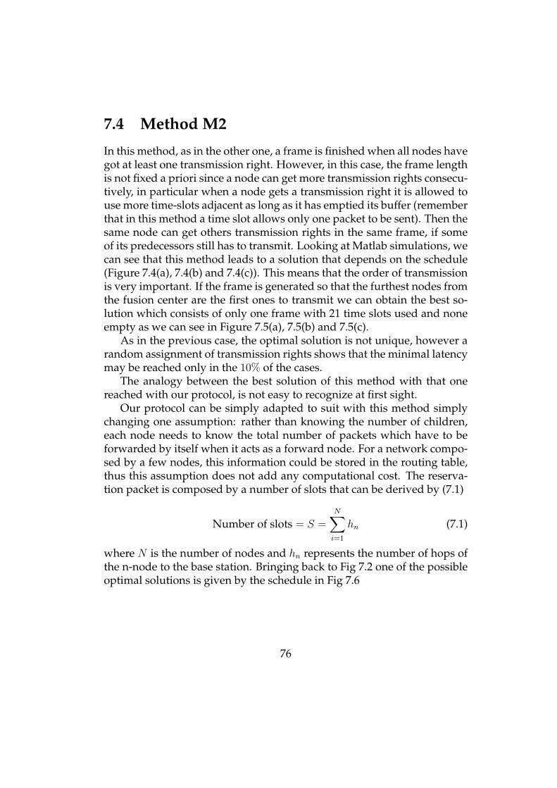
7.4 Method M2

In this method, as in the other one, a frame is finished when all nodes havegot at least one transmission right. However, in this case, the frame lengthis not fixed a priori since a node can get more transmission rights consecu-tively, in particular when a node gets a transmission right it is allowed touse more time-slots adjacent as long as it has emptied its buffer (rememberthat in this method a time slot allows only one packet to be sent). Then thesame node can get others transmission rights in the same frame, if someof its predecessors still has to transmit. Looking at Matlab simulations, wecan see that this method leads to a solution that depends on the schedule(Figure 7.4(a), 7.4(b) and 7.4(c)). This means that the order of transmissionis very important. If the frame is generated so that the furthest nodes fromthe fusion center are the first ones to transmit we can obtain the best so-lution which consists of only one frame with 21 time slots used and noneempty as we can see in Figure 7.5(a), 7.5(b) and 7.5(c).

As in the previous case, the optimal solution is not unique, however arandom assignment of transmission rights shows that the minimal latencymay be reached only in the 10% of the cases.

The analogy between the best solution of this method with that onereached with our protocol, is not easy to recognize at first sight.

Our protocol can be simply adapted to suit with this method simplychanging one assumption: rather than knowing the number of children,each node needs to know the total number of packets which have to beforwarded by itself when it acts as a forward node. For a network compo-sed by a few nodes, this information could be stored in the routing table,thus this assumption does not add any computational cost. The reserva-tion packet is composed by a number of slots that can be derived by (7.1)

Number of slots = S =N∑

i=1

hn (7.1)

where N is the number of nodes and hn represents the number of hops ofthe n-node to the base station. Bringing back to Fig 7.2 one of the possibleoptimal solutions is given by the schedule in Fig 7.6

76

7.5 Conclusions results

We have explained in detail two methods to evaluate the latency in thecase of a simple network consisting of 11 nodes and a fusion center, whichis able to generate a schedule randomly selecting among all the users. Interms of latency (remember that we refer to the number of mini-slot tocalculate the latency), method M2 is clearly the better one: in our simplenetwork the latency is 21 mini-slot compared to 121 mini-slots of methodM1. Our protocol is well-suited for both methods and gives a strong im-provement over a casual schedule, Fig. 7.7.

77

0 1 2 3 4 5 6 7 8 9 100

100

200

300

400

500

600

700

800

Number of frames per schedule

Fre

quen

cy

(a) Latency in terms of frame per sche-dule. Best method M1 has 1 frame

0 50 100 150 200 250 300 350 4000

100

200

300

400

500

600

700

800

Dimension of the schedule in mini−slots

Fre

quen

cy

(b) Dimension of the schedule in mini-slots. Optimal dimension obtained bymethod M1 is 121 mini-slots

0 50 100 150 200 250 300 350 4000

100

200

300

400

500

600

700

800

Empty mini−slots

Fre

quen

cy

(c) Number of empty mini-slots perschedule. The optimal solution consistsin 100 empty mini-slots

Figure 7.3: Latency analysis in Method M1.

78

0 1 2 3 4 5 6 7 8 9 100

100

200

300

400

500

600

Number of frames per schedule

Fre

quen

cy

(a) Latency in terms of frame per sche-dule.

0 10 20 30 40 50 60 70 80 90 1000

50

100

150

200

250

Dimension of the schedule

Fre

quen

cy

(b) Dimension of the schedule.

0 10 20 30 40 50 60 70 80 90 1000

50

100

150

200

250

Empty slots

Fre

quen

cy

(c) Number of empty-slots per schedule.

Figure 7.4: Latency analysis in Method M2.

79

0 1 2 3 4 5 6 7 8 9 100

0.1

0.2

0.3

0.4

0.5

0.6

0.7

0.8

0.9

1

Number of frames per schedule

Fre

quen

cy

(a) Latency in terms of frame per sche-dule.

0 5 10 15 20 25 30 35 40 45 500

0.1

0.2

0.3

0.4

0.5

0.6

0.7

0.8

0.9

1

Dimension of the schedule

Fre

quen

cy

(b) Dimension of the schedule.

0 5 10 15 20 25 30 35 40 45 500

0.1

0.2

0.3

0.4

0.5

0.6

0.7

0.8

0.9

1

Empty slots

Fre

quen

cy

(c) Number of empty-slots per schedule.

Figure 7.5: Latency analysis in Method M2 in the optimal case.

107 8 6 6 6 45 11 9 99 1 3 2 224444

Figure 7.6: Possible schedule for the optimal solution

80

0 10 20 30 40 50 60 70 80 90 1000

50

100

150

200

250

Dimension of the schedule

Fre

quen

cy

(a) Dimension of the schedule in M2.

0 10 20 30 40 50 60 70 80 90 1000

50

100

150

200

250

Empty slots

Fre

quen

cy

(b) Number of empty-slots per schedulein M2.

0 50 100 150 200 250 300 350 4000

100

200

300

400

500

600

700

800

Dimension of the schedule in mini−slots

Fre

quen

cy

(c) Dimension of the schedule in M1.

0 50 100 150 200 250 300 350 4000

100

200

300

400

500

600

700

800

Empty mini−slots

Fre

quen

cy

(d) Number of empty-slots per schedulein M1.

Figure 7.7: Comparison between Method M2 and M1.

81

Chapter 8

Conclusions & future work

8.1 Conclusions

Wireless sensor networks can be used for a wide range of applicationareas(e.g., military, home, environment), each of which poses its own par-ticular technical issues. One key problem that arises in many applications,is how to organize the computation and communication in a sensor net-work to enable accurate estimation of the state of a dynamic system.

As starting point in this thesis, we demonstrate that the performancesof the optimal estimator are influenced by packet loss and delays. Thus,when we want to use a sensor network platform to collect data and for-ward measurements to a data collector, it is critical to understand the lossperformance of the current platform and, possibly, to design MAC sche-mes that eliminate losses and minimize latency.

The main effort of this thesis has been to improve the performance ofthe Telos Tmote sky in terms of data rate. As the sensors are not intendedfor high rate applications the default throughput in terms of packet persecond was very poor. Investigating on the hardware and software of themotes we have been able to obtain a throughput suitable for high rateapplications.

The natural effect of increasing the number of packets per second re-sults in an huge amount of traffic in the network. Telos motes use a CSMA/CAprotocol to access the channel, i.e. there is not synchronization a priori,this results into a great collision probability. To solve the problem of datadelay and to avoid the collisions that lead to packet losses, we propose

82

an overlay TDMA over CSMA. Using a distributed algorithm, as it is ouroverlay TDMA, we can schedule the nodes to have the minimal latencyand to avoid collisions. To show the benefits of our protocol we simulatethe behavior of a general network in which nodes are randomly scheduledby the fusion center. Our protocol permits to obtain, in a distributed way,the optimal solution of such a network resulting in a strong improvementover a casual schedule.

8.2 Future work

A good point for a future work could be a more detailed understandingof the performance bottlenecks. It could be useful to understand if thebottlenecks for the limited rate depend on the saturation of the CPU, or onthe collision of packets or on some external interference.

As we did a theoretical investigation on how delays influence the op-timal estimator performance, we would like to write an application thatstamps a timer into the payload of the node’s packet, so that when thispacket is received by the base station, we can check its latency.

Finally another good point for a future work could be to implementour MAC protocol on the sensors and see the practical performance.

83

Bibliography

[1] Chipcon web site. In http://www.chipcon.com.

[2] Citris annual report 2004-2004. Inhttp://citris.ucdavis.edu/annualreport.pdf.

[3] Cygwin web site. In http://www.cygwin.com.

[4] Moteiv web page. In http://www.moteiv.com.

[5] Tinyos tutorial. In http//www.tinyos.net/tinyos-1.x/doc/tutorial/, Sep-tember 2003.

[6] Chipcon data sheet. In http://www.chipcon.com/files/CC2420 Data Sheet 1 2.pdf,September 2004.

[7] Intel research group. In Instrumenting the world, 2004.

[8] Tinyos community forum. In http//www.tinyos.net, 2004.

[9] I. Akyildiz, W. Su, Y. Sankarasubramaniam, and E. Cayirci. A surveyon sensor networks. In IEEE Communications Magazine, volume 40,pages 102–114, August 2002.

[10] A. Bonivento, C. Fischione, A. Sangiovanni-Vincentelli, F. Graziosi,and F. Santucci. Seran: A semi random protocol solution for cluste-red wireless sensor networks. In International Workshop on LocalizedCommunication and Topology Protocols for Ad hoc Networks, November2005. To appear.

84

[11] B. Bougard, F. Catthoor, D. Daly, A. Chandrakasan, and W. Dehaene.Energy efficiency of the IEEE 802.15.4 standard in dense wireless mi-crosensor networks: modeling and improvement perspectives. In De-sign, Automation and Test in Europe, 2005. Proceedings, volume 1, pages196–201, 2005.

[12] A. Boulis, S. Ganeriwal, and M. Srivastava. Aggregation in sensornetworks: an energy-accuracy trade-off. In IEEE First InternationalWorkshop on Sensor Network Protocols and Applications., pages 128–138,May 2003.

[13] A. Cerpa, J. Elson, M. Hamilton, and J. Zhao. Habitat monitoring:application driven for wireless communications technology. In ACMSIGCOMM’2000, April 2001.

[14] L. P. Clarea, G. J. Pottie, and J. R. Agre. Self-organizing distributedsensor networks.

[15] M. Corporation. Tmote sky quick start guide. Inhttp://www.moteiv.com/products/docs/telos-revb-quickstart.pdf, 2004.

[16] D. Gay, D. Culler, P. Levis, and E. Brewer. nesc language referencemanual. May 2003.

[17] J. Gutierrez, M. Naeve, E. Callaway, M. Bourgeois, V. Mitter, andB. Heile. IEEE 802.15.4: a developing standard for low-power low-cost wireless personal area networks. In IEEE Network, volume 15,pages 12–19, Sept.-Oct.

[18] X. Jiang, J. Polastre, and D. Culler. Perpetual environmentally powe-red sensor networks. In Fourth International Symposium on InformationProcessing in Sensor Networks, 2005. IPSN 2005, pages 463–468, April2005.

[19] V. A. K. Sohrabi, J. Gao and G. J. Pottie. Protocols for self-organizationof a wireless sensor network. In Personal Communications, IEEE [seealso IEEE Wireless Communications], volume 7, pages 16 – 27, October2000.

[20] A. Krasnopeev, J.-J. Xiao, and Z.-Q. Luo. Minimum energy decentra-lized estimation in sensor network with correlated sensor noise. In

85

Proceedings of the IEEE International Conference on Acoustics, Speech, andSignal Processing, 2005 ICASSP’05, volume 3, pages 673–676, March2005.

[21] L. Krishnamachari, D. Estrin, and S. Wicker. The impact of data ag-gregation in wireless sensor networks. In 22nd International Conferenceon Distributed Computing Systems Workshops, 2002, pages 574–578, July2002.

[22] L. Krishnamachari, D. Estrin, and S. Wicker. Modelling data-centricrouting in wireless sensor networks. In IEEE INFCOM, 2002, 2002.

[23] R. Krishnan and D. Starobinski. Message-efficient self-organization ofwireless sensor networks. In IEEE Wireless Communications and Net-working, 2003. WCNC 2003., volume 3, pages 1603 – 1608, 16-20 March2003.

[24] G. Lu, B. Krishnamachari, and C. Raghavendra. Performance eva-luation of the IEEE 802.15.4 mac for low-rate low-power wireless net-works. In 18th International Parallel and Distributed Processing Sympo-sium, 2004. Proceedings., page 224, April 2004.

[25] A. Mainwaring, J. Polastre, R. Szewczyk, D. Culler, and J. Anderson.Wireless sensor networks for habitat monitoring. In WSNA’02, Sep-tember 2002.

[26] J. Misic and V. Misic. Duty cycle management in sensor networksbased on 802.15.4 beacon anabled MAC. In Ad hoc & sensor wirelessnetworks, volume 1, pages 207–233, March 2005.

[27] I. C. Molero. Telos and aegis quick start guide. April 2005.

[28] M. Neugebauer, J. Plonnigs, and K. Kabitzsch. A new beacon orderadaptation algorithm for IEEE 802.15.4 networks. In Proceeedings ofthe Second European Workshop on Wireless Sensor Networks, 2005., pages302 – 311, 31 Jan.-2 Feb 2005.

[29] N. Noury, T. Herv, V. Rialle, G. Virone, E. Mercier, G. Morey, A. Moro,and T. Porcheron. Monitoring behavior in home using a smart fallsensor and position sensors. In 1st Annual International, Conference

86

On Microtechnologies in Medicine and Biology, pages 607–610, October2000.

[30] I. of Electrical and E. Engineers. IEEE std 802.15.4. Thecnical report,IEEE, May 2003.

[31] J. Polastre, R. Szewczyk, and D. Culler. Telos: Enabling Ultra-Low Po-wer Wireless Research. 26-27 April 2005.

[32] M. Rabbat and R. Nowak. Distributed optimization in sensor net-works. In Third International Symposium on Information Processing inSensor Networks 2004, pages 20–27, April 2004.

[33] SENSIRION. STH1x/STH7x humidity & temperature sensors. Inhttp://www.sensirion.com/images/getFile?id=25, July 2004.

[34] J. Thorn. Deciphering tinyos serial packets. In Octave Tech Brief #5-01,March 2005.

[35] J.-J. Xiao, S. Cui, and A. J. Goldsmith. Optimal power schedulingof universal decentralized estimation in sensor networks. November2004.

[36] L. Xiao, S. Boyd, and S. Lall. A scheme for robust distributed sensorfusion based on average consensus.

87