package 'rms
TRANSCRIPT

Package ‘rms’January 7, 2018
Version 5.1-2
Date 2018-01-06
Title Regression Modeling Strategies
Author Frank E Harrell Jr <[email protected]>
Maintainer Frank E Harrell Jr <[email protected]>
Depends Hmisc (>= 4.1-0), survival (>= 2.40-1), lattice, ggplot2 (>=2.2), SparseM
Imports methods, quantreg, rpart, nlme (>= 3.1-123), polspline,multcomp, htmlTable (>= 1.11.0), htmltools
Suggests boot, tcltk, plotly (>= 4.5.6)
Description Regression modeling, testing, estimation, validation,graphics, prediction, and typesetting by storing enhanced model designattributes in the fit. 'rms' is a collection of functions thatassist with and streamline modeling. It also contains functions forbinary and ordinal logistic regression models, ordinal models forcontinuous Y with a variety of distribution families, and the Buckley-Jamesmultiple regression model for right-censored responses, and implementspenalized maximum likelihood estimation for logistic and ordinarylinear models. 'rms' works with almost any regression model, but itwas especially written to work with binary or ordinal regressionmodels, Cox regression, accelerated failure time models,ordinary linear models,the Buckley-James model, generalized leastsquares for serially or spatially correlated observations, generalizedlinear models, and quantile regression.
License GPL (>= 2)
URL http://biostat.mc.vanderbilt.edu/rms
LazyLoad yes
NeedsCompilation yes
Repository CRAN
Date/Publication 2018-01-07 22:27:43 UTC
1

2 R topics documented:
R topics documented:anova.rms . . . . . . . . . . . . . . . . . . . . . . . . . . . . . . . . . . . . . . . . . . 3bj . . . . . . . . . . . . . . . . . . . . . . . . . . . . . . . . . . . . . . . . . . . . . . 9bootBCa . . . . . . . . . . . . . . . . . . . . . . . . . . . . . . . . . . . . . . . . . . . 13bootcov . . . . . . . . . . . . . . . . . . . . . . . . . . . . . . . . . . . . . . . . . . . 15bplot . . . . . . . . . . . . . . . . . . . . . . . . . . . . . . . . . . . . . . . . . . . . . 23calibrate . . . . . . . . . . . . . . . . . . . . . . . . . . . . . . . . . . . . . . . . . . . 26contrast.rms . . . . . . . . . . . . . . . . . . . . . . . . . . . . . . . . . . . . . . . . . 30cph . . . . . . . . . . . . . . . . . . . . . . . . . . . . . . . . . . . . . . . . . . . . . . 36cr.setup . . . . . . . . . . . . . . . . . . . . . . . . . . . . . . . . . . . . . . . . . . . 43datadist . . . . . . . . . . . . . . . . . . . . . . . . . . . . . . . . . . . . . . . . . . . 46ExProb . . . . . . . . . . . . . . . . . . . . . . . . . . . . . . . . . . . . . . . . . . . 48fastbw . . . . . . . . . . . . . . . . . . . . . . . . . . . . . . . . . . . . . . . . . . . . 50Function . . . . . . . . . . . . . . . . . . . . . . . . . . . . . . . . . . . . . . . . . . . 52gendata . . . . . . . . . . . . . . . . . . . . . . . . . . . . . . . . . . . . . . . . . . . 54ggplot.Predict . . . . . . . . . . . . . . . . . . . . . . . . . . . . . . . . . . . . . . . . 56gIndex . . . . . . . . . . . . . . . . . . . . . . . . . . . . . . . . . . . . . . . . . . . . 64Glm . . . . . . . . . . . . . . . . . . . . . . . . . . . . . . . . . . . . . . . . . . . . . 68Gls . . . . . . . . . . . . . . . . . . . . . . . . . . . . . . . . . . . . . . . . . . . . . . 69groupkm . . . . . . . . . . . . . . . . . . . . . . . . . . . . . . . . . . . . . . . . . . . 72hazard.ratio.plot . . . . . . . . . . . . . . . . . . . . . . . . . . . . . . . . . . . . . . . 74ie.setup . . . . . . . . . . . . . . . . . . . . . . . . . . . . . . . . . . . . . . . . . . . 75latex.cph . . . . . . . . . . . . . . . . . . . . . . . . . . . . . . . . . . . . . . . . . . . 77latexrms . . . . . . . . . . . . . . . . . . . . . . . . . . . . . . . . . . . . . . . . . . . 79lrm . . . . . . . . . . . . . . . . . . . . . . . . . . . . . . . . . . . . . . . . . . . . . . 81lrm.fit . . . . . . . . . . . . . . . . . . . . . . . . . . . . . . . . . . . . . . . . . . . . 89matinv . . . . . . . . . . . . . . . . . . . . . . . . . . . . . . . . . . . . . . . . . . . . 91nomogram . . . . . . . . . . . . . . . . . . . . . . . . . . . . . . . . . . . . . . . . . . 93npsurv . . . . . . . . . . . . . . . . . . . . . . . . . . . . . . . . . . . . . . . . . . . . 100ols . . . . . . . . . . . . . . . . . . . . . . . . . . . . . . . . . . . . . . . . . . . . . . 101orm . . . . . . . . . . . . . . . . . . . . . . . . . . . . . . . . . . . . . . . . . . . . . 105orm.fit . . . . . . . . . . . . . . . . . . . . . . . . . . . . . . . . . . . . . . . . . . . . 111pentrace . . . . . . . . . . . . . . . . . . . . . . . . . . . . . . . . . . . . . . . . . . . 114plot.Predict . . . . . . . . . . . . . . . . . . . . . . . . . . . . . . . . . . . . . . . . . 117plot.xmean.ordinaly . . . . . . . . . . . . . . . . . . . . . . . . . . . . . . . . . . . . . 125plotp.Predict . . . . . . . . . . . . . . . . . . . . . . . . . . . . . . . . . . . . . . . . . 127pphsm . . . . . . . . . . . . . . . . . . . . . . . . . . . . . . . . . . . . . . . . . . . . 130predab.resample . . . . . . . . . . . . . . . . . . . . . . . . . . . . . . . . . . . . . . . 131Predict . . . . . . . . . . . . . . . . . . . . . . . . . . . . . . . . . . . . . . . . . . . . 135predict.lrm . . . . . . . . . . . . . . . . . . . . . . . . . . . . . . . . . . . . . . . . . . 140predictrms . . . . . . . . . . . . . . . . . . . . . . . . . . . . . . . . . . . . . . . . . . 142print.cph . . . . . . . . . . . . . . . . . . . . . . . . . . . . . . . . . . . . . . . . . . . 149print.ols . . . . . . . . . . . . . . . . . . . . . . . . . . . . . . . . . . . . . . . . . . . 150psm . . . . . . . . . . . . . . . . . . . . . . . . . . . . . . . . . . . . . . . . . . . . . 151residuals.cph . . . . . . . . . . . . . . . . . . . . . . . . . . . . . . . . . . . . . . . . 155residuals.lrm . . . . . . . . . . . . . . . . . . . . . . . . . . . . . . . . . . . . . . . . . 157residuals.ols . . . . . . . . . . . . . . . . . . . . . . . . . . . . . . . . . . . . . . . . . 163
anova.rms 3
rms . . . . . . . . . . . . . . . . . . . . . . . . . . . . . . . . . . . . . . . . . . . . . 164rms.trans . . . . . . . . . . . . . . . . . . . . . . . . . . . . . . . . . . . . . . . . . . . 167rmsMisc . . . . . . . . . . . . . . . . . . . . . . . . . . . . . . . . . . . . . . . . . . . 169rmsOverview . . . . . . . . . . . . . . . . . . . . . . . . . . . . . . . . . . . . . . . . 175robcov . . . . . . . . . . . . . . . . . . . . . . . . . . . . . . . . . . . . . . . . . . . . 187Rq . . . . . . . . . . . . . . . . . . . . . . . . . . . . . . . . . . . . . . . . . . . . . . 189sensuc . . . . . . . . . . . . . . . . . . . . . . . . . . . . . . . . . . . . . . . . . . . . 192setPb . . . . . . . . . . . . . . . . . . . . . . . . . . . . . . . . . . . . . . . . . . . . . 195specs.rms . . . . . . . . . . . . . . . . . . . . . . . . . . . . . . . . . . . . . . . . . . 197summary.rms . . . . . . . . . . . . . . . . . . . . . . . . . . . . . . . . . . . . . . . . 198survest.cph . . . . . . . . . . . . . . . . . . . . . . . . . . . . . . . . . . . . . . . . . 202survest.psm . . . . . . . . . . . . . . . . . . . . . . . . . . . . . . . . . . . . . . . . . 205survfit.cph . . . . . . . . . . . . . . . . . . . . . . . . . . . . . . . . . . . . . . . . . . 207survplot . . . . . . . . . . . . . . . . . . . . . . . . . . . . . . . . . . . . . . . . . . . 208val.prob . . . . . . . . . . . . . . . . . . . . . . . . . . . . . . . . . . . . . . . . . . . 215val.surv . . . . . . . . . . . . . . . . . . . . . . . . . . . . . . . . . . . . . . . . . . . 220validate . . . . . . . . . . . . . . . . . . . . . . . . . . . . . . . . . . . . . . . . . . . 224validate.cph . . . . . . . . . . . . . . . . . . . . . . . . . . . . . . . . . . . . . . . . . 226validate.lrm . . . . . . . . . . . . . . . . . . . . . . . . . . . . . . . . . . . . . . . . . 229validate.ols . . . . . . . . . . . . . . . . . . . . . . . . . . . . . . . . . . . . . . . . . 232validate.rpart . . . . . . . . . . . . . . . . . . . . . . . . . . . . . . . . . . . . . . . . 233validate.Rq . . . . . . . . . . . . . . . . . . . . . . . . . . . . . . . . . . . . . . . . . 235vif . . . . . . . . . . . . . . . . . . . . . . . . . . . . . . . . . . . . . . . . . . . . . . 237which.influence . . . . . . . . . . . . . . . . . . . . . . . . . . . . . . . . . . . . . . . 238
Index 240
anova.rms Analysis of Variance (Wald and F Statistics)
Description
The anova function automatically tests most meaningful hypotheses in a design. For example,suppose that age and cholesterol are predictors, and that a general interaction is modeled using arestricted spline surface. anova prints Wald statistics (F statistics for an ols fit) for testing linearityof age, linearity of cholesterol, age effect (age + age by cholesterol interaction), cholesterol effect(cholesterol + age by cholesterol interaction), linearity of the age by cholesterol interaction (i.e.,adequacy of the simple age * cholesterol 1 d.f. product), linearity of the interaction in age alone,and linearity of the interaction in cholesterol alone. Joint tests of all interaction terms in the modeland all nonlinear terms in the model are also performed. For any multiple d.f. effects for continuousvariables that were not modeled through rcs, pol, lsp, etc., tests of linearity will be omitted.This applies to matrix predictors produced by e.g. poly or ns. print.anova.rms is the printingmethod. plot.anova.rms draws dot charts depicting the importance of variables in the model,as measured by Wald χ2, χ2 minus d.f., AIC, P -values, partial R2, R2 for the whole model afterdeleting the effects in question, or proportion of overall model R2 that is due to each predictor.latex.anova.rms is the latex method. It substitutes Greek/math symbols in column headings,uses boldface for TOTAL lines, and constructs a caption. Then it passes the result to latex.defaultfor conversion to LaTeX.
4 anova.rms
The print method calls latex or html methods depending on options(prType=), and output isto the console. For latex a table environment is not used and an ordinary tabular is produced.
html.anova.rms just calls latex.anova.rms.
Usage
## S3 method for class 'rms'anova(object, ..., main.effect=FALSE, tol=1e-9,
test=c('F','Chisq'), india=TRUE, indnl=TRUE, ss=TRUE,vnames=c('names','labels'))
## S3 method for class 'anova.rms'print(x,
which=c('none','subscripts','names','dots'),table.env=FALSE, ...)
## S3 method for class 'anova.rms'plot(x,
what=c("chisqminusdf","chisq","aic","P","partial R2","remaining R2","proportion R2", "proportion chisq"),
xlab=NULL, pch=16,rm.totals=TRUE, rm.ia=FALSE, rm.other=NULL, newnames,sort=c("descending","ascending","none"), margin=c('chisq','P'),pl=TRUE, trans=NULL, ntrans=40, height=NULL, width=NULL, ...)
## S3 method for class 'anova.rms'latex(object, title, dec.chisq=2,
dec.F=2, dec.ss=NA, dec.ms=NA, dec.P=4, table.env=TRUE,caption=NULL, ...)
## S3 method for class 'anova.rms'html(object, ...)
Arguments
object a rms fit object. object must allow vcov to return the variance-covariance ma-trix. For latex is the result of anova.
... If omitted, all variables are tested, yielding tests for individual factors and forpooled effects. Specify a subset of the variables to obtain tests for only thosefactors, with a pooled Wald tests for the combined effects of all factors listed.Names may be abbreviated. For example, specify anova(fit,age,cholesterol)to get a Wald statistic for testing the joint importance of age, cholesterol, and anyfactor interacting with them.Can be optional graphical parameters to send to dotchart2, or other parametersto send to latex.default. Ignored for print.For html.anova.rms the arguments are passed to latex.anova.rms.
main.effect Set to TRUE to print the (usually meaningless) main effect tests even when thefactor is involved in an interaction. The default is FALSE, to print only the effect

anova.rms 5
of the main effect combined with all interactions involving that factor.
tol singularity criterion for use in matrix inversion
test For an ols fit, set test="Chisq" to use Wald χ2 tests rather than F-tests.
india set to FALSE to exclude individual tests of interaction from the table
indnl set to FALSE to exclude individual tests of nonlinearity from the table
ss For an ols fit, set ss=FALSE to suppress printing partial sums of squares, meansquares, and the Error SS and MS.
vnames set to 'labels' to use variable labels rather than variable names in the output
x for print,plot,text is the result of anova.
which If which is not "none" (the default), print.anova.rms will add to the right-most column of the output the list of parameters being tested by the hypothesisbeing tested in the current row. Specifying which="subscripts" causes thesubscripts of the regression coefficients being tested to be printed (with a sub-script of one for the first non-intercept term). which="names" prints the namesof the terms being tested, and which="dots" prints dots for terms being testedand blanks for those just being adjusted for.
what what type of statistic to plot. The default is the Wald χ2 statistic for each factor(adding in the effect of higher-ordered factors containing that factor) minus itsdegrees of freedom. The R2 choices for what only apply to ols models.
xlab x-axis label, default is constructed according to what. plotmath symbols areused for R, by default.
pch character for plotting dots in dot charts. Default is 16 (solid dot).
rm.totals set to FALSE to keep total χ2s (overall, nonlinear, interaction totals) in the chart.
rm.ia set to TRUE to omit any effect that has "*" in its name
rm.other a list of other predictor names to omit from the chart
newnames a list of substitute predictor names to use, after omitting any.
sort default is to sort bars in descending order of the summary statistic
margin set to a vector of character strings to write text for selected statistics in theright margin of the dot chart. The character strings can be any combination of"chisq", "d.f.", "P", "partial R2", "proportion R2", and "proportion chisq".Default is to not draw any statistics in the margin. When plotly is in effect,margin values are instead displayed as hover text.
pl set to FALSE to suppress plotting. This is useful when you only wish to analyzethe vector of statistics returned.
trans set to a function to apply that transformation to the statistics being plotted, andto truncate negative values at zero. A good choice is trans=sqrt.
ntrans n argument to pretty, specifying the number of values for which to place tickmarks. This should be larger than usual because of nonlinear scaling, to providea sufficient number of tick marks on the left (stretched) part of the chi-squarescale.
height,width height and width of plotly plots drawn using dotchartp, in pixels. Ignored forordinary plots. Defaults to minimum of 400 and 100 + 25 times the number oftest statistics displayed.

6 anova.rms
title title to pass to latex, default is name of fit object passed to anova prefixed with"anova.". For Windows, the default is "ano" followed by the first 5 letters ofthe name of the fit object.
dec.chisq number of places to the right of the decimal place for typesetting χ2 values(default is 2). Use zero for integer, NA for floating point.
dec.F digits to the right for F statistics (default is 2)
dec.ss digits to the right for sums of squares (default is NA, indicating floating point)
dec.ms digits to the right for mean squares (default is NA)
dec.P digits to the right for P -values
table.env see latex
caption caption for table if table.env is TRUE. Default is constructed from the responsevariable.
Details
If the statistics being plotted with plot.anova.rms are few in number and one of them is negativeor zero, plot.anova.rms will quit because of an error in dotchart2.
Value
anova.rms returns a matrix of class anova.rms containing factors as rows and χ2, d.f., and P -values as columns (or d.f., partial SS,MS,F, P ). An attribute vinfo provides list of variablesinvolved in each row and the type of test done. plot.anova.rms invisibly returns the vector ofquantities plotted. This vector has a names attribute describing the terms for which the statistics inthe vector are calculated.
Side Effects
print prints, latex creates a file with a name of the form "title.tex" (see the title argumentabove).
Author(s)
Frank HarrellDepartment of Biostatistics, Vanderbilt [email protected]
See Also
rms, rmsMisc, lrtest, rms.trans, summary.rms, plot.Predict, ggplot.Predict, solvet, locator,dotchart2, latex, xYplot, anova.lm, contrast.rms, pantext
Examples
n <- 1000 # define sample sizeset.seed(17) # so can reproduce the resultstreat <- factor(sample(c('a','b','c'), n,TRUE))num.diseases <- sample(0:4, n,TRUE)
anova.rms 7
age <- rnorm(n, 50, 10)cholesterol <- rnorm(n, 200, 25)weight <- rnorm(n, 150, 20)sex <- factor(sample(c('female','male'), n,TRUE))label(age) <- 'Age' # label is in Hmisclabel(num.diseases) <- 'Number of Comorbid Diseases'label(cholesterol) <- 'Total Cholesterol'label(weight) <- 'Weight, lbs.'label(sex) <- 'Sex'units(cholesterol) <- 'mg/dl' # uses units.default in Hmisc
# Specify population model for log odds that Y=1L <- .1*(num.diseases-2) + .045*(age-50) +
(log(cholesterol - 10)-5.2)*(-2*(treat=='a') +3.5*(treat=='b')+2*(treat=='c'))
# Simulate binary y to have Prob(y=1) = 1/[1+exp(-L)]y <- ifelse(runif(n) < plogis(L), 1, 0)
fit <- lrm(y ~ treat + scored(num.diseases) + rcs(age) +log(cholesterol+10) + treat:log(cholesterol+10))
a <- anova(fit) # Test all factorsb <- anova(fit, treat, cholesterol) # Test these 2 by themselves
# to get their pooled effectsab# Add a new line to the plot with combined effectss <- rbind(a, 'treat+cholesterol'=b['TOTAL',])class(s) <- 'anova.rms'plot(s, margin=c('chisq', 'proportion chisq'))
g <- lrm(y ~ treat*rcs(age))dd <- datadist(treat, num.diseases, age, cholesterol)options(datadist='dd')p <- Predict(g, age, treat="b")s <- anova(g)# Usually omit fontfamily to default to 'Courier'# It's specified here to make R pass its package-building checksplot(p, addpanel=pantext(s, 28, 1.9, fontfamily='Helvetica'))
plot(s, margin=c('chisq', 'proportion chisq'))# new plot - dot chart of chisq-d.f. with 2 other stats in right margin# latex(s) # nice printout - creates anova.g.texoptions(datadist=NULL)
# Simulate data with from a given model, and display exactly which# hypotheses are being tested
set.seed(123)age <- rnorm(500, 50, 15)
8 anova.rms
treat <- factor(sample(c('a','b','c'), 500, TRUE))bp <- rnorm(500, 120, 10)y <- ifelse(treat=='a', (age-50)*.05, abs(age-50)*.08) + 3*(treat=='c') +
pmax(bp, 100)*.09 + rnorm(500)f <- ols(y ~ treat*lsp(age,50) + rcs(bp,4))print(names(coef(f)), quote=FALSE)specs(f)anova(f)an <- anova(f)options(digits=3)print(an, 'subscripts')print(an, 'dots')
an <- anova(f, test='Chisq', ss=FALSE)plot(0:1) # make some plottab <- pantext(an, 1.2, .6, lattice=FALSE, fontfamily='Helvetica')# create function to write table; usually omit fontfamilytab() # execute it; could do tab(cex=.65)plot(an) # new plot - dot chart of chisq-d.f.# Specify plot(an, trans=sqrt) to use a square root scale for this plot# latex(an) # nice printout - creates anova.f.tex
## Example to save partial R^2 for all predictors, along with overall## R^2, from two separate fits, and to combine them with a lattice plot
require(lattice)set.seed(1)n <- 100x1 <- runif(n)x2 <- runif(n)y <- (x1-.5)^2 + x2 + runif(n)group <- c(rep('a', n/2), rep('b', n/2))A <- NULLfor(g in c('a','b')) {
f <- ols(y ~ pol(x1,2) + pol(x2,2) + pol(x1,2) %ia% pol(x2,2),subset=group==g)
a <- plot(anova(f),what='partial R2', pl=FALSE, rm.totals=FALSE, sort='none')
a <- a[-grep('NONLINEAR', names(a))]d <- data.frame(group=g, Variable=factor(names(a), names(a)),
partialR2=unname(a))A <- rbind(A, d)
}dotplot(Variable ~ partialR2 | group, data=A,
xlab=ex <- expression(partial~R^2))dotplot(group ~ partialR2 | Variable, data=A, xlab=ex)dotplot(Variable ~ partialR2, groups=group, data=A, xlab=ex,
auto.key=list(corner=c(.5,.5)))
# Suppose that a researcher wants to make a big deal about a variable
bj 9
# because it has the highest adjusted chi-square. We use the# bootstrap to derive 0.95 confidence intervals for the ranks of all# the effects in the model. We use the plot method for anova, with# pl=FALSE to suppress actual plotting of chi-square - d.f. for each# bootstrap repetition.# It is important to tell plot.anova.rms not to sort the results, or# every bootstrap replication would have ranks of 1,2,3,... for the stats.
n <- 300set.seed(1)d <- data.frame(x1=runif(n), x2=runif(n), x3=runif(n),
x4=runif(n), x5=runif(n), x6=runif(n), x7=runif(n),x8=runif(n), x9=runif(n), x10=runif(n), x11=runif(n),x12=runif(n))
d$y <- with(d, 1*x1 + 2*x2 + 3*x3 + 4*x4 + 5*x5 + 6*x6 +7*x7 + 8*x8 + 9*x9 + 10*x10 + 11*x11 +12*x12 + 9*rnorm(n))
f <- ols(y ~ x1+x2+x3+x4+x5+x6+x7+x8+x9+x10+x11+x12, data=d)B <- 20 # actually use B=1000ranks <- matrix(NA, nrow=B, ncol=12)rankvars <- function(fit)
rank(plot(anova(fit), sort='none', pl=FALSE))Rank <- rankvars(f)for(i in 1:B) {
j <- sample(1:n, n, TRUE)bootfit <- update(f, data=d, subset=j)ranks[i,] <- rankvars(bootfit)}
lim <- t(apply(ranks, 2, quantile, probs=c(.025,.975)))predictor <- factor(names(Rank), names(Rank))Dotplot(predictor ~ Cbind(Rank, lim), pch=3, xlab='Rank')
bj Buckley-James Multiple Regression Model
Description
bj fits the Buckley-James distribution-free least squares multiple regression model to a possiblyright-censored response variable. This model reduces to ordinary least squares if there is no cen-soring. By default, model fitting is done after taking logs of the response variable. bj uses the rmsclass for automatic anova, fastbw, validate, Function, nomogram, summary, plot, bootcov, andother functions. The bootcov function may be worth using with bj fits, as the properties of theBuckley-James covariance matrix estimator are not fully known for strange censoring patterns.
For the print method, format of output is controlled by the user previously running options(prType="lang")where lang is "plain" (the default), "latex", or "html".
The residuals.bj function exists mainly to compute residuals and to censor them (i.e., returnthem as Surv objects) just as the original failure time variable was censored. These residuals are
10 bj
useful for checking to see if the model also satisfies certain distributional assumptions. To get theseresiduals, the fit must have specified y=TRUE.
The bjplot function is a special plotting function for objects created by bj with x=TRUE, y=TRUEin effect. It produces three scatterplots for every covariate in the model: the first plots the originalsituation, where censored data are distingushed from non-censored data by a different plotting sym-bol. In the second plot, called a renovated plot, vertical lines show how censored data were changedby the procedure, and the third is equal to the second, but without vertical lines. Imputed data areagain distinguished from the non-censored by a different symbol.
The validate method for bj validates the Somers’ Dxy rank correlation between predicted andobserved responses, accounting for censoring.
The primary fitting function for bj is bj.fit, which does not allow missing data and expects a fulldesign matrix as input.
Usage
bj(formula=formula(data), data, subset, na.action=na.delete,link="log", control, method='fit', x=FALSE, y=FALSE,time.inc)
## S3 method for class 'bj'print(x, digits=4, long=FALSE, coefs=TRUE,title="Buckley-James Censored Data Regression", ...)
## S3 method for class 'bj'residuals(object, type=c("censored","censored.normalized"),...)
bjplot(fit, which=1:dim(X)[[2]])
## S3 method for class 'bj'validate(fit, method="boot", B=40,
bw=FALSE,rule="aic",type="residual",sls=.05,aics=0,force=NULL, estimates=TRUE, pr=FALSE,
tol=1e-7, rel.tolerance=1e-3, maxiter=15, ...)
bj.fit(x, y, control)
Arguments
formula an S statistical model formula. Interactions up to third order are supported. Theleft hand side must be a Surv object.
data,subset,na.action
the usual statistical model fitting arguments
fit a fit created by bj, required for all functions except bj.
x a design matrix with or without a first column of ones, to pass to bj.fit. Allmodels will have an intercept. For print.bj is a result of bj. For bj, set x=TRUEto include the design matrix in the fit object.
bj 11
y a Surv object to pass to bj.fit as the two-column response variable. Only rightcensoring is allowed, and there need not be any censoring. For bj, set y to TRUEto include the two-column response matrix, with the event/censoring indicatorin the second column. The first column will be transformed according to link,and depending on na.action, rows with missing data in the predictors or theresponse will be deleted.
link set to, for example, "log" (the default) to model the log of the response, or"identity" to model the untransformed response.
control a list containing any or all of the following components: iter.max (maximumnumber of iterations allowed, default is 20), eps (convergence criterion: concer-gence is assumed when the ratio of sum of squared errors from one iteration tothe next is between 1-eps and 1+eps), trace (set to TRUE to monitor iterations),tol (matrix singularity criterion, default is 1e-7), and ’max.cycle’ (in case ofnonconvergence the program looks for a cycle that repeats itself, default is 30).
method set to "model.frame" or "model.matrix" to return one of those objects ratherthan the model fit.
time.inc setting for default time spacing. Default is 30 if time variable has units="Day",1 otherwise, unless maximum follow-up time < 1. Then max time/10 is usedas time.inc. If time.inc is not given and max time/default time.inc is > 25,time.inc is increased.
digits number of significant digits to print if not 4.
long set to TRUE to print the correlation matrix for parameter estimates
coefs specify coefs=FALSE to suppress printing the table of model coefficients, stan-dard errors, etc. Specify coefs=n to print only the first n regression coefficientsin the model.
title a character string title to be passed to prModFit
object the result of bj
type type of residual desired. Default is censored unnormalized residuals, defined aslink(Y) - linear.predictors, where the link function was usually the log function.You can specify type="censored.normalized" to divide the residuals by theestimate of sigma.
which vector of integers or character strings naming elements of the design matrix (thenames of the original predictors if they entered the model linearly) for which tohave bjplot make plots of only the variables listed in which (names or num-bers).
B,bw,rule,sls,aics,force,estimates,pr,tol,rel.tolerance,maxiter
see predab.resample
... ignored for print; passed through to predab.resample for validate
Details
The program implements the algorithm as described in the original article by Buckley & James.Also, we have used the original Buckley & James prescription for computing variance/covarianceestimator. This is based on non-censored observations only and does not have any theoretical jus-tification, but has been shown in simulation studies to behave well. Our experience confirms this
12 bj
view. Convergence is rather slow with this method, so you may want to increase the number ofiterations. Our experience shows that often, in particular with high censoring, 100 iterations is nottoo many. Sometimes the method will not converge, but will instead enter a loop of repeating values(this is due to the discrete nature of Kaplan and Meier estimator and usually happens with smallsample sizes). The program will look for such a loop and return the average betas. It will also issuea warning message and give the size of the cycle (usually less than 6).
Value
bj returns a fit object with similar information to what survreg, psm, cph would store as wellas what rms stores and units and time.inc. residuals.bj returns a Surv object. One of thecomponents of the fit object produced by bj (and bj.fit) is a vector called stats which containsthe following names elements: "Obs", "Events", "d.f.","error d.f.","sigma","g". Heresigma is the estimate of the residual standard deviation. g is the g-index. If the link function is"log", the g-index on the anti-log scale is also returned as gr.
Author(s)
Janez StareDepartment of Biomedical InformaticsLjubljana UniversityLjubljana, Slovenia<[email protected]>
Harald HeinzlDepartment of Medical Computer SciencesVienna UniversityVienna, Austria<[email protected]>
Frank HarrellDepartment of BiostatisticsVanderbilt University<[email protected]>
References
Buckley JJ, James IR. Linear regression with censored data. Biometrika 1979; 66:429–36.
Miller RG, Halpern J. Regression with censored data. Biometrika 1982; 69: 521–31.
James IR, Smith PJ. Consistency results for linear regression with censored data. Ann Statist 1984;12: 590–600.
Lai TL, Ying Z. Large sample theory of a modified Buckley-James estimator for regression analysiswith censored data. Ann Statist 1991; 19: 1370–402.
Hillis SL. Residual plots for the censored data linear regression model. Stat in Med 1995; 14:2023–2036.
Jin Z, Lin DY, Ying Z. On least-squares regression with censored data. Biometrika 2006; 93:147–161.

bootBCa 13
See Also
rms, psm, survreg, cph, Surv, na.delete, na.detail.response, datadist, rcorr.cens, GiniMd,prModFit, dxy.cens
Examples
set.seed(1)ftime <- 10*rexp(200)stroke <- ifelse(ftime > 10, 0, 1)ftime <- pmin(ftime, 10)units(ftime) <- "Month"age <- rnorm(200, 70, 10)hospital <- factor(sample(c('a','b'),200,TRUE))dd <- datadist(age, hospital)options(datadist="dd")
f <- bj(Surv(ftime, stroke) ~ rcs(age,5) + hospital, x=TRUE, y=TRUE)# add link="identity" to use a censored normal regression model instead# of a lognormal oneanova(f)fastbw(f)validate(f, B=15)plot(Predict(f, age, hospital))# needs datadist since no explicit age,hosp.coef(f) # look at regression coefficientscoef(psm(Surv(ftime, stroke) ~ rcs(age,5) + hospital, dist='lognormal'))
# compare with coefficients from likelihood-based# log-normal regression model# use dist='gau' not under R
r <- resid(f, 'censored.normalized')survplot(npsurv(r ~ 1), conf='none')
# plot Kaplan-Meier estimate of# survival function of standardized residuals
survplot(npsurv(r ~ cut2(age, g=2)), conf='none')# may desire both strata to be n(0,1)
options(datadist=NULL)
bootBCa BCa Bootstrap on Existing Bootstrap Replicates
Description
This functions constructs an object resembling one produced by the boot package’s boot func-tion, and runs that package’s boot.ci function to compute BCa and percentile confidence limits.bootBCa can provide separate confidence limits for a vector of statistics when estimate has lengthgreater than 1. In that case, estimates must have the same number of columns as estimate hasvalues.
14 bootBCa
Usage
bootBCa(estimate, estimates, type=c('percentile','bca','basic'),n, seed, conf.int = 0.95)
Arguments
estimate original whole-sample estimate
estimates vector of bootstrap estimates
type type of confidence interval, defaulting to nonparametric percentile
n original number of observations
seed .Random.seem in effect before bootstrap estimates were run
conf.int confidence level
Value
a 2-vector if estimate is of length 1, otherwise a matrix with 2 rows and number of columns equalto the length of estimate
Note
You can use if(!exists('.Random.seed')) runif(1) before running your bootstrap to makesure that .Random.seed will be available to bootBCa.
Author(s)
Frank Harrell
See Also
boot.ci
Examples
## Not run:x1 <- runif(100); x2 <- runif(100); y <- sample(0:1, 100, TRUE)f <- lrm(y ~ x1 + x2, x=TRUE, y=TRUE)seed <- .Random.seedb <- bootcov(f)# Get estimated log odds at x1=.4, x2=.6X <- cbind(c(1,1), x1=c(.4,2), x2=c(.6,3))est <- Xests <- t(XbootBCa(est, ests, n=100, seed=seed)bootBCa(est, ests, type='bca', n=100, seed=seed)bootBCa(est, ests, type='basic', n=100, seed=seed)
## End(Not run)
bootcov 15
bootcov Bootstrap Covariance and Distribution for Regression Coefficients
Description
bootcov computes a bootstrap estimate of the covariance matrix for a set of regression coefficientsfrom ols, lrm, cph, psm, Rq, and any other fit where x=TRUE, y=TRUE was used to store the dataused in making the original regression fit and where an appropriate fitter function is providedhere. The estimates obtained are not conditional on the design matrix, but are instead unconditionalestimates. For small sample sizes, this will make a difference as the unconditional variance esti-mates are larger. This function will also obtain bootstrap estimates corrected for cluster sampling(intra-cluster correlations) when a "working independence" model was used to fit data which werecorrelated within clusters. This is done by substituting cluster sampling with replacement for theusual simple sampling with replacement. bootcov has an option (coef.reps) that causes all ofthe regression coefficient estimates from all of the bootstrap re-samples to be saved, facilitatingcomputation of nonparametric bootstrap confidence limits and plotting of the distributions of thecoefficient estimates (using histograms and kernel smoothing estimates).
The loglik option facilitates the calculation of simultaneous confidence regions from quantitiesof interest that are functions of the regression coefficients, using the method of Tibshirani(1996).With Tibshirani’s method, one computes the objective criterion (-2 log likelihood evaluated at thebootstrap estimate of β but with respect to the original design matrix and response vector) for theoriginal fit as well as for all of the bootstrap fits. The confidence set of the regression coefficients isthe set of all coefficients that are associated with objective function values that are less than or equalto say the 0.95 quantile of the vector of B + 1 objective function values. For the coefficients satis-fying this condition, predicted values are computed at a user-specified design matrix X, and minimaand maxima of these predicted values (over the qualifying bootstrap repetitions) are computed toderive the final simultaneous confidence band.
The bootplot function takes the output of bootcov and either plots a histogram and kernel densityestimate of specified regression coefficients (or linear combinations of them through the use of aspecified design matrix X), or a qqnorm plot of the quantities of interest to check for normality of themaximum likelihood estimates. bootplot draws vertical lines at specified quantiles of the bootstrapdistribution, and returns these quantiles for possible printing by the user. Bootstrap estimates mayoptionally be transformed by a user-specified function fun before plotting.
The confplot function also uses the output of bootcov but to compute and optionally plot non-parametric bootstrap pointwise confidence limits or (by default) Tibshirani (1996) simultaneousconfidence sets. A design matrix must be specified to allow confplot to compute quantities ofinterest such as predicted values across a range of values or differences in predicted values (plots ofeffects of changing one or more predictor variable values).
bootplot and confplot are actually generic functions, with the particular functions bootplot.bootcovand confplot.bootcov automatically invoked for bootcov objects.
A service function called histdensity is also provided (for use with bootplot). It runs hist anddensity on the same plot, using twice the number of classes than the default for hist, and 1.5times the width than the default used by density.
A comprehensive example demonstrates the use of all of the functions.
16 bootcov
Usage
bootcov(fit, cluster, B=200, fitter,coef.reps=TRUE, loglik=FALSE,pr=FALSE, maxit=15, eps=0.0001, group=NULL, stat=NULL)
bootplot(obj, which=1 : ncol(Coef), X,conf.int=c(.9,.95,.99),what=c('density', 'qqnorm', 'box'),fun=function(x) x, labels., ...)
confplot(obj, X, against,method=c('simultaneous','pointwise'),conf.int=0.95, fun=function(x)x,add=FALSE, lty.conf=2, ...)
histdensity(y, xlab, nclass, width, mult.width=1, ...)
Arguments
fit a fit object containing components x and y. For fits from cph, the "strata"attribute of the x component is used to obtain the vector of stratum codes.
obj an object created by bootcov with coef.reps=TRUE.X a design matrix specified to confplot. See predict.rms or contrast.rms.
For bootplot, X is optional.y a vector to pass to histdensity. NAs are ignored.cluster a variable indicating groupings. cluster may be any type of vector (factor,
character, integer). Unique values of cluster indicate possibly correlated group-ings of observations. Note the data used in the fit and stored in fit$x and fit$ymay have had observations containing missing values deleted. It is assumedthat if there were any NAs, an naresid function exists for the class of fit.This function restores NAs so that the rows of the design matrix coincide withcluster.
B number of bootstrap repetitions. Default is 200.fitter the name of a function with arguments (x,y) that will fit bootstrap samples.
Default is taken from the class of fit if it is ols, lrm, cph, psm, Rq.coef.reps set to TRUE if you want to store a matrix of all bootstrap regression coefficient
estimates in the returned component boot.Coef.loglik set to TRUE to store -2 log likelihoods for each bootstrap model, evaluated against
the original x and y data. The default is to do this when coef.reps is specified asTRUE. The use of loglik=TRUE assumes that an oos.loglik method exists forthe type of model being analyzed, to calculate out-of-sample -2 log likelihoods(see rmsMisc). After the B -2 log likelihoods (stored in the element namedboot.loglik in the returned fit object), the B+1 element is the -2 log likelihoodfor the original model fit.

bootcov 17
pr set to TRUE to print the current sample number to monitor progress.
maxit maximum number of iterations, to pass to fitter
eps argument to pass to various fitters
group a grouping variable used to stratify the sample upon bootstrapping. This allowsone to handle k-sample problems, i.e., each bootstrap sample will be forced toselect the same number of observations from each level of group as the numberappearing in the original dataset. You may specify both group and cluster.
stat a single character string specifying the name of a stats element produced bythe fitting function to save over the bootstrap repetitions. The vector of savedstatistics will be in the boot.stats part of the list returned by bootcov.
which one or more integers specifying which regression coefficients to plot for bootplot
conf.int a vector (for bootplot, default is c(.9,.95,.99)) or scalar (for confplot,default is .95) confidence level.
what for bootplot, specifies whether a density or a q-q plot is made, a ggplot2 isused to produce a box plot of all coefficients over the bootstrap reps
fun for bootplot or confplot specifies a function used to translate the quantitiesof interest before analysis. A common choice is fun=exp to compute anti-logs,e.g., odds ratios.
labels. a vector of labels for labeling the axes in plots produced by bootplot. Defaultis row names of X if there are any, or sequential integers.
... For bootplot these are optional arguments passed to histdensity. Also maybe optional arguments passed to plot by confplot or optional arguments passedto hist from histdensity, such as xlim and breaks. The argument probability=TRUEis always passed to hist.
against For confplot, specifying against causes a plot to be made (or added to). Theagainst variable is associated with rows of X and is used as the x-coordinates.
method specifies whether "pointwise" or "simultaneous" confidence regions are de-rived by confplot. The default is simultaneous.
add set to TRUE to add to an existing plot, for confplot
lty.conf line type for plotting confidence bands in confplot. Default is 2 for dottedlines.
xlab label for x-axis for histdensity. Default is label attribute or argument nameif there is no label.
nclass passed to hist if present
width passed to density if present
mult.width multiplier by which to adjust the default width passed to density. Default is 1.
Details
If the fit has a scale parameter (e.g., a fit from psm), the log of the individual bootstrap scale estimatesare added to the vector of parameter estimates and and column and row for the log scale are addedto the new covariance matrix (the old covariance matrix also has this row and column).
For Rq fits, the tau, method, and hs arguments are taken from the original fit.

18 bootcov
Value
a new fit object with class of the original object and with the element orig.var added. orig.var isthe covariance matrix of the original fit. Also, the original var component is replaced with the newbootstrap estimates. The component boot.coef is also added. This contains the mean bootstrapestimates of regression coefficients (with a log scale element added if applicable). boot.Coef isadded if coef.reps=TRUE. boot.loglik is added if loglik=TRUE. If stat is specified an additionalvector boot.stats will be contained in the returned object. B contains the number of successfullyfitted bootstrap resamples. A component clusterInfo is added to contain elements name and nholding the name of the cluster variable and the number of clusters.
bootplot returns a (possible matrix) of quantities of interest and the requested quantiles of them.confplot returns three vectors: fitted, lower, and upper.
Side Effects
bootcov prints if pr=TRUE
Author(s)
Frank HarrellDepartment of BiostatisticsVanderbilt University<[email protected]>
Bill PikounisBiometrics Research DepartmentMerck Research Laboratories<v\_bill\[email protected]>
References
Feng Z, McLerran D, Grizzle J (1996): A comparison of statistical methods for clustered dataanalysis with Gaussian error. Stat in Med 15:1793–1806.
Tibshirani R, Knight K (1996): Model search and inference by bootstrap "bumping". Departmentof Statistics, University of Toronto. Technical report available fromhttp://www-stat.stanford.edu/~tibs/. Presented at the Joint Statistical Meetings, Chicago, August1996.
See Also
robcov, sample, rms, lm.fit, lrm.fit, survival-internal, predab.resample, rmsMisc, Predict,gendata, contrast.rms, Predict, setPb, cluster.boot
Examples
set.seed(191)x <- exp(rnorm(200))logit <- 1 + x/2y <- ifelse(runif(200) <= plogis(logit), 1, 0)
bootcov 19
f <- lrm(y ~ pol(x,2), x=TRUE, y=TRUE)g <- bootcov(f, B=50, pr=TRUE)anova(g) # using bootstrap covariance estimatesfastbw(g) # using bootstrap covariance estimatesbeta <- g$boot.Coef[,1]hist(beta, nclass=15) #look at normality of parameter estimatesqqnorm(beta)# bootplot would be better than these last two commands
# A dataset contains a variable number of observations per subject,# and all observations are laid out in separate rows. The responses# represent whether or not a given segment of the coronary arteries# is occluded. Segments of arteries may not operate independently# in the same patient. We assume a "working independence model" to# get estimates of the coefficients, i.e., that estimates assuming# independence are reasonably efficient. The job is then to get# unbiased estimates of variances and covariances of these estimates.
set.seed(2)n.subjects <- 30ages <- rnorm(n.subjects, 50, 15)sexes <- factor(sample(c('female','male'), n.subjects, TRUE))logit <- (ages-50)/5prob <- plogis(logit) # true prob not related to sexid <- sample(1:n.subjects, 300, TRUE) # subjects sampled multiple timestable(table(id)) # frequencies of number of obs/subjectage <- ages[id]sex <- sexes[id]# In truth, observations within subject are independent:y <- ifelse(runif(300) <= prob[id], 1, 0)f <- lrm(y ~ lsp(age,50)*sex, x=TRUE, y=TRUE)g <- bootcov(f, id, B=50) # usually do B=200 or morediag(g$var)/diag(f$var)# add ,group=w to re-sample from within each level of wanova(g) # cluster-adjusted Wald statistics# fastbw(g) # cluster-adjusted backward eliminationplot(Predict(g, age=30:70, sex='female')) # cluster-adjusted confidence bands
# Get design effects based on inflation of the variances when compared# with bootstrap estimates which ignore clusteringg2 <- bootcov(f, B=50)diag(g$var)/diag(g2$var)
# Get design effects based on pooled tests of factors in modelanova(g2)[,1] / anova(g)[,1]
# Simulate binary data where there is a strong# age x sex interaction with linear age effects
20 bootcov
# for both sexes, but where not knowing that# we fit a quadratic model. Use the bootstrap# to get bootstrap distributions of various# effects, and to get pointwise and simultaneous# confidence limits
set.seed(71)n <- 500age <- rnorm(n, 50, 10)sex <- factor(sample(c('female','male'), n, rep=TRUE))L <- ifelse(sex=='male', 0, .1*(age-50))y <- ifelse(runif(n)<=plogis(L), 1, 0)
f <- lrm(y ~ sex*pol(age,2), x=TRUE, y=TRUE)b <- bootcov(f, B=50, loglik=TRUE, pr=TRUE) # better: B=500
par(mfrow=c(2,3))# Assess normality of regression estimatesbootplot(b, which=1:6, what='qq')# They appear somewhat non-normal
# Plot histograms and estimated densities# for 6 coefficientsw <- bootplot(b, which=1:6)# Print bootstrap quantilesw$quantiles
# Show box plots for bootstrap reps for all coefficientsbootplot(b, what='box')
# Estimate regression function for females# for a sequence of agesages <- seq(25, 75, length=100)label(ages) <- 'Age'
# Plot fitted function and pointwise normal-# theory confidence bandspar(mfrow=c(1,1))p <- Predict(f, age=ages, sex='female')plot(p)# Save curve coordinates for later automatic# labeling using labcurve in the Hmisc librarycurves <- vector('list',8)curves[[1]] <- with(p, list(x=age, y=lower))curves[[2]] <- with(p, list(x=age, y=upper))
bootcov 21
# Add pointwise normal-distribution confidence# bands using unconditional variance-covariance# matrix from the 500 bootstrap repsp <- Predict(b, age=ages, sex='female')curves[[3]] <- with(p, list(x=age, y=lower))curves[[4]] <- with(p, list(x=age, y=upper))
dframe <- expand.grid(sex='female', age=ages)X <- predict(f, dframe, type='x') # Full design matrix
# Add pointwise bootstrap nonparametric# confidence limitsp <- confplot(b, X=X, against=ages, method='pointwise',
add=TRUE, lty.conf=4)curves[[5]] <- list(x=ages, y=p$lower)curves[[6]] <- list(x=ages, y=p$upper)
# Add simultaneous bootstrap confidence bandp <- confplot(b, X=X, against=ages, add=TRUE, lty.conf=5)curves[[7]] <- list(x=ages, y=p$lower)curves[[8]] <- list(x=ages, y=p$upper)lab <- c('a','a','b','b','c','c','d','d')labcurve(curves, lab, pl=TRUE)
# Now get bootstrap simultaneous confidence set for# female:male odds ratios for a variety of ages
dframe <- expand.grid(age=ages, sex=c('female','male'))X <- predict(f, dframe, type='x') # design matrixf.minus.m <- X[1:100,] - X[101:200,]# First 100 rows are for females. By subtracting# design matrices are able to get Xf*Beta - Xm*Beta# = (Xf - Xm)*Beta
confplot(b, X=f.minus.m, against=ages,method='pointwise', ylab='F:M Log Odds Ratio')
confplot(b, X=f.minus.m, against=ages,lty.conf=3, add=TRUE)
# contrast.rms makes it easier to compute the design matrix for use# in bootstrapping contrasts:
f.minus.m <- contrast(f, list(sex='female',age=ages),list(sex='male', age=ages))$X
confplot(b, X=f.minus.m)

22 bootcov
# For a quadratic binary logistic regression model use bootstrap# bumping to estimate coefficients under a monotonicity constraintset.seed(177)n <- 400x <- runif(n)logit <- 3*(x^2-1)y <- rbinom(n, size=1, prob=plogis(logit))f <- lrm(y ~ pol(x,2), x=TRUE, y=TRUE)k <- coef(f)kvertex <- -k[2]/(2*k[3])vertex
# Outside [0,1] so fit satisfies monotonicity constraint within# x in [0,1], i.e., original fit is the constrained MLE
g <- bootcov(f, B=50, coef.reps=TRUE, loglik=TRUE)bootcoef <- g$boot.Coef # 100x3 matrixvertex <- -bootcoef[,2]/(2*bootcoef[,3])table(cut2(vertex, c(0,1)))mono <- !(vertex >= 0 & vertex <= 1)mean(mono) # estimate of Prob{monotonicity in [0,1]}
var(bootcoef) # var-cov matrix for unconstrained estimatesvar(bootcoef[mono,]) # for constrained estimates
# Find second-best vector of coefficient estimates, i.e., best# from among bootstrap estimatesg$boot.Coef[order(g$boot.loglik[-length(g$boot.loglik)])[1],]# Note closeness to MLE
## Not run:# Get the bootstrap distribution of the difference in two ROC areas for# two binary logistic models fitted on the same dataset. This analysis# does not adjust for the bias ROC area (C-index) due to overfitting.# The same random number seed is used in two runs to enforce pairing.
set.seed(17)x1 <- rnorm(100)x2 <- rnorm(100)y <- sample(0:1, 100, TRUE)f <- lrm(y ~ x1, x=TRUE, y=TRUE)g <- lrm(y ~ x1 + x2, x=TRUE, y=TRUE)set.seed(3)f <- bootcov(f, stat='C')set.seed(3)g <- bootcov(g, stat='C')

bplot 23
dif <- g$boot.stats - f$boot.statshist(dif)quantile(dif, c(.025,.25,.5,.75,.975))# Compute a z-test statistic. Note that comparing ROC areas is far less# powerful than likelihood or Brier score-based methodsz <- (g$stats['C'] - f$stats['C'])/sd(dif)names(z) <- NULLc(z=z, P=2*pnorm(-abs(z)))
## End(Not run)
bplot 3-D Plots Showing Effects of Two Continuous Predictors in a Regres-sion Model Fit
Description
Uses lattice graphics and the output from Predict to plot image, contour, or perspective plots show-ing the simultaneous effects of two continuous predictor variables. Unless formula is provided, thex-axis is constructed from the first variable listed in the call to Predict and the y-axis variablecomes from the second.
The perimeter function is used to generate the boundary of data to plot when a 3-d plot is made.It finds the area where there are sufficient data to generate believable interaction fits.
Usage
bplot(x, formula, lfun=lattice::levelplot, xlab, ylab, zlab,adj.subtitle=!info$ref.zero, cex.adj=.75, cex.lab=1,perim, showperim=FALSE,zlim=range(yhat, na.rm=TRUE), scales=list(arrows=FALSE),xlabrot, ylabrot, zlabrot=90, ...)
perimeter(x, y, xinc=diff(range(x))/10, n=10, lowess.=TRUE)
Arguments
x for bplot, an object created by Predict for which two or more numeric predic-tors varied. For perim is the first variable of a pair of predictors forming a 3-dplot.
formula a formula of the form f(yhat) ~ x*y optionally followed by |a*b*c which are1-3 paneling variables that were specified to Predict. f can represent any Rfunction of a vector that produces a vector. If the left hand side of the formulais omitted, yhat will be inserted. If formula is omitted, it will be inferred fromthe first two variables that varied in the call to Predict.
lfun a high-level lattice plotting function that takes formulas of the form z ~ x*y.The default is an image plot (levelplot). Other common choices are wireframefor perspective plot or contourplot for a contour plot.
24 bplot
xlab Character string label for x-axis. Default is given by Predict.
ylab Character string abel for y-axis
zlab Character string z-axis label for perspective (wireframe) plots. Default comesfrom Predict. zlab will often be specified if fun was specified to Predict.
adj.subtitle Set to FALSE to suppress subtitling the graph with the list of settings of non-graphed adjustment values. Default is TRUE if there are non-plotted adjustmentvariables and ref.zero was not used.
cex.adj cex parameter for size of adjustment settings in subtitles. Default is 0.75
cex.lab cex parameter for axis labels. Default is 1.
perim names a matrix created by perimeter when used for 3-d plots of two continu-ous predictors. When the combination of variables is outside the range in perim,that section of the plot is suppressed. If perim is omitted, 3-d plotting will usethe marginal distributions of the two predictors to determine the plotting region,when the grid is not specified explicitly in variables. When instead a series ofcurves is being plotted, perim specifies a function having two arguments. Thefirst is the vector of values of the first variable that is about to be plotted on thex-axis. The second argument is the single value of the variable representing dif-ferent curves, for the current curve being plotted. The function’s returned valuemust be a logical vector whose length is the same as that of the first argument,with values TRUE if the corresponding point should be plotted for the currentcurve, FALSE otherwise. See one of the latter examples.
showperim set to TRUE if perim is specified and you want to show the actual perimeter used.
zlim Controls the range for plotting in the z-axis if there is one. Computed by default.
scales see wireframe
xlabrot rotation angle for the x-axis. Default is 30 for wireframe and 0 otherwise.
ylabrot rotation angle for the y-axis. Default is -40 for wireframe, 90 for contourplotor levelplot, and 0 otherwise.
zlabrot rotation angle for z-axis rotation for wireframe plots
... other arguments to pass to the lattice function
y second variable of the pair for perim. If omitted, x is assumed to be a list withboth x and y components.
xinc increment in x over which to examine the density of y in perimeter
n within intervals of x for perimeter, takes the informative range of y to be thenth smallest to the nth largest values of y. If there aren’t at least 2n y values inthe x interval, no y ranges are used for that interval.
lowess. set to FALSE to not have lowess smooth the data perimeters
Details
perimeter is a kind of generalization of datadist for 2 continuous variables. First, the n smallestand largest x values are determined. These form the lowest and highest possible xs to display.Then x is grouped into intervals bounded by these two numbers, with the interval widths defined byxinc. Within each interval, y is sorted and the nth smallest and largest y are taken as the interval

bplot 25
containing sufficient data density to plot interaction surfaces. The interval is ignored when there areinsufficient y values. When the data are being readied for persp, bplot uses the approx function todo linear interpolation of the y-boundaries as a function of the x values actually used in forming thegrid (the values of the first variable specified to Predict). To make the perimeter smooth, specifylowess.=TRUE to perimeter.
Value
perimeter returns a matrix of class perimeter. This outline can be conveniently plotted bylines.perimeter.
Author(s)
Frank HarrellDepartment of Biostatistics, Vanderbilt [email protected]
See Also
datadist, Predict, rms, rmsMisc, levelplot, contourplot, wireframe
Examples
n <- 1000 # define sample sizeset.seed(17) # so can reproduce the resultsage <- rnorm(n, 50, 10)blood.pressure <- rnorm(n, 120, 15)cholesterol <- rnorm(n, 200, 25)sex <- factor(sample(c('female','male'), n,TRUE))label(age) <- 'Age' # label is in Hmisclabel(cholesterol) <- 'Total Cholesterol'label(blood.pressure) <- 'Systolic Blood Pressure'label(sex) <- 'Sex'units(cholesterol) <- 'mg/dl' # uses units.default in Hmiscunits(blood.pressure) <- 'mmHg'
# Specify population model for log odds that Y=1L <- .4*(sex=='male') + .045*(age-50) +
(log(cholesterol - 10)-5.2)*(-2*(sex=='female') + 2*(sex=='male'))# Simulate binary y to have Prob(y=1) = 1/[1+exp(-L)]y <- ifelse(runif(n) < plogis(L), 1, 0)
ddist <- datadist(age, blood.pressure, cholesterol, sex)options(datadist='ddist')
fit <- lrm(y ~ blood.pressure + sex * (age + rcs(cholesterol,4)),x=TRUE, y=TRUE)
p <- Predict(fit, age, cholesterol, sex, np=50) # vary sex lastbplot(p) # image plot for age, cholesterol with color
# coming from yhat; use default ranges for# both continuous predictors; two panels (for sex)
bplot(p, lfun=wireframe) # same as bplot(p,,wireframe)
26 calibrate
# View from different angle, change y label orientation accordingly# Default is z=40, x=-60bplot(p,, wireframe, screen=list(z=40, x=-75), ylabrot=-25)bplot(p,, contourplot) # contour plotbounds <- perimeter(age, cholesterol, lowess=TRUE)plot(age, cholesterol) # show bivariate data density and perimeterlines(bounds[,c('x','ymin')]); lines(bounds[,c('x','ymax')])p <- Predict(fit, age, cholesterol) # use only one sexbplot(p, perim=bounds) # draws image() plot
# don't show estimates where data are sparse# doesn't make sense here since vars don't interact
bplot(p, plogis(yhat) ~ age*cholesterol) # Probability scaleoptions(datadist=NULL)
calibrate Resampling Model Calibration
Description
Uses bootstrapping or cross-validation to get bias-corrected (overfitting- corrected) estimates ofpredicted vs. observed values based on subsetting predictions into intervals (for survival mod-els) or on nonparametric smoothers (for other models). There are calibration functions for Cox(cph), parametric survival models (psm), binary and ordinal logistic models (lrm) and ordinaryleast squares (ols). For survival models, "predicted" means predicted survival probability at asingle time point, and "observed" refers to the corresponding Kaplan-Meier survival estimate, strat-ifying on intervals of predicted survival, or, if the polspline package is installed, the predictedsurvival probability as a function of transformed predicted survival probability using the flexiblehazard regression approach (see the val.surv function for details). For logistic and linear models,a nonparametric calibration curve is estimated over a sequence of predicted values. The fit musthave specified x=TRUE, y=TRUE. The print and plot methods for lrm and ols models (which usecalibrate.default) print the mean absolute error in predictions, the mean squared error, and the0.9 quantile of the absolute error. Here, error refers to the difference between the predicted valuesand the corresponding bias-corrected calibrated values.
Below, the second, third, and fourth invocations of calibrate are, respectively, for ols and lrm,cph, and psm. The first and second plot invocation are respectively for lrm and ols fits or all otherfits.
Usage
calibrate(fit, ...)## Default S3 method:calibrate(fit, predy,method=c("boot","crossvalidation",".632","randomization"),B=40, bw=FALSE, rule=c("aic","p"),type=c("residual","individual"),sls=.05, aics=0, force=NULL, estimates=TRUE, pr=FALSE, kint,smoother="lowess", digits=NULL, ...)
## S3 method for class 'cph'
calibrate 27
calibrate(fit, cmethod=c('hare', 'KM'),method="boot", u, m=150, pred, cuts, B=40,bw=FALSE, rule="aic", type="residual", sls=0.05, aics=0, force=NULL,estimates=TRUE,pr=FALSE, what="observed-predicted", tol=1e-12, maxdim=5, ...)
## S3 method for class 'psm'calibrate(fit, cmethod=c('hare', 'KM'),method="boot", u, m=150, pred, cuts, B=40,bw=FALSE,rule="aic",type="residual", sls=.05, aics=0, force=NULL, estimates=TRUE,pr=FALSE, what="observed-predicted", tol=1e-12, maxiter=15,rel.tolerance=1e-5, maxdim=5, ...)
## S3 method for class 'calibrate'print(x, B=Inf, ...)## S3 method for class 'calibrate.default'print(x, B=Inf, ...)
## S3 method for class 'calibrate'plot(x, xlab, ylab, subtitles=TRUE, conf.int=TRUE,cex.subtitles=.75, riskdist=TRUE, add=FALSE,scat1d.opts=list(nhistSpike=200), par.corrected=NULL, ...)
## S3 method for class 'calibrate.default'plot(x, xlab, ylab, xlim, ylim,legend=TRUE, subtitles=TRUE, scat1d.opts=NULL, ...)
Arguments
fit a fit from ols, lrm, cph or psm
x an object created by calibrate
method, B, bw, rule, type, sls, aics, force, estimates
see validate. For print.calibrate, B is an upper limit on the number ofresamples for which information is printed about which variables were selectedin each model re-fit. Specify zero to suppress printing. Default is to print allre-samples.
cmethod method for validating survival predictions using right-censored data. The defaultis cmethod='hare' to use the hare function in the polspline package. Specifycmethod='KM' to use less precision stratified Kaplan-Meier estimates. If thepolspline package is not available, the procedure reverts to cmethod='KM'.
u the time point for which to validate predictions for survival models. For cph fits,you must have specified surv=TRUE, time.inc=u, where u is the constantspecifying the time to predict.
m group predicted u-time units survival into intervals containing m subjects on theaverage (for survival models only)
pred vector of predicted survival probabilities at which to evaluate the calibrationcurve. By default, the low and high prediction values from datadist are used,
28 calibrate
which for large sample size is the 10th smallest to the 10th largest predictedprobability.
cuts actual cut points for predicted survival probabilities. You may specify only oneof m and cuts (for survival models only)
pr set to TRUE to print intermediate results for each re-sample
what The default is "observed-predicted", meaning to estimate optimism in thisdifference. This is preferred as it accounts for skewed distributions of predictedprobabilities in outer intervals. You can also specify "observed". This argu-ment applies to survival models only.
tol criterion for matrix singularity (default is 1e-12)
maxdim see hare
maxiter for psm, this is passed to survreg.control (default is 15 iterations)
rel.tolerance parameter passed to survreg.control for psm (default is 1e-5).
predy a scalar or vector of predicted values to calibrate (for lrm, ols). Default is50 equally spaced points between the 5th smallest and the 5th largest predictedvalues. For lrm the predicted values are probabilities (see kint).
kint For an ordinal logistic model the default predicted probability that Y ≥ themiddle level. Specify kint to specify the intercept to use, e.g., kint=2 meansto calibrate Prob(Y ≥ b), where b is the second level of Y .
smoother a function in two variables which produces x- and y-coordinates by smoothingthe input y. The default is to use lowess(x, y, iter=0).
digits If specified, predicted values are rounded to digits digits before passing to thesmoother. Occasionally, large predicted values on the logit scale will lead topredicted probabilities very near 1 that should be treated as 1, and the roundfunction will fix that. Applies to calibrate.default.
... other arguments to pass to predab.resample, such as group, cluster, andsubset. Also, other arguments for plot.
xlab defaults to "Predicted x-units Survival" or to a suitable label for other models
ylab defaults to "Fraction Surviving x-units" or to a suitable label for other models
xlim,ylim 2-vectors specifying x- and y-axis limits, if not using defaults
subtitles set to FALSE to suppress subtitles in plot describing method and for lrm and olsthe mean absolute error and original sample size
conf.int set to FALSE to suppress plotting 0.95 confidence intervals for Kaplan-Meierestimates
cex.subtitles character size for plotting subtitles
riskdist set to FALSE to suppress the distribution of predicted risks (survival probabili-ties) from being plotted
add set to TRUE to add the calibration plot to an existing plot
scat1d.opts a list specifying options to send to scat1d if riskdist=TRUE. See scat1d.
par.corrected a list specifying graphics parameters col, lty, lwd, pch to be used in drawingoverfitting-corrected estimates. Default is col="blue", lty=1, lwd=1, pch=4.
calibrate 29
legend set to FALSE to suppress legends (for lrm, ols only) on the calibration plot, orspecify a list with elements x and y containing the coordinates of the upper leftcorner of the legend. By default, a legend will be drawn in the lower right 1/16thof the plot.
Details
If the fit was created using penalized maximum likelihood estimation, the same penalty andpenalty.scale parameters are used during validation.
Value
matrix specifying mean predicted survival in each interval, the corresponding estimated bias-correctedKaplan-Meier estimates, number of subjects, and other statistics. For linear and logistic models,the matrix instead has rows corresponding to the prediction points, and the vector of predictedvalues being validated is returned as an attribute. The returned object has class "calibrate" or"calibrate.default". plot.calibrate.default invisibly returns the vector of estimated pre-diction errors corresponding to the dataset used to fit the model.
Side Effects
prints, and stores an object pred.obs or .orig.cal
Author(s)
Frank HarrellDepartment of BiostatisticsVanderbilt [email protected]
See Also
validate, predab.resample, groupkm, errbar, scat1d, cph, psm, lowess
Examples
set.seed(1)n <- 200d.time <- rexp(n)x1 <- runif(n)x2 <- factor(sample(c('a', 'b', 'c'), n, TRUE))f <- cph(Surv(d.time) ~ pol(x1,2) * x2, x=TRUE, y=TRUE, surv=TRUE, time.inc=1.5)#or f <- psm(S ~ ...)pa <- 'polspline' %in% row.names(installed.packages())if(pa) {cal <- calibrate(f, u=1.5, B=20) # cmethod='hare'plot(cal)}cal <- calibrate(f, u=1.5, cmethod='KM', m=50, B=20) # usually B=200 or 300plot(cal, add=pa)
30 contrast.rms
set.seed(1)y <- sample(0:2, n, TRUE)x1 <- runif(n)x2 <- runif(n)x3 <- runif(n)x4 <- runif(n)f <- lrm(y ~ x1 + x2 + x3 * x4, x=TRUE, y=TRUE)cal <- calibrate(f, kint=2, predy=seq(.2, .8, length=60),
group=y)# group= does k-sample validation: make resamples have same# numbers of subjects in each level of y as original sample
plot(cal)#See the example for the validate function for a method of validating#continuation ratio ordinal logistic models. You can do the same#thing for calibrate
contrast.rms General Contrasts of Regression Coefficients
Description
This function computes one or more contrasts of the estimated regression coefficients in a fit fromone of the functions in rms, along with standard errors, confidence limits, t or Z statistics, P-values.General contrasts are handled by obtaining the design matrix for two sets of predictor settings (a,b) and subtracting the corresponding rows of the two design matrics to obtain a new contrast de-sign matrix for testing the a - b differences. This allows for quite general contrasts (e.g., estimateddifferences in means between a 30 year old female and a 40 year old male). This can also be usedto obtain a series of contrasts in the presence of interactions (e.g., female:male log odds ratios forseveral ages when the model contains age by sex interaction). Another use of contrast is to obtaincenter-weighted (Type III test) and subject-weighted (Type II test) estimates in a model containingtreatment by center interactions. For the latter case, you can specify type="average" and an op-tional weights vector to average the within-center treatment contrasts. The design contrast matrixcomputed by contrast.rms can be used by other functions.
contrast.rms also allows one to specify four settings to contrast, yielding contrasts that are doubledifferences - the difference between the first two settings (a - b) and the last two (a2 - b2). Thisallows assessment of interactions.
If usebootcoef=TRUE, the fit was run through bootcov, and conf.type="individual", the confi-dence intervals are bootstrap nonparametric percentile confidence intervals, basic bootstrap, or BCaintervals, obtained on contrasts evaluated on all bootstrap samples.
By omitting the b argument, contrast can be used to obtain an average or weighted average of aseries of predicted values, along with a confidence interval for this average. This can be useful for"unconditioning" on one of the predictors (see the next to last example).
Specifying type="joint", and specifying at least as many contrasts as needed to span the spaceof a complex test, one can make multiple degree of freedom tests flexibly and simply. Redundantcontrasts will be ignored in the joint test. See the examples below. These include an example of
contrast.rms 31
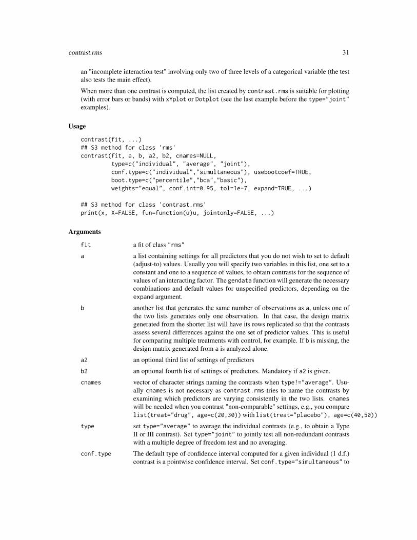
an "incomplete interaction test" involving only two of three levels of a categorical variable (the testalso tests the main effect).
When more than one contrast is computed, the list created by contrast.rms is suitable for plotting(with error bars or bands) with xYplot or Dotplot (see the last example before the type="joint"examples).
Usage
contrast(fit, ...)## S3 method for class 'rms'contrast(fit, a, b, a2, b2, cnames=NULL,
type=c("individual", "average", "joint"),conf.type=c("individual","simultaneous"), usebootcoef=TRUE,boot.type=c("percentile","bca","basic"),weights="equal", conf.int=0.95, tol=1e-7, expand=TRUE, ...)
## S3 method for class 'contrast.rms'print(x, X=FALSE, fun=function(u)u, jointonly=FALSE, ...)
Arguments
fit a fit of class "rms"
a a list containing settings for all predictors that you do not wish to set to default(adjust-to) values. Usually you will specify two variables in this list, one set to aconstant and one to a sequence of values, to obtain contrasts for the sequence ofvalues of an interacting factor. The gendata function will generate the necessarycombinations and default values for unspecified predictors, depending on theexpand argument.
b another list that generates the same number of observations as a, unless one ofthe two lists generates only one observation. In that case, the design matrixgenerated from the shorter list will have its rows replicated so that the contrastsassess several differences against the one set of predictor values. This is usefulfor comparing multiple treatments with control, for example. If b is missing, thedesign matrix generated from a is analyzed alone.
a2 an optional third list of settings of predictors
b2 an optional fourth list of settings of predictors. Mandatory if a2 is given.
cnames vector of character strings naming the contrasts when type!="average". Usu-ally cnames is not necessary as contrast.rms tries to name the contrasts byexamining which predictors are varying consistently in the two lists. cnameswill be needed when you contrast "non-comparable" settings, e.g., you comparelist(treat="drug", age=c(20,30)) with list(treat="placebo"), age=c(40,50))
type set type="average" to average the individual contrasts (e.g., to obtain a TypeII or III contrast). Set type="joint" to jointly test all non-redundant contrastswith a multiple degree of freedom test and no averaging.
conf.type The default type of confidence interval computed for a given individual (1 d.f.)contrast is a pointwise confidence interval. Set conf.type="simultaneous" to
32 contrast.rms
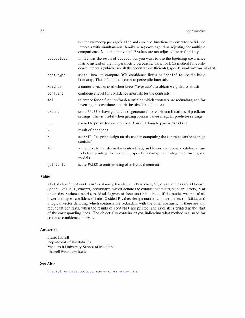
use the multcomp package’s glht and confint functions to compute confidenceintervals with simultaneous (family-wise) coverage, thus adjusting for multiplecomparisons. Note that individual P-values are not adjusted for multiplicity.
usebootcoef If fit was the result of bootcov but you want to use the bootstrap covariancematrix instead of the nonparametric percentile, basic, or BCa method for confi-dence intervals (which uses all the bootstrap coefficients), specify usebootcoef=FALSE.
boot.type set to 'bca' to compute BCa confidence limits or 'basic' to use the basicbootstrap. The default is to compute percentile intervals
weights a numeric vector, used when type="average", to obtain weighted contrasts
conf.int confidence level for confidence intervals for the contrasts
tol tolerance for qr function for determining which contrasts are redundant, and forinverting the covariance matrix involved in a joint test
expand set to FALSE to have gendata not generate all possible combinations of predictorsettings. This is useful when getting contrasts over irregular predictor settings.
... passed to print for main output. A useful thing to pass is digits=4.
x result of contrast
X set X=TRUE to print design matrix used in computing the contrasts (or the averagecontrast)
fun a function to transform the contrast, SE, and lower and upper confidence lim-its before printing. For example, specify fun=exp to anti-log them for logisticmodels.
jointonly set to FALSE to omit printing of individual contrasts
Value
a list of class "contrast.rms" containing the elements Contrast, SE, Z, var, df.residual Lower,Upper, Pvalue, X, cnames, redundant, which denote the contrast estimates, standard errors, Z ort-statistics, variance matrix, residual degrees of freedom (this is NULL if the model was not ols),lower and upper confidence limits, 2-sided P-value, design matrix, contrast names (or NULL), anda logical vector denoting which contrasts are redundant with the other contrasts. If there are anyredundant contrasts, when the results of contrast are printed, and asterisk is printed at the startof the corresponding lines. The object also contains ctype indicating what method was used forcompute confidence intervals.
Author(s)
Frank HarrellDepartment of BiostatisticsVanderbilt University School of [email protected]
See Also
Predict, gendata, bootcov, summary.rms, anova.rms,
contrast.rms 33
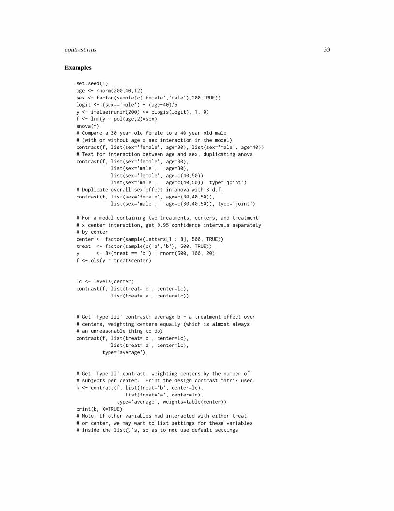
Examples
set.seed(1)age <- rnorm(200,40,12)sex <- factor(sample(c('female','male'),200,TRUE))logit <- (sex=='male') + (age-40)/5y <- ifelse(runif(200) <= plogis(logit), 1, 0)f <- lrm(y ~ pol(age,2)*sex)anova(f)# Compare a 30 year old female to a 40 year old male# (with or without age x sex interaction in the model)contrast(f, list(sex='female', age=30), list(sex='male', age=40))# Test for interaction between age and sex, duplicating anovacontrast(f, list(sex='female', age=30),
list(sex='male', age=30),list(sex='female', age=c(40,50)),list(sex='male', age=c(40,50)), type='joint')
# Duplicate overall sex effect in anova with 3 d.f.contrast(f, list(sex='female', age=c(30,40,50)),
list(sex='male', age=c(30,40,50)), type='joint')
# For a model containing two treatments, centers, and treatment# x center interaction, get 0.95 confidence intervals separately# by centercenter <- factor(sample(letters[1 : 8], 500, TRUE))treat <- factor(sample(c('a','b'), 500, TRUE))y <- 8*(treat == 'b') + rnorm(500, 100, 20)f <- ols(y ~ treat*center)
lc <- levels(center)contrast(f, list(treat='b', center=lc),
list(treat='a', center=lc))
# Get 'Type III' contrast: average b - a treatment effect over# centers, weighting centers equally (which is almost always# an unreasonable thing to do)contrast(f, list(treat='b', center=lc),
list(treat='a', center=lc),type='average')
# Get 'Type II' contrast, weighting centers by the number of# subjects per center. Print the design contrast matrix used.k <- contrast(f, list(treat='b', center=lc),
list(treat='a', center=lc),type='average', weights=table(center))
print(k, X=TRUE)# Note: If other variables had interacted with either treat# or center, we may want to list settings for these variables# inside the list()'s, so as to not use default settings
34 contrast.rms
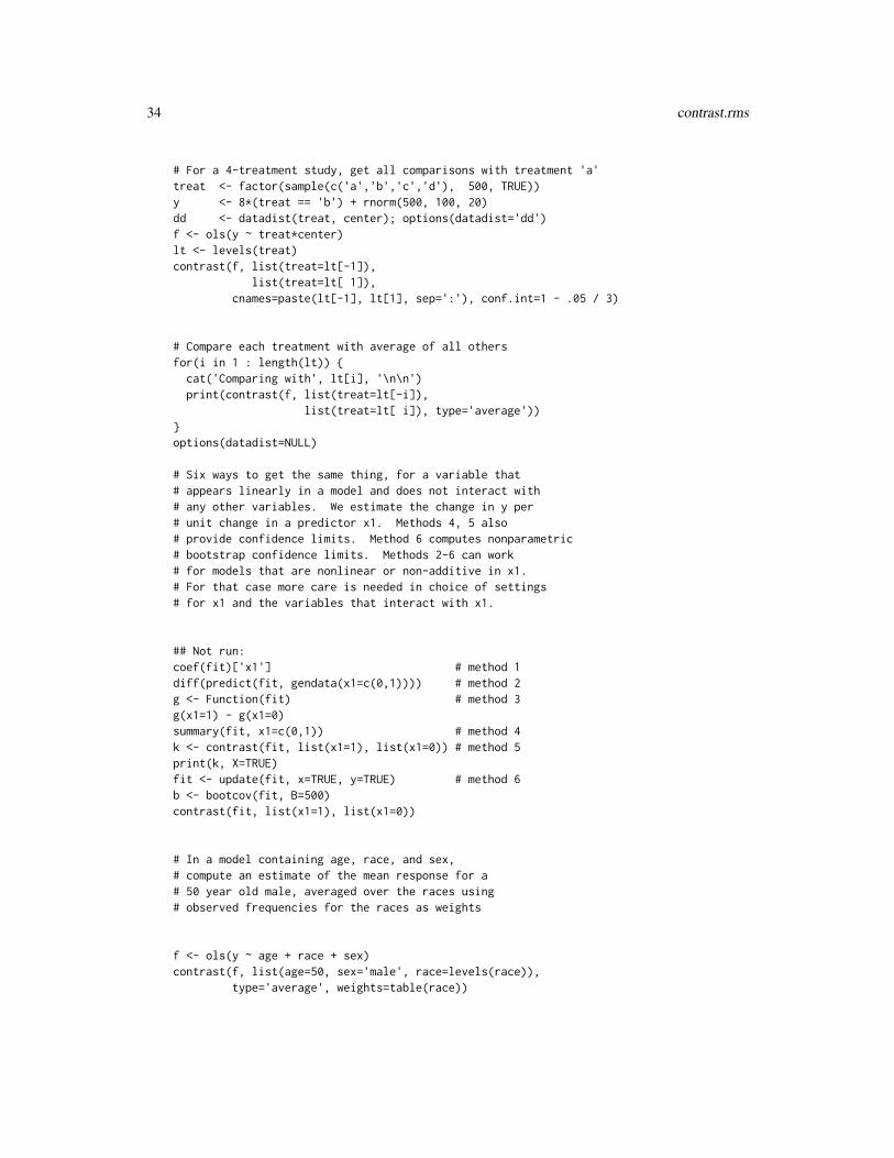
# For a 4-treatment study, get all comparisons with treatment 'a'treat <- factor(sample(c('a','b','c','d'), 500, TRUE))y <- 8*(treat == 'b') + rnorm(500, 100, 20)dd <- datadist(treat, center); options(datadist='dd')f <- ols(y ~ treat*center)lt <- levels(treat)contrast(f, list(treat=lt[-1]),
list(treat=lt[ 1]),cnames=paste(lt[-1], lt[1], sep=':'), conf.int=1 - .05 / 3)
# Compare each treatment with average of all othersfor(i in 1 : length(lt)) {
cat('Comparing with', lt[i], '\n\n')print(contrast(f, list(treat=lt[-i]),
list(treat=lt[ i]), type='average'))}options(datadist=NULL)
# Six ways to get the same thing, for a variable that# appears linearly in a model and does not interact with# any other variables. We estimate the change in y per# unit change in a predictor x1. Methods 4, 5 also# provide confidence limits. Method 6 computes nonparametric# bootstrap confidence limits. Methods 2-6 can work# for models that are nonlinear or non-additive in x1.# For that case more care is needed in choice of settings# for x1 and the variables that interact with x1.
## Not run:coef(fit)['x1'] # method 1diff(predict(fit, gendata(x1=c(0,1)))) # method 2g <- Function(fit) # method 3g(x1=1) - g(x1=0)summary(fit, x1=c(0,1)) # method 4k <- contrast(fit, list(x1=1), list(x1=0)) # method 5print(k, X=TRUE)fit <- update(fit, x=TRUE, y=TRUE) # method 6b <- bootcov(fit, B=500)contrast(fit, list(x1=1), list(x1=0))
# In a model containing age, race, and sex,# compute an estimate of the mean response for a# 50 year old male, averaged over the races using# observed frequencies for the races as weights
f <- ols(y ~ age + race + sex)contrast(f, list(age=50, sex='male', race=levels(race)),
type='average', weights=table(race))
contrast.rms 35
## End(Not run)
# Plot the treatment effect (drug - placebo) as a function of age# and sex in a model in which age nonlinearly interacts with treatment# for females only
set.seed(1)n <- 800treat <- factor(sample(c('drug','placebo'), n,TRUE))sex <- factor(sample(c('female','male'), n,TRUE))age <- rnorm(n, 50, 10)y <- .05*age + (sex=='female')*(treat=='drug')*.05*abs(age-50) + rnorm(n)f <- ols(y ~ rcs(age,4)*treat*sex)d <- datadist(age, treat, sex); options(datadist='d')
# show separate estimates by treatment and sex
ggplot(Predict(f, age, treat, sex='female'))ggplot(Predict(f, age, treat, sex='male'))ages <- seq(35,65,by=5); sexes <- c('female','male')w <- contrast(f, list(treat='drug', age=ages, sex=sexes),
list(treat='placebo', age=ages, sex=sexes))# add conf.type="simultaneous" to adjust for having done 14 contrastsxYplot(Cbind(Contrast, Lower, Upper) ~ age | sex, data=w,
ylab='Drug - Placebo')w <- as.data.frame(w[c('age','sex','Contrast','Lower','Upper')])ggplot(w, aes(x=age, y=Contrast)) + geom_point() + facet_grid(sex ~ .) +
geom_errorbar(aes(ymin=Lower, ymax=Upper), width=0)xYplot(Cbind(Contrast, Lower, Upper) ~ age, groups=sex, data=w,
ylab='Drug - Placebo', method='alt bars')options(datadist=NULL)
# Examples of type='joint' contrast tests
set.seed(1)x1 <- rnorm(100)x2 <- factor(sample(c('a','b','c'), 100, TRUE))dd <- datadist(x1, x2); options(datadist='dd')y <- x1 + (x2=='b') + rnorm(100)
# First replicate a test statistic from anova()
f <- ols(y ~ x2)anova(f)contrast(f, list(x2=c('b','c')), list(x2='a'), type='joint')
# Repeat with a redundancy; compare a vs b, a vs c, b vs c
contrast(f, list(x2=c('a','a','b')), list(x2=c('b','c','c')), type='joint')
36 cph
# Get a test of association of a continuous predictor with y# First assume linearity, then cubic
f <- lrm(y>0 ~ x1 + x2)anova(f)contrast(f, list(x1=1), list(x1=0), type='joint') # a minimum set of contrastsxs <- seq(-2, 2, length=20)contrast(f, list(x1=0), list(x1=xs), type='joint')
# All contrasts were redundant except for the first, because of# linearity assumption
f <- lrm(y>0 ~ pol(x1,3) + x2)anova(f)contrast(f, list(x1=0), list(x1=xs), type='joint')print(contrast(f, list(x1=0), list(x1=xs), type='joint'), jointonly=TRUE)
# All contrasts were redundant except for the first 3, because of# cubic regression assumption
# Now do something that is difficult to do without cryptic contrast# matrix operations: Allow each of the three x2 groups to have a different# shape for the x1 effect where x1 is quadratic. Test whether there is# a difference in mean levels of y for x2='b' vs. 'c' or whether# the shape or slope of x1 is different between x2='b' and x2='c' regardless# of how they differ when x2='a'. In other words, test whether the mean# response differs between group b and c at any value of x1.# This is a 3 d.f. test (intercept, linear, quadratic effects) and is# a better approach than subsetting the data to remove x2='a' then# fitting a simpler model, as it uses a better estimate of sigma from# all the data.
f <- ols(y ~ pol(x1,2) * x2)anova(f)contrast(f, list(x1=xs, x2='b'),
list(x1=xs, x2='c'), type='joint')
# Note: If using a spline fit, there should be at least one value of# x1 between any two knots and beyond the outer knots.options(datadist=NULL)
cph Cox Proportional Hazards Model and Extensions
Description
Modification of Therneau’s coxph function to fit the Cox model and its extension, the Andersen-Gill model. The latter allows for interval time-dependent covariables, time-dependent strata, andrepeated events. The Survival method for an object created by cph returns an S function forcomputing estimates of the survival function. The Quantile method for cph returns an S function
cph 37
for computing quantiles of survival time (median, by default). The Mean method returns a functionfor computing the mean survival time. This function issues a warning if the last follow-up time isuncensored, unless a restricted mean is explicitly requested.
Usage
cph(formula = formula(data), data=parent.frame(),weights, subset, na.action=na.delete,method=c("efron","breslow","exact","model.frame","model.matrix"),singular.ok=FALSE, robust=FALSE,model=FALSE, x=FALSE, y=FALSE, se.fit=FALSE,linear.predictors=TRUE, residuals=TRUE, nonames=FALSE,eps=1e-4, init, iter.max=10, tol=1e-9, surv=FALSE, time.inc,type=NULL, vartype=NULL, debug=FALSE, ...)
## S3 method for class 'cph'Survival(object, ...)# Evaluate result as g(times, lp, stratum=1, type=c("step","polygon"))
## S3 method for class 'cph'Quantile(object, ...)# Evaluate like h(q, lp, stratum=1, type=c("step","polygon"))
## S3 method for class 'cph'Mean(object, method=c("exact","approximate"), type=c("step","polygon"),
n=75, tmax, ...)# E.g. m(lp, stratum=1, type=c("step","polygon"), tmax, ...)
Arguments
formula an S formula object with a Surv object on the left-hand side. The terms canspecify any S model formula with up to third-order interactions. The stratfunction may appear in the terms, as a main effect or an interacting factor. Tostratify on both race and sex, you would include both terms strat(race) andstrat(sex). Stratification factors may interact with non-stratification factors;not all stratification terms need interact with the same modeled factors.
object an object created by cph with surv=TRUE
data name of an S data frame containing all needed variables. Omit this to use a dataframe already in the S “search list”.
weights case weights
subset an expression defining a subset of the observations to use in the fit. The de-fault is to use all observations. Specify for example age>50 & sex="male"or c(1:100,200:300) respectively to use the observations satisfying a logicalexpression or those having row numbers in the given vector.
na.action specifies an S function to handle missing data. The default is the functionna.delete, which causes observations with any variable missing to be deleted.The main difference between na.delete and the S-supplied function na.omit
38 cph
is that na.delete makes a list of the number of observations that are miss-ing on each variable in the model. The na.action is usally specified by e.g.options(na.action="na.delete").
method for cph, specifies a particular fitting method, "model.frame" instead to returnthe model frame of the predictor and response variables satisfying any subset ormissing value checks, or "model.matrix" to return the expanded design matrix.The default is "efron", to use Efron’s likelihood for fitting the model.For Mean.cph, method is "exact" to use numerical integration of the survivalfunction at any linear predictor value to obtain a mean survival time. Spec-ify method="approximate" to use an approximate method that is slower whenMean.cph is executing but then is essentially instant thereafter. For the approxi-mate method, the area is computed for n points equally spaced between the minand max observed linear predictor values. This calculation is done separately foreach stratum. Then the n pairs (X beta, area) are saved in the generated S func-tion, and when this function is evaluated, the approx function is used to evaluatethe mean for any given linear predictor values, using linear interpolation over then X beta values.
singular.ok If TRUE, the program will automatically skip over columns of the X matrix thatare linear combinations of earlier columns. In this case the coefficients for suchcolumns will be NA, and the variance matrix will contain zeros. For ancillarycalculations, such as the linear predictor, the missing coefficients are treated aszeros. The singularities will prevent many of the features of the rms library fromworking.
robust if TRUE a robust variance estimate is returned. Default is TRUE if the modelincludes a cluster() operative, FALSE otherwise.
model default is FALSE(false). Set to TRUE to return the model frame as element modelof the fit object.
x default is FALSE. Set to TRUE to return the expanded design matrix as element x(without intercept indicators) of the returned fit object.
y default is FALSE. Set to TRUE to return the vector of response values (Surv object)as element y of the fit.
se.fit default is FALSE. Set to TRUE to compute the estimated standard errors of theestimate of X beta and store them in element se.fit of the fit. The predictorsare first centered to their means before computing the standard errors.
linear.predictors
set to FALSE to omit linear.predictors vector from fit
residuals set to FALSE to omit residuals vector from fit
nonames set to TRUE to not set names attribute for linear.predictors, residuals,se.fit, and rows of design matrix
eps convergence criterion - change in log likelihood.
init vector of initial parameter estimates. Defaults to all zeros. Special residuals canbe obtained by setting some elements of init to MLEs and others to zero andspecifying iter.max=1.
iter.max maximum number of iterations to allow. Set to 0 to obtain certain null-modelresiduals.
cph 39
tol tolerance for declaring singularity for matrix inversion (available only when sur-vival5 or later package is in effect)
surv set to TRUE to compute underlying survival estimates for each stratum, and tostore these along with standard errors of log Lambda(t), maxtime (maximumobserved survival or censoring time), and surv.summary in the returned object.Set surv="summary" to only compute and store surv.summary, not survivalestimates at each unique uncensored failure time. If you specify x=TRUE andy=TRUE, you can obtain predicted survival later, with accurate confidence inter-vals for any set of predictor values. The standard error information stored as aresult of surv=TRUE are only accurate at the mean of all predictors. If the modelhas no covariables, these are of course OK. The main reason for using survis to greatly speed up the computation of predicted survival probabilities as afunction of the covariables, when accurate confidence intervals are not needed.
time.inc time increment used in deriving surv.summary. Survival, number at risk, andstandard error will be stored for t=0, time.inc, 2 time.inc, ..., maxtime,where maxtime is the maximum survival time over all strata. time.inc is alsoused in constructing the time axis in the survplot function (see below). Thedefault value for time.inc is 30 if units(ftime) = "Day" or no units at-tribute has been attached to the survival time variable. If units(ftime) is aword other than "Day", the default for time.inc is 1 when it is omitted, unlessmaxtime<1, then maxtime/10 is used as time.inc. If time.inc is not givenand maxtime/ default time.inc > 25, time.inc is increased.
type (for cph) applies if surv is TRUE or "summary". If type is omitted, the methodconsistent with method is used. See survfit.coxph (under survfit) or survfit.cphfor details and for the definitions of values of typeFor Survival, Quantile, Mean set to "polygon" to use linear interpolationinstead of the usual step function. For Mean, the default of step will yield thesample mean in the case of no censoring and no covariables, if type="kaplan-meier"was specified to cph. For method="exact", the value of type is passed to thegenerated function, and it can be overridden when that function is actually in-voked. For method="approximate", Mean.cph generates the function differentways according to type, and this cannot be changed when the function is actu-ally invoked.
vartype see survfit.coxph
debug set to TRUE to print debugging information related to model matrix construction.You can also use options(debug=TRUE).
... other arguments passed to coxph.fit from cph. Ignored by other functions.
times a scalar or vector of times at which to evaluate the survival estimates
lp a scalar or vector of linear predictors (including the centering constant) at whichto evaluate the survival estimates
stratum a scalar stratum number or name (e.g., "sex=male") to use in getting survivalprobabilities
q a scalar quantile or a vector of quantiles to compute
n the number of points at which to evaluate the mean survival time, for method="approximate"in Mean.cph.

40 cph
tmax For Mean.cph, the default is to compute the overall mean (and produce a warn-ing message if there is censoring at the end of follow-up). To compute a re-stricted mean life length, specify the truncation point as tmax. For method="exact",tmax is passed to the generated function and it may be overridden when thatfunction is invoked. For method="approximate", tmax must be specified at thetime that Mean.cph is run.
Details
If there is any strata by covariable interaction in the model such that the mean X beta variesgreatly over strata, method="approximate" may not yield very accurate estimates of the meanin Mean.cph.
For method="approximate" if you ask for an estimate of the mean for a linear predictor value thatwas outside the range of linear predictors stored with the fit, the mean for that observation will beNA.
Value
For Survival, Quantile, or Mean, an S function is returned. Otherwise, in addition to what is listedbelow, formula/design information and the components maxtime, time.inc, units, model, x, y, se.fitare stored, the last 5 depending on the settings of options by the same names. The vectors or matrixstored if y=TRUE or x=TRUE have rows deleted according to subset and to missing data, and havenames or row names that come from the data frame used as input data.
n table with one row per stratum containing number of censored and uncensoredobservations
coef vector of regression coefficients
stats vector containing the named elements Obs, Events, Model L.R., d.f., P,Score, Score P, R2, Somers’ Dxy, g-index, and gr, the g-index on the haz-ard ratio scale. R2 is the Nagelkerke R-squared, with division by the maximumattainable R-squared.
var variance/covariance matrix of coefficientslinear.predictors
values of predicted X beta for observations used in fit, normalized to have overallmean zero, then having any offsets added
resid martingale residuals
loglik log likelihood at initial and final parameter values
score value of score statistic at initial values of parameters
times lists of times (if surv="T")
surv lists of underlying survival probability estimates
std.err lists of standard errors of estimate log-log survival
surv.summary a 3 dimensional array if surv=TRUE. The first dimension is time ranging from0 to maxtime by time.inc. The second dimension refers to strata. The thirddimension contains the time-oriented matrix with Survival, n.risk (numberof subjects at risk), and std.err (standard error of log-log survival).
center centering constant, equal to overall mean of X beta.
cph 41
Author(s)
Frank HarrellDepartment of Biostatistics, Vanderbilt University<[email protected]>
See Also
coxph, survival-internal, Surv, residuals.cph, cox.zph, survfit.cph, survest.cph, survfit.coxph,survplot, datadist, rms, rms.trans, anova.rms, summary.rms, Predict, fastbw, validate,calibrate, plot.Predict, ggplot.Predict, specs.rms, lrm, which.influence, na.delete,na.detail.response, print.cph, latex.cph, vif, ie.setup, GiniMd, dxy.cens, survConcordance
Examples
# Simulate data from a population model in which the log hazard# function is linear in age and there is no age x sex interaction
n <- 1000set.seed(731)age <- 50 + 12*rnorm(n)label(age) <- "Age"sex <- factor(sample(c('Male','Female'), n,
rep=TRUE, prob=c(.6, .4)))cens <- 15*runif(n)h <- .02*exp(.04*(age-50)+.8*(sex=='Female'))dt <- -log(runif(n))/hlabel(dt) <- 'Follow-up Time'e <- ifelse(dt <= cens,1,0)dt <- pmin(dt, cens)units(dt) <- "Year"dd <- datadist(age, sex)options(datadist='dd')S <- Surv(dt,e)
f <- cph(S ~ rcs(age,4) + sex, x=TRUE, y=TRUE)cox.zph(f, "rank") # tests of PHanova(f)ggplot(Predict(f, age, sex)) # plot age effect, 2 curves for 2 sexessurvplot(f, sex) # time on x-axis, curves for x2res <- resid(f, "scaledsch")time <- as.numeric(dimnames(res)[[1]])z <- loess(res[,4] ~ time, span=0.50) # residuals for sexplot(time, fitted(z))lines(supsmu(time, res[,4]),lty=2)plot(cox.zph(f,"identity")) #Easier approach for last few lines# latex(f)
f <- cph(S ~ age + strat(sex), surv=TRUE)g <- Survival(f) # g is a functiong(seq(.1,1,by=.1), stratum="sex=Male", type="poly") #could use stratum=2
42 cph
med <- Quantile(f)plot(Predict(f, age, fun=function(x) med(lp=x))) #plot median survival
# Fit a model that is quadratic in age, interacting with sex as strata# Compare standard errors of linear predictor values with those from# coxph# Use more stringent convergence criteria to match with coxph
f <- cph(S ~ pol(age,2)*strat(sex), x=TRUE, eps=1e-9, iter.max=20)coef(f)se <- predict(f, se.fit=TRUE)$se.fitrequire(lattice)xyplot(se ~ age | sex, main='From cph')a <- c(30,50,70)comb <- data.frame(age=rep(a, each=2),
sex=rep(levels(sex), 3))
p <- predict(f, comb, se.fit=TRUE)comb$yhat <- p$linear.predictorscomb$se <- p$se.fitz <- qnorm(.975)comb$lower <- p$linear.predictors - z*p$se.fitcomb$upper <- p$linear.predictors + z*p$se.fitcomb
age2 <- age^2f2 <- coxph(S ~ (age + age2)*strata(sex))coef(f2)se <- predict(f2, se.fit=TRUE)$se.fitxyplot(se ~ age | sex, main='From coxph')comb <- data.frame(age=rep(a, each=2), age2=rep(a, each=2)^2,
sex=rep(levels(sex), 3))p <- predict(f2, newdata=comb, se.fit=TRUE)comb$yhat <- p$fitcomb$se <- p$se.fitcomb$lower <- p$fit - z*p$se.fitcomb$upper <- p$fit + z*p$se.fitcomb
# g <- cph(Surv(hospital.charges) ~ age, surv=TRUE)# Cox model very useful for analyzing highly skewed data, censored or not# m <- Mean(g)# m(0) # Predicted mean charge for reference age
#Fit a time-dependent covariable representing the instantaneous effect#of an intervening non-fatal eventrm(age)set.seed(121)dframe <- data.frame(failure.time=1:10, event=rep(0:1,5),
ie.time=c(NA,1.5,2.5,NA,3,4,NA,5,5,5),age=sample(40:80,10,rep=TRUE))
cr.setup 43
z <- ie.setup(dframe$failure.time, dframe$event, dframe$ie.time)S <- z$Sie.status <- z$ie.statusattach(dframe[z$subs,]) # replicates all variables
f <- cph(S ~ age + ie.status, x=TRUE, y=TRUE)#Must use x=TRUE,y=TRUE to get survival curves with time-dep. covariables
#Get estimated survival curve for a 50-year old who has an intervening#non-fatal event at 5 daysnew <- data.frame(S=Surv(c(0,5), c(5,999), c(FALSE,FALSE)), age=rep(50,2),
ie.status=c(0,1))g <- survfit(f, new)plot(c(0,g$time), c(1,g$surv[,2]), type='s',
xlab='Days', ylab='Survival Prob.')# Not certain about what columns represent in g$surv for survival5# but appears to be for different ie.status#or:#g <- survest(f, new)#plot(g$time, g$surv, type='s', xlab='Days', ylab='Survival Prob.')
#Compare with estimates when there is no intervening eventnew2 <- data.frame(S=Surv(c(0,5), c(5, 999), c(FALSE,FALSE)), age=rep(50,2),
ie.status=c(0,0))g2 <- survfit(f, new2)lines(c(0,g2$time), c(1,g2$surv[,2]), type='s', lty=2)#or:#g2 <- survest(f, new2)#lines(g2$time, g2$surv, type='s', lty=2)detach("dframe[z$subs, ]")options(datadist=NULL)
cr.setup Continuation Ratio Ordinal Logistic Setup
Description
Creates several new variables which help set up a dataset with an ordinal response variable y for usein fitting a forward continuation ratio (CR) model. The CR model can be fitted with binary logisticregression if each input observation is replicated the proper number of times according to the yvalue, a new binary y is computed that has at most one y = 1 per subject, and if a cohort variableis used to define the current qualifying condition for a cohort of subjects, e.g., y ≥ 2. cr.setupcreates the needed auxilliary variables. See predab.resample and validate.lrm for informationabout validating CR models (e.g., using the bootstrap to sample with replacement from the originalsubjects instead of the records used in the fit, validating the model separately for user-specifiedvalues of cohort).
44 cr.setup
Usage
cr.setup(y)
Arguments
y a character, numeric, category, or factor vector containing values of the re-sponse variable. For category or factor variables, the levels of the variableare assumed to be listed in an ordinal way.
Value
a list with components y, cohort, subs, reps. y is a new binary variable that is to be used in thebinary logistic fit. cohort is a factor vector specifying which cohort condition currently applies.subs is a vector of subscripts that can be used to replicate other variables the same way y was repli-cated. reps specifies how many times each original observation was replicated. y, cohort, subsare all the same length and are longer than the original y vector. reps is the same length as the orig-inal y vector. The subs vector is suitable for passing to validate.lrm or calibrate, which passthis vector under the name cluster on to predab.resample so that bootstrapping can be doneby sampling with replacement from the original subjects rather than from the individual recordscreated by cr.setup.
Author(s)
Frank HarrellDepartment of BiostatisticsVanderbilt [email protected]
References
Berridge DM, Whitehead J: Analysis of failure time data with ordinal categories of response. Statin Med 10:1703–1710, 1991.
See Also
lrm, glm, predab.resample
Examples
y <- c(NA, 10, 21, 32, 32)cr.setup(y)
set.seed(171)y <- sample(0:2, 100, rep=TRUE)sex <- sample(c("f","m"),100,rep=TRUE)sex <- factor(sex)table(sex, y)options(digits=5)tapply(y==0, sex, mean)
cr.setup 45
tapply(y==1, sex, mean)tapply(y==2, sex, mean)cohort <- y>=1tapply(y[cohort]==1, sex[cohort], mean)
u <- cr.setup(y)Y <- u$ycohort <- u$cohortsex <- sex[u$subs]
lrm(Y ~ cohort + sex)
f <- lrm(Y ~ cohort*sex) # saturated model - has to fit all data cellsf
#Prob(y=0|female):# plogis(-.50078)#Prob(y=0|male):# plogis(-.50078+.11301)#Prob(y=1|y>=1, female):plogis(-.50078+.31845)#Prob(y=1|y>=1, male):plogis(-.50078+.31845+.11301-.07379)
combinations <- expand.grid(cohort=levels(cohort), sex=levels(sex))combinationsp <- predict(f, combinations, type="fitted")pp0 <- p[c(1,3)]p1 <- p[c(2,4)]p1.unconditional <- (1 - p0) *p1p1.unconditionalp2.unconditional <- 1 - p0 - p1.unconditionalp2.unconditional
## Not run:dd <- datadist(inputdata) # do this on non-replicated dataoptions(datadist='dd')pain.severity <- inputdata$pain.severityu <- cr.setup(pain.severity)# inputdata frame has age, sex with pain.severityattach(inputdata[u$subs,]) # replicate age, sex# If age, sex already available, could do age <- age[u$subs] etc., or# age <- rep(age, u$reps), etc.y <- u$ycohort <- u$cohortdd <- datadist(dd, cohort) # add to ddf <- lrm(y ~ cohort + age*sex) # ordinary cont. ratio modelg <- lrm(y ~ cohort*sex + age, x=TRUE,y=TRUE) # allow unequal slopes for
# sex across cutoffscal <- calibrate(g, cluster=u$subs, subset=cohort=='all')# subs makes bootstrap sample the correct units, subset causes
46 datadist
# Predicted Prob(pain.severity=0) to be checked for calibration
## End(Not run)
datadist Distribution Summaries for Predictor Variables
Description
For a given set of variables or a data frame, determines summaries of variables for effect and plot-ting ranges, values to adjust to, and overall ranges for Predict, plot.Predict, ggplot.Predict,summary.rms, survplot, and nomogram.rms. If datadist is called before a model fit and the re-sulting object pointed to with options(datadist="name"), the data characteristics will be storedwith the fit by Design(), so that later predictions and summaries of the fit will not need to accessthe original data used in the fit. Alternatively, you can specify the values for each variable in themodel when using these 3 functions, or specify the values of some of them and let the functions lookup the remainder (of say adjustmemt levels) from an object created by datadist. The best methodis probably to run datadist once before any models are fitted, storing the distribution summariesfor all potential variables. Adjustment values are 0 for binary variables, the most frequent cate-gory (or optionally the first category level) for categorical (factor) variables, the middle level forordered factor variables, and medians for continuous variables. See descriptions of q.displayand q.effect for how display and effect ranges are chosen for continuous variables.
Usage
datadist(..., data, q.display, q.effect=c(0.25, 0.75),adjto.cat=c('mode','first'), n.unique=10)
## S3 method for class 'datadist'print(x, ...)# options(datadist="dd")# used by summary, plot, survplot, sometimes predict# For dd substitute the name of the result of datadist
Arguments
... a list of variable names, separated by commas, a single data frame, or a fit withDesign information. The first element in this list may also be an object cre-ated by an earlier call to datadist; then the later variables are added to thisdatadist object. For a fit object, the variables named in the fit are retrievedfrom the active data frame or from the location pointed to by data=frame numberor data="data frame name". For print, is ignored.
data a data frame or a search position. If data is a search position, it is assumed thata data frame is attached in that position, and all its variables are used. If youspecify both individual variables in ... and data, the two sets of variables arecombined. Unless the first argument is a fit object, data must be an integer.

datadist 47
q.display set of two quantiles for computing the range of continuous variables to usein displaying regression relationships. Defaults are q and 1 − q, where q =10/max(n, 200), and n is the number of non-missing observations. Thus forn < 200, the .05 and .95 quantiles are used. For n ≥ 200, the 10th smallest and10th largest values are used. If you specify q.display, those quantiles are usedwhether or not n < 200.
q.effect set of two quantiles for computing the range of continuous variables to use in es-timating regression effects. Defaults are c(.25,.75), which yields inter-quartile-range odds ratios, etc.
adjto.cat default is "mode", indicating that the modal (most frequent) category for cat-egorical (factor) variables is the adjust-to setting. Specify "first" to use thefirst level of factor variables as the adjustment values. In the case of many levelshaving the maximum frequency, the first such level is used for "mode".
n.unique variables having n.unique or fewer unique values are considered to be discretevariables in that their unique values are stored in the values list. This willaffect how functions such as nomogram.Design determine whether variablesare discrete or not.
x result of datadist
Details
For categorical variables, the 7 limits are set to character strings (factors) which correspond toc(NA,adjto.level,NA,1,k,1,k), where k is the number of levels. For ordered variables withnumeric levels, the limits are set to c(L,M,H,L,H,L,H), where L is the lowest level, M is the middlelevel, and H is the highest level.
Value
a list of class "datadist" with the following components
limits a 7 × k vector, where k is the number of variables. The 7 rows correspondto the low value for estimating the effect of the variable, the value to adjustthe variable to when examining other variables, the high value for effect, lowvalue for displaying the variable, the high value for displaying it, and the overalllowest and highest values.
values a named list, with one vector of unique values for each numeric variable havingno more than n.unique unique values
Author(s)
Frank HarrellDepartment of BiostatisticsVanderbilt [email protected]
See Also
rms, rms.trans, describe, Predict, summary.rms
48 ExProb
Examples
## Not run:d <- datadist(data=1) # use all variables in search pos. 1d <- datadist(x1, x2, x3)page(d) # if your options(pager) leaves up a pop-up
# window, this is a useful guide in analysesd <- datadist(data=2) # all variables in search pos. 2d <- datadist(data=my.data.frame)d <- datadist(my.data.frame) # same as previous. Run for all potential vars.d <- datadist(x2, x3, data=my.data.frame) # combine variablesd <- datadist(x2, x3, q.effect=c(.1,.9), q.display=c(0,1))# uses inter-decile range odds ratios,# total range of variables for regression function plotsd <- datadist(d, z) # add a new variable to an existing datadistoptions(datadist="d") #often a good idea, to store info with fitf <- ols(y ~ x1*x2*x3)
options(datadist=NULL) #default at start of sessionf <- ols(y ~ x1*x2)d <- datadist(f) #info not stored in `f'd$limits["Adjust to","x1"] <- .5 #reset adjustment level to .5options(datadist="d")
f <- lrm(y ~ x1*x2, data=mydata)d <- datadist(f, data=mydata)options(datadist="d")
f <- lrm(y ~ x1*x2) #datadist not used - specify all values forsummary(f, x1=c(200,500,800), x2=c(1,3,5)) # obtaining predictionsplot(Predict(f, x1=200:800, x2=3)) # or ggplot()
# Change reference value to get a relative odds plot for a logistic modeld$limits$age[2] <- 30 # make 30 the reference value for age# Could also do: d$limits["Adjust to","age"] <- 30fit <- update(fit) # make new reference value take effectplot(Predict(fit, age, ref.zero=TRUE, fun=exp),
ylab='Age=x:Age=30 Odds Ratio') # or ggplot()
## End(Not run)
ExProb Function Generator For Exceedance Probabilities
Description
For an orm object generates a function for computing the estimates of the function Prob(Y>=y)given one or more values of the linear predictor using the reference (median) intercept. This function
ExProb 49
can optionally be evaluated at only a set of user-specified y values, otherwise a right-step function isreturned. There is a plot method for plotting the step functions, and if more than one linear predictorwas evaluated multiple step functions are drawn. ExProb is especially useful for nomogram.
Usage
ExProb(object, ...)
## S3 method for class 'orm'ExProb(object, codes = FALSE, ...)
## S3 method for class 'ExProb'plot(x, ..., data=NULL,
xlim=NULL, xlab=x$yname, ylab=expression(Prob(Y>=y)),col=par('col'), col.vert='gray85', pch=20,pch.data=21, lwd=par('lwd'), lwd.data=lwd,lty.data=2, key=TRUE)
Arguments
object a fit object from orm
codes if TRUE, ExProb use the integer codes 1, 2, . . . , k for the k-level response insteadof its original unique values
... ignored for ExProb. Passed to plot for plot.ExProb
data Specify data if you want to add stratified empirical probabilities to the graph.If data is a numeric vector, it is assumed that no groups are present. Otherwisedata must be a list or data frame where the first variable is the grouping variable(corresponding to what made the linear predictor vary) and the second variableis the data vector for the y variable. The rows of data should be sorted to be inorder of the linear predictor argument.
x an object created by running the function created by ExProb
xlim limits for x-axis; default is range of observed y
xlab x-axis label
ylab y-axis label
col color for horizontal lines and points
col.vert color for vertical discontinuities
pch plotting symbol for predicted curves
lwd line width for predicted curvespch.data,lwd.data,lty.data
plotting parameters for data
key set to FALSE to suppress key in plot if data is given
Value
ExProb returns an R function. Running the function returns an object of class "ExProb".

50 fastbw
Author(s)
Frank Harrell
See Also
orm, Quantile.orm
Examples
set.seed(1)x1 <- runif(200)yvar <- x1 + runif(200)f <- orm(yvar ~ x1)d <- ExProb(f)lp <- predict(f, newdata=data.frame(x1=c(.2,.8)))w <- d(lp)s1 <- abs(x1 - .2) < .1s2 <- abs(x1 - .8) < .1plot(w, data=data.frame(x1=c(rep(.2, sum(s1)), rep(.8, sum(s2))),
yvar=c(yvar[s1], yvar[s2])))
qu <- Quantile(f)abline(h=c(.1,.5), col='gray80')abline(v=qu(.5, lp), col='gray80')abline(v=qu(.9, lp), col='green')
fastbw Fast Backward Variable Selection
Description
Performs a slightly inefficient but numerically stable version of fast backward elimination on fac-tors, using a method based on Lawless and Singhal (1978). This method uses the fitted completemodel and computes approximate Wald statistics by computing conditional (restricted) maximumlikelihood estimates assuming multivariate normality of estimates. fastbw deletes factors, notcolumns of the design matrix. Factors requiring multiple d.f. will be retained or dropped as agroup. The function prints the deletion statistics for each variable in turn, and prints approximateparameter estimates for the model after deleting variables. The approximation is better when thenumber of factors deleted is not large. For ols, the approximation is exact for regression coef-ficients, and standard errors are only off by a factor equal to the ratio of the mean squared errorestimate for the reduced model to the original mean squared error estimate for the full model.
If the fit was from ols, fastbw will compute the usual R2 statistic for each model.
Usage
fastbw(fit, rule=c("aic", "p"),type=c("residual", "individual", "total"), sls=.05, aics=0, eps=1e-9,k.aic=2, force=NULL)

fastbw 51
## S3 method for class 'fastbw'print(x, digits=4, estimates=TRUE, ...)
Arguments
fit fit object with Varcov(fit) defined (e.g., from ols, lrm, cph, psm, glmD)
rule Stopping rule. Defaults to "aic" for Akaike’s information criterion. Use rule="p"to use P -values
type Type of statistic on which to base the stopping rule. Default is "residual" forthe pooled residual chi-square. Use type="individual" to use Wald chi-squareof individual factors.
sls Significance level for staying in a model if rule="p". Default is .05.
aics For rule="aic", variables are deleted until the chi-square - k.aic times d.f.would rise above aics. Default aics is zero to use the ordinary AIC. Set aicsto say 10000 to see all variables deleted in order of descending importance.
eps Singularity criterion, default is 1E-9.
k.aic multiplier to compute AIC, default is 2. To use BIC, set k.aic equal to log(n),where n is the effective sample size (number of events for survival models).
force a vector of integers specifying parameters forced to be in the model, not countingintercept(s)
x result of fastbw
digits number of significant digits to print
estimates set to FALSE to suppress printing table of approximate coefficients, SEs, etc.,after variable deletions
... ignored
Value
a list with an attribute kept if bw=TRUE, and the following components:
result matrix of statistics with rows in order of deletion.
names.kept names of factors kept in final model.
factors.kept the subscripts of factors kept in the final modelfactors.deleted
opposite of factors.kept.
parms.kept column numbers in design matrix corresponding to parameters kept in the finalmodel.
parms.deleted opposite of parms.kept.
coefficients vector of approximate coefficients of reduced model.
var approximate covariance matrix for reduced model.
Coefficients matrix of coefficients of all models. Rows correspond to the successive modelsexamined and columns correspond to the coefficients in the full model. Forvariables not in a particular sub-model (row), the coefficients are zero.

52 Function
Author(s)
Frank HarrellDepartment of Biostatistics, Vanderbilt [email protected]
References
Lawless, J. F. and Singhal, K. (1978): Efficient screening of nonnormal regression models. Biomet-rics 34:318–327.
See Also
rms, ols, lrm, cph, psm, validate, solvet, rmsMisc
Examples
## Not run:fastbw(fit, optional.arguments) # print resultsz <- fastbw(fit, optional.args) # typically used in simulationslm.fit(X[,z$parms.kept], Y) # least squares fit of reduced model
## End(Not run)
Function Compose an S Function to Compute X beta from a Fit
Description
Function is a class of functions for creating other S functions. Function.rms is the method forcreating S functions to compute X beta, based on a model fitted with rms in effect. Like latexrms,Function.rms simplifies restricted cubic spline functions and factors out terms in second-orderinteractions. Function.rms will not work for models that have third-order interactions involvingrestricted cubic splines. Function.cph is a particular method for handling fits from cph, for whichan intercept (the negative of the centering constant) is added to the model. sascode is a functionthat takes an S function such as one created by Function and does most of the editing to turn thefunction definition into a fragment of SAS code for computing X beta from the fitted model, alongwith assignment statements that initialize predictors to reference values. perlcode similarly createsPerl code to evaluate a fitted regression model.
Usage
## S3 method for class 'rms'Function(object, intercept=NULL,digits=max(8, .Options$digits), ...)
## S3 method for class 'cph'Function(object, intercept=-object$center, ...)
Function 53
# Use result as fun(predictor1=value1, predictor2=value2, ...)
sascode(object, file='', append=FALSE)
perlcode(object)
Arguments
object a fit created with rms in effect
intercept an intercept value to use (not allowed to be specified to Function.cph). Theintercept is usually retrieved from the regression coefficients automatically.
digits number of significant digits to use for coefficients and knot locations
file name of a file in which to write the SAS code. Default is to write to standardoutput.
append set to TRUE to have sascode append code to an existing file named file.
... arguments to pass to Function.rms from Function.cph
Value
Function returns an S-Plus function that can be invoked in any usual context. The function hasone argument per predictor variable, and the default values of the predictors are set to adjust-tovalues (see datadist). Multiple predicted X beta values may be calculated by specifying vectorsas arguments to the created function. All non-scalar argument values must have the same length.perlcode returns a character string with embedded newline characters.
Author(s)
Frank Harrell, Jeremy Stephens, and Thomas DupontDepartment of BiostatisticsVanderbilt [email protected]
See Also
latexrms, transcan, predict.rms, rms, rms.trans
Examples
set.seed(1331)x1 <- exp(rnorm(100))x2 <- factor(sample(c('a','b'),100,rep=TRUE))dd <- datadist(x1, x2)options(datadist='dd')y <- log(x1)^2+log(x1)*(x2=='b')+rnorm(100)/4f <- ols(y ~ pol(log(x1),2)*x2)f$coefg <- Function(f, digits=5)gsascode(g)
54 gendata
cat(perlcode(g), '\n')g()g(x1=c(2,3), x2='b') #could omit x2 since b is default categorypredict(f, expand.grid(x1=c(2,3),x2='b'))g8 <- Function(f) # default is 8 sig. digitsg8(x1=c(2,3), x2='b')options(datadist=NULL)
## Not run:# Make self-contained functions for computing survival probabilities# using a log-normal regressionf <- psm(Surv(d.time, death) ~ rcs(age,4)*sex, dist='gaussian')g <- Function(f)surv <- Survival(f)# Compute 2 and 5-year survival estimates for 50 year old malesurv(c(2,5), g(age=50, sex='male'))
## End(Not run)
gendata Generate Data Frame with Predictor Combinations
Description
If nobs is not specified, allows user to specify predictor settings by e.g. age=50, sex="male",and any omitted predictors are set to reference values (default=median for continuous variables,first level for categorical ones - see datadist). If any predictor has more than one value given,expand.grid is called to generate all possible combinations of values, unless expand=FALSE. Ifnobs is given, a data frame is first generated which has nobs of adjust-to values duplicated. Thenan editor window is opened which allows the user to subset the variable names down to ones whichshe intends to vary (this streamlines the data.ed step). Then, if any predictors kept are discreteand viewvals=TRUE, a window (using page) is opened defining the possible values of this subset,to facilitate data editing. Then the data.ed function is invoked to allow interactive overriding ofpredictor settings in the nobs rows. The subset of variables are combined with the other predictorswhich were not displayed with data.ed, and a final full data frame is returned. gendata is mostuseful for creating a newdata data frame to pass to predict.
Usage
gendata(fit, ..., nobs, viewvals=FALSE, expand=TRUE, factors)
Arguments
fit a fit object created with rms in effect
... predictor settings, if nobs is not given.
nobs number of observations to create if doing it interactively using X-windows

gendata 55
viewvals if nobs is given, set viewvals=TRUE to open a window displaying the possiblevalue of categorical predictors
expand set to FALSE to prevent expand.grid from being called, and to instead just con-vert to a data frame.
factors a list containing predictor settings with their names. This is an alternative tospecifying the variables separately in . . . . Unlike the usage of . . . , variablesgetting default ranges in factors should have NA as their value.
Details
if you have a variable in ... that is named n, no, nob, nob, add nobs=FALSE to the invocationto prevent that variable from being misrecognized as nobs
Value
a data frame with all predictors, and an attribute names.subset if nobs is specified. This attributecontains the vector of variable names for predictors which were passed to de and hence were allowedto vary. If neither nobs nor any predictor settings were given, returns a data frame with adjust-tovalues.
Side Effects
optionally writes to the terminal, opens X-windows, and generates a temporary file using sink.
Author(s)
Frank HarrellDepartment of BiostatisticsVanderbilt [email protected]
See Also
predict.rms, survest.cph, survest.psm, rmsMisc, expand.grid, de, page, print.datadist,Predict
Examples
set.seed(1)age <- rnorm(200, 50, 10)sex <- factor(sample(c('female','male'),200,TRUE))race <- factor(sample(c('a','b','c','d'),200,TRUE))y <- sample(0:1, 200, TRUE)dd <- datadist(age,sex,race)options(datadist="dd")f <- lrm(y ~ age*sex + race)gendata(f)gendata(f, age=50)d <- gendata(f, age=50, sex="female") # leave race=reference categoryd <- gendata(f, age=c(50,60), race=c("b","a")) # 4 obs.
56 ggplot.Predict
d$Predicted <- predict(f, d, type="fitted")d # Predicted column prints at the far rightoptions(datadist=NULL)## Not run:d <- gendata(f, nobs=5, view=TRUE) # 5 interactively defined obs.d[,attr(d,"names.subset")] # print variables which variedpredict(f, d)
## End(Not run)
ggplot.Predict Plot Effects of Variables Estimated by a Regression Model Fit Usingggplot2
Description
Uses ggplot2 graphics to plot the effect of one or two predictors on the linear predictor or X betascale, or on some transformation of that scale. The first argument specifies the result of the Predictfunction. The predictor is always plotted in its original coding.
If rdata is given, a spike histogram is drawn showing the location/density of data values for thex-axis variable. If there is a groups (superposition) variable that generated separate curves, the datadensity specific to each class of points is shown. This assumes that the second variable was a factorvariable. The histograms are drawn by histSpikeg.
To plot effects instead of estimates (e.g., treatment differences as a function of interacting factors)see contrast.rms and summary.rms.
Usage
## S3 method for class 'Predict'ggplot(data, mapping, formula=NULL, groups=NULL,
aestype=c('color', 'linetype'),conf=c('fill', 'lines'),conflinetype=1,varypred=FALSE, sepdiscrete=c('no', 'list', 'vertical', 'horizontal'),subset, xlim., ylim., xlab, ylab,colorscale=function(...) scale_color_manual(...,values=c("#000000", "#E69F00", "#56B4E9",
"#009E73","#F0E442", "#0072B2", "#D55E00", "#CC79A7")),colfill='black',rdata=NULL, anova=NULL, pval=FALSE, size.anova=4,adj.subtitle, size.adj=2.5, perim=NULL, nlevels=3,flipxdiscrete=TRUE,legend.position='right', legend.label=NULL,vnames=c('labels','names'), abbrev=FALSE, minlength=6,layout=NULL, addlayer,histSpike.opts=list(frac=function(f) 0.01 +
0.02 * sqrt(f - 1)/sqrt(max(f, 2) - 1), side=1, nint=100),type=NULL, ggexpr=FALSE, height=NULL, width=NULL, ..., environment)
ggplot.Predict 57
Arguments
data a data frame created by Predict
mapping kept because of ggplot generic setup. If specified it will be assumed to beformula.
formula a ggplot faceting formula of the form vertical variables ~ horizontal variables,with variables separated by * if there is more than one variable on a side. If omit-ted, the formula will be built using assumptions on the list of variables that var-ied in the Predict call. When plotting multiple panels (for separate predictors),formula may be specified but by default no formula is constructed.
groups an optional character string containing the name of one of the variables in datathat is to be used as a grouping (superpositioning) variable. Set groups=FALSEto suppress superpositioning. By default, the second varying variable is used forsuperpositioning groups. You can also specify a length 2 string vector of vari-able names specifying two dimensions of superpositioning, identified by differ-ent aesthetics corresponding to the aestype argument. When plotting effectsof more than one predictor, groups is a character string that specifies a singlevariable name in data that can be used to form panels. Only applies if usingrbind to combine several Predict results. If there is more than one groupsvariable, confidence bands are suppressed because ggplot2:geom_ribbon doesnot handle the aesthetics correctly.
aestype a string vector of aesthetic names corresponding to variables in the groups vec-tor. Default is to use, in order, color, and linetype. Other permissible valuesare size, shape.
conf specify conf="line" to show confidence bands with lines instead of filled rib-bons, the default
conflinetype specify an alternative linetype for confidence intervals if conf="line"
varypred set to TRUE if data is the result of passing multiple Predict results, that repre-sent different predictors, to rbind.Predict. This will cause the .set. variablecreated by rbind to be copied to the .predictor. variable.
sepdiscrete set to something other than "no" to create separate graphics for continuous anddiscrete predictors. For discrete predictors, horizontal dot charts are produced.This allows use of the ggplot2 facet_wrap function to make better use ofspace. If sepdiscrete="list", a list of two grid graphics objects is returnedif both types of predictors are present (otherwise one object for the type thatexisted in the model). Set sepdiscrete="vertical" to put the two types ofplots into one graphical object with continuous predictors on top and given afraction of space relative to the number of continuous vs. number of discretevariables. Set sepdiscrete="horizontal" to get a horizontal arrangementswith continuous variables on the left.
subset a subsetting expression for restricting the rows of data that are used in plotting.For example, predictions may have been requested for males and females butone wants to plot only females.
xlim. This parameter is seldom used, as limits are usually controlled with Predict.Usually given as its legal abbreviation xlim. One reason to use xlim is to plota factor variable on the x-axis that was created with the cut2 function with

58 ggplot.Predict
the levels.mean option, with val.lev=TRUE specified to plot.Predict. Inthis case you may want the axis to have the range of the original variable valuesgiven to cut2 rather than the range of the means within quantile groups.
ylim. Range for plotting on response variable axis. Computed by default. Usuallyspecified using its legal definition ylim.
xlab Label for x-axis. Default is one given to asis, rcs, etc., which may have beenthe "label" attribute of the variable.
ylab Label for y-axis. If fun is not given, default is "log Odds" for lrm, "log Relative Hazard"for cph, name of the response variable for ols, TRUE or log(TRUE) for psm, or"X * Beta" otherwise. Specify ylab=NULL to omit y-axis labels.
colorscale a ggplot2 discrete scale function, e.g. function(...) scale_color_brewer(..., palette='Set1', type='qual').The default is the colorblind-friendly palette including black in http://www.cookbook-r.com/Graphs/Colors_(ggplot2).
colfill a single character string or number specifying the fill color to use for geom_ribbonfor shaded confidence bands. Alpha transparency of 0.2 is applied to any colorspecified.
rdata a data frame containing the original raw data on which the regression modelwere based, or at least containing the x-axis and grouping variable. If rdatais present and contains the needed variables, the original data are added to thegraph in the form of a spike histogram using histSpikeg in the Hmisc package.
anova an object returned by anova.rms. If anova is specified, the overall test of asso-ciation for predictor plotted is added as text to each panel, located at the spot atwhich the panel is most empty unless there is significant empty space at the topor bottom of the panel; these areas are given preference.
pval specify pval=TRUE for anova to include not only the test statistic but also theP-value
size.anova character size for the test statistic printed on the panel, mm
adj.subtitle Set to FALSE to suppress subtitling the graph with the list of settings of non-graphed adjustment values. Subtitles appear as captions with ggplot2 usinglabs(caption=).
size.adj Size of adjustment settings in subtitles in mm. Default is 2.5.
perim perim specifies a function having two arguments. The first is the vector of val-ues of the first variable that is about to be plotted on the x-axis. The secondargument is the single value of the variable representing different curves, for thecurrent curve being plotted. The function’s returned value must be a logical vec-tor whose length is the same as that of the first argument, with values TRUE if thecorresponding point should be plotted for the current curve, FALSE otherwise.See one of the latter examples. perim only applies if predictors were specifiedto Predict.
nlevels when groups and formula are not specified, if any panel variable has nlevelsor fewer values, that variable is converted to a groups (superpositioning) vari-able. Set nlevels=0 to prevent this behavior. For other situations, a non-numeric x-axis variable with nlevels or fewer unique values will cause a hori-zontal dot plot to be drawn instead of an x-y plot unless flipxdiscrete=FALSE.

ggplot.Predict 59
flipxdiscrete see nlevels
legend.position
"right" (the default for single-panel plots), "left", "bottom", "top", a two-element numeric vector, or "none" to suppress. For multi-panel plots the defaultis "top", and a legend only appears for the first (top left) panel.
legend.label if omitted, group variable labels will be used for label the legend. Specifylegend.label=FALSE to suppress using a legend name, or a character stringor expression to specify the label. Can be a vector is there is more than onegrouping variable.
vnames applies to the case where multiple plots are produced separately by predictor.Set to 'names' to use variable names instead of labels for these small plots.
abbrev set to true to abbreviate levels of predictors that are categorical to a minimumlength of minlength
minlength see abbrev
layout for multi-panel plots a 2-vector specifying the number of rows and number ofcolumns. If omitted will be computed from the number of panels to make assquare as possible.
addlayer a ggplot2 expression consisting of one or more layers to add to the current plot
histSpike.opts a list containing named elements that specifies parameters to histSpikeg whenrdata is given. The col parameter is usually derived from other plotting infor-mation and not specified by the user.
type a value ("l","p","b") to override default choices related to showing or con-necting points. Especially useful for discrete x coordinate variables.
ggexpr set to TRUE to have the function return the character string(s) constructed toinvoke ggplot without executing the commands
height,width used if plotly is in effect, to specify the plotly image in pixels. Default is tolet plotly size the image.
... ignored
environment ignored; used to satisfy rules because of the generic ggplot
Value
an object of class "ggplot2" ready for printing. For the case where predictors were not specified toPredict, sepdiscrete=TRUE, and there were both continuous and discrete predictors in the model,a list of two graphics objects is returned.
Note
If plotting the effects of all predictors you can reorder the panels using for example p <- Predict(fit); p$.predictor. <-factor(p$.predictor., v)where v is a vector of predictor names specified in the desired order.
Author(s)
Frank HarrellDepartment of Biostatistics, Vanderbilt [email protected]
60 ggplot.Predict
References
Fox J, Hong J (2009): Effect displays in R for multinomial and proportional-odds logit models:Extensions to the effects package. J Stat Software 32 No. 1.
See Also
Predict, rbind.Predict, datadist, predictrms, anova.rms, contrast.rms, summary.rms,rms, rmsMisc, plot.Predict, labcurve, histSpikeg, ggplot, Overview
Examples
n <- 350 # define sample sizeset.seed(17) # so can reproduce the resultsage <- rnorm(n, 50, 10)blood.pressure <- rnorm(n, 120, 15)cholesterol <- rnorm(n, 200, 25)sex <- factor(sample(c('female','male'), n,TRUE))label(age) <- 'Age' # label is in Hmisclabel(cholesterol) <- 'Total Cholesterol'label(blood.pressure) <- 'Systolic Blood Pressure'label(sex) <- 'Sex'units(cholesterol) <- 'mg/dl' # uses units.default in Hmiscunits(blood.pressure) <- 'mmHg'
# Specify population model for log odds that Y=1L <- .4*(sex=='male') + .045*(age-50) +
(log(cholesterol - 10)-5.2)*(-2*(sex=='female') + 2*(sex=='male')) +.01 * (blood.pressure - 120)
# Simulate binary y to have Prob(y=1) = 1/[1+exp(-L)]y <- ifelse(runif(n) < plogis(L), 1, 0)
ddist <- datadist(age, blood.pressure, cholesterol, sex)options(datadist='ddist')
fit <- lrm(y ~ blood.pressure + sex * (age + rcs(cholesterol,4)),x=TRUE, y=TRUE)
an <- anova(fit)# Plot effects in two vertical sub-panels with continuous predictors on top# ggplot(Predict(fit), sepdiscrete='vertical')# Plot effects of all 4 predictors with test statistics from anova, and Pggplot(Predict(fit), anova=an, pval=TRUE)# ggplot(Predict(fit), rdata=llist(blood.pressure, age))# spike histogram plot for two of the predictors
# p <- Predict(fit, name=c('age','cholesterol')) # Make 2 plots# ggplot(p)
# p <- Predict(fit, age=seq(20,80,length=100), sex, conf.int=FALSE)# # Plot relationship between age and log
# odds, separate curve for each sex,# ggplot(p, subset=sex=='female' | age > 30)# No confidence interval, suppress estimates for males <= 30
ggplot.Predict 61
# p <- Predict(fit, age, sex)# ggplot(p, rdata=llist(age,sex))
# rdata= allows rug plots (1-dimensional scatterplots)# on each sex's curve, with sex-# specific density of age# If data were in data frame could have used that
# p <- Predict(fit, age=seq(20,80,length=100), sex='male', fun=plogis)# works if datadist not used
# ggplot(p, ylab=expression(hat(P)))# plot predicted probability in place of log odds
# per <- function(x, y) x >= 30# ggplot(p, perim=per) # suppress output for age < 30 but leave scale alone
# Do ggplot2 faceting a few different waysp <- Predict(fit, age, sex, blood.pressure=c(120,140,160),
cholesterol=c(180,200,215))# ggplot(p)ggplot(p, cholesterol ~ blood.pressure)# ggplot(p, ~ cholesterol + blood.pressure)# color for sex, line type for blood.pressure:ggplot(p, groups=c('sex', 'blood.pressure'))# Add legend.position='top' to allow wider plot# Map blood.pressure to line thickness instead of line type:# ggplot(p, groups=c('sex', 'blood.pressure'), aestype=c('color', 'size'))
# Plot the age effect as an odds ratio# comparing the age shown on the x-axis to age=30 years
# ddist$limits$age[2] <- 30 # make 30 the reference value for age# Could also do: ddist$limits["Adjust to","age"] <- 30# fit <- update(fit) # make new reference value take effect# p <- Predict(fit, age, ref.zero=TRUE, fun=exp)# ggplot(p, ylab='Age=x:Age=30 Odds Ratio',# addlayer=geom_hline(yintercept=1, col=gray(.8)) +# geom_vline(xintercept=30, col=gray(.8)) +# scale_y_continuous(trans='log',# breaks=c(.5, 1, 2, 4, 8))))
# Compute predictions for three predictors, with superpositioning or# conditioning on sex, combined into one graph
p1 <- Predict(fit, age, sex)p2 <- Predict(fit, cholesterol, sex)p3 <- Predict(fit, blood.pressure, sex)p <- rbind(age=p1, cholesterol=p2, blood.pressure=p3)ggplot(p, groups='sex', varypred=TRUE, adj.subtitle=FALSE)# ggplot(p, groups='sex', varypred=TRUE, adj.subtitle=FALSE, sepdiscrete='vert')
## Not run:# For males at the median blood pressure and cholesterol, plot 3 types# of confidence intervals for the probability on one plot, for varying ageages <- seq(20, 80, length=100)
62 ggplot.Predict
p1 <- Predict(fit, age=ages, sex='male', fun=plogis) # standard pointwisep2 <- Predict(fit, age=ages, sex='male', fun=plogis,
conf.type='simultaneous') # simultaneousp3 <- Predict(fit, age=c(60,65,70), sex='male', fun=plogis,
conf.type='simultaneous') # simultaneous 3 pts# The previous only adjusts for a multiplicity of 3 points instead of 100f <- update(fit, x=TRUE, y=TRUE)g <- bootcov(f, B=500, coef.reps=TRUE)p4 <- Predict(g, age=ages, sex='male', fun=plogis) # bootstrap percentilep <- rbind(Pointwise=p1, 'Simultaneous 100 ages'=p2,
'Simultaneous 3 ages'=p3, 'Bootstrap nonparametric'=p4)# as.data.frame so will call built-in ggplotggplot(as.data.frame(p), aes(x=age, y=yhat)) + geom_line() +geom_ribbon(data=p, aes(ymin=lower, ymax=upper), alpha=0.2, linetype=0)+facet_wrap(~ .set., ncol=2)
# Plots for a parametric survival modeln <- 1000set.seed(731)age <- 50 + 12*rnorm(n)label(age) <- "Age"sex <- factor(sample(c('Male','Female'), n,
rep=TRUE, prob=c(.6, .4)))cens <- 15*runif(n)h <- .02*exp(.04*(age-50)+.8*(sex=='Female'))t <- -log(runif(n))/hlabel(t) <- 'Follow-up Time'e <- ifelse(t<=cens,1,0)t <- pmin(t, cens)units(t) <- "Year"ddist <- datadist(age, sex)Srv <- Surv(t,e)
# Fit log-normal survival model and plot median survival time vs. agef <- psm(Srv ~ rcs(age), dist='lognormal')med <- Quantile(f) # Creates function to compute quantiles
# (median by default)p <- Predict(f, age, fun=function(x) med(lp=x))ggplot(p, ylab="Median Survival Time")# Note: confidence intervals from this method are approximate since# they don't take into account estimation of scale parameter
# Fit an ols model to log(y) and plot the relationship between x1# and the predicted mean(y) on the original scale without assuming# normality of residuals; use the smearing estimator# See help file for rbind.Predict for a method of showing two# types of confidence intervals simultaneously.# Add raw data scatterplot to graphset.seed(1)x1 <- runif(300)x2 <- runif(300)ddist <- datadist(x1, x2); options(datadist='ddist')
ggplot.Predict 63
y <- exp(x1 + x2 - 1 + rnorm(300))f <- ols(log(y) ~ pol(x1,2) + x2)r <- resid(f)smean <- function(yhat)smearingEst(yhat, exp, res, statistic='mean')formals(smean) <- list(yhat=numeric(0), res=r[! is.na(r)])#smean$res <- r[! is.na(r)] # define default res argument to functionggplot(Predict(f, x1, fun=smean), ylab='Predicted Mean on y-scale',
addlayer=geom_point(aes(x=x1, y=y), data.frame(x1, y)))# Had ggplot not added a subtitle (i.e., if x2 were not present), you# could have done ggplot(Predict(), ylab=...) + geom_point(...)
## End(Not run)
# Make an 'interaction plot', forcing the x-axis variable to be# plotted at integer values but labeled with category levelsn <- 100set.seed(1)gender <- c(rep('male', n), rep('female',n))m <- sample(c('a','b'), 2*n, TRUE)d <- datadist(gender, m); options(datadist='d')anxiety <- runif(2*n) + .2*(gender=='female') + .4*(gender=='female' & m=='b')tapply(anxiety, llist(gender,m), mean)f <- ols(anxiety ~ gender*m)p <- Predict(f, gender, m)# ggplot(p) # horizontal dot chart; usually preferred for categorical predictors# ggplot(p, flipxdiscrete=FALSE) # back to verticalggplot(p, groups='gender')ggplot(p, ~ m, groups=FALSE, flipxdiscrete=FALSE)
options(datadist=NULL)
## Not run:# Example in which separate curves are shown for 4 income values# For each curve the estimated percentage of voters voting for# the democratic party is plotted against the percent of voters# who graduated from college. Data are county-level percents.
incomes <- seq(22900, 32800, length=4)# equally spaced to outer quintilesp <- Predict(f, college, income=incomes, conf.int=FALSE)ggplot(p, xlim=c(0,35), ylim=c(30,55))
# Erase end portions of each curve where there are fewer than 10 counties having# percent of college graduates to the left of the x-coordinate being plotted,# for the subset of counties having median family income with 1650# of the target income for the curve
show.pts <- function(college.pts, income.pt) {s <- abs(income - income.pt) < 1650 #assumes income known to top framex <- college[s]x <- sort(x[!is.na(x)])n <- length(x)low <- x[10]; high <- x[n-9]
64 gIndex
college.pts >= low & college.pts <= high}
ggplot(p, xlim=c(0,35), ylim=c(30,55), perim=show.pts)
# Rename variables for better plotting of a long list of predictorsf <- ...p <- Predict(f)re <- c(trt='treatment', diabet='diabetes', sbp='systolic blood pressure')
for(n in names(re)) {names(p)[names(p)==n] <- re[n]p$.predictor.[p$.predictor.==n] <- re[n]}
ggplot(p)
## End(Not run)
gIndex Calculate Total and Partial g-indexes for an rms Fit
Description
gIndex computes the total g-index for a model based on the vector of linear predictors, and thepartial g-index for each predictor in a model. The latter is computed by summing all the termsinvolving each variable, weighted by their regression coefficients, then computing Gini’s meandifference on this sum. For example, a regression model having age and sex and age*sex on theright hand side, with corresponding regression coefficients b1, b2, b3 will have the g-index for agecomputed from Gini’s mean difference on the product of age ×(b1 + b3w) where w is an indicatorset to one for observations with sex not equal to the reference value. When there are nonlinear termsassociated with a predictor, these terms will also be combined.
A print method is defined, and there is a plot method for displaying g-indexes using a dot chart.
These functions use Hmisc::GiniMd.
Usage
gIndex(object, partials=TRUE, type=c('ccterms', 'cterms', 'terms'),lplabel=if(length(object$scale) && is.character(object$scale))object$scale[1] else 'X*Beta',fun, funlabel=if(missing(fun)) character(0) elsedeparse(substitute(fun)),postfun=if(length(object$scale)==2) exp else NULL,postlabel=if(length(postfun))ifelse(missing(postfun),
if((length(object$scale) > 1) &&is.character(object$scale)) object$scale[2] else'Anti-log',deparse(substitute(postfun))) else character(0),
gIndex 65
...)
## S3 method for class 'gIndex'print(x, digits=4, abbrev=FALSE,vnames=c("names","labels"), ...)
## S3 method for class 'gIndex'plot(x, what=c('pre', 'post'),xlab=NULL, pch=16, rm.totals=FALSE,
sort=c('descending', 'ascending', 'none'), ...)
Arguments
object result of an rms fitting function
partials set to FALSE to suppress computation of partial gs
type defaults to 'ccterms' which causes partial discrimination indexes to be com-puted after maximally combining all related main effects and interactions. Theis usually the only way that makes sense when considering partial linear predic-tors. Specify type='cterms' to only combine a main effect with interactionscontaining it, not also with other main effects connected through interactions.Use type='terms' to separate interactions into their own effects.
lplabel a replacement for default values such as "X*Beta" or "log odds"/
fun an optional function to transform the linear predictors before computing the to-tal (only) g. When this is present, a new component gtrans is added to theattributes of the object resulting from gIndex.
funlabel a character string label for fun, otherwise taken from the function name itself
postfun a function to transform g such as exp (anti-log), which is the default for certainmodels such as the logistic and Cox models
postlabel a label for postfun
... For gIndex, passed to predict.rms. Ignored for print. Passed to dotchart2for plot.
x an object created by gIndex (for print or plot)
digits causes rounding to the digits decimal place
abbrev set to TRUE to abbreviate labels if vname="labels"
vnames set to "labels" to print predictor labels instead of names
what set to "post" to plot the transformed g-index if there is one (e.g., ratio scale)
xlab x-axis label; constructed by default
pch plotting character for point
rm.totals set to TRUE to remove the total g-index when plotting
sort specifies how to sort predictors by g-index; default is in descending order goingdown the dot chart
66 gIndex
Details
For stratification factors in a Cox proportional hazards model, there is no contribution of variationtowards computing a partial g except from terms that interact with the stratification variable.
Value
gIndex returns a matrix of class "gIndex" with auxiliary information stored as attributes, such asvariable labels. GiniMd returns a scalar.
Author(s)
Frank HarrellDepartment of BiostatisticsVanderbilt University<[email protected]>
References
David HA (1968): Gini’s mean difference rediscovered. Biometrika 55:573–575.
See Also
predict.rms,GiniMd
Examples
set.seed(1)n <- 40x <- 1:nw <- factor(sample(c('a','b'), n, TRUE))u <- factor(sample(c('A','B'), n, TRUE))y <- .01*x + .2*(w=='b') + .3*(u=='B') + .2*(w=='b' & u=='B') + rnorm(n)/5dd <- datadist(x,w,u); options(datadist='dd')f <- ols(y ~ x*w*u, x=TRUE, y=TRUE)fanova(f)z <- list()for(type in c('terms','cterms','ccterms'))
{zc <- predict(f, type=type)cat('type:', type, '\n')print(zc)z[[type]] <- zc
}
zc <- z$ctermsGiniMd(zc[, 1])GiniMd(zc[, 2])GiniMd(zc[, 3])GiniMd(f$linear.predictors)g <- gIndex(f)
gIndex 67
gg['Total',]gIndex(f, partials=FALSE)gIndex(f, type='cterms')gIndex(f, type='terms')
y <- y > .8f <- lrm(y ~ x * w * u, x=TRUE, y=TRUE)gIndex(f, fun=plogis, funlabel='Prob[y=1]')
# Manual calculation of combined main effect + interaction effort of# sex in a 2x2 design with treatments A B, sexes F M,# model -.1 + .3*(treat=='B') + .5*(sex=='M') + .4*(treat=='B' & sex=='M')
set.seed(1)X <- expand.grid(treat=c('A','B'), sex=c('F', 'M'))a <- 3; b <- 7; c <- 13; d <- 5X <- rbind(X[rep(1, a),], X[rep(2, b),], X[rep(3, c),], X[rep(4, d),])y <- with(X, -.1 + .3*(treat=='B') + .5*(sex=='M') + .4*(treat=='B' & sex=='M'))f <- ols(y ~ treat*sex, data=X, x=TRUE)gIndex(f, type='cterms')k <- coef(f)b1 <- k[2]; b2 <- k[3]; b3 <- k[4]n <- nrow(X)( (a+b)*c*abs(b2) + (a+b)*d*abs(b2+b3) + c*d*abs(b3))/(n*(n-1)/2 )
# Manual calculation for combined age effect in a model with sex,# age, and age*sex interaction
a <- 13; b <- 7sex <- c(rep('female',a), rep('male',b))agef <- round(runif(a, 20, 30))agem <- round(runif(b, 20, 40))age <- c(agef, agem)y <- (sex=='male') + age/10 - (sex=='male')*age/20f <- ols(y ~ sex*age, x=TRUE)fgIndex(f, type='cterms')k <- coef(f)b1 <- k[2]; b2 <- k[3]; b3 <- k[4]n <- a + bsp <- function(w, z=w) sum(outer(w, z, function(u, v) abs(u-v)))
( abs(b2)*sp(agef) + abs(b2+b3)*sp(agem) + 2*sp(b2*agef, (b2+b3)*agem) ) / (n*(n-1))
( abs(b2)*GiniMd(agef)*a*(a-1) + abs(b2+b3)*GiniMd(agem)*b*(b-1) +2*sp(b2*agef, (b2+b3)*agem) ) / (n*(n-1))
## Not run:# Compare partial and total g-indexes over many random fitsplot(NA, NA, xlim=c(0,3), ylim=c(0,3), xlab='Global',
ylab='x1 (black) x2 (red) x3 (green) x4 (blue)')abline(a=0, b=1, col=gray(.9))
68 Glm
big <- integer(3)n <- 50 # try with n=7 - see lots of exceptions esp. for interacting varfor(i in 1:100) {
x1 <- runif(n)x2 <- runif(n)x3 <- runif(n)x4 <- runif(n)y <- x1 + x2 + x3 + x4 + 2*runif(n)f <- ols(y ~ x1*x2+x3+x4, x=TRUE)# f <- ols(y ~ x1+x2+x3+x4, x=TRUE) # also try thisw <- gIndex(f)[,1]gt <- w['Total']points(gt, w['x1, x2'])points(gt, w['x3'], col='green')points(gt, w['x4'], col='blue')big[1] <- big[1] + (w['x1, x2'] > gt)big[2] <- big[2] + (w['x3'] > gt)big[3] <- big[3] + (w['x4'] > gt)}
print(big)
## End(Not run)
options(datadist=NULL)
Glm rms Version of glm
Description
This function saves rms attributes with the fit object so that anova.rms, Predict, etc. can be usedjust as with ols and other fits. No validate or calibrate methods exist for Glm though.
For the print method, format of output is controlled by the user previously running options(prType="lang")where lang is "plain" (the default), "latex", or "html".
Usage
Glm(formula, family = gaussian, data = list(), weights = NULL, subset =NULL, na.action = na.delete, start = NULL, offset = NULL, control =glm.control(...), model = TRUE, method = "glm.fit", x = FALSE, y = TRUE,contrasts = NULL, ...)
## S3 method for class 'Glm'print(x, digits=4, coefs=TRUE,title='General Linear Model', ...)
Gls 69
Arguments
formula,family,data,weights,subset,na.action,start,offset,control,model,method,x,y,contrasts
see glm; for print, x is the result of Glm
... ignored
digits number of significant digits to print
coefs specify coefs=FALSE to suppress printing the table of model coefficients, stan-dard errors, etc. Specify coefs=n to print only the first n regression coefficientsin the model.
title a character string title to be passed to prModFit
Value
a fit object like that produced by glm but with rms attributes and a class of "rms", "Glm", "glm",and "lm". The g element of the fit object is the g-index.
See Also
glm,rms,GiniMd, prModFit,residuals.glm
Examples
## Dobson (1990) Page 93: Randomized Controlled Trial :counts <- c(18,17,15,20,10,20,25,13,12)outcome <- gl(3,1,9)treatment <- gl(3,3)f <- glm(counts ~ outcome + treatment, family=poisson())fanova(f)summary(f)f <- Glm(counts ~ outcome + treatment, family=poisson())# could have had rcs( ) etc. if there were continuous predictorsfanova(f)summary(f, outcome=c('1','2','3'), treatment=c('1','2','3'))
Gls Fit Linear Model Using Generalized Least Squares
Description
This function fits a linear model using generalized least squares. The errors are allowed to be cor-related and/or have unequal variances. Gls is a slightly enhanced version of the Pinheiro and Batesgls function in the nlme package to make it easy to use with the rms package and to implementcluster bootstrapping (primarily for nonparametric estimates of the variance-covariance matrix ofthe parameter estimates and for nonparametric confidence limits of correlation parameters).
For the print method, format of output is controlled by the user previously running options(prType="lang")where lang is "plain" (the default), "latex", or "html".
70 Gls
Usage
Gls(model, data, correlation, weights, subset, method, na.action=na.omit,control, verbose, B=0, dupCluster=FALSE, pr=FALSE, x=FALSE)
## S3 method for class 'Gls'print(x, digits=4, coefs=TRUE, title, ...)
Arguments
model a two-sided linear formula object describing the model, with the response on theleft of a ~ operator and the terms, separated by + operators, on the right.
data an optional data frame containing the variables named in model, correlation,weights, and subset. By default the variables are taken from the environmentfrom which gls is called.
correlation an optional corStruct object describing the within-group correlation struc-ture. See the documentation of corClasses for a description of the availablecorStruct classes. If a grouping variable is to be used, it must be specified inthe form argument to the corStruct constructor. Defaults to NULL, correspond-ing to uncorrelated errors.
weights an optional varFunc object or one-sided formula describing the within-groupheteroscedasticity structure. If given as a formula, it is used as the argumentto varFixed, corresponding to fixed variance weights. See the documentationon varClasses for a description of the available varFunc classes. Defaults toNULL, corresponding to homoscesdatic errors.
subset an optional expression indicating which subset of the rows of data should beused in the fit. This can be a logical vector, or a numeric vector indicating whichobservation numbers are to be included, or a character vector of the row namesto be included. All observations are included by default.
method a character string. If "REML" the model is fit by maximizing the restricted log-likelihood. If "ML" the log-likelihood is maximized. Defaults to "REML".
na.action a function that indicates what should happen when the data contain NAs. Thedefault action (na.omit) results in deletion of observations having any of thevariables of interest missing.
control a list of control values for the estimation algorithm to replace the default valuesreturned by the function glsControl. Defaults to an empty list.
verbose an optional logical value. If TRUE information on the evolution of the iterativealgorithm is printed. Default is FALSE.
B number of bootstrap resamples to fit and store, default is none
dupCluster set to TRUE to have Gls when bootstrapping to consider multiply-sampled clus-ters as if they were one large cluster when fitting using the gls algorithm
pr set to TRUE to show progress of bootstrap resampling
x for Gls set to TRUE to store the design matrix in the fit object; otherwise theresult of Gls
digits number of significant digits to print
Gls 71
coefs specify coefs=FALSE to suppress printing the table of model coefficients, stan-dard errors, etc. Specify coefs=n to print only the first n regression coefficientsin the model.
title a character string title to be passed to prModFit
... ignored
Details
The na.delete function will not work with Gls due to some nuance in the model.frame.defaultfunction. This probably relates to na.delete storing extra information in the "na.action" attributeof the returned data frame.
Value
an object of classes Gls, rms, and gls representing the linear model fit. Generic functions such asprint, plot, ggplot, and summary have methods to show the results of the fit. See glsObject forthe components of the fit. The functions resid, coef, and fitted can be used to extract some of itscomponents. Gls returns the following components not returned by gls: Design, assign, formula(see arguments), B (see arguments), bootCoef (matrix of B bootstrapped coefficients), boot.Corr(vector of bootstrapped correlation parameters), Nboot (vector of total sample size used in eachbootstrap (may vary if have unbalanced clusters), and var (sample variance-covariance matrix ofbootstrapped coefficients). The g-index is also stored in the returned object under the name "g".
Author(s)
Jose Pinheiro, Douglas Bates <[email protected]>, Saikat DebRoy, Deepayan Sarkar, R-core<[email protected]>, Frank Harrell <[email protected]>, Patrick Aboyoun
References
Pinheiro J, Bates D (2000): Mixed effects models in S and S-Plus. New York: Springer-Verlag.
See Also
gls glsControl, glsObject, varFunc, corClasses, varClasses, GiniMd, prModFit, logLik.Gls
Examples
## Not run:ns <- 20 # no. subjectsnt <- 10 # no. time points/subjectB <- 10 # no. bootstrap resamples
# usually do 100 for variances, 1000 for nonparametric CLsrho <- .5 # AR(1) correlation parameterV <- matrix(0, nrow=nt, ncol=nt)V <- rho^abs(row(V)-col(V)) # per-subject correlation/covariance matrix
d <- expand.grid(tim=1:nt, id=1:ns)d$trt <- factor(ifelse(d$id <= ns/2, 'a', 'b'))true.beta <- c(Intercept=0,tim=.1,'tim^2'=0,'trt=b'=1)
72 groupkm
d$ey <- true.beta['Intercept'] + true.beta['tim']*d$tim +true.beta['tim^2']*(d$tim^2) + true.beta['trt=b']*(d$trt=='b')
set.seed(13)library(MASS) # needed for mvrnormd$y <- d$ey + as.vector(t(mvrnorm(n=ns, mu=rep(0,nt), Sigma=V)))
dd <- datadist(d); options(datadist='dd')f <- Gls(y ~ pol(tim,2) + trt, correlation=corCAR1(form= ~tim | id),
data=d, B=B)fAIC(f)f$var # bootstrap variancesf$varBeta # original variancessummary(f)anova(f)ggplot(Predict(f, tim, trt))# v <- Variogram(f, form=~tim|id, data=d)nlme:::summary.gls(f)$tTable # print matrix of estimates etc.
options(datadist=NULL)
## End(Not run)
groupkm Kaplan-Meier Estimates vs. a Continuous Variable
Description
Function to divide x (e.g. age, or predicted survival at time u created by survest) into g quantilegroups, get Kaplan-Meier estimates at time u (a scaler), and to return a matrix with columns x=meanx in quantile, n=number of subjects, events=no. events, and KM=K-M survival at time u, std.err= s.e. of -log K-M. Confidence intervals are based on -log S(t). Instead of supplying g, the usercan supply the minimum number of subjects to have in the quantile group (m, default=50). If cutsis given (e.g. cuts=c(0,.1,.2,...,.9,.1)), it overrides m and g. Calls Therneau’s survfitKM inthe survival package to get Kaplan-Meiers estimates and standard errors.
Usage
groupkm(x, Srv, m=50, g, cuts, u,pl=FALSE, loglog=FALSE, conf.int=.95, xlab, ylab,lty=1, add=FALSE, cex.subtitle=.7, ...)
Arguments
x variable to stratify
Srv a Surv object - n x 2 matrix containing survival time and event/censoring 1/0indicator. Units of measurement come from the "units" attribute of the survivaltime variable. "Day" is the default.
groupkm 73
m desired minimum number of observations in a group
g number of quantile groups
cuts actual cuts in x, e.g. c(0,1,2) to use [0,1), [1,2].
u time for which to estimate survival
pl TRUE to plot results
loglog set to TRUE to plot log(-log(survival)) instead of survival
conf.int defaults to .95 for 0.95 confidence bars. Set to FALSE to suppress bars.
xlab if pl=TRUE, is x-axis label. Default is label(x) or name of calling argument
ylab if pl=TRUE, is y-axis label. Default is constructed from u and time units at-tribute.
lty line time for primary line connecting estimates
add set to TRUE if adding to an existing plot
cex.subtitle character size for subtitle. Default is .7. Use FALSE to suppress subtitle.
... plotting parameters to pass to the plot and errbar functions
Value
matrix with columns named x (mean predictor value in interval), n (sample size in interval), events(number of events in interval), KM (Kaplan-Meier estimate), std.err (standard error of -log KM)
See Also
survfit, errbar, cut2, Surv, units
Examples
n <- 1000set.seed(731)age <- 50 + 12*rnorm(n)cens <- 15*runif(n)h <- .02*exp(.04*(age-50))d.time <- -log(runif(n))/hlabel(d.time) <- 'Follow-up Time'e <- ifelse(d.time <= cens,1,0)d.time <- pmin(d.time, cens)units(d.time) <- "Year"groupkm(age, Surv(d.time, e), g=10, u=5, pl=TRUE)#Plot 5-year K-M survival estimates and 0.95 confidence bars by#decile of age. If omit g=10, will have >= 50 obs./group.

74 hazard.ratio.plot
hazard.ratio.plot Hazard Ratio Plot
Description
The hazard.ratio.plot function repeatedly estimates Cox regression coefficients and confidencelimits within time intervals. The log hazard ratios are plotted against the mean failure/censoring timewithin the interval. Unless times is specified, the number of time intervals will be max(round(d/e), 2),where d is the total number of events in the sample. Efron’s likelihood is used for estimating Coxregression coefficients (using coxph.fit). In the case of tied failure times, some intervals may havea point in common.
Usage
hazard.ratio.plot(x, Srv, which, times=, e=30, subset,conf.int=.95, legendloc=NULL, smooth=TRUE, pr=FALSE, pl=TRUE,add=FALSE, ylim, cex=.5, xlab="t", ylab, antilog=FALSE, ...)
Arguments
x a vector or matrix of predictorsSrv a Surv objectwhich a vector of column numbers of x for which to estimate hazard ratios across
time and make plots. The default is to do so for all predictors. Whenever onepredictor is displayed, all other predictors in the x matrix are adjusted for (witha separate adjustment form for each time interval).
times optional vector of time interval endpoints. Example: times=c(1,2,3) usesintervals [0,1), [1,2), [2,3), [3+). If times is omitted, uses intervalscontaining e events
e number of events per time interval if times not givensubset vector used for subsetting the entire analysis, e.g. subset=sex=="female"conf.int confidence interval coveragelegendloc location for legend. Omit to use mouse, "none" for none, "ll" for lower left of
graph, or actual x and y coordinates (e.g. c(2,3))smooth also plot the super–smoothed version of the log hazard ratiospr defaults to FALSE to suppress printing of individual Cox fitspl defaults to TRUE to plot resultsadd add this plot to an already existing plotylim vector of y-axis limits. Default is computed to include confidence bands.cex character size for legend information, default is 0.5xlab label for x-axis, default is "t"ylab label for y-axis, default is "Log Hazard Ratio" or "Hazard Ratio", depending
on antilog.antilog default is FALSE. Set to TRUE to plot anti-log, i.e., hazard ratio.... optional graphical parameters

ie.setup 75
Author(s)
Frank HarrellDepartment of Biostatistics, Vanderbilt [email protected]
See Also
cox.zph, residuals.cph, survival-internal, cph, coxph, Surv
Examples
n <- 500set.seed(1)age <- 50 + 12*rnorm(n)cens <- 15*runif(n)h <- .02*exp(.04*(age-50))d.time <- -log(runif(n))/hlabel(d.time) <- 'Follow-up Time'e <- ifelse(d.time <= cens,1,0)d.time <- pmin(d.time, cens)units(d.time) <- "Year"hazard.ratio.plot(age, Surv(d.time,e), e=20, legendloc='ll')
ie.setup Intervening Event Setup
Description
Creates several new variables which help set up a dataset for modeling with cph or coxph whenthere is a single binary time-dependent covariable which turns on at a given time, and stays on. Thisis typical when analyzing the impact of an intervening event. ie.setup creates a Surv object usingthe start time, stop time format. It also creates a binary indicator for the intervening event, and avariable called subs that is useful when attach-ing a dataframe. subs has observation numbersduplicated for subjects having an intervening event, so those subject’s baseline covariables (that arenot time-dependent) can be duplicated correctly.
Usage
ie.setup(failure.time, event, ie.time, break.ties=FALSE)
Arguments
failure.time a numeric variable containing the event or censoring times for the terminatingevent
event a binary (0/1) variable specifying whether observations had the terminating event(event=1) or were censored (event=0)
ie.time intervening event times. For subjects having no intervening events, the corre-sponding values of ie.time must be NA.
76 ie.setup
break.ties Occasionally intervening events are recorded as happening at exactly the sametime as the termination of follow-up for some subjects. The Surv and Survfunctions will not allow this. To randomly break the ties by subtracting a randomnumber from such tied intervening event times, specify break.ties=TRUE. Therandom number is uniform between zero and the minimum difference betweenany two untied failure.times.
Value
a list with components S, ie.status, subs, reps. S is a Surv object containing start and stoptimes for intervals of observation, along with event indicators. ie.status is one if the interven-ing event has occurred at the start of the interval, zero otherwise. subs is a vector of subscriptsthat can be used to replicate other variables the same way S was replicated. reps specifies howmany times each original observation was replicated. S, ie.status, subs are all the samelength (at least the number of rows for S is) and are longer than the original failure.time vec-tor. reps is the same length as the original failure.time vector. The subs vector is suitablefor passing to validate.lrm or calibrate, which pass this vector under the name cluster onto predab.resample so that bootstrapping can be done by sampling with replacement from theoriginal subjects rather than from the individual records created by ie.setup.
Author(s)
Frank HarrellDepartment of BiostatisticsVanderbilt [email protected]
See Also
cph, coxph, Surv, cr.setup, predab.resample
Examples
failure.time <- c(1 , 2, 3)event <- c(1 , 1, 0)ie.time <- c(NA, 1.5, 2.5)
z <- ie.setup(failure.time, event, ie.time)S <- z$SSie.status <- z$ie.statusie.statusz$subsz$reps## Not run:attach(input.data.frame[z$subs,]) #replicates all variablesf <- cph(S ~ age + sex + ie.status)# Instead of duplicating rows of data frame, could do this:attach(input.data.frame)z <- ie.setup(failure.time, event, ie.time)s <- z$subs

latex.cph 77
age <- age[s]sex <- sex[s]f <- cph(S ~ age + sex + ie.status)
## End(Not run)
latex.cph LaTeX Representation of a Fitted Cox Model
Description
Creates a file containing a LaTeX representation of the fitted model.
Usage
## S3 method for class 'cph'latex(object, title,
file='',append=FALSE, surv=TRUE, maxt=FALSE, which=NULL, varnames, columns=65,inline=FALSE, before=if(inline)"" else "& &", after="", dec=3,pretrans=TRUE, caption, digits=.Options$digits, size="",...) # for cph fit
## S3 method for class 'lrm'latex(object, title, file, append, which, varnames,columns, inline, before, after, pretrans, caption,digits=.Options$digits, size="", ...) # for lrm fit
## S3 method for class 'ols'latex(object, title, file, append, which, varnames,columns, inline, before, after, pretrans, caption,digits=.Options$digits, size="", ...) # ols fit
## S3 method for class 'orm'latex(object, title, file, append, which, varnames,columns, inline, before, after, pretrans, caption,digits=.Options$digits, size="", intercepts=nrp < 10, ...) # for orm fit
## S3 method for class 'pphsm'latex(object, title, file, append, which=NULL, varnames,columns, inline, before, after, pretrans, caption,digits=.Options$digits, size="", ...) # pphsm fit
## S3 method for class 'psm'latex(object, title, file, append, which=NULL, varnames,columns, inline, before, after, pretrans, caption,digits=.Options$digits, size="", ...) # psm fit
78 latex.cph
Arguments
object a fit object created by a rms fitting function.
title ignored
file,append see latex.default. Defaults to the console. When usinghtml/markdown, fileis ignored.
surv if surv=TRUE was specified to cph, the underlying survival probabilities fromobject$surv.summary will be placed in a table unless surv=FALSE.
maxt if the maximum follow-up time in the data (object$maxtime) exceeds the lastentry in object$surv.summary, underlying survival estimates at object$maxtimewill be added to the table if maxt=TRUE.
which,varnames,columns,inline,before,dec,pretrans
see latex.default
after if not an empty string, added to end of markup if inline=TRUE
caption a character string specifying a title for the equation to be centered and typeset inbold face. Default is no title.
digits see latexrms
size a LaTeX size to use, without the slash. Default is the prevailing size
intercepts for orm fits. Default is to print intercepts if they are fewer than 10 in number.Set to TRUE or FALSE to force.
... ignored
Value
the name of the created file, with class c("latex","file"). This object works with latex viewingand printing commands in Hmisc.
Author(s)
Frank HarrellDepartment of Biostatistics, Vanderbilt [email protected]
See Also
latexrms, rcspline.restate, latex
Examples
## Not run:units(ftime) <- "Day"f <- cph(Surv(ftime, death) ~ rcs(age)+sex, surv=TRUE, time.inc=60)w <- latex(f, file='f.tex') #Interprets fitted model and makes table of S0(t)
#for t=0,60,120,180,...w #displays image, if viewer installed and file given abovelatex(f) # send LaTeX code to the console for knitroptions(prType='html')
latexrms 79
latex(f) # for use with knitr and R Markdown using MathJax
## End(Not run)
latexrms LaTeX Representation of a Fitted Model
Description
Creates a file containing a LaTeX representation of the fitted model. For model-specific typesettingthere is latex.lrm, latex.cph, latex.psm and latex.ols. latex.cph has some arguments thatare specific to cph models. latexrms is the core function which is called internally by latexrms(which is called by latex.cph, latex.ols, etc.). html and R Markdown-compatible markup (us-ing MathJax) are written if options(prType='html').
Usage
latexrms(object,file='',append=FALSE, which=1:p, varnames, columns=65, prefix=NULL, inline=FALSE,before=if(inline)"" else "& &", after="", intercept, pretrans=TRUE,digits=.Options$digits, size="")
Arguments
object a fit object created by a fitting function in the rms series
file name of .tex file to create, default is to write to console. file is ignored whenoptions(prType='html'.
append whether or not to append to an existing file
which a vector of subcripts (corresponding to object$Design$name) specifying a sub-model to print. Default is to describe the whole model. which can also be avector of character strings specifying the factor names to print. Enough of eachstring is needed to ensure a unique match. Names for interaction effects are ofthe form "age * sex". For any interaction effect for which you do not requestmain effects, the main effects will be added to which. When which is given,the model structural statement is not included. In this case, intercepts are notincluded either.
varnames variable names to substitute for non-interactions. Order must correspond toobject$Design$name and interactions must be omitted. Default is object$Design$name[object$Design$assume.code!=9].varnames can contain any LaTeX commands such as subscripts and "\\\\frac"(all "\" must be quadrupled.) Any "/" must be preceeded by "\\" (2, not 4 back-slashes). Elements of varnames for interactions are ignored; they can be set toany value.
columns maximum number of columns of printing characters to allow before outputtinga LaTeX newline command

80 latexrms
prefix if given, a LaTeX \lefteqn command of the form \lefteqn{prefix =} \\ willbe inserted to print a left-hand-side of the equation.
inline Set to TRUE to create text for insertion in an in-line equation. This text containsonly the expansion of X beta, and is not surrounded by "$".
before a character string to place before each line of output. Use the default for a LaTeXeqnarray environment. For inline=TRUE, the before string, if not an emptystring, will be placed once before the entire markup.
after a character string to place after the output if inline=TRUE
intercept a special intercept value to include that is not part of the standard model param-eters (e.g., centering constant in Cox model). Only allowed in the latexrmsrendition.
pretrans if any spline or polynomial-expanded variables are themselves transformed, atable of pre-transformations will be formed unless pretrans=FALSE.
digits number of digits of precision to use in formatting coefficients and other numbers
size a LaTeX font size to use for the output, without the slash. Default is current size.
Value
a file name of class "latex", or if options(prType='html'), nothing (output direct to console)
Author(s)
Frank HarrellDepartment of Biostatistics, Vanderbilt [email protected]
See Also
latex, rcspline.restate, rms
Examples
## Not run:f <- lrm(death ~ rcs(age)+sex)w <- latex(f, file='f.tex')w # displays, using e.g. xdvilatex(f) # send LaTeX code to console, as for knitroptions(prType='html')latex(f) # emit html and latex for knitr html and html notebooks
## End(Not run)
lrm 81
lrm Logistic Regression Model
Description
Fit binary and proportional odds ordinal logistic regression models using maximum likelihood esti-mation or penalized maximum likelihood estimation. See cr.setup for how to fit forward contin-uation ratio models with lrm.
For the print method, format of output is controlled by the user previously running options(prType="lang")where lang is "plain" (the default), "latex", or "html".
Usage
lrm(formula, data, subset, na.action=na.delete, method="lrm.fit",model=FALSE, x=FALSE, y=FALSE, linear.predictors=TRUE, se.fit=FALSE,penalty=0, penalty.matrix, tol=1e-7,strata.penalty=0, var.penalty=c('simple','sandwich'),weights, normwt, scale=FALSE, ...)
## S3 method for class 'lrm'print(x, digits=4, strata.coefs=FALSE,
coefs=TRUE, title='Logistic Regression Model', ...)
Arguments
formula a formula object. An offset term can be included. The offset causes fittingof a model such as logit(Y = 1) = Xβ + W , where W is the offset variablehaving no estimated coefficient. The response variable can be any data type; lrmconverts it in alphabetic or numeric order to an S factor variable and recodes it0,1,2,. . . internally.
data data frame to use. Default is the current frame.
subset logical expression or vector of subscripts defining a subset of observations toanalyze
na.action function to handle NAs in the data. Default is na.delete, which deletes anyobservation having response or predictor missing, while preserving the attributesof the predictors and maintaining frequencies of deletions due to each variable inthe model. This is usually specified using options(na.action="na.delete").
method name of fitting function. Only allowable choice at present is lrm.fit.
model causes the model frame to be returned in the fit object
x causes the expanded design matrix (with missings excluded) to be returned un-der the name x. For print, an object created by lrm.
y causes the response variable (with missings excluded) to be returned under thename y.

82 lrm
linear.predictors
causes the predicted X beta (with missings excluded) to be returned under thename linear.predictors. When the response variable has more than two lev-els, the first intercept is used.
se.fit causes the standard errors of the fitted values to be returned under the namese.fit.
penalty The penalty factor subtracted from the log likelihood is 0.5β′Pβ, where β is thevector of regression coefficients other than intercept(s), andP is penalty factors * penalty.matrixand penalty.matrix is defined below. The default is penalty=0 implying thatordinary unpenalized maximum likelihood estimation is used. If penalty is ascalar, it is assumed to be a penalty factor that applies to all non-intercept pa-rameters in the model. Alternatively, specify a list to penalize different typesof model terms by differing amounts. The elements in this list are namedsimple, nonlinear, interaction and nonlinear.interaction. If youomit elements on the right of this series, values are inherited from elements onthe left. Examples: penalty=list(simple=5, nonlinear=10) uses a penaltyfactor of 10 for nonlinear or interaction terms. penalty=list(simple=0, nonlinear=2, nonlinear.interaction=4)does not penalize linear main effects, uses a penalty factor of 2 for nonlinear orinteraction effects (that are not both), and 4 for nonlinear interaction effects.
penalty.matrix specifies the symmetric penalty matrix for non-intercept terms. The default ma-trix for continuous predictors has the variance of the columns of the design ma-trix in its diagonal elements so that the penalty to the log likelhood is unit-less. For main effects for categorical predictors with c categories, the rowsand columns of the matrix contain a c − 1 × c − 1 sub-matrix that is used tocompute the sum of squares about the mean of the c parameter values (settingthe parameter to zero for the reference cell) as the penalty component for thatpredictor. This makes the penalty independent of the choice of the referencecell. If you specify penalty.matrix, you may set the rows and columns forcertain parameters to zero so as to not penalize those parameters. Dependingon penalty, some elements of penalty.matrix may be overridden automati-cally by setting them to zero. The penalty matrix that is used in the actual fit ispenalty × diag(pf)× penalty.matrix× diag(pf), where pf is the vector ofsquare roots of penalty factors computed from penalty by Penalty.setup inrmsMisc. If you specify penalty.matrix you must specify a nonzero value ofpenalty or no penalization will be done.
tol singularity criterion (see lrm.fit)
strata.penalty scalar penalty factor for the stratification factor, for the experimental strat vari-able
var.penalty the type of variance-covariance matrix to be stored in the var component ofthe fit when penalization is used. The default is the inverse of the penalizedinformation matrix. Specify var.penalty="sandwich" to use the sandwichestimator (see below under var), which limited simulation studies have shownyields variances estimates that are too low.
weights a vector (same length as y) of possibly fractional case weights
normwt set to TRUE to scale weights so they sum to the length of y; useful for samplesurveys as opposed to the default of frequency weighting
lrm 83
scale set to TRUE to subtract means and divide by standard deviations of columns ofthe design matrix before fitting, and to back-solve for the un-normalized covari-ance matrix and regression coefficients. This can sometimes make the modelconverge for very large sample sizes where for example spline or polynomialcomponent variables create scaling problems leading to loss of precision whenaccumulating sums of squares and crossproducts.
... arguments that are passed to lrm.fit, or from print, to prModFit
digits number of significant digits to use
strata.coefs set to TRUE to print the (experimental) strata coefficients
coefs specify coefs=FALSE to suppress printing the table of model coefficients, stan-dard errors, etc. Specify coefs=n to print only the first n regression coefficientsin the model.
title a character string title to be passed to prModFit
Value
The returned fit object of lrm contains the following components in addition to the ones mentionedunder the optional arguments.
call calling expression
freq table of frequencies for Y in order of increasing Y
stats vector with the following elements: number of observations used in the fit, max-imum absolute value of first derivative of log likelihood, model likelihood ratioχ2, d.f., P -value, c index (area under ROC curve), Somers’ Dxy , Goodman-Kruskal γ, Kendall’s τa rank correlations between predicted probabilities andobserved response, the Nagelkerke R2 index, the Brier score computed with re-spect to Y > its lowest level, the g-index, gr (the g-index on the odds ratioscale), and gp (the g-index on the probability scale using the same cutoff usedfor the Brier score). Probabilities are rounded to the nearest 0.0002 in the com-putations or rank correlation indexes. In the case of penalized estimation, the"Model L.R." is computed without the penalty factor, and "d.f." is the ef-fective d.f. from Gray’s (1992) Equation 2.9. The P -value uses this correctedmodel L.R. χ2 and corrected d.f. The score chi-square statistic uses first deriva-tives which contain penalty components.
fail set to TRUE if convergence failed (and maxiter>1)
coefficients estimated parameters
var estimated variance-covariance matrix (inverse of information matrix). If penalty>0,var is either the inverse of the penalized information matrix (the default, ifvar.penalty="simple") or the sandwich-type variance - covariance matrix es-timate (Gray Eq. 2.6) if var.penalty="sandwich". For the latter case thesimple information-matrix - based variance matrix is returned under the namevar.from.info.matrix.
effective.df.diagonal
is returned if penalty>0. It is the vector whose sum is the effective d.f. of themodel (counting intercept terms).
u vector of first derivatives of log-likelihood
84 lrm
deviance -2 log likelihoods (counting penalty components) When an offset variable ispresent, three deviances are computed: for intercept(s) only, for intercepts+offset,and for intercepts+offset+predictors. When there is no offset variable, the vec-tor contains deviances for the intercept(s)-only model and the model with inter-cept(s) and predictors.
est vector of column numbers of X fitted (intercepts are not counted)
non.slopes number of intercepts in model
penalty see above
penalty.matrix the penalty matrix actually used in the estimation
Author(s)
Frank HarrellDepartment of Biostatistics, Vanderbilt [email protected]
References
Le Cessie S, Van Houwelingen JC: Ridge estimators in logistic regression. Applied Statistics41:191–201, 1992.
Verweij PJM, Van Houwelingen JC: Penalized likelihood in Cox regression. Stat in Med 13:2427–2436, 1994.
Gray RJ: Flexible methods for analyzing survival data using splines, with applications to breastcancer prognosis. JASA 87:942–951, 1992.
Shao J: Linear model selection by cross-validation. JASA 88:486–494, 1993.
Verweij PJM, Van Houwelingen JC: Crossvalidation in survival analysis. Stat in Med 12:2305–2314, 1993.
Harrell FE: Model uncertainty, penalization, and parsimony. ISCB Presentation on UVa Web page,1998.
See Also
lrm.fit, predict.lrm, rms.trans, rms, glm, latex.lrm, residuals.lrm, na.delete, na.detail.response,pentrace, rmsMisc, vif, cr.setup, predab.resample, validate.lrm, calibrate, Mean.lrm,gIndex, prModFit
Examples
#Fit a logistic model containing predictors age, blood.pressure, sex#and cholesterol, with age fitted with a smooth 5-knot restricted cubic#spline function and a different shape of the age relationship for males#and females. As an intermediate step, predict mean cholesterol from#age using a proportional odds ordinal logistic model#n <- 1000 # define sample sizeset.seed(17) # so can reproduce the resultsage <- rnorm(n, 50, 10)

lrm 85
blood.pressure <- rnorm(n, 120, 15)cholesterol <- rnorm(n, 200, 25)sex <- factor(sample(c('female','male'), n,TRUE))label(age) <- 'Age' # label is in Hmisclabel(cholesterol) <- 'Total Cholesterol'label(blood.pressure) <- 'Systolic Blood Pressure'label(sex) <- 'Sex'units(cholesterol) <- 'mg/dl' # uses units.default in Hmiscunits(blood.pressure) <- 'mmHg'
#To use prop. odds model, avoid using a huge number of intercepts by#grouping cholesterol into 40-tilesch <- cut2(cholesterol, g=40, levels.mean=TRUE) # use mean values in intervalstable(ch)f <- lrm(ch ~ age)options(prType='latex')print(f, coefs=4) # write latex code to consolem <- Mean(f) # see help file for Mean.lrmd <- data.frame(age=seq(0,90,by=10))m(predict(f, d))# Repeat using olsf <- ols(cholesterol ~ age)predict(f, d)
# Specify population model for log odds that Y=1L <- .4*(sex=='male') + .045*(age-50) +
(log(cholesterol - 10)-5.2)*(-2*(sex=='female') + 2*(sex=='male'))# Simulate binary y to have Prob(y=1) = 1/[1+exp(-L)]y <- ifelse(runif(n) < plogis(L), 1, 0)cholesterol[1:3] <- NA # 3 missings, at random
ddist <- datadist(age, blood.pressure, cholesterol, sex)options(datadist='ddist')
fit <- lrm(y ~ blood.pressure + sex * (age + rcs(cholesterol,4)),x=TRUE, y=TRUE)
# x=TRUE, y=TRUE allows use of resid(), which.influence below# could define d <- datadist(fit) after lrm(), but data distribution# summary would not be stored with fit, so later uses of Predict# or summary.rms would require access to the original dataset or# d or specifying all variable values to summary, Predict, nomogramanova(fit)p <- Predict(fit, age, sex)ggplot(p) # or plot()ggplot(Predict(fit, age=20:70, sex="male")) # need if datadist not usedprint(cbind(resid(fit,"dfbetas"), resid(fit,"dffits"))[1:20,])which.influence(fit, .3)# latex(fit) #print nice statement of fitted model##Repeat this fit using penalized MLE, penalizing complex terms#(for nonlinear or interaction effects)#fitp <- update(fit, penalty=list(simple=0,nonlinear=10), x=TRUE, y=TRUE)
86 lrm
effective.df(fitp)# or lrm(y ~ ..., penalty=...)
#Get fits for a variety of penalties and assess predictive accuracy#in a new data set. Program efficiently so that complex design#matrices are only created once.
set.seed(201)x1 <- rnorm(500)x2 <- rnorm(500)x3 <- sample(0:1,500,rep=TRUE)L <- x1+abs(x2)+x3y <- ifelse(runif(500)<=plogis(L), 1, 0)new.data <- data.frame(x1,x2,x3,y)[301:500,]#for(penlty in seq(0,.15,by=.005)) {
if(penlty==0) {f <- lrm(y ~ rcs(x1,4)+rcs(x2,6)*x3, subset=1:300, x=TRUE, y=TRUE)# True model is linear in x1 and has no interactionX <- f$x # saves time for future runs - don't have to use rcs etc.Y <- f$y # this also deletes rows with NAs (if there were any)penalty.matrix <- diag(diag(var(X)))Xnew <- predict(f, new.data, type="x")# expand design matrix for new dataYnew <- new.data$y
} else f <- lrm.fit(X,Y, penalty.matrix=penlty*penalty.matrix)#
cat("\nPenalty :",penlty,"\n")pred.logit <- f$coef[1] + (Xnew %*% f$coef[-1])pred <- plogis(pred.logit)C.index <- somers2(pred, Ynew)["C"]Brier <- mean((pred-Ynew)^2)Deviance<- -2*sum( Ynew*log(pred) + (1-Ynew)*log(1-pred) )cat("ROC area:",format(C.index)," Brier score:",format(Brier),
" -2 Log L:",format(Deviance),"\n")}#penalty=0.045 gave lowest -2 Log L, Brier, ROC in test sample for S+##Use bootstrap validation to estimate predictive accuracy of#logistic models with various penalties#To see how noisy cross-validation estimates can be, change the#validate(f, ...) to validate(f, method="cross", B=10) for example.#You will see tremendous variation in accuracy with minute changes in#the penalty. This comes from the error inherent in using 10-fold#cross validation but also because we are not fixing the splits.#20-fold cross validation was even worse for some#indexes because of the small test sample size. Stability would be#obtained by using the same sample splits for all penalty values#(see above), but then we wouldn't be sure that the choice of the#best penalty is not specific to how the sample was split. This#problem is addressed in the last example.
lrm 87
#penalties <- seq(0,.7,length=3) # really use by=.02index <- matrix(NA, nrow=length(penalties), ncol=11,
dimnames=list(format(penalties),c("Dxy","R2","Intercept","Slope","Emax","D","U","Q","B","g","gp")))
i <- 0for(penlty in penalties){
cat(penlty, "")i <- i+1if(penlty==0){f <- lrm(y ~ rcs(x1,4)+rcs(x2,6)*x3, x=TRUE, y=TRUE) # fit whole sampleX <- f$xY <- f$ypenalty.matrix <- diag(diag(var(X))) # save time - only do once}
elsef <- lrm(Y ~ X, penalty=penlty,
penalty.matrix=penalty.matrix, x=TRUE,y=TRUE)val <- validate(f, method="boot", B=20) # use larger B in practiceindex[i,] <- val[,"index.corrected"]
}par(mfrow=c(3,3))for(i in 1:9){
plot(penalties, index[,i],xlab="Penalty", ylab=dimnames(index)[[2]][i])
lines(lowess(penalties, index[,i]))}options(datadist=NULL)
# Example of weighted analysisx <- 1:5y <- c(0,1,0,1,0)reps <- c(1,2,3,2,1)lrm(y ~ x, weights=reps)x <- rep(x, reps)y <- rep(y, reps)lrm(y ~ x) # same as above
##Study performance of a modified AIC which uses the effective d.f.#See Verweij and Van Houwelingen (1994) Eq. (6). Here AIC=chisq-2*df.#Also try as effective d.f. equation (4) of the previous reference.#Also study performance of Shao's cross-validation technique (which was#designed to pick the "right" set of variables, and uses a much smaller#training sample than most methods). Compare cross-validated deviance#vs. penalty to the gold standard accuracy on a 7500 observation dataset.#Note that if you only want to get AIC or Schwarz Bayesian information#criterion, all you need is to invoke the pentrace function.#NOTE: the effective.df( ) function is used in practice#

88 lrm
## Not run:for(seed in c(339,777,22,111,3)){# study performance for several datasets
set.seed(seed)n <- 175; p <- 8X <- matrix(rnorm(n*p), ncol=p) # p normal(0,1) predictorsCoef <- c(-.1,.2,-.3,.4,-.5,.6,-.65,.7) # true population coefficientsL <- X %*% Coef # intercept is zeroY <- ifelse(runif(n)<=plogis(L), 1, 0)pm <- diag(diag(var(X)))#Generate a large validation sample to use as a gold standardn.val <- 7500X.val <- matrix(rnorm(n.val*p), ncol=p)L.val <- X.val %*% CoefY.val <- ifelse(runif(n.val)<=plogis(L.val), 1, 0)#Penalty <- seq(0,30,by=1)reps <- length(Penalty)effective.df <- effective.df2 <- aic <- aic2 <- deviance.val <-Lpenalty <- single(reps)
n.t <- round(n^.75)ncv <- c(10,20,30,40) # try various no. of reps in cross-val.deviance <- matrix(NA,nrow=reps,ncol=length(ncv))#If model were complex, could have started things off by getting X, Y#penalty.matrix from an initial lrm fit to save time#for(i in 1:reps) {
pen <- Penalty[i]cat(format(pen),"")f.full <- lrm.fit(X, Y, penalty.matrix=pen*pm)Lpenalty[i] <- pen* t(f.full$coef[-1]) %*% pm %*% f.full$coef[-1]f.full.nopenalty <- lrm.fit(X, Y, initial=f.full$coef, maxit=1)info.matrix.unpenalized <- solve(f.full.nopenalty$var)effective.df[i] <- sum(diag(info.matrix.unpenalized %*% f.full$var)) - 1lrchisq <- f.full.nopenalty$stats["Model L.R."]# lrm does all this penalty adjustment automatically (for var, d.f.,# chi-square)aic[i] <- lrchisq - 2*effective.df[i]#pred <- plogis(f.full$linear.predictors)score.matrix <- cbind(1,X) * (Y - pred)sum.u.uprime <- t(score.matrix) %*% score.matrixeffective.df2[i] <- sum(diag(f.full$var %*% sum.u.uprime))aic2[i] <- lrchisq - 2*effective.df2[i]##Shao suggested averaging 2*n cross-validations, but let's do only 40#and stop along the way to see if fewer is OKdev <- 0for(j in 1:max(ncv)) {
s <- sample(1:n, n.t)cof <- lrm.fit(X[s,],Y[s],
penalty.matrix=pen*pm)$coefpred <- cof[1] + (X[-s,] %*% cof[-1])
lrm.fit 89
dev <- dev -2*sum(Y[-s]*pred + log(1-plogis(pred)))for(k in 1:length(ncv)) if(j==ncv[k]) deviance[i,k] <- dev/j
}#pred.val <- f.full$coef[1] + (X.val %*% f.full$coef[-1])prob.val <- plogis(pred.val)deviance.val[i] <- -2*sum(Y.val*pred.val + log(1-prob.val))
}postscript(hor=TRUE) # along with graphics.off() below, allow plotspar(mfrow=c(2,4)) # to be printed as they are finishedplot(Penalty, effective.df, type="l")lines(Penalty, effective.df2, lty=2)plot(Penalty, Lpenalty, type="l")title("Penalty on -2 log L")plot(Penalty, aic, type="l")lines(Penalty, aic2, lty=2)for(k in 1:length(ncv)) {
plot(Penalty, deviance[,k], ylab="deviance")title(paste(ncv[k],"reps"))lines(supsmu(Penalty, deviance[,k]))
}plot(Penalty, deviance.val, type="l")title("Gold Standard (n=7500)")title(sub=format(seed),adj=1,cex=.5)graphics.off()
}
## End(Not run)#The results showed that to obtain a clear picture of the penalty-#accuracy relationship one needs 30 or 40 reps in the cross-validation.#For 4 of 5 samples, though, the super smoother was able to detect#an accurate penalty giving the best (lowest) deviance using 10-fold#cross-validation. Cross-validation would have worked better had#the same splits been used for all penalties.#The AIC methods worked just as well and are much quicker to compute.#The first AIC based on the effective d.f. in Gray's Eq. 2.9#(Verweij and Van Houwelingen (1994) Eq. 5 (note typo)) worked best.
lrm.fit Logistic Model Fitter
Description
Fits a binary or ordinal logistic model for a given design matrix and response vector with no missingvalues in either. Ordinary or penalized maximum likelihood estimation is used.
Usage
lrm.fit(x, y, offset=0, initial, est, maxit=12, eps=.025,tol=1e-7, trace=FALSE, penalty.matrix=NULL, weights=NULL,normwt=FALSE, scale=FALSE)

90 lrm.fit
Arguments
x design matrix with no column for an intercept
y response vector, numeric, categorical, or character
offset optional numeric vector containing an offset on the logit scale
initial vector of initial parameter estimates, beginning with the intercept
est indexes of x to fit in the model (default is all columns of x). Specifying est=c(1,2,5)causes columns 1,2, and 5 to have parameters estimated. The score vector u andcovariance matrix var can be used to obtain score statistics for other columns
maxit maximum no. iterations (default=12). Specifying maxit=1 causes logist to com-pute statistics at initial estimates.
eps difference in −2log likelihood for declaring convergence. Default is .025. Ifthe −2log likelihood gets worse by eps/10 while the maximum absolute firstderivative of −2log likelihood is below 1e-9, convergence is still declared. Thishandles the case where the initial estimates are MLEs, to prevent endless step-halving.
tol Singularity criterion. Default is 1e-7
trace set to TRUE to print -2 log likelihood, step-halving fraction, change in -2 log like-lihood, maximum absolute value of first derivative, and vector of first derivativesat each iteration.
penalty.matrix a self-contained ready-to-use penalty matrix - see lrm
weights a vector (same length as y) of possibly fractional case weights
normwt set to TRUE to scale weights so they sum to the length of y; useful for samplesurveys as opposed to the default of frequency weighting
scale set to TRUE to subtract column means and divide by column standard devia-tions of x before fitting, and to back-solve for the un-normalized covariancematrix and regresion coefficients. This can sometimes make the model convergefor very large sample sizes where for example spline or polynomial componentvariables create scaling problems leading to loss of precision when accumulat-ing sums of squares and crossproducts.
Value
a list with the following components:
call calling expression
freq table of frequencies for y in order of increasing y
stats vector with the following elements: number of observations used in the fit, max-imum absolute value of first derivative of log likelihood, model likelihood ra-tio chi-square, d.f., P-value, c index (area under ROC curve), Somers’ Dxy ,Goodman-Kruskal γ, and Kendall’s τa rank correlations between predicted prob-abilities and observed response, the Nagelkerke R2 index, the Brier probabilityscore with respect to computing the probability that y > the mid level less one,the g-index, gr (the g-index on the odds ratio scale), and gp (the g-index on theprobability scale using the same cutoff used for the Brier score). Probabilities

matinv 91
are rounded to the nearest 0.002 in the computations or rank correlation indexes.When penalty.matrix is present, the χ2, d.f., and P-value are not corrected forthe effective d.f.
fail set to TRUE if convergence failed (and maxit>1)
coefficients estimated parameters
var estimated variance-covariance matrix (inverse of information matrix). Note thatin the case of penalized estimation, var is not the improved sandwich-type esti-mator (which lrm does compute).
u vector of first derivatives of log-likelihood
deviance -2 log likelihoods. When an offset variable is present, three deviances are com-puted: for intercept(s) only, for intercepts+offset, and for intercepts+offset+predictors.When there is no offset variable, the vector contains deviances for the intercept(s)-only model and the model with intercept(s) and predictors.
est vector of column numbers of X fitted (intercepts are not counted)
non.slopes number of intercepts in model
penalty.matrix see above
Author(s)
Frank HarrellDepartment of Biostatistics, Vanderbilt [email protected]
See Also
lrm, glm, matinv, solvet, cr.setup, gIndex
Examples
#Fit an additive logistic model containing numeric predictors age,#blood.pressure, and sex, assumed to be already properly coded and#transformed## fit <- lrm.fit(cbind(age,blood.pressure,sex), death)
matinv Total and Partial Matrix Inversion using Gauss-Jordan Sweep Opera-tor
Description
This function inverts or partially inverts a matrix using pivoting (the sweep operator). It is usefulfor sequential model-building.
92 matinv
Usage
matinv(a, which, negate=TRUE, eps=1e-12)
Arguments
a square matrix to invert or partially invert. May have been inverted or partiallyinverted previously by matinv, in which case its "swept" attribute is updated.Will un-invert if already inverted.
which vector of column/row numbers in a to invert. Default is all, for total inverse.
negate So that the algorithm can keep track of which pivots have been swept as well asroundoff errors, it actually returns the negative of the inverse or partial inverse.By default, these elements are negated to give the usual expected result. Setnegate=FALSE if you will be passing the result right back into matinv, other-wise, negate the submatrix before sending back to matinv.
eps singularity criterion
Value
a square matrix, with attributes "rank" and "swept".
References
Clarke MRB (1982). Algorithm AS 178: The Gauss-Jordan sweep operator with detection ofcollinearity. Appl Statist 31:166–9.
Ridout MS, Cobb JM (1986). Algorithm AS R78 : A remark on algorithm AS 178: The Gauss-Jordan sweep operator with detection of collinearity. Appl Statist 38:420–2.
See Also
lrm, solve
Examples
a <- diag(1:3)a.inv1 <- matinv(a, 1, negate=FALSE) #Invert with respect to a[1,1]a.inv1a.inv <- -matinv(a.inv1, 2:3, negate=FALSE) #Finish the joba.invsolve(a)
nomogram 93
nomogram Draw a Nomogram Representing a Regression Fit
Description
Draws a partial nomogram that can be used to manually obtain predicted values from a regressionmodel that was fitted with rms. The nomogram does not have lines representing sums, but it has areference line for reading scoring points (default range 0–100). Once the reader manually totals thepoints, the predicted values can be read at the bottom. Non-monotonic transformations of continu-ous variables are handled (scales wrap around), as are transformations which have flat sections (tickmarks are labeled with ranges). If interactions are in the model, one variable is picked as the “axisvariable”, and separate axes are constructed for each level of the interacting factors (preference isgiven automatically to using any discrete factors to construct separate axes) and levels of factorswhich are indirectly related to interacting factors (see DETAILS). Thus the nomogram is designedso that only one axis is actually read for each variable, since the variable combinations are disjoint.For categorical interacting factors, the default is to construct axes for all levels. The user may spec-ify coordinates of each predictor to label on its axis, or use default values. If a factor interacts withother factors, settings for one or more of the interacting factors may be specified separately (thisis mandatory for continuous variables). Optional confidence intervals will be drawn for individualscores as well as for the linear predictor. If more than one confidence level is chosen, multiple levelsmay be displayed using different colors or gray scales. Functions of the linear predictors may beadded to the nomogram.
The datadist object that was in effect when the model was fit is used to specify the limits of theaxis for continuous predictors when the user does not specify tick mark locations in the nomogramcall.
print.nomogram prints axis information stored in an object returned by nomogram. This is usefulin producing tables of point assignments by levels of predictors. It also prints how many linearpredictor units there are per point and the number of points per unit change in the linear predictor.
legend.nomabbrev draws legends describing abbreviations used for labeling tick marks for levelsof categorical predictors.
Usage
nomogram(fit, ..., adj.to, lp=TRUE, lp.at=NULL,fun=NULL, fun.at=NULL, fun.lp.at=NULL, funlabel="Predicted Value",interact=NULL, kint=NULL, conf.int=FALSE,conf.lp=c("representative", "all", "none"),est.all=TRUE, abbrev=FALSE, minlength=4, maxscale=100, nint=10,vnames=c("labels","names"),varname.label=TRUE, varname.label.sep="=",omit=NULL, verbose=FALSE)
## S3 method for class 'nomogram'print(x, dec=0, ...)
## S3 method for class 'nomogram'
94 nomogram
plot(x, lplabel="Linear Predictor", fun.side,col.conf=c(1, 0.3),conf.space=c(.08,.2), label.every=1, force.label=FALSE,xfrac=.35, cex.axis=.85, cex.var=1, col.grid=NULL,varname.label=TRUE, varname.label.sep="=", ia.space=.7,tck=NA, tcl=-0.25, lmgp=.4, naxes,points.label='Points', total.points.label='Total Points',total.sep.page=FALSE, total.fun, cap.labels=FALSE, ...)
legend.nomabbrev(object, which, x, y, ncol=3, ...)
Arguments
fit a regression model fit that was created with rms, and (usually) with options(datadist = "object.name")in effect.
... settings of variables to use in constructing axes. If datadist was in effect,the default is to use pretty(total range, nint) for continuous variables,and the class levels for discrete ones. For legend.nomabbrev, ... specifiesoptional parameters to pass to legend. Common ones are bty = "n" to suppressdrawing the box. You may want to specify a non-proportionally spaced font(e.g., courier) number if abbreviations are more than one letter long. This willmake the abbreviation definitions line up (e.g., specify font = 2, the default forcourier). Ignored for print and plot.
adj.to If you didn’t define datadist for all predictors, you will have to define adjust-ment settings for the undefined ones, e.g. adj.to= list(age = 50, sex = "female").
lp Set to FALSE to suppress creation of an axis for scoring Xβ.
lp.at If lp=TRUE, lp.at may specify a vector of settings of Xβ. Default is to usepretty(range of linear predictors, nint).
fun an optional function to transform the linear predictors, and to plot on anotheraxis. If more than one transformation is plotted, put them in a list, e.g. list(function(x) x/2, function(x) 2*x).Any function values equal to NA will be ignored.
fun.at function values to label on axis. Default fun evaluated at lp.at. If more thanone fun was specified, using a vector for fun.at will cause all functions to beevaluated at the same argument values. To use different values, specify a list ofvectors for fun.at, with elements corresponding to the different functions (listsof vectors also applies to fun.lp.at and fun.side).
fun.lp.at If you want to evaluate one of the functions at a different set of linear predic-tor values than may have been used in constructing the linear predictor axis,specify a vector or list of vectors of linear predictor values at which to evaluatethe function. This is especially useful for discrete functions. The presence ofthis attribute also does away with the need for nomogram to compute numericalapproximations of the inverse of the function. It also allows the user-suppliedfunction to return factor objects, which is useful when e.g. a single tick markposition actually represents a range. If the fun.lp.at parameter is present, thefun.at vector for that function is ignored.
funlabel label for fun axis. If more than one function was given but funlabel is of lengthone, it will be duplicated as needed. If fun is a list of functions for which
nomogram 95
you specified names (see the final example below), these names will be used aslabels.
interact When a continuous variable interacts with a discrete one, axes are constructed sothat the continuous variable moves within the axis, and separate axes representlevels of interacting factors. For interactions between two continuous variables,all but the axis variable must have discrete levels defined in interact. Fordiscrete interacting factors, you may specify levels to use in constructing themultiple axes. For continuous interacting factors, you must do this. Examples:interact = list(age = seq(10,70,by=10), treat = c("A","B","D")).
kint for models such as the ordinal models with multiple intercepts, specifies whichone to use in evaluating the linear predictor. Default is to use fit$interceptRefif it exists, or 1.
conf.int confidence levels to display for each scoring. Default is FALSE to display no con-fidence limits. Setting conf.int to TRUE is the same as setting it to c(0.7, 0.9),with the line segment between the 0.7 and 0.9 levels shaded using gray scale.
conf.lp default is "representative" to group all linear predictors evaluated into deciles,and to show, for the linear predictor confidence intervals, only the mean linearpredictor within the deciles along with the median standard error within thedeciles. Set conf.lp = "none" to suppress confidence limits for the linearpredictors, and to "all" to show all confidence limits.
est.all To plot axes for only the subset of variables named in ..., set est.all = FALSE.Note: This option only works when zero has a special meaning for the variablesthat are omitted from the graph.
abbrev Set to TRUE to use the abbreviate function to abbreviate levels of categoricalfactors, both for labeling tick marks and for axis titles. If you only want toabbreviate certain predictor variables, set abbrev to a vector of character stringscontaining their names.
minlength applies if abbrev = TRUE. Is the minimum abbreviation length passed to theabbreviate function. If you set minlength = 1, the letters of the alphabetare used to label tick marks for categorical predictors, and all letters are drawnno matter how close together they are. For labeling axes (interaction settings),minlength = 1 causes minlength = 4 to be used.
maxscale default maximum point score is 100
nint number of intervals to label for axes representing continuous variables. Seepretty.
vnames By default, variable labels are used to label axes. Set vnames = "names" toinstead use variable names.
omit vector of character strings containing names of variables for which to suppressdrawing axes. Default is to show all variables.
verbose set to TRUE to get printed output detailing how tick marks are chosen and labeledfor function axes. This is useful in seeing how certain linear predictor valuescannot be solved for using inverse linear interpolation on the (requested linearpredictor values, function values at these lp values). When this happens you willsee NAs in the verbose output, and the corresponding tick marks will not appearin the nomogram.
96 nomogram
x an object created by nomogram, or the x coordinate for a legend
dec number of digits to the right of the decimal point, for rounding point scores inprint.nomogram. Default is to round to the nearest whole number of points.
lplabel label for linear predictor axis. Default is "Linear Predictor".
fun.side a vector or list of vectors of side parameters for the axis function for labelingfunction values. Values may be 1 to position a tick mark label below the axis (thedefault), or 3 for above the axis. If for example an axis has 5 tick mark labels andthe second and third will run into each other, specify fun.side=c(1,1,3,1,1)(assuming only one function is specified as fun).
col.conf colors corresponding to conf.int.
conf.space a 2-element vector with the vertical range within which to draw confidence bars,in units of 1=spacing between main bars. Four heights are used within this range(8 for the linear predictor if more than 16 unique values were evaluated), cyclingthem among separate confidence intervals to reduce overlapping.
label.every Specify label.every = i to label on every ith tick mark.
force.label set to TRUE to force every tick mark intended to be labeled to have a label plotted(whether the labels run into each other or not)
xfrac fraction of horizontal plot to set aside for axis titles
cex.axis character size for tick mark labels
cex.var character size for axis titles (variable names)
col.grid If left unspecified, no vertical reference lines are drawn. Specify a vector oflength one (to use the same color for both minor and major reference lines) ortwo (corresponding to the color for the major and minor divisions, respectively)containing colors, to cause vertical reference lines to the top points scale to bedrawn. For R, a good choice is col.grid = gray(c(0.8, 0.95)).
varname.label In constructing axis titles for interactions, the default is to add (interacting.varname = level)on the right. Specify varname.label = FALSE to instead use "(level)".
varname.label.sep
If varname.label = TRUE, you can change the separator to something otherthan = by specifying this parameter.
ia.space When multiple axes are draw for levels of interacting factors, the default is togroup combinations related to a main effect. This is done by spacing the axesfor the second to last of these within a group only 0.7 (by default) of the waydown as compared with normal space of 1 unit.
tck see tck under par
tcl length of tick marks in nomogram
lmgp spacing between numeric axis labels and axis (see par for mgp)
naxes maximum number of axes to allow on one plot. If the nomogram requires morethan one “page”, the “Points” axis will be repeated at the top of each page whennecessary.
points.label a character string giving the axis label for the points scaletotal.points.label
a character string giving the axis label for the total points scale

nomogram 97
total.sep.page set to TRUE to force the total points and later axes to be placed on a separate page
total.fun a user-provided function that will be executed before the total points axis isdrawn. Default is not to execute a function. This is useful e.g. when total.sep.page = TRUEand you wish to use locator to find the coordinates for positioning an abbrevia-tion legend before it’s too late and a new page is started (i.e., total.fun = function() print(locator(1))).
cap.labels logical: should the factor labels have their first letter capitalized?
object the result returned from nomogram
which a character string giving the name of a variable for which to draw a legend withabbreviations of factor levels
y y-coordinate to pass to the legend function. This is the upper left corner of thelegend box. You can omit y if x is a list with named elements x and y. To usethe mouse to locate the legend, specify locator(1) for x. For print, x is theresult of nomogram.
ncol the number of columns to form in drawing the legend.
Details
A variable is considered to be discrete if it is categorical or ordered or if datadist stored valuesfor it (meaning it had <11 unique values). A variable is said to be indirectly related to anothervariable if the two are related by some interaction. For example, if a model has variables a, b, c, d,and the interactions are a:c and c:d, variable d is indirectly related to variable a. The complete listof variables related to a is c, d. If an axis is made for variable a, several axes will actually be drawn,one for each combination of c and d specified in interact.
Note that with a caliper, it is easy to continually add point scores for individual predictors, and thento place the caliper on the upper “Points” axis (with extrapolation if needed). Then transfer thesepoints to the “Total Points” axis. In this way, points can be added without without writing themdown.
Confidence limits for an individual predictor score are really confidence limits for the entire linearpredictor, with other predictors set to adjustment values. If lp = TRUE, all confidence bars forall linear predictor values evaluated are drawn. The extent to which multiple confidence bars ofdiffering widths appear at the same linear predictor value means that precision depended on howthe linear predictor was arrived at (e.g., a certain value may be realized from a setting of a cer-tain predictor that was associated with a large standard error on the regression coefficients for thatpredictor).
On occasion, you may want to reverse the regression coefficients of a model to make the “points”scales reverse direction. For parametric survival models, which are stated in terms of increasingregression effects meaning longer survival (the opposite of a Cox model), just do something likefit$coefficients <- -fit$coefficients before invoking nomogram, and if you add functionaxes, negate the function arguments. For the Cox model, you also need to negate fit$center. Ifyou omit lp.at, also negate fit$linear.predictors.
Value
a list of class "nomogram" that contains information used in plotting the axes. If you specifiedabbrev = TRUE, a list called abbrev is also returned that gives the abbreviations used for tick marklabels, if any. This list is useful for making legends and is used by legend.nomabbrev (see the
98 nomogram
last example). The returned list also has components called total.points, lp, and the functionaxis names. These components have components x (at argument vector given to axis), y (pos foraxis), and x.real, the x-coordinates appearing on tick mark labels. An often useful result is storedin the list of data for each axis variable, namely the exact number of points that correspond to eachtick mark on that variable’s axis.
Author(s)
Frank HarrellDepartment of BiostatisticsVanderbilt University<[email protected]>
References
Banks J: Nomograms. Encylopedia of Statistical Sciences, Vol 6. Editors: S Kotz and NL Johnson.New York: Wiley; 1985.
Lubsen J, Pool J, van der Does, E: A practical device for the application of a diagnostic or prognosticfunction. Meth. Inform. Med. 17:127–129; 1978.
Wikipedia: Nomogram, http://en.wikipedia.org/wiki/Nomogram.
See Also
rms, plot.Predict, ggplot.Predict, plot.summary.rms, axis, pretty, approx, latexrms,rmsMisc
Examples
n <- 1000 # define sample sizeset.seed(17) # so can reproduce the resultsd <- data.frame(age = rnorm(n, 50, 10),
blood.pressure = rnorm(n, 120, 15),cholesterol = rnorm(n, 200, 25),sex = factor(sample(c('female','male'), n,TRUE)))
# Specify population model for log odds that Y=1# Simulate binary y to have Prob(y=1) = 1/[1+exp(-L)]d <- upData(d,
L = .4*(sex=='male') + .045*(age-50) +(log(cholesterol - 10)-5.2)*(-2*(sex=='female') + 2*(sex=='male')),
y = ifelse(runif(n) < plogis(L), 1, 0))
ddist <- datadist(d); options(datadist='ddist')
f <- lrm(y ~ lsp(age,50) + sex * rcs(cholesterol, 4) + blood.pressure,data=d)
nom <- nomogram(f, fun=function(x)1/(1+exp(-x)), # or fun=plogisfun.at=c(.001,.01,.05,seq(.1,.9,by=.1),.95,.99,.999),funlabel="Risk of Death")
#Instead of fun.at, could have specified fun.lp.at=logit of

nomogram 99
#sequence above - faster and slightly more accurateplot(nom, xfrac=.45)print(nom)nom <- nomogram(f, age=seq(10,90,by=10))plot(nom, xfrac=.45)g <- lrm(y ~ sex + rcs(age, 3) * rcs(cholesterol, 3), data=d)nom <- nomogram(g, interact=list(age=c(20,40,60)),
conf.int=c(.7,.9,.95))plot(nom, col.conf=c(1,.5,.2), naxes=7)
w <- upData(d,cens = 15 * runif(n),h = .02 * exp(.04 * (age - 50) + .8 * (sex == 'Female')),d.time = -log(runif(n)) / h,death = ifelse(d.time <= cens, 1, 0),d.time = pmin(d.time, cens))
f <- psm(Surv(d.time,death) ~ sex * age, data=w, dist='lognormal')med <- Quantile(f)surv <- Survival(f) # This would also work if f was from cphplot(nomogram(f, fun=function(x) med(lp=x), funlabel="Median Survival Time"))nom <- nomogram(f, fun=list(function(x) surv(3, x),
function(x) surv(6, x)),funlabel=c("3-Month Survival Probability",
"6-month Survival Probability"))plot(nom, xfrac=.7)
## Not run:nom <- nomogram(fit.with.categorical.predictors, abbrev=TRUE, minlength=1)nom$x1$points # print points assigned to each level of x1 for its axis#Add legend for abbreviations for category levelsabb <- attr(nom, 'info')$abbrev$treatmentlegend(locator(1), abb$full, pch=paste(abb$abbrev,collapse=''),
ncol=2, bty='n') # this only works for 1-letter abbreviations#Or use the legend.nomabbrev function:legend.nomabbrev(nom, 'treatment', locator(1), ncol=2, bty='n')
## End(Not run)
#Make a nomogram with axes predicting probabilities Y>=j for all j=1-3#in an ordinal logistic model, where Y=0,1,2,3w <- upData(w, Y = ifelse(y==0, 0, sample(1:3, length(y), TRUE)))g <- lrm(Y ~ age+rcs(cholesterol,4) * sex, data=w)fun2 <- function(x) plogis(x-g$coef[1]+g$coef[2])fun3 <- function(x) plogis(x-g$coef[1]+g$coef[3])f <- Newlabels(g, c(age='Age in Years'))#see Design.Misc, which also has Newlevels to change#labels for levels of categorical variablesg <- nomogram(f, fun=list('Prob Y>=1'=plogis, 'Prob Y>=2'=fun2,
'Prob Y=3'=fun3),fun.at=c(.01,.05,seq(.1,.9,by=.1),.95,.99))

100 npsurv
plot(g, lmgp=.2, cex.axis=.6)options(datadist=NULL)
npsurv Nonparametric Survival Estimates for Censored Data
Description
Computes an estimate of a survival curve for censored data using either the Kaplan-Meier or theFleming-Harrington method or computes the predicted survivor function. For competing risks datait computes the cumulative incidence curve. This calls the survival package’s survfit.formulafunction. Attributes of the event time variable are saved (label and units of measurement).
For competing risks the second argument for Surv should be the event state variable, and it shouldbe a factor variable with the first factor level denoting right-censored observations.
Usage
npsurv(formula, data, subset, na.action, ...)
Arguments
formula a formula object, which must have a Surv object as the response on the left ofthe ~ operator and, if desired, terms separated by + operators on the right. Oneof the terms may be a strata object. For a single survival curve the right handside should be ~ 1.
data,subset,na.action
see survfit.formula
... see survfit.formula
Details
see survfit.formula for details
Value
an object of class "npsurv" and "survfit". See survfit.object for details. Methods defined forsurvfit objects are print, summary, plot,lines, and points.
Author(s)
Thomas Lumley <[email protected]> and Terry Therneau
See Also
survfit.cph for survival curves from Cox models. print, plot, lines, coxph, strata, survplot
ols 101
Examples
require(survival)# fit a Kaplan-Meier and plot itfit <- npsurv(Surv(time, status) ~ x, data = aml)plot(fit, lty = 2:3)legend(100, .8, c("Maintained", "Nonmaintained"), lty = 2:3)
# Here is the data set from Turnbull# There are no interval censored subjects, only left-censored (status=3),# right-censored (status 0) and observed events (status 1)## Time# 1 2 3 4# Type of observation# death 12 6 2 3# losses 3 2 0 3# late entry 2 4 2 5#tdata <- data.frame(time = c(1,1,1,2,2,2,3,3,3,4,4,4),
status = rep(c(1,0,2),4),n = c(12,3,2,6,2,4,2,0,2,3,3,5))
fit <- npsurv(Surv(time, time, status, type='interval') ~ 1,data=tdata, weights=n)
## Time to progression/death for patients with monoclonal gammopathy# Competing risk curves (cumulative incidence)# status variable must be a factor with first level denoting right censoringm <- upData(mgus1, stop = stop / 365.25, units=c(stop='years'),
labels=c(stop='Follow-up Time'), subset=start == 0)f <- npsurv(Surv(stop, event) ~ 1, data=m)
# CI curves are always plotted from 0 upwards, rather than 1 downplot(f, fun='event', xmax=20, mark.time=FALSE,
col=2:3, xlab="Years post diagnosis of MGUS")text(10, .4, "Competing Risk: death", col=3)text(16, .15,"Competing Risk: progression", col=2)
# Use survplot for enhanced displays of cumulative incidence curves for# competing risks
survplot(f, state='pcm', n.risk=TRUE, xlim=c(0, 20), ylim=c(0, .5), col=2)survplot(f, state='death', add=TRUE, col=3)
f <- npsurv(Surv(stop, event) ~ sex, data=m)survplot(f, state='death', n.risk=TRUE, conf='diffbands')
ols Linear Model Estimation Using Ordinary Least Squares

102 ols
Description
Fits the usual weighted or unweighted linear regression model using the same fitting routines usedby lm, but also storing the variance-covariance matrix var and using traditional dummy-variablecoding for categorical factors. Also fits unweighted models using penalized least squares, with thesame penalization options as in the lrm function. For penalized estimation, there is a fitter functioncall lm.pfit.
Usage
ols(formula, data, weights, subset, na.action=na.delete,method="qr", model=FALSE,x=FALSE, y=FALSE, se.fit=FALSE, linear.predictors=TRUE,penalty=0, penalty.matrix, tol=1e-7, sigma,var.penalty=c('simple','sandwich'), ...)
Arguments
formula an S formula object, e.g.Y ~ rcs(x1,5)*lsp(x2,c(10,20))
data name of an S data frame containing all needed variables. Omit this to use a dataframe already in the S “search list”.
weights an optional vector of weights to be used in the fitting process. If specified,weighted least squares is used with weights weights (that is, minimizing sum(w∗e2)); otherwise ordinary least squares is used.
subset an expression defining a subset of the observations to use in the fit. The de-fault is to use all observations. Specify for example age>50 & sex="male"or c(1:100,200:300) respectively to use the observations satisfying a logicalexpression or those having row numbers in the given vector.
na.action specifies an S function to handle missing data. The default is the functionna.delete, which causes observations with any variable missing to be deleted.The main difference between na.delete and the S-supplied function na.omitis that na.delete makes a list of the number of observations that are miss-ing on each variable in the model. The na.action is usally specified by e.g.options(na.action="na.delete").
method specifies a particular fitting method, or "model.frame" instead to return themodel frame of the predictor and response variables satisfying any subset ormissing value checks.
model default is FALSE. Set to TRUE to return the model frame as element model of thefit object.
x default is FALSE. Set to TRUE to return the expanded design matrix as elementx (without intercept indicators) of the returned fit object. Set both x=TRUE ifyou are going to use the residuals function later to return anything other thanordinary residuals.
y default is FALSE. Set to TRUE to return the vector of response values as elementy of the fit.
ols 103
se.fit default is FALSE. Set to TRUE to compute the estimated standard errors of theestimate of Xβ and store them in element se.fit of the fit.
linear.predictors
set to FALSE to cause predicted values not to be stored
penalty
penalty.matrix see lrm
tol tolerance for information matrix singularity
sigma If sigma is given, it is taken as the actual root mean squared error parameter forthe model. Otherwise sigma is estimated from the data using the usual formulas(except for penalized models). It is often convenient to specify sigma=1 formodels with no error, when using fastbw to find an approximate model thatpredicts predicted values from the full model with a given accuracy.
var.penalty the type of variance-covariance matrix to be stored in the var component ofthe fit when penalization is used. The default is the inverse of the penalizedinformation matrix. Specify var.penalty="sandwich" to use the sandwichestimator (see below under var), which limited simulation studies have shownyields variances estimates that are too low.
... arguments to pass to lm.wfit or lm.fit
Details
For penalized estimation, the penalty factor on the log likelihood is −0.5β′Pβ/σ2, where P is de-fined above. The penalized maximum likelihood estimate (penalized least squares or ridge estimate)of β is (X ′X + P )−1X ′Y . The maximum likelihood estimate of σ2 is (sse + β′Pβ)/n, wheresse is the sum of squared errors (residuals). The effective.df.diagonal vector is the diagonalof the matrix X ′X/(sse/n)σ2(X ′X + P )−1.
Value
the same objects returned from lm (unless penalty or penalty.matrix are given - then an ab-breviated list is returned since lm.pfit is used as a fitter) plus the design attributes (see rms).Predicted values are always returned, in the element linear.predictors. The vectors or ma-trix stored if y=TRUE or x=TRUE have rows deleted according to subset and to missing data, andhave names or row names that come from the data frame used as input data. If penalty orpenalty.matrix is given, the var matrix returned is an improved variance-covariance matrix forthe penalized regression coefficient estimates. If var.penalty="sandwich" (not the default, aslimited simulation studies have found it provides variance estimates that are too low) it is definedas σ2(X ′X + P )−1X ′X(X ′X + P )−1, where P is penalty factors * penalty.matrix,with a column and row of zeros added for the intercept. When var.penalty="simple" (thedefault), var is σ2(X ′X + P )−1. The returned list has a vector stats with named elementsn, Model L.R., d.f., R2, g, Sigma. Model L.R. is the model likelihood ratio χ2 statis-tic, and R2 is R2. For penalized estimation, d.f. is the effective degrees of freedom, which isthe sum of the elements of another vector returned, effective.df.diagonal, minus one for theintercept. g is the g-index. Sigma is the penalized maximum likelihood estimate (see below).
104 ols
Author(s)
Frank HarrellDepartment of Biostatistics, Vanderbilt [email protected]
See Also
rms, rms.trans, anova.rms, summary.rms, predict.rms, fastbw, validate, calibrate, Predict,specs.rms, cph, lrm, which.influence, lm, summary.lm, print.ols, residuals.ols, latex.ols,na.delete, na.detail.response, datadist, pentrace, vif, abs.error.pred
Examples
set.seed(1)x1 <- runif(200)x2 <- sample(0:3, 200, TRUE)distance <- (x1 + x2/3 + rnorm(200))^2d <- datadist(x1,x2)options(datadist="d") # No d -> no summary, plot without giving all details
f <- ols(sqrt(distance) ~ rcs(x1,4) + scored(x2), x=TRUE)# could use d <- datadist(f); options(datadist="d") at this point,# but predictor summaries would not be stored in the fit object for# use with Predict, summary.rms. In that case, the original# dataset or d would need to be accessed later, or all variable values# would have to be specified to summary, plotanova(f)which.influence(f)summary(f)summary.lm(f) # will only work if penalty and penalty.matrix not used
# Fit a complex model and approximate it with a simple onex1 <- runif(200)x2 <- runif(200)x3 <- runif(200)x4 <- runif(200)y <- x1 + x2 + rnorm(200)f <- ols(y ~ rcs(x1,4) + x2 + x3 + x4)pred <- fitted(f) # or predict(f) or f$linear.predictorsf2 <- ols(pred ~ rcs(x1,4) + x2 + x3 + x4, sigma=1)# sigma=1 prevents numerical problems resulting from R2=1fastbw(f2, aics=100000)# This will find the best 1-variable model, best 2-variable model, etc.# in predicting the predicted values from the original modeloptions(datadist=NULL)
orm 105
orm Ordinal Regression Model
Description
Fits ordinal cumulative probability models for continuous or ordinal response variables, efficientlyallowing for a large number of intercepts by capitalizing on the information matrix being sparse.Five different distribution functions are implemented, with the default being the logistic (i.e., theproportional odds model). The ordinal cumulative probability models are stated in terms of ex-ceedance probabilities (Prob[Y ≥ y|X]) so that as with OLS larger predicted values are asso-ciated with larger Y. This is important to note for the asymmetric distributions given by the log-log and complementary log-log families, for which negating the linear predictor does not result inProb[Y < y|X]. The family argument is defined in orm.fit. The model assumes that the inverseof the assumed cumulative distribution function, when applied to one minus the true cumulative dis-tribution function and plotted on the y-axis (with the original y on the x-axis) yields parallel curves(though not necessarily linear). This can be checked by plotting the inverse cumulative probabilityfunction of one minus the empirical distribution function, stratified by X, and assessing parallelism.Note that parametric regression models make the much stronger assumption of linearity of suchinverse functions.
For the print method, format of output is controlled by the user previously running options(prType="lang")where lang is "plain" (the default), "latex", or "html".
Quantile.orm creates an R function that computes an estimate of a given quantile for a given valueof the linear predictor (using the first intercept). It uses approximate linear interpolation on theoriginal response variable scale (the interpolation is exactly linear of there is only one unique valueof the linear predictor given as the second argument).
Usage
orm(formula, data, subset, na.action=na.delete, method="orm.fit",model=FALSE, x=FALSE, y=FALSE, linear.predictors=TRUE, se.fit=FALSE,penalty=0, penalty.matrix, tol=1e-7, eps=0.005,var.penalty=c('simple','sandwich'), scale=FALSE, ...)
## S3 method for class 'orm'print(x, digits=4, coefs=TRUE,
intercepts=x$non.slopes < 10, title, ...)
## S3 method for class 'orm'Quantile(object, codes=FALSE, ...)
Arguments
formula a formula object. An offset term can be included. The offset causes fittingof a model such as logit(Y = 1) = Xβ + W , where W is the offset variablehaving no estimated coefficient. The response variable can be any data type;orm converts it in alphabetic or numeric order to a factor variable and recodes it1,2,. . . internally.

106 orm
data data frame to use. Default is the current frame.
subset logical expression or vector of subscripts defining a subset of observations toanalyze
na.action function to handle NAs in the data. Default is na.delete, which deletes anyobservation having response or predictor missing, while preserving the attributesof the predictors and maintaining frequencies of deletions due to each variable inthe model. This is usually specified using options(na.action="na.delete").
method name of fitting function. Only allowable choice at present is orm.fit.
model causes the model frame to be returned in the fit object
x causes the expanded design matrix (with missings excluded) to be returned un-der the name x. For print, an object created by orm.
y causes the response variable (with missings excluded) to be returned under thename y.
linear.predictors
causes the predicted X beta (with missings excluded) to be returned under thename linear.predictors. The first intercept is used.
se.fit causes the standard errors of the fitted values (on the linear predictor scale) tobe returned under the name se.fit. The middle intercept is used.
penalty see lrm
penalty.matrix see lrm
tol singularity criterion (see orm.fit)
eps difference in −2log likelihood for declaring convergence
var.penalty see lrm
scale set to TRUE to subtract column means and divide by column standard deviationsof the design matrix before fitting, and to back-solve for the un-normalized co-variance matrix and regression coefficients. This can sometimes make the modelconverge for very large sample sizes where for example spline or polynomialcomponent variables create scaling problems leading to loss of precision whenaccumulating sums of squares and crossproducts.
... arguments that are passed to orm.fit, or from print, to prModFit. Ignored forQuantile. One of the most important arguments is family.
digits number of significant digits to use
coefs specify coefs=FALSE to suppress printing the table of model coefficients, stan-dard errors, etc. Specify coefs=n to print only the first n regression coefficientsin the model.
intercepts By default, intercepts are only printed if there are fewer than 10 of them. Other-wise this is controlled by specifying intercepts=FALSE or TRUE.
title a character string title to be passed to prModFit. Default is constructed from thename of the distribution family.
object an object created by orm
codes if TRUE, uses the integer codes 1, 2, . . . , k for the k-level response in computingthe predicted quantile

orm 107
Value
The returned fit object of orm contains the following components in addition to the ones mentionedunder the optional arguments.
call calling expression
freq table of frequencies for Y in order of increasing Y
stats vector with the following elements: number of observations used in the fit,number of unique Y values, median Y from among the observations used inthe fit, maximum absolute value of first derivative of log likelihood, model like-lihood ratio χ2, d.f., P -value, score χ2 statistic (if no initial values given), P -value, Spearman’s ρ rank correlation between the linear predictor and Y, theNagelkerke R2 index, the g-index, gr (the g-index on the odds ratio scale),and pdm (the mean absolute difference between 0.5 and the predicted proba-bility that Y ≥ the marginal median). In the case of penalized estimation, the"Model L.R." is computed without the penalty factor, and "d.f." is the ef-fective d.f. from Gray’s (1992) Equation 2.9. The P -value uses this correctedmodel L.R. χ2 and corrected d.f. The score chi-square statistic uses first deriva-tives which contain penalty components.
fail set to TRUE if convergence failed (and maxiter>1) or if a singular informationmatrix is encountered
coefficients estimated parameters
var estimated variance-covariance matrix (inverse of information matrix) for themiddle intercept and regression coefficients. See lrm for details if penalizationis used.
effective.df.diagonal
see lrm
family the character string for family. If family was a user-customized list, it musthave had an element named name, which is taken as the return value for familyhere.
trans a list of functions for the choice of family, with elements cumprob (the cumu-lative probability distribution function), inverse (inverse of cumprob), deriv(first derivative of cumprob), and deriv2 (second derivative of cumprob)
deviance -2 log likelihoods (counting penalty components) When an offset variable ispresent, three deviances are computed: for intercept(s) only, for intercepts+offset,and for intercepts+offset+predictors. When there is no offset variable, the vec-tor contains deviances for the intercept(s)-only model and the model with inter-cept(s) and predictors.
non.slopes number of intercepts in model
interceptRef the index of the middle (median) intercept used in computing the linear predictorand var
penalty see lrm
penalty.matrix the penalty matrix actually used in the estimation
info.matrix a sparse matrix representation of type matrix.csr from the SparseM pack-age. This allows the full information matrix with all intercepts to be stored

108 orm
efficiently, and matrix operations using the Cholesky decomposition to be fast.link{vcov.orm} uses this information to compute the covariance matrix forintercepts other than the middle one.
Author(s)
Frank HarrellDepartment of Biostatistics, Vanderbilt [email protected]
References
Sall J: A monotone regression smoother based on ordinal cumulative logistic regression, 1991.
Le Cessie S, Van Houwelingen JC: Ridge estimators in logistic regression. Applied Statistics41:191–201, 1992.
Verweij PJM, Van Houwelingen JC: Penalized likelihood in Cox regression. Stat in Med 13:2427–2436, 1994.
Gray RJ: Flexible methods for analyzing survival data using splines, with applications to breastcancer prognosis. JASA 87:942–951, 1992.
Shao J: Linear model selection by cross-validation. JASA 88:486–494, 1993.
Verweij PJM, Van Houwelingen JC: Crossvalidation in survival analysis. Stat in Med 12:2305–2314, 1993.
Harrell FE: Model uncertainty, penalization, and parsimony. Available from http://biostat.mc.vanderbilt.edu/FHHandouts.
See Also
orm.fit, predict.orm, solve, rms.trans, rms, polr, latex.orm, vcov.orm, num.intercepts,residuals.orm, na.delete, na.detail.response, pentrace, rmsMisc, vif, predab.resample,validate.orm, calibrate, Mean.orm, gIndex, prModFit
Examples
set.seed(1)n <- 100y <- round(runif(n), 2)x1 <- sample(c(-1,0,1), n, TRUE)x2 <- sample(c(-1,0,1), n, TRUE)f <- lrm(y ~ x1 + x2, eps=1e-5)g <- orm(y ~ x1 + x2, eps=1e-5)max(abs(coef(g) - coef(f)))w <- vcov(g, intercepts='all') / vcov(f) - 1max(abs(w))
set.seed(1)n <- 300x1 <- c(rep(0,150), rep(1,150))y <- rnorm(n) + 3*x1g <- orm(y ~ x1)g
orm 109
k <- coef(g)i <- num.intercepts(g)h <- orm(y ~ x1, family=probit)ll <- orm(y ~ x1, family=loglog)cll <- orm(y ~ x1, family=cloglog)cau <- orm(y ~ x1, family=cauchit)x <- 1:iz <- list(logistic=list(x=x, y=coef(g)[1:i]),
probit =list(x=x, y=coef(h)[1:i]),loglog =list(x=x, y=coef(ll)[1:i]),cloglog =list(x=x, y=coef(cll)[1:i]))
labcurve(z, pl=TRUE, col=1:4, ylab='Intercept')
tapply(y, x1, mean)m <- Mean(g)m(w <- k[1] + k['x1']*c(0,1))mh <- Mean(h)wh <- coef(h)[1] + coef(h)['x1']*c(0,1)mh(wh)
qu <- Quantile(g)# Compare model estimated and empirical quantilescq <- function(y) {
cat(qu(.1, w), tapply(y, x1, quantile, probs=.1), '\n')cat(qu(.5, w), tapply(y, x1, quantile, probs=.5), '\n')cat(qu(.9, w), tapply(y, x1, quantile, probs=.9), '\n')}
cq(y)
# Try on log-normal modelg <- orm(exp(y) ~ x1)gk <- coef(g)plot(k[1:i])m <- Mean(g)m(w <- k[1] + k['x1']*c(0,1))tapply(exp(y), x1, mean)
qu <- Quantile(g)cq(exp(y))
# Compare predicted mean with ols for a continuous xset.seed(3)n <- 200x1 <- rnorm(n)y <- x1 + rnorm(n)dd <- datadist(x1); options(datadist='dd')f <- ols(y ~ x1)g <- orm(y ~ x1, family=probit)h <- orm(y ~ x1, family=logistic)w <- orm(y ~ x1, family=cloglog)mg <- Mean(g); mh <- Mean(h); mw <- Mean(w)r <- rbind(ols = Predict(f, conf.int=FALSE),
110 orm
probit = Predict(g, conf.int=FALSE, fun=mg),logistic = Predict(h, conf.int=FALSE, fun=mh),cloglog = Predict(w, conf.int=FALSE, fun=mw))
plot(r, groups='.set.')
# Compare predicted 0.8 quantile with quantile regressionqu <- Quantile(g)qu80 <- function(lp) qu(.8, lp)f <- Rq(y ~ x1, tau=.8)r <- rbind(probit = Predict(g, conf.int=FALSE, fun=qu80),
quantreg = Predict(f, conf.int=FALSE))plot(r, groups='.set.')
# Verify transformation invariance of ordinal regressionga <- orm(exp(y) ~ x1, family=probit)qua <- Quantile(ga)qua80 <- function(lp) log(qua(.8, lp))r <- rbind(logprobit = Predict(ga, conf.int=FALSE, fun=qua80),
probit = Predict(g, conf.int=FALSE, fun=qu80))plot(r, groups='.set.')
# Try the same with quantile regression. Need to transform x1fa <- Rq(exp(y) ~ rcs(x1,5), tau=.8)r <- rbind(qr = Predict(f, conf.int=FALSE),
logqr = Predict(fa, conf.int=FALSE, fun=log))plot(r, groups='.set.')options(datadist=NULL)## Not run:## Simulate power and type I error for orm logistic and probit regression## for likelihood ratio, Wald, and score chi-square tests, and compare## with t-testrequire(rms)set.seed(5)nsim <- 2000r <- NULLfor(beta in c(0, .4)) {
for(n in c(10, 50, 300)) {cat('beta=', beta, ' n=', n, '\n\n')plogistic <- pprobit <- plogistics <- pprobits <- plogisticw <-
pprobitw <- ptt <- numeric(nsim)x <- c(rep(0, n/2), rep(1, n/2))pb <- setPb(nsim, every=25, label=paste('beta=', beta, ' n=', n))for(j in 1:nsim) {
pb(j)y <- beta*x + rnorm(n)tt <- t.test(y ~ x)ptt[j] <- tt$p.valuef <- orm(y ~ x)plogistic[j] <- f$stats['P']plogistics[j] <- f$stats['Score P']plogisticw[j] <- 1 - pchisq(coef(f)['x']^2 / vcov(f)[2,2], 1)f <- orm(y ~ x, family=probit)pprobit[j] <- f$stats['P']
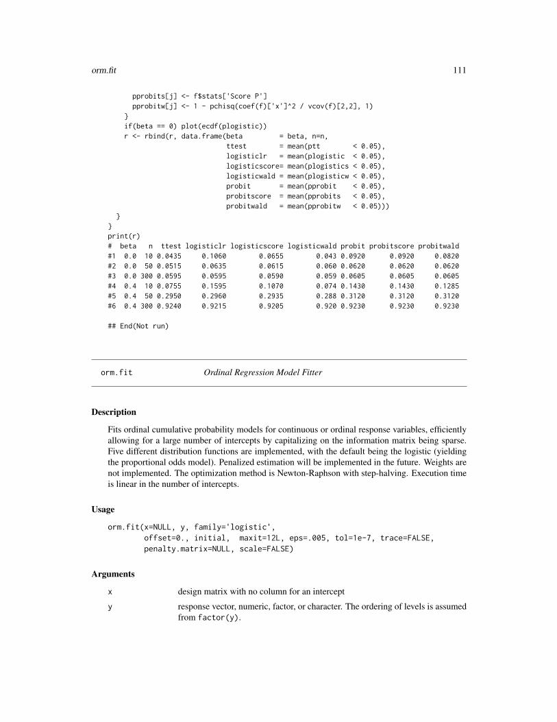
orm.fit 111
pprobits[j] <- f$stats['Score P']pprobitw[j] <- 1 - pchisq(coef(f)['x']^2 / vcov(f)[2,2], 1)
}if(beta == 0) plot(ecdf(plogistic))r <- rbind(r, data.frame(beta = beta, n=n,
ttest = mean(ptt < 0.05),logisticlr = mean(plogistic < 0.05),logisticscore= mean(plogistics < 0.05),logisticwald = mean(plogisticw < 0.05),probit = mean(pprobit < 0.05),probitscore = mean(pprobits < 0.05),probitwald = mean(pprobitw < 0.05)))
}}print(r)# beta n ttest logisticlr logisticscore logisticwald probit probitscore probitwald#1 0.0 10 0.0435 0.1060 0.0655 0.043 0.0920 0.0920 0.0820#2 0.0 50 0.0515 0.0635 0.0615 0.060 0.0620 0.0620 0.0620#3 0.0 300 0.0595 0.0595 0.0590 0.059 0.0605 0.0605 0.0605#4 0.4 10 0.0755 0.1595 0.1070 0.074 0.1430 0.1430 0.1285#5 0.4 50 0.2950 0.2960 0.2935 0.288 0.3120 0.3120 0.3120#6 0.4 300 0.9240 0.9215 0.9205 0.920 0.9230 0.9230 0.9230
## End(Not run)
orm.fit Ordinal Regression Model Fitter
Description
Fits ordinal cumulative probability models for continuous or ordinal response variables, efficientlyallowing for a large number of intercepts by capitalizing on the information matrix being sparse.Five different distribution functions are implemented, with the default being the logistic (yieldingthe proportional odds model). Penalized estimation will be implemented in the future. Weights arenot implemented. The optimization method is Newton-Raphson with step-halving. Execution timeis linear in the number of intercepts.
Usage
orm.fit(x=NULL, y, family='logistic',offset=0., initial, maxit=12L, eps=.005, tol=1e-7, trace=FALSE,penalty.matrix=NULL, scale=FALSE)
Arguments
x design matrix with no column for an intercept
y response vector, numeric, factor, or character. The ordering of levels is assumedfrom factor(y).

112 orm.fit
family the distribution family, corresponding to logistic (the default), Gaussian, Cauchy,Gumbel maximum (exp(−exp(−x)); extreme value type I), and Gumbel min-imum (1 − exp(−exp(x))) distributions. These are the cumulative distributionfunctions assumed for Prob[Y ≥ y|X]. The family argument can be an un-quoted or a quoted string, e.g. family=loglog or family="loglog". To usea built-in family, the string must be one of the following corresponding to theprevious list: logistic, probit, loglog,cloglog, cauchit. The user canalso provide her own customized family by setting family to a list with elementscumprob,inverse, deriv, deriv2; see the body of orm.fit for examples.An additional element, name must be given, which is a character string used toname the family for print and latex.
offset optional numeric vector containing an offset on the logit scale
initial vector of initial parameter estimates, beginning with the intercepts. If initialis not specified, the function computes the overall score χ2 test for the globalnull hypothesis of no regression.
maxit maximum no. iterations (default=12).
eps difference in −2log likelihood for declaring convergence. Default is .005. Ifthe −2log likelihood gets worse by eps/10 while the maximum absolute firstderivative of
-2 log
likelihood is below 1E-9, convergence is still declared. This handles the casewhere the initial estimates are MLEs, to prevent endless step-halving.
tol Singularity criterion. Default is 1e-7
trace set to TRUE to print -2 log likelihood, step-halving fraction, change in -2 loglikelihood, and maximum absolute value of first derivative at each iteration.
penalty.matrix a self-contained ready-to-use penalty matrix - seelrm
scale set to TRUE to subtract column means and divide by column standard deviationsof x before fitting, and to back-solve for the un-normalized covariance matrixand regression coefficients. This can sometimes make the model converge forvery large sample sizes where for example spline or polynomial component vari-ables create scaling problems leading to loss of precision when accumulatingsums of squares and crossproducts.
Value
a list with the following components:
call calling expression
freq table of frequencies for y in order of increasing y
yunique vector of sorted unique values of y
stats vector with the following elements: number of observations used in the fit, num-ber of unique y values, median y from among the observations used in the fit,maximum absolute value of first derivative of log likelihood, model likelihoodratio chi-square, d.f., P-value, score chi-square and its P-value, Spearman’s ρ

orm.fit 113
rank correlation between linear predictor and y, the Nagelkerke R2 index, theg-index, gr (the g-index on the ratio scale), and pdm (the mean absolute differ-ence between 0.5 and the estimated probability that y ≥ the marginal median).When penalty.matrix is present, the χ2, d.f., and P-value are not corrected forthe effective d.f.
fail set to TRUE if convergence failed (and maxit>1)
coefficients estimated parameters
var estimated variance-covariance matrix (inverse of information matrix). Note thatin the case of penalized estimation, var is not the improved sandwich-type esti-mator (which lrm does compute). The only intercept parameter included in thestored object is the middle intercept.
family, trans see orm
deviance -2 log likelihoods. When an offset variable is present, three deviances are com-puted: for intercept(s) only, for intercepts+offset, and for intercepts+offset+predictors.When there is no offset variable, the vector contains deviances for the intercept(s)-only model and the model with intercept(s) and predictors.
non.slopes number of intercepts in model
interceptRef the index of the middle (median) intercept used in computing the linear predictorand var
linear.predictors
the linear predictor using the first intercept
penalty.matrix see above
info.matrix see orm
Author(s)
Frank HarrellDepartment of Biostatistics, Vanderbilt [email protected]
See Also
orm, lrm, glm, gIndex, solve
Examples
#Fit an additive logistic model containing numeric predictors age,#blood.pressure, and sex, assumed to be already properly coded and#transformed## fit <- orm.fit(cbind(age,blood.pressure,sex), death)
114 pentrace
pentrace Trace AIC and BIC vs. Penalty
Description
For an ordinary unpenalized fit from lrm or ols and for a vector or list of penalties, fits a series oflogistic or linear models using penalized maximum likelihood estimation, and saves the effectivedegrees of freedom, Akaike Information Criterion (AIC), Schwarz Bayesian Information Criterion(BIC), and Hurvich and Tsai’s corrected AIC (AICc). Optionally pentrace can use the nlminbfunction to solve for the optimum penalty factor or combination of factors penalizing differentkinds of terms in the model. The effective.df function prints the original and effective degreesof freedom for a penalized fit or for an unpenalized fit and the best penalization determined froma previous invocation of pentrace if method="grid" (the default). The effective d.f. is computedseparately for each class of terms in the model (e.g., interaction, nonlinear). A plot method existsto plot the results, and a print method exists to print the most pertinent components. Both AICand BIC may be plotted if there is only one penalty factor type specified in penalty. Otherwise,the first two types of penalty factors are plotted, showing only the AIC.
Usage
pentrace(fit, penalty, penalty.matrix,method=c('grid','optimize'),which=c('aic.c','aic','bic'), target.df=NULL,fitter, pr=FALSE, tol=1e-7,keep.coef=FALSE, complex.more=TRUE, verbose=FALSE, maxit=12,subset, noaddzero=FALSE)
effective.df(fit, object)
## S3 method for class 'pentrace'print(x, ...)
## S3 method for class 'pentrace'plot(x, method=c('points','image'),
which=c('effective.df','aic','aic.c','bic'), pch=2, add=FALSE,ylim, ...)
Arguments
fit a result from lrm or ols with x=TRUE, y=TRUE and without using penalty orpenalty.matrix (or optionally using penalization in the case of effective.df)
penalty can be a vector or a list. If it is a vector, all types of terms in the model will be pe-nalized by the same amount, specified by elements in penalty, with a penaltyof zero automatically added. penalty can also be a list in the format docu-mented in the lrm function, except that elements of the list can be vectors. Theexpand.grid function is invoked by pentrace to generate all possible combina-tions of penalties. For example, specifying penalty=list(simple=1:2, nonlinear=1:3)
pentrace 115
will generate 6 combinations to try, so that the analyst can attempt to determinewhether penalizing more complex terms in the model more than the linear or cat-egorical variable terms will be beneficial. If complex.more=TRUE, it is assumedthat the variables given in penalty are listed in order from less complex to morecomplex. With method="optimize" penalty specifies an initial guess for thepenalty or penalties. If all term types are to be equally penalized, penaltyshould be a single number, otherwise it should be a list containing single num-bers as elements, e.g., penalty=list(simple=1, nonlinear=2). Experiencehas shown that the optimization algorithm is more likely to find a reasonablesolution when the starting value specified in penalty is too large rather than toosmall.
object an object returned by pentrace. For effective.df, object can be omitted ifthe fit was penalized.
penalty.matrix see lrm
method The default is method="grid" to print various indexes for all combinations ofpenalty parameters given by the user. Specify method="optimize" to havepentrace use nlminb to solve for the combination of penalty parameters thatgives the maximum value of the objective named in which, or, if target.dfis given, to find the combination that yields target.df effective total degreesof freedom for the model. When target.df is specified, method is set to"optimize" automatically. For plot.pentrace this parameter applies only ifmore than one penalty term-type was used. The default is to use open trian-gles whose sizes are proportional to the ranks of the AICs, plotting the first twopenalty factors respectively on the x and y axes. Use method="image" to plotan image plot.
which the objective to maximize for either method. Default is "aic.c" (correctedAIC). For plot.pentrace, which is a vector of names of criteria to show; de-fault is to plot all 4 types, with effective d.f. in its own separate plot
target.df applies only to method="optimize". See method. target.df makes sensemainly when a single type of penalty factor is specified.
fitter a fitting function. Default is lrm.fit (lm.pfit is always used for ols).
pr set to TRUE to print intermediate results
tol tolerance for declaring a matrix singular (see lrm.fit, solvet)
keep.coef set to TRUE to store matrix of regression coefficients for all the fits (correspond-ing to increasing values of penalty) in object Coefficients in the returnedlist. Rows correspond to penalties, columns to regression parameters.
complex.more By default if penalty is a list, combinations of penalties for which complexterms are penalized less than less complex terms will be dropped after expand.gridis invoked. Set complex.more=FALSE to allow more complex terms to be penal-ized less. Currently this option is ignored for method="optimize".
verbose set to TRUE to print number of intercepts and sum of effective degrees of freedom
maxit maximum number of iterations to allow in a model fit (default=12). This ispassed to the appropriate fitter function with the correct argument name. In-crease maxit if you had to when fitting the original unpenalized model.
116 pentrace
subset a logical or integer vector specifying rows of the design and response matricesto subset in fitting models. This is most useful for bootstrapping pentrace tosee if the best penalty can be estimated with little error so that variation due toselecting the optimal penalty can be safely ignored when bootstrapping standarderrors of regression coefficients and measures of predictive accuracy. See anexample below.
noaddzero set to TRUE to not add an unpenalized model to the list of models to fit
x a result from pentrace
pch used for method="points"
add set to TRUE to add to an existing plot. In that case, the effective d.f. plot is notre-drawn, but the AIC/BIC plot is added to.
ylim 2-vector of y-axis limits for plots other than effective d.f.
... other arguments passed to plot, lines, or image
Value
a list of class "pentrace" with elements penalty, df, objective, fit, var.adj, diag, results.all,and optionally Coefficients. The first 6 elements correspond to the fit that had the best objec-tive as named in the which argument, from the sequence of fits tried. Here fit is the fit objectfrom fitter which was a penalized fit, diag is the diagonal of the matrix used to compute theeffective d.f., and var.adj is Gray (1992) Equation 2.9, which is an improved covariance matrixfor the penalized beta. results.all is a data frame whose first few variables are the componentsof penalty and whose other columns are df, aic, bic, aic.c. results.all thus contains asummary of results for all fits attempted. When method="optimize", only two components arereturned: penalty and objective, and the object does not have a class.
Author(s)
Frank HarrellDepartment of BiostatisticsVanderbilt [email protected]
References
Gray RJ: Flexible methods for analyzing survival data using splines, with applications to breastcancer prognosis. JASA 87:942–951, 1992.
Hurvich CM, Tsai, CL: Regression and time series model selection in small samples. Biometrika76:297–307, 1989.
See Also
lrm, ols, solvet, rmsMisc, image
plot.Predict 117
Examples
n <- 1000 # define sample sizeset.seed(17) # so can reproduce the resultsage <- rnorm(n, 50, 10)blood.pressure <- rnorm(n, 120, 15)cholesterol <- rnorm(n, 200, 25)sex <- factor(sample(c('female','male'), n,TRUE))# Specify population model for log odds that Y=1L <- .4*(sex=='male') + .045*(age-50) +
(log(cholesterol - 10)-5.2)*(-2*(sex=='female') + 2*(sex=='male'))# Simulate binary y to have Prob(y=1) = 1/[1+exp(-L)]y <- ifelse(runif(n) < plogis(L), 1, 0)
f <- lrm(y ~ blood.pressure + sex * (age + rcs(cholesterol,4)),x=TRUE, y=TRUE)
p <- pentrace(f, seq(.2,1,by=.05))plot(p)p$diag # may learn something about fractional effective d.f.
# for each original parameterpentrace(f, list(simple=c(0,.2,.4), nonlinear=c(0,.2,.4,.8,1)))
# Bootstrap pentrace 5 times, making a plot of corrected AIC plot with 5 repsn <- nrow(f$x)plot(pentrace(f, seq(.2,1,by=.05)), which='aic.c',
col=1, ylim=c(30,120)) #original in blackfor(j in 1:5)
plot(pentrace(f, seq(.2,1,by=.05), subset=sample(n,n,TRUE)),which='aic.c', col=j+1, add=TRUE)
# Find penalty giving optimum corrected AIC. Initial guess is 1.0# Not implemented yet# pentrace(f, 1, method='optimize')
# Find penalty reducing total regression d.f. effectively to 5# pentrace(f, 1, target.df=5)
# Re-fit with penalty giving best aic.c without differential penalizationf <- update(f, penalty=p$penalty)effective.df(f)
plot.Predict Plot Effects of Variables Estimated by a Regression Model Fit
118 plot.Predict
Description
Uses lattice graphics to plot the effect of one or two predictors on the linear predictor or X betascale, or on some transformation of that scale. The first argument specifies the result of the Predictfunction. The predictor is always plotted in its original coding. plot.Predict uses the xYplotfunction unless formula is omitted and the x-axis variable is a factor, in which case it reverses thex- and y-axes and uses the Dotplot function.
If data is given, a rug plot is drawn showing the location/density of data values for the x-axis vari-able. If there is a groups (superposition) variable that generated separate curves, the data densityspecific to each class of points is shown. This assumes that the second variable was a factor variable.The rug plots are drawn by scat1d. When the same predictor is used on all x-axes, and multiplepanels are drawn, you can use subdata to specify an expression to subset according to other criteriain addition.
To plot effects instead of estimates (e.g., treatment differences as a function of interacting factors)see contrast.rms and summary.rms.
pantext creates a lattice panel function for including text such as that produced by print.anova.rmsinside a panel or in a base graphic.
Usage
## S3 method for class 'Predict'plot(x, formula, groups=NULL,
cond=NULL, varypred=FALSE, subset,xlim, ylim, xlab, ylab,data=NULL, subdata, anova=NULL, pval=FALSE, cex.anova=.85,col.fill=gray(seq(.825, .55, length=5)),adj.subtitle, cex.adj, cex.axis, perim=NULL, digits=4, nlevels=3,nlines=FALSE, addpanel, scat1d.opts=list(frac=0.025, lwd=0.3),type=NULL, yscale=NULL, scaletrans=function(z) z, ...)
pantext(object, x, y, cex=.5, adj=0, fontfamily="Courier", lattice=TRUE)
Arguments
x a data frame created by Predict, or for pantext the x-coordinate for text
formula the right hand side of a lattice formula reference variables in data frame x.You may not specify formula if you varied multiple predictors separately whencalling Predict. Otherwise, when formula is not given, plot.Predict con-structs one from information in x.
groups an optional name of one of the variables in x that is to be used as a grouping(superpositioning) variable. Note that groups does not contain the groups dataas is customary in lattice; it is only a single character string specifying thename of the grouping variable.
cond when plotting effects of different predictors, cond is a character string that spec-ifies a single variable name in x that can be used to form panels. Only applies ifusing rbind to combine several Predict results.

plot.Predict 119
varypred set to TRUE if x is the result of passing multiple Predict results, that representdifferent predictors, to rbind.Predict. This will cause the .set. variablecreated by rbind to be copied to the .predictor. variable.
subset a subsetting expression for restricting the rows of x that are used in plotting. Forexample, predictions may have been requested for males and females but onewants to plot only females.
xlim This parameter is seldom used, as limits are usually controlled with Predict.One reason to use xlim is to plot a factor variable on the x-axis that was cre-ated with the cut2 function with the levels.mean option, with val.lev=TRUEspecified to plot.Predict. In this case you may want the axis to have the rangeof the original variable values given to cut2 rather than the range of the meanswithin quantile groups.
ylim Range for plotting on response variable axis. Computed by default.
xlab Label for x-axis. Default is one given to asis, rcs, etc., which may have beenthe "label" attribute of the variable.
ylab Label for y-axis. If fun is not given, default is "log Odds" for lrm, "log Relative Hazard"for cph, name of the response variable for ols, TRUE or log(TRUE) for psm, or"X * Beta" otherwise.
data a data frame containing the original raw data on which the regression modelwere based, or at least containing the x-axis and grouping variable. If datais present and contains the needed variables, the original data are added to thegraph in the form of a rug plot using scat1d.
subdata if data is specified, an expression to be evaluated in the data environment thatevaluates to a logical vector specifying which observations in data to keep. Thiswill be intersected with the criterion for the groups variable. Example: if condi-tioning on two paneling variables using |a*b you can specify subdata=b==levels(b)[which.packet()[2]],where the 2 comes from the fact that b was listed second after the vertical bar(this assumes b is a factor in data. Another example: subdata=sex==c('male','female')[current.row()].
anova an object returned by anova.rms. If anova is specified, the overall test of asso-ciation for predictor plotted is added as text to each panel, located at the spot atwhich the panel is most empty unless there is significant empty space at the topor bottom of the panel; these areas are given preference.
pval specify pval=TRUE for anova to include not only the test statistic but also theP-value
cex.anova character size for the test statistic printed on the panel
col.fill a vector of colors used to fill confidence bands for successive superposed groups.Default is inceasingly dark gray scale.
adj.subtitle Set to FALSE to suppress subtitling the graph with the list of settings of non-graphed adjustment values.
cex.adj cex parameter for size of adjustment settings in subtitles. Default is 0.75 timespar("cex").
cex.axis cex parameter for x-axis tick labels
perim perim specifies a function having two arguments. The first is the vector of val-ues of the first variable that is about to be plotted on the x-axis. The second
120 plot.Predict
argument is the single value of the variable representing different curves, for thecurrent curve being plotted. The function’s returned value must be a logical vec-tor whose length is the same as that of the first argument, with values TRUE if thecorresponding point should be plotted for the current curve, FALSE otherwise.See one of the latter examples. If a predictor is not specified to plot, NULL ispassed as the second argument to perim, although it makes little sense to useperim when the same perim is used for multiple predictors.
digits Controls how numeric variables used for panel labels are formatted. The defaultis 4 significant digits.
nlevels when groups and formula are not specified, if any panel variable has nlevelsor fewer values, that variable is converted to a groups (superpositioning) vari-able. Set nlevels=0 to prevent this behavior. For other situations, a numericx-axis variable with nlevels or fewer unique values will cause a dot plot to bedrawn instead of an x-y plot.
nlines If formula is given, you can set nlines to TRUE to convert the x-axis variable toa factor and then to an integer. Points are plotted at integer values on the x-axisbut labeled with category levels. Points are connected by lines.
addpanel an additional panel function to call along with panel functions used for xYplotand Dotplot displays
scat1d.opts a list containing named elements that specifies parameters to scat1d when datais given. The col parameter is usually derived from other plotting informationand not specified by the user.
type a value ("l","p","b") to override default choices related to showing or con-necting points. Especially useful for discrete x coordinate variables.
yscale a lattice scale list for the y-axis to be added to what is automatically gener-ated for the x-axis. Example: yscale=list(at=c(.005,.01,.05),labels=format(c(.005,.01,.05))).See xyplot
scaletrans a function that operates on the scale object created by plot.Predict to pro-duce a modified scale object that is passed to the lattice graphics function. Thisis useful for adding other scales options or for changing the x-axis limits forone predictor.
... extra arguments to pass to xYplot or Dotplot. Some useful ones are label.curvesand abline. Set label.curves to FALSE to suppress labeling of separate curves.Default is TRUE, which causes labcurve to be invoked to place labels at posi-tions where the curves are most separated, labeling each curve with the fullcurve label. Set label.curves to a list to specify options to labcurve,e.g., label.curves= list(method="arrow",cex=.8). These option namesmay be abbreviated in the usual way arguments are abbreviated. Use for ex-ample label.curves=list(keys=letters[1:5]) to draw single lower caseletters on 5 curves where they are most separated, and automatically positiona legend in the most empty part of the plot. The col, lty, and lwd param-eters are passed automatically to labcurve although they may be overriddenhere. It is also useful to use . . . to pass lattice graphics parameters, e.g.par.settings=list(axis.text=list(cex=1.2), par.ylab.text=list(col='blue',cex=.9),par.xlab.text=list(cex=1)).
object an object having a print method

plot.Predict 121
y y-coordinate for placing text in a lattice panel or on a base graphics plot
cex character expansion size for pantext
adj text justification. Default is left justified.
fontfamily font family for pantext. Default is "Courier" which will line up columns of atable.
lattice set to FALSE to use text instead of ltext in the function generated by pantext,to use base graphics
Details
When a groups (superpositioning) variable was used, you can issue the command Key(...) afterprinting the result of plot.Predict, to draw a key for the groups.
Value
a lattice object ready to print for rendering.
Note
If plotting the effects of all predictors you can reorder the panels using for example p <- Predict(fit); p$.predictor. <-factor(p$.predictor., v)where v is a vector of predictor names specified in the desired order.
Author(s)
Frank HarrellDepartment of Biostatistics, Vanderbilt [email protected]
References
Fox J, Hong J (2009): Effect displays in R for multinomial and proportional-odds logit models:Extensions to the effects package. J Stat Software 32 No. 1.
See Also
Predict, ggplot.Predict, link{plotp.Predict}, rbind.Predict, datadist, predictrms, anova.rms,contrast.rms, summary.rms, rms, rmsMisc, labcurve, scat1d, xYplot, Overview
Examples
n <- 1000 # define sample sizeset.seed(17) # so can reproduce the resultsage <- rnorm(n, 50, 10)blood.pressure <- rnorm(n, 120, 15)cholesterol <- rnorm(n, 200, 25)sex <- factor(sample(c('female','male'), n,TRUE))label(age) <- 'Age' # label is in Hmisclabel(cholesterol) <- 'Total Cholesterol'label(blood.pressure) <- 'Systolic Blood Pressure'label(sex) <- 'Sex'
122 plot.Predict
units(cholesterol) <- 'mg/dl' # uses units.default in Hmiscunits(blood.pressure) <- 'mmHg'
# Specify population model for log odds that Y=1L <- .4*(sex=='male') + .045*(age-50) +
(log(cholesterol - 10)-5.2)*(-2*(sex=='female') + 2*(sex=='male'))# Simulate binary y to have Prob(y=1) = 1/[1+exp(-L)]y <- ifelse(runif(n) < plogis(L), 1, 0)
ddist <- datadist(age, blood.pressure, cholesterol, sex)options(datadist='ddist')
fit <- lrm(y ~ blood.pressure + sex * (age + rcs(cholesterol,4)),x=TRUE, y=TRUE)
an <- anova(fit)# Plot effects of all 4 predictors with test statistics from anova, and Pplot(Predict(fit), anova=an, pval=TRUE)plot(Predict(fit), data=llist(blood.pressure,age))
# rug plot for two of the predictors
p <- Predict(fit, name=c('age','cholesterol')) # Make 2 plotsplot(p)
p <- Predict(fit, age=seq(20,80,length=100), sex, conf.int=FALSE)# Plot relationship between age and log# odds, separate curve for each sex,
plot(p, subset=sex=='female' | age > 30)# No confidence interval, suppress estimates for males <= 30
p <- Predict(fit, age, sex)plot(p, label.curves=FALSE, data=llist(age,sex))
# use label.curves=list(keys=c('a','b'))'# to use 1-letter abbreviations# data= allows rug plots (1-dimensional scatterplots)# on each sex's curve, with sex-# specific density of age# If data were in data frame could have used that
p <- Predict(fit, age=seq(20,80,length=100), sex='male', fun=plogis)# works if datadist not used
plot(p, ylab=expression(hat(P)))# plot predicted probability in place of log odds
per <- function(x, y) x >= 30plot(p, perim=per) # suppress output for age < 30 but leave scale alone
# Take charge of the plot setup by specifying a lattice formulap <- Predict(fit, age, blood.pressure=c(120,140,160),
cholesterol=c(180,200,215), sex)plot(p, ~ age | blood.pressure*cholesterol, subset=sex=='male')# plot(p, ~ age | cholesterol*blood.pressure, subset=sex=='female')# plot(p, ~ blood.pressure|cholesterol*round(age,-1), subset=sex=='male')plot(p)
plot.Predict 123
# Plot the age effect as an odds ratio# comparing the age shown on the x-axis to age=30 years
ddist$limits$age[2] <- 30 # make 30 the reference value for age# Could also do: ddist$limits["Adjust to","age"] <- 30fit <- update(fit) # make new reference value take effectp <- Predict(fit, age, ref.zero=TRUE, fun=exp)plot(p, ylab='Age=x:Age=30 Odds Ratio',
abline=list(list(h=1, lty=2, col=2), list(v=30, lty=2, col=2)))
# Compute predictions for three predictors, with superpositioning or# conditioning on sex, combined into one graph
p1 <- Predict(fit, age, sex)p2 <- Predict(fit, cholesterol, sex)p3 <- Predict(fit, blood.pressure, sex)p <- rbind(age=p1, cholesterol=p2, blood.pressure=p3)plot(p, groups='sex', varypred=TRUE, adj.subtitle=FALSE)plot(p, cond='sex', varypred=TRUE, adj.subtitle=FALSE)
## Not run:# For males at the median blood pressure and cholesterol, plot 3 types# of confidence intervals for the probability on one plot, for varying ageages <- seq(20, 80, length=100)p1 <- Predict(fit, age=ages, sex='male', fun=plogis) # standard pointwisep2 <- Predict(fit, age=ages, sex='male', fun=plogis,
conf.type='simultaneous') # simultaneousp3 <- Predict(fit, age=c(60,65,70), sex='male', fun=plogis,
conf.type='simultaneous') # simultaneous 3 pts# The previous only adjusts for a multiplicity of 3 points instead of 100f <- update(fit, x=TRUE, y=TRUE)g <- bootcov(f, B=500, coef.reps=TRUE)p4 <- Predict(g, age=ages, sex='male', fun=plogis) # bootstrap percentilep <- rbind(Pointwise=p1, 'Simultaneous 100 ages'=p2,
'Simultaneous 3 ages'=p3, 'Bootstrap nonparametric'=p4)xYplot(Cbind(yhat, lower, upper) ~ age, groups=.set.,
data=p, type='l', method='bands', label.curve=list(keys='lines'))
## End(Not run)
# Plots for a parametric survival modeln <- 1000set.seed(731)age <- 50 + 12*rnorm(n)label(age) <- "Age"sex <- factor(sample(c('Male','Female'), n,
rep=TRUE, prob=c(.6, .4)))cens <- 15*runif(n)h <- .02*exp(.04*(age-50)+.8*(sex=='Female'))t <- -log(runif(n))/hlabel(t) <- 'Follow-up Time'e <- ifelse(t<=cens,1,0)t <- pmin(t, cens)
124 plot.Predict
units(t) <- "Year"ddist <- datadist(age, sex)Srv <- Surv(t,e)
# Fit log-normal survival model and plot median survival time vs. agef <- psm(Srv ~ rcs(age), dist='lognormal')med <- Quantile(f) # Creates function to compute quantiles
# (median by default)p <- Predict(f, age, fun=function(x) med(lp=x))plot(p, ylab="Median Survival Time")# Note: confidence intervals from this method are approximate since# they don't take into account estimation of scale parameter
# Fit an ols model to log(y) and plot the relationship between x1# and the predicted mean(y) on the original scale without assuming# normality of residuals; use the smearing estimator# See help file for rbind.Predict for a method of showing two# types of confidence intervals simultaneously.set.seed(1)x1 <- runif(300)x2 <- runif(300)ddist <- datadist(x1,x2)y <- exp(x1+x2-1+rnorm(300))f <- ols(log(y) ~ pol(x1,2)+x2)r <- resid(f)smean <- function(yhat)smearingEst(yhat, exp, res, statistic='mean')formals(smean) <- list(yhat=numeric(0), res=r[!is.na(r)])#smean$res <- r[!is.na(r)] # define default res argument to functionplot(Predict(f, x1, fun=smean), ylab='Predicted Mean on y-scale')
# Make an 'interaction plot', forcing the x-axis variable to be# plotted at integer values but labeled with category levelsn <- 100set.seed(1)gender <- c(rep('male', n), rep('female',n))m <- sample(c('a','b'), 2*n, TRUE)d <- datadist(gender, m); options(datadist='d')anxiety <- runif(2*n) + .2*(gender=='female') + .4*(gender=='female' & m=='b')tapply(anxiety, llist(gender,m), mean)f <- ols(anxiety ~ gender*m)p <- Predict(f, gender, m)plot(p) # horizontal dot chart; usually preferred for categorical predictorsKey(.5, .5)plot(p, ~gender, groups='m', nlines=TRUE)plot(p, ~m, groups='gender', nlines=TRUE)plot(p, ~gender|m, nlines=TRUE)
options(datadist=NULL)
## Not run:# Example in which separate curves are shown for 4 income values
plot.xmean.ordinaly 125
# For each curve the estimated percentage of voters voting for# the democratic party is plotted against the percent of voters# who graduated from college. Data are county-level percents.
incomes <- seq(22900, 32800, length=4)# equally spaced to outer quintilesp <- Predict(f, college, income=incomes, conf.int=FALSE)plot(p, xlim=c(0,35), ylim=c(30,55))
# Erase end portions of each curve where there are fewer than 10 counties having# percent of college graduates to the left of the x-coordinate being plotted,# for the subset of counties having median family income with 1650# of the target income for the curve
show.pts <- function(college.pts, income.pt) {s <- abs(income - income.pt) < 1650 #assumes income known to top framex <- college[s]x <- sort(x[!is.na(x)])n <- length(x)low <- x[10]; high <- x[n-9]college.pts >= low & college.pts <= high
}
plot(p, xlim=c(0,35), ylim=c(30,55), perim=show.pts)
# Rename variables for better plotting of a long list of predictorsf <- ...p <- Predict(f)re <- c(trt='treatment', diabet='diabetes', sbp='systolic blood pressure')
for(n in names(re)) {names(p)[names(p)==n] <- re[n]p$.predictor.[p$.predictor.==n] <- re[n]}
plot(p)
## End(Not run)
plot.xmean.ordinaly Plot Mean X vs. Ordinal Y
Description
Separately for each predictor variable X in a formula, plots the mean of X vs. levels of Y . Thenunder the proportional odds assumption, the expected value of the predictor for each Y value isalso plotted (as a dotted line). This plot is useful for assessing the ordinality assumption for Yseparately for each X , and for assessing the proportional odds assumption in a simple univariableway. If several predictors do not distinguish adjacent categories of Y , those levels may need to bepooled. This display assumes that each predictor is linearly related to the log odds of each event inthe proportional odds model. There is also an option to plot the expected means assuming a forwardcontinuation ratio model.

126 plot.xmean.ordinaly
Usage
## S3 method for class 'xmean.ordinaly'plot(x, data, subset, na.action, subn=TRUE,
cr=FALSE, topcats=1, cex.points=.75, ...)
Arguments
x an S formula. Response variable is treated as ordinal. For categorical predictors,a binary version of the variable is substituted, specifying whether or not thevariable equals the modal category. Interactions or non-linear effects are notallowed.
data a data frame or frame number
subset vector of subscripts or logical vector describing subset of data to analyze
na.action defaults to na.keep so all NAs are initially retained. Then NAs are deleted onlyfor each predictor currently being plotted. Specify na.action=na.delete toremove observations that are missing on any of the predictors (or the response).
subn set to FALSE to suppress a left bottom subtitle specifying the sample size used inconstructing each plot
cr set to TRUE to plot expected values by levels of the response, assuming a forwardcontinuation ratio model holds. The function is fairly slow when this option isspecified.
topcats When a predictor is categorical, by default only the proportion of observationsin the overall most frequent category will be plotted against response variablestrata. Specify a higher value of topcats to make separate plots for the propor-tion in the k most frequent predictor categories, where k is min(ncat-1, topcats)and ncat is the number of unique values of the predictor.
cex.points if cr is TRUE, specifies the size of the "C" that is plotted. Default is 0.75.
... other arguments passed to plot and lines
Side Effects
plots
Author(s)
Frank HarrellDepartment of BiostatisticsVanderbilt [email protected]
References
Harrell FE et al. (1998): Development of a clinical prediction model for an ordinal outcome. Statin Med 17:909–44.
plotp.Predict 127
See Also
lrm, residuals.lrm, cr.setup, summary.formula, biVar.
Examples
# Simulate data from a population proportional odds modelset.seed(1)n <- 400age <- rnorm(n, 50, 10)blood.pressure <- rnorm(n, 120, 15)region <- factor(sample(c('north','south','east','west'), n, replace=TRUE))L <- .2*(age-50) + .1*(blood.pressure-120)p12 <- plogis(L) # Pr(Y>=1)p2 <- plogis(L-1) # Pr(Y=2)p <- cbind(1-p12, p12-p2, p2) # individual class probabilites# Cumulative probabilities:cp <- matrix(cumsum(t(p)) - rep(0:(n-1), rep(3,n)), byrow=TRUE, ncol=3)y <- (cp < runif(n)) %*% rep(1,3)# Thanks to Dave Krantz <[email protected]> for this trick
par(mfrow=c(2,2))plot.xmean.ordinaly(y ~ age + blood.pressure + region, cr=TRUE, topcats=2)par(mfrow=c(1,1))# Note that for unimportant predictors we don't care very much about the# shapes of these plots. Use the Hmisc chiSquare function to compute# Pearson chi-square statistics to rank the variables by unadjusted# importance without assuming any ordering of the response:chiSquare(y ~ age + blood.pressure + region, g=3)chiSquare(y ~ age + blood.pressure + region, g=5)
plotp.Predict Plot Effects of Variables Estimated by a Regression Model Fit Usingplotly
Description
Uses plotly graphics (without using ggplot2) to plot the effect of one or two predictors on thelinear predictor or X beta scale, or on some transformation of that scale. The first argument specifiesthe result of the Predict function. The predictor is always plotted in its original coding. Hovertext shows point estimates, confidence intervals, and on the leftmost x-point, adjustment variablesettings.
If Predict was run with no variable settings, so that each predictor is varied one at a time, theresult of plotp.Predict is a list with two elements. The first, named Continuous, is a plotlyobject containing a single graphic with all the continuous predictors varying. The second, namedCategorical, is a plotly object containing a single graphic with all the categorical predictorsvarying. If there are no categorical predictors, the value returned by by plotp.Predict is a singleplotly object and not a list of objects.
128 plotp.Predict
If rdata is given, a spike histogram is drawn showing the location/density of data values for thex-axis variable. If there is a superposition variable that generated separate curves, the data densityspecific to each class of points is shown. The histograms are drawn by histSpikeg.
To plot effects instead of estimates (e.g., treatment differences as a function of interacting factors)see contrast.rms and summary.rms.
Unlike ggplot.Predict, plotp.Predict does not handle groups, anova, or perim arguments.
Usage
## S3 method for class 'Predict'plotp(data, subset, xlim, ylim, xlab, ylab,
rdata=NULL, nlevels=3, vnames=c('labels','names'),histSpike.opts=list(frac=function(f) 0.01 +
0.02 * sqrt(f - 1)/sqrt(max(f, 2) - 1), side=1, nint=100),ncols=3, width=800, ...)
plotp(data, ...)
Arguments
data a data frame created by Predict
subset a subsetting expression for restricting the rows of data that are used in plotting.For example, predictions may have been requested for males and females butone wants to plot only females.
xlim ignored unless predictors were specified to Predict. Specifies the x-axis limitsof the single plot produced.
ylim Range for plotting on response variable axis. Computed by default and includesthe confidence limits.
xlab Label for x-axis when a single plot is made, i.e., when a predictor is specifiedto Predict. Default is one given to asis, rcs, etc., which may have been the"label" attribute of the variable.
ylab Label for y-axis. If fun is not given, default is "log Odds" for lrm, "log Relative Hazard"for cph, name of the response variable for ols, TRUE or log(TRUE) for psm, or"X * Beta" otherwise. Specify ylab=NULL to omit y-axis labels.
rdata a data frame containing the original raw data on which the regression modelwere based, or at least containing the x-axis and grouping variable. If rdatais present and contains the needed variables, the original data are added to thegraph in the form of a spike histogram using histSpikeg in the Hmisc package.
nlevels A non-numeric x-axis variable with nlevels or fewer unique values will causea horizontal dot plot to be drawn instead of an x-y plot.
vnames applies to the case where multiple plots are produced separately by predictor.Set to 'names' to use variable names instead of labels for these small plots.
histSpike.opts a list containing named elements that specifies parameters to histSpikeg whenrdata is given. The col parameter is usually derived from other plotting infor-mation and not specified by the user.

plotp.Predict 129
ncols number of columns of plots to use when plotting multiple continuous predictors
width width in pixels for plotly graphics
... ignored
Value
a plotly object or a list containing two elements, each one a plotly object
Author(s)
Frank HarrellDepartment of Biostatistics, Vanderbilt [email protected]
References
Fox J, Hong J (2009): Effect displays in R for multinomial and proportional-odds logit models:Extensions to the effects package. J Stat Software 32 No. 1.
See Also
Predict, rbind.Predict, datadist, predictrms, contrast.rms, summary.rms, rms, rmsMisc,plot.Predict, ggplot.Predict, histSpikeg, Overview
Examples
## Not run:n <- 350 # define sample sizeset.seed(17) # so can reproduce the resultsage <- rnorm(n, 50, 10)blood.pressure <- rnorm(n, 120, 15)cholesterol <- rnorm(n, 200, 25)sex <- factor(sample(c('female','male'), n,TRUE))label(age) <- 'Age' # label is in Hmisclabel(cholesterol) <- 'Total Cholesterol'label(blood.pressure) <- 'Systolic Blood Pressure'label(sex) <- 'Sex'units(cholesterol) <- 'mg/dl' # uses units.default in Hmiscunits(blood.pressure) <- 'mmHg'
# Specify population model for log odds that Y=1L <- .4*(sex=='male') + .045*(age-50) +
(log(cholesterol - 10)-5.2)*(-2*(sex=='female') + 2*(sex=='male')) +.01 * (blood.pressure - 120)
# Simulate binary y to have Prob(y=1) = 1/[1+exp(-L)]y <- ifelse(runif(n) < plogis(L), 1, 0)
ddist <- datadist(age, blood.pressure, cholesterol, sex)options(datadist='ddist')
fit <- lrm(y ~ blood.pressure + sex * (age + rcs(cholesterol,4)),
130 pphsm
x=TRUE, y=TRUE)
p <- plotp(Predict(fit))p$Continuousp$Categorical# When using Rmarkdown html notebook, best to use# prList(p) to render the two objectsplotp(Predict(fit), rdata=llist(blood.pressure, age))$Continuous# spike histogram plot for two of the predictors
p <- Predict(fit, name=c('age','cholesterol')) # Make 2 plotsplotp(p)
p <- Predict(fit, age, sex)plotp(p, rdata=llist(age,sex))# rdata= allows rug plots (1-dimensional scatterplots)# on each sex's curve, with sex-# specific density of age# If data were in data frame could have used thatp <- Predict(fit, age=seq(20,80,length=100), sex='male', fun=plogis)# works if datadist not usedplotp(p, ylab='P')# plot predicted probability in place of log odds
# Compute predictions for three predictors, with superpositioning or# conditioning on sex, combined into one graph
p1 <- Predict(fit, age, sex)p2 <- Predict(fit, cholesterol, sex)p3 <- Predict(fit, blood.pressure, sex)p <- rbind(age=p1, cholesterol=p2, blood.pressure=p3)plotp(p, ncols=2, rdata=llist(age, cholesterol, sex))
## End(Not run)
pphsm Parametric Proportional Hazards form of AFT Models
Description
Translates an accelerated failure time (AFT) model fitted by psm to proportional hazards form, ifthe fitted model was a Weibull or exponential model (extreme value distribution with "log" link).
Usage
pphsm(fit)## S3 method for class 'pphsm'print(x, digits=max(options()$digits - 4, 3),correlation=TRUE, ...)## S3 method for class 'pphsm'vcov(object, ...)
predab.resample 131
Arguments
fit fit object created by psm
x result of psm
digits how many significant digits are to be used for the returned value
correlation set to FALSE to suppress printing of correlation matrix of parameter estimates
... ignored
object a pphsm object
Value
a new fit object with transformed parameter estimates
Author(s)
Frank HarrellDepartment of BiostatisticsVanderbilt [email protected]
See Also
psm, summary.rms, print.pphsm
Examples
set.seed(1)S <- Surv(runif(100))x <- runif(100)dd <- datadist(x); options(datadist='dd')f <- psm(S ~ x, dist="exponential")summary(f) # effects on log(T) scalef.ph <- pphsm(f)## Not run: summary(f.ph) # effects on hazard ratio scaleoptions(datadist=NULL)
predab.resample Predictive Ability using Resampling
Description
predab.resample is a general-purpose function that is used by functions for specific models. Itcomputes estimates of optimism of, and bias-corrected estimates of a vector of indexes of predictiveaccuracy, for a model with a specified design matrix, with or without fast backward step-down ofpredictors. If bw=TRUE, the design matrix x must have been created by ols, lrm, or cph. If bw=TRUE,predab.resample stores as the kept attribute a logical matrix encoding which factors were selectedat each repetition.

132 predab.resample
Usage
predab.resample(fit.orig, fit, measure,method=c("boot","crossvalidation",".632","randomization"),bw=FALSE, B=50, pr=FALSE, prmodsel=TRUE,rule="aic", type="residual", sls=.05, aics=0,tol=1e-12, force=NULL, estimates=TRUE,non.slopes.in.x=TRUE, kint=1,cluster, subset, group=NULL,allow.varying.intercepts=FALSE, debug=FALSE, ...)
Arguments
fit.orig object containing the original full-sample fit, with the x=TRUE and y=TRUE op-tions specified to the model fitting function. This model should be the FULLmodel including all candidate variables ever excluded because of poor associa-tions with the response.
fit a function to fit the model, either the original model fit, or a fit in a sample. fit hasas arguments x,y, iter, penalty, penalty.matrix, xcol, and other argumentspassed to predab.resample. If you don’t want iter as an argument inside thedefinition of fit, add . . . to the end of its argument list. iter is passed to fitto inform the function of the sampling repetition number (0=original sample).If bw=TRUE, fit should allow for the possibility of selecting no predictors, i.e.,it should fit an intercept-only model if the model has intercept(s). fit mustreturn objects coef and fail (fail=TRUE if fit failed due to singularity ornon-convergence - these cases are excluded from summary statistics). fit mustadd design attributes to the returned object if bw=TRUE. The penalty.matrixparameter is not used if penalty=0. The xcol vector is a vector of columns ofX to be used in the current model fit. For ols and psm it includes a 1 for theintercept position. xcol is not defined if iter=0 unless the initial fit had beenfrom a backward step-down. xcol is used to select the correct rows and columnsof penalty.matrix for the current variables selected, for example.
measure a function to compute a vector of indexes of predictive accuracy for a givenfit. For method=".632" or method="crossval", it will make the most sensefor measure to compute only indexes that are independent of sample size. Themeasure function should take the following arguments or use . . . : xbeta (Xbeta for current fit), y, evalfit, fit, iter, and fit.orig. iter is as in fit.evalfit is set to TRUE by predab.resample if the fit is being evaluated onthe sample used to make the fit, FALSE otherwise; fit.orig is the fit objectreturned by the original fit on the whole sample. Using evalfit will sometimessave computations. For example, in bootstrapping the area under an ROC curvefor a logistic regression model, lrm already computes the area if the fit is on thetraining sample. fit.orig is used to pass computed configuration parametersfrom the original fit such as quantiles of predicted probabilities that are used ascut points in other samples. The vector created by measure should have names()associated with it.
method The default is "boot" for ordinary bootstrapping (Efron, 1983, Eq. 2.10). Use".632" for Efron’s .632 method (Efron, 1983, Section 6 and Eq. 6.10), "crossvalidation"

predab.resample 133
for grouped cross–validation, "randomization" for the randomization method.May be abbreviated down to any level, e.g. "b", ".", "cross", "rand".
bw Set to TRUE to do fast backward step-down for each training sample. Default isFALSE.
B Number of repetitions, default=50. For method="crossvalidation", this isalso the number of groups the original sample is split into.
pr TRUE to print results for each sample. Default is FALSE.prmodsel set to FALSE to suppress printing of model selection output such as that from
fastbw.rule Stopping rule for fastbw, "aic" or "p". Default is "aic" to use Akaike’s infor-
mation criterion.type Type of statistic to use in stopping rule for fastbw, "residual" (the default) or
"individual".sls Significance level for stopping in fastbw if rule="p". Default is .05.aics Stopping criteria for rule="aic". Stops deleting factors when chi-square - 2
times d.f. falls below aics. Default is 0.tol Tolerance for singularity checking. Is passed to fit and fastbw.force see fastbw
estimates see print.fastbwnon.slopes.in.x
set to FALSE if the design matrix x does not have columns for intercepts andthese columns are needed
kint For multiple intercept models such as the ordinal logistic model, you may spec-ify which intercept to use as kint. This affects the linear predictor that is passedto measure.
cluster Vector containing cluster identifiers. This can be specified only if method="boot".If it is present, the bootstrap is done using sampling with replacement from theclusters rather than from the original records. If this vector is not the same lengthas the number of rows in the data matrix used in the fit, an attempt will be madeto use naresid on fit.orig to conform cluster to the data. See bootcov formore about this.
subset specify a vector of positive or negative integers or a logical vector when youwant to have the measure function compute measures of accuracy on a subsetof the data. The whole dataset is still used for all model development. Forexample, you may want to validate or calibrate a model by assessing thepredictions on females when the fit was based on males and females. Whenyou use cr.setup to build extra observations for fitting the continuation ratioordinal logistic model, you can use subset to specify which cohort or obser-vations to use for deriving indexes of predictive accuracy. For example, specifysubset=cohort=="all" to validate the model for the first layer of the continu-ation ratio model (Prob(Y=0)).
group a grouping variable used to stratify the sample upon bootstrapping. This allowsone to handle k-sample problems, i.e., each bootstrap sample will be forcedto selected the same number of observations from each level of group as thenumber appearing in the original dataset.
134 predab.resample
allow.varying.intercepts
set to TRUE to not throw an error if the number of intercepts varies from fit to fitdebug set to TRUE to print subscripts of all training and test samples... The user may add other arguments here that are passed to fit and measure.
Details
For method=".632", the program stops with an error if every observation is not omitted at least oncefrom a bootstrap sample. Efron’s ".632" method was developed for measures that are formulatedin terms on per-observation contributions. In general, error measures (e.g., ROC areas) cannot bewritten in this way, so this function uses a heuristic extension to Efron’s formulation in which it isassumed that the average error measure omitting the ith observation is the same as the average errormeasure omitting any other observation. Then weights are derived for each bootstrap repetition andweighted averages over the B repetitions can easily be computed.
Value
a matrix of class "validate" with rows corresponding to indexes computed by measure, and thefollowing columns:
index.orig indexes in original overall fittraining average indexes in training samplestest average indexes in test samplesoptimism average training-test except for method=".632" - is .632 times (index.orig - test)index.corrected
index.orig-optimism
n number of successful repetitions with the given index non-missing
. Also contains an attribute keepinfo if measure returned such an attribute when run on the originalfit.
Author(s)
Frank HarrellDepartment of Biostatistics, Vanderbilt [email protected]
References
Efron B, Tibshirani R (1997). Improvements on cross-validation: The .632+ bootstrap method.JASA 92:548–560.
See Also
rms, validate, fastbw, lrm, ols, cph, bootcov, setPb
Examples
# See the code for validate.ols for an example of the use of# predab.resample

Predict 135
Predict Compute Predicted Values and Confidence Limits
Description
Predict allows the user to easily specify which predictors are to vary. When the vector of valuesover which a predictor should vary is not specified, the range will be all levels of a categorical pre-dictor or equally-spaced points between the datadist "Low:prediction" and "High:prediction"values for the variable (datadist by default uses the 10th smallest and 10th largest predictor valuesin the dataset). Predicted values are the linear predictor (X beta), a user-specified transformationof that scale, or estimated probability of surviving past a fixed single time point given the linearpredictor. Predict is usually used for plotting predicted values but there is also a print method.
When the first argument to Predict is a fit object created by bootcov with coef.reps=TRUE, con-fidence limits come from the stored matrix of bootstrap repetitions of coefficients, using bootstrappercentile nonparametric confidence limits, basic bootstrap, or BCa limits. Such confidence inter-vals do not make distributional assumptions. You can force Predict to instead use the bootstrapcovariance matrix by setting usebootcoef=FALSE. If coef.reps was FALSE, usebootcoef=FALSEis the default.
There are ggplot, plotp, and plot methods for Predict objects that makes it easy to show pre-dicted values and confidence bands.
The rbind method for Predict objects allows you to create separate sets of predictions under dif-ferent situations and to combine them into one set for feeding to plot.Predict, ggplot.Predict,or plotp.Predict. For example you might want to plot confidence intervals for means and forindividuals using ols, and have the two types of confidence bands be superposed onto one plot orplaced into two panels. Another use for rbind is to combine predictions from quantile regressionmodels that predicted three different quantiles.
If conf.type="simultaneous", simultaneous (over all requested predictions) confidence limitsare computed. See the predictrms function for details.
Usage
Predict(x, ..., fun,type = c("predictions", "model.frame", "x"),np = 200, conf.int = 0.95,conf.type = c("mean", "individual","simultaneous"),usebootcoef=TRUE, boot.type=c("percentile","bca","basic"),adj.zero = FALSE, ref.zero = FALSE,kint=NULL, time = NULL, loglog = FALSE, digits=4, name,factors=NULL, offset=NULL)
## S3 method for class 'Predict'print(x, ...)
## S3 method for class 'Predict'rbind(..., rename)
136 Predict
Arguments
x an rms fit object, or for print the result of Predict. options(datadist="d")must have been specified (where d was created by datadist), or it must havebeen in effect when the the model was fitted.
... One or more variables to vary, or single-valued adjustment values. Specify avariable name without an equal sign to use the default display range, or anyrange you choose (e.g. seq(0,100,by=2),c(2,3,7,14)). The default list ofvalues for which predictions are made is taken as the list of unique values ofthe variable if they number fewer than 11. For variables with > 10 uniquevalues, np equally spaced values in the range are used for plotting if the rangeis not specified. Variables not specified are set to the default adjustment valuelimits[2], i.e. the median for continuous variables and a reference category fornon-continuous ones. Later variables define adjustment settings. For categoricalvariables, specify the class labels in quotes when specifying variable values. Ifthe levels of a categorical variable are numeric, you may omit the quotes. Forvariables not described using datadist, you must specify explicit ranges andadjustment settings for predictors that were in the model. If no variables arespecified in . . . , predictions will be made by separately varying all predictors inthe model over their default range, holding the other predictors at their adjust-ment values. This has the same effect as specifying name as a vector containingall the predictors. For rbind, . . . represents a series of results from Predict. Ifyou name the results, these names will be taken as the values of the new .set.variable added to the concatenated data frames. See an example below.
fun an optional transformation of the linear predictor. Specify fun='mean' if thefit is a proportional odds model fit and you ran bootcov with coef.reps=TRUE.This will let the mean function be re-estimated for each bootstrap rep to properlyaccount for all sources of uncertainty in estimating the mean response.
type defaults to providing predictions. Set to "model.frame" to return a data frameof predictor settings used. Set to "x" to return the corresponding design matrixconstructed from the predictor settings.
np the number of equally-spaced points computed for continuous predictors thatvary, i.e., when the specified value is . or NA
conf.int confidence level. Default is 0.95. Specify FALSE to suppress.
conf.type type of confidence interval. Default is "mean" which applies to all models. Formodels containing a residual variance (e.g, ols), you can specify conf.type="individual"instead, to obtain limits on the predicted value for an individual subject. Spec-ify conf.type="simultaneous" to obtain simultaneous confidence bands formean predictions with family-wise coverage of conf.int.
usebootcoef set to FALSE to force the use of the bootstrap covariance matrix estimator evenwhen bootstrap coefficient reps are present
boot.type set to 'bca' to compute BCa confidence limits or 'basic' to use the basicbootstrap. The default is to compute percentile intervals
adj.zero Set to TRUE to adjust all non-plotted variables to 0 (or reference cell for categor-ical variables) and to omit intercept(s) from consideration. Default is FALSE.
Predict 137
ref.zero Set to TRUE to subtract a constant from Xβ before plotting so that the refer-ence value of the x-variable yields y=0. This is done before applying functionfun. This is especially useful for Cox models to make the hazard ratio be 1.0 atreference values, and the confidence interval have width zero.
kint This is only useful in a multiple intercept model such as the ordinal logisticmodel. There to use to second of three intercepts, for example, specify kint=2.The default is 1 for lrm and the middle intercept corresponding to the median yfor orm.
time Specify a single time u to cause function survest to be invoked to plot theprobability of surviving until time u when the fit is from cph or psm.
loglog Specify loglog=TRUE to plot log[-log(survival)] instead of survival, whentime is given.
digits Controls how “adjust-to” values are plotted. The default is 4 significant digits.name Instead of specifying the variables to vary in the variables (. . . ) list, you can
specify one or more variables by specifying a vector of character string variablenames in the name argument. Using this mode you cannot specify a list of vari-able values to use; prediction is done as if you had said e.g. age without theequal sign. Also, interacting factors can only be set to their reference valuesusing this notation.
factors an alternate way of specifying . . . , mainly for use by survplot or gendata.This must be a list with one or more values for each variable listed, with NAvalues for default ranges.
offset a list containing one value for one variable, which is mandatory if the modelincluded an offset term. The variable name must match the innermost variablename in the offset term. The single offset is added to all predicted values.
rename If you are concatenating predictor sets using rbind and one or more of the vari-ables were renamed for one or more of the sets, but these new names representdifferent versions of the same predictors (e.g., using or not using imputation),you can specify a named character vector to rename predictors to a central name.For example, specify rename=c(age.imputed='age', corrected.bp='bp')to rename from old names age.imputed, corrected.bp to age, bp. Thishappens before concatenation of rows.
Details
When there are no intercepts in the fitted model, plot subtracts adjustment values from each factorwhile computing variances for confidence limits.
Specifying time will not work for Cox models with time-dependent covariables. Use survest orsurvfit for that purpose.
Value
a data frame containing all model predictors and the computed values yhat, lower, upper, the lattertwo if confidence intervals were requested. The data frame has an additional class "Predict". Ifname is specified or no predictors are specified in . . . , the resulting data frame has an additionalvariable called .predictor. specifying which predictor is currently being varied. .predictor. ishandy for use as a paneling variable in lattice or ggplot2 graphics.

138 Predict
Author(s)
Frank HarrellDepartment of Biostatistics, Vanderbilt [email protected]
See Also
plot.Predict, ggplot.Predict, plotp.Predict, datadist, predictrms, contrast.rms, summary.rms,rms, rms.trans, survest, survplot, rmsMisc, transace, rbind, bootcov, bootBCa, boot.ci
Examples
n <- 1000 # define sample sizeset.seed(17) # so can reproduce the resultsage <- rnorm(n, 50, 10)blood.pressure <- rnorm(n, 120, 15)cholesterol <- rnorm(n, 200, 25)sex <- factor(sample(c('female','male'), n,TRUE))label(age) <- 'Age' # label is in Hmisclabel(cholesterol) <- 'Total Cholesterol'label(blood.pressure) <- 'Systolic Blood Pressure'label(sex) <- 'Sex'units(cholesterol) <- 'mg/dl' # uses units.default in Hmiscunits(blood.pressure) <- 'mmHg'
# Specify population model for log odds that Y=1L <- .4*(sex=='male') + .045*(age-50) +
(log(cholesterol - 10)-5.2)*(-2*(sex=='female') + 2*(sex=='male'))# Simulate binary y to have Prob(y=1) = 1/[1+exp(-L)]y <- ifelse(runif(n) < plogis(L), 1, 0)
ddist <- datadist(age, blood.pressure, cholesterol, sex)options(datadist='ddist')
fit <- lrm(y ~ blood.pressure + sex * (age + rcs(cholesterol,4)))Predict(fit, age, cholesterol, np=4)Predict(fit, age=seq(20,80,by=10), sex, conf.int=FALSE)Predict(fit, age=seq(20,80,by=10), sex='male') # works if datadist not used# Get simultaneous confidence limits accounting for making 7 estimates# Predict(fit, age=seq(20,80,by=10), sex='male', conf.type='simult')# (this needs the multcomp package)
ddist$limits$age[2] <- 30 # make 30 the reference value for age# Could also do: ddist$limits["Adjust to","age"] <- 30fit <- update(fit) # make new reference value take effectPredict(fit, age, ref.zero=TRUE, fun=exp)
# Make two curves, and plot the predicted curves as two trellis panelsw <- Predict(fit, age, sex)require(lattice)xyplot(yhat ~ age | sex, data=w, type='l')# To add confidence bands we need to use the Hmisc xYplot function in
Predict 139
# place of xyplotxYplot(Cbind(yhat,lower,upper) ~ age | sex, data=w,
method='filled bands', type='l', col.fill=gray(.95))# If non-displayed variables were in the model, add a subtitle to show# their settings using title(sub=paste('Adjusted to',attr(w,'info')$adjust),adj=0)# Easier: feed w into plot.Predict, ggplot.Predict, plotp.Predict## Not run:# Predictions form a parametric survival modeln <- 1000set.seed(731)age <- 50 + 12*rnorm(n)label(age) <- "Age"sex <- factor(sample(c('Male','Female'), n,
rep=TRUE, prob=c(.6, .4)))cens <- 15*runif(n)h <- .02*exp(.04*(age-50)+.8*(sex=='Female'))t <- -log(runif(n))/hlabel(t) <- 'Follow-up Time'e <- ifelse(t<=cens,1,0)t <- pmin(t, cens)units(t) <- "Year"ddist <- datadist(age, sex)Srv <- Surv(t,e)
# Fit log-normal survival model and plot median survival time vs. agef <- psm(Srv ~ rcs(age), dist='lognormal')med <- Quantile(f) # Creates function to compute quantiles
# (median by default)Predict(f, age, fun=function(x)med(lp=x))# Note: This works because med() expects the linear predictor (X*beta)# as an argument. Would not work if use# ref.zero=TRUE or adj.zero=TRUE.# Also, confidence intervals from this method are approximate since# they don't take into account estimation of scale parameter
# Fit an ols model to log(y) and plot the relationship between x1# and the predicted mean(y) on the original scale without assuming# normality of residuals; use the smearing estimator. Before doing# that, show confidence intervals for mean and individual log(y),# and for the latter, also show bootstrap percentile nonparametric# pointwise confidence limitsset.seed(1)x1 <- runif(300)x2 <- runif(300)ddist <- datadist(x1,x2); options(datadist='ddist')y <- exp(x1+ x2 - 1 + rnorm(300))f <- ols(log(y) ~ pol(x1,2) + x2, x=TRUE, y=TRUE) # x y for bootcovfb <- bootcov(f, B=100)pb <- Predict(fb, x1, x2=c(.25,.75))p1 <- Predict(f, x1, x2=c(.25,.75))p <- rbind(normal=p1, boot=pb)plot(p)
140 predict.lrm
p1 <- Predict(f, x1, conf.type='mean')p2 <- Predict(f, x1, conf.type='individual')p <- rbind(mean=p1, individual=p2)plot(p, label.curve=FALSE) # uses superpositionplot(p, ~x1 | .set.) # 2 panels
r <- resid(f)smean <- function(yhat)smearingEst(yhat, exp, res, statistic='mean')formals(smean) <- list(yhat=numeric(0), res=r[!is.na(r)])#smean$res <- r[!is.na(r)] # define default res argument to functionPredict(f, x1, fun=smean)
## Example using offsetg <- Glm(Y ~ offset(log(N)) + x1 + x2, family=poisson)Predict(g, offset=list(N=100))
## End(Not run)options(datadist=NULL)
predict.lrm Predicted Values for Binary and Ordinal Logistic Models
Description
Computes a variety of types of predicted values for fits from lrm and orm, either from the originaldataset or for new observations. The Mean.lrm and Mean.orm functions produce an R functionto compute the predicted mean of a numeric ordered response variable given the linear predictor,which is assumed to use the first intercept in its computation.
Usage
## S3 method for class 'lrm'predict(object, ..., type=c("lp", "fitted",
"fitted.ind", "mean", "x", "data.frame","terms", "cterms", "ccterms", "adjto","adjto.data.frame","model.frame"), se.fit=FALSE, codes=FALSE)
## S3 method for class 'orm'predict(object, ..., type=c("lp", "fitted",
"fitted.ind", "mean", "x", "data.frame","terms", "cterms", "ccterms", "adjto","adjto.data.frame","model.frame"), se.fit=FALSE, codes=FALSE)
## S3 method for class 'lrm'Mean(object, codes=FALSE, ...)## S3 method for class 'orm'Mean(object, codes=FALSE, ...)
predict.lrm 141
Arguments
object a object created by lrm or orm
... arguments passed to predictrms, such as kint and newdata (which is used ifyou are predicting out of data). See predictrms to see how NAs are handled.Ignored for other functions.
type See predict.rms for "x", "data.frame", "terms", "cterms", "ccterms", "adjto", "adjto.data.frame"and "model.frame". type="lp" is used to get linear predictors (using the firstintercept by default; specify kint to use others). type="fitted" is used to getall the probabilities Y ≥ j. type="fitted.ind" gets all the individual proba-bilities Y = j (not recommended for orm fits). For an ordinal response variable,type="mean" computes the estimated mean Y by summing values of Y multi-plied by the estimated Prob(Y = j). If Y was a character or factor object,the levels are the character values or factor levels, so these must be translatableto numeric, unless codes=TRUE. See the Hannah and Quigley reference belowfor the method of estimating (and presenting) the mean score. If you specifytype="fitted","fitted.ind","mean" you may not specify kint.
se.fit applies only to type="lp", to get standard errors.
codes if TRUE, type="mean", Mean.lrm, and Mean.orm use the integer codes 1, 2, . . . , kfor the k-level response in computing the predicted mean response.
Value
a vector (type="lp" with se.fit=FALSE, or type="mean" or only one observation being pre-dicted), a list (with elements linear.predictors and se.fit if se.fit=TRUE), a matrix (type="fitted"or type="fitted.ind"), a data frame, or a design matrix. For Mean.lrm and Mean.orm, the resultis an R function.
Author(s)
Frank HarrellDepartment of BiostatisticsVanderbilt [email protected]
References
Hannah M, Quigley P: Presentation of ordinal regression analysis on the original scale. Biometrics52:771–5; 1996.
See Also
lrm, orm, predict.rms, naresid, contrast.rms
Examples
# See help for predict.rms for several binary logistic# regression examples
142 predictrms
# Examples of predictions from ordinal modelsset.seed(1)y <- factor(sample(1:3, 400, TRUE), 1:3, c('good','better','best'))x1 <- runif(400)x2 <- runif(400)f <- lrm(y ~ rcs(x1,4)*x2, x=TRUE) #x=TRUE needed for se.fit# Get 0.95 confidence limits for Prob[better or best]L <- predict(f, se.fit=TRUE) #omitted kint= so use 1st interceptplogis(with(L, linear.predictors + 1.96*cbind(-se.fit,se.fit)))predict(f, type="fitted.ind")[1:10,] #gets Prob(better) and all othersd <- data.frame(x1=c(.1,.5),x2=c(.5,.15))predict(f, d, type="fitted") # Prob(Y>=j) for new observationpredict(f, d, type="fitted.ind") # Prob(Y=j)predict(f, d, type='mean', codes=TRUE) # predicts mean(y) using codes 1,2,3m <- Mean(f, codes=TRUE)lp <- predict(f, d)m(lp)# Can use function m as an argument to Predict or nomogram to# get predicted means instead of log odds or probabilitiesdd <- datadist(x1,x2); options(datadist='dd')mplot(Predict(f, x1, fun=m), ylab='Predicted Mean')# Note: Run f through bootcov with coef.reps=TRUE to get proper confidence# limits for predicted means from the prop. odds modeloptions(datadist=NULL)
predictrms Predicted Values from Model Fit
Description
The predict function is used to obtain a variety of values or predicted values from either the dataused to fit the model (if type="adjto" or "adjto.data.frame" or if x=TRUE or linear.predictors=TRUEwere specified to the modeling function), or from a new dataset. Parameters such as knots and factorlevels used in creating the design matrix in the original fit are "remembered". See the Functionfunction for another method for computing the linear predictors.
Usage
## S3 method for class 'bj'predict(object, newdata,
type=c("lp", "x", "data.frame", "terms", "cterms", "ccterms","adjto", "adjto.data.frame", "model.frame"),
se.fit=FALSE, conf.int=FALSE,conf.type=c('mean','individual','simultaneous'),kint=1,na.action=na.keep, expand.na=TRUE,center.terms=type=="terms", ...) # for bj

predictrms 143
## S3 method for class 'cph'predict(object, newdata=NULL,
type=c("lp", "x", "data.frame", "terms", "cterms", "ccterms","adjto", "adjto.data.frame", "model.frame"),
se.fit=FALSE, conf.int=FALSE,conf.type=c('mean','individual','simultaneous'),kint=1, na.action=na.keep, expand.na=TRUE,center.terms=type=="terms", ...) # cph
## S3 method for class 'Glm'predict(object, newdata,
type= c("lp", "x", "data.frame", "terms", "cterms", "ccterms","adjto", "adjto.data.frame", "model.frame"),
se.fit=FALSE, conf.int=FALSE,conf.type=c('mean','individual','simultaneous'),kint=1, na.action=na.keep, expand.na=TRUE,center.terms=type=="terms", ...) # Glm
## S3 method for class 'Gls'predict(object, newdata,
type=c("lp", "x", "data.frame", "terms", "cterms", "ccterms","adjto", "adjto.data.frame", "model.frame"),
se.fit=FALSE, conf.int=FALSE,conf.type=c('mean','individual','simultaneous'),kint=1, na.action=na.keep, expand.na=TRUE,center.terms=type=="terms", ...) # Gls
## S3 method for class 'ols'predict(object, newdata,
type=c("lp", "x", "data.frame", "terms", "cterms", "ccterms","adjto", "adjto.data.frame", "model.frame"),
se.fit=FALSE, conf.int=FALSE,conf.type=c('mean','individual','simultaneous'),kint=1, na.action=na.keep, expand.na=TRUE,center.terms=type=="terms", ...) # ols
## S3 method for class 'psm'predict(object, newdata,
type=c("lp", "x", "data.frame", "terms", "cterms", "ccterms","adjto", "adjto.data.frame", "model.frame"),
se.fit=FALSE, conf.int=FALSE,conf.type=c('mean','individual','simultaneous'),kint=1, na.action=na.keep, expand.na=TRUE,center.terms=type=="terms", ...) # psm
Arguments
object a fit object with an rms fitting function
144 predictrms
newdata An S data frame, list or a matrix specifying new data for which predictionsare desired. If newdata is a list, it is converted to a matrix first. A matrix isconverted to a data frame. For the matrix form, categorical variables (catg orstrat) must be coded as integer category numbers corresponding to the order inwhich value labels were stored. For list or matrix forms, matrx factors must begiven a single value. If this single value is the S missing value NA, the adjustmentvalues of matrx (the column medians) will later replace this value. If the singlevalue is not NA, it is propagated throughout the columns of the matrx factor. Forfactor variables having numeric levels, you can specify the numeric values innewdata without first converting the variables to factors. These numeric valuesare checked to make sure they match a level, then the variable is converted in-ternally to a factor. It is most typical to use a data frame for newdata, and theS function expand.grid is very handy here. For example, one may specifynewdata=expand.grid(age=c(10,20,30),race=c("black","white","other"),chol=seq(100,300,by=25)).
type Type of output desired. The default is "lp" to get the linear predictors - pre-dicted Xβ. For Cox models, these predictions are centered. You may specify"x" to get an expanded design matrix at the desired combinations of values,"data.frame" to get an S data frame of the combinations, "model.frame"to get a data frame of the transformed predictors, "terms" to get a matrixwith each column being the linear combination of variables making up a fac-tor (with separate terms for interactions), "cterms" ("combined terms") to notcreate separate terms for interactions but to add all interaction terms involv-ing each predictor to the main terms for each predictor, "ccterms" to com-bine all related terms (related through interactions) and their interactions intoa single column, "adjto" to return a vector of limits[2] (see datadist)in coded form, and "adjto.data.frame" to return a data frame version ofthese central adjustment values. Use of type="cterms" does not make sensefor a strat variable that does not interact with another variable. If newdatais not given, predict will attempt to return information stored with the fitobject if the appropriate options were used with the modeling function (e.g.,x, y, linear.predictors, se.fit).
se.fit Defaults to FALSE. If type="linear.predictors", set se.fit=TRUE to returna list with components linear.predictors and se.fit instead of just a vectorof fitted values. For Cox model fits, standard errors of linear predictors are com-puted after subtracting the original column means from the new design matrix.
conf.int Specify conf.int as a positive fraction to obtain upper and lower confidenceintervals (e.g., conf.int=0.95). The t-distribution is used in the calculation forols fits. Otherwise, the normal critical value is used.
conf.type specifies the type of confidence interval. Default is for the mean. For ols fitsthere is the option of obtaining confidence limits for individual predicted valuesby specifying conf.type="individual".
kint a single integer specifying the number of the intercept to use in multiple-interceptmodels. The default is 1 for lrm and the reference median intercept for orm.
na.action Function to handle missing values in newdata. For predictions "in data", thesame na.action that was used during model fitting is used to define an naresid
predictrms 145
function to possibly restore rows of the data matrix that were deleted due to NAs.For predictions "out of data", the default na.action is na.keep, resulting in NApredictions when a row of newdata has an NA. Whatever na.action is in effectat the time for "out of data" predictions, the corresponding naresid is used also.
expand.na set to FALSE to keep the naresid from having any effect, i.e., to keep fromadding back observations removed because of NAs in the returned object. Ifexpand.na=FALSE, the na.action attribute will be added to the returned object.
center.terms set to FALSE to suppress subtracting adjust-to values from columns of the designmatrix before computing terms with type="terms".
... ignored
Details
datadist and options(datadist=) should be run before predictrms if using type="adjto",type="adjto.data.frame", or type="terms", or if the fit is a Cox model fit and you are request-ing se.fit=TRUE. For these cases, the adjustment values are needed (either for the returned resultor for the correct covariance matrix computation).
Author(s)
Frank HarrellDepartment of Biostatistics, Vanderbilt [email protected]
See Also
plot.Predict, ggplot.Predict, summary.rms, rms, rms.trans, predict.lrm, predict.orm,residuals.cph, datadist, gendata, gIndex, Function.rms, reShape, xYplot, contrast.rms
Examples
n <- 1000 # define sample sizeset.seed(17) # so can reproduce the resultsage <- rnorm(n, 50, 10)blood.pressure <- rnorm(n, 120, 15)cholesterol <- rnorm(n, 200, 25)sex <- factor(sample(c('female','male'), n,TRUE))treat <- factor(sample(c('a','b','c'), n,TRUE))
# Specify population model for log odds that Y=1L <- .4*(sex=='male') + .045*(age-50) +
(log(cholesterol - 10)-5.2)*(-2*(sex=='female') + 2*(sex=='male')) +.3*sqrt(blood.pressure-60)-2.3 + 1*(treat=='b')
# Simulate binary y to have Prob(y=1) = 1/[1+exp(-L)]y <- ifelse(runif(n) < plogis(L), 1, 0)
ddist <- datadist(age, blood.pressure, cholesterol, sex, treat)options(datadist='ddist')

146 predictrms
fit <- lrm(y ~ rcs(blood.pressure,4) +sex * (age + rcs(cholesterol,4)) + sex*treat*age)
# Use xYplot to display predictions in 9 panels, with error bars,# with superposition of two treatments
dat <- expand.grid(treat=levels(treat),sex=levels(sex),age=c(20,40,60),blood.pressure=120,cholesterol=seq(100,300,length=10))
# Add variables linear.predictors and se.fit to datdat <- cbind(dat, predict(fit, dat, se.fit=TRUE))# This is much easier with Predict# xYplot in Hmisc extends xyplot to allow error barsxYplot(Cbind(linear.predictors,linear.predictors-1.96*se.fit,
linear.predictors+1.96*se.fit) ~ cholesterol | sex*age,groups=treat, data=dat, type='b')
# Since blood.pressure doesn't interact with anything, we can quickly and# interactively try various transformations of blood.pressure, taking# the fitted spline function as the gold standard. We are seeking a# linearizing transformation even though this may lead to falsely# narrow confidence intervals if we use this data-dredging-based transformation
bp <- 70:160logit <- predict(fit, expand.grid(treat="a", sex='male', age=median(age),
cholesterol=median(cholesterol),blood.pressure=bp), type="terms")[,"blood.pressure"]
#Note: if age interacted with anything, this would be the age# "main effect" ignoring interaction terms#Could also use Predict(f, age=ag)$yhat#which allows evaluation of the shape for any level of interacting#factors. When age does not interact with anything, the result from#predict(f, ..., type="terms") would equal the result from#plot if all other terms were ignored
plot(bp^.5, logit) # try square root vs. spline transform.plot(bp^1.5, logit) # try 1.5 powerplot(sqrt(bp-60), logit)
#Some approaches to making a plot showing how predicted values#vary with a continuous predictor on the x-axis, with two other#predictors varying
predictrms 147
combos <- gendata(fit, age=seq(10,100,by=10), cholesterol=c(170,200,230),blood.pressure=c(80,120,160))
#treat, sex not specified -> set to mode#can also used expand.grid
combos$pred <- predict(fit, combos)xyplot(pred ~ age | cholesterol*blood.pressure, data=combos, type='l')xYplot(pred ~ age | cholesterol, groups=blood.pressure, data=combos, type='l')Key() # Key created by xYplotxYplot(pred ~ age, groups=interaction(cholesterol,blood.pressure),
data=combos, type='l', lty=1:9)Key()
# Add upper and lower 0.95 confidence limits for individualscombos <- cbind(combos, predict(fit, combos, conf.int=.95))xYplot(Cbind(linear.predictors, lower, upper) ~ age | cholesterol,
groups=blood.pressure, data=combos, type='b')Key()
# Plot effects of treatments (all pairwise comparisons) vs.# levels of interacting factors (age, sex)
d <- gendata(fit, treat=levels(treat), sex=levels(sex), age=seq(30,80,by=10))x <- predict(fit, d, type="x")betas <- fit$coefcov <- vcov(fit, intercepts='none')
i <- d$treat=="a"; xa <- x[i,]; Sex <- d$sex[i]; Age <- d$age[i]i <- d$treat=="b"; xb <- x[i,]i <- d$treat=="c"; xc <- x[i,]
doit <- function(xd, lab) {xb <- matxv(xd, betas)se <- apply((xd %*% cov) * xd, 1, sum)^.5q <- qnorm(1-.01/2) # 0.99 confidence limitslower <- xb - q * se; upper <- xb + q * se#Get odds ratios instead of linear effectsxb <- exp(xb); lower <- exp(lower); upper <- exp(upper)#First elements of these agree with#summary(fit, age=30, sex='female',conf.int=.99))for(sx in levels(Sex)) {
j <- Sex==sxerrbar(Age[j], xb[j], upper[j], lower[j], xlab="Age",
ylab=paste(lab, "Odds Ratio"), ylim=c(.1, 20), log='y')title(paste("Sex:", sx))abline(h=1, lty=2)
148 predictrms
}}
par(mfrow=c(3,2), oma=c(3,0,3,0))doit(xb - xa, "b:a")doit(xc - xa, "c:a")doit(xb - xa, "c:b")
# NOTE: This is much easier to do using contrast.rms
# Demonstrate type="terms", "cterms", "ccterms"set.seed(1)n <- 40x <- 1:nw <- factor(sample(c('a', 'b'), n, TRUE))u <- factor(sample(c('A', 'B'), n, TRUE))y <- .01*x + .2*(w=='b') + .3*(u=='B') + .2*(w=='b' & u=='B') + rnorm(n)/5ddist <- datadist(x, w, u)f <- ols(y ~ x*w*u, x=TRUE, y=TRUE)fanova(f)z <- predict(f, type='terms', center.terms=FALSE)z[1:5,]k <- coef(f)## Manually compute combined termswb <- w=='b'uB <- u=='B'h <- k['x * w=b * u=B']*x*wb*uBtx <- k['x'] *x + k['x * w=b']*x*wb + k['x * u=B'] *x*uB + htw <- k['w=b']*wb + k['x * w=b']*x*wb + k['w=b * u=B']*wb*uB + htu <- k['u=B']*uB + k['x * u=B']*x*uB + k['w=b * u=B']*wb*uB + hh <- z[,'x * w * u'] # highest order term is present in all ctermstx2 <- z[,'x']+z[,'x * w']+z[,'x * u']+htw2 <- z[,'w']+z[,'x * w']+z[,'w * u']+htu2 <- z[,'u']+z[,'x * u']+z[,'w * u']+hae <- function(a, b) all.equal(a, b, check.attributes=FALSE)ae(tx, tx2)ae(tw, tw2)ae(tu, tu2)
zc <- predict(f, type='cterms')zc[1:5,]ae(tx, zc[,'x'])ae(tw, zc[,'w'])ae(tu, zc[,'u'])
zc <- predict(f, type='ccterms')# As all factors are indirectly related, ccterms gives overall linear# predictor except for the interceptzc[1:5,]ae(as.vector(zc + coef(f)[1]), f$linear.predictors)
print.cph 149
## Not run:#A variable state.code has levels "1", "5","13"#Get predictions with or without converting variable in newdata to factorpredict(fit, data.frame(state.code=c(5,13)))predict(fit, data.frame(state.code=factor(c(5,13))))
#Use gendata function (gendata.rms) for interactive specification of#predictor variable settings (for 10 observations)df <- gendata(fit, nobs=10, viewvals=TRUE)df$predicted <- predict(fit, df) # add variable to data framedf
df <- gendata(fit, age=c(10,20,30)) # leave other variables at ref. vals.predict(fit, df, type="fitted")
# See reShape (in Hmisc) for an example where predictions corresponding to# values of one of the varying predictors are reformatted into multiple# columns of a matrix
## End(Not run)options(datadist=NULL)
print.cph Print cph Results
Description
Formatted printing of an object of class cph. Prints strata frequencies, parameter estimates, standarderrors, z-statistics, numbers of missing values, etc. Format of output is controlled by the userpreviously running options(prType="lang") where lang is "plain" (the default), "latex", or"html".
Usage
## S3 method for class 'cph'print(x, digits=4, table=TRUE, conf.int=FALSE,coefs=TRUE, title='Cox Proportional Hazards Model', ...)
Arguments
x fit object
digits number of digits to right of decimal place to print
conf.int set to e.g. .95 to print 0.95 confidence intervals on simple hazard ratios (whichare usually meaningless as one-unit changes are seldom relevant and most mod-els contain multiple terms per predictor)
150 print.ols
table set to FALSE to suppress event frequency statistics
coefs specify coefs=FALSE to suppress printing the table of model coefficients, stan-dard errors, etc. Specify coefs=n to print only the first n regression coefficientsin the model.
title a character string title to be passed to prModFit
... arguments passed to prModFit
See Also
coxph, prModFit
print.ols Print ols
Description
Formatted printing of an object of class ols using methods taken from print.lm and summary.lm.Prints R-squared, adjusted R-squared, parameter estimates, standard errors, and t-statistics (Z statis-tics if penalized estimation was used). For penalized estimation, prints the maximum penalized like-lihood estimate of the residual standard deviation (Sigma) instead of the usual root mean squarederror. Format of output is controlled by the user previously running options(prType="lang")where lang is "plain" (the default), "latex", or "html".
Usage
## S3 method for class 'ols'print(x, digits=4, long=FALSE, coefs=TRUE,title="Linear Regression Model", ...)
Arguments
x fit object
digits number of significant digits to print
long set to TRUE to print the correlation matrix of parameter estimates
coefs specify coefs=FALSE to suppress printing the table of model coefficients, stan-dard errors, etc. Specify coefs=n to print only the first n regression coefficientsin the model.
title a character string title to be passed to prModFit
... other parameters to pass to print or format
See Also
ols, lm,prModFit
psm 151
psm Parametric Survival Model
Description
psm is a modification of Therneau’s survreg function for fitting the accelerated failure time familyof parametric survival models. psm uses the rms class for automatic anova, fastbw, calibrate,validate, and other functions. Hazard.psm, Survival.psm, Quantile.psm, and Mean.psm cre-ate S functions that evaluate the hazard, survival, quantile, and mean (expected value) functionsanalytically, as functions of time or probabilities and the linear predictor values.
For the print method, format of output is controlled by the user previously running options(prType="lang")where lang is "plain" (the default), "latex", or "html".
The residuals.psm function exists mainly to compute normalized (standardized) residuals andto censor them (i.e., return them as Surv objects) just as the original failure time variable wascensored. These residuals are useful for checking the underlying distributional assumption (seethe examples). To get these residuals, the fit must have specified y=TRUE. A lines method forthese residuals automatically draws a curve with the assumed standardized survival distribution. Asurvplot method runs the standardized censored residuals through npsurv to get Kaplan-Meierestimates, with optional stratification (automatically grouping a continuous variable into quantiles)and then through survplot.npsurv to plot them. Then lines is invoked to show the theoreticalcurve. Other types of residuals are computed by residuals using residuals.survreg.
Usage
psm(formula=formula(data),data=parent.frame(), weights,subset, na.action=na.delete, dist="weibull",init=NULL, scale=0,control=survreg.control(),parms=NULL,model=FALSE, x=FALSE, y=TRUE, time.inc, ...)
## S3 method for class 'psm'print(x, correlation=FALSE, digits=4, coefs=TRUE,title, ...)
Hazard(object, ...)## S3 method for class 'psm'Hazard(object, ...) # for psm fit# E.g. lambda <- Hazard(fit)
Survival(object, ...)## S3 method for class 'psm'Survival(object, ...) # for psm# E.g. survival <- Survival(fit)
152 psm
## S3 method for class 'psm'Quantile(object, ...) # for psm# E.g. quantsurv <- Quantile(fit)
## S3 method for class 'psm'Mean(object, ...) # for psm# E.g. meant <- Mean(fit)
# lambda(times, lp) # get hazard function at t=times, xbeta=lp# survival(times, lp) # survival function at t=times, lp# quantsurv(q, lp) # quantiles of survival time# meant(lp) # mean survival time
## S3 method for class 'psm'residuals(object, type=c("censored.normalized","response", "deviance", "dfbeta","dfbetas", "working", "ldcase", "ldresp", "ldshape", "matrix"), ...)
## S3 method for class 'residuals.psm.censored.normalized'survplot(fit, x, g=4, col, main, ...)
## S3 method for class 'residuals.psm.censored.normalized'lines(x, n=100, lty=1, xlim,lwd=3, ...)# for type="censored.normalized"
Arguments
formula an S statistical model formula. Interactions up to third order are supported. Theleft hand side must be a Surv object.
object a fit created by psm. For survplot with residuals from psm, object is the resultof residuals.psm.
fit a fit created by psm
data,subset,weights,dist,scale,init,na.action,control
see survreg.
parms a list of fixed parameters. For the t-distribution this is the degrees of freedom;most of the distributions have no parameters.
model set to TRUE to include the model frame in the returned object
x set to TRUE to include the design matrix in the object produced by psm. For thesurvplot method, x is an optional stratification variable (character, numeric,or categorical). For lines.residuals.psm.censored.normalized, x is theresult of residuals.psm. For print it is the result of psm.
y set to TRUE to include the Surv() matrix
time.inc setting for default time spacing. Used in constructing time axis in survplot, andalso in make confidence bars. Default is 30 if time variable has units="Day",1 otherwise, unless maximum follow-up time < 1. Then max time/10 is used
psm 153
as time.inc. If time.inc is not given and max time/default time.inc is > 25,time.inc is increased.
correlation set to TRUE to print the correlation matrix for parameter estimates
digits number of places to print to the right of the decimal point
coefs specify coefs=FALSE to suppress printing the table of model coefficients, stan-dard errors, etc. Specify coefs=n to print only the first n regression coefficientsin the model.
title a character string title to be passed to prModFit
... other arguments to fitting routines, or to pass to survplot fromsurvplot.residuals.psm.censored.normalized. Passed to the generic linesfunction for lines.
times a scalar or vector of times for which to evaluate survival probability or hazard
lp a scalar or vector of linear predictor values at which to evaluate survival prob-ability or hazard. If both times and lp are vectors, they must be of the samelength.
q a scalar or vector of probabilities. The default is .5, so just the median survivaltime is returned. If q and lp are both vectors, a matrix of quantiles is returned,with rows corresponding to lp and columns to q.
type type of residual desired. Default is censored normalized residuals, defined as(link(Y) - linear.predictors)/scale parameter, where the link function was usuallythe log function. See survreg for other types.
n number of points to evaluate theoretical standardized survival function forlines.residuals.psm.censored.normalized
lty line type for lines, default is 1
xlim range of times (or transformed times) for which to evaluate the standardizedsurvival function. Default is range in normalized residuals.
lwd line width for theoretical distribution, default is 3
g number of quantile groups to use for stratifying continuous variables havingmore than 5 levels
col vector of colors for survplot method, corresponding to levels of x (must be ascalar if there is no x)
main main plot title for survplot. If omitted, is the name or label of x if x is given.Use main="" to suppress a title when you specify x.
Details
The object survreg.distributions contains definitions of properties of the various survival dis-tributions.psm does not trap singularity errors due to the way survreg.fit does matrix inversion. It will trapnon-convergence (thus returning fit$fail=TRUE) if you give the argument failure=2 inside thecontrol list which is passed to survreg.fit. For example, use f <- psm(S ~ x, control=list(failure=2, maxiter=20))to allow up to 20 iterations and to set f$fail=TRUE in case of non-convergence. This is especiallyuseful in simulation work.

154 psm
Value
psm returns a fit object with all the information survreg would store as well as what rms stores andunits and time.inc. Hazard, Survival, and Quantile return S-functions. residuals.psm withtype="censored.normalized" returns a Surv object which has a special attribute "theoretical"which is used by the lines routine. This is the assumed standardized survival function as a functionof time or transformed time.
Author(s)
Frank HarrellDepartment of BiostatisticsVanderbilt University<[email protected]>
See Also
rms, survreg, residuals.survreg, survreg.object, survreg.distributions, pphsm, survplot,survest, Surv, na.delete, na.detail.response, datadist, latex.psm, GiniMd, prModFit,ggplot.Predict, plot.Predict
Examples
n <- 400set.seed(1)age <- rnorm(n, 50, 12)sex <- factor(sample(c('Female','Male'),n,TRUE))dd <- datadist(age,sex)options(datadist='dd')# Population hazard function:h <- .02*exp(.06*(age-50)+.8*(sex=='Female'))d.time <- -log(runif(n))/hcens <- 15*runif(n)death <- ifelse(d.time <= cens,1,0)d.time <- pmin(d.time, cens)
f <- psm(Surv(d.time,death) ~ sex*pol(age,2),dist='lognormal')
# Log-normal model is a bad fit for proportional hazards data
anova(f)fastbw(f) # if deletes sex while keeping age*sex ignore the resultf <- update(f, x=TRUE,y=TRUE) # so can validate, compute certain residsvalidate(f, B=10) # ordinarily use B=300 or moreplot(Predict(f, age, sex)) # needs datadist since no explicit age, hosp.# Could have used ggplot(Predict(...))survplot(f, age=c(20,60)) # needs datadist since hospital not set here# latex(f)
S <- Survival(f)plot(f$linear.predictors, S(6, f$linear.predictors),
residuals.cph 155
xlab=expression(X*hat(beta)),ylab=expression(S(6,X*hat(beta))))
# plots 6-month survival as a function of linear predictor (X*Beta hat)
times <- seq(0,24,by=.25)plot(times, S(times,0), type='l') # plots survival curve at X*Beta hat=0lam <- Hazard(f)plot(times, lam(times,0), type='l') # similarly for hazard function
med <- Quantile(f) # new function defaults to computing median onlylp <- seq(-3, 5, by=.1)plot(lp, med(lp=lp), ylab="Median Survival Time")med(c(.25,.5), f$linear.predictors)
# prints matrix with 2 columns
# fit a model with no predictorsf <- psm(Surv(d.time,death) ~ 1, dist="weibull")fpphsm(f) # print proportional hazards formg <- survest(f)plot(g$time, g$surv, xlab='Time', type='l',
ylab=expression(S(t)))
f <- psm(Surv(d.time,death) ~ age,dist="loglogistic", y=TRUE)
r <- resid(f, 'cens') # note abbreviationsurvplot(npsurv(r ~ 1), conf='none')
# plot Kaplan-Meier estimate of# survival function of standardized residuals
survplot(npsurv(r ~ cut2(age, g=2)), conf='none')# both strata should be n(0,1)
lines(r) # add theoretical survival function#More simply:survplot(r, age, g=2)
options(datadist=NULL)
residuals.cph Residuals for a cph Fit
Description
Calculates martingale, deviance, score or Schoenfeld residuals (scaled or unscaled) or influencestatistics for a Cox proportional hazards model. This is a slightly modified version of Therneau’sresiduals.coxph function. It assumes that x=TRUE and y=TRUE were specified to cph, except formartingale residuals, which are stored with the fit by default.
156 residuals.cph
Usage
## S3 method for class 'cph'residuals(object,
type=c("martingale", "deviance", "score", "schoenfeld","dfbeta", "dfbetas", "scaledsch", "partial"), ...)
Arguments
object a cph object
type character string indicating the type of residual desired; the default is martin-gale. Only enough of the string to determine a unique match is required. Insteadof the usual residuals, type="dfbeta" may be specified to obtain approximateleave-out-one ∆βs. Use type="dfbetas" to normalize the ∆βs for the stan-dard errors of the regression coefficient estimates. Scaled Schoenfeld residuals(type="scaledsch", Grambsch and Therneau, 1993) better reflect the log haz-ard ratio function than ordinary Schoenfeld residuals, and they are on the re-gression coefficient scale. The weights use Grambsch and Therneau’s "averagevariance" method.
... see residuals.coxph
Value
The object returned will be a vector for martingale and deviance residuals and matrices for scoreand schoenfeld residuals, dfbeta, or dfbetas. There will be one row of residuals for each row inthe input data (without collapse). One column of score and Schoenfeld residuals will be returnedfor each column in the model.matrix. The scaled Schoenfeld residuals are used in the cox.zphfunction.
The score residuals are each individual’s contribution to the score vector. Two transformationsof this are often more useful: dfbeta is the approximate change in the coefficient vector if thatobservation were dropped, and dfbetas is the approximate change in the coefficients, scaled by thestandard error for the coefficients.
References
T. Therneau, P. Grambsch, and T.Fleming. "Martingale based residuals for survival models",Biometrika, March 1990.
P. Grambsch, T. Therneau. "Proportional hazards tests and diagnostics based on weighted residu-als", unpublished manuscript, Feb 1993.
See Also
cph, coxph, residuals.coxph, cox.zph, naresid
Examples
# fit <- cph(Surv(start, stop, event) ~ (age + surgery)* transplant,# data=jasa1)# mresid <- resid(fit, collapse=jasa1$id)
residuals.lrm 157
# Get unadjusted relationships for several variables# Pick one variable that's not missing too much, for fit
n <- 1000 # define sample sizeset.seed(17) # so can reproduce the resultsage <- rnorm(n, 50, 10)blood.pressure <- rnorm(n, 120, 15)cholesterol <- rnorm(n, 200, 25)sex <- factor(sample(c('female','male'), n,TRUE))cens <- 15*runif(n)h <- .02*exp(.04*(age-50)+.8*(sex=='Female'))d.time <- -log(runif(n))/hdeath <- ifelse(d.time <= cens,1,0)d.time <- pmin(d.time, cens)
f <- cph(Surv(d.time, death) ~ age + blood.pressure + cholesterol, iter.max=0)res <- resid(f) # This re-inserts rows for NAs, unlike f$residyl <- quantile(res, c(10/length(res),1-10/length(res)), na.rm=TRUE)# Scale all plots from 10th smallest to 10th largest residualpar(mfrow=c(2,2), oma=c(3,0,3,0))p <- function(x) {
s <- !is.na(x+res)plot(lowess(x[s], res[s], iter=0), xlab=label(x), ylab="Residual",
ylim=yl, type="l")}p(age); p(blood.pressure); p(cholesterol)mtext("Smoothed Martingale Residuals", outer=TRUE)
# Assess PH by estimating log relative hazard over timef <- cph(Surv(d.time,death) ~ age + sex + blood.pressure, x=TRUE, y=TRUE)r <- resid(f, "scaledsch")tt <- as.numeric(dimnames(r)[[1]])par(mfrow=c(3,2))for(i in 1:3) {
g <- areg.boot(I(r[,i]) ~ tt, B=20)plot(g, boot=FALSE) # shows bootstrap CIs
} # Focus on 3 graphs on right# Easier approach:plot(cox.zph(f)) # invokes plot.cox.zphpar(mfrow=c(1,1))
residuals.lrm Residuals from an lrm or orm Fit
158 residuals.lrm
Description
For a binary logistic model fit, computes the following residuals, letting P denote the predictedprobability of the higher category of Y , X denote the design matrix (with a column of 1s forthe intercept), and L denote the logit or linear predictors: ordinary or Li-Shepherd (Y − P ), score(X(Y −P )), pearson ((Y −P )/
√P (1− P )), deviance (for Y = 0 is−
√2| log(1− P )|, for Y = 1
is√
2| log(P )|, pseudo dependent variable used in influence statistics (L+ (Y −P )/(P (1−P ))),and partial (Xiβi + (Y − P )/(P (1− P ))).
Will compute all these residuals for an ordinal logistic model, using as temporary binary responsesdichotomizations of Y , along with the corresponding P , the probability that Y ≥ cutoff. Fortype="partial", all possible dichotomizations are used, and for type="score", the actual compo-nents of the first derivative of the log likelihood are used for an ordinal model. For type="li.shepherd"the residual is Pr(W < Y ) − Pr(W > Y ) where Y is the observed response and W is a randomvariable from the fitted distribution. Alternatively, specify type="score.binary" to use binarymodel score residuals but for all cutpoints of Y (plotted only, not returned). The score.binary,partial, and perhaps score residuals are useful for checking the proportional odds assumption. Ifthe option pl=TRUE is used to plot the score or score.binary residuals, a score residual plot ismade for each column of the design (predictor) matrix, with Y cutoffs on the x-axis and the mean+- 1.96 standard errors of the score residuals on the y-axis. You can instead use a box plot to dis-play these residuals, for both score.binary and score. Proportional odds dictates a horizontalscore.binary plot. Partial residual plots use smooth nonparametric estimates, separately for eachcutoff of Y . One examines that plot for parallelism of the curves to check the proportional oddsassumption, as well as to see if the predictor behaves linearly.
Also computes a variety of influence statistics and the le Cessie - van Houwelingen - Copas -Hosmer unweighted sum of squares test for global goodness of fit, done separately for each cutoffof Y in the case of an ordinal model.
The plot.lrm.partial function computes partial residuals for a series of binary logistic model fitsthat all used the same predictors and that specified x=TRUE, y=TRUE. It then computes smoothedpartial residual relationships (using lowess with iter=0) and plots them separately for each pre-dictor, with residual plots from all model fits shown on the same plot for that predictor.
Score residuals are not yet implemented for orm fits when family is not "logistic".
Usage
## S3 method for class 'lrm'residuals(object, type=c("li.shepherd","ordinary","score", "score.binary", "pearson", "deviance", "pseudo.dep","partial", "dfbeta", "dfbetas", "dffit", "dffits", "hat", "gof", "lp1"),
pl=FALSE, xlim, ylim, kint, label.curves=TRUE, which, ...)## S3 method for class 'orm'residuals(object, type=c("li.shepherd","ordinary","score", "score.binary", "pearson", "deviance", "pseudo.dep","partial", "dfbeta", "dfbetas", "dffit", "dffits", "hat", "gof", "lp1"),
pl=FALSE, xlim, ylim, kint, label.curves=TRUE, which, ...)
## S3 method for class 'lrm.partial'plot(..., labels, center=FALSE, ylim)
residuals.lrm 159
Arguments
object object created by lrm or orm... for residuals, applies to type="partial" when pl is not FALSE. These are ex-
tra arguments passed to the smoothing function. Can also be used to pass extraarguments to boxplot for type="score" or "score.binary". For plot.lrm.partialthis specifies a series of binary model fit objects.
type type of residual desired. Use type="lp1" to get approximate leave-out-1 linearpredictors, derived by subtracting the dffit from the original linear predictorvalues.
pl applies only to type="partial", "score", and "score.binary". For scoreresiduals in an ordinal model, set pl=TRUE to get means and approximate 0.95confidence bars vs. Y , separately for eachX . Alternatively, specify pl="boxplot"to use boxplot to draw the plot, with notches and with width proportional to thesquare root of the cell sizes. For partial residuals, set pl=TRUE (which useslowess) or pl="supsmu" to get smoothed partial residual plots for all columnsof X using supsmu. Use pl="loess" to use loess and get confidence bands("loess" is not implemented for ordinal responses). Under R, pl="loess"uses lowess and does not provide confidence bands. If there is more than oneX , you should probably use par(mfrow=c( , )) before calling resid. Notethat pl="loess" results in plot.loess being called, which requires a largememory allocation.
xlim plotting range for x-axis (default = whole range of predictor)ylim plotting range for y-axis (default = whole range of residuals, range of all con-
fidence intervals for score or score.binary or range of all smoothed curves forpartial if pl=TRUE, or 0.1 and 0.9 quantiles of the residuals for pl="boxplot".)
kint for an ordinal model for residuals other than li.shepherd, partial, score,or score.binary, specifies the intercept (and the cutoff of Y ) to use for thecalculations. Specifying kint=2, for example, means to use Y ≥ 3rd level.
label.curves set to FALSE to suppress curve labels when type="partial". The default, TRUE,causes labcurve to be invoked to label curves where they are most separated.label.curves can be a list containing the opts parameter for labcurve, tosend options to labcurve, such as tilt. The default for tilt here is TRUE.
which a vector of integers specifying column numbers of the design matrix for whichto compute or plot residuals, for type="partial","score","score.binary".
labels for plot.lrm.partial this specifies a vector of character strings providing la-bels for the list of binary fits. By default, the names of the fit objects are used aslabels. The labcurve function is used to label the curve with the labels.
center for plot.lrm.partial this causes partial residuals for every model to have amean of zero before smoothing and plotting
Details
For the goodness-of-fit test, the le Cessie-van Houwelingen normal test statistic for the unweightedsum of squared errors (Brier score times n) is used. For an ordinal response variable, the test forpredicting the probability that Y ≥ j is done separately for all j (except the first). Note that the teststatistic can have strange behavior (i.e., it is far too large) if the model has no predictive value.
160 residuals.lrm
For most of the values of type, you must have specified x=TRUE, y=TRUE to lrm or orm.
There is yet no literature on interpreting score residual plots for the ordinal model. Simulationswhen proportional odds is satisfied have still shown a U-shaped residual plot. The series of binarymodel score residuals for all cutoffs of Y seems to better check the assumptions. See the examples.
The li.shepherd residual is a single value per observation on the probability scale and can be usefulfor examining linearity, checking for outliers, and measuring residual correlation.
Value
a matrix (type="partial","dfbeta","dfbetas","score"), test statistic (type="gof"), or a vec-tor otherwise. For partial residuals from an ordinal model, the returned object is a 3-way array (rowsof X by columns of X by cutoffs of Y ), and NAs deleted during the fit are not re-inserted into theresiduals. For score.binary, nothing is returned.
Author(s)
Frank HarrellDepartment of BiostatisticsVanderbilt [email protected]
References
Landwehr, Pregibon, Shoemaker. JASA 79:61–83, 1984.
le Cessie S, van Houwelingen JC. Biometrics 47:1267–1282, 1991.
Hosmer DW, Hosmer T, Lemeshow S, le Cessie S, Lemeshow S. A comparison of goodness-of-fittests for the logistic regression model. Stat in Med 16:965–980, 1997.
Copas JB. Applied Statistics 38:71–80, 1989.
Li C, Shepherd BE. Biometrika 99:473-480, 2012.
See Also
lrm, orm, naresid, which.influence, loess, supsmu, lowess, boxplot, labcurve
Examples
set.seed(1)x1 <- runif(200, -1, 1)x2 <- runif(200, -1, 1)L <- x1^2 - .5 + x2y <- ifelse(runif(200) <= plogis(L), 1, 0)f <- lrm(y ~ x1 + x2, x=TRUE, y=TRUE)resid(f) #add rows for NAs back to dataresid(f, "score") #also adds back rowsr <- resid(f, "partial") #for checking transformations of X'spar(mfrow=c(1,2))for(i in 1:2) {
xx <- if(i==1)x1 else x2plot(xx, r[,i], xlab=c('x1','x2')[i])

residuals.lrm 161
lines(lowess(xx,r[,i]))}resid(f, "partial", pl="loess") #same as last 3 linesresid(f, "partial", pl=TRUE) #plots for all columns of X using supsmuresid(f, "gof") #global test of goodness of fitlp1 <- resid(f, "lp1") #approx. leave-out-1 linear predictors-2*sum(y*lp1 + log(1-plogis(lp1))) #approx leave-out-1 deviance
#formula assumes y is binary
# Simulate data from a population proportional odds modelset.seed(1)n <- 400age <- rnorm(n, 50, 10)blood.pressure <- rnorm(n, 120, 15)L <- .05*(age-50) + .03*(blood.pressure-120)p12 <- plogis(L) # Pr(Y>=1)p2 <- plogis(L-1) # Pr(Y=2)p <- cbind(1-p12, p12-p2, p2) # individual class probabilites# Cumulative probabilities:cp <- matrix(cumsum(t(p)) - rep(0:(n-1), rep(3,n)), byrow=TRUE, ncol=3)# simulate multinomial with varying probs:y <- (cp < runif(n)) %*% rep(1,3)y <- as.vector(y)# Thanks to Dave Krantz for this trickf <- lrm(y ~ age + blood.pressure, x=TRUE, y=TRUE)par(mfrow=c(2,2))resid(f, 'score.binary', pl=TRUE) #plot score residualsresid(f, 'partial', pl=TRUE) #plot partial residualsresid(f, 'gof') #test GOF for each level separately
# Show use of Li-Shepherd residualsf.wrong <- lrm(y ~ blood.pressure, x=TRUE, y=TRUE)par(mfrow=c(2,1))# li.shepherd residuals from model without ageplot(age, resid(f.wrong, type="li.shepherd"),
ylab="li.shepherd residual")lines(lowess(age, resid(f.wrong, type="li.shepherd")))# li.shepherd residuals from model including ageplot(age, resid(f, type="li.shepherd"),
ylab="li.shepherd residual")lines(lowess(age, resid(f, type="li.shepherd")))
# Make a series of binary fits and draw 2 partial residual plots#f1 <- lrm(y>=1 ~ age + blood.pressure, x=TRUE, y=TRUE)f2 <- update(f1, y==2 ~.)par(mfrow=c(2,1))plot.lrm.partial(f1, f2)

162 residuals.lrm
# Simulate data from both a proportional odds and a non-proportional# odds population model. Check how 3 kinds of residuals detect# non-prop. oddsset.seed(71)n <- 400x <- rnorm(n)
par(mfrow=c(2,3))for(j in 1:2) { # 1: prop.odds 2: non-prop. odds
if(j==1)L <- matrix(c(1.4,.4,-.1,-.5,-.9),nrow=n,ncol=5,byrow=TRUE) + x/2 else {
# Slopes and intercepts for cutoffs of 1:5 :slopes <- c(.7,.5,.3,.3,0)ints <- c(2.5,1.2,0,-1.2,-2.5)
L <- matrix(ints,nrow=n,ncol=5,byrow=TRUE)+matrix(slopes,nrow=n,ncol=5,byrow=TRUE)*x
}p <- plogis(L)# Cell probabilitiesp <- cbind(1-p[,1],p[,1]-p[,2],p[,2]-p[,3],p[,3]-p[,4],p[,4]-p[,5],p[,5])# Cumulative probabilities from left to rightcp <- matrix(cumsum(t(p)) - rep(0:(n-1), rep(6,n)), byrow=TRUE, ncol=6)y <- (cp < runif(n)) %*% rep(1,6)
f <- lrm(y ~ x, x=TRUE, y=TRUE)for(cutoff in 1:5)print(lrm(y>=cutoff ~ x)$coef)
print(resid(f,'gof'))resid(f, 'score', pl=TRUE)# Note that full ordinal model score residuals exhibit a# U-shaped pattern even under prop. oddsti <- if(j==2) 'Non-Proportional Odds\nSlopes=.7 .5 .3 .3 0' else'True Proportional Odds\nOrdinal Model Score Residuals'
title(ti)resid(f, 'score.binary', pl=TRUE)if(j==1) ti <- 'True Proportional Odds\nBinary Score Residuals'title(ti)resid(f, 'partial', pl=TRUE)if(j==1) ti <- 'True Proportional Odds\nPartial Residuals'title(ti)
}par(mfrow=c(1,1))
# Shepherd-Li residuals from orm. Thanks: Qi Liu
set.seed(3)n <- 100x1 <- rnorm(n)y <- x1 + rnorm(n)g <- orm(y ~ x1, family=probit, x=TRUE, y=TRUE)g.resid <- resid(g)
residuals.ols 163
plot(x1, g.resid, cex=0.4); lines(lowess(x1, g.resid)); abline(h=0, col=2,lty=2)
set.seed(3)n <- 100x1 <- rnorm(n)y <- x1 + x1^2 +rnorm(n)# model misspecification, the square term is left out in the modelg <- orm(y ~ x1, family=probit, x=TRUE, y=TRUE)g.resid <- resid(g)plot(x1, g.resid, cex=0.4); lines(lowess(x1, g.resid)); abline(h=0, col=2,lty=2)
## Not run:# Get data used in Hosmer et al. paper and reproduce their calculationsv <- Cs(id, low, age, lwt, race, smoke, ptl, ht, ui, ftv, bwt)d <- read.table("http://www.umass.edu/statdata/statdata/data/lowbwt.dat",
skip=6, col.names=v)d <- upData(d, race=factor(race,1:3,c('white','black','other')))f <- lrm(low ~ age + lwt + race + smoke, data=d, x=TRUE,y=TRUE)fresid(f, 'gof')# Their Table 7 Line 2 found sum of squared errors=36.91, expected# value under H0=36.45, variance=.065, P=.071# We got 36.90, 36.45, SD=.26055 (var=.068), P=.085# Note that two logistic regression coefficients differed a bit# from their Table 1
## End(Not run)
residuals.ols Residuals for ols
Description
Computes various residuals and measures of influence for a fit from ols.
Usage
## S3 method for class 'ols'residuals(object,
type=c("ordinary", "score", "dfbeta", "dfbetas","dffit", "dffits", "hat", "hscore"), ...)
Arguments
object object created by ols. Depending on type, you may have had to specify x=TRUEto ols.
164 rms
type type of residual desired. "ordinary" refers to the usual residual. "score"is the matrix of score residuals (contributions to first derivative of log likeli-hood). dfbeta and dfbetas mean respectively the raw and normalized matrixof changes in regression coefficients after deleting in turn each observation. Thecoefficients are normalized by their standard errors. hat contains the leverages— diagonals of the “hat” matrix. dffit and dffits contain respectively the dif-ference and normalized difference in predicted values when each observation isomitted. The S lm.influence function is used. When type="hscore", the or-dinary residuals are divided by one minus the corresponding hat matrix diagonalelement to make residuals have equal variance.
... ignored
Value
a matrix or vector, with places for observations that were originally deleted by ols held by NAs
Author(s)
Frank HarrellDepartment of BiostatisticsVanderbilt [email protected]
See Also
lm.influence, ols, which.influence
Examples
set.seed(1)x1 <- rnorm(100)x2 <- rnorm(100)x1[1] <- 100y <- x1 + x2 + rnorm(100)f <- ols(y ~ x1 + x2, x=TRUE, y=TRUE)resid(f, "dfbetas")which.influence(f)
rms rms Methods and Generic Functions
Description
This is a series of special transformation functions (asis, pol, lsp, rcs, catg, scored, strat,matrx), fitting functions (e.g., lrm,cph, psm, or ols), and generic analysis functions (anova.rms,summary.rms, Predict, plot.Predict, ggplot.Predict, survplot, fastbw, validate, calibrate,specs.rms, which.influence, latexrms, nomogram, datadist, gendata) that help automatemany analysis steps, e.g. fitting restricted interactions and multiple stratification variables, analysis
rms 165
of variance (with tests of linearity of each factor and pooled tests), plotting effects of variables in themodel, estimating and graphing effects of variables that appear non-linearly in the model using e.g.inter-quartile-range hazard ratios, bootstrapping model fits, and constructing nomograms for ob-taining predictions manually. Behind the scene is the Design function, called by a modified versionof model.frame.default to store extra attributes. Design() is not intended to be called by users.Design causes detailed design attributes and descriptions of the distribution of predictors to bestored in an attribute of the terms component called Design. In addition to model.frame.defaultbeing replaced by a modified version, [. and [.factor are replaced by versions which carry alongthe label attribute of a variable. In this way, when an na.action function is called to subset outNAs, labels are still defined for variables in the model.
Usage
Design(mf, allow.offset=TRUE, intercept=1)# not to be called by the user; called by fitting routines# dist <- datadist(x1,x2,sex,age,race,bp)# or dist <- datadist(my.data.frame)# Can omit call to datadist if not using summary.rms, Predict,# survplot.rms, or if all variable settings are given to them# options(datadist="dist")# f <- fitting.function(formula = y ~ rcs(x1,4) + rcs(x2,5) + x1%ia%x2 +# rcs(x1,4)%ia%rcs(x2,5) +# strat(sex)*age + strat(race)*bp)# See rms.trans for rcs, strat, etc.# %ia% is restricted interaction - not doubly nonlinear# for x1 by x2 this uses the simple product only, but pools x1*x2# effect with nonlinear function for overall tests# specs(f)# anova(f)# summary(f)# fastbw(f)# pred <- predict(f, newdata=expand.grid(x1=1:10,x2=3,sex="male",# age=50,race="black"))# pred <- predict(f, newdata=gendata(f, x1=1:10, x2=3, sex="male"))# This leaves unspecified variables set to reference values from datadist# pred.combos <- gendata(f, nobs=10) # Use X-windows to edit predictor settings# predict(f, newdata=pred.combos)# plot(Predict(f, x1)) # or ggplot(...)# latex(f)# nomogram(f)
Arguments
mf a model frame
allow.offset set to TRUE if model fitter allows an offset term
intercept 1 if an ordinary intercept is present, 0 otherwise
166 rms
Value
a data frame augmented with additional information about the predictors and model formulation
Author(s)
Frank HarrellDepartment of Biostatistics, Vanderbilt [email protected]
See Also
rms.trans, rmsMisc, cph, lrm, ols, specs.rms, anova.rms, summary.rms, Predict, gendata,fastbw, predictrms. validate, calibrate, which.influence, latex, latexrms, model.frame.default,datadist, describe, nomogram, vif, dataRep
Examples
## Not run:require(rms)dist <- datadist(data=2) # can omit if not using summary, (gg)plot, survplot,
# or if specify all variable values to them. Can# also defer. data=2: get distribution summaries# for all variables in search position 2# run datadist once, for all candidate variables
dist <- datadist(age,race,bp,sex,height) # alternativeoptions(datadist="dist")f <- cph(Surv(d.time, death) ~ rcs(age,4)*strat(race) +
bp*strat(sex)+lsp(height,60),x=TRUE,y=TRUE)anova(f)anova(f,age,height) # Joint test of 2 varsfastbw(f)summary(f, sex="female") # Adjust sex to "female" when testing
# interacting factor bpbplot(Predict(f, age, height)) # 3-D plotggplot(Predict(f, age=10:70, height=60))latex(f) # LaTeX representation of fit
f <- lm(y ~ x) # Can use with any fitting function that# calls model.frame.default, e.g. lm, glm
specs.rms(f) # Use .rms since class(f)="lm"anova(f) # Works since Varcov(f) (=Varcov.lm(f)) worksfastbw(f)options(datadist=NULL)f <- ols(y ~ x1*x2) # Saves enough information to do fastbw, anovaanova(f) # Will not do Predict since distributionsfastbw(f) # of predictors not savedplot(f, x1=seq(100,300,by=.5), x2=.5)
# all values defined - don't need datadistdist <- datadist(x1,x2) # Equivalent to datadist(f)options(datadist="dist")

rms.trans 167
plot(f, x1, x2=.5) # Now you can do plot, summaryplot(nomogram(f, interact=list(x2=c(.2,.7))))
## End(Not run)
rms.trans rms Special Transformation Functions
Description
This is a series of functions (asis, pol, lsp, rcs, catg, scored, strat, matrx, and %ia%) that setup special attributes (such as knots and nonlinear term indicators) that are carried through to fits(using for example lrm,cph, ols, psm). anova.rms, summary.rms, Predict, survplot, fastbw,validate, specs, which.influence, nomogram and latex.rms use these attributes to automatecertain analyses (e.g., automatic tests of linearity for each predictor are done by anova.rms). Manyof the functions are called implicitly. Some S functions such as ns derive data-dependent trans-formations that are not always "remembered" when predicted values are later computed, so thepredictions may be incorrect. The functions listed here solve that problem when used in the rmscontext.
asis is the identity transformation, pol is an ordinary (non-orthogonal) polynomial, rcs is a lineartail-restricted cubic spline function (natural spline, for which the rcspline.eval function gen-erates the design matrix, the presence of system option rcspc causes rcspline.eval to be in-voked with pc=TRUE, and the presence of system option fractied causes this value to be passedto rcspline.eval as the fractied argument), catg is for a categorical variable, scored is foran ordered categorical variable, strat is for a stratification factor in a Cox model, matrx is for amatrix predictor, and %ia% represents restricted interactions in which products involving nonlineareffects on both variables are not included in the model. asis, catg, scored, matrx are seldominvoked explicitly by the user (only to specify label or name, usually).
In the list below, functions asis through strat can have arguments x, parms, label, nameexcept that parms does not apply to asis, matrx, strat.
Usage
asis(...)matrx(...)pol(...)lsp(...)rcs(...)catg(...)scored(...)strat(...)x1 %ia% x2
Arguments
... The arguments . . . above contain the following.

168 rms.trans
x a predictor variable (or a function of one). If you specify e.g. pol(pmin(age,10),3),a cubic polynomial will be fitted in pmin(age,10) (pmin is the S vectorelement–by–element function). The predictor will be labeled age in theoutput, and plots with have age in its original units on the axes. If you use afunction such as pmin, the predictor is taken as the first argument, and otherarguments must be defined in the frame in effect when predicted values,etc., are computed.
parms parameters of transformation (e.g. number or location of knots). For polthe argument is the order of the polynomial, e.g. 2 for quadratic (the usualdefault). For lsp it is a vector of knot locations (lsp will not estimate knotlocations). For rcs it is the number of knots (if scalar), or vector of knotlocations (if >2 elements). The default number is the nknots system optionif parms is not given. If the number of knots is given, locations are com-puted for that number of knots. If system option rcspc is TRUE the parmsvector has an attribute defining the principal components transformationparameters. For catg, parms is the category labels (not needed if variableis an S category or factor variable). If omitted, catg will use unique(x),or levels(x) if x is a category or a factor. For scored, parms is a vec-tor of unique values of variable (uses unique(x) by default). This is notneeded if x is an S ordered variable. For strat, parms is the categorylabels (not needed if variable is an S category variable). If omitted, will useunique(x), or levels(x) if x is category or factor. parms is not usedfor matrix.
label label of predictor for plotting (default = "label" attribute or variablename)
name Name to use for predictor in model. Default is name of argument to func-tion.
x1,x2 two continuous variables for which to form a non-doubly-nonlinear interaction
Author(s)
Frank HarrellDepartment of Biostatistics, Vanderbilt [email protected]
See Also
rcspline.eval, rcspline.restate, rms, cph, lrm, ols, datadist
Examples
## Not run:options(knots=4, poly.degree=2)# To get the old behavior of rcspline.eval knot placement (which didnt' handle# clumping at the lowest or highest value of the predictor very well):# options(fractied = 1.0) # see rcspline.eval for detailscountry <- factor(country.codes)blood.pressure <- cbind(sbp=systolic.bp, dbp=diastolic.bp)fit <- lrm(Y ~ sqrt(x1)*rcs(x2) + rcs(x3,c(5,10,15)) +

rmsMisc 169
lsp(x4,c(10,20)) + country + blood.pressure + poly(age,2))# sqrt(x1) is an implicit asis variable, but limits of x1, not sqrt(x1)# are used for later plotting and effect estimation# x2 fitted with restricted cubic spline with 4 default knots# x3 fitted with r.c.s. with 3 specified knots# x4 fitted with linear spline with 2 specified knots# country is an implied catg variable# blood.pressure is an implied matrx variable# since poly is not an rms function (pol is), it creates a# matrx type variable with no automatic linearity testing# or plottingf1 <- lrm(y ~ rcs(x1) + rcs(x2) + rcs(x1) %ia% rcs(x2))# %ia% restricts interactions. Here it removes terms nonlinear in# both x1 and x2f2 <- lrm(y ~ rcs(x1) + rcs(x2) + x1 %ia% rcs(x2))# interaction linear in x1f3 <- lrm(y ~ rcs(x1) + rcs(x2) + x1 %ia% x2)# simple product interaction (doubly linear)# Use x1 %ia% x2 instead of x1:x2 because x1 %ia% x2 triggers# anova to pool x1*x2 term into x1 terms to test total effect# of x1
## End(Not run)
rmsMisc Miscellaneous Design Attributes and Utility Functions
Description
These functions are used internally to anova.rms, fastbw, etc., to retrieve various attributes of adesign. These functions allow some fitting functions not in the rms series (e.g„ lm, glm) to be usedwith rms.Design, fastbw, and similar functions.
For vcov, there are several functions. The method for orm fits is a bit different because the co-variance matrix stored in the fit object only deals with the middle intercept. See the interceptsargument for more options. There is a method for lrm that also allows non-default intercept(s) tobe selected (default is first).
The oos.loglik function for each type of model implemented computes the -2 log likelihoodfor out-of-sample data (i.e., data not necessarily used to fit the model) evaluated at the parameterestimates from a model fit. Vectors for the model’s linear predictors and response variable must begiven. oos.loglik is used primarily by bootcov.
The Getlim function retrieves distribution summaries from the fit or from a datadist object. Ithandles getting summaries from both sources to fill in characteristics for variables that were notdefined during the model fit. Getlimi returns the summary for an individual model variable.
The related.predictors function returns a list containing variable numbers that are directly orindirectly related to each predictor. The interactions.containing function returns indexes ofinteraction effects containing a given predictor. The param.order function returns a vector oflogical indicators for whether parameters are associated with certain types of effects (nonlinear,
170 rmsMisc
interaction, nonlinear interaction). combineRelatedPredictors creates of list of inter-connectedmain effects and interations for use with predictrms with type='ccterms' (useful for gIndex).
The Penalty.matrix function builds a default penalty matrix for non-intercept term(s) for use inpenalized maximum likelihood estimation. The Penalty.setup function takes a constant or listdescribing penalty factors for each type of term in the model and generates the proper vector ofpenalty multipliers for the current model.
logLik.rms returns the maximized log likelihood for the model, whereas AIC.rms returns the AIC.The latter function has an optional argument for computing AIC on a "chi-square" scale (modellikelihood ratio chi-square minus twice the regression degrees of freedom. logLik.ols handles thecase for ols, just by invoking logLik.lm in the stats package. logLik.Gls is also defined.
nobs.rms returns the number of observations used in the fit.
The lrtest function does likelihood ratio tests for two nested models, from fits that have statscomponents with "Model L.R." values. For models such as psm, survreg, ols, lm which havescale parameters, it is assumed that scale parameter for the smaller model is fixed at the estimatefrom the larger model (see the example).
univarLR takes a multivariable model fit object from rms and re-fits a sequence of models contain-ing one predictor at a time. It prints a table of likelihood ratio chi2 statistics from these fits.
The Newlabels function is used to override the variable labels in a fit object. Likewise, Newlevelscan be used to create a new fit object with levels of categorical predictors changed. These twofunctions are especially useful when constructing nomograms.
rmsArgs handles . . . arguments to functions such as Predict, summary.rms, nomogram so that vari-ables to vary may be specified without values (after an equals sign).
prModFit is the workhorse for the print methods for highest-level rms model fitting functions,handling both regular, html, and LaTeX printing, the latter two resulting in html or LaTeX codewritten to the console, automatically ready for knitr. The work of printing summary statistics isdone by prStats, which uses the Hmisc print.char.matrix function to print overall model statis-tics if options(prType=) was not set to "latex" or "html". Otherwise it generates customizedLaTeX or html code. The LaTeX longtable and epic packages must be in effect to use LaTeX.
reListclean allows one to rename a subset of a named list, ignoring the previous names and notconcatenating them as R does. It also removes NULL elements and (by default) elements that are NA,as when an optional named element is fetched that doesn’t exist.
formatNP is a function to format a vector of numerics. If digits is specified, formatNP will makesure that the formatted representation has digits positions to the right of the decimal place. Iflang="latex" it will translate any scientific notation to LaTeX math form. If lang="html" willconvert to html. If pvalue=TRUE, it will replace formatted values with "< 0.0001" (if digits=4).
latex.naprint.delete will, if appropriate, use LaTeX to draw a dot chart of frequency of variableNAs related to model fits. html.naprint.delete does the same thing in the RStudio R markdowncontext, using Hmisc::dotchartp (which uses plotly) for drawing any needed dot chart.
removeFormulaTerms removes one or more terms from a model formula, using strictly charac-ter manipulation. This handles problems such as [.terms removing offset() if you subset onanything. The function can also be used to remove the dependent variable(s) from the formula.
Usage
## S3 method for class 'rms'

rmsMisc 171
vcov(object, regcoef.only=TRUE, intercepts='all', ...)## S3 method for class 'cph'vcov(object, regcoef.only=TRUE, ...)## S3 method for class 'Glm'vcov(object, regcoef.only=TRUE, intercepts='all', ...)## S3 method for class 'Gls'vcov(object, intercepts='all', ...)## S3 method for class 'lrm'vcov(object, regcoef.only=TRUE, intercepts='all', ...)## S3 method for class 'ols'vcov(object, regcoef.only=TRUE, ...)## S3 method for class 'orm'vcov(object, regcoef.only=TRUE, intercepts='mid', ...)## S3 method for class 'psm'vcov(object, regcoef.only=TRUE, ...)
oos.loglik(fit, ...)
## S3 method for class 'ols'oos.loglik(fit, lp, y, ...)## S3 method for class 'lrm'oos.loglik(fit, lp, y, ...)## S3 method for class 'cph'oos.loglik(fit, lp, y, ...)## S3 method for class 'psm'oos.loglik(fit, lp, y, ...)## S3 method for class 'Glm'oos.loglik(fit, lp, y, ...)
Getlim(at, allow.null=FALSE, need.all=TRUE)Getlimi(name, Limval, need.all=TRUE)
related.predictors(at, type=c("all","direct"))interactions.containing(at, pred)combineRelatedPredictors(at)param.order(at, term.order)
Penalty.matrix(at, X)Penalty.setup(at, penalty)
## S3 method for class 'Gls'logLik(object, ...)## S3 method for class 'ols'logLik(object, ...)## S3 method for class 'rms'logLik(object, ...)## S3 method for class 'rms'AIC(object, ..., k=2, type=c('loglik', 'chisq'))
172 rmsMisc
## S3 method for class 'rms'nobs(object, ...)
lrtest(fit1, fit2)## S3 method for class 'lrtest'print(x, ...)
univarLR(fit)
Newlabels(fit, ...)Newlevels(fit, ...)## S3 method for class 'rms'Newlabels(fit, labels, ...)## S3 method for class 'rms'Newlevels(fit, levels, ...)
prModFit(x, title, w, digits=4, coefs=TRUE,lines.page=40, long=TRUE, needspace, ...)
prStats(labels, w, lang=c("plain", "latex", "html"))
reListclean(..., na.rm=TRUE)
formatNP(x, digits=NULL, pvalue=FALSE,lang=c("plain", "latex", "html"))
## S3 method for class 'naprint.delete'latex(object, file="", append=TRUE, ...)
## S3 method for class 'naprint.delete'html(object, ...)
removeFormulaTerms(form, which=NULL, delete.response=FALSE)
Arguments
fit result of a fitting function
object result of a fitting function
regcoef.only For fits such as parametric survival models which have a final row and columnof the covariance matrix for a non-regression parameter such as a log(scale)parameter, setting regcoef.only=TRUE causes only the first p rows and columnsof the covariance matrix to be returned, where p is the length of object$coef.
intercepts set to "none" to omit any rows and columns related to intercepts. Set to aninteger scalar or vector to include particular intercept elements. Set to 'all' toinclude all intercepts, or for orm to "mid" to use the default for orm. The defaultis to use the first for lrm and the median intercept for orm.
at Design element of a fit

rmsMisc 173
pred index of a predictor variable (main effect)
fit1
fit2 fit objects from lrm,ols,psm,cph etc. It doesn’t matter which fit object is thesub-model.
lp linear predictor vector for oos.loglik. For proportional odds ordinal logisticmodels, this should have used the first intercept only. If lp and y are omitted,the -2 log likelihood for the original fit are returned.
y values of a new vector of responses passed to oos.loglik.
name the name of a variable in the model
Limval an object returned by Getlim
allow.null prevents Getlim from issuing an error message if no limits are found in the fitor in the object pointed to by options(datadist=)
need.all set to FALSE to prevent Getlim or Getlimi from issuing an error message if datafor a variable are not found
type For related.predictors, set to "direct" to return lists of indexes of directlyrelated factors only (those in interactions with the predictor). For AIC.rms, typespecifies the basis on which to return AIC. The default is minus twice the maxi-mized log likelihood plus k times the degrees of freedom counting intercept(s).Specify type='chisq' to get a penalized model likelihood ratio chi-square in-stead.
term.order 1 for all parameters, 2 for all parameters associated with either nonlinear orinteraction effects, 3 for nonlinear effects (main or interaction), 4 for interactioneffects, 5 for nonlinear interaction effects.
X a design matrix, not including columns for intercepts
penalty a vector or list specifying penalty multipliers for types of model terms
k the multiplier of the degrees of freedom to be used in computing AIC. The de-fault is 2.
x a result of lrtest, or the result of a high-level model fitting function (forprModFit
labels a character vector specifying new labels for variables in a fit. To give new labelsfor all variables, you can specify labels of the form labels=c("Age in Years","Cholesterol"),where the list of new labels is assumed to be the length of all main effect-typevariables in the fit and in their original order in the model formula. You mayspecify a named vector to give new labels in random order or for a subset of thevariables, e.g., labels=c(age="Age in Years",chol="Cholesterol"). ForprStats, is a list with major column headings, which can themselves be vectorsthat are then stacked vertically.
levels a list of named vectors specifying new level labels for categorical predictors.This will override parms as well as datadist information (if available) thatwere stored with the fit.
title a single character string used to specify an overall title for the regression fit,which is printed first by prModFit. Set to "" to suppress the title

174 rmsMisc
w For prModFit, a special list of lists, which each list element specifying informa-tion about a block of information to include in the print. output for a fit. ForprStats, w is a list of statistics to print, elements of which can be vectors thatare stacked vertically. Unnamed elements specify number of digits to the rightof the decimal place to which to round (NA means use format without rounding,as with integers and floating point values). Negative values of digits indicatethat the value is a P-value to be formatted with formatNP. Digits are recycled asneeded.
digits number of digits to the right of the decimal point, for formatting numeric valuesin printed output
coefs specify coefs=FALSE to suppress printing the table of model coefficients, stan-dard errors, etc. Specify coefs=n to print only the first n regression coefficientsin the model.\
file name of file to which to write model output
append specify append=FALSE when using file and you want to start over instead ofadding to an existing file.
lang specifies the typesetting language: plain text, LaTeX, or html
lines.page see latex
long set to FALSE to suppress printing of formula and certain other model output
needspace optional character string to insert inside a LaTeX needspace macro call beforethe statistics table and before the coefficient matrix, to avoid bad page splits.This assumes the LaTeX needspace style is available. Example: needspace='6\baselineskip'or needspace='1.5in'.
na.rm set to FALSE to keep NAs in the vector created by reListclean
pvalue set to TRUE if you want values below 10 to the minus digits to be formatted tobe less than that value
form a formula object
which a vector of one or more character strings specifying the names of functions thatare called from a formula, e.g., "cluster". By default no right-hand-side termsare removed.
delete.response
set to TRUE to remove the dependent variable(s) from the formula
... other arguments. For reListclean this contains the elements being extracted.For prModFit this information is passed to the Hmisc latexTabular functionwhen a block of output is a vector to be formatted in LaTeX.
Value
vcov returns a variance-covariance matrix oos.loglik returns a scalar -2 log likelihood value.Getlim returns a list with components limits and values, either stored in fit or retrieved fromthe object created by datadist and pointed to in options(datadist=). related.predictorsand combineRelatedPredictors return a list of vectors, and interactions.containing returnsa vector. param.order returns a logical vector corresponding to non-strata terms in the model.Penalty.matrix returns a symmetric matrix with dimension equal to the number of slopes in themodel. For all but categorical predictor main effect elements, the matrix is diagonal with values
rmsOverview 175
equal to the variances of the columns of X. For segments corresponding to c-1 dummy variables forc-category predictors, puts a c-1 x c-1 sub-matrix in Penalty.matrix that is constructed so thata quadratic form with Penalty.matrix in the middle computes the sum of squared differences inparameter values about the mean, including a portion for the reference cell in which the parameteris by definition zero. Newlabels returns a new fit object with the labels adjusted.
reListclean returns a vector of named (by its arguments) elements. formatNP returns a charactervector.
removeFormulaTerms returns a formula object.
See Also
rms, fastbw, anova.rms, summary.lm, summary.glm, datadist, vif, bootcov, latex, latexTabular,latexSN, print.char.matrix
Examples
## Not run:f <- psm(S ~ x1 + x2 + sex + race, dist='gau')g <- psm(S ~ x1 + sex + race, dist='gau',
fixed=list(scale=exp(f$parms)))lrtest(f, g)
g <- Newlabels(f, c(x2='Label for x2'))g <- Newlevels(g, list(sex=c('Male','Female'),race=c('B','W')))nomogram(g)
## End(Not run)
rmsOverview Overview of rms Package
Description
rms is the package that goes along with the book Regression Modeling Strategies. rms does re-gression modeling, testing, estimation, validation, graphics, prediction, and typesetting by storingenhanced model design attributes in the fit. rms is a re-written version of the Design package thathas improved graphics and duplicates very little code in the survival package.
The package is a collection of about 180 functions that assist and streamline modeling, especiallyfor biostatistical and epidemiologic applications. It also contains functions for binary and ordi-nal logistic regression models and the Buckley-James multiple regression model for right-censoredresponses, and implements penalized maximum likelihood estimation for logistic and ordinary lin-ear models. rms works with almost any regression model, but it was especially written to workwith logistic regression, Cox regression, accelerated failure time models, ordinary linear models,the Buckley-James model, generalized lease squares for longitudinal data (using the nlme pack-age), generalized linear models, and quantile regression (using the quantreg package). rms requires

176 rmsOverview
the Hmisc package to be installed. Note that Hmisc has several functions useful for data analysis(especially data reduction and imputation).
Older references below pertaining to the Design package are relevant to rms.
Details
To make use of automatic typesetting features you must have LaTeX or one of its variants installed.
Some aspects of rms (e.g., latex) will not work correctly if options(contrasts=) other thanc("contr.treatment", "contr.poly") are used.
rms relies on a wealth of survival analysis functions written by Terry Therneau of Mayo Clinic.Front-ends have been written for several of Therneau’s functions, and other functions have beenslightly modified.
Statistical Methods Implemented
• Ordinary linear regression models
• Binary and ordinal logistic models (proportional odds and continuation ratio models)
• Cox model
• Parametric survival models in the accelerated failure time class
• Buckley-James least-squares linear regression model with possibly right-censored responses
• Generalized linear model
• Quantile regression
• Generalized least squares
• Bootstrap model validation to obtain unbiased estimates of model performance without re-quiring a separate validation sample
• Automatic Wald tests of all effects in the model that are not parameterization-dependent (e.g.,tests of nonlinearity of main effects when the variable does not interact with other variables,tests of nonlinearity of interaction effects, tests for whether a predictor is important, either asa main effect or as an effect modifier)
• Graphical depictions of model estimates (effect plots, odds/hazard ratio plots, nomograms thatallow model predictions to be obtained manually even when there are nonlinear effects andinteractions in the model)
• Various smoothed residual plots, including some new residual plots for verifying ordinal lo-gistic model assumptions
• Composing S functions to evaluate the linear predictor (X ˆbeta), hazard function, survivalfunction, quantile functions analytically from the fitted model
• Typesetting of fitted model using LaTeX
• Robust covariance matrix estimation (Huber or bootstrap)
• Cubic regression splines with linear tail restrictions (natural splines)
• Tensor splines
• Interactions restricted to not be doubly nonlinear
rmsOverview 177
• Penalized maximum likelihood estimation for ordinary linear regression and logistic regres-sion models. Different parts of the model may be penalized by different amounts, e.g., youmay want to penalize interaction or nonlinear effects more than main effects or linear effects
• Estimation of hazard or odds ratios in presence of nolinearity and interaction
• Sensitivity analysis for an unmeasured binary confounder in a binary logistic model
Motivation
rms was motivated by the following needs:
• need to automatically print interesting Wald tests that can be constructed from the design
– tests of linearity with respect to each predictor– tests of linearity of interactions– pooled interaction tests (e.g., all interactions involving race)– pooled tests of effects with higher order effects
* test of main effect not meaningful when effect in interaction
* pooled test of main effect + interaction effect is meaningful
* test of 2nd-order interaction + any 3rd-order interaction containing those factors ismeaningful
• need to store transformation parameters with the fit
– example: knot locations for spline functions– these are "remembered" when getting predictions, unlike standard S or R– for categorical predictors, save levels so that same dummy variables will be generated for
predictions; check that all levels in out-of-data predictions were present when model wasfitted
• need for uniform re-insertion of observations deleted because of NAs when using predictwithout newdata or when using resid
• need to easily plot the regression effect of any predictor
– example: age is represented by a linear spline with knots at 40 and 60y plot effect of ageon log odds of disease, adjusting interacting factors to easily specified constants
– vary 2 predictors: plot x1 on x-axis, separate curves for discrete x2 or 3d perspective plotfor continuous x2
– if predictor is represented as a function in the model, plots should be with respect to theoriginal variable:f <- lrm(y ~ log(cholesterol)+age)plot(Predict(f, cholesterol)) # cholesterol on x-axis, default rangeggplot(Predict(f, cholesterol)) # same using ggplot2 plotp(Predict(f, cholesterol)) # same directly using plotly
• need to store summary of distribution of predictors with the fit
– plotting limits (default: 10th smallest, 10th largest values or %-tiles)– effect limits (default: .25 and .75 quantiles for continuous vars.)– adjustment values for other predictors (default: median for continuous predictors, most
frequent level for categorical ones)– discrete numeric predictors: list of possible values example: x=0,1,2,3,5 -> by default
don’t plot prediction at x=4

178 rmsOverview
– values are on the inner-most variable, e.g. cholesterol, not log(chol.)– allows estimation/plotting long after original dataset has been deleted– for Cox models, underlying survival also stored with fit, so original data not needed to
obtain predicted survival curves
• need to automatically print estimates of effects in presence of non- linearity and interaction
– example: age is quadratic, interacting with sex default effect is inter-quartile-range hazardratio (for Cox model), for sex=reference level
– user-controlled effects: summary(fit, age=c(30,50), sex="female") ->odds ratios for logistic model, relative survival time for accelerated failure time survivalmodels
– effects for all variables (e.g. odds ratios) may be plotted with multiple-confidence-levelbars
• need for prettier and more concise effect names in printouts, especially for expanded nonlinearterms and interaction terms
– use inner-most variable name to identify predictors– e.g. for pmin(x^2-3,10) refer to factor with legal S-name x
• need to recognize that an intercept is not always a simple concept
– some models (e.g., Cox) have no intercept– some models (e.g., ordinal logistic) have multiple intercepts
• need for automatic high-quality printing of fitted mathematical model (with dummy variablesdefined, regression spline terms simplified, interactions "factored"). Focus is on regressionsplines instead of nonparametric smoothers or smoothing splines, so that explicit formulas forfit may be obtained for use outside S. rms can also compose S functions to evaluate Xβ fromthe fitted model analytically, as well as compose SAS code to do this.
• need for automatic drawing of nomogram to represent the fitted model
• need for automatic bootstrap validation of a fitted model, with only one S command (withrespect to calibration and discrimination)
• need for robust (Huber sandwich) estimator of covariance matrix, and be able to do all otheranalysis (e.g., plots, C.L.) using the adjusted covariances
• need for robust (bootstrap) estimator of covariance matrix, easily used in other analyses with-out change
• need for Huber sandwich and bootstrap covariance matrices adjusted for cluster sampling
• need for routine reporting of how many observations were deleted by missing values on eachpredictor (see na.delete in Hmisc)
• need for optional reporting of descriptive statistics for Y stratified by missing status of each X(see na.detail.response)
• need for pretty, annotated survival curves, using the same commands for parametric and Coxmodels
• need for ordinal logistic model (proportional odds model, continuation ratio model)
• need for estimating and testing general contrasts without having to be conscious of variablecoding or parameter order

rmsOverview 179
Fitting Functions Compatible with rms
rms will work with a wide variety of fitting functions, but it is meant especially for the following:
180 rmsOverview
Function Purpose Related SFunctions
ols Ordinary least squares linear model lmlrm Binary and ordinal logistic regression glm
model cr.setuporm Ordinal regression model lrmpsm Accelerated failure time parametric survreg
survival modelcph Cox proportional hazards regression coxphnpsurv Nonparametric survival estimates survfit.formulabj Buckley-James censored least squares survreg
linear modelGlm Version of glm for use with rms glmGls Version of gls for use with rms glsRq Version of rq for use with rms rq
Methods in rms
The following generic functions work with fits with rms in effect:
Function Purpose RelatedFunctions
print Print parameters and statistics of fitcoef Fitted regression coefficientsformula Formula used in the fitspecs Detailed specifications of fitrobcov Robust covariance matrix estimatesbootcov Bootstrap covariance matrix estimatessummary Summary of effects of predictorsplot.summary Plot continuously shaded confidence
bars for results of summaryanova Wald tests of most meaningful hypothesescontrast General contrasts, C.L., testsplot.anova Depict results of anova graphically dotchartPredict Partial predictor effects predictplot.Predict Plot predictor effects using lattice graphics predictggplot Similar to above but using ggplot2plotp Similar to above but using plotlybplot 3-D plot of effects of varying two
continuous predictors image, persp, contourgendata Generate data frame with predictor expand.grid
combinations (optionally interactively)predict Obtain predicted values or design matrixfastbw Fast backward step-down variable step
selectionresiduals Residuals, influence statistics from fit(or resid)which.influence Which observations are overly residuals

rmsOverview 181
influentialsensuc Sensitivity of one binary predictor in
lrm and cph models to an unmeasuredbinary confounder
latex LaTeX representation of fittedmodel or anova or summary table
Function S function analytic representation Function.transcanof a fitted regression model (Xβ)
hazard S function analytic representation rcspline.restateof a fitted hazard function (for psm)
Survival S function analytic representation offitted survival function (for psm,cph)
Quantile S function analytic representation offitted function for quantiles ofsurvival time (for psm, cph)
nomogram Draws a nomogram for the fitted model latex, plot, ggplot, plotpsurvest Estimate survival probabilities survfit
(for psm, cph)survplot Plot survival curves (psm, cph, npsurv) plot.survfitvalidate Validate indexes of model fit using val.prob
resamplingcalibrate Estimate calibration curve for model
using resamplingvif Variance inflation factors for a fitnaresid Bring elements corresponding to missing
data back into predictions and residualsnaprint Print summary of missing valuespentrace Find optimum penality for penalized MLEeffective.df Print effective d.f. for each type of
variable in model, for penalized fit orpentrace result
rm.impute Impute repeated measures data with transcan,non-random dropout fit.mult.imputeexperimental, non-functional
Background for Examples
The following programs demonstrate how the pieces of the rms package work together. A (usually)one-time call to the function datadist requires a pass at the entire data frame to store distributionsummaries for potential predictor variables. These summaries contain (by default) the .25 and .75quantiles of continuous variables (for estimating effects such as odds ratios), the 10th smallest and10th largest values (or .1 and .9 quantiles for small n) for plotting ranges for estimated curves, andthe total range. For discrete numeric variables (those having ≤ 10 unique values), the list of uniquevalues is also stored. Such summaries are used by the summary.rms, Predict, and nomogram.rmsfunctions. You may save time and defer running datadist. In that case, the distribution summaryis not stored with the fit object, but it can be gathered before running summary, plot, ggplot, orplotp.
182 rmsOverview
d <- datadist(my.data.frame) # or datadist(x1,x2)options(datadist="d") # omit this or use options(datadist=NULL)# if not run datadist yetcf <- ols(y ~ x1 * x2)anova(f)fastbw(f)Predict(f, x2) predict(f, newdata)
In the Examples section there are three detailed examples using a fitting function designed to beused with rms, lrm (logistic regression model). In Detailed Example 1 we create 3 predictorvariables and a two binary response on 500 subjects. For the first binary response, dz, the truemodel involves only sex and age, and there is a nonlinear interaction between the two because thelog odds is a truncated linear relationship in age for females and a quadratic function for males. Forthe second binary outcome, dz.bp, the true population model also involves systolic blood pressure(sys.bp) through a truncated linear relationship. First, nonparametric estimation of relationships isdone using the Hmisc package’s plsmo function which uses lowess with outlier detection turnedoff for binary responses. Then parametric modeling is done using restricted cubic splines. Thismodeling does not assume that we know the true transformations for age or sys.bp but that thesetransformations are smooth (which is not actually the case in the population).
For Detailed Example 2, suppose that a categorical variable treat has values "a", "b", and "c", anordinal variable num.diseases has values 0,1,2,3,4, and that there are two continuous variables, ageand cholesterol. age is fitted with a restricted cubic spline, while cholesterol is transformedusing the transformation log(cholesterol - 10). Cholesterol is missing on three subjects, andwe impute these using the overall median cholesterol. We wish to allow for interaction betweentreat and cholesterol. The following S program will fit a logistic model, test all effects inthe design, estimate effects, and plot estimated transformations. The fit for num.diseases reallyconsiders the variable to be a 5-level categorical variable. The only difference is that a 3 d.f. testof linearity is done to assess whether the variable can be re-modeled "asis". Here we also showstatements to attach the rms package and store predictor characteristics from datadist.
Detailed Example 3 shows some of the survival analysis capabilities of rms related to the Coxproportional hazards model. We simulate data for 2000 subjects with 2 predictors, age and sex.In the true population model, the log hazard function is linear in age and there is no age × sexinteraction. In the analysis below we do not make use of the linearity in age. rms makes use ofmany of Terry Therneau’s survival functions that are builtin to S.
The following is a typical sequence of steps that would be used with rms in conjunction with theHmisc transcan function to do single imputation of all NAs in the predictors (multiple imputationwould be better but would be harder to do in the context of bootstrap model validation), fit a model,do backward stepdown to reduce the number of predictors in the model (with all the severe problemsthis can entail), and use the bootstrap to validate this stepwise model, repeating the variable selectionfor each re-sample. Here we take a short cut as the imputation is not repeated within the bootstrap.
In what follows we (atypically) have only 3 candidate predictors. In practice be sure to have thevalidate and calibrate functions operate on a model fit that contains all predictors that were involvedin previous analyses that used the response variable. Here the imputation is necessary becausebackward stepdown would otherwise delete observations missing on any candidate variable.
Note that you would have to define x1, x2, x3, y to run the following code.
xt <- transcan(~ x1 + x2 + x3, imputed=TRUE)impute(xt) # imputes any NAs in x1, x2, x3

rmsOverview 183
# Now fit original full model on filled-in dataf <- lrm(y ~ x1 + rcs(x2,4) + x3, x=TRUE, y=TRUE) #x,y allow boot.fastbw(f)# derives stepdown model (using default stopping rule)validate(f, B=100, bw=TRUE) # repeats fastbw 100 timescal <- calibrate(f, B=100, bw=TRUE) # also repeats fastbwplot(cal)
Common Problems to Avoid
1. Don’t have a formula like y ~ age + age^2. In S you need to connect related variables usinga function which produces a matrix, such as pol or rcs. This allows effect estimates (e.g.,hazard ratios) to be computed as well as multiple d.f. tests of association.
2. Don’t use poly or strata inside formulas used in rms. Use pol and strat instead.
3. Almost never code your own dummy variables or interaction variables in S. Let S do thisautomatically. Otherwise, anova can’t do its job.
4. Almost never transform predictors outside of the model formula, as then plots of predictedvalues vs. predictor values, and other displays, would not be made on the original scale. Useinstead something like y ~ log(cell.count+1), which will allow cell.count to appear onx-axes. You can get fancier, e.g., y ~ rcs(log(cell.count+1),4) to fit a restricted cubicspline with 4 knots in log(cell.count+1). For more complex transformations do somethinglike f <- function(x) {... various 'if' statements, etc.log(pmin(x,50000)+1)}fit1 <- lrm(death ~ f(cell.count))fit2 <- lrm(death ~ rcs(f(cell.count),4))}
5. Don’t put $ inside variable names used in formulas. Either attach data frames or use data=.
6. Don’t forget to use datadist. Try to use it at the top of your program so that all model fitscan automatically take advantage if its distributional summaries for the predictors.
7. Don’t validate or calibrate models which were reduced by dropping "insignificant" pre-dictors. Proper bootstrap or cross-validation must repeat any variable selection steps for eachre-sample. Therefore, validate or calibrate models which contain all candidate predictors,and if you must reduce models, specify the option bw=TRUE to validate or calibrate.
8. Dropping of "insignificant" predictors ruins much of the usual statistical inference for re-gression models (confidence limits, standard errors, P -values, χ2, ordinary indexes of modelperformance) and it also results in models which will have worse predictive discrimination.
Accessing the Package
Use require(rms).
Published Applications of rms and Regression Splines
• Spline fits
184 rmsOverview
1. Spanos A, Harrell FE, Durack DT (1989): Differential diagnosis of acute meningitis: Ananalysis of the predictive value of initial observations. JAMA 2700-2707.
2. Ohman EM, Armstrong PW, Christenson RH, et al. (1996): Cardiac troponin T levels forrisk stratification in acute myocardial ischemia. New Eng J Med 335:1333-1341.
• Bootstrap calibration curve for a parametric survival model:
1. Knaus WA, Harrell FE, Fisher CJ, Wagner DP, et al. (1993): The clinical evaluationof new drugs for sepsis: A prospective study design based on survival analysis. JAMA270:1233-1241.
• Splines, interactions with splines, algebraic form of fitted model from latex.rms
1. Knaus WA, Harrell FE, Lynn J, et al. (1995): The SUPPORT prognostic model: Objectiveestimates of survival for seriously ill hospitalized adults. Annals of Internal Medicine122:191-203.
• Splines, odds ratio chart from fitted model with nonlinear and interaction terms, use of transcanfor imputation
1. Lee KL, Woodlief LH, Topol EJ, Weaver WD, Betriu A. Col J, Simoons M, AylwardP, Van de Werf F, Califf RM. Predictors of 30-day mortality in the era of reperfusionfor acute myocardial infarction: results from an international trial of 41,021 patients.Circulation 1995;91:1659-1668.
• Splines, external validation of logistic models, prediction rules using point tables
1. Steyerberg EW, Hargrove YV, et al (2001): Residual mass histology in testicular cancer:development and validation of a clinical prediction rule. Stat in Med 2001;20:3847-3859.
2. van Gorp MJ, Steyerberg EW, et al (2003): Clinical prediction rule for 30-day mortality inBjork-Shiley convexo-concave valve replacement. J Clinical Epidemiology 2003;56:1006-1012.
• Model fitting, bootstrap validation, missing value imputation
1. Krijnen P, van Jaarsveld BC, Steyerberg EW, Man in ’t Veld AJ, Schalekamp, MADH,Habbema JDF (1998): A clinical prediction rule for renal artery stenosis. Annals ofInternal Medicine 129:705-711.
• Model fitting, splines, bootstrap validation, nomograms
1. Kattan MW, Eastham JA, Stapleton AMF, Wheeler TM, Scardino PT. A preoperativenomogram for disease recurrence following radical prostatectomy for prostate cancer. JNatl Ca Inst 1998; 90(10):766-771.
2. Kattan, MW, Wheeler TM, Scardino PT. A postoperative nomogram for disease recur-rence following radical prostatectomy for prostate cancer. J Clin Oncol 1999; 17(5):1499-1507
3. Kattan MW, Zelefsky MJ, Kupelian PA, Scardino PT, Fuks Z, Leibel SA. A pretreatmentnomogram for predicting the outcome of three-dimensional conformal radiotherapy inprostate cancer. J Clin Oncol 2000; 18(19):3252-3259.
4. Eastham JA, May R, Robertson JL, Sartor O, Kattan MW. Development of a nomogramwhich predicts the probability of a positive prostate biopsy in men with an abnormaldigital rectal examination and a prostate specific antigen between 0 and 4 ng/ml. Urology.(In press).
5. Kattan MW, Heller G, Brennan MF. A competing-risk nomogram fir sarcoma-specificdeath following local recurrence. Stat in Med 2003; 22; 3515-3525.
rmsOverview 185
• Penalized maximum likelihood estimation, regression splines, web site to get predicted values
1. Smits M, Dippel DWJ, Steyerberg EW, et al. Predicting intracranial traumatic findingson computed tomography in patients with minor head injury: The CHIP prediction rule.Ann Int Med 2007; 146:397-405.
• Nomogram with 2- and 5-year survival probability and median survival time (but watch outfor the use of univariable screening)
1. Clark TG, Stewart ME, Altman DG, Smyth JF. A prognostic model for ovarian cancer.Br J Cancer 2001; 85:944-52.
• Comprehensive example of parametric survival modeling with an extensive nomogram, timeratio chart, anova chart, survival curves generated using survplot, bootstrap calibration curve
1. Teno JM, Harrell FE, Knaus WA, et al. Prediction of survival for older hospitalizedpatients: The HELP survival model. J Am Geriatrics Soc 2000; 48: S16-S24.
• Model fitting, imputation, and several nomograms expressed in tabular form
1. Hasdai D, Holmes DR, et al. Cardiogenic shock complicating acute myocardial infarc-tion: Predictors of death. Am Heart J 1999; 138:21-31.
• Ordinal logistic model with bootstrap calibration plot
1. Wu AW, Yasui U, Alzola CF et al. Predicting functional status outcomes in hospitalizedpatients aged 80 years and older. J Am Geriatric Society 2000; 48:S6-S15.
• Propensity modeling in evaluating medical diagnosis, anova dot chart
1. Weiss JP, Gruver C, et al. Ordering an echocardiogram for evaluation of left ventricularfunction: Level of expertise necessary for efficient use. J Am Soc Echocardiography2000; 13:124-130.
• Simulations using rms to study the properties of various modeling strategies
1. Steyerberg EW, Eijkemans MJC, Habbema JDF. Stepwise selection in small data sets: Asimulation study of bias in logistic regression analysis. J Clin Epi 1999; 52:935-942.
2. Steyerberg WE, Eijekans MJC, Harrell FE, Habbema JDF. Prognostic modeling withlogistic regression analysis: In search of a sensible strategy in small data sets. MedDecision Making 2001; 21:45-56.
• Statistical methods and references related to rms, along with case studies which includes therms code which produced the analyses
1. Harrell FE, Lee KL, Mark DB (1996): Multivariable prognostic models: Issues in devel-oping models, evaluating assumptions and adequacy, and measuring and reducing errors.Stat in Med 15:361-387.
2. Harrell FE, Margolis PA, Gove S, Mason KE, Mulholland EK et al. (1998): Developmentof a clinical prediction model for an ordinal outcome: The World Health OrganizationARI Multicentre Study of clinical signs and etiologic agents of pneumonia, sepsis, andmeningitis in young infants. Stat in Med 17:909-944.
3. Bender R, Benner, A (2000): Calculating ordinal regression models in SAS and S-Plus.Biometrical J 42:677-699.
Bug Reports
The author is willing to help with problems. Send E-mail to <[email protected]>. Toreport bugs, please do the following:
186 rmsOverview
1. If the bug occurs when running a function on a fit object (e.g., anova), attach a dump’d textversion of the fit object to your note. If you used datadist but not until after the fit was cre-ated, also send the object created by datadist. Example: save(myfit,"/tmp/myfit.rda")will create an R binary save file that can be attached to the E-mail.
2. If the bug occurs during a model fit (e.g., with lrm, ols, psm, cph), send the statementcausing the error with a save’d version of the data frame used in the fit. If this data frame isvery large, reduce it to a small subset which still causes the error.
Copyright Notice
GENERAL DISCLAIMER This program is free software; you can redistribute it and/or modify itunder the terms of the GNU General Public License as published by the Free Software Foundation;either version 2, or (at your option) any later version.
This program is distributed in the hope that it will be useful, but WITHOUT ANY WARRANTY;without even the implied warranty of MERCHANTABILITY or FITNESS FOR A PARTICULARPURPOSE. See the GNU General Public License for more details. In short: you may use this codeany way you like, as long as you don’t charge money for it, remove this notice, or hold anyoneliable for its results. Also, please acknowledge the source and communicate changes to the author.
If this software is used is work presented for publication, kindly reference it using for example:Harrell FE (2009): rms: S functions for biostatistical/epidemiologic modeling, testing, estimation,validation, graphics, and prediction. Programs available from biostat.mc.vanderbilt.edu/rms.Be sure to reference other packages used as well as R itself.
Author(s)
Frank E Harrell JrProfessor of BiostatisticsChair, Department of BiostatisticsVanderbilt University School of MedicineNashville, Tennessee<[email protected]>
References
The primary resource for the rms package is Regression Modeling Strategies by FE Harrell (Springer-Verlag, 2001) and the web page http://biostat.mc.vanderbilt.edu/rms. See also the Statis-tics in Medicine articles by Harrell et al listed below for case studies of modeling and model valida-tion using rms. Also see the free book by Alzola and Harrell at http://biostat.mc.vanderbilt.edu.
Several datasets useful for multivariable modeling with rms are found at http://biostat.mc.vanderbilt.edu/DataSets.
Examples
## To run several comprehensive examples, run the following command## Not run:demo(all, 'rms')
## End(Not run)
robcov 187
robcov Robust Covariance Matrix Estimates
Description
Uses the Huber-White method to adjust the variance-covariance matrix of a fit from maximum like-lihood or least squares, to correct for heteroscedasticity and for correlated responses from clustersamples. The method uses the ordinary estimates of regression coefficients and other parameters ofthe model, but involves correcting the covariance matrix for model misspecification and samplingdesign. Models currently implemented are models that have a residuals(fit,type="score")function implemented, such as lrm, cph, coxph, and ordinary linear models (ols). The fit musthave specified the x=TRUE and y=TRUE options for certain models. Observations in different clustersare assumed to be independent. For the special case where every cluster contains one observation,the corrected covariance matrix returned is the "sandwich" estimator (see Lin and Wei). This is aconsistent estimate of the covariance matrix even if the model is misspecified (e.g. heteroscedastic-ity, underdispersion, wrong covariate form).
For the special case of ols fits, robcov can compute the improved (especially for small samples)Efron estimator that adjusts for natural heterogeneity of residuals (see Long and Ervin (2000) esti-mator HC3).
Usage
robcov(fit, cluster, method=c('huber','efron'))
Arguments
fit a fit object from the rms series
cluster a variable indicating groupings. cluster may be any type of vector (factor,character, integer). NAs are not allowed. Unique values of cluster indicatepossibly correlated groupings of observations. Note the data used in the fit andstored in fit$x and fit$y may have had observations containing missing valuesdeleted. It is assumed that if any NAs were removed during the original modelfitting, an naresid function exists to restore NAs so that the rows of the scorematrix coincide with cluster. If cluster is omitted, it defaults to the integers1,2,. . . ,n to obtain the "sandwich" robust covariance matrix estimate.
method can set to "efron" for ols fits (only). Default is Huber-White estimator of thecovariance matrix.
Value
a new fit object with the same class as the original fit, and with the element orig.var added.orig.var is the covariance matrix of the original fit. Also, the original var component is replacedwith the new Huberized estimates. A component clusterInfo is added to contain elements nameand n holding the name of the cluster variable and the number of clusters.

188 robcov
Author(s)
Frank HarrellDepartment of BiostatisticsVanderbilt [email protected]
References
Huber, PJ. Proc Fifth Berkeley Symposium Math Stat 1:221–33, 1967.
White, H. Econometrica 50:1–25, 1982.
Lin, DY, Wei, LJ. JASA 84:1074–8, 1989.
Rogers, W. Stata Technical Bulletin STB-8, p. 15–17, 1992.
Rogers, W. Stata Release 3 Manual, deff, loneway, huber, hreg, hlogit functions.
Long, JS, Ervin, LH. The American Statistician 54:217–224, 2000.
See Also
bootcov, naresid, residuals.cph, http://gforge.se/gmisc interfaces rms to the sandwichpackage
Examples
# In OLS test against more manual approachset.seed(1)n <- 15x1 <- 1:nx2 <- sample(1:n)y <- round(x1 + x2 + 8*rnorm(n))f <- ols(y ~ x1 + x2, x=TRUE, y=TRUE)vcov(f)vcov(robcov(f))X <- f$xG <- diag(resid(f)^2)solve(t(X) %*% X) %*% (t(X) %*% G %*% X) %*% solve(t(X) %*% X)
# Duplicate data and adjust for intra-cluster correlation to see that# the cluster sandwich estimator completely ignored the duplicatesx1 <- c(x1,x1)x2 <- c(x2,x2)y <- c(y, y)g <- ols(y ~ x1 + x2, x=TRUE, y=TRUE)vcov(robcov(g, c(1:n, 1:n)))
# A dataset contains a variable number of observations per subject,# and all observations are laid out in separate rows. The responses# represent whether or not a given segment of the coronary arteries# is occluded. Segments of arteries may not operate independently# in the same patient. We assume a "working independence model" to# get estimates of the coefficients, i.e., that estimates assuming

Rq 189
# independence are reasonably efficient. The job is then to get# unbiased estimates of variances and covariances of these estimates.
n.subjects <- 30ages <- rnorm(n.subjects, 50, 15)sexes <- factor(sample(c('female','male'), n.subjects, TRUE))logit <- (ages-50)/5prob <- plogis(logit) # true prob not related to sexid <- sample(1:n.subjects, 300, TRUE) # subjects sampled multiple timestable(table(id)) # frequencies of number of obs/subjectage <- ages[id]sex <- sexes[id]# In truth, observations within subject are independent:y <- ifelse(runif(300) <= prob[id], 1, 0)f <- lrm(y ~ lsp(age,50)*sex, x=TRUE, y=TRUE)g <- robcov(f, id)diag(g$var)/diag(f$var)# add ,group=w to re-sample from within each level of wanova(g) # cluster-adjusted Wald statistics# fastbw(g) # cluster-adjusted backward eliminationplot(Predict(g, age=30:70, sex='female')) # cluster-adjusted confidence bands# or use ggplot(...)
# Get design effects based on inflation of the variances when compared# with bootstrap estimates which ignore clusteringg2 <- robcov(f)diag(g$var)/diag(g2$var)
# Get design effects based on pooled tests of factors in modelanova(g2)[,1] / anova(g)[,1]
# A dataset contains one observation per subject, but there may be# heteroscedasticity or other model misspecification. Obtain# the robust sandwich estimator of the covariance matrix.
# f <- ols(y ~ pol(age,3), x=TRUE, y=TRUE)# f.adj <- robcov(f)
Rq rms Package Interface to quantreg Package
Description
The Rq function is the rms front-end to the quantreg package’s rq function. print and latexmethods are also provided, and a fitting function RqFit is defined for use in bootstrapping, etc. Itsresult is a function definition.
190 Rq
For the print method, format of output is controlled by the user previously running options(prType="lang")where lang is "plain" (the default), "latex", or "html". For the latex method, html will actuallybe used of options(prType='html').
Usage
Rq(formula, tau = 0.5, data, subset, weights, na.action=na.delete,method = "br", model = FALSE, contrasts = NULL,se = "nid", hs = TRUE, x = FALSE, y = FALSE, ...)
## S3 method for class 'Rq'print(x, digits=4, coefs=TRUE, title, ...)
## S3 method for class 'Rq'latex(object,
file = paste(first.word(deparse(substitute(object))),".tex", sep = ""), append=FALSE,
which, varnames, columns=65, inline=FALSE, caption=NULL, ...)
## S3 method for class 'Rq'predict(object, ..., kint=1, se.fit=FALSE)
RqFit(fit, wallow=TRUE, passdots=FALSE)
Arguments
formula model formula
tau the single quantile to estimate. Unlike rq you cannot estimate more than onequantile at one model fitting.
data,subset,weights,na.action,method,model,contrasts,se,hs
see rq
x set to TRUE to store the design matrix with the fit. For print is an Rq object.
y set to TRUE to store the response vector with the fit
... other arguments passed to one of the rq fitting routines. For latex.Rq these areoptional arguments passed to latexrms. Ignored for print.Rq. For predict.Rqthis is usually just a newdata argument.
digits number of significant digits used in formatting results in print.Rq.
coefs specify coefs=FALSE to suppress printing the table of model coefficients, stan-dard errors, etc. Specify coefs=n to print only the first n regression coefficientsin the model.
title a character string title to be passed to prModFit
object an object created by Rq
file,append,which,varnames,columns,inline,caption
see latexrms
kint ignored
se.fit set to TRUE to obtain standard errors of predicted quantiles

Rq 191
fit an object created by Rq
wallow set to TRUE if weights are allowed in the current context.
passdots set to TRUE if . . . may be passed to the fitter
Value
Rq returns a list of class "rms", "lassorq" or "scadrq","Rq", and "rq". RqFit returns a functiondefinition. latex.Rq returns an object of class "latex".
Note
The author and developer of methodology in the quantreg package is Roger Koenker.
Author(s)
Frank Harrell
See Also
rq, prModFit, orm
Examples
## Not run:set.seed(1)n <- 100x1 <- rnorm(n)y <- exp(x1 + rnorm(n)/4)dd <- datadist(x1); options(datadist='dd')fq2 <- Rq(y ~ pol(x1,2))anova(fq2)fq3 <- Rq(y ~ pol(x1,2), tau=.75)anova(fq3)pq2 <- Predict(fq2, x1)pq3 <- Predict(fq3, x1)p <- rbind(Median=pq2, Q3=pq3)plot(p, ~ x1 | .set.)# For superpositioning, with true curves superimposeda <- function(x, y, ...) {x <- unique(x)col <- trellis.par.get('superpose.line')$colllines(x, exp(x), col=col[1], lty=2)llines(x, exp(x + qnorm(.75)/4), col=col[2], lty=2)
}plot(p, addpanel=a)
## End(Not run)

192 sensuc
sensuc Sensitivity to Unmeasured Covariables
Description
Performs an analysis of the sensitivity of a binary treatment (X) effect to an unmeasured binaryconfounder (U ) for a fitted binary logistic or an unstratified non-time-dependent Cox survival model(the function works well for the former, not so well for the latter). This is done by fitting a sequenceof models with separately created U variables added to the original model. The sequence of modelsis formed by simultaneously varying a and b, where a measures the association between U and Xand b measures the association between U and Y , where Y is the outcome of interest. For Coxmodels, an approximate solution is used by letting Y represent some binary classification of theevent/censoring time and the event indicator. For example, Y could be just be the event indicator,ignoring time of the event or censoring, or it could be 1 if a subject failed before one year and 0otherwise. When for each combination of a and b the vector of binary values U is generated, one oftwo methods is used to constrain the properties of U . With either method, the overall prevalence ofU is constrained to be prev.u. With the default method (or.method="x:u y:u"), U is sampled sothat the X : U odds ratio is a and the Y : U odds ratio is b. With the second method, U is sampledaccording to the model logit(U = 1|X,Y ) = α+β ∗Y +γ ∗X , where β = log(b) and γ = log(a)and α is determined so that the prevalence of U = 1 is prev.u. This second method results in theadjusted odds ratio for Y : U given X being b whereas the default method forces the unconditional(marginal) Y : U odds ratio to be b. Rosenbaum uses the default method.
There is a plot method for plotting objects created by sensuc. Values of a are placed on the x-axisand observed marginal odds or hazards ratios for U (unadjusted ratios) appear on the y-axis. ForCox models, the hazard ratios will not agree exactly with X:event indicator odds ratios but theysometimes be made close through judicious choice of the event function. The default plot usesfour symbols which differentiate whether for the a, b combination the effect of X adjusted for U(and for any other covariables that were in the original model fit) is positive (usually meaning aneffect ratio greater than 1) and "significant", merely positive, not positive and non significant, or notpositive but significant. There is also an option to draw the numeric value of the X effect ratio atthe a,b combination along with its Z statistic underneath in smaller letters, and an option to drawthe effect ratio in one of four colors depending on the significance of the Z statistic.
Usage
# fit <- lrm(formula=y ~ x + other.predictors, x=TRUE, y=TRUE) #or# fit <- cph(formula=Surv(event.time,event.indicator) ~ x + other.predictors,# x=TRUE, y=TRUE)
sensuc(fit,or.xu=seq(1, 6, by = 0.5), or.u=or.xu,prev.u=0.5, constrain.binary.sample=TRUE,or.method=c("x:u y:u","u|x,y"),event=function(y) if(is.matrix(y))y[,ncol(y)] else 1*y)
## S3 method for class 'sensuc'
sensuc 193
plot(x, ylim=c((1+trunc(min(x$effect.u)-.01))/ifelse(type=='numbers',2,1),1+trunc(max(x$effect.u)-.01)),
xlab='Odds Ratio for X:U',ylab=if(x$type=='lrm')'Odds Ratio for Y:U' else
'Hazard Ratio for Y:U',digits=2, cex.effect=.75, cex.z=.6*cex.effect,delta=diff(par('usr')[3:4])/40,type=c('symbols','numbers','colors'),pch=c(15,18,5,0), col=c(2,3,1,4), alpha=.05,impressive.effect=function(x)x > 1,...)
Arguments
fit result of lrm or cph with x=TRUE, y=TRUE. The first variable in the right handside of the model formula must have been the binary X variable, and it may notinteract with other predictors.
x result of sensuc
or.xu vector of possible odds ratios measuring the X : U association.
or.u vector of possible odds ratios measuring the Y : U association. Default isor.xu.
prev.u desired prevalence of U = 1. Default is 0.5, which is usually a "worst case" forsensitivity analyses.
constrain.binary.sample
By default, the binary U values are sampled from the appropriate distributionsconditional on Y and X so that the proportions of U = 1 in each sample areexactly the desired probabilities, to within the closeness of n×probability to aninteger. Specify constrain.binary.sample=FALSE to sample from ordinaryBernoulli distributions, to allow proportions of U = 1 to reflect sampling fluc-tuations.
or.method see above
event a function classifying the response variable into a binary event for the purposesof constraining the association between U and Y . For binary logistic models,event is left at its default value, which is the identify function, i.e, the originalY values are taken as the events (no other choice makes any sense here). ForCox models, the default event function takes the last column of the Surv objectstored with the fit. For rare events (high proportion of censored observations),odds ratios approximate hazard ratios, so the default is OK. For other cases,the survival times should be considered (probably in conjunction with the eventindicators), although it may not be possible to get a high enough hazard ratiobetween U and Y by sampling U by temporarily making Y binary. See the lastexample which is for a 2-column Surv object (first column of response vari-able=event time, second=event indicator). When dichotomizing survival time ata given point, it is advantageous to choose the cutpoint so that not many cen-sored survival times preceed the cutpoint. Note that in fitting Cox models toexamine sensitivity to U , the original non-dichotomized failure times are used.
ylim y-axis limits for plot

194 sensuc
xlab x-axis label
ylab y-axis label
digits number of digits to the right of the decimal point for drawing numbers on theplot, for type="numbers" or type="colors".
cex.effect character size for drawing effect ratios
cex.z character size for drawing Z statistics
delta decrement in y value used to draw Z values below effect ratios
type specify "symbols" (the default), "numbers", or "colors" (see above)
pch 4 plotting characters corresponding to positive and significant effects for X ,positive and non-significant effects, not positive and not significant, not positivebut significant
col 4 colors as for pch
alpha significance levelimpressive.effect
a function of the odds or hazard ratio for X returning TRUE for a positive effect.By default, a positive effect is taken to mean a ratio exceeding one.
... optional arguments passed to plot
Value
sensuc returns an object of class "sensuc" with the following elements: OR.xu (vector of desiredX : U odds ratios or a values), OOR.xu (observed marginalX : U odds ratios), OR.u (desired Y : Uodds ratios or b values), effect.x (adjusted odds or hazards ratio for X in a model adjusted for Uand all of the other predictors), effect.u (unadjusted Y : U odds or hazards ratios), effect.u.adj(adjusted Y : U odds or hazards ratios), Z (Z-statistics), prev.u (input to sensuc), cond.prev.u(matrix with one row per a,b combination, specifying prevalences of U conditional on Y and Xcombinations), and type ("lrm" or "cph").
Author(s)
Frank HarrellMark ConawayDepartment of BiostatisticsVanderbilt University School of [email protected], [email protected]
References
Rosenbaum, Paul R (1995): Observational Studies. New York: Springer-Verlag.
Rosenbaum P, Rubin D (1983): Assessing sensitivity to an unobserved binary covariate in an ob-servational study with binary outcome. J Roy Statist Soc B 45:212–218.
Lee WC (2011): Bounding the bias of unmeasured factors with confounding and effect-modifyingpotentials. Stat in Med 30:1007-1017.

setPb 195
See Also
lrm, cph, sample, treatSens
Examples
set.seed(17)x <- sample(0:1, 500,TRUE)y <- sample(0:1, 500,TRUE)y[1:100] <- x[1:100] # induce an association between x and yx2 <- rnorm(500)
f <- lrm(y ~ x + x2, x=TRUE, y=TRUE)
#Note: in absence of U odds ratio for x is exp(2nd coefficient)
g <- sensuc(f, c(1,3))
# Note: If the generated sample of U was typical, the odds ratio for# x dropped had U been known, where U had an odds ratio# with x of 3 and an odds ratio with y of 3
plot(g)
# Fit a Cox model and check sensitivity to an unmeasured confounder
# f <- cph(Surv(d.time,death) ~ treatment + pol(age,2)*sex, x=TRUE, y=TRUE)# sensuc(f, event=function(y) y[,2] & y[,1] < 365.25 )# Event = failed, with event time before 1 year# Note: Analysis uses f$y which is a 2-column Surv object
setPb Progress Bar for Simulations
Description
Depending on prevailing options(showprogress=) and availability of the tcltk package, sets upa progress bar and creates a function for simple updating of the bar as iterations progress. Set-ting options(showprogressbar=FALSE) or options(showprogressbar='none') results in noprogress being shown. Setting the option to something other than "tk" or "none" results in theconsole being used to show the current iteration number and intended number of iterations, thesame as if tcltk is not installed. It is not recommended that the "tk" be used for simulationsrequiring fewer than 10 seconds for more than 100 iterations, as the time required to update the
196 setPb
pop-up window will be more than the time required to do the simulations. This problem can besolved by specifying, for example, every=10 to setPb or to the function created by setPb, or byusing options(showevery=10) before setPb is called. If options(showprogress=) is not speci-fied, progress is shown in the console with an iteration counter.
Usage
setPb(n, type = c("Monte Carlo Simulation", "Bootstrap","Cross-Validation"),
label, usetk = TRUE, onlytk=FALSE, every=1)
Arguments
n maximum number of iterations
type type of simulation. Used for the progress bar title if tcltk is being used.
label used to customize the bar label if present, overriding type
usetk set to FALSE to override, acting as though the tcltk package were not installed
onlytk set to TRUE to not write to the console even if tcltk is unavailable and showprogressbaris not FALSE or "none"
every print a message for every every iterations
Value
a function that should be called by the user once per iteration, specifying the iteration number asthe sole argument
Author(s)
Frank Harrell
See Also
tkProgressBar, setTkProgressBar
Examples
## Not run:options(showprogress=TRUE) # same as ='tk'pb <- setPb(1000)for(i in 1:1000) {
pb(i) # pb(i, every=10) to only show for multiples of 10# your calculations}
# Force rms functions to do simulations to not report progressoptions(showprogress='none')# For functions that do simulations to use the console instead of pop-up# Even with tcltk is installedoptions(showprogress='console')pb <- setPb(1000, label='Random Sampling')

specs.rms 197
## End(Not run)
specs.rms rms Specifications for Models
Description
Prints the design specifications, e.g., number of parameters for each factor, levels of categoricalfactors, knot locations in splines, pre-transformations, etc.
Usage
specs(fit, ...)## S3 method for class 'rms'specs(fit, long=FALSE, ...)
## S3 method for class 'specs.rms'print(x, ...)
Arguments
fit a fit object created with the rms library in effect
x an object returned by specs
long if TRUE, causes the plotting and estimation limits to be printed for each factor
... ignored
Value
a list containing information about the fit and the predictors as elements
Author(s)
Frank HarrellDepartment of Biostatistics, Vanderbilt [email protected]
See Also
rms, rms.trans, latexrms, datadist
198 summary.rms
Examples
set.seed(1)blood.pressure <- rnorm(200, 120, 15)dd <- datadist(blood.pressure)options(datadist='dd')L <- .03*(blood.pressure-120)sick <- ifelse(runif(200) <= plogis(L), 1, 0)f <- lrm(sick ~ rcs(blood.pressure,5))specs(f) # find out where 5 knots are placedg <- Glm(sick ~ rcs(blood.pressure,5), family=binomial)specs(g,long=TRUE)options(datadist=NULL)
summary.rms Summary of Effects in Model
Description
summary.rms forms a summary of the effects of each factor. When summary is used to estimateodds or hazard ratios for continuous variables, it allows the levels of interacting factors to be easilyset, as well as allowing the user to choose the interval for the effect. This method of estimatingeffects allows for nonlinearity in the predictor. Factors requiring multiple parameters are handled,as summary obtains predicted values at the needed points and takes differences. By default, inter-quartile range effects (odds ratios, hazards ratios, etc.) are printed for continuous factors, and allcomparisons with the reference level are made for categorical factors. print.summary.rms printsthe results, latex.summary.rms and html.summary.rms typeset the results, and plot.summary.rmsplots shaded confidence bars to display the results graphically. The longest confidence bar on eachpage is labeled with confidence levels (unless this bar has been ignored due to clip). By default, thefollowing confidence levels are all shown: .9, .95, and .99, using blue of different transparencies.The html method is for use with R Markdown using html.
The print method will call the latex or html method if options(prType=) is set to "latex" or"html". For "latex" printing through print(), the LaTeX table environment is turned off.
If usebootcoef=TRUE and the fit was run through bootcov, the confidence intervals are bootstrapnonparametric percentile confidence intervals, basic bootstrap, or BCa intervals, obtained on con-trasts evaluated on all bootstrap samples.
If options(grType='plotly') is in effect and the plotly package is installed, plot is used in-stead of base graphics to draw the point estimates and confidence limits when the plot method forsummary is called. Colors and other graphical arguments to plot.summary are ignored in this case.Various special effects are implemented such as only drawing 0.95 confidence limits by default butincluding a legend that allows the other CLs to be activated. Hovering over point estimates showsadjustment values if there are any. nbar is not implemented for plotly.
Usage
## S3 method for class 'rms'summary(object, ..., est.all=TRUE, antilog,

summary.rms 199
conf.int=.95, abbrev=FALSE, vnames=c("names","labels"),conf.type=c('individual','simultaneous'),usebootcoef=TRUE, boot.type=c("percentile","bca","basic"), verbose=FALSE)
## S3 method for class 'summary.rms'print(x, ..., table.env=FALSE)
## S3 method for class 'summary.rms'latex(object, title, table.env=TRUE, ...)
## S3 method for class 'summary.rms'html(object, digits=4, dec=NULL, ...)
## S3 method for class 'summary.rms'plot(x, at, log=FALSE,
q=c(0.9, 0.95, 0.99), xlim, nbar, cex=1, nint=10,cex.main=1, clip=c(-1e30,1e30), main,col=rgb(red=.1,green=.1,blue=.8,alpha=c(.1,.4,.7)),col.points=rgb(red=.1,green=.1,blue=.8,alpha=1), pch=17,lwd=if(length(q) == 1) 3 else 2 : (length(q) + 1), digits=4, ...)
Arguments
object a rms fit object. Either options(datadist) should have been set before the fit,or datadist() and options(datadist) run before summary. For latex is theresult of summary.
... For summary, omit list of variables to estimate effects for all predictors. Use alist of variables of the form age, sex to estimate using default ranges. Specifyage=50 for example to adjust age to 50 when testing other factors (this will onlymatter for factors that interact with age). Specify e.g. age=c(40,60) to estimatethe effect of increasing age from 40 to 60. Specify age=c(40,50,60) to letage range from 40 to 60 and be adjusted to 50 when testing other interactingfactors. For category factors, a single value specifies the reference cell and theadjustment value. For example, if treat has levels "a", "b" and "c" andtreat="b" is given to summary, treatment a will be compared to b and c willbe compared to b. Treatment b will be used when estimating the effect of otherfactors. Category variables can have category labels listed (in quotes), or anunquoted number that is a legal level, if all levels are numeric. You need onlyuse the first few letters of each variable name - enough for unique identification.For variables not defined with datadist, you must specify 3 values, none ofwhich are NA.Also represents other arguments to pass to latex, is ignored for print and plot.
est.all Set to FALSE to only estimate effects of variables listed. Default is TRUE.
antilog Set to FALSE to suppress printing of anti-logged effects. Default is TRUE if themodel was fitted by lrm or cph. Antilogged effects will be odds ratios for logis-tic models and hazard ratios for proportional hazards models.
conf.int Defaults to .95 for 95% confidence intervals of effects.
200 summary.rms
abbrev Set to TRUE to use the abbreviate function to shorten factor levels for categor-ical variables in the model.
vnames Set to "labels" to use variable labels to label effects. Default is "names" to usevariable names.
conf.type The default type of confidence interval computed for a given individual (1 d.f.)contrast is a pointwise confidence interval. Set conf.type="simultaneous"to use the multcomp package’s glht and confint functions to compute con-fidence intervals with simultaneous (family-wise) coverage, thus adjusting formultiple comparisons. Contrasts are simultaneous only over groups of intervalscomputed together.
usebootcoef If fit was the result of bootcov but you want to use the bootstrap covariancematrix instead of the nonparametric percentile, basic, or BCa methods for confi-dence intervals (which uses all the bootstrap coefficients), specify usebootcoef=FALSE.
boot.type set to 'bca' to compute BCa confidence limits or to 'basic' to use the basicbootstrap. The default is to compute percentile intervals.
verbose set to TRUE when conf.type='simultaneous' to get output describing scopeof simultaneous adjustments
x result of summary
title title to pass to latex. Default is name of fit object passed to summary prefixedwith "summary".
table.env see latex
digits,dec for html.summary.rms; digits is the number of significant digits for printingfor effects, standard errors, and confidence limits. It is ignored if dec is given.The statistics are rounded to dec digits to the right of the decimal point of dec isgiven. digits is also the number of significant digits to format numeric hovertext and labels for plotly.
at vector of coordinates at which to put tick mark labels on the main axis. Iflog=TRUE, at should be in anti-log units.
log Set to TRUE to plot on Xβ scale but labeled with anti-logs.
q scalar or vector of confidence coefficients to depict
xlim X-axis limits for plot in units of the linear predictors (log scale if log=TRUE).If at is specified and xlim is omitted, xlim is derived from the range of at.
nbar Sets up plot to leave room for nbar horizontal bars. Default is the number ofnon-interaction factors in the model. Set nbar to a larger value to keep too muchsurrounding space from appearing around horizontal bars. If nbar is smallerthan the number of bars, the plot is divided into multiple pages with up to nbarbars on each page.
cex cex parameter for factor labels.
nint Number of tick mark numbers for pretty.
cex.main cex parameter for main title. Set to 0 to suppress the title.
clip confidence limits outside the interval c(clip[1], clip[2]) will be ignored,and clip also be respected when computing xlim when xlim is not specified.clip should be in the units of fun(x). If log=TRUE, clip should be in Xβunits.

summary.rms 201
main main title. Default is inferred from the model and value of log, e.g., "log Odds Ratio".
col vector of colors, one per value of q
col.points color for points estimates
pch symbol for point estimates. Default is solid triangle.
lwd line width for confidence intervals, corresponding to q
Value
For summary.rms, a matrix of class summary.rms with rows corresponding to factors in the modeland columns containing the low and high values for the effects, the range for the effects, the effectpoint estimates (difference in predicted values for high and low factor values), the standard error ofthis effect estimate, and the lower and upper confidence limits. If fit$scale.pred has a secondlevel, two rows appear for each factor, the second corresponding to anti–logged effects. Non–categorical factors are stored first, and effects for any categorical factors are stored at the end ofthe returned matrix. scale.pred and adjust. adjust is a character string containing levels ofadjustment variables, if there are any interactions. Otherwise it is "". latex.summary.rms returnsan object of class c("latex","file"). It requires the latex function in Hmisc.
Author(s)
Frank HarrellHui NianDepartment of Biostatistics, Vanderbilt [email protected]
See Also
datadist, rms, rms.trans, rmsMisc, Misc, pretty, contrast.rms
Examples
n <- 1000 # define sample sizeset.seed(17) # so can reproduce the resultsage <- rnorm(n, 50, 10)blood.pressure <- rnorm(n, 120, 15)cholesterol <- rnorm(n, 200, 25)sex <- factor(sample(c('female','male'), n,TRUE))label(age) <- 'Age' # label is in Hmisclabel(cholesterol) <- 'Total Cholesterol'label(blood.pressure) <- 'Systolic Blood Pressure'label(sex) <- 'Sex'units(cholesterol) <- 'mg/dl' # uses units.default in Hmiscunits(blood.pressure) <- 'mmHg'
# Specify population model for log odds that Y=1L <- .4*(sex=='male') + .045*(age-50) +
(log(cholesterol - 10)-5.2)*(-2*(sex=='female') + 2*(sex=='male'))# Simulate binary y to have Prob(y=1) = 1/[1+exp(-L)]y <- ifelse(runif(n) < plogis(L), 1, 0)
202 survest.cph
ddist <- datadist(age, blood.pressure, cholesterol, sex)options(datadist='ddist')
fit <- lrm(y ~ blood.pressure + sex * (age + rcs(cholesterol,4)))
s <- summary(fit) # Estimate effects using default ranges# Gets odds ratio for age=3rd quartile# compared to 1st quartile
## Not run:latex(s) # Use LaTeX to print nice versionlatex(s, file="") # Just write LaTeX code to consolehtml(s) # html/LaTeX to console for knitr# Or:options(prType='latex')summary(fit) # prints with LaTeX, table.env=FALSEoptions(prType='html')summary(fit) # prints with html
## End(Not run)summary(fit, sex='male', age=60) # Specify ref. cell and adjustment valsummary(fit, age=c(50,70)) # Estimate effect of increasing age from
# 50 to 70s <- summary(fit, age=c(50,60,70))
# Increase age from 50 to 70, adjust to# 60 when estimating effects of other factors
#Could have omitted datadist if specified 3 values for all non-categorical#variables (1 value for categorical ones - adjustment level)plot(s, log=TRUE, at=c(.1,.5,1,1.5,2,4,8))
options(datadist=NULL)
survest.cph Cox Survival Estimates
Description
Compute survival probabilities and optional confidence limits for Cox survival models. If x=TRUE, y=TRUEwere specified to cph, confidence limits use the correct formula for any combination of predictors.Otherwise, if surv=TRUE was specified to cph, confidence limits are based only on standard errorsof log(S(t)) at the mean value of Xβ. If the model contained only stratification factors, or if pre-dictions are being requested near the mean of each covariable, this approximation will be accurate.Unless times is given, at most one observation may be predicted.
survest.cph 203
Usage
survest(fit, ...)## S3 method for class 'cph'survest(fit, newdata, linear.predictors, x, times,
fun, loglog=FALSE, conf.int=0.95, type, vartype,conf.type=c("log", "log-log", "plain", "none"), se.fit=TRUE,what=c('survival','parallel'),individual=FALSE, ...)
Arguments
fit a model fit from cph
newdata a data frame containing predictor variable combinations for which predictionsare desired
linear.predictors
a vector of linear predictor values (centered) for which predictions are desired.If the model is stratified, the "strata" attribute must be attached to this vector(see example).
x a design matrix at which to compute estimates, with any strata attached as a"strata" attribute. Only one of newdata, linear.predictors, or x may bespecified. If none is specified, but times is specified, you will get survivalpredictions at all subjects’ linear predictor and strata values.
times a vector of times at which to get predictions. If omitted, predictions are made atall unique failure times in the original input data.
loglog set to TRUE to make the log-log transformation of survival estimates and confi-dence limits.
fun any function to transform the estimates and confidence limits (loglog is a spe-cial case)
conf.int set to FALSE or 0 to suppress confidence limits, or e.g. .95 to cause 0.95 confi-dence limits to be computed
type see survfit.coxph
vartype see survfit.coxph
conf.type specifies the basis for computing confidence limits. "log" is the default as inthe survival package.
se.fit set to TRUE to get standard errors of log predicted survival (no matter whatconf.type is). If FALSE, confidence limits are suppressed.
individual set to TRUE to have survfit interpret newdata as specifying a covariable pathfor a single individual (represented by multiple records).
what Normally use what="survival" to estimate survival probabilities at times thatmay not correspond to the subjects’ own times. what="parallel" assumes thatthe length of times is the number of subjects (or one), and causes survest toestimate the ith subject’s survival probability at the ith value of times (or at thescalar value of times). what="parallel" is used by val.surv for example.
... unused
204 survest.cph
Details
The result is passed through naresid if newdata, linear.predictors, and x are not specified, torestore placeholders for NAs.
Value
If times is omitted, returns a list with the elements time, n.risk, n.event, surv, call (callingstatement), and optionally std.err, upper, lower, conf.type, conf.int. The estimates in thiscase correspond to one subject. If times is specified, the returned list has possible componentstime, surv, std.err, lower, and upper. These will be matrices (except for time) if more thanone subject is being predicted, with rows representing subjects and columns representing times.If times has only one time, these are reduced to vectors with the number of elements equal to thenumber of subjects.
Author(s)
Frank HarrellDepartment of BiostatisticsVanderbilt [email protected]
See Also
cph, survfit.cph, survfit.coxph, predictrms, survplot
Examples
# Simulate data from a population model in which the log hazard# function is linear in age and there is no age x sex interaction# Proportional hazards holds for both variables but we# unnecessarily stratify on sex to see what happensn <- 1000set.seed(731)age <- 50 + 12*rnorm(n)label(age) <- "Age"sex <- factor(sample(c('Male','Female'), n, TRUE))cens <- 15*runif(n)h <- .02*exp(.04*(age-50)+.8*(sex=='Female'))dt <- -log(runif(n))/hlabel(dt) <- 'Follow-up Time'e <- ifelse(dt <= cens,1,0)dt <- pmin(dt, cens)units(dt) <- "Year"dd <- datadist(age, sex)options(datadist='dd')Srv <- Surv(dt,e)
f <- cph(Srv ~ age*strat(sex), x=TRUE, y=TRUE) #or surv=Tsurvest(f, expand.grid(age=c(20,40,60),sex=c("Male","Female")),
times=c(2,4,6), conf.int=.9)

survest.psm 205
f <- update(f, surv=TRUE)lp <- c(0, .5, 1)f$strata # check strata namesattr(lp,'strata') <- rep(1,3) # or rep('sex=Female',3)survest(f, linear.predictors=lp, times=c(2,4,6))
# Test survest by comparing to survfit.coxph for a more complex modelf <- cph(Srv ~ pol(age,2)*strat(sex), x=TRUE, y=TRUE)survest(f, data.frame(age=median(age), sex=levels(sex)), times=6)
age2 <- age^2f2 <- coxph(Srv ~ (age + age2)*strata(sex))new <- data.frame(age=median(age), age2=median(age)^2, sex='Male')summary(survfit(f2, new), times=6)new$sex <- 'Female'summary(survfit(f2, new), times=6)
options(datadist=NULL)
survest.psm Parametric Survival Estimates
Description
Computes predicted survival probabilities or hazards and optionally confidence limits (for survivalonly) for parametric survival models fitted with psm. If getting predictions for more than one obser-vation, times must be specified. For a model without predictors, no input data are specified.
Usage
## S3 method for class 'psm'survest(fit, newdata, linear.predictors, x, times, fun,
loglog=FALSE, conf.int=0.95,what=c("survival","hazard","parallel"), ...)
## S3 method for class 'survest.psm'print(x, ...)
Arguments
fit fit from psm
newdata, linear.predictors, x, times, conf.int
see survest.cph. One of newdata, linear.predictors, x must be given.linear.predictors includes the intercept. If times is omitted, predictions aremade at 200 equally spaced points between 0 and the maximum failure/censoringtime used to fit the model.x can also be a result from survest.psm.
206 survest.psm
what The default is to compute survival probabilities. Set what="hazard" or someabbreviation of "hazard" to compute hazard rates. what="parallel" assumesthat the length of times is the number of subjects (or one), and causes survestto estimate the ith subject’s survival probability at the ith value of times (or atthe scalar value of times). what="parallel" is used by val.surv for example.
loglog set to TRUE to transform survival estimates and confidence limits using log-log
fun a function to transform estimates and optional confidence intervals
... unused
Details
Confidence intervals are based on asymptotic normality of the linear predictors. The intervals ac-count for the fact that a scale parameter may have been estimated jointly with beta.
Value
see survest.cph. If the model has no predictors, predictions are made with respect to varyingtime only, and the returned object is of class "npsurv" so the survival curve can be plotted withsurvplot.npsurv. If times is omitted, the entire survival curve or hazard from t=0,...,fit$maxtimeis estimated, with increments computed to yield 200 points where fit$maxtime is the maximumsurvival time in the data used in model fitting. Otherwise, the times vector controls the time pointsused.
Author(s)
Frank HarrellDepartment of BiostatisticsVanderbilt [email protected]
See Also
psm, survreg, rms, survfit, predictrms, survplot, survreg.distributions
Examples
# Simulate data from a proportional hazards population modeln <- 1000set.seed(731)age <- 50 + 12*rnorm(n)label(age) <- "Age"cens <- 15*runif(n)h <- .02*exp(.04*(age-50))dt <- -log(runif(n))/hlabel(dt) <- 'Follow-up Time'e <- ifelse(dt <= cens,1,0)dt <- pmin(dt, cens)units(dt) <- "Year"S <- Surv(dt,e)
survfit.cph 207
f <- psm(S ~ lsp(age,c(40,70)))survest(f, data.frame(age=seq(20,80,by=5)), times=2)
#Get predicted survival curve for 40 year oldsurvest(f, data.frame(age=40))
#Get hazard function for 40 year oldsurvest(f, data.frame(age=40), what="hazard")$surv #still called surv
survfit.cph Cox Predicted Survival
Description
This is a slightly modified version of Therneau’s survfit.coxph function. The difference is thatsurvfit.cph assumes that x=TRUE,y=TRUE were specified to the fit. This assures that the environ-ment in effect at the time of the fit (e.g., automatic knot estimation for spline functions) is the sameone used for basing predictions.
Usage
## S3 method for class 'cph'survfit(formula, newdata, se.fit=TRUE, conf.int=0.95,
individual=FALSE, type=NULL, vartype=NULL,conf.type=c('log', "log-log", "plain", "none"), id, ...)
Arguments
formula a fit object from cph or coxph see survfit.coxph
newdata,se.fit,conf.int,individual,type,vartype,conf.type,id
see survfit. If individual is TRUE, there must be exactly one Surv objectin newdata. This object is used to specify time intervals for time-dependentcovariate paths. To get predictions for multiple subjects with time-dependentcovariates, specify a vector id which specifies unique hypothetical subjects. Thelength of id should equal the number of rows in newdata.
... Not used
Value
see survfit.coxph
See Also
survest.cph
208 survplot
survplot Plot Survival Curves and Hazard Functions
Description
Plot estimated survival curves, and for parametric survival models, plot hazard functions. Thereis an option to print the number of subjects at risk at the start of each time interval. Curves areautomatically labeled at the points of maximum separation (using the labcurve function), and thereare many other options for labeling that can be specified with the label.curves parameter. Forexample, different plotting symbols can be placed at constant x-increments and a legend linking thesymbols with category labels can automatically positioned on the most empty portion of the plot.
For the case of a two stratum analysis by npsurv, survdiffplot plots the difference in two Kaplan-Meier estimates along with approximate confidence bands for the differences, with a reference lineat zero. The number of subjects at risk is optionally plotted. This number is taken as the minimum ofthe number of subjects at risk over the two strata. When conf='diffbands', survdiffplot insteaddoes not make a new plot but adds a shaded polygon to an existing plot, showing the midpoint oftwo survival estimates plus or minus 1/2 the width of the confidence interval for the difference oftwo Kaplan-Meier estimates.
survplotp creates an interactive plotly graphic with shaded confidence bands. In the two stratacase, it draws the 1/2 confidence bands for the difference in two probabilities centered at the mid-point of the probability estimates, so that where the two curves touch this band there is no significantdifference (no multiplicity adjustment is made). For the two strata case, the two individual confi-dence bands have entries in the legend but are not displayed until the user clicks on the legend.
When code was from running npsurv on a multi-state/competing risk Surv object, survplot plotscumulative incidence curves properly accounting for competing risks. You must specify exactly onestate/event cause to plot using the state argument. survplot will not plot multiple states on onegraph. This can be accomplished using multiple calls with different values of state and specifyingadd=TRUE for all but the first call.
Usage
survplot(fit, ...)survplotp(fit, ...)## S3 method for class 'rms'survplot(fit, ..., xlim,
ylim=if(loglog) c(-5, 1.5) else if(what == "survival" & missing(fun)) c(0, 1),
xlab, ylab, time.inc,what=c("survival","hazard"),type=c("tsiatis","kaplan-meier"),conf.type=c("log","log-log","plain","none"),conf.int=FALSE, conf=c("bands","bars"), mylim=NULL,add=FALSE, label.curves=TRUE,abbrev.label=FALSE, levels.only=FALSE,lty, lwd=par("lwd"),col=1, col.fill=gray(seq(.95, .75, length=5)),
survplot 209
adj.subtitle=TRUE, loglog=FALSE, fun,n.risk=FALSE, logt=FALSE, dots=FALSE, dotsize=.003,grid=NULL, srt.n.risk=0, sep.n.risk=0.056, adj.n.risk=1,y.n.risk, cex.n.risk=.6, cex.xlab=par('cex.lab'),cex.ylab=cex.xlab, pr=FALSE)
## S3 method for class 'npsurv'survplot(fit, xlim,
ylim, xlab, ylab, time.inc, state=NULL,conf=c("bands","bars","diffbands","none"), mylim=NULL,add=FALSE, label.curves=TRUE, abbrev.label=FALSE,levels.only=FALSE, lty,lwd=par('lwd'),col=1, col.fill=gray(seq(.95, .75, length=5)),loglog=FALSE, fun, n.risk=FALSE, aehaz=FALSE, times=NULL,logt=FALSE, dots=FALSE, dotsize=.003, grid=NULL,srt.n.risk=0, sep.n.risk=.056, adj.n.risk=1,y.n.risk, cex.n.risk=.6, cex.xlab=par('cex.lab'), cex.ylab=cex.xlab,pr=FALSE, ...)
## S3 method for class 'npsurv'survplotp(fit, xlim, ylim, xlab, ylab, time.inc, state=NULL,
conf=c("bands", "none"), mylim=NULL, abbrev.label=FALSE,col=colorspace::rainbow_hcl, levels.only=TRUE,loglog=FALSE, fun=function(y) y, aehaz=FALSE, times=NULL,logt=FALSE, pr=FALSE, ...)
survdiffplot(fit, order=1:2, fun=function(y) y,xlim, ylim, xlab, ylab="Difference in Survival Probability",time.inc, conf.int, conf=c("shaded", "bands","diffbands","none"),add=FALSE, lty=1, lwd=par('lwd'), col=1,n.risk=FALSE, grid=NULL,srt.n.risk=0, adj.n.risk=1,y.n.risk, cex.n.risk=.6, cex.xlab=par('cex.lab'),cex.ylab=cex.xlab, convert=function(f) f)
Arguments
fit result of fit (cph, psm, npsurv, survest.psm). For survdiffplot, fit must bethe result of npsurv.
... list of factors with names used in model. For fits from npsurv these argumentsdo not appear - all strata are plotted. Otherwise the first factor listed is the factorused to determine different survival curves. Any other factors are used to specifysingle constants to be adjusted to, when defaults given to fitting routine (throughlimits) are not used. The value given to factors is the original coding of datagiven to fit, except that for categorical or strata factors the text string levels maybe specified. The form of values given to the first factor are none (omit the equalsign to use default range or list of all values if variable is discrete), "text" iffactor is categorical, c(value1, value2, ...), or a function which returns avector, such as seq(low,high,by=increment). Only the first factor may havethe values omitted. In this case the Low effect, Adjust to, and High effectvalues will be used from datadist if the variable is continuous. For variables

210 survplot
not defined to datadist, you must specify non-missing constant settings (ora vector of settings for the one displayed variable). Note that since npsurvobjects do not use the variable list in ..., you can specify any extra argumentsto labcurve by adding them at the end of the list of arguments. For survplotp. . . (e.g., height, width) is passed to plotly::plot_ly.
xlim a vector of two numbers specifiying the x-axis range for follow-up time. Defaultis (0,maxtime) where maxtime was the pretty()d version of the maximumfollow-up time in any stratum, stored in fit$maxtime. If logt=TRUE, default is(1, log(maxtime)).
ylim y-axis limits. Default is c(0,1) for survival, and c(-5,1.5) if loglog=TRUE.If fun or loglog=TRUE are given and ylim is not, the limits will be computedfrom the data. For what="hazard", default limits are computed from the firsthazard function plotted.
xlab x-axis label. Default is units attribute of failure time variable given to Surv.
ylab y-axis label. Default is "Survival Probability" or "log(-log Survival Probability)".If fun is given, the default is "". For what="hazard", the default is "Hazard Function".For a multi-state/competing risk application the default is "Cumulative Incidence".
time.inc time increment for labeling the x-axis and printing numbers at risk. If not spec-ified, the value of time.inc stored with the model fit will be used.
state the state/event cause to use in plotting if the fit was for a multi-state/competingrisk Surv object
type specifies type of estimates, "tsiatis" (the default) or "kaplan-meier". "tsiatis"here corresponds to the Breslow estimator. This is ignored if survival estimatesstored with surv=TRUE are being used. For fits from npsurv, this argument isalso ignored, since it is specified as an argument to npsurv.
conf.type specifies the basis for confidence limits. This argument is ignored for fits fromnpsurv.
conf.int Default is FALSE. Specify e.g. .95 to plot 0.95 confidence bands. For fits fromparametric survival models, or Cox models with x=TRUE and y=TRUE specifiedto the fit, the exact asymptotic formulas will be used to compute standard errors,and confidence limits are based on log(-log S(t)) if loglog=TRUE. If x=TRUEand y=TRUE were not specified to cph but surv=TRUE was, the standard errorsstored for the underlying survival curve(s) will be used. These agree with theformer if predictions are requested at the mean value of X beta or if there are onlystratification factors in the model. This argument is ignored for fits from npsurv,which must have previously specified confidence interval specifications. Forsurvdiffplot if conf.int is not specified, the level used in the call to npsurvwill be used.
conf "bars" for confidence bars at each time.inc time point. If the fit was fromcph(..., surv=TRUE), the time.inc used will be that stored with the fit.Use conf="bands" (the default) for bands using standard errors at each fail-ure time. For npsurv objects only, conf may also be "none", indicating thatconfidence interval information stored with the npsurv result should be ig-nored. For npsurv and survdiffplot, conf may be "diffbands" wherebya shaded region is drawn for comparing two curves. The polygon is centered atthe midpoint of the two survival estimates and the height of the polygon is 1/2
survplot 211
the width of the approximate conf.int pointwise confidence region. Survivalcurves not overlapping the shaded area are approximately significantly differentat the 1 - conf.int level.
mylim used to curtail computed ylim. When ylim is not given by the user, the com-puted limits are expanded to force inclusion of the values specified in mylim.
what defaults to "survival" to plot survival estimates. Set to "hazard" or an abbre-viation to plot the hazard function (for psm fits only). Confidence intervals arenot available for what="hazard".
add set to TRUE to add curves to an existing plot.
label.curves default is TRUE to use labcurve to label curves where they are farthest apart. Setlabel.curves to a list to specify options to labcurve, e.g., label.curves=list(method="arrow", cex=.8).These option names may be abbreviated in the usual way arguments are ab-breviated. Use for example label.curves=list(keys=1:5) to draw symbols(as in pch=1:5 - see points) on the curves and automatically position a leg-end in the most empty part of the plot. Set label.curves=FALSE to suppressdrawing curve labels. The col, lty, lwd, and type parameters are automati-cally passed to labcurve, although you can override them here. To distinguishcurves by line types and still have labcurve construct a legend, use for exam-ple label.curves=list(keys="lines"). The negative value for the plottingsymbol will suppress a plotting symbol from being drawn either on the curvesor in the legend.
abbrev.label set to TRUE to abbreviate() curve labels that are plotted
levels.only set to TRUE to remove variablename= from the start of curve labels.
lty vector of line types to use for different factor levels. Default is c(1,3,4,5,6,7,...).
lwd vector of line widths to use for different factor levels. Default is current parsetting for lwd.
col color for curve, default is 1. Specify a vector to assign different colors to differ-ent curves. For survplotp, col is a vector of colors corresponding to strata, ora function that will be called to generate such colors.
col.fill a vector of colors to used in filling confidence bands
adj.subtitle set to FALSE to suppress plotting subtitle with levels of adjustment factors notplotted. Defaults to TRUE. This argument is ignored for npsurv.
loglog set to TRUE to plot log(-log Survival) instead of Survival
fun specifies any function to translate estimates and confidence limits before plot-ting. If the fit is a multi-state object the default for fun is function(y) 1 - yto draw cumulative incidence curves.
logt set to TRUE to plot log(t) instead of t on the x-axis
n.risk set to TRUE to add number of subjects at risk for each curve, using the surv.summarycreated by cph or using the failure times used in fitting the model if y=TRUE wasspecified to the fit or if the fit was from npsurv. The numbers are placed at thebottom of the graph unless y.n.risk is given. If the fit is from survest.psm,n.risk does not apply.
srt.n.risk angle of rotation for leftmost number of subjects at risk (since this number mayrun into the second or into the y-axis). Default is 0.

212 survplot
adj.n.risk justification for leftmost number at risk. Default is 1 for right justification. Use0 for left justification, .5 for centered.
sep.n.risk multiple of upper y limit - lower y limit for separating lines of text containingnumber of subjects at risk. Default is .056*(ylim[2]-ylim[1]).
y.n.risk When n.risk=TRUE, the default is to place numbers of patients at risk above thex-axis. You can specify a y-coordinate for the bottom line of the numbers usingy.n.risk. Specify y.n.risk='auto' to place the numbers below the x-axis ata distance of 1/3 of the range of ylim.
cex.n.risk character size for number of subjects at risk (when n.risk is TRUE)
cex.xlab cex for x-axis label
cex.ylab cex for y-axis label
dots set to TRUE to plot a grid of dots. Will be plotted at every time.inc (see cph)and at survival increments of .1 (if d>.4), .05 (if .2 < d <= .4), or .025 (ifd <= .2), where d is the range of survival displayed.
dotsize size of dots in inches
grid defaults to NULL (not drawing grid lines). Set to TRUE to plot gray(.8) gridlines, or specify any color.
pr set to TRUE to print survival curve coordinates used in the plots
aehaz set to TRUE to add number of events and exponential distribution hazard rateestimates in curve labels. For competing risk data the number of events is forthe cause of interest, and the hazard rate is the number of events divided by thesum of all failure and censoring times.
times a numeric vector of times at which to compute cumulative incidence probabilityestimates to add to curve labels
order an integer vector of length two specifying the order of groups when computingsurvival differences. The default of 1:2 indicates that the second group is sub-tracted from the first. Specify order=2:1 to instead subtract the first from thesecond. A subtitle indicates what was done.
convert a function to convert the output of summary.survfitms to pick off the dataneeded for a single state
Details
survplot will not work for Cox models with time-dependent covariables. Use survest or survfitfor that purpose.
There is a set a system option mgp.axis.labels to allow x and y-axes to have differing mgp graph-ical parameters (see par). This is important when labels for y-axis tick marks are to be writtenhorizontally (par(las=1)), as a larger gap between the labels and the tick marks are needed. Youcan set the axis-specific 2nd component of mgp using mgp.axis.labels(c(xvalue,yvalue)).
Value
list with components adjust (text string specifying adjustment levels) and curve.labels (vector oftext strings corresponding to levels of factor used to distinguish curves). For npsurv, the returnedvalue is the vector of strata labels, or NULL if there are no strata.
survplot 213
Side Effects
plots. If par()$mar[4] < 4, issues par(mar=) to increment mar[4] by 2 if n.risk=TRUE andadd=FALSE. The user may want to reset par(mar) in this case to not leave such a wide right marginfor plots. You usually would issue par(mar=c(5,4,4,2)+.1).
See Also
datadist, rms, cph, psm, survest, predictrms, plot.Predict, ggplot.Predict, units, errbar,survfit, survreg.distributions, labcurve, mgp.axis, par,
Examples
# Simulate data from a population model in which the log hazard# function is linear in age and there is no age x sex interactionn <- 1000set.seed(731)age <- 50 + 12*rnorm(n)label(age) <- "Age"sex <- factor(sample(c('male','female'), n, TRUE))cens <- 15*runif(n)h <- .02*exp(.04*(age-50)+.8*(sex=='female'))dt <- -log(runif(n))/hlabel(dt) <- 'Follow-up Time'e <- ifelse(dt <= cens,1,0)dt <- pmin(dt, cens)units(dt) <- "Year"dd <- datadist(age, sex)options(datadist='dd')S <- Surv(dt,e)
# When age is in the model by itself and we predict at the mean age,# approximate confidence intervals are ok
f <- cph(S ~ age, surv=TRUE)survplot(f, age=mean(age), conf.int=.95)g <- cph(S ~ age, x=TRUE, y=TRUE)survplot(g, age=mean(age), conf.int=.95, add=TRUE, col='red', conf='bars')
# Repeat for an age far from the mean; not oksurvplot(f, age=75, conf.int=.95)survplot(g, age=75, conf.int=.95, add=TRUE, col='red', conf='bars')
#Plot stratified survival curves by sex, adj for quadratic age effect# with age x sex interaction (2 d.f. interaction)
f <- cph(S ~ pol(age,2)*strat(sex), x=TRUE, y=TRUE)#or f <- psm(S ~ pol(age,2)*sex)Predict(f, sex, age=c(30,50,70))survplot(f, sex, n.risk=TRUE, levels.only=TRUE) #Adjust age to mediansurvplot(f, sex, logt=TRUE, loglog=TRUE) #Check for Weibull-ness (linearity)survplot(f, sex=c("male","female"), age=50)
214 survplot
#Would have worked without datadist#or with an incomplete datadist
survplot(f, sex, label.curves=list(keys=c(2,0), point.inc=2))#Identify curves with symbols
survplot(f, sex, label.curves=list(keys=c('m','f')))#Identify curves with single letters
#Plots by quintiles of age, adjusting sex to maleoptions(digits=3)survplot(f, age=quantile(age,(1:4)/5), sex="male")
#Plot survival Kaplan-Meier survival estimates for malesf <- npsurv(S ~ 1, subset=sex=="male")survplot(f)
#Plot survival for both sexes and show exponential hazard estimatesf <- npsurv(S ~ sex)survplot(f, aehaz=TRUE)#Check for log-normal and log-logistic fitssurvplot(f, fun=qnorm, ylab="Inverse Normal Transform")survplot(f, fun=function(y)log(y/(1-y)), ylab="Logit S(t)")
#Plot the difference between sexessurvdiffplot(f)
#Similar but show half-width of confidence intervals centered#at average of two survival estimatessurvplot(f, conf='diffbands')
options(datadist=NULL)## Not run:## Time to progression/death for patients with monoclonal gammopathy# Competing risk curves (cumulative incidence)# status variable must be a factor with first level denoting right censoringm <- upData(mgus1, stop = stop / 365.25, units=c(stop='years'),
labels=c(stop='Follow-up Time'), subset=start == 0)f <- npsurv(Surv(stop, event) ~ 1, data=m)
# Use survplot for enhanced displays of cumulative incidence curves for# competing risks
survplot(f, state='pcm', n.risk=TRUE, xlim=c(0, 20), ylim=c(0, .5), col=2)survplot(f, state='death', aehaz=TRUE, col=3,
label.curves=list(keys='lines'))f <- npsurv(Surv(stop, event) ~ sex, data=m)survplot(f, state='death', aehaz=TRUE, n.risk=TRUE, conf='diffbands',
label.curves=list(keys='lines'))
val.prob 215
## End(Not run)
val.prob Validate Predicted Probabilities
Description
The val.prob function is useful for validating predicted probabilities against binary events.
Given a set of predicted probabilities p or predicted log odds logit, and a vector of binary outcomesy that were not used in developing the predictions p or logit, val.prob computes the followingindexes and statistics: Somers’ Dxy rank correlation between p and y [2(C − .5), C=ROC area],Nagelkerke-Cox-Snell-Maddala-Magee R-squared index, Discrimination index D [ (Logistic modelL.R. χ2 - 1)/n], L.R. χ2, its P -value, Unreliability index U , χ2 with 2 d.f. for testing unrelia-bility (H0: intercept=0, slope=1), its P -value, the quality index Q, Brier score (average squareddifference in p and y), Intercept, and Slope, Emax=maximum absolute difference in predictedand loess-calibrated probabilities, Eavg, the average in same, E90, the 0.9 quantile of same, theSpiegelhalter Z-test for calibration accuracy, and its two-tailed P -value. If pl=TRUE, plots fittedlogistic calibration curve and optionally a smooth nonparametric fit using lowess(p,y,iter=0)and grouped proportions vs. mean predicted probability in group. If the predicted probabilities orlogits are constant, the statistics are returned and no plot is made. Eavg, Emax, E90 were fromlinear logistic calibration before rms 4.5-1.
When group is present, different statistics are computed, different graphs are made, and the objectreturned by val.prob is different. group specifies a stratification variable. Validations are doneseparately by levels of group and overall. A print method prints summary statistics and severalquantiles of predicted probabilities, and a plot method plots calibration curves with summary statis-tics superimposed, along with selected quantiles of the predicted probabilities (shown as tick markson calibration curves). Only the lowess calibration curve is estimated. The statistics computed arethe average predicted probability, the observed proportion of events, a 1 d.f. chi-square statisticfor testing for overall mis-calibration (i.e., a test of the observed vs. the overall average predictedprobability of the event) (ChiSq), and a 2 d.f. chi-square statistic for testing simultaneously that theintercept of a linear logistic calibration curve is zero and the slope is one (ChiSq2), average absolutecalibration error (average absolute difference between the lowess-estimated calibration curve andthe line of identity, labeled Eavg), Eavg divided by the difference between the 0.95 and 0.05 quan-tiles of predictive probabilities (Eavg/P90), a "median odds ratio", i.e., the anti-log of the medianabsolute difference between predicted and calibrated predicted log odds of the event (Med OR), theC-index (ROC area), the Brier quadratic error score (B), a chi-square test of goodness of fit basedon the Brier score (B ChiSq), and the Brier score computed on calibrated rather than raw predictedprobabilities (B cal). The first chi-square test is a test of overall calibration accuracy ("calibrationin the large"), and the second will also detect errors such as slope shrinkage caused by overfittingor regression to the mean. See Cox (1970) for both of these score tests. The goodness of fit testbased on the (uncalibrated) Brier score is due to Hilden, Habbema, and Bjerregaard (1978) and isdiscussed in Spiegelhalter (1986). When group is present you can also specify sampling weights(usually frequencies), to obtained weighted calibration curves.
To get the behavior that results from a grouping variable being present without having a groupingvariable, use group=TRUE. In the plot method, calibration curves are drawn and labeled by default
216 val.prob
where they are maximally separated using the labcurve function. The following parameters donot apply when group is present: pl, smooth, logistic.cal, m, g, cuts, emax.lim, legendloc,riskdist, mkh, connect.group, connect.smooth. The following parameters apply to the plotmethod but not to val.prob: xlab, ylab, lim, statloc, cex.
Usage
val.prob(p, y, logit, group, weights=rep(1,length(y)), normwt=FALSE,pl=TRUE, smooth=TRUE, logistic.cal=TRUE,xlab="Predicted Probability", ylab="Actual Probability",lim=c(0, 1), m, g, cuts, emax.lim=c(0,1),legendloc=lim[1] + c(0.55 * diff(lim), 0.27 * diff(lim)),statloc=c(0,0.99), riskdist=c("predicted", "calibrated"),cex=.7, mkh=.02,connect.group=FALSE, connect.smooth=TRUE, g.group=4,evaluate=100, nmin=0)
## S3 method for class 'val.prob'print(x, ...)
## S3 method for class 'val.prob'plot(x, xlab="Predicted Probability",
ylab="Actual Probability",lim=c(0,1), statloc=lim, stats=1:12, cex=.5,lwd.overall=4, quantiles=c(.05,.95), flag, ...)
Arguments
p predicted probability
y vector of binary outcomes
logit predicted log odds of outcome. Specify either p or logit.
group a grouping variable. If numeric this variable is grouped into g.group quantilegroups (default is quartiles). Set group=TRUE to use the group algorithm butwith a single stratum for val.prob.
weights an optional numeric vector of per-observation weights (usually frequencies),used only if group is given.
normwt set to TRUE to make weights sum to the number of non-missing observations.
pl TRUE to plot calibration curves and optionally statistics
smooth plot smooth fit to (p,y) using lowess(p,y,iter=0)
logistic.cal plot linear logistic calibration fit to (p,y)
xlab x-axis label, default is "Predicted Probability" for val.prob.
ylab y-axis label, default is "Actual Probability" for val.prob.
lim limits for both x and y axes
m If grouped proportions are desired, average no. observations per group
g If grouped proportions are desired, number of quantile groups

val.prob 217
cuts If grouped proportions are desired, actual cut points for constructing intervals,e.g. c(0,.1,.8,.9,1) or seq(0,1,by=.2)
emax.lim Vector containing lowest and highest predicted probability over which to com-pute Emax.
legendloc If pl=TRUE, list with components x,y or vector c(x,y) for upper left cornerof legend for curves and points. Default is c(.55, .27) scaled to lim. Uselocator(1) to use the mouse, FALSE to suppress legend.
statloc Dxy , C,R2,D, U ,Q, Brier score, Intercept, Slope, andEmax will be addedto plot, using statloc as the upper left corner of a box (default is c(0,.9)). Youcan specify a list or a vector. Use locator(1) for the mouse, FALSE to suppressstatistics. This is plotted after the curve legends.
riskdist Use "calibrated" to plot the relative frequency distribution of calibrated prob-abilities after dividing into 101 bins from lim[1] to lim[2]. Set to "predicted"(the default as of rms 4.5-1) to use raw assigned risk, FALSE to omit risk distri-bution. Values are scaled so that highest bar is 0.15*(lim[2]-lim[1]).
cex Character size for legend or for table of statistics when group is given
mkh Size of symbols for legend. Default is 0.02 (see par()).
connect.group Defaults to FALSE to only represent group fractions as triangles. Set to TRUE toalso connect with a solid line.
connect.smooth Defaults to TRUE to draw smoothed estimates using a dashed line. Set to FALSEto instead use dots at individual estimates.
g.group number of quantile groups to use when group is given and variable is numeric.
evaluate number of points at which to store the lowess-calibration curve. Default is100. If there are more than evaluate unique predicted probabilities, evaluateequally-spaced quantiles of the unique predicted probabilities, with linearly in-terpolated calibrated values, are retained for plotting (and stored in the objectreturned by val.prob.
nmin applies when group is given. When nmin > 0, val.prob will not store coor-dinates of smoothed calibration curves in the outer tails, where there are fewerthan nmin raw observations represented in those tails. If for example nmin=50,the plot function will only plot the estimated calibration curve from a to b,where there are 50 subjects with predicted probabilities < a and > b. nmin isignored when computing accuracy statistics.
x result of val.prob (with group in effect)
... optional arguments for labcurve (through plot). Commonly used options arecol (vector of colors for the strata plus overall) and lty. Ignored for print.
stats vector of column numbers of statistical indexes to write on plot
lwd.overall line width for plotting the overall calibration curve
quantiles a vector listing which quantiles should be indicated on each calibration curveusing tick marks. The values in quantiles can be any number of values fromthe following: .01, .025, .05, .1, .25, .5, .75, .9, .95, .975, .99. By default the0.05 and 0.95 quantiles are indicated.

218 val.prob
flag a function of the matrix of statistics (rows representing groups) returning a vec-tor of character strings (one value for each group, including "Overall"). plot.val.probwill print this vector of character values to the left of the statistics. The flagfunction can refer to columns of the matrix used as input to the function by theirnames given in the description above. The default function returns "*" if eitherChiSq2 or B ChiSq is significant at the 0.01 level and " " otherwise.
Details
The 2 d.f. χ2 test and Med OR exclude predicted or calibrated predicted probabilities ≤ 0 to zero or≥ 1, adjusting the sample size as needed.
Value
val.prob without group returns a vector with the following named elements: Dxy, R2, D, D:Chi-sq,D:p, U, U:Chi-sq, U:p, Q, Brier, Intercept, Slope, S:z, S:p, Emax. When group is presentval.prob returns an object of class val.prob containing a list with summary statistics and calibra-tion curves for all the strata plus "Overall".
Author(s)
Frank HarrellDepartment of Biostatistics, Vanderbilt [email protected]
References
Harrell FE, Lee KL, Mark DB (1996): Multivariable prognostic models: Issues in developing mod-els, evaluating assumptions and adequacy, and measuring and reducing errors. Stat in Med 15:361–387.
Harrell FE, Lee KL (1987): Using logistic calibration to assess the accuracy of probability predic-tions (Technical Report).
Miller ME, Hui SL, Tierney WM (1991): Validation techniques for logistic regression models. Statin Med 10:1213–1226.
Stallard N (2009): Simple tests for the external validation of mortality prediction scores. Stat inMed 28:377–388.
Harrell FE, Lee KL (1985): A comparison of the discrimination of discriminant analysis and logisticregression under multivariate normality. In Biostatistics: Statistics in Biomedical, Public Health,and Environmental Sciences. The Bernard G. Greenberg Volume, ed. PK Sen. New York: North-Holland, p. 333–343.
Cox DR (1970): The Analysis of Binary Data, 1st edition, section 4.4. London: Methuen.
Spiegelhalter DJ (1986):Probabilistic prediction in patient management. Stat in Med 5:421–433.
Rufibach K (2010):Use of Brier score to assess binary predictions. J Clin Epi 63:938-939
Tjur T (2009):Coefficients of determination in logistic regression models-A new proposal:The co-efficient of discrimination. Am Statist 63:366–372.

val.prob 219
See Also
validate.lrm, lrm.fit, lrm, labcurve, wtd.stats, scat1d
Examples
# Fit logistic model on 100 observations simulated from the actual# model given by Prob(Y=1 given X1, X2, X3) = 1/(1+exp[-(-1 + 2X1)]),# where X1 is a random uniform [0,1] variable. Hence X2 and X3 are# irrelevant. After fitting a linear additive model in X1, X2,# and X3, the coefficients are used to predict Prob(Y=1) on a# separate sample of 100 observations. Note that data splitting is# an inefficient validation method unless n > 20,000.
set.seed(1)n <- 200x1 <- runif(n)x2 <- runif(n)x3 <- runif(n)logit <- 2*(x1-.5)P <- 1/(1+exp(-logit))y <- ifelse(runif(n)<=P, 1, 0)d <- data.frame(x1,x2,x3,y)f <- lrm(y ~ x1 + x2 + x3, subset=1:100)pred.logit <- predict(f, d[101:200,])phat <- 1/(1+exp(-pred.logit))val.prob(phat, y[101:200], m=20, cex=.5) # subgroups of 20 obs.
# Validate predictions more stringently by stratifying on whether# x1 is above or below the median
v <- val.prob(phat, y[101:200], group=x1[101:200], g.group=2)vplot(v)plot(v, flag=function(stats) ifelse(
stats[,'ChiSq2'] > qchisq(.95,2) |stats[,'B ChiSq'] > qchisq(.95,1), '*', ' ') )
# Stars rows of statistics in plot corresponding to significant# mis-calibration at the 0.05 level instead of the default, 0.01
plot(val.prob(phat, y[101:200], group=x1[101:200], g.group=2),col=1:3) # 3 colors (1 for overall)
# Weighted calibration curves# plot(val.prob(pred, y, group=age, weights=freqs))
220 val.surv
val.surv Validate Predicted Probabilities Against Observed Survival Times
Description
The val.surv function is useful for validating predicted survival probabilities against right-censoredfailure times. If u is specified, the hazard regression function hare in the polspline package isused to relate predicted survival probability at time u to observed survival times (and censoringindicators) to estimate the actual survival probability at time u as a function of the estimated sur-vival probability at that time, est.surv. If est.surv is not given, fit must be specified and thesurvest function is used to obtain the predicted values (using newdata if it is given, or using thestored linear predictor values if not). hare is given the sole predictor fun(est.surv) where fun isgiven by the user or is inferred from fit. fun is the function of predicted survival probabilities thatone expects to create a linear relationship with the linear predictors.
hare uses an adaptive procedure to find a linear spline of fun(est.surv) in a model where the loghazard is a linear spline in time t, and cross-products between the two splines are allowed so as to notassume proportional hazards. Thus hare assumes that the covariate and time functions are smoothbut not much else, if the number of events in the dataset is large enough for obtaining a reliableflexible fit. There are special print and plot methods when u is given. In this case, val.survreturns an object of class "val.survh", otherwise it returns an object of class "val.surv".
If u is not specified, val.surv uses Cox-Snell (1968) residuals on the cumulative probability scaleto check on the calibration of a survival model against right-censored failure time data. If thepredicted survival probability at time t for a subject having predictors X is S(t|X), this method isbased on the fact that the predicted probability of failure before time t, 1−S(t|X), when evaluatedat the subject’s actual survival time T , has a uniform (0,1) distribution. The quantity 1 − S(T |X)is right-censored when T is. By getting one minus the Kaplan-Meier estimate of the distribution of1− S(T |X) and plotting against the 45 degree line we can check for calibration accuracy. A morestringent assessment can be obtained by stratifying this analysis by an important predictor variable.The theoretical uniform distribution is only an approximation when the survival probabilities areestimates and not population values.
When censor is specified to val.surv, a different validation is done that is more stringent but thatonly uses the uncensored failure times. This method is used for type I censoring when the theoreticalcensoring times are known for subjects having uncensored failure times. Let T , C, and F denoterespectively the failure time, censoring time, and cumulative failure time distribution (1− S). Theexpected value of F (T |X) is 0.5 when T represents the subject’s actual failure time. The expectedvalue for an uncensored time is the expected value of F (T |T ≤ C,X) = 0.5F (C|X). A smoothplot of F (T |X)− 0.5F (C|X) for uncensored T should be a flat line through y = 0 if the model iswell calibrated. A smooth plot of 2F (T |X)/F (C|X) for uncensored T should be a flat line throughy = 1.0. The smooth plot is obtained by smoothing the (linear predictor, difference or ratio) pairs.
Usage
val.surv(fit, newdata, S, est.surv, censor,u, fun, lim, evaluate=100, pred, maxdim=5, ...)
## S3 method for class 'val.survh'
val.surv 221
print(x, ...)
## S3 method for class 'val.survh'plot(x, lim, xlab, ylab,
riskdist=TRUE, add=FALSE,scat1d.opts=list(nhistSpike=200), ...)
## S3 method for class 'val.surv'plot(x, group, g.group=4,
what=c('difference','ratio'),type=c('l','b','p'),xlab, ylab, xlim, ylim, datadensity=TRUE, ...)
Arguments
fit a fit object created by cph or psm
newdata a data frame for which val.surv should obtain predicted survival probabilities.If omitted, survival estimates are made for all of the subjects used in fit.
S an Surv object
est.surv a vector of estimated survival probabilities corresponding to times in the firstcolumn of S.
censor a vector of censoring times. Only the censoring times for uncensored observa-tions are used.
u a single numeric follow-up time
fun a function that transforms survival probabilities into the scale of the linear pre-dictor. If fit is given, and represents either a Cox, Weibull, or exponential fit,fun is automatically set to log(-log(p)).
lim a 2-vector specifying limits of predicted survival probabilities for obtaining es-timated actual probabilities at time u. Default for val.surv is the limits forpredictions from datadist, which for large n is the 10th smallest and 10thlargest predicted survival probability. For plot.val.survh, the default for limis the range of the combination of predicted probabilities and calibrated actualprobabilities. lim is used for both axes of the calibration plot.
evaluate the number of evenly spaced points over the range of predicted probabilities.This defines the points at which calibrated predictions are obtained for plotting.
pred a vector of points at which to evaluate predicted probabilities, overriding lim
maxdim see hare
x result of val.surv
xlab x-axis label. For plot.survh, defaults for xlab and ylab come from u and theunits of measurement for the raw survival times.
ylab y-axis label
riskdist set to FALSE to not call scat1d to draw the distribution of predicted (uncali-brated) probabilities
add set to TRUE if adding to an existing plot

222 val.surv
scat1d.opts a list of options to pass to scat1d. By default, the option nhistSpike=200 ispassed so that a spike histogram is used if the sample size exceeds 200.
... When u is given to val.surv, . . . represents optional arguments to hare. It canrepresent arguments to pass to plot or lines for plot.val.survh. Otherwise,. . . contains optional arguments for plsmo or plot. For print.val.survh, . . . isignored.
group a grouping variable. If numeric this variable is grouped into g.group quantilegroups (default is quartiles). group, g.group, what, and type apply when u isnot given.
g.group number of quantile groups to use when group is given and variable is numeric.
what the quantity to plot when censor was in effect. The default is to show the differ-ence between cumulative probabilities and their expectation given the censoringtime. Set what="ratio" to show the ratio instead.
type Set to the default ("l") to plot the trend line only, "b" to plot both individualsubjects ratios and trend lines, or "p" to plot only points.
xlim
ylim axis limits for plot.val.surv when the censor variable was used.
datadensity By default, plot.val.surv will show the data density on each curve that iscreated as a result of censor being present. Set datadensity=FALSE to suppressthese tick marks drawn by scat1d.
Value
a list of class "val.surv" or "val.survh"
Author(s)
Frank HarrellDepartment of Biostatistics, Vanderbilt [email protected]
References
Cox DR, Snell EJ (1968):A general definition of residuals (with discussion). JRSSB 30:248–275.
Kooperberg C, Stone C, Truong Y (1995): Hazard regression. JASA 90:78–94.
May M, Royston P, Egger M, Justice AC, Sterne JAC (2004):Development and validation of aprognostic model for survival time data: application to prognosis of HIV positive patients treatedwith antiretroviral therapy. Stat in Med 23:2375–2398.
Stallard N (2009): Simple tests for th external validation of mortality prediction scores. Stat in Med28:377–388.
See Also
validate, calibrate, hare, scat1d, cph, psm, groupkm
val.surv 223
Examples
# Generate failure times from an exponential distributionset.seed(123) # so can reproduce resultsn <- 1000age <- 50 + 12*rnorm(n)sex <- factor(sample(c('Male','Female'), n, rep=TRUE, prob=c(.6, .4)))cens <- 15*runif(n)h <- .02*exp(.04*(age-50)+.8*(sex=='Female'))t <- -log(runif(n))/hunits(t) <- 'Year'label(t) <- 'Time to Event'ev <- ifelse(t <= cens, 1, 0)t <- pmin(t, cens)S <- Surv(t, ev)
# First validate true model used to generate data
# If hare is available, make a smooth calibration plot for 1-year# survival probability where we predict 1-year survival using the# known true population survival probability# In addition, use groupkm to show that grouping predictions into# intervals and computing Kaplan-Meier estimates is not as accurate.
if('polspline' %in% row.names(installed.packages())) {s1 <- exp(-h*1)w <- val.surv(est.surv=s1, S=S, u=1,
fun=function(p)log(-log(p)))plot(w, lim=c(.85,1), scat1d.opts=list(nhistSpike=200, side=1))groupkm(s1, S, m=100, u=1, pl=TRUE, add=TRUE)
}
# Now validate the true model using residuals
w <- val.surv(est.surv=exp(-h*t), S=S)plot(w)plot(w, group=sex) # stratify by sex
# Now fit an exponential model and validate# Note this is not really a validation as we're using the# training data heref <- psm(S ~ age + sex, dist='exponential', y=TRUE)w <- val.surv(f)plot(w, group=sex)
# We know the censoring time on every subject, so we can# compare the predicted Pr[T <= observed T | T>c, X] to# its expectation 0.5 Pr[T <= C | X] where C = censoring time# We plot a ratio that should equal onew <- val.surv(f, censor=cens)plot(w)
224 validate
plot(w, group=age, g=3) # stratify by tertile of age
validate Resampling Validation of a Fitted Model’s Indexes of Fit
Description
The validate function when used on an object created by one of the rms series does resamplingvalidation of a regression model, with or without backward step-down variable deletion.
Usage
# fit <- fitting.function(formula=response ~ terms, x=TRUE, y=TRUE)validate(fit, method="boot", B=40,
bw=FALSE, rule="aic", type="residual", sls=0.05, aics=0,force=NULL, estimates=TRUE, pr=FALSE, ...)
## S3 method for class 'validate'print(x, digits=4, B=Inf, ...)## S3 method for class 'validate'latex(object, digits=4, B=Inf, file='', append=FALSE,
title=first.word(deparse(substitute(x))),caption=NULL, table.env=FALSE,size='normalsize', extracolsize=size, ...)
## S3 method for class 'validate'html(object, digits=4, B=Inf, caption=NULL, ...)
Arguments
fit a fit derived by e.g. lrm, cph, psm, ols. The options x=TRUE and y=TRUE musthave been specified.
method may be "crossvalidation", "boot" (the default), ".632", or "randomization".See predab.resample for details. Can abbreviate, e.g. "cross", "b", ".6".
B number of repetitions. For method="crossvalidation", is the number of groupsof omitted observations. For print.validate, latex.validate, and html.validate,B is an upper limit on the number of resamples for which information is printedabout which variables were selected in each model re-fit. Specify zero to sup-press printing. Default is to print all re-samples.
bw TRUE to do fast step-down using the fastbw function, for both the overall modeland for each repetition. fastbw keeps parameters together that represent thesame factor.
rule Applies if bw=TRUE. "aic" to use Akaike’s information criterion as a stoppingrule (i.e., a factor is deleted if the χ2 falls below twice its degrees of freedom),or "p" to use P -values.
type "residual" or "individual" - stopping rule is for individual factors or for theresidual χ2 for all variables deleted

validate 225
sls significance level for a factor to be kept in a model, or for judging the residualχ2.
aics cutoff on AIC when rule="aic".
force see fastbw
estimates see print.fastbw
pr TRUE to print results of each repetition
... parameters for each specific validate function, and parameters to pass to predab.resample(note especially the group, cluster, amd subset parameters). For latex, op-tional arguments to latex.default. Ignored for html.validate.For psm, you can pass the maxiter parameter here (passed to survreg.control,default is 15 iterations) as well as a tol parameter for judging matrix singularityin solvet (default is 1e-12) and a rel.tolerance parameter that is passed tosurvreg.control (default is 1e-5).For print.validate . . . is ignored.
x,object an object produced by one of the validate functions
digits number of decimal places to print
file file to write LaTeX output. Default is standard output.
append set to TRUE to append LaTeX output to an existing filetitle, caption, table.env, extracolsize
see latex.default. If table.env is FALSE and caption is given, the characterstring contained in caption will be placed before the table, centered.
size size of LaTeX output. Default is 'normalsize'. Must be a defined LaTeX sizewhen prepended by double slash.
Details
It provides bias-corrected indexes that are specific to each type of model. For validate.cph andvalidate.psm, see validate.lrm, which is similar.For validate.cph and validate.psm, there is an extra argument dxy, which if TRUE causes thedxy.cens function to be invoked to compute the Somers’ Dxy rank correlation to be computed ateach resample. The values corresponding to the row Dxy are equal to 2 ∗ (C − 0.5) where C is theC-index or concordance probability.
For validate.cph with dxy=TRUE, you must specify an argument u if the model is stratified, sincesurvival curves can then cross and Xβ is not 1-1 with predicted survival.There is also validate method for tree, which only does cross-validation and which has a differentlist of arguments.
Value
a matrix with rows corresponding to the statistical indexes and columns for columns for the originalindex, resample estimates, indexes applied to the whole or omitted sample using the model derivedfrom the resample, average optimism, corrected index, and number of successful re-samples.
226 validate.cph
Side Effects
prints a summary, and optionally statistics for each re-fit
Author(s)
Frank HarrellDepartment of Biostatistics, Vanderbilt [email protected]
See Also
validate.ols, validate.cph, validate.lrm, validate.rpart, predab.resample, fastbw, rms,rms.trans, calibrate, dxy.cens, survConcordance
Examples
# See examples for validate.cph, validate.lrm, validate.ols# Example of validating a parametric survival model:
n <- 1000set.seed(731)age <- 50 + 12*rnorm(n)label(age) <- "Age"sex <- factor(sample(c('Male','Female'), n, TRUE))cens <- 15*runif(n)h <- .02*exp(.04*(age-50)+.8*(sex=='Female'))dt <- -log(runif(n))/he <- ifelse(dt <= cens,1,0)dt <- pmin(dt, cens)units(dt) <- "Year"S <- Surv(dt,e)
f <- psm(S ~ age*sex, x=TRUE, y=TRUE) # Weibull model# Validate full model fitvalidate(f, B=10) # usually B=150
# Validate stepwise model with typical (not so good) stopping rule# bw=TRUE does not preserve hierarchy of terms at presentvalidate(f, B=10, bw=TRUE, rule="p", sls=.1, type="individual")
validate.cph Validation of a Fitted Cox or Parametric Survival Model’s Indexes ofFit
validate.cph 227
Description
This is the version of the validate function specific to models fitted with cph or psm. Also includedis a small function dxy.cens that retrieves Dxy and its standard error from the survival package’ssurvConcordance.fit function. This allows for incredibly fast computation of Dxy or the c-indexeven for hundreds of thousands of observations. dxy.cens negates Dxy if log relative hazard isbeing predicted. If y is a left-censored Surv object, times are negated and a right-censored object iscreated, then Dxy is negated.
Usage
# fit <- cph(formula=Surv(ftime,event) ~ terms, x=TRUE, y=TRUE, ...)## S3 method for class 'cph'validate(fit, method="boot", B=40, bw=FALSE, rule="aic",type="residual", sls=.05, aics=0, force=NULL, estimates=TRUE,pr=FALSE, dxy=TRUE, u, tol=1e-9, ...)
## S3 method for class 'psm'validate(fit, method="boot",B=40,
bw=FALSE, rule="aic", type="residual", sls=.05, aics=0,force=NULL, estimates=TRUE, pr=FALSE,dxy=TRUE, tol=1e-12, rel.tolerance=1e-5, maxiter=15, ...)
dxy.cens(x, y, type=c('time','hazard'))
Arguments
fit a fit derived cph. The options x=TRUE and y=TRUE must have been specified. Ifthe model contains any stratification factors and dxy=TRUE, the options surv=TRUEand time.inc=u must also have been given, where u is the same value of u givento validate.
method see validate
B number of repetitions. For method="crossvalidation", is the number of groupsof omitted observations.
rel.tolerance,maxiter,bw
TRUE to do fast step-down using the fastbw function, for both the overall modeland for each repetition. fastbw keeps parameters together that represent thesame factor.
rule Applies if bw=TRUE. "aic" to use Akaike’s information criterion as a stoppingrule (i.e., a factor is deleted if the χ2 falls below twice its degrees of freedom),or "p" to use P -values.
type "residual" or "individual" - stopping rule is for individual factors or for theresidual χ2 for all variables deleted. For dxy.cens, specify type="hazard" ifx is on the hazard or cumulative hazard (or their logs) scale, causing negation ofthe correlation index.
sls significance level for a factor to be kept in a model, or for judging the residualχ2.
aics cutoff on AIC when rule="aic".

228 validate.cph
force see fastbw
estimates see print.fastbw
pr TRUE to print results of each repetition
tol,... see validate or predab.resample
dxy set to TRUE to validate Somers’ Dxy using dxy.cens, which is fast until n >500,000. Uses the survival package’s survConcordance.fit service functionfor survConcordance.
u must be specified if the model has any stratification factors and dxy=TRUE. Inthat case, strata are not included in Xβ and the survival curves may cross. Pre-dictions at time t=u are correlated with observed survival times. Does not applyto validate.psm.
x a numeric vector
y a Surv object that may be uncensored or right-censored
Details
Statistics validated include the Nagelkerke R2, Dxy , slope shrinkage, the discrimination index D[(model L.R. χ2 - 1)/L], the unreliability index U = (difference in -2 log likelihood between uncal-ibrated Xβ and Xβ with overall slope calibrated to test sample) / L, and the overall quality indexQ = D−U . g is the g-index on the log relative hazard (linear predictor) scale. L is -2 log likelihoodwith beta=0. The "corrected" slope can be thought of as shrinkage factor that takes into accountoverfitting. See predab.resample for the list of resampling methods.
Value
matrix with rows corresponding to Dxy , Slope, D, U , and Q, and columns for the original index,resample estimates, indexes applied to whole or omitted sample using model derived from resam-ple, average optimism, corrected index, and number of successful resamples.
The values corresponding to the row Dxy are equal to 2 ∗ (C − 0.5) where C is the C-index orconcordance probability. If the user is correlating the linear predictor (predicted log hazard) withsurvival time, Dxy is automatically negated.
Side Effects
prints a summary, and optionally statistics for each re-fit (if pr=TRUE)
Author(s)
Frank HarrellDepartment of Biostatistics, Vanderbilt [email protected]
See Also
validate, predab.resample, fastbw, rms, rms.trans, calibrate, rcorr.cens, cph, survival-internal,gIndex, survConcordance

validate.lrm 229
Examples
n <- 1000set.seed(731)age <- 50 + 12*rnorm(n)label(age) <- "Age"sex <- factor(sample(c('Male','Female'), n, TRUE))cens <- 15*runif(n)h <- .02*exp(.04*(age-50)+.8*(sex=='Female'))dt <- -log(runif(n))/he <- ifelse(dt <= cens,1,0)dt <- pmin(dt, cens)units(dt) <- "Year"S <- Surv(dt,e)
f <- cph(S ~ age*sex, x=TRUE, y=TRUE)# Validate full model fitvalidate(f, B=10) # normally B=150
# Validate a model with stratification. Dxy is the only# discrimination measure for such models, by Dxy requires# one to choose a single time at which to predict S(t|X)f <- cph(S ~ rcs(age)*strat(sex),
x=TRUE, y=TRUE, surv=TRUE, time.inc=2)validate(f, u=2, B=10) # normally B=150# Note u=time.inc
validate.lrm Resampling Validation of a Logistic or Ordinal Regression Model
Description
The validate function when used on an object created by lrm or orm does resampling validationof a logistic regression model, with or without backward step-down variable deletion. It providesbias-corrected Somers’ Dxy rank correlation, R-squared index, the intercept and slope of an overalllogistic calibration equation, the maximum absolute difference in predicted and calibrated proba-bilities Emax, the discrimination index D (model L.R. (χ2 − 1)/n), the unreliability index U =difference in -2 log likelihood between un-calibrated Xβ and Xβ with overall intercept and slopecalibrated to test sample / n, the overall quality index (logarithmic probability score) Q = D − U ,and the Brier or quadratic probability score, B (the last 3 are not computed for ordinal models),the g-index, and gp, the g-index on the probability scale. The corrected slope can be thought of asshrinkage factor that takes into account overfitting. For orm fits, a subset of the above indexes isprovided, Spearman’s ρ is substituted for Dxy , and a new index is reported: pdm, the mean absolutedifference between 0.5 and the predicted probability that Y ≥ the marginal median of Y .
Usage
# fit <- lrm(formula=response ~ terms, x=TRUE, y=TRUE) or orm## S3 method for class 'lrm'

230 validate.lrm
validate(fit, method="boot", B=40,bw=FALSE, rule="aic", type="residual", sls=0.05, aics=0,force=NULL, estimates=TRUE,pr=FALSE, kint, Dxy.method=if(k==1) 'somers2' else 'lrm',emax.lim=c(0,1), ...)
## S3 method for class 'orm'validate(fit, method="boot", B=40, bw=FALSE, rule="aic",
type="residual",sls=.05, aics=0, force=NULL, estimates=TRUE,pr=FALSE, ...)
Arguments
fit a fit derived by lrm or orm. The options x=TRUE and y=TRUE must have beenspecified.
method,B,bw,rule,type,sls,aics,force,estimates,pr
see validate and predab.resample
kint In the case of an ordinal model, specify which intercept to validate. Default isthe middle intercept. For validate.orm, intercept-specific quantities are notvalidated so this does not matter.
Dxy.method "lrm" to use lrms computation of Dxy correlation, which rounds predictedprobabilities to nearest .002. Use Dxy.method="somers2" (the default) to in-stead use the more accurate but slower somers2 function. This will matter mostwhen the model is extremely predictive. The default is "lrm" for ordinal mod-els, since somers2 only handles binary response variables.
emax.lim range of predicted probabilities over which to compute the maximum error. De-fault is entire range.
... other arguments to pass to lrm.fit (now only maxit and tol are allowed) andto predab.resample (note especially the group, cluster, and subset param-eters)
Details
If the original fit was created using penalized maximum likelihood estimation, the same penalty.matrixused with the original fit are used during validation.
Value
a matrix with rows corresponding to Dxy , R2, Intercept, Slope, Emax, D, U , Q, B, g, gp, andcolumns for the original index, resample estimates, indexes applied to the whole or omitted sampleusing the model derived from the resample, average optimism, corrected index, and number ofsuccessful re-samples. For validate.orm not all columns are provided, Spearman’s rho is returnedinstead of Dxy , and pdm is reported.
Side Effects
prints a summary, and optionally statistics for each re-fit
validate.lrm 231
Author(s)
Frank HarrellDepartment of Biostatistics, Vanderbilt [email protected]
References
Miller ME, Hui SL, Tierney WM (1991): Validation techniques for logistic regression models. Statin Med 10:1213–1226.
Harrell FE, Lee KL (1985): A comparison of the discrimination of discriminant analysis and logisticregression under multivariate normality. In Biostatistics: Statistics in Biomedical, Public Health,and Environmental Sciences. The Bernard G. Greenberg Volume, ed. PK Sen. New York: North-Holland, p. 333–343.
See Also
predab.resample, fastbw, lrm, rms, rms.trans, calibrate, somers2, cr.setup, gIndex, orm
Examples
n <- 1000 # define sample sizeage <- rnorm(n, 50, 10)blood.pressure <- rnorm(n, 120, 15)cholesterol <- rnorm(n, 200, 25)sex <- factor(sample(c('female','male'), n,TRUE))
# Specify population model for log odds that Y=1L <- .4*(sex=='male') + .045*(age-50) +
(log(cholesterol - 10)-5.2)*(-2*(sex=='female') + 2*(sex=='male'))# Simulate binary y to have Prob(y=1) = 1/[1+exp(-L)]y <- ifelse(runif(n) < plogis(L), 1, 0)
f <- lrm(y ~ sex*rcs(cholesterol)+pol(age,2)+blood.pressure, x=TRUE, y=TRUE)#Validate full model fitvalidate(f, B=10) # normally B=300validate(f, B=10, group=y)# two-sample validation: make resamples have same numbers of# successes and failures as original sample
#Validate stepwise model with typical (not so good) stopping rulevalidate(f, B=10, bw=TRUE, rule="p", sls=.1, type="individual")
## Not run:#Fit a continuation ratio model and validate it for the predicted#probability that y=0u <- cr.setup(y)Y <- u$y
232 validate.ols
cohort <- u$cohortattach(mydataframe[u$subs,])f <- lrm(Y ~ cohort+rcs(age,4)*sex, penalty=list(interaction=2))validate(f, cluster=u$subs, subset=cohort=='all')#see predab.resample for cluster and subset
## End(Not run)
validate.ols Validation of an Ordinary Linear Model
Description
The validate function when used on an object created by ols does resampling validation of amultiple linear regression model, with or without backward step-down variable deletion. Usesresampling to estimate the optimism in various measures of predictive accuracy which include R2,MSE (mean squared error with a denominator of n), the g-index, and the intercept and slope of anoverall calibration a + by. The "corrected" slope can be thought of as shrinkage factor that takesinto account overfitting. validate.ols can also be used when a model for a continuous response isgoing to be applied to a binary response. A Somers’Dxy for this case is computed for each resampleby dichotomizing y. This can be used to obtain an ordinary receiver operating characteristic curvearea using the formula 0.5(Dxy + 1). The Nagelkerke-Maddala R2 index for the dichotomized y isalso given. See predab.resample for the list of resampling methods.
The LaTeX needspace package must be in effect to use the latex method.
Usage
# fit <- fitting.function(formula=response ~ terms, x=TRUE, y=TRUE)## S3 method for class 'ols'validate(fit, method="boot", B=40,
bw=FALSE, rule="aic", type="residual", sls=0.05, aics=0,force=NULL, estimates=TRUE, pr=FALSE, u=NULL, rel=">",tolerance=1e-7, ...)
Arguments
fit a fit derived by ols. The options x=TRUE and y=TRUE must have been specified.See validate for a description of arguments method - pr.
method,B,bw,rule,type,sls,aics,force,estimates,pr
see validate and predab.resample and fastbw
u If specifed, y is also dichotomized at the cutoff u for the purpose of getting abias-corrected estimate of Dxy .
rel relationship for dichotomizing predicted y. Defaults to ">" to use y>u. rel canalso be "<", ">=", and "<=".
tolerance tolerance for singularity; passed to lm.fit.qr.
... other arguments to pass to predab.resample, such as group, cluster, andsubset
validate.rpart 233
Value
matrix with rows corresponding to R-square, MSE, g, intercept, slope, and optionally Dxy and R2,and columns for the original index, resample estimates, indexes applied to whole or omitted sampleusing model derived from resample, average optimism, corrected index, and number of successfulresamples.
Side Effects
prints a summary, and optionally statistics for each re-fit
Author(s)
Frank HarrellDepartment of Biostatistics, Vanderbilt [email protected]
See Also
ols, predab.resample, fastbw, rms, rms.trans, calibrate, gIndex
Examples
set.seed(1)x1 <- runif(200)x2 <- sample(0:3, 200, TRUE)x3 <- rnorm(200)distance <- (x1 + x2/3 + rnorm(200))^2
f <- ols(sqrt(distance) ~ rcs(x1,4) + scored(x2) + x3, x=TRUE, y=TRUE)
#Validate full model fit (from all observations) but for x1 < .75validate(f, B=20, subset=x1 < .75) # normally B=300
#Validate stepwise model with typical (not so good) stopping rulevalidate(f, B=20, bw=TRUE, rule="p", sls=.1, type="individual")
validate.rpart Dxy and Mean Squared Error by Cross-validating a Tree Sequence
Description
Uses xval-fold cross-validation of a sequence of trees to derive estimates of the mean squarederror and Somers’ Dxy rank correlation between predicted and observed responses. In the case ofa binary response variable, the mean squared error is the Brier accuracy score. For survival trees,Dxy is negated so that larger is better. There are print and plot methods for objects created byvalidate.rpart.
234 validate.rpart
Usage
# f <- rpart(formula=y ~ x1 + x2 + ...) # or rpart## S3 method for class 'rpart'validate(fit, method, B, bw, rule, type, sls, aics,
force, estimates, pr=TRUE,k, rand, xval=10, FUN, ...)
## S3 method for class 'validate.rpart'print(x, ...)## S3 method for class 'validate.rpart'plot(x, what=c("mse","dxy"), legendloc=locator, ...)
Arguments
fit an object created by rpart. You must have specified the model=TRUE argumentto rpart.
method,B,bw,rule,type,sls,aics,force,estimates
are there only for consistency with the generic validate function; these areignored
x the result of validate.rpart
k a sequence of cost/complexity values. By default these are obtained from callingFUN with no optional arguments or from the rpart cptable object in the originalfit object. You may also specify a scalar or vector.
rand a random sample (usually omitted)
xval number of splits
FUN the name of a function which produces a sequence of trees, such prune.
... additional arguments to FUN (ignored by print,plot).
pr set to FALSE to prevent intermediate results for each k to be printed
what a vector of things to plot. By default, 2 plots will be done, one for mse and onefor Dxy.
legendloc a function that is evaluated with a single argument equal to 1 to generate a listwith components x, y specifying coordinates of the upper left corner of a leg-end, or a 2-vector. For the latter, legendloc specifies the relative fraction of theplot at which to center the legend.
Value
a list of class "validate.rpart" with components named k, size, dxy.app, dxy.val, mse.app, mse.val, binary, xval.size is the number of nodes, dxy refers to Somers’ D, mse refers to mean squared error of prediction,app means apparent accuracy on training samples, val means validated accuracy on test samples,binary is a logical variable indicating whether or not the response variable was binary (a logical or0/1 variable is binary). size will not be present if the user specifies k.
Side Effects
prints if pr=TRUE
validate.Rq 235
Author(s)
Frank HarrellDepartment of BiostatisticsVanderbilt [email protected]
See Also
rpart, somers2, dxy.cens, locator, legend
Examples
## Not run:n <- 100set.seed(1)x1 <- runif(n)x2 <- runif(n)x3 <- runif(n)y <- 1*(x1+x2+rnorm(n) > 1)table(y)require(rpart)f <- rpart(y ~ x1 + x2 + x3, model=TRUE)v <- validate(f)v # note the poor validationpar(mfrow=c(1,2))plot(v, legendloc=c(.2,.5))par(mfrow=c(1,1))
## End(Not run)
validate.Rq Validation of a Quantile Regression Model
Description
The validate function when used on an object created by Rq does resampling validation of aquantile regression model, with or without backward step-down variable deletion. Uses resamplingto estimate the optimism in various measures of predictive accuracy which include mean absoluteprediction error (MAD), Spearman rho, the g-index, and the intercept and slope of an overall cali-bration a+ by. The "corrected" slope can be thought of as shrinkage factor that takes into accountoverfitting. validate.Rq can also be used when a model for a continuous response is going tobe applied to a binary response. A Somers’ Dxy for this case is computed for each resample bydichotomizing y. This can be used to obtain an ordinary receiver operating characteristic curve areausing the formula 0.5(Dxy + 1). See predab.resample for the list of resampling methods.
The LaTeX needspace package must be in effect to use the latex method.
236 validate.Rq
Usage
# fit <- fitting.function(formula=response ~ terms, x=TRUE, y=TRUE)## S3 method for class 'Rq'validate(fit, method="boot", B=40,
bw=FALSE, rule="aic", type="residual", sls=0.05, aics=0,force=NULL, estimates=TRUE, pr=FALSE, u=NULL, rel=">",tolerance=1e-7, ...)
Arguments
fit a fit derived by Rq. The options x=TRUE and y=TRUE must have been specified.See validate for a description of arguments method - pr.
method,B,bw,rule,type,sls,aics,force,estimates,pr
see validate and predab.resample and fastbw
u If specifed, y is also dichotomized at the cutoff u for the purpose of getting abias-corrected estimate of Dxy .
rel relationship for dichotomizing predicted y. Defaults to ">" to use y>u. rel canalso be "<", ">=", and "<=".
tolerance ignored
... other arguments to pass to predab.resample, such as group, cluster, andsubset
Value
matrix with rows corresponding to various indexes, and optionally Dxy , and columns for the orig-inal index, resample estimates, indexes applied to whole or omitted sample using model derivedfrom resample, average optimism, corrected index, and number of successful resamples.
Side Effects
prints a summary, and optionally statistics for each re-fit
Author(s)
Frank HarrellDepartment of Biostatistics, Vanderbilt [email protected]
See Also
Rq, predab.resample, fastbw, rms, rms.trans, gIndex
Examples
set.seed(1)x1 <- runif(200)x2 <- sample(0:3, 200, TRUE)x3 <- rnorm(200)

vif 237
distance <- (x1 + x2/3 + rnorm(200))^2
f <- Rq(sqrt(distance) ~ rcs(x1,4) + scored(x2) + x3, x=TRUE, y=TRUE)
#Validate full model fit (from all observations) but for x1 < .75validate(f, B=20, subset=x1 < .75) # normally B=300
#Validate stepwise model with typical (not so good) stopping rulevalidate(f, B=20, bw=TRUE, rule="p", sls=.1, type="individual")
vif Variance Inflation Factors
Description
Computes variance inflation factors from the covariance matrix of parameter estimates, using themethod of Davis et al. (1986), which is based on the correlation matrix from the information matrix.
Usage
vif(fit)
Arguments
fit an object created by lrm, ols, psm, cph, Rq, Glm, glm
Value
vector of vifs
Author(s)
Frank HarrellDepartment of BiostatisticsVanderbilt [email protected]
References
Davis CE, Hyde JE, Bangdiwala SI, Nelson JJ: An example of dependencies among variables in aconditional logistic regression. In Modern Statistical Methods in Chronic Disease Epidemiology,Eds SH Moolgavkar and RL Prentice, pp. 140–147. New York: Wiley; 1986.
See Also
rmsMisc (for num.intercepts

238 which.influence
Examples
set.seed(1)x1 <- rnorm(100)x2 <- x1+.1*rnorm(100)y <- sample(0:1, 100, TRUE)f <- lrm(y ~ x1 + x2)vif(f)
which.influence Which Observations are Influential
Description
Creates a list with a component for each factor in the model. The names of the components arethe factor names. Each component contains the observation identifiers of all observations that are"overly influential" with respect to that factor, meaning that |dfbetas| > u for at least one βiassociated with that factor, for a given cutoff. The default cutoff is .2. The fit must come froma function that has resid(fit, type="dfbetas") defined.
show.influence, written by Jens Oehlschlaegel-Akiyoshi, applies the result of which.influenceto a data frame, usually the one used to fit the model, to report the results.
Usage
which.influence(fit, cutoff=.2)
show.influence(object, dframe, report=NULL, sig=NULL, id=NULL)
Arguments
fit fit object
object the result of which.influence
dframe data frame containing observations pertinent to the model fit
cutoff cutoff value
report other columns of the data frame to report besides those corresponding to predic-tors that are influential for some observations
sig runs results through signif with sig digits if sig is given
id a character vector that labels rows of dframe if row.names were not used
Value
show.influence returns a marked dataframe with the first column being a count of influence values
which.influence 239
Author(s)
Frank HarrellDepartment of Biostatistics, Vanderbilt [email protected]
Jens Oehlschlaegel-AkiyoshiCenter for Psychotherapy ResearchChristian-Belser-Strasse 79aD-70597 Stuttgart [email protected]
See Also
residuals.lrm, residuals.cph, residuals.ols, rms, lrm, ols, cph
Examples
#print observations in data frame that are influential,#separately for each factor in the modelx1 <- 1:20x2 <- abs(x1-10)x3 <- factor(rep(0:2,length.out=20))y <- c(rep(0:1,8),1,1,1,1)f <- lrm(y ~ rcs(x1,3) + x2 + x3, x=TRUE,y=TRUE)w <- which.influence(f, .55)nam <- names(w)d <- data.frame(x1,x2,x3,y)for(i in 1:length(nam)) {print(paste("Influential observations for effect of ",nam[i]),quote=FALSE)print(d[w[[i]],])
}
show.influence(w, d) # better way to show results

Index
∗Topic aplotanova.rms, 3
∗Topic arraymatinv, 91
∗Topic bootstrapbootBCa, 13
∗Topic categorycr.setup, 43lrm, 81orm, 105plot.xmean.ordinaly, 125validate.rpart, 233
∗Topic characterlatex.cph, 77latexrms, 79
∗Topic hplotbootcov, 15bplot, 23calibrate, 26ggplot.Predict, 56nomogram, 93plot.Predict, 117plot.xmean.ordinaly, 125plotp.Predict, 127summary.rms, 198survplot, 208
∗Topic htestanova.rms, 3bootcov, 15bplot, 23contrast.rms, 30fastbw, 50ggplot.Predict, 56plot.Predict, 117plotp.Predict, 127sensuc, 192summary.rms, 198val.prob, 215
∗Topic interface
Function, 52latex.cph, 77latexrms, 79summary.rms, 198
∗Topic manipgendata, 54rms, 164rms.trans, 167
∗Topic mathFunction, 52rms, 164rms.trans, 167
∗Topic methodsbootcov, 15calibrate, 26Function, 52gendata, 54latexrms, 79rms, 164rms.trans, 167rmsMisc, 169specs.rms, 197validate, 224
∗Topic modelsanova.rms, 3bj, 9bootcov, 15bplot, 23calibrate, 26contrast.rms, 30cph, 36cr.setup, 43datadist, 46fastbw, 50Function, 52gendata, 54ggplot.Predict, 56Glm, 68Gls, 69
240

INDEX 241
latex.cph, 77latexrms, 79lrm, 81lrm.fit, 89nomogram, 93ols, 101orm, 105orm.fit, 111pentrace, 114plot.Predict, 117plot.xmean.ordinaly, 125plotp.Predict, 127pphsm, 130predab.resample, 131Predict, 135predict.lrm, 140predictrms, 142psm, 151residuals.lrm, 157residuals.ols, 163rms, 164rms.trans, 167rmsMisc, 169rmsOverview, 175robcov, 187Rq, 189sensuc, 192specs.rms, 197summary.rms, 198survest.cph, 202survest.psm, 205survplot, 208val.prob, 215val.surv, 220validate, 224validate.cph, 226validate.lrm, 229validate.ols, 232validate.rpart, 233validate.Rq, 235vif, 237which.influence, 238
∗Topic nonparametriccph, 36datadist, 46groupkm, 72Rq, 189survplot, 208
∗Topic predictive accuracygIndex, 64
∗Topic printprint.cph, 149print.ols, 150
∗Topic regressionanova.rms, 3bootcov, 15calibrate, 26contrast.rms, 30cr.setup, 43datadist, 46fastbw, 50Function, 52gendata, 54Glm, 68latex.cph, 77latexrms, 79lrm.fit, 89nomogram, 93ols, 101orm.fit, 111pentrace, 114plot.xmean.ordinaly, 125pphsm, 130predict.lrm, 140predictrms, 142residuals.lrm, 157residuals.ols, 163rms, 164rms.trans, 167robcov, 187sensuc, 192specs.rms, 197summary.rms, 198survest.cph, 202survest.psm, 205val.prob, 215val.surv, 220validate, 224validate.cph, 226validate.lrm, 229validate.ols, 232validate.Rq, 235vif, 237which.influence, 238
∗Topic robustgIndex, 64

242 INDEX
robcov, 187∗Topic smooth
rms.trans, 167val.prob, 215val.surv, 220
∗Topic survivalbj, 9calibrate, 26cph, 36Function, 52groupkm, 72hazard.ratio.plot, 74ie.setup, 75latex.cph, 77pphsm, 130psm, 151residuals.cph, 155rms, 164rms.trans, 167sensuc, 192summary.rms, 198survest.cph, 202survest.psm, 205survfit.cph, 207survplot, 208val.surv, 220validate, 224validate.cph, 226which.influence, 238
∗Topic treevalidate.rpart, 233
∗Topic univargIndex, 64
∗Topic utilitiessetPb, 195
%ia% (rms.trans), 167
abbreviate, 95abs.error.pred, 104AIC.rms (rmsMisc), 169anova.lm, 6anova.rms, 3, 32, 41, 58, 60, 104, 119, 121,
166, 175approx, 98asis (rms.trans), 167axis, 98
biVar, 127bj, 9
bjplot (bj), 9boot.ci, 14, 138bootBCa, 13, 138bootcov, 15, 32, 134, 138, 175, 188bootplot (bootcov), 15boxplot, 160bplot, 23
calibrate, 26, 41, 84, 104, 108, 166, 222,226, 228, 231, 233
calibrate.rms (rmsMisc), 169catg (rms.trans), 167cluster.boot, 18combineRelatedPredictors (rmsMisc), 169confplot (bootcov), 15contourplot, 25contrast (contrast.rms), 30contrast.rms, 6, 18, 30, 60, 121, 129, 138,
141, 145, 201corClasses, 71cox.zph, 41, 75, 156coxph, 41, 75, 76, 100, 150, 156cph, 13, 29, 36, 52, 75, 76, 104, 134, 156, 166,
168, 195, 204, 213, 222, 228, 239cr.setup, 43, 76, 84, 91, 127, 231cut2, 73
datadist, 13, 25, 41, 46, 60, 93, 97, 104, 121,129, 135, 138, 145, 154, 166, 168,175, 197, 201, 213
dataRep, 166de, 55describe, 47, 166Design (rms), 164dotchart2, 6, 65dxy.cens, 13, 41, 226, 235dxy.cens (validate.cph), 226
effective.df (pentrace), 114errbar, 29, 73, 213expand.grid, 55ExProb, 48
fastbw, 41, 50, 104, 133, 134, 166, 175, 225,226, 228, 231–233, 236
formatNP (rmsMisc), 169Function, 52Function.rms, 145
gendata, 18, 32, 54, 145, 166

INDEX 243
Getlim (rmsMisc), 169Getlimi (rmsMisc), 169ggplot, 60ggplot.Predict, 6, 41, 56, 98, 121, 129, 138,
145, 154, 213gIndex, 64, 84, 91, 108, 113, 145, 228, 231,
233, 236GiniMd, 13, 41, 66, 69, 71, 154Glm, 68glm, 44, 69, 84, 91, 113Gls, 69gls, 71glsControl, 71glsObject, 71groupkm, 29, 72, 222
hare, 28, 221, 222Hazard (psm), 151hazard.ratio.plot, 74histdensity (bootcov), 15histSpikeg, 59, 60, 128, 129html.anova.rms (anova.rms), 3html.naprint.delete (rmsMisc), 169html.summary.rms (summary.rms), 198html.validate (validate), 224
ie.setup, 41, 75image, 116interactions.containing (rmsMisc), 169
labcurve, 60, 121, 160, 213, 219latex, 6, 78, 80, 166, 174, 175, 200latex.anova.rms (anova.rms), 3latex.bj (latexrms), 79latex.cph, 41, 77latex.default, 78, 225latex.Glm (latexrms), 79latex.Gls (latexrms), 79latex.lrm, 84latex.lrm (latex.cph), 77latex.naprint.delete (rmsMisc), 169latex.ols, 104latex.ols (latex.cph), 77latex.orm, 108latex.orm (latex.cph), 77latex.pphsm (latex.cph), 77latex.psm, 154latex.psm (latex.cph), 77latex.Rq (Rq), 189
latex.summary.rms (summary.rms), 198latex.validate (validate), 224latexrms, 53, 78, 79, 98, 166, 190, 197latexSN, 175latexTabular, 175legend, 235legend.nomabbrev (nomogram), 93levelplot, 25lines, 100lines.residuals.psm.censored.normalized
(psm), 151lm, 104, 150lm.fit, 18, 103lm.influence, 164lm.wfit, 103locator, 6, 235loess, 160logLik.Gls, 71logLik.Gls (rmsMisc), 169logLik.ols (rmsMisc), 169logLik.rms (rmsMisc), 169lowess, 29, 160lrm, 41, 44, 52, 81, 91, 92, 104, 106, 107, 113,
116, 127, 134, 141, 160, 166, 168,195, 219, 231, 239
lrm.fit, 18, 84, 89, 219lrtest, 6lrtest (rmsMisc), 169lsp (rms.trans), 167
matinv, 91, 91matrx (rms.trans), 167Mean.cph (cph), 36Mean.lrm, 84Mean.lrm (predict.lrm), 140Mean.orm, 108Mean.orm (predict.lrm), 140Mean.psm (psm), 151mgp.axis, 213mgp.axis.labels, 212Misc, 201model.frame.default, 166
na.delete, 13, 41, 71, 84, 104, 108, 154na.detail.response, 13, 41, 84, 104, 108,
154naresid, 141, 156, 160, 188Newlabels (rmsMisc), 169Newlevels (rmsMisc), 169
244 INDEX
nobs.rms (rmsMisc), 169nomogram, 49, 93, 166npsurv, 100num.intercepts, 108, 237
ols, 52, 101, 116, 134, 150, 164, 166, 168,233, 239
oos.loglik (rmsMisc), 169orm, 50, 105, 113, 141, 160, 191, 231orm.fit, 105, 108, 111Overview, 60, 121, 129
page, 55pantext, 6pantext (plot.Predict), 117par, 96, 213param.order (rmsMisc), 169Penalty.matrix (rmsMisc), 169Penalty.setup (rmsMisc), 169pentrace, 84, 104, 108, 114perimeter (bplot), 23perlcode (Function), 52plot, 100plot.anova.rms (anova.rms), 3plot.calibrate (calibrate), 26plot.ExProb (ExProb), 48plot.gIndex (gIndex), 64plot.lrm.partial (residuals.lrm), 157plot.nomogram (nomogram), 93plot.pentrace (pentrace), 114plot.Predict, 6, 41, 60, 98, 117, 129, 138,
145, 154, 213plot.sensuc (sensuc), 192plot.summary.rms, 98plot.summary.rms (summary.rms), 198plot.val.prob (val.prob), 215plot.val.surv (val.surv), 220plot.val.survh (val.surv), 220plot.validate.rpart (validate.rpart),
233plot.xmean.ordinaly, 125plotp (plotp.Predict), 127plotp.Predict, 127, 138pol (rms.trans), 167polr, 108pphsm, 130, 154predab.resample, 11, 18, 29, 44, 76, 84, 108,
131, 226, 228, 230–233, 236
Predict, 18, 25, 32, 41, 47, 55, 60, 104, 121,129, 135, 166
predict.bj (predictrms), 142predict.cph (predictrms), 142predict.Glm (predictrms), 142predict.Gls (predictrms), 142predict.lrm, 84, 140, 145predict.ols (predictrms), 142predict.orm, 108, 145predict.orm (predict.lrm), 140predict.psm (predictrms), 142predict.rms, 53, 55, 66, 104, 141predict.rms (predictrms), 142predict.Rq (Rq), 189predictrms, 60, 121, 129, 135, 138, 142, 166,
204, 206, 213pretty, 5, 95, 98, 201print, 100print.anova.rms (anova.rms), 3print.bj (bj), 9print.calibrate (calibrate), 26print.char.matrix, 175print.contrast.rms (contrast.rms), 30print.cph, 41, 149print.datadist, 55print.datadist (datadist), 46print.fastbw, 133, 225, 228print.fastbw (fastbw), 50print.gIndex (gIndex), 64print.Glm (Glm), 68print.Gls (Gls), 69print.lrm (lrm), 81print.lrtest (rmsMisc), 169print.nomogram (nomogram), 93print.ols, 104, 150print.orm (orm), 105print.pentrace (pentrace), 114print.pphsm, 131print.pphsm (pphsm), 130print.Predict (Predict), 135print.psm (psm), 151print.rms (rmsMisc), 169print.Rq (Rq), 189print.specs.rms (specs.rms), 197print.summary.rms (summary.rms), 198print.survest.psm (survest.psm), 205print.val.prob (val.prob), 215print.val.survh (val.surv), 220

INDEX 245
print.validate (validate), 224print.validate.rpart (validate.rpart),
233prModFit, 13, 69, 71, 83, 84, 106, 108, 150,
154, 191prModFit (rmsMisc), 169prStats (rmsMisc), 169psm, 13, 29, 52, 131, 151, 206, 213, 222
Quantile.cph (cph), 36Quantile.orm, 50Quantile.orm (orm), 105Quantile.psm (psm), 151
rbind.Predict, 60, 121, 129rbind.Predict (Predict), 135rcorr.cens, 13, 228rcs (rms.trans), 167rcspline.eval, 168rcspline.restate, 78, 80, 168related.predictors (rmsMisc), 169reListclean (rmsMisc), 169removeFormulaTerms (rmsMisc), 169reShape, 145residuals.bj (bj), 9residuals.coxph, 156residuals.cph, 41, 75, 145, 155, 188, 239residuals.glm, 69residuals.lrm, 84, 127, 157, 239residuals.ols, 104, 163, 239residuals.orm, 108residuals.orm (residuals.lrm), 157residuals.psm (psm), 151residuals.survreg, 154rms, 6, 13, 18, 25, 41, 47, 52, 53, 60, 69, 80,
84, 98, 104, 108, 121, 129, 134, 138,145, 154, 164, 168, 175, 197, 201,206, 213, 226, 228, 231, 233, 236,239
rms.Overview (rmsOverview), 175rms.trans, 6, 41, 47, 53, 84, 104, 108, 138,
145, 166, 167, 197, 201, 226, 228,231, 233, 236
rmsArgs (rmsMisc), 169rmsMisc, 6, 18, 25, 52, 55, 60, 84, 98, 108,
116, 121, 129, 138, 166, 169, 201,237
rmsOverview, 175robcov, 18, 187
rpart, 235Rq, 189, 236rq, 190, 191RqFit (Rq), 189
sample, 18, 195sascode (Function), 52scat1d, 28, 29, 120, 121, 219, 222scored (rms.trans), 167sensuc, 192setPb, 18, 134, 195setTkProgressBar, 196show.influence (which.influence), 238solve, 92, 108, 113solvet, 6, 52, 91, 116somers2, 231, 235specs (specs.rms), 197specs.rms, 41, 104, 166, 197strat (rms.trans), 167strata, 100summary.formula, 127summary.glm, 175summary.lm, 104, 175summary.rms, 6, 32, 41, 47, 60, 104, 121, 129,
131, 138, 145, 166, 198supsmu, 160Surv, 13, 41, 73, 75, 76, 154, 221survConcordance, 41, 226, 228survdiffplot (survplot), 208survest, 138, 154, 213survest (survest.cph), 202survest.cph, 41, 55, 202, 207survest.psm, 55, 205survest.rms (rmsMisc), 169survfit, 73, 206, 207, 213survfit.coxph, 41, 204, 207survfit.cph, 41, 100, 204, 207survfit.formula, 100Survival (psm), 151Survival.cph (cph), 36survplot, 41, 100, 138, 154, 204, 206, 208survplot.residuals.psm.censored.normalized
(psm), 151survplotp (survplot), 208survreg, 13, 154, 206survreg.control, 28survreg.distributions, 154, 206, 213survreg.object, 154

246 INDEX
tkProgressBar, 196transace, 138transcan, 53treatSens, 195
units, 73, 213univarLR (rmsMisc), 169
val.prob, 215val.surv, 220validate, 27, 29, 41, 52, 104, 134, 166, 222,
224, 227, 228, 230, 232, 236validate.bj (bj), 9validate.cph, 226, 226validate.lrm, 84, 219, 226, 229validate.ols, 226, 232validate.orm, 108validate.orm (validate.lrm), 229validate.psm (validate.cph), 226validate.rpart, 226, 233validate.Rq, 235varClasses, 71varFunc, 71vcov.cph (rmsMisc), 169vcov.Glm (rmsMisc), 169vcov.Gls (rmsMisc), 169vcov.lrm (rmsMisc), 169vcov.ols (rmsMisc), 169vcov.orm, 108vcov.orm (rmsMisc), 169vcov.pphsm (pphsm), 130vcov.psm (rmsMisc), 169vcov.rms (rmsMisc), 169vif, 41, 84, 104, 108, 166, 175, 237
which.influence, 41, 104, 160, 164, 166, 238wireframe, 24, 25wtd.stats, 219
xYplot, 6, 121, 145xyplot, 120