pacific earthquake engineering research...

Capacity-Demand-Diagram Methods for Estimating Seismic Deformation of Inelastic Structures:

SDF Systems

Pacific Earthquake EngineeringResearch Center

PEER 1999/02APRIL 1999

Anil K. ChopraUniversity of California, Berkeley

Rakesh K. GoelCalifornia State Polytechnic University

San Luis Obispo

A report on research conducted under grant no. CMS-9812531 from the National Science Foundation: U.S.-Japan Cooperative Research

in Urban Earthquake Disaster Mitigation

CAPACITY-DEMAND-DIAGRAM METHODS FOR ESTIMATINGSEISMIC DEFORMATION OF INELASTIC STRUCTURES:

SDF SYSTEMS

Anil K. ChopraUniversity of California

Berkeley

Rakesh K. GoelCalifornia State Polytechnic University

San Luis Obispo

A report on Research Conducted UnderGrant No. CMS-9812531, U.S.-Japan CooperativeResearch in Urban Earthquake Disaster Mitigation,

from the National Science Foundation

Report No. PEER-1999/02Pacific Earthquake Engineering Research Center

College of EngineeringUniversity of California, Berkeley

April 1999

ii

ABSTRACT

The ATC-40 and FEMA-274 documents contain simplified nonlinear analysis proceduresto determine the displacement demand imposed on a building expected to deform inelastically.The Nonlinear Static Procedure in these documents, based on the capacity spectrum method,involves several approximations: The lateral force distribution for pushover analysis andconversion of these results to the capacity diagram are based only on the fundamental vibrationmode of the elastic system. The earthquake-induced deformation of an inelastic SDF system isestimated by an iterative method requiring analysis of a sequence of equivalent linear systems,thus avoiding the dynamic analysis of the inelastic SDF system. This last approximation is firstevaluated in this report, followed by the development of an improved simplified analysisprocedure, based on capacity and demand diagrams, to estimate the peak deformation of inelasticSDF systems.

Several deficiencies in ATC-40 Procedure A are demonstrated. This iterative proceduredid not converge for some of the systems analyzed. It converged in many cases, but to adeformation much different than dynamic (nonlinear response history or inelastic designspectrum) analysis of the inelastic system. The ATC-40 Procedure B always gives a unique valueof deformation, the same as that determined by Procedure A if it converged.

The peak deformation of inelastic systems determined by ATC-40 procedures are shownto be inaccurate when compared against results of nonlinear response history analysis andinelastic design spectrum analysis. The approximate procedure underestimates significantly thedeformation for a wide range of periods and ductility factors with errors approaching 50%,implying that the estimated deformation is about half the “exact” value.

Surprisingly, the ATC-40 procedure is deficient relative to even the elastic designspectrum in the velocity-sensitive and displacement-sensitive regions of the spectrum. Forperiods in these regions, the peak deformation of an inelastic system can be estimated from theelastic design spectrum using the well-known equal displacement rule. However, theapproximate procedure requires analyses of several equivalent linear systems and still producesworse results.

Finally, an improved capacity-demand-diagram method that uses the well-knownconstant-ductility design spectrum for the demand diagram has been developed and illustrated byexamples. This method gives the deformation value consistent with the selected inelastic designspectrum, while retaining the attraction of graphical implementation of the ATC-40 methods.One version of the improved method is graphically similar to ATC-40 Procedure A whereas asecond version is graphically similar to ATC-40 Procedure B. However, the improvedprocedures differ from ATC-40 procedures in one important sense. The demand is determined byanalyzing an inelastic system in the improved procedure instead of equivalent linear systems inATC-40 procedures.

The improved method can be conveniently implemented numerically if its graphicalfeatures are not important to the user. Such a procedure, based on equations relating Ry and µfor different Tn ranges, has been presented, and illustrated by examples using three different

TR ny −µ− relations.

iii

ACKNOWLEDGMENTS

This research investigation is funded by the National Science Foundation under GrantCMS-9812531, a part of the U.S.-Japan Cooperative Research in Urban Earthquake DisasterMitigation. This financial support is gratefully acknowledged. Dr. Rakesh Goel acknowledgesthe State Faculty Support Grant Fellowship received during summer of 1998.

The authors have benefited from discussions with Chris D. Poland and Wayne A. Low,who are working on a companion research project awarded to Degenkolb Engineers; and withSigmund A. Freeman, who, more than any other individual, has been responsible for the conceptand development of the capacity spectrum method.

iv

CONTENTS

ABSTRACT...................................................................................................................................ii

ACKNOWLEDGMENTS ...........................................................................................................iii

CONTENTS.................................................................................................................................. iv

INTRODUCTION......................................................................................................................... 1

EQUIVALENT LINEAR SYSTEMS.......................................................................................... 3

ATC-40 ANALYSIS PROCEDURES ......................................................................................... 7

PROCEDURE A........................................................................................................................ 8Examples: Specified Ground Motion...................................................................................... 8Examples: Design Spectrum ................................................................................................. 15

PROCEDURE B...................................................................................................................... 21Examples: Specified Ground Motion.................................................................................... 21Examples: Design Spectrum ................................................................................................. 26

EVALUATION OF ATC-40 PROCEDURES.......................................................................... 29

SPECIFIED GROUND MOTION......................................................................................... 29DESIGN SPECTRUM............................................................................................................ 33

IMPROVED PROCEDURES .................................................................................................... 38

INELASTIC DESIGN SPECTRUM..................................................................................... 38INELASTIC DEMAND DIAGRAM..................................................................................... 38PROCEDURE A...................................................................................................................... 40

Examples ............................................................................................................................... 40Comparison with ATC-40 Procedure A................................................................................ 46

PROCEDURE B...................................................................................................................... 46Examples ............................................................................................................................... 47Comparison with ATC-40 Procedure B................................................................................ 47

ALTERNATIVE DEFINITION OF EQUIVALENT DAMPING ..................................... 47

IMPROVED PROCEDURE: NUMERICAL VERSION........................................................ 51

BASIC CONCEPT ..................................................................................................................51RY – µ −TN EQUATIONS......................................................................................................... 51

CONSISTENT TERMINOLOGY............................................................................................. 55

CONCLUSIONS ......................................................................................................................... 55

NOTATION................................................................................................................................. 58

REFERENCES............................................................................................................................ 60

v

APPENDIX A. DEFORMATION OF VERY-SHORT PERIOD SYSTEMS BY ATC-40PROCEDURE B.......................................................................................................................... 63

APPENDIX B: EXAMPLES USING TR ny −− µ EQUATIONS........................................... 65

1

INTRODUCTION

A major challenge to performance-based seismic design and engineering of buildings isto develop simple, yet effective, methods for designing, analyzing and checking the design ofstructures so that they reliably meet the selected performance objectives. Needed are analysisprocedures that are capable of predicting the demands — forces and deformations — imposed byearthquakes on structures more realistically than has been done in building codes. In response tothis need, simplified, nonlinear analysis procedures have been incorporated in the ATC-40 andFEMA-274 documents (Applied Technology Council, 1996; FEMA, 1997) to determine thedisplacement demand imposed on a building expected to deform inelastically.

The Nonlinear Static Procedure in these documents is based on the capacity spectrummethod originally developed by Freeman et al. (1975) and Freeman (1978). It consists of thefollowing steps:

1. Develop the relationship between base shear, Vb , and roof (Nth floor) displacement, uN

(Fig. 1a), commonly known as the pushover curve.

2. Convert the pushover curve to a capacity diagram, (Fig. 1b), where

∑ φ

∑ φ

=∑ φ

∑ φ=Γ

=

=

=

=N

jjj

N

jjj

N

jjj

N

jjj

m

mM

m

m

1

21

11

2

*1

1

21

11

1(1)

and mj = lumped mass at the jth floor level, φ 1j is the jth-floor element of the fundamental

mode φ1 , N is the number of floors, and M *1 is the effective modal mass for the

fundamental vibration mode.

3. Convert the elastic response (or design) spectrum from the standard pseudo-acceleration, A,versus natural period, Tn , format to the DA− format, where D is the deformation spectrumordinate (Fig. 1c).

4. Plot the demand diagram and capacity diagram together and determine the displacementdemand (Fig. 1d). Involved in this step are dynamic analyses of a sequence of equivalentlinear systems with successively updated values of the natural vibration period, Teq , and

equivalent viscous damping, ζ̂eq (to be defined later).

5. Convert the displacement demand determined in Step 4 to global (roof) displacement andindividual component deformation and compare them to the limiting values for the specifiedperformance goals.

Approximations are implicit in the various steps of this simplified analysis of an inelasticMDF system. Implicit in Steps 1 and 2 is a lateral force distribution assumed to be fixed, andbased only on the fundamental vibration mode of the elastic system; however, extensions toaccount for higher mode effects have been proposed (Paret et al., 1996). Implicit in Step 4 is thebelief that the earthquake-induced deformation of an inelastic SDF system can be estimated

2

FuN

Vb

Pushover Curve

uN

Vb

(a)

Pushover Curve

uN

Vb

Capacity Diagram

D = Γ1φN1

uN

M1*A =

Vb

(b)

Demand Diagram

A

Tn,1

D

D A4 π2

Tn2

=

Tn,2

A

Tn

(c)

A

D

5% Demand Diagram

Capacity Diagram

Demand Diagram

Demand Point

(d)

Figure 1. Capacity spectrum method: (a) development of pushover curve, (b) conversion ofpushover curve to capacity diagram, (c) conversion of elastic response spectrum fromstandard format to A-D format, and (d) determination of displacement demand.

3

satisfactorily by an iterative method requiring analysis of a sequence of equivalent linear SDFsystems, thus avoiding the dynamic analysis of the inelastic SDF system. This investigationfocuses on the rationale and approximations inherent in this critical step.

The principal objective of this investigation is to develop improved simplified analysisprocedures, based on capacity and demand diagrams, to estimate the peak deformation ofinelastic SDF systems. The need for such procedures is motivated by first evaluating the abovementioned approximation inherent in Step 4 of the ATC-40 procedure. Thereafter, improvedprocedures using the well-established inelastic response (or design) spectrum (e.g., Chopra,1995; Section 7.10) are developed. The idea of using the inelastic design spectrum in this contextwas suggested by Bertero (1995) and introduced by Reinhorn (1997) and Fajfar (1998, 1999);and the capacity spectrum method has been evaluated previously, e.g., Tsopelas et al. (1997).

EQUIVALENT LINEAR SYSTEMS

The earthquake response of inelastic systems can be estimated by approximate analyticalmethods in which the nonlinear system is replaced by an “equivalent” linear system. Thesemethods attracted the attention of researchers in the 1960s before high speed digital computerswere widely used for nonlinear analyses, and much of the fundamental work was accomplishedover two decades ago (Hudson, 1965; Jennings, 1968; Iwan and Gates, 1979a). In general,approximate methods for determining the parameters of the equivalent linear system fall into twocategories: methods based on harmonic response and methods based on random response. Sixmethods are available in the first category and three in the second category. Formulas for thenatural vibration period and damping ratio are available for each method (Iwan and Gates,1979a). Generally speaking, the methods based on harmonic response considerably overestimatethe period shift, whereas the methods considering random response give much more realisticestimates of the period (Iwan and Gates, 1979b).

Now there is renewed interest in applications of equivalent linear systems to design ofinelastic structures. For such applications, the secant stiffness method (Jennings, 1968) is beingused in the capacity spectrum method to check the adequacy of a structural design (e.g., Freemanet al., 1975; Freeman, 1978; Deierlein and Hsieh, 1990; Reinhorn et al., 1995) and has beenadapted to develop the “nonlinear static procedure” in the ATC-40 report (Applied TechnologyCouncil, 1996) and the FEMA-274 report (FEMA, 1997). A variation of this method, known asthe substitute structure method (Shibata and Sozen, 1976), is popular for displacement-baseddesign (Gulkan and Sozen, 1974; Shibata and Sozen, 1976; Moehle, 1992; Kowalsky et al.,1995; Wallace, 1995). Based on harmonic response, these two methods are known to be not asaccurate as methods based on random response (Iwan and Gates, 1979a,b). The equivalent linearsystem based on the secant stiffness is reviewed next.

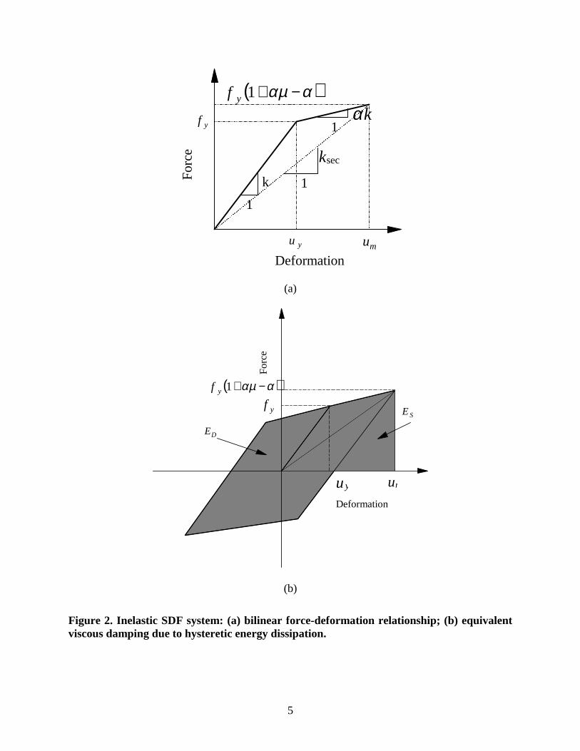
Consider an inelastic SDF system with bilinear force-deformation relationship on initialloading (Fig. 2a). The stiffness of the elastic branch is k and that of the yielding branch is kα .The yield strength and yield displacement are denoted by f y and uy , respectively. If the peak

(maximum absolute) deformation of the inelastic system is um , the ductility factor uu ym=µ .

For the bilinear system of Fig. 2a, the natural vibration period of the equivalent linearsystem with stiffness equal to ksec, the secant stiffness, is

4

α−αµ+µ=

1TT neq

(2)

where Tn is the natural vibration period of the system vibrating within its linearly elastic range( uu y≤ ).

The most common method for defining equivalent viscous damping is to equate theenergy dissipated in a vibration cycle of the inelastic system and of the equivalent linear system.Based on this concept, it can be shown that the equivalent viscous damping ratio is (Chopra,1995: Section 3.9)

E

E

S

Deq π

=ζ4

1 (3)

where the energy dissipated in the inelastic system is given by the area ED enclosed by the

hysteresis loop (Fig. 2b) and 2/2secukE mS = is the strain energy of the system with stiffness ksec

(Fig. 2b). Substituting forED and ES in Eq. (3) leads to

( )( )( )α−αµ+µ

α−−µπ

=ζ1

112eq

(4)

The total viscous damping of the equivalent linear system is

ζ+ζ=ζ eqeqˆ (5)

where ζ is the viscous damping ratio of the bilinear system vibrating within its linearly elasticrange ( uu y≤ ).

For elastoplastic systems, 0=α and Eqs. (2) and (4) reduce to

µ= TT neq µ−µ

π=ζ

12eq

(6)

Equations (2) and (4) are plotted in Fig. 3 where the variation of TT neq and ζeq with µis shown for four values of α . For yielding systems (µ > 1), Teq is longer than Tn and ζeq> 0.

The period of the equivalent linear system increases monotonically with µ for all α . For a fixed

µ , Teq is longest for elastoplastic systems and is shorter for systems with α > 0. For α = 0, ζeq

increases monotonically with µ but not for α > 0. For the latter case, ζeq reaches its maximum

value at a µ value, which depends on α, and then decreases gradually.

5

muyu

yf

Deformation

For

ce1

1

1

kα

ksec

k

( )ααµ −+1f y

(a)

DE

SE

Deformation

For

ce

f y

( )ααµ −+1f y

umuy

(b)

Figure 2. Inelastic SDF system: (a) bilinear force-deformation relationship; (b) equivalentviscous damping due to hysteretic energy dissipation.

6

0 1 2 3 4 5 6 7 8 9 100

0.5

1

1.5

2

2.5

3

3.5

4

µ

Teq

÷ T

n

α = 0

0.050.1

0.2

(a)

0 1 2 3 4 5 6 7 8 9 100

0.1

0.2

0.3

0.4

0.5

0.6

0.7

µ

ζ eq

α = 0

0.05

0.1

0.2

(b)

Figure 3. Variation of period and viscous damping of the equivalent linear system withductility.

7

ATC-40 ANALYSIS PROCEDURES

Contained in the ATC-40 report are approximate analysis procedures to estimate theearthquake-induced deformation of an inelastic system. These procedures are approximate in thesense that they avoid dynamic analysis of the inelastic system. Instead dynamic analyses of asequence of equivalent linear systems with successively updated values of Teq and ζ̂eq

provide a

basis to estimate the deformation of the inelastic system; Teq is determined by Eq. (2) but ζ̂eqby

a modified version of Eq. (5):

ζκ+ζ=ζ eqeqˆ (7)

with ζeq limited to 0.45. Although the basis for selecting this upper limit on damping is not

stated explicitly, ATC-40 states that “The committee who developed these damping coefficientsconcluded that spectra should not be reduced to this extent at higher values and judgmentally …set an absolute limit on … [ ζ+05.0 eq] of about 50 percent.”

0 0.1 0.2 0.3 0.4 0.5 0.60

0.2

0.4

0.6

0.8

1

1.2

ζeq

κ

Type A

Type B

Type C

Figure 4. Variation of damping modification factor with equivalent viscous damping.

The damping modification factor, κ , based primarily on judgment, depends on thehysteretic behavior of the system, characterized by one of three types: Type A denotes hystereticbehavior with stable, reasonably full hysteresis loops, whereas Type C represents severelypinched and/or degraded loops; Type B denotes hysteretic behavior intermediate between TypesA and C. ATC-40 contains equations for κ as a function of ζeq computed by Eq. (3) for the

three types of hysteretic behavior. These equations, plotted in Fig. 4, were designed to ensurethat κ does not exceed an upper limit, a requirement in addition to the limit of 45% on ζeq .

8

ATC-40 states that “… they represent the consensus opinion of the product development team.”Concerned with bilinear systems, this paper will use the κ specified for Type A systems.

ATC-40 specifies three different procedures to estimate the earthquake-induceddeformation demand, all based on the same underlying principles, but differing inimplementation. Procedures A and B are analytical and amenable to computer implementation,whereas procedure C is graphical and most suited for hand analysis. Designed to be the mostdirect application of the methodology, Procedure A is suggested to be the best of the threeprocedures. The capacity diagram is assumed to be bilinear in Procedure B. The description ofProcedures A and B that follows is equivalent to that in the ATC-40 report except that it isspecialized for bilinear systems.

PROCEDURE A

This procedure in the ATC-40 report is described herein as a sequence of steps:

1. Plot the force-deformation diagram and the 5%-damped elastic response (or design) diagram,both in the DA− format to obtain the capacity diagram and 5%-damped elastic demanddiagram, respectively.

2. Estimate the peak deformation demand Di and determine the corresponding pseudo-acceleration Ai from the capacity diagram. Initially, assume %)5,( =ζ= TDD ni , determinedfor period Tn from the elastic demand diagram.

3. Compute ductility uD yi ÷=µ .

4. Compute the equivalent damping ratio ζ̂eq from Eq. (7).

5. Plot the elastic demand diagram for ζ̂eq determined in Step 4 and read-off the displacement

D j where this diagram intersects the capacity diagram.

6. Check for convergence. If ≤÷− DDD jij )( tolerance (=0.05) then the earthquake induced

deformation demand DD j= . Otherwise, set DD ji = (or another estimated value) and repeat

Steps 3-6.

Examples: Specified Ground Motion

This procedure is used to compute the earthquake-induced deformation of the sixexample systems listed in Table 1. Considered are two values of Tn : 0.5s in the acceleration-sensitive spectral region and 1s in the velocity-sensitive region, and three levels of yield strength;ζ=5% for all systems. The excitation chosen is the north-south component of the El Centroground motion; the particular version used is from Chopra (1995). Implementation details arepresented next for selected systems and final results for all systems in Table 2.

The procedure is implemented for System 5 (Table 1).

1. Implementation of Step 1 gives the 5%-damped elastic demand diagram and the capacitydiagram in Fig. 5a.

9

2. Assume cm27.11%)5,0.1( == DDi .

3. 40.4562.227.11 =÷=µ .

4. ( ) 49.040.4140.4637.0 =÷−×=ζeq ; instead use the maximum allowable value 0.45. For

45.0=ζeq and Type A systems (Fig. 4), 77.0=κ and ζκ+ζ=ζ eqeqˆ 45.077.005.0 ×+=

397.0= .

5. The elastic demand diagram for 39.7% damping intersects the capacity diagram atcm725.3=D j (Fig. 5a).

6. DDD jij ÷−× )(100 = ( ) %6.202725.327.11725.3100 −=÷−× > 5% tolerance. Set

cm725.3=Di and repeat Steps 3 to 6.

For the second iteration, cm725.3=Di , 45.1562.2725.3 =÷=µ ,

( ) 198.045.1145.1637.0 =÷−×=ζeq , κ= 0.98, and 243.0ˆ =ζeq. The intersection point

cm654.5=D j and the difference between Di and D j = 34.1% which is greater than the 5%

tolerance. Therefore, additional iterations are required; results of these iterations are summarizedin Table 3. Error becomes less than the 5% tolerance at the end of sixth iteration and theprocedure could have been stopped there. However, the procedure was continued until the errorbecame practically equal to zero. The deformation demand at the end of the iteration process,

cm458.4=D j . Determined by response history analysis (RHA) of the inelastic system,

cm16.10=Dexact and the error = ( ) 16.1016.10458.4100 ÷−× = -56.1%.

Fig. 5b shows the convergence behavior of the ATC-40 Procedure A for System 5.Observe that this iterative procedure converges to a deformation much smaller than the exactvalue. Thus convergence here is deceptive because it can leave the erroneous impression that thecalculated deformation is accurate. In contrast, a rational iterative procedure should lead to theexact result after a sufficient number of iterations.

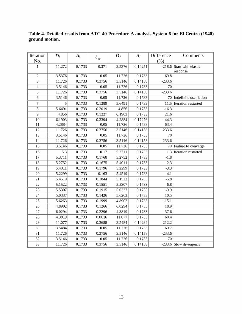
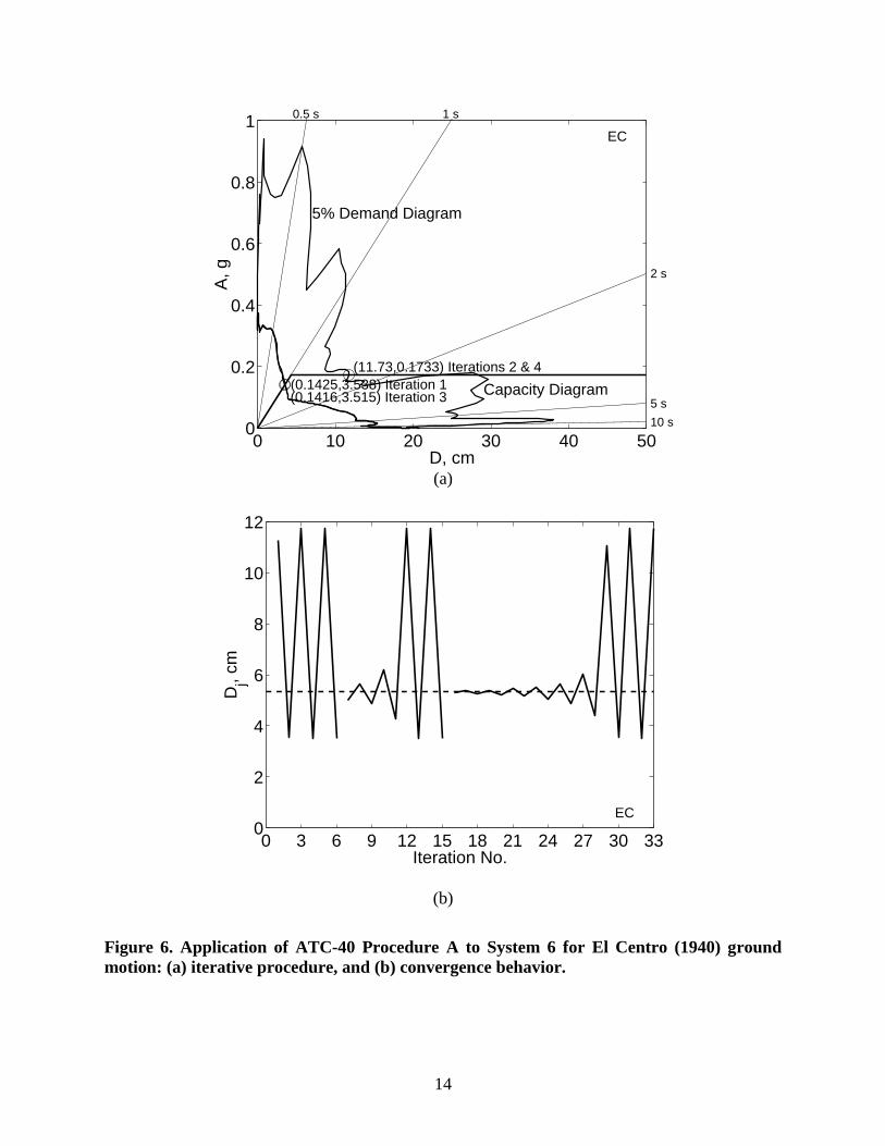
The procedure is next implemented for System 6 (Table 1).

1. Implementation of Step 1 gives the 5%-damped elastic demand diagram and capacitydiagram in Fig. 6a.

2. Assume cm27.11%)5,0.1( == DDi .

3. 62.2302.427.11 =÷=µ .

4. ( ) 39.062.2162.2637.0 =÷−×=ζeq . For 39.0=ζeq and Type A systems (Fig. 4),

82.0=κ and 371.039.082.005.0ˆ =×+=ζκ+ζ=ζ eqeq.

5. The elastic demand diagram for 37.1% damping intersects the capacity diagram atcm538.3=D j (Fig. 6a).


cm538.3=Di and repeat Steps 3 to 6.

10

The results for subsequent iterations, summarized in Table 4, indicate that the procedurefails to converge for this example. In the first iteration, the 37.1%-damped elastic demanddiagram intersects the capacity diagram in its linear-elastic region (Fig. 6a). In subsequentiterations, the intersection point alternates between 11.73 cm and 3.515 cm (Table 4 and Fig. 6b).In order to examine if the procedure would converge with a new starting point, the procedurewas restarted with cm5=Di at iteration number 7. However, the procedure diverges veryquickly as shown by iterations 7 to 15 (Table 4 and Fig. 6b), ending in an alternating pattern.

Table 1. Properties of example systems and their response to El Centro (1940) groundmotion.

System Properties System ResponseSystem Tn

(s)wf y ÷ uy

(cm)µ Dexact

(cm)1 0.1257 0.7801 6 4.6542 0.1783 1.106 4 4.4023

0.5

0.3411 2.117 2 4.2104 0.07141 1.773 6 10.555 0.1032 2.562 4 10.166

1

0.1733 4.302 2 8.533

Table 2. Results from ATC-40 Procedure A analysis of six systems for El Centro (1940)ground motion.

System Converged(?)

Dapprox

(cm)Dexact

(cm)Error(%)

1 Yes 3.534 4.654 -24.12 Yes 3.072 4.402 -30.23 No -- 4.210 --4 Yes 7.912 10.55 -25.05 Yes 4.458 10.16 -56.16 No -- 8.533 --

11

Table 3. Detailed results from ATC-40 Procedure A analysis of System 5 for El Centro(1940) ground motion.

IterationNo.

Di Ai ζ̂ eqD j Aj Difference

(%)

1 11.272 0.1032 0.3965 3.7252 0.1032 -202.62 3.7252 0.1032 0.2432 5.6537 0.1032 34.13 5.6537 0.1032 0.3466 4.0832 0.1032 -38.54 4.0832 0.1032 0.2732 4.7214 0.1032 13.55 4.7214 0.1032 0.3114 4.3523 0.1032 -8.56 4.3523 0.1032 0.2912 4.5002 0.1032 3.37 4.5002 0.1032 0.2999 4.4425 0.1032 -1.38 4.4425 0.1032 0.2966 4.4639 0.1032 0.59 4.4639 0.1032 0.2978 4.4561 0.1032 -0.210 4.4561 0.1032 0.2974 4.4589 0.1032 0.111 4.4589 0.1032 0.2975 4.4579 0.1032 0

12

0 10 20 30 40 500

0.2

0.4

0.6

0.8

1

D, cm

A, g

0.5 s 1 s

2 s

5 s10 s

Capacity Diagram

5% Demand Diagram

(11.27,0.4541)

(11.27,0.1032)

(3.725,0.1032)

39.7% Demand Diagram (1st Iteration)

(4.458,0.1032)

29.7% Demand Diagram (Last Iteration)

EC

(a)

0 2 4 6 8 10 120

2

4

6

8

10

12

Iteration No.

Dj, c

m

Exact

EC

(b)

Figure 5. Application of ATC-40 Procedure A to System 5 for El Centro (1940) groundmotion: (a) iterative procedure, and (b) convergence behavior.

13

Table 4. Detailed results from ATC-40 Procedure A analysis System 6 for El Centro (1940)ground motion.

IterationNo.

Di Ai ζ̂eqD j Aj Difference

(%)Comments

1 11.272 0.1733 0.371 3.5376 0.14251 -218.6 Start with elasticresponse

2 3.5376 0.1733 0.05 11.726 0.1733 69.83 11.726 0.1733 0.3756 3.5146 0.14158 -233.64 3.5146 0.1733 0.05 11.726 0.1733 705 11.726 0.1733 0.3756 3.5146 0.14158 -233.66 3.5146 0.1733 0.05 11.726 0.1733 70 Indefinite oscillation

7 5 0.1733 0.1389 5.6491 0.1733 11.5 Iteration restarted8 5.6491 0.1733 0.2019 4.856 0.1733 -16.39 4.856 0.1733 0.1227 6.1903 0.1733 21.610 6.1903 0.1733 0.2394 4.2884 0.17276 -44.311 4.2884 0.1733 0.05 11.726 0.1733 63.412 11.726 0.1733 0.3756 3.5146 0.14158 -233.613 3.5146 0.1733 0.05 11.726 0.1733 7014 11.726 0.1733 0.3756 3.5146 0.14158 -233.615 3.5146 0.1733 0.05 11.726 0.1733 70 Failure to converge

16 5.3 0.1733 0.17 5.3711 0.1733 1.3 Iteration restarted17 5.3711 0.1733 0.1768 5.2752 0.1733 -1.818 5.2752 0.1733 0.1675 5.4011 0.1733 2.319 5.4011 0.1733 0.1796 5.2299 0.1733 -3.320 5.2299 0.1733 0.163 5.4519 0.1733 4.121 5.4519 0.1733 0.1844 5.1522 0.1733 -5.822 5.1522 0.1733 0.1551 5.5307 0.1733 6.823 5.5307 0.1733 0.1915 5.0337 0.1733 -9.924 5.0337 0.1733 0.1426 5.6263 0.1733 10.525 5.6263 0.1733 0.1999 4.8902 0.1733 -15.126 4.8902 0.1733 0.1266 6.0294 0.1733 18.927 6.0294 0.1733 0.2296 4.3819 0.1733 -37.628 4.3819 0.1733 0.0616 11.077 0.1733 60.429 11.077 0.1733 0.3688 3.5484 0.14294 -212.230 3.5484 0.1733 0.05 11.726 0.1733 69.731 11.726 0.1733 0.3756 3.5146 0.14158 -233.632 3.5146 0.1733 0.05 11.726 0.1733 7033 11.726 0.1733 0.3756 3.5146 0.14158 -233.6 Slow divergence

14

0 10 20 30 40 500

0.2

0.4

0.6

0.8

1

D, cm

A, g

0.5 s 1 s

2 s

5 s

10 s

Capacity Diagram

5% Demand Diagram

(11.73,0.1733) Iterations 2 & 4(0.1425,3.538) Iteration 1(0.1416,3.515) Iteration 3

EC

(a)

0 3 6 9 12 15 18 21 24 27 30 330

2

4

6

8

10

12

Iteration No.

Dj, c

m

EC

(b)

Figure 6. Application of ATC-40 Procedure A to System 6 for El Centro (1940) groundmotion: (a) iterative procedure, and (b) convergence behavior.

15

Examples: Design Spectrum

The ATC-40 Procedure A is next implemented to analyze systems with the excitationspecified by a design spectrum. For illustration we have selected the design spectrum of Fig. 7,which is the median-plus-one-standard-deviation spectrum constructed by the procedures ofNewmark and Hall (1982), as described in Chopra (1995; Section 6.9). The systems analyzedhave the same Tn as those considered previously but their yield strengths for the selected µvalues were determined from the design spectrum (Table 5). Implementation details arepresented next for selected systems and the final results for all systems in Table 6.

0.02 0.05 0.1 0.2 0.5 1 2 5 10 20 500.002

0.005

0.01

0.02

0.05

0.1

0.2

0.5

1

2

5

10

Tn, s

A, g

a

Ta = 1/33 sec

b

Tb = 0.125 sec

c

Tc

d

Td

e

Te = 10 sec

f

Tf = 33 sec

AccelerationSensitive

VelocitySensitive

DisplacementSensitive

Figure 7. Newmark-Hall elastic design spectrum.

The procedure is implemented for System 5 (Table 5).


2. Assume cm64.44%)5,0.1( == DDi .

3. 416.1164.44 =÷=µ .

4. ( ) 48.00.410.4637.0eq =÷−×=ζ ; instead use the maximum allowable value 0.45. For

45.0=ζeq and Type A systems (Fig. 4), 77.0=κ and ζκ+ζ=ζ eqeqˆ 45.077.005.0 ×+=

397.0= .

16

5. The elastic demand diagram for 39.7% damping intersects the capacity diagram atcm18.28Dj = (Fig. 8a).

6. DDD jij ÷−× )(100 = ( ) %4.5818.2864.4418.28100 −=÷−× >5% tolerance. Set =Di 28.18

cm and repeat Steps 3 to 6.

For the second iteration, cm18.28Di = , 52.216.1118.28 =÷=µ ,

( ) 38.052.2152.2637.0eq =÷−×=ζ , κ= 0.84, and 37.0ˆeq

=ζ . The intersection point

cm55.31=D j and the difference between Di and D j = 10.7% which is greater than the 5%

tolerance. Therefore, additional iterations are required; results of these iterations are summarizedin Table 7. The error becomes less than the 5% tolerance at the end of fourth iteration and theprocedure could have been stopped there. However, the procedure was continued till the errorbecame practically equal to zero. The deformation demand at the end of the iteration process is

cm44.30=D j .

Determined directly from the inelastic design spectrum, constructed by the procedures ofNewmark and Hall (1982), as described in Chopra (1995, Section 7.10), the “reference” value ofdeformation is cm64.44=Dspectrum and the discrepancy = ( ) 64.4464.4444.30100 ÷−× = -31.8%.

Fig. 8b shows the convergence behavior of the ATC-40 Procedure A for System 5.Observe that the iterative procedure converges to a deformation value much smaller than the“reference” value.

The procedure is next implemented for System 6 (Table 5).


2. Assume cm64.44%)5,5.0( == DDi .

3. 0.232.2264.44 =÷=µ .

4. ( ) 32.00.210.2637.0eq =÷−×=ζ . For 32.0eq =ζ and Type A systems (Fig. 4), 87.0=κ and

33.032.087.005.0ˆeqeq

=×+=ζκ+ζ=ζ .

5. The elastic demand diagram for 33% damping intersects the capacity diagram atcm56.18Dj = (Fig. 9a).


cm56.18Di = and repeat Steps 3 to 6.

The results for subsequent iterations, summarized in Table 8, indicate that the procedurefails to converge for this example. In the first iteration, the 33%-damped elastic demand diagramintersects the capacity diagram in its linear-elastic region (Fig. 9a). In subsequent iterations, theintersection point alternates between 13.72 cm and 89.28 cm (Table 8 and Fig. 9b). In order toexamine if the procedure would converge with a new starting point, the procedure was restartedwith cm28Di = at iteration number 6. However, the procedure diverges very quickly as shownby iterations 6 to 11 (Table 8 and Fig. 9b), ending in an alternating pattern.

17

Table 5. Properties of example systems and their deformations from inelastic designspectrum.

System Properties System ResponseSystem Tn

(s)wf y ÷ uy

(cm)µ Dspectrum

(cm)1 0.5995 3.7202 6 22.322 0.8992 5.5803 4 22.323

0.5

1.5624 9.6962 2 19.394 0.2997 7.4403 6 44.645 0.4496 11.160 4 44.646

1

0.8992 22.321 2 44.64

Table 6. Results from ATC-40 Procedure A analysis of six systems for design spectrum.

System Converged(?)

Dapprox

(cm)Dspectrum

(cm)Discrepancy

(%)1 No -- 22.32 --2 No -- 22.32 --3 No -- 19.39 --4 No -- 44.64 --5 Yes 30.44 44.64 -31.86 Yes 42.28 44.64 -5.3

Table 7. Detailed results ATC-40 Procedure A analysis of System 5 for design spectrum.

IterationNo.

Di Ai ζ̂ eqD j Aj Difference

(%)

1 44.64 0.4496 0.3965 28.18 0.4496 -58.42 28.18 0.4496 0.3664 31.55 0.4496 10.73 31.54 0.4496 0.3796 30.01 0.4496 -5.14 30.01 0.4496 0.3741 30.64 0.4496 25 30.64 0.4496 0.3764 30.37 0.4496 -0.96 30.36 0.4496 0.3754 30.48 0.4496 0.47 30.48 0.4496 0.3759 30.43 0.4496 -0.28 30.43 0.4496 0.3757 30.45 0.4496 0.19 30.45 0.4496 0.3757 30.44 0.4496 0

18

0 50 100 150 2000

1

2

3

D, cm

A, g

5% Demand Diagram

0.5 s 1 s

2 s

5 s

10 s

(44.64,1.798)

Capacity Diagram(44.64,0.4492)

(28.18,0.4492)(30.44,0.4492)

39.7% Demand Diagram (1st Iteration)37.6% Demand Diagram (Last Iteration)

NH

(a)

0 2 4 6 8 100

10

20

30

40

50

Iteration No.

Dj, c

m

Inelastic Design Spectrum

NH

(b)

Figure 8. Application of ATC-40 Procedure A to Example 5 for elastic design spectrum: (a)iterative procedure, and (b) convergence behavior.

19

Table 8. Detailed results ATC-40 Procedure A analysis of System 6 for design spectrum.

IterationNo.

Di Ai ζ̂eqD j Aj Difference

(%)Comments

1 44.64 0.8992 0.3288 18.56 0.7475 -140.6 Start with elastic response2 18.56 0.8992 0.0500 89.28 0.8992 79.23 89.28 0.8992 0.3965 13.72 0.5527 -550.74 13.72 0.8992 0.0500 89.28 0.8992 84.65 89.28 0.8992 0.3965 13.72 0.5527 -550.7 Indefinite oscillation

6 28.00 0.8992 0.1792 35.27 0.8992 20.6 Iteration restarted7 35.27 0.8992 0.2705 23.10 0.8992 -52.78 23.10 0.8992 0.0715 71.67 0.8992 67.89 71.67 0.8992 0.3917 14.03 0.5653 -410.710 14.03 0.8992 0.0500 89.28 0.8992 84.311 89.28 0.8992 0.3965 13.72 0.5527 -550.7 Indefinite oscillation

12 29.00 0.8992 0.1967 32.29 0.8992 10.2 Iteration restarted13 32.29 0.8992 0.2413 26.23 0.8992 -23.114 26.23 0.8992 0.1449 42.56 0.8992 38.415 42.56 0.8992 0.3189 19.34 0.7791 -120.116 19.34 0.8992 0.0500 89.28 0.8992 78.317 89.28 0.8992 0.3965 13.72 0.5527 -550.718 13.72 0.8992 0.0500 89.28 0.8992 84.619 89.28 0.8992 0.3965 13.72 0.5527 -550.7 Slow divergence

20

0 50 100 150 2000

1

2

3

D, cm

A, g

5% Demand Diagram

0.5 s 1 s

2 s

5 s

10 s

Capacity Diagram(18.56,0.7475) Iteration 1

(89.28,0.8992) Iterations 2 & 4

(13.72,0.5527) Iterations 3 & 5

NH

(a)

0 2 4 6 8 10 12 14 16 18 200

20

40

60

80

100

Iteration No.

Dj, c

m

NH

(b)

Figure 9. Application of ATC-40 Procedure A to System 6 for elastic design spectrum: (a)iterative procedure, and (b) convergence behavior.

21

PROCEDURE B

This procedure in the ATC-40 report is described herein as a sequence of steps:

1. Plot the capacity diagram.

2. Estimate the peak deformation demand Di . Initially assume %)5,( =ζ= TDD ni .

3. Compute ductility uD yi ÷=µ .

4. Compute equivalent period Teq and damping ratio ζ̂eq from Eqs. (2) and (7), respectively.

5. Compute the peak deformation )ˆ,( ζeqeqTD and peak pseudo-acceleration )ˆ,( ζeqeqTA of an

elastic SDF system with vibration properties Teq and ζ̂eq.

6. Plot the point with coordinates )ˆ,( ζeqeqTD and )ˆ,( ζeqeqTA .

7. Check if the curve generated by connecting the point plotted in Step 6 to previouslydetermined, similar points intersects the capacity diagram. If not, repeat Steps 3-7 with a newvalue of Di ; otherwise go to Step 8.

8. The earthquake-induced deformation demand is given by the D -value at the intersectionpoint.

Examples: Specified Ground Motion

Procedure B is implemented for the Systems 1 to 6 (Table 1). The final results aresummarized in Table 9; details are presented next. For a number of assumed values of µ (or D),pairs of values )ˆ,( ζeqeqTD and )ˆ,( ζeqeqTA are generated (Tables 10 and 11). These pairs are

plotted to obtain the curve A-B in Fig. 10, wherein capacity diagrams for three systems areshown together with the 5%-damped linear elastic demand diagram; the latter need not beplotted. The intersection point between the curve A-B and the capacity diagram of a system givesits deformation demand: cm536.3=D , cm075.3=D , and cm284.3=D for Systems 1 to 3,respectively (Fig. 10a); and cm922.7D = , cm454.4=D , and cm318.5=D for Systems 4 to6, respectively (Fig. 10b). In contrast, the exact deformations computed by RHA of the inelasticsystems are 4.654 cm, 4.402 cm, and 4.210 cm for Systems 1 to 3; and 10.55 cm, 10.16 cm, and8.533 cm for Systems 4 to 6, indicating that the error in the approximate procedure ranges from –22% to –56.2%. Observe that the curve A-B provides the information to determine thedeformation demand in several systems with the same Tn values but different yield strengths.

Procedure B always gives a unique estimate of the deformation, whereas, as noted earlier,the iterative Procedure A may not always converge. If it does converge, the two procedures givethe same value of deformation (within round-off and interpolation errors) in the examples solved.

22

Table 9. Results from ATC-40 Procedure B analysis of six systems for El Centro groundmotion.

System Dapprox

(cm)Dexact

(cm)Discrepancy

(%)1 3.536 4.654 -24.02 3.075 4.402 -30.13 3.284 4.210 -22.04 7.922 10.55 -24.95 4.453 10.16 -56.26 5.318 8.533 -37.7

23

Table 10. Detailed results from ATC-40 Procedure B analysis of Systems 1 to 3 for ElCentro (1940) ground motion.

µ Teq ζ̂ eqD A

1 0.5 0.05 5.6846 0.915991.1 0.5244 0.1079 4.411 0.646161.2 0.5477 0.1562 4.0093 0.538371.3 0.5701 0.197 3.7297 0.462291.4 0.5916 0.2292 3.5032 0.403211.5 0.6124 0.2539 3.3449 0.35933

1.55 0.6225 0.2646 3.2859 0.34161.5515 0.6228 0.2649 3.2842 0.34111.5531 0.6228 0.2649 3.2854 0.34085

1.6 0.6325 0.2743 3.228 0.32511.7 0.6519 0.2914 3.1162 0.295371.8 0.6708 0.3058 3.0093 0.269391.9 0.6892 0.3182 2.9207 0.2477

2 0.7071 0.3288 2.8739 0.231552.1 0.7246 0.338 2.898 0.222372.2 0.7416 0.3461 2.9204 0.21392.3 0.7583 0.3532 2.9412 0.206062.4 0.7746 0.3595 2.9605 0.198772.5 0.7906 0.365 2.9929 0.192912.6 0.8062 0.37 3.024 0.187422.7 0.8216 0.3745 3.0531 0.18221

2.7787 0.8335 0.3778 3.0747 0.17832.8 0.8367 0.3786 3.0804 0.177272.9 0.8515 0.3823 3.1058 0.17257

3 0.866 0.3856 3.1295 0.168093.1 0.8803 0.3887 3.1517 0.163823.2 0.8944 0.3914 3.1723 0.159743.3 0.9083 0.394 3.1992 0.156213.4 0.922 0.3964 3.2273 0.152953.5 0.9354 0.3965 3.2632 0.150233.6 0.9487 0.3965 3.2973 0.147593.7 0.9618 0.3965 3.3293 0.144993.8 0.9747 0.3965 3.359 0.142443.9 0.9874 0.3965 3.3868 0.13993

4 1 0.3965 3.4126 0.137474.1 1.0124 0.3965 3.4366 0.135064.2 1.0247 0.3965 3.4588 0.13274.3 1.0368 0.3965 3.4792 0.130384.4 1.0488 0.3965 3.5023 0.128264.5 1.0607 0.3965 3.528 0.12633

4.525 1.0636 0.3965 3.5342 0.125854.533 1.0645 0.3965 3.5362 0.1257

24

Table 11. Detailed results from ATC-40 Procedure B analysis of Systems 4 to 6 for ElCentro (1940) ground motion.

µ Teq ζ̂ eqD A

1 1 0.05 11.272 0.454071.1 1.0488 0.1079 7.4536 0.272971.2 1.0954 0.1562 5.7066 0.19157

1.225 1.1068 0.167 5.4288 0.17852

1.2362 1.1119 0.1717 5.3182 0.173301.2375 1.1119 0.1717 5.3157 0.17304

1.3 1.1402 0.197 5.0373 0.156091.4 1.1832 0.2292 4.8741 0.140251.5 1.2247 0.2539 4.7401 0.127301.6 1.2649 0.2743 4.6154 0.116201.7 1.3038 0.2914 4.4969 0.10656

1.7384 1.3185 0.2972 4.4535 0.10321.8 1.3416 0.3058 4.3893 0.098231.9 1.3784 0.3182 4.5607 0.09670

2 1.4142 0.3288 4.7224 0.095122.1 1.4491 0.338 4.8831 0.093672.2 1.4832 0.3461 5.0397 0.092282.3 1.5166 0.3532 5.1901 0.090902.4 1.5492 0.3595 5.335 0.089552.5 1.5811 0.365 5.4748 0.088222.6 1.6125 0.37 5.6097 0.086922.7 1.6432 0.3745 5.7401 0.085642.8 1.6733 0.3786 5.8749 0.084522.9 1.7029 0.3823 6.0057 0.08343

3 1.7321 0.3856 6.1323 0.082343.1 1.7607 0.3887 6.2546 0.081283.2 1.7889 0.3914 6.3727 0.080233.3 1.8166 0.394 6.491 0.079243.4 1.8439 0.3964 6.6094 0.078313.5 1.8708 0.3965 6.742 0.077603.6 1.8974 0.3965 6.8714 0.076893.7 1.9235 0.3965 7.0005 0.076223.8 1.9494 0.3965 7.1297 0.075583.9 1.9748 0.3965 7.2543 0.07493

4 2 0.3965 7.3773 0.074304.1 2.0248 0.3965 7.501 0.073704.2 2.0494 0.3965 7.6197 0.073084.3 2.0736 0.3965 7.7332 0.072454.4 2.0976 0.3965 7.8442 0.07182

4.45 2.1095 0.3965 7.9008 0.07152

4.4688 2.114 0.3965 7.9217 0.07141

25

0 10 20 30 40 500

0.2

0.4

0.6

0.8

1

D, cm

A, g

0.5 s 1 s

2 s

5 s

10 s

5% Demand Diagram

A

B(3.536,0.1257)

(3.284,0.3411)

(3.075,0.1783)

EC

(a)

0 10 20 30 40 500

0.2

0.4

0.6

0.8

1

D, cm

A, g

0.5 s 1 s

2 s

5 s

10 s

5% Demand Diagram

A

B

(5.318,0.1733)

(7.922,0.07141)

(4.454,0.1032)

EC

(b)

Figure 10. Application of ATC-40 Procedure B for El Centro (1940) ground motion: (a)Systems 1 to 3, and (b) Systems 4 to 6.

26

Examples: Design Spectrum

Procedure B is implemented for the Systems 1 to 6 (Table 5). The results from thisprocedure are summarized in Table 12 and illustrated in Fig. 11 where the estimateddeformations are noted; intermediate results are available in Tables 13 and 14. Theseapproximate values are compared in Table 12 against the values determined directly from theinelastic design spectrum constructed by the procedure of Newmark and Hall (1982), asdescribed in Chopra (1995, Section 7.10); see Appendix B for details. Relative to these referencevalues, the discrepancy ranges from –5.2% to –58.6% for the systems considered.

Table 12. Results from ATC-40 Procedure B analysis of six systems for design spectrum.

System Dapprox

(cm)Dspectrum

(cm)Discrepancy

(%)1 10.46 22.32 -53.12 9.245 22.32 -58.63 11.51 19.39 -40.64 42.27 44.64 -5.25 30.45 44.64 -31.76 29.84 44.64 -33.1

Table 13. Detailed results from ATC-40 Procedure B analysis of Systems 1 to 3 for designspectrum.

µ Teq ζ̂ eqD A

1 0.5 0.05 16.794 2.70621.1 0.5244 0.1079 13.012 1.90611.2 0.5477 0.1562 11.332 1.5217

1.1871 0.5448 0.1504 11.51 1.56241.3 0.5701 0.197 10.328 1.28021.4 0.5916 0.2292 9.7547 1.12271.5 0.6124 0.2539 9.4602 1.01631.6 0.6325 0.2743 9.2924 0.9358

1.6567 0.6436 0.2843 9.2447 0.89921.7 0.6519 0.2914 9.2107 0.87301.8 0.6708 0.3058 9.1906 0.82271.9 0.6892 0.3182 9.2164 0.7816

2 0.7071 0.3288 9.2776 0.74752.1 0.7246 0.338 9.3664 0.71872.2 0.7416 0.3461 9.4776 0.69422.3 0.7583 0.3532 9.607 0.67312.4 0.7746 0.3595 9.7515 0.65472.5 0.7906 0.365 9.9087 0.63872.6 0.8062 0.37 10.077 0.62452.7 0.8216 0.3745 10.254 0.61202.8 0.8367 0.3786 10.439 0.6008

2.8123 0.8385 0.3791 10.463 0.5995

27

Table 14. Detailed results from ATC-40 Procedure B analysis of Systems 4 to 6 for designspectrum.

µ Teq ζ̂ eqD A

1 1 0.05 44.642 1.79841.2 1.0954 0.1562 32.69 1.0974

1.3519 1.1627 0.2154 29.84 0.88921.4 1.1832 0.2292 29.411 0.84631.6 1.2649 0.2743 28.488 0.71731.8 1.3416 0.3058 28.32 0.6338

2 1.4142 0.3288 28.521 0.57452.2 1.4832 0.3461 28.926 0.52972.4 1.5492 0.3595 29.448 0.49432.6 1.6125 0.37 30.042 0.4655

2.7283 1.6517 0.3757 30.449 0.44962.8 1.6733 0.3786 30.679 0.4414

3 1.7321 0.3856 31.343 0.42093.2 1.7889 0.3914 32.022 0.40313.4 1.8439 0.3964 32.708 0.38753.6 1.8974 0.3965 33.648 0.37653.8 1.9494 0.3965 34.57 0.3665

4 2 0.3965 35.468 0.35724.2 2.0494 0.3965 36.344 0.34864.4 2.0976 0.3965 37.199 0.34064.6 2.1448 0.3965 38.035 0.33314.8 2.1909 0.3965 38.853 0.3261

5 2.2361 0.3965 39.654 0.31955.2 2.2804 0.3965 40.44 0.31335.4 2.3238 0.3965 41.21 0.30745.6 2.3664 0.3965 41.966 0.3019

5.6822 2.3837 0.3965 42.273 0.2997

28

0 50 100 150 2000

1

2

3

D, cm

A, g

5% Elastic Demand Diagram

0.5 s 1 s

2 s

5 s

10 s

A

B

(11.51,1.56)

(9.245,0.8992)

(10.46,0.5995)

NH

(a)

0 50 100 150 2000

1

2

3

D, cm

A, g


0.5 s 1 s

2 s

5 s

10 s

A

B

(29.84,0.8992)

(30.45,0.4496)

(42.27,0.2997)

NH

(b)

Figure 11. Application of ATC-40 Procedure B for elastic design spectrum: (a) Systems 1 to3, and (b) Systems 4 to 6.

29

EVALUATION OF ATC-40 PROCEDURES

SPECIFIED GROUND MOTION

The ATC-40 Procedure B is implemented for a wide range of system parameters andexcitations in two versions: (1) =κ 1, i.e., the equivalent viscous damping is given by Eqs. (4)and (5) based on well-established principles; and (2) κ is given by Fig. 4, a definition basedprimarily on judgment to account for different types of hysteretic behavior.

The yield strength of each elastoplastic system analyzed was chosen corresponding to anallowable ductility µ :

wgAf yy )(= (8)

where w is the weight of the system and Ay is the pseudo-acceleration corresponding to the

allowable ductility and the vibration properties — natural period Tn and damping ratio ζ — ofthe system in its linear range of vibration. Recall that the ductility demand (computed bynonlinear response history analysis) imposed by the selected ground motion on systems definedin this manner will exactly equal the allowable ductility (Chopra, 1995; Section 19.1.1).

The peak deformation due to a selected ground motion, determined by the ATC-40method, Dapprox , is compared in Fig. 12 against the “exact” value, Dexact , determined by

nonlinear RHA, and the percentage error in the approximate result is plotted in Fig. 13. Thesefigures permit several observations. The approximate procedure is not especially accurate. Itunderestimates significantly the deformation for wide ranges of Tn values with errorsapproaching 50%, implying that the estimated deformation is only about half of the valuedetermined by nonlinear RHA. The approximate method gives larger deformation for shortperiod systems (Tn < 0.1 sec for µ = 2 and Tn < 0.4 sec for µ = 6) and the deformation does notapproach zero as Tn goes to zero. This unreasonable discrepancy occurs because, for very short-period systems with small yield strength, the Teq has to shift to the constant-V region of the

spectrum before the capacity and demand diagrams can intersect (Appendix A). While inclusionof the damping modification factor κ increases the estimated displacement, the accuracy of theapproximate results improves only marginally for the smaller values of µ. Therefore the κ factoris not attractive, especially because it is based primarily on judgement.

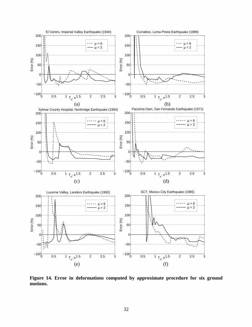
Shown in Fig. 14 are the errors in the ATC-40 method, with the κ factor included, for sixdifferent ground motions: (1) El Centro, S00E, 1940 Imperial Valley; (2) Corralitos, Chan-1, 90deg, 1989 Loma Prieta; (3) Sylmar County Hospital Parking Lot, Chan-3, 360 deg, 1994Northridge; (4) Pacoima Dam, N76W, 1971 San Fernando; (5) Lucerne Valley, S80W, 1992Landers; and (6) SCT, S00E, 1985 Mexico City. Observe that, contrary to intuition, the errordoes not decrease consistently for smaller ductility. While the magnitude of the error and itsvariation with Tn depend on the excitation, the earlier observation that the error in theapproximate method is significant is supported by results for several ground motions.

30

0 0.5 1 1.5 2 2.5 30

5

10

15

20

25

30

Tn, s

D, c

m

ExactATC−40, κ=1ATC−40

µ = 2

EC

(a)

0 0.5 1 1.5 2 2.5 30

5

10

15

20

25

30

Tn, s

D, c

m

ExactATC−40, κ=1ATC−40

µ = 6

EC

(b)

Figure 12. Comparison of deformations due to El Centro (1940) ground motion fromapproximate procedure and nonlinear response history analysis: (a) µ = 2, and (b) µ = 6.

31

0 0.5 1 1.5 2 2.5 3−100

−50

0

50

100

Tn, s

Err

or (

%)

ATC−40, κ=1ATC−40

µ = 2

EC

(a)

0 0.5 1 1.5 2 2.5 3−100

−50

0

50

100

Tn, s

Err

or (

%)

ATC−40, κ=1ATC−40

µ = 6

EC

(b)

Figure 13. Error in deformations due to El Centro (1940) ground motion computed byapproximate procedure: (a) µ = 2, and (b) µ = 6.

32

0 0.5 1 1.5 2 2.5 3−100

−50

0

50

100

150

200

Tn, s

Err

or (

%)

El Centro, Imperial Valley Earthquake (1940)

µ = 2µ = 6

0 0.5 1 1.5 2 2.5 3−100

−50

0

50

100

150

200

Tn, s

Err

or (

%)

Corralitos, Loma Prieta Earthquake (1989)

µ = 2µ = 6

(a) (b)

0 0.5 1 1.5 2 2.5 3−100

−50

0

50

100

150

200

Tn, s

Err

or (

%)

Sylmar County Hospital, Northridge Earthquake (1994)

µ = 2µ = 6

0 0.5 1 1.5 2 2.5 3−100

−50

0

50

100

150

200

Tn, s

Err

or (

%)

Pacoima Dam, San Fernando Earthquake (1971)

µ = 2µ = 6

(c) (d)

0 0.5 1 1.5 2 2.5 3−100

−50

0

50

100

150

200

Tn, s

Err

or (

%)

Lucerne Valley, Landers Earthquake (1992)

µ = 2µ = 6

0 0.5 1 1.5 2 2.5 3−100

−50

0

50

100

150

200

Tn, s

Err

or (

%)

SCT, Mexico City Earthquake (1985)

µ = 2µ = 6

(e) (f)

Figure 14. Error in deformations computed by approximate procedure for six groundmotions.

33

DESIGN SPECTRUM

The ATC-40 Procedure B is implemented for a wide range of Tn and µ values with theexcitation characterized by the elastic design spectrum of Fig. 7. The yield strength was definedby Eq. (8) with Ay determined from the inelastic design spectrum corresponding to the selected

ductility factor. The resulting approximate values of deformations will be compared in thissection with those determined directly from the design spectrum, as described next.

Given the properties Tn , ζ, f y and α of the bilinear hysteretic system and the elastic

design spectrum, the earthquake-induced deformation of the system can be determined directlyfrom the design spectrum. The peak deformation D of this system is given by

DD yµ= (9)

with the yield deformation defined by

AT

D yn

y

π=

2

2 (10)

where Ay is the pseudo-acceleration related to the yield strength, f y , by Eq. (8). Putting Eqs.

(9) and (10) together gives

ATD y

n

πµ=

2

2 (11)

The yield strength reduction factor is given by

A

A

f

fR

yy

oy ==

(12)

where

wg

Af o

=(13)

is the minimum yield strength required for the structure to remain elastic; A is the pseudo-acceleration ordinate of the elastic design spectrum at ),( ζTn . Substituting Eq. (12) in Eq. (11)gives

AT

RD n

y

πµ=

2

12 (14)

Equation (14) provides a convenient way to determine the deformation of the inelastic systemfrom the design spectrum. All that remains to be done is to determine µ for a given Ry ; the latter

is known from Eq. (12) for a structure with known f y .

34

Presented in Fig. 15 are the deformations determined by Eq. 14 using three differentTR ny −µ− equations: Newmark and Hall (1982); Krawinkler and Nassar (1992) for

elastoplastic systems; and Vidic, Fajfar and Fischinger (1994) for bilinear systems. Theequations describing these relationships are presented later in this report. Observe that the threerecommendations lead to similar results except for sec3.0<Tn , indicating that the inelasticdesign spectrum is a reliable approach to estimate the earthquake-induced deformation ofyielding systems.

0.05 0.1 0.2 0.5 1 2 5 10 20 500.10.2

0.512

51020

50100200

500

Tn, s

D, c

m NH

KN

VFF


VelocitySensitive


µ = 4

Figure 15. Deformation of inelastic systems (µ= 4) determined from inelastic design spectrausing three TR ny −µ− equations: Newmark-Hall (NH), Krawinkler-Nassar (KN), andVidic-Fajfar-Fischinger (VFF).

The deformation estimates by the ATC-40 method are compared in Fig. 16 with thosefrom inelastic design spectra presented in Fig. 15. Relative to these “reference” values, thepercentage discrepancy in the approximate result is plotted in Fig. 17. The results of Figs. 16 and17 permit the following observations. The approximate procedure leads to significantdiscrepancy, except for very long periods ( TT fn > in Fig. 7). The magnitude of this discrepancy

depends on the design ductility and the period region. In the acceleration-sensitive )( TT cn < and

displacement-sensitive )( TTT fd n << regions (Fig. 7), the approximate procedure significantly

underestimates the deformation; the discrepancy increases with increasing µ. In the velocity-sensitive )( TTT dc n << region, the ATC-40 procedure significantly underestimates the

deformation for µ = 2 and 4, but overestimates it for µ = 8 and is coincidentally accurate forµ = 6.

35

In passing, note that the ATC-40 procedure is deficient relative to even the elastic designspectrum in the velocity-sensitive and displacement-sensitive regions )( TT cn > . For Tn in these

regions, the peak deformation of an inelastic system can be estimated from the elastic designspectrum, using the well-known equal-displacement rule (Veletsos and Newmark, 1960).However, the ATC-40 procedure requires analyses of several equivalent linear systems and stillproduces worse results.

36

0.05 0.1 0.2 0.5 1 2 5 10 20 500.10.2

0.512

51020

50100200

500

Tn, s

D, c

m

Design Spectrum (NH)

ATC−40


VelocitySensitive


µ = 4

(a)

0.05 0.1 0.2 0.5 1 2 5 10 20 500.10.2

0.512

51020

50100200

500

Tn, s

D, c

m

Design Spectrum (KN)

ATC−40


VelocitySensitive


µ = 4

(b)

0.05 0.1 0.2 0.5 1 2 5 10 20 500.10.2

0.512

51020

50100200

500

Tn, s

D, c

m

Design Spectrum (VFF)

ATC−40


VelocitySensitive


µ = 4

(c)

Figure 16. Comparison of deformations computed by ATC-40 procedure with those fromthree different inelastic design spectra (µ = 4): (a) Newmark and Hall (1982), (b)Krawinkler and Nassar (1992), and (c) Vidic, Fajfar and Fischinger (1994).

37

0.05 0.1 0.2 0.5 1 2 5 10 20 50−100

−50

0

50

100

Tn, s

Dis

crep

ancy

(%

) µ = 2µ = 4µ = 6µ = 8


VelocitySensitive


NH

(a)

0.05 0.1 0.2 0.5 1 2 5 10 20 50−100

−50

0

50

100

Tn, s

Dis

crep

ancy

(%

) µ = 2µ = 4µ = 6µ = 8


VelocitySensitive


KN

(b)

0.05 0.1 0.2 0.5 1 2 5 10 20 50−100

−50

0

50

100

Tn, s

Dis

crep

ancy

(%

) µ = 2µ = 4µ = 6µ = 8


VelocitySensitive


VFF

(c)

Figure 17. Discrepancy in deformations computed by ATC-40 procedure relative to threedifferent inelastic design spectra: (a) Newmark and Hall (1982), (b) Krawinkler and Nassar(1992), and (c) Vidic, Fajfar and Fischinger (1994).

38

IMPROVED PROCEDURES

Presented next are two improved procedures that eliminate the errors (or discrepancies) inthe ATC-40 procedures, but retain their graphical appeal. Procedures A and B that are presentedare akin to ATC-40 Procedures A and B, respectively. The improved procedures use the well-known constant-ductility design spectrum for the demand diagram, instead of the elastic designspectrum for equivalent linear systems in ATC-40 procedures.

INELASTIC DESIGN SPECTRUM

A constant-ductility design spectrum is established by reducing the elastic designspectrum by appropriate ductility-dependent factors that depend on Tn . The earliestrecommendation for the reduction factor, Ry (Eq. 12), goes back to the work of Veletsos andNewmark (1960), which is the basis for the inelastic design spectra developed by Newmark andHall (1982). Starting with the elastic design spectrum of Fig. 7 and these µ−Ry relations foracceleration-, velocity-, and displacement-sensitive spectral regions, the inelastic designspectrum constructed by the procedure described in Chopra (1995, Section 7.10) is shown in Fig.18a.

In recent years, several recommendations for the reduction factor have been developed(Krawinkler and Nassar, 1992; Vidic, Fajfar, and Fischinger, 1994; Riddell, Hidalgo, and Cruz,1989; Tso and Naumoski, 1991; Miranda and Bertero, 1994). Based on two of theserecommendations, the inelastic design spectrum is shown in Figs. 18b and 18c. For a fixed µ = 2,the inelastic spectra from Fig. 18 are compared in Fig. 19. The three spectra are very similar inthe velocity-sensitive region of the spectrum, but differ in the acceleration-sensitive region. Animproved procedure based on such inelastic design spectra is presented in two versions thatfollow.

INELASTIC DEMAND DIAGRAM

The inelastic design spectra of Fig. 18 will be plotted in the A-D format to obtain thecorresponding demand diagrams. The peak deformation D of the inelastic system is given by Eq.(11) where Ay is known from Fig. 18 for a given Tn and µ. Determined corresponding to the

three inelastic design spectra in Fig. 18, such data pairs (Ay ,D) are plotted to obtain the demand

diagram for inelastic systems (Fig. 20).

39

0 1 2 3 4 50

0.5

1

1.5

2

2.5

3

Tn, s

Ay, (

g)

µ = 1

2

46

8

1.5

NH

(a)

0 1 2 3 4 50

0.5

1

1.5

2

2.5

3

Tn, s

Ay, (

g)

µ = 1

2

468

1.5

KN

(b)

0 1 2 3 4 50

0.5

1

1.5

2

2.5

3

Tn, s

Ay, (

g)

µ = 1

2

468

1.5

VFF

(c)

Figure 18. Inelastic design spectra: (a) Newmark and Hall (1982), (b) Krawinkler andNassar (1992), and (c) Vidic, Fajfar and Fischinger (1994).

40

0 1 2 3 4 50

0.5

1

1.5

2

2.5

Tn, s

Ay, g

NHKNVFF

µ = 2

Figure 19. Pseudo-acceleration design spectrum for inelastic systems (µ= 2) using threeTR ny −µ− equations: Newmark-Hall (NH), Krawinkler-Nassar (KN), and Vidic-Fajfar-

Fischinger (VFF).

PROCEDURE A

This procedure, which uses the demand diagram for inelastic systems (Fig. 20), will beillustrated with reference to six elastoplastic systems defined by two values of Tn = 0.5 and 1.0sec and three different yield strengths, given by Eq. (8) corresponding to µ = 2, 4, and 6,respectively. Superimposed on the demand diagrams are the capacity diagrams for three inelasticsystems with Tn = 0.5 sec (Figs. 21a, 22a, and 23a) and Tn = 1.0 sec (Figs. 21b, 22b, and 23b).

The yielding branch of the capacity diagram intersects the demand diagram for several µ values.One of these intersection points, which remains to be determined, will provide the deformationdemand. At the one relevant intersection point, the ductility factor calculated from the capacitydiagram should match the ductility value associated with the intersecting demand curve.Determined according to this criterion, the deformation for each system is noted in Figs. 21 to23. Implementation of this procedure is illustrated for two systems.

Examples

The yield deformation of System 1 is uy = cm724.3 . The yielding branch of the capacity

diagram intersects the demand curves for µ = 1, 2, 4, 6, and 8 at 133.93 cm, 66.96 cm, 33.48 cm,22.3 cm, and 16.5 cm, respectively (Fig. 21a). Dividing by uy , the corresponding ductility

factors are 133.93÷3.724=35.96 (which exceeds µ = 1 for this demand curve),66.96÷3.724=17.98 (which exceeds µ = 2 for this demand curve), 33.48÷3.724=8.99 (whichexceeds µ = 4 for this demand curve), 22.3÷3.724=6 (which matches µ = 6 for this demand

41

curve), and 16.5÷3.724=4.43 (which is smaller than µ = 8 for this demand curve). Thus, theductility demand is 6 and the deformation of System 1 is D = 22.3 cm.

For System 3, uy = cm681.9 . The yielding branch of the capacity diagram intersects the

demand curve for µ = 1 at 51.34 cm (Fig. 21a). The corresponding ductility factor is51.34÷9.681=5.3, which is larger than the µ = 1 for this demand curve. The yielding branch ofthe capacity diagram also intersects the demand curve for µ = 2 continuously from 9.681 cm to25.2 cm, which correspond to ductility factors of 1 to 2.6. The intersection point at 19.29 cmcorresponds to ductility factor = 19.39÷9.681=2 which matches µ = 2 for this demand curve.Thus, the ductility demand is 2 and the deformation of System 3 is D = 19.39 cm.

42

0 50 100 150 2000

1

2

3

D, cm

Ay, g

µ = 1

1.5

2

46

8

0.5 s 1 s

2 s

5 s

10 s

NH

(a)

0 50 100 150 2000

1

2

3

D, cm

Ay, g

µ = 1

1.52.0

4.0

6.0

8.0

0.5 s 1 s

2 s

5 s

10 s

KN

(b)

0 50 100 150 2000

1

2

3

D, cm

Ay, g

µ = 1

1.5

2

468

0.5 s 1 s

2 s

5 s

10 s

VFF

(c)

Figure 20. Inelastic demand diagrams: (a) Newmark and Hall (1982), (b) Krawinkler andNassar (1992), and (c) Vidic, Fajfar and Fischinger (1994).

43

0 50 100 150 2000

1

2

3

D, cm

Ay, g

µ = 1

2

46

8

0.5 s 1 s

2 s

5 s

10 s

(19.39,1.562)

(22.32,0.8992)

(22.32,0.5995)

NH

(a)

0 50 100 150 2000

1

2

3

D, cm

Ay, g

µ = 1

2

46

8

0.5 s 1 s

2 s

5 s

10 s

(44.64,0.8992)

(44.64,0.4496)

(44.64,0.2997)

NH

(b)

Figure 21. Application of improved Procedure A using Newmark-Hall (1982) inelasticdesign spectrum: (a) Systems 1 to 3, and (b) Systems 4 to 6.

44

0 50 100 150 2000

1

2

3

D, cm

Ay, g

µ = 1

1.77

3.25

5.14

0.5 s 1 s

2 s

5 s

10 s

(17.2,1.562)

(18.15,0.8992)

(19.11,0.5995)

KN

(a)

0 50 100 150 2000

1

2

3

D, cm

Ay, g

µ = 1

1.97

3.80

5.56

0.5 s 1 s

2 s

5 s

10 s

(43.97,0.8992)

(42.46,0.4496)

(41.37,0.2997)

KN

(b)

Figure 22. Application of improved Procedure A using Krawinkler-Nassar (1992) inelasticdesign spectrum: (a) Systems 1 to 3, and (b) Systems 4 to 6.

45

0 50 100 150 2000

1

2

3

D, cm

Ay, g

µ = 1

1.71

3.05

4.69

0.5 s 1 s

2 s

5 s

10 s

(16.54,1.562)

(17.02,0.8992)

(17.43,0.5995)

VFF

(a)

0 50 100 150 2000

1

2

3

D, cm

Ay, g

µ = 1

1.73

3.32

4.97

0.5 s 1 s

2 s

5 s

10 s

(38.58,0.8992)

(37,0.4496)

(36.94,0.2997)

VFF

(b)

Figure 23. Application of improved Procedure A using Vidic-Fajfar-Fischinger (1994)inelastic design spectrum: (a) Systems 1 to 3, and (b) Systems 4 to 6.

46

Observe that for the presented examples, the ductility factor at the intersection pointmatched exactly the ductility value associated with one of the demand curves because the f y

values were chosen consistent with the same µ values for which the demand curves have beenplotted. In general this is not the case and interpolation between demand curves for two • valueswould be necessary. Alternatively, the demand curves may be plotted at a finer • intervalavoiding the need for interpolation.

Comparison with ATC-40 Procedure A

The improved procedure just presented gives the deformation value consistent with theselected inelastic design spectrum (Table 15), while retaining the attraction of graphicalimplementation of the ATC-40 Procedure A. Comparison of Figs. 21 (or 22 or 23) and 5indicates that the two procedures are similar in the sense that the desired deformation isdetermined at the intersection of the capacity diagram and the demand diagram. However, thetwo procedures differ fundamentally in an important sense; the demand diagram used isdifferent: the constant-ductility demand diagram for inelastic systems in the improved procedure(Figs. 21 to 23) versus the elastic demand diagram in ATC-40 Procedure A for equivalent linearsystems (Fig. 5).

Observe that equivalent linear systems are analyzed using the elastic design spectrum fora range of damping values, wide enough to cover the large damping expected for equivalentlinear systems (Fig. 3). However, most existing rules for constructing elastic design spectra arelimited to ζ = 0 to 20% (Chopra, 1995, Section 6.9).

PROCEDURE B

This version of the improved procedure avoids construction of the inelastic designspectrum. The peak deformation D of an inelastic system with properties Tn , ζ, and f y is

determined by the following sequence of steps:

1. Plot the capacity diagram and the 5%-damped elastic demand diagram of Fig. 7 in A-Dformat.

2. Assume the expected ductility demand µ; start with 1=µ .

3. Determine ),,( µζTA ny from the inelastic design spectrum for the estimated µ and calculate

D from Eq. (14).

4. Plot the point with coordinates D and Ay .

5. Check if the curve generated by connecting similar points intersects the capacity diagram. Ifnot, repeat Steps 3 and 4 with larger values of µ; otherwise go to Step 6.

6. The earthquake-induced deformation demand D is given by the D-value at the intersectionpoint.

47

Examples

This procedure is implemented for Systems 1 to 6 (Table 5) with the earthquakeexcitation characterized by the elastic design spectrum of Fig. 7. The results are summarized inTable 15; intermediate results are available in Tables 16 and 17. The inelastic design spectrum ofNewmark and Hall (1982) provides the Dy , Ay pairs for Tn = 0.5 sec and 1.0 sec in Tables 16

and 17, respectively; and D is determined by Step 3. The (D, Ay ) pairs are plotted to obtain the

curve A-B in Figs. 24a and 24b. The 5%-damped elastic demand diagram and capacity diagramsfor the selected systems are also shown; however, a plot of the elastic demand diagram is notessential to the procedure. The intersection point between the curve A-B and the capacitydiagram gives the system deformation: cm32.22=D , cm32.22=D and cm39.19=D forSystems 1, 2 , and 3, respectively (Fig. 24a) and cm64.44=D for Systems 4 to 6 (Fig. 24b). Inthe latter case, the deformation of the inelastic system is independent of the yield strength andequals that of the corresponding linear system because Tn is in the velocity-sensitive spectralregion. This is the well-known equal displacement rule.

Comparison with ATC-40 Procedure B

The improved procedure just presented gives the deformation value consistent with theinelastic design spectrum, while retaining the attraction of a graphical implementation of ATC-40-Procedure B. Comparison of Figs. 24 and 11 indicates that the two procedures are graphicallysimilar. However, they differ fundamentally in one important sense. Each point on the curve A-B(Fig. 24) in the improved procedure is determined by analyzing an inelastic system. In contrastthe ATC-40-Procedure B gives a point on the curve A-B (Fig. 11) by analyzing an equivalentlinear system.

ALTERNATIVE DEFINITION OF EQUIVALENT DAMPING

We digress briefly to observe that the capacity spectrum method based on the elasticdesign spectrum has been modified to use an alternative definition of equivalent viscousdamping, ζeq (Freeman, 1998; WJE, 1996). This ζeq is derived by equating the peak

deformation of the equivalent linear system, determined from the elastic design spectrum(Chopra, 1995; Section 6.9), to the peak deformation of the yielding system, determined from theinelastic design spectrum (Chopra, 1995; Section 7.10). The capacity spectrum method,modified in this way, should give essentially the same deformation as the improved procedure.However, we see little benefit in making this detour when the well-known constant-ductilityinelastic design spectra can be used directly in the improved procedure.

48

Table 15. Results from Improved Procedure analysis of six systems for design spectrum.

System Dimproved

(cm)Dspectrum

(cm)Discrepancy

(%)1 22.32 22.32 02 22.32 22.32 03 19.39 19.39 04 44.64 44.64 05 44.64 44.64 06 44.64 44.64 0

Table 16. Detailed results from improved Procedure B analysis of Systems 1 to 3 for designspectrum.

µ Dy

(cm)Ay

(g)D

(cm)1 16.794 2.706 16.794

1.25 13.713 2.21 17.1411.5 11.875 1.914 17.813

1.75 10.622 1.712 18.5882 9.696 1.562 19.392

2.25 8.977 1.447 20.1982.5 8.397 1.353 20.993

2.75 7.917 1.276 21.7723 7.44 1.199 22.321

3.25 6.868 1.107 22.3213.5 6.377 1.028 22.321

3.75 5.952 0.959 22.3214 5.58 0.8992 22.321

4.25 5.252 0.846 22.3214.5 4.96 0.799 22.321

4.75 4.699 0.757 22.3215 4.464 0.719 22.321

5.25 4.252 0.685 22.3215.5 4.058 0.654 22.321

5.75 3.882 0.626 22.3216 3.72 0.5995 22.321

6.25 3.571 0.575 22.3216.5 3.434 0.553 22.321

6.75 3.307 0.533 22.3217 3.189 0.514 22.321

49

Table 17. Detailed results from improved Procedure B analysis of Systems 4 to 6 for designspectrum.

µ Dy

(cm)Ay

(g)D

(cm)1 44.642 1.798 44.642

1.25 35.714 1.439 44.6421.5 29.761 1.199 44.642

1.75 25.51 1.028 44.6422 22.321 0.8992 44.642

2.25 19.841 0.799 44.6422.5 17.857 0.719 44.642

2.75 16.233 0.654 44.6423 14.881 0.599 44.642

3.25 13.736 0.553 44.6423.5 12.755 0.514 44.642

3.75 11.905 0.48 44.6424 11.161 0.4496 44.642

4.25 10.504 0.423 44.6424.5 9.92 0.4 44.642

4.75 9.398 0.379 44.6425 8.928 0.36 44.642

5.25 8.503 0.343 44.6425.5 8.117 0.327 44.642

5.75 7.764 0.313 44.6426 7.44 0.2997 44.642

6.25 7.143 0.288 44.6426.5 6.868 0.277 44.642

6.75 6.614 0.266 44.6427 6.377 0.257 44.642

50

0 50 100 150 2000

1

2

3

D, cm

Ay, g


0.5 s 1 s

2 s

5 s

10 s

A

B

(19.39,1.562)

(22.32,0.8992)

(22.32,0.5995)

NH

(a)

0 50 100 150 2000

1

2

3

D, cm

Ay, g


0.5 s 1 s

2 s

5 s

10 s

A

B

(44.64,0.8992)

(44.64,0.4496)

(44.64,0.2997)

NH

(b)

Figure 24. Application of improved Procedure B using Newmark-Hall (1982) inelasticdesign spectrum: (a) Systems 1 to 3, and (b) Systems 4 to 6.

51

IMPROVED PROCEDURE: NUMERICAL VERSION

BASIC CONCEPT

The improved procedures presented in the preceding section were implementedgraphically, in part, to highlight the similarities and differences relative to the Nonlinear StaticProcedure in the ATC-40 report. The graphical implementation of the first version of theimproved procedure is especially attractive as the desired earthquake-induced deformation isdetermined at the intersection of the capacity and demand diagrams. However, the graphicalfeature is not essential and the procedure can be implemented numerically. Such a procedureusing TR ny −µ− equations is presented in this section.

Ry – µ −Tn EQUATIONS

The TR ny −µ− equations for elastoplastic systems, consistent with the Newmark-Hall

inelastic design spectra are (Chopra, 1995; Section 7.10):

( )

>µ

<<µ

<<−µ<<−µ

<

=

β

TT

TTTT

TTTTTTT

TT

R

cn

cncc

n

cnb

bna

an

y

'

'

2/

1212

1

(15a)

where

( ) ( )TTTT aban lnln=β (15b)

and the T and,, cTT ba are defined in Fig. 7 and Tc' is the period where the constant-A andconstant-V branches of the inelastic design spectrum intersect (Chopra, 1995, Section 7.10).Recasting Eq. (15) gives µ as a function of Ry :

( )( )

>

<<

<<+<<+

<

=µ

β

TTR

TTTRT

TTTTRTTTR

TT

cny

cncyn

c

cnby

bnay

an

'

'2

/2

2121

Undefined

(16)

For a given Ry , µ can be calculated for all Tn except for TTT cnb << , wherein two possibilities

need to be checked since Tc' itself depends on µ (see Appendix B).

Based on the earthquake response of bilinear systems, Krawinkler and Nassar (1992)have developed the following TR ny −µ− equations:

52

( )[ ]11 /1+−µ= cRc

y(17)

where

( )T

b

T

TTc

nan

an

n ++

=α1

,(18)

and the numerical coefficients depend on the slope kα of the yielding branch (Fig. 2a): a = 1and b = 0.42 for α = 0% ; a = 1 and b = 0.37 for α = 2% ; a = 0.8 and b = 0.29 for α = 10% .Recasting Eq. (18) provides µ as a function of Ry :

( )11

1 −+=µ Rc

cy

(19)

For given values of Ry and α, µ can be calculated from Eq. (19).

Based on the earthquake response of bilinear systems, Vidic, Fajfar and Fischinger(1994) have developed the following TR ny −µ− equations:

( )( )

>+−µ

≤+−µ=

TT

TTT

TR

on

ono

n

y

1135.1

1135.1

95.0

95.0

(20)

where

TTT cco ≤µ= 2.075.0 (21)

Recasting Eq. (20) gives µ as a function of Ry :

( )( )[ ]

>−+

≤

−+=µ

TTR

TTT

TR

ony

onn

oy

174.01

174.01

053.1

053.1

(22)

Since To in Eq. (22) depends on µ (Eq. 21), the value of µ corresponding to a given Ry is

determined by solving a nonlinear equation iteratively unless the simpler relation, TT co = , isassumed.

Figure 25 shows plots of Ry v’s Tn for selected values of µ based on Eqs. (15), (17) for

α = 0, and (20). In Fig. 26, µ is plotted against Tn from Eqs. (16), (19) for α = 0, and (22).Observe the similarity among the three sets of results, indicating consensus among differentresearchers.

The peak deformation of systems 1 to 6 (Table 5) are determined from Eq. (14) usingTR ny −µ− relations of Eq. (16), (19), and (22). Detailed calculations are presented in Appendix

B and the results are summarized in Table 18. Observe that the deformation values computedusing TR ny −µ− equations are identical to those determined by the graphical procedure (Figs.

21 to 23) except for round-off differences.

53

0 0.5 1 1.5 2 2.5 30

1

2

4

6

8

10

Tn,s

Ry

µ = 2

µ = 6

NHKNVFF

Figure 25. Variation of Ry with Tn for selected ductility values based on three differentsources: Newmark and Hall (1982), Krawinkler and Nassar (1992), and Vidic, Fajfar, andFischinger (1994).

0 0.5 1 1.5 2 2.5 30

4

8

12

16

20

Tn,s

µ

Ry = 2

Ry = 6

NHKNVFF

Figure 26. Variation of µ with Tn for selected Ry values based on three different sources:Newmark and Hall (1982), Krawinkler and Nassar (1992), and Vidic, Fajfar, andFischinger (1994).

54

Table 18. Results from numerical implementation of improved procedure using three TR ny −µ− equations.

System Properties Newmark-Hall Krawinkler-Nassar Vidic et al.System Tn

(s)

A

(g)

Ay

)( wf y ÷(g)

uD yy =

(cm)

Ry

)( AA y÷µ

(Eq. 16)D

)( Dy×µ(cm)

µ(Eq. 19)

D)( Dy×µ

(cm)

µ(Eq. 22)

D)( Dy×µ

(cm)

1 0.5995 3.7202 4.51 5.99 22.29 5.14 19.11 4.69 17.432 0.8992 5.5803 3.01 3.99 22.29 3.25 18.15 3.05 17.023

0.5 2.7062

1.5624 9.6962 1.73 2.00 19.39 1.77 17.20 1.71 16.544 0.2997 7.4403 6.00 6.00 44.64 5.56 41.37 4.97 36.945 0.4496 11.160 4.00 4.00 44.64 3.80 42.46 3.32 37.006

1 1.7984

0.8992 22.321 2.00 2.00 44.64 1.97 43.97 1.73 38.58

55

CONSISTENT TERMINOLOGY

Many new terms that have been introduced in connection with simplified analysis ofinelastic systems are examined in this section and, where necessary, better terminology isrecommended:

1. Demand Spectrum. The term “spectrum” has traditionally implied a function of frequency orperiod. For example, response spectrum is a plot of the peak value of a response quantity as afunction of the natural vibration period (or frequency) of the SDF system. Another example:Fourier Spectrum of ground acceleration is a plot of the amplitude of the Fourier transformof the excitation against exciting frequency. The “Response Spectrum” terminology wasintroduced in the 1930s within the context of earthquake engineering, whereas the “FourierSpectrum” terminology has existed for much longer. Given this background, “spectrum” isinappropriate to describe a plot of pseudo-acceleration v's deformation. The terminologyDemand Diagram has therefore been used in this investigation.

2. Capacity Spectrum. For the same reasons, the recommended terminology is CapacityDiagram.

3. Acceleration-Displacement Response Spectrum (ADRS) Format. For the same reasons, therecommended terminology is A-D format.

4. Nonlinear Static Procedure (NSP). The capacity diagram is determined by nonlinear staticanalysis of the structure, but the demand diagram is determined by dynamic analysis.Because the NSP involves use of both diagrams, the NSP terminology is inappropriate andthe suggested alternative is Simplified Dynamic Analysis.

5. Modal Participation Factor. This traditional terminology forΓn (Eq. 1) implies that it is ameasure of the degree to which the nth mode participates in the response. However, this ismisleading because Γn is not independent of how the mode is normalized, nor a measure ofthe modal contribution to a response quantity (Chopra, 1995; section 13.1).

CONCLUSIONS

This investigation of capacity-demand-diagram methods to estimate the earthquake-induced deformation of inelastic SDF systems has led to the following conclusions:

1. Based on the belief that the deformation of an inelastic system can be estimated by aniterative method requiring analysis of a sequence of equivalent linear systems, the ATC-40Procedure A did not converge for some of the systems analyzed. It converged in many casesbut not to the exact deformation determined by nonlinear response history analysis of theinelastic system, nor to the value determined from the inelastic design spectrum. Thus,convergence of this iterative procedure is deceptive because it can leave the erroneousimpression that the calculated deformation is accurate. This approximate procedure thereforedoes not meet the basic requirement of a rational iterative procedure: it should alwaysconverge to the “exact” result after a sufficient number of iterations.

56

2. The ATC-40 Procedure B always gives a unique value of deformation, the same asdetermined by Procedure A if it converged.

3. The peak deformation of inelastic systems, determined by ATC-40 procedures, whencompared against results of nonlinear response history analysis for several ground motionswere shown to be inaccurate. The approximate procedure underestimates significantly thedeformation for a wide range of Tn values with errors approaching 50%, implying that theestimated deformation is only about half of the “exact” value.

4. The damping modification factor, κ, in ATC-40 procedures improves the deformationestimate only marginally. Therefore the κ factor is not attractive, especially because it isbased primarily on judgement.

5. The ATC-40 procedures were implemented for a wide range of Tn and µ values with theexcitation characterized by an elastic design spectrum. The resulting estimate of deformationfor the inelastic system was compared with the deformation determined from the inelasticdesign spectrum using three different TR ny −µ− equations (Newmark and Hall, 1982;

Krawinkler and Nassar, 1992; Vidic, Fajfar, and Fischinger, 1994), all of which providedsimilar results. Relative to these “reference” values, the approximate procedure significantlyunderestimates the deformation for a wide range of Tn and µ values.

6. The ATC-40 procedures are deficient relative to even the elastic design spectrum in thevelocity-sensitive and displacement-sensitive regions of the spectrum. For Tn in theseregions, the peak deformation of an inelastic system can be estimated from the elastic designspectrum using the well-known equal displacement rule. However, the approximateprocedure requires analyses of several equivalent linear systems and still produces worseresults.

7. An improved capacity-demand-diagram method that uses the well-known constant-ductilitydesign spectrum for the demand diagram has been developed and illustrated by examples.When both capacity and demand diagrams are plotted in the A-D format, the yielding branchof the capacity diagram intersects the demand curves for several µ values. The deformation isgiven by the one intersection point where the ductility factor calculated from the capacitydiagram matches the value associated with the intersecting demand curve. This method givesthe deformation value consistent with the selected inelastic design spectrum, while retainingthe attraction of graphical implementation of the ATC-40 methods.

8. One version of the improved method is graphically similar to ATC-40 Procedure A.However, the two differ fundamentally in an important sense; the demand diagram used isdifferent: the constant-ductility demand diagram for inelastic systems in the improvedprocedure versus the elastic demand diagram in Procedure A for equivalent linear systems.

9. A second version of the improved method is graphically similar to ATC-40 Procedure B.However the two differ fundamentally in one important sense. Each point on curve A-B isdetermined by analyzing an inelastic system in the improved procedure (Fig. 24) but anequivalent linear system in Procedure B (Fig. 12).

10. The improved method can be conveniently implemented numerically if its graphical featuresare not important to the user. Such a procedure, based on equations relating Ry and µ for

57

different Tn ranges, has been presented. It has been illustrated by examples using threedifferent TR ny −µ− relations (Newmark and Hall, 1982; Krawinkler and Nassar, 1992;

Vidic, Fajfar, and Fischinger, 1994). The graphical and numerical implementations of theimproved method are shown to give essentially identical values for deformation.

11. The new terminology that has been introduced in recent years in connection with simplifiedanalysis of inelastic systems has been examined and, where necessary, better terminologyrecommended:

(a) The term “spectrum” implies a function of frequency or period (e.g., response spectrumor Fourier spectrum) and is therefore inappropriate to describe a plot of pseudo-acceleration versus deformation. The recommended terminology is Demand Diagram andCapacity Diagram instead of Demand Spectrum and Capacity Spectrum.

(b) Acceleration-Displacement Response Spectrum (ADRS) Format is inappropriate for thesame reason and A-D Format is preferable.

(c) Nonlinear Static Procedure (NSP) is a misleading term because the NSP uses a demanddiagram determined by dynamic analysis. The suggested alternative is SimplifiedDynamic Analysis.

58

NOTATION

α strain hardening ratio

a constant used in Krawinkler and Nassar TR ny −− µ equations

β constant used in Newmark and Hall TR ny −− µ equations

A pseudo-acceleration spectrum ordinate

Ai ( ) DT in/2 2π , pseudo-acceleration corresponding to Di

Aj ( ) DT jn/2 2π , pseudo-acceleration corresponding to D j

Ay ( ) DT yn/2 2π , pseudo-acceleration corresponding to yield deformation Dy

b constant used in Krawinkler and Nassar TR ny −− µ equations

c variable used in Krawinkler and Nassar TR ny −− µ equations

D deformation spectrum ordinate

Dapprox peak deformation computed from approximate procedure

Dexact exact peak deformation determined by nonlinear response history analysis

Dspectrum exact peak deformation determined by inelastic design spectrum

Di deformation estimate at the beginning of an iteration

D j deformation estimate at the end of an iteration

Dy yield deformation = uy

ED energy dissipated in inelastic system (= area of hysteresis loop)

ES strain energy of the equivalent linear system

φ1 fundamental mode

φ 1j jth floor element of the fundamental mode φ1

f o minimum strength required for a system to remain elastic

f y yield strength

g acceleration due to gravity

Γ1 fundamental mode factor defined by Eq. (1)

k initial elastic stiffness of the inelastic system

ksec secant stiffness of the equivalent linear system

59

κ damping modification factor specified in ATC-40

m mass of the system

mj lumped mass at the jth floor level

M *1 effective modal mass for the fundamental vibration mode

N number of floors

µ ductility factor

Ry yield reduction factor

TTTTTTT

fed

ccba

,,,,,, ' periods that define spectral regions

To transition period used in Vidic, Fajfar, and Fischinger TR ny −− µ equations

Teq equivalent vibration periodTn natural vibration periodu deformation

uuu gogogo �� ,, peak ground displacement, velocity, and accelerationum peak deformation of inelastic systemuy yield displacementV y pseudo-velocity corresponding to yield deformation Dy

w weight of the systemζ viscous damping ratio of linearly elastic systemζeq equivalent viscous damping ratio

ζ̂eqviscous damping used in equivalent linear procedures

60

REFERENCES

Applied Technology Council (1996). Seismic evaluation and retrofit of concrete buildings. ReportATC 40. November.

Bertero, V. V. (1995). Tri-service manual methods. In Vision 2000, Part 2, App. J. Sacramento,Calif.: Structural Engineers Assn. of California.

Chopra, A. K. (1995). Dynamics of structures: theory and applications to earthquake engineering,Chaps. 3, 6, 7, and 19. Englewood Cliffs, N.J.: Prentice Hall.

Deierlein, G. G., and Hsieh, S-H. (1990). Seismic response of steel frames with semi-rigidconnections using the capacity spectrum method. Proceedings of 4th U.S. National Conference onEarthquake Engineering 2:863-72.

Fajfar, P. (1998). Capacity spectrum method based on inelastic demand spectra. IKIPR Report EE3/98. September. Ljubljana, Slovenia: Univ. of Ljubljana.

Fajfar, P. (1999). Capacity spectrum method based on inelastic spectra. Earthquake Engineeringand Structural Dynamics (forthcoming).

FEMA (1997). NEHRP guidelines for the seismic rehabilitation of buildings, FEMA 273; andNEHRP commentary on the guidelines for the seismic rehabilitation of buildings, FEMA 274.October. Washington, D.C.: Federal Emergency Management Agency.

Freeman, S. A., Nicoletti, J. P., and Tyrell, J. V. (1975). Evaluations of existing buildings forseismic risk — A case study of Puget Sound Naval Shipyard, Bremerton, Washington.Proceedings of 1st U.S. National Conference on Earthquake Engineering, 113-22. Berkeley,Calif.: EERI

Freeman, S. A. (1978). Prediction of response of concrete buildings to severe earthquake motion.Publication SP-55, 589-605. Detroit, Mich.: American Concrete Inst.

Freeman, S. A. (1998). Development and use of capacity spectrum method. Proceedings of 6th U.S.National Conference on Earthquake Engineering, Seattle. CD-ROM. Oakland, Calif.: EERI.

Gulkan, P., and Sozen, M. A. (1974). Inelastic responses of reinforced concrete structures toearthquake motions. Journal of the American Concrete Inst. 71(12):604-10.

Hudson, D. E. (1965). Equivalent viscous friction for hysteretic systems with earthquake-likeexcitations. Proceedings of Third World Conference on Earthquake Engineering II:185-202.

Iwan, W. D., and Gates, N. C. (1979a). Estimating earthquake response of simple hystereticstructures. Journal of the Engineering Mechanics Div.. 105 (EM3):391-405. ASCE

Iwan, W. D., and Gates, N. C. (1979b). The effective period and damping of a class of hystereticstructures. Earthquake Engineering and Structural Dynamics 7(3):199-212.

Jennings, P. C. (1968). Equivalent viscous damping for yielding structures. Journal of theEngineering Mechanics Div. 94 (EM1):103-116. ASCE.

61

Kowalsky, M. J., Priestley, M. J. N., and Macrae, G. A. (1995). Displacement-based design of RCbridge columns in seismic regions. Earthquake Engineering and Structural Dynamics 24(12):1623-43.

Krawinkler, H., and Nassar, A. A. (1992). Seismic design based on ductility and cumulativedamage demands and capacities. Nonlinear Seismic Analysis and Design of Reinforced ConcreteBuildings, eds P. Fajfar and H. Krawinkler. New York: Elsevier Applied Science.

Miranda, E., and Bertero, V. V. (1994). Evaluation of strength reduction factors for earthquake-resistant design. Earthquake Spectra 10(2): 357-79.

Moehle, J. P. (1992). Displacement-based design of R/C structures subjected to earthquakes.Earthquake Spectra 8(3): 403-427.

Newmark, N. M., and Hall, W. J. (1982). Earthquake Spectra and Design. Berkeley, Calif.Earthquake Engineering Research Inst.

Paret, T. F., Sasaki, K. K., Eilbekc, D. H., and Freeman, S. A. (1996). Approximate inelasticprocedures to identify failure mechanisms from higher mode effects. Paper No. 966, 11th WorldConference on Earthquake Engineering. Acapulco, Mexico.

Reinhorn, A. M., Li, C., and Constantinou, M. C. (1995). Experimental and analyticalinvestigations of seismic retrofit of structures with supplemental damping. Report No. NCEER-95-0001. State Univ. of New York at Buffalo.

Reinhorn, A. M. (1997). Inelastic analysis techniques in seismic evaluations. Seismic designmethodologies for the next generation of codes, eds. P. Fajfar and H. Krawinkler, 277-87.Rotterdam: Balkema.

Riddell, R., Hidalgo, P., Cruz, E. (1989). Response modification factors for earthquake resistantdesign of short period buildings. Earthquake Spectra 5(3):571-90.

Shibata, A., and Sozen, M. A. (1976). Substitute structure method for seismic design in R/C.Journal of the Structural Division 102(ST1):1-18. ASCE.

Tso, W. K., Naumoski, N. (1991). Period-dependent seismic force reduction factors for short-period structures. Canadian Journal of Civil Engineering 18(4):568-74.

Tsopelas, P., Constantinou, M. C., Kircher, C. A., and Whittaker, A. S. (1997). Evaluation ofsimplified methods of analysis for yielding structures. Report No. NCEER-97-0012, State Univ.of New York at Buffalo.

Veletsos, A. S., and Newmark, N. M. (1960). Effects of inelastic behavior on the response ofsimple system to earthquake motions. Proceedings of the 2nd World Conference on EarthquakeEngineering, Japan 2:895-912.

Vidic, T., Fajfar, P., and Fischinger, M. (1994). Consistent inelastic design spectra: strength anddisplacement. Earthquake Engineering and Structural Dynamics 23(5) 507-521.

Wallace, J. W. (1995). Displacement-based design of R/C structural walls. Proceedings of 10thEuropean Conference on Earthquake Engineering 3:1539-144.

62

WJE. (1996). Seismic Dynamic Analysis for Buildings. Final Manuscript prepared for the U.S.Army Engineering Division by Wiss, Janey, Elstner Assocs. Inc. Emeryville, Calif. (Unpublished).

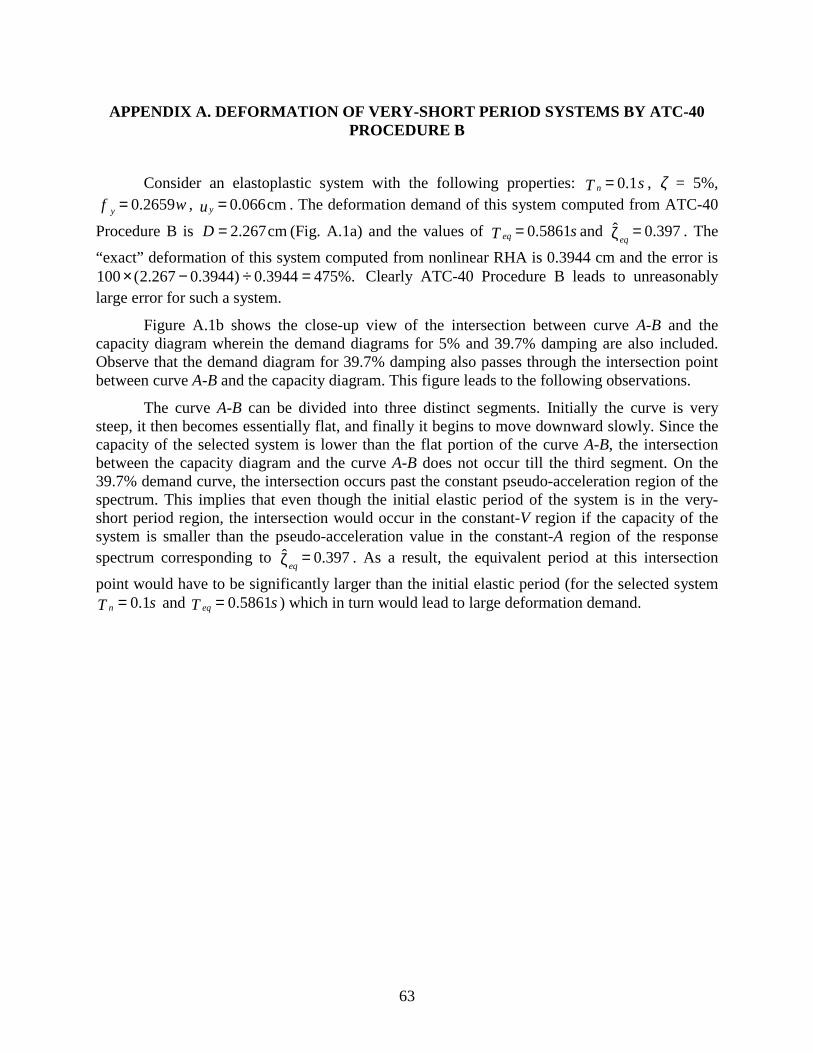
63

APPENDIX A. DEFORMATION OF VERY-SHORT PERIOD SYSTEMS BY ATC-40PROCEDURE B

Consider an elastoplastic system with the following properties: sTn 1.0= , ζ = 5%,wf y 2659.0= , cm066.0=uy . The deformation demand of this system computed from ATC-40

Procedure B is cm267.2=D (Fig. A.1a) and the values of sTeq 5861.0= and 397.0ˆ =ζeq. The

“exact” deformation of this system computed from nonlinear RHA is 0.3944 cm and the error is%.4753944.0)3944.0267.2(100 =÷−× Clearly ATC-40 Procedure B leads to unreasonably

large error for such a system.

Figure A.1b shows the close-up view of the intersection between curve A-B and thecapacity diagram wherein the demand diagrams for 5% and 39.7% damping are also included.Observe that the demand diagram for 39.7% damping also passes through the intersection pointbetween curve A-B and the capacity diagram. This figure leads to the following observations.

The curve A-B can be divided into three distinct segments. Initially the curve is verysteep, it then becomes essentially flat, and finally it begins to move downward slowly. Since thecapacity of the selected system is lower than the flat portion of the curve A-B, the intersectionbetween the capacity diagram and the curve A-B does not occur till the third segment. On the39.7% demand curve, the intersection occurs past the constant pseudo-acceleration region of thespectrum. This implies that even though the initial elastic period of the system is in the very-short period region, the intersection would occur in the constant-V region if the capacity of thesystem is smaller than the pseudo-acceleration value in the constant-A region of the responsespectrum corresponding to 397.0ˆ =ζeq

. As a result, the equivalent period at this intersection

point would have to be significantly larger than the initial elastic period (for the selected systemsTn 1.0= and sTeq 5861.0= ) which in turn would lead to large deformation demand.

64

0 10 20 30 40 500

0.2

0.4

0.6

0.8

1

D, cm

A, g

0.5 s 1 s

2 s

5 s

10 s

5% Demand DiagramA

B(2.267,0.2659)

(a)

0 1 2 3 4 50

0.2

0.4

0.6

0.8

1

D, cm

A, g

0.1 s 0.2 s

0.5 s

1 s

2 s

Capacity Diagram

5% Demand Diagram

39.7% Demand Diagram

A

B(2.267,0.2659)

(b)

Figure A.1. ATC-40 Procedure B applied to a system with Tn = 0.1s and Ay = 0.2659 g: (a)deformation demand; and (b) close-up view near the intersection between the demand andcapacity diagrams.

65

APPENDIX B: EXAMPLES USING TR ny −− µ EQUATIONS

SYSTEM 1

Consider an elastoplastic system with the following properties: sTn 5.0= , ζ = 5%,

gwfAy y5995.0=÷= . The pseudo-acceleration for linear-elastic system with sTn 5.0= , ζ = 5%

is gA 7062.2= . For this system, ( ) gATuD ynyy ××π== 2 2 ( ) 9805995.05.02 2 ××π= = 3.7202

cm and .51.45995.07062.2 =÷=Ry

Newmark-Hall Equation (Eq. 16)

The periods corresponding to various regions of the Newmark-Hall design spectrum aresTa 33/1= , sTb 125.0= , and sTc 6634.0= ; Tc' is unknown at this time because it depends on

µ that is yet to be determined. Since Tc' is unknown, it is not clear which equation — the third or

the fourth in Eq. (16) — should be used to determine µ. Assuming that TTT cnb '<< , gives

( ) ( ) 67.10251.4121 22 =÷+=÷+=µ Ry . For this value of µ, µ−µ= 12' TT cc

2804.067.10167.1026634.0 =−×= s. Clearly the assumption that TTT cnb '<< is not correct.Therefore, we must use the available equation for TTT cnc <<' , which gives TTR ncy ÷×=µ

99.55.06634.051.4 =÷×= . For this value of µ, 99.5199.526634.0' −×=Tc = 0.3674 s andthe assumption that TTT cnb '<< is valid. The deformation demand 7202.399.5 ×=D = 22.29cm.

Krawinkler-Nassar Equation (Eq. 19)

For elastoplastic force-deformation behavior, a=1 and b=0.42. Then( ) 1733.15.042.05.015.0 =÷++÷=c (Eq. 18) and ( ) ( )151.41733.111 1733.1 −×÷+=µ = 5.14.

The deformation demand 7202.314.5 ×=D = 19.11 cm.

Vidic-Fajfar-Fischinger Equation (Eq. 22)

Since µ is unknown at this time, To (Eq. 21) can not be determined at this time. Assumethat sTT co 6634.0== (Fajfar 1998), TsT on <= 5.0 . The first of the two equations in Eq. (22)

then gives ( )( )[ ] 69.4151.45.06634.074.01 053.1 =−×+=µ . The deformation demand =D7202.369.4 × = 17.43 cm.

SYSTEM 2



66

is gA 7062.2= . For this system, ( ) gATuD ynyy ××π== 2 2 ( ) 9808992.05.02 2 ××π= = 5.5803

cm and .01.38992.07062.2 =÷=Ry


Assuming that TTT cnb '<< , gives ( ) 03.5201.31 2 =÷+=µ . For this value of µ, Tc' =

3970.003.5/103.526634.0 =−×× s. Clearly the assumption that TTT cnb '<< is not correct.Therefore, we must use the available equation for TTT cnc <<' , which gives µ

99.35.06634.001.3 =÷×= . For this value of µ, 99.3199.326634.0' −×=Tc = 0.4393 s andthe assumption that TTT cnb '<< is valid. The deformation demand 5803.599.3 ×=D = 22.29cm.





Assuming that sTT co 6634.0== and using the first of the two equations in Eq. (22),

gives ( )( )[ ] 05.3101.35.06634.074.01 053.1 =−×+=µ . The deformation demand=D 5803.505.3 × = 17.02 cm.

SYSTEM 3



is gA 7062.2= . For this system, =Dy ( ) 9805624.15.02 2 ××π = 9.6962 cm and

.73.15624.17062.2 =÷=Ry


Assuming that TTT cnb '<< , gives ( ) 0.2273.11 2 =÷+=µ . For this value of µ, Tc' =

5745.00.2/10.226634.0 =−×× s and the assumption that TTT cnb '<< is valid. Thedeformation demand 6962.90.2 ×=D = 19.39 cm.




67


Assuming that sTT co 6634.0== and using the first of the two equations in Eq. (22),

gives ( )( )[ ] 71.1173.15.06634.074.01 053.1 =−×+=µ . The deformation demand=D 6962.971.1 × = 16.54 cm.

SYSTEMS 4 TO 6

Consider an elastoplastic systems with the following properties: sTn 1= , ζ = 5%,gggAy 8992.0and,4496.0,2997.0= for Systems 4, 5, and 6, respectively. The pseudo-

acceleration for linear-elastic system with sTn 1= , ζ = 5% is gA 7984.1= . For these system,

Dy = 7.4403 cm, 11.160 cm, and 22.321 cm, and corresponding values of Ry = 6, 4, and 2.


For TT cn > , Ry=µ = 6 for System 4, 4 for System 5, and 2 for System 6 which gives

DD y×µ= = 44.64 cm for all these examples.


For elastoplastic force-deformation behavior, a=1 and b=0.42. Then( ) 92.00.142.00.110.1 =÷++÷=c (Eq. 18). The values of µ for the three Systems are 5.56,

3.80, and 1.97 which give deformation demand D = 41.37 cm, 42.46 cm, and 43.97 cm.


For TT on > , values of µ for the three Systems are 4.97, 3.32, and 1.73 which givedeformation demand =D 36.94 cm, 37.0 cm, and 38.58 cm.

pacific earthquake engineering research...

Documents