pacific earthquake engineering research...

PACIFIC EARTHQUAKE ENGINEERING RESEARCH CENTER

Evaluation of Collapse and Non-Collapse of ParallelBridges Affected by Liquefaction and Lateral

Spreading

Benjamin Turner

Scott J. Brandenberg

Jonathan P. Stewart

Department of Civil and Environmental Engineering University of California, Los Angeles

PEER 2014/10AUGUST 2014

Disclaimer

The opinions, findings, and conclusions or recommendations expressed in this publication are those of the author(s) and do not necessarily reflect the views of the study sponsor(s) or the Pacific Earthquake Engineering Research Center.

Evaluation of Collapse and Non-Collapse of Parallel Bridges Affected by Liquefaction and Lateral

Spreading

Benjamin Turner

Scott J. Brandenberg

Jonathan P. Stewart

Department of Civil and Environmental Engineering University of California, Los Angeles

PEER Report 2014/10 Pacific Earthquake Engineering Research Center

Headquarters at the University of California, Berkeley

August 2014

iii

ABSTRACT

The Pacific Earthquake Engineering Research Center and the California Department of Transportation have recently developed design guidelines for computing foundation demands during lateral spreading using equivalent static analysis (ESA) procedures. In this study, ESA procedures are applied to two parallel bridges that were damaged during the 2010 M 7.2 El Mayor-Cucapah earthquake in Baja California, Mexico. The bridges are both located approximately 15 km from the surface rupture of the fault on soft alluvial soil site conditions. Estimated median ground motions in the area in the absence of liquefaction triggering are peak ground accelerations = 0.27g and peak ground velocity = 38 cm/sec (RotD50 components). The bridges are structurally similar and both are supported on deep foundations, yet they performed differently during the earthquake. A span of the pile-supported railroad bridge collapsed, whereas the drilled-shaft-supported highway bridge suffered only moderate damage and remained in service following the earthquake. The ESA procedures applied to the structures using a consistent and repeatable framework for developing input parameters captured both the collapse of the railroad bridge and the performance of the highway bridge. Discussion is provided on selection of the geotechnical and structural modeling parameters as well as combining inertial demands with kinematic demands from lateral spreading.

v

ACKNOWLEDGMENTS

This project was sponsored by the Pacific Earthquake Engineering Research Center’s (PEER's) Program of Applied Earthquake Engineering Research of Lifelines Systems supported by the California Department of Transportation (Caltrans) and the Pacific Gas and Electric Company. Any opinions, findings, and conclusions or recommendations expressed in this material are those of the authors and do not necessarily reflect those of the sponsors.

Members of the agency responsible for Mexican highways and communication infrastructure, SCT, provided valuable information and site access without which this project would not have been possible. We are also grateful for the assistance of Mr. Raúl Flores Berrones from the Instituto Mexicano de Tecnología del Agua for coordinating communication with SCT and the Mexican federal permitting agencies. We would also like to thank Enrique Hernandez Quinto and Ramón Pérez Alcalá from SCT for helping coordinate site access and explaining the history of the highway bridge.

We would like to thank Alberto Salamanca, Bob Nigbor, and Chris Krage for helping with the field testing. Alberto's Spanish fluency and charm proved particularly useful when the drive shaft on the hydraulic pump for the CPT rig cracked; he found a group of local mechanics to weld the shaft so we could leave the site before dark. We are grateful to Bill and Kathy Brandenberg for allowing us to stay in their home in Calexico during the field testing.

We are grateful for the opportunity to work with Tom Shantz of Caltrans for the duration of this project. We would also like to acknowledge the support of TRC Software in providing a license of XTRACT for moment-curvature analysis.

vii

CONTENTS

ABSTRACT .................................................................................................................................. iii

ACKNOWLEDGMENTS .............................................................................................................v

CONTENTS................................................................................................................................. vii

LIST OF FIGURES ..................................................................................................................... ix

LIST OF TABLES ..................................................................................................................... xiii

1 INTRODUCTION..............................................................................................................1

2 SITE DESCRIPTION AND INVESTIGATION ............................................................3

2.1 Regional and Local Geology .................................................................................3

2.2 Site Topography and Surface Conditions ............................................................5

2.3 Subsurface Conditions ...........................................................................................8

2.3.1 Previous Subsurface Investigations by Others .............................................8

2.3.2 Current Subsurface Investigation .................................................................9

2.3.3 Interpretation of Vs Profile .........................................................................12

2.4 Bridge Details .......................................................................................................15

2.4.1 Highway Bridge (HWB) ............................................................................15

2.4.2 Railroad Bridge (RRB) ..............................................................................19

2.5 April 4, 2010, M 7.2 El Mayor-Cucapah Earthquake ......................................19

2.6 Observed Damage ................................................................................................22

2.6.1 Ground Deformation ..................................................................................22

2.6.2 Structural Damage .....................................................................................24

3 ANALYSIS .......................................................................................................................27

3.1 Soil Properties ......................................................................................................29

3.2 Lateral Spreading Displacement ........................................................................35

3.3 Modeling of Structural Elements .......................................................................37

3.3.1 Moment-Curvature Analysis ......................................................................40

3.3.2 Elastomeric Bearings and Shear Tabs ........................................................42

3.4 Inertial Loads from Superstructure ...................................................................45

3.4.1 Spectral Displacement Method ..................................................................46

viii

3.4.2 Inertial Force Method ................................................................................47

3.5 Opensees Finite-Element Analysis ......................................................................49

3.6 Results ...................................................................................................................50

3.6.1 Response of Highway Bridge to Lateral Loading ......................................50

3.6.2 Response of Railroad Bridge .....................................................................52

3.6.3 Comparison of Combined Kinematic and Inertial Demand Methods......................................................................................................58

3.6.4 Settlement of Highway Bridge Bent 6 .......................................................61

4 CONCLUSIONS ..............................................................................................................65

REFERENCES .............................................................................................................................67

APPENDIX A: SUBSURFACE INVESTIGATIONS .....................................................71

APPENDIX B: LABORATORY TEST RESULTS ........................................................77

APPENDIX A: SAMPLE CALCULATIONS ..................................................................81

ix

LIST OF FIGURES

Figure 2.1 Regional map and key geologic features. Fault rupture zones after GEER [2010]; Cerro Prieto and Imperial Faults after Pacheco et al. [2006]. Google Earth base image. ........................................................................................4

Figure 2.2 View of site looking west across the Río Colorado from atop the east river bank. People standing near the river are adjacent to the railroad bridge span that collapsed during the 2010 El Mayor-Cucapah earthquake as a result of lateral spreading; steel columns to support temporary replacement trestle are visible (photo by B. Turner, January 2013). ...........................................6

Figure 2.3 Site plan showing locations of CPT, seismic survey lines, and sample collections from October 2013 site investigation and previous investigations. Mapped lateral spreading features and structural damage after GEER [2010]. Google Earth base image. ........................................................7

Figure 2.4 Cross section showing eastern spans of the highway bridge along with penetration resistances from previous and current studies. Location of cross section depicted in Figure 2.3. ......................................................................10

Figure 2.5 S- and P-wave velocity profiles and dispersion curves for Seismic Line 2 (location shown in Figure 2.3). ..............................................................................12

Figure 2.6 CPT-2 tip resistance, inferred shear-wave velocity profile, and dispersion curves used to fit parameters in Equation (2.1). ....................................................14

Figure 2.7 Profiles of shear wave velocity estimated at CPT test sites using Equation (2.1) with 0 = 0.5, 1 = 0.58, and 2 = 0.35. .....................................................14

Figure 2.8 Bent 1 of highway bridge showing shear tabs extending from transverse diaphragm into bent cap (top) and Bent 3 with no shear tabs (bottom) (photos B. Turner, 2013). .... ..................................................................................16

Figure 2.9 Cross section of highway bridge [SCT personal communication 2013]. ..............17

Figure 2.10 Construction of highway bridge foundations via casing and air lift method, circa 1999 (photo courtesy Ramón Pérez Alcalá, SCT). .......................................18

Figure 2.11 USGS Shakemap for PGA. Contours show Shakemap estimated PGA in %g based on GMPE estimates (not constrained by recordings south of the U.S.Mexico border). Measured PGA shown for SMA recording stations nearest the San Felipito Bridges. Adapted from USGS Shakemap [2010]. ...........21

Figure 2.12 Acceleration response spectra for strong-motion recording stations within 100 km of the fault rupture (Rjb) during the El Mayor-Cucapah earthquake along with predictions at San Felipito Bridges site. Data from PEER NGA-West2 Database Flatfile [PEER 2013]. ........................................................22

Figure 2.13 Approximately 3050 cm of apparent relative vertical displacement between the ground and river-side of columns at Bent 6 of the highway bridge. Apparent relative vertical displacement on the upslope side is about 10 to 15 cm (photo by J. Gingery, Kleinfelder/UCSD, 2011). ....................23

x

Figure 2.14 (a) Railroad bridge Bent 5 translated due to lateral spreading demand, causing an unseating collapse; arrow shows direction of movement (photo by D. Murbach, City of San Diego, 2011); and (b): flexural cracking at base of highway bridge Bent 5 extended-shaft column. Note that these two bents are adjacent to each other (photo B. Turner, 2013).. ....................................25

Figure 3.1 Numerical models of (a) highway bridge Bent 5 lateral analysis, (b)

railroad bridge Bent 5 lateral analysis, and (c) highway bridge Bent 6 axial analysis. ..................................................................................................................27

Figure 3.2 Cross section showing eastern spans of highway bridge and computed profiles of factor of safety against liquefaction and lateral spreading displacement. .........................................................................................................31

Figure 3.3 Profiles of cone tip resistance and estimated factor of safety against liquefaction, shear strain, lateral spreading displacement index, and lateral spreading displacement for CPT-1 data during the El Mayor-Cucapah earthquake. .............................................................................................................36

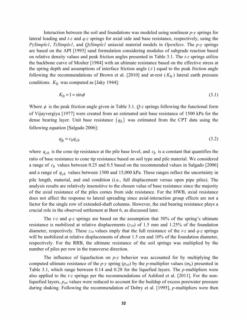
Figure 3.4 Estimated surface free-field lateral spreading (LD) displacement versus distance from free face (river bank) based on CPT-1, CPT-2, and CPT-3 profiles using the Zhang et al. [2004] approach. Decreasing LD with increasing distance appear to fit a linear (shown) or hyperbolic decay trend. ......................................................................................................................37

Figure 3.5 Highway bridge extended shaft column structural details. All dimensions in centimeters. Adapted from 1998 bridge construction plans [SCT, personal communication, 2013].............................................................................38

Figure 3.6 Railroad bridge member geometry and foundation group configurations considered for analysis. Clear edge spacing for all pile configurations is 0.4 m as shown for the 4×5 group. Refer to Table 3.10 for pile spacing and details. ....................................................................................................................38

Figure 3.7 Moment-curvature behavior for highway bridge 1.2-m diameter reinforced-concrete extended-shaft columns with zero axial load and corresponding bilinear model implemented in OpenSees. .....................................42

Figure 3.8 Highway bridge shear tab detail (top) and spring definitions used to model connection between superstructure and bent cap (bottom). ...................................44

Figure 3.9 Formulation of rotational stiffness of railroad bridge deck spans transferring load to column through elastomeric bearings. ...................................44

Figure 3.10 (a) Caltrans [2013a] force-based method for estimating top-of-foundation-level inertial shear and moment demands (VToF and MToF), and (b) spectral-displacement-based method after Ashford et al. [2011]. .......................................46

Figure 3.11 Moments resulting from lateral spreading and superstructure inertial demand. ..................................................................................................................49

xi

Figure 3.12 Highway bridge Bent 5 predicted response under imposed lateral spreading displacement demand of 1.0 m combined with superstructure inertia demand, represented as liquefaction-compatible spectral displacement demand, in opposite direction. .........................................................51

Figure 3.13 Maximum bending moment as a function of free-field lateral spreading displacement; this does not include inertial demands. ...........................................52

Figure 3.14 Railroad bridge Bent 5 analysis results showing collapse for a 4×5 group of 30-cm diameter reinforced concrete piles under imposed lateral spreading displacement demand of 1.0 m. Includes superstructure inertial demand, represented as liquefaction-compatible spectral displacement, in opposite direction from lateral spreading. Predicted column rotation ≈ 0.3°. Note the horizontal scale is exaggerated. ...............................................................53

Figure 3.15 Predicted response for railroad bridge Bent 5 with a 4×5 group of 30-cm reinforced concrete piles under imposed surface lateral spreading displacement (LD) of 1, 2, 3, and 4 m. Superstructure inertial demand, represented as liquefaction-compatible spectral displacement, is imposed in opposite direction from lateral spreading. Discontinuity in moment profile at pile-to-pile-cap connection occurs because the axial force in each pile row times its eccentricity from the pile cap centroid also contributes to moment resistance. ..........................................................................54

Figure 3.16 Results of parametric studies of railroad bridge Bent 5 foundation parameters under imposed lateral spreading demand of 1 m. Case numbers refer to Table 3.10. .................................................................................................57

Figure 3.17 Results of displacement- and force-based methods for combining superstructure inertial demands with 1-m of lateral spreading demand for highway bridges. Displacement-based approach provides best match to observed behavior. .................................................................................................59

Figure 3.18 Profiles of axial load (including downdrag) and axial resistance for highway bridge Bent 6 based on data from CPT-1 and CPT-2: (a): no liquefaction at tip—load carrying capacity is sufficient; and (b): loose layer at the depth of the foundation tip is liquefied, axial load exceeds the load carrying capacity of the foundation, resulting in bearing capacity failure and vertical settlement. ...............................................................................63

xiii

LIST OF TABLES

Table 3.1 Estimated soil properties for Bent 5 lateral spreading analyses. ...........................30

Table 3.2 Non-liquefied crust load-transfer parameters. .......................................................34

Table 3.3 Concrete (unconfined) properties. .........................................................................39

Table 3.4 Steel properties.......................................................................................................39

Table 3.5 Elastomeric bearing properties. .............................................................................39

Table 3.6 Timber (piles) properties. .......................................................................................39

Table 3.7 Highway bridge member properties. ......................................................................40

Table 3.8 Railroad bridge member properties. ......................................................................40

Table 3.9 Liquefaction-compatible foundation-level superstructure inertial demands for modified force-based analysis method. ............................................................49

Table 3.10 Summary of railroad bridge pile configurations analyzed. ....................................55

1

1 Introduction

The 2010 M 7.2 El Mayor-Cucapah (EMC) earthquake triggered liquefaction-induced lateral spreading in the vicinity of two bridges (highway and railroad) that cross the Colorado River in Baja California, Mexico. The bridges exhibited significantly different performance levels, despite being separated by only a few meters and both bridges being supported on deep foundations. The railroad bridge (RRB) suffered unseating collapse of one span and near collapse of another span, while the highway bridge (HWB) suffered moderate repairable damage without collapsing.

Since the soil conditions and imposed lateral spreading demands were essentially equivalent for the two bridges, this case study provides an excellent opportunity to validate recently-proposed equivalent-static analysis (ESA) procedures [Ashford et al. 2011; Caltrans 2013a] for analyzing bridge foundations subjected to lateral spreading. The objectives of this study were to apply the recommended ESA procedures to the two bridges and compare the predicted behavior to the performance that was observed following the EMC earthquake. Design procedures are often validated against failure case studies, but validation against cases of moderate to good performance is less common. The ability of a single method to predict the full range of possible performance levels indicates that it is a particularly robust tool that will be useful in practice.

An alternative to the ESA procedure for lateral spreading is to perform nonlinear dynamic numerical analyses where the soil and structure are modeled using two- or three-dimensional continuum elements, and input ground motions are provided that exhibit appropriate levels of spatial variability. Although this method can capture features of behavior neglected by ESA, dynamic methods can be costly and time-consuming to implement, require advanced user-expertise, and are limited in accuracy by the user’s ability to adequately estimate the parameters needed to define the material constitutive models. For routine design, this approach is not practical. Hence, the ESA procedure is a useful design tool as long as its predictive capabilities are properly validated. The ESA procedure can also be used to check the results of more advanced analyses when such analyses are justified by the nature of the project.

This report presents an overview of the San Felipito Bridges site and observed damage following the EMC earthquake, the geotechnical and structural modeling parameters used in our analyses, and the findings of our analyses of system performance.

3

2 Site Description and Investigation

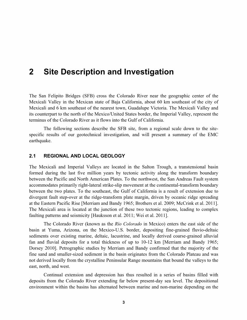
The San Felipito Bridges (SFB) cross the Colorado River near the geographic center of the Mexicali Valley in the Mexican state of Baja California, about 60 km southeast of the city of Mexicali and 6 km southeast of the nearest town, Guadalupe Victoria. The Mexicali Valley and its counterpart to the north of the Mexico/United States border, the Imperial Valley, represent the terminus of the Colorado River as it flows into the Gulf of California.

The following sections describe the SFB site, from a regional scale down to the site-specific results of our geotechnical investigation, and will present a summary of the EMC earthquake.

2.1 REGIONAL AND LOCAL GEOLOGY

The Mexicali and Imperial Valleys are located in the Salton Trough, a transtensional basin formed during the last five million years by tectonic activity along the transform boundary between the Pacific and North American Plates. To the northwest, the San Andreas Fault system accommodates primarily right-lateral strike-slip movement at the continental-transform boundary between the two plates. To the southeast, the Gulf of California is a result of extension due to divergent fault step-over at the ridge-transform plate margin, driven by oceanic ridge spreading at the Eastern Pacific Rise [Merriam and Bandy 1965; Brothers et al. 2009; McCrink et al. 2011]. The Mexicali area is located at the junction of these two tectonic regions, leading to complex faulting patterns and seismicity [Hauksson et al. 2011; Wei et al. 2011].

The Colorado River (known as the Río Colorado in Mexico) enters the east side of the basin at Yuma, Arizona, on the Mexico-U.S. border, depositing fine-grained fluvio-deltaic sediments over existing marine, deltaic, lacustrine, and locally derived coarse-grained alluvial fan and fluvial deposits for a total thickness of up to 10-12 km [Merriam and Bandy 1965; Dorsey 2010]. Petrographic studies by Merriam and Bandy confirmed that the majority of the fine sand and smaller-sized sediment in the basin originates from the Colorado Plateau and was not derived locally from the crystalline Peninsular Range mountains that bound the valleys to the east, north, and west.

Continual extension and depression has thus resulted in a series of basins filled with deposits from the Colorado River extending far below present-day sea level. The depositional environment within the basins has alternated between marine and non-marine depending on the

4

contemporary topography during deposition. Periodically, the Colorado River has terminated as a series of distributaries and shallow freshwater lakes that do not reach the Gulf of California, similar to the present configuration, although currently this phenomenon is exacerbated by human withdrawal of the majority of the river’s flow for agriculture and domestic consumption. Resulting lacustrine deposits of silt and clay can thus be found throughout the region. Flood overbank deposits are also responsible for fine-grained sediment in the area, particularly in the Imperial Valley as a result of floods of the river extending north of its usual course [Merriam and Bandy 1965; Dibblee 1984; Pacheco et al. 2006; Dorsey 2010].

Several faults cross the region as shown in Figure 2.1, primarily accommodating strike-slip movement in the northwest-southeast direction in combination with smaller oblique normal faults accommodating extension at the divergent step-over zones. The major plate boundary faults in the region are, from north to south, the San Andreas fault, the Imperial fault, and the Cerro Prieto fault. The EMC earthquake occurred as a sequence of ruptures along a series of faults considered to be west of the active plate boundary, including the Pescadores, Borrego, and previously unknown Indiviso faults [GEER 2010; Hauksson 2011].

Figure 2.1 Regional map and key geologic features. Fault rupture zones after

GEER [2010]; Cerro Prieto and Imperial Faults after Pacheco et al. [2006]. Google Earth base image.

5

Pacheco et al. [2006] estimated the average depth to crystalline bedrock in the central and eastern Mexicali Valley to be about 4 km using exploratory well data and geophysical methods. Basin depth further west of the Cerro Prieto fault has not been directly measured but is estimated to be significantly deeper than 4 km [Dorsey 2010]. Sediment depth has not been measured directly at the SFB site, but the studies by Pacheco et al. as well as others by the Mexican Federal Electricity Commission in support of the Cerro Prieto Geothermal Field [Davenport et al. 1981] indicate that unconsolidated (in the geologic sense) Quaternary sediments in the region vary in thickness between approximately 500 and 2500 m. Late Miocene and Pliocene sediments below this depth are mostly consolidated and in places have been subjected to low-grade metamorphism.

2.2 SITE TOPOGRAPHY AND SURFACE CONDITIONS

Nearly-level agricultural fields surround the area adjacent to the river, as can be seen in the background of Figure 2.2. Approach embankments that maintain the grade of the road at the elevation of the surrounding land are sufficient to provide about ten meters of clearance between the base of the bridges and the river surface during average flow.

The bridges cross the river at a gentle meander that has caused the active channel to migrate to the west side of its flood plain, which is about 175 m wide as seen in Figure 2.3. In the vicinity of the SFB crossing, the active river channel is approximately 50 m wide during the low and average flows that appear to be predominant for most of the year based on vegetation patterns observed at the site. The active channel is incised about 24 m below the flood plain terraces by a steep bank on the west side, and a more gradual slope on the east side (approximately 1.5 horizontal to 1 vertical (1.5H:1V) and 3~5H:1V, respectively). The flood plain terraces extend for about 25 m west of the active channel and about 90 m east of the active channel until meeting slopes that lead up to the adjacent fields. These slopes are about 2-3H:1V on the west bank and more gradual on the east bank. Constructed fills surrounding the bridge abutments slope down to the flood plain terraces at approximately 1.5H:1V.

The average natural ground slope is steeper on the west side of the river than on the east side because the bend in the river results in higher flow velocity and thus more erosive energy on the west side, with corresponding low velocity and sediment deposition on the inside of the bend. This pattern of topography is typical at bends in rivers flowing through alluvial valleys, and the resulting differences in relative density on each side of the river can significantly affect the behavior during earthquakes as was observed at the SFB site.

The ground surface is barren under and immediately north and south of the bridges, but in general the area is characterized by thick growth of tamarisk and other semi-aquatic and terrestrial bushes, extending from the water’s edge to between about 20 and 150 m away from the active channel banks. Rip-rap armoring has been placed around the abutment fills to provide erosion protection, visible in Figure 2.2.

6

Figure 2.2 View of site looking west across the Río Colorado from atop the

east river bank. People standing near the river are adjacent to the railroad bridge span that collapsed during the 2010 El Mayor-Cucapah earthquake as a result of lateral spreading; steel columns to support temporary replacement trestle are visible (photo by B. Turner, January 2013).

7

Figure 2.3 Site plan showing locations of CPT, seismic survey lines, and sample collections from October 2013 site

investigation and previous investigations. Mapped lateral spreading features and structural damage after GEER [2010]. Google Earth base image.

8

2.3 SUBSURFACE CONDITIONS

Our characterization of the subsurface conditions is based on review of previous reports and other documents associated with the original design and construction of the highway bridge (HWB), borings performed after the El Mayor-Cucapah (EMC) earthquake in support of repair efforts, and additional subsurface tests we performed for this study. The results of each will be discussed in the following sections.

2.3.1 Previous Subsurface Investigations by Others

The Mexican highway authority, Secretaría de Comunicaciones y Transportes (SCT), provided us with a cross section of the HWB showing profiles of blowcounts for five borings performed during the original subsurface investigation for the bridge design in 1998 as well as blowcounts from a post-earthquake boring [SCT, personal communication, 2013]. The approximate locations of these borings are shown on Figure 2.3. The documents provided by SCT indicate that the original exploratory borings were advanced using hydro-jetting and sampled using a standard penetration test (SPT) split spoon sampler. The post-earthquake boring was observed by members of the GEER reconnaissance team to be advanced in a similar manner, notably without the use of casing or slurry [GEER 2010]. Other design documents that SCT provided us indicate that index tests were performed on the samples retrieved during the original investigation, but the results of these tests were not available.

In general, the stratigraphy indicated by the SCT cross section consists of about 6 to 10 m of loose silty sand that gradually increases in relative density with depth, overlying a very dense layer of silty sand that resulted in refusal blow counts. The soil profile is uniformly described on the SCT cross section as poorly graded, light brown, very loose to very dense silty sand. Of the six borings, three show penetration resistance gradually increasing with depth. The other three borings, including the post-earthquake boring, show erratic increases and decreases in penetration resistance in the upper 10 m, with SPT N-values above 25 immediately below the surface and refusal at depths as shallow as 5 m, interbedded with low N-value layers. Some of the high penetration resistances may have been caused by friction along the sampling rods due to caving of the borehole prior to, or during, driving of the sampler.

The SCT also provided us with a cross section of the railroad bridge (RRB) that shows three post-earthquake borings performed in June 2012 by Ferrocarril Mexicano (Ferromex), the owner of the railroad, along with a complete log for one of the borings, which is included in Appendix A [SCT, Personal communication, 2013]. The boring log does not indicate whether hydro-jetting or a different form of drilling was used. The SPT samples were taken, and results of index tests performed on the retrieved samples are included on the boring log.

The Ferromex boring log shows SPT N-values between about 12 and 20 in the upper 7 m, followed by a gradual increase in relative density to refusal over the next 5 m. The general trend of these blow counts with depth is reasonable, but the average values are unexpectedly high in the shallow soil given that liquefaction and resulting lateral spreading were severe enough to

9

cause collapse of the adjacent RRB span. We suspect that the unexpectedly high penetration resistance measured in these borings may be due to the “nonstandard” nature of the SPT tests that were performed, i.e., that the use of hydro-jetting the unsupported borehole, using a rope and cathead hammer system, unknown hammer efficiency, etc., may have resulted in field blow counts that do not correspond to typical U.S. energy standards of 6090% efficiency.

Groundwater encountered in each of the borings suggests that the surface of the groundwater table is relatively constant across the site at approximately the same elevation as the river surface. Given the primarily course-grained soil at the site and the lack of geologic structural features that could cause artesian pressures, this interpretation is reasonable.

2.3.2 Current Subsurface Investigation

As a result of the uncertain nature of the SPT N-values from the previous investigations, as well as a lack of available index test results and our need to characterize the subsurface as accurately as possible in order to complete our analyses, we opted to supplement the available information by performing additional subsurface explorations at the site consisting of in situ testing and laboratory testing of retrieved samples.

Our investigation, completed in October of 2013, consisted of cone penetration testing (CPT) with shear wave velocity and porewater pressure measurements, hand sampling of near-surface soil, and spectral analysis of surface waves (SASW) geophysical testing. The locations of each exploration are shown on Figure 2.3.

The CPT soundings were performed using the NEES@UCLA 20-ton truck-mounted Hogentogler rig, which is capable of pushing to a maximum cone tip resistance (qt) of approximately 30 MPa. Four CPT's were successfully advanced to depths between 4.5 and 16.5 m, and several more attempted tests were stopped by obstructions at shallow depths. The obstructions were likely rubble from the original bridge construction or post-earthquake repair efforts. Shear wave velocity (Vs) measurements were taken at the CPT-3 location.

Profiles of cone tip resistance are shown in the Figure 2.4 cross section, and detailed profiles of tip resistance and friction ratio are presented in Appendix A.

Minimum and maximum void ratio and grain size analysis tests were performed on a bulk sample collected at the surface from location TP-1 (shown in Figure 2.3) in general accordance with ASTM standards. Laboratory test results are presented in Appendix B. The sample was found to be a uniformly graded silty fine sand, and the fines fraction was non-plastic. The fines content of 45% is higher than expected for the deeper layers, and most likely because a large amount of silt is deposited on the ground surface by wind and the river on a regular basis. This is supported by the grain size analysis results on the railroad boring; see Appendix A.

10

Figure 2.4 Cross section showing eastern spans of the highway bridge along with penetration resistances from

previous and current studies. Location of cross section depicted in Figure 2.3.

20

10

0

0 20qt [MPa]

10

0

0 20qt [MPa]

10

0

0 20qt [MPa]

20

10

0

0 50N

20

10

0

0 50N20

10

0

0 50N

20

10

0

30

0 50N

Approx. ground surfaceat time of exploration;used for analysis

Note:Vertical scale exagerated x2.5

11

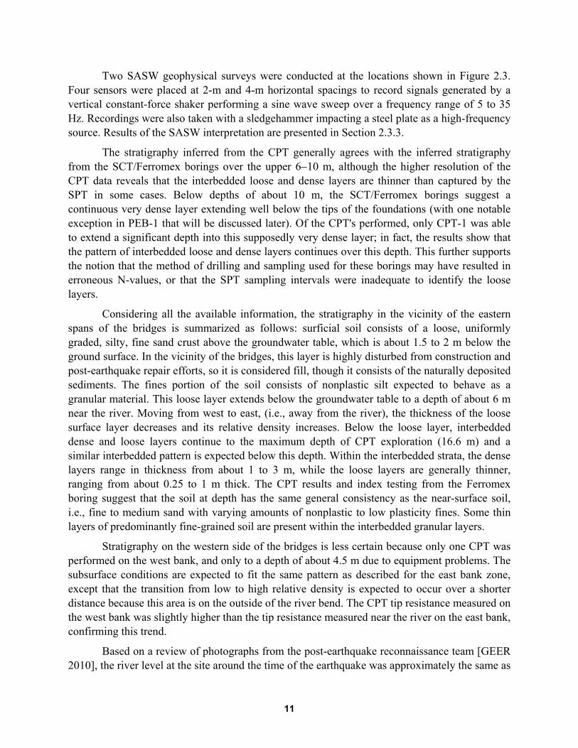
Two SASW geophysical surveys were conducted at the locations shown in Figure 2.3. Four sensors were placed at 2-m and 4-m horizontal spacings to record signals generated by a vertical constant-force shaker performing a sine wave sweep over a frequency range of 5 to 35 Hz. Recordings were also taken with a sledgehammer impacting a steel plate as a high-frequency source. Results of the SASW interpretation are presented in Section 2.3.3.

The stratigraphy inferred from the CPT generally agrees with the inferred stratigraphy from the SCT/Ferromex borings over the upper 610 m, although the higher resolution of the CPT data reveals that the interbedded loose and dense layers are thinner than captured by the SPT in some cases. Below depths of about 10 m, the SCT/Ferromex borings suggest a continuous very dense layer extending well below the tips of the foundations (with one notable exception in PEB-1 that will be discussed later). Of the CPT's performed, only CPT-1 was able to extend a significant depth into this supposedly very dense layer; in fact, the results show that the pattern of interbedded loose and dense layers continues over this depth. This further supports the notion that the method of drilling and sampling used for these borings may have resulted in erroneous N-values, or that the SPT sampling intervals were inadequate to identify the loose layers.

Considering all the available information, the stratigraphy in the vicinity of the eastern spans of the bridges is summarized as follows: surficial soil consists of a loose, uniformly graded, silty, fine sand crust above the groundwater table, which is about 1.5 to 2 m below the ground surface. In the vicinity of the bridges, this layer is highly disturbed from construction and post-earthquake repair efforts, so it is considered fill, though it consists of the naturally deposited sediments. The fines portion of the soil consists of nonplastic silt expected to behave as a granular material. This loose layer extends below the groundwater table to a depth of about 6 m near the river. Moving from west to east, (i.e., away from the river), the thickness of the loose surface layer decreases and its relative density increases. Below the loose layer, interbedded dense and loose layers continue to the maximum depth of CPT exploration (16.6 m) and a similar interbedded pattern is expected below this depth. Within the interbedded strata, the dense layers range in thickness from about 1 to 3 m, while the loose layers are generally thinner, ranging from about 0.25 to 1 m thick. The CPT results and index testing from the Ferromex boring suggest that the soil at depth has the same general consistency as the near-surface soil, i.e., fine to medium sand with varying amounts of nonplastic to low plasticity fines. Some thin layers of predominantly fine-grained soil are present within the interbedded granular layers.

Stratigraphy on the western side of the bridges is less certain because only one CPT was performed on the west bank, and only to a depth of about 4.5 m due to equipment problems. The subsurface conditions are expected to fit the same pattern as described for the east bank zone, except that the transition from low to high relative density is expected to occur over a shorter distance because this area is on the outside of the river bend. The CPT tip resistance measured on the west bank was slightly higher than the tip resistance measured near the river on the east bank, confirming this trend.

Based on a review of photographs from the post-earthquake reconnaissance team [GEER 2010], the river level at the site around the time of the earthquake was approximately the same as

12

the level during our October 2013 site investigation. This conveniently eliminates the need to re-interpret the CPT data for a different groundwater level.

2.3.3 Interpretation of Vs Profile

The shear-wave velocity profile was interpreted by combining the results of the SASW data with the CPT and SCPT measurements. This is a non-standard procedure that makes appropriate use of all of the available measurements. Typically, SASW inversion is performed based only on the measured Rayleigh wave dispersion curve. A problem with this procedure is that the inversion from the Rayleigh wave dispersion curve to a Vs profile is non-unique. For example, the velocity profiles in Figure 2.5 are associated with essentially identical first-mode Rayleigh wave dispersion curves, yet the velocity profiles clearly differ from each other. The dispersion curves in this case were computed using the finite element formulation developed by Lysmer [1970]. The vertical variations in the Vs profile could be important depending on the manner in which the velocity profile is utilized. For example, a one-dimensional site response analysis using the Profile 1 would likely differ significantly from the same analysis performed on Profile 3. Furthermore, Vs -based liquefaction triggering procedures could provide significantly different outcomes for the three profiles in Figure 2.5. However, a blind inversion of the first-mode Rayleigh wave dispersion curve (common practice in SASW) cannot possibly resolve the vertical variation of the velocity profile. For this reason, we have chosen to utilize the CPT tip resistance data to constrain the inversion of the dispersion curve.

Figure 2.5 S- and P-wave velocity profiles and dispersion curves for Seismic

Line 2 (location shown in Figure 2.3).

13

Correlations between Vs and penetration resistance have been formulated previously (e.g., Brandenberg et al. [2010] and DeJong et al. [2006]). The correlation tends to be rather poor, but provides an improvement in velocity estimates based on surface geology or topography alone. Much of the dispersion in the relation between Vs and penetration resistance arises from site-to-site variability rather than random variability within a specific site. For this reason, a site-specific calibration in which Vs and penetration resistance are independently measured can improve accuracy.

The approach adopted in this study is to utilize the functional relation between Vs, qt, and vertical effective stress v shown in Equation (2.1), and adjust the fitting parameters, 0 , 1 ,

and 2 , such that the resulting Vs profile produces a dispersion curve that matches the measured

curve. Note that the definition of the overburden scaling factor, n, is based on Robertson [2012]; see Appendix C. An overburden scaling term is required in the relation between Vs and tq

because these parameters are known to scale differently with overburden stress.

1 2

0

0.381 0.05 0.15 1.0

ns vt

c v a

V q

n I p

(2.1)

where Vs is in m/sec, tq is in kPa, v is vertical effective stress in kPa, ap is atmospheric

pressure (101.325 kPa), and cI is the soil behavior type index.

The CPT-2 sounding and dispersion curve measured for Seismic Line 2 were used in this study, and the following constants were found to provide a good fit as shown in Figure 2.6: 0 =

0.5, 1 = 0.58, and 2 = 0.35. This particular combination of CPT-2 and Seismic Line 2 were

selected because: (1) they are at similar distances from the river, and site conditions are known to depend on this distance; and (2) the soil directly below the HWB at the location of Seismic Line 1 is known to have been significantly reworked during post-earthquake construction to retrofit the bridge foundations. Therefore this soil does not represent site conditions outside of the bridge footprint.

14

Figure 2.6 CPT-2 tip resistance, inferred shear-wave velocity profile, and

dispersion curves used to fit parameters in Equation (2.1).

Utilizing the values determined for CPT-2 and Seismic Line 2, Vs profiles can be

computed at the location of other CPT test sites, as shown in Figure 2.7. Comparing CPT-1, 2, and 3, the velocity profile tends to stiffen with increasing distance from the river, which is consistent with the interpreted geology at the site and the trends in the penetration resistance tests. Comparing CPT-1 and CPT-4, which are similar distances from the river but on opposite banks, the west bank of the river tends to be stiffer than the east bank. This is also consistent with geological conditions since younger deposits exist on the east side of the river. Time-averaged shear wave velocity over the upper 30 m (Vs30) was estimated to range between approximately 180 and 230 m/sec for subsequent calculations.

Figure 2.7 Profiles of shear wave velocity estimated at CPT test sites using

Equation (2.1) with 0 = 0.5, 1 = 0.58, and 2 = 0.35.

15

2.4 BRIDGE DETAILS

The HWB and RRB both consist of precast-prestressed simply supported concrete spans on elastomeric bearings resting atop reinforced concrete bents supported on deep foundations. The bents of the HWB were designed to match the 20-m spacing of the RRB, with ten spans total for an overall length of 200 m. The primary difference between the two bridges is the size and number of foundations that support each bent, which will be described further in the following sections.

2.4.1 Highway Bridge (HWB)

The following structural details are primarily based on the bridge construction plans (1998) provided to the research team by SCT. The HWB was designed by a private engineering firm from Mexico City, Sigma Ingenieria Civil, S.A. de C.V.

Each of the bridge’s ten 20-m-long spans consists of seven precast-prestressed 1.15 m-deep I-shaped girders. Vertical post-tensioned diaphragms connect the ends of the girders in the transverse direction. Precast slab panels rest on the top flanges of adjacent girders, covered by a cast-in-place deck slab. The total deck width is about 11 m. Plain laminated elastomeric bearings transfer loads from the girders to 60-cm-wide concrete masonry plates atop the 1.6-m-wide bent caps, which are in turn supported on four extended-shaft columns.

At the bents between spans 34 and 78, as well as at the end supports at the abutments, the only connection between the girders/diaphragm and the bent cap is the elastomeric bearings. The bearings transfer load and allow for relative displacement and rotation between the superstructure and the substructures by compressing and deforming in shear. The deck slabs are separated by a polymer-filled joint at these locations to allow for thermal expansion and contraction.

At the remaining bents, including Bent 2 and Bent 5 that suffered flexural damage during the EMC earthquake, translation of the girders is restrained by anchorage via two rectangular shear tabs that extend from the base of the diaphragm into the bent cap, as shown in Figure 2.8. The anchorage tabs fit into a rectangular slot cast into the bent cap such that translation is restrained in both the longitudinal and transverse directions. A felt pad lines the joint between the anchorage tabs and the bent cap; no reinforcing bars form a positive connection between the two elements. A small amount of rotation is allowed at these connections, hence they are considered to be “pinned” as opposed to moment-resisting connections. It is assumed that the elastomeric bearings are intended to accommodate lateral deformation under service loads, while the anchorage tabs are meant to prevent unseating during extreme events. The end conditions of all ten spans are considered simply supported.

At each bent, four 1.2-m-diameter extended-shaft columns are continuous with four drilled shaft foundations of the same size and reinforcement detail. A transverse beam near the ground level joins the shafts at each bent with the exception of Bent 2, which has a larger pile cap. The foundations in the river extend to the deepest elevation, approximately 17 m below the

16

river surface elevation, as shown in Figure 2.4, while the foundations nearest the abutments and beneath the eastern spans where the river flows less frequently are shorter by 3 to 6 m. A cross section of the bridge adapted from the construction plans is shown in Figure 2.9.

Figure 2.8 Bent 1 of highway bridge showing shear tabs extending from

transverse diaphragm into bent cap (top) and Bent 3 with no shear tabs (bottom) (photos B. Turner, 2013).

17

Figure 2.9 Cross section of highway bridge [SCT personal communication 2013].

18

Design documents provided by SCT indicate that each shaft was designed to carry an allowable axial load of about 2100 kN. We estimated the axial dead load from the superstructure (girders, deck, and nonstructural components) to be about 1050 kN, which is consistent with a static factor of safety against axial failure of 2.0, although this does not consider the self-weight of the column. It is not known if the bridge was explicitly designed to resist loads resulting from liquefaction such as downdrag or lateral spreading, but the absence of any discussion of these subjects in the design documents suggests they were not considered.

During the October 2013 site investigation, Mr. Ramón Pérez Alcalá, an engineer for SCT who was responsible for overseeing construction of the bridge in 19981999, provided information on the methods used to construct the foundations. Temporary steel casing was advanced under its own weight, or using hydraulic jacks in stiff layers, while the spoils were removed by air lifting. Water was pumped from the river and maintained at or above ground level to keep a positive head within the hole. Concrete was placed using the tremie method after the reinforcing cages were in place. All the foundations were installed to the depths shown on the construction plans. A cold joint exists at the approximate ground surface elevation during construction since the columns were not ready to be constructed when the foundations were poured. Based on photographs provided by Mr. Alcalá, such e.g., Figure 2.10, the foundation reinforcing cages are lap spliced with the column reinforcement by approximately 3 to 4 m.

Figure 2.10 Construction of highway bridge foundations via casing and air lift

method, circa 1999 (photo courtesy Ramón Pérez Alcalá, SCT).

19

Mr. Alcalá also explained why Bent 2 has a pile cap not present at the other bents. A void related to a previous structure was encountered during construction of the foundations. Since a foundation passing through the void could not be relied upon, a fifth shaft was constructed south of the bridge and connected to the other foundations and columns via the pile cap.

Further information regarding the dimensions and mechanical properties of the bridge elements is provided in Section 3.3

2.4.2 Railroad Bridge (RRB)

The RRB, constructed in 1962 [EERI 2010], consists of a single track supported on three 1.2 m-deep I-shaped girders. The simply supported spans rest on plain elastomeric bearings atop oblong-shaped reinforced concrete pier walls that are most likely supported on driven pile foundations. No shear keys or other form of anchorage were observed to prevent an unseating failure if the elastomeric bearing capacity is exceeded. Simply supported concrete slab walkways parallel the track on each side. The research team was unable to obtain construction plans or design documents for the RRB.

Foundation details are unknown, but given the timeframe of construction, the fluvial environment, and the propensity of North American railroad companies to use driven pile foundations to this day (e.g.,, the post-earthquake repair of the RRB utilized driven steel piles), it is most likely that the pile caps are supported on driven pile foundations as opposed to drilled shafts. Because it is not known whether timber, concrete, or steel piles were used, we performed analyses considering all three materials over a range of sizes and group layouts; see Chapter 3.

In order to quantify the structural properties of the RRB for modeling purposes, direct measurements of the above-ground member geometry were taken during the October 2013 site investigation. The size of the pile cap was inferred from photographs taken by members of the GEER team [2010] during the repair efforts by Ferromex in which the soil above and around the pile cap had been excavated to facilitate installing new driven piles.

Given the date of construction, it is almost certain that the RRB foundations were not designed to resist the effects of liquefaction and lateral spreading.

2.5 APRIL 4, 2010, M 7.2 EL MAYOR-CUCAPAH EARTHQUAKE

The Mexicali and Imperial Valley region is known to be seismically active, with several major earthquakes occurring in recent history, including an estimated M 7.2 event in 1892 [Hough and Elliot 2004]. The EMC earthquake caused widespread damage to buildings, utilities, and transportation and agricultural infrastructure throughout the Mexicali and Imperial Valleys [GEER 2010; EERI 2010].

Rupture occurred mainly along the Pescadores and Borrego faults through the Sierra El Mayor mountain range northwest of the epicenter and the previously unknown Indiviso fault to the southeast, which was buried beneath sediments of the Colorado River delta prior to the

20

earthquake ([GEER 2010; USGS 2010; McCrink et al. 2011]. This series of faults represents the southern continuation of the Elsinore fault zone in Southern California. Fault offset was oblique with the primary component being strike-slip. Further details of the complex rupture propagation, which appears to have started along a short unnamed normal fault and then propagated north and south along the strike-slip faults, are provided in GEER [2010], Hauksson et al. [2011], and Wei et al. [2011].

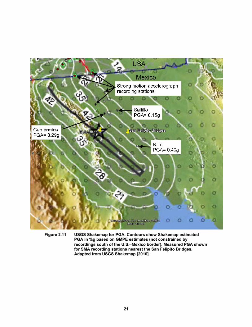
The SFB site is approximately 14.5 km east of the fault rupture zone (Rjb; note Rjb = Rrup for vertical strike-slip faults). The three nearest strong-motion recording stations are Riito, Saltillo, and Geotérmica, located approximately 12, 21, and 24 km from the SFB, respectively (see Figure 2.11). Peak ground accelerations (PGA) recorded at the three stations were 0.40, 0.15, and 0.29g, respectively. A weighted average based on distance of these three values yields a PGA of 0.29g for the SFB site, but this estimate fails to consider site effects and is clearly inaccurate due to the variability of the three recorded motions. Acceleration response spectra (RotD50) for strong-motion recording stations within 100 km of the fault rupture for the EMC earthquake are shown in Figure 2.12.

The USGS PGA Shakemap [USGS 2010] for the EMC earthquake estimates a PGA of about 0.32g for the SFB site, as shown in Figure 2.11. However, the Shakemap PGA values south of the U.S.Mexico border are based entirely on estimated ground motions using “standard seismological inferences and interpolation” and are not constrained by recorded motions [USGS 2014]. The nearest recording station to the SFB site used to generate the USGS Shakemap is approximately 50 km to the northwest; hence the estimated value is only approximate and does not consider local site effects.

In order to estimate PGA at the SFB site including site effects, we applied the procedures described by Kwak et al. [2012]. In this method, a Kriging (spatial interpolation) procedure is used to estimate the residual of the selected ground motion prediction equation (GMPE) at the location of interest considering the residuals at nearby recording stations and the event term. (The residual is the misfit between a recorded motion and the GMPE prediction for that location, and the event term is the average of the residuals for all recordings from the earthquake, essentially representing the average misfit of the GMPE to the recordings.) This procedure captures the event term directly and approximately accounts for region-specific path terms. Site effects are captured at the level of resolution of the site term in the GMPE (i.e., they are not site-specific, hence this does not correspond to a single-station sigma condition; e.g., Rodriguez-Marek et al., [2011]). We used this technique to estimate the residual at the SFB site (about -0.04 for PGA), and subsequently added it to the median predicted PGA from the BSSA 2014 GMPE [Boore et al. 2014] with appropriate site and distance parameters. The resulting estimated PGA range is 0.26 to 0.27g for estimated Vs30 values of 180 to 230 m/sec, respectively. The same procedure was repeated for spectral acceleration at periods corresponding to the estimated first mode periods of the SFB (determination of these values is discussed in Section 3.4). The estimated values of spectral acceleration are shown in Figure 2.12, including error bars that represent within-event aleatory uncertainty (± ). The predicted spectral accelerations plot

approximately in the middle of the range of the recorded spectra with Rjb less than 50 km.

21

Figure 2.11 USGS Shakemap for PGA. Contours show Shakemap estimated

PGA in %g based on GMPE estimates (not constrained by recordings south of the U.S.Mexico border). Measured PGA shown for SMA recording stations nearest the San Felipito Bridges. Adapted from USGS Shakemap [2010].

22

Figure 2.12 Acceleration response spectra for strong-motion recording stations

within 100 km of the fault rupture (Rjb) during the El Mayor-Cucapah earthquake along with predictions at San Felipito Bridges site. Data from PEER NGA-West2 Database Flatfile [PEER 2013].

2.6 OBSERVED DAMAGE

This section summarizes the observed ground failure and structural damage attributed to the EMC earthquake at the SFB site as documented by the GEER [2010] and EERI [2010] teams. Further details of the damage are available in the respective reconnaissance reports. The observed behavior was used as the basis for evaluating the predictive capability of the analyses described in Chapter 3.

2.6.1 Ground Deformation

Lateral spreading cracks were documented by the GEER team; see Figure 2.3. The maximum documented lateral spreading surface displacement, based on summing the width of cracks at the ground surface along a transect, was 4.6 m towards the east river bank about 60 m north of the bridges. Lateral spreading along the bridge alignment was reduced due to the restraining influence of the bridge foundations. However, this is not a traditional "pinning" effect (e.g., Martin et al. [2002]) because the out-of-plane width of the spreading deposit is very large relative to the bridge foundations; therefore, the resistance provided by the foundations is negligible compared to the inertial force of the displacing crust. (In contrast, the foundation resistance is significant for the case of a finite-width earth structure such as an embankment).

Sa

(g)

23

Thus a free-field ground displacement profile is needed for structural analysis, and the measurements 60 m north of the bridge are considered reasonable estimates of the free-field conditions.

Lateral spreading deformation was observed to be greater on the east bank of the river than the west bank, which is likely because the river currently flows along the western margin of its floodplain so the alluvial sediments on the east bank are looser and more susceptible to liquefaction. Similar deformation patterns at a river bend are documented by Robinson et al. [2012]. In general, lateral displacements were observed to decrease with increasing distance from the river, as well as in close proximity to the bridges.

At the HWB Bent 6, apparent vertical ground settlement of about 30 to 50 cm relative to the bridge columns was observed on the river-side of the columns; see Figure 2.13. The apparent relative vertical displacement on the upslope side of the columns was smaller, about 10 to 15 cm. These estimates of settlement are based on the assumption that the height of soil stuck on the sides of the columns (as shown in Figure 2.13) is representative of the ground level immediately preceding the earthquake; however, other explanations for the soil marks cannot be ruled out. The settlement was likely due to a combination of post-liquefaction reconsolidation of the liquefied soil layers and extension/shear strains associated with lateral spreading of the crust. As a result, there is no means for independently measuring the amount of vertical settlement that occurred due to reconsolidation alone.

Figure 2.13 Approximately 3050 cm of apparent relative vertical displacement

between the ground and river-side of columns at Bent 6 of the highway bridge. Apparent relative vertical displacement on the upslope side is about 10 to 15 cm (photo by J. Gingery, Kleinfelder/UCSD, 2011).

24

The Bent 6 columns themselves also settled about 50 cm as evidenced by vertical displacement in the bridge deck. Combined with the 3050 cm of apparent relative displacement between the ground and the river-side of the column, this indicates that the total ground settlement may have been as much as 0.81.0 m downslope of the columns, and about 0.6 m upslope of the columns.

2.6.2 Structural Damage

The bents of the RRB closest to the east and west river banks translated toward the river due to lateral spreading, which exceeded the lateral displacement capacity of the elastomeric bearings and led to unseating of the girders for a span on the eastern bank and near-collapse of a span on the west bank (Figure 2.14). The translation was observed to occur with relatively little corresponding pier rotation. The bridge deck also displaced in the transverse direction relative to the bents; although displacements in the longitudinal direction were greater. Ferromex erected steel trestles to replace the collapsed span and support the nearly collapsed span on the west bank.

Damage to the HWB was concentrated in discrete zones and was moderate overall. In contrast to the RRB, the HWB exhibited much better performance; it remained in operation immediately following the earthquake and required repair efforts that were completed with minimal disruption to traffic. The damage documented by the reconnaissance teams is summarized as follows:

Shear keys extending up from the ends of the bent caps intended to prevent unseating of the girders in the transverse direction were damaged, indicating that inertial demands in this direction were significant. Shear keys on the west abutment bent cap were damaged in a similar manner.

Flexural cracking was observed on the inward (river side) of the base of the columns of the bents on both sides of the river (Bent 2 and Bent 5), indicating horizontal movement of the foundations and pile cap towards the center of the river due to lateral spreading. Cracks on Bent 5 are shown in Error! Reference source not found.. The bridge deck showed minor cracking above these damaged bents.

Bent 6 settled vertically about 50 cm, which cracked the pavement immediately above the bent. SCT subsequently installed six additional 1.2-m diameter drilled shafts to a depth of 27.8 m around the perimeter of the existing Bent 6 foundations and connected the new and old foundations via a post-tensioned pile cap [SCT, personal communication, January 2013]. Post-earthquake boring 1 (PEB-1, shown in Figure 2.3) was performed adjacent to Bent 6 in support of the design effort for the additional foundations. The deck was subsequently re-leveled and the concrete masonry pads that support the elastomeric bearings were extended vertically to accommodate the height change.

25

We measured column rotations for the bridge bents on the east side of the river during the October 2013 site investigation. HWB Bent 5 columns were rotated between approximately 0.9° and 1.7° away from the river, i.e., the bottom of the column was displaced towards the river relative to the top of the column. The measured rotation was smallest for the column closest to the RRB and increased approximately linearly to the south, indicating that more lateral spreading demand was imposed on the south columns than the north. HWB Bent 6 columns were uniformly rotated about 1.1° away from the river. Rotations for Bents 7, 8, and 9 ranged between about 0.4° and 0.1°, with a clear trend of decreasing rotation with increasing distance from the river. The RRB Bent 5 column, which translated enough to cause unseating of one of the spans it supported, rotated about 0.4° away from the river and about 0.6° to the north; it was difficult to measure the rotation because the surface of the column was rough. The remaining RRB bents on the east side of the river had essentially zero measureable rotation.

(a) (b)

Figure 2.14 (a) Railroad bridge Bent 5 translated due to lateral spreading demand, causing an unseating collapse; arrow shows direction of movement. (photo by D. Murbach, City of San Diego, 2011); and (b) flexural cracking at base of highway bridge Bent 5 extended-shaft column. Note that these two bents are adjacent to each other (photo B. Turner, 2013).

Extended-Shaft Column

Transverse Diaphragm

Flexural Cracking

27

3 Analysis

In order to validate the equivalent static analysis (ESA) procedures recommended by Ashford et al. [2011] and Caltrans [2013a], the San Felipito Bridges (SFB) were analyzed as described in this chapter and the results compared to the observed behavior described in the previous chapter. Three separate analyses were performed as depicted in Figure 3.1:

Highway bridge (HWB) Bent 5 with imposed lateral spreading and inertial demands,

Railroad bridge (RRB) Bent 5 with imposed lateral spreading and inertial demands. We considered group configurations with two and four rows of piles in the bridge longitudinal direction as discussed in 3.6.2, and

HWB Bent 6 under axial downdrag loads.

The locations of Bents 5 and 6 are shown on the Figure 2.3 site plan and the cross sections in the previous chapter.

Figure 3.1 Numerical models of (a) highway bridge Bent 5 lateral analysis, (b)

railroad bridge Bent 5 lateral analysis, and (c) highway bridge Bent 6 axial analysis.

28

The project scope initially included analyzing HWB Bent 2 under lateral spreading demand. However, we were unable to perform site investigation at this location due to a malfunction of the CPT rig. Furthermore, the revelation that an additional foundation was installed here because of an underground void discovered during construction complicated the structural modeling.

A detailed treatment of the steps required to perform the ESA procedure is given by Ashford et al. [2011] and Caltrans [2013a] and will not be repeated here, however some of the calculations performed to quantify input parameters for the analyses are included in Appendix C. In summary, the methods provide a set of relatively simple tools that foundation engineers can use to estimate the engineering demand parameters (EDP) necessary to design bridge foundations in laterally spreading ground. The foundation design is intended to be performed in concert with the design of the superstructure in order to provide compatible behavior at the desired performance level.

The ESA procedure is performed using a two-dimensional static beam on nonlinear Winkler foundation (BNWF) approach. We performed the analyses for this project using the finite-element modeling platform OpenSees [McKenna 1997]. In theory, the analysis could be performed with any numerical analysis software that incorporates the BNWF approach and allows the user to impose a displacement profile to the free ends of the soil springs to simulate lateral spreading, and permits adequate consideration of important structural details. For example, the Caltrans [2013a] lateral spreading design guidelines describe how to perform the analysis using the finite-difference method program LPILE made by ENSOFT [Reese et al. 2005]. We opted to use OpenSees instead of LPILE because (1) it permits more detailed structural modeling (e.g., bearings between piers and girders, rotational stiffness at the top of the pier column, etc.), (2) we can model groups of piles (ENSOFT also makes GROUP, which permits analysis of pile groups), and (3) we do not own licenses of LPILE or GROUP, whereas OpenSees is freely available.

Since the HWB bents consist of four identical extended-shaft columns with approximately equal tributary loads, the analysis was performed for a single shaft, and the results are assumed to represent the behavior of all four shafts at the bent. The shafts form a single row in the bridge transverse direction, so group-interaction effects do not apply for lateral spreading loading in the bridge longitudinal direction. In contrast, the RRB bents consist of a single column supported on a pile cap that connects multiple rows of piles (we assume multiple rows of piles exist based on traditional construction methods). To accurately capture the foundation group-interaction effect (i.e., the overturning resistance provided by the axial load in each row of piles times its eccentricity from the pile cap centroid), the system was explicitly modeled with multiple rows of piles. Each row of piles for the RRB is represented by a single pile with a flexural rigidity (EI) equal to the EI of a single pile times the number of piles in the transverse row. The actual number of rows of piles and number of piles per row for the RRB is unknown; Section 3.6.2 includes discussion on how we dealt with this uncertainty in the analysis.

We chose to explicitly model the above-ground portions of the bridge bents up to the elastomeric bearings. An alternative that is often used when modeling using LPILE or GROUP is

29

to decouple the column demands from the foundation demands and impose the estimated column demands on the foundation for the BNWF analysis. However, explicitly modeling the columns is a superior approach because in many cases the lateral spreading demands are resisted by a combination of the foundation(s) and superstructure (i.e., the columns, girders, and deck segments), and knowing the demands at the base of columns a priori is often not possible. Furthermore, our knowledge of the damage to the bridges in this study is based primarily on post-earthquake observations of above-ground structural elements, namely cracking, rotation, and translation of columns. Since this damage was used as the basis for evaluating the accuracy of the predicted EDP, it was necessary to include the above-ground elements in the model.

The following sections document the input parameters used in the OpenSees models of the bridges followed by results of the analyses.

3.1 SOIL PROPERTIES

The CPT data were correlated to soil properties using the procedures described by Robertson [2012] and Idriss and Boulanger [2008]. Peak friction angle was estimated in a manner consistent with critical state soil mechanics with an assumed critical state friction angle of 32° for quartz sand [Bolton 1986]. Further details of the correlations are provided in Appendix C. Soil properties for each layer of the idealized soil profile used for the lateral spreading analyses are presented in Table 3.1.

Using the overburden-normalized penetration resistance profiles presented in Appendix A and the soil properties presented below, liquefaction susceptibility and triggering analyses were performed per the recommendations of Idriss and Boulanger [2006; 2008]. Soil layers with Ic less than 2.6 were assumed susceptible to liquefaction, which is supported by the laboratory tests we performed that showed that the fines fraction of the silty sand consisted of nonplastic silt. Groundwater depth was taken as 1.5 m below the ground surface.

Because lateral spreading demand acting on the bridges represents a liquefied soil condition, discretization of the soil profile into the idealized layers presented in Table 3.1 was based primarily on the results of the liquefaction triggering analysis. Correlated soil properties such as relative density and peak friction angle were then computed based on the average values estimated over the depth interval of each layer.

We performed analyses for the estimated PGA range of 0.17 to 0.41g to capture the uncertainty in Vs30 and the within-event aleatory uncertainty ( ) in the estimated shaking

intensity. Triggering of lateral spreading is dependent on the upper loose layer (layer 1 in Table 3.1) liquefying, which it is predicted to do for PGA values greater than about 0.15g. Hence, liquefaction and lateral spreading are predicted for the entire range of PGA values considered for this analysis (0.17 to 0.41g). The estimated lateral spreading displacement at the ground surface using the data from CPT-1 was 3.77 m for the median predicted PGA of 0.27g, with a range of 2.78 to 3.82 m for the median minus/plus one standard deviation PGA values of 0.17 and 0.41g, respectively. The predicted lateral spreading displacement saturates at values of PGA exceeding about 0.23g because maximum shear strains trend towards a limiting value for low factors of

30

safety against liquefaction (FSliq). We conclude from these results that lateral spreading demand is relatively insensitive to the range of PGA considered, and thus will use the median estimated PGA of 0.27g from this point forward.

Profiles of FSliq and estimated lateral spreading displacement using data from CPT-1 are shown in Figure 3.2 and are included alongside the CPT data profiles in Appendix A. Estimation of lateral spreading displacement is discussed in Section 3.2.

Table 3.1 Estimated soil properties for Bent 5 lateral spreading analyses.

Lay

er

Description Depth range

(m)

Unit wt.a

(kN/m3)

rD b

(%)

Peak friction anglec

60N d

Excess PWP ratioe

ru (%)

Fully--iquefied P-multiplierf

,p liqm

P-multiplier

pm

1 unsaturated

silty sand crust 0–1.5 17 55 35° 10 N/A N/A N/A

2 loose sand 1.5–6.5 18 42 35° 8 100 0.14 0.14

3 dense sand 6.5–8.4 18 77 40° 27 40 0.47 0.93

4 medium-dense

sand 8.4–11.2 18 54 37° 20 100 0.28 0.28

5 very dense

sand >11.2 19 82 41° 44 5 0.70 0.98

aBased on judgment. bBased on a weighted average of Idriss and Boulanger [2008], Zhang et al. [2004], and Kulhawy and Mayne [1990]; see Appendix C. cRobertson [2012] and Bolton [1986] dBased on correlation to qt and Ic per Robertson [2012]; see Appendix C. ePWP = porewater pressure; median prediction of correlation by Cetin and Bilge [2012] between shear strain and ru is shown. fBrandenberg [2005]

31

Figure 3.2 Cross section showing eastern spans of highway bridge and computed profiles of factor of safety against

liquefaction and lateral spreading displacement.

32

Interaction between the soil and foundations was modeled using nonlinear p-y springs for lateral loading and t-z and q-z springs for axial side and base resistance, respectively, using the PySimple1, TzSimple1, and QzSimple1 uniaxial material models in OpenSees. The p-y springs are based on the API [1993] sand formulation considering modulus of subgrade reaction based on relative density values and peak friction angles presented in Table 3.1. The t-z springs utilize the backbone curve of Mosher [1984] with an ultimate resistance based on the effective stress at the spring depth and assumptions of interface friction angle ( ) equal to the peak friction angle following the recommendations of Brown et al. [2010] and at-rest ( 0K ) lateral earth pressure

conditions. 0K was computed as [Jaky 1944]:

0 1 sinK (3.1)

Where is the peak friction angle given in Table 3.1. Q-z springs following the functional form

of Vijayvergiya [1977] were created from an estimated unit base resistance of 1500 kPa for the dense bearing layer. Unit base resistance bq was estimated from the CPT data using the

following equation [Salgado 2006]:

b cbq c qb (3.2)

where cbq is the cone tip resistance at the pile base level, and bc is a constant that quantifies the

ratio of base resistance to cone tip resistance based on soil type and pile material. We considered a range of bc values between 0.25 and 0.5 based on the recommended values in Salgado [2006]

and a range of cbq values between 1500 and 15,000 kPa. These ranges reflect the uncertainty in

pile length, material, and end condition (i.e., full displacement versus open pipe piles). The analysis results are relatively insensitive to the chosen value of base resistance since the majority of the axial resistance of the piles comes from side resistance. For the HWB, axial resistance does not affect the response to lateral spreading since axial-interaction group effects are not a factor for the single row of extended-shaft columns. However, the end bearing resistance plays a crucial role in the observed settlement at Bent 6, as discussed later.

The t-z and q-z springs are based on the assumption that 50% of the spring’s ultimate resistance is mobilized at relative displacements (z50) of 1.5 mm and 1.25% of the foundation diameter, respectively. These z50 values imply that the full resistance of the t-z and q-z springs will be mobilized at relative displacements of about 1.5 cm and 10% of the foundation diameter, respectively. For the RRB, the ultimate resistance of the soil springs was multiplied by the number of piles per row in the transverse direction.

The influence of liquefaction on p-y behavior was accounted for by multiplying the computed ultimate resistance of the p-y spring (pult) by the p-multiplier values (mp) presented in Table 3.1, which range between 0.14 and 0.28 for the liquefied layers. The p-multipliers were also applied to the t-z springs per the recommendations of Ashford et al. [2011]. For the non-liquefied layers, pult values were reduced to account for the buildup of excess porewater pressure during shaking. Following the recommendation of Dobry et al. [1995], p-multipliers were then

33

linearly interpolated between values corresponding to ur = 100% (i.e., mp,liq) and the estimated ru

using the following equation:

,1 1p u p liqm r m (3.3)

We estimated excess porewater pressure ratio ( ur ) using the correlation to maximum

shear strain (γmax) by Cetin and Bilge [2012]. Maximum shear strains were estimated using the procedure described in Idriss and Boulanger [2008] based on the results of laboratory tests relating FSliq to γmax by Ishihara and Yoshimine [1992]. The Cetin and Bilge strain-based approach tends to predict similar ru values in comparison to the Marcuson et al. [1990] method that relates FSliq directly to ru for FSliq values less than or equal to 1.0 (i.e., full liquefaction), and above about FSliq ≈ 1.5 to 1.9 (depending on DR). For intermediate values of FSliq in the range of 1.0 to 1.5, the Marcuson et al. method tends to predict lower ur values than the strain-based

method. FSliq values for the idealized stratigraphy presented in Table 3.1 tended to fall outside this intermediate range; hence the analysis results were found to be relatively insensitive to the method used.

P-y springs for the non-liquefied crust layer are based on the lesser of the resultants of Rankine passive earth pressure acting over the height of the non-liquefied crust (i.e., the equivalent block mechanism in which soil becomes trapped between the piles) and log-spiral passive pressure acting over the thickness of the pile cap plus loads on the pile segments beneath the cap (i.e., the individual pile mechanism in which soil flows between the piles). In the out-of-plane direction, these forces are considered over the full transverse width of the pile cap or foundation group. For the RRB, the bottom of the non-liquefied crust does not extend below the level of the base of the pile cap, so the resistance of the piles within the crust was not a factor and the Rankine mechanism controlled. The transverse width of the RRB oblong columns is close to the transverse width of the pile cap, so the pile cap height was taken as the full vertical thickness of the crust (1.5 m). For the HWB, the pressure of a Rankine wedge acting over the full 1.5-m crust thickness was considered. The calculations are shown in Appendix C.

Computed p-y spring parameters for the non-liquefied crust following the Caltrans [2013a] guidelines are presented in Table 3.2. The Rankine passive force resultant includes a three-dimensional modification term to account for the wedge-shaped failure surface (kw) based on the formulation by Ovesen [1964]. The y50 term for the p-y springs was estimated using the best-fit curves given by Caltrans [2013a] based on the recommendations of Brandenberg et al. [2007] considering the softened load-transfer behavior of a crust layer overlying liquefied soil.

Profiles of pult were “smeared” over a depth equivalent to two foundation diameters per the recommendations of Ashford et al. [2011] to account for the reduction in resistance of stiff soil layers at the interface with liquefied soil. This "smearing" reduces the unreasonably large flexural demands that can occur when abrupt changes in stiffness are encountered at a particular depth, and is supported by three-dimensional finite element modeling by Yang and Jeremić [2002]. “Smearing” was not performed within the crust layer, which is relatively thin compared to two foundation diameters, because Rankine earth pressure theory accounts for the loss of

34

friction at the base of the crust layer, and because reducing the crust strength would be unconservative.

Profiles of pult were “smeared” over a depth equivalent to two foundation diameters per the recommendations of Ashford et al. [2011] to account for the reduction in resistance of stiff soil layers at the interface with liquefied soil. This "smearing" reduces the unreasonably large flexural demands that can occur when abrupt changes in stiffness are encountered at a particular depth, and is supported by three-dimensional finite element modeling by Yang and Jeremić [2002]. “Smearing” was not performed within the crust layer, which is relatively thin compared to two foundation diameters, because Rankine earth pressure theory accounts for the loss of friction at the base of the crust layer, and because reducing the crust strength would be unconservative.

P-multipliers were also applied to the rows of piles supporting the RRB to represent shadowing effects during group lateral loading, the phenomenon for which p-multipliers were originally formulated. For the pile configurations we analyzed that had four rows, p-multipliers of 0.6, 0.6, 0.75, and 0.93 were applied to the furthest trailing row of piles, 3rd row, 2nd row, and leading row, respectively. For the two-row configuration, the p-multipliers were 0.7 and 0.5 for the trailing and leading rows, respectively. The various group configurations we analyzed are discussed in Section 3.6.2. P-multipliers were applied in the non-liquefied layers only since shadowing effects are negligible in relatively weak liquefied soil. Note that the leading row of piles is on the side of the pile cap opposite the side exposed to the lateral spreading demand for this condition.

For the axial analysis of HWB Bent 6 under downdrag loads, unit side and base resistances were estimated from the CPT-1 and CPT-2 data as described in 3.6.4. The predicted post-liquefaction vertical reconsolidation settlement of the ground adjacent to Bent 6 was 0.16 m based on the CPT-2 data using the Idriss and Boulanger [2008] approach. The observed vertical settlement at this location was approximately 0.6 m on the upslope side of the columns, about four times the predicted value.

Table 3.2 Non-liquefied crust load-transfer parameters.

Bridge Passive Force Resultant (kN) y50 for Crust p-y Spring (m)

Highway Bridge

201* 0.12

Railroad Bridge

569 0.07

*Per extended-shaft column, i.e., one-fourth of the demand on the group of four shafts

35

3.2 LATERAL SPREADING DISPLACEMENT

Lateral spreading surface displacement was computed using methods that integrate mobilized shear strains with depth [Zhang et al. [2004]; Faris et al. 2004, Faris 2006] and also using the empirical procedure by Youd et al. [2002]. The strain-based methods have a benefit of providing a profile of lateral spreading displacement, which is required as an input to the analysis, whereas the Youd et al. procedure provides only the surface displacement. Therefore, we discuss the strain-based methods first. Both the Zhang et al. and Faris et al. methods involve the following steps: (1) estimate mobilized shear strains in each liquefiable layer based on correlations with FSliq and shear strains observed in lab tests, (2) integrate strains from the bottom up, beginning in a layer below which no lateral spreading occurs, and (3) adjust the computed ground surface displacement by an empirical factor that depends on static driving shear stress (either from a free-face or sloping ground) to provide a least-squares fit with case histories of measured lateral spreading surface displacements. This procedure is demonstrated in Figure 3.3 using the Zhang et al. [2004] method with the CPT-1 data.

The Zhang et al. [2004] method was implemented as presented in Idriss and Boulanger [2008], and the Faris et al. [2004; 2006] procedure was implemented as presented in the Caltrans lateral spreading guidelines [2013a] using the Idriss and Boulanger [2008] procedure to estimate maximum shear strain. Free-face height was estimated to be about H = 3.5 m, the difference in elevation between the river bank and the bottom of the river channel. Lateral spreading demand was truncated at a depth of 2H = 7 m based on the procedures described by Chu et al. [2006] because static driving shear stresses are not anticipated to be significant below this depth. The Zhang et al. empirical factors based on static driving shear stress were approximately 2.0, 1.3, and 1.0 at locations of CPT 1, 2, and 3, respectively. The decrease of this factor with increasing distance from the river bank free face represents the decrease in static driving shear stress.

Profiles of estimated lateral spreading displacement (LD) using the Zhang et al. method are shown in the Figure 3.2 cross section. The maximum estimated surface LD of about 4 m based on the CPT-1 data is consistent with the maximum observed free-field LD of 4.6 m. The estimated LD using the Faris et al. method of about 1.0 m adjacent to Bent 5 was significantly less than the observed displacement. The large difference between the predictions of the two methods is caused by the difference in estimated shear strain, which reflects the inherent uncertainty in relating penetration resistance to shear strain potential. Utilizing multiple methods to predict lateral spreading displacement is important for understanding this sort of inherent uncertainty, as suggested by Ashford et al. [2011]. More discussion is given in Appendix C.

Estimated LD at the surface using Zhang et al. [2004] versus distance from the free face is shown in Figure 3.4. A clear trend of decreasing LD with increasing distance from the free face can be observed. This is attributed to the increasing relative density with increasing distance from the free face, and decrease in static driving shear stress (captured by the empirical factor relating shear strain potential to LD based on the slope conditions).

For comparison, lateral displacement was also estimated using the empirical Youd et al. [2002] procedure for the free-face condition. The Youd et al. method considers the cumulative

36

thickness of layers within the zone being considered for lateral spreading with overburden and energy-corrected SPT blow counts [(N1)60] less than 15. We assumed that a CPT tip resistance (qc) (of about 8 MPa corresponded to (N1)60 = 15 following the procedures used by Chu et al. [2006]. The estimated LD adjacent to Bent 5 based on the CPT-1 data is about 6 m, but the ratio of the free-face height to the distance from the free face at this location falls outside the bounds of the empirical database upon which the method is based. For locations adjacent to Bents 6 and 7, the estimated LD are about 2 m and 1 m, respectively, which is significantly greater than predicted using the semi-empirical strain potential methods. The Bent 6 and Bent 7 locations do fall within the bounds of the empirical database for the method.

For the structural analyses of HWB and RRB Bent 5, the free-field LD profile estimated based on the CPT-1 data (3.75 m at the ground surface) was applied to the free ends of the soil springs as recommended by Ashford et al. [2011]. The estimated profile predicts relatively uniform displacement (i.e., minimal shear strain) within the crust layer as seen in Figure 3.3, so we represented it as a tri-linear approximation, which is consistent with the recommendations of Ashford et al. [2011].

Figure 3.3 Profiles of cone tip resistance and estimated factor of safety

against liquefaction, shear strain, lateral spreading displacement index, and lateral spreading displacement for CPT-1 data during the El Mayor-Cucapah earthquake.

37

Figure 3.4 Estimated surface free-field lateral spreading (LD) displacement

versus distance from free face (river bank) based on CPT-1, CPT-2, and CPT-3 profiles using the Zhang et al. [2004] approach. Decreasing LD with increasing distance appear to fit a linear (shown) or hyperbolic decay trend.

3.3 MODELING OF STRUCTURAL ELEMENTS

The extended-shaft columns of the HWB and the piles and columns of the RRB were modeled as nonlinear beam column elements using the nonlinearBeamColumn option in OpenSees. The remaining reinforced concrete structural elements (pile caps, bent caps) were modeled as elastic beam column elements. Each structural element was discretized into 0.1-m-long segments, and five integration points were used for interpolating the element response.

A cross section of the HWB extended-shaft columns is shown in Figure 3.5, and the railroad bridge elements are shown in Figure 3.6. Structural material properties, member geometry, and nominal strengths used for the OpenSees analyses are presented in Tables 3.43.8.

Bent 5

Bent 6

Bent 70

1

2

3

4

5

6

0 10 20 30 40 50 60

Surface Lateral Spreading Displacement (m

)

Distance from River Bank (m)

Zhang et al. (2004) Prediction

Cumulative thickness of crack widths 60m north of RRB on east bank

38

Figure 3.5 Highway bridge extended shaft column structural details. All

dimensions in centimeters. Adapted from 1998 bridge construction plans [SCT, personal communication, 2013].

Figure 3.6 Railroad bridge member geometry and foundation group

configurations considered for analysis. Clear edge spacing for all pile configurations is 0.4 m as shown for the 4×5 group. Refer to Table 3.10 for pile spacing and details.

39

Table 3.3 Concrete (unconfined) properties.

Compressive

strength cf Young’s modulus cE Unit weight c

Poisson’s ratio

v

34.3 MPa (5 ksi) 27 GPa 24 kN/m3 0.2

Table 3.4 Steel properties.

Yield stress yf Young’s modulus sE Ultimate stress uf Poisson’s ratio v

414 MPa (60 ksi) 200 GPa 552 MPa (80 ksi) 0.3

Table 3.5 Elastomeric bearing properties.

Compression and rotation modulusa

Young’s modulus bE Shear modulus bG Shore Hardness

12.2 MPa 3.6 MPa 0.9 MPa 60

aPer recommendations in AASHTO LRFD Bridge Design Specifications (2012)

Table 3.6 Timber (piles) properties.

Yield stressa ytf Young’s modulusa tE Poisson’s ratio v

11 MPa 7 GPa 0.4

aReference: Colin [2002]

40

Table 3.7 Highway bridge member properties.

Member Dimensions

Cracking moment

crackM

(kN•m)

Yield moment

yieldM

(kN•m)

Misc. Notes

Elastomeric Bearing

0.3-m width in BTDa; 0.2-m width in BLDa

4.1-cm height N/A N/A

Post-yield stiffness ratio = 10%; 3.5 bearings per

column

Bent Cap 1.0-m height

1.6-m width in BLD N/A (elastic)

N/A (elastic)

Modeled as 10x stiffer than columns

Extended-shaft

Columnb

1.2-m diameter

9.2-m column height

17.5-m foundation length (Bent 5)

16.4-m foundation length (Bent 6)

620 2,000 See moment-curvature

relationship description in Section 3.3.1

Transverse Diaphragm

1.2-m height N/Ac N/Ac Visible in Figure 2.14

a BLD = bridge longitudinal direction; BTD = bridge transverse direction. b Column and drilled shaft foundation have same dimensions and properties. c Not included in model because the contribution to bending resistance is considered negligible.

Table 3.8 Railroad bridge member properties.

Member Dimensions Yield moment

yieldM (kN•m) Misc. notes

Elastomeric Bearing

N/A (see text) N/A Coefficient of friction between

bearing and concrete = 0.2

Oblong Pier Wall Column

8.1-m height

3.0-m width in BTDa

1.1-m width in BLDa

5080

Upper flared section modeled as elastic w/ 4.8x stiffness of

column, lower flare lumped with column. Steel ratio 1%. Mcrack

= 1700 kN•m

Pile Cap

0.5-m height

6.5-m width in BTD

4.6-m width in BLD

N/A (elastic) Elastic stiffness based on actual

dimensions

Pile Foundations

30-cm diameter

5 to 17-m range of lengths considered in analysis

30 to 480 kN•m range

considered in analysis

See moment-curvature relationship description in

Section 3.3.1

aBLD = bridge longitudinal direction; BTD = bridge transverse direction.

3.3.1 Moment-Curvature Analysis

Behavior of foundation elements is highly nonlinear when demands exceed the foundation yield capacity. Hence, numerical models intended to accurately capture post-yield behavior must include nonlinear material load-deformation relationships. For this project, we assumed that the

41

foundation performance at large displacements was dominated by flexural behavior, and we modeled the moment-curvature (M- ) relationships using bilinear approximations of the

nonlinear curves. Shear and axial load-deformation relationships were modeled as elastic.

The first step in this process was estimating the actual nonlinear M- relationships for

the bridge structural elements under a prescribed axial load so that bilinear approximations could be developed. We used the commercially available software XTRACT [TRC Software 2011] to perform this task. An example of the resulting M- curve for the HWB extended-shaft columns

is shown in Figure 3.7 along with a comparison using the section properties module in LPILE.

The bilinear “Hardening uniaxialMaterial” model was implemented in OpenSees to approximate the nonlinear M- curves as shown in Figure 3.7. For the HWB extended-shaft

columns, a yield moment of 2000 kN•m and post-yield stiffness of 1% of the initial stiffness were found to provide a reasonable match to the nonlinear curve. For the RRB, a post-yield stiffness of 1% was used with the yield moments shown in Table 3.8 to define the bilinear approximations for M- behavior. Note that the M- model implemented in OpenSees

continues at the post-yield slope indefinitely, i.e., there is no option to implement an ultimate moment capacity. As a result, the model is capable of predicting that a plastic hinge has the ability to sustain extremely large values of rotation when in fact complete failure and loss of flexural resistance would have occurred in the real system.

The initial slope of the bilinear M- curve corresponds to the cracked section stiffness,

not the gross section stiffness. A factor of approximately 0.2 was multiplied by the gross stiffness to capture this reduction based on trial-and-error fit to the post-cracking, pre-yield slope of the curves shown in Figure 3.7. This does not affect the accuracy of the solution for problems in which the cracking moment is exceeded as is the case for the SFB.

The M- behavior depends on axial load. For tension-controlled sections, compressive

axial load acts to stiffen the element by retarding the onset of cracking due to flexure. Accordingly, it is necessary to specify an accurate axial load when computing M- behavior.

For this project, we assumed that axial foundation loads would vary between compressive and tensile as the bridge bents rocked back and forth, and that assuming an axial load equivalent to the tributary dead load of the superstructure (i.e., the girders, deck segments, and nonstructural components supported by each bent) represented an average condition that was appropriate for the ESA.

42

Figure 3.7 Moment-curvature behavior for highway bridge 1.2-m diameter

reinforced-concrete extended-shaft columns with zero axial load and corresponding bilinear model implemented in OpenSees.

3.3.2 Elastomeric Bearings and Shear Tabs

Both bridges utilize plain (i.e., no steel or lead core) laminated elastomeric bearings to transfer loads from the girders to the columns. In the OpenSees models of the bridges, these bearings provide translational and rotational stiffness at the top of the columns.

For the HWB, the rotational and translational (shear) stiffness of the elastomeric bearings were estimated to be 60 kN•m/radian and 1320 kN/m, respectively, following the guidelines presented in Chapter 14 of the AASHTO LRFD Bridge Design Specifications [2012]. Details of the computation of the HWB bearing stiffness are included in Appendix C.

As described in Section 2.4.1, the HWB Bent 5 transverse diaphragms feature a positive structural connection to the bent caps via shear anchorage tabs. The shear tabs rest in a slightly oversized block-out cast into the bent cap (depicted in Figure 3.8) and are meant to engage under extreme-event loading to prevent an unseating failure such as the one that occurred at the adjacent RRB span. We modeled the shear tabs using an elastic-perfectly-plastic gap spring with an ultimate capacity equal to the estimated shear capacity of the tabs, about 500 kN. The gap

0

500

1000

1500

2000

2500

0 0.002 0.004 0.006 0.008 0.01 0.012 0.014

Moment (kN*m

)

Curvature (1/m)

XTRACT

LPILE

Bilinear Approximation

43

accommodates 1 cm of relative displacement between the girders and the bent cap before engaging the shear tab resistance. The elastomeric bearings were modeled with an elastic-perfectly-plastic spring with an ultimate resistance corresponding to sliding between the bearing and the girders, about 230 kN. The spring implemented in the OpenSees model is a combination of the elastomeric bearing spring and the shear tab spring in parallel as illustrated in Figure 3.8(3). The springs in Figure 3.8 represent the tributary stiffness for one extended-shaft column (i.e., 14 bearings per bent/4 columns = 3.5 bearings per column; 4 shear tabs per bent / 4 columns = 1 shear tab per column).

For the RRB, the post-earthquake observations clearly showed that the shear capacity of the bearings was exceeded and sliding occurred between the top of the bearings and the base of the girders. Accordingly, the bearings were modeled with an essentially-rigid perfectly-plastic spring with a capacity equal to the coefficient of friction for bearing-concrete contact (taken as 0.2) multiplied by the estimated vertical load from the deck and girders (1325 kN).

The weight of the RRB deck bearing on the top of the column also provides rotational restraint, since a rotation of the top of the column would necessarily have to lift up the bridge deck as depicted in Figure 3.9. A rotational spring was formulated to represent this restraint, which is in addition to the overturning restraint provided by the group-action of the piles. The stiffness of this rotational spring was estimated to about 400 kN•m/radian (computations are shown in Appendix C).

Because the boundary conditions at the tops of the bridge columns are modeled using springs, the shear, moment, and displacement reactions change during the analysis based on the amount of deformation of the springs. In contrast, a decoupled analysis in which the column response is replaced by a mobilized shear, moment, displacement, or slope at the top of the foundation (as is commonly performed in LPILE) removes the ability of the boundary condition (i.e., reactions) to vary during the analysis based on the response of the foundation and above-ground components. As previously noted, the latter approach may not be able to accurately simulate the realistic behavior when above-ground components play a significant role in resisting lateral spreading forces.

44

Figure 3.8 Highway bridge shear tab detail (top) and spring definitions used to

model connection between superstructure and bent cap (bottom).

Figure 3.9 Formulation of rotational stiffness of railroad bridge deck spans

transferring load to column through elastomeric bearings.

Mob

ilize

d S

hear

For

ce (

kN)

Left Spanweight = w

Right Spanweight = w

(creates no momentbecause force acts

thru column centroid)

w/2

w/2

d

Column

Mechanism 1: upliftd = cos( )(B/2)

Mc1 = (w/2)d = cos( )(wB/4)

Left Spanweight = w

w/2

Column

hF

(Right Span not shown,creates no momentthrough mechanism 2)

ElastomericBearing

Mechanism 2: slidingF = (w/2)

for elast. bearing on concrete

h = sin( )(B/2)

Mc2 = Fh = sin( )( wB/4)

Total Rotational Stiffness = Mc1+Mc2 [kN*m/radian]

45

3.4 INERTIAL LOADS FROM SUPERSTRUCTURE

Inertial demands from the superstructure (i.e., the girders, deck segments, and nonstructural components supported by each bent) can be estimated and applied in two manners, either as spectral displacements, such as the procedure recommended in the PEER lateral spreading guidelines [Ashford et al. 2011], or directly as inertial forces, such as described in the Caltrans lateral spreading guidelines [Caltrans 2013a]. The two approaches are illustrated in Figure 3.10. In either method, it is first necessary to perform a modal analysis of the structure to estimate the relevant modal frequencies so that spectral demand can be determined from an appropriate response spectrum. (For this study, we assumed that the response of the bridge in the longitudinal direction is governed by the first mode.) An exception to this is when columns are expected to yield at their base, in which case the inertial demands transferred to the foundations are limited by the plastic moment capacity of the columns. For the SFB, the columns did not yield at their base, so it was necessary to estimate the bridge first-mode periods to quantify inertial demands.

Determining the first-mode period of a bridge in the longitudinal direction using a model of a single bent is difficult, because the bent interacts with other bridge components during lateral loading. For most projects, the structural designer would perform a modal analysis on a global model of the bridge, so the interaction of the superstructure, bents, and abutments would be explicitly captured, and the resulting first-mode period would be passed on to the foundation engineer to estimate inertial forces. For this project, we wanted to avoid creating models of the entire bridges and so instead used a spring during modal analyses to represent the restraint provided at the top of the individual bents in the longitudinal direction.

We assumed that all bents would oscillate in-phase during first-mode excitation, and that the only out-of-phase component providing restraint in the longitudinal direction would be the abutments. Accordingly, we formulated springs to represent the translational stiffness of the abutment-seat bearings for each bridge (see Appendix C for computations). For the HWB, we estimated the stiffness of this spring to be about 4.6 MN/m for each of the four columns. An elastic translational spring with this stiffness was attached to the superstructure mass to restrain oscillation in the longitudinal direction during modal analysis.

We used the eigen command in OpenSees to perform modal analyses of the bridge bents including the appropriate superstructure tributary mass, which was estimated as 1335 kN per RRB bent and 1150 kN per each extended-shaft column of the HWB. Mass of the substructure elements (columns, pile cap, and foundations), computed based on the member dimensions and material properties presented in Section 3.3, was distributed over the nodes in the numerical model. The rotational and translational stiffness of the foundations were explicitly captured for the modal analyses by inclusion of the soil springs discussed in Section 3.1. The resulting first-mode period for the HWB Bent 5 is approximately 0.90 sec. For comparison, the estimated first-mode period of the HWB column modeled as fixed against rotation at its top and bottom is about 0.27 sec. The additional flexibility in the real system is contributed by the foundation flexibility and the elastomeric bearing flexibility in roughly equal amounts.

46

Figure 3.10 (a) Caltrans [2013a] force-based method for estimating top-of-

foundation-level inertial shear and moment demands (VToF and MToF), and (b) spectral-displacement-based method after Ashford et al. [2011].

The same procedure was repeated for the RRB, but less is known about the elastomeric bearings for this bridge. We estimated that the total longitudinal translational restraint was between 3 and 5 MN/m, which resulted in a first mode period of about 1.1 sec. For comparison, the estimated first-mode period of the RRB column modeled as fixed against rotation at its top and bottom is about 0.12 sec.

There is considerable uncertainty in our estimates of the bridge first-mode periods. There is additional error in the predicted response because higher-mode effects and period lengthening associated with inelastic response are not captured. As will be discussed in Section 3.6.3, we have considered the response of the bridges to the range of pseudo-spectral accelerations ( aPS )

represented by the aleatory uncertainty of the ground motion estimation and determined that the predicted response is relatively insensitive to variability in the inertial demand. Although we have not considered variation of the estimated first-mode period directly, we have indirectly investigated the effect of varying the period estimates by considering this range of ground motion intensity.

3.4.1 Spectral Displacement Method

For the displacement-based approach, inertial demands from the superstructure, represented as spectral displacements, were combined with lateral spreading demands according to the recommendations of Boulanger et al. [2007] as presented in Ashford et al. [2011]. Boulanger et al. discuss nonlinear dynamic finite element simulations that were performed for pile group

47

foundations supporting single-degree-of-freedom (SDOF) structures with various natural frequencies. The influence of liquefaction on the inertial demands of the structure was quantified by two constants: liqC , which quantifies the peak inertial demand with liquefaction to that

without liquefaction, and ccC , which quantifies phasing of the inertial and kinematic demands.

The factors were quantified as constants that depend on the shape of the acceleration response spectrum for the surface motion without liquefaction, and were found to be 0.55liqC and

0.65ccC for motions with typical spectral shape.

It should be noted that the liqC and ccC factors recommended by Boulanger et al. [2007]

are based on simulations of bridge bents modeled as SDOF oscillators that are unrestrained against translation at the superstructure mass level. While this may be a reasonable assumption for multiple-span bridges loaded in the transverse direction, it does not apply to bridges that exhibit restraint in the longitudinal direction from abutments and adjacent piers founded in non-liquefied ground. Lateral spreading demands are most common in the longitudinal direction since bridges often cross water bodies and lateral spreading occurs toward the water. Further research is needed to understand the influence of longitudinal restraint on these factors.

Spectral displacement demand is related to pseudo-spectral acceleration as follows:

2a

dPS

S

(3.5)

2 f (3.6)

where dS is spectral displacement in meters, aPS is pseudo-spectral acceleration in m/sec2, is

the angular frequency of interest in radians per second, and f is the frequency in Hz, defined as the inverse of the period in seconds. The estimated spectral displacement demand for the HWB was computed using Equations (3.5) and (3.6) as 8.7 cm based on aPS = 0.43g for the first mode

period of 0.90 sec. Considering the liqC and ccC factors discussed above, the displacement

demand is modified as (8.7cm)(0.65)(0.55) = 3.1 cm; this demand was imposed on the free ends of the elastomeric bearing spring in the model. For the RRB estimated first-mode period of 1.1 sec and corresponding estimated aPS = 0.42g, the imposed demand was (12.6cm)(0.65)(0.55) =

4.5 cm.

3.4.2 Inertial Force Method

The Caltrans [2013a] lateral spreading guidelines provide recommendations for estimating inertial force demands for two cases. The first case is when the columns are expected to yield at their base during the design seismic event, which is often how bridge columns are designed in order to prevent below-ground damage that is difficult to inspect and repair (e.g., Caltrans “Type II” columns). In this case, the inertial demand that can be transferred to the foundation(s) is limited by the plastic moment capacity of the column. The maximum shear that can be

48

transmitted to the foundations under this condition is also limited to the shear corresponding to the plastic moment capacity. For the second case in which columns are not expected to yield, the amount of shear and moment imposed on the foundation(s) depends on the inertial force generated by excitation of the superstructure. The SFB columns were observed to have not yielded at their base during the EMC earthquake, so the latter case applies, but this would not be known a priori for a forward design. To follow the Caltrans guidelines, we first estimate the inertial demand and subsequently compare with the yield strength of the column.

The Caltrans [2013a] approach for estimating inertial demands when the column does not yield is to multiply the appropriate superstructure tributary mass by the pseudo-spectral acceleration at the bridge first-mode period (see Appendix C). This force is multiplied by the column height to compute the moment demand at the column base. The full kinematic demand is then combined with half of the inertial demand; the reduction accounts for the influence of liquefaction on the inertial demand. For the HWB, this moment demand is computed as 0.5*(0.43g)*(117Mg)*(10.2m) = 2,500 kN•m. This demand exceeds the yield capacity of the column, which suggests that the plastic moment and associated shear should be imposed in design calculations.

However, the prediction of plastic hinges in the HWB foundations is inconsistent with post-earthquake observations that the columns slightly cracked but did not yield. The Caltrans procedure assumes that the column is the only lateral-force-resisting component, whereas in reality, the columns are restrained against rotation and translation by other bridge components due to loads transferred through the superstructure. While this restraint was captured in the modal analyses we performed to estimate the first-mode periods of the bridges and corresponding inertial demand at the deck level, it is not present in the Caltrans method for estimating foundation-level inertial demands (i.e., the structural resistance is misrepresented).

To obtain more accurate shear and moment demands, inertial interaction must consider the longitudinal restraint of the bent. Since structural design of bridge components is often done using a displacement-based method (e.g., following the AASHTO Guide Specifications for LRFD Seismic Bridge Design [2009] or the Caltrans Seismic Design Criteria [2013b]), a reasonable approach would be to impose the estimated spectral displacement demand at the top of the column(s) for a non-liquefied condition and determine the corresponding shear and moment demand at the foundation level. Since spectral displacement demands are estimated from a modal analysis that considers the restraint of the superstructure mass in the longitudinal direction, the structural resistance is correctly represented in this approach. This method is consistent with the typical framework for foundation design in which the structural engineer provides superstructure loads to the foundation engineer. Furthermore, it is necessary to construct a structural model of the bridge in order to estimate its first-mode period, so the additional effort required to estimate foundation-level demands at this stage in the design would be minimal.

Following this methodology, which now will be referred to as the “modified force-based approach”, we applied the estimated spectral displacement demands (8.7 and 12.6 cm for the HWB and RRB, respectively) to our models to obtain shear and moment demands at the

49

foundation level, presented in Table 3.9. Per the Caltrans guidelines [2013a], ±50% of the inertial shear and moment demand were applied in combination with 100% of the kinematic lateral spreading demand during the subsequent analysis. For the RRB, ±50% of an additional pile cap inertial shear demand of 63 kN was also imposed.

The Caltrans guideline suggests that the inertial demand could occur either in the direction of lateral spreading, or in the opposite direction as illustrated in Figure 3.11. The analysis was therefore performed with the inertial demands acting both in-phase and out-of-phase with the lateral spreading displacement demand. The results of the analysis considering superstructure inertial demand are discussed in Section3.6.3.

Table 3.9 Liquefaction-compatible foundation-level superstructure inertial demands for modified force-based analysis method.

Bridge Shear(kN) Moment(kN•m)

Highway Bridge 24 285

Railroad Bridge 133 1,048

Note: these quantities are equal to 50% of inertial loads computed for non-liquefied conditions.

Figure 3.11 Moments resulting from lateral spreading and superstructure

inertial demand.

3.5 OPENSEES FINITE-ELEMENT ANALYSIS

The following settings were used in the OpenSees finite-element analysis:

penalty constraints to enforce boundary conditions

norm of the displacement increment (NormDispIncr command) to test for convergence with a tolerance of 10-8 m

50

Newton-Raphson solution algorithm used to solve nonlinear system of equations

displacement-controlled integrator with as many as 10,000 load steps required to achieve convergence for imposed lateral spreading demands of several meters

a p- transformation was utilized to capture moments induced by offset axial loads

3.6 RESULTS

3.6.1 Response of Highway Bridge to Lateral Loading

Results of the analysis of the highway bridge under lateral spreading conditions are presented in Figure 3.12. Superstructure inertial demand, represented as liquefaction-compatible spectral displacement, was imposed in the opposite direction of lateral spreading displacement because this configuration resulted in the highest flexural demand. The peak mobilized bending moment near the ground surface was 960 kN•m, which lies between the cracking moment of 620 kN•m and the yield moment of 2000 kN•m. A slightly larger negative moment was mobilized at the interface between the upper liquefied sand layer and the underlying dense send, -1096 kN•m. This is consistent with field observations that cracks formed on the river-side of the pier column, but that a plastic hinge did not form. Our ESA predicted that the extended-shaft columns would crack near the ground surface under an imposed lateral spreading demand of about 0.2 m or more, as shown in Figure 3.13. Furthermore, we predicted a column rotation of about 0.3°, which is on par with the measured rotations of about 1°. The predicted displacement at the base of the columns ranges between about 3.1 and 5.4 cm depending on whether the inertial demands are applied in the same direction or opposite direction as the lateral spreading force. This amount of displacement satisfies the allowable foundation demand performance criteria for poorly-confined columns given in Table 3.1 of the Caltrans lateral spreading guidelines [2013a].

Because the HWB foundations have sufficient embedment into the dense bearing layer and sufficient stiffness and strength to prevent large deformation under the imposed loads, the relative displacement between the foundations and the laterally spreading crust is nearly equal to the imposed lateral spreading displacement demand. That is to say that the foundations are sufficiently stiff and strong that the laterally spreading crust mobilizes full passive pressure (i.e., it “fails”) and flows around the foundations. The mobilization of full passive pressure occurs at imposed lateral spreading displacement demands greater than about 0.6 m, as shown in Figure 3.13. Lateral spreading displacement in excess of this amount does not contribute to structural demands. The EDPs plotted in Figure 3.12 are nearly identical to the predicted EDPs for any imposed lateral spreading demand greater than about 0.6 m. The results for an imposed lateral spreading displacement at the ground surface (LD) of 4 m, which is consistent with observations of the free-field displacement and the prediction using the Zhang et al. [2004] method, are not shown in Figure 3.12 because they are indiscernible from the results for 1 m of LD that are

51

shown. In this case, the method used to predict the amount of free-field lateral spreading displacement is unimportant as long as the predicted LD exceeds about 0.6 m.

Although it is difficult to accurately assess the actual lateral spreading demand imposed on each bridge during the EMC earthquake as a result of the restraint provided by the foundations, the predicted behavior is shown to be relatively insensitive to the demand. As long as the imposed lateral spreading displacement demand exceeds 0.2 m, the HWB columns are expected to crack, and if the demand exceeds about 1.0 m, the RRB is expected to collapse.

Figure 3.12 Highway bridge Bent 5 predicted response under imposed lateral

spreading displacement demand of 1.0 m combined with superstructure inertia demand, represented as liquefaction-compatible spectral displacement demand, in opposite direction.

0 0.05

DisplacementStructure Only

(magnified view)[m]

-1500 0 1500Moment [kN*m]

-500 0 500Shear [kN]

-750 0 750

Soil Reaction[kN/m]

-20

-15

-10

-5

0

5

10

0 1

DisplacementSoil and Structure

[m]

soil

structure

Column

Bent Cap

Bearing

Foundation

±Mcrack

52

Figure 3.13 Maximum bending moment as a function of free-field lateral

spreading displacement; this does not include inertial demands.

3.6.2 Response of Railroad Bridge

Results of the analyses of the RRB are shown in Figure 3.14 and Figure 3.15. These results are for a 4×5 group of 10-m long, 30-cm diameter reinforced concrete driven piles, which approximately represents what we believe to be the most likely foundation detail. We also analyzed several alternative foundation details as discussed below. The analysis correctly predicts that the RRB Bent 5 would translate enough to cause unseating collapse of the span between Bents 5 and 6 under imposed lateral spreading demands greater than or equal to about 1 m. Translation of the bent greater than 0.85 m relative to the superstructure is required to trigger collapse. The large horizontal displacement demand causes the formation of plastic hinges in the piles at the pile cap connections and at the interface between the dense bearing soil layer and the overlying liquefied layer. The analysis predicts relatively small column rotations (about 1° or less) even at large horizontal displacements, which is consistent with the observed performance. The lack of rotation is attributed to the rotational restraint provided by the overturning resistance of the pile group and the weight of the superstructure. The lack of rotation associated with such significant translation was a feature of the observed response that was initially perplexing during our discussions with Mexican engineers, but is explained well by the numerical simulation.

In contrast to the HWB, the RRB foundations are not capable of resisting the fully-mobilized passive pressure of the crust acting against the pile cap. The resulting foundation displacements are large, hence relative displacement between the structure and the laterally spreading crust is low (as seen in Figure 3.15), and approximately 3 m of lateral spreading displacement demand is required to mobilize the full passive pressure of the crust.

The relative difference in foundation stiffness and flexural capacity compared to the magnitude of fully-mobilized passive pressure ultimately explains the different performance levels exhibited by the two bridges.

Pea

k M

obiliz

ed P

ositi

ve B

endi

ng M

omen

t[k

N*m

]

53

Figure 3.14 Railroad bridge Bent 5 analysis results showing collapse for a 4×5

group of 30-cm diameter reinforced concrete piles under imposed lateral spreading displacement demand of 1.0 m. Includes superstructure inertial demand, represented as liquefaction-compatible spectral displacement, in opposite direction from lateral spreading. Predicted column rotation ≈ 0.3°. Note the horizontal scale is exaggerated.

Dis

tanc

e A

bove

/Bel

ow G

roun

d S

urfa

ce [m

]

54

Figure 3.15 Predicted response for railroad bridge Bent 5 with a 4×5 group of 30-cm reinforced concrete piles under

imposed surface lateral spreading displacement (LD) of 1, 2, 3, and 4 m. Superstructure inertial demand, represented as liquefaction-compatible spectral displacement, is imposed in opposite direction from lateral spreading. Discontinuity in moment profile at pile-to-pile-cap connection occurs because the axial force in each pile row times its eccentricity from the pile cap centroid also contributes to moment resistance.

55

Given the uncertainty with regards to the size, number, and materials of the piles supporting the RRB, we analyzed a range of configurations as presented in Table 3.10. The displaced shape of each case analyzed for 1 m of lateral spreading demand is shown in Figure 3.16. Cases 1 and 2a involve what we consider to be fairly realistic possible foundation configurations considering practices at the time that the bridge was constructed. Cases 3a and 3b represent foundation configurations that are much stiffer than anticipated, and are analyzed to demonstrate the range of conditions for which collapse would be predicted. The yield moment of 480 kN•m2 and EI of 35 MN•m2 for 2-cm wall-thickness steel pipe piles (Case 3b) represents a very stiff foundation condition that is unlikely, but demonstrates that collapse is predicted even with these relatively stiff foundations.

Table 3.10 Summary of railroad bridge pile configurations analyzed.

Pile description C

ase

Len

gth

(m

) Center-to-denter spacing (BLD/BTDa) in terms of no. of pile diameters

EIgrossb

(single pile)

(MN•m2)

Yield moment

(kN•m)

Predicted pile cap

displacement for LDc of 1.0 m

Collapse predict-

ed?

4x5 group of 0.3-m

diam.timber piles

1 10 4/4.5 2.8 30 0.94 Y

4x5 group of 0.3-m diam.RC

piles

2a 10 4/4.5

11

58

0.91 Y

2b 17 0.91 Y

2x5 group of 0.3-m diam.RC

piles 2c 10 3.33/4.5 0.90 Y

4x5 Group of 0.3-m diam.

steel piles, 1-cm wall

thickness

3a 10 4/4.5 19 265 0.97 Y

4x7 Group of 0.3-m diam.

steel piles, 2-cm wall

thickness

3b 10 4/3 35 480 0.81 Y

aBLD = bridge longitudinal direction; BTD = bridge transverse direction bFor reinforced concrete sections, EIgross was multiplied by 0.2 to account for cracking cLateral spreading displacement demand at the surface

56

The results with very stiff piles (e.g., Cases 3b and 3c) predict that a plastic hinge would form only at the interface between liquefied and dense soil, and not at the pile-to-pile-cap connections. As a result, the pile cap “plunges” into the liquefied soil and the column is predicted to undergo large rotations as shown in Figure 3.16(3a and 3b), which is not consistent with the observed behavior. The same result was achieved even if q-z springs were assigned to the base of the pile cap to provide some nominal bearing resistance in the liquefied soil. Even if the connection between the piles and the pile cap is closer to a “pin” than a moment-resisting connection, the pile cap would have to undergo extensive damage in order to accommodate the amount of translation that occurred, which is inconsistent with the observed performance. The inconsistency of the very stiff pile model results with the observed behavior suggests that yielding did indeed occur at the pile-to-pile-cap connections and/or that the pile-to-pile-cap connections are closer to a “pinned” condition rather than moment-resisting, so the pile material is most likely timber or poorly reinforced concrete.

Additional parametric studies were conducted to show that varying the pile length did not significantly influence the behavior. Even if the foundations were embedded several meters into the dense bearing layer (e.g., Case 2b), a plastic hinge formed at the loose-dense soil interface that accommodated large rotations and horizontal displacement as shown in Figure 3.16(2b).

We also ran simulations with fewer pile rows (two versus four) spaced close to the pile cap centerline such that the group overturning resistance was greatly decreased, and the resulting pile cap and column rotations were much larger than observed. For example, for two rows of piles spaced only 1 m-on-center (Case 2c), the predicted column rotation is about 6°; see as Figure 3.16(2c). In this case the pile group does not have sufficient resistance to transfer a shear force to the column that is large enough to overcome the frictional resistance of the elastomeric bearing spring, hence the top of the column stays relatively stationary, which is opposite of the observed behavior.

The results of the various foundation material, size, and group layout combinations that we analyzed demonstrate that (1) the structure is predicted to collapse over a wide range of foundation input parameters and (2) the observed behavior is best explained by a group of piles with multiple rows that have a large overturning resistance but low individual stiffness and strength, such as timber or poorly reinforced concrete, as opposed to steel.

Finally, to demonstrate that it possible to develop a foundation design for the RRB that would exhibit desirable behavior, we used the same four foundations utilized by the highway bridge (1.2-m diameter drilled shafts) and distributed them in a 2×2 group supporting the RRB pile cap. With this foundation configuration, the analysis results indicate that collapse would not occur and the pile cap would only displace about 3 cm.

57

Figure 3.16 Results of parametric studies of railroad bridge Bent 5 foundation

parameters under imposed lateral spreading demand of 1 m. Case numbers refer to Table 3.10

-10

-5

0

5

10-3 -2 -1 0 1 2 3 4

Horizontal Displacement [m]

-10

-5

0

5

10-3 -2 -1 0 1 2 3 4

-20

-15

-10

-5

0

5

10

-10

-5

0

5

10

-3 -2 -1 0 1 2 3 4

-10

-5

0

5

10

-3 -2 -1 0 1 2 3 4

-10

-5

0

5

10

Original Shape

Displaced Shape

Case 1 Case 2a

Case 2b Case 2c

Case 3a Case 3b

58

3.6.3 Comparison of Combined Kinematic and Inertial Demand Methods

The results presented in Sections 3.6.2 and 3.6.1 include superstructure inertial demands imposed as displacements at the superstructure level as described in Section 3.4.1, i.e., the spectral displacement method. Much of the imposed superstructure displacement demand manifests as bearing shear deformation with relatively little deformation of the column top, hence the influence of superstructure inertia was found to be negligible in terms of the resulting effects on foundation demand. This is expected for bridges in which longitudinal movement of the superstructure is restrained, as discussed above, and corresponding displacement demands in the longitudinal direction are low. The displacement-based approach captured the observed behavior of the SFB well.

As discussed in Section 3.4.2, the Caltrans [2013a] guidelines do not recommend a displacement-based approach, but rather advocate a force-based approach in which spectral acceleration is multiplied by tributary mass and the resulting inertial force is imposed at the top of the column. Flexural and shear demands at the foundation level are then computed from these forces, limited by the flexural capacity of the columns. The highway bridge was re-analyzed using the force-based approach for comparison with the spectral displacement approach. Results are shown in Figure 3.17.

To be consistent with the Caltrans guidelines [2013a], our analyses using the force-based approaches only modeled the foundation elements and not the column or other above-ground bridge components. Following the Caltrans guidelines force-based approach, the superstructure inertial shear and moment demand at the column base corresponding to non-liquefaction conditions for the HWB are 495 kN and 4550 kN•m, respectively (see computations in Appendix C). These demands are subsequently multiplied by 50% for combination with the kinematic lateral spreading demands. Even after reducing by 50%, the moment demand is larger than the yield moment of the column. The actual applied moment and shear are therefore limited by flexural yielding as seen in Figure 3.17. Imposing larger flexural demand results in convergence failure due to formation of a collapse mechanism. Following the Caltrans guidelines, the inertial demand was imposed in the same direction as the lateral spreading demand and in the opposite direction. In both cases, the foundation is predicted to yield, and displacement of the pier column is predicted to be very large, forming a collapse mechanism even in the absence of lateral spreading demand.

The force-based approach in the Caltrans guidelines is unrealistic for this bridge because inertial demands are equal to the spectral acceleration multiplied by tributary mass, which fails to capture the longitudinal restraint of the bent by other bridge components. In reality only a fraction of the inertial demand is transferred to the bent columns, and the remainder is distributed elsewhere (primarily to the abutments). For this reason we proposed a modified force-based approach as described in Section 3.4.2, in which a spectral displacement is applied at the top of the column, and the resulting shear and moment at the column base are imposed at the top of a foundation-only model during lateral spreading analysis. The mobilized shear and moment demands for this method are estimated using spectral displacement demands at the superstructure level that account for transfer of loads to other components. Results of the modified force-based

59

approach are also shown in Figure 3.17. Although this approach results in smaller demands than the Caltrans [2013a] force-based approach, it still predicts that a plastic hinge would form at the interface between liquefied and non-liquefied soil. The resulting column deformation results in a collapse mechanism due to the p- transformation.

Figure 3.17 Results of displacement- and force-based methods for combining

superstructure inertial demands with 1-m of lateral spreading demand for the highway bridge. Displacement-based approach provides best match to observed behavior.

60

We conclude from this study that force-based procedures [both the Caltrans [2013a] procedure and the modified force-based procedure] are unrealistic and overestimate foundation demands for structural systems in which the column is restrained at the connection with the superstructure. In such systems, the translational and rotational restraint at the top of the column (i.e., partial fixity) may help resist lateral spreading demands by transferring loads through the superstructure to other components such as piers founded in non-liquefied soil or abutments. This resistance may be mobilized even in cases where the inertial demand and lateral spreading are applied in the same direction, as demonstrated for the analysis of the HWB in Figure 3.17. Applying an inertia force at the top of the column does not account for mobilization of such resistance. The only way to properly model this load transfer behavior is to explicitly model the columns and connection with the superstructure, along with appropriate inertial demands at the superstructure level. We argue that the inertial demand is better represented as a liquefaction-compatible spectral displacement, rather than as a force, to permit the possibility for the pier column to resist lateral spreading. Furthermore, the liquefaction-compatible inertial demands are less than those for non-liquefied soil conditions. As a result, the force-based method will always result in smaller flexural demands in the pier columns than the non-liquefied inertial analysis. This means that lateral spreading will never contribute to the design of pier columns using the force-based approach. However, lateral spreading can clearly cause pier column demands that are more significant than those from non-liquefied inertial loading. These demands can only properly be captured using a global analysis of the entire bridge, or using a spectral displacement approach for analysis of a local component.

For the RRB, the force-based approaches provided results that are reasonably similar to the displacement-based approach in terms of foundation shear and moment demand and the displaced shape of the pile cap and foundation group. However, the performance of this structure was poor as the foundation essentially moved with the spreading soil. The pier column therefore did not contribute significantly to resisting lateral spreading demands, and the force-based and displacement-based approaches provide similar predictions as a result. However, the displacement-based approach as implemented herein still provides more insight because it informs the structural designer of the column demands mobilized during the lateral spreading load case.

The displacement-based approach can be implemented in LPILE for extended column shafts or single piles, similar to the HWB, because an above-ground column can be included and displacement conditions (translation and rotation) can be prescribed at the top of the column. However, this approach cannot be utilized for pile groups because a rotational stiffness at the foundation level representing the rotational stiffness provided by axial interaction of a pile group cannot be prescribed in combination with displacement demands at the top of an above-ground segment of column. Furthermore, the force-based procedure also cannot be utilized for pile groups in LPILE since only two boundary conditions can be prescribed at the head. For example, if an inertial shear force is applied at the foundation head, the user must decide to either prescribe (1) a corresponding inertial moment or (2) a rotational stiffness that represents group overturning action or the restraint provided by the column. The inability to prescribe both simultaneously limits the accuracy of the model. In cases when longitudinal restraint of the bridge bents provides

61

only minor resistance to the lateral spreading demands, it may still be possible to obtain a reasonably accurate estimate of foundation shear and moment demand for design. A more desirable solution would be to use GROUP, OpenSees, or other software that explicitly captures group action and allows the user to specify shear and moment demand at the foundation level in addition to translational and rotational restraint provided by the column and other above-ground components.

3.6.4 Settlement of Highway Bridge Bent 6

The vertical settlement of HWB Bent 6 is attributed to a bearing capacity failure associated with decreased side and base resistance in layers that experienced excess porewater generation during the earthquake. Additional loads may have been imposed by liquefaction-induced downdrag resulting from post-liquefaction reconsolidation settlement. Profiles of side and base resistance were developed based on data from CPT-2, and below the maximum exploration depth of CPT-2 (about 12 m), using data from CPT-1. This hybrid combination of data from the two CPT profiles resulted in loose layers between depths of 15.516.6 m, which includes the drilled shaft tip depth at approximately 16.4 m. Note that the presence of this loose layer is also indicated by the post-earthquake boring performed by SCT near this bent (see Figure 2.4 “PEB-1”). Liquefaction triggering analysis based on the hybrid CPT profile indicates that soil in the vicinity of the tip of the drilled shafts would liquefy during the EMC earthquake.

We estimated side friction in non-liquefied layers using a modified version of the β-method to account for the reduction in effective stress caused by excess porewater pressure [Boulanger and Brandenberg 2004]:

0 1 tans u vq K r (3.7)

where sq is the unit side resistance, 0K is the at-rest coefficient of lateral earth pressure, ur is

the excess porewater pressure ratio expressed as a decimal percentage (estimated using Cetin and Bilge [2012] strain-based approach), v is the pre-shaking vertical effective stress, and is the

interface friction angle (taken as the soil friction angle for concrete cast in place against soil [Brown et al. 2010]). For dense layers with relatively low excess porewater pressure generation (e.g., layer 5 from Table 3.1), this approach results in a relatively small reduction in side resistance. For loose layers experiencing full liquefaction ( ur = 100%), Equation (3.7) predicts

zero side resistance, which is unrealistic. At a minimum, liquefied soil will provide side resistance equivalent to the post-liquefaction residual undrained strength ( ,u rs ), and may provide

significantly higher resistance if dilation occurs during shearing as the foundation undergoes settlement. For layers predicted to liquefy, we estimated residual undrained strengths using correlations by Robertson [2010] and Kramer [Personal communication 2013], and estimated unit side resistance for these layers as 50 to 100% of ,u rs . For layers not predicted to liquefy but

still expected to experience significant excess porewater pressure generation, we estimated side

62

resistance with Equation (3.7) with the additional constraint that the estimated value not fall below the value corresponding to ,u rs .

Nominal base resistance (qbn) was computed based on bearing capacity analysis using the following equations for liquefied and non-liquefied soil, respectively:

*, ,bn liq c u rq N s (3.8)

bn qL vq N (3.9)

where *cN is the bearing capacity factor for undrained loading, taken as 6.5 for soil with an

undrained shear strength less than 25 kPa [Brown et al. 2010], and qLN is the bearing capacity

factor, taken as 65 for a critical state friction angle of 32° and relative density of 50% [Salgado 2006]. The resulting unit base resistances are ,bn liqq ≈ 30 to 160 kPa for the liquefied case and

bnq ≈ 10,000 kPa for the non-liquefied case. We chose to combine the full nominal base

resistance with side resistance since the case being analyzed corresponds to large deformations that would mobilize the full shear resistance of the soil.

Two cases were analyzed— one in which a loose layer at the drilled shaft tip was assumed to liquefy and have an estimated post-liquefaction residual undrained strength ( ,u rs )

range of 5 to 25 kPa [estimated using correlations provided by Robertson [2010] to normalized CPT tip resistance and Kramer [Personal communication 2013] to equivalent 1 60N ,

respectively], and another case where this layer was assumed to not liquefy and have the average properties of the denser layers in the vicinity of the tip elevation. For the no-liquefaction case, side resistances are based on static strengths that correspond to the end of reconsolidation when the maximum drag loads would be imposed. Profiles of cumulative load and resistance from the top-down and from the bottom-up were developed for the two cases in order to identify the “neutral plane,” the point at which axial load is greatest and the rate of soil settlement matches the rate of foundation settlement [Fellenius 1972, Wang and Brandenberg 2013]. The results are presented in Figure 3.18, and the contrast between the two cases is seen to be significant.

For the case of no liquefaction at the drilled shaft base depth, the estimated base resistance is large relative to the axial load, and the total axial resistance of the shaft is sufficient to carry the applied axial load even with liquefaction in the upper layers. In fact, the base resistance alone is about three times larger than the peak axial load for the non-liquefied case. When the layer at the shaft tip is liquefied, the base resistance is reduced significantly and the total axial resistance of the shaft is less than the applied axial load at the head, so a bearing capacity failure would occur at the base, resulting in vertical settlement. This failure mechanism is predicted over the range of su,r considered at the shaft base, 5 to 25 kPa, and hence is insensitive to the method used to estimate su,r. The shaft would be expected to continue plunging through the liquefied layer until sufficient base resistance could be mobilized to resist the axial load, which would likely not occur until the base passes through the entire liquefied layer and

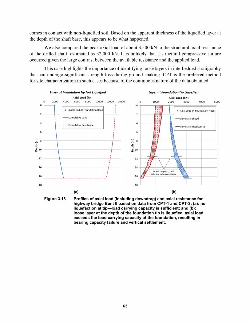
63

comes in contact with non-liquefied soil. Based on the apparent thickness of the liquefied layer at the depth of the shaft base, this appears to be what happened.

We also compared the peak axial load of about 3,500 kN to the structural axial resistance of the drilled shaft, estimated as 32,000 kN. It is unlikely that a structural compressive failure occurred given the large contrast between the available resistance and the applied load.

This case highlights the importance of identifying loose layers in interbedded stratigraphy that can undergo significant strength loss during ground shaking. CPT is the preferred method for site characterization in such cases because of the continuous nature of the data obtained.

(a) (b)

Figure 3.18 Profiles of axial load (including downdrag) and axial resistance for highway bridge Bent 6 based on data from CPT-1 and CPT-2: (a): no liquefaction at tip—load carrying capacity is sufficient; and (b): loose layer at the depth of the foundation tip is liquefied, axial load exceeds the load carrying capacity of the foundation, resulting in bearing capacity failure and vertical settlement.

0

2

4

6

8

10

12

14

16

18

0 1000 2000 3000 4000 5000

Depth (m)

Axial Load (kN)

Layer at Foundation Tip Liquefied

Axial Load @ Foundation Head

Cumulative Load

Cumulative Resistance

0

2

4

6

8

10

12

14

16

18

0 2000 4000 6000 8000 10000 12000 14000

Depth (m)

Axial Load (kN)

Layer at Foundation Tip Not Liquefied

Axial Load @ Foundation Head

Cumulative Load

Cumulative Resistance

Due to range of su,r and adhesion factors considered

65

4 Conclusions

Equivalent static analysis (ESA) procedures for evaluating the effects on bridges of lateral spreading displacements [Ashford et al., 2011; Caltrans, 2013a] have been applied to two adjacent bridges that exhibited different performance levels in similar soil conditions and under approximately the same lateral spreading demands. These procedures correctly predicted the observed behavior of both bridges. The difference in behavior of the two bridges can ultimately be attributed to the cumulative lateral resistance of the railroad bridge pile group being less than the fully-mobilized passive pressure demand from the laterally spreading crust, whereas the highway bridge foundations had sufficient strength and flexural stiffness to resist the passive pressure without undergoing significant displacement. The ESA procedures correctly predicted the response of both bridges using a common framework for assigning input parameters.

The effects of displacement-based inertial demand were found to be negligible in comparison to kinematic loads from lateral spreading, which dominated the response of both bridges. This is expected for bridges that are restrained against translation in the direction of lateral spreading. Force-based methods for combining inertial demands with lateral spreading for models that only included below-ground foundation elements of the bridges did not capture the observed behavior of the bridges and in some cases predicted collapse where none occurred. We recommend using a spectral-displacement-based approach—as opposed to the current force-based approach—to impose inertial demand that explicitly considers the translational and rotational restraint provided by other bridge components.

To adequately assess the predictive capability of the ESA procedures in the context of this case study, it was necessary to model the above-ground components of the bridge bents in addition to the foundation elements. OpenSees provides far more flexibility in structural modeling compared with tools commonly used by geotechnical engineers such as LPILE. It is difficult to accurately predict foundation and superstructure performance when analyses of the two systems are performed independently because the complex interaction that occurs between them cannot easily be replaced by simple shear, moment, or displacement boundary conditions. We therefore recommend performing such simulations using a structural design software package that can capture these more complex features of the structural behavior. This approach will have the added benefit of facilitating better communication between structural and geotechnical designers.

66

The foundation response predicted by the ESA procedures can be sensitive or insensitive to virtually any of the input parameters, and in most cases it is difficult to assess this sensitivity a priori without actually performing parametric studies over a range of the input values. The ESA should be utilized as a tool to understand the performance of a proposed design and guide further geotechnical investigation as well as to facilitate interaction with the bridge superstructure designers.

67

REFERENCES

AASHTO (2009). Guide Specifications for LRFD Seismic Bridge Design, 2nd ed., American Association of State Highway Transportation Officials, Washington D.C.

AASHTO (2012). LRFD Bridge Design Specifications, 6th ed., American Association of State Highway Transportation Officials, Washington D.C.

API (1993). Recommended Practice for Planning, Design, and Constructing Fixed Offshore Platforms, API RP 2A-WSD, 20th ed., American Petroleum Institute, API Publishing Services, Washington D.C.

Ashford S.A., Boulanger R.W., Brandenberg S.J. (2011). Recommended design practice for pile foundations in laterally spreading ground, PEER Report 2011/04, Pacific Earthquake Engineering Research Center, University of California, Berkeley, CA, 43 pgs.

Bolton M.D. (1986). The strength and dilitancy of sands, Géotechnique, 36(1): 6578. Boore D.M., Stewart J.P., Seyhan E., Atkinson G.M. (2014). NGA-West 2 equations for predicting PGA, PGV, and

5%-damped PSA for shallow crustal earthquakes, Earthquake Spectra, DOI: http://dx.doi.org/10.1193/070113EQS184M (in press).

Boulanger R.W., Brandenberg S.J. (2004). Neutral plane solution for liquefaction-induced down-drag on vertical piles. Proceedings, Geotechnical Engineering for Transportation Projects, Geotechnical Special Publication No. 126, M.K. Yegian and E. Kavazanjian, eds., ASCE, pp. 403–410.

Boulanger R.W., Chang D., Brandenberg S.J., Armstrong R.J., Kutter B.L. (2007). Seismic design of pile foundations for liquefaction effects, Proceedings, 4th Int. Conf. on Earthquake Geotechnical Engineering— Invited Lectures, K.D. Pitilakis, ed., Springer, Netherlands, pp. 277–302.

Brandenberg S.J. (2005). Behavior of Pile Foundations in Liquefied and Laterally Spreading Ground, Ph.D. thesis, Department of Civil and Environmental Engineering, University of California, Davis, CA.

Brandenberg S.J., Bellana N., Shantz, T. (2010). Shear wave velocity as function of standard penetration test resistance and vertical effective stress at California bridge sites, Soil Dyn. Earthq. Eng., 30 (10): 1026–1035.

Brandenberg S.J.,Boulanger R.W.,Kutter B.L., Chang D.(2007).Liquefaction-induced softening of load transfer between pile groups and laterally spreading crusts, J. Geotech. Geoenviron. Eng., ASCE, 133(1): 91–103.

Brothers D.S., Driscoll N.W., Kent G.M., Harding A.J., Babcock J.M., Baskin R.L. (2009). Tectonic evolution of the Salton Sea inferred from seismic reflection data. Nat. Geosci., 2(8): 581–584. doi:10.1038/ngeo590.

Brown D., Turner J.P., Castelli R. (2010) Drilled shafts: construction procedures and LRFD design methods, FHWA/NHI Publication 10-016, Reference Manual and Participants Guide for National Highway Inst. Course 132014, 972 pgs.

Caltrans (2013a). Guidelines on Foundation Loading and Deformation due to Liquefaction Induced Lateral Spreading, California Department of Transportation, Sacramento, CA, available: http://www.dot.ca.gov/research/structures/peer_lifeline_program/. Originally published 2011; revised 2013.

Caltrans (2013b). Seismic Design Criteria, California Department of Transportation, Sacramento, CA, available: http://www.dot.ca.gov/hq/esc/techpubs/manual/othermanual/other-engin-manual/seismic-design-criteria/sdc.html.

Cetin K.O., Seed, R.B., Der Kiureghian, A., Tokimatsu, K., Harder, L.F., Kayen, R.E., Moss, R.E. (2004). SPT-based probabilistic and deterministic assessment of seismic soil liquefaction potential. J. Geotech. Geoenviro Eng., 130(12): 1314-1340.

Cetin K.O., Bilge H.T. (2012). Cyclic large strain and induced pore pressure models for saturated clean sands, J. Geotech. Geoenviro. Eng., 138(3): 309-323.

Chu D., Stewart J.P.,Youd T.L., Chu B. (2006). Liquefaction-induced lateral spreading in near-fault regions during the 1999 Chi-Chi, Taiwan earthquake, J. Geotech. Geoenviron. Eng., ASCE, 132(12): 1549–1565.

Colin J.G. (2002). Timber Pile Design and Construction Manual, Timber Piling Council of the American Wood Preservers Institute, Fairfax, VA, 145 pgs.

Davenport C., Fonseca I., Cruz P., de La Pena A. (1981). Cerro Prieto Geothermal Field, CFE’s Geophysical Studies (Internet White Paper). Retrieved from http://terraplus.ca/ch/recon/dave5.aspx.

DeJong J.T., Fritzges M.B., Nusslein K. (2006). Microbially induced cementation to control sand response to undrained shear, J. Geotech. Geoenviron. Eng., ASCE, 132(11): 1381–1392.

68

Dibblee T.W. (1984). Stratigraphy and tectonics of the San Felipe Hills, Borrego Badlands, Superstition Hills, and vicinity, in The Imperial Basin; Tectonics, Sedimentation, and Thermal Aspects, Rigsby, A.C. (ed.), Society of Economic Paleontologists and Mineralogists, Pacific Section, Los Angeles, CA, 40: 45–70.

Dobry R., Taboada V., Liu L. (1995). Centrifuge modeling of liquefaction effects during earthquakes, Proceedings, 1st International Conference on Earthquake Geotechnical Engineering, K. Ishihara, ed., A.A. Balkema, Rotterdam, 3: 1291–1324.

Dorsey R.J. (2010). Sedimentation and crustal recycling along an active oblique-rift margin: Salton Trough and northern Gulf of California, Geology, 38(5): 443–446, doi:10.1130/G30698.1.

EERI (2010). The El Mayor Cucapah, Baja California earthquake, April 4, 2010, Earthquake Engineering Research Institute, J. Meneses, ed., EERI Reconnaissance Report 2010-02, available: http://www.eeri.org.

Faris A.T. (2004). Probabilistic Models for Engineering Assessment of Liquefaction-Induced Lateral Spreading Displacements, Ph.D. thesis, Department of Civil and Environmental Engineering, University of California, Berkeley, CA, 436 pgs.

Faris A.T., Seed R.B., Kayen R.E., Wu J. (2006). A semi-empirical model for the estimation of maximum horizontal displacement due to liquefaction-induced lateral spreading, Proceedings, 8th National Conference on Earthquake Engineering, Earthquake Engineering Research Institute, San Francisco, CA.

Fellenius B.H. (1972). Downdrag on long piles in clay due to negative skin friction, Can. Geotech. J., 9(4): 323–337.

GEER (2010). Preliminary report on seismological and geotechnical engineering aspects of the April 4 2010 Mw 7.2 El Mayor-Cucapah (Mexico) earthquake, Geotechnical Extreme Event Reconnaissance, J.P. Stewart and S.J. Brandenberg, eds., Report No. GEER-023, available: http://www.geerassociation.org/GEER_Post%20EQ%

Hauksson E., Stock J., Hutton K., Yang W., Vidal-Villegas J., Kanamori H. (2011). The 2010 M 7.2 El Mayor-Cucapah earthquake sequence, Baja California, Mexico and Southernmost California, USA: active seismotectonics along the Mexican Pacific Margin, Pure Appl. Geophys., 168(8/9), 1255–1277, doi:10.1007/s00024-010-0209-7.

Hogenstad E., Hanson N.W., McHenry D. (1955). Concrete stress distribution in ultimate strength design, J. Am. Concr. Inst., 25(4): 455–479.

Hough S.E.; Elliot A. (2004). Revisiting the 23 February 1892 Laguna Salada earthquake, Bull. Seismol. Soc. Am.,

94(4): 15711578. Idriss I.M., Boulanger R.W. (2006). Semi-empirical procedures for evaluating liquefaction potential during

earthquakes, J. Soil Dyn. Earthq. Eng., 26(2–4): 115–130. Idriss I.M., Boulanger R.W. (2008). Soil Liquefaction during Earthquakes, Monograph MNO-12, Earthquake

Engineering Research Institute, Oakland, CA. Ishihara K., Yoshimine M. (1992). Evaluation of settlements in sand deposits following liquefaction during

earthquakes, Soils Found., 32(1): 173–188. Jaky J. (1948). Pressure in silos, Proceedings, 2nd International Conference on Soil Mechanics and Foundation

Engineering, Balkema, Rotterdam, 1: 103–107. Kramer S. (2013). Personal communication. Kwak D.Y., Mikami A., Brandenberg S.J., Stewart J.P. (2012). Ground motion estimation for evaluation of levee

performance in past earthquakes, Proceedings, 9th International Conference on Urban Earthquake Engineering./4th Asis Conference on Earthquake Engineering, Center for Urban Earthquake Engineering, Tokyo Institute of Technology, Tokyo, Japan.

Kulhawy F.H., Mayne P.W. (1990). Manual on Estimating Soil Properties, Report EL-6800, Electric Power Research Institute, Palo Alto, CA.

Lysmer J. (1970). Lumped mass method for Rayleigh waves, Bull. Seismol. Soc. Am., 60(1): 89–104. Marcuson W.F., Hynes M.E., Franklin A.G. (1990). Evaluation and use of residual strength in seismic safety

analysis of embankments, Earthq. Spectra, 6(3): 529–572. Martin G.R., Marsh L.M., Anderson D.G., Mayes R.L., Power M.S. (2002). Recommended design approach for

liquefaction induced lateral spreads, Proceedings, 3rd National Seismic Conference and Workshop on Bridges and Highways, Portland, OR.

McCrink T.P., Pridmore C.L., Tinsley J.C., Sickler R.R., Brandenberg, S.J., Stewart J.P. (2011). Liquefaction and other ground failures in Imperial County, California, from the April 4, 2010, El Mayor–Cucapah earthquake, U.S. Geological Survey Open-File Report 2011–1071 and California Geological Survey Special Report 220, 94 pgs. pamphlet,1 pl., scale 1:51,440, available: http://pubs.usgs.gov/of/2011/1071/ .

69

McKenna F.T. (1997). Object-Oriented Finite Element Programming: Frameworks for Analysis, Algorithms and Parallel Computing, Ph.D. thesis, Department of Civil and Environment Engineering, University of California, Berkeley, CA.

Merriam R., Bandy O.L. (1965). Source of upper Cenozoic sediments in Colorado Delta region, J. Sediment. Res., 35(4): 911–916. doi:10.1306/74D713A2-2B21-11D7-8648000102C1865D.

Mosher R.L. (1984). Load Transfer Criteria for Numerical Analysis of Axial Loaded Piles in Sand, U.S. Army Engineering and Waterways Experimental Station, Automatic Data Processing Center, Vicksburg, Miss.

Ovesen N.K. (1964). Anchor slabs, calculation methods and model tests, Bulletin No. 16, The Danish Geotechnical Institute, Copenhagen, Denmark.

Pacheco M., Martín-Barajas A., Elders W., Espinosa-Cardeña J.M., Helenes J., Segura, A. (2006). Estratigrafía y estructura de la cuenca de Altar del NW de Sonora: implicaciones para la historia del delta del Río Colorado y de la cuenca Salton, Revista mexicana de ciencias geológicas, 23(1): 1–22.

PEER (2013). NGA-West2 database flatfile, Pacific Earthquake Engineering Research Center, available: http://peer.berkeley.edu/ngawest2/databases/. Last accessed 20 November 2013.

Reese L.C., Wang S.T., Isenhower W.M., Arrelaga J.A., Hendrix J.A. (2005). LPILE plus version 5.0. Ensoft, Inc., Austin, TX.

Robertson P.K., Wride C.E. (1998). Evaluating cyclic liquefaction potential using the cone penetration test, Can, Geotech. J., 35(3): 442–459.

Robinson P.K., Bradley B.A., Cubrinovski M. (2012). Analysis of liquefaction-induced lateral spreading data from the 2010 Darfield and 2011 Christchurch earthquakes, Proceedings, NZSEE Annual Technical Conference & AGM, Christchurch, New Zealand.

Robertson P.K. (2010). Evaluation of flow liquefaction and liquefied strength using the cone penetration test, J. Geotech. Geoenviron. Eng., ASCE, 136(6): 842–853.

Robertson P.K. (2012). Interpretation of in-situ tests—some insights, Proceedings, 4th International Conference on Geotechnical and Geophysical Site Characterization (ISC-4), R.Q. Coutinho and P.W. Mayne, eds., Pernambuco, Brazil, 22 pgs.

Rodriguez-Marek A., Montalva G.A., Cotton F., Bonilla F. (2011). Analysis of single-station standard deviation using the KiK-net data, Bull. Seismol. Soc. Am., 101: 1242–1258.

Salgado R. (2006). The Engineering of Foundations, McGraw-Hill, New York. 882 pgs. SCT (2013). Personal communication, Secretaría de Comunicaciones y Transportes. TRC Software (2011). XTRACT cross section analysis program for structural engineers, Rancho Cordova,

California. http://www.imbsen.com/software-XTRACT.html. USGS (2010). Magnitude 7.2 Baja California, Mexico, earthquake information, U.S. Geological Survey, available:

http://earthquake.usgs.gov/earthquakes/eqinthenews/2010/ci14607652/ Last accessed 20 November 2013. USGS (2014). ShakeMap Background, U.S. Geological Survey available:

http://earthquake.usgs.gov/research/shakemap/ Last accessed March 10, 2014. Vijayvergiya V.N. (1977). Load-movement characteristics of piles, Proceedings, Ports '77: 4th Annual Symposium

of the Waterway, Port, Coastal, and Ocean Division, Long Beach, CA, pp. 269284. Wang R., Brandenberg S.J. (2013). "Beam on nonlinear Winkler foundation and modified neutral plane solution for

calculating downdrag settlement." J. Geotech. Geoenviron. Eng., 139(9), 1433-1442. Wei S., Fielding E., Leprince S., Sladen A., Avouac J.P., Helmberger D., Briggs R. (2011). Superficial simplicity of

the 2010 El Mayor-Cucapah earthquake of Baja California in Mexico, Nat. Geosci., 4(9): 615–618. doi:10.1038/ngeo1213.

Yang Z. and Jeremić B. (2002). Numerical analysis of pile behavior under lateral loads in layered elasticplastic soils, Int. J. Numer. Anal. Geomech., 2: 131.

Youd T.L., Hansen C.M., Bartlett S.F. (2002). Revised multi-linear regression equations for prediction of lateral spread displacement, J. Geotech. Geoenviron. Eng., ASCE, 128(12): 1007–1017.

Zhang G., Robertson P.K., Brachman R.W.I. (2002). Estimating liquefaction induced ground settlements from CPT for level ground. Can. Geotech. J., 39: 1168–1180.

Zhang G., Robertson, P.K., Brachman R.W.I. (2004). Estimating liquefaction-induced lateral displacements using the standard penetration test or cone penetration test, J. Geotech. Geoenviron. Eng.,ASCE, 130(8): 861–871.

71

Appendix A: Subsurface Investigations

73

Dep

th [m

]

74

Dep

th [m

]

75

Dep

th [m

]

76

Log of boring performed for Ferromex near Bent 5 of railroad bridge. Exact location unknown. Provided by SCT (personal communication, 2013).

77

Appendix B: Laboratory Test Results

81

Appendix A: Sample Calculations

This appendix presents a portion of the calculations that were performed in order to quantify the input parameters used for the finite-element analysis described in the main report. Not all calculation are shown. The reader is encouraged to refer to the references cited in the report rather than simply changing the numbers in these sample calculations to fit their project. Section numbers refer to the section number in the main report in which the calculations being shown here are discussed. Note: trigonometric functions shown herein accept angles in radians as the argument.

Section 3.1 Soil Properties

Soil properties presented in Table 3.1 of the report are primarily based on correlations to CPT measurements. Correlations were performed at each depth corresponding to the sampling interval of the CPT (every 1 cm), and then the correlated values were averaged over the depth interval of each layer of interest. Examples are provided below of the correlations for a single discrete depth interval. Using data from CPT-1, at a depth of 3 m below ground surface: d = 3 (depth – 3 m).

Stress

1.5 17 1.5 18 52.5v

Vertical total stress in kPa—see Table 3.1 for unit wt.

1.5 17 1.5 18 9.81 37.8vp Vertical effective stress in kPa

101.325ap Atmopheric pressure in kPa

Penetration resistance: multiple methods will be used so that correlations to soil properties (e.g., relative density) can use the appropriate corrected penetration resistance as input.

3468tq Measured cone tip resistance in kPa

Robertson [2012]:

1.928cI

Soil behavior type index, stress exponent, and overburden normalized cone tip resistance, respectively, using Robertson’s [2012] approach—note: requires iteration to determine stress exponent and soil behavior type index.

0.6n

61.1tnQ

3 4 25.581 0.403 21.63 33.75 17.88 1.22c c c c cK I I I I Clean sand factor for cI >1.64 [Robertson

2012; Eqn. 22]

, 74.3tn cs c tnQ K Q Equivalent clean sand overburden normalized

82

cone tip resistance [Robertson 2012; Eqn. 20]

60 1.1268 0.28179

10 c

t aI

q pN

Equivalent STP N-value at 60% energy [Robertson 2012; Eqn. 2]

1 58IB IBc N N t aq C q p

1.6 because 2.68 is 1.6N a vpC p SPT overburden correction factor [Cetin 2004]

1 6060 14NN C N Overburden and energy corrected equivalent SPT blowcout

Robertson and Wride [1998] method with Zhang [2002] update:

1.81 2n

q a vpC p Overburden correction factor

1 62RWZ

c N q t aq C q p

Overburden corrected normalized cone penetration resistance (RWZ subscript indicates Robertson and Wride [1998] method with Zhang [2002] updates

Idriss and Boulanger [2006; 2008] method—requires iteration

Initial guess for exm stress exponent : 0.5exm

1.64 1.7 therefore 1.6ex exm ma vp NIB a vpp C p

IBNC is the Idriss and Boulanger overburden

correction factor

Evaluate 1 IBc Nq using this correction factor:

1 56 254IB IB

tc N N

a

qq C

p

Now re-compute the stress exponents, m , using this normalized cone pentration resistance:

0.26411.338 0.249 0.62

IBex c Nm q

Re-compute the overburden correction factor:

1.84 1.7 therefore 1.7ex

IB

ma vp Np C

Re-compute normalized penetration resistance:

1 58 254IB IB

tc N N

a

qq C

p

Re-compute m and IBNC

0.26411.338 0.249 0.61 1.83 1.7 1.7ex

IBIB

mex a vp Nc Nm q p C

Re-compute normalized penetration resistance

83

1 58 254IB IB

tc N N

a

qq C

p

After three iterations, the values of m and

IBNC , and the overburnden corrected normalized cone penetration

resitance have stabilized.

2.62.8 15cFC I Estimated fines content. Is reasonable based on SCT boring logs.

21

19.7 15.7

5.4 exp 1.63 3116 .01 .01

IB

IB

c Nc N

qq

FC FC

Clean sand correction factor

1 , 1 1 89IB IB IBc N cs c N c Nq q q

Equivalent clean sand overburden corrected normalized resistance (IB subscript indicated in Idriss and Boulanger method [2006; 2008]

Correlated parameters

Friction angle

32cv Constant volume (critical state) friction angle depending on minerology, taken as 32 for quartz sand.

,15.84 log 26.88 35cv tn csQ Peak friction angle [Robertson 2012, Eqn. 25]

Relative density—use multiple correlations, then take a weighted average

Idriss and Boulanger [2008] methods:

0.2641 60

10.56 0.478 1.063 0.3346IBspt IBcpt IBR R c N

ND D q

Relative density based on correlations to SPT and CPT penetration resistances, respectively.

Zhang et al. [2008] method:

11

85 76 log0.51for 200

100RWZ

Zhang

c NR c N

qD q

Kulhawy and Mayne [1990] method

10.44

325RWZ

KM

c NR

qD

Weighted average of the computed relative densities:

0.3 0.3 0.1 0.3 0.48IBspt Zhang IBcpt KMR R R R RD D D D D

The Idriss and Boulanger [2008] method using CPT as the input consistantly predicted lower RD values

compared to the other three methods, so it was assigned a lower weighting factor. Judgment should always be applied when consisdering which correlations provide the most reliable estimates for a given project

84

Liquefaction susceptibility and triggering analysis

Note: use the appropriate normalized penetration resistance for each calculation. For example, do not use the

Robertson [2012] ,tn csQ values for the Idriss and Boulanger [2008] liquefaction triggering analysis; use the Idriss

and Boulanger [2008] 1c Nq

Idriss and Boulanger [2008] methods:

Susceptibility:

1.93 2.6cI

…therefore, susceptible. In addition, our index testing determined that the fines portion of the bulk sample we collected near the surface is nonplastic. The sample is considered to be reasonably similar to the soil at 3 m depth being considered herein. The conclusion is that the soil at this depth is susceptible to liquefaction. Conclusion: soil at this depth is suceptible to liquefaction.

Triggering:

7.2M Earthquake magnitude being considered (in this case magnitude of 2010 EMC earthquake)

PGA = 0.27 Peak ground acceleration estimated for SFB site

1 , 89IBc N csq Normalized cone penetration resistance to be used

for compuations

Nonlinear stress reduction factor, dr :

1.012 1.126sin 5.133 0.13411.73z

d

0.106 1.118sin 5.142 0.01511.28z

d

exp 0.977 0.98d z z dr M r Check-- should be close to 1.0 near the ground surface

0.65 ( ) 0.238v vp dCSR PGA r Cyclic stress ratio (CSR) is estimate of demand

Overburden correcton factor:

0.2641 ,

10.097 0.3

37.3 8.27

1 ln 1.096 1.1 therefore 1.1

IBc N cs

vp

a

Cq

K C Kp

[Idriss and Boulanger 2006]

Assume ground is approx. level such that the static shear stress correction factor is 1.0: 1.0K .

Compute cyclic resistance ratio (CRR) for M 7.5, 1 atm. of effective overburden pressure and level ground:

1

2 3 41 , 1 , 1 , 1 ,

7.5 exp 3 0.125540 67 80 114

IB IB IB IBc N cs c N cs c N cs c N csM

q q q qCRR

Compute magnitude scaling factor:

85

6.9 exp 0.58 1.0834

MMSF

Correct CRR for appropriate value of earthquake magnitude and effective overburden stress:

17.5 0.148MCRR CRR MSF K

Compute factor of safety against liquefaction

0.62 1liqCRR

FSCSR

Solution: soil is predicted to liquefy during the M7.2 EMC earthquake with a PGA of 0.27g

Post-liquefaction behavior

Estimate shear strain resulting from liquefaction [Idriss and Boulanger 2008]

30.264lim 1 ,1.859 2.163 0.478 0.4 0.5

IBc N csq Limiting shear strain (%)

0.264 0.5281 , 1 ,11.74 8.34 1.37 0.87

IB IBc N cs c N csF q q Parameter F

1liqFS F Since the factor of safety against liquefaction is less than parameter F , the estimated shear strain is taken

as the limiting shear strain.

max lim 0.4

Post-liquefaction residual undrained shear strength:

,

2, ,

0.02199 0.00031211.7

1 0.02676 0.0001783

tn csur vp

tn cs tn cs

Qs

Q Q

Robertson [2010]

0.03 tan 1180ur vps

Check that estimated value is greater than 0.03 and less than the shear strength under static conditions using the estiamted friction angle. Evaluation of inequality is “true” (=1)

Excess porewater pressure ratio: Since soil at depth = 3 m is predicted to liquefy, assume ur = 100%. For layers

with estimated 1.0liqFS , ur was estimated using a hyperbolic decay function fit to the Marcuson et al. [1990] plot

of liqFS versus ur , and for comparison, the Cetin and Bilge [2012] relationship between shear strain and ur . The

methods were found to provide similar results for liqFS substantially greater than 1.0. The Marcuson et al. equation

is presented below as an example for 1.7.liqFS

1.7liqFS 1

0.091 14 1

EX

uliq

rFS

P-multiplier for fully liquefied condition ( ur = 100%), using the equation from Figure 3.7 in the Caltrans lateral

spreading guideslines [2013a].

First compute equivalent clean sand (N1)60 value using the Idriss and Boulanger [2008] equations:

86

1 60

2

1 60

1 1 160, 60 60

2

1 160, 60,

14

9.7 15.7exp 1.63 3

0.01 0.01

18

0.0031 0.00034 0.16

cs

p cs cs

N

NFC FC

N N N

m N N

For layers with predicted factor of safety against liquefaction greater than 1.0, there is still excess porewater pressure build-up, which reduces effective stress and acts to soften load transfer. To account for this, a p-multiplier is determined based on a linear interpolation between the estimated ur of 100% and the

corresponding fully-liquefied p-multiplier (previous calculation). For example:

1

1.7 0.091 14 1

EX

liq uliq

FS rFS

1 60,

2

1 160, 60,

33

0.0031 0.00034 0.47

cs

p cs cs

N

m N N

(Fully liquefied p-multiplier)

1 1 0.95pNonLiq u pm r m Interpolated p-multiplier to account for decreased effective stress

Computations for a non-liquified crust p-y springs following Caltrans lateral spreading guidelines [2013a]. For a graphical explation of the dimensions, refer to Figure 3.2 in the Caltrans guidelines.

Highway Bridge

4cN Number of extended-shaft columns

1.2B Shaft diameter (meters)

0D

Crust thickness above top of transverse diaphragm (meters). Assume no flow between the short length of the shafts between the top of the transverse diaphragm and the ground surface such that the transverse diaphragm essentially extends to the surface

1.5T Transverse diaphragm height (meters)

1.5cZ Non-liquefied crust thickness (meters)

0bbZ Distance between bottom of transverse diaphragm and bottom of crust (meters)

1.5t cZ Z D

Distance between the top of the transverse diaphragm and bottom of crust (meters)

10.2tW Width of the transverse diaphragm in the bridge transverse direction (meters)

1.2LW Width of the transverse diaphragm in the bridge longitudinal direction (meters)

2.55ttrib

c

WW

N Tributary width of the tranverse diaphragm assigned to the single shaft being

analyzed (meters)

87

Soil properties in non-liquified crust:

35 Peak friction angle

0.5 17 13vp cZ Effective stress at mid-height of the crust layer (kPa); soil unit wt. in 17 kN/m3

Lateral earth pressure coefficients

2

tan 45 3.69180 2pK

Rankine passive L.E.P. coefficient

2

tan 45 0.27180 2pK

Rankine active L.E.P. coefficient

3

42/3

0.4 11.6

1 1.1 1 1.10.05

1 5 1

p a

w p at t

TK K

T D Tk K K

W WD T

T T

Adjustment factor for 3D wedge-shaped failure surface

Compute forces from crust acting against bent:

795passiveCap vp p t wF K T W k Passive force acting against “front” face of composite block formed by extended-shaft columns and transverse diaphragm (kN)

2 tan 9180 3sidesCap vp L tF W Z

Force acting on sides of outside extended-shaft columns through the crust (kN)

The non-liquefied crust does not extend below the base of the transverse diaphragm, therefore, the foundations do not contribute to the resistance within the crust: 0pilesF

804ultGroup passiveCap sidesCapF F F The total force is the sum of the passive and side forces (kN)

201ultGroup

ultInvidualc

FF

N

This is the total force acting on a single extended-shaft column’s tributary width within the crust.

Determine displacement required to fully mobilize the non-liquefied crust passive pressure. Considers a softened load-transfer relationship for crust overlying liquified layer [Brandenberg 2007].

Factors relating thickness of crust relative to width and thickness of pile cap

4

1exp 3 1 1 0.58

101

4

cdepth width

t

Z Df f

T

W

T

max 0.05 0.45 0.46depth widthT f f Estimated displacement (meters) required to mobilized full passive pressure

As shown in the Caltrans lateral spreading guidelines [2013a] (Figure 3.1), the load transfer curve for the crust is represented with a trilinear curve defined by three points: (1) the origin; (2) half of the ultimate force and ¼ of the displacement required for full passive mobilization; and (3) the ultimate force and the full displacement. The curve then continue at zero slope for further displacement. Note that the displacement in this case refers to the relative displacement between the soil and the structure, not the absolute displacement of the laterally spreading ground.

88

max

max

max

00

0.124

0.46

2.325

refDisp

00

1012

201

201

ultIndividual

ultIndividual

ultIndividual

FForce

F

F

When lateral load-transfer is represented through p-y curves, it is customary to express the load as force per unit length of the foundation.

HWB HWB relc

Forcep y Disp

Z D

See p-y curve below

Railroad Bridge (same procedure)

0D

Crust thickness above top of pile cap (meters). Since oblong pier-wall-type column is nearly as wide as the pile cap, assume a uniform block of soil will exert passive pressure from the base of the pile cap to the ground surface

1.5T Effective pile cap height (meters)

1.5cZ Non-liquefied crust thickness (meters)

0bbZ Distance between bottom of pile cap and bottom of crust (meters)

1.5t cZ Z D Distance between the top of the pile cap and bottom of crust (meters)

6.5tW Width of the pile cap in the bridge transverse direction (meters)

4.6LW Width of the pile cap in the bridge longitudinal direction (meters)

Soil properties in non-liquified crust same as for HWB:

Lateral earth pressure coefficients

3.69 0.27p aK K

Rankine passive and active L.E.P. coefficient

3

42/3

0.4 11.6

1 1.1 1 1.160.05

1 5 1

p a

w p at t

TK K

T D Tk K K

W WD T

T T

Adjustment factor for 3D wedge-shaped failure surface

Compute forces from crust acting against bent:

532passiveCap vp p t wF K T W k Passive force acting against “front” face of composite block formed by pile cap and oblong column (kN)

2 tan 36180 3sidesCap vp L tF W Z

Force acting on sides of pile cap (kN)

The non-liquefied crust does not extend below the base of the pile cap, therefore, the foundations do not contribute to the resistance within the crust: 0pilesF

569ultGroup passiveCap sidesCapF F F The total force is the sum of the passive and side forces (kN)

Determine displacement required to fully mobilize the non-liquefied crust passive pressure.

Factors relating thickness of crust relative to width and thickness of pile cap

89

4

1exp 3 1 1 0.33

101

4

cdepth width

t

Z Df f

T

W

T

max 0.05 0.45 0.29depth widthT f f Estimated displacement (meters) required to mobilized full passive pressure

max

max

max

0 00 0

0.07 2844 2

0.29 569

1.47 5695

ultIndividual

ref

ultIndividual

ultIndividual

FDisp Force

F

F

Express the load as force per unit length (in vertical direction) of the structure:

RRB RRB relc

Forcep y Disp

Z D

Section 3.2 Magnitude of Lateral Spreading Displacement

Lateral spreading index using the Zhang [2004] method as presented in Idriss and Boulanger [2008]:

0.01layert Thickness of each layer for calculation is 1 cm (i.e., the CPT sampling interval

max 0.00401i layerLDI t This is the predicted lateral spreading (LDI) for the 1-cm-thick layer at a depth of 3 m. This computation is repeated at each CPT sampling interval from the “bottom up” to generate a profile of cumulative LDI versus depth. LDI is then converted to an estimated lateral spreading displacement via a multiplicative factor that depends on the ground slope and the free-face conditions. Refer to the main report and Zhang [2004] for more details.

0 0.2 0.4 0.6 0.80

100

200

300

400

Highway BridgeRailroad Bridge

Nonliquefied Crust p-y Curves

Relative Displacement (m)

Loa

d (k

N/m

)

90

Lateral spreading index using the modified Faris [2006] method as presented in the Caltrans lateral srpeading guidelines [2013a].

Lateral spreading is assumed to occur up to a depth of two times the free-face height, about 7 m, meaning only the upper liquefied layer should be considered. For the upper liquefied layer (depth 1.5 to 6.5 m below

ground surface), the average 1 60N value (using the methods presented above) is 12. Using an estimated

fines content erange of 1520%, the fines correction factor is:

2

1 609.7 15.7

15 exp 1.63 3.30.1 0.1lower low

lower lowerFC N

FC FC

2

1 609.7 15.7

20 exp 1.63 4.50.1 0.1upper up

upper upperFC N

FC FC

An approximate average of 4 will be used:

1 1 160 60, 604 12 16avg cs avgN N N

An additional correction factor based on fines content is recommendation by Faris et al. [2004] to generate a corrected blowcount for use in estimated shear strain potential:

1 60,0.882 5 19csN Since this is greater than the average estimated fines content, the correction is zero

1 160, 60,0 16FC FCcs csN N N N

Magnitude-corrected CSR

0.238 0.22mcCSR

CSR CSRMSF

Using these values of 1 60,csN and magnitude-corrected CSR with Figure 3.12 from the Caltrans lateral spreading

guidelines [2013a], the estimated strain potential index is about 1011%. Using the equations in Appendix A of the Caltrans guidelines to get a more refined estimate:

1 60, 1/3

11 7.4

0.04

0.56

n csmc

NCSR

1 1 60,

2 1 60,

0.04 0.00207 0.073

0.04 0.00477 0.115

cs

cs

l N

l N

2 1mcCSR l which is true, therefore use:

3

1 60,max 1.859 1.1 0.108

46

ncsCT

N

Compute displacement potential index (DPI):

6.5 1.5max 0.54CTDPI

Estimate maximum displacement from DPI:

91

1.07max 0.52H DPI

Bent 5 is located near the river bank free face (L/H < 4); therefore,the displacement is amplified by a factor of 2:

max max2.0 1.04amp ampF H F H

The estimated displacement at the ground surface is about 1 m using the Caltrans [2013a] approach based on Faris et al. [2004; 2006], significantly less than that Idriss and Boulanger [2008] approach based on Zhang et al. [2004] of about 3.7 m. The difference is due primarily to the difference in shear strain predicted by the two methods. The equivalent clean sand corrected blowcounts used for the Caltrans approach predict an average shear strain of 37% in the layer. The equivalent SPT blowcounts used herein are based on the correlation to CPT resistance shown previously, but it should be noted that the values compare relatively well to the Ferromex boring log for this layer. Ultimately, the large difference between the two predictions illustrates the uncertainty in relating penetration resistance to shear strain potential and the further uncertainty in the empirical factors used to transform the computed displacement index values (DPI or LDI) to actual horizontal displacements.

Section 3.3 Elastomeric Bearings

Determine the rotational and shear stiffness of elastomeric bearings for highway bridge.

ASSHTO approach per ASSHTO LRFD Bridge Specifications, 6th Ed., Chapter 14

0.2 m 0.3 m 0.041 mb b bearingL W t Length, width, and thickness of bearing

32 410.06 m 0.3 m 0.2 m 0.0002 m

12b b b bearingA L W I Area and MOI

900,000 2,000,000,000a bulk aG P K P Shear and bulk moduli

0.041 mri bearingh t

1.463

2b b

iri b b

L WS

h L W

Eqn. 14.7.5.1-1

30.054i

ulk

GS

K

2

2.31 1.86 0.9 0.96 1 min , 2.116b ba

b b

W LB

L W

Eqn. C14.7.5.3.3-7

2

2 2

3 12233696 12233696

59677 (per radian)

kg kN kg1317073 1317 1317000

m

cAASHTO a i a elastomer cAASHTO a

elastomer bearingr

bearing

bshear

bearing

E B G S P E E P

E IK J

t

A GK

t s s

Each bearing has a translational (shear) stiffness of 1317 kN/m. There are 7 bearings at each of the two abutments. The total translational stiffness provided by the abutment bearings is

92

1317 2.7 18438 18.4 MN/m `

Each bent of the highway bridge has four extended-shaft columns, so the “tributary restraint” of a single column is:

18.44 4 4.61 4.6 MN/m

Section 3.3.2: Rotational restraint derived from rotation of top of column, railroad bridge. Refer to Figure 20 in the report for schematic derivation of equations.

1325w Weight of one deck span

0.2 Coefficient of friction for sliding between top of elastomeric bearings and girders

width 1.7BC Width of bent cap in bridge longitudinal direction (meters)

1 Derive rotational stiffness for a unit rotation (one radian)

1

widthcos 304

4BC

cw

M

Rotational stiffness for mechanisms one [kN*m/rad]

2

widthsin 95

4BC

cw

M

Rotational stiffness for mechanism two

1 2 399Totalc c cM M M

Section 3.4 Inertial Loads

Two approaches were taken to estimate the inertial loads that would be applied in combination with kinematic loads from lateral spreading: (1) a displacement-based approach as recommended in the PEER lateral spreading guidelines [Ashford et al. 2010]; and (2) a force-based approach as presented in the Caltrans lateral spreading guidelines [2013a]

1. Displacement-based approach:

a. Estimate first-mode period of bent and tributary portion of superstructure, T1.

b. Determine pseudo-spectral acceleration at period T1 from a design response spectgrum, or in this case from spectra of recorded motions during the 2010 EMC earthquake.

c. Convert pseudo-spectral acceleration to spectral displacement ( )s d

d. Multiply ( )s d by factors liqC and ccC to account for effects of liquefaction and pahsing.

e. Apply the resulting scaled ( )s d to the structure in combination with kinematic loads and perform analysis.

2. Force-based approach:

For both the RRB and the HWB, the columns did not yield at their base. Therefore, the inertial demands cannot be estimated during the column plastic moment capacity; rather, the inertial demand of the superstructure must be estimated directly. Caltrans [2013a] recommends applying 50% of the estimated inertial demands in combination with 100% of kinematic demands.

Railroad Bridge

Superstructure

1 1.10secRRB

T From modal analysis

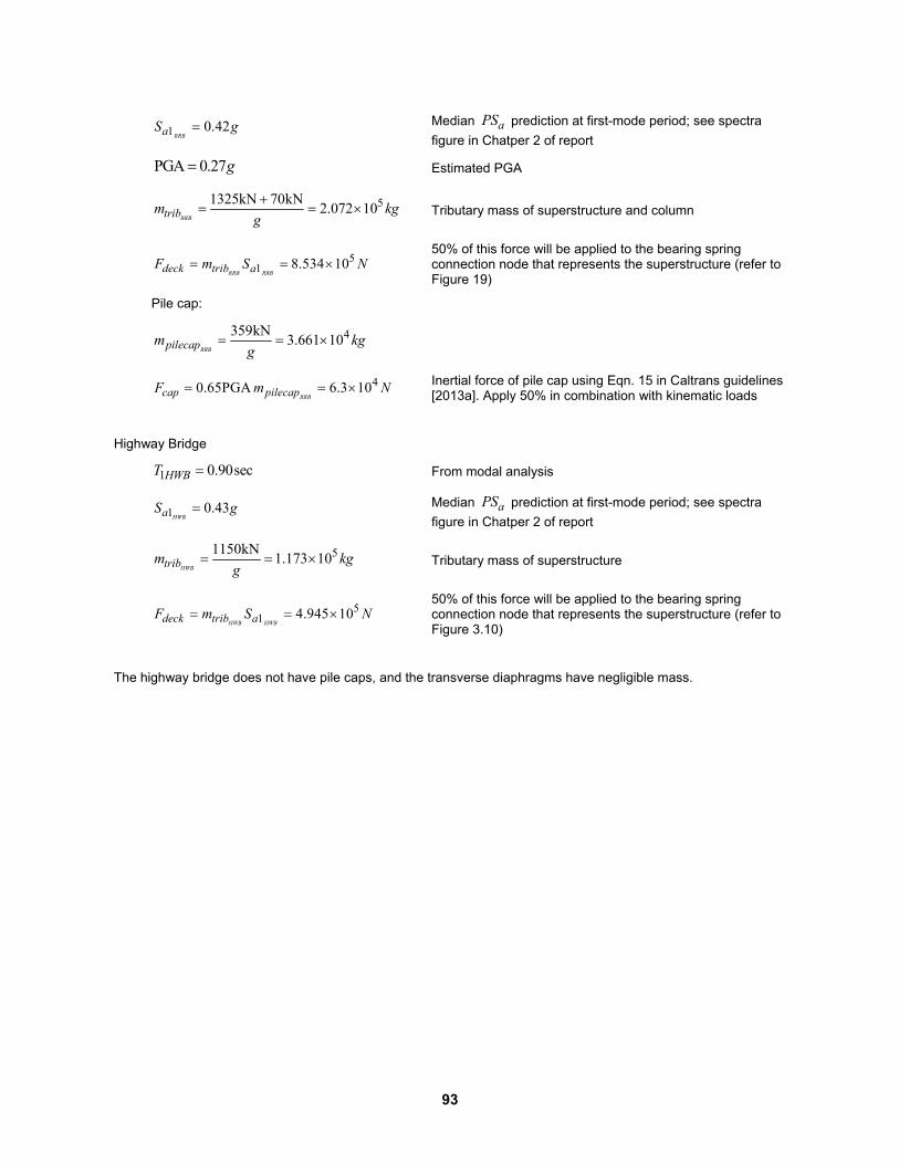
93

1 0.42RRBaS g Median aPS prediction at first-mode period; see spectra

figure in Chatper 2 of report

PGA 0.27g Estimated PGA

51325kN 70kN2.072 10

RRBtribm kgg

Tributary mass of superstructure and column

51 8.534 10

RRB RRBdeck trib aF m S N 50% of this force will be applied to the bearing spring connection node that represents the superstructure (refer to Figure 19)

Pile cap:

4359kN3.661 10

RRBpilecapm kgg

40.65PGA 6.3 10RRBcap pilecapF m N Inertial force of pile cap using Eqn. 15 in Caltrans guidelines

[2013a]. Apply 50% in combination with kinematic loads

Highway Bridge

1 0.90secHWBT From modal analysis

1 0.43HWBaS g Median aPS prediction at first-mode period; see spectra

figure in Chatper 2 of report

51150kN1.173 10

HWBtribm kgg

Tributary mass of superstructure

51 4.945 10

HWB HWBdeck trib aF m S N 50% of this force will be applied to the bearing spring connection node that represents the superstructure (refer to Figure 3.10)

The highway bridge does not have pile caps, and the transverse diaphragms have negligible mass.

The Pacific Earthquake Engineering Research Center (PEER) is a multi-institutional research and education center with headquarters at the University of California, Berkeley. Investigators from over 20 universities, several consulting companies, and researchers at various state and federal government agencies contribute to research programs focused on performance-based earthquake engineering.

These research programs aim to identify and reduce the risks from major earthquakes to life safety and to the economy by including research in a wide variety of disciplines including structural and geotechnical engineering, geology/seismology, lifelines, transportation, architecture, economics, risk management, and public policy.

PEER is supported by federal, state, local, and regional agencies, together with industry partners.

PEER Core Institutions:University of California, Berkeley (Lead Institution)

California Institute of TechnologyOregon State University

Stanford UniversityUniversity of California, DavisUniversity of California, Irvine

University of California, Los AngelesUniversity of California, San DiegoUniversity of Southern California

University of Washington

PEER reports can be ordered at http://peer.berkeley.edu/publications/peer_reports.html or by contacting

Pacific Earthquake Engineering Research CenterUniversity of California, Berkeley325 Davis Hall, mail code 1792

Berkeley, CA 94720-1792Tel: 510-642-3437Fax: 510-642-1655

Email: [email protected]

ISSN 1547-0587X

pacific earthquake engineering research...

Documents