P1-3-8

Avoiding False Amplitude Anomalies by 3D Seismic Trace Detuning

Ashley Francis, Samuel Eckford

Earthworks Reservoir, Salisbury, Wiltshire, UK

Introduction

Amplitude maps derived from 3D seismic interpretation are an important tool for understanding geological changes in the subsurface, including facies or porosity distribution. Many new exploration and near-field drilling targets are associated with an amplitude anomaly, often interpreted as a direct hydrocarbon indicator or DHI.

Many factors affect 3D seismic amplitude and the interpretation of amplitude changes is not unique. However, in the interpretation of seismic amplitude it seems to be widely unappreciated that the biggest factor controlling seismic amplitude variation is not sought-after geological changes or DHIs, but is in fact thickness variation.

This is because seismic amplitudes are affected by tuning, whereby the amplitude responds to reservoir thickness changes independently of any lateral change in the reservoir properties. These amplitude changes are a consequence of constructive and destructive interference of the reflections. While the severity of tuning effects can vary, the bandlimited nature of seismic means that tuning is ever present, even in broadband data. Thickness related tuning can easily double amplitudes, often being the cause of significant reflector brightening in seismic data. By comparison, even a very strong gas saturation effect in a soft sand reservoir may only change amplitudes by 25%.

Thickness related tuning is well understood in geophysics, but the basic principle of removing tuning effects from amplitude maps is not widely applied. Published methods of detuning apply only to maps extracted via seismic picking. In contrast to this approach, this paper shows examples from a new and novel technique which directly detunes the seismic traces in situ. The advantages of direct detuning of 3D seismic volumes (or alternatively 2D seismic lines) include the ability to investigate the whole trace amplitude response (not just a window or extraction), generation of tuning curves without seismic data picking, rapid updating and modification of parameters and improved stratigraphic and quantitative interpretation.

Wedge Model of Tuning

Geophysicists show the effect of tuning using a constant property wedge model. An example of this type of model of a thinning reservoir is shown in Figure 1. This is an example for a soft sand reservoir in the Kadanwari Field, Pakistan. Note that all the layers in this model have constant properties: only the thicknesses are changing, thinning from left to right.

Figure 1(a) Wedge model of a brine saturated sand for the Kadanwari Field, Pakistan

Figure 1(b) Relative acoustic impedance response of brine saturated sand model in 1(a). The modelled reservoir sand appears as the green/yellow event, with the brightening (green) very clear in the centre of the plot

Note that the modelled interval (Figure 1(a)) has constant impedance properties within each layer, but the relative impedance from the seismic model response (Figure 1(b)) is clearly brighter (more green) in the centre and reduces in amplitude (becomes more yellow) as the interval gets thicker or thinner.

Figure 2 is a plot of the amplitude of the reservoir response from Figure 1(b) plotted as a function of TWT thickness. Note how the amplitude reaches a maximum around 13 ms and then falls off to about half the peak amplitude at around 35 ms. This doubling of the amplitude as a function of thickness is the tuning effect.

Figure 2 Tuning curve for Kadanwri brine saturated sand showing amplitude variation as a function of TWT thickness of reservoir

Not shown here, but modelling of the effect of gas in the Kadanwari Field in Pakistan shows that a gas filled reservoir sand would exhibit about a 25% brighter amplitude than a brine filled sand. By comparison, from Figure 2, the effect of changing reservoir thickness from 36 ms down to 13 ms (corresponding to a thickness change from 60 to about 20 m), would be to double the maximum amplitude of the seismic reflection. This demonstrates clearly that thickness related tuning effects are potentially much larger than lateral amplitude variations due to geological changes, including lithology or hydrocarbon fluid effects.

Tuning effects are very predominant in seismic amplitude responses and tend to be the most significant factor affecting amplitude maps. Meaningful interpretation of amplitudes in terms of lateral property changes therefore requires us to first remove the effects of tuning.

Detuning Seismic Traces

The concept of detuning amplitude maps picked from seismic is not new but interest in the topic was recently renewed by Connolly (2007) with a series of presentations and articles on detuning of amplitude maps. Connolly’s approach is different in that it both detunes and estimates seismic net pay in a single step. The method is applied to grids of amplitude and thickness extracted via seismic interpretation picks. Seismic net pay is a method of estimating an apparent net:gross from the seismic amplitude and then multiplying by the thickness estimate to give a net thickness (or pay).

Connolly’s method is based on picking top and base interval zero crossings on relative impedance seismic data, a potentially laborious and time consuming task. The calculation of net:gross (and hence seismic net pay) requires well calibration; this also limits the application of the technique. Another drawback to map-based detuned methods is that tuning curves can be over-fitted to local geological events. Only by selecting a wider set of data can an unbiased tuning curve representing frequency content and bandwidth be generated.

By contrast, detuning of seismic amplitudes is a relative correction and so does not require well calibration. If detuning could then be applied to the seismic trace directly, this would remove the requirement for seismic interpretation first, potentially speeding up the analysis and giving greater

flexibility. Figure 3 shows a new method of 3D seismic detuning called DT-AMP™ which performs trace detuning in situ on seismic traces. The method can also compute the input data for tuning curve analysis without seismic picking, being able to compute automatically the necessary tuning data on time slices or in windows. A further advantage of the 3D trace-based approach is the ability to make the detuning function vary both spatially and temporally, adapting to geophysical and bandwidth changes in the dataset.

Figure 3(a) Pre-stack coloured inversion of EEI-70 lithology attribute over the main reservoir, Sea Lion Field, North Falkland Islands Basin. Reservoir is strong purple/blue interval, inserted log is Vshale. Note strong amplitudes downdip despite lower net:gross at well 14/10-4

Figure 3(b) Pre-stack coloured inversion of EEI-70 lithology attribute after in situ seismic trace detuning using DT-AMP. Amplitudes in main reservoir now relate to lateral changes in Vshale as observed in well logs.

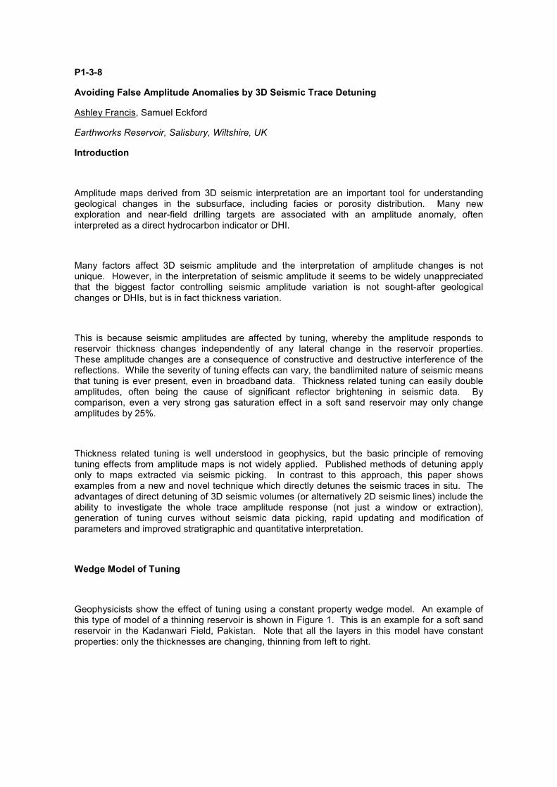
Figure 4 graphically compares the amplitude and thickness responses at well 14/10-4 and 14/10-5 before and after detuning. Before detuning (left panel) the downdip well 14/10-4 appears brighter than the updip well 14/10-5 despite having a lower net:gross. After detuning (right panel) the

orange tuning curve is now normalized to a constant level (green line) and amplitudes are proportionately rescaled as a function of thickness. The ratio of the blue dot to the green line is the same as before detuning (blue dot to orange line), but the detuned amplitude now correctly represents the relative change in net:gross between well 14/10-4 and well 14/10-5 and the higher net:gross well 14/10-5 now shows higher average amplitude.

Figure 4 left panel shows the computation of apparent seismic net:gross from amplitude. The ratio of the observed amplitude at a given thickness (blue dot) to the orange line at the same thickness is a measure of net:gross.

Ardmore Field, Central North Sea

Some of the advantages of the new seismic trace detuning method include faster and more reliable interpretation of amplitude anomalies. This is because the detuning method not only generates amplitude and detuned amplitude data, it also allows simultaneous direct computation of thickness and times of the amplitude events. This ensures that amplitude calculations are not in arbitrary windows, that may cut across events, and that only a single pick is required, rather than requiring a potentially time-consuming top and base zero-crossing pick to be made.

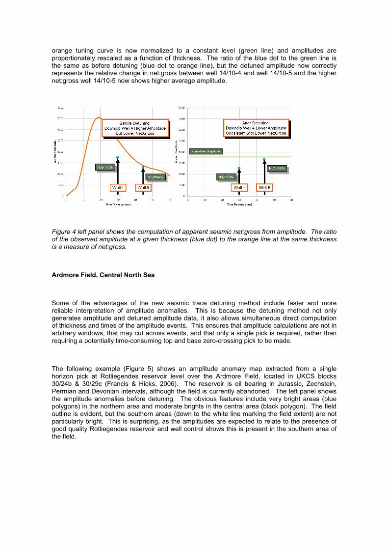
The following example (Figure 5) shows an amplitude anomaly map extracted from a single horizon pick at Rotliegendes reservoir level over the Ardmore Field, located in UKCS blocks 30/24b & 30/29c (Francis & Hicks, 2006). The reservoir is oil bearing in Jurassic, Zechstein, Permian and Devonian intervals, although the field is currently abandoned. The left panel shows the amplitude anomalies before detuning. The obvious features include very bright areas (blue polygons) in the northern area and moderate brights in the central area (black polygon). The field outline is evident, but the southern areas (down to the white line marking the field extent) are not particularly bright. This is surprising, as the amplitudes are expected to relate to the presence of good quality Rotliegendes reservoir and well control shows this is present in the southern area of the field.

Figure 5 Amplitude anomalies over the Ardmore Field at Rotliegendes level. Before detuning left) and after detuning (right)

The amplitude map after detuning is shown in the right panel of Figure 5. There are significant changes to the amplitude distribution. With detuning the field outline is much more sharply defined, and there is clear closure separation in the north-eastern corner of the field. The detuned amplitude response conforms nicely to the structural closure, unlike the original amplitude map. The very bright areas (marked with blue polygons) are de-emphasised and no longer conform to the previous polygons. The bright central area is now not bright (black polygon) and is simply consistent in indicating the presence of Rotliegendes reservoir all the way into the southern area of the field, as drilled in the wells.

York and Greater York, Blocks 47/2 & 47/3, UKCS

The York Field and the Greater York area comprise UKCS southern gas basin fields and potential near field targets. The area also includes the Rough gas storage field. Gas is present in both Rotliegendes and Carboniferous reservoirs; the presence of gas is known to brighten seismic amplitudes. The reservoir intervals are separated by a non-reservoir interval, which varies in being able to be resolved on seismic. An example relative acoustic impedance section is shown in Figure 6.

Figure 6 Relative AI section, Rotleigendes and Carboniferous reservoir intervals (green colours) below Zechstein (strong purple). Here the two intervals are separately resolved.

DT-AMP detuning was applied to the seismic and automated, entirely self-consistent attributes were extracted using the existing interpretation pick. The before and after detuning maps are shown in Figure 7 below.

Figure 7 Original amplitude map (left) and detuned amplitude map (right)

The impact of detuning is clearly evident. Before detuning, the most significant bright events are in the western Greater York area and the York and Rough Fields show comparatively little amplitude brightness. After detuning, the central and easterly known field areas are clearly bright and the western area appears less prospective. The brightness to the west is due to the thinner interval present, resulting in significant tuning. The Greater York area has since been relinquished by all partners.

Shallow Gas – Hazard or Resource?

The final example presented is taken from Netherlands block F09. Here, shallow gas is present and may be either a drilling hazard, or a potential resource. Amplitude analysis is frequently used for attempting to identify gas hazards, but of course tuning is still the predominant amplitude driver, so removal of tuning effects improves the reliability of amplitude analysis for gas hazards.

For shallow gas as a resource, a common criterion is to compare the conformance of the DHI to the structure. This is usually empirical and ad hoc, little more than overlaying structural contours on an amplitude anomaly map. A better approach is to measure the conformance of the closure to the amplitude anomaly. Technically this is a comparison of two binary indicator maps representing respectively the closure extent and the amplitude anomaly. These can be compared using the criteria in the following table:

Closure Amplitude Closure Binary

Amplitude Binary

Description Abbreviation

In Closure In Anomaly 1 1 True Positive TP

Not in Closure

In Anomaly 1 0 False Negative FN

In Closure Not in Anomaly

0 1 False Positive FP

Not in Closure

Not in Anomaly

0 0 True Negative TN

There are a number of available statistical descriptions for this comparison, the most appropriate being either the Matthew’s Correlation coefficient (MCC) or the F1 score. Both of these have a range from -1 to +1 and can be considered like a conventional correlation coefficient. However, in their usual published forms both these statistics scale and are hence relative, so a normalization is performed to make them absolute measures.

Conclusions

The effect of tuning on seismic amplitudes is widely recognized as an important effect but is rarely corrected for. In particular, there is a lack of awareness that thickness related tuning is the predominant physical effect controlling amplitude and that it can double the apparent amplitude of a seismic reflection. Because of this, all seismic amplitude data should be detuned before use. Detuning seismic data removes the most significant risk factor from the interpretation and makes amplitudes more easily interpretable in terms of geological criteria. Considering all the examples shown in this paper, it is clear that detuning is highly applicable to both lithological and fluid driven amplitude effects.

Seismic amplitude detuning is a self-consistent calculation and does not require external calibration such as well control. The use of 3D seismic detuning extends current map based approaches to detuning of seismic traces in situ in 2D lines or 3D volumes. This facilitates before and after detuning comparisons directly on seismic sections, before picking or further analysis. Detuning directly on the traces is significantly faster as it avoids the picking phase in both tuning curve analysis and interpretation. It also creates additional attributes which enhance the amplitude interpretation and ensure self-consistency.

References

Connolly, P., 2007, A simple, robust algorithm for seismic net pay estimation, The Leading Edge, October 2007.

Francis, A.M. and Hicks, G.J, 2006, Porosity and Shale Volume Estimation for the Ardmore Field using Extended Elastic Impedance. 68th EAGE Conference, Vienna, Austria

Francis, A.M., and Syed, F.H., 2001, Application of Relative Acoustic Impedance Inversion to Constrain Extent of E Sand Reservoir on Kadanwari Field, SPE / PAPG Annual Technical Conference, 7-8 November 2001, Islamabad, Pakistan

Acknowledgements

We are grateful to Rockhopper Exploration Ltd and Premier Oil PLC for permission to show images from the Sea Lion Field. We are grateful to Centrica PLC for permission to show images from the York and Greater York area. The Kadanwari example was originally released by LASMO and the Netherlands shallow gas example was worked up with assistance and guidance from EBN. The Ardmore data was originally provided by Acorn Oil & Gas Ltd.