p- and s-wave reflections from anomalies in the lowermost mantle

Geophys. J . Int. (1YY3) 115, 183-210

P- and S-wave reflections from anomalies in the lowermost mantle

M. Weber Seismologisches Zentralobseruaiorium GRF, Krankenhausstrasse 1-3, D-9 1054 Erlangen Germany

Accepted 1993 March 4. Received 1993 March 2; in original form 1992 September 17

S U M M A R Y Seismic P and S waves recorded at the G R F array in Germany are used to study the inhomogeneous structure of the boundary layer D" at the base of the mantle. The use of the seismic array allows the detection of small-scale anomalies in the lowermost mantle. The lateral resolution attainable is about 100 to 400 km, i.e. more than 10 times better than with tomographic methods.

The analysis of 13 years of G R F broad-band array data yields 255 events with high signal-to-noise ratio which are used to map the lowermost mantle. 74 of these events show anomalous P waves (PdP) which arrive 3-6 s after the direct P wave and have a slowness 0.7-0.8s/" smaller than the slowness of direct P. Other events close to the events with PdP do not have such an anomalous phase.

Using slowness, traveltime, amplitude and waveform information it is demonstrated that PdP is caused by an anomalous lower mantle velocity structure below the turning point of the P wave. If the pP phase (i.e. a P wave first reflected at the free surface near the source) is used together with the P phase, distinct and well-separated P-velocity anomalies can be determined under the Nansen Basin, the Kara Sea and northern Siberia. The areas of the bounce points of PdP in the lower mantle have a lateral extension of about 100 by 200 km, but this is not the size of the anomaly, since the resolution of P waves at 1 Hz in this depth is 130 km by 260 km (Fresnel zone). The accuracy to which the depth of the reflector (2612 km under the Nansen Basin and 2605 km under northern Siberia respectively) can be determined for l-D models is f 1 0 to 20km. The velocity contrast at the lower mantle discontinuity is about 3 per cent f l to 1.5 per cent. Areas which have velocity fluctuations smaller than about 1 per cent can not be detected as anomalous areas. 2-D models of the anomalies reveal the range of adequate models and possible trade-offs. If the lateral extension of the anomaly is about 7" the reflector has to be 40 km deeper than in the l-D model. If the dip of the reflector in the lowermost mantle is only about 1.5" it is difficult to resolve if the reflector is tilted towards the source or towards the receiver. For the anomaly under the Nansen Basin deviations from the great circle path are observed for PdP, indicating 3-D effects. Below the three anomalies the core-mantle boundary (CMB) can be located by PcP with a depth in agreement with standard earth models.

The analysis of the S waves (S, SdS and ScS) reveals two S-velocity anomalies in the lowermost mantle under northern Siberia. The first anomaly coincides with the P velocity anomaly under northern Siberia and can be explained by a 1-D model with a reflector depth of 2610 km f 15 km and a velocity contrast of 2.3 per cent. The second S-velocity anomaly is in an area where no P-velocity anomaly can be detected. The corresponding l-D S-velocity model has a reflector depth of 2575 km f 15 km and an S-velocity contrast of 2.6 per cent. The smallest structures that can be resolved with the S waves in this depth are about twice as large as for the P waves, i.e. 230 km by 460 km (Fresnel zone).

The joint analysis of P and S waves therefore shows a region with a P-velocity anomaly together with weak indications for an S-velocity anomaly (Nansen Basin) and a second region with a P but no S anomaly (Kara Sea). The lowermost mantle

183

Dow

nloaded from https://academ

ic.oup.com/gji/article/115/1/183/604140 by guest on 06 D

ecember 2021

184 M. Weber

under northern Siberia has a region where P - and S-velocity anomalies coincide, but also a region where only an S-velocity anomaly but no P-velocity anomaly is observed. This results in changes of the Poisson ratio from +5.9 per cent to -4.8 per cent ( f1 .5 per cent) across the discontinuity in the lowermost mantle for the regions studied.

Key words: body waves, D", core-mantle boundary, lateral inhomogeneities, lower mantle structure, Poisson ratio.

1 INTRODUCTION

The knowledge of the structure of the core-mantle transition zone is of crucial importance for the understanding of the dynamic behaviour of the Earth, since this region at the base of the mantle plays a vital role for processes like mantle convection, hot-spot plume generation and core cooling. Furthermore, it is the region with the strongest velocity and density contrast within the Earth (at the CMB), and it contains inhomogeneities on scale lengths from tens to thousands of kilometres.

The first to study this region, now generally called D" (Bullen 1950), was Gutenberg (1914), who determined the depth of the CMB and found that the velocity gradient in this region is different from the gradients above it, whereas Dahm (1934) postulated a discontinuity in the core-mantle transition zone. The global tomographic inversion of P and S traveltimes (see e.g. Dziewonski 1984; Dziewonski & Woodhouse 1987; Tanimoto 1987, 1990; Inoue et al. 1990) gives laterally varying velocities in the lower mantle, and the stochastic analysis of P and S traveltimes shows relatively large perturbations in D" (Gudmundsson, Davies & Clayton 1990; Gudmundsson & Clayton 1991; Davies, Gud- mundsson & Clayton 1992).

One of the major disadvantages of tomographic studies is the limited lateral resolution of about 60" in the lower mantle (Pulliam & Johnson 1992). This means that velocity anomalies smaller than about 4000km in D" can not be resolved with tomographic methods. One way to detect small-scale features in D" (dimensions of 100 to 400 km are found in the numerical modelling of convection) is the use of seismic arrays and networks. Since the study of high-quality regional data sets will not smear out the small-scale features compared to the use of global data sets in tomography, anomalous features with dimensions of a few hundred kilometres can be detected. Therefore the study of seismic records observed at seismic arrays and networks allows a resolution which can be about 10 times better than that of tomographic methods. Due to the lack of global coverage with seismic arrays, only a limited number of regions in the core-mantle boundary transition zone can be analysed, but the results derived for these regions can give a valuable set of complementary information extending the resolution of tomographic studies to smaller dimensions.

Long-period S-wave observations (Lay & Helmberger 1983; Young & Lay 1987) indicate a discontinuity in D" in the S-wave velocity, whereas Cormier (1985), Schlitten- hardt, Schweitzer & Miiller (1985) and Haddon & Buchbinder (1986, 1987) present evidence against such a

discontinuity. More recent work with S-wave data favour S-velocity anomalies in the lower mantle with typical lateral extensions of about 1500 km or smaller (Lavely, Forsyth & Friedemann 1986; Garnero, Helmberger & Engen 1988; Schweitzer 1990; Weber & Davis 1990; Young & Lay 1990; Gaherty & Lay 1992; Wysession, Okal & Bina 1992). See also Lay (1989) for a review.

Evidence for laterally varying P-velocity structure in the lowermost mantle was given in studies of short-period P waves by Vinnik, Lukk & Nikolaev (1972), Wright & Cleary (1972), Wright (1973), Wright & Lyons (1980), Ruff & Lettvin (1984), Wright, Muirhead & Dixon (1989, Schlittenhardt (1986), Doornbos, Spiliopoulos & Stacey (1986), Young & Lay (1989), Baumgardt (1989), Neuberg & Wahr (1991), Houard & Nataf (1992, 1993) and Vidale & Benz (1993), and by the use of long-period P waves by Wysession & Okal (1989), Hock (1992) and Wysession et al. (1992). Haddon & Cleary (1974), Doornbos (1978), Haddon (1982), Menke (1986a,b) and Bataille & Flattk (1988) present evidence for scattering that can be produced by CMB topography or velocity variations in D" [see also Bataille, Wu & Flattk (1990) for a review]. Further discussions on the influence of topography of the CMB on the wavefield are given in Creager & Jordan (1986), Doornbos (1988), Kampfmann & Muller (1989), Doornbos & Hilton (1989) and Neuberg & Wahr (1991).

Previous studies of P waves recorded at the GRF array [Davis & Weber 1990; Weber & Davis 1990 (WD)] show a prominent anomalous phase ( P d P ) in the P coda from events in the Northwest Pacific which is produced by reflection from small-scale P-velocity anomalies below northern Siberia. This anomaly was recently confirmed and its further extension analysed by Houard & Nataf (1992, 1993). A search for this anomalous phase in the Bulletins of the International Seismological Center (Weber & Kornig 1990, 1992) also shows this anomaly and indicates 10 other regions as promising to contain P-velocity anomalies.

Causes for anomalous structure of the D" zone can be manyfold and are the topic of controversy. Results of mineral physics, geochemistry and geodynamics suggest the following mechanisms: a chemically inhomogeneous boundary layer (Bullen 1949); a thermal boundary layer (Elsasser, Olson & Marsh 1979); subduction and accumulation of oceanic crust at the base of the mantle (Silver, Carlson & Olson 1988; Christensen 1989); convective thermal boundary layers with plume formation (Olson er al. 1987); chemical inhomogeneities through entrainment and lateral sweeping of D" material (Davies & Gurnis 1986; Ahrens & Hager 1987; Christensen 1987; Zhang & Yuen 1987, 1988;

Dow



ecember 2021

Anomalies in the lowermost mantle 185

Sleep 1988); a combined thermal and chemical boundary layer (Hansen & Yuen 1988, 1989); isobaric phase change due to strong lateral temperature gradients in D" (Anderson 1987); small-scale convection in D" and compositional plumes (Schubert et af. 1987); a boundary-layer instability and formation of thermal plumes (Yuen & Peltier 1980; Loper & Stacey 1983; Stacey & Loper 1983; Loper & McCartney 1986; Bercovici, Schubert & Glatzmaier 1989); reaction of perovskite (mantle material) with liquid iron (core material) forming chemical inhomogeneities (Knittle & Jeanloz 1989, 1991) [whereas recent work by Stixrude & Bukowinski (1992) suggests, that melting of perovskite does not occur in D"]. Since for example the melting point of iron under lower mantle conditions is currently a matter of active debate (see e.g. Ross, Young & Grover 1990; Boehler, von Bargen & Chopelas 1990; Boehler 1992) the discussion on the actual composition of the material in the core-mantle transition zone seems to be far from settled.

The aim of this seismological study, which started with the work described in Davis & Weber (1990) and Weber & Davis (1990), is to detect and locate small-scale P- and S-velocity anomalies at the base of the mantle with a seismic array.

2 P W A V E S

2.1 Observations

The earthquakes used in this study have distances from the GRF broad-band array that range from 66.9" to 87.5", but the majority of the events are at a distance between 70" and 80". The body wave magnitude, ml,, is between 5.0 and 6.7 and the source depths h are between 5 and 645 km. 255 events with high signal-to-noise ratio satisfying these conditions were recorded between 1978 and 1990 and are listed in the Appendix, sorted by backazimuth (BAZ). The events already used in WD are underlined. The source parameters are from PDE. The borderline cases have energy in the appropriate time-backazimuth-slowness window but insufficient data quality for a definite identification. 74 events have PdP, 120 have good signal-to-noise conditions but no PdP, and 61 are borderline cases. The equivalent numbers in WD are 10, 10 and 4, respectively. Fig. l(top) gives the distribution of the events studied.

WD contains a detailed discussion proposing that the anomalous phase PdP, which arrives after P with a time delay of 3 to 6 s and a slowness ul,dl, 0.7 to 0.8s/" smaller than that of P , is produced by a reflection from a lower mantle discontinuity below the turning point of the P phase. PdP is an anomalous phase in the sense that it can not be explained by standard earth models. The fact that the events without PdP are close to events with PdP opens the opportunity to map the 'anomalous' lower mantle. To demonstrate that the slowness, a measure of the angle of incidence of the wave at the array, plays a crucial role in the identification of PdP we show in Fig. l(bottom) rays with the slowness u of P ( fO. l s / O ) , PdP (ul+,/,- up = -0.7s/") and PcP (upcp - ul, = -1.3 s / O ) , which are traced back from GRF towards the source region. Take-off angles at GRF are determined from the observed slowness, corrected for effects from the underground below the array (Kriiger &

nI5TANCE I O E G l

N

P

1 - -20 0 20 40 60 80 100

, . l ' I ' l ' I

Figure 1. (Top) Geographical distribution of the 255 events studied (stars) and the location of the GRF array (triangle). The lower mantle turning/reflection points of the waves from the events to GRF are indicated by circles. The projection used is azimuthal equidistant with GKF as the projection pole. (Bottom) Paths of rays for P, PdP and PcP starting at GRF (triangle at 77" distance) traced back to the subduction zone indicated by the star. The velocity model used is the PWDK model (WD) and the Earth-Flattening Approximation (EFA, see e .g . Miiller, 1977) has been applied. The CMB and the discontinuity of PWDK in the lower mantle are also indicated.

Weber 1992). In Fig.1 (bottom) the model of WD with a discontinuity in the lower mantle is used. A11 three phases end in the source region indicated by the star. If no reflector in the lower mantle below the turning point of P would be present, the rays with the PdP slowness would end more than 1000 km to the left of the source region (see Fig. 7 in WD). This shows that the use of an array is of crucial importance, since it allows the determination of the slowness of the phases and therefore the depth of the penetration of a wave. Fig. l(bottom) also demonstrates that effects in the source region like slab effects, see e.g. Vidale (1987), Cormier (1989) and Vidale, Williams & Houston (1991), can be ruled out as producing PdP since such phases have almost the same slowness as P.

Due to limited space the analysis of the 255 events can not be presented, but Fig. 2(top) shows one example with PdP and PcP, i.e. of phases which have a slowness 0.8s/" and about 1.4s/" smaller than that of P (event 94). Also given in

Dow



ecember 2021

186 M. Weber

136

11% IN 5

I kit d

f "f

59 PdP N 46 PcP N C Y C L E S N I CYtLESmM

n! "9'" 0 ' -galg ' 0

0 7

0 ?

I d d

J L

E E Figure 2. Vespagrams and FK spectra for events from the Appendix (number at upper right) for the vertical components filtered with a WWSSN-SP filter. The contour interval for the isolines is -3 dB in all figures. (Top) Four vespagrams with time segments 15 s long (20s for event 178) and a slowness window from 3 to 7s/'. The first onset is P ( p P for event 178) and the seismogram below each vespagrarn is the corresponding P beam (the pP beam for event 178). The dashed box for event 178 outlines the expected time-slowness range for pPdP. (Bottom) Two FK spectra of the PdP and PcP phase in the k , - k, (east-north) plane for the frequencyf = 1 Hz respectively. The slowness of the phase is given in s/o by u = 111.19 Ik(/(2nf). The full diamond is the value for the corresponding P phase of the event. The dashed line gives the backazimuth of P and the full line the backazimuth of PdP or PcP.

Dow



ecember 2021


(a) NANSEN BASIN

I

(b)KARA SEA + NORTHERN SIBERIA

Figure 3. (a) Geographical distribution of bounce points of PdP from earthquakes in the Aleutian Islands (number 11 to 68) on a discontinuity in the lowermost mantle under the Nansen Basin. The North Pole is indicated by a cross. For five events vespagrams are shown. All vespagrams have time segments that are 15 s long and a slowness window from 3 to 7s/" [see Fig. 2 (top) for more details and large plots of vespagrams]. Full circles indicate bounce points with PdP. The size of the circles is proportional to the energy of PdP with respect to P (see scale). Open circles denote bounce points which show no PdP. Diamonds are the bounce points for borderline cases. The projection is centred on (86N, 95 E). See smaller map for location of this area and of GRF (triangle). The bounce points have been projected to the Earth surface together with the axes of the effective Fresnel zone ellipse (2" by 4"). (b) As Fig. 3(a) but for the bounce points of PdP from earthquakes in Kamchatka, the Kuriles and Japan (number 69 to 224). The area shown covers the Kara Sea (75 N, 84 E) and northern Siberia (72 N, 86 E) and is centred o n (75 N, 85 E).

Fig. 2(top) is a borderline case (event 80) and an event without PdP or PcP (number 136). For more examples, see WD and Fig. 3. At the bottom of Fig. 2 frequency- wavenumber (FK) spectra (for details see e.g. Hanka & Seidl 1986) are given. FK spectra give energy as a function of backazimuth and slowness. The backazimuth of the

phase is measured from north. The reduced slowness of PdP with respect to P can be seen by the smaller radius of the PdP energy maximum from the centre compared to the radius for P. PcP (event 46) and most observations of PdP have the same back-azimuth as the P wave. Only for a few of the Aleutian events does the observed backazimuth of the PdP phase deviate from that of the P wave [event 59 in Fig. 2(bottom) and event 62 in Fig. 131. A more detailed discussion of this deviation in backazimuth will be given later, but it should already be pointed out here, that the accuracy of the backazimuth determination, defined by the size of the first contour line in the spectrogram, is of the same order of magnitude as the deviations from the P backazimuth.

2.2 Distribution of bounce points in the lower mantle

Fig. 3(a) gives the distribution of bounce points of PdP from earthquakes in the Aleutian Islands on a discontinuity in the lowermost mantle under the Nansen Basin. Event 12 in Fig. 3(a) does not show PdP and event 34 is a borderline case. The size of the effective Fresnel zone ellipse (2" by 4", i.e. 130 km by 260 km in the lowermost mantle), which is about half of the size of the classical (first) Fresnel zone, gives an indication of the lateral resolution which can be achieved in the lowermost mantle by P waves with a dominant frequency of 1 Hz.

WD found one event (number 19 in WD, now number 47) with PdP in this region. The 17 additional events with PdP presented here give some indication of the size of the anomaly at the base of the mantle under the Nansen Basin. The area covered by the cluster of full circles is 70 km by 160 km in the lower mantle, but this is not the extent of the anomaly. Since only GRF data and Aleutian events are used, the coverage is limited to this strip of about 70 km width in the lower mantle. Therefore, the extent of the anomaly to the left and right (West and East) of the cluster in Fig. 3(a) can not be determined with these data, whereas the maximum extent of the anomaly towards north and south can be given since the events occur along the whole island chain of the Aleutians [see Fig. l(top)]. Nevertheless, it should be kept in mind that features smaller than the Fresnel zone in Fig. 3(a) can not be resolved with these data.

Previous studies employed precursors of core phases (PKIKP) to detect anomalies in the lower mantle (see e.g. Doornbos & Vlaar 1973). The corresponding area with anomalies in the lower mantle is about lo" to the left of the cluster in Fig. 3(a) and the anomalies detected by Haddon (1982) are even further away. A better lateral resolution than with the Aleutian events can be achieved with events from Kamchatka, the Kuriles and Japan since these subduction zones have a larger lateral extension. This gives an area covered by bounce points in the lower mantle of up to 200 km width. Fig. 3(b) gives the bounce points of PdP on a reflector in 2605 km depth (PWDK). The area shown covers the Kara Sea and northern Siberia and is directly adjacent to the South (bottom) of Fig. 3(a).

The cluster of bounce points with PdP under the Kara Sea, event 100, 116 and 121, was not analysed previously. The size of this cluster in the lowermost mantle is about

Dow



ecember 2021

188 M. Weber

70 km by 150 km, but the limits of resolution indicated by the Fresnel zone ellipse in Fig. 3(a) should be kept in mind.

The conclusion from the data presented here is also in agreement with the results of Weber & Kornig [1992, Fig. 6(b)], where anomalous bins under the Kara Sea were found. Further north, i.e. in the area of the bounce point of event 75, no anomalous bins could be detected in Weber & Kornig (1992). That the lower mantle anomaly under the Kara Sea extends further to the West (left) and north-west is demonstrated in Houard & Nataf (1992, 1993). In these studies events recorded at the L D G network in France are used to detect PdP. The fact that for three events PdP is observed at L D G but not at G R F is an additional indication that a lower mantle anomaly produces this phase, since a phase due to a source effect would be observed at both arrays.

South of the Kara Sea cluster a region of about 70km width in the lower mantle with bounce points without PdP can be detected. The vespagrams of a deep event (event 136, h =499km) and of a shallow event (event 138, h = 79 km) with bounce points in this region are shown in Figs 2 and 3(b). The fact that open circles (no PdP observed) are very close to full circles ( P d P observed) suggests that strong lateral changes in the lowermost mantle occur. The WWSSN-SP filtered seismograms from the NARS array used in W D also did not show PdP in this area. With the enlarged data set presented here it is now possible to locate this gap with increased accuracy.

Further south the largest of the three clusters of P d P bounce points [see e.g. event 166 and 196 in Fig. 3(b)] can be detected under northern Siberia. The lateral extension of this cluster previously reported in W D is 100 km by 200 km in the lowermost mantle. The addition of 25 events with PdP allows a much better coverage and determination of the extension of this cluster. The determination of the limits of this cluster towards the south is now possible with events under Japan, see e.g. number 203 in Fig. 3(b). The bounce points of these events yield the open circles south of the northern Siberia cluster. That the lowermost mantle south of the bounce point of event 203 does not contain P-velocity anomalies was already shown in Schlittenhardt (1986).

Since the radiation patterns of the events considered here (see Appendix) vary very much along the strike of the subduction zones and also in the downdip direction (see e.g. Zhou 1990) the negative observations of P d P are not due to poor radiation in the direction of D".

Spies (1991) reports that the AB-branch of P K P of Tonga-Fiji events recorded at G R F is delayed with respect to the other branches of PKP. This effect could be produced by the anomalous lower mantle under the Kara Sea and northern Siberia, since only the AB-branch travels through the area of these clusters on its way from the CMB to the receivers. The bulletin analysis in Weber & Kornig (1992) is in agreement with the results from the observations at G R F , since it also shows anomalous bins in this area.

Events in the North Pacific Ocean, which would have bounce points to the east (right) of the clusters shown in Fig. 3, are very rare (see e.g. Wysession, Okal & Miller 1991), therefore G R F data d o not offer the possibility to cover this region. The area west of the clusters can not be analysed with the P wave and its coda, since the seismicity of the subduction zones ends at about 650 km depth. A n approach

to extend the coverage towards the west, i.e. towards the G R F array, is given in the next section.

2.3 The depth phasepP

The coverage of the anomalies in the lowermost mantle can be extended if the depth phase pP and its coda is used. The bounce point of pPdP, i.e. of the phase reflected at the surface and then on a lower mantle discontinuity, is shifted towards the receiver by up to 2.5" (170 km in the lowermost mantle) with respect to the corresponding P d P bounce point. Another advantage of the pP phase is that this wave leaves the subduction zone almost perpendicular to the slab and does not travel in the penetration direction of the slab.

The pP wave is usually more complex than the P signal due to multiples from the sedimentary layers and back-arc basins which will give additional energy in the pP coda (see e.g. Engdahl & Kind 1986, Wiens 1987 and Schenk, Muller & Brustle 1989). Therefore the slowness analysis is again the key to separate pPdP from other energy in the pP coda. The delay time Atp,~d,,+,,~ will not be used to determine the depth of the reflector in the lower mantle since the paths of pP and pPdP towards the surface are different and therefore the difference traveltime of the pP and the pPdP phase might vary by up to about f 2 s (see dashed box in Fig. 2 for event 178, which is 4 s wide).

In Fig. 4(top) the distribution of bounce points of p P d P is given. Event 23 confirms the results given in Fig. 3(a), i.e. no energy is reflected in the lower mantle close to the North Pole. Events 36, 53 and 180 are borderline cases. For event 178 (number 11 in WD) PdP is observed, but pPdP is absent (see Fig. 2), i.e. the area of the lower mantle acting as a reflector is limited towards West. This observation is confirmed by the three additional events giving open squares in the same area in Fig. 4(top). Event 188 (number 8 in WD) shows pPdP.

The conclusion from the study of the depth phase pP is that the P-velocity anomaly under northern Siberia does not extend to the west. The Fresnel zones of PdP (full circles) are sufficiently separated from the Fresnel zones of the four events without pPdP (open squares) to give confidence in this result.

2.4 Reflections from the core-mantle boundary

The next step after localizing P-velocity anomalies in the lower mantle is to determine the core-mantle boundary structure below these anomalies. The distribution of the bounce points of P c P is shown in Fig. 4(bottom). For event 46 and event 94 vespagrams/FK spectra are shown in Figs 2 and 3(a). Fig. 4(bottom) also gives the effective Fresnel zone ellipse of PcP for waves with a frequency of 1 Hz with axes which are almost 50 per cent larger than those of PdP, i.e. 2.7" by 5.5". For details on the Fresnel zone of PcP see Kampfmann & Muller (1989).

Since PcP has a small amplitude with respect to P in this distance range (see next section for synthetic seismograms), favourable conditions (good signal-to-noise ratio and good PcP radiation) are necessary for the observation of PcP. The areas in Fig. 4(bottom) with reliabie P c P observations (i.e. events 46, 94, 145 and 152) coincide with the areas where PdP is observed.

Dow



ecember 2021


NANSEN BASIN + KARA SEA + NORTHERN SIBERIA

+" [III1-----23

pPdP

0

I pc p :P

.

+"

0 b 7 0 . 8 8

0 b 5 0 . 1 9

0 B35.5e

0 ) 2 5 . 1 8

j 1 7 . 8 8

b 1 2 . 6 1

0 b 8 .98 . ) 6 . 3 e

0 b 7 0 . 8 8

0 b 5 0 . 1 1

0 b35.58

0 b 2 5 . 1 1

0 B17.88

Figure 4. (Top) Geographical distribution of bounce points of pPdP under the Nansen Basin, the Kara Sea and northern Siberia. For event 178 the pP vespagram is given in Fig. 2 (top). Open squares denote bounce points which show no p P d P , full squares indicate bounce points with pPdP, diamonds are the bounce points for borderline cases. The full circles are the bounce points with PdP given in Fig. 3 . The projection is centred on (80N, 90E). The effective Fresnel zone ellipse of p P d P is 2" by 4". (Bottom) Geographical distribution of the bounce points of PcP. Large stars are reliable PcP observations (see Fig. 2 for event 46 and 94), small stars stand for bounce points which give energy in the appropriate time-slowness-backazimuth window of PcP, but with insufficient data quality. The full circles are the bounce points with PdP given in Fig. 3 . The effective Fresnel zone ellipse of PcP is 2.7" by 5.5".

In conclusion, reflections from the CMB under the anomalies below the Nansen Basin, the Kara Sea and northern Siberia can be detected. The discussion in the next section will show that the time delay Atpcl,-l, is in agreement with the values derived for standard earth models, i.e. the CMB under the three lower mantle P-velocity anomalies given here does not show an anomalous behaviour.

2.5 1-D models

Before 2-D models of the P-velocity anomalies in the lowermost mantle are tested, 1-D P-velocity models for the areas under the Nansen Basin, the Kara Sea and northern Siberia are presented in this section.

The P-velocity models PWDK and PNAN are given in Fig. 5(a). PWDK is the model for the lowermost mantle under the Kara Sea and northern Siberia (see Fig. 3b) and PNAN is the model for the lowermost mantle under the Nansen Basin (see Fig. 3a). The velocity model PWDK (PNAN) is derived by fitting the theoretical delay times AtFyD_K;!PNAN) of PdP with respect to P to the observed defay times Atz; - , . . The same procedure was also applied to the PcP phase. The model PWDK (PNAN) is the optimum model found, i.e. AT = At;&!7$PNAN) - Atdata I W l ' - I'

for PdP and similarly for PcP is a minimum. To show how accurate the depth and the velocity contrast

at the discontinuity in the lower mantle can be resolved, the effects of modifications of the PWDK and PNAN models on the traveltimes and the amplitudes are presented.

2.5.1 Traveltime information

Figure 5(b) gives the P velocity of model PWDK together with three other models which vary by f 5 km in depth and f 0 . 5 per cent in velocity contrast from PWDK respectively. The resulting traveltime residuals for PdP and PcP as a function of source-receiver distance are given in Figs 5(c) and (d), respectively, together with data for a few of the Kurile events. Stars with error bars are the residuals AT of the observed delay times with respect to the PWDK model. The observed delay time is the time difference between the maxima of the isolines for PdP and P in the vespagrams. The error bar is the sum of the width (diameter) of the first isoline (-3dB from the maximum) for the P and the PdP energy. As can be seen in Fig. 5(c) the fit between PWDK and the data is good for deep events (number 178, h = 622 km) and for shallow events (number 189, h = 50 km) indicating that PWDK is an adequate model. The same holds true for the P c P results in Fig. 5(d).

The full circles, open circles and semi-full circles are the traveltime residuals for the three models shown in Fig. 5(b) with respect to PWDK (i.e. A T = AtFzF7, - A t ~ ~ ~ ~ l J ) and similarly for PcP. Increasing the depth of the reflector by 5 km (open circle) shifts the traveltime residuals of PdP by about -0.2s, since the P d P path becomes longer, and a similar effect is observed for PcP. The opposite effect for PdP is achieved if the velocity contrast is reduced by 0.5 per cent (full circle) since then the velocity above the discontinuity is increased. The traveltime of PcP is almost unaffected since the velocity below the discontinuity is decreased in this model.

A major problem in determining the best 1-D model is the trade-off of the traveltime effects between the depth of the reflector and the velocity contrast. To illustrate this effect the semi-full circle gives the delay times for a model where the reflector was raised by 5 km and the contrast increased by 0.5 per cent. Whereas the effects of these two changes to PWDK almost compensates in PdP, the effects in PcP do not compensate. Therefore, only the use of PdP

Dow



ecember 2021

I90 M . Weber

2700- PNAN

2800 -

7 3.2 13.6 14.0

2200

2300

2400

L 4 2500

s: L 2600

Q 2700

s

9

2800

P VELOCITY ( K M / S )

?

I I

13 2 13.6 1 '

P VELOCITY f K M / S ) 3

-. 0 8

2 0.6

2 0.4

n 0.2

0.0

0

v

3

w : -0.2 A w -0.4 > 6 2 -0.6

t 178 4 I / T

fi 189 /

1 -0.8 1 -1.01 " " ' I " " " ' 1 74.0 75 o 76.0 77.0 78.0 79.0 80.0 81.0

Figure 5. (a) P velocity of model PWDK (depth of discontinuity hrcn = 2605 km, velocity contrast Av,, = 3.0 per cent) and of model PNAN (h,efl = 2612 km, Av,, = 3.0 per cent) in the lowermost mantle under the Kara Sea/northern Siberia and the Nansen Basin respectively. Three standard earth models [JB (Jeffreys & Bullen 1940). PREM (Dziewonski & Anderson 1984) and IASP91 (Kennett & Engdahl 1991)] are also given and the CMB is indicated. (b) P velocity of model PWDK (full line). The three other models have the following parameters: hrcR = 2605 km, AvP = 2.5 per cent (full circle); hrCn = 2610 km, Au,, = 3.0 per cent (open circle); hrcn = 2fN0 km, A u p = 3.5 per cent (semi-full circle). (c) Traveltime residuals for PdP as a function of source-receiver distance. Stars with error bars are the traveltime residuals AT of the observed delay times (data) with respect to the PWDK model, i.e. AT = AtFy:: - At$;;-1x. The full circles, open circles and semi-full circles are the traveltime residuals for the three models shown in Fig. 5(b) with respect to PWDK, i.e. AT = A r ~ ~ ~ ~ , - A f ~ ~ ; ~ p (d) As Fig. 5(c) but for PcP.

together with the analysis of PcP allows some control on this trade-off.

Another problem in determining the best velocity model is that the source depth and the epicentre of the events are known only with a certain accuracy. The length of the mislocation vectors for the epicentres of events in the Kuriles, with turning points under the Kara Sea and northern Siberia, is of the order of 0.1" (see e.g. Kennett & Engdahl 1991). This slight increase in source-receiver distance reduces the theoretical delay time of PdP with respect to P by about 0.1 s.

The conclusion that can be drawn from the modelling and fitting of traveltimes presented here is that the depth of the

discontinuity and the velocity contrast can be determined with an accuracy of up to f5 km to 10 km and f0 .5 to 1.0 per cent respectively.

A similar trade-off between reflector depth and P velocity above the discontinuity exists for PcP and the CMB. Here a reduction of the velocity in the D" layer by 0.2 per cent can be compensated by raising the CMB by 9km, i.e. to 2889 km depth as in IASP91.

A complication in determining the velocity in the lower mantle under the Nansen Basin is that the Aleutian events show some of the largest mislocation vectors observed, see e.g. Engdahl & Gubbins (1987) and Kennett & Engdahl (1991). The mislocation reaches up to 0.4" with typical

Dow



ecember 2021


values of 0.2" to 0.3". Therefore the PNAN model (h,,,=2612 km, Av,,=3.0 per cent) can only be con- strained up to *10 km to 20 km in reflector depth and f l . O to 1.5 per cent in P-velocity contrast with the data presented here.

2.5.2 Fit of observed traveltimes to PWDK and PNAN

PWDK and PNAN are adequate models of the lowermost mantle under the Kara Sea, northern Siberia and the Nansen Basin respectively, since over 85 per cent of the 74 events with PdP have a delay time of PdP with respect to P that deviates 0.3 s or less from the delay time predicted by the corresponding lower mantle velocity model. If the residual AT = At::??,, - At$::-,, is negative this means that either P travels faster than predicted from the model or P d P is slower or a combination of both occurs.

Fir to PWDK. Fig. 6(a) shows the geographical distribution of epicentres of earthquakes in the Kurile Islands which show PdP (open circles). Only events with an accuracy in the delay time better than 0.7s are shown. As can be seen in Fig. 6(a) deep events (top left, source depth of 489 km and deeper) and shallow events (events close to the trench) fit the PWDK model very well. The only area where the residual is larger than 1.0s is in the dashed box for source depth of about 100 km. The three epicentres with residuals between - 1.1 and - 1.5 s are surrounded by events with little or no residual that have bounce points on the lower mantle discontinuity which are only 60 km apart. A syncline in the lower mantle reflector able to produce the residual of -1.5 s would therefore have to have a depth of 55 km and a lateral extension of less than 60 km. Since 60kilometres are only a quarter of the effective Fresnel zone, such a small-scale indentation in the reflector will not be visible due to the wavefront healing effects (see e.g. Emmerich 1991). Therefore, the most likely area where this residual is produced is the subduction zone.

A section through the subduction zone segment outlined by the dashed box in Fig. 6(a) is given in Fig. 7. The three events just mentioned are located in the area where the subduction zone changes its dip. To explain the observed delay it is sufficient that the P wave travels 100 to 300 km longer in the slab (higher velocity), or that PdP passes through slower material under the slab, o r that a combination of the two effects occurs. From the data available it is not possible to pin down the reason of this residual.

Since for the large majority of the data the fit of the observed delay time to the delay times of PWDK is very good, the PWDK model is an adequate 1-D model for the lowermost mantle under the Kara Sea and northern Siberia.

Fir to PNAN. Fig. 6(b) shows epicentres in the Aleutian Islands and the traveltime residuals with respect to the PNAN model. The maximum deviation from the traveltime delays predicted by the model are f0 .5 s. No strong systematic trend or clustering of residuals is visible, indicating that the PNAN model is an adequate 1-D model for the lowermost mantle under the Nansen Basin.

a - 1 . 5

@ -1.2 s

@ -0 .9 s

@ - 0 . 3 s

@ t0.3 s

@ -0.6 s

@ +0.6 s

KURILE ISLANDS

ALEUTIAN ISLANDS

2OOkrn b 4

Figure 6. (a) Geographical distribution of epicenters of events in the Kurile Islands with PdP (open circles). The size of the triangles in the circles is proportional to the traveltime residual A T = AtF;P_", - see scale. The projection used is orthographic, centred on (48 N, 153 E). The dashed box is the slab segment N5 in Zhou (1990). The arrow gives the direction towards GRF, and the trench is indicated. (b) As Fig. 6(a) but for the Aleutian Islands and the PNAN model. Map centred on (52 N, 177 E) .

2.5.3 Amplitude information

In Fig. 8 the effects of the thickness D of a transition zone and of the P-velocity contrast Av,, a t the discontinuity in the lower mantle on the amplitude of the PdP-wave group are shown. The model used is PWDK but similar conclusions can be drawn for the PNAN model.

Figures 8(a) and (b) give the P-velocity model PWDK together with six modifications, for which seismograms are computed with the reflectivity method (Fuchs & Muller 1971; Muller 1985). That the amplitude of PcP decrease with increasing distance whereas PdP increases with increasing distance can be seen in Figs 8(c) and (d), and the traveltime

Dow



ecember 2021

192 M. Weber

/ /

/ f

/ /

/

(-2;

V I 0 , 1 40

I 200 1

500 1 I s1615 (14) I

-157 (17) 164 (19)

-178 (20)

600 -

73 74 75 76 77 78 79 80

DISTANCE f D E G

Figure 7. Location of hypocentres in the slab segment N5 in Zhou (1990) (see dashed box in Fig. 6a) as a function of distance from GRF. The numbers of the earthquakes are as in the Appendix, and the numbers in brackets are the numbers of these events in Zhou (1990). Open circles are events for which IATI is smaller than 0.2s. The events 150, 156 and I60 (triangles), are given with their A T values in seconds. The dashed line indicates the subduction zone with a dip of 12" and 50", respectively. The full triangle at the top marks the location of the trench, and the two open triangles indicate the extent of the dashed box in Fig. 6(a).

curves are shown in Fig. 8(e). If the velocity jump at the discontinuity is smeared out (transition zone with a thickness D = 3A), P and PcP are unaffected, but the lack of a sharp discontinuity decreases the amplitude of the PdP wave group significantly.

To get a better understanding of this amplitude effect, Fig. 8(f) gives the ratio of the PdP amplitudes of the six alternative models with respect to the PdP amplitudes of PWDK. Smearing out the velocity contrast reduces the amplitudes for shorter distances drastically ( D = 2A to 4A), whereas the effect at larger distances is not so severe. Reducing the velocity contrast reduces the amplitudes of PdP at all distances by almost the same factor, i.e. to about 2/3, if the contrast is reduced from 3 to 2 per cent. Even for the events with the best signal-to-noise ratio, the amplitude information gives only a resolution of about f1.0 to 1.5 per cent in the velocity contrast Av,,, and the thickness D of a transition zone can not be resolved if D is smaller than 2A t o 3A. Fortunately the traveltimes are also affected by such model changes, so that these values are the resolution limits only if solely the amplitude information were used.

The discrimination between the two effects will eventually become possible, if a network of seismic stations of 5" to 10" length along a great circle path can be used, since the amplitude ratio is strongly dependent on the distance if the discontinuity is smeared out, whereas no strong amplitude ratio changes as a function of distance are produced by a reduction in the velocity contrast.

If the velocity contrast a t the discontinuity is smaller than about 1 per cent, even such a network of seismic stations will not help in detecting such anomalies (see also Schlittenhardt 1986, Fig. 13), since the amplitudes are then reduced too much. Therefore, velocity fluctuations smaller

than about 1 per cent at the base of the mantle will be difficult to map.

The final conclusion from the modelling of traveltimes together with the results derived from the modelling of amplitude effects, is that the I-D P-velocity model PWDK for the area under the Kara Sea and northern Siberia can be determined with an accuracy of about fS to 10 km in the reflector depth and f 0 . S to 1.0 per cent in the velocity contrast. The resolution for PNAN, i.e. for the P-velocity model for the lowermost mantle under the Nansen Basin, is f 1 0 t o 20 km and f l . O to 1.5 per cent.

2.6 2-D models

The method which is used for modelling the laterally inhomogeneous lower mantle is the Gaussian beam method (GBM) (Cerveng, Popov & PSenEik 1982; Popov 1982). The GBM produces the right type of waveform for the PdP wave group and the amplitudes of the PdP wave group and of P c P deviate less than 12 per cent from the exact values in the source-receiver distance range considered here. A more detailed discussion of the accuracy of the GBM in inhomogeneous media can e.g. be found in Weber (1988, 1990). The computing time for the GBM is SO0 times smaller than the computing time for the reflectivity method and facilitates interactive modelling of the 2-D structure of the lowermost mantle. The ray paths, traveltimes and synthetic seismograms for the 2-D models in this section are all computed with the GBM.

For a better comparison of the different models presented in this section, Fig. 9 gives the ray paths, traveltimes and synthetic seismograms of P, PDP, PdP and PcP for the PWDK model and event 189. The P D D P phase, i.e. a wave reflected at the underside of the discontinuity, is also included. Since PDDP arrives almost at the same time as P D P and has a very small amplitude in the distance range considered here, it is not denoted separately in Fig. 9. Event 189 corresponds to the data point with the largest distance to G R F (A = 79.2") in the modelling of PdP traveltimes in Fig. 5(c). Fig. 9(c) will serve as reference for the 2-D modelling, since PWDK is a 1-D model in agreement with the data observed at GRF.

Models with reduced lateral extension. A first step towards realistic 2-D models is the reduction of the lateral extension E of the lower mantle reflector to 2.5" without changing the reflector depth and the P-velocity contrast of PWDK. This anomaly, shown in Fig. l0(a), has an extension large enough to be sampled by all phases of the PdP-wave group as in the 1-D model PWDK. Therefore, the resulting seismograms (Fig. 10c, GRF at A = 0") for this model agree with the observations at GRF. The splitting of the PdP-wave group visible at A = -3" in Fig. lO(c) is due to the fact that PdP and PDP are at that distance almost I s apart, so that the two phases with a dominant period of 1 s are separated. PcP is for this model 0.6s too early, since it runs outside the low-velocity area (LVA) above the reflector. Reducing the contrast a t the discontinuity from 3.0 to 2.7 per cent by decreasing the velocity in the high-velocity area (HVA) below the reflector would give a good fit of PcP to the observations. Such a change in the HVA is well in the range of possible models.

Dow



ecember 2021


2700

2800

2900

-

-

-, , 1

2200 /b: I

2300 2400 2500 2600 2700

2800 2900

13.2 13.8 P VELOCITY (KM/S)

65O 75O *mO 65O

340 I 00 I

-

300.00 I

65' 75' A05'

E 1.0 2 4 0.8

2 0.6

0.4

5 4

T

68 72 76 80 DISTANCE ( D E C )

Figure 8. The effect of the thickness D of a transition zone and of the P-velocity contrast Au, in the lower mantle on the amplitudes of the PdP-wave group. The dominant period of the wave is 2 s and the wavelength 1 is 27 km. (a) P velocity of model PWDK (hren = 2605 km, Aup = 3.0 per cent) and of four models with transition zone thickness D equal to 1 to 41. (b) PWDK and two models with Aup = 1 per cent and 2 per cent at the discontinuity, respectively. (c) Seismogram section (displacement) of vertical components for PWDK for a source in 131 km depth. The seismograms are computed with the reflectivity method (Fuchs & Miiller 1971; Miiller 1985) for an isotropic point source and reduced with 5.0s/". (d) As Fig. 8(c) but for the model with D = 31. (e) Traveltimes of P, PDP, PdP and PcP. Distance-time frame and reduction velocity as in Fig. 8(c). (f) Amplitude ratio of the PdP-wave group for the six models in Figs 8(a) and (b) with respect to the P d P wave group for PWDK (full triangle) as a function of distance.

Dow



ecember 2021

194 M. Weber

24 30 36 42

336

334

$3?

%O

328

326

324

.oat\ 1

. 00 -4 -

40 54 60

>

-4 -2 0 2 A4 Figure 9. (a) Paths of rays from event 189 (distance A = 79.2") to GRF located at distance A = 0". The model used is PWDK (hrcfl = 2605 km, Aup = 3.0 per cent) and the EFA has been applied. The CMB and the discontinuity of PWDK in the lower mantle are indicated by solid lines. The intervals between the P-velocity isolines (dashed lines) are 0.5 km s- I . The two full triangles (A = 38.1" and 40.7") indicate the range of bounce points of PdP under northern Siberia. (b) Traveltimes of P, PDP, PdP and Pcp for PWDK in the region of the GRF array. The distance-time frame is centred on GRF (A = 0"). The reduction slowness is 5.0s/". (c) Seismogram section (displacement) of vertical components for PWDK in the area of the GRF array for event 189.

As was shown in the discussion of the depth phase p P [Fig. 4(top)] the anomaly under northern Siberia is limited towards the West, i.e. towards GRF. The limit of the reflector determined with p P is indicated by the full triangle in Fig. 10(b), and the corresponding seismograms are given in Fig. 10(d). Since the PdP-wave group encounters less of the LVA to the left of the reflector, the PdP-wave group is 0.35s too fast and this model does not explain the observations.

Before other models are presented it should be pointed out that the anomalies located with the observations at GRF are illuminated by energy travelling from the Northwest Pacific to central Europe. Since we do not have coverage from other azimuths, we cannot deduce a unique model of the lower mantle anomaly. Therefore, the following models only give some ideas of the possible range of velocity anomalies able to explain the observations at the GRF array. The aim in presenting these models is also to give some insight into possible trade-offs between different model parameters.

Models with reduced lateral extension and greater depth of the reflector. Fig. 11 shows a model for the anomaly under northern Siberia with small lateral extension ( E = 6.6"). The size of the reflector is derived by adding an effective Fresnel zone of 4" to the range between the two full triangles in Fig. 9(a). It should be pointed out, however, that this value of 6.6" is not necessarily the minimum size of the anomaly but rather the minimum size resolvable with 1 Hz P waves and GRF data. In Fig. 11 Au,, = 3.0 per cent in both models, but hr,,=2605km in Fig. l l (a ) and 2645 km in Fig. l l(b). Since the lateral extension for this model is smaller than in Fig. 10(b), the PdP wave group in Fig. ll(c) is 1 s too early, the amplitude ratio of PdPlP is only 213 of the value in Fig. 9(c), and the waveform is severely distorted and broadend due to the interference of PdP with PDP. One way to improve the fit to the data is shown in Fig. l l(b), where the reflector was moved downwards 40 km. The seismograms for this new model are given in Fig. l l(d). This shows that the observations can be explained with a fairly small anomaly, like a reflector of 440 km extension plus a region

Dow



ecember 2021


I I I I I I I I I f I I I I 18 24 30 36 42 48 54 60

336.00-

2 A4 - 4 -2 0 2 A4 - 4 -2 0 Figure 10. (a) Model of a velocity anomaly in the lower mantle with a reflector with lateral extension E = 25" (27" to 52"), h,, = 2605 km and Au, = 3.0 per cent. The EFA has been applied and the CMB and the reflector are indicated by solid lines. To the left and right of the reflector the discontinuity tapers off over a distance of 6". (b) As Fig. lO(a) but with lateral extension E = 17" (35" to 52"). The limit of the reflector determined with p P is given by the full triangle. (c) Seismogram section (displacement) of vertical components for the model in Fig. 10(a) in the area of the GRF array for event 189 (distance from GRF 79.2"). The seismograms are reduced with 5.0/s". (d) As Fig. 1O(c) but for the model in Fig. 10(b).

of 400 km in front and back of this reflector over which the discontinuity tapers off, if this reflector is lowered by 40 km with respect to PWDK.

Reduced lateral extension and increased velocity contrast. Another attempt to reduce the 1 s misfit in traveltimes for small-scale reflectors was to further reduce the velocity in the LVA above the reflector. Such a model, with the velocity contrast Au,, increased from 3 to 3.8 per cent, produces a severe splitting of the PdP wave group, and the traveltime misfit is still 0.8s. Increasing the lateral extent of the anomaly (e.g. E = 17") does not eliminate these problems. Therefore, a change of the velocities alone does not yield a good fit to the observations.

Reduced lateral extension, deeper and dipping reflector. Fig. 12(a) gives a model where the lateral extension of the reflector is 12" and hrcR = 2625 km, i.e. the reflector is 20 km deeper than in PWDK. To show that even models with a reduced velocity contrast in the LVA above the reflector fit the data, Aup is set to 2.0 per cent. The corresponding seismograms (Fig. 12e, note the different time scale in comparison to earlier seismogram sections) agree well with the observations in traveltime, amplitude and waveform. In Fig. 12(b) the reflector is raised 20 km on the left, i.e. it dips towards the source, in Fig. 12(c) the reflector is raised on the right by 20 km, i.e. it dips towards the receiver and in Fig. 12(d) a dome-like structure of 20 km height in the centre is modelled. The dipping reflector (Figs

Dow



ecember 2021

194 M . Weber

U DISTANCE (DEG)

24 30 36 42 48 54 I 6: rum 1%:

(4 19

1 I I I I

(c) 338.00 - PCP 336 00 - >

334.00 - > > - > >

-

- 4 -2 0 2 A4 4 -2 0

Figure 11. As Fig. 10 but for models with a reduced lateral extension E and a deeper reflector. (a) Model with E=6.6" (36.1" to 42.7"), hrcR = 2605 km and Au,, = 3.0 per cent. (b) As Fig. 1l(a) but with hrcn = 2645 krn. (c) Seismogram section for the model in Fig. l l (a) . (d) Seismogram section for the model in Fig. 1l(b).

12b and c) does not change the amplitudes in Figs 12(f) and (8) very much, and the waveforms are also similar to those in Fig. 12(e). The major change introduced by tilting the reflector is the advance of the PdP wave group by 0.1 s (Fig. 12g) and 0.25s (Fig. 12f) at G R F with respect to the seismograms for the horizontal reflector in Fig. 12(e). This means that it is not possible to determine the direction of a dip of 1.4" for such a reflector. The model with the dome structure (dip of 2.8" in Fig. 12d) gives the seismograms in Fig. 12(h). The PdP-wave group is 0.25 s too early, and the amplitudes are reduced since the anticline produces a shadow zone for PdP in the area of the GRF array. This model therefore can not explain the observations.

Since a lateral shift of the dome structure, especially if combined with a change in the velocity gradients, will also

shift the shadow zone, the observations at the G R F array alone are insufficient to deduce the fine structure of the anomaly in the lowermost mantle under northern Siberia.

Conclusions from 2-0 modelling. The aim of this section was to get an understanding of the range of model parameters satisfying the data. Satisfactory reflector models are:

(1) reflector size E = 6.6", depth hrcH = 2645 km, P- velocity contrast Avp = 3.0 per cent.

(2) Reflector size E = 12", depth hrcH = 2625 km, P- velocity contrast Av,, = 2.0 per cent. With the data presently available, it is not possible to determine a unique solution for the P-velocity model of the lowermost mantle under northern Siberia and the other two

Dow



ecember 2021


0 DISTANCE (DEGI

4 4 7 (a)

I I

I

332 S O 0

331 00

330 00

$21 00

+328 00 327.00

326 00

325 - 00 324.00' ' ' ' - .

332 00

331 a 00

330 * 00

329 * 00

-328 00

'327.00 326 a 00

325'00a 324.00

0 DISTANCE (DEGI

1 1 413 , N m 39 4

(a 30

1 182

- 4 - 2 0 2 A4 - 4 -2 0 2 A4

Figure U. As Fig. 10 but for models with a deep reflector, a reduced velocity contrast and a non-horizontal reflector. (a) Model with E = 12" (35" to 47"), hrcR = 2625 km and Au, = 2.0 per cent. (b) As Fig. 12(a) but with the reflector dipping 20 km towards the source (hreR = 2605 km on the left and hrcR = 2625 km on the right of the reflector). (c) As Fig. 12(a) but with the reflector dipping 20 km towards the receiver. (d) As Fig. 12(a) but with a dome structure of 20 km height. (e) Seismogram section of vertical components for the model in Fig. 12(a) and event 189. (f) As Fig. 12(e) but for the model in Fig. 12(b). (8) As Fig. 12(e) but for the model in Fig. 12(c). (h) As Fig. 12(e) but for the model in Fig. 12(d).

Dow



ecember 2021

198 M. Weber

anomalous areas, but the range of possible models is indicated by the two models. Since the effective Fresnel zone for 1 Hz P waves in the lower mantle is 2" by 4", it is not possible to resolve smaller anomalous features. If the dip of the reflector is smaller than about 1.5", the orientation of the dip can not be determined. For a better resolution it is necessary to analyse more data, e.g. from regional networks like the German Regional Seismic Network (GRSN, recently installed), since it will allow an increased coverage, indicated by the distance range in the seismogram sections in Figs 9 to 12.

It should also be pointed out that the attempt to model waveform splitting in the observed seismograms with 1-D models of increased complexity (see e.g. SGLE2 in Gaherty & Lay 1992) with an additional discontinuity in D", is an unnecessary complication. The wave interacting with anomalies in the lower mantle in the case of simple 1-D/2-D models with a single reflector, can already produce waveform splitting (see Figs 9 to 12). Therefore, no double-layered lower mantle has to be postulated.

2.7 Azimuthal deviations of PdP

The problems to determine a unique 3-D model are even more severe than for a 2-D model. Therefore, no attempt is made here to investigate 3-D models of the lowermost mantle. Nevertheless, we would like t o present an observation that gives an indication that the anomalies in the lower mantle are 3-D structures.

Fig. 13 shows the geographical distribution of bounce points of PdP in the lowermost mantle under the Nansen Basin. The full circles in the two clusters outlined by full lines are bounce points associated with a PdP wave with a backazimuth that deviates from the backazimuth of the corresponding P wave. The deviation from the great circle path, i.e. the angle between the short, bold arrow ( P d P ) and the dashed line, is 9" to 12". Fig. 2(bottom) shows this deviation of the PdP backazimuth from the P backazimuth for event 59 (see also Fig. 13 for event 62). PdP of event 53 (bounce point between the two anomalous clusters) does not show such a discrepancy. Only the events at the northern end (event 46 and 47) and at the southern end (event 58 to 67, except event 64) of the anomaly show this deviation. It is also interesting t o note that for event 46 PcP does not show a backazimuth deviation with respect to the P-wave [Fig. 2(bottom)], whereas PdP does. The accuracy of the backazimuth determination is indicated by the bar a t the tip of the short arrow. Simple horizontal reflectors in the lowermost mantle under the Nansen Basin can not explain the observed effects.

Strong variations in the observed backazimuths of phases intersecting the lowermost mantle have been demonstrated previously (see e.g. Doornbos & Vlaar 1973; Haddon 1982). They have been explained by small-scale scatterers at the base of the mantle. Unfortunately the regions covered in those studies are a t least 10" away from the area covered here, so a direct connection can not be established.

Such an anomalous behaviour in the backazimuth of PdP is not observed for the anomalies under the Kara Sea and northern Siberia. This indicates that the structure of the lower mantle anomalies is likely to be different in different regions.

NANSEN BASIN

I 0

200km -

0 j 7 0 . 8 8

0 B50.18

0 j35.58

0 j 2 5 . 1 8

0 ) 1 7 . 8 %

0 )12.6% . ) 8.9%

. ) 6 . 3 8

Figure 13. Geographical distribution of bounce points of PdP (full circles) in the lowermost mantle under the Nansen Basin. The size of the circles is proportional to the energy of PdP with respect to P, see scale. For event 46 and 59 large plots of FK spectra are shown in Fig. 2 (bottom). The full circles in the two clusters (full lines) correspond to bounce points of PdP with a backazimuth deviating from the backazimuth of the corresponding P wave. The dashed lines give the propagation path of the P wave in the lower mantle (great circle path). The short, bold arrows indicate the deviation of PdP from this direction. The bar on the tip of the two bold PdP arrows is the uncertainty of the backazimuth determination. The projection is centred on (83.5 N, 86 E). The bounce points have been projected to the earth surface together with the axes of the effective Fresnel zone ellipse (2" by 4").

3 S WAVES

3.1 Observations

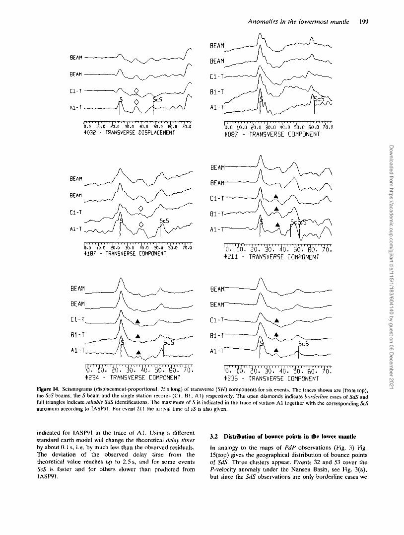
Figure 14 gives the transverse ( S H ) components for six events. The seismograms for event 32 illustrate one of the problems of single-station and network observations as opposed to array observations. A potential arrival of SdS, i.e. a reflection of S at a lower mantle discontinuity, is indicated by an open diamond. A strong onset can be identified in trace A l , but this phase is almost completely absent a t C1, although the Fresnel zones at the corresponding bounce points overlap almost completely. Due to this strong variation of the energy from A1 to C1, SdS has to be classified as a borderline case for event 32 and serves as a warning that care should be taken, when such phases are correlated, especially across large distances. The same argument holds also for event 187, whereas the seismograms of event 87 are not indicative for a phase produced in the lower mantle. Reliable identifications of SdS (full triangles), i.e. observation of a phase that is consistent across the array and occurs between S and ScS with a slowness between that of S and ScS, are given for events 211, 234 and 236. That it is possible to increase the quality of the ScS phase by beam forming can be seen for event 87, 187 and 234.

To show that the arrival time of ScS with respect to the S arrival time is also affected by the anomalies in the lower mantle, the delay time between these two phases is

Dow



ecember 2021


BE A f l -----A B E A M

r b.0 20.0 Jo.0 da.0 do.0 40.0 do.0 90.0 to32 - TRANSVERSE DISPLACEMENT

A 1 - T

mt , 1 1 1

b.0 20.0 210.0 A.0 do.0 56.0 40.0 7G t187 - TRANSVERSE COMPONENT

Bl-T>

A l - T a

'0. i 0 . 70. 30. 40. so. 20. f o . I I , , , , ' I , I , , , I 0 I , , , , I , I T

#234 - T R A N S V E R S E C O M P O N E N T

B E A M O E A M B

A 1 - T

'0.0 JO.0 20.0 40.0 40.0 40.0 60.0 90.0 I , , , , I , ( I , , , ! " ' ~ ' ' " I " ' , ' ' ' ' rT

#087 - T R A N S V E R S E C O M P O N E N T

8 1 - T

A l - T

BE A M - J L

C 1 - T \

'0. i o . 20:"%. 4o:"sQ:"EtoT , I ! I , , , I

1236 - T R A N S V E R S E C O M P O N E N T Figure 14. Seismograms (displacement-proportional, 75 s long) of transverse ( S H ) components for six events. The traces shown are (from top), the ScS beams, the S beam and the single station records (Cl, €31, A l ) respectively. The open diamonds indicate borderline cases of SdS and full triangles indicate reliable SdS identifications. The maximum of S is indicated in the trace of station A1 together with the corresponding ScS maximum according to IASP91. For event 211 the arrival time of sS is also given.

indicated for IASP91 in the trace of Al . Using a different standard earth model will change the theoretical delay times

3.2 Distribution of bounce points in the lower mantle

by about 0.1 s, i.e. by much less than the observed residuals. In analogy to the maps of PdP observations (Fig. 3) Fig. The deviation of the observed delay time from the 15(top) gives the geographical distribution of bounce points theoretical value reaches up to 2.5s, and for some events of SdS. Three clusters appear. Events 32 and 53 cover the ScS is faster and for others slower than predicted from P-velocity anomaly under the Nansen Basin, see Fig. 3(a), IASP91. but since the SdS observations are only borderline cases we

Dow



ecember 2021

200 M . Weber


SdS gp

9

J

scs x NP

+'1

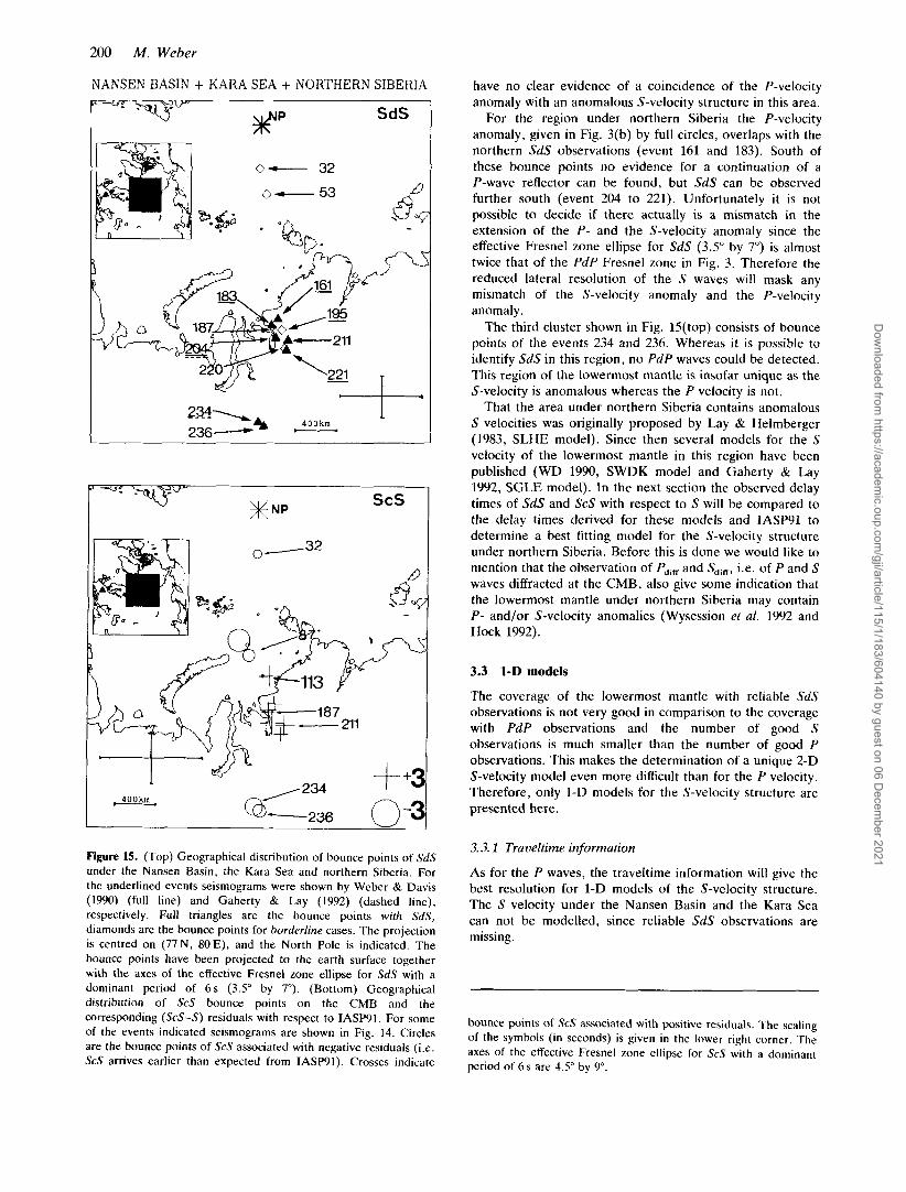
Figure 15. (Top) Geographical distribution of bounce points of SdS under the Nansen Basin, the Kara Sea and northern Siberia. For the underlined events seismograms were shown by Weber & Davis (1990) (full line) and Gaherty & Lay (1992) (dashed line), respectively. Full triangles are the bounce points with SdS, diamonds are the bounce points for borderline cases. The projection is centred on (77 N, 80 E), and the North Pole is indicated. The bounce points have been projected to the earth surface together with the axes of the effective Fresnel zone ellipse for SdS with a dominant period of 6 s (3.5" by 7"). (Bottom) Geographical distribution of ScS bounce points on the CMB and the corresponding (ScS-S) residuals with respect to IASP91. For some of the events indicated seismograms are shown in Fig. 14. Circles are the bounce points of ScS associated with negative residuals (i.e. ScS arrives earlier than expected from IASP91). Crosses indicate

have no clear evidence of a coincidence of the P-velocity anomaly with an anomalous S-velocity structure in this area.

For the region under northern Siberia the P-velocity anomaly, given in Fig. 3(b) by full circles, overlaps with the northern SdS observations (event 161 and 183). South of these bounce points no evidence for a continuation of a P-wave reflector can be found, but SdS can be observed further south (event 204 to 221). Unfortunately it is not possible to decide if there actually is a mismatch in the extension of the P - and the S-velocity anomaly since the effective Fresnel zone ellipse for SdS (3.5" by 7") is almost twice that of the PdP Fresnel zone in Fig. 3 . Therefore the reduced lateral resolution of the S waves will mask any mismatch of the S-velocity anomaly and the P-velocity anomaly.

The third cluster shown in Fig. 15(top) consists of bounce points of the events 234 and 236. Whereas it is possible to identify SdS in this region, no PdP waves could be detected. This region of the lowermost mantle is insofar unique as the S-velocity is anomalous whereas the P velocity is not.

That the area under northern Siberia contains anomalous S velocities was originally proposed by Lay & Helmberger (1983, SLHE model). Since then several models for the S velocity of the lowermost mantle in this region have been published (WD 1990, SWDK model and Gaherty & Lay 1992, SGLE model). In the next section the observed delay times of SdS and ScS with respect to S will be compared to the delay times derived for these models and IASP91 to determine a best fitting model for the S-velocity structure under northern Siberia. Before this is done we would like to mention that the observation of P,,, and Sdi,, i.e. of P and S waves diffracted at the CMB, also give some indication that the lowermost mantle under northern Siberia may contain P- and/or S-velocity anomalies (Wysession et al. 1992 and Hock 1992).

3.3 1-D models

The coverage of the lowermost mantle with reliable SdS observations is not very good in comparison to the coverage with PdP observations and the number of good S observations is much smaller than the number of good P observations. This makes the determination of a unique 2-D S-velocity model even more difficult than for the P velocity. Therefore, only 1-D models for the S-velocity structure are presented here.

3.3.1 Traveltime information

As for the P waves, the traveltime information will give the best resolution for 1-D models of the S-velocity structure. The S velocity under the Nansen Basin and the Kara Sea can not be modelled, since reliable SdS observations are missing.

bounce points of ScS associated with positive residuals. The scaling of the symbols (in seconds) is given in the lower right corner. The axes of the effective Fresnel zone ellipse for ScS with a dominant period of 6 s are 4.5" by 9".

Dow



ecember 2021


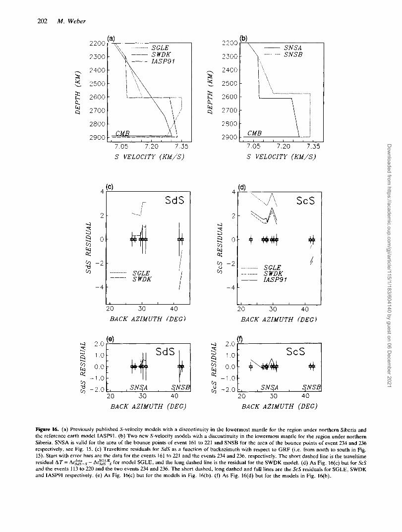
The S velocity for IASP91 and two previously published models with a discontinuity in the lowermost mantle is given in Fig. 16(a). Whereas SWDK is able to fit the SdS delay times for the northern cluster it fails for the southern cluster, as shown in Fig. 16(c). SGLE deviates on average by +2.5 s in the northern and about -2 s in the southern cluster, see also Gaherty & Lay (1992) for similar misfits. Two different velocity models for the two clusters will be needed to explain the data. This is also justified by the fact that the two clusters are more than 500 km apart in the lower mantle in Fig. 15(top), which shows that the Fresnel zones of the SdS waves for the two clusters are well separated, whereas the effective Fresnel zones in Gaherty & Lay (1992) are about twice this size since they use long-period data. SWDK will be a good starting model for the northern cluster, whereas more severe modifications for the southern cluster will be necessary.

The ScS phase will be helpful in getting an idea of the S velocity in the D" layer. Fig. 16(d) gives the ScS residual for SGLE, SWDK and IASP91. As already noted in W D , SWDK, which was derived by assuming the same reflector depth and a velocity contrast of 3 per cent as in PWDK, has a residual of about 1 to 2 s for ScS for the northern cluster and this misfit can be eliminated if the S-velocity jump is reduced to about 2 per cent. Since for all three models the residual for ScS is negative for the events 234 and 236, but positive for the northern cluster, different models for the two regions will be needed.

To demonstrate the pattern of the ScS residuals, the geographical distribution of ScS bounce points on the CMB with the corresponding residuals with respect to IASP91 is given in Fig. 15(bottom). A similar pattern of negative-to- positive-to-negative residuals is visible in Gaherty & Lay (1992) for residuals between SdS/SDS and ScS. Due to the fact that the picking of the SdS-wave group, and especially of SdS versus SDS, is somewhat ambiguous (see Fig. 14 and error bars in Fig. 16) only the more reliable residual between S and ScS is shown.

A shift in the actual location of the event will result in a change of the traveltime difference between ScS and S. It has been shown (e.g. Engdahl & Gubbins 1987 and Kennett & Engdahl 1991) that these mislocation can reach up to 0.4" for events in the Aleutians, i.e. for event 32. This increase in distance decreases the delay time at^^^^^ by about 1 s. Therefore, the ScS residual of -0.9s for event 32 can be explained completely by this effect. Fortunately, the mislocation vectors for the other events shown in Fig. 15 are smaller, i.e. about 0.1" (see e.g. Kennett & Engdahl 1991) and the positive residuals will become about 0.2 s larger and the negative residuals will decrease by the same amount, i.e. this change is small for all non-Aleutian events. The mislocation can also not explain the rapid change from negative residuals [event 87 in Fig. 15(bottom)] to positive residuals [event 113 in Fig. lS(bottom)]. Since the distance of the bounce points of event 87 to the first P c P bounce point with positive residual (event 113) is only 160 km, i.e. of the order of the small axis of the ScS Fresnel zone (Fig. lS(bottom)], strong lateral variations must be present in this region of the lower mantle, and probably therefore n o reliable SdS can be detected in this transition region.

An increase of the delay between S and ScS by about 1 s can be achieved by a shorter traveltime for S or an increased

traveltime for ScS, i.e. either by an S-velocity increase in the mid-mantle of about 0.5 per cent, an S-velocity reduction in D" by 1 per cent or an increase of the depth of the CMB by about 10 km. The best way to get some control over the models is therefore by using SdS together with ScS.

Figure 16(b) gives the models for the northern and the southern cluster of SdS observations in Fig.15 (top), i.e. SNSA and SNSB, respectively. The residuals for SdS and ScS for the two models are given in Figs 16(e) and (f) respectively. These models give a good fit to the data and are therefore adequate representations of the lower mantle in these regions. It becomes also obvious that two models, SNSA with hr,,=2610km and A ~ , ~ = 2 . 3 per cent and SNSB with hreE = 2575 km and Au.* = 2.6 per cent, can give a much better fit to the observations than a single model like SGLE. The amount and the quality of the data is not good enough to eliminate trade-offs, especially since the error bars for SdS will accomodate a variation of f15 km of hrcR and the error bars in ScS allow a variation of f 0 . 1 per cent of us in D". Therefore, these two models are only representatives of a class of possible models able to explain the SdS and ScS traveltimes.

3.3.2 Amplitude information

The effect of the thickness D of a transition zone and the S-velocity contrast Au5 at a discontinuity in the lower mantle on the amplitudes of the SdS wave group is shown in Fig. 17. To be able to compare the results for the S-wave modelling with the results of the P-wave modelling, the SWDK model is used as the reference here; it has a reflector in the same depth and also a 3 per cent velocity contrast, like PWDK. Choosing the dominant period of the S wave at 4 s gives a wavelength I of the S wave of 29 km, i.e. a wavelength almost identical to the wavelength of the P wave in Fig. 8 (27 km).

One of the main differences between the P and the S H seismograms (Figs 8 and 17 respectively) is that the core reflection ScS (see Fig. 17e for the phase identification) is a very strong arrival in comparison to PcP. Similar to the PdP-wave group, the SdS-wave group, i.e. SdS and SDS, decreases significantly in amplitude if the first-order discontinuity in SWDK is replaced by a transition zone, see Fig. 17(d), whereas the ScS phase is almost unaffected.

To understand the systematic variation of the amplitude ratio of the SdS-wave group for the four models from Figs 17(a) and (b) with respect to the SdS wave group for SWDK, Fig. 17(f) shows this ratio as a function of distance. The reduction in the amplitudes is very similar t o the reduction observed for the P waves, see Fig. 8(f), since introducing a transition zone affects the amplitude ratios for shorter distances more severely than for larger distances. A reduction of the velocity contrast (Fig. 17b) lowers the amplitudes of the SdS-wave group for the new models with respect to SWDK roughly proportional to the ratio of the velocity contrasts between the two models, i.e. to about 1/3 if the velocity contrast ratio is 1/3.

The problem of inadequate signal-to-noise conditions is even more severe for the S waves than for the P waves. This limits the resolution attainable with the amplitude information for SdS t o about *2 per cent in the velocity contrast and for the thickness D of a transition zone to

Dow



ecember 2021

202 M. Weber

2200

2300

2400

L 3 2500

2600

3 2700

2800

2900

4 2.0 1.0 2 2 0.0

2 -1.0 fx

r/, -2.0

7.05 7.20 7.35 S VELOCITY (KM/S)

:-. SdS ._ I '...(

+4 1 ............ I SGLE

S WDK I I

I 1 I I I

20 30 40

BACK AZIMUTH f D E G )

20 30 40 BACK AZIMUTH ( D E G )

2800 1 \ i CMB

7.05 7.20 7.35 ........ 2900

I I 1 I I I I

S VELOCITY (KM/S)

............ SGLE S W D K IASPS I

_ _ _ _ _ _

L I I I I 4

20 30 40

BACK AZIMUTH f D E G )

, S N S A , SNSA 20 30 40

BACK AZIMUTH ( D E G )

Figure 16. (a) Previously published S-velocity models with a discontinuity in the lowermost mantle for the region under northern Siberia and the reference earth model IASP91. (b) Two new S-velocity models with a discontinuity in the lowermost mantle for the region under northern Siberia. SNSA is valid for the area of the bounce points of event 161 to 221 and SNSB for the area of the bounce points of event 234 and 236 respectively, see Fig. 15. (c) Traveltime residuals for SdS as a function of backazimuth with respect to GRF (i.e. from north to south in Fig. 15). Stars with error bars are the data for the events 161 to 221 and the events 234 and 236, respectively. The short dashed line is the traveltime residual AT = At%$-.$ - At:Zk-Es for model SGLE, and the long dashed line is the residual for the SWDK model. (d) As Fig. 16(c) but for ScS and the events 113 to 220 and the two events 234 and 236. The short dashed, long dashed and full lines are the ScS residuals for SGLE, SWDK and IASP91 respectively. (e) As Fig. 16(c) but for the models in Fig. 16(b). (f) As Fig. 16(d) but for the models in Fig. 16(b).

Dow



ecember 2021


2300 2200 r Y - 7 2400 T

5 2 7 0 0 - 4 - 2800

2900t,,,,;-T', J 7.00 7.20 7.40

S VELOCITY (KM/S)

65' 75' A05'

65' 7 5 O

.O S VELOCITY (KM/S)

65' 75'

s 1.0 2 0.8

2 0.6 4 3 0.4

Cfl 0.2 U (K

0

- 4

....__.--

1 , I I I I I I

6a 72 76 ao DISTANCE (UEG)

Figure 17. The effect of the thickness D of a transition zone and the S velocity contrast A U , ~ in the lower mantle on the amplitudes of the SdS wave group. The dominant period of the S wave is 4 s and the wavelength A is 29 km. (a) S velocity of model SWDK (hreR = 2605 km, A U , ~ = 3.0 per cent) and of two models with transition zone thickness D equal to 2 and 4A. (b) SWDK and two models with A U . ~ = 1 per cent and 2 per cent at the discontinuity, respectively. (c) Seismogram section (displacement) of the transversal (SH) components for SWDK and a source in 131 km depth. The seismograms are computed with the reflectivity method. The reduction slowness is 9.3 s/= (d) As Fig. 17(c) but for the model with D = 4A. (e) Traveltimes of S, SDS, SdS and ScS. Distance-time frame and reduction velocity as in Fig. 17(c). (f) Amplitude ratio of the SdS-wave group for the four models from Figs 17(a) and (b) with respect to the SdS wave group for SWDK (full triangle) as a function of distance.

Dow



ecember 2021

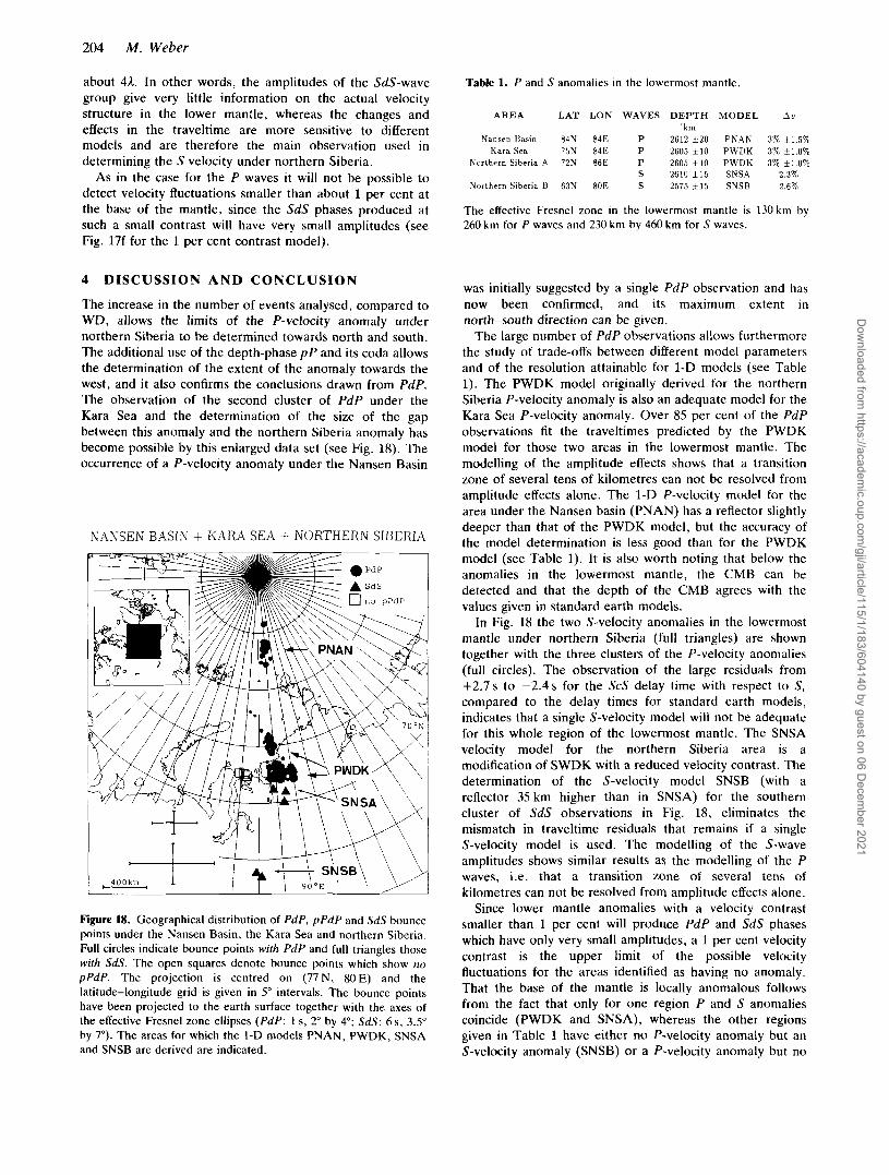
204 M. Weber

about 4A. In other words, the amplitudes of the SdS-wave group give very little information on the actual velocity structure in the lower mantle, whereas the changes and effects in the traveltime are more sensitive to different models and are therefore the main observation used in determining the S velocity under northern Siberia.

As in the case for the P waves it will not be possible t o detect velocity fluctuations smaller than about 1 per cent a t the base of the mantle, since the SdS phases produced at such a small contrast will have very small amplitudes (see Fig. 17f for the 1 per cent contrast model).

4 DISCUSSION A N D CONCLUSION

The increase in the number of events analysed, compared to WD, allows the limits of the P-velocity anomaly under northern Siberia to be determined towards north and south. The additional use of the depth-phase pP and its coda allows the determination of the extent of the anomaly towards the west, and it also confirms the conclusions drawn from PdP. The observation of the second cluster of PdP under the Kara Sea and the determination of the size of the gap between this anomaly and the northern Siberia anomaly has become possible by this enlarged data set (see Fig. 18). The occurrence of a P-velocity anomaly under the Nansen Basin


Figure 18. Geographical distribution of PdP, p P d P and SdS bounce points under the Nansen Basin, the Kara Sea and northern Siberia. Full circles indicate bounce points with PdP and full triangles those with SdS. The open squares denote bounce points which show no p P d P . The projection is centred on (77N, 80E) and the latitude-longitude grid is given in 5" intervals. The bounce points have been projected to the earth surface together with the axes of the effective Fresnel zone ellipses ( P d P : 1 s, 2" by 4"; SdS: 6 s, 3.5" by 7"). The areas for which the I-D models PNAN, PWDK, SNSA and SNSB are derived are indicated.

Table 1. P and S anomalies in the lowermost mantle.

AREA LAT LON WAVES D E P T H MODEL A v

Nansen Basin 84N 84E P 2612 120 P N A N 3% i l 5% Kara Sea 75N 84E P 2605 1 1 0 PWDK 3% i10%

Northern Siberia A 72N 86E P 2605 1 1 0 PWDK 3% i l 0% S 2610 *15 SNSA 2 3%

Northern Siberia B 63N 80E S 2575 1 1 5 S N S B 2 6 %

The effective Fresnel zone in the lowermost mantle IS 130 km by 260 km for P waves and 230 km by 460 km for S waves.

[km

was initially suggested by a single P d P observation and has now been confirmed, and its maximum extent in north-south direction can be given.

The large number of PdP observations allows furthermore the study of trade-offs between different model parameters and of the resolution attainable for 1-D models (see Table 1). The PWDK model originally derived for the northern Siberia P-velocity anomaly is also an adequate model for the Kara Sea P-velocity anomaly. Over 85 per cent of the PdP observations fit the traveltimes predicted by the PWDK model for those two areas in the lowermost mantle. The modelling of the amplitude effects shows that a transition zone of several tens of kilometres can not be resolved from amplitude effects alone. The 1-D P-velocity model for the area under the Nansen basin (PNAN) has a reflector slightly deeper than that of the PWDK model, but the accuracy of the model determination is less good than for the PWDK model (see Table 1). It is also worth noting that below the anomalies in the lowermost mantle, the CMB can be detected and that the depth of the CMB agrees with the values given in standard earth models.

In Fig. 18 the two S-velocity anomalies in the lowermost mantle under northern Siberia (full triangles) are shown together with the three clusters of the P-velocity anomalies (full circles). The observation of the large residuals from +2.7s to -2.4s for the ScS delay time with respect to S, compared to the delay times for standard earth models, indicates that a single S-velocity model will not be adequate for this whole region of the lowermost mantle. The SNSA velocity model for the northern Siberia area is a modification of SWDK with a reduced velocity contrast. The determination of the S-velocity model SNSB (with a reflector 35 km higher than in SNSA) for the southern cluster of SdS observations in Fig. 18, eliminates the mismatch in traveltime residuals that remains if a single S-velocity model is used. The modelling of the S-wave amplitudes shows similar results as the modelling of the P waves, i.e. that a transition zone of several tens of kilometres can not be resolved from amplitude effects alone.

Since lower mantle anomalies with a velocity contrast smaller than 1 per cent will produce PdP and SdS phases which have only very small amplitudes, a 1 per cent velocity contrast is the upper limit of the possible velocity fluctuations for the areas identified as having no anomaly. That the base of the mantle is locally anomalous follows from the fact that only for one region P and S anomalies coincide (PWDK and SNSA), whereas the other regions given in Table 1 have either n o P-velocity anomaly but an S-velocity anomaly (SNSB) or a P-velocity anomaly but no

Dow



ecember 2021


reliable or no SdS detection (Nansen Basin and Kara Sea respectively). The changes in the Poisson ratio in the different regions, assuming IASP91 if no velocity anomaly could be reliably determined, reaches values of +5.9 to -4.8 per cent with an accuracy of about f 1 . S per cent. This change in the Poisson ratio is of the same order as that determined by Wysession et al. (1992) from P,,, and S,,, phases and possibly indicates the range of the Poisson-ratio fluctuations occuring at the base of the mantle. The limitations in the resolution attainable with the data studies here are given in Fig. 18 by the elfective Fresnel zones for P and S waves in the lowermost mantle. Structures smaller than the ellipses given can not be resolved, and the actual size of the velocity anomalies in the areas of the clusters of full circles (P-velocity anomalies) and full triangles (S-velocity anomalies) may be smaller.

Since the azimuthal coverage with events in the Northwest Pacific and the G R F array is limited, we lack the proper control to determine a unique model of the lower mantle anomalies in this region. Therefore, the 2-D models presented give only the range of model parameters and allow some insight into possible trade-offs between different parameters. The most significant effect if the extension of the reflector is reduced t o realistic dimensions is that the depth of the reflector has to be up to 40 kilometres deeper than in the I-D model, if the same P-velocity contrast of 3 per cent is assumed. Another conclusion is that topography with dips of about 1.5" can be detected, but the direction of the dip (i.e. towards the source or towards the receiver) can not be resolved reliably with the data a t hand.

The main part of this paper has dealt with the anomalies under the North Pole region and northern Siberia, since only there could anomalous structures in D" be detected with the G R F array. The fact that earthquake-GRF combinations covering other areas of the lowermost mantle (see Fig. l ) , d o not show a PdP phase is, together with the limited size of the observed P - and S-velocity anomalies, an indication that the lowermost mantle will only have a limited number of areas where the velocity anomalies are strong enough to be detectable. This conclusion is in agreement with the results of Weber & Kornig (1992) who searched seismic bulletins for the anomalous phase PdP, and found that only about 3 per cent of the lowermost mantle are promising areas for strong lower mantle anomalies, whereas other areas of D" are likely to have smaller velocity fluctuations, if any.

The coverage of the anomalies given in Fig. 18 can be improved in several ways. One of them is achieved by extending the receiver array, e.g. by using the GRSN recently installed in Germany. This will give, due to its larger extension, an improved coverage of 100 to 200 km towards east and west in the lowermost mantle. The analysis of converted waves like ScP will furthermore be a valuable tool in studying the structure of the CMB (see Vidale & Benz 1992).

The conclusion that can be drawn from the joint study of P and S waves is that some areas a t the base of the mantle contain small-scale anomalies in which the P - to S-velocity ratio might vary by several per cent. We would finally like to add, that the question if this change in the velocities is due to chemical and/or thermal anomalies, can not be answered with seismological methods alone.

ACKNOWLEDGMENTS

Throughout this work I profited from several discussions with the Mathematical Geophysics group at the University of Frankfurt. I thank W. Hanka and K. Stammler for their programs to analyse and process the data. I would also like to thank D. Baumgardt, F. Kriiger, G. Miiller. J. Schlittenhardt, J. Schweitzer and Ch. Young for their comments to this paper, and the Deutsche Forschungsgemein- schaft (DFG) for financing this research. The Grafenberg- array is operated by the Bundesanstalt fur Geowissenschaf- ten und Rohstoffe (BGR) and funded by the DFG.

REFERENCES

Ahrens, T. J . & Hager, B. H., 1987. Heat transport across D", EOS Trans. Am. geophys. Un. 68, 1493.

Anderson, D. J. , 1987. Thermally induced phase changes, lateral heterogeneities in the mantle, continental roots, and deep slab anomalies, J. geophys. Res. , 92, 13968-13980.

Bataille, K. & FlattC, S. M., 1988. Inhomogeneities near the core-mantle boundary inferred from short period scattered PKP waves recorded at the GDSN, J . geophys. Res., 93, 15057- 15064.

Bataille, K., Wu, R.-S. & FlattC, S. M., 1990. Inhomogeneities near the core-mantle boundary evidenced from scattered waves: a review, Paeoph, 132, 151-173.

Baumgardt, D. R., 1989. Evidence for a P-wave velocity anomaly in D", Geophys. Res. Le t f . , 16, 657-660.

Bercovici, D., Schubert, G. & Glatzmaier, G. A,, 1989. Influence of heating mode on three-dimensional mantle convection, Geophys. Res. Lett., 16, 617-620.

Boehler, R., 1992. Melting of the Fe-FeO and Fe-FeS systems at high pressure: constraints on core temperatures, Earfh planet. Sci. Le t f . , 111, 217-227.

Boehler, R., von Bargen, N. V. & Chopelas, A,, 1990. Melting, thermal expansion, and phase transition of iron at high pressures, J. geophys. Res. , 95, 21731-21736.

Bullen, K. E., 1949. Compressibility-pressure hypothesis and the Earth's interior, Mon. Not. R. astr. SOC., Geophys. Suppl., 5,

Bullen, K. E., 1950. An earth model based on a compressibility- pressure hypothesis, Mon. Not. R . aslr. SOC., Geophys. Suppl.,

CervenL, V., Popov, M. M. & PSenEik, I., 1982. Computation of wavefields in inhomogeneous media-Gaussian beam approach, Geophys. J. R . astr. SOC., 70, 109-128.

Christensen, U. R., 1987. Formation and dynamics of a compositional boundary layer at the base of the mantle, EOS Trans. Am. geophys., Un. 68, 1488.

Christensen, U. R., 1989. Models of mantle convection: one or several layers, Phil. Trans. R . SOC. Lond . , A, 328, 417-424.

Cormier, V. F., 1985. Some problems with S, SKS and ScS observations and implications for the structure of the base of the mantle and the outer core, J. Geophys. , 57, 14-22.

Cormier, V. F., 1989. Slab diffraction of S waves, J. geophys. Res.,

Creager, K. C. & Jordan, T. H., 1986. Aspherical structure of the core-mantle boundary from P K P travel times, Geophys. Res. Le t f . , 13, 1497-1500.

Dahm, C. G., 1934. A study of dilatational wave velocity in the Earth, as a function of depth, based on a comparison of the P. P', and PcP phase, PhD thesis, Saint Louis University.

Davies, G. F. & Gurnis, M., 1986. Interaction of mantle dregs with convection: lateral heterogeneity at the core-mantle boundary, Geophys. Res. Lett., 13, 1517-1520.

355-368.

6, 50-59.

94, 3006-3024.

Dow



ecember 2021

206 M . Weber

Davies, J . H., Gudmundsson, 0. & Clayton, R. W., 1952. Spectra of mantle shear wave velocity structure, Geophys. J . lnt., 108,

Davis, J. P. & Weber, M., 1990. Lower mantle velocity inhomogeneity observed at GRF array, Geophys. Res. Lett.,

Doornbos, D. J. , 1978. On seismic wave scattering by a rough core-mantle boundary, Geophys. J . R. astr. Soc., 53, 643-662.

Doornbos, D . J. , 1988. Multiple scattering by topographic relief with application to the core-mantle boundary, Geophys. J., 92, 465-478.

Doornbos, D. J . & Vlaar, N. J. , 1973. Regions of seismic wave scattering in the Earth’s mantle and precursors to P K P , Nature, 243, 58-61.

Doornbos, D. J. & Hilton, T., 1989. Models of the core-mantle boundary and the travel times of internally reflected core phases, J. geophys. Res., 94, 15741-15751.

Doornbos, D. J., Spiliopoulos, S. & Stacey, F. D., 1986. Seismological properties of D” and the structure of a thermal boundary layer, Phys. Earth planet. Inter., 41, 225-239.

Dziewonski, A,, 1984. Mapping the lower mantle: determination of lateral homogeneity in P velocity up to degree and order 6, J . geophys. Res., 89, 5929-5952.

Dziewonski, A. & Anderson, D. L., 1984. Structure, elastic and rheological properties and density of the Earth’s interior, gravity and pressure, in Landoldt-Bornstein, Group V , Volume 2a, pp. 84-96, ed. Fuchs, K. & Soffel, H., Springer, Berlin.

Dziewonski, A. & Woodhouse, J . H., 1987. Global images of the Earth’s interior, Science, 236, 37-48.

Elsasser, W. M., Olson, P. & Marsh, B. D., 1979. The depth of mantle convection, J. geophys. Res., 84, 147-155.

Emmerich, H., 1991. A combination of finite difference methods and frequency-wavenumber filters for the modelling of the wave propagation in locally complicated media, PhD thesis, in German, University of Frankfurt.

Engdahl, E . R. 6t Gubbins, D., 1987. Simultaneous travel time inversion for earthquake location and subduction zone structure in the central Aleutian Islands, J . geophys. Res., 92, 13855-13862.

Engdahl, E. R. & Kind, R., 1986. Interpretation of broadband seismograms from central Aleutian earthquakes, Ann. Geophys., 4, B, 3, 233-240.

Fuchs, F. & Muller, G., 1971. Computation of synthetic seismograms with the reflectivity method and comparison with observations, Geophys. J . R. astr. Soc., 23, 417-433.

Gaherty, J . B. & Lay, T., 1992. Investigation of laterally heterogeneous shear velocity structure in D“ beneath Eurasia, J. geophys. Res., 97, 417-436.

Garnero, E., Helmberger. D. & Engen, G., 1988. Lateral variations near the core-mantle boundary, Geophys. Res. Letf., 15, 609-612.

Gudmundsson, 0. & Clayton, R. W., 1991. A 2-D synthetic study of global traveltime tomography, Geophys. J. Inf . , 106, 53-65.

Gudmundsson, O., Davies, J . H. & Clayton, R. W., 1990. Stochastic analysis of global traveltime data: mantle heterogeneity and random errors in the ISC data, Geophys. J. Int . , 102,

Gutenberg, B., 1914. Uber Erdbebenwellen VIIA. Beobachtungen an Registrierungen von Fernbeben in Gottingen und Folgerungen uber die Konstitution des Erdkorpers, Nachr. d . K. Ges. d . Wiss. zu Gottingen, math.-phys. Klasse, 125-177.

Haddon, R. A. W., 1982. Evidence for inhomogeneities near the core-mantle boundary, Phil. Trans. R. SOC. Lond., A, 306,

Haddon, R. A. W. & Buchbinder, G . G. R . , 1986. Wave propagation effects and the Earth’s structure in the lower mantle, Geophys. Res. Lett., 13, 1489-1492.

Haddon, R. A. W. & Buchbinder, G. G. R., 1987. S-wave

865-882.

17, 187-190.

25-43.

61-70,

scattering by 3-D heterogeneities at the base of the mantle, Geophys. Res. Lett., 14, 891-894.

Haddon, R. A. W. & Cleary, J. R., 1974. Evidence for scattering of seismic P K P waves near the core-mantle boundary, Phys. Earth planet. Inter., 8, 211-234.

Hanka, W. & Seidl, D., 1986. Signal processing of Grafenberg array data, in Ten years of the Griifenberg array, ed. Buttkus, B., Geologisches Jahrbuch, E , 35, 44-56.

Hansen, U. & Yuen, D. A, , 1988. Numerical simulations of thermal-chemical instabilities at the core-mantle boundary, Nature, 334, 237-240.

Hansen, U. & Yuen, D. A, , 1989. Dynamical influences from thermal-chemical instabilities at the core-mantle boundary, Geophys. Res. Len., 16, 629-632.

Hock, S., 1992. Determination of the ray parameter of PdlW for the study of the lowermost mantle, Diploma thesis, 1992 (in German), University of Frankfurt.

Houard, S. & Nataf, H.-C., 1992. Further evidence for the ‘Lay discontinuity’ beneath northern Siberia and the North Atlantic from short-period P waves recorded in France, Phys. Earth planet. Inter., 72, 264-275.

Houard, S. & Nataf, H.-C., 1993. Laterally varying reflector at the top of D” beneath northern Siberia, Geophys. J. Int., 115,

Inoue, H., Fukao, Y., Tanabe, K. & Ogata, Y., 1990. Whole mantle P-wave travel time tomography, Phys. Earth planet. Inter., 59, 294-328.

Jeffreys, H. & Bullen, K. E., 1940. Seismological Tables, British Association for the Advancement of Science, Burlington House, London.

Kampfmann, W. & Muller, G. , 1989. PcP amplitude calculations for a core-mantle boundary with topography, Geophys. Res. Lett., 16, 653-656.

Kennett, B. L. N. & Engdahl, E. R., 1991. Traveltimes for global earthquake location and phase identification, Geophys. J. Int.,

Knittle, E. & Jeanloz, R., 1989. Simulating the core-mantle boundary: an experimental study of high-pressure reactions between silicates and liquid iron, Geophys. Res. Lett., 16,

Knittle, E. & Jeanloz, R., 1991. The high pressure phase diagram of Fe,,O: a possible constituent of the Earth’s core, J. geophys. Res., %, 16169-16180.

Kruger, F. & Weber, M., 1992. The effect of low velocity sediments on the mislocation vectors of the GRF array, Geophys. J. Int.,

Lavely, E. M., Forsyth, D. W. & Friedemann, P., 1986. Scales of heterogeneity near the core-mantle boundary, Geophys. Res. Lett., W, 1505-1508.

Lay, T., 1989. Structure of the core-mantle transition zone: a chemical and thermal boundary layer, EOS Trans. Am. geophys. Un. , 70, 49.

Lay, T. & Helmberger, D. V., 1983. A lower mantle S-wave triplication and the shear velocity structure of D”, Geophys. J . R. astr. SOC., 75, 799-837.

Loper, D. E. & McCartney, K., 1986. Mantle plumes and the periodicity of magnetic field reversals, Geophys. Res. Lett., 13,

Loper, D. E . & Stacey, F. D., 1983. The dynamical and thermal structure of deep mantle plumes, Phys. Earth planet. Inter., 33,

Menke, W., 1986a. Effect of heterogeneities in D“ on the decay rate of PdiR. J. geophys. Res., 91, 1927-1933.

Menke, W., 1986b. Few 2-50 km corrugations on the core-mantle boundary, Geophys. Res. Lett., 13, 1501-1504.

Muller, G., 1977. Earth-flattening approximation for body waves derived from geometric ray theory-improvements, corrections and range of applicability, J. Geophys., 42, 429-436.

168- 182.

105,429-465.

609-612.

108,387-393.

1525-1528.

304-317.

Dow



ecember 2021


Miiller, G. , 1985. The reflectivity method: a tutorial, J. Geophys.,

Neuberg, J. & Wahr, J. , 1991. Detailed investigation of a spot on the core-mantle boundary using digital PcP data, Phys. Earth planet. Inter., 68, 132-143.

Olson, P., Schubert, G. , Anderson, S. & Goldman, P., 1987. Boundary layer dynamics and small scale structure at the base of the mantle, EOS Trans. Am. geophys. Un. , 68, 1488.

Popov, M. M., 1982. A new method of computation of wave-fields using Gaussian beams, Wave Motion, 4, 85-95.

Pullian, R. J. & Johnson, L. R., 1992. What patterns of heterogeneity in the Earth's mantle can be revealed by seismic travel time tomography?, Phys. Earth planet. Infer., 73,

Ross, M., Young, D. A. & Grover, R., 1990. Theory of the iron phase diagram at Earth core conditions, 1. geophys. Rex , 95,

Ruff, L. J . & Lettvin, E., 1984. Short period P-wave amplitudes and variability of the core shadow zone boundary, EOS Tram. Am. geophys. Un., 65, 999.

Schenk, T., Miiller, G. & Briistle, W., 1989. Long-period precursors to pP from deep-focus earthquakes: the Moho underside reflection p M P , Geophys. J. Int., 98, 317-327.

Schlittenhardt, J., 1986. Investigation of the velocity and Q structure of the lowermost mantle using P c P / P amplitude ratios from arrays at distances of 70"-84", J. Geophys., 60, 1-18.

Schlittenhardt, J . , Schweitzer, J . & Miiller, G., 1985. Evidence against a discontinuity at the top of D", Geophys. J. R. astr.

Schubert, F., Olson, P., Anderson, C. A. & Goldman, P., 1987. Mantel plumes, solitons and the D" layer, EOS Trans. Am. geophys. Un. , 68, 1488.

Schweitzer, J., 1990. Study of the velocity structure in the lower mantle and in the core-mantle boundary region below the Pacific with S waves, PhD thesis (in German), University of Frankfurt.

Silver, P. G., Carlson, R. & Olson, P., 1988. Deep slabs, geochemical heterogeneity and the large-scale structure of mantle convection: investigation of an enduring paradox, Ann. Rev. Earth planet. Sci., 16, 477-541.

Sleep, N. H., 1988. Gradual entrainment of a chemical layer at the base of the mantle by overlying convection, Geophys. J. R. ustr. Soc., 95, 437-447.

Spies, T., 1991. Study of the structure in the region of the boundary of the inner core with PKP phases, PhD thesis (in German), University of Frankfurt.

Stacey, F. D. & Loper, D. E., 1983. The thermal boundary layer interpretation of D" and its role as a plume source, Phys. Earth planet. Inter., 33, 45-55.

Stixrude, L. & Bukowinski, M. S. T., 1992. Stability of (Mg, Fe)SiO, perovskite and the structure of the lowermost mantle, Geophys. Res. Lett., 19, 1057-1060.

Tanimoto, T., 1987. The three-dimensional shear wave structure in the mantle by overtone waveform inversion-I. Radial seismogram inversion, Geophys. J. R. astr. SOC., 89, 713-740.

Tanimoto, T., 1990. Long wavelength S-velocity structure throughout the mantle, Geophys. J. lnt., 100, 327-336.

Vidale, J . E. , 1987. Waveform effects of a high-velocity, subducted slab, Geophys. Res. Lett., 14, 542-545.

Vidale, J . E. & Benz, H. , 1992. A sharp and flat section of the core-mantle boundary, Nature, 359, 627-629.

Vidale, J . E. & Benz, H . , 1993. Mapping fine structure near the base of the mantle, Nature, 361, 529-532.

58, 153-174.

109-151.

21713-21716.

SOC., 81, 295-306.

Vidale, J. E., Williams, 0. & Houston, H., 1991. Waveform effects of a metastable olivine tongue in subducting slabs, Geophys. Res. Lett., 18, 2201-2204.

Vinnik, L. P., Lukk, A. A. & Nikolaev, A. V., 1972. Inhomogeneities in the lower mantle, Phys. Earth planet. Inter., 5, 328-331.

Weber, M., 1988. Computation of body-wave seismograms in absorbing 2-D media using the Gaussian beam method: comparison with exact methods, Geophys. J., 92, 9-24.

Weber, M., 1990. Subduction zones-their influence on traveltimes and amplitudes of P-waves, Geophys. J. Int., 101, 529-544.

Weber, M. & Davis, J . P., 1990. Evidence of a laterally variable lower mantle structure from P and S waves, Geophys. 1. Int.,

Weber, M. & Kornig, M., 1990. Lower mantle inhomogeneities inferred from PcP precursors, Geophys. Res. Lett., 17,

Weber, M. & Kornig, M., 1992. A search for anomalies in the lowermost mantle using seismic bulletins, Phys. Earth planet. Inter., 73, 1-28.

Wiens, D. A., 1987. Effects of near source bathymetry on teleseismic P waveforms, Geophys. Res. Lett., 14, 761-764.

Wright, C., 1973. Array studies of P phases and the structure of the D" region of the mantle, J . geophys. Res., 78,4965-4982.

Wright, C. & Cleary, J. R., 1972. P wave travel-time gradient measurements for the Warramunga seismic array and lower mantle structure, Phys. Earth planet. Inter., 5, 213-230.

Wright, C. & Lyons, J . A,, 1980. Further evidence for radial velocity anomalies in the lower mantle, Pageoph, 119,

Wright, C., Muirhead, K. J. & Dixon, A. E., 1985. The P wave velocity structure near the base of the mantle, J. geophys. Res.,

Wysession, M. E . & Okal, E . A., 1989. Regional analysis of D" velocities from the ray parameters of diffracted P profiles, Geophys. Res. Lett., 16, 1417-1420.

Wysession, M. E., Okal, E. A. & Bina, C. R., 1992. The structure of the core mantle boundary from diffracted waves, J . geophys. Res., 97, 8749-8764.

Wysession, M. E., Okal, E. A. & Miller, K. L., 1991. Intraplate seismicity of the Pacific Basin, Pageoph., 135, 1913-1988.

Young, C. J. & Lay, T., 1987. Evidence for a shear velocity discontinuity in the lower mantle beneath India and the Indian Ocean, Phys. Earth planet. Inter., 49, 37-54.

Young, C. J. & Lay, T., 1989. The core shadow zone boundary and lateral variations of the P velocity structure of the lowermost mantle, Phys. Earrh planet. Inter., 54, 64-81.

Young, C. J. & Lay, T., 1990. Multiple phase analysis of the shear velocity structure in the D" region beneath Alaska, J. geophys. Res., 95, 17386-17402.

Yuen, D. A. & Peltier, W. R., 1980. Mantle plumes and the thermal stability of the D" layer, Geophys. Res. Lett., 7,

Zhang, S. & Yuen, D. A., 1987. Deformation of the core-mantle boundary induced by spherical shell, compressible convection, Geophys. Res. Lett., 14, 899-902.

Zhang, S. & Yuen, D. A., 1988. Dynamical effects on the core-mantle boundary from depth-dependent thermodynami- cal properties of the lower mantle, Geophys. Res. Lett., 15,

Zhou, H.-W., 1990. Observation of earthquake stress axes and seismic morphology of deep slabs, Geophys. J. lnt., 103,

102, 231-255.

1993- 1996.

137- 162.

90, 623-634.

625-628.

451-454.

377-401,

Dow



ecember 2021

AP

PE

ND

IX:

EV

EN

TS

# 1 2 3 4 5 6 7 8 9 10

11

12

I3

14

15

16

17

18

19

20

21

22

23

24

25

26

27

28

29

30

31

32

33

34

35

36

37

38

39

40

41

42

43

44

45

46

pz

48

49

50

51

DA

TE

83 6

28

87 1

1 17

85 12 30

87 4 I8

8038

88 1

1 30

90

7 25

88 4 I9

89 3 17

83 2 14

87 621

90 5 21

89 5 19

88 12 22

90 2 27

88 12 11

88 924

87 8 14

90 1

10

84 123

90 121

86 1

0 26

88 6 3

89 9 15

88 123

89

6 14

88 5 25

87 7 6

84 10 25

89 9 9

82 6

4

87 3 21

89 12

1 90

9 29

80 1

19

85 3 23

89 1

1 24

89 1

1 12

89

10 7

87 2 1

8 87

56

87 3 6

83 4 3

90 9

18

85 5 9

85 1

1 16

79 10

18

88 3 8

81 2

4

81 2 1

90

9 27

TIM

E

3: 25:17.1

9: 38:12.3

12: 41: 2.7

2: 1:38.9

9: 47:45.3

8: 55:30.6

14: 42:42.1

22: 5: 4.3

17: 26:21.3

8: 1

0: 3.6

5: 46:IO.O

13: 0: 9.8

2: 21:56.4

10: 42:12.6

21: 49:56.1

5: 18:23.4

8: 10:45.6

17: 39:32.2

13: 10:12.3

22: 6: 6.6

1: 59:40.1

4: 43:27.5

15: 39:23.0

9: 48: 9.2

2: 45z35.7

0: 35.58.3

14: 5:17 7

0: 23:25.6

12. 37:15.5

10: 38: 6.

8 3: 1: 4.1

10: 41:36.0

5. 6:lZ.l

16: 11:27.5

7: 2:

35.0

21, 35:13.0

12: 49: 6.4

0: 0:21.7

17: 42:36.3

0: 0

:52.

5 4: 18:24.7

13: 48:41.5

19: 14: 5.1

3: 18:39.5

19

5:21

.6

0: 23:50.9

3: 35.

26.9

16: 27:18.9

5. 13:19 0

13. 17:11.3

21 7:38.7

62

5.6

68.6

68

5.8

68.8

350 8

67

5.9

71.8

351.6

144

5.6

69.0

351.7

49

5.7

76.9

352.9

149

5.0

72.0

353.0

33

6.1

75.9

354.4

34

6.3

76 8

356.4

33

5.6

77.4

356.9

104

6.2

76.7

358.2

77

5.5

77 1

358.6

33

5.4

78.9

359.0

55

5.0

77.7

359.0

33

5.3

79.3 359.6

118

5.8

77.7

0.3

33

5.7

78.9

0.5

103

5.4

77.8

0.6

33

5.3

79.1

0.9

214

5.5

77.4

0.9

165

5.2

78.0

1.1

33

5.5

79.4

3.1

48

5.6

79.6

3.6

33

5.4

79.4

3 7

40

5.8

80.5

3.9

33

5.9

79.5

3 9

56

5.4

79.3

4.2

33

5.4

79.6

4.7

59

5.9

79.3

5.5

93

6.1

78.8

5.6

43

5.7

79.2

6.0

33

5.3

79.4

6.2

77

5.3

74.2

353.0

-

LA

T

60.2

2 58.61

61.5

4 61.37

58.39

61.35

53.66

56 45

58.64

54.97

54.21

53.58

54.31

54.0

5 52.01

53.38

51.87

53.42

52.12

53.29

51.98

53.76

53.11

51 63

51.4

0 51.55

50.55

51.51

51.6

8 51.27

51.6

0 52.06

51.6

5 51.36

51.32

52.62

51.32

51.2

5 51

.12

51.30

51.07

51.14

51 98

51.43

51 47

51.58

51.8

6 51 34

51.34

51.34

51.69

__

__

- - ~ - - ~ - - ~ - - ? ~ ~ - - - - - - - ~ - ~ - - ? ? ? ?

LO

N

-141.29

-143

.10

-160.34

-150.66

-152.96

-152.27

-156.75

-156.38

-155.75

-159.24

-162

.60

-163.49

-165

.57

-166.24

-166.90

-166.89

-167.97

-169.11

-169.24

-169.64

-170.01

-170

.05

-170.38

-173

.33

-174.27

-174.32

-174.57

-174

72

-175.21

-175.81

-177.33

-177.55

-178.07

-178.26

-178

49

-178.87

-178

93

-178.91

-179.21

-179.30

-179.84

179.59

179.26

177.98

177 91

177.26

177.13

176 86

176.62

176 78

176.31

h m

b A

19

6.1

68.7

BA

Z

PdP 1

PcP

1 pPdP

SdS

345.8

I -

I I

I 346.2

- 350.8

1 - 1

I 1

I

I7

~?

8.6

l7

.-

4L i2

53

54

55

56

57

58

59

60

61

62

63

64

65

66

67

68

69

70

71

72

73

74

75

76

77

78

79

80

81

82

83

84

85

86

87

88

89

90

91

92

93

94

95

96

97

98

99

I01

I oa

DA

TE

83 1

24

82 7 31

85 10 30

88 2 16

88 2 16

88 2 16

79 9 23

87 8 22

88 5 1

8 85 7 31

88 2 7

88 2 13

89 6 20

85 9 10

89 5 25

89 10 9

85 8 1

1 86 1

1

87 7 1

1 89 127

85

3 6

80 3 22

89 8 30

86 4 1

85 5 25

85 5 19

86 6 17

89 7 18

83 4 15

87 1

0 6

87 106

89 9 15

83 4 4

84 6 1

87

4 1

6 83 7 24

90 8 14

82 1

1 14

87 7 6

78 12

1 82 9 26

88 7 25

86 3 2

85 8 24

87 7 1

1 87 5 12

87 9 8

88 3 14

81 2

26

87 9 19

88 12 22

~- O

BSE

RVE

D:

+ =Y

ES

, - =

NO

, ?

= B

OR

DER

LIN

E C

ASE

TIM

E

13 2372

6 29155

19 5375

4 22362

5 44 38 7

3 29

44 4

10 17208

5 9144

6 13464

7 37547

I8 15 56

23 56 58 8

18 7436

126 4

4

20 13 334

18 187

9 59 44 2

22 10 270

14 52276

8 34513

22 31 53 3

10 27 40

1 11

38 128

13 40 45 2

23 29 21 7

8 7482

0 42

35 4

10 41 14 6

14 51 59

1 20 18 34 8

20

11 35

1 18 34 13 2

19 4 206

5 54518

110206

23 73

1 0

15 59 7 9

8 29 20 3

23 22 6 2

I1 4

3 28 3

19285

23 42 35 2

3 14

41 8

16 0

34

5 13 152

4

3590

13 35 16 2

19 17 4

I 14 39 31 8

21 58

08

144135 ~

LA

T

51.38

51.76

51.80

51.56

51.50

51.56

52.29

52.16

52.11

52.40

50.79

50.64

52 53

60.39

51.68

51.75

54.14

56.04

55.14

56.23

55 24

55.7

1 55.61

54.65

54 06

53.61

53 88

53 38

53.39

53 00

52.96

53.26

52.93

53.70

54.96

53.93

53 1

1 52.99

53.43

50 93

50.05

50.95

51 68

50.20

50 20

49.99

49 61

49.67

49 81

49.65

49 57

~ __

__

L

ON

176.25

176.14

175.53

175.04

175.05

174.97

174.03

174.07

174

18

173.49

173.47

173.41

172.51

168.81

172.13

171.90

168.73

165

01

165.50

164.40

162.04

161.48

161.36

161.58

160 99

160.53

160 39

160.38

160.31

159 87

159.97

159 77

159.86

159.32

157.99

158.37

158.64

158 67

158.32

158.86

158.80

157.70

156.94

156 72

156 28

156 28

156 36

156 31

156 25

156 32

156.

22

__

__

h m

b A

B

AZ

33

55 789

97

38

63 785

97

33

5 7

78 4

10 0

33

6 0

78 6

10 3

33

56 787

103

33

53 786

104

43

5 8

77 8

10 8

33

5 6

77 9

10 8

33

5 3

78 0

10 8

46

58 776

11 1

33

63 792

11 5

33

52 793

11 5

33

53 773

11 7

17

58 692

118

33

54 78

1 12

1 33

61 780

123

50

6 0

75 2

13 6

27

52 72

8 15

1 33

54 737

151

28

5 5

72 5

15 4

47

59 730

171

69

5 7

72 5

17 2

73

5 9

72 5

17 4

35

58 735

175

46

60 739

181

63

6 2

74 2

18 5

33

60 740

185

33

55 744

187

65

5 9

74 4

I8 7

33

5 3

74 7

19 1

34

6 2

74 7

19 1

52

57 744

192

38

6 1

74 7

19 2

98

5 3

73 9

19 2

310

51 724

195

180

62 735

196

33

5 1

74 2

199

92

5 8

74 4

19 8

149

54 739

199

42

5 5

16 4

20 5

44

5 6

77 2

20 9

85

57 76 1

21 2

118

57 752

214

80

5 2

76 5

22 2

75

5 5

76 5

22 4

47

54 76

6 22

4 83

5 7

770

225

61

54 769

22 5

33

5 6

76 4

22 5

85

5 5

77 0

22 5

33

54 770

226

?dP -

+ + + ? + ? + + + 7 + ? + + + ? ? ? ? ? ? + ? ? + ? 7 ? t t i

+ i + i _

.

Dow



ecember 2021

-

# -

103

104

105

106

107

108

109

110

111

112

113

114

115

116

117

118

119

120

121

122

123

124

125

126

127

128

129

130

131

132

133

134

135

136

137

138

139

140

141

142

143

144

145

146

147

148

149

Isa

151

152 153

DA

TE

88

8 1

4 87

9 6

78

10

28

82 1

0 17

88

10

24

89 1

1 10

87

9 6

89

I1

10

84 7

23

88 1

0 23

88

10

22

85 9 I

8 84

11

2

83 5

29

84 3

21

90 1

24

82 5

24

80 6

24

78 9

3

81 1

1 26

86

3 2

8 84

10

20

87 9

26

84 1

1 17

84

8 2

2 86

2 1

9 85

2 8

88

19

87

7 1

5 86

2 1

4 89

5 1

7 89

10

4

89 4

5

84 6

4

88 1

2 19

83

10

30

88 8

10

89 1

12

87

7 2

3 86

2 4

87

11

22

84 2

27

84 8

9

83 6

12

89 1

0 23

88

2 1

7 88

2 2

0 82

9 2

6 84

10

14

88 1

0 19

87

11

18

TIME

10:

58:5

7.6

15:

27:2

2.4

16:

30:1

8.3

18:

12:

8.1

11: 4

8:49

.8

22:

53:2

1.9

19:

59:3

5.0

22:

57:5

4.0

15:

13:2

6.5

6: 3

7:44

.5

16:

4:13

.3

1: 2

7:17

.6

1: 3

0:29

.7

4: 4

5:41

.0

2. 4

434.

4 10

: 6:

13.4

7:

25~

32.3

21

: 19

:36.

5 7:

31:

23.8

6:

45:

51.0

18

: 24

:10.

6 3:

21:

19.8

21

: 22

:53.

8 10

: 20

:59

7 23

. 28

:48.

0 10

: 54

:46.

2 13

: 34.

7.4

3:

12.

38.9

16

: 11

: 2.

8 20

: 12

:19.

7 18

: 18

:43.

1 12

: 17

:38.

9 1:

30:

19.7

18

: 36

: 5.

8 2:

26:

54.2

21

: 3E

16.4

2:

4:2

5.1

2: 5

5:35

9

19:

28:

1.7

8: 4

: 5.

0 3:

36:

57.0

11

: 18

:38.

5 19

: 21

:34.

6 19

: 20

:59.

9 13

: 32

:14.

1 9:

28:

51.4

22

: 12

: 0.

1 4:

46:

37.8

3:

18:

31.6

19

: 51

:37.

8 0:

7:

6.0

_I_

LA

T

54.6

3 49

.26

50.2

5 49

.63

49.1

3 48

.96

49.1

3 49

.03

49.5

6 49

.10

49.0

4 49

.64

49.5

9 49

.25

49.1

8 49

.07

48.8

3 48

.06

49.4

5 48

.82

48.8

4 48

.29

48.1

5 47

.52

49.0

3 48

.58

47 2

4 47

.01

46.9

7

46.7

4 46

.84

46.8

1 51

.22

46.7

0 47

.79

47.4

5 46

.47

46.4

4 47

.58

46.4

1 47

.62

46.6

1 46

.75

49.9

7 46

.65

46.6

7 47

.02

46.1

5 47

.74

46.8

7

-

47.3

7

__

LON

152.

68

156.

27

155.

69

155.

89

156.

26

156.

29

156.

19

156.

29

155.

92

156.

12

156.

10

155.

75

155.

81

155.

37

155.

39

155.

55

154.

97

155.

33

154.

36

154.

91

154.

80

154.

92

154.

84

154.

49

153.

49

153.

42

154.

18

154.

15

154.

13

153.

93

154.

19

154.

01

154.

12

150.

77

153.

88

152.

87

153.

01

153

62

153.

48

152.

65

153.

48

152.

57

152.

72

152.

65

150.

45

152.

78

152.

59

152.

29

152.

68

151.

33

151.

90

-

__

_ -

h 645

43

135

47

48

44

51

33

76

30

50

56

33

46

41

44

29

33

109

48

89

33

33

43

134

115

33

33

33

33

33

38

33

499

33

79

121

33

33

141

35

142

33

33

376

33

54

112

33

185

119

__

__

__

ny

5.5

5.8

5.5

5.6

5.7

5.3

5.2

5.4

5.4

5.1

5.7

5.6

5.5

5.9

6.1

5.3

6.0

5.2

5.5

5.6

5.3

5.6

5.2

5.8

5.4

5.4

5.3

5.2

5.3

5.2

5.0

5.6

5.2

5.3

5.2

5.8

5.3

5.6

5.4

5.1

5.5

5.1

5.1

5.1

5.1

5.0

5.7

5.7

6.0

5.2

5.1

__

-

A 71.5

77

.3

76.3

76

.9

77.4

77

.6

77.4

77

.5

76.9

71

.4

77.5

76

.8

76.8

77

.1

77.2

77

.3

77.4

77

.8

76.6

77

.4

77.3

77

.8

78.0

78

4

76.8

77

.2

78.6

78

.8

78.9

78

.4

79.1

78

.9

78.9

74

.1

79.0

77

.8

78.1

79

.2

78.2

77

.9

79.2

77

.7

78.7

78

.6

75.1

78

.8

78.7

78

.3

79.2

77

.4

78.3

-

__

~

BA

Z

22.6

22

.7

22.7

22

.8

22.8

22

.8

22.8

22

.8

22.0

22

.9

22.9

22

.9

23.0

23

.3

23.3

23

.3

23.7

23

.7

23.8

23

.8

23.8

24

.0

24.1

24

.5

24.5

24

.8

24.9

25

.0

25.0

25

.0

25.1

25

1

25.1

25

.2

25.3

25

.5

25.5

25

.5

25.6

25

.7

25.7

25

.8

26.0

26

.0

26.0

26

.0

26.1

26

.2

26 3

26

.4

26.5

-

__

PdP

? ? + + + ? ? + + + ? + + + + + + + ? ? ? ? + 7 + + ? + -

7 + + + -

-

# -

154

155

156

157

158

158

160 -

161

162 m

m

165

166

167

168

m

170

171

172

173

174

175

176

177

118

179

180

181

182

183

184

185

186

187

189

190

191

192

193

194

E5

19

6 19

7 198

199

200

201

202

203

-

188

-

&&I

DA

TE

8

74

10

88 9 2

1 87

3 3

79

12

5

88 9

17

90 1

19

78

10

4

86 7

19

85 3

16

87 1

4

84 4

20

89 1

1 10

83

8 2

8 87

11

16

88 1

29

89

2 1

6 89

7 1

0 89

5 1

6 88

3 8

84

1 4

83

12

8 88

3 6

88

4 2

1 89

10

15

82 1

1 27

89

11 9

89

6 2

8 89

8 1

1 90

11

4

87 7

14

86 9

1

83 1

1 5

80 2

22

87 5

18

87 7

8

90 3

29

84 2

6

88 1

0 30

89

12

21

85 1

0 2

87 1

0 13

87

9 2

3 87

10

7 88

3 7

84

2 1

88

7 3

0 80

2 1

5 88

5 3

84

12

19

80 1

2 22

84

4 2

3

TIM

E

23:

3~29

.7

9. 5

8:53

.6

1: 3

212

3 21

: 3:

21 0

15

, 23:

52 9

3:

32:

9.0

3:

54:

18.4

5:

59:

36.2

14

: 45

:57.

1 10

: 21

:45.

9 6:

31:

10.6

23

: 21

:38.

5 11

: 30

:14.

6 14

: 51:

2.3

2:

39.

18.8

21

: 50

:38.

0 23

: 59

:15.

1 16

: 1:

0.4

9:

24~

25.4

22

: 40

:39.

4 13

: 50

:51.

0 22

: 33

~42.

9 18

. 27

:58

0 1:

46:

14.2

9:

55:

38.9

1:

36:

49.9

3.

0:2

8.9

4: 2

1:23

.5

3: 3

3:lZ

.S

23:

46:

3.5

21:

47:3

5.l

10:

27:2

6.9

1 15

.11

9 3:

7:3

4.1

22:

56:

2.8

4: 3

4: 4

.3

14:

40:l

Z.l

23

: 17

.49.

3 16

. 493

5.7

3. 1

6:26

.0

6. 4

1:lO

.l 7:

15:

43.3

6:

18:

58 7

15

. 21.

6.8

7:

28:

28.7

21

: 7:

21 2

14

: 25:

48.9

20

. 28

.19.

7 0

16.5

7.1

20:

31 4

5.3

21:

40:3

5.5

__

_

_

LAT

46.1

8 46

.19

46.3

5 50

.50

44.7

8 46

.25

46 2

7 47

.26

45.6

5 49

.77

50.1

2 46

.09

46.1

8 44

.35

45.3

5 45

.30

46.0

5 45

.39

45.5

4 45

.48

46.2

5 45

.57

44.2

6 46

.24

50.2

1 46

43

45.1

0 45

.83

45.2

9 49

.63

46.6

3 45

.35

46.2

8 49

.28

46 4

4 45

.33

45.5

3 46

.08

45.2

8 43

.73

45.2

7 45

.96

44.6

2 41

.67

49.0

6 44

77

44 5

3 44

.50

44 1

7 48

.17

~ 47

.45

LON

152.

37

152

21

152.

01

148.

90

152.

92

151.

97

151.

72

151.

13

152.

17

149.

29

148.

75

151.

68

151.

51

152.

67

151.

81

151.

83

151.

32

151.

77

151.

52

151.

41

150.

93

151.

31

152.

17

150.

77

147.

73

150.

35

151.

29

150.

69

150.

98

147.

83

150.

01

150.

78

149.

90

147.

69

149

56

150.

20

150.

17

140.

57

150.

12

151.

25

150.

05

149.

52

150.

34

152.

22

146.

60

149.

89

149

74

149.

27

149.

30

146.

21

146.

69 _

_

__

h 33

51

96

575

41

33

115

141

52

489

582

37

75

33

47

96

75

33

33

20

98

37

26

33

622

121

44

85

33

576

148

33

136

542

152

50

96

144

68

40

50

131

54

10

573

61

35

39

50

483

__

41

4

__

~ m

b 5.

2 6

0

5.9

5.4

5.5

5.0

5.7

6.0

5.1

52

6.

1 5.

8 5.

6 5.

0 5.

6 5.

7 5

6

5.6

5.4

6.3

3.7

5.8

5.5

5.0

5.7

5.1

5.7

5.3

5.6

5.8

53

5

4

5.3

6.2

5.5

5.3

5.7

5.3

6.0

5.5

5.0

6.0

5.6

6.0

6.0

6.4

5.8

58

5.

4 5

4

6.1

--

-

A

79.1

78

.0

78.8

74

2

80.5

78

.9

78.8

77

.7

79.5

74

.9

74.5

79

.0

78 8

80

8

79.7

79

.7

78.9

79

.6

79.4

79

.4

78.6

79

.3

80.8

18

.5

74.1

78

.2

79.7

78

.9

79.5

74

.6

78.0

79

.3

77.9

74

.9

78.0

79

.2

79.0

78

.3

79.2

81

.0

79.2

78

.4

79.9

83

.1

74 7

79

.6

79.8

79

.6

79 9

75

4

~ 76

2

- -

-

BA

Z

26.5

26

6

26.6

26

.6

26.7

26

.7

26.8

26

.8

26.8

26

.8

26.9

26

.9

27.0

27

.0

27.2

27

.2

27 2

27

.2

27.3

27

.4

27.4

27

.4

27.4

27

.5

27.5

27

.6

27.6

27

.7

27.7

27

.7

27.8

27

.9

27.9

28

.0

28.1

28

.3

28.2

28

.3

28.3

28

.3

28.4

28

.4

28.5

28

.5

28 7

28

7

28 9

29

.2

29.3

29

.4 -

29.5

-

pdp

? ? + + + ? + + ? + + + + + + + + + + + ? + ? + + + + ? + + + ? + + ? ? + + ? + + ? ? 7 7 7

-

-

'CP -

? ? 7 7 7 ? ? -

,PdP

? ? +

+ + ? ? + -

Dow



ecember 2021

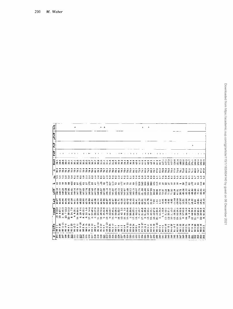
- * 20

5 206

207

208

209

21Q

211

212 -

213

214

215

216

217

218

219

220

221

222

223

224

225

226

227

228

229

230

231

232

233

234

235

236

237

238

239

240

241

242

243

244

245

246

247

248

249

250

251

252

253

254

255 -

DA

TE

89

3 1

90

3 26

89 1

1 21

89 10 6

86 4 5

85 2

23

84 12 3

834 1

1 85

10 18

86 3 14

885 15

85 1

26

83 3 10

88 5 7

85 12 10

85 3 27

81 9 3

88 12 20

88 6 26

85 3 10

88 5 7

88 7 6

88 1

2

88 5 8

88 12 21

88 4 19

80 9 24

90 6 5

83 10 8

81 1

1 27

88 1

1 5

90 5 1

1 89 6 16

86 6 19

89 I

1 25

83 4 4

84 4 5

88 6 10

83 12

1 94

4 26

81 10 7

82 6 20

89 1

25

88 6 24

90 2

21

596 18

51 9 14

90 3 25

90 8 26

89 9 16

90 3 3

TIM

E

13: 8:19.8

22: 8z57.1

2: 36:45.2

23: 7.12.3

22: 59:10.3

8. 24

: 7.9

4: 8:35.1

15: 34:55.5

4: 19: 6.4

8: 42:15.2

8: 22: 5.6

17. 41 14.4

0: 27:48.4

1: 22:17.6

11: 20:53.2

12: 48:12.4

5: 35:44.8

10: 18:38.l

9: 22:59.7

15: 27.45.4

1: 59.26.2

16: 31:32.7

12: 42:

2.5

22: 44: 2.5

10: 53:30.6

1: 56:30.6

17: 54:23.5

13: 42:51

1 7: 45~

26.7

17: 21:45.8

2: 51:36.8

13: 10:20.3

23. 42:35.1

18: 12:27.8

20: 14:35

0 2:

51:34.4

3: 1:33 8

11: 31 53.1

12: 22:21.5

10. 11.10.3

13: 19:ZO.l

23: 52:28.5

10: 14:33.6

8: 57:53.3

18: 20:14.6

14: 6.28.8

12: 44:29.8

21: 35:24.4

7: 53:45.3

23: 20:53.8

8: 41:44.3

LA

T

43.87

44.46

44.66

44.34

44.45

47.36

44.21

44.29

46.32

44.00

43.78

44.89

43.81

43.38

44.16

44.34

43.62

43.87

46.26

43.47

42.60

41.71

43.30

42.32

42.02

41.45

35.53

35.41

44.23

42.91

37.12

41.78

31.81

7.90

1.01

5.72

-6.85

-6.89

-6.80

-6 83

-11.44

-20.60

-27.97

10.21

16.90

17 76

18.32

9.59

19.65

16.51

16.13

LO

N

149.19

148.77

148.23

148.23

147.90

145.65

148.14

147.75

146.27

147.63

147.74

146 64

147.40

147.79

146.88

146.67

147.03

146.13

144.10

145.97

143.75

144.12

142.42

142 97

142.49

142.02

140.15

139.07

130.74

131 08

135.86

130.88

137.98

94.52

98.89

94.72

72.37

72.24

71.98

71 50

66.28

41.01

26.73

-60.56

-62.33

-68.81

-68.89

-84.66

-77.95

-93.65

-94.31 _

_

b 42

33

30

33

88

422

65

97

271

82

57

173

33

41

117

155

45

119

327

110

72

40

177

70

73

70

69

120

558

543

339

580

360

164

113

79

10

22

10

10

10

10

5 39

110

62

170

41

33

114

88

-

~

%A

5.4

80.2

5 0

79.4

5.5

79.2

5.0

79.4

5.4

79.2

5.4

75.9

6.5

79.5

5.8

79.3

6.0

77.0

5.8

79.6

5 5

79.8

5.4

78.4

6.3

79.6

5.4

80.2

5.4

79.2

6.0

18.9

6.7

79.7

5.4

79.2

5.3

76.4

5 4

79.5

6.2

79.4

5.3

80.3

6.1

78.3

5.2

79.4

5.3

79.5

5.1

79.8

6.0

84.1

5 4

83.7

5.8

72 9

5.9

74.1

5.3

80 9

5.8

74.8

6.0

86.3

6 0

79.7

5 1

87.6

6.7

81.3

5 4

76.9

5.6

76.9

5.4

76 6

6.1

164

6.0

77.6

5.5

74.4

5.4

78.1

6.1

70.6

6.0

66.9

6 0

70.5

60 70

1 5.7

86 8

5.9

87.2

5.5

87.8

5.8

74.7

~.

-

BA

Z

29.5

29.6

29.8

30.0

30.1

30.1

30.1

30.3

30.3

30.5

30.5

30.7

30.7

30.7

30.9

31.0

31.1

31.5

31.6

31.8

33.7

33.9

34 2

34.4

34.8

35.4

39.8

40.6

41.0

41.6

41.9

42.5

43 3

90.1

91.2

91.3

117.1

117.1

117 3

117 7

124.6

151.4

166.2

263.0

269.2

274 7

275

1 280.9

282.4

292 0

292.3

-

__

Dow



ecember 2021

p- and s-wave reflections from anomalies in the lowermost mantle

Documents