Ozone variability and long-term changes Michel Van Roozendael, BIRA-IASB

SCIAMACHY book

2

• 1928: start of CFC production

• 1971: 1st observation of CFC in the atmosphere (J. Lovelock)

• 1974: identification of O3 destruction potential by CFC: Rowland & Molina • 1995: Nobel prize in chemistry: F. Rowland, M. Molina & P. Crutzen, 1995

1990: 80% of stratospheric chlorine is of anthropogenic origin

Long term ozone depletion • Increasing anthropogenic emissions, since industrial

revolution, esp. CFCs since 1960 increasing concentrations of destructive radicals steady decrease of O3 on a global scale

• Recurrent spring-time ozone hole at the South pole • Seasonal ozone depletion in the North pole, strongly

modulated by dynamics

3

4

Nature, Vol. 315, 16 May 1985 • First alarming signs of O3

degradation were given in 1984 and 1985 based on Dobson measurements at Syowa and Halley Bay (since 1957)

• Ozone layer thins dramatically in the local spring down to ~ 100 DU

This phenomenon was not

expected !

Dr. Shigeru Chubachi at Ozone Commission meeting in Halkidiki (Sept 1984)

5

Evolution of average (monthly) O3 layer thickness between 1956 and 1986

in October

In Februari

6

7

When the first TOMS measurements were taken the drop in ozone levels in the stratosphere was so dramatic that at first the scientists thought their instruments were faulty… TOMS quickly confirmed the results from Farman et al., and the term Antarctic ozone hole entered popular language.

8

NASA Nimbus 7

Heterogeneous chemistry on PSCs

9

Martine De Mazière

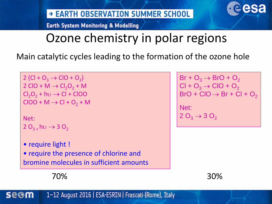
Ozone chemistry in polar regions Main catalytic cycles leading to the formation of the ozone hole 70% 30%

2 (Cl + O3 → ClO + O2) 2 ClO + M → Cl2O2 + M Cl2O2 + hυ → Cl + ClOO ClOO + M → Cl + O2 + M Net: 2 O3 + hυ → 3 O2 • require light ! • require the presence of chlorine and bromine molecules in sufficient amounts

Br + O3 → BrO + O2 Cl + O3 → ClO + O2 BrO + ClO → Br + Cl + O2 Net: 2 O3 → 3 O2

Experimental evidence

11

Antarctic Polar Air

Ozone (Scale at Left)

Reactive Chlorine (Scale at Right)

Latitude (Degrees South) 63 64 65 66 67 68 69 70 71 72

0

3000

2500

2000

1500

1000

500

1.5

0.5

1.0

0

Reac

tive

Chl

orin

e Ab

unda

nce

(P

arts

per

Bill

ion)

Ozo

ne A

bund

ance

(P

arts

per

Bill

ion)

Ozone and reactive chlorine measurements from a flight through the ozone hole in Antarctica, 1987

Examples of ozone depleting source gases (ODS)

12

Insert Fig 11.5 from [HW]

Situation 2004

13

14

Policies Scientific Assessments 1981 The Stratosphere 1981. Theory and Measurements. WMO No. 11 1985 Vienna Convention Atmospheric Ozone 1985. WMO No.16. 1987 Montreal Protocol 1988 International Ozone Trends Panel Report 1988.

Two volumes. WMO No. 18 1989 Scientific Assessment of Stratospheric Ozone: 1989.

Two volumes. WMO No. 20. 1990 London Adjustments and Amendment 1990 Climate Change, The IPCC first Scientific Assessment, Impacts Assessment and Response

Strategies Reports 1991 Scientific Assessment of Ozone Depletion: 1991.

WMO No. 25. 1992 Methyl Bromide: Its Atmospheric Science, Technology, and Economics (Assessment Supplement).

UNEP (1992). 1992 Copenhagen Adjustments and Amendment 1992 Rio de Janeiro Convention on Climate Change

IPCC Supplementary Report to the Scientific Assessment 1994 Scientific Assessment of Ozone Depletion: 1994. WMO No. 37

Climate Change 1994, Radiative Forcing of Climate Change and an Evaluation of the IPCC IS92 Emission Scenarios

1995 Vienna Adjustment 1995 Climate Change 1995. The IPCC second Scientific Assessment, Impacts Assessment …. Reports 1997 Montreal Adjustments and Amendment

Kyoto Protocol (UNFCCC third session, Kyoto, Dec. 1997) 1998 Scientific Assessment of Ozone Depletion: 1998. WMO. No. 44

1999 Beijing (China) Adjustments and Amendment 2000 The IPCC third Scientific Assessment, Impacts Assessment …. Reports 2002 Scientific Assessment of Ozone Depletion: 2002. WMO. No. 47 2007 Scientific Assessment of Ozone Depletion: 2006. WMO. No. 50 2007 The IPCC fourth Assessment Report: Climate Change 2007 2007 Montreal 19th meeting of the Parties: 191 countries agree to strengthen protection of the ozone layer by reducing HCFCs 2008 Doha 20th meeting of the Parties: Decision making on destruction ODS and funding phase-out HCFCs

2011 Scientific Assessment of ozone depletion: 2010. WMO No. 52 2013 The IPCC 5th assessment report 2014 Scientific Assessment of ozone depletion: 2014. WMO No. 55

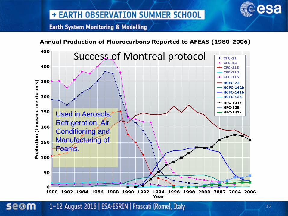
15

Used in Aerosols, Refrigeration, Air Conditioning and Manufacturing of Foams.

Success of Montreal protocol

Effect of Montreal Protocol

16

Max en 1997

Max en 2001

Reduction of chlorine and bromine in the stratosphere follows decrease of concentrations of the surface with a delay of 3 to 5 years = time to reach from troposphere stratosphere.

F. Hendrick, IASB

Max in 2001

Max in 1997

fits were applied to these data sets (black curves) to provide trends estimates. E. Mahieu, U. Liège

Most ODS are also greenhouse gases!

17

01000200030004000500060007000800090001000011000

Global Worming Potential (20 Year, CO2 = 1)(Source: Scientific Assessment of Ozone Depletion)

0.022

0.055

0.065

0.1

0.11

0.6

0.6

0.8

1

1

1

1.1

3

10

0 1 2 3 4 5 6 7 8 9 10 11

HFC-134a

HFC-32

HCFC-124

HCFC-22

HCFC-142b

Methyl Chloroform

HCFC-141b

Methyl Bromide

CFC-115

CFC-113

CFC-11

CFC-114

CFC-12

Carbon Tetrachloride

Halon-1211

Halon-1301

Ozone Depletion Potential (CFC-11 = 1)(Source: The Montreal Protocol)

Montreal Protocol has been beneficial for our climate Challenge: search for CFC substitutes that have a negligible GWP !

Success of the Montreal Protocol

18

The impact of the Montreal Protocol on climate is of order 5-6 times larger than the objectives of the Kyoto Protocol 2008-2012 !

Reduction by Montreal Protocol of ~12 GtCO2-eq/yr

Monitoring of the ozone hole using satellites and models

19

20 Antarctic O3 Bulletin 2011

Ozone mass deficit averaged over the 60 consecutive worst days.. The plot is produced at WMO based on data from NASA. The NASA data have some gaps in the mid 1990s, but this does not affect the ranking of the 2015 ozone hole..

Area of the ozone hole for the years 1979-2015, averaged over the 60 consecutive worst days. The plot is produced at WMO, based on data from NASA. The NASA data have some gaps in the mid 1990s, but this does not affect the ranking of the 2015 ozone hole.

Evolution of ozone hole area: South Pole

http://www.wmo.int/pages/prog/arep/gaw/ozone/

Evolution of the Spring polar ozone over the North Pole from 1979 until 2011

21

MACC/MSR, KNMI

March monthly mean assimilated total ozone

22

Most severe Arctic Ozone Hole: 2010-2011

23

What would have happened to the ozone layer if chlorofluorocarbons (CFCs) had not been regulated?

24

Newman et al., ACP, 2009

Current situation • O3 in the middle latitude:

– 6% (3.5%) lower than average in 1964-1980 SH (NH) – UV has not increased since the late 1990s

• O3 hole at the poles is still as in early 1990 (subject variability) i.e. in Antarctica in October, 40% lower than in 1980

• UV on Antarctic is higher by 55 to 85% than in 1963-1980

• Evidences for changes in SH tropospheric summertime circulation due to Antarctic ozone hole

• The stratosphere has cooled a few K between 1980 and 1995 due to ozone depletion; the cooling reinforced by increasing GHG esp. in recent years

25

Ref: WMO O3 Assessment, 2014

Coupling between ozone and climate • Concentrations of greenhouse gases (CO2, CH4, N2O,...) rise • T°rises at the surface; but decreases in the stratosphere • Atmospheric transport changes, rate of chemical reactions

changes • Frequency of formation of clouds, aerosols and PSC

change • Radiation balance changes • Ozone formation / degradation is influenced, in turn

ozone affects UV, T°stratosphere ....

26

Future evolution of ODS

27

• EESC back to 1980 levels: in ~2050 in ~2065 at the poles

(older air)

Future evolution of mid-latitude ozone

28

Average total column ozone changes over the same period, from multiple model simulations compared with observations between 1965 and 2013. Four possible greenhouse gas (CO2, CH4, and N2O) futures are shown. The four scenarios correspond to +2.6 (purple), +4.5 (green), +6.0 (brown), and +8.5 (red) W m-2 of global radiative forcing

WMO-2014

Impact of projected changes in GHGs on ozone • Increased CO2, CH4 and N2O

cools the stratosphere, which tends to increase O3 because of temperature-dependent chemistry (reduced efficiency of loss)

• Increased CH4 and N2O also have further chemical impact on O3

– CH4 increases O3 by mitigating the effect of halogen-driven O3 destruction catalytic cycles

– N2O decreases O3 through enhancing the efficiency of the NOx-driven catalytic cycles

29

Evidence for O3 recovery in upper stratosphere

O3 recovery at 45 km altitude is due to combination of reduction in ODS (Montreal protocol) reinforced by cooling due to GHG increase

30

1979-1997 2000-2013

Regional ozone trend analysis

31

• Regional trends in total ozone estimated from harmonised multi-sensor satellite data set (1995-2013)

• Trends in middle latitudes still not significant; recovery masked by natural variability; additional 5-10 years of observations are required

Coldewey-Egbers et al., GRL, 2015

3 Fingerprints of Ozone Hole recovery

32

30 June 2016 release

(i) increases in ozone column amounts

Solomon et al., 2016

33

Syowa South Pole

1980-2000 2000-2015

(ii) changes in the vertical profile of ozone concentration

34

(iii) decreases in the areal extent of the ozone hole

Ozone hole area Day ozone hole area > 12 million km2

Predicted reduction of the tropical ozone layer Recent evidence for changes in tropical upwelling and higher latitudes downwelling due to climate change Impact on ozone distribution

35

T°↑

T°↓

WMO-2014

Impact of rising GHG on tropical ozone

36

Upper stratosphere

Mid-stratosphere

Troposphere Meul et al., GRL, 2016

Conclusion: Mid-strat ozone decrease due to change in circulation (partly) compensated by increases to chemical effects at other altitudes

37

Meul et al., GRL, 2016

Impact on UVB irradiance

Summary • O3 on a global scale will return to state from 1980 by 2050, i.e. faster than ODS,

namely: – Around 2030-2040 in middle latitudes of both hemispheres – Around 2045-2060 in Antarctica – The increase of ozone will be accelerated in a colder stratosphere under the

impact of GHGs • As result, at the end of the 21st century the stratospheric ozone concentration

will be higher than in 1980 • Tropical ozone might decrease due to climate-change induced changes in the

Dobson-Brewer circulation

• Large uncertainties in future emission scenarios and resulting impacts

38

39