applied sciences

Article

Ownership Cost Comparison of Battery Electric andNon-Plugin Hybrid Vehicles: AConsumer Perspective

Lawrence Fulton ID

Department of Health Administration, Texas State University, San Marcos, TX 78666, USA; lf25@txstate.edu

Received: 23 July 2018; Accepted: 27 August 2018; Published: 29 August 2018�����������������

Abstract: This study evaluates eight-year ownership costs for battery electric vehicles (BEV) versusnon-plugin hybrid vehicles, using forecasting to estimate future electricity and conventional gasolineprices and incorporating these in a multiple design of experiments simulation. Results suggest thatwhile electric vehicles are statistically dominant in terms of variable costs over an 8-year life-span,high-performance hybrid non-plugins achieve variable fuel costs nearly as good as low-performingelectric vehicles (those attaining only 3 miles per kilowatt hour) and that these hybrid acquisitioncosts are (on average) lower, yet the vehicles retain higher residual values. In general, the sixsmallest ownership costs are split evenly between hybrid and electric vehicles; however, inflation forconventional regular gasoline is estimated to outstrip inflation per kilowatt hour. Thus, non-pluginhybrid cars are likely to require considerably more advanced engineering to keep pace.

Keywords: BEV; ownership cost analysis; design of experiments; forecasting; monte carlo simulation

1. Introduction

With more constraints on energy resources, coupled with stringent regulations due to fossilfuel pollution, the growth of energy efficient technologies and clean, renewable energy sources isessential for ensuring sustainable practices. When assessing the potential gains from energy efficienttechnologies, engineering efficiency analysis must consider both the scale of energy flow and thetechnical component for improvement. As part of this analysis, the industry must thoroughlyevaluate and compare the costs and demand trade-offs from a consumer perspective to ensure that theengineering of sustainable products provides optimal consumer satisfaction [1].

With volatility of gasoline prices, the purchase of electric cars has become an attractive option tosome, but understanding the actual ownership costs associated with such a purchase requires analysis.Acquisition costs must take into consideration tax credits, while variable fuel costs associated withelectric vehicles should be based on the cost per kilowatt hour, usage, and other factors. Further,maintenance and residual value must be investigated to paint a complete picture of life-cycle costsfrom consumers’ perspectives.

Some work has been done in the area of ownership and life-cycle costs for vehicles, but thearea is relatively new [2]. Delucchi & Lipman addressed the issue of lifecycle costs by developinga detailed model of the performance, energy use, manufacturing cost, retail cost, and lifecycle cost ofbattery-powered vehicles and comparable gasoline-powered vehicles [3]. They found in their 2001study that for electric vehicles to be cost-competitive with gasoline-powered vehicles, batteries musthave a lower manufacturing cost, as well as a longer battery life. The work provides a reasonableframework for an updated study. In another dated (2006) study, Lipman & Delucchi developeda vehicle simulation cost model to analyze the manufacturing costs, retail prices, and lifecyclecosts of hybrid gasoline-electric vehicles, conventional vehicles, electric-drive vehicles, and other

Appl. Sci. 2018, 8, 1487; doi:10.3390/app8091487 www.mdpi.com/journal/applsci

Appl. Sci. 2018, 8, 1487 2 of 14

alternative-fuel vehicles [4]. Due to its date, it lacks relevance based on the speed of technologicalchange. Silva, Ross & Farias contributed to the worldwide methodology for the calculation offuel consumption and emission factors when regarding emission standards, with distinct drivingstyles [5]. Using this methodology, they simulated the energy consumption, emissions, and cost ofplug-in hybrid vehicles. Their work provides a good framework for cost estimation, but focusesonly on plug-in hybrids. Werber, Fischer & Schwartz compared the lifecycle costs of electric cars tosimilar gasoline-powered vehicles under different scenarios of required driving range and cost ofgasoline [6]. They found that the electric cars with approximately 150 km range are a technologicallyviable, cost competitive, high performance, high efficiency alternative that can presently suit the vastmajority of consumers’ needs. This study uses similar methods. Weiller developed a simulationalgorithm to explore the effects of different charging behaviors of plug-in hybrid electric vehicles(PHEVs) on electricity demand profiles and energy use, in terms of time of day and location (at home,the workplace, or public areas) [7]. The study focused on electrical demand of PHEVs, but diddemonstrate consumption of 1.5–2.0 kWh per day when electric chargers were available in the home.Ernst et al. introduce a total cost of ownership model for the average car user in Germany to comparethe energy consumption of a conventional vehicle versus a plug-in hybrid electric vehicle [8]. Thisdated study found a break-even time frame of six years with 4 kWh batteries. Many studies have foundthat electric vehicles might be cheaper or more expensive than combustion engine vehicles dependingon assumptions [9,10]. No studies compared solely battery electric vehicles (BEV) vs. PHEV vehicles.

Lieven et al. conducted a study forecasting the market potential of electric vehicles by analyzingboth individual priorities and barriers due to social preferences [11]. Using a mixed multiple discrete-continuous extreme value model approach, Shin et al. investigated how the introduction of electricvehicles may influence the usage of existing cars. Additionally, they used a survey of 250 households toanalyze a future automobile market that includes electric vehicles, taking into account the heterogeneityof consumer preferences and usage patterns [12]. He, Chen & Conzelmann analyzed the vehicleusage and consumer profile attributes extracted from both National Household Travel Survey andVehicle Quality Survey data to understand the impact of vehicle usage upon consumers’ choices ofhybrid vehicles in the United States [13]. Kelly, MacDonald & Keoleian studied the impacts thatplug-in hybrid electric vehicles can have on energy consumption and related emissions, as they aredependent on vehicle technology, driving patterns, and charging behavior. Moreover, they developeda methodology to simulate charging and gasoline consumption based on driving pattern data in theNational Household Travel Survey, examining the effects of charging location, charging rate, time ofcharging, and battery size [14]. Ozdemir & Hartmann calculate the energy consumption shares ofplug-in hybrid vehicles for electricity from the grid and conventional fuel by determining the optimalelectric driving range for different oil price levels [15]. In an interesting paper, Ahmadi, Cai & Khannaused optimization models to suggest that hybrid vehicles were generally better when considering totallife-cycle costs, under the assumption that miles traveled per day were high [16]. This detailed papergeneralized overall vehicle classifications but did not use lifecycle forecasts for energy costs or useresidual costs (a consumer perspective). In another good study, Palmer et al. used panel regression tocompare life-cycle costs for four separate sites, but did not calculate forecasts for energy costs, did notconsider the effects of seasonal differences, and used vehicle data from 2016. Their study also focusedon four specific locations, rather than the U.S en toto [17].

The problem of interest is a comparison of the life-cycle costs of electric vs. hybrid vehicles formthe consumer perspective. This study examines the engineering trade-off considerations of averagemiles per gallon (mpg) versus average miles per kilowatt hour (mpkWh) when considering cost forboth gasoline and retail grid power. The research question for this study is then straightforward: Whatare the estimated life-cycle costs associated with the purchase of either an electric or hybrid vehiclein 2018? This research question addresses engineering efficiency trade-off considerations that mightbe reasonably assessable given fuel and electricity forecasting models. This may be the first study

Appl. Sci. 2018, 8, 1487 3 of 14

to compare specifically electric and hybrid vehicles based on known 2018 engineering capabilities,as well as time series forecasts of energy costs.

2. Materials and Methods

2.1. Study Design, Setting, & Data

This study leverages 23 years of data from the U.S. Department of Energy on average price perkilowatt hour [18], average dollars per gallon for regular conventional gasoline [19], the distribution ofvehicle miles driven per year [20], base manufacturer suggested retail prices (MSRP) [21], maintenancefactors, insurance estimates, and simulation with design of experiments parameters to investigatelife-cycle costs for electric and non-plugin hybrid vehicles. The study also includes time seriesforecasts for cents per kilowatt hour (cpkWh) and dollars per gallon to use in simulating an 8-yearvehicle lifespan. While vehicles may last longer, the average length of ownership is approximately6.5 years [22]. Further, electric battery warranties are often only 8 years [23].

The study includes base MSRP data as acquisition costs and forecasting of both cpkWh and centsper gallon of regular gasoline to estimate ownership costs. Maintenance is accounted for by applying3.5 cents per mile for electric vehicles and 6 cents per mile for hybrids, although this is imprecise [24].Insurance costs may be higher or lower depending on car value and insurance company, so a fixedvalue of 5% based on initial cost of the car is assigned. Electric vehicles depreciate at a more rapid ratethan hybrid vehicles [25]. Over four years, gasoline cars retained on average 45% of their value, whileelectric vehicles just above 25% after adjustment for any Federal tax credit. It is unknown what thedepreciation on new cars will be after an 8-year lifespan will be; however, it is assumed that the decayover the next four years will match the previous four, 0.45 remaining × 0.65 decay rate = 0.29 residualfor gasoline cars and 0.25 remaining × 0.75 decay rate = 0.19 for electric cars.

The setting for this study is the entirety of the United States, although the analysis is readilyparsed to any individual state for which data are gathered. For generalization, all coding is provided.Data sources for costs derive primarily from the U.S. Department of Energy.

2.2. Simulation Sets, Parameters, Stochastic Variables, Deterministic Variables, Formulae, and Flowcharts

Sets. Three index sets are used in the simulation. The first index, i, counts the number of simulationiterations, i = {1, 2, . . . , 25} (see Simulation Iterations under results). The second index, t, counts theday of the year, t = {1, 2, . . . , 365}. The third index, y, counts the number of years in the simulation,y = {1, 2, . . . , 8}.

Design of Experiments Parameters. The simulation leverages design of experiments (DOE)parameters that include miles per kilowatt hour (mpKh) design factor and miles per gallon (mpg)for gasoline powered cars. Daily miles driven is included as a probability distribution. Cost in centsper kilowatt hour (cpkWh) and in cents per gallon of fuel are forecasted as explicated in the resultssection for each month in the simulation, and those monthly estimates are applied to each day withinthe month. All DOE parameters are investigated within reasonable ranges as demonstrated throughanalysis of datasets.

The parameter range of mpkWh for new electric cars derived from an analysis of EVadoption [26].The distribution of interest was the daily mpkWh because it provides a mechanism for assessingcomparative efficiency of vehicles when coupled with a time series analysis of cost per kWh.The minimum efficiency for 2018 electric cars based on distance and battery size is 2.89 mpKh (TeslaModel X P1000, Palo Alto, CA, USA), and the maximum is 4.43 mpKh for the Hyundai Ioniq Electric,Seoul, South Korea. Thus, the DOE parameter is fixed simplistically within the range of 3 to 5 torepresent a feasible engineering range.

The hybrid vehicle mpg parameter was evaluated using top 10, highest MPG hybrid vehiclesprovided by Fueleconomy.gov [27]. Due to mpg ties, there are actually 11 vehicles on this list.Gas mileage for these hybrid vehicles ranges from 46 mpg (Toyota Prius, Toyota, Aichi, Japan) to

Appl. Sci. 2018, 8, 1487 4 of 14

58 mpg (Hyundai Ioniq, Seoul, South Korea). Given this range, the DOE parameter for mpg was setwithin the range of 40 to 60.

Stochastic Variable. Miles driven annually depends on many factors; however, Department ofTransportation (DoT) provides average data on its website [28]. On average, drivers drove 13,476 milesannually in 2017, or approximately 37 miles per day. The variability is high among income groupsand age groups [20]. Due to the high variability associated with driving vehicles, the study assumesa right-skewed exponential distribution centered at 37 miles.

Deterministic Estimates. Estimates of the daily cost per kilowatt hour ($/kWh) and cost per gallon($/gl) are the primary deterministic components. These are estimated using forecasting techniquesexplicated in the Results section.

Formulae. The primary equations calculate variable costs for both the electric and the hybridautomobile options. For each iteration, day, year, and DOE parameter, the following equationsare calculated.

Ce =$

kWh× kWh

mile× Dt (1)

Ch =$

gallon× gallons

mile× Dt (2)

The simulation flowchart is shown in Figure 1. For each of the iterations, the DOE parameters areset, driving distance is sampled, and costs for each vehicle are estimated for an 8-year vehicle lifespan.

Appl. Sci. 2018, 8, x FOR PEER REVIEW 4 of 14

Stochastic Variable. Miles driven annually depends on many factors; however, Department of Transportation (DoT) provides average data on its website [28]. On average, drivers drove 13,476 miles annually in 2017, or approximately 37 miles per day. The variability is high among income groups and age groups [20]. Due to the high variability associated with driving vehicles, the study assumes a right-skewed exponential distribution centered at 37 miles.

Deterministic Estimates. Estimates of the daily cost per kilowatt hour ($/kWh) and cost per gallon ($/gl) are the primary deterministic components. These are estimated using forecasting techniques explicated in the Results section.

Formulae. The primary equations calculate variable costs for both the electric and the hybrid automobile options. For each iteration, day, year, and DOE parameter, the following equations are calculated. = $ ℎ × ℎ × (1)

= $ × × (2)

The simulation flowchart is shown in Figure 1. For each of the iterations, the DOE parameters are set, driving distance is sampled, and costs for each vehicle are estimated for an 8-year vehicle lifespan.

Figure 1. Simulation Flowchart.

After the simulation is run over the nine possible DOE combinations, the results are then coupled with fixed-cost estimates of maintenance (per type of vehicle), estimates for insurance, and estimated residual values to generate a total cost of ownership picture for specific vehicles in the study.

3. Results

3.1. Descriptive Statistics

The analysis of results begins with variable costs. Table 1 provides the pure electric car range in miles per kWh for available U.S. battery electric vehicles [26]. Smart ForTwo was eliminated from

Estimate Driving Distance (Dt) on Day t based on

DoT distribution, D~exp(1/37)

Forecast daily $/kWh and $/gallon based on

forecasts (see Results section)

Calculate daily cost for battery electric vehicle option

Cht=(kWh / m) x ($ / kWh) x Dt

Start

Set DOE parameters for experimental run:

mpkWh [1, 2, 3] and mpg [40, 50, 60]

t<365 days?

y<8 years?

End

yes

yes

no

no

Set seed. Initialize indices: run number i =1, day number t=1

year number y, y=1

i < 25

no

yes

Calculate daily cost for non-plugin hybrid:

Cet=(gl / m) x ($ / gl) x Dt

y=y+1Increment

Year

y=y+1Increment

Year

t=t+1Increment

day

Setsi=iteration, {1, 2,..25}(See Simulation iterations)t=day, {1, 2, ..365} y=year, {1, 2, .. 8}

Design of Experiments ParametersmpkWh= {1, 2, 3}mpg= {40, 50, 60}

Stochastic DistributionDt=daily driving distance

Deterministic Estimates$/kWht: dollars per kilowatt hour$/gallont: dollars per gallon

FormulaeCet: daily cost for BEVCht: daily cost for non-plugin hybrid

Figure 1. Simulation Flowchart.

After the simulation is run over the nine possible DOE combinations, the results are then coupledwith fixed-cost estimates of maintenance (per type of vehicle), estimates for insurance, and estimatedresidual values to generate a total cost of ownership picture for specific vehicles in the study.

3. Results

3.1. Descriptive Statistics

The analysis of results begins with variable costs. Table 1 provides the pure electric car rangein miles per kWh for available U.S. battery electric vehicles [26]. Smart ForTwo was eliminated from

Appl. Sci. 2018, 8, 1487 5 of 14

this list due to its limited range (58 miles). The average mpkWh is 3.56, and the median is 3.50.The standard deviation is quite small, at 0.38. The median base manufacturer suggested retail price(MSRP) for new electric vehicles is $35,000. Tesla models largely affect the mean ($56,920.71) [21].

Table 1. This table provides the range per kWh of currently available fully electric vehicles used in thestudy, along with the base manufacturer suggested retail prices (MSRP).

Manufacturer Make Range in Miles kWh Battery Pack Miles/kWh MSRP Base

BMW i3 114 33 3.45 $44,450.00Fiat 500e 87 24 3.63 $32,995.00Ford Focus Electric 115 33 3.48 $29,120.00

Chevrolet Bolt EV 238 60 3.97 $36,620.00Honda Clarity Electric 89 25.5 3.49 $33,400.00

Hyundai Ioniq Electric 124 28 4.43 $29,500.00Kia Soul EV 111 30 3.70 $32,250.00

Nissan Leaf 107 30 3.57 $29,990.00Tesla Model 3 310 78 3.97 $35,000.00Tesla Model S 75D 275 75 3.67 $74,500.00Tesla Model S 100D 351 100 3.51 $94,000.00Tesla Model S P100D 337 100 3.37 $135,000.00Tesla Model X 75 237 75 3.16 $70,532.00Tesla Model X 100D 295 100 2.95 $96,000.00

Model XP100 Model X P100D 289 100 2.89 $140,000.00VW e-Golf 125 35.8 3.49 $30,495.00

Table 2 illustrates the comparison group, hybrid electric vehicles (non-plugin). This groupconsists of Fueleconomy.gov’s top 10 vehicles (11 listed due to mpg ties), all of which are 4 cylinderautomatics [27]. The average mpg for hybrid vehicles in the study is 50.64 mpg, with a median of50.00 mpg and a standard deviation of 4.31 mpg. The median MSRP is $23,475, with a mean of$24,865 [21].

Table 2. This table illustrates the non-plugin hybrid vehicles included in the study and their associatedestimated miles per gallon.

Make Model Engine Size(All 4 Cylinder Automatics) Estimated mpg MSRP

Hyundai Ioniq Blue 1.6 L 58 $22,200.00Toyoto Prius Eco 1.8 L 56 $25,165.00Hundai Ioniq 1.6 L 55 $22,000.00Toyota Camry Hybrid LE 2.5 L 52 $27,950.00Toyota Prius 1.8 L 52 $23,475.00

Kia Niro FE 1.6 L 50 $23,340.00Kia Niro 1.6 L 49 $23,340.00

Honda Accord Hybrid 2.0 L 47 $25,100.00Chevrolet Malibu Hybrid 1.8 L 46 $27,920.00

Toyota Camry Hybrid LXE 2.5 L 46 $32,400.00Toyota Prius c 1.5 L 46 $20,630.00

The nation-wide average price per gallon of regular conventional gasoline for the United Statesrose from $1.11 in January of 1995 to $2.77 as of April 2018 [19]. During the same span of time, themean cost per kWh for electricity increased from 0.0785 cents to 0.1289 cents.

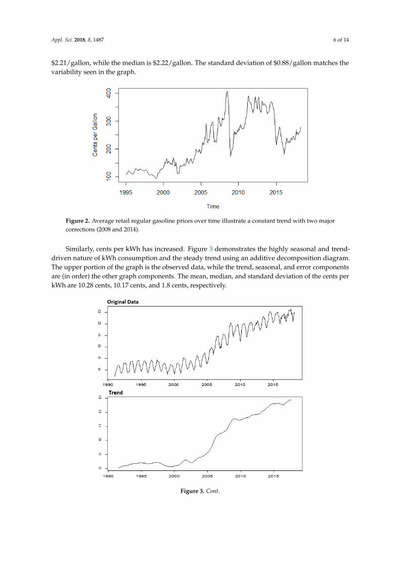
As depicted in Figure 2, retail regular gasoline prices rose fairly consistently through 2008 andthen experienced a precipitous drop, perhaps due to the economic slowdown [29]. They then roseagain until 2014 prior to another major downward adjustment, perhaps due to OPEC ineffectivenessas a cartel, as well as the laws of supply and demand [30]. The mean gas price over this time is

Appl. Sci. 2018, 8, 1487 6 of 14

$2.21/gallon, while the median is $2.22/gallon. The standard deviation of $0.88/gallon matches thevariability seen in the graph.

Appl. Sci. 2018, 8, x FOR PEER REVIEW 6 of 14

As depicted in Figure 2, retail regular gasoline prices rose fairly consistently through 2008 and then experienced a precipitous drop, perhaps due to the economic slowdown [29]. They then rose again until 2014 prior to another major downward adjustment, perhaps due to OPEC ineffectiveness as a cartel, as well as the laws of supply and demand [30]. The mean gas price over this time is $2.21/gallon, while the median is $2.22/gallon. The standard deviation of $0.88/gallon matches the variability seen in the graph.

Figure 2. Average retail regular gasoline prices over time illustrate a constant trend with two major corrections (2008 and 2014).

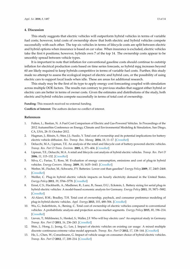
Similarly, cents per kWh has increased. Figure 3 demonstrates the highly seasonal and trend-driven nature of kWh consumption and the steady trend using an additive decomposition diagram. The upper portion of the graph is the observed data, while the trend, seasonal, and error components are (in order) the other graph components. The mean, median, and standard deviation of the cents per kWh are 10.28 cents, 10.17 cents, and 1.8 cents, respectively.

Figure 2. Average retail regular gasoline prices over time illustrate a constant trend with two majorcorrections (2008 and 2014).

Similarly, cents per kWh has increased. Figure 3 demonstrates the highly seasonal and trend-driven nature of kWh consumption and the steady trend using an additive decomposition diagram.The upper portion of the graph is the observed data, while the trend, seasonal, and error componentsare (in order) the other graph components. The mean, median, and standard deviation of the cents perkWh are 10.28 cents, 10.17 cents, and 1.8 cents, respectively.

Appl. Sci. 2018, 8, x FOR PEER REVIEW 6 of 14

As depicted in Figure 2, retail regular gasoline prices rose fairly consistently through 2008 and then experienced a precipitous drop, perhaps due to the economic slowdown [29]. They then rose again until 2014 prior to another major downward adjustment, perhaps due to OPEC ineffectiveness as a cartel, as well as the laws of supply and demand [30]. The mean gas price over this time is $2.21/gallon, while the median is $2.22/gallon. The standard deviation of $0.88/gallon matches the variability seen in the graph.

Figure 2. Average retail regular gasoline prices over time illustrate a constant trend with two major corrections (2008 and 2014).

Similarly, cents per kWh has increased. Figure 3 demonstrates the highly seasonal and trend-driven nature of kWh consumption and the steady trend using an additive decomposition diagram. The upper portion of the graph is the observed data, while the trend, seasonal, and error components are (in order) the other graph components. The mean, median, and standard deviation of the cents per kWh are 10.28 cents, 10.17 cents, and 1.8 cents, respectively.

Figure 3. Cont.

Appl. Sci. 2018, 8, 1487 7 of 14Appl. Sci. 2018, 8, x FOR PEER REVIEW 7 of 14

Figure 3. The additive decomposition of cents/kWh illustrates the significant trend and seasonal components of the time series.

Spearman’s correlation between the cost per gallon (cents) and the cents/kWh is positive and strong (ρ = 0.787, p < 0.001). Fitting a linear model suggests that the price per kWh increases at 81% of the rate that price per retail conventional gasoline increases.

3.2. Forecasts

While the Annual Energy Outlook from the Energy Information Administration provides forecasts for gasoline and electrical consumption, the data are provided annually for dollars per one million British Thermal Units ($/MBtu) through 2050, which ignores the seasonality and is less useful for consumers [31]. Figure 4 is a graph for 2018–2026 from the Annual Energy Outlook.

Figure 4. Energy price forecasts from the U.S. Energy Information Administration in $/MMBtu.

Figure 3. The additive decomposition of cents/kWh illustrates the significant trend and seasonalcomponents of the time series.

Spearman’s correlation between the cost per gallon (cents) and the cents/kWh is positive andstrong (ρ = 0.787, p < 0.001). Fitting a linear model suggests that the price per kWh increases at 81% ofthe rate that price per retail conventional gasoline increases.

3.2. Forecasts

While the Annual Energy Outlook from the Energy Information Administration provides forecastsfor gasoline and electrical consumption, the data are provided annually for dollars per one millionBritish Thermal Units ($/MBtu) through 2050, which ignores the seasonality and is less useful forconsumers [31]. Figure 4 is a graph for 2018–2026 from the Annual Energy Outlook.

Appl. Sci. 2018, 8, x FOR PEER REVIEW 7 of 14

Figure 3. The additive decomposition of cents/kWh illustrates the significant trend and seasonal components of the time series.

Spearman’s correlation between the cost per gallon (cents) and the cents/kWh is positive and strong (ρ = 0.787, p < 0.001). Fitting a linear model suggests that the price per kWh increases at 81% of the rate that price per retail conventional gasoline increases.

3.2. Forecasts

While the Annual Energy Outlook from the Energy Information Administration provides forecasts for gasoline and electrical consumption, the data are provided annually for dollars per one million British Thermal Units ($/MBtu) through 2050, which ignores the seasonality and is less useful for consumers [31]. Figure 4 is a graph for 2018–2026 from the Annual Energy Outlook.

Figure 4. Energy price forecasts from the U.S. Energy Information Administration in $/MMBtu. Figure 4. Energy price forecasts from the U.S. Energy Information Administration in $/MMBtu.

Appl. Sci. 2018, 8, 1487 8 of 14

To facilitate decision-making over the life-span of a vehicle, an 8-year horizon for gasoline andkWh costs was estimated using error/trend seasonality (ETS) and auto-regressive integrated movingaverage (ARIMA) models. The best performing models for both kWh and gasoline prices based onthe mean absolute scaled error (MASE, a ratio of the model’s mean absolute error divide by the meanabsolute error of a seasonal naïve model) were used for forecasting. The MASE provides a comparativemetric of forecasting performance by leveraging a model’s performance versus a seasonal naïve model.Values of MASE less than 1 indicate model performance better than the seasonal naïve [32].

The “ets” and “auto.arima” functions [32] in [33] were used on both the price per kWh and theprice per gallon of gas. For both variables, ETS models proved to have the best accuracy based on MASEscores when predicting a 20% validation set. When using the entirety of the data, the model selectedfor price per kWh was a Holt-Winter’s ETS (smoothed error, trend, and seasonality components) withmultiplicative error, additive trend, and additive seasonality components. The resulting MASE was0.36, indicating a far superior performance to the seasonal naïve model. The model selected for theprice per gallon of gasoline was another Holt-Winter’s ETS with multiplicative error, additive trend,and multiplicative error. The MASE was 0.23, far superior to a seasonal naïve model. Table 3 depictsthe metrics for both variables and the optimized ETS and ARIMA models.

Table 3. The accuracy metrics for the forecast models are shown below. ME is the mean error (a measureof bias), RMSE is the root mean squared error (a measure of variability), MAE is the mean absolute error(a measure of variability), MPE is the mean percent error (a measure of bias), MAPE is the mean absolutepercent error (a measure of variability), and MASE is the mean absolute scaled error (a comparativemeasure of performance versus the seasonal naïve with lower values meaning better performance.

ME RMSE MAE MPE MAPE MASE

ETS Gasoline 0.450 13.096 8.538 0.082 3.835 0.235ARIMA Gasoline 0.666 12.689 8.802 0.220 3.881 0.242

ETS kWh 0.004 0.133 0.102 0.043 0.990 0.355ARIMA kWH 0.003 0.134 0.103 0.043 0.995 0.358

Forecasts using these models were generated for eight-years, which is quite a long forecastgenerating large error bands. Figure 5 illustrates both forecasts. Each of the 8 year × 12 month = 96forecasts for each variable are used to feed the simulation model.

Appl. Sci. 2018, 8, x FOR PEER REVIEW 8 of 14

To facilitate decision-making over the life-span of a vehicle, an 8-year horizon for gasoline and kWh costs was estimated using error/trend seasonality (ETS) and auto-regressive integrated moving average (ARIMA) models. The best performing models for both kWh and gasoline prices based on the mean absolute scaled error (MASE, a ratio of the model’s mean absolute error divide by the mean absolute error of a seasonal naïve model) were used for forecasting. The MASE provides a comparative metric of forecasting performance by leveraging a model’s performance versus a seasonal naïve model. Values of MASE less than 1 indicate model performance better than the seasonal naïve [32].

The “ets” and “auto.arima” functions [32] in [33] were used on both the price per kWh and the price per gallon of gas. For both variables, ETS models proved to have the best accuracy based on MASE scores when predicting a 20% validation set. When using the entirety of the data, the model selected for price per kWh was a Holt-Winter’s ETS (smoothed error, trend, and seasonality components) with multiplicative error, additive trend, and additive seasonality components. The resulting MASE was 0.36, indicating a far superior performance to the seasonal naïve model. The model selected for the price per gallon of gasoline was another Holt-Winter’s ETS with multiplicative error, additive trend, and multiplicative error. The MASE was 0.23, far superior to a seasonal naïve model. Table 3 depicts the metrics for both variables and the optimized ETS and ARIMA models.

Table 3. The accuracy metrics for the forecast models are shown below. ME is the mean error (a measure of bias), RMSE is the root mean squared error (a measure of variability), MAE is the mean absolute error (a measure of variability), MPE is the mean percent error (a measure of bias), MAPE is the mean absolute percent error (a measure of variability), and MASE is the mean absolute scaled error (a comparative measure of performance versus the seasonal naïve with lower values meaning better performance.

ME RMSE MAE MPE MAPE MASE ETS Gasoline 0.450 13.096 8.538 0.082 3.835 0.235

ARIMA Gasoline 0.666 12.689 8.802 0.220 3.881 0.242 ETS kWh 0.004 0.133 0.102 0.043 0.990 0.355

ARIMA kWH 0.003 0.134 0.103 0.043 0.995 0.358

Forecasts using these models were generated for eight-years, which is quite a long forecast generating large error bands. Figure 5 illustrates both forecasts. Each of the 8 year × 12 month = 96 forecasts for each variable are used to feed the simulation model.

Figure 5. Forecasts for cents/kWh and cents/gallon of gasoline for the best error/trend seasonality (ETS) models are shown. The large forecast period results in error bands being wide. Figure 5. Forecasts for cents/kWh and cents/gallon of gasoline for the best error/trend seasonality(ETS) models are shown. The large forecast period results in error bands being wide.

Appl. Sci. 2018, 8, 1487 9 of 14

3.3. Daily Driving Distribution

Daily driving distance should logically be restricted within certain bounds based on an analysisof driving characteristics of US drivers. The US Department of Transportation statistics suggest that 37miles per day per driver is likely a good center estimate (US Department of Transportation, 2018 #42).This value is largely confirmed by the 2016 American Survey of Drivers conducted by the AutomobileAssociation of America [34]. The distribution is therefore skewed. To account for large variations andprobable right skew (the distribution is truncated at zero), daily driving distance is modeled as anexponential distribution with λ = 37.

3.4. Simulation Iterations

The number of simulation runs was set to 25. This number of runs resulted in maximum standarderrors of less than one cent for both the electric car and hybrid car analyses. For electric cars, theassociated standard errors for 25 runs were {0.60, 0.45, 0.36} cents for {3, 4, 5} mpkWh runs. For hybridcars, the standard errors for 25 runs were {0.93, 0.74, 0.62} cents for {40, 50, 60} mpg runs.

3.5. Verification and Validation

All parameters were recorded in a csv file and checked for appropriateness. Descriptive statisticshelped to ensure that values were appropriate. The simulation produced an average daily drivingdistance of 36.3 miles, which is to be expected given that the mean of the a priori exponentialdistribution was 37. Other components of the simulation were based on DOE parameters or forecasts,which are fixed.

To be valid for comparison, we needed to ensure that the random streams were identicalacross experimental conditions for the stochastic distribution of miles driven. To do so, we useda Mersenne-Twister and a common pseudo-random distance for each 8-year, 365-day run. Only oneset of random exponentials was produced for all 8 years and 365 days runs to ensure that changes inDOE factors would use the identical pseudo-random stream.

3.6. Simulation Results

Rolling up the results of the simulation for each of the DOE parameters by day of the year revealsthat, in general, high-performing hybrid cars (those near 60 mpg) have a mean variable fuel cost onlyslightly higher than that of low-performing electric cars ($1.64 per day versus $1.58 per day). Over8 years, one would expect (on average) total fuel variable costs to be {$4.63K, $3.47K, $2.78K, $7.18K,$5.74K, $4.79K) for {3 mpkWh, 4 mpkWh, 5 mpkWh, 40 mpg, 50 mpg, 60 mpg} respectively. Table 4compares the daily cost by DOE parameters.

Table 4. Results of the simulation.

n = 365 Days Mean for3 mpkWh

Mean for4 mpkWh

Mean for5 mpkWh

Mean for40 mpg

Mean for50 mpg

Mean for60 mpg

Mean $1.58 $1.19 $0.95 $2.46 $1.97 $1.64Std. Error $0.03 $0.02 $0.02 $0.05 $0.04 $0.03Median $1.46 $1.10 $0.88 $2.29 $1.83 $1.53

Std. Dev. $0.58 $0.44 $0.35 $0.91 $0.72 $0.60Range $2.91 $2.18 $1.75 $ 4.45 $3.56 $2.97

Minimum $0.44 $0.33 $0.26 $0.68 $0.54 $0.45Maximum $3.35 $2.51 $2.01 $5.13 $4.10 $3.42

The average cpkWh was 13.09 cents, with a maximum of 13.46 cents, and the average cost pergallon of regular gasoline was $2.70, with a maximum of $2.82. Running time series across the averageof all DOE parameters reveals that hybrid car variable costs, on average, are significantly larger thanthose of electric cars due to gasoline prices. Figure 6 illustrates this difference.

Appl. Sci. 2018, 8, 1487 10 of 14Appl. Sci. 2018, 8, x FOR PEER REVIEW 10 of 14

Figure 6. Time series for electric vs. hybrid car costs averaged over all design of experiments (DOE) parameters reveal that battery electric vehicles (BEV) variable costs are generally lower than plug-in hybrid electric vehicles (PHEV) costs. The black vertical lines represent the distance between the two cost structures.

A Friedman’s test for data averaged by day across the six DOE parameters revealed statistically significant differences (H = 1825, p < 0.001). Wilcoxon Signed Rank tests (paired on the day) are all statistically significant as well (p < 0.001 in all cases), indicating statistical differences among all combinations of parameters. The small effect size between hybrids at 60 mpg and electric cars at 3 mpkWh may be practically irrelevant, particularly when considering acquisition costs.

Table 5 provides a detailed breakdown of the eight-year total costs of ownership per possible vehicle evaluated in this study. Fuel cost estimates were interpolated when falling between DOE parameters. The top six vehicles in terms of ownership costs include three hybrids and three electric vehicles, all within $800 of each other. To place this in context, a $100 error in the insurance estimate (which is based solely on initial price) would affect the order of these vehicles. The top 10 vehicles are within $3014 of each other, which is not a large deviation in terms of an 8-year ownership life.

0

100

200

300

400

500

600

700

8001 11 21 31 41 51 61 71 81 91 101

111

121

131

141

151

161

171

181

191

201

211

221

231

241

251

261

271

281

291

301

311

321

331

341

351

361

Tota

l Dai

ly C

ost

Day of Year

Average Cost in Cents / Day of Electric vs. Hybrid Cars Across all DOE Parameters, Years, and Iterations

Hybrid

Electric

Figure 6. Time series for electric vs. hybrid car costs averaged over all design of experiments (DOE)parameters reveal that battery electric vehicles (BEV) variable costs are generally lower than plug-inhybrid electric vehicles (PHEV) costs. The black vertical lines represent the distance between the twocost structures.

A Friedman’s test for data averaged by day across the six DOE parameters revealed statisticallysignificant differences (H = 1825, p < 0.001). Wilcoxon Signed Rank tests (paired on the day) areall statistically significant as well (p < 0.001 in all cases), indicating statistical differences among allcombinations of parameters. The small effect size between hybrids at 60 mpg and electric cars at3 mpkWh may be practically irrelevant, particularly when considering acquisition costs.

Table 5 provides a detailed breakdown of the eight-year total costs of ownership per possiblevehicle evaluated in this study. Fuel cost estimates were interpolated when falling between DOEparameters. The top six vehicles in terms of ownership costs include three hybrids and three electricvehicles, all within $800 of each other. To place this in context, a $100 error in the insurance estimate(which is based solely on initial price) would affect the order of these vehicles. The top 10 vehicles arewithin $3014 of each other, which is not a large deviation in terms of an 8-year ownership life.

It is important to note that if insurance based on car value is removed from this equation, thenthe top five vehicles are indeed electric (see Table 6). Looking at the top 14 with insurance estimatesremoved shows that 7 are hybrids and 7 are electric cars, all within $5851 of each other. Over 8 years,that is $731 per year.

Appl. Sci. 2018, 8, 1487 11 of 14

Table 5. Vehicle total costs of ownership (8-year lifespan) from least expensive to most expensive.

Make Model Type MSRP Base Fuel $ Tax Credits Maintenance Insurance Residual Ownership Costs

Hyundai Ioniq Electric Electric $29,500.00 $3173.00 $7500.00 $3781.40 $11,800.00 $5605.00 $35,148.90Toyota Prius c Hybrid $20,630.00 $5859.00 - $6482.40 $8252.00 $5982.70 $35,240.49Ford Focus Electric Electric $29,120.00 $4073.00 $7500.00 $3781.40 $11,648 $5532.80 $35,589.25

Hundai Ioniq Hybrid $22,000.00 $4866.00 - $6482.40 $8800.00 $6380.00 $35,768.77Hyundai Ioniq Blue Hybrid $22,200.00 $4819.00 - $6482.40 $8880.00 $6438.00 $35,942.90Nissan Leaf Electric $29,990.00 $3969.00 $7500.00 $3781.40 $11,996.00 $5698.10 $36,537.82

VW e-Golf Electric $30,495.00 $4061.00 $7500.00 $3781.40 $12,198.00 $5794.05 $37,241.43Toyota Prius Hybrid $23,475.00 $4914.00 - $6482.40 $9390.00 $6807.75 $37,453.88

Kia Niro FE Hybrid $23,340.00 $5744.00 - $6482.40 $9336.00 $6768.60 $38,133.71Kia Niro Hybrid $23,340.00 $5773.00 - $6482.40 $9336.00 $6768.60 $38,162.43Kia Soul EV Electric $32,250.00 $3818.00 $7500.00 $3781.40 $12,900.00 $6127.50 $39,122.01

Toyoto Prius Eco Hybrid $25,165.00 $4850.00 - $6482.40 $10,066.00 $7297.85 $39,265.96Fiat 500e Electric $32,995.00 $3899.00 $7500.00 $3781.40 $13,198.00 $6269.05 $40,104.45

Honda Accord Hybrid Hybrid $25,100.00 $5830.00 - $6482.40 $10,040.00 $7279.00 $40,173.47Tesla Model 3 Electric $35,000.00 $3506.00 $7500.00 $3781.40 $14,000.00 $6650.00 $42,137.12

Toyota Camry Hybrid LE Hybrid $27,950.00 $4914.00 - $6482.40 $11,180.00 $8105.50 $42,421.13Chevrolet Malibu Hybrid Hybrid $27,920.00 $5859.00 - $6482.40 $11,168.00 $8096.80 $43,332.39Chevrolet Bolt EV Electric $36,620.00 $3506.00 $7500.00 $3781.40 $14,648.00 $6957.80 $44,097.32

Honda Clarity Electric Electric $33,400.00 $4061.00 Lease Only $3781.40 $13,360.00 $6346.00 $48,256.48Toyota Camry Hybrid LXE Hybrid $32,400.00 $5859.00 - $6,482.40 $12,960.00 $9396.00 $48,305.19BMW i3 Electric $44,450.00 $4107.00 $7500.00 $3781.40 $17,780.00 $8445.50 $54,173.26Tesla Model X 75 Electric $70,532.00 $4443.00 $7500.00 $3781.40 $28,212.00 $13,401.08 $86,068.01Tesla Model S 75D Electric $74,500.00 $3853.00 $7500.00 $3781.40 $29,800.00 $14,155.00 $90,279.22Tesla Model S 100D Electric $94,000.00 $4038.00 $7500.00 $3781.40 $37,600.00 $17,860.00 $114,059.34Tesla Model X 100D Electric $96,000.00 $4859.00 $7500.00 $3781.40 $38,400.00 $18,240.00 $117,300.81Tesla Model S P100D Electric $135,000.00 $4200.00 $7500.00 $3781.40 $54,000 $25,650.00 $163,831.32Tesla Model X P100D Electric $140,000.00 $5137.00 $7500.00 $3781.40 $56,000 $26,600.00 $170,818.49

Appl. Sci. 2018, 8, 1487 12 of 14

Table 6. Ownership costs excluding insurance based on vehicle value.

Make Model Type MSRP Base Fuel $ Tax Credits Maintenance Residual Ownership Costs

Hyundai Ioniq Electric Electric $29,500.00 $3172.50 $7500.00 $3781.40 $5605.00 $23,348.90Ford Focus Electric Electric $29,120.00 $4072.65 $7500.00 $3781.40 $5532.80 $23,941.25

Nissan Leaf Electric $29,990.00 $3968.52 $7500.00 $3781.40 $5698.10 $24,541.82VW e-Golf Electric $30,495.00 $4061.08 $7500.00 $3781.40 $5794.05 $25,043.43Kia Soul EV Electric $32,250.00 $3818.11 $7500.00 $3781.40 $6127.50 $26,222.01Fiat 500e Electric $32,995.00 $3899.10 $7500.00 $3781.40 $6269.05 $26,906.45

Hundai Ioniq Hybrid $22,000.00 $4866.37 - $6482.40 $6380.00 $26,968.77Toyota Prius c Hybrid $20,630.00 $5858.79 - $6482.40 $5982.70 $26,988.49

Hyundai Ioniq Blue Hybrid $22,200.00 $4818.50 - $6482.40 $6438.00 $27,062.90Toyota Prius Hybrid $23,475.00 $4914.23 - $6482.40 $6807.75 $28,063.88Tesla Model 3 Electric $35,000.00 $3505.72 $7500.00 $3781.40 $6650.00 $28,137.12Kia Niro FE Hybrid $23,340.00 $5743.91 - $6482.40 $6768.60 $28,797.71Kia Niro Hybrid $23,340.00 $5772.63 - $6482.40 $6768.60 $28,826.43

Toyoto Prius Eco Hybrid $25,165.00 $4850.41 - $6482.40 $7297.85 $29,199.96Chevrolet Bolt EV Electric $36,620.00 $3505.72 $7500.00 $3781.40 $6957.80 $29,449.32

Honda Accord Hybrid Hybrid $25,100.00 $5830.07 - $6482.40 $7279.00 $30,133.47Toyota Camry Hybrid LE Hybrid $27,950.00 $4914.23 - $6482.40 $8105.50 $31,241.13

Chevrolet Malibu Hybrid Hybrid $27,920.00 $5858.79 - $6482.40 $8096.80 $32,164.39Honda Clarity Electric Electric $33,400.00 $4061.08 Lease Only $3781.40 $6346.00 $34,896.48Toyota Camry Hybrid LXE Hybrid $32,400.00 $5858.79 - $6482.40 $9396.00 $35,345.19BMW i3 Electric $44,450.00 $4107.36 $7500.00 $3781.40 $8445.50 $36,393.26Tesla Model X 75 Electric $70,532.00 $4442.89 $7500.00 $3781.40 $13,401.08 $57,855.21Tesla Model S 75D Electric $74,500.00 $3852.82 $7500.00 $3781.40 $14,155.00 $60,479.22Tesla Model S 100D Electric $94,000.00 $4037.94 $7500.00 $3781.40 $17,860.00 $76,459.34Tesla Model X 100D Electric $96,000.00 $4859.41 $7500.00 $3781.40 $18,240.00 $78,900.81Tesla Model S P100D Electric $135,000.00 $4199.92 $7500.00 $3781.40 $25,650.00 $109,831.32Tesla Model X P100D Electric $140,000.00 $5137.09 $7500.00 $3781.40 $26,600.00 $114,818.49

Appl. Sci. 2018, 8, 1487 13 of 14

4. Discussion

This study suggests that electric vehicles will outperform hybrid vehicles in terms of variablefuel costs; however, total costs of ownership show that both electric and hybrid vehicles competesuccessfully with each other. The top six vehicles in terms of lifecycle costs are split between electricand hybrid options when insurance is based on car value. When insurance is excluded, electric vehiclestake the first 6 positions; however, hybrids own 7 of the top 14. The ownership costs appear to besmoothly spread between vehicle types.

It is important to note that inflation for conventional gasoline costs should continue to outstripinflation for electrical production costs based on time series forecasts, so hybrid mpg increases beyond60 are likely required to keep hybrids competitive in terms of variable fuel costs. Further, this studymade no attempt to assess the ecological impact of electric and hybrid cars, or the possibility of usingelectric cars to support local loads when idle. These are areas for additional research.

This study may be the first of its type to apply energy cost forecasting coupled with simulationacross multiple DOE factors. The results run contrary to previous studies that suggest either hybrid orelectric cars are better in terms of owner costs. Given the estimates and distributions of the study, bothelectric and hybrid vehicles compete successfully in terms of total cost of ownership.

Funding: This research received no external funding.

Conflicts of Interest: The authors declare no conflict of interest.

References

1. Fulton, L.; Bastian, N. A Fuel Cost Comparison of Electric and Gas-Powered Vehicles. In Proceedings of the2012 AutumnSim Conference on Energy, Climate and Environmental Modeling & Simulation, San Diego,CA, USA, 28–31 October 2012.

2. Hagman, J.; Ritzén, S.; Stier, J.J.; Susilo, Y. Total cost of ownership and its potential implications for batteryelectric vehicle diffusion. Res. Transp. Bus. Manag. 2016, 18, 11–17. [CrossRef]

3. Delucchi, M.A.; Lipman, T.E. An analysis of the retail and lifecycle cost of battery-powered electric vehicles.Transp. Res. Part D Trans. Environ. 2001, 6, 371–404. [CrossRef]

4. Lipman, T.E.; Delucchi, M.A. A retail and lifecycle cost analysis of hybrid electric vehicles. Transp. Res. Part D2006, 11, 115–132. [CrossRef]

5. Silva, C.; Farias, T.; Ross, M. Evaluation of energy consumption, emissions and cost of plug-in hybridvehicles. Energy Convers. Manag. 2009, 50, 1635–1643. [CrossRef]

6. Werber, M.; Fischer, M.; Schwartz, P.V. Batteries: Lower cost than gasoline? Energy Policy 2009, 37, 2465–2468.[CrossRef]

7. Weiller, C. Plug-in hybrid electric vehicle impacts on hourly electricity demand in the United States.Energy Policy 2011, 39, 3766–3778. [CrossRef]

8. Ernst, C.S.; Hackbarth, A.; Madlener, R.; Lunz, B.; Sauer, D.U.; Eckstein, L. Battery sizing for serial plug-inhybrid electric vehicles: A model-based economic analysis for Germany. Energy Policy 2011, 39, 5871–5882.[CrossRef]

9. Al-Alawi, B.M.; Bradley, T.H. Total cost of ownership, payback, and consumer preference modeling ofplug-in hybrid electric vehicles. Appl. Energy 2013, 103, 488–506. [CrossRef]

10. Wu, G.; Inderbitzin, A.; Bening, C. Total cost of ownership of electric vehicles compared to conventionalvehicles: A probabilistic analysis and projection across market segments. Energy Policy 2015, 80, 196–214.[CrossRef]

11. Lieven, T.; Mühlmeier, S.; Henkel, S.; Waller, J.F. Who will buy electric cars? An empirical study in Germany.Transp. Res. Part D 2011, 16, 236–243. [CrossRef]

12. Shin, J.; Hong, J.; Jeong, G.; Lee, J. Impact of electric vehicles on existing car usage: A mixed multiplediscrete–continuous extreme value model approach. Transp. Res. Part D 2012, 17, 138–144. [CrossRef]

13. He, L.; Chen, W.; Conzelmann, G. Impact of vehicle usage on consumer choice of hybrid electric vehicles.Transp. Res. Part D 2012, 17, 208–214. [CrossRef]

Appl. Sci. 2018, 8, 1487 14 of 14

14. Kelly, J.C.; MacDonald, J.S.; Keoleian, G.A. Time-dependent plug-in hybrid electric vehicle charging basedon national driving patterns and demographics. Appl. Energy 2012, 94, 395–405. [CrossRef]

15. Özdemir, E.D. Impact of electric range and fossil fuel price level on the economics of plug-in hybrid vehiclesand greenhouse gas abatement costs. Energy Policy 2012, 46, 185–192. [CrossRef]

16. Ahmadi, P.; Cai, X.M.; Khanna, M. Multicriterion optimal electric drive vehicle selection based on lifecycleemission and lifecycle cost. Int. J. Energy Res. 2018, 42, 1496–1510. [CrossRef]

17. Palmer, K.; Tate, J.E.; Wadud, Z.; Nellthorp, J. Total cost of ownership and market share for hybrid andelectric vehicles in the UK, US and Japan. Appl. Energy 2018, 209, 108–119. [CrossRef]

18. U.S. Department of Energy. Electricity. Available online: https://www.eia.gov/electricity/data.php(accessed on 21 July 2018).

19. U.S. Department of Energy. Petroleum and Other Liquids. Available online: https://www.eia.gov/petroleum/ (accessed on 21 July 2018).

20. U.S. Department of Transportation, Federal Highway Administration. 2017 National Household TravelSurvey. 2017. Available online: https://nhts.ornl.gov/vehicle-miles (accessed on 21 July 2018).

21. Google.com. Available online: www.google.com (accessed on 21 July 2018).22. LeBeau, P. Americans Holding onto Their Cars Even Longer. 2015. Available online: https://www.cnbc.

com/2015/07/28/americans-holding-onto-their-cars-longer-than-ever.html (accessed on 21 July 2018).23. Voelker, J. Electric Car Batteries Compared. Green Car Reports. 2016. Available online: https://www.

greencarreports.com/news/1107864_electric-car-battery-warranties-compared (accessed on 21 July 2018).24. Berman, B. Total Cost of Ownership of an Electric Car. 2016. Available online: plugincars.com (accessed on

21 July 2018).25. Vogan, M. Electric Vehicle Residual Value Outlook. 2017. Available online: https://www.moodysanalytics.

com/-/media/presentation/2017/electric-vehicle-residual-value-outlook.pdf (accessed on 21 July 2018).26. EVAdoption.com. EV Statistics of the Week: Range, Price and Battery Size of Currently Available (in the US)

BEVs. Available online: http://evadoption.com/ev-statistics-of-the-week-range-price-and-battery-size-of-currently-available-in-the-us-bevs/ (accessed on 21 July 2018).

27. Department of Energy. Fueleconomy.gov. 2018. Available online: https://www.fueleconomy.gov/feg/PowerSearch.do?action=alts&path=3&year1=2017&year2=2018&vtype=Electric&srchtyp=newAfv (accessedon 21 July 2018).

28. U.S. Department of Transportation. Average Annual Miles per Driver per Year Group. 2018. Availableonline: https://www.fhwa.dot.gov/ohim/onh00/bar8.htm (accessed on 21 July 2018).

29. Pepitone, J. Gas Prices Fall below $1.87. 2018. Available online: https://money.cnn.com/2008/11/26/news/economy/gas_prices_sink/index.htm?postversion=2008112612 (accessed on 21 July 2018).

30. Samuelson, R. Key Facts about the Great Oil Bust of 2014. The Washington Post, 3 December 2014.31. U.S. Department of Energy. Annual Energy Outlook. 2018. Available online: https://www.eia.gov/

outlooks/aeo/ (accessed on 16 August 2018).32. Hyndman, R. Forecasting Principles & Practice, 2nd ed.; OTexts: Melbourne, Australia, 2013; Available online:

https://otexts.org/fpp2/ (accessed on 28 August 2018).33. R Core Team. R: A Language and Environment for Statistical Computing; R Foundation for Statistical Computing:

Vienna, Austria, 2018.34. AAA Foundation for Traffic Safety. American Driving Survey. 2015–2016. Available online: http://

aaafoundation.org/american-driving-survey-2015-2016/ (accessed on 21 July 2018).

© 2018 by the author. Licensee MDPI, Basel, Switzerland. This article is an open accessarticle distributed under the terms and conditions of the Creative Commons Attribution(CC BY) license (http://creativecommons.org/licenses/by/4.0/).