overview detection and attribution of climate change: a ... · overview detection and attribution...

Overview

Detection and attributionof climate change: a regionalperspectivePeter A. Stott,1∗ Nathan P. Gillett,2 Gabriele C. Hegerl,3

David J. Karoly,4 Daithı A. Stone,5 Xuebin Zhang6 and Francis Zwiers6

The Intergovernmental Panel on Climate Change fourth assessment report,published in 2007 came to a more confident assessment of the causes of globaltemperature change than previous reports and concluded that ‘it is likely thatthere has been significant anthropogenic warming over the past 50 years averagedover each continent except Antarctica’. Since then, warming over Antarctica hasalso been attributed to human influence, and further evidence has accumulatedattributing a much wider range of climate changes to human activities. Suchchanges are broadly consistent with theoretical understanding, and climate modelsimulations, of how the planet is expected to respond. This paper reviews thisevidence from a regional perspective to reflect a growing interest in understandingthe regional effects of climate change, which can differ markedly across theglobe. We set out the methodological basis for detection and attribution anddiscuss the spatial scales on which it is possible to make robust attributionstatements. We review the evidence showing significant human-induced changesin regional temperatures, and for the effects of external forcings on changesin the hydrological cycle, the cryosphere, circulation changes, oceanic changes,and changes in extremes. We then discuss future challenges for the science ofattribution. To better assess the pace of change, and to understand more aboutthe regional changes to which societies need to adapt, we will need to refine ourunderstanding of the effects of external forcing and internal variability. 2010 JohnWiley & Sons, Ltd. WIREs Clim Change

There is a wealth of observational evidence thatclimate is changing and which led the Intergov-

ernmental Panel on Climate Change fourth assessmentreport (IPCC AR4) to conclude that warming of theclimate system is unequivocal.1 Such changes include

∗Correspondence to: [email protected] Office Hadley Centre, Exeter. EX1 3PB, UK2Canadian Centre for Climate Modelling and Analysis, Universityof Victoria, PO Box 1700, STN CSC, Victoria, BC, V8W 3V6,Canada3School of GeoSciences, University of Edinburgh, Edinbrugh EH93JW, UK4School of Earth Sciences, University of Melbourne, VIC 3010,Australia5Climate Systems Analysis Group, University of Cape Town, PrivateBag X3, Rondebosch, 7701, South Africa6Climate Research Division, Environment Canada, 4905 DufferinSt., Toronto, Ont. M3H 5T4, Canada

DOI: 10.1002/wcc.34

global mean temperature, the extent of Arctic seaice, and global average sea level, all of whose valuesaveraged over the most recent decade are substantiallydifferent than they were half a century or more earlier.While the observational record leaves little room fordoubt that the earth is warming, the evidence does notby itself tell us what caused those changes. We could beexperiencing natural fluctuations of climate operatingon multidecadal timescales. Alternatively, drivers ofclimate change, such as volcanic eruptions or human-induced emissions of greenhouse gases, could be forc-ing sustained changes in climate. Detection and attri-bution seeks to determine whether climate is changingsignificantly and if so what has caused such changes.

Such an understanding has many potential appli-cations. First, it makes sense to reduce greenhouse gasemissions if they are contributing significantly to cli-mate change. Second, attribution studies are neededto understand the current risks of extreme weather.

2010 John Wiley & Sons, L td.

Overview wires.wiley.com/climatechange

Under a nonstationary climate, we can no longerassume that the climate is, as has been traditionallyassumed, the statistics of the weather over a fixed 30-year period: what were previously rare events couldbe already much more common. Instead, models areneeded to characterize the current climate, which canbe different from that of previous or succeeding years.Third, by comparing observations with models in arigorous quantitative way, attribution can improveconfidence in model predictions and point out areaswhere models are deficient and need improving.

There have been many advances made since theAR4 that refine our understanding of human-inducedclimate changes, and the objective of this paper isto review these advances. We have a regional focusbecause human influences can lead to very different cli-matic changes in different parts of the world. In addi-tion, natural climate variability can be important atregional scales. Successful adaptation will necessitateincreased understanding of such regional differences.

WHAT DO WE MEAN BY DETECTIONAND ATTRIBUTION?

Detection is the process of demonstrating that climatehas changed in some defined statistical sense. Thusdetection seeks to determine whether observed dataindicate that climate is changing or are simplyconsistent with possible fluctuations from naturalinternal variability of the ocean atmosphere system.Figure 1 shows an example of a detection analysis. A‘control’ simulation of a coupled ocean–atmosphereclimate model over many centuries, with no changesin the external drivers of climate such as increasesin greenhouse gas concentrations or in solar output,does not exhibit the sustained rise in temperaturesseen in the observational data. A statistical test showsthat the 50-year global warming trend observed from1959 to 2008 is detected at the 5% significance level,as there is a less than 5% likelihood of such a largetrend due to internal variability alone, according tothe control simulation.

Multicentury long estimates of natural internalvariability from models are needed because equivalentestimates cannot be obtained from observational data,in part because the instrumental record is too shortto yield the reliable estimates of internal variabilitythat are required for detection and attribution, and inpart because the observational record is not free fromthe effects of external influences. However, observa-tional data are used to evaluate the internal variabilityproduced by climate models over decadal and multi-decadal timescales (see Ref 2 for further discussion).

−0.51800

Year

1900 2000 2100

Tem

pera

ture

ano

mal

y (K

)

0.0

0.5

1.0

FIGURE 1 | Observed global mean temperature changes from 1850to 2008 (in red) from HadCRUT3v with uncertainties (yellow band asderived by Brohan et al.7 and expressed as anomalies relative to themean temperature over the 1861–1899 period) overlain on a 1000 yearsegment of global mean temperatures from control simulations fromthe HadGEM1 model (black line).

With 1998 having a strong El Nino, and conse-quently a very warm year globally, trends since 1998have shown little warming or cooling, a fact which hasbeen used by some to claim that global warming hasstopped or slowed down. However, as demonstratedin papers by Easterling and Wehner3 and by Knightet al.,4 decade long trends with little warming orcooling are to be expected under a sustained long-termwarming trend, as a result of multidecadal scaleinternal variability. In addition, Zorita et al.5 haveshown that the observed recent clustering of warmrecord-breaking global temperatures is very unlikelyto have occurred by chance in a stationary climate.Further refinement of our understanding of the causesof decadal variability would benefit from trackingthe changes of energy within the climate system6

and better understanding of the role of natural andhuman-induced external drivers of climate, including,for example, the effects of changing solar activity.

Attribution is the process of establishing themost likely causes for a detected change with somelevel of confidence. We seek to determine whichexternal forcing factors have significantly affectedthe climate, where external forcing factors are agentsoutside the climate system that cause it to change byaltering the radiative balance or other properties of theclimate. Examples of anthropogenic external forcingfactors include increases in well-mixed greenhousegases and changes in sulfate aerosols. Aerosols affectclouds and can make them more reflective and scattermore incoming solar radiation to space, and incomingsolar radiation can also be affected by natural forcing

2010 John Wi ley & Sons, L td.

WIREs Climate Change Detection and attribution of climate change

−1.0Tem

pera

ture

ano

mal

y (°

C)

−0.5

0.0

0.5

1.0

−1.0Tem

pera

ture

ano

mal

y (°

C)

−0.5

0.0

0.5

1.0

1900 1920 1940 1960 1980 2000

Year

1900 1920 1940 1960 1980 2000

Year

(a)

(b)

Santa maria Agung EI chichonPinatubo

Santa maria Agung EI chichonPinatubo

FIGURE 2 | Global mean surface temperature anomalies relative tothe period 1901–1950, as observed (black line) and as obtained fromclimate model simulations with (a) both anthropogenic and naturalforcings (red lines) and (b) natural forcings only (blue lines). Verticalgray lines indicate the timings of major volcanic eruptions. The thick redand blue curves show the multiensemble means and the thin lightercurves show individual simulations. (Reproduced from IPCC AR4 WGIreport; Figure TS.23).

factors which include changes in output from the sunand changes in stratospheric aerosols from volcaniceruptions. External forcings such as increases incarbon dioxide and changes in land cover can forcethe climate by changing evaporation from the Earth’sland surface and transpiration of plants. Figure 2shows that observed global mean temperature changesare consistent with the spread of those climatemodel simulations analyzed in the IPCC AR4 reportthat include anthropogenic and natural forcings butnot with the spread of alternative climate modelsimulations that exclude anthropogenic forcings.1

The standard approach to attribution is to use aclimate model to determine the expected response toa particular forcing. Such a response, often denotedthe fingerprint of the expected change, results frommany processes acting in the atmosphere and oceanand is affected by feedbacks, such as, for example,decreasing albedo from melting snow and ice. Oncethe fingerprints have been derived, an analysis iscarried out to determine if there is a significantmanifestation of these fingerprints in the observations.

The simplest technique is to compare observedchanges in aspects of the fingerprint with model sim-ulations with and without anthropogenic forcings, asillustrated in Figure 2. Direct comparisons of this sortcan be used to produce likelihood measures which canbe evaluated in a Bayesian framework to decide on themost probable of competing explanations.8,9 Such aconsistency analysis satisfies the standard definition ofdetection and attribution but it does not quantify therelative contributions of anthropogenic and naturalfactors. While the scales on which the signal emergesabove the noise may limit the detectability of regionalsignals, these scales are likely to reduce as the climatesignal strengthens10 and indeed observed changesmay already be detectable at climate model grid boxscales (∼500 km) in many regions.11 However, keyproblems for regional attribution are the extent towhich models are able to reliably capture the effectsof external forcings and of internal variability at thesesmall scales, and the extent to which the responsesto different forcings can be individually distinguishedin observations at these scales. Misattribution couldresult if consistency between observations and modelsis found as a result of compensating errors arisingfortuitously from missing processes in models, suchas the effects of locally important forcings (e.g.,the effects of black carbon, missing from manyclimate models, in darkening the snow surface andaccelerating Arctic warming12 or poor simulations ofregional circulations.

An advance on simple measures of consistencyis to compare observations with the responses to arange of possible forcing factors in a linear regressionapproach. Observed changes, y, are expressed as alinear sum of m model fingerprints, xi, where u0,represents internally generated variability:

y =m∑

i=1

(xi − ui)βi + u0. (1)

The assumption of linearity is found to hold forsome combinations of forced changes, particularly thedirect effects of sulfate aerosols and greenhouses,13–15

although there is evidence that additivity does nothold so well for some other combinations, includinggreenhouse gases in combination with the indirecteffects of aerosols16 and greenhouse gases with solarforcing17; The fingerprints, xi, are estimated from theaverage of a finite number of simulations with identicalforcings but different initial conditions (typically 3 or4 for most analyses), and are contaminated by internalvariability (which reduces as more ensemble membersare averaged); this noise is represented by ui.. Longmodel control simulations, such as that shown in



Figure 1 in which external forcings are held constant,provide estimates of internal variability via thecovariance matrix of u0 and ui. In optimal detection,the observations and fingerprints are normalized bythe climate’s internal variability (as estimated fromthe long control simulation). This normalization isstandard in generalized linear regression and is used toimprove the signal-to-noise ratio (see Ref 18 for moredetailed discussion). A standard consistency test19 isused to assess whether the residual of the regression isconsistent with the model-derived internal variability,as expected if the scaled fingerprints are able tocapture the observed forced changes. Further detailson the methodology and examples of applications areprovided by Ref 2 and references therein.

The scaling factor for each model experiment,βi, determines whether that forcing factor has beendetected and measures the level of consistencybetween the model fingerprint and the observations. Ifan estimated scaling factor is positive and its 5–95%uncertainty range is inconsistent with zero then thesignal is detected at the 5% significance level (meaningthere is a 5% risk that the null hypothesis of no signif-icant influence of that forcing is true but is rejected).Values consistent with unity and with a small uncer-tainty range imply good agreement between the modeland the observations. Values inconsistent with unityimply a discrepancy between modeled and observedchanges which could be a result of problems with theobservational records or missing processes in models.

Scaling factors from analyses using different cli-mate models applied to large-scale space time patternsof near-surface temperature over the 20th centuryare shown in Figure 3(a) where the observations havebeen regressed against components due to three fac-tors: greenhouse gases, other anthropogenic forcings(dominated by the effects of tropospheric sulfateaerosols) and natural factors (volcanoes and solar).In every case, the estimated scaling factor for green-house gases (red bars in Figure 3(a)) has a narrow5–95% uncertainty range that excludes zero, indicat-ing that their influence has been robustly detected.This is also the case for other anthropogenic factors(green bars), although it appears that the response tonon-greenhouse gas anthropogenic factors is under-estimated in the Parallel Climate Model (PCM). Incontrast, the influence of natural factors (blue bars) isnot detected in every case. Where observed changesare not consistent with internal drivers or natural cli-mate drivers alone and the effects of anthropogenicforcings have been detected in a multivariate regres-sion, it is appropriate to conclude that significantobserved changes are attributable to human influence.For global surface temperatures, there is a very clear

attribution to human influence that is robust across arange of models and analyses.

Figure 3(b) shows an example of how attributionanalyses are able to quantify the contributions ofdifferent forcings, here expressed as trends over the20th century. Figure 3(b) shows that there is a greaterdegree of consistency across the models for trendsattributable to greenhouse gases than for the trendsattributable to other factors. In fact, as discussed indetail by Stott et al.,21 the observed patterns in spaceand time of surface temperatures over the last centuryprovide a valuable observational constraint on thelikely range of warming attributable to greenhousegases. As a result the model with the lowest sensitivityof those considered in Figure 3 (the PCM model) hasa 5–95% range of scaling factors greater than one,indicating evidence that the model’s response shouldbe scaled up significantly to be consistent with thatobserved.

Discussion to this point has focused on analysesusing fingerprints derived from individual models (i.e.,the first four columns in Figure 3) which assumethat the model predicted pattern of response to aparticular forcing is correct, subject to a uniformscaling. A further enhancement is to include severalclimate models in a single analysis thereby makingit possible to estimate the uncertainty in responsepatterns,22,23 and a more comprehensive estimate ofattributable changes. Such an analysis (from Ref 23)is shown by the set of bars on the right hand side ofFigure 3 (denoted by EIV).

Understanding of the past provides increasedconfidence in predictions of likely changes in future.In particular, there is a close relationship betweenpast and future greenhouse gas warming,24,25 anduncertainties in future warming can be derivedbased on attribution of past warming.21,24,25 Theseobservationally constrained analyses, such as thoseshown in Figure 3, indicate that it is very likely thataerosol cooling is suppressing a major portion ofcurrent greenhouse warming (see Ref 26 as illustratedby the fact that all the green bars in Figure 3(b) arebelow the x axis) as suggested by pure modelingstudies.27 As a result, additional warming is implied ifaerosol pollution is removed from the atmosphere infuture.

TEMPERATUREWe take a regional perspective in this review toreflect the growing need for attribution studies togo beyond globally averaged quantities and considerhow climate change varies across the globe. Wedivide our review of temperature attribution into a



0

MIROC3.2 (medres) PCM UKMO–HadCM3models used in analysis GFDL–R30 EIV

MIROC3.2 (medres) PCM UKMO–HadCM3models used in analysis GFDL–R30 EIV

Sca

ling

fact

or

2

4

−1.0

−0.5

Tem

pera

ture

diff

eren

ce 1

990s

– 1

900s

(°C

)

0.0

0.5

1.0

1.5

(a)

(b)

FIGURE 3 | Estimated contribution from greenhouse gas (red), other anthropogenic (green) and natural (blue) components to observed globalsurface temperature changes. (a) 5–95% uncertainty limits on scaling factors based on an analysis over the 20th century, (b) the estimatedcontributions of forced changes to temperature changes over the 20th century expressed as the difference between 1990–1999 mean temperatureand 1900–1909 mean temperature. The horizontal black line shows the observed temperature changes from HadCRUT2v.20 Five different analysesare shown using different models which are explained in more detail in the text. Adapted from Hegerl et al.2

subsection on continental and subcontinental scales,where by subcontinental scales we mean a subdivisionof continents into a small number of regions, and asubsection on smaller scales, going down to the scalesof climate model grid boxes or of order 500 km.

Continental to Subcontinental ScaleThe first systematic investigation of continental scalesto use the optimal detection regression approachdescribed above was by Stott.28 This study founda detectable change over the 20th century indecadal mean temperatures over each of the sixpopulated continental areas (Europe, North America,South America, Asia, Australia, and Africa), and

furthermore found that these changes could onlybe reproduced with the inclusion of anthropogenicgreenhouse gas emissions. These conclusions for thenorthern continents were supported by the studiesof Karoly et al.29 and Zwiers and Zhang30 whichfocused on the continents of North America, Europe,and Asia. More recently, Gillett et al.31 used a similarapproach to examine surface temperatures overAntarctica and detected an anthropogenically forcedwarming over the past 50 years. Thus, anthropogeni-cally forced temperature changes have now beendetected on each of the seven continents.

Recent work has extended these results further,to smaller scales and seasonal averages. Min andHense32 used a Bayesian decision approach which



classified seasonal temperature changes over the sixpopulated continents according to proposed causes.Not only was the decision in favor of requiringanthopogenic forcing for most continent-season cases,but the decisions also proved robust to the degree ofprior expectation of no detectable change.

Jones et al.33 examined summer (June–August)mean temperatures over the past century over a setof standard subcontinental regions of the NorthernHemisphere. These subcontinental regions divideeach of the six continental region into a smallnumber (between two and six) subregions chosento represent different climate regimes.34 When signalswere regressed individually against the observations,an anthropogenic signal was detected in each of 14regions except for 1, central North America, althoughthe results were more uncertain when anthropogenicand natural signals were considered together. Zhanget al.35 examined the detectability of the seasonalsignal of anthropogenic forcing as a function ofspatial scale in the Northern Hemisphere. Consistentwith the Jones et al.33 results, they found robustlyattributable signals down to the continental scale,with the effects of both anthropogenic greenhousegases and aerosols being detected separately. Gillettet al.36 detect a human influence on summer seasonwarming in Canada and demonstrate a statistical linkwith area burned in forest fires.

An example of such an analysis for EasternNorth America carried out with the PCM andHadCM3 climate models is shown in Figure 4. Thisillustration shows that the effects of greenhouse gasesare clearly detected in this region (the red bars inFigure 4(b) are above the x axis). The regressionprocedure scales the models’ responses to the differentforcings to produce a better agreement with theobservations.

Smaller ScalesThese regional studies described so far are approach-ing the scale of administrative divisions. However,difficulties remain in attributing observed tempera-tures changes at regional scales. Regional temperatureand precipitation are affected by low-frequency vari-ations in atmospheric circulation, such as associatedwith the North Atlantic Oscillation (NAM) or theSouthern Annular Mode (SAM).37 Wu and Karoly11

considered observed warming trends over the period1951–2000 in individual regions of order 500 kmscale. They found significant warming trends, outsidethe range of natural variability, in more than 50%of the individual regions, even allowing for the influ-ence of changes in atmospheric circulation. Bhend

and von Storch38 and Bonfils et al.39 have exam-ined smaller spatial scales by using multiple modelingmethods to create higher resolution datasets. Whilethese studies considered smaller scales, neither con-sidered a range of factors, such as land use change,irrigation or reservoir construction, which could causeclimatic responses with small-scale spatial structure.Additional forcing factors, including aerosols, are alsolikely to be more important at regional scales. Relevantmodel simulations considering the different forcingfactors separately are often not available, so the attri-bution to different forcings is limited to a consistencyanalysis rather than a full attribution analysis in whichall plausible forcing factors are considered. For exam-ple, increases in irrigation in California have beenimportant for regional temperature trends,40 whileland cover change can be important for regional tem-perature changes.41,42

As an example of a regional consistencyattribution study, Karoly and Stott43 consideredobserved central England temperatures and simulatedtemperatures from a single climate model gridcell. They showed that model-simulated variabilityof central England temperature agreed well withthat observed at interannual, decadal, and 50-yeartimescales. They concluded that the observed warmingtrends over the last 50 years are very unlikely tobe due to natural internal variability, cannot beexplained by the response to changes in naturalexternal forcing, and are consistent with the responseto changes in anthropogenic forcing, increases ingreenhouse gases and aerosols. This is an exampleof a consistency study, as only a limited numberof possible forcing factors were considered and thecontributions of the different factors to the observedwarming were not estimated. Dean and Stott44 carriedout a similar consistency analysis for New Zealandbut in addition took account of the most importantmode of regional climate variability that has causeda trend to more southerly flows in recent decadesand hence a reduction of New Zealand warming.On removal of the influence of this circulationvariability, they found that recent trends in theresidual temperature record cannot be explained bynatural climate variations but are consistent withthe combined climate response to anthropogenicgreenhouse gas emissions, ozone depletion and sulfateaerosols, demonstrating a significant human influenceon New Zealand warming. Variability at regionalscales can mask or accelerate human-induced warmingand a full understanding of such effects requiresclimate models that can adequately capture suchvariability.



−1.0

Ano

mal

y (°

C)

−0.5

0.0

0.5

1.0

1.5

−1.0

Ano

mal

y (°

C)

−0.5

0.0

0.5

1.0

1.5

1900 1920 1940 1960 1980 2000

Time

1900 1920 1940 1960 1980 2000

Time

Unadjusted simulations(a) (b)

(d)(c) Adjusted simulations

−1

Sca

ling

0

1

2

−1

0

1

2

Regression coefficients

Attributable warming

Diff

eren

ce (

°C)

PCM UKMO–HadCM3

PCM UKMO–HadCM3

CRUTEM3 PCM UKMO–HadCM3 GHG AER NAT

FIGURE 4 | Regression analysis of 5 year, area mean temperature variations over Eastern North America during the 1900–1999 period. (a) Datafrom CRUTEM3 observations7 (black) and from simulations of two climate models including both natural and anthropogenic forcings (red and green).(b) 5–95% confidence intervals on scaling coefficients for the responses to various forcings in each climate model using the regression formula inEq. (1). Simulations with historical greenhouse gas forcing only, historical natural forcings only, and both natural and anthropogenic forcings wereinput into the analysis. Scalings are shown for the responses to greenhouse gas forcing (red), sulfate aerosol and other anthropogenic forcing (green),and natural forcing (blue). (c) The resulting 5–95th percentile ranges on possible 5-year average temperatures for the two climate models (red andgreen), compared to observations (black). (d) The warming between the 1900–1909 and 1990–1999 periods attributable to each of the externalforcings. Diamonds show estimates from individual simulations (black). Lines show the estimated 5–95% confidence interval estimated using thelinear regression analysis. Note that the larger warming of the PCM model over the UKMO-HadCM3 model visible in (a) was adjusted through thedifferent greenhouse gas forcing scalings in (b), producing better agreement between the models in (c) and (d).

With growing concerns about regional impactsof climate change in natural systems, attribution ofclimate change to anthropogenic forcing at regionalscales is becoming more important. However, as wasalso discussed by Hegerl et al.,2 attribution at regionalscales is limited at present by the relatively lowersignal-to-noise ratios, the difficulties of separatelyattributing the effects of the wider range of possibleforcing factors at these scales, and limitations ofmodels in capturing some characteristics of regionalclimate variability.

One issue to be addressed is how to combineglobal scale and regional scale information in the sameanalysis. Rather than analyze each separate region inisolation, Christidis et al.23 calculated distributions

of regional trends using constraints from a globaloptimal detection analysis and multiple climatemodels. Figure 5 compares distributions of regionalmean near-surface temperature trends consistent withthe observed effects of anthropogenic and naturalforcings (in red) with distributions of trends in theworld that might have been if there had been nohuman influence on climate (in green). The likelihoodof experiencing the observed trends (shown as theblack lines in Figure 5) can then be compared inthe two worlds (as represented by the red and greendistributions). Human influence is estimated to havemore than doubled the likelihood of positive warmingtrends in every region considered except central NorthAmerica.



0

0.057

−0.6 −0.3 0.0 0.3 0.6Trend (K/decade)

−0.6 −0.3 0.0 0.3 0.6Trend (K/decade)

Surface temperature

−0.6 0.0 0.6

−0.6 0.0 0.6

Trend (K/decade)

−0.6 0.0 0.6

−0.6 0.0 0.6

Trend (K/decade)

−0.6 0.0 0.6Trend (K/decade)

Trend (K/decade)

Trend (K/decade)

−0.6 0.0 0.6 −0.6 0.0 0.6 −0.6 0.0 0.6

−0.6 0.0 0.6

Trend (K/decade)

Like

lihoo

d

2

4

6

0

0.146 −0.006 −0.010

0.021

CAM

WNA

Like

lihoo

d

2

4

6

Like

lihoo

d

0

5

10

0

CNA ENA

2

4

6

0

4

8

8

0

0.054

0.075

Total observational area

ATL

Like

lihoo

d

2

4

6

0

0.042

0.056

NEU

Like

lihoo

d

3

6

0

SAS

0.109

Like

lihoo

d

5

10

0Like

lihoo

d

5

10

SAU

NAU

0.088

0.140

Like

lihoo

d

5

0

10

0Like

lihoo

d

2

4

MED

8

−0.6 −0.3 0.0 0.3 0.6Trend (K/decade)

0

Like

lihoo

d

2

4

6

8

PAC

FIGURE 5 | Distributions of near-surface temperature trends during 1950–1997 in different regions constrained by the global analysis in a climateforced with both anthropogenic and natural forcings (red lines) and with natural forcings only (green lines). The y axis gives the normalizedlikelihood. The observed trend in each region is marked on each panel as a black line. The regions are South Australia (SAU), North Australia (NAU),Central America (CAM), western North America (WNA), central North America (CAN), eastern North America (ENA), Mediterranean Basin (MED),northern Europe (NEU), South Asia (SAS), Atlantic (ATL), and Pacific (PAC). Their geographical extents are defined in Christidis et al. (2009).

HYDROLOGICAL CYCLE

Theoretical Understanding of Howthe Hydrological Cycle Respondsto Anthropogenic WarmingThe water holding capacity of the lower troposphereincreases in a warmer world, as does the amount ofwater vapor in the lower troposphere. According tothe Clausius–Clapeyron (CC) relation, the saturationvapor pressure increases exponentially with tempera-ture. As moisture condenses out of supersaturated airfrom time to time, it is physically plausible, and hasbeen assumed in many studies, that the distributionof relative humidity would remain roughly constantunder climate change. In this case, the CC-relationimplies a roughly exponential increase with tempera-ture in specific humidity at a rate of about 7%/K.45

The direct consequences of such a water vapor increasewould include a decrease in convective mass flux, anincrease in horizontal moisture transport, associatedenhancement of the pattern of evaporation minus pre-cipitation and its temporal variance, and a decrease inhorizontal sensible heat transport in the extratropics.An anticipated consequence of these flux and trans-port changes is that wet regions should become wetterand dry regions drier.46 Many of these anticipatedchanges, reasoned from physical principles, have beenobserved and confirmed by climate model simulations.

Atmospheric HumidityLack of appropriate data has been a significantlimiting factor in the analysis of humidity changes,although there has been some recent progress withthe development of the HadCRUH Surface Humiditydataset.47,48 HadCRUH (as shown in Figure 6)indicates significant increases between 1973 and2003 in surface-specific humidity over the globe,the tropics, and the Northern Hemisphere, withconsistently larger trends in the tropics and in theNorthern Hemisphere during summer, and negativeand nonsignificant trends in relative humidity. Thisis in accord with the CC-relation: warmer regionsshould exhibit larger increases in specific humidity fora given temperature change. Anthropogenic influencehas been clearly detected in this surface humiditydataset.47 The anthropogenic water vapor fingerprintsimulated by an ensemble of 22 climate models hasalso been identified in lower tropospheric moisturecontent estimates derived from SSM/I data coveringthe period 1988–2006.49

PrecipitationThe availability of energy is a stronger constraintthan the availability of moisture on the increase ofglobal precipitation.45 Mitchell et al.50 theorized thatthe latent heat of condensation in the troposphere



−0.50

−0.40

−0.30

−0.20

−0.10

0

0.10

0.20

0.30

0.40

0.50

(a) (b) (c)

(d) (e) (f)

FIGURE 6 | Observed (top row) and simulated (bottom row) trends in specific humidity over the period 1973–1999 in grams per kilogram perdecade. Observed specific humidity trends (a) and the sum of trends simulated in response to anthropogenic and natural forcings (d) are comparedwith trends calculated from observed (b) and simulated (e) temperature changes under the assumption of constant relative humidity; the residualactual trend minus temperature induced trend is shown in (c) and (f). Adapted from Willett et al.47

is balanced by radiative cooling. Warming thetroposphere enhances the cooling rate, therebyincreasing precipitation but this could be partly offsetby a decrease in the efficiency of radiative coolingdue to an increase in atmospheric greenhouse gases.As a result, global precipitation rates are expected toincrease only at around 2%/K in General CirculationModel (GCM)s rather than following the 7%/K ofthe CC relationship. Wentz et al.,51 using a relativelyshort 20-year SSM/I record, suggest that observedglobal precipitation has increased according to themuch faster CC-relation, but Liepert and Previdi52

show that 20 years may not be sufficient to determinewhether models and observations agree on the rainfallresponse to global warming. This is because of variousproblems with observational data and because globalprecipitation change estimated over such a short timeperiod may not be representative of changes thatwill occur on longer timescales. Observed changesin globally averaged land precipitation appear tobe more consistent with the expected effects ofboth anthropogenic and natural forcings (includingvolcanic activity that affects short wave forcing) thanwith the effects of long wave forcing in isolation.53,54

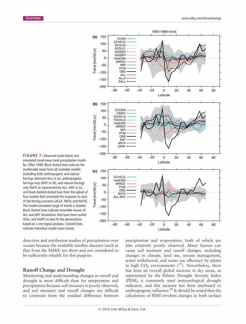
Another expected aspect of simulated precipi-tation change is a latitudinal redistribution of pre-cipitation including increasing precipitation at highlatitudes and decreasing precipitation at subtropicallatitudes, and potentially changes in the distribution of

precipitation within the tropics by shifting the positionof the Intertropical Convergence Zone. Comparisonsbetween observed and modeled trends in land precip-itation over two periods during the 20th century areshown in Figure 7. A comparison of observed trendsaveraged over latitudinal bands with those simulatedby 14 climate models forced by the combined effects ofanthropogenic and natural external forcing, and by 4climate models forced by natural forcing alone, showsthat anthropogenic forcing has had a detectable influ-ence on observed changes in average precipitation.55

While these changes cannot be explained by internalclimate variability or natural forcing, the magnitude ofchange in the observations is greater than simulated.

The influence of anthropogenic greenhouse gasesand sulfate aerosols on changes in precipitation overhigh-latitude land areas north of 55◦N has alsobeen detected.56 Detection is possible here, despitelimited data coverage, in part because the responseto forcing is relatively strong in the region, andbecause internal variability is low, as is expected indry regions. Consistent with this argument, there hasbeen some consistency in northern Europe winterprecipitation between that from observations and thatfrom simulations conducted by four different regionalclimate models.38 Generally, however, detection andattribution of regional precipitation changes remainsdifficult because of low signal-to-noise ratios and poorobservational coverage. To date there have been no



FIGURE 7 | Observed (solid black) andsimulated zonal-mean land precipitation trendsfor 1950–1999. Black dotted lines indicate themultimodel mean from all available models(including both anthropogenic and naturalforcings (denoted ALL) in (a), anthropogenicforcings only (ANT) in (b), and natural forcingsonly (NAT) as represented by ALL–ANT in (c),and black dashed-dotted lines from the subset offour models that simulated the response to eachof the forcing scenarios (ALL4, ANT4, and NAT4).The model-simulated range of trends is shaded.Black dashed lines indicate ensemble means ofALL and ANT simulations that have been scaled(SALL and SANT) to best fit the observationsbased on a one-signal analysis. Colored linesindicate individual model mean trends.

−200

SALLALL4ALL

OBSPCMMRI

MIROCHadCM3GISSERGISSEHGFDL21GFDL20

SANTANT4ANTOBSPCMMPI

MIROC

ALL-ANTNAT4OBSPCM

MIROCHadCM3ECHO-G

HadCM3FGOALSECHO-G

CSIROCCCMA

ECHO-GCCSM

−80 −60 −40 −20 0 20 40 60 80Latitude

−80 −60 −40 −20 0 20 40 60 80Latitude

−80 −60 −40 −20 0 20 40 60 80Latitude

1950-1999 trend

Tre

nd [m

m/5

0-yr

]

−150

−100

−50

0

50

100

150(a)

−200

Tre

nd [m

m/5

0-yr

]

−150

−100

−50

0

50

100

150(b)

−200

Tre

nd [m

m/5

0-yr

]

−150

−100

−50

0

50

100

150(c)

detection and attribution studies of precipitation overoceans because the available satellite datasets (such asthat from the SSM/I) are short and not considered tobe sufficiently reliable for this purpose.

Runoff Change and DroughtMonitoring and understanding changes in runoff anddrought is more difficult than for temperature andprecipitation because soil moisture is poorly observed,and soil moisture and runoff changes are difficultto constrain from the residual difference between

precipitation and evaporation, both of which arealso relatively poorly observed. Many factors cancause soil moisture and runoff changes, includingchanges in climate, land use, stream management,water withdrawal, and water use efficiency by plantsin high CO2 environments (57). Nevertheless, therehas been an overall global increase in dry areas, asrepresented by the Palmer Drought Severity Index(PDSI), a commonly used meteorological droughtindicator, and this increase has been attributed toanthropogenic influence.58 It should be noted that thecalculation of PDSI involves changes in both surface



temperature and precipitation but is dominated bychanges in temperature, and therefore, detection inPDSI is largely associated with increased temperaturesrather than changes in precipitation.

Despite more intensive human water consump-tion, continental runoff has increased through the 20thcentury. Gedney et al.,57 using a surface exchangescheme driven by observations and climate modelsimulations, detect anthropogenic influence on globalrunoff. They attribute the observed increase in runoffto a suppression of plant transpiration resulting fromCO2-induced stomatal closure57 although it has beenargued that data limitations call the conclusions ofthis study into question.57,59

In climates where seasonal snow storage andmelting plays a significant role in annual runoff, thehydrologic regime changes with temperature. In awarmer world, less winter precipitation falls as snowand the melting of winter snow occurs earlier in spring,resulting in a shift in peak river runoff to winter andearly spring. This has been observed in the westernUS60 and in Canada.61 The observed trends towardearlier ‘center’ timing of snowmelt-driven streamflowsin the western US since 1950 are detectably differentfrom natural variability.62 A recent detection studyof change in the hydrological cycle of the westernUS attributes up to 60% of observed climate relatedtrends in river flow, winter air temperature, and snowpack over the 1950–1999 period in the region tohuman influence.63

CryosphereAmong the varios parameters characterizing changesin snow cover, snow cover duration has the strongestsensitivity to variations in climate.64 Maritimeclimates with extensive winter snowfall (e.g., thecoastal mountains of western North America) aremost sensitive and continental interior climates withrelatively cold, dry winters are least sensitive. Thelargest observed decreases in snow cover duration areconcentrated where seasonal mean air temperaturesare within 5◦C of zero, a zone which extends aroundthe midlatitudinal coastal margins of the continents.Climate model simulations of the 20th century showsnow cover changes similar to those observed.64 Therehas been a reduction in the ratio of precipitation fallingas snow in the western US that cannot be explainedby climate models including only the natural effectsof solar and volcanic forcings and which has beenattributed to anthropogenic forcings.63,65

Decreases in Arctic sea ice, shown inFigure 8, are seen in both observations and inclimate model simulations including anthropogenic

forcings,66 although few model simulations showtrends in sea ice extent of comparable magnitudeto observations.67 Human influence on Arctic sea icedecline is detectable in an optimal detection analysis68

and could have been detected as early as 1992, wellbefore the last recent dramatic sea ice retreat. In addi-tion, the anthropogenic signal is also detectable forindividual months from May to December, suggest-ing that human influence, strongest in late summer,now also extends into colder seasons.68 In contrast,Antarctic sea ice has not significantly decreased.

CIRCULATION CHANGES

Two of the major global modes of variability are theNAM and SAM. Upward trends in these modes havebeen shown to be inconsistent with simulated internalvariability (Hegerl et al.2 and references cited therein).

While the NAM trend is larger than that simu-lated in many climate model simulations,69 the trendin the SAM is consistent with simulated trends insimulations including greenhouse gas increases andstratospheric ozone depletion.70 However, model sim-ulations can show positive trends in the annular modesat the surface, but negative trends higher in the atmo-sphere, and it has been argued that anthropogeniccirculation changes are poorly characterized by trendsin the annular modes.71

Until recently, formal detection and attributionanalyses of sea level pressure (SLP) have been restrictedto individual seasons,72–74 and while these studies alldetected the influence of external forcing on SLP,none of them were able to separately detect the effectsof anthropogenic and natural influences. Recently,Gillett and Stott75 carried out a detection andattribution analysis using SLP from all four seasonsover the 60-year period 1949–2009. Observed SLP,taken from HadSLP2,76 was compared with outputfrom two ensembles of simulations of HadGEM1.77,78

The first included anthropogenic greenhouse gases,aerosols, and stratospheric ozone depletion (ANT),and the second ensemble also included volcanicaerosol and solar variability (ALL).

Figure 9 shows linear trends in zonal-meanSLP for each season over the period 1949–2009 inobservations and the ALL ensemble. As expected, thelargest trends are observed in DJF, with decreasesin SLP over the Arctic and Antarctic. However, oneaspect of the trend pattern which has not receivedmuch attention is the significant increase in SLPobserved in all latitude bands between 32.5◦N and62.5◦S.75 An increase in SLP is also simulated inall these latitude bands. The signal-to-noise ratio of



Dec

−2.4−2.1−1.8−1.5−1.2−0.9−0.6−0.3

0.30.6

−0.8

106

km2

−0.7−0.6−0.5−0.4−0.3−0.2−0.1

0.10.2

−0.8−0.7−0.6−0.5−0.4−0.3−0.2−0.1

0.10.2

1956

OBS

ANT

ALL

1962 1968 1974 1980 1986 1992 1998 2004

1956 1962 1968 1974 1980 1986 1992 1998 2004

1956 1962 1968 1974 1980 1986 1992 1998 2004

Sep

Jun

Mar

Dec

Sep

Jun

Mar

Dec

Sep

Jun

Mar

FIGURE 8 | Seasonal evolution ofobserved and simulated Arctic sea ice extent(ASIE) over 1953–2006. ASIE anomaliesrelative to the respective 1953–1982 meansfrom observations (OBS) and 20C3M modelsimulations with anthropogenic only (ANT)and natural plus anthropogenic (ALL) forcingsare plotted. Adapted from Min et al.68

these trends is generally higher than for the high-latitude trends, due to better sampling and lowerinternal variability. The other seasons generally showa similar pattern of trends to that seen in DJF, withdecreases simulated and observed in the polar regionsand increases at low latitudes, particularly, in themidlatitudes of the Southern Hemisphere.

Gillett and Stott75 applied a detection andattribution analysis using 5-year mean SLP in theseven latitude bands shown and for each of the fourseasons. They were able to detect an anthropogenicresponse independently of the natural response andwith an amplitude consistent between model andobservations. These results suggest that while modelsmay fail to reproduce SLP trends in DJF over thehigh northern latitudes,70,73 a more complete analysisconsidering all regions and seasons does not find asignificant bias in the amplitude of the simulated SLPresponse to external forcing.

Some evidence has been found for changesin atmospheric storminess. The trend pattern inatmospheric storminess as inferred from geostrophicwind energy and ocean wave heights has been foundto contain a detectable response to anthropogenic andnatural forcings with the effect of external forcingsbeing strongest in the winter hemisphere.74

OCEANIC CHANGESIt has been estimated that over 80% of the excess heatbuilt up in the climate system by anthropogenic forcinghas accumulated in the global oceans79 and thereforeit is important to understand oceanic variability andchanges since uptake of heat by the ocean actsto mitigate transient surface temperature rise. TheIPCC AR4 report concluded that the warming ofthe upper ocean during the latter half of the 20thcentury was likely due to anthropogenic forcing.



−75

−2 −1 0 1

SLP trend (hPa)

Latit

ude

−50

−25

0

25

50

75

DJFMAMJJASON

FIGURE 9 | Trends in seasonal mean sea level pressure in seven 25◦-latitude bands between 87.5◦S and 87.5◦N calculated from 5-year meansover the period December 1949–November 2009. Solid lines show observed trends from HadSLP2, and dashed lines show ensemble mean trends inthe ALL simulations of HadGEM1. Gray bands represent the approximate 5–95% range of simulated SLP trends in a control simulation of HadGEM1.MAM, JJA and SON trends are offset from DJF trends by 2, 4 and 6 hPa, respectively. Vertical dotted lines indicate zero trend for each season.Adapted from Gillett and Stott.75

This conclusion was based largely on the studiesof Barnett et al.80 and Pierce et al.81 who extendedprevious detection and attribution analyses of oceanheat content changes,82,83 to a basin by basin analysisof the temporal evolution of temperature changesin the upper 700 m of the ocean and who detecteda human-induced warming of the world’s oceanswith a complex vertical and geographical structure.However, while there was very strong statisticalevidence that the warming could not be explainedby internal variability as estimated by two differentclimate models, there were discrepancies betweenobserved and modeled estimates of global ocean heatcontent variability. A large part of this discrepancyhas now been seen to be associated with instrumentalerrors,84 and there is much improved agreement whenthese bias corrections are included in observationaldatasets.85

However, the subsurface ocean has been sparselyobserved in many regions, and sampling errors remainan issue when comparing observed and modeledtimeseries of ocean properties, with the choice ofinfilling method being potentially important in poorlysampled regions.86,87 A novel process-based techniquefor comparing models and observations has beenproposed,88,89 which separates ocean warming into acomponent largely associated with changes in air–seaheat flux (the temperature above the 14C isotherm)and a component largely associated with advectiveredistribution of heat (the depth of the 14C isotherm).This provides a clearer picture of the drivers of oceanic

temperature changes. Figure 10, from Palmer et al.,90

shows that the HadCM3 climate model captures inremarkable detail the temporal evolution of oceantemperatures in the World’s ocean basins over thelast five decades. By comparing space time patternsaveraged over nonoverlapping 2-year periods for fivedifferent ocean basins, Palmer et al.90 detected theeffects of both anthropogenic and volcanic influencessimultaneously in the observed record. This providedan advance on previous studies by attributing theshort-term cooling episodes to volcanic eruptions andthe multidecadal warming to anthropogenic forcing.

The other major property of ocean water massesis their salinity. Changes in salinity are of interestbecause they integrate changes in precipitation andevaporation at the surface and could therefore helpbetter understand changes in the hydrological cycleover the sparsely observed ocean. It has been suggestedthat freshening at high latitudes is consistent withobserved increases in precipitation at high latitudes91

although climate model studies suggest that Atlanticfreshening could be associated with changes innorthward advection associated with variability ofthe meridional overturning circulation.92 An optimaldetection analysis of Atlantic salinity changes by Stottet al.93 detected a human influence on the observedincreases in salinity at low latitudes but found thathigh-latitude changes, including a recent reversal ofthe freshening observed previously, are consistent withinternal variability.



−0.31950 1960 1970 1980 1990 2000

Year

1950 1960 1970 1980 1990 2000

Year

1950 1960 1970 1980 1990 2000

Year

1950 1960 1970 1980 1990 2000

Year

Tem

pera

ture

ano

mal

y (°

C)

−0.2

−0.1

0.0

0.1

Agung

Global ocean

Chichon Pinatubo Agung

Atlantic ocean

Chichon Pinatubo

Agung

Pacific ocean

Chichon Pinatubo Agung

Indian ocean

Chichon Pinatubo

0.2

0.3

−0.3

Tem

pera

ture

ano

mal

y (°

C)

−0.2

−0.1

0.0

0.1

0.2

0.3

−0.3

Tem

pera

ture

ano

mal

y (°

C)

−0.2

−0.1

0.0

0.1

0.2

0.3

−0.3

Tem

pera

ture

ano

mal

y (°

C)

−0.2

−0.1

0.0

0.1

0.2

0.3

(a) (b)

(c) (d)

FIGURE 10 | Time series of global ocean temperature above the 14◦C isotherm relative to 1950–1999 average for (a) global ocean, (b) AtlanticOcean, (c) Pacific Ocean, and (d) Indian Ocean. Shown are the observations (black); the ensemble average of four HadCM3 simulations including bothanthropogenic and natural forcings (red) and ensemble standard deviation (orange shading); and the ensemble average of four HadCM3 simulationsincluding only natural forcings (blue) and ensemble standard deviation (light blue shading). The model data have been regridded and subsampled tomatch the observational coverage. The vertical lines show the approximate timing of the major volcanic eruptions. Adapted from Palmer et al.90

A major research topic remains an improvedunderstanding of the rate of global sea level rise and itscontributions from thermal expansion and melting ofland ice, and a reduction in uncertainty in predictionsof the geographical patterns of sea level rise. Futureprogress in attributing ocean changes could bemade by considering water masses properties.94,95

By considering temperature and salinity changes ondensity surfaces, it could be possible to better quantifythe effects of anthropogenic and natural forcings onocean heat content and better quantify the extent towhich external forcings have altered the hydrologicalcycle over the oceans.96,97

EXTREMES

Many analyses of changes in extremes have focusedon globally collected indices of climate extremeswhich summarize overall characteristics of extremes

and are derived from high resolution data (see,e.g., Alexander et al.98). Observed changes in suchindices are broadly consistent with changes expectedwith global warming; only with the inclusion ofanthropogenic forcing can models reproduce theobserved changes in frost days, growing season length,the number of warm nights in a year, and a heat waveintensity index.99 An observed precipitation intensityindex also appears to track simulated changes.100

Rather than analyze indices, Christidis et al.101

analyzed the daily temperature dataset of Caesaret al.102 and found a significant human influence onthe observed warming of the warmest night of theyear as well as on warming of the coldest daysand nights of each year. However, they did notdetect a significant change in the temperature of thehottest day of the year. Extremes of daily maximumtemperatures show distinct regional patterns. Recentresearch suggests that some of these regional trendscould be related to regional processes and forcings.



01 4 10 20

Number of occurrences per thousand years

Est

imat

ed li

kelih

ood

(nor

mal

ized

)

0.2

0.4

0.6

0.8

FIGURE 11 | Change in probability of mean European summertemperatures exceeding the 1.6 K threshold showing histograms offrequency of such events under late 20th century conditions in theabsence of anthropogenic climate change (green line) and withanthropogenic climate change (red line). From Stott et al.105 Thedistributions represent the uncertainty in this calculation’s estimate ofthe frequencies of such events in the two cases.

For example, Portmann et al.103 demonstrated that therate of increase in the number of hot days per year inlate spring in the Southeastern US over recent decadesis significantly inversely proportional to climatologicalprecipitation. They speculate that changes in biogenicaerosols resulting from land use changes could beresponsible.

In addition to analyzing trends in extremes, anew framework has been developed for attributingindividual extreme events. In such a framework, aselucidated by Allen,104 the change in the probabilityof an extreme event under current conditions iscalculated and compared with the probability of theevent if the effects of particular external forcings,such as due to human influence, had been absent. Insuch a way Stott et al.105 showed that the probabilityof seasonal mean temperatures as warm as thoseobserved in Europe in 2003 had very likely at leastdoubled as a result of human influence (see Figure 11).The same general approach could, in theory, beapplied to other extreme weather events such asfloods or droughts, in order to determine whetherthe probability of a particular event has changed asa result of a chosen set of climate forcing factors,although in practice this will require models capableof capturing the relevant processes.

Attributing causes to changes in the frequencyand intensity of hurricanes has remained verycontroversial. Two studies,106,107 have shown thathuman-caused changes in greenhouse gases are themain driver of the observed 20th-century increasesin sea surface temperatures in the main hurricaneformation regions of the Atlantic and the Pacific.

However, the importance of the anthropogenicincrease in sea surface temperature in the cyclogensisregion for past and future changes in hurricane activityis still poorly understood.108 The limitations of theobserved database and of current climate modelsin resolving processes relevant for hurricanes makeprogress in this field difficult at present.

In conclusion, while there has been progresssince AR4, there are still many gaps in ourunderstanding of changes in extremes and in ourability to attribute observed changes to particularcauses. Changes in temperature extremes have provento be more interesting and difficult than an assumptionof a shift of the distribution would lead to expect,particularly so for daily maxima.103 While attributionof change in precipitation extremes is made difficultby the lack of tools for reliable comparison of modelswith observations, perfect model studies indicate thatchanges in precipitation extremes should be detectableat least on large scales.109

CONCLUSION

The wealth of attribution studies reviewed in thisarticle shows that there is an increasingly remotepossibility that climate change is dominated bynatural rather than anthropogenic factors. Progresssince the AR4 has shown that discernible humaninfluence extends to reductions in Arctic sea iceand changes in the hydrological cycle associatedwith increasing atmospheric moisture content, globaland regional patterns of precipitation changes, andincreases in ocean salinity in Atlantic low latitudes.In addition, changes in Antarctic temperatures (theone continent on which an attribution study was notavailable at the time of AR4) have been attributedto human influence and there is increasing evidencethat human influence on temperature is becomingsignificant below continental scales, as would beexpected from the large-scale coherence of surfacetemperature. We have discussed in this review howattributed changes in atmospheric moisture content49

and precipitation patterns55 are consistent withtheoretical expectations.45,46

At times, attribution studies can highlight differ-ences between models and observations that challengeour understanding and require further investigation.Major challenges still remain in obtaining robustattribution results at the regional scales needed forevaluation of impacts. Climate models often lackthe processes needed to realistically simulate regionaldetails. In addition, observed changes in non-climatequantities could be the result of additional influences



besides climate, thus complicating attribution stud-ies. Extremes pose a particular challenge, since rareevents are, by definition, poorly sampled in the histor-ical record, and many challenges remain for robustlyattributing regional changes in extreme events such asdroughts, floods, and hurricanes.

Nevertheless, successful adaptation would bene-fit from improved information about societal vulnera-bility in a changing climate.110 We have discussed herehow the changed likelihood of a particular weatherevent can be attributed to human influence, and inprinciple, such a concept could be applied to anyextreme weather event and its associated impacts.Models of higher resolution will likely be required toresolve processes responsible for events such as floods.Atmosphere only models, constrained by prescribedsea surface temperatures, can be used to address thecauses of specific events, although atmosphere–oceancoupling and the causes of the sea surface conditionsalso need to be considered.

Above all, understanding observed changes isan essential prerequisite for successful forecastingof future changes. Further research on the use of

observational constraints has the potential to reducethe large spread from modeling uncertainty, some ofwhich could be slow to reduce purely based on theimprovement of model formulation. Thus this suggeststwo key benefits from attribution studies for improv-ing climate model predictions. First, by finding robustrelationships between observed quantities and predic-tor variables, attribution studies can be used to obtainobservationally constrained estimates of uncertaintiesin future changes. This approach has been applied toglobal mean surface temperature but further researchis needed to extend this approach to regional scaletemperatures and other variables. Second, attributionstudies, by identifying model data differences thatare outside the range expected from natural internalvariability, have the potential to highlight inadequa-cies in model forcing or formulation or problems withobservational datasets. In some instances, better repre-sentation of regional changes in models might requireinclusion of hitherto neglected forcings or better rep-resentation of crucial processes. In others, efforts maybe needed to better account for errors and systematicbiases in observational data.

ACKNOWLEDGEMENTS

P.A.S. was supported by the Joint DECC and Defra Integrated Climate Programme—DECC/Defra (GA01101).The authors acknowledge the support of the International Detection and Attribution group by the US departmentof Energy’s Office of Science, Office of Biological and Environmental Research and the US National Oceanicand Atmospheric Administration’s Climate Program Office.DAS was funded by Microsoft Research.

REFERENCES

1. Solomon S, Qin D, Manning M, Chen Z, MarquisM, et al. Climate Change 2007: The Physical ScienceBasis. Contribution of Working Group I to the FourthAssessment Report of the Intergovernmental Panel onClimate Change. Cambridge: Cambridge UniversityPress; 2007.

2. Hegerl GC, Zwiers FW, Braconnot P, Gillett NP, LuoY, et al. In: Solomon S, Qin D, Manning M, Chen Z,Marquis M, et al., eds. Understanding and AttributingClimate Change Climate Change 2007: The PhysicalScience Basis. Contribution of Working Group I tothe Fourth Assessment Report of the Intergovernmen-tal Panel on Climate Change. Cambridge: CambridgeUniversity Press; 2007.

3. Easterling DR, Wehner MF. Is the climate warm-ing or cooling? Geophys Res Lett 2009, 36:L08706.DOI:10.1029/2009GL037810.

4. Knight J, Kennedy JJ, Folland C, Harris G, Jones GS,et al. Do global trends over the last decade falsifyclimate predictions? BAMS. In BAMS State of theClimate 2008. July, 2009.

5. Zorita E, Stocker TF, von Storch H. How unusual isthe recent series of warm years? Geophys Res Lett2008, 35:L24706. DOI:10.1029/2008GL036228.

6. Trenberth KE. An imperative for climate changeplanning: tracking Earth’s global energy. Curr OpinEnviron Sustainability 2009, 1:19–27.

7. Brohan P, Kennedy JJ, Harris I, Tett SFB, JonesPD. Uncertainty estimates in regional and globalobserved temperature changes: a new datasetfrom 1850. J Geophys Res 2006, 111:D12106.DOI:10.1029/2005JD006548.

8. Min SK, Hense A, Paeth H, Kwon WT. A Bayesiandecision method for climate change signal analysis.Meterol Z 2004, 13:421–436.



9. Schnurr R, Hasselman K. Optimal filtering forBayesian detection and attribution of climate change.Clim Dyn 2005, 24:45–55.

10. Stott PA, Tett SFB. Scale-dependent detection of cli-mate change. J Clim 1998, 11:3282–3294.

11. Wu Q, Karoly DJ. Implications of changes in theatmospheric circulation on the detection of regionalsurface air temperature trends. Geophys Res Lett2007, 34:L08703. DOI:10.1029/2006GL028502.

12. Shindell D, Faluvegi G. Climate response to regionalradiative forcing during the twentieth century. NatGeosci 2009, 2:294–300.

13. Meehl GA, Washington WM, Ammann CM,Arblaster JM, Wigley TML, et al. Combinations ofnatural and anthropogenic forcings in 20th centuryclimate. J Clim 2004, 17:3721–3727.

14. Gillett NP, Wehner MF, Tett SFB, Weaver AJ. Testingthe linearity of the response to combined greenhousegas Geophys Res Lett 2004, 31:L14201.

15. Knutson TR, Delworth TL, Dixon KW, Lu J, et al.Assessment of twentieth-century regional surface tem-perature trends using the GFDL CM2 coupled models.J Clim 2006, 19:1624–1651.

16. Sexton DMH, Grubb H, Shine KP, Folland CK.Design and analysis of climate model experimentsfor the efficient estimation of anthropogenic signals.J Clim 2003, 16:1320–1336.

17. Meehl GA, Washington WM, Wigley TML, ArblasterJM, Dai A. Solar and greenhouse gas forcing andclimate response in the 20th century. J Clim 2003,16:426–444.

18. IDAG. Detecting and attributing external influ-ences on the climate system: a review ofrecent advances. J Clim 2005, 18:1291–1314. DOI:10.1175/JCLI3329.

19. Allen MR, Tett SFB. Checking for model consis-tency in optimal finger printing. Clim Dyn 1999,15:419–434.

20. Parker DE, Alexander LV, Kennedy J. Global andregional climate in 2003. Weather 2004, 59:145–152.

21. Stott PA, Mitchell JFB, Allen MR, Delworth TL,Gregory JM, et al. Observational constraints on pastattributable warming and predictions of future globalwarming. J Clim 2006, 19:3055–3069.

22. Huntingford C, Stott PA, Allen MR, Lambert FH.Incorporating model uncertainty into attribution ofobserved temperature change. Geophys Res Lett2006, 33:L05710. DOI:10.1029/2005GL024831.

23. Christidis N, Stott PA, Zwiers FW, Shiogama H,Nozawa T. Probalistic estimates of recent changes intemperature: a multi-scale attribution analysis. ClimDyn 2009. DOI:10.1007/s00382-009-0615-7.

24. Allen MR, Stott PA, Mitchell JFB, Schnur R, DelworthT. Quantifying the uncertainty in forecasts of anthro-pogenic climate change. Nature 2000, 407:617–620.

25. Frame DJ, Stone DA, Stott PA, Allen MR. Alternativeto stabilization scenarios. Geophys Res Lett 2006,33:L14707. DOI:10.1029/2006GL025801.

26. Stott PA, Huntingford C, Jones CD, KettleboroughJA. Observed climate change constrains the likeli-hood of extreme future global warming. Tellus A2008, 60B:76–81.

27. Brasseur GP, Roeckner E. Impact of improvedair quality on the future evolution of cli-mate. Geophys Res Lett 2005, 32:L23704.DOI:10.1029/2005GL023902.

28. Stott PA. Attribution of regional-scale tem-perature changes to anthropogenic and natu-ral causes. Geophys Res Lett 2003, 30:1724.DOI:10.1029/2003GL01732.

29. Karoly DJ, Braganza K, Stott PA, Arblaster JM, MeehlGA. Detection of a human influence on North Americaclimate. Science 2003, 302:1200–1203.

30. Zwiers fW, Zhang X. Towards regional scale climatechange detection. J Clim 2003, 16:793–797.

31. Gillett NP, Stone DA, Stott PA, Nozawa T, KarpechkoAY, et al. Attribution of polar warming to humaninfluence. Nat Geosci 2008, 1:750–754.

32. Min S-K, Hense A. A Bayesian assessment of climatechange using multimodel ensembles. Part II: regionaland seasonal mean surface temperatures. J Clim 2007,20:2769–2790.

33. Jones GS, Stott PA, Christidis N. Human contribu-tion to rapidly increasing frequency of very warmNorthern Hemisphere summers. J Geophys Res 2008,113:D02109. DOI:10.1029/2007JD008914.

34. Giorgi F. Variability and trends of sub-continentalscale surface climate in the 20th century. Part I: obser-vations. Clim Dyn 18:675–691.

35. Zhang X, Zwiers FW, Stott PA. Multimodel multisig-nal climate change detection at regional scale. J Clim2006, 19:4294–4307.

36. Gillett NP, Weaver AJ, Zwiers FW, Flannigan MD.Detecting the effect of climate change on Canadianforest fires. Geophys Res Lett 2004, 31:L18211.DOI:10.1029/2004GL020876.

37. Thompson DWJ, Wallace JM, Hegerl GC. Annularmodes in the extratropical circulation. Part II trends.J Clim 2000, 13:1018–1036.

38. Bhend J, von Storch H. Consistency of observedwinter precipitation trends in northern Europe withregional climate change projections. Clim Dyn 2008,31:17–28.

39. Bonfils C, Santer BD, Pierce DW, Hidalgo HG,Bala G, et al. Detection and attribution of temper-ature changes in the mountainous western UnitedStates. J Clim 2008, 21:6404–6424.



40. Lobell DB, Bonfils C. The effect of irrigation onregional temperatures: a spatial and temporal analy-sis of trends in California, 1934–2002. J Clim 2008,21:2063–2071.

41. Narisma GT, Pitman AJ. The impact of 200 yearsof land cover change on the Australian near-surfaceclimate. J Hydromet 2003, 4:424–436.

42. Feddema J. A comparison of a GCM response to his-torical anthropogenic land cover change and modelsensitivity to uncertainty in present-day land coverrepresentations. Clim Dyn 2005, 25:581–609.

43. Karoly DJ, Stott PA. Anthropogenic warming ofcentral England temperature. Atmos Sci Lett 2006,7:81–85. DOI:10.1002/asl.136.

44. Dean SM, Stott PA. The effect of local circula-tion variability on the detection and attributionof New Zealand temperature trends. J Clim 2009,22:6217–6229.

45. Allen MR, Ingram WJ. Constrains on future changesin climate and the hydrologic cycle. Nature 2002,419:224–232.

46. Held IM, Soden BJ. Robust responses of thehydrological cycle to global warming. J Clim 2006,19:5686–5699.

47. Willett KM, Gillett NP, Jones PD, Thorne PW.Attribution of observed surface humidity changesto human influence. Nature 2007, 449:710–713.DOI:10.1038/nature06207.

48. Willett KM, Jones PD, Gillett NP, Thorne PW.Recent changes in surface humidity: development ofthe HadCRUH Dataset, J Clim 2008, 21:5364–5383.DOI:10.1175/2008jcli2274.1.

49. Santer BD, Mears C, Wentz FJ, Taylor KE, GlecklerPJ, et al. Identification of human-induced changes inatmospheric moisture content. Proc Natl Acad SciU S A 2007, 104:15248–15253. DOI:10.1073/pnas.0702872104.

50. Mitchell JFB, Wilson CA, Cunningham WM. On CO2

climate sensitivity and model dependence of results.Q J R Meterol Soc 1987, 113:293–322.

51. Wentz FJ, Ricciardulli L, Hilburn K, Mears C, 2007.How much more rain will global warming bring?Science 317:233–235. DOI:10.1126/science.ll40746.

52. Liepert BG, Previdi M. Do models and observationsdisagree on the rainfall response to global warming?J Clim 2009, 22:3156–3166.

53. Lambert FH, Stott PA, Allen MR, Palmer MA. Detec-tion and attribution of changes in 20th century landprecipitation. Geophys Res Lett 2004, 31:L10203.DOI:10.1029/2004GL019545.

54. Lambert FH, Allen MR. Are changes in global precipi-tation constrained by the tropospheric energy budget?J Clim 2009, 23:499–517.

55. Zhang X, Zwiers FW, Hegerl GC, Lambert FH,Gillett NP, et al. Detection of human influence on

twentieth-century precipitation trends. Nature 2007,448:461–466. DOI:10.1038/nature06025.

56. Min S-K, Zhang X, Zwiers FW. Human-inducedArctic moistening. Science 2008, 320:518–520.DOI:10.1126/science.115346.

57. Gedney N, Cox PM, Betts R, Boucher O, Hunt-ingford C, et al. Detection of a direct carbon dioxideeffect in continental river runoff records. Nature 2006,439:835–838. DOI:10.1038/nature04504.

58. Burke E, Brown SJ, Christidis N, et al. Modelling therecent evolution of global drought and projections forthe 21st century with Hadley Centre climate model.J Hydrometeorol 7:1113–1125.

59. Peel MC, McMahon TA. Continental runoff: aquality-controlled global runoff data set. Nature2006, 444. DOI:10.1038/nature05480.

60. Regonda SK, Rajagopalan B, Clark M, Pitlick J. Sea-sonal cycle shifts in hydroclimatology over the westernUnited States. J Clim 2005, 18:372–384.

61. Zhang X, Harvey KD, Hogg WD, Yuzyk TR. Trendsin Canadian streamflow. Water Resources Res 2001,37:987–998.

62. Hidalgo HG, Das T, Dettinger MD, Cayan DR,Pierce DW, et al. Detection and attribution of stream-flow timing changes to climate change in westernUnited States. J Clim 2009, 22:3838–3855.

63. Barnett TP, Pierce DW, Hidalgo HG, Bonfils C, SanterBD, et al. Human-induced changes in the hydrol-ogy of the Western United States. Science 2008,319:1080–1083. DOI:10.1126/science.1152538.

64. Brown R, Mote PW. The response of Northern Hemi-sphere snow cover to a changing climate. J Clim 2009,22:2124–2145.

65. Pierce DW, Barnett TP, Hidalgo HG, Das T, Bonfils C,et al. Attribution of declining western US snowpacksto human effects. J Clim 2008, 21:6425–6444.

66. Gregory JM, Stott PA, Cresswell DJ, Rayner N, Gor-don C, et al. Recent and future changes in Arctic seaice simulated by the HadCM3 AOGCM. Geophys ResLett 2002, 29:2175. DOI:10.1029/2001GL014575.

67. Stroeve J, Holland MM, Meier W, Scambos T,Serreze M. Arctic sea ice decline: faster thanforecast. Geophys Res Lett 2007, 34:L09501.DOI:10.1029/2007GL029703.

68. Min S-K, Zhang X, Zwiers FW, Agnew T. Humaninfluence on Arctic sea ice detectable from early1990s onwards. Geophys Res Lett 2008, 35:L21701.DOI:10.1029/2008GL035725.

69. Gillett NP. Northern Hemisphere circulation. Nature2005, 437:496.

70. Miller RL, Schmidt GA, Shindell DT, 2006. Forcedvariations in the annular modes in the 20th centuryIPCC AR4 simulations. J Geophys Res 111, D18101.DOI:10.1029/2005JD006323.



71. Woollings T. The vertical structure of anthro-pogenic zonal-mean atmospheric circulationchange. Geophys Res Lett 2008, 35:L19702.DOI:10.1029/2008GL034883.

72. Gillett NP, Zwiers FW, Weaver AJ, Stott PA. Detec-tion of human influence on sea level pressure. Nature2003, 422:292–294.

73. Gillett NP, Allan RJ, Ansell TJ. Detection of exter-nal influence on sea level pressure with a multi-model ensemble. Geophys Res Lett 2005, 32:L19714.DOI:10.1029/2005GL023640.

74. Wang XL, Swail VR, Zwiers FW, Zhang X, Feng Y.Detection of external influence on trends of atmo-spheric storminess and northern oceans wave heights.Clim Dyn 2008, 32:189–203. DOI:10.1007/s00382-008-0442-2.

75. Gillett NP, Stott PA. Attribution of anthropogenicinfluence on seasonal sea level pressure. Geophys ResLett 2009 36:L23709. DOI:10.1029/2009GL041269.

76. Allan RJ, Ansell TJ. A new globally-complete monthlyhistorical gridded mean sea level pressure data set(HadSLP2): 1850-2004. J Clim 2006, 19:5816–5842.

77. Johns TC, Durman CF, Banks HT, Roberts MJ,McLaren AJ. The new Hadley Centre climate modelHadGEM1: evaluation of coupled simulations. J Clim2006, 19:1327–1353.

78. Stott PA, Jones GS, Thorne PW, Lowe JA, Durman C.Transient climate simulations with the HadGEM1climate model: causes of past warming and futureclimate change. J Clim 2006, 19:2763–2782.

79. Levitus S, Antonov J, Boyer T. Warming of theWorld ocean, 1955-2003. Geophys Res Lett 2005,32:L02604. DOI:10.1029/2004GL021592.

80. Barnett TP, Pierce DW, AchutaRao KM, Gleckler PJ,Santer BD, et al. Penetration of a warming signal inthe world’s oceans: human impacts. Science 2005,309:284–287.

81. Pierce DW, Barnett TP, AchutaRao KM, Gleckler PJ,Gregory JM, et al. Anthropogenic warming of theoceans: observations and model results. J Clim 2006,19:1873–1900.

82. Barnett TP, Pierce DW, Schnur R. Detection of anthro-pogenic climate change in the world’s oceans. Science2001, 292:270–274.

83. Reichert BK, Schnur R, Bengtsson L. Global oceanwarming tied to anthropogenic forcing. Geophys ResLett 2002, 29. DOI:10.1029/2001GL013954.

84. Wijffels SE, Willis J, Domingues CM, Barker P, WhiteNJ, et al. Changing expendable bathythermographfall rates and their impact on estimates of ther-mosteric sea level rise. J Clim 2008, 21:5657–5672.DOI:10.1175/2008JCLI2290.1.

85. Domingues CM, Church JA, White NJ, Gleckler PJ,Wijffels SE, et al. Improved estimates of upper-ocean

warming and multi-decadal sea-level rise. Nature2008, 453:1090–1093.

86. Gregory JM, Banks HT, Stott PA, Lowe JA, PalmerMD. Simulated and observed decadal variabilityin ocean heat content Geophys Res Lett, 2004,31:L15312. DOI:10.1029/2004GL020258.

87. AchutaRao KM, Ishii M, Santer BD, Gleckler PJ,Taylor KE, et al. Simulated and observed variabilityin ocean temperature and heat content. Proc NatlAcad Sci USA 2007, 104:10768–10773.

88. Palmer MD, Haines K, Ansell TJ, Tett SFB. Isolatingthe signal of ocean global warming. Geophys Res Lett2007, 34:L23610. DOI:10.1029/2007GL031712.

89. Palmer MD, Haines K. Estimating oceanic heatcontent change using isotherms. J Clim 2009,22:4953–4969.

90. Palmer MD, Good S, Haines K, Rayner N,Stott PA. Geophys Res Lett 2009, 36:L20709.DOI:10.1029/2009GL039491.

91. Bindoff NL, Jurgen W, Vincenzo A, Anny C,Jonathan M, et al. In: Solomon S, Qin D, ManningM, Chen Z, Marquis M, et al., eds. Unnikrish-nan Observations: Oceanic Climate Change and SeaLevel. Climate Change 2007: The Physical ScienceBasis. Contribution of Working Group I to the FourthAssessment Report of the Intergovernmental Panel onClimate Change. Cambridge: Cambridge UniversityPress; 2007.

92. Pardaens A, Vellinga M, Wu P, Ingleby B. Large-scale Atlantic salinity changes over the last half-century: a model-observation comparison. J Clim2008, 21:1698–1720.

93. Stott PA, Sutton RT, Smith DM. Detection and attri-bution of Atlantic salinity changes. Geophys Res Lett2008, 35:L21702. DOI:10.1029/2008GL035874.

94. Banks HT, Wood RA, Gregory JM, Johns TC, JonesGS. Are observed decadal changes in intermediatewater masses a signature of anthropogenic climatechange? Geophys Res Lett 2000, 27:2961–2964.

95. Stark S, Wood RA, Banks HT. Reevaluating the causesof observed changes in Indian Ocean water masses.J Clim 2006, 19:4075–4086.

96. Hegerl GC, Karl TR, Allen M, Bindoff NL, GillettN. et al. Climate change detection and attribution:beyond mean temperature signals. J Clim, 2006,19:5058–5077.

97. Helm KP, Bindoff NL, Church JA. Globalhydrological-cycle changes inferred from observedocean salinity. Geophys Res Lett 2009. In Press.

98. Alexander LV, Zhang X, Peterson TC, Cae-sar J, Gleason B, et al. Global observed changesin daily climate extremes of temperature andprecipitation. J Geophys Res 2006, 111:D05109.DOI:10.1029/2005JD006290.



99. Meehl G, Arblaster J, Tebaldi C. Contributions ofnatural and anthropogenic forcing to changes in tem-perature extremes over the United States. Geophys ResLett 2007, 34:L19709. DOI:10.1029/2007gl030948.

100. Gutowski WJ, Hegerl GC, Holland GJ, Knutson TR,Mearns LO, et al. Causes of Observed Changes inExtremes and Projections of Future Changes. InWeather and Climate Extremes in a Changing Cli-mate, US Climate Change Science Program SAP 3.3,T. Karl et al., Eds. pp. 2008, 81–116.

101. Christidis N, Stott PA, Brown S, Hegerl GC, Caesar J.Detection of changes in temperature extremes duringthe 20th century. Geophys Res Lett 2005, 32:L20716.DOI:10.1029/2005GL023885.

102. Caesar J, Alexander L, Vose R. Large-scale changesin observed daily maximum and minimum tem-peratures: creation and analysis of a new grid-ded dataset. J Geophys Res 2006, 111:D05101.DOI:10.1029/2005JD006280.

103. Portmann RW, Solomon S, Hegerl GC. Linkagesbetween climate change, extreme temperature andprecipitation across the United States. Proc Natl AcadSci U S A 2009, 106:7324–7329.

104. Allen MR. Liability for climate change. Nature 2003,421:892–892.

105. Stott PA, Stone DA, Allen MR. Human contributionto the European heatwave of 2003. Nature 2004,432:610–614.

106. Santer BD, Wigley TML, Gleckler PJ, Bonfils C,Wehner MF, et al. Forced and unforced ocean tem-perature changes in Atlantic and Pacific tropicalcyclogenesis regions. Proc Natl Acad Sci U S A 2006,103:905–913.

107. Gillett NP, Stott PA, Santer BD. Attribution of cyclo-genesis region sea surface temperature change toanthropogenic influence. Geophys Res Lett 2008,35:L09707. DOI:10.1029/GLO33670.

108. Vecchi GA, Soden BJ. Effect of remote sea surfacetemperature change on tropical cyclone potentialintensity. Nature 2007, 450:1066–1070.

109. Min S-K, Zhang X, Zwiers F, Friederichs P, Hense A.Signal detectability in extreme precipitation changesassessed from 20th century climate simulations. ClimDyn 2009, 32:95–111. DOI:10.1007/s00382-008-0376-8.

110. Stott PA, Trenberth KE. Linking extreme weatherevents to climate variability and change. EOS2009, 90:184.

FURTHER READING

Knutti R, Friedlingstein P, Gregory JM, Hegerl GC, et al. A review of uncertainties in global temperatureprojections over the twenty-first century. J Clim 2008, 21:2651–2663.


overview detection and attribution of climate change: a ... · overview detection and attribution...

Documents