over the underlying relationship between volatilities of three major u.s. market equity indexes and...

TILBURG SCHOOL OF ECONOMICS AND MANAGEMENT

Over the underlying relationship between

Volatilities of three major U.S. Market Equity

Indexes and their respective CBOE Volatility

Indexes

Supervisor:

Prof. Juan Carlos Rodríguez

Second Reader:

Prof. L.B.D Raes

Candidate:

Luca Ribichini

ANR: 914427

Dow Jones Industrial Average (DJIA)--CBOE DJIA Volatility Index (VXD)

Nasdaq 100 Index (NDX)--CBOE Nasdaq 100 Volatility Index (VXN)

Russell 2000 Index (RUT)--CBOE Russell 2000 Volatility Index (RVX)

M.SC. FINANCE THESIS

ACADEMIC YEAR

2014 - 2015

3

Abstract

In this study, I analyze the underlying relationship between the Dow Jones Industrial

Average (DJIA), Nasdaq 100 (NDX), Russell 2000 (RUT) group (henceforth: MEX) volatilities

and their respective CBOE volatility indexes group (henceforth: VOX). I examine their directional

influence by performing a set of linear regression models to assess the VOX forecast power over

its respective MEX volatility. I show that the commonly accepted view of VOX as predictor of

MEX future 22-day volatility is misleading. Indeed, this view does not reflect nor the true nor the

best relationship between these two measures. I systematically find superior R^2 and correlation

coefficients, when I start to calculate MEX volatility into the past from actual dates of VOX. Thus,

instead of predicting future volatility of its respective set of equity indexes, VOX is surprisingly

predicted in an opposite way by that set. These results are always strongly and statistically

significant. I also examine VOX and MEX future 22-day volatility empirical distributions,

comparing them against their theoretical (Normal) ones, and I find high levels of skewness and

kurtosis of empirical distributions. From an academic standpoint, it is interesting to compare these

findings to those already found about the VIX, since they would complete the analysis over the

full set of CBOE major market volatility indexes. Moreover, they would lead to an identification

of common patterns and reactions of the CBOE volatility indexes. From a market standpoint, this

work enhances the investor awareness and improve her interpretation of this relatively new set of

financial tools. Indeed, providing new empirical results and assessing recurrent patterns over each

single index, it would lead financial participants to use these volatility indexes not just as sentiment

indicators or source of hedging. It might be useful for investors who want to take a directional

view over this set of indexes, since the market (CBOE) offers options and futures over them.

5

To my grandfather

7

1. Introduction

“Volatility forecasting” is a very peculiar topic of finance literature. Indeed, volatility is a

fundamental component of each portfolio trading and hedging strategy. In finance theory, there

are two main approaches to volatility forecasting: one that uses time-series data and the other that

uses option prices (implied volatility) according to the Black-Scholes model. The popularity of the

last approach has hugely grown through the recent years and it has led to some specific volatility

indexes. The most famous one is the VIX, better known as fear index. This index, provided by the

Chicago Board Options Exchange (CBOE), is supposed to estimate over the next 30-day period

the expected volatility of S&P 500 index (SPX), by averaging the weighted prices of the S&P 500

index puts and calls over a wide range of strike prices. It is largely used by traders to have a better

understanding of investor sentiment, and thus possible reversals in the market. Its large use among

investors has induced academics to question about the VIX reliability as good predictor of S&P

500 future one-month volatility. Indeed, several studies have been conducted over the forecasting

power of the VIX and they have led to contradictory results. Poon and Granger (2003) concluded

that VIX construction is a good tool for model-based forecasting; Becker and Clemens (2007)

instead, rejected the notion that VIX contains any information for SPX volatility forecasting. Two

years later, they corrected previous conclusions (Becker and Clemens, 2009) and after having

examined the forecast performance of VIX, they concluded that VIX could not simply be viewed

as a combination of various measures in model based forecasting either. Vodenska and Chambers

(2013), in alternative, directly undertook a statistical analysis between VIX and SPX volatility

over a 20 years period, finding a reversal forecast power between these two indexes.

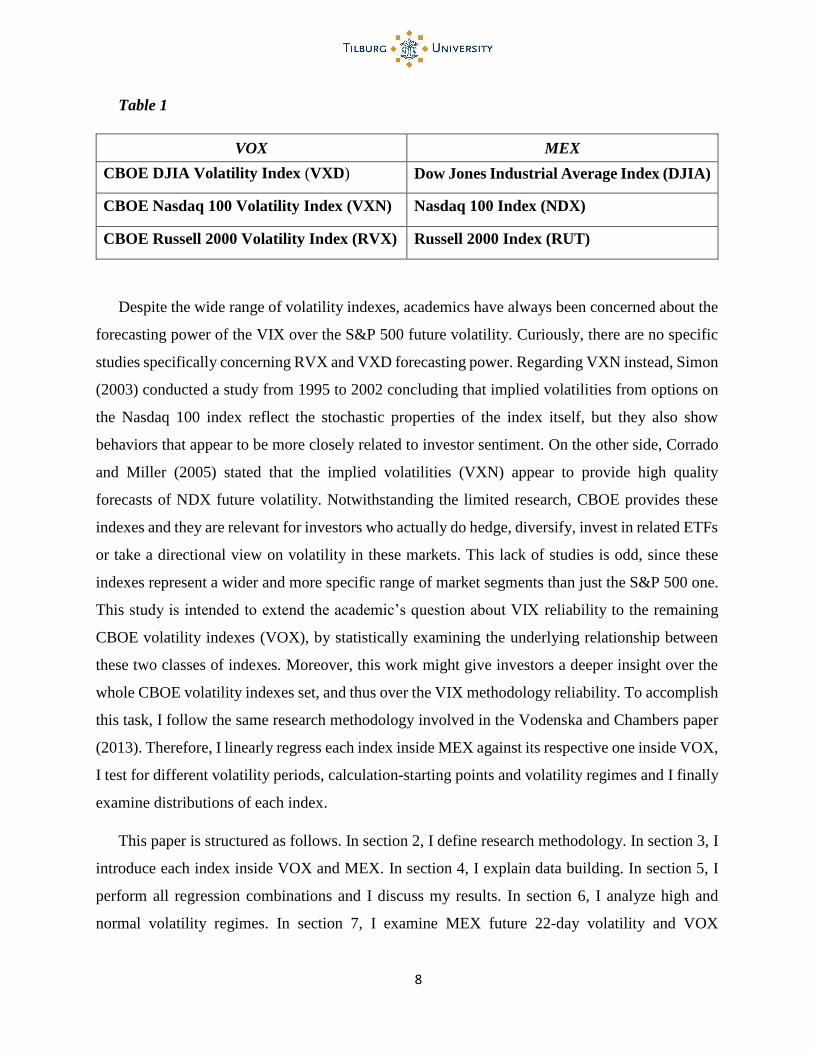
Due to the VIX great success, CBOE has extended through the years its set of volatility indexes,

using the same VIX methodology, to other U.S major market equity ones (Dow Jones Industrial

Average, Nasdaq 100, Russell 2000). This new set of volatility indexes is the one of interest of

this study. Along the paper, I refer to this set (CBOE volatility indexes group) as “VOX” and to

its respective equity set (U.S major market equity indexes group) as “MEX”. These two sets are

respectively summarized in the first and second column of Table 1, in the next page.

8

Table 1

VOX MEX

CBOE DJIA Volatility Index (VXD) Dow Jones Industrial Average Index (DJIA)

CBOE Nasdaq 100 Volatility Index (VXN) Nasdaq 100 Index (NDX)

CBOE Russell 2000 Volatility Index (RVX) Russell 2000 Index (RUT)

Despite the wide range of volatility indexes, academics have always been concerned about the

forecasting power of the VIX over the S&P 500 future volatility. Curiously, there are no specific

studies specifically concerning RVX and VXD forecasting power. Regarding VXN instead, Simon

(2003) conducted a study from 1995 to 2002 concluding that implied volatilities from options on

the Nasdaq 100 index reflect the stochastic properties of the index itself, but they also show

behaviors that appear to be more closely related to investor sentiment. On the other side, Corrado

and Miller (2005) stated that the implied volatilities (VXN) appear to provide high quality

forecasts of NDX future volatility. Notwithstanding the limited research, CBOE provides these

indexes and they are relevant for investors who actually do hedge, diversify, invest in related ETFs

or take a directional view on volatility in these markets. This lack of studies is odd, since these

indexes represent a wider and more specific range of market segments than just the S&P 500 one.

This study is intended to extend the academic’s question about VIX reliability to the remaining

CBOE volatility indexes (VOX), by statistically examining the underlying relationship between

these two classes of indexes. Moreover, this work might give investors a deeper insight over the

whole CBOE volatility indexes set, and thus over the VIX methodology reliability. To accomplish

this task, I follow the same research methodology involved in the Vodenska and Chambers paper

(2013). Therefore, I linearly regress each index inside MEX against its respective one inside VOX,

I test for different volatility periods, calculation-starting points and volatility regimes and I finally

examine distributions of each index.

This paper is structured as follows. In section 2, I define research methodology. In section 3, I

introduce each index inside VOX and MEX. In section 4, I explain data building. In section 5, I

perform all regression combinations and I discuss my results. In section 6, I analyze high and

normal volatility regimes. In section 7, I examine MEX future 22-day volatility and VOX

9

empirical and theoretical distributions. In section 8, I discuss conclusions. In section 9, I insert

references. The final part is devoted to graphs and figures I use to refer to, along the whole paper.

In Appendix, I provide graphs of the best theoretical fitting distributions of both VOX and MEX.

2. Research methodology

I follow the same research methodology of Vodenska and Chambers (2013), so I directly

undertake a statistical analysis between VOX and MEX.

I start examining the daily VOX and MEX returns for the maximum period available 1

according to each VOX (and corresponding MEX), using data from CBOE and Yahoo-Finance

databases. I run a set of linear regressions to detect whether, and to what extent, VOX predicts

MEX volatility for different periods. I first linearly regress MEX future 22-trading day (henceforth:

day) volatility2 against VOX3 to analyze the VOX forecast power over MEX future4 one-month

volatility. This first set of regression corresponds to my reference model. Secondly, I perform

regression analysis of MEX future 22-day volatility against VOX, this time including VOX past

22-day volatility as additional independent variable. I do so in order to catch any incremental

explanatory information from the simple model with just VOX as independent variable. Thirdly, I

regress different MEX volatility periods (6, 11, 33-day volatility windows) against VOX. Fourthly,

based on 22-day volatility, I shift the starting calculation point of MEX future volatility into the

past and into the future (+/- 11, 22, 33 days), in order to find the best relationship between MEX

22-day future volatility and VOX. Then, I shift again the starting point to calculate the MEX future

volatility, this time just into the past (- 11, 22, 33 days), and I combine this shift with different

MEX volatility periods (6, 11, 33-day volatility windows) against VOX.

In addition, I provide summary graphs and tables of R^2 and correlation coefficients for each

combination of MEX volatility period and volatility calculation starting point. Furthermore, I use

estimated regression parameters of each MEX volatility period to plot estimated MEX future

1 From year of each index introduction to 2014 or 2015 2 “22‐trading day volatility” is basically the same as one‐month or 30‐calendar‐day volatility, ignoring weekends and

holidays 3 When I do not specify the period, I mean “present” 4 When I use words “past” and “future”, they are intended in regard of VOX date

10

volatilities against their real ones, both for the full and the out-of-the-sample (1 year: 2014-2015)

estimation periods. I also add scatter plots with estimated linear regression interpolations, for each

MEX volatility period. In each out-of-the-sample extrapolation, estimated versus real data, I

always test for mean and variance similarity of the two data series.

Then, I divide MEX sample periods in two regimes: high and normal. Where “high” stands for

higher than two standard deviations from the mean and “normal” stands for lower than two

standard deviations from the mean. I apply this sorting to empirically show that during normal

volatility regimes VOX tends to overestimate MEX future 22-day volatility and to underestimate

it during high volatility regimes. Therefore, I report tables with main statistics and percentages of

overestimation (for normal regimes) and underestimation (for high regimes) within the same

periods. Finally, I perform a distribution analysis for the full sample of both MEX future 22-day

volatility and VOX. I analyze their empirical distributions against their respective Normal ones,

through graphical comparisons and normality tests for each index. I always test the null hypothesis

of normality. I also provide specific graphs of tail distributions. In Appendix, I provide graphs and

estimated parameters of the best fitting theoretical distributions for each index.

3. VOX and MEX: an overview

3.1. CBOE Volatility Indexes (VOX)

The first volatility index, introduced by the Chicago Board of Exchange, was the VIX. It stands

for “Volatility Index”, even if it just refers to S&P 500 volatility. Created by Robert E. Whaley in

1993, it was originally designed to measure the market’s expectation of 30-day volatility implied

by the at-the-money S&P 100 Index (OEX) option prices. In 2003, CBOE and Goldman Sachs

modified the VIX calculation to set up the index on call/put options over the S&P 500 Index (SPX).

Due to the VIX great success, the CBOE volatility index supply expanded and it currently

embodies twenty-nine volatility indexes. They are designed to measure the expected volatility of

six different security classes: stock indexes, interest rates, currency futures, ETFs, single stocks

and VVIX (volatility of VIX). The “stock indexes” class is the one of interest in this study, because

it includes Dow Jones Industrial Average Volatility Index (VXD), Nasdaq 100 Volatility Index

11

(VXN) and Russell 2000 Volatility Index (RVX). They all share the same VIX methodology

construction and they were introduced respectively in 1997, 2001 and 2004. Market participants

commonly intend these volatility indexes as measures of MEX market expectations of near-term

volatility, conveyed by listed option prices. As the CBOE revised white paper (2015) suggests:

“they are volatility indexes comprised of options rather than stocks, with the price of each option

reflecting the market’s expectation of future volatility”.

VOX calculation is performed on a real-time basis5 throughout each trading day, by averaging

the weighted prices of MEX put/call options over a large range of strike prices. Like conventional

indexes, VOX calculation employs rules to select component options and formulas to calculate

index values.

Here below I report the VOX calculation steps:

1. Option selection. The option selection criteria is settled with the calculation of the current

"forward index level (F)", which is based on the options strike price at which the absolute

difference between call and put prices is the smallest. Then, by taking the nearest strike

price below the forward index level (F) for both the near-term and next-term options, you

determine the strike price K0. Selection6 is given by taking MEX out-of-the-money put and

calls options with strike prices respectively < K0 and > K0, and MEX at-the-money put and

calls options with strike price K0.

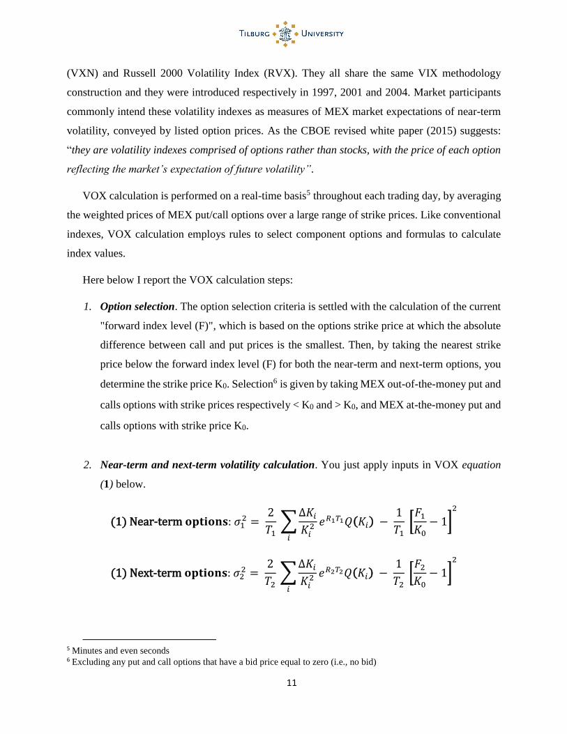
2. Near-term and next-term volatility calculation. You just apply inputs in VOX equation

(1) below.

(1) Near‐term 𝐨𝐩𝐭𝐢𝐨𝐧𝐬: 𝜎12 =

2

𝑇1 ∑

∆𝐾𝑖𝐾𝑖2

𝑖

𝑒𝑅1𝑇1𝑄(𝐾𝑖) − 1

𝑇1 [𝐹1𝐾0− 1]

2

(1) Next‐term 𝐨𝐩𝐭𝐢𝐨𝐧𝐬: 𝜎22 =

2

𝑇2 ∑

∆𝐾𝑖𝐾𝑖2

𝑖

𝑒𝑅2𝑇2𝑄(𝐾𝑖) − 1

𝑇2 [𝐹2𝐾0− 1]

2

5 Minutes and even seconds 6 Excluding any put and call options that have a bid price equal to zero (i.e., no bid)

12

With:

σ : 𝑉𝑂𝑋

100 → 𝑉𝑂𝑋 = σ * 100

T : Time to expiration

F : Forward index level

𝑲𝟎 : First strike price below F

𝑲𝒊 : Strike price of the ith out-of-the-money option; a call if 𝐾𝑖> 𝐾0; and a put if

𝐾𝑖< 𝐾0; both put and call if 𝐾𝑖= 𝐾0

∆𝑲𝒊 : Interval between strike prices - half the difference between the strike on

either side of 𝐾𝑖

𝑸(𝑲𝒊) : The midpoint of the bid-ask spread for each option with strike 𝐾𝑖

3. VOX index level. You multiply by 100 the square root of the 30-day weighted average of

𝜎12 and 𝜎2

2. The process is described by VOX equation (1.1) below.

(𝟏. 𝟏) 𝑽𝑶𝑿 = 100 × √[𝑇1 𝜎12 (𝑁𝑇2 − 𝑁30

𝑁𝑇2 − 𝑁𝑇1) + 𝑇2 𝜎2

2 (𝑁30 − 𝑁𝑇1𝑁𝑇2 − 𝑁𝑇1

)] × 𝑁365𝑁30

With:

𝑵𝑻𝟏 : number of minutes to settlement of the near-term options

𝑵𝑻𝟐 : number of minutes to settlement of the next-term options

𝑵𝟑𝟎 : number of minutes in a 30 days

𝑵𝟑𝟔𝟓 : number of minutes in a 365-day year

3.2. Market Equity Indexes (MEX)

Dow Jones Industrial Average (DJIA)

Dow Jones Industrial Average index is a price-weighted average of the highest 30 stock price

companies traded on the New York Stock Exchange and the Nasdaq. S&P Dow Jones Indices,

13

controlled by McGraw-Hill Financial, provides it. This index represents the most famous of the

Dow Averages, being the second oldest U.S. market index (The Wall Street Journal started

publishing it every day from Oct. 7, 1896). In 1916, DJIA included up to twenty stocks, then

thirty in 1928 and it currently holds the same number. It is expected to track the performance of

the U.S industrial sector in an overall way.

Investing in DJIA is quite easy, since a great variety of financial securities is provided and

largely traded: ETFs, futures and options contracts. Indeed, stock DJIA components are very

liquid and widely held by both individual and institutional investors. This gives the index a

considerable “timeliness”, which means that the index is based at any point in time on very recent

transactions. Its calculation is given by the sum of all the thirty stock prices divided the “Dow

Divisor”. This last term refers to a number, provided and periodically updated by S&P Dow Jones

Indices, which is committed to keep the index historical continuity by accounting for stock splits,

spinoffs and changes among the DJIA stock components. Formula is described in the next page

by equation (2).

(𝟐) 𝑫𝑱𝑰𝑨 = ∑ 𝑆𝑡𝑜𝑐𝑘 𝑝𝑟𝑖𝑐𝑒𝑖30𝑖

𝐷𝑜𝑤 𝐷𝑖𝑣𝑖𝑠𝑜𝑟

Nasdaq 100 (NDX)

Nasdaq 100 is a modified capitalization-weighted index made by the one-hundred largest

non-financial companies listed on the Nasdaq stock exchange. It was introduced on January 31,

1985 by the Nasdaq and it was first limited to U.S companies. Then, after 1998, also foreign

companies started to be admitted but they had to respect stringent restrictions. NDX stock

components belong to Industrial, Technology, Retail, Telecommunication, Biotechnology,

Health Care, Transportation, Media and Service sectors.

NDX derivatives market is a very deep one, with high trading volumes at the exchange. The

same is for its main ETF that in August 2012 was the third most actively traded exchange-traded

product in the world. Nasdaq rebalances this index just once a year. They do so by reviewing

NDX constituents, making out-of-the-index evaluations, provisions and ranking appropriate

companies. Its basic structure is given by the formula of a modified capitalization-weighted

14

method. The term “modified” means that the largest stocks are stopped to a maximum weight

percentage of the total stock index, and the surplus weight it is equally reallocated among the

stocks under that percentage. Formula is described below by equation (3).

(𝟑) 𝑵𝑫𝑿 = ∑ 𝑃𝑖,1𝑖 ∗ 𝑄𝑖,0∑ 𝑃𝑖,0𝑖 ∗ 𝑄𝑖,0

With:

𝑷𝒊,𝟎= Price at base time 0 of the component stock

𝑷𝒊,𝟏= Price at current time 1 of the component stock

𝑸𝒊,𝟎 = Quantity at base time 0 of the component stock

Russell 2000 (RVX)

Russell 2000 is a free-float capitalization-weighted index, composed by (approximately) the

two thousands companies with the smallest market capitalization of the Russell 3000 index.

Introduced by Russell Investments researchers in 1984, it reached a wide success through the

years being commonly used by mutual funds as a benchmark for small-cap stocks in the U.S and

as measure of the small-caps total performance to the one of mid-caps. Indeed, RVX is generally

recognized as the most objective barometer of global small-caps, representing around the 10%

of Russell 3000 total market capitalization. RVX stock constituents are clustered in the Financial

Services, Consumer Discretionary, Producer Durables, Technology and Health Care sectors.

RVX composition is annually adjusted to avoid larger stocks misrepresent performance and

characteristics of the true small-cap block. Moreover, being a free-float adjusted index, it just

includes those stocks that are tradable by the general public of investors (excluding government,

large corporate and large private holdings). Formula is described below by equation (4).

(𝟒) 𝑹𝑽𝑿 = ∑ 𝑃𝑖,1𝑖 ∗ 𝑄𝑖,0∑ 𝑃𝑖,0𝑖 ∗ 𝑄𝑖,0

With:

𝑷𝒊,𝟎= Price at base time 0 of the component stock

15

𝑷𝒊,𝟏= Price at current time 1 of the component stock

𝑸𝒊,𝟎 = “Free-float” adjusted quantity at base time 0 of the component stock

4. Data Building

I collect data from CBOE and Yahoo-finance databases. I start data-collection from the first

date available for each index contained in VOX and I begin from there to collect observations of

corresponding MEX dates7. I do so to have the same corresponding number of observations for

each couple of indexes. The final date of each couple of indexes is the same and it is around mid-

2014 (to leave one year for out-of-the-sample estimations)8. The purpose of having updated and

longer as possible samples is to maximize the statistical accuracy of my results9. Starting and final

dates for each index are reported below in Table 1.1.

Table 1.1

VOX MEX Periods

DJIA Volatility Index (VXD) Dow Jones Industrial

Average Index (DJIA) 10/07/1997 – mid-2014

Nasdaq 100 Volatility Index

(VXN) Nasdaq 100 Index (NDX) 02/01/2001 – mid-2014

Russell 2000 Volatility Index

(RVX) Russell 2000 Index (RUT) 01/02/2004 – mid-2014

From daily-adjusted closing prices of each MEX index at time t, I start to calculate daily rate

of returns. Therefore, I compute the natural logarithm for each day and I multiply it by10 100. The

formula is described in the next page by equation (5).

7 I collect data in this way, since indexes inside MEX are far older than their corresponding ones inside VOX 8 When the out-of-the-sample estimations is meaningless, I extend the final date to 2015. 9 I ignore holidays and weekends 10 This way I will have the exact type of numbers in my time-series

16

(𝟓) 𝑴𝑬𝑿𝒕 = 𝑙𝑛 (𝑀𝐸𝑋𝑡𝑀𝐸𝑋𝑡−1

) × 100

Since I am interested in MEX future n-day volatility, I need to calculate and annualize it11. The

process is described below by equation (6).

(𝟔) 𝑴𝑬𝑿. 𝑽𝒕;𝒔;𝒏 =

{

√∑[𝑀𝐸𝑋𝑡+𝑠;𝑖 − (∑

𝑀𝐸𝑋𝑡+𝑠;𝑖𝑛 + 1

𝑛

𝑖=0

)]

2𝑛

𝑖=0}

× √252

With:

t = current date

n = future trading days from the current date, so the volatility period length

s = number of trading days that must be subtracted or added (±) to the current date

t in order to shift the volatility calculation starting point (if 0 it is just the current

date t)

The method I employ to estimate linear regression parameters is the Ordinary Least Square

(OLS). Representative equation is given below by equation (a).

(𝐚) 𝒀 = 𝜶 + 𝜷 ∗ 𝑿 + 𝜺

5. Over VOX and MEX relationship: regression analysis

Volatility indexes represent a measure of market expectations over the next-future volatility of

their respective set of equity indexes. The key driver of this kind of index is the implied volatility12

of options taken into calculation. The underlying assumption in using VOX, as MEX volatility

forecast tool, is that investor sentiment has some predictive power over future short-term market

movements. This is a reasonable assumption, since participants translate their beliefs in market

11 I do so because, according to CBOE methodology, VOX indexes are annualized 12 According to the Black-Scholes Formula

17

transactions thus in market movements. Therefore, I expect a strong relationship between VOX

and MEX future short-term volatility. This relationship should bring out a good forecasting power

of VOX, or at least good enough to justify its large use by market participants. I perform a set of

OLS linear regression models with different MEX volatility periods and calculation starting points.

I do so in order to statistically catch the underlying relationship between VOX and MEX future

volatility and to assess which is the best one.

5.1. VOX and MEX future 22-day volatility: reference model

I directly start with an investigation over VOX and MEX future 22-day volatility relationship,

since according to CBOE this should be the “unique” one13. Its reliability is the main driver of the

market participants’ use. I postulate linear regression Model 1 as my reference model, with MEX

future 22-day (n =22) volatility as time interval and s = 0 (volatility calculation starting point the

same VOX day). I put MEX future volatility and VOX respectively as my dependent and

independent variable. Formula is described below by equation (1.a).

𝐌𝐨𝐝𝐞𝐥 𝟏 ∶

(𝟏. 𝐚) 𝑴𝑬𝑿. 𝑽𝒕;𝟎;𝟐𝟐 = 𝛼 + 𝛽 ∗ 𝑽𝑶𝑿𝒕 + 𝜀𝑡

Estimated parameters and t-stat coefficients (in brackets) summary are listed below.

Dow Jones Industrial Average, from 10/07/1997 to 06/01/2014, (4176 observations)

(𝟏. 𝐚) 𝑫𝑱𝑰𝑨. 𝑽𝒕;𝟎;𝟐𝟐 = −1.46 + 0.88 ∗ 𝑽𝑿𝑫𝒕 (-5.47) (73.38)

Nasdaq 100, from 02/02/2001 to 06/01/2014, (3350 observations)

(𝟏. 𝐚) 𝑵𝑫𝑿. 𝑽𝒕;𝟎;𝟐𝟐 = −𝟏. 𝟕𝟕 + 𝟎. 𝟗𝟑 ∗ 𝑽𝑿𝑵𝒕 (-6.02) (94.72)

Russell 2000, from 01/02/2004 to 06/01/2014, (2619 observations)

(𝟏. 𝐚) 𝑹𝑼𝑻. 𝑽𝒕;𝟎;𝟐𝟐 = −𝟒. 𝟏𝟒 + 𝟏. 𝟎𝟑 ∗ 𝑹𝑽𝑿𝒕 (-9.93) (69.44)

13 It is the one stated by Whaley, together with Goldman Sachs, in the VIX White Paper (2003)

18

I provide R^2 and correlation coefficients summary in Table 2 below.

Table 2

Index R^2 Correlation

Dow Jones Industrial Average 56.34% 75.05%

Nasdaq 100 72.82% 85.83%

Russell 2000 64.82% 80.51%

The first thing to notice is that all Model 1 regression coefficients are highly significant, at any

level of confidence. Moreover, R^2 and correlation coefficients are generally quite high. Thus,

VOX seems to show a good forecast power over MEX future n=22 volatility. In set of Figures 1.1,

I show scatter plots of Model 1 with interpolation lines according to equation (1.a). I test the VOX

goodness in predicting MEX future n=22 volatility with Model 1, by performing an out-of-the-

sample estimation for one year data (from June 2014 to June 2015). I estimate MEX future 22-day

volatility using parameters I found for each index with regression Model 1 and I compare it with

the out-of-the-sample real MEX future 22-day volatility. Results are shown in set of Figures 1.2.

The out-of-the-sample extrapolation leads to poor results, indeed, the average correlation

coefficients between estimated and real MEX future n=22 volatility is around 28%. Moreover, I

first test for variance similarity (F-test) and then for average similarity (t-test). I always reject, at

any confidence level, the null hypothesis of variance similarity for each couple of estimated versus

real MEX future n=22 volatility. For average similarity, results are mixed:

For Dow Jones estimated versus real future n=22 volatility, I reject the null hypothesis at a

5% level of confidence but not at 1%

For Nasdaq 100 estimated versus real future n=22 volatility I cannot reject the null

hypothesis at any level of confidence

For Russell 2000 estimated versus real future n=22 volatility I reject the null hypothesis at

any level of confidence

Anyway, these results should be interpreted with a more precise knowledge of the empirical

and theoretical (normal) distribution of real future n=22 volatility. This is part of chapter 6.

19

5.2. VOX and MEX future 22-day volatility: VOX past 22-day volatility as

additional independent variable

In order to catch any incremental explanatory power from the simple Model 1, I add VOX past

22-day volatility as second independent variable. The assumption under this addition is that past

one-month levels of “fear” could affect future market movements, so like checking for a market’s

past “fear” memory as a future market volatility driver. I call Model 2 this model with the

additional independent variable. Formula is given by equation (1.b) below.

𝐌𝐨𝐝𝐞𝐥 𝟐:

(𝟏.𝐛) 𝑴𝑬𝑿. 𝑽𝒕;𝟎;+𝟐𝟐 = 𝛼 + 𝛽1 ∗ 𝑽𝑶𝑿𝒕 + 𝛽2 ∗ 𝑽𝑶𝑿. 𝑽𝒕;−𝟐𝟐;+𝟐𝟐 + 𝜀𝑡

I construct VOX past 22-day volatility exactly as I have done for MEX one with equation (5).

Therefore, I calculate daily returns according to the formula described below by equation (7).

(𝟕) 𝑽𝑶𝑿𝒕 = 𝑙𝑛 (𝑉𝑂𝑋𝑡𝑉𝑂𝑋𝑡−1

) × 100

Volatility formula, this time with s = -22, is described by equation (8) below.

(𝟖) 𝑽𝑶𝑿. 𝑽𝒕;𝒔;𝒏 =

{

√∑[𝑉𝑂𝑋𝑡+𝑠;𝑖 − (∑

𝑉𝑂𝑋𝑡+𝑠;𝑖𝑛 + 1

𝑛

𝑖=0

)]

2𝑛

𝑖=0}

× √252

Estimated parameters, t-stat coefficients (in brackets) and R^2-correlation summary are shown

below:

Dow Jones Industrial Average, from 11/07/1997 to 06/01/2014, (4154 observations) :

(𝟏.𝐛) 𝑫𝑱𝑰𝑨. 𝑽𝒕;𝟎;+𝟐𝟐 = −1.12 + 0.81 ∗ 𝑽𝑿𝑫𝒕 + 0.03 ∗ 𝑽𝑿𝑫. 𝑽𝒕;−𝟐𝟐;+𝟐𝟐

(-4.07) (44.79) (5.23)

Nasdaq 100, from 03/07/2001 to 06/01/2014, (3328 observations) :

(𝟏.𝐛) 𝑵𝑫𝑿. 𝑽𝒕;𝟎;+𝟐𝟐 = −1.83 + 0.73 ∗ 𝑽𝑿𝑵𝒕 + 0.13 ∗ 𝑽𝑿𝑵. 𝑽𝒕;−𝟐𝟐;+𝟐𝟐

(-7.30) (74.47) (36.13)

20

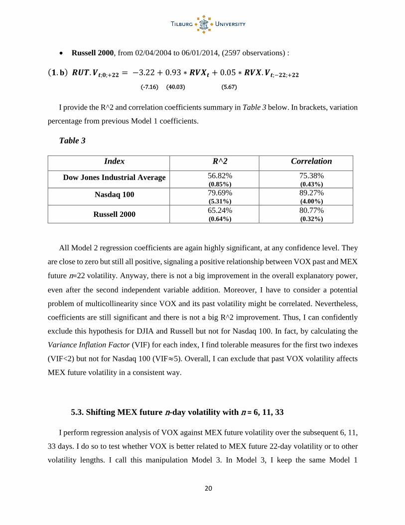
Russell 2000, from 02/04/2004 to 06/01/2014, (2597 observations) :

(𝟏.𝐛) 𝑹𝑼𝑻. 𝑽𝒕;𝟎;+𝟐𝟐 = −3.22 + 0.93 ∗ 𝑹𝑽𝑿𝒕 + 0.05 ∗ 𝑹𝑽𝑿. 𝑽𝒕;−𝟐𝟐;+𝟐𝟐

(-7.16) (40.03) (5.67)

I provide the R^2 and correlation coefficients summary in Table 3 below. In brackets, variation

percentage from previous Model 1 coefficients.

Table 3


Dow Jones Industrial Average 56.82% (0.85%)

75.38% (0.43%)

Nasdaq 100 79.69% (5.31%)

89.27% (4.00%)

Russell 2000 65.24% (0.64%)

80.77% (0.32%)

All Model 2 regression coefficients are again highly significant, at any confidence level. They

are close to zero but still all positive, signaling a positive relationship between VOX past and MEX

future n=22 volatility. Anyway, there is not a big improvement in the overall explanatory power,

even after the second independent variable addition. Moreover, I have to consider a potential

problem of multicollinearity since VOX and its past volatility might be correlated. Nevertheless,

coefficients are still significant and there is not a big R^2 improvement. Thus, I can confidently

exclude this hypothesis for DJIA and Russell but not for Nasdaq 100. In fact, by calculating the

Variance Inflation Factor (VIF) for each index, I find tolerable measures for the first two indexes

(VIF<2) but not for Nasdaq 100 (VIF≈5). Overall, I can exclude that past VOX volatility affects

MEX future volatility in a consistent way.

5.3. Shifting MEX future n-day volatility with n = 6, 11, 33

I perform regression analysis of VOX against MEX future volatility over the subsequent 6, 11,

33 days. I do so to test whether VOX is better related to MEX future 22-day volatility or to other

volatility lengths. I call this manipulation Model 3. In Model 3, I keep the same Model 1

21

independent variable and I just change the volatility lengths (n=6, 11, 33). I report regressions

results in Table 4 below.

Table 4

Index Regression with different n R^2 Corr.

Dow Jones Industrial

Average

from 10/07/1997 to 06/2014

𝑫𝑱𝑰𝑨. 𝑽𝒕;𝟎;𝟔 = −4.33 + 1.00 ∗ 𝑽𝑿𝑫𝒕 (-14.34) (73.00) 55.98 % 74.82 %

𝑫𝑱𝑰𝑨. 𝑽𝒕;𝟎;𝟏𝟏 = −3.73 + 0.98 ∗ 𝑽𝑿𝑫𝒕 (-14.34) (83.70) 62.60 % 79.12 %

𝑫𝑱𝑰𝑨. 𝑽𝒕;𝟎;𝟑𝟑 = −0.22 + 0.83 ∗ 𝑽𝑿𝑫𝒕 (-0.83) (68.68) 53.12 % 72.88 %

Nasdaq 100

from 02/02/2001 to 06/2014

𝑵𝑫𝑿.𝑽𝒕;𝟎;𝟔 = −4.16 + 0.99 ∗ 𝑽𝑿𝑵𝒕 (-11.34) (81.68) 66.49 % 81.54 %

𝑵𝑫𝑿.𝑽𝒕;𝟎;𝟏𝟏 = −3.19 + 0.97 ∗ 𝑽𝑿𝑵𝒕 (-10.26) (94.15) 72.53 % 85.16 %

𝑵𝑫𝑿.𝑽𝒕;𝟎;𝟑𝟑 = −0.58 + 0.88 ∗ 𝑽𝑿𝑵𝒕 (-1.97) (89.92) 70.75 % 84.11 %

Russell 2000

from 01/02/2004 to 06/2014

𝑹𝑼𝑻. 𝑽𝒕;𝟎;𝟔 = −8.00 + 1.15 ∗ 𝑹𝑽𝑿𝒕 (-16.87) (68.33) 63.95 % 79.97 %

𝑹𝑼𝑻. 𝑽𝒕;𝟎;𝟏𝟏 = −6.47 + 1.11 ∗ 𝑹𝑽𝑿𝒕 (-15.44) (74.40) 67.82 % 82.35 %

𝑹𝑼𝑻. 𝑽𝒕;𝟎;𝟑𝟑 = −2.50 + 0.97 ∗ 𝑹𝑽𝑿𝒕 (-5.85) (63.97) 61.11 % 78.17 %

I provide scatter plots for each volatility period, with linear interpolations, in set of Figures 2.1. I

graphically summarize R^2 and correlation coefficients, including those of Model 1, respectively

in Figure 2.2 and 2.3.

Regression parameters are significant at any confidence level, except for DJIA and NDX n=33.

What is worth to notice is that R^2 and correlation coefficients (together with t-stats), gradually

decline with volatility lengths greater than 11 days. I conclude that VOX seems to better predict

MEX future 11-day volatility. Thus, surpassing the commonly accepted claim about VOX as

predictor of the future MEX 22-day volatility. These results are confirmed by performing an out-

of-the-sample extrapolation for the period 2014-2015, using equations retrieved before. Graphs of

22

each extrapolation are shown in set of Figures 2.4. I graphically summarize correlation coefficients

of the out-of-the-sample extrapolation in Figure 2.5.

The out-of-the-sample extrapolation leads to better results than those of the previous

extrapolation (Model 1). The average of correlation coefficients, between estimated and real MEX

future volatility, is around 40% for n=6 and n=11 steadily declining to 28% and 23% for n=22 and

n=33. I also perform variance similarity test (F-test) and then average similarity test (t-test). I

summarize results in Table 5 below, where the word “rejected” refers to the null hypothesis at any

confidence level.

Table 5

F-test/t-test n=6 n=11 n=33


Average Rejected/Rejected Rejected/Rejected

Rejected/Not

Rejected

Nasdaq 100 Rejected/Rejected Rejected/Not Rejected Not Rejected/Not

Rejected

Russell 2000 Rejected/Not

Rejected Rejected/Not Rejected Rejected/Rejected

5.4. VOX and MEX future 22-day volatility: shifting MEX volatility calculation

starting point with s = ± 11, 22, 33 days

As I have showed, results surpass the commonly accepted issue of VOX as predictor of MEX

future 22-day volatility. I find significant coefficients and higher levels of R^2 and correlation,

when I reduce MEX volatility period to either 6 or 11 days.

Anyway, in order to explore the best relationship between these two variables I have to do a

further step. This time, I keep the reference volatility period (n=22) and I let the MEX volatility

calculation starting point vary in the past and in the future (in regards of VOX current date t). This

variation implies that I start to calculate MEX volatility 11, 22, 33 days backwards and forwards.

So, for example, if the VOX current date is 1st April and I set s=11 and n =22, I start to calculate

23

volatility at 15th April and I end 15th May14. I call this manipulation Model 4. In Model 4, I keep

the same Model 1 independent variable and I just change the volatility calculation starting point

(s=±11, 22, 33 days). I report regressions results in Table 6 below and in the next page.

Table 6

Index Regression with different s R^2 Corr.


Average

from 10/07/1997 to 06/2014

𝑫𝑱𝑰𝑨. 𝑽𝒕;𝟏𝟏;𝟐𝟐 = 1.36 + 0.74 ∗ 𝑽𝑿𝑫𝒕 (4.34) (52.61) 40.00% 63.19%

𝑫𝑱𝑰𝑨. 𝑽𝒕;𝟐𝟐;𝟐𝟐 = 3.85 + 0.62 ∗ 𝑽𝑿𝑫𝒕 (11.15) (40.02) 27.87% 52.79%

𝑫𝑱𝑰𝑨. 𝑽𝒕;𝟑𝟑;𝟐𝟐 = 5.87 + 0.52 ∗ 𝑽𝑿𝑫𝒕 (16.07) (31.84) 19.66% 44.34%

𝑫𝑱𝑰𝑨. 𝑽𝒕;−𝟏𝟏;𝟐𝟐 = −4.37 + 1.03 ∗ 𝑽𝑿𝑫𝒕 (-22.37) (116.18) 76.38% 87.39%

𝑫𝑱𝑰𝑨. 𝑽𝒕;−𝟐𝟐;𝟐𝟐 = −4.36 + 1.03 ∗ 𝑽𝑿𝑫𝒕 (-22.48) (117.0) 76.62% 87.53%

𝑫𝑱𝑰𝑨. 𝑽𝒕;−𝟑𝟑;𝟐𝟐 = −2.81 + 0.96 ∗ 𝑽𝑿𝑫𝒕 (-12.0) (90.0) 66.00% 81.22%

Nasdaq 100

from 02/02/2001 to 06/2014

𝑵𝑫𝑿.𝑽𝒕;𝟏𝟏;𝟐𝟐 = 0.17 + 0.85 ∗ 𝑽𝑿𝑵𝒕 (0.50) (74.0) 62.42% 79.00%

𝑵𝑫𝑿.𝑽𝒕;𝟐𝟐;𝟐𝟐 = 2.05 + 0.77 ∗ 𝑽𝑿𝑵𝒕 (5.43) (61.87) 53.52% 73.15%

𝑵𝑫𝑿.𝑽𝒕;𝟑𝟑;𝟐𝟐 = 4.00 + 0.69 ∗ 𝑽𝑿𝑵𝒕 (10.09) (53.01) 45.88% 67.73%

𝑵𝑫𝑿.𝑽𝒕;−𝟏𝟏;𝟐𝟐 = −4.37 + 1.03 ∗ 𝑽𝑿𝑵𝒕 (-22.37) (116.18) 85.13% 92.27%

𝑵𝑫𝑿.𝑽𝒕;−𝟐𝟐;𝟐𝟐 = −4.00 + 1.02 ∗ 𝑽𝑿𝑵𝒕 (-18.37) (139.44) 85.31% 92.36%

𝑵𝑫𝑿.𝑽𝒕;−𝟑𝟑;𝟐𝟐 = −2.91 + 0.99 ∗ 𝑽𝑿𝑵𝒕 (-10.77) (108.0) 77.91% 88.26%

𝑹𝑼𝑻. 𝑽𝒕;𝟏𝟏;𝟐𝟐 = −1.04 + 0.91 ∗ 𝑹𝑽𝑿𝒕 (-2.1) (51.71) 50.65% 71.17%

14 With s = -6 and n = 22, I start from 20th February and I end to 20th January

24

Russell 2000

from 01/02/2004 to 06/2014

𝑹𝑼𝑻. 𝑽𝒕;𝟐𝟐;𝟐𝟐 = 1.64 + 0.80 ∗ 𝑹𝑽𝑿𝒕 (3.00) (41.4)

39.78% 63.07%

𝑹𝑼𝑻. 𝑽𝒕;𝟑𝟑;𝟐𝟐 = 5.16 + 0.67 ∗ 𝑹𝑽𝑿𝒕 (8.52) (31.38) 27.60% 52.53%

𝑹𝑼𝑻. 𝑽𝒕;−𝟏𝟏;𝟐𝟐 = −7.93 + 1.17 ∗ 𝑹𝑽𝑿𝒕 (-28.71) (120.0) 84.55% 91.95%

𝑹𝑼𝑻. 𝑽𝒕;−𝟐𝟐;𝟐𝟐 = −7.87 + 1.17 ∗ 𝑹𝑽𝑿𝒕 (-28.58) (120.0) 84.60% 91.97%

𝑹𝑼𝑻. 𝑽𝒕;−𝟑𝟑;𝟐𝟐 = −5.9 + 1.1 ∗ 𝑹𝑽𝑿𝒕 (-16.61) (87.11) 74.44% 86.28%

I graphically summarize R^2 and correlation coefficients of Model 4, including those of Model

1 (s=0) and those of my reference paper (S&P500), respectively in Figure 3.1 and Figure 3.2.

I observe the best relationship between VOX and MEX volatility, when I shift the MEX

volatility calculation starting point 22-day backwards. In other words, past one-month volatility of

MEX is well related to VOX levels. This relationship implies that MEX one-month volatility is a

good predictor of VOX. This finding is enforced by the fact that is applicable for each index

contained in MEX, with average R^2 and correlation coefficients of respectively 82% and 90%.

Each regression coefficient, of regressions with s=-22, is highly significant. Moreover, results are

similar to those of my reference paper, confirming an underlying relationship that does not depend

on indexes idiosyncrasies but rather on VIX methodology. From this superior performance, I can

conclude that VOX is more reflective of recent historical MEX volatility. Thus, instead of

predicting future MEX volatility, VOX is better “predicted” from MEX past volatility.

5.4.1 VOX and MEX past 22-day volatility: inverse regression

From Model 4, I show that VOX better reflects recent MEX one-month volatility rather than

predicting its future one. This finding completely reverts the commonly accepted view about VOX

as predictor of MEX future one-month volatility and it suggests how MEX past one-month

volatility explains actual VOX. Therefore, to further analyze this relationship, I directly regress

VOX against MEX past 22-day volatility. This means that I put VOX as dependent variable and

25

MEX past 22-day volatility as independent one. Of course, I expect different regression

coefficients but the same levels or R^2 and correlation. I call this model, Model 5.

𝐌𝐨𝐝𝐞𝐥 𝟓 ∶

𝑽𝑶𝑿𝒕 = 𝛼 + 𝛽 ∗ 𝑴𝑬𝑿. 𝑽𝒕;−𝟐𝟐;𝟐𝟐 + 𝜀𝑡

Estimated parameters, t-stat coefficients (in brackets) are shown below:

Dow Jones Industrial Average, from 11/24/1997 to 07/01/2014, (4164 observations) :

𝑽𝑿𝑫𝒕 = 8.00 + 0.73 ∗ 𝑫𝑱𝑰𝑨. 𝑽𝒕;−𝟐𝟐;𝟐𝟐 (65.62) (117.23)

Nasdaq 100, from 03/22/2001 to 07/01/2014, (3337 observations) :

𝑽𝑿𝑵𝒕 = 7.34 + 0.82 ∗ 𝑵𝑫𝑿. 𝑽𝒕;−𝟐𝟐;𝟐𝟐 (44.74) (137.26)

Russell 2000, from 02/20/2004 to 07/01/2014, (2606 observations) :

𝑹𝑽𝑿𝒕 = 9.68 + 0.61 ∗ 𝑹𝑼𝑻. 𝑽𝒕;−𝟐𝟐;𝟐𝟐 (60.85) (119.6)

In Table 7 below, I provide the R^2 and correlation coefficients summary.

Table 7



Nasdaq 100 85% 92.2%

Russell 2000 84.6% 92%

All Model 5 regression coefficients are highly significant, at any level of confidence. Moreover,

R^2 and correlation coefficients are as high as expected. It is worth to notice that with this linear

model, it is confidently possible to replicate actual levels of VOX. In set of Figures 4.1, I provide

scatter plots to show how Model 5 confirms findings of Model 4 (s=-22). To further test the

26

goodness of this relationship, I perform an out-of-the-sample extrapolation (2014-2015 period)

using equations of Model 5. Results are shown in set of Figures 4.2.

The out-of-the-sample extrapolation leads to good results. The average of correlation

coefficients of estimated and real VOX is around 54%, which is almost double than that of the

reference model (Model 1). Anyway, tests on variance (F-test) and average (t-test) similarity lead

to different results:

I always reject at any level of confidence average null hypothesis

I always reject at any level of confidence variance null hypothesis, except from:

Russell 2000 at any level of confidence

Nasdaq 100 at 10% confidence level

5.5. VOX and MEX volatility: combination of varying MEX volatility calculation

starting points (s = - 11, 22, 33) and MEX future n-day volatility periods (n = 6, 11, 33)

From Model 5, I observe that VOX better reflects past MEX volatility instead of future one

and that shorter MEX volatility periods are better related to VOX actual levels. In either direction,

I find that the theoretical relationship between VOX and MEX future 22-day volatility is not the

best one.

In this chapter, I try to exploit previous insights. This means that I start to calculate MEX

volatility just into the past (s=- 11, 22, 33) and I combine those starting points with different

volatility periods (n=6, 11, 33) for each index. My goal is to find the unanimously best relationship

by exploring all the possible combinations using previous insights. I call this manipulation, Model

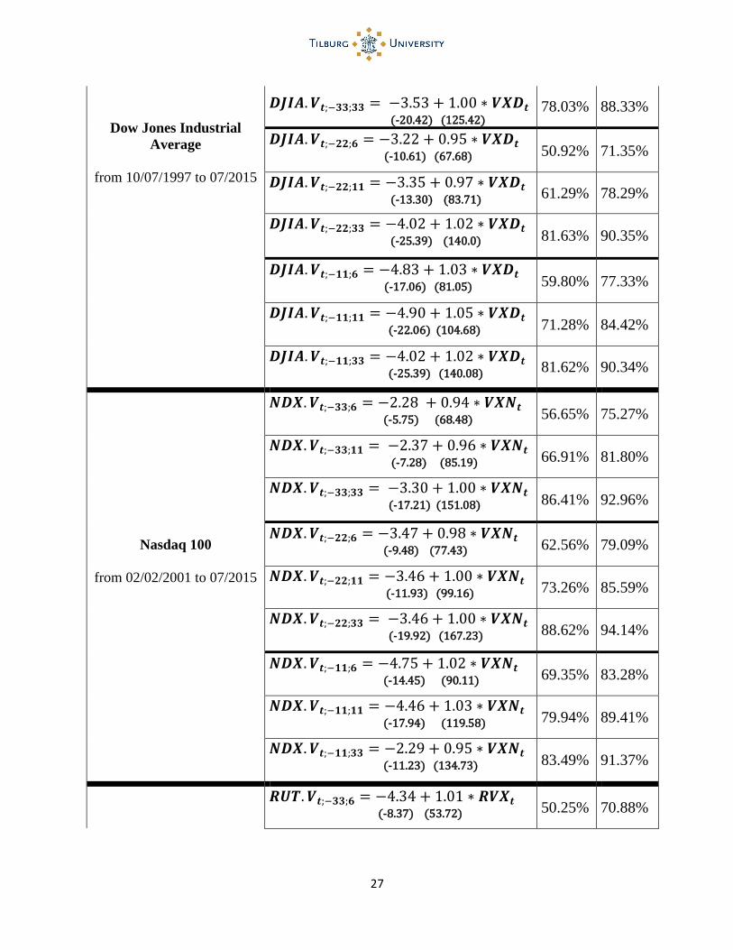
6. I report regressions results for the full sample in Table 8, below and in the next pages.

Table 8

Index Regression with increasing s and n R^2 Corr.

𝑫𝑱𝑰𝑨. 𝑽𝒕;−𝟑𝟑;𝟔 = −1.69 + 0.87 ∗ 𝑽𝑿𝑫𝒕 (-5.17) (57.91) 43.17% 65.70%

𝑫𝑱𝑰𝑨. 𝑽𝒕;−𝟑𝟑;𝟏𝟏 = −1.98 + 0.91 ∗ 𝑽𝑿𝑫𝒕 (-7.17) (70.87) 53.22% 72.95%

27


Average

from 10/07/1997 to 07/2015

𝑫𝑱𝑰𝑨. 𝑽𝒕;−𝟑𝟑;𝟑𝟑 = −3.53 + 1.00 ∗ 𝑽𝑿𝑫𝒕 (-20.42) (125.42)

78.03% 88.33%

𝑫𝑱𝑰𝑨. 𝑽𝒕;−𝟐𝟐;𝟔 = −3.22 + 0.95 ∗ 𝑽𝑿𝑫𝒕 (-10.61) (67.68) 50.92% 71.35%

𝑫𝑱𝑰𝑨. 𝑽𝒕;−𝟐𝟐;𝟏𝟏 = −3.35 + 0.97 ∗ 𝑽𝑿𝑫𝒕 (-13.30) (83.71) 61.29% 78.29%

𝑫𝑱𝑰𝑨. 𝑽𝒕;−𝟐𝟐;𝟑𝟑 = −4.02 + 1.02 ∗ 𝑽𝑿𝑫𝒕 (-25.39) (140.0) 81.63% 90.35%

𝑫𝑱𝑰𝑨. 𝑽𝒕;−𝟏𝟏;𝟔 = −4.83 + 1.03 ∗ 𝑽𝑿𝑫𝒕 (-17.06) (81.05) 59.80% 77.33%

𝑫𝑱𝑰𝑨. 𝑽𝒕;−𝟏𝟏;𝟏𝟏 = −4.90 + 1.05 ∗ 𝑽𝑿𝑫𝒕 (-22.06) (104.68) 71.28% 84.42%

𝑫𝑱𝑰𝑨. 𝑽𝒕;−𝟏𝟏;𝟑𝟑 = −4.02 + 1.02 ∗ 𝑽𝑿𝑫𝒕 (-25.39) (140.08) 81.62% 90.34%

Nasdaq 100

from 02/02/2001 to 07/2015

𝑵𝑫𝑿.𝑽𝒕;−𝟑𝟑;𝟔 = −2.28 + 0.94 ∗ 𝑽𝑿𝑵𝒕 (-5.75) (68.48) 56.65% 75.27%

𝑵𝑫𝑿.𝑽𝒕;−𝟑𝟑;𝟏𝟏 = −2.37 + 0.96 ∗ 𝑽𝑿𝑵𝒕 (-7.28) (85.19) 66.91% 81.80%

𝑵𝑫𝑿.𝑽𝒕;−𝟑𝟑;𝟑𝟑 = −3.30 + 1.00 ∗ 𝑽𝑿𝑵𝒕 (-17.21) (151.08) 86.41% 92.96%

𝑵𝑫𝑿.𝑽𝒕;−𝟐𝟐;𝟔 = −3.47 + 0.98 ∗ 𝑽𝑿𝑵𝒕 (-9.48) (77.43) 62.56% 79.09%

𝑵𝑫𝑿.𝑽𝒕;−𝟐𝟐;𝟏𝟏 = −3.46 + 1.00 ∗ 𝑽𝑿𝑵𝒕 (-11.93) (99.16) 73.26% 85.59%

𝑵𝑫𝑿.𝑽𝒕;−𝟐𝟐;𝟑𝟑 = −3.46 + 1.00 ∗ 𝑽𝑿𝑵𝒕 (-19.92) (167.23) 88.62% 94.14%

𝑵𝑫𝑿.𝑽𝒕;−𝟏𝟏;𝟔 = −4.75 + 1.02 ∗ 𝑽𝑿𝑵𝒕 (-14.45) (90.11) 69.35% 83.28%

𝑵𝑫𝑿.𝑽𝒕;−𝟏𝟏;𝟏𝟏 = −4.46 + 1.03 ∗ 𝑽𝑿𝑵𝒕 (-17.94) (119.58) 79.94% 89.41%

𝑵𝑫𝑿.𝑽𝒕;−𝟏𝟏;𝟑𝟑 = −2.29 + 0.95 ∗ 𝑽𝑿𝑵𝒕 (-11.23) (134.73) 83.49% 91.37%

𝑹𝑼𝑻. 𝑽𝒕;−𝟑𝟑;𝟔 = −4.34 + 1.01 ∗ 𝑹𝑽𝑿𝒕 (-8.37) (53.72) 50.25% 70.88%

28

Russell 2000

from 01/02/2004 to 07/2015

𝑹𝑼𝑻. 𝑽𝒕;−𝟑𝟑;𝟏𝟏 = −4.87 + 1.05 ∗ 𝑹𝑽𝑿𝒕 (-11.46) (67.82)

61.69% 78.54%

𝑹𝑼𝑻. 𝑽𝒕;−𝟑𝟑;𝟑𝟑 = −6.91 + 1.14 ∗ 𝑹𝑽𝑿𝒕 (-28.96) (121.73) 85.86% 92.66%

𝑹𝑼𝑻. 𝑽𝒕;−𝟐𝟐;𝟔 = −6.16 + 1.08 ∗ 𝑹𝑽𝑿𝒕 (-12.87) (62.25) 57.56% 75.87%

𝑹𝑼𝑻. 𝑽𝒕;−𝟐𝟐;𝟏𝟏 = −6.39 + 1.11 ∗ 𝑹𝑽𝑿𝒕 (-16.66) (69.40) 68.81% 82.95%

𝑹𝑼𝑻. 𝑽𝒕;−𝟐𝟐;𝟑𝟑 = −7.43 + 1.16 ∗ 𝑹𝑽𝑿𝒕 (-34.86) (150.0) 88.73% 94.19%

𝑹𝑼𝑻. 𝑽𝒕;−𝟏𝟏;𝟔 = −8.44 + 1.17 ∗ 𝑹𝑽𝑿𝒕 (-20.05) (76.58) 67.24% 82.00%

𝑹𝑼𝑻. 𝑽𝒕;−𝟏𝟏;𝟏𝟏 = −8.60 + 1.19 ∗ 𝑹𝑽𝑿𝒕 (-27.72) (105.63) 69.64% 89.24%

𝑹𝑼𝑻. 𝑽𝒕;−𝟏𝟏;𝟑𝟑 = −6.12 + 1.11 ∗ 𝑹𝑽𝑿𝒕 (-22.05) (109.92) 80.87% 89.93%

I summarize R^2 and correlation coefficients, for each couple of indexes and combinations, in

Tables from 9 to 11 below and in the next page.

Tables 9 – Dow Jones Industrial Average

DJIA (R^2)

n = 6 n = 11 n = 22 n = 33

s = -33 43,17% 53,22% 65,85% 78,03%

s = -22 50,92% 61,30% 76,61% 81,63%

s = -11 59,81% 71,28% 76,70% 81,62%

s = 0 55,98% 62,60% 56,60% 53,66%

DJIA (Corr)

n = 6 n = 11 n = 22 n = 33

s = -33 65,71% 72,95% 81,15% 88,34%

s = -22 71,36% 78,29% 87,53% 90,35%

s = -11 77,34% 84,43% 87,58% 90,34%

s = 0 74,82% 79,12% 75,23% 73,26%

29

Tables 10 – Nasdaq 100

Tables 11 – Russell 2000

I graphically summarize R^2 and correlation coefficients, including those of Model 1 (s =0 and

n =22), respectively in set of Figures 5.1 and Figures 5.2.

I extended periods to 07/2015, because for these types of variables an out-of-the-sample

extrapolation would not be feasible. I notice that all coefficients are significant, at any level of

confidence. Moreover, as highlighted from graphs, there is a clear evidence of how the best

relationship is described by combination: s=-22 and n=33. This means that VOX best reflects the

past 1 month + future ½ month MEX volatility, showing the highest R^2 and correlation

coefficients. It is evident a path that shows how, fixing the volatility period, estimation goodness

rises up by shortening the volatility calculation period up to 11 days before. It is worth to notice

that VOX slightly better reflects past 33-day volatility (s=-33; n=33) rather than 22-day one (s=-

22; n=22).

NDX (R^2)

n = 6 n = 11 n = 22 n = 33

s = -33 56,66% 66,92% 77,91% 86,42%

s = -22 62,56% 73,27% 85,16% 88,63%

s = -11 69,36% 79,94% 84,76% 83,50%

s = 0 66,98% 72,96% 73,30% 71,42%

NDX (Corr)

n = 6 n = 11 n = 22 n = 33

s = -33 75,27% 81,80% 88,27% 92,96%

s = -22 79,10% 85,60% 92,28% 94,14%

s = -11 83,28% 89,41% 92,06% 91,38%

s = 0 81,84% 85,41% 85,61% 84,51%

RUT (Corr)

n = 6 n = 11 n = 22 n = 33

s = -33 70,89% 78,54% 86,37% 92,66%

s = -22 75,87% 82,96% 92,06% 94,20%

s = -11 82,00% 89,25% 92,13% 89,93%

s = 0 80,04% 82,55% 80,87% 78,67%

RUT (R^2)

n = 6 n = 11 n = 22 n = 33

s = -33 50,25% 61,69% 74,59% 85,86%

s = -22 57,56% 68,82% 84,74% 88,73%

s = -11 67,24% 79,65% 84,88% 80,88%

s = 0 64,07% 68,15% 65,40% 61,90%

30

6. VOX and MEX future 22-day volatility: high and normal volatility

periods

From the analysis performed over the reference model (Model 1), I see a VOX tendency to

overestimate and underestimate MEX future n=22 volatility respectively during normal and high

volatility periods of MEX. In order to check this finding, I sort my datasets into two different

regimes15: high-volatility regime and normal-volatility regime. This sorting is based on MEX

volatility levels during the full sample. With “high-volatility”, I mean greater than two standard

deviations from the mean, so16: 𝑯.𝑽 𝑖𝑓 𝑎𝑛𝑑 𝑜𝑛𝑙𝑦 𝑖𝑓 > 𝝁 + 𝟐 ∗ 𝝈

I perform the same regressions of Model 1, this time using just high-volatility observations for

each index as datasets. Estimated parameters and t-stat coefficients (in brackets) are shown below:

Dow Jones Industrial Average, (212 observations) :

𝐇𝐢𝐠𝐡 𝐩𝐞𝐫𝐢𝐨𝐝𝐬: 𝑫𝑱𝑰𝑨. 𝑽𝒕;𝟎;𝟐𝟐 = 29.29 + 0.50 ∗ 𝑽𝑿𝑫𝒕

(12.72) (8.41)

Nasdaq 100, (232 observations) :

𝐇𝐢𝐠𝐡 𝐩𝐞𝐫𝐢𝐨𝐝𝐬: 𝑵𝑫𝑿. 𝑽𝒕;𝟎;𝟐𝟐 = 57.80 + 0.07 ∗ 𝑽𝑿𝑵𝒕

(16.69) (1.15)

Russell 2000, (99 observations) :

𝐇𝐢𝐠𝐡 𝐩𝐞𝐫𝐢𝐨𝐝𝐬: 𝑹𝑼𝑻. 𝑽𝒕;𝟎;𝟐𝟐 = 57.47 + 0.17 ∗ 𝑹𝑽𝑿𝒕

(10.74) (1.80)

I provide R^2 and correlation coefficients summary in Table 12, below.

Table 12



Nasdaq 100 0.58% 7.62%

Russell 2000 3.25% 18.03%

15 Since it is meaningless to perform an out-of-the-sample extrapolation, I use data updated to 06/2015 16 Of course, “with normal-volatility” I mean all the other. So: 𝑵.𝑽 𝑖𝑓 𝑎𝑛𝑑 𝑜𝑛𝑙𝑦 𝑖𝑓 < 𝝁 + 𝟐 ∗ 𝝈

31

Compared to Model 1, I notice a huge change in sign, magnitude and significance of estimation

coefficients. Indeed, there is basically no predictive power for Nasdaq 100 and Russell 2000 as it

is shown by R^2 and correlations. For Dow Jones, I observe a greater predictive power (even if

poor in an absolute value) and this because volatilities are not as “high” as for the other two indexes.

Anyway, these results are misleading if taken as pure results. Indeed, datasets used are composed

of comprised volatility periods with few observations and often very far one each other.

Notwithstanding limitations, it is useful to highlight the big difference from previous findings.

I catch these differences comparing descriptive statistics for both VOX and MEX future 22-day

volatility. Moreover, I indicate the length of each regime and I show correlation within each period.

In addition, I empirically test the hypothesis that VOX tends to overestimate and underestimate

MEX future 22-day volatility during respectively normal and high volatility periods. I provide the

realization percentages17 of this hypothesis.

Realization percentages for each period are given by formulas of equations (8) and (9) below.

(𝟖) 𝐍𝐨𝐫𝐦𝐚𝐥 𝐩𝐞𝐫𝐢𝐨𝐝𝐬:

𝑛° 𝑜𝑏𝑠. 𝑤𝑖𝑡ℎ𝑖𝑛 𝑝𝑒𝑟𝑖𝑜𝑑 (𝑉𝑂𝑋 > 𝑀𝐸𝑋 𝑓𝑢𝑡. 22 𝑣𝑜𝑙. )

𝑇𝑜𝑡𝑎𝑙 𝑛° 𝑜𝑏𝑠. 𝑤𝑖𝑡ℎ𝑖𝑛 𝑝𝑒𝑟𝑖𝑜𝑑 = %𝑶𝒗𝒆𝒓𝒆𝒔𝒕𝒊𝒎𝒂𝒕𝒆 𝒘𝒊𝒕𝒉𝒊𝒏 𝒑𝒆𝒓𝒊𝒐𝒅

(𝟗) 𝐇𝐢𝐠𝐡 𝐩𝐞𝐫𝐢𝐨𝐝𝐬:

𝑛° 𝑜𝑏𝑠. 𝑤𝑖𝑡ℎ𝑖𝑛 𝑝𝑒𝑟𝑖𝑜𝑑 (𝑉𝑂𝑋 < 𝑀𝐸𝑋 𝑓𝑢𝑡. 22 𝑣𝑜𝑙. )

𝑇𝑜𝑡𝑎𝑙 𝑛° 𝑜𝑏𝑠. 𝑤𝑖𝑡ℎ𝑖𝑛 𝑝𝑒𝑟𝑖𝑜𝑑 = %𝑼𝒏𝒅𝒆𝒓𝒆𝒔𝒕𝒊𝒎𝒂𝒕𝒆 𝒘𝒊𝒕𝒉𝒊𝒏 𝒑𝒆𝒓𝒊𝒐𝒅

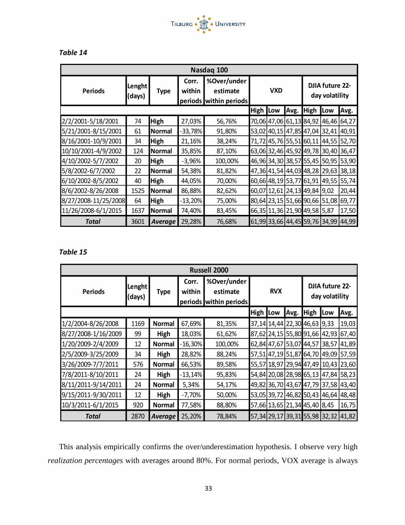
Summaries are shown in the next pages, in Tables from 13 to 15.

17 Realization percentages are called: %Over/underestimate for normal/high period

32

Table 13

PeriodsLenght

(days)Type

Corr.

within

periods

%Over/under

estimate

within periodsHigh Low Avg. High Low Avg.

10/7/1997-8/5/1998 208 Normal 33,69% 90,38% 36,48 17,39 23,14 34,17 9,90 15,97

8/6/1998-8/31/1998 18 High -29,56% 94,44% 42,50 27,87 31,51 42,46 35,34 40,03

9/1/1998-8/15/2001 746 Normal 34,17% 83,91% 42,95 13,47 23,94 34,27 8,50 18,42

8/16/2001-9/10/2001 17 High 43,36% 100,00% 28,36 20,25 23,78 39,21 36,20 37,67

9/17/2001-6/20/2002 192 Normal 31,05% 84,90% 39,86 16,80 23,61 28,81 10,74 18,19

6/21/2002-7/26/2002 25 High -32,64% 84,00% 41,81 24,87 30,36 44,75 34,84 40,72

7/29/2002-8/23/2002 20 Normal 54,54% 100,00% 41,85 28,49 34,12 32,65 24,70 27,78

8/26/2002-10/1/2002 26 High 60,80% 96,15% 40,57 30,71 36,41 48,22 35,40 42,26

10/02/2002-8/18/2008 1480 Normal 79,48% 81,69% 41,10 9,28 16,59 34,38 5,49 13,38

8/19/2008-18/28/2008 72 High 32,95% 83,33% 74,60 18,41 43,89 82,82 35,09 61,80

12/01/2008-1/30/2009 42 Normal -21,22% 100,00% 62,40 34,53 44,00 34,56 26,66 31,19

2/2/2009-3/20/2009 34 High 44,12% 38,24% 47,02 36,37 40,62 45,43 35,27 39,68

3/23/2009-07/11/2011 577 Normal 59,55% 90,12% 40,72 12,77 20,71 33,59 3,90 15,17

7/12/2011-8/8/2011 20 High -9,32% 95,00% 40,49 16,01 21,37 42,51 35,80 39,91

8/09/2011-6/01/2015 951 Normal 78,07% 86,86% 41,45 9,71 15,86 34,58 3,52 12,23

Total 4428 Average 30,60% 87,27% 44,14 21,13 28,66 40,83 22,76 30,29

Dow Jones

VXDDJIA future 22-

day volatility

33

Table 14

Table 15

This analysis empirically confirms the over/underestimation hypothesis. I observe very high

realization percentages with averages around 80%. For normal periods, VOX average is always

PeriodsLenght

(days)Type

Corr.

within

periods

%Over/under

estimate

within periods

High Low Avg. High Low Avg.

1/2/2004-8/26/2008 1169 Normal 67,69% 81,35% 37,14 14,44 22,30 46,63 9,33 19,03

8/27/2008-1/16/2009 99 High 18,03% 61,62% 87,62 24,15 55,80 91,66 42,93 67,40

1/20/2009-2/4/2009 12 Normal -16,30% 100,00% 62,84 47,67 53,07 44,57 38,57 41,89

2/5/2009-3/25/2009 34 High 28,82% 88,24% 57,51 47,19 51,87 64,70 49,09 57,59

3/26/2009-7/7/2011 576 Normal 66,53% 89,58% 55,57 18,97 29,94 47,49 10,43 23,60

7/8/2011-8/10/2011 24 High -13,14% 95,83% 54,84 20,08 28,98 65,13 47,84 58,23

8/11/2011-9/14/2011 24 Normal 5,34% 54,17% 49,82 36,70 43,67 47,79 37,58 43,40

9/15/2011-9/30/2011 12 High -7,70% 50,00% 53,05 39,72 46,82 50,43 46,64 48,48

10/3/2011-6/1/2015 920 Normal 77,58% 88,80% 57,66 13,65 21,34 45,40 8,45 16,75

Total 2870 Average 25,20% 78,84% 57,34 29,17 39,31 55,98 32,32 41,82

RVXDJIA future 22-

day volatility

Russell 2000

PeriodsLenght

(days)Type

Corr.

within

periods

%Over/under

estimate

within periods

High Low Avg. High Low Avg.

2/2/2001-5/18/2001 74 High 27,03% 56,76% 70,06 47,06 61,13 84,92 46,46 64,27

5/21/2001-8/15/2001 61 Normal -33,78% 91,80% 53,02 40,15 47,85 47,04 32,41 40,91

8/16/2001-10/9/2001 34 High 21,16% 38,24% 71,72 45,76 55,51 60,11 44,55 52,70

10/10/2001-4/9/2002 124 Normal 35,85% 87,10% 63,06 32,46 45,92 49,78 30,40 36,47

4/10/2002-5/7/2002 20 High -3,96% 100,00% 46,96 34,30 38,57 55,45 50,95 53,90

5/8/2002-6/7/2002 22 Normal 54,38% 81,82% 47,36 41,54 44,03 48,28 29,63 38,18

6/10/2002-8/5/2002 40 High 44,05% 70,00% 60,66 48,19 53,77 61,91 49,55 55,74

8/6/2002-8/26/2008 1525 Normal 86,88% 82,62% 60,07 12,61 24,13 49,84 9,02 20,44

8/27/2008-11/25/2008 64 High -13,20% 75,00% 80,64 23,15 51,66 90,66 51,08 69,77

11/26/2008-6/1/2015 1637 Normal 74,40% 83,45% 66,35 11,36 21,90 49,58 5,87 17,50

Total 3601 Average 29,28% 76,68% 61,99 33,66 44,45 59,76 34,99 44,99

Nasdaq 100

VXDDJIA future 22-

day volatility

34

above the one of MEX, while for high periods is exactly the opposite. Therefore, it is reasonable

to conclude that VOX tends to systematically underestimate high MEX future 22-day volatility

levels and vice versa for normal ones. I also detect a sudden increase at the end of almost all normal

volatility periods and a proportionally smaller increase of VOX. This finding is confirmed by

observing correlation within periods, which is generally very poor and even negative sometimes,

with averages around 27%. Particularly for high periods, where the average period length is very

short, I observe a great variability of correlation coefficients. This confirms the finding that VOX

reflects past MEX volatility. Thus, for short subsequent periods of different volatility regimes,

VOX predictive power is very poor with also negative correlation coefficients sometimes.

7. VOX and MEX future 22-day volatility: distribution analysis

The final step involves a closer look at VOX and MEX future 22-day volatility distributions.

This is important to understand their statistical characteristics and to enhance awareness of

normality tests. In set of Figures 6.1, I show the empirical distribution of each index by sorting

frequencies for each measure and along the full sample (updated to 06/2015). In the same set of

figures, I also draw theoretical (Normal/Gaussian) distributions for each index, using historical

averages and standard deviations for each index along the full sample.

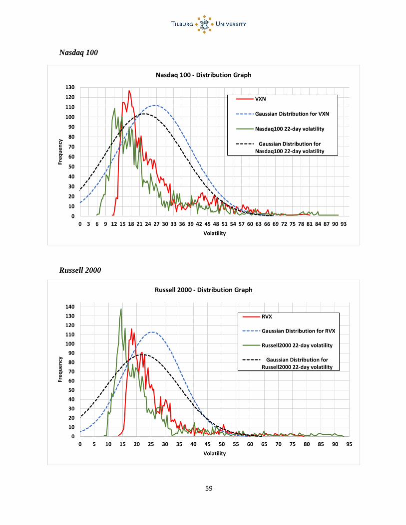
I observe that empirical distributions (for both measures) show fatter tails (leptokurtosis)

compared to Normal ones. Moreover, I notice that empirical MEX future 22-day volatility

distributions show greater kurtosis and skewness compared to those of corresponding VOX.

Indeed, empirical and Normal VOX and MEX future 22-day volatility distributions should be

overlapped if the first is a good predictor of the second one. Empirical distributions are

significantly more skewed than their respective theoretical ones. The same happens across VOX

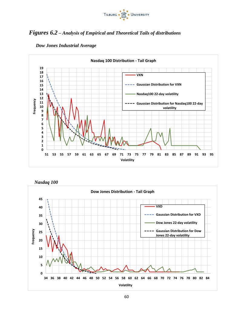
empirical frequencies and MEX empirical ones. I go deep with the analysis the tails18 distributions,

as shown in set of Figures 6.2. The right tail expresses the high-volatility observation frequency,

thus for observations greater than two standard deviations from the mean. As said, I observe “fatter”

empirical tails than those of Normal distributions. Moreover, MEX future 22-day volatility still

exhibits observations over the VOX highest observation and generally higher frequencies for the

18 Of course the one of interest is the right tail since we cannot observe values below 0

35

same VOX highest observations. Finally, I use normality tests for each empirical distribution, in

order to statistically confirm previous findings. I always reject the null19 for each distribution and

each tests performed:

Jarque-Bera

Kolmogorov-Smirnov

Anderson-Darling

Chi-squared

Lilliefors

I provide in Appendix the best fitting distributions, with estimated parameters, for each VOX

and MEX future 22-day volatility empirical distribution.

8. Conclusions

Following the same research methodology used by Vodenska and Chambers (2013) for VIX

analysis and with the most updated datasets available, I analyze the underling relationship between

Dow Jones, Nasdaq 100, Russell 2000 volatilities (MEX) and their respective CBOE volatility

indexes (VOX). Findings in this study show that the commonly accepted view of VOX as predictor

of MEX future 22-day volatility is misleading. Indeed, this view does not reflect nor the true nor

the best relationship between these two measures. Surprisingly, I find superior R^2 and correlation

coefficients when I shift the starting point to calculate MEX future volatility one-month backwards.

In other words, when I regress MEX past 22-day volatility against VOX. I show that VOX has

stronger connections with MEX past 22-day volatility than in regard of MEX future 22-day one,

with average R^2 and correlation coefficients respectively around 82% and 90%. I conclude that

VOX better reflects recent MEX past volatility, instead of predicting MEX future one. I confirm

this finding by directly regressing VOX against MEX past 22-day volatility. Anyway, the

unanimously best relationship arises when calculate MEX volatility one-month backwards with a

volatility length of 33-day, thus regressing VOX against MEX past 1 month + future ½ month

volatility. This selection leads to R^2 and correlation coefficients, respectively around 86% and

19 Null Hypothesis: normality of distribution

36

93%. I go deep with the analysis dividing periods into high and normal ones, according to volatility

levels. I empirically show that during normal volatility regimes VOX tends to overestimate MEX

future 22-day volatility and to underestimate it during high volatility regimes. Results suggest that,

on average, more than 80% of the times over/underestimates are confirmed. I also observe severe

variations of correlation coefficients within periods through each regime and even negatives

sometimes. Finally, I perform a distribution analysis for both VOX and MEX future 22-day

volatility. I analyze their empirical distributions against their respective Normal ones. I also

perform a tail-distribution analysis, and I observe higher levels of kurtosis for each empirical

distribution in regard of their respective theoretical ones. Furthermore, I test for normality and I

always reject the null hypothesis for each empirical distribution. I also observe that MEX future

22-day volatility levels of skewness and kurtosis are higher than their respective VOX ones. This

confirms the finding that VOX tends to underestimate MEX future 22-day volatility during high-

volatility periods, and vice versa. It is worth to notice that all results of this study are exactly the

same of those of Vodenska and Chambers (2013, reference paper) for VIX. Moreover, I always

find the same results for each couple of indexes I analyze, so for VXD, VXN, RVX and their

respective MEX. This indicates that, regardless index idiosyncrasies, CBOE volatility index

methodology is the key to really understand the underlying relationship between these two

financial measures. The reasons why these relationships and behaviors occur are far beyond the

scope of this work. Indeed, the aim of this paper is limited to the description of the underlying

relationship between VOX and MEX volatility and their empirical characteristics. This work is an

effort to complete the statistical analysis over the U.S major equity set of CBOE volatility indexes

started with VIX, and to improve investor awareness and interpretation of this new set of financial

tools.

37

9. References

Poon, Ser-Huang; Granger, Clive W.J., (2003). Forecasting Volatility in Financial Markets:

A Review. Journal of Economic Literature. 41 (62), pp. 478-539.

http://dx.doi.org/10.1257/002205103765762743

David P. Simon, (2003). The Nasdaq Volatility Index During and After the Bubble. The

Journal of Derivatives. 11 (2), pp.9-24. DOI: 10.3905/jod.2003.319213

Charles J. Corrado and Thomas W. Miller, Jr, (2005). The forecast quality of CBOE implied

volatility indexes. Journal of Futures Markets. 25 (4), pp.339–373. DOI: 10.1002/fut.20148

Ralf Becker and Adam Clements, (2007). Are combination forecasts of S&P 500 volatility

statistically superior?. National Centre for Econometric Research. Working paper.

Ralf Becker and Adam Clements, (2009). The jump component of S&P 500 volatility and the

VIX index. Journal of Banking & Finance. 33 (6), pp.1033–1038.

DOI: 10.1016/j.jbankfin.2008.10.015

Robert E. Whaley, (2009). Understanding VIX. Journal of Portfolio Management,

http://dx.doi.org/10.2139/ssrn.1296743

Vodenska, I., & Chambers, W. J. (2013). Understanding the relationship between VIX and

the S&P 500 index volatility. In 26th Australasian Finance and Banking Conference.


http://dx.doi.org/10.1257/002205103765762743



38

Figures 1.1 – Model 1 scatter plots with linear interpolation lines:

Dow Jones Industrial Average

Nasdaq 100

39

Russell 2000

Figures 1.2 – Model 1 out-of-the-sample extrapolation 2014-2015:


0

2

4

6

8

10

12

14

16

18

20

Dow Jones Real vs. Estimated future n=22 Volatility for

2014/15

Estimated future n=22 volatilities Real Future n=22 ann. volatilities

40

Nasdaq 100

Russell 2000

0,00

5,00

10,00

15,00

20,00

25,00

Nasdaq 100 Real vs. Estimated future n=22 Volatility for

2014/15


0,00

5,00

10,00

15,00

20,00

25,00

Russell 2000 Real vs. Estimated future n=22 Volatility for

2014/15


41

Figures 2.1 – Model 3 scatter plots with linear interpolation lines:

Dow Jones n =6, 11, 33

43

Nasdaq 100 n =6, 11, 33

44

Russell 2000 n =6, 11, 33

45

Figure 2.2 – Model 3 graphical summary of R^2 coefficients (including those of Model 1)

50%

55%

60%

65%

70%

75%

n=6 n=11 n=22 (Model 1) n=33

R^2

Dow Jones Industrial Average Nasdaq 100 Russell 2000

46

Figure 2.3 – Model 3 graphical summary of Corr. coefficients (including those of Model 1)

Figures 2.4 – Model 3 out-of-the-sample extrapolation 2014-2015

Dow Jones Real vs. Estimated Volatility with n= 6, 11, 33

70%

72%

74%

76%

78%

80%

82%

84%

86%

88%

90%

n=6 n=11 n=22 (Model 1) n=33

Correlation


0

5

10

15

20

25

30

DowJones Real vs. Estimated n=6 Volatility for 2014/2015

REAL future n=6 ann. volatilities ESTIMATED future N=6 ann. Volatilities

47

0

5

10

15

20

25


REAL future N=11 ann. volatilities ESTIMATED future N=11 ann. volatilities

0

2

4

6

8

10

12

14

16

18

20


REAL future N=33 ann. volatilities ESTIMATED future N=33 ann. volatilities

48

Nasdaq 100 Real vs. Estimated Volatility with n = 6, 11, 33

0

5

10

15

20

25

30

Nasdaq 100 Real vs. Estimated n=6 Volatility for 2014/2015

Real future n=6 ann. volatilities Estimated future n=6 ann. volatilities

0

5

10

15

20

25

30

Nasdaq 100 Real vs. Estimated n=11 Volatility for

2014/2015

REAL future N=11 ann. volatilities ESTIMATED future N=11 ann. Volatilities

49

Russell 2000 Real vs. Estimated Volatility with n= 6, 11, 33

0

5

10

15

20

25

Nasdaq 100 Real vs. Estimated n=33 Volatility for

2014/2015


0

5

10

15

20

25

30

35

Russell 2000 Real vs. Estimated n=6 future Volatility for

2014/2015


50

0

5

10

15

20

25

30


2014/2015


0

5

10

15

20

25


2014/2015


51

Figure 2.5 – Model 3 graphical summary of Corr. coefficients for out-of-the-sample

extrapolation 2014-2015

Figure 3.1 – Model 4 graphical summary of R^2 coefficients (including those of Model 1 and

V&C paper)

10%

15%

20%

25%

30%

35%

40%

45%

50%

n=6 n=11 n=22 (Model 1) n=33

Out-of-the-sample Correlation


15%

25%

35%

45%

55%

65%

75%

85%

95%

s = -33 s = -22 s = -11 s = 0

Model 1

s = +11 s = +22 s = +33

R^2

Dow Jones Nasdaq 100 Russell 2000 S&P 500 (V&C's paper)

52

Figure 3.2 – Model 4 graphical summary of Corr. coefficients (including those of Model 1

and V&C paper)

Figures 4.1 –Model 5 scatter plots with linear interpolation lines

40%

50%

60%

70%

80%

90%

100%

s = -33 s = -22 s = -11 s = 0

Model 1

s = +11 s = +22 s = +33

Correlation

Dow Jones Nasdaq 100 Russell 2000 S&P 500 (V&C's paper)

54

Figures 4.2 – Model 5 out-of-the-sample extrapolation 2014-2015

0

5

10

15

20

25

"Real VXD" vs. "Estimated VXD with past Dow Jones

n=22 volatility" for 2014/15

Actual VXD Estimated VXD

0

5

10

15

20

25

30

"Real VXN" vs. "Estimated VXN with past Nasdaq 100


Actual VXN Estimated VXN

55

Figures 5.1 – Model 6 graphical summary of R^2 coefficients (including those of Model 1)

0

5

10

15

20

25

30

"Real RVX" vs. "Estimated RVX with past Russell 2000


Actual RVX Estimated RVX

40%

45%

50%

55%

60%

65%

70%

75%

80%

85%

90%

s = -33 s = -22 s = -11 s = 0

Dow Jones (R^2)

n = 6 n = 11 n = 22 n = 33

56

55%

60%

65%

70%

75%

80%

85%

90%

95%

s = -33 s = -22 s = -11 s = 0

Nasdaq 100 (R^2)

n = 6 n = 11 n = 22 n = 33

45%

50%

55%

60%

65%

70%

75%

80%

85%

90%

s = -33 s = -22 s = -11 s = 0

Russell 2000 (R^2)

n = 6 n = 11 n = 22 n = 33

57

Figures 5.2 – Model 6 graphical summary of Corr. coefficients (including those of Model 1)

65%

70%

75%

80%

85%

90%

95%

s = -33 s = -22 s = -11 s = 0

Dow Jones (Correlation)

n = 6 n = 11 n = 22 n = 33

73%

78%

83%

88%

93%

98%

s = -33 s = -22 s = -11 s = 0

Nasdaq 100 (Correlation)

n = 6 n = 11 n = 22 n = 33

58

Figures 6.1 – Analysis of Empirical and Theoretical distributions


70%

75%

80%

85%

90%

95%

s = -33 s = -22 s = -11 s = 0

Russell 2000 (Correlation)

n = 6 n = 11 n = 22 n = 33

0102030405060708090

100110120130140150160170180190200210220

0 5 10 15 20 25 30 35 40 45 50 55 60 65 70 75 80 85

Fre

qu

en

cy

Volatility

Dow Jones - Distribution Graph

Gaussian Distribution for VXD

VXD

Dow Jones 22-day volatility

Gaussian Distribution for DowJones 22-day volatility

59

Nasdaq 100

Russell 2000

0

10

20

30

40

50

60

70

80

90

100

110

120

130

140

0 5 10 15 20 25 30 35 40 45 50 55 60 65 70 75 80 85 90 95

Fre

qu

en

cy

Volatility

Russell 2000 - Distribution Graph

RVX

Gaussian Distribution for RVX

Russell2000 22-day volatility

Gaussian Distribution forRussell2000 22-day volatility

0

10

20

30

40

50

60

70

80

90

100

110

120

130

0 3 6 9 12 15 18 21 24 27 30 33 36 39 42 45 48 51 54 57 60 63 66 69 72 75 78 81 84 87 90 93

Fre

qu

en

cy

Volatility

Nasdaq 100 - Distribution Graph

VXN

Gaussian Distribution for VXN

Nasdaq100 22-day volatility

Gaussian Distribution forNasdaq100 22-day volatility

60

Figures 6.2 – Analysis of Empirical and Theoretical Tails of distributions


Nasdaq 100

0123456789

10111213141516171819

51 53 55 57 59 61 63 65 67 69 71 73 75 77 79 81 83 85 87 89 91 93 95

Fre

qu

en

cy

Volatility

Nasdaq 100 Distribution - Tail Graph

VXN

Gaussian Distribution for VXN

Nasdaq100 22-day volatility

Gaussian Distribution for Nasdaq100 22-dayvolatility

0

5

10

15

20

25

30

35

40

45

34 36 38 40 42 44 46 48 50 52 54 56 58 60 62 64 66 68 70 72 74 76 78 80 82 84

Fre

qu

en

cy

Volatility

Dow Jones Distribution - Tail Graph

VXD

Gaussian Distribution for VXD

Dow Jones 22-day volatility

Gaussian Distribution for DowJones 22-day volatility

61

Russell 2000

0123456789

10111213141516171819

45 47 49 51 53 55 57 59 61 63 65 67 69 71 73 75 77 79 81 83 85 87 89 91 93 95

Fre

qu

en

cy

Volatility

Russell2000 Distribution - Tail Graph

RVX

Gaussian Distribution for RVX

Russell2000 22-day volatility

Gaussian Distribution for Russell2000 22-day volatility

62

Appendix

Dow Jones future 22-day volatility and VXD best fitting distributions:

Generalized Extreme

Value distribution

k=0.22787 s=5.0195 m=12.07

6

Generalized Extreme

Value distribution

k=0.22787 s=5.0195 m=12.07

6

Weibull distribution (3P)

a=1.3952 b=11.894 g=9.2765

63

Nasdaq 100 future 22-day volatility and VXN best fitting distributions:

Pearson 6 distribution (4P)

a1=19.385 a2=3.4046

b=2.4292 g=3.4682

General Pareto distribution

k=0.02143 s=12.81 m=13.257

64

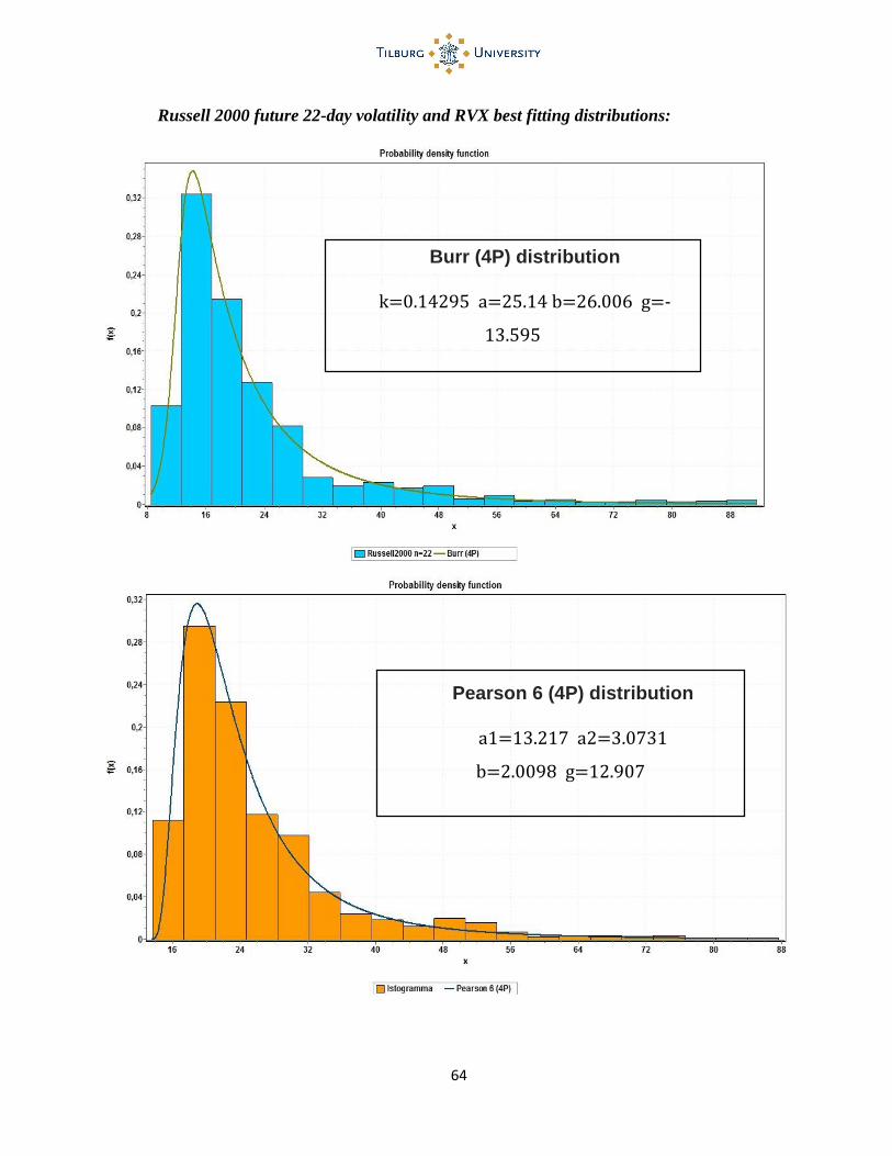
Russell 2000 future 22-day volatility and RVX best fitting distributions:

Burr (4P) distribution

k=0.14295 a=25.14 b=26.006 g=-

13.595

Pearson 6 (4P) distribution

a1=13.217 a2=3.0731

b=2.0098 g=12.907

over the underlying relationship between volatilities of three major u.s. market equity indexes and...

Documents